arX

iv:1

110.

1358

v2 [

cs.D

S] 7

Sep

201

2

Runtime Guarantees for Regression Problems ∗

Hui Han Chin

CMU

hchin@cmu.edu

Aleksander Madry

EPFL

madry@mit.edu

Gary L. Miller

CMU

glmiller@cs.cmu.edu

Richard Peng †‡

CMU

yangp@cs.cmu.edu

September 10, 2012

Abstract

We study theoretical runtime guarantees for a class of optimization problems that occur in a wide va-riety of inference problems. These problems are motivated by the lasso framework and have applicationsin machine learning and computer vision.

Our work shows a close connection between these problems and core questions in algorithmic graphtheory. While this connection demonstrates the difficulties of obtaining runtime guarantees, it alsosuggests an approach of using techniques originally developed for graph algorithms.

We then show that most of these problems can be formulated as a grouped least squares problem,and give efficient algorithms for this formulation. Our algorithms rely on routines for solving quadraticminimization problems, which in turn are equivalent to solving linear systems. Finally we present someexperimental results on applying our approximation algorithm to image processing problems.

∗Partially supported by the National Science Foundation under grant number CCF-1018463.†Supported by a Microsoft Fellowship‡Partially supported by Natural Sciences and Engineering Research Council of Canada (NSERC) under grant number

D-390928-2010.

1 Introduction

The problem of recovering a discrete, clear signal from noisy data is an important problem in signalprocessing. One general approach to this problem is to formulate an objective based on required propertiesof the answer, and then return its minimizer via optimization algorithms. The power of this method was firstdemonstrated in image denoising, where the total variation minimization approach by Rudin, Osher andFatemi [ROF92] had much success. More recent works on sparse recovery led to the theory of compressedsensing [Can06], which includes approaches such as the least absolute shrinkage and selection operator(LASSO) objective due to Tibshirani [Tib96]. These objective functions have proven to be immenselypowerful tools, applicable to problems in signal processing, statistics, and computer vision. In the mostgeneral form, given vector y and a matrix A, one seeks to minimize:

minx||y−Ax||22 (1.1)

subject to: |x|1 ≤ c

It can be shown to be equivalent to the following by introducing a Lagrangian multiplier, λ:

minx||y−Ax||22 + λ|x|1 (1.2)

Many of the algorithms used to minimize the LASSO objective in practice are first order methods[NES07, BCG11], which updates a sequence of solutions using well-defined vectors related to the gradient.These methods are guaranteed to converge well when the matrix A is “well-structured”. The formaldefinition of this well-structuredness is closely related to the conditions required by the guarantees givenin the compressed sensing literature [Can06] for the recovery of a sparse signal. As a result, these methodsperform very well on problems where theoretical guarantees for solution quality are known. This goodperformance, combined with the simplicity of implementation, makes these algorithms the method ofchoice for most problems.

However, LASSO type approaches have also been successfully applied to larger classes of problems. Thishas in turn led to the use of these algorithms on a much wider variety of problem instances. An importantcase is image denoising, where works on LASSO-type objectives predates the compressed sensing literature[ROF92]. The matrices involved here are based on the connectivity of the underlying pixel structure, whichis often a

√n×√n square mesh. Even in a unweighted setting, these matrices tend to be ill-conditioned.

In addition, the emergence of non-local formulations that can connect arbitrary pairs of vertices in thegraph also highlights the need to handle problems that are traditionally considered ill-conditioned. Weshow in Appendix A that the broadest definition of LASSO problems include well-studied problems fromalgorithmic graph theory:

Fact 1.1 Both the s-t shortest path and s-t minimum cut problems in undirected graphs can be solved byminimizing a LASSO objective.

Although linear time algorithms for unweighted shortest path are known, finding efficient parallelalgorithms for this has been a long-standing open problem. The current state of the art parallel algorithmfor finding 1 + ǫ approximate solutions, due to Cohen [Coh00], is quite involved. Furthermore, as thereductions done in Lemma A.1 are readily parallelizable, an efficient algorithm for LASSO minimizationwould also lead to an efficient parallel shortest path algorithm. This suggests that algorithms for minimizingLASSO objectives, where each iteration involve simple, parallelizable operations, are also difficult. Findinga minimum s-t cut with nearly-linear running time is also a long standing open question in algorithm design.

1

In fact, there are known hard instances where many algorithms do exhibit their worst case behavior [JM93].The difficulty of these problems and the non-linear nature of the objective are two of the main challengesin obtaining fast run time guarantees for grouped least squares minimization.

Previous run time guarantees for minimizing LASSO objectives rely on general convex optimizationroutines [BV04], which take at least Ω(n2) time. As the resolution of images are typically at least 256×256,this running time is prohibitive. As a result, when processing image streams or videos in real time, gradientdescent or filtering based approaches are typically used due to time constraints, often at the cost of solutionquality. The continuing increase in problem instance size, due to higher resolution of streaming videos, or3D medical images with billions of voxels, makes the study of faster algorithms an increasingly importantquestion.

While the connection between LASSO and graph problems gives us reasons to believe that the difficultyof graph problems also exists in minimizing LASSO objectives, it also suggests that techniques fromalgorithmic graph theory can be brought to bear. To this end, we draw upon recent developments inalgorithms for maximum flow [CKM+11] and minimum cost flow [DS08]. We show that relatively directmodifications of these algorithms allows us to solve a generalization of most LASSO objectives, which weterm the grouped least squares problem. Our algorithm is similar to convex optimization algorithmsin that each iteration of it solves a quadratic minimization problem, which is equivalent to solving a linearsystem. The speedup over previous algorithms come from the existence of much faster solvers for graphrelated linear systems [ST06], although our approaches are also applicable to situations involving otherunderlying quadratic minimization problems.

The organization of this paper is as follows: In Section 2 we provide a unified optimization problemthat encompasses LASSO, fused LASSO, and grouped LASSO. We then discuss known applications of thegrouped least squares minimization in Section 3 and existing approaches in Section 4. In Section 5 we givetwo algorithms that use solving quadratic minimization problems as underlying routines: An approximatealgorithm based on the maximum flow algorithm of Christiano et al. [CKM+11], and an almost-exactalgorithm that rely on interior point algorithms.

2 Background and Formulations

The formulation of our main problem is motivated by the total variation objective from image denoising.This objective has its origin in the seminal work by Mumford and Shah [MS89]. There are two conflictinggoals in recovering a smooth image from a noisy one, namely that it must be close to the original image,while having very little noise. The Mumford-Shah function models the second constraint by imposingpenalties for neighboring pixels that differ significantly. These terms decrease with the removal of localdistortions, offsetting the higher cost of moving further away from the input. However, the minimizationof this functional is computationally difficult and subsequent works focused on minimizing functions thatare close to it.

The total variation objective is defined for a discrete, pixel representation of the image and measuresnoise using a smoothness term calculated from differences between neighboring pixels. This objective leadsnaturally to a graph G = (V,E) corresponding to the image with pixels. The original (noisy) image isgiven as a vertex labeling s, while the goal of the optimization problem is to recover the ‘true’ image x,which is another set of vertex labels. The requirement of x being close to s is quantified by ||x − s||22,specifically summing over the squares of what we identify as noise while the smoothness term is a sum overabsolute values of difference between adjacent pixels’ labels:

||x− s||22 +∑

(u,v)∈E

|xu − xv| (2.3)

2

This objective can be viewed as an instance of the fused LASSO objective [TSR+05]. As the orientationof the underlying pixel grid is artificially imposed by the camera, this method can introduce rotational biasin its output. One way to correct this bias is to group the differences of each pixel with its 4 neighbors,giving terms of the form:

√

(xu − xv)2 + (xu − xw)2 (2.4)

where v and w are the horizontal and vertical neighbor of u.Our generalization of these objectives is based on the key observation that

√

(xu − xv)2 + (xu − xw)2

and |xu − xv| are both L2 norms of a vector containing differences of values of adjacent pixels. Each suchdifference can be viewed as an edge in the underlying graph, and the grouping gives a natural partition ofthe edges into disjoint sets S1 . . . Sk:

||x− s||22 +∑

1≤i≤k

√

∑

(u,v)∈Si

(xu − xv)2 (2.5)

It can be checked that when each Si contain a single edge, this formulation is identical to the objective inEquation 2.3 since

√

(xu − xv)2 = |xu−xv|. Then all the terms can be written as quadratic positive semi-definite terms involving x and si, where we now allow for different fixed values in the groups. Specificallywhen given symmetric positive semidefinite (PSD) matrices L0 . . .Lk, the objective can be rewritten as:

||x− s0||22 +∑

1≤i≤k

√

(x− si)TLi(x− si) (2.6)

If we use || · ||Lito denote the norm induced by the PSD matrix Li, each of the terms can be written

as ||x− si||Li. To make the first term resemble the other terms in our objective, we will take a square root

of it – as we prove in Appendix D, algorithms that give exact minimizers for this variant still captures theoriginal version of the problem. This simplification allows us to define our main problem:

Definition 2.1 The grouped least squares problem is:Input: n× n matrices L1 . . .Lk and fixed potentials s1 . . . sk ∈ ℜn.Output:

minxOBJ (x) =

∑

1≤i≤k

||x− si||Li

Note that this objective allows for the usual definition of LASSO involving terms of the form |xu| byhaving one group for each such variable with s = 0. It is also related to group LASSO [YL06], whichincorporates similar assumptions about closer dependencies among some of the terms. To our knowledgegrouping has not been studied in conjunction with fused LASSO, although many problems such as theones listed in Section 3 require this generalization.

2.1 Quadratic Minimization and Solving Linear Systems

Our algorithmic approach to the group least squares problem crucially depends on solving a relatedquadratic minimization problem. Specifically, we solve linear systems involving a weighted combination ofthe Li matrices. Let w1 . . .wk ∈ ℜ+ denote weights, where wi is the weight on the ith group. Then thequadratic minimization problem that we consider is:

3

minxOBJ 2(x,w) =

∑

1≤i≤k

1

wi||x− si||2Li

We will use OPT2(w) to denote the minimum value that is attainable. This minimizer, x, can beobtained using the following Lemma:

Lemma 2.2 OBJ 2(x,w) is minimized for x such that

∑

1≤i≤k

1

wiLi

x =∑

1≤i≤k

1

wisi (2.7)

Therefore the quadratic minimization problem reduces to a linear system solve involving∑

i1wi

Li, or∑

i αiLi where α is an arbitrary set of positive coefficients. In general, this can be done in O(nω) time whereω is the matrix multiplication constant [Str69, CW90, VW12]. When Li is symmetric diagonally dominant,which is the case for image applications and most graph problems, these systems can be approximatelysolved to ǫ accuracy in O(m log(1/ǫ)) time, where m is the total number of non-zero entries in the matrices[ST04, ST06, KMP10, KMP11], and also in O(m1/3+θ log(1/ǫ)) parallel depth [BGK+11]. There hasalso been work on extending this type of approach to a wider class of systems [AST09], with works onsystems arising from well-spaced finite-element meshes [BHV04], 2-D trusses [DS07], and certain types ofquadratically coupled flows [KMP12]. For the analysis of our algorithms, we treat this step as a black boxwith running time T (n,m). Furthermore, to simplify our presentation we assume that the solves returnexact answers, as errors can be brought to polynomially small values with an extra O(log n) overhead. Webelieve analyses similar to those performed in [CKM+11, KMP12] can be adapted if we use approximatesolves instead of exact ones.

3 Applications

A variety of problems ranging from computer vision to statistics can be formulated as grouped least squares.We describe some of them below, starting with classical problems from image processing.

3.1 Total Variation Minimization

As mentioned in Section 1, one of the earliest applications of these objectives was in the context of imageprocessing. More commonly known as total variation minimization in this setting [CS05], various variantsof the objective have been proposed with the anisotropic objective the same as Equation 2.3 and theisotropic objective being the one shown in Equation 2.5.

Obtaining a unified algorithm for isotropic and anisotropic TV was one of the main motivations for ourwork. Our result readily applies to both situations, giving approximate algorithms that run in O(m4/3ǫ−8/3)for both cases. It’s worth noting that this guarantee does not rely on the underlying structure of the ofthe graph. This makes the algorithm readily applicable to 3-D images or non-local models involving theaddition of edges across the image . However, when the neighborhoods are those of a 2-D image, a savingby a log n factor can be obtained by using the optimal solver for planar systems by Koutis and Miller[KM07].

3.2 Denoising with Multiple Colors

Most works on image denoising deals with images where each pixel is described using a single numbercorresponding to its intensity. A natural extension would be to colored images, where each pixel has a setof c attributes (in the RGB case, c = 3). One possible analogue of |xi−xj| in this case would be ||xi−xj||2,

4

and this modification can be incorporated by replacing a cluster involving a single edge with clusters overthe c edges between the corresponding pixels.

This type of approach can be viewed as an instance image reconstruction algorithms using Markovrandom fields. Instead of labeling each vertex with a single attribute, a set of c attributes are used insteadand the correlation between vertices is represented using arbitrary PSD matrices. It’s worth remarkingthat when such matrices have bounded condition number, it was shown in [KMP12] that the resulting leastsquares problem can still be solved efficiently by preconditioning with SDD matrices, yielding a similaroverall running time.

3.3 Poisson Image Editing

The Poisson Image Editing method of Perez, Gangnet and Blake [PGB03] is a very popular method forimage blending. This method aims to minimize the difference between the gradient of the image and aguidance field vector v. We show here that the grouped least square problem can be used for minimizingobjectives from this framework. The objective function given in equation (6) of [PGB03]

minf |Ω

∑

(p,q)∩Ω 6=∅

(fp − fq − vpq)2, with fp = f∗

p ,∀p ∈ ∂Ω

comprises mainly of terms of the form:

(xp − xq − vpq)2

This term can be rewritten as ((xp − xq) − (vpq − 0))2. So if we let si be the vector where si,p = vpqand si,q = 0, and Li be the graph Laplacian for the edge connecting p and q, then the term equals to||x − si||2Li

. The other terms on the boundary will have xq as a constant, leading to terms of the form

||xi,p − si,p||22 where si,p = xq. Therefore the discrete Poisson problem of minimizing the sum of thesesquares is an instance of the quadratic minimization problem as described in Section 2.1. Perez et al. inSection 2 of their paper observed that these linear systems are sparse, symmetric and positive definite. Wemake the additional observation here that the systems involved are also symmetric diagonally dominant.The use of the grouped least squares framework also allows the possibility of augmenting these objectiveswith additional L1 or L2 terms.

3.4 Clustering

Hocking et al. [HVBJ11] recently studied an approach for clustering points in d dimensional space. Givena set of points x1 . . . xn ∈ ℜd, one method that they proposed is the minimization of the following objectivefunction:

miny1...yn∈ℜd

n∑

i=1

||xi − yi||22 + λ∑

ij

wij ||yi − yj||2

Where wij are weights indicating the association between items i and j. This problem can be viewedin the grouped least squares framework by viewing each xi and yi as a list of d variables, giving thatthe ||xi − yi||2 and ||yi − yj||2 terms can be represented using a cluster of d edges. Hocking et al. usedthe Frank-Wolfe algorithm to minimize a relaxed form of this objective and observed fast behavior inpractice. In the grouped least squares framework, this problem is an instance with O(n2) groups andO(dn2) edges. Combining with the observation that the underlying quadratic optimization problems canbe solved efficiently allows us to obtain an 1 + ǫ approximate solution in O(dn8/3ǫ−8/3) time.

5

4 Previous Algorithmic Results

Due to the importance of optimization problems motivated by LASSO there has been much work on efficientalgorithms for them. We briefly describe some of the previous approaches for LASSO minimization below.

4.1 Second-order Cone Programming

To the best of our knowledge, the only algorithms that provide robust worst-case bounds for the entire classof grouped least squares problems are based on applying tools from convex optimization. In particular, itis known that interior point methods applied to these problems converge in O(

√k) iterations with each

iterations requiring solving a certain linear system [BV04, GY04]. Unfortunately, computing these solutionsis computationally expensive – the best previous bound for solving one of these systems is O(mω) whereω is the matrix multiplication exponent. This results in fairly large O(m1/2+ω) total running time andcontributes to the popularity of first-order methods described above in practical scenarios. We will revisitthis approach in Subsection 5.2 and show an improved algorithm for the inner iterations. However, itsrunning time still has a fairly large dependency on k.

4.2 Graph Cuts

For the anisotropic total variation objective shown in Equation 2.3, a minimizer can be found by solving alarge number of almost-exact maximum flow calls [DS06, KZ04]. Although the number of iterations can belarge, these works show that the number of problem instances that a pixel can appear in is small. Combiningthis reduction with the fastest known exact algorithm for the maximum flow problem by Goldberg andRao [GR98] gives an algorithm that runs in O(m3/2) time.

It’s worth mentioning that both of these algorithms requires extracting the minimum cut in order toconstruct the problems for subsequent iterations. As a result, it’s not clear whether recent advances onfast approximations of maximum flow and minimum s-t cuts [CKM+11] can be used as a black box withthese algorithms. Extending this approach to the non-linear isotropic objective also appears to be difficult.

4.3 Iterative Reweighted Least Squares

An approach similar to convex optimization methods, but has much better observed rates of convergenceis the iterative reweighted least squares (IRLS) method. This method does a much more aggressive ad-justment each iteration and to give good performances in practice [WR07].

4.4 First Order Methods

The method of choice in practice are first order methods such as [NES07, BCG11]. Theoretically thesemethods are known to converge rapidly when the objective function satisfies certain Lipschitz conditions.Many of the more recent works on first order methods focus on lowering the dependency of ǫ under theseconditions. As discussed in Section 1 and Appendix A, this direction can be considered orthogonal to ourguarantees as the grouped least squares problem is a significantly more general formulation.

5 Solving Grouped Least Squares Using Quadratic Minimizations

In this section, we show two algorithms for the grouped least squares problem based on direct adaptationsof state-of-the-art algorithms for maximum flow [CKM+11] and minimum cost flow [DS08]. Our guaranteescan be viewed as reductions to the quadratic minimization problems described in Section 2.1. As a result,they imply efficient algorithms for problems where fast algorithms are known for the corresponding leastsquares problems. The analyses of these algorithms are intricate, but mostly follow the presentations in[CKM+11, DS08, BV04]. They’re presented in Appendices B and C.

5.1 Approximate Algorithm

Our first algorithm is based on the electrical flow based maximum flow and minimum cut algorithm byChristiano et al. [CKM+11]. Recall that the minimum s-t cut problem - equivalent to an L1-minimization

6

problem - is a special case of the grouped least squares problem where each edge belongs to its owngroup(i.e., k = m). As a result, it’s natural to extend the approach of [CKM+11] to the whole spectrumof values of k by treating each group as an ’edge’.

One view of the cut algorithm from [CKM+11] is that it places a weight on each group, and minimizesa quadratic, or L2

2 problem involving terms of the from 1wi||x− si||2Li

. These weights are adjusted using themultiplicative weights update framework [AHK05, LW94] based on the energy of each group. The terms||x− si||Li

and 1wi||x− si||2Li

are equal when wi = ||x− si||Li. Therefore, one natural view of this routine is

that it gradually adjusts the weights to become a scaled copy of ||x− si||Li. This leads to a simplification

of the Christiano et al. algorithm, whose update requires a flow obtained from the dual of the quadraticminimization problem. Pseudocode of the algorithm is shown in Algorithm 1.

Algorithm 1 Algorithm for the approximate decision problem of whether there exist vertex potentialswith objective at most OPT

ApproxGroupedLeastSquares

Input: PSD matrices L1 . . .Lk, fixed values s1 . . . sk for each group. Routine Solve for solving linearsystems, width parameter ρ and error bound ǫ.Output: Vector x such that OBJ (x) ≤ (1 + 10ǫ)OPT.

1: Initialize w(0)i = 1 for all 1 ≤ i ≤ k

2: N ← 10ρ log nǫ−2

3: for t = 1 . . . N do

4: µ(t−1) ←∑

i w(t−1)i

5: Use Solve to compute a minimizer for the quadratic minimization problem where αi =1

w(t−1)i

, let

this solution be x(t)

6: Let λ(t) =√

µ(t−1)OBJ 2(x(t))

7: Update the weight of each group: w(t)i ← w

(t−1)i +

(

ǫρ

||x(t)−si||Li

λ(t) + 2ǫ2

kρ

)

µ(t−1)

8: end for

9: t← argmin0≤t≤N OBJ (x(t))10: return x(t)

The main difficulty of analyzing this algorithm is that the analysis of minimum s-t cut algorithm of[CKM+11] relies strongly on the existence of a solution where x is either 0 or 1. Our analysis extends thispotential function into the fractional setting via. a function based on the Kulback-Liebler (KL) divergence[KL51]. To our knowledge the use of this potential with multiplicative weights was first introduced byFreund and Schapire [FS99], and is common in learning theory. This function can be viewed as measuring

the KL-divergence between w(t)i and ||x − si||Li

over all groups, where x an optimum solution to thegrouped least squares problem. Formally, the KL divergence between these two vectors is:

DKL =∑

i

||x− si||Lilog

(

||x− si||Li

w(t)i

)

(5.8)

Subtracting the constant term given by∑

i ||x− si||L(t)i

log(||x − si||L(t)i

) and multiplying by −1/OPT

gives us our key potential function, ν(t):

7

ν(t) =1

OPT

∑

i

||x− si||Lilog(w

(t)i ) (5.9)

It’s worth noting that in the case of the cut algorithm, this function is identical to the potential functionused in [CKM+11]. We show the convergence of our algorithm by proving that if the solution produced insome iteration is far from optimal, ν(t) increases substantially. Upper bounding it with a term related tothe sum of weights, µ(t) allows us to prove convergence. The full proof is given in Appendix B.

To simplify the analysis, we assume that the guess that we’re trying to solve the decision problemon, OPT, all entries of s, and spectrum of Li are polynomially bounded in n. That is, there exist someconstant d such that −nd ≤ si,u ≤ nd and n−dI ∑i Li ndI where A B means B−A is PSD. Someof these assumptions can be relaxed via. analyses similar to Section 2 of [CKM+11].

Theorem 5.1 On input of an instance of OBJ with edges partitioned into k sets. If all parameterspolynomially bounded between n−d and nd, running ApproxGroupedLeastSquares with ρ = 2k1/3ǫ−2/3

returns a solution x with such that OBJ (x) ≤ max(1 + 10ǫ)OPT, n−d where OPT is the value of theoptimum solution.

The additive n−d case is included to deal with the case where OPT = 0, or is close to it. We believe itshould be also possible to handle this case via. condition numbers restrictions on

∑

i Li.

5.2 Almost-Exact Algorithm

We now show improved algorithms for solving the second order cone programming formulation given in[BV04, GY04]. It was shown in [DS08] that in the linear case, as with graph problems such as maximumflow, minimum cost flow and shortest path, interior point algorithms reduce the problem to solving O(m1/2)symmetrically diagonally dominant linear systems. The grouped least squares formulation creates artifactsthat perturb the linear systems generated by the interior point algorithms, making the resulting systemboth more difficult to interpret and to solve. However, the iteration count of this approach also onlydepends on k, [GY04, BV04], and has a better dependency on ǫ of O(log(1/ǫ)).

There are various ways to solve the grouped least squares problem using interior point algorithms. Wefollow the log-barrier method, as presented in Boyd and Vandenberghe [BV04] here for simplicity. Thisformulation defines one extra variable yi for each group and enforces yi ≥ ||x − si||Li

using the barrierfunction φi(x, yi) = log(y2i − ||x − si||2Li

). Minimizing t · (∑i yi) for gradually increasing values of t givesthe following sequence of functions to minimize:

f(t,x,y) = t∑

i

yi −∑

i

log(y2i − ||x− si||2Li) (5.10)

Various interior point algorithms have been proposed, one commonality that they have is finding anupdate direction by solving a linear system. The iteration guarantees for recovering almost exact solutioncan be characterized as follows:

Lemma 5.2 (Section 11.5.3 from [BV04]) A solution that’s within additive ǫ of the optimum solution canbe produced in O(k1/2 log(1/ǫ)) steps, each of which requires solving a linear system involving ∇2f(t,x,y)for some value of t, x and y.

These systems are examined in detail in Appendix C. Since the t∑

i yi term is linear, it can be omittedfrom the Hessian, leaving

∑

i∇2φ(x, yi). We then check that the barrier term yi creates a low rank

8

perturbation to the Li term, which is the Hessian for ||x − si||2Li. By taking Schur complements and

applying the Sherman-Morrison-Woodbury identity on inverses for low rank perturbations, we arrive atthe following observation in Appendix C:

Theorem 5.3 Suppose there is an algorithm for solving linear systems of the form∑

i αiLi in T (n,m)time where m. For any choice of x,y, a linear system involving the Hessian of φ(x,y), ∇2φ(x,y) can besolved in O(kω + kT (n,m) + k2n) time.

Combining this with the iteration count of O(k1/2 log(1/ǫ)) gives a total running time of O((kω+1/2 +k3/2T (n,m) + k5/2n) log(1/ǫ)).

6 Experimental Results

We performed a series of experiments using the approximate algorithm described in Section 5.1. TheSDD linear systems that arise in the quadratic minimization problems were solved using the combinatorialmultigrid (CMG) solver [KM09, KMT09]. One side observation from our experiments is that for the sparseSDD linear systems that arise from image processing, the CMG solver yields good results both in accuracyand running time.

6.1 Total Variational Denoising

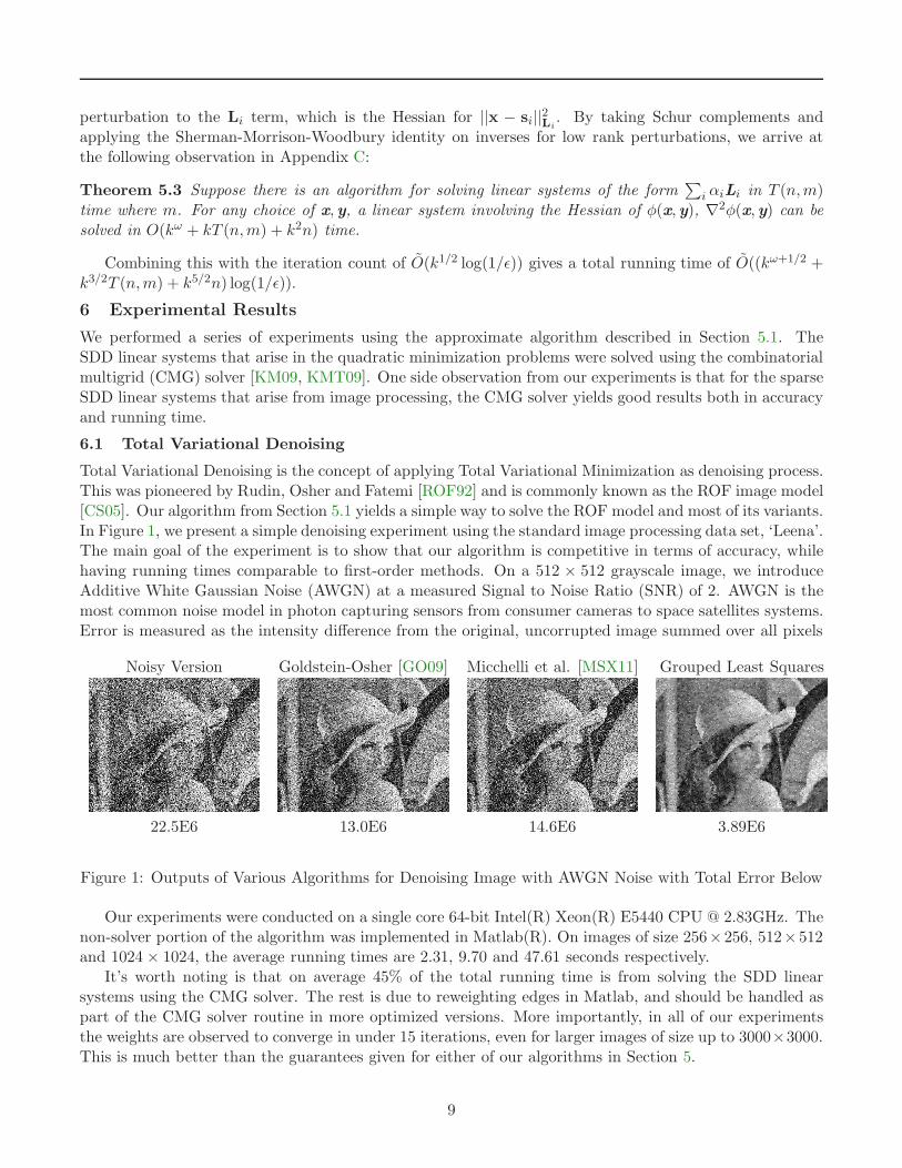
Total Variational Denoising is the concept of applying Total Variational Minimization as denoising process.This was pioneered by Rudin, Osher and Fatemi [ROF92] and is commonly known as the ROF image model[CS05]. Our algorithm from Section 5.1 yields a simple way to solve the ROF model and most of its variants.In Figure 1, we present a simple denoising experiment using the standard image processing data set, ‘Leena’.The main goal of the experiment is to show that our algorithm is competitive in terms of accuracy, whilehaving running times comparable to first-order methods. On a 512 × 512 grayscale image, we introduceAdditive White Gaussian Noise (AWGN) at a measured Signal to Noise Ratio (SNR) of 2. AWGN is themost common noise model in photon capturing sensors from consumer cameras to space satellites systems.Error is measured as the intensity difference from the original, uncorrupted image summed over all pixels

Noisy Version Goldstein-Osher [GO09] Micchelli et al. [MSX11] Grouped Least Squares

22.5E6 13.0E6 14.6E6 3.89E6

Figure 1: Outputs of Various Algorithms for Denoising Image with AWGN Noise with Total Error Below

Our experiments were conducted on a single core 64-bit Intel(R) Xeon(R) E5440 CPU @ 2.83GHz. Thenon-solver portion of the algorithm was implemented in Matlab(R). On images of size 256×256, 512×512and 1024 × 1024, the average running times are 2.31, 9.70 and 47.61 seconds respectively.

It’s worth noting is that on average 45% of the total running time is from solving the SDD linearsystems using the CMG solver. The rest is due to reweighting edges in Matlab, and should be handled aspart of the CMG solver routine in more optimized versions. More importantly, in all of our experimentsthe weights are observed to converge in under 15 iterations, even for larger images of size up to 3000×3000.This is much better than the guarantees given for either of our algorithms in Section 5.

9

6.2 Image Processing

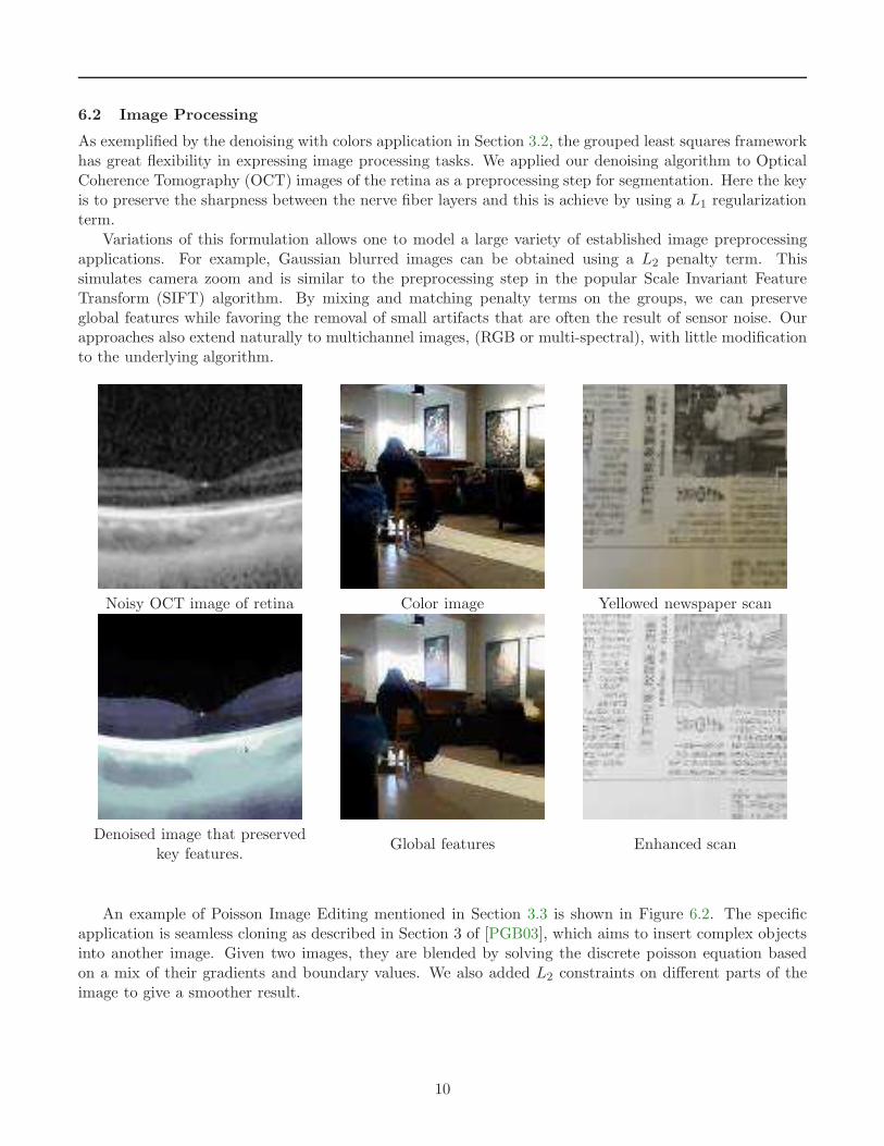
As exemplified by the denoising with colors application in Section 3.2, the grouped least squares frameworkhas great flexibility in expressing image processing tasks. We applied our denoising algorithm to OpticalCoherence Tomography (OCT) images of the retina as a preprocessing step for segmentation. Here the keyis to preserve the sharpness between the nerve fiber layers and this is achieve by using a L1 regularizationterm.

Variations of this formulation allows one to model a large variety of established image preprocessingapplications. For example, Gaussian blurred images can be obtained using a L2 penalty term. Thissimulates camera zoom and is similar to the preprocessing step in the popular Scale Invariant FeatureTransform (SIFT) algorithm. By mixing and matching penalty terms on the groups, we can preserveglobal features while favoring the removal of small artifacts that are often the result of sensor noise. Ourapproaches also extend naturally to multichannel images, (RGB or multi-spectral), with little modificationto the underlying algorithm.

Noisy OCT image of retina Color image Yellowed newspaper scan

Denoised image that preservedkey features.

Global features Enhanced scan

An example of Poisson Image Editing mentioned in Section 3.3 is shown in Figure 6.2. The specificapplication is seamless cloning as described in Section 3 of [PGB03], which aims to insert complex objectsinto another image. Given two images, they are blended by solving the discrete poisson equation basedon a mix of their gradients and boundary values. We also added L2 constraints on different parts of theimage to give a smoother result.

10

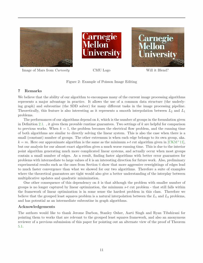
Image of Mars from Curiosity CMU Logo Will it Blend?

Figure 2: Example of Poisson Image Editing

7 Remarks

We believe that the ability of our algorithm to encompass many of the current image processing algorithmsrepresents a major advantage in practice. It allows the use of a common data structure (the underly-ing graph) and subroutine (the SDD solver) for many different tasks in the image processing pipeline.Theoretically, this feature is also interesting as it represents a smooth interpolation between L2 and L1

problems.The performances of our algorithms depend on k, which is the number of groups in the formulation given

in Definition 2.1. , it gives them provable runtime guarantees. Two settings of k are helpful for comparisonto previous works. When k = 1, the problem becomes the electrical flow problem, and the running timeof both algorithms are similar to directly solving the linear system. This is also the case when there is asmall (constant) number of groups. The other extremum is when each edge belongs to its own group, aka.k = m. Here our approximate algorithm is the same as the minimum s-t cut algorithm given in [CKM+11],but our analysis for our almost exact algorithm gives a much worse running time. This is due to the interiorpoint algorithm generating much more complicated linear systems, and actually occur when most groupscontain a small number of edges. As a result, finding faster algorithms with better error guarantees forproblems with intermediate to large values of k is an interesting direction for future work. Also, preliminaryexperimental results such as the ones from Section 6 show that more aggressive reweightings of edges leadto much faster convergence than what we showed for our two algorithms. Therefore a suite of exampleswhere the theoretical guarantees are tight would also give a better understanding of the interplay betweenmultiplicative updates and quadratic minimization.

One other consequence of this dependency on k is that although the problem with smaller number ofgroups is no longer captured by linear optimization, the minimum s-t cut problem - that still falls withinthe framework of linear optimization is in some sense the hardest problem in this class. Therefore webelieve that the grouped least squares problem is a natural interpolation between the L1 and L2 problems,and has potential as an intermediate subroutine in graph algorithms.

Acknowledgements

The authors would like to thank Jerome Darbon, Stanley Osher, Aarti Singh and Ryan Tibshirani forpointing them to works that are relevant to the grouped least squares framework, and also an anonymousreviewer of a previous submission of this paper for pointing out an alternate view of the proof of Theorem5.1.

11

References

[AHK05] Sanjeev Arora, Elad Hazan, and Satyen Kale. The multiplicative weights update method: a metaalgorithm and applications. Technical report, Princeton University, 2005. 5.1

[AST09] Haim Avron, Gil Shklarski, and Sivan Toledo. On element SDD approximability. CoRR, abs/0911.0547,2009. 2.1

[BCG11] Stephen R. Becker, Emmanuel J. Candes, and Michael Grant. Templates for convex cone problems withapplications to sparse signal recovery. MATHEMATICAL PROGRAMMING COMPUTATION, 3:165,2011. 1, 4.4

[BGK+11] Guy E. Blelloch, Anupam Gupta, Ioannis Koutis, Gary L. Miller, Richard Peng, and Kanat Tangwongsan.Near linear-work parallel SDD solvers, low-diameter decomposition, and low-stretch subgraphs. In Pro-ceedings of the 23rd ACM symposium on Parallelism in algorithms and architectures, SPAA ’11, pages13–22, New York, NY, USA, 2011. ACM. 2.1

[BHV04] Erik G. Boman, Bruce Hendrickson, and Stephen A. Vavasis. Solving elliptic finite element systems innear-linear time with support preconditioners. CoRR, cs.NA/0407022, 2004. 2.1

[BV04] S. Boyd and L. Vandenberghe. Convex Optimization. Camebridge University Press, 2004. 1, 4.1, 5, 5.2,5.2

[Can06] J. Candes, E. Compressive sampling. Proceedings of the International Congress of Mathematicians, 2006.1, 1

[CKM+11] Paul Christiano, Jonathan A. Kelner, Aleksander Madry, Daniel Spielman, and Shang-Hua Teng. Elec-trical Flows, Laplacian Systems, and Faster Approximation of Maximum Flow in Undirected Graphs. InProceedings of the 43rd ACM Symposium on Theory of Computing (STOC), 2011. 1, 2.1, 4.2, 5, 5.1, 5.1,5.1, 7, B

[Coh00] Edith Cohen. Polylog-time and near-linear work approximation scheme for undirected shortest paths. J.ACM, 47(1):132–166, 2000. 1

[CS05] Tony Chan and Jianhong Shen. Image Processing And Analysis: Variational, Pde, Wavelet, And Stochas-tic Methods. SIAM, 2005. 3.1, 6.1

[CW90] D. Coppersmith and S. Winograd. Matrix multiplication via arithmetical progressions. J. SymbolicComputation, 9:251–280, 1990. 2.1

[DS06] Jerome Darbon and Marc Sigelle. Image restoration with discrete constrained total variation part i: Fastand exact optimization. Journal of Mathematical Imaging and Vision, 26(3):261–276, 2006. 4.2

[DS07] Samuel I. Daitch and Daniel A. Spielman. Support-graph preconditioners for 2-dimensional trusses.CoRR, abs/cs/0703119, 2007. 2.1

[DS08] Samuel I. Daitch and Daniel A. Spielman. Faster approximate lossy generalized flow via interior pointalgorithms. In Proceedings of the 40th annual ACM symposium on Theory of computing, STOC ’08,pages 451–460, New York, NY, USA, 2008. ACM. 1, 5, 5.2, A

[FS99] Yoav Freund and Robert E. Schapire. Adaptive game playing using multiplicative weights. Games andEconomic Behavior, 29(1-2):79–103, October 1999. 5.1

[GO09] Tom Goldstein and Stanley Osher. The split Bregman method for l1-regularized problems. SIAM J.Img. Sci., 2:323–343, April 2009. 6.1

[GR98] Andrew V. Goldberg and Satish Rao. Beyond the flow decomposition barrier. J. ACM, 45:783–797,September 1998. 4.2

[GY04] Donald Goldfarb and Wotao Yin. Second-order cone programming methods for total variation-basedimage restoration. SIAM J. Sci. Comput, 27:622–645, 2004. 4.1, 5.2

[HVBJ11] Toby Hocking, Jean-Philippe Vert, Francis Bach, and Armand Joulin. Clusterpath: an algorithm forclustering using convex fusion penalties. In Lise Getoor and Tobias Scheffer, editors, Proceedings of the28th International Conference on Machine Learning (ICML-11), ICML ’11, pages 745–752, New York,NY, USA, June 2011. ACM. 3.4

[JM93] David S. Johnson and Catherine C. McGeoch, editors. Network Flows and Matching: First DIMACSImplementation Challenge. American Mathematical Society, Boston, MA, USA, 1993. 1

[KL51] S. Kullback and R. A. Leibler. On information and sufficiency. Ann. Math. Statist., 22(1):79–86, 1951.5.1

12

[KM07] Ioannis Koutis and Gary L. Miller. A linear work, O(n1/6) time, parallel algorithm for solving planarLaplacians. In Proc. 18th ACM-SIAM Symposium on Discrete Algorithms (SODA 2007), 2007. 3.1

[KM09] Ioannis Koutis and Gary Miller. The combinatorial multigrid solver. Conference Talk, March 2009. 6

[KMP10] Ioannis Koutis, Gary L. Miller, and Richard Peng. Approaching optimality for solving SDD systems.CoRR, abs/1003.2958, 2010. 2.1

[KMP11] Ioannis Koutis, Gary L. Miller, and Richard Peng. Solving sdd linear systems in time O(m logn log(1/ǫ)).CoRR, abs/1102.4842, 2011. 2.1

[KMP12] Jonathan A. Kelner, Gary L. Miller, and Richard Peng. Faster approximate multicommodity flow usingquadratically coupled flows. In Proceedings of the 44th symposium on Theory of Computing, STOC ’12,pages 1–18, New York, NY, USA, 2012. ACM. 2.1, 3.2

[KMT09] Ioannis Koutis, Gary L. Miller, and David Tolliver. Combinatorial preconditioners and multilevel solversfor problems in computer vision and image processing. In International Symposium of Visual Computing,pages 1067–1078, 2009. 6

[KZ04] Vladimir Kolmogorov and Ramin Zabih. What energy functions can be minimized via graph cuts. IEEETransactions on Pattern Analysis and Machine Intelligence, 26:65–81, 2004. 4.2

[LW94] Nick Littlestone and Manfred K. Warmuth. The weighted majority algorithm. Inf. Comput., 108(2):212–261, February 1994. 5.1

[MS89] D. Mumford and J. Shah. Optimal approximations by piecewise smooth functions and associated varia-tional problems. Communications on Pure and Applied Mathematics, 42:577–685, 1989. 2

[MSX11] Charles A Micchelli, Lixin Shen, and Yuesheng Xu. Proximity algorithms for image models: denoising.Inverse Problems, 27(4):045009, 2011. 6.1

[MVV87] K. Mulmuley, U. V. Vazirani, and V. V. Vazirani. Matching is as easy as matrix inversion. Combinatorica,7(1):105–113, January 1987. A

[NES07] Yu. NESTEROV. Gradient methods for minimizing composite objective function. CORE DiscussionPapers 2007076, Universit catholique de Louvain, Center for Operations Research and Econometrics(CORE), 2007. 1, 4.4

[PGB03] P. Prez, M. Gangnet, and A. Blake. Poisson image editing. ACM Transactions on Graphics (SIG-GRAPH’03), 22(3):313–318, 2003. 3.3, 6.2

[ROF92] L. Rudin, S. Osher, and E. Fatemi. Nonlinear total variation based noise removal algorithm. Physica D,1(60):259–268, 1992. 1, 1, 6.1

[ST04] Daniel A. Spielman and Shang-Hua Teng. Nearly-linear time algorithms for graph partitioning, graphsparsification, and solving linear systems. In Proceedings of the 36th Annual ACM Symposium on Theoryof Computing, pages 81–90, June 2004. 2.1

[ST06] Daniel A. Spielman and Shang-Hua Teng. Nearly-linear time algorithms for preconditioning and solvingsymmetric, diagonally dominant linear systems. CoRR, abs/cs/0607105, 2006. 1, 2.1

[Str69] Volker Strassen. Gaussian elimination is not optimal. Numerische Mathematik, 13:354–356, 1969. 2.1

[Tib96] R. Tibshirani. Regression shrinkage and selection via the lasso. Journal of the Royal Statistical Society(Series B), 58:267–288, 1996. 1

[TSR+05] Robert Tibshirani, Michael Saunders, Saharon Rosset, Ji Zhu, and Keith Knight. Sparsity and smooth-ness via the fused lasso. Journal of the Royal Statistical Society Series B, 67(1):91–108, 2005. 2

[VW12] Virginia Vassilevska Williams. Breaking the Coppersmith-Winograd barrier. In Proceedings of the 44thsymposium on Theory of Computing, STOC ’12, 2012. 2.1

[WR07] B. Wohlberg and P. Rodriguez. An iteratively reweighted norm algorithm for minimization of totalvariation functionals. Signal Processing Letters, IEEE, 14(12):948 –951, dec. 2007. 4.3

[YL06] Ming Yuan and Yi Lin. Model selection and estimation in regression with grouped variables. Journal ofthe Royal Statistical Society, Series B, 68:49–67, 2006. 2

13

A Proofs about Graph Problems as Minimizing LASSO Objectives

In this section we give formal proofs that show the shortest path problem is an instance of LASSO andthe minimum cut problem is an instance of fused-LASSO.

It’s worth noting that our proofs do not guarantee that the answers returned are a single path or cut.In fact, when multiple solutions have the same value it’s possible for our algorithm to return a linearcombination of them. However, we can ensure that the optimum solution is unique using the IsolationLemma of Mulmuley, Vazarani and Vazarani [MVV87] while only incurring polynomial increase in edgelengths/weights. This analysis is similar to the one in Section 3.5 of [DS08] for finding a unique minimumcost flow, and is omitted here.

We prove the two claims in Fact 1.1 about shortest path and minimum cut separately in Lemmas A.1and A.2.

Lemma A.1 Given a s-t shortest path instance in an undirected graph where edge lengths l : E → ℜ+

are integers between 1 and nd. There is a LASSO minimization instance where all entries are bounded bynO(d) such that the value of the LASSO minimizer is within 1 of the optimum answer.

Proof Our reductions rely crucially on the edge-vertex incidence matrix, which we denote using B.Entries of this matrix are defined as follows:

Be,u =

−1 if u is the head of e1 if u is the tail of e0 otherwise

(1.11)

We first show the reduction for shortest path. Then a path from s to t corresponds to a flow valueassigned to all edges, f : E → ℜ such that BT f = χs,t. If we have another flow f′ corresponding to anypath from s to t, then this constraint can be written as:

||BT f− χs,t||2 =0 (1.12)

||BT (f− f′)||2 =0

||f− f′||BB

T =0 (1.13)

(1.14)

The first constraint is closer to the classical LASSO problem while the last one is within our definitionof grouped least squares problem. The length of the path can then be written as

∑

e le|fe|. Weightingthese two terms together gives:

minf

λ||f− f′||2BB

T +∑

e

le|fe| (1.15)

Where the maximum entry is bounded by maxnd, n2λ. Clearly its objective is less than the length ofthe shortest path, let this solution be f. Then since the total objective is at most nd+1, we have that themaximum deviation between BT f and χs,t is at most nd+1/λ. Then given a spanning tree, each of thesedeviations can be routed to s or t at a cost of at most nd+1 per unit of flow. Therefore we can obtain f′ suchthat BT f′ = χs,t whose objective is bigger by at most n2d+2/λ. Therefore setting λ = n2d+2 guaranteesthat our objective is within 1 of the length of the shortest path, while the maximum entry in the problemis bounded by nO(d).

14

We now turn our attention to the minimum cut problem, which can be formulated as finding a vertex

labeling x(vert) where x(vert)s = 0, x

(vert)t = 1 and the size of the cut,

∑

uv∈E |x(vert)u − x

(vert)v |. Since the

L1 term in the objective can incorporate single variables, we use an additional vector x(edge) to indicatedifferences along edges. The minimum cut problem then becomes minimizing |x(edge)| subject to theconstraint that x(edge) = B′x(vert)′ +Bχt, where B

′ and x(vert)′ are restricted to vertices other than s and tand χt is the indicator vector that’s 1 on t. The equality constraints can be handled similar to the shortestpath problem by increasing the weights on the first term. One other issue is that |x(vert)′ | also appears inthe objective term, and we handle this by scaling down x(vert)′ , or equivalently scaling up B′.

Lemma A.2 Given a s-t minimum cut instance in an undirected graph where edge weights w : E → ℜ+

are integers between 1 and nd. There is a LASSO minimization instance where all entries are bounded bynO(d) such that the value of the LASSO minimizer is within 1 of the minimum cut.

Proof

Consider the following objective, where λ1 and λ2 are set to nd+3 and n2:

λ1||λ2B′x(vert)′ +Bχt − x(edge)||22 + |x(vert′)|1 + |x(edge)|1 (1.16)

Let x be an optimum vertex labelling, then setting x(vert′) to the restriction of n−2x on vertices otherthan s and t and x(edge) to Bx(vert) makes the first term 0. Since each entry of x is between 0 and 1, theadditive increase caused by |x(vert′)|1 is at most 1/n. Therefore this objective’s optimum is at most 1/nmore than the size of the minimum cut.

For the other direction, consider any solution x(vert)′ ,x(edge)′ whose objective is at most 1/n more thanthe size of the minimum cut. Since the edge weights are at most nd and s has degree at most n, the totalobjective is at most nd+1 + 1. This gives:

||λ2B′x(vert)′ +Bχt − x(edge)||22 ≤n−1 (1.17)

||λ2B′x(vert)′ +Bχt − x(edge)||1 ≤||λ2B

′x(vert)′ +Bχt − x(edge)||2 ≤ n−1/2 (1.18)

Therefore changing x(edge) to λ2B′x(vert)′ + Bχt increases the objective by at most n−1/2 < 1. This

gives a cut with weight within 1 of the objective value and completes the proof.

We can also show a more direct connection between the minimum cut problem and the fused LASSOobjective, where each absolute value term may contain a linear combination of variables. This formulationis closer to the total variation objective, and is also an instance of the problem formulated in Definition2.1 with each edge in a group.

Lemma A.3 The minimum cut problem in undirected graphs can be written as an instance of the fusedLASSO objective.

Proof Given a graph G = (V,E) and edge weights cost, the problem can be formulated as labeling thevertices of V \ s, t in order to minimize:

∑

uv∈E,u,v∈V \s,t

costuv|xu − xv|+∑

su∈E,u∈V \s,t

costsu|xu − 0|+∑

ut∈E,u∈V \s,t

costut|xu − 1| (1.19)

15

B Multiplicative Weights Based Approximate Algorithm

In this section we show that the approximate algorithm described in Section 5.1 finds a solution close to theoptimum. We first show that if λ(t) as defined on Line 6 of Algorithm 1 is an upper bound for OBJ (x(t).This is crucial in our use of it as the normalizing factor in our update step on Line 7.

Lemma B.1 In all iterations we have:

OBJ (x(t)) ≤ λ(t)

Proof By the Cauchy-Schwarz inequality we have:

(λ(t))2 =

(

∑

i

w(t−1)i

)(

∑

i

1

w(t−1)i

||x(t) − si||2Li

)

≥(

∑

i

||x(t) − si||Li

)2

=OBJ (x(t))2 (2.20)

Taking square roots of both sides completes the proof.

At a high level, the algorithm assigns weights wi for each group, and iteratively reweighs them for Niterations. Recall that our key potential functions are µ(t) which is the sum of weights of all groups, and:

ν(t) =1

OPT

∑

i

||x− si||Lilog(w

(t)i ) (2.21)

Where x is a solution such that OBJ (x) = OPT. We will show that if OBJ (x(t)), or in turn λ(t) islarge, then ν(t) increases at a rate substantially faster than µ(t). These bounds, and the relation betweenµ(t) and ν(t) is summarized below:

Lemma B.2 1.

ν(t) ≤ log(µ(t)) (2.22)

2.

µ(t) ≤(

1 +ǫ(1 + 2ǫ)

ρt

)

µ(t−1) (2.23)

and

log(µ(t)) ≤ ǫ(1 + 2ǫ)

ρt+ log k (2.24)

3. If in iteration t, λ(t) ≥ (1 + 10ǫ)OPT and ||x− si||Li≤ ρ

w(t−1)i

µ(t−1) λ(t) for all groups i, then:

16

νt ≥ ν(t−1) +ǫ(1 + 9ǫ)

ρ(2.25)

The relationship between the upper and lower potentials can be established using the fact that wi isnon-negative:

Proof of Lemma B.2, Part 1:

ν(t) =1

OPT

∑

i

||x− si||Lilog(w

(t)i )

≤ 1

OPT

∑

i

||x− si||Lilog

∑

j

w(t)j

= log(µ(t))

(

1

OPT

∑

i

||x− si||Li

)

≤ log(µ(t)) (2.26)

Part 2 follows directly from the local behavior of the log function:

Proof of Lemma B.2, Part 2: The update rules gives:

µ(t) =∑

i

w(t)i

=∑

i

w(t−1)i +

(

ǫ

ρ

||x(t) − si||Li

λ(t)+

2ǫ2

kρ

)

µ(t−1)

by update rule on Line 7 of GroupedLeastSquares

=µ(t−1) +ǫ

ρ

∑

i ||x(t) − si||Li

λ(t)µ(t−1) +

∑

i

2ǫ2

kρµ(t−1)

=µ(t−1) +ǫ

ρ

OBJ (x(t))

λ(t)µ(t−1) +

2ǫ2

ρµ(t−1)

≤µ(t−1) +ǫ

ρµ(t−1) +

2ǫ2

ρµ(t−1) By Lemma B.1

=

(

1 +ǫ(1 + 2ǫ)

ρ

)

µ(t−1) (2.27)

Using the fact that 1 + x ≤ exp(x) when x ≥ 0 we get:

17

µ(t) ≤ exp

(

ǫ(1 + 2ǫ)

ρ

)

µ(t−1)

≤ exp

(

tǫ(1 + 2ǫ)

ρ

)

µ(0)

=exp

(

tǫ(1 + 2ǫ)

ρ

)

k

Taking logs of both sides gives Equation 2.24.

This upper bound on the value of µt also allows us to show that the balancing rule keeps the wtis

reasonably balanced within a factor of k of each other. The following corollary can also be obtained.

Corollary B.3 The weights at iteration t satisfy w(t)i ≥ ǫ

kµ(t).

Proof

The proof is by induction on t. When t = 0 we have w(0)i = 1, µ(0) = k and the claim follows from

ǫkk = ǫ < 1. When t > 1, we have:

w(t)i ≥w

(t−1)i +

2ǫ2

kρµ(t−1) By line 7

≥(

ǫ

k+

2ǫ2

kρ

)

µ(t−1) By the inductive hypothesis

=ǫ

k

(

1 +2ǫ

ρ

)

µ(t−1)

≥ ǫ

k

(

1 +ǫ(1 + 2ǫ)

ρ

)

µ(t−1)

≥ ǫ

kµ(t) By Lemma B.2, Part 2 (2.28)

The proof of Part 3 is the key part of our analysis. The first order change of ν(t) is written as a sum ofproducts of L2 norms, which we analyze via. the fact that x(t) is the solution of a linear system from thequadratic minimization problem.

Proof of Lemma B.2, Part 3:

We make use of the following known fact about the behavior of the log function around 1:

Fact B.4 If 0 ≤ x ≤ ǫ, then log(1 + x) ≥ (1− ǫ)x.

18

ν(t) − ν(t−1) =1

OPT

∑

1≤i≤k

||x− si||Lilog(

w(t)i

)

− 1

OPT

∑

1≤i≤k

||x− si||Lilog(

w(t−1)i

)

By Equation 2.21

=1

OPT

∑

1≤i≤k

||x− si||Lilog

(

w(t)i

w(t−1)i

)

≥ 1

OPT

∑

1≤i≤k

||x− si||Lilog

(

1 +ǫ

ρ

||x(t) − si||Li

λ(t)

µ(t−1)

w(t−1)i

)

By update rule in line 7

≥ 1

OPT

∑

1≤i≤k

||x− si||Li

ǫ(1− ǫ)

ρ

||x(t) − si||Li

λ(t)

µ(t−1)

w(t−1)i

Since log(1 + x) ≥ (1− ǫ)x when 0 ≤ x ≤ ǫ

=ǫ(1− ǫ)µ

(t−1)i

ρOPTλ(t)

∑

1≤i≤k

1

w(t−1)i

||x− si||Li||x(t) − si||Li

(2.29)

Since Li forms a P.S.D norm, by the Cauchy-Schwarz inequality we have:

||x− si||Li||x(t) − si||Li

≥(x− si)TLi(x

(t) − si) (2.30)

=||x(t) − si||2Li+ (x− x)TLi(x

(t) − si) (2.31)

Recall from Lemma 2.2 that since x(t) is the minimizer to OBJ 2(w(t−1)), we have

(

∑

i

w(t−1)i Li

)

x(t) =∑

i

w(t−1)si (2.32)

(

∑

i

w(t−1)i Li

)

(x(t) − si) =0 (2.33)

(x− x(t))T

(

∑

i

w(t−1)i Li

)

(x(t) − si) =0 (2.34)

(2.35)

Substituting this into Equation 2.29 gives:

19

ν(t) − ν(t−1) ≥ǫ(1− ǫ)µ(t−1)i

ρOPTλ(t)

∑

i

1

w(t−1)i

||x(t) − si||2Li

=ǫ(1− ǫ)

ρOPTλ(t)µ(t−1)OBJ 2(w,x(t))

=ǫ(1− ǫ)

ρOPTλ(t)(λ(t))2 By definition of λ(t) on Line 6

≥ǫ(1− ǫ)(1 + 10ǫ)

ρBy assumption that λ(t) > (1 + 10ǫ)OPT

≥ǫ(1 + 8ǫ)

ρ(2.36)

Since the iteration count largely depends on ρ, it suffices to provide bounds for ρ over all the iterations.The proof makes use of the following lemma about the properties of electrical flows, which describes thebehavior of modifying the weights of a group Si that has a large contribution to the total energy. It canbe viewed as a multiple-edge version of Lemma 2.6 of [CKM+11].

Lemma B.5 Assume that ǫ2ρ2 < 1/10k and ǫ < 0.01 and let x(t−1) be the minimizer for OBJ 2(w(t−1)).

Suppose there is a group i such that ||x(t−1) − si||Li≥ ρ

w(t−1)i

µ(t−1) λ(t), then

OPT2(w(t)) ≤ exp

(

−ǫ2ρ2

2k

)

OPT2(w(t))

Proof

We first show that group i contributes a significant portion to OBJ 2(w(t−1),x(t−1)). Squaring bothsides of the given condition gives:

||x(t−1) − si||2Li≥ρ2 (w

(t−1)i )2

(µ(t−1))2(λ(t))2

=ρ2(w

(t−1)i )2

(µ(t−1))2µ(t−1)OBJ 2(w(t−1),x(t−1)) (2.37)

1

w(t−1)i

||x(t−1) − si||Li≥ρ2w

(t−1)i

µ(t−1)OBJ 2(w(t−1),x(t−1))

≥ǫρ2

kOBJ 2(w(t−1),x(t−1)) By Corollary B.3 (2.38)

Also, by the update rule we have w(t)i ≥ (1 + ǫ)w

(t−1)i and w

(t)j ≥ w

(t−1)j for all 1 ≤ j ≤ k. So we have:

20

OPT2(w(t)) ≤OBJ 2(w(t),x(t−1))

=OBJ 2(w(t),x(t−1))− (1− 1

1 + ǫ)||x(t−1) − si||2Li

≤OBJ 2(w(t),x(t−1))− ǫ

2||x(t−1) − si||2Li

≤OBJ 2(w(t),x(t−1))− ǫ2ρ2

2kOBJ 2(w(t−1),x(t−1))

≤ exp

(

−ǫ2ρ2

2k

)

OBJ 2(w(t−1),x(t−1)) (2.39)

This means the value of the quadratic minimization problem can be used as a second potential function.We first show that it’s monotonic and establish rough bounds for it.

Lemma B.6 OPT2(w(0)) ≤ n3d and OPT2(w(t)) is monotonically decreasing in t.

Proof By the assumption that the input is polynomially bounded we have that all entries of s are atmost nd and Li ndI. Setting xu = 0 gives ||x− si||2 ≤ nd+1. Combining this with the spectrum boundthen gives ||x− si||Li

≤ n2d+1. Summing over all the groups gives the upper bound.The monotonicity of OPT2(w(t)) follows from the fact that all weights are decreasing.

Combining this with the fact that OPT2(w(N)) is not low enough for termination gives our bound onthe total iteration count.

Proof of Theorem 5.1: The proof is by contradiction. Suppose otherwise, since OBJ (x(N)) > ǫ wehave:

λ(N) ≥(1 + 10ǫ)n−d

≥2n−dOPT (2.40)√

µ(N)OPT2(w(t)) ≥2n−d (2.41)

OPT2(w(t)) ≥ 4

n−2dµ(N)(2.42)

Which combined with OPT2(w(0)) ≤ n3d from Lemma B.6 gives:

OPT2(w(0))

OPT2(w(N))≤n5dµ(N) (2.43)

By Lemma B.2 Part 2, we have:

21

log(µ(N)) ≤ǫ(1 + ǫ)

ρN + log k

≤ǫ(1 + ǫ)

ρ10dρ log nǫ−2 + log n By choice of N = 10dρ log nǫ−2

=10(1 + ǫ)ǫ−1 log n+ log n

≤10d(1 + 2ǫ)ǫ−1 log n when ǫ < 0.01 (2.44)

Combining with Lemma B.5 implies that the number of iterations where ||x(t−1) − si||Li≥ ρ

w(t−1)i

µ(t−1) λ(t)

for i is at most:

log(

µ(N)n5d)

/

(

ǫ2ρ2

2k

)

=10d(1 + 3ǫ)ǫ−1 log n/

(

2ǫ2/3

k1/3

)

By choice of ρ = 2k1/3ǫ−2/3

=8dǫ−5/3k1/3 log n

=4dǫ−1ρ log n ≤ ǫN (2.45)

This means that we have ||x(t−1) − si||Li≤ ρ

w(t−1)i

µ(t−1) λ(t) for all 1 ≤ i ≤ k for at least (1− ǫ)N iterations

and therefore by Lemma B.2 Part 3:

ν(N) ≥ν(0) + ǫ(1 + 8ǫ)

ρ(1− ǫ)N > µ(N) (2.46)

Giving a contradiction.

C Solving Linear Systems from Interior Point Algorithms

In this section we take a closer look at the linear system solves required by Lemma 5.2, specifically theHessians of the objective given in Equation 5.10. We show that for small values k, having access toan efficient subroutines for solving the quadratic minimization problems gives improvements over generalinterior-point algorithms.

Proof of Theorem 5.3:

We first consider the barrier function corresponding to each group, φ(x, yi). Its gradient is:

∇φ(x, yi) =∇− log(

y2i − (x− si)TLi(x− si)

)

=2

y2i − ||x− si||2Li

[

Li(x− si)−yi

]

(3.47)

and its Hessian is:

∇2φ(x, yi) =2

(y2i − ||x− si||2Li)2

[

Li(y2i − ||x− si||2Li

) + 2Li(x− si)(x− si)TLi 2yiLi(x− si)

2yi(x− si)TLi y2i + ||x− si||2Li

]

(3.48)

22

Since the variable yi only appears in φ(x, yi), we may use partial Cholesky factorization to arrive at alinear system without it. The n× n matrix that we obtain is:

Li(y2i − ||x− si||2Li

) +

(

2− 4y2i

y2i + ||x− si||2Li

)

Li(x− si)(x− si)TLi

=(y2i − ||x− si||2Li)

(

Li −2

y2i + ||x− si||2Li

Li(x− si)(x− si)TLi)

)

(3.49)

Note that by the Cauchy-Schwarz inequality this is a PSD matrix.Since φ(x,y) =

∑

i φ(x, yi), the pivoted version of ∇2φ(x,y) can be written as:

∑

i

αiLi − βiuiuTi (3.50)

Where ui = Li(x−si). To solve this linear system we invoke the Sherman-Morrison-Woodbury formula.

Fact C.1 (Sherman–Morrison–Woodbury formula)If A, U, C, V are n× n, n× k, k × k and k × n matrices respectively, then:

(A+UCV)−1 = A−1 −A−1U(C−1 +VA−1U)−1VA−1

In our case we have A =∑

i αiLi, C = −I, U = [√β1u1 . . .

√βkuk] and V = UT . So the linear system

that we need to evaluate becomes:

A−1 −A−1U(UTA−1U− I)−1UTA−1 (3.51)

The system A−1U can be found using k solves in A =∑

i αiLi, which is equivalent to the quadraticminimization problem. Multiplying this by U can be done in O(k2n) time and gives us UTA−1U. Thisk × k system can in turn be solved in kω time. The other terms can be applied to vectors in either solvesin A or matrix multiples in U, taking O(T (n,m) + kn) time.

D Other Variants

Although our formulation of OBJ as a sum of L2 objectives differs syntactically from some commonformulations, we show below that the more common formulation involving a L2-squared fidelity term canbe reduced to finding exact solutions to OBJ using 2 iterations of ternary search. Most other formulationsdiffers from our formulation in the fidelity term, but more commonly have L1 smoothness terms as well.Since the anisotropic smoothness term is a special case of the isotropic one, our discussion of the variationswill assume anisotropic objectives.

D.1 L22 loss term

The most common form of the total variation objective used in practice is one with L22 fidelity term. This

term can be written as ||x− s0||22, which corresponds to the norm defined by I = L0. This gives:

minx

||x− s0||2L0+∑

1≤i≤k

||x− si||Li

23

We can establish the value of ||x−s0||2L0separately by guessing it as a constraint. Since the t2 is convex

in t, the following optimization problem is convex in t as well:

minx

∑

1≤i≤k

||x− si||Li||x− s0||2L0

≤ t2

Also, due to the convexity of t2, ternary searching on the minimizer of this plus t2 would allow us tofind the optimum solution by solving O(log n) instances of the above problem. Taking square root of bothsides of the ||x− s0||2L0

≤ t2 condition and taking its Lagrangian relaxation gives:

minx

maxλ≥0

k∑

i=1

||x− si||Li+ λ(||x− s0||L0 − t)

Which by the min-max theorem is equivalent to:

maxλ≥0−λt+

(

minx

k∑

i=1

||x− si||Li+ λ||x− s0||L0

)

The term being minimized is identical to our formulation and its objective is convex in λ when λ ≥ 0.Since −λt is linear, their sum is convex and another ternary search on λ suffices to optimize the overallobjective.

D.2 L1 loss term

Another common objective function to minimize is where the fidelity term is also under L1 norm. In thiscase the objective function becomes:

||x− s0||1 +∑

i

∑

1≤i≤k

||x− si||Li

This can be rewritten as a special case of OBJ as:

∑

u

√

(xu − su)2 +∑

i

∑

1≤i≤k

||x− si||Li

Which gives, instead, a grouped least squares problem with m+ k groups.

24