Approximatek-NN Delta Test minimization method using genetic algorithms: Applicationto time series✩

Fernando Mateo∗,a, Dusan Soviljb, Rafael Gadeaa

aInstitute of Applications of Information Technologies andAdvanced Communications, Universidad Politecnica de Valencia, Valencia, SpainbLaboratory of Information and Computer Science, Helsinki University of Technology, Espoo, Finland

Abstract

In many real world problems, the existence of irrelevant input variables (features) hinders the predictive quality of the models usedto estimate the output variables. In particular, time series prediction often involves building large regressors of artificial variablesthat can contain irrelevant or misleading information. Many techniques have arisen to confront the problem of accuratevariableselection, including both local and global search strategies. This paper presents a method based on genetic algorithmsthat intendsto find a global optimum set of input variables that minimize the Delta Test criterion. The execution speed has been enhanced bysubstituting the exact nearest neighbor computation by itsapproximate version. The problems of scaling and projection of variableshave been addressed. The developed method works in conjunction with MATLAB’s Genetic Algorithm and Direct Search Toolbox.The goodness of the proposed methodology has been evaluatedon several popular time series examples, and also generalized toother non-time-series datasets.

Key words: Genetic algorithm, Delta test, Variable selection, Approximatek-nearest neighbors, Variable scaling, Variableprojection, Time series

1. Introduction

In many fields like science, industry and finance it is neces-sary to accurately predict future values of a time series. Someexamples of problems that would benefit from an accurate pre-diction are: industrial processes, that can be modeled, predictedand controlled based on sensory data; natural phenomena, suchas daily rainfall or seismic events; medical applications like themodeling of biological signals such as EEG or ECG; and finan-cial problems like the prediction of stock market prices.

The correct estimation of future values of time series is usu-ally affected by complex processes like random fluctuations,sudden trend changes, volatility and noise. The horizon of pre-diction and the number of available samples to obtain one ormore future estimations are important issues too. When build-ing a regressor, which can be understood as the number of pastevents used to predict their next one, the number of inputs tothe model (which is translated as the size of the regressor) canbecome very large, depending on the periodicity of the particu-lar time series. With large regressors, the learning procedure ofthe involved predictive models becomes slow and tedious.

Historically, the different models employed to estimate timeseries have been differentiated in two groups: linear and non-linear methods. The most popular linear methods are based

✩This work was supported by Spanish Ministry of Science and Innovation(MICINN) projects AGL 2004-07549-C05-02/ALI and FPA 2007-65013-C02-02, and a grant with reference BES-2005-9703.∗Corresponding author.Email addresses:fermaji@upvnet.upv.es (Fernando Mateo),

dusans@cis.hut.fi (Dusan Sovilj),rgadea@eln.upv.es (Rafael Gadea)

on the Box-Jenkins methodology [1]. They include autore-gressive (AR) models, integrated (I) models, and moving av-erage (MA) models. Their combination has given rise to au-toregressive moving average (ARMA) models, autoregressiveintegrated moving average (ARIMA) models and their seasonalgeneralization (SARIMA) [2]. However, these models are toolimited and simplistic for the average complexity of a time se-ries. In contrast, nonlinear methods are more suitable for com-plex series that contain irregularities and noise, such as chaotictime series. There is abundant literature on nonlinear modelsfor time series forecasting [3, 4, 5, 6, 7, 8]. Among the existingmethods are neural networks [9, 10, 11, 12, 13, 14, 15], radialbasis function networks [11, 16, 17, 18], support vector ma-chines [19, 20, 21, 22], self organizing maps [23, 24] and othervariants of these models [11, 25, 26, 27, 28]. However, buildingthese models takes considerable computational time comparedto linear models. Recently, several hybrid methods (ARIMA+fuzzy or neural networks) have been employed in the literature[29, 30, 31].

Both linear, nonlinear, and hybrid methods have the samepurpose: to gather enough information from past samplesto give a reliable prediction of the immediate future sam-ples (short-term prediction) or give estimations about far-futuresamples (long-term prediction). Long term prediction (i.e. pre-dicting multiple steps ahead towards the future) is usuallymorechallenging because the accumulation of errors and inherent un-certainties of a multiple-step-ahead in time yields deterioratedestimates of future samples.

Time series prediction can be considered a modeling problem[32]. The inputs to the model are composed of a set of consec-

Preprint submitted to Neurocomputing November 4, 2009

utive regressor instances, while the output is the next value orvalues of the series that have to be predicted after each regressorinstance.

Normally, the size of the regressor is chosen according tothe periodicity components of the time series. Consequently,time series with long periodic components may yield very largeregressors that can be troublesome to handle by predictive mod-els. Most modeling techniques do not deal well with datasetshaving a high number of input variables, due to the so calledcurse of dimensionality[33]. As the number of dimensionsgrows, the number of input values required to sample the so-lution space increases exponentially. Many real life problemspresent this drawback since they have a considerable amountofvariables to be selected in comparison to the small number ofobservations. Therefore, efficient variable selection proceduresare required to reduce the complexity while also improving theinterpretability [34] of multidimensional problems.

Recently, it has been shown that Delta Test (DT) can bea powerful tool to determine the quality of a subset of vari-ables by estimating the variance of the noise at the output [35].Several studies related to feature selection using the DT havebeen developed using both local search strategies such as for-ward search (FS) [36] and forward-backward selection (FBS)[37, 38] and also global search techniques like tabu search[37, 39] and Genetic Algorithm (GA) [37]. Global search meth-ods have the advantage of being able to escape from local min-ima, to which local methods are prone to converge [40].

This paper presents a global search technique based on GAsthat manages not only to select, but also scale and project theinput variables in order to minimize the DT criterion. The com-putation of the DT has been accelerated by using the approxi-matek-nearest neighbor approach [41]. The designed methodmakes use of MATLAB’s Genetic Algorithm and Direct Searchtoolbox for the GA-based search. This methodology can begeneralized to all regression problems. In this study we arego-ing to focus mainly on time series processing, but we have alsoincluded non-time series datasets to show that the methodologycan be generalized to all regression problems regardless oftheirnature. The predictive study of the time series is not going to beaddressed, as the methodology only provides reduced datasetsfor their later modeling.

This paper is organized as follows: Section 2 explains the DTcriterion and its role in the present study. Section 3 presents theapproximatek-nearest neighbors algorithm that has been usedto speed up the DT calculation. Section 4 introduces the mo-tivation for the GA and the fitness function optimization meth-ods, such as scaling, projection and their variations with afixednumber of variables. Section 5 describes the datasets tested,preprocessing and hardware/software specifications for the per-formed experiments, and finally, Section 6 discusses the mostrelevant results obtained.

2. Delta Test

Delta Test was introduced by Pi and Peterson for time se-ries [42] and recently further analyzed by Liitiainenet al. [43].However, its applicability to variable selection was proposed in

[35]. The DT is a nonparametric noise estimator, i.e. it aimsto estimate the variance of the noise at the output, or the meansquared error (MSE) that can be achieved without overfitting.Given N input-output pairs (~xi , yi) ∈ R

d × R, the relationshipbetween~xi andyi can be expressed as

yi = f (~xi) + ηi , i = 1, ...,N , (1)

where f is the unknown function andη is the noise. The DTestimates the variance of the noiseη.

The DT is useful for evaluating the nonlinear correlation be-tween input and output variables. According to the DT, the se-lected set of input variables is the one that represents the rela-tionship between the input variables and the output variable inthe most deterministic way.

The DT is based on the hypothesis of continuity of the re-gression function. If two points~x1 and~x2 are close in the inputvariable space, the continuity of regression function implies thatthe outputsf (~x1) and f (~x2) will be close enough in the outputspace. If this is not accomplished, it is due to the influence ofthe noise.

The DT can be interpreted as a particularization of theGamma Test [44] considering only the first nearest neighbor.This yields a fully nonparametric method as it removes the onlyhyperparameter (number of neighbors) that had to be chosen forthe Gamma Test. Let us denote the nearest neighbor of a point~xi ∈ R

d as~xNN(i). The nearest neighbor formulation of the DTestimates Var[η] by

Var[η] ≈ δ =1

2N

N∑

i=1

(yi − yNN(i))2 , (2)

where yNN(i) is determined from the input-output pair(~xNN(i), yNN(i)). For a proof of convergence the reader shouldrefer to [44].

3. Approximate k-nearest neighbors

Nearest neighbor search is an optimization technique forfinding closest points in metric spaces. Specifically, givenaset ofn reference pointsR and query pointq, both in the samemetric spaceV, we are interested in finding the closest or near-est pointc ∈ R to q. Usually,V is a d-dimensional spaceRd,where distances are measured using Minkowski metrics (e.g.Euclidean distance, Manhattan distance, max distance).

The simplest solution to this neighbor search problem is tocompute the distance from the query point to every other pointin the reference set, while registering and updating the positionof the nearest ork-nearest neighbors of every point. This al-gorithm, sometimes referred to as the naive approach or brute-force approach, works for small datasets, but quickly becomesintractable as either the size or the dimensionality of the prob-lem becomes large, because the running time isO(dn). In prac-tice, computing exact nearest neighbors in dimensions muchhigher than 8 seems to be a very difficult task [41].

Few methods allow to find the nearest neighbor in less timethan the brute-force computation of all distances does. In 1977,

2

Friedmanet al. [45] showed thatO(n) space andO(logn) querytime are achievable through the use ofkd-trees. However, eventhese methods suffer as dimension increases. The constant fac-tors hidden in the asymptotic running time grow at least as fastas 2d (depending on the metric).

In some applications it may be acceptable to retrieve a “goodguess” of the nearest neighbor. In those cases one may use analgorithm which does not guarantee to return the actual nearestneighbor in every case, in return for improved speed or memorysaving. Such an algorithm will find the nearest neighbor in themajority of cases, but this depends strongly on the dataset be-ing queried. It has been shown [41] that by computing nearestneighbors approximately, it is possible to achieve significantlyfaster running times (on the order of tens to hundreds) oftenwith relatively small actual errors.

The authors [41] state that given any positive realǫ, a datapoint p is a (1+ ǫ)-approximate nearest neighbor ofq if its dis-tance fromq is within a factor of (1+ ǫ) of the distance to thetrue nearest neighbor. It is possible to preprocess a set ofnpoints inR

d in O(dnlogn) time andO(dn) space, so that givena query pointq ∈ R

d, andǫ > 0, a (1+ ǫ)-approximate near-est neighbor ofq can be computed inO(cd,ǫ logn) time, wherecd,ǫ ≤ d⌈1+6d/ǫ⌉d is a factor depending only on dimension andǫ. In general, it is shown that given an integerk ≥ 1, (1+ ǫ) ap-proximations to thek-nearest neighbors ofq can be computedin additionalO(kd logn) time.

This faster neighbor search has been applied to the computa-tion of the DT as expressed in Eq. 2 with high computationalsavings.

4. Using genetic algorithms for global search

To date, the GA has been successfully applied for variable se-lection in many publications [37, 46, 47, 48, 49, 50]. Their suc-cess stems from the fact that they manage to carry out a globaloptimization of the selected set of variables. In such a setting,convergence of GA will depend on the available time, but thediversity of solutions produced in each generation allows thesearch to reach good solutions.

The purpose of the GA in this work is the global optimiza-tion of the scaling weights and projection matrix that minimizethe DT when applied to datasets built from time series data, al-though this approach may apply to other regression problems.This study intends to find the optimal DT value in a fixed num-ber of generations. Pure selection (i.e. assigning only ‘0’or ‘1’scaling factors to each variable) would clearly outperformscal-ing in terms of speed, but the best DT found is often suboptimal.Scaling or projection are necessary to get closer to the optimalset of solutions. For that reason, a real-coded GA is proposedto optimize a population of chromosomes that encode arrays ofpotential solutions. The following subsections describe the dif-ferent types of variable preprocessing: scaling, scaling+ pro-jection, and their corresponding versions with fixed numberofvariables.

4.1. Scaling (S)

The target of performing scaling is to optimize the value ofthe DT beyond the minimum value that can be obtained withpure selection. When performing scaling, the variables areweighted according to their influence on the output variable.Let us considerf as the unknown function that determines therelationship between theN input-output pairs of a regressionproblem,y = f (~x) + η, with ~x ∈ R

d, y ∈ R andη ∈ R is arandom variable that represents the noise. Thus, the estimate ofthe output, ˆy ∈ R, can be expressed as ˆy = g(~xs), where~xs ∈ R

d

is the modified sample with scaling weights~s = [s1, s2, ..., sd]andg is the model that best approximates the functionf . Theobjective is to find a scaling vector~s ∈ R

d such that

y = g (s1x1, s2x2, . . . , sdxd) (3)

minimizes Var[η] for the given problem.In the existing variable selection literature there are several

applications of scaling to minimize the DT, but often keeping adiscrete number of weights [36, 37, 38] instead of using uncon-strained real values like in this study. In each generation of theGA, every input sample~xi = [xi1, xi2, . . . xid] from the datasetX[N×d] is multiplied element by element by an individual~s (ar-ray of scaling factors), forming a new datasetXs

[N×d] :

xsi j = sj xi j , i = 1, . . . ,N, j = 1, . . . , d . (4)

Thus, for a population ofp individuals the same numberpnew datasets will be created. The DT is calculated by obtain-ing the Euclidean distances among the weighted input samplesXs. After composing the new datasetXs, the first approximatenearest neighbor of each point is selected using the method de-scribed in Section 3 and the DT is obtained from the differencebetween their corresponding outputs, according to Eq. 2. Whena predefined number of generations has been evaluated, the GAreturns the fittest individual and its corresponding DT value.

4.2. Scaling+ projection to k dimensions (SP-k)

A projection can be used to reduce the number of variables byapplying a linear (idempotent) transformation, represented by amatrixP[d×k], to the matrix of input samplesX[N×d] , resulting ina lower dimensional matrixXp

[N×k] , k < d:

Xp[N×k] = X[N×d] P[d×k] . (5)

Although it might seem counterproductive, the idea of thedeveloped method that combines scaling and projection is toadd new variables to the input space (the projection of the in-put vectors onk dimensions). Eq. 6 describes how these newvariables are attached to the input matrix as new columns:

Xsp[N×(d+k)] = [Xs

[N×d] ,Xp[N×k] ] , (6)

whereXs is the scaled version ofX as calculated in Eq. 4,Xp isthe projected version ofX andXsp is the new scaled/projectedinput matrix. In this case, the length of the chromosome in-creases linearly with parameterk, indicating that this valueshould be kept low to attain reasonable running times.

3

With a combination of both scaling and projection, the op-timization problem should be able to reach a DT value thatis not larger than the value obtained for scaling or projec-tion alone. Consider the following two special cases. In thefirst special case, projection columns are set to zero valuesXsp =

[

Xs, 0[N×k]]

. This special case is just a scaling problemwith additional zero columns that do not influence the searchprocess, but only increase computational time. The second spe-cial case is similar, with all elements ofXs set to zero, i.e.Xsp =

[

0[N×d] ,Xp], leading to a pure projection problem withextra computational cost. These two extreme cases suggest thatby allowing bothXs andXp to have real values, it becomes pos-sible to find solutions that are at least as good as solutions foreither scaling or projection problem.

4.3. Scaling with a fixed number of variablesIn many real world datasets, the number of samples is some-

times so large (N > 10000) that optimizing scaling weightstakes a considerable amount of time. This is due to the highcomputational cost of the inherent nearest neighbor searchinthe DT formula. One approach to solve this would simply be torandomly discard some portion of the samples in order to speedup calculation time, but there is risk of losing valuable data andthere is no clear method to select important samples. Instead ofremoving samples, a different strategy involves drastically re-ducing the number of variables by forcing most of the scalingweights to have zero value (si = 0). To achieve this goal, an ad-ditional constraint is added to the problem which requires thatat mostdf scaling weights have non-zero values. Therefore,df

variables are fixed to be included in final scaling vector~s andthe remainingd−df weights are forced to zero which effectivelychanges the dimensionality of the dataset. The computationofnearest neighbor search is reduced to a lowerdf -dimensionalspace. Thus, the fixed method enables a quick insight into thedf most relevant variables of the regression problem.

The parameterdf should not be considered as an additionalhyperparameter to the problem, since the optimization withre-stricted number of scaling weights gives larger DT values com-pared to optimization without any restrictions. If we considerthe scaling without any additional constraints (optimization ofall d variables), we should be able to reach the global mini-mum, since it is included in the search space. Removing any ofthe variables carries the risk of excluding the global minimumfrom the search space (unless those variables have zero weightsin the global minimum), leading to solutions with larger DT val-ues. Thus, to find global minimum one should setdf = d. How-ever, the search for nearest neighbors is computationally moreexpensive ind-dimensional space than indf -dimensional one.Introducingdf parameter enables the control over the trade-off

between the DT values and computational time.For easier notation and understanding, we refer to standard

scaling asscalingor pure scaling, while scaling with the fixednumber of variables is referred to asfixed scaling. The samesetup of the GA can be used for both scaling problems. For thefixed scaling problem, one can just take thedf most importantor largest weights, effectively performing a ranking of scalingweights. On the other hand, the chromosomes can be fixed to

7.3 7.35 7.4 7.45 7.5 7.55 7.6

x 10−3

0

1

2

3

4

5

6

Objective 1: F1(~s)

Obje

ctiv

e2:

F2(~s

)

Pareto front (Santa Fe dataset)

Selectedsolution

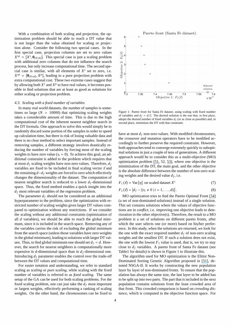
Figure 1: Pareto front for Santa Fe dataset, using scaling with fixed numberof variables anddf = d/2. The desired solution is the one that, in first place,adopts the desired number of fixed variablesdf (or as close as possible) and, insecond place, minimizes the DT with that constraint.

have at mostdf non-zero values. With modified chromosomes,the crossover and mutation operators have to be modified ac-cordingly to further preserve the required constraint. However,both approaches tend to converge extremely quickly to subopti-mal solutions in just a couple of tens of generations. A differentapproach would be to consider this as a multi-objective (MO)optimization problem [51, 52, 53], where one objective is theminimization of the DT, the main goal, and the other objectiveis the absolute difference between the number of non-zero scal-ing weights and the desired valuedf , i.e.

F1(

~s)

= Var[

η]

on scaled datasetXs (7)

F2(

~s)

=∣

∣

∣df − |{si , 0 | i = 1, . . . , d}|∣

∣

∣ . (8)

MO optimization tries to find the Pareto Optimal Front [54](a set of non-dominated solutions) instead of a single solution.This set contains solutions where the values of objective func-tions are inconflict, i.e. improving one objective leads to dete-rioration in the other objective(s). Therefore, the resultto a MOproblem is a set of solutions on different pareto fronts, afterwhich the user selects one (or more) based on his/her prefer-ence. In this study, when the solutions are returned, we lookforthe one with the exact required numberdf of non-zero scalingweights and the smallest DT. If such a solution does not exist,the one with the lowestF2 value is used, that is, we try to stayclose todf variables. A pareto front of Santa Fe dataset (seeTable1 for details) is shown in Figure 1 to illustrate this.

The algorithm used for MO optimization is the Elitist Non-Dominated Sorting Genetic Algorithm proposed in [51], de-noted NSGA-II. It works by constructing the new populationlayer by layer of non-dominated fronts. To ensure that the pop-ulation has always the same size, the last layer to be added hasto be split up into two parts. The part that is included in the nextpopulation contains solutions from the least crowded area ofthat front. This crowded comparison is based oncrowding dis-tance, which is computed in the objective function space. For

4

details see [51]. The overall complexity of NSGA-II isO(hp2),whereh is the number of objectives (in our caseh = 2) andp isthe size of the population.

Fixed scaling is easily extended to include the projectionproblem, in the same manner as explained in Section 4.2 forscaling+ projection. The combination of scaling with a fixednumber of variables and projection will be referred to asfixedscaling+ projection. The projection in this problem is not mod-ified, only the scaling is replaced with the fixed version.

5. Experiments

The experiments were carried out using MATLAB R2009a(TheMathworks Inc., Natick, MA, USA) and its Genetic Algo-rithm and Direct Search Toolbox (GADS). Creation, crossoverand mutation operators are implemented outside of the toolbox.The approximate nearest neighbor search uses a C++ libraryavailable at [55]. The hardware platform used was an Intel Corei7TMTM 920 processor (CPU clock: 4.2 GHz, Cache size: 8MB) with 6 GB of system memory running Windows 7 (64-bit).

The populations are initially created using a specific functionthat assigns a uniform initialization to a percentage of thepop-ulation and the rest can be customized by the user, specifyinghow many of the remaining individuals are initialized randomlyand how many of them are left as zeros. The function is flexiblein the sense that the desired percentage of the initial populationcan be further split into more subsets, each one with a customiz-able percentage of randomly initialized individuals.

The crossover and mutation operators have also been im-plemented as custom functions according to [37]. The muta-tion operator is a pure random uniform function that operatesat a gene level. A relatively high mutation rate (0.1) is usedto enable an effective exploration of the solution space. Thecrossover operator is BLX-α [56], that is specifically devel-oped for a real-coded GA. BLX-α consists in, given two in-dividuals I1 = (i11, i

12, ...i

1d) and I2 = (i21, i

22, ...i

2d) with (i ∈ R),

a new offspringO = (o1, ..., o j, ..., od) can be generated whereo j , j = 1, ..., d is a random value chosen from a uniform dis-tribution within the interval [imin − α · B, imax+ α · B] whereimin = min(i1j , i

2j ), imax = max(i1j , i

2j ), B = imax− imin andα ∈ R.

The selection operator is the binary tournament selection [57].The binary tournament does not require the computation of anyprobability for each individual, saving a considerable amountof operations in each iteration. This can increase computationtime in problems that require large number of individuals inthepopulation.

The population size was fixed to 150 individuals. This valueappears to be a good compromise between performance andcomputational cost for GA-based search applied to similarlysized datasets [37, 58]. After some preliminary tests, the num-ber of generations was fixed to 200 to ensure convergence in allcases. An alternative to this setting could be allowing a dynamicmanagement of the number of generations to be evaluated be-fore stopping the search. Thus, the search would be stopped ifno improvement in the DT has been found forn generations,indicating that the algorithm has converged.

The fitness function of the GA is the DT computed for differ-ent types of problems. In the MO optimization, the DT is one oftwo objective functions. In this paper, we denote with DTS theoptimization of scaling problem using DT, with DTFS the fixedscaling problem, with DTSP-k the problem of scaling+ projec-tion to k dimensions, with DTFS-df the fixed scaling withdf

variables and finally DTFSP-df -k is the problem of fixed scal-ing with df variables plus projection tok dimensions. To em-phasize the goodness of these methods, pure selection (DTSL)has also been included in the comparison.

From previous analysis [37, 58], the best crossover and mu-tation rates for a feature selection application using the GA are0.85 and 0.1 respectively, and an elitism of 10% of the individ-uals was the best compromise.

To sum up, the GA parameters were set as follows:

• Number of averaged runs: 10

• Number of generations evaluated: 200

• Population size: 150

• Population initialization: 20% uniform/ 80% custom. Thecustomized part is further divided into three parts:

– 1/3 with 90% zeros and 10% random genes

– 1/3 with 80% zeros and 20% random genes

– 1/3 with 70% zeros and 30% random genes

• Crossover operator: BLX-α (α = 0.5)

• Selection function: Binary tournament

• Crossover rate: 0.85

• Mutation rate: 0.11

• Elitism: 10%

• Mutation function: Random uniform

The parameterdf was set to⌈d/2⌉ for all datasets throughoutthe experiments.

5.1. Datasets

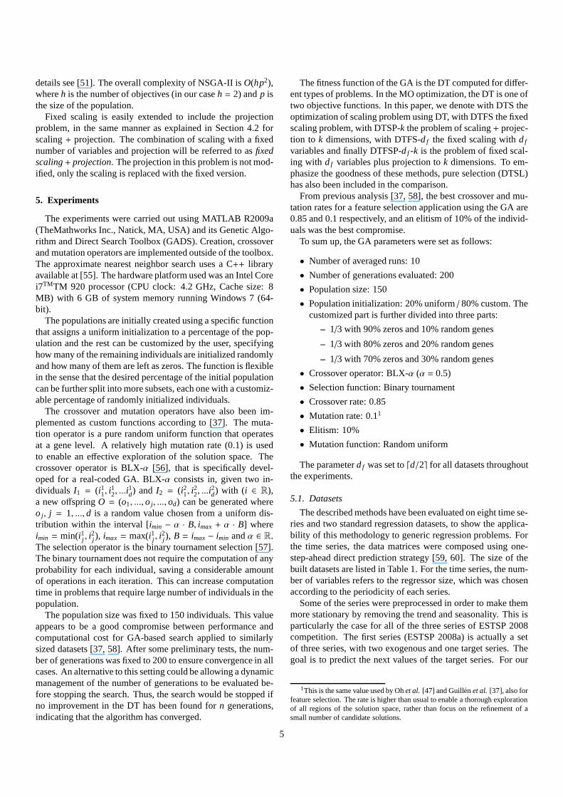
The described methods have been evaluated on eight time se-ries and two standard regression datasets, to show the applica-bility of this methodology to generic regression problems.Forthe time series, the data matrices were composed using one-step-ahead direct prediction strategy [59, 60]. The size ofthebuilt datasets are listed in Table 1. For the time series, thenum-ber of variables refers to the regressor size, which was chosenaccording to the periodicity of each series.

Some of the series were preprocessed in order to make themmore stationary by removing the trend and seasonality. Thisisparticularly the case for all of the three series of ESTSP 2008competition. The first series (ESTSP 2008a) is actually a setof three series, with two exogenous and one target series. Thegoal is to predict the next values of the target series. For our

1This is the same value used by Ohet al. [47] and Guillenet al. [37], also forfeature selection. The rate is higher than usual to enable a thorough explorationof all regions of the solution space, rather than focus on therefinement of asmall number of candidate solutions.

5

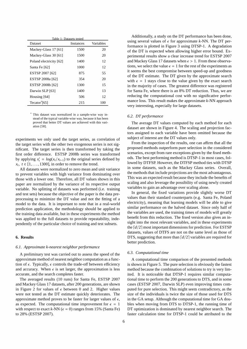
Table 1: Datasets tested

Dataset Instances Variables

Mackey-Glass 17 [61] 1500 20

Mackey-Glass 30 [61] 1500 20

Poland electricity [62] 1400 12

Santa Fe [62] 1000 12

ESTSP 2007 [62] 875 55

ESTSP 2008a [62] 354 20

ESTSP 2008b [62] 1300 15

Darwin SLP [63] 1400 13

Housing [64] 506 12

Tecator*[65] 215 100

* This dataset was normalized in a sample-wise way in-stead of the typical variable-wise way, because it has beenproved that better DT values are achieved with this vari-ation [58].

experiments we only used the target series, as correlation ofthe target series with the other two exogenous series is not sig-nificant. The target series is then transformed by taking thefirst order difference. ESTSP 2008b series was transformedby applyingx′t = log(xt/xt−1) to the original series defined byxt, t ∈ [1, . . . , 1300], in order to remove the trend.

All datasets were normalized to zero mean and unit varianceto prevent variables with high variance from dominating overthose with a lower one. Therefore, all DT values shown in thispaper are normalized by the variance of its respective outputvariable. No splitting of datasets was performed (i.e. trainingand test sets) because the objective of the paper is the data pre-processing to minimize the DT value and not the fitting of amodel to the data. It is important to note that in a real-worldprediction application, the methodology should be appliedtothe training data available, but in these experiments the methodwas applied to the full datasets to provide repeatability, inde-pendently of the particular choice of training and test subsets.

6. Results

6.1. Approximate k-nearest neighbor performance

A preliminary test was carried out to assess the speed of theapproximate method of nearest neighbor computation as a func-tion of ǫ. Typically, ǫ controls the trade-off between efficiencyand accuracy. Whenǫ is set larger, the approximation is lessaccurate, and the search completes faster.

The averaged results (10 runs) for Santa Fe, ESTSP 2007and Mackey Glass 17 datasets, after 200 generations, are shownin Figure 2 for values ofǫ between 0 and 2. Higher valueswere not tested as the DT estimate quickly deteriorates. Theapproximate method proves to be faster for larger values ofǫ,as expected. The computational time improvement forǫ = 1with respect to exactk-NN (ǫ = 0) ranges from 15% (Santa Fe)to 28% (ESTSP 2007).

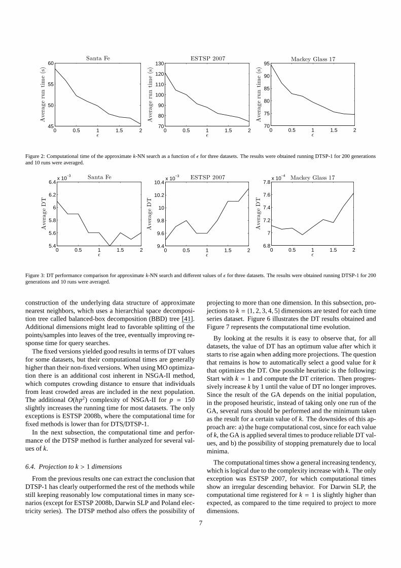
Additionally, a study on the DT performance has been done,using several values ofǫ for approximatek-NN. The DT per-formance is plotted in Figure 3 using DTSP-1. A degradationof the DT is expected when allowing higher error bound. Ex-perimental results show a clear increase trend for ESTSP 2007and Mackey Glass 17 datasets whenǫ > 1. From these observa-tions, we select the valueǫ = 1 for the rest of the experiments asit seems the best compromise between speed-up and goodnessof the DT estimate. The DT given by the approximate searchwith ǫ = 1 stays close to the value given by the exact searchin the majority of cases. The greatest difference was registeredfor Santa Fe, where there is an 8% DT reduction. Thus, we arereducing the computational cost with no significative perfor-mance loss. This result makes the approximatek-NN approachvery interesting, especially for large datasets.

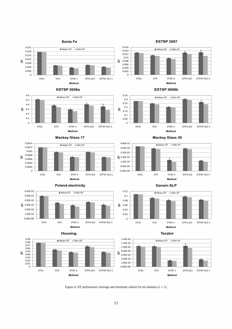
6.2. DT performance

The average DT values computed by each method for eachdataset are shown in Figure 4. The scaling and projection fac-tors assigned to each variable have been omitted because thesubject of interest are the DT values only.

From the inspection of the results, one can affirm that all theproposed methods outperform pure selection in the consideredscenarios, except from rare exceptions given by the fixed meth-ods. The best performing method is DTSP-1 in most cases, fol-lowed by DTFSP. However, the DTFSP method ties with DTSPin some datasets, such as the Mackey Glass series. Overall,the methods that include projections are the most advantageous.This was an expected result because they include the benefitsofscaling and also leverage the possibility of using newly createdvariables to gain an advantage over scaling alone.

In general, the fixed variations provide slightly worse DTvalues than their standard counterparts (e.g. Santa Fe, Polandelectricity), meaning that learning models will be able to givesimilar performance on the halved dataset. Since only half ofthe variables are used, the training times of models will greatlybenefit from this reduction. The fixed version also gives an in-sight into the most relevant variables, and in these experimentsthe⌈d/2⌉most important dimensions for prediction. For ESTSPdatasets, values of DTFS are not on the same level as those ofDTS, suggesting that more than⌈d/2⌉ variables are required forbetter prediction.

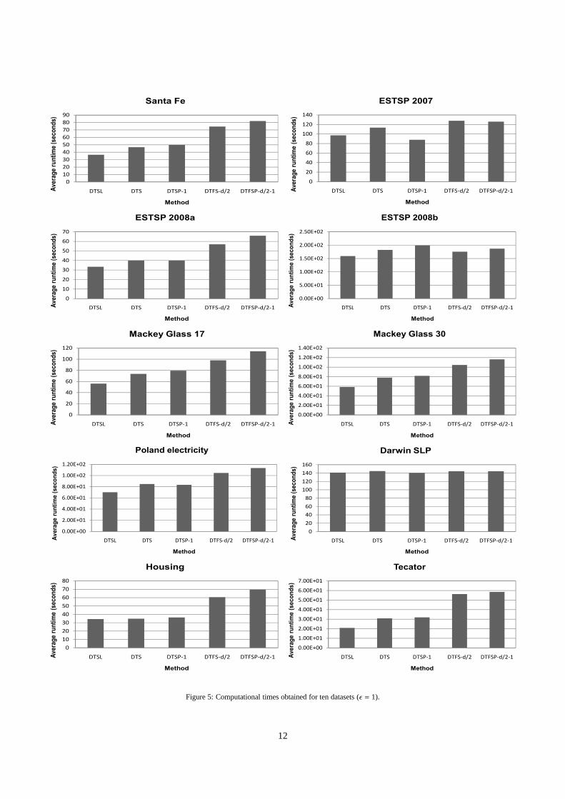
6.3. Computational time

A computational time comparison of the presented methodsis shown in Figure 5. The pure selection is obviously the fastestmethod because the combination of solutions to try is very lim-ited. It is noticeable that DTSP-1 requires similar computa-tional time to perform the 200 generations to DTS, and in somecases (ESTSP 2007, Darwin SLP) even improving times com-puted for pure selection. This might seem contradictory, asthesize of the individuals is twice the size of those used for DTSin the GA setup. Although the computational time for GA dou-bles when moving from DTS to DTSP-1, the running time ofDT optimization is dominated by nearest neighbor search. Thefaster calculation time for DTSP-1 could be attributed to the

6

0 0.5 1 1.5 245

50

55

60

Aver

age

run

tim

e(s

)

ǫ

Santa Fe

0 0.5 1 1.5 270

80

90

100

110

120

130

Aver

age

run

tim

e(s

)

ǫ

ESTSP 2007

0 0.5 1 1.5 270

75

80

85

90

95

Aver

age

run

tim

e(s

)

ǫ

Mackey Glass 17

Figure 2: Computational time of the approximatek-NN search as a function ofǫ for three datasets. The results were obtained running DTSP-1 for 200 generationsand 10 runs were averaged.

0 0.5 1 1.5 25.4

5.6

5.8

6

6.2

6.4x 10

−3

Aver

age

DT

ǫ

Santa Fe

0 0.5 1 1.5 29.4

9.6

9.8

10

10.2

10.4x 10

−3

Aver

age

DT

ǫ

ESTSP 2007

0 0.5 1 1.5 26.8

7

7.2

7.4

7.6

7.8x 10

−4

Aver

age

DT

ǫ

Mackey Glass 17

Figure 3: DT performance comparison for approximatek-NN search and different values ofǫ for three datasets. The results were obtained running DTSP-1 for 200generations and 10 runs were averaged.

construction of the underlying data structure of approximatenearest neighbors, which uses a hierarchial space decomposi-tion tree called balanced-box decomposition (BBD) tree [41].Additional dimensions might lead to favorable splitting ofthepoints/samples into leaves of the tree, eventually improving re-sponse time for query searches.

The fixed versions yielded good results in terms of DT valuesfor some datasets, but their computational times are generallyhigher than their non-fixed versions. When using MO optimiza-tion there is an additional cost inherent in NSGA-II method,which computes crowding distance to ensure that individualsfrom least crowded areas are included in the next population.The additionalO(hp2) complexity of NSGA-II for p = 150slightly increases the running time for most datasets. The onlyexceptions is ESTSP 2008b, where the computational time forfixed methods is lower than for DTS/DTSP-1.

In the next subsection, the computational time and perfor-mance of the DTSP method is further analyzed for several val-ues ofk.

6.4. Projection to k> 1 dimensions

From the previous results one can extract the conclusion thatDTSP-1 has clearly outperformed the rest of the methods whilestill keeping reasonably low computational times in many sce-narios (except for ESTSP 2008b, Darwin SLP and Poland elec-tricity series). The DTSP method also offers the possibility of

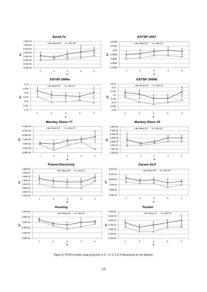
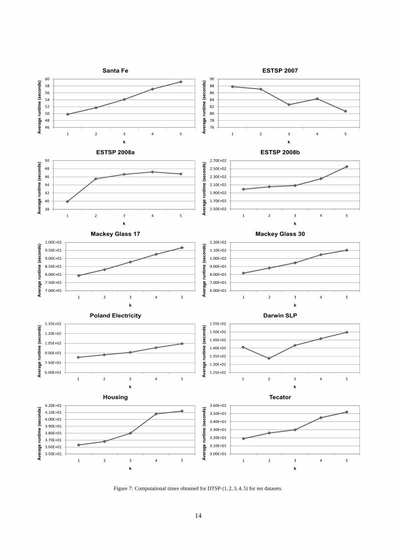
projecting to more than one dimension. In this subsection, pro-jections tok = {1, 2, 3, 4, 5} dimensions are tested for each timeseries dataset. Figure 6 illustrates the DT results obtained andFigure 7 represents the computational time evolution.

By looking at the results it is easy to observe that, for alldatasets, the value of DT has an optimum value after which itstarts to rise again when adding more projections. The questionthat remains is how to automatically select a good value forkthat optimizes the DT. One possible heuristic is the following:Start withk = 1 and compute the DT criterion. Then progres-sively increasek by 1 until the value of DT no longer improves.Since the result of the GA depends on the initial population,in the proposed heuristic, instead of taking only one run of theGA, several runs should be performed and the minimum takenas the result for a certain value ofk. The downsides of this ap-proach are: a) the huge computational cost, since for each valueof k, the GA is applied several times to produce reliable DT val-ues, and b) the possibility of stopping prematurely due to localminima.

The computational times show a general increasing tendency,which is logical due to the complexity increase withk. The onlyexception was ESTSP 2007, for which computational timesshow an irregular descending behavior. For Darwin SLP, thecomputational time registered fork = 1 is slightly higher thanexpected, as compared to the time required to project to moredimensions.

7

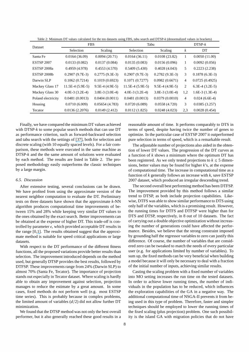
Table 2: Minimum DT values calculated for the ten datasets using FBS, tabu search and DTSP-k (denormalized values in brackets)

DatasetFBS Tabu DTSP-k

Selection Scaling Selection Scaling k DT

Santa Fe 0.0164 (36.09) 0.0094 (20.71) 0.0164 (36.11) 0.0108 (23.82) 1 0.0050 (11.00)

ESTSP 2007 0.0133 (0.082) 0.0137 (0.084) 0.0135 (0.083) 0.0156 (0.096) 1 0.0092 (0.056)

ESTSP 2008a 0.4959 (4.978) 0.4553 (4.570) 0.5409 (5.430) 0.4028 (4.043) 5 0.2223 (2.238)

ESTSP 2008b 0.2907 (9.7E-3) 0.2775 (9.3E-3) 0.2907 (9.7E-3) 0.2782 (9.3E-3) 3 0.1878 (6.3E-3)

Darwin SLP 0.1062 (0.7214) 0.1019 (0.6923) 0.1071 (0.7277)0.0982 (0.6671) 4 0.0725 (0.4925)

Mackey Glass 17 11.5E-4 (5.9E-5) 9.5E-4 (4.9E-5) 11.5E-4 (5.9E-5) 9.5E-4 (4.9E-5) 2 6.3E-4 (3.2E-5)

Mackey Glass 30 4.0E-3 (3.2E-4) 3.8E-3 (3.0E-4) 4.0E-3 (3.2E-4) 3.8E-3 (3.0E-4) 1,2 1.6E-3 (1.3E-4)

Poland electricity 0.0481 (0.0013) 0.0404 (0.0011) 0.0481(0.0013) 0.0379 (0.0010) 4 0.024 (6.6E-4)

Housing 0.0710 (6.009) 0.05654 (4.783) 0.0720 (6.089) 0.0558 (4.720) 3 0.0385 (3.257)

Tecator 0.0136 (2.2076) 0.0149 (2.412) 0.0112 (1.825) 0.0248 (4.023) 2,3 0.0028 (0.454)

Finally, we have compared the minimum DT values achievedwith DTSP-k to some popular search methods that can use DTas performance criterion, such as forward-backward selectionand tabu search with the settings of [37], both for selectionanddiscrete scaling (with 10 equally spaced levels). For a faircom-parison, these methods were executed in the same machine asDTSP-k and the the same amount of solutions were evaluatedby each method. The results are listed in Table 2. The pro-posed methodology easily outperforms the classic techniquesby a large margin.

6.5. Discussion

After extensive testing, several conclusions can be drawn.We have profited from using the approximate version of thenearest neighbor computation to evaluate the DT. Preliminarytests on three datasets have shown that the approximatek-NNalgorithm produces computational time improvements of be-tween 15% and 28% while keeping very similar DT values tothe ones obtained by the exact search. Better improvements canbe obtained at the expense of higher DT. This trade-off is con-trolled by parameterǫ, which provided acceptable DT results inthe range [0,1]. The results obtained suggest that the approxi-mate method is suitable for speed critical applications or largedatasets.

With respect to the DT performance of the different fitnessfunctions, all the proposed variations provide better results thanselection. The improvement introduced depends on the methodused, but generally DTSP provides the best results, followed byDTFSP. These improvements range from 24% (Darwin SLP) toalmost 70% (Santa Fe, Tecator). The importance of projectionstands out especially in Tecator dataset. Where scaling is hardlyable to obtain any improvement against selection, projectionmanages to reduce the estimate by a great amount. In somecases, fixed methods do not perform well (e.g. most ESTSPtime series). This is probably because in complex problems,the limited amount of variables (d/2) did not allow further DTminimization.

We found that the DTSP method was not only the best overallperformer, but it also generally reached these good resultsin a

reasonable amount of time. It performs comparably to DTS interms of speed, despite having twice the number of genes tooptimize. In the particular case of ESTSP 2007 it outperformedpure selection in terms of speed, which is a remarkable result.

The adjustable number of projections also aided in the obten-tion of lower DT values. The progression of the DT curves asa function ofk shows a minimum where the optimum DT hasbeen registered. As we only tested projections tok ≤ 5 dimen-sions, better values may be found for higherk’s, at the expenseof computational time. The increase in computational time as afunction ofk generally follows an increase withk, save ESTSP2007 dataset, which produced an irregular descending trend.

The second overall best performing method has been DTFSP.The improvement provided by this method follows a similartrend to DTSP, as both include projection capabilities. Like-wise, DTFS was able to show similar performance to DTS usingonly half of the variables, which is a promising result. However,the running times for DTFS and DTFSP were higher than forDTS and DTSP, respectively, in 8 out of 10 datasets. The factof carrying out a double objective optimization without increas-ing the number of generations could have affected the perfor-mance. Besides, we believe that the strong constraint imposedby grounding half the regressor variables to zero can justify thisdifference. Of course, the number of variables that are consid-ered zero can be tweaked to match the needs of every particularuser (e.g. for applications limited by number of variables). Tosum up, the fixed methods can be very beneficial when buildinga model because it will only be necessary to deal with a fractionof the initial number of inputs, achieving similar results.

Casting the scaling problem with a fixed number of variablesinto MO setting increases the run time on the tested datasets.In order to achieve lower running times, the number of indi-viduals in the population has to be reduced, which influencesthe exploration capabilities of the GA in a negative way. Theadditional computational time of NSGA-II prevents it from be-ing used in this type of problem. Therefore, faster and simplertechniques should be employed to lower the running times ofthe fixed scaling (plus projection) problem. One such possibil-ity is the island GA with migration policies that do not have

8

such high complexity.

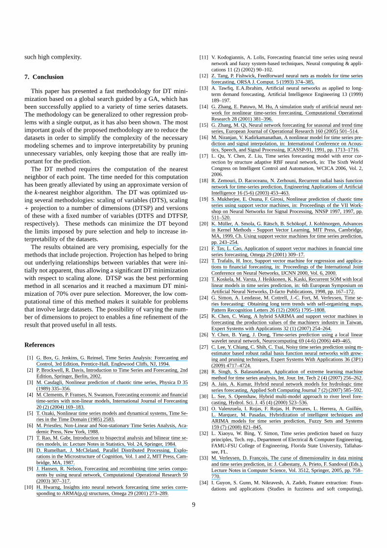
7. Conclusion

This paper has presented a fast methodology for DT mini-mization based on a global search guided by a GA, which hasbeen successfully applied to a variety of time series datasets.The methodology can be generalized to other regression prob-lems with a single output, as it has also been shown. The mostimportant goals of the proposed methodology are to reduce thedatasets in order to simplify the complexity of the necessarymodeling schemes and to improve interpretability by pruningunnecessary variables, only keeping those that are really im-portant for the prediction.

The DT method requires the computation of the nearestneighbor of each point. The time needed for this computationhas been greatly alleviated by using an approximate versionofthe k-nearest neighbor algorithm. The DT was optimized us-ing several methodologies: scaling of variables (DTS), scaling+ projection to a number of dimensions (DTSP) and versionsof these with a fixed number of variables (DTFS and DTFSP,respectively). These methods can minimize the DT beyondthe limits imposed by pure selection and help to increase in-terpretability of the datasets.

The results obtained are very promising, especially for themethods that include projection. Projection has helped to bringout underlying relationships between variables that were ini-tially not apparent, thus allowing a significant DT minimizationwith respect to scaling alone. DTSP was the best performingmethod in all scenarios and it reached a maximum DT mini-mization of 70% over pure selection. Moreover, the low com-putational time of this method makes it suitable for problemsthat involve large datasets. The possibility of varying thenum-ber of dimensions to project to enables a fine refinement of theresult that proved useful in all tests.

References

[1] G. Box, G. Jenkins, G. Reinsel, Time Series Analysis: Forecasting andControl, 3rd Edition, Prentice-Hall, Englewood Cliffs, NJ, 1994.

[2] P. Brockwell, R. Davis, Introduction to Time Series and Forecasting, 2ndEdition, Springer, Berlin, 2002.

[3] M. Casdagli, Nonlinear prediction of chaotic time series, Physica D 35(1989) 335–356.

[4] M. Clements, P. Franses, N. Swanson, Forecasting economic and financialtime-series with non-linear models, International Journal of Forecasting20 (2) (2004) 169–183.

[5] T. Ozaki, Nonlinear time series models and dynamical systems, Time Se-ries in the Time Domain (1985) 2583.

[6] M. Priestley, Non-Linear and Non-stationary Time Series Analysis, Aca-demic Press, New York, 1988.

[7] T. Rao, M. Gabr, Introduction to bispectral analysis andbilinear time se-ries models, in: Lecture Notes in Statistics, Vol. 24, Springer, 1984.

[8] D. Rumelhart, J. McCleland, Parallel Distributed Processing, Explo-rations in the Microstructure of Cognition, Vol. 1 and 2, MITPress, Cam-bridge, MA, 1987.

[9] J. Hansen, R. Nelson, Forecasting and recombining time series compo-nents by using neural network, Computational Operational Research 50(2003) 307–317.

[10] H. Hwarng, Insights into neural network forecasting time series corre-sponding to ARMA(p,q) structures, Omega 29 (2001) 273–289.

[11] V. Kodogiannis, A. Lolis, Forecasting financial time series using neuralnetwork and fuzzy system-based techniques, Neural computing & appli-cations 11 (2) (2002) 90–102.

[12] Z. Tang, P. Fishwick, Feedforward neural nets as modelsfor time seriesforecasting, ORSA J. Comput. 5 (1993) 374–385.

[13] A. Tawfiq, E.A.Ibrahim, Artificial neural networks as applied to long-term demand forecasting, Artificial Intelligence Engineering 13 (1999)189–197.

[14] G. Zhang, E. Patuwo, M. Hu, A simulation study of artificial neural net-work for nonlinear time-series forecasting, Computational OperationalResearch 28 (2001) 381–396.

[15] G. Zhang, M. Qi, Neural network forecasting for seasonal and trend timeseries, European Journal of Operational Research 160 (2005) 501–514.

[16] M. Niranjan, V. Kadirkamanathan, A nonlinear model fortime series pre-diction and signal interpolation, in: International Conference on Acous-tics, Speech, and Signal Processing, ICASSP-91, 1991, pp. 1713–1716.

[17] L. Qu, Y. Chen, Z. Liu, Time series forecasting model with error cor-rection by structure adaptive RBF neural network, in: The Sixth WorldCongress on Intelligent Control and Automation, WCICA 2006, Vol. 2,2006.

[18] R. Zemouri, D. Racoceanu, N. Zerhouni, Recurrent radial basis functionnetwork for time-series prediction, Engineering Applications of ArtificialIntelligence 16 (5-6) (2003) 453–463.

[19] S. Mukherjee, E. Osuna, F. Girosi, Nonlinear prediction of chaotic timeseries using support vector machines, in: Proceedings of the VII Work-shop on Neural Networks for Signal Processing, NNSP 1997, 1997, pp.511–520.

[20] K. Muller, A. Smola, G. Ratsch, B. Schokopf, J. Kohlmorgen, Advancesin Kernel Methods - Support Vector Learning, MIT Press, Cambridge,MA, 1999, Ch. Using support vector machines for time series prediction,pp. 243–254.

[21] F. Tay, L. Cao, Application of support vector machines in financial timeseries forecasting, Omega 29 (2001) 309–17.

[22] T. Trafalis, H. Ince, Support vector machine for regression and applica-tions to financial forecasting, in: Proceedings of the International JointConference on Neural Networks, IJCNN 2000, Vol. 6, 2000.

[23] T. Koskela, M. Varsta, J. Heikkonen, K. Kaski, Recurrent SOM with locallinear models in time series prediction, in: 6th European Symposium onArtificial Neural Networks, D-facto Publications, 1998, pp. 167–172.

[24] G. Simon, A. Lendasse, M. Cottrell, J.-C. Fort, M. Verleysen, Time se-ries forecasting: Obtaining long term trends with self-organizing maps,Pattern Recognition Letters 26 (12) (2005) 1795–1808.

[25] K. Chen, C. Wang, A hybrid SARIMA and support vector machines inforecasting the production values of the machinery industry in Taiwan,Expert Systems with Applications 32 (1) (2007) 254–264.

[26] Y. Chen, B. Yang, J. Dong, Time-series prediction usinga local linearwavelet neural network, Neurocomputing 69 (4-6) (2006) 449–465.

[27] C. Lee, Y. Chiang, C. Shih, C. Tsai, Noisy time series prediction using m-estimator based robust radial basis function neural networks with grow-ing and pruning techniques, Expert Systems With Applications 36 (3P1)(2009) 4717–4724.

[28] R. Singh, S. Balasundaram, Application of extreme learning machinemethod for time series analysis, Int. Jour. Int. Tech 2 (4) (2007) 256–262.

[29] A. Jain, A. Kumar, Hybrid neural network models for hydrologic timeseries forecasting, Applied Soft Computing Journal 7 (2) (2007) 585–592.

[30] L. See, S. Openshaw, Hybrid multi-model approach to river level fore-casting, Hydrol. Sci. J. 45 (4) (2000) 523–536.

[31] O. Valenzuela, I. Rojas, F. Rojas, H. Pomares, L. Herrera, A. Guillen,L. Marquez, M. Pasadas, Hybridization of intelligent techniques andARIMA models for time series prediction, Fuzzy Sets and Systems159 (7) (2008) 821–845.

[32] L. Xiaoyu, W. Bing, Y. Simon, Time series prediction based on fuzzyprinciples, Tech. rep., Department of Electrical & Computer Engineering,FAMU-FSU College of Engineering, Florida State University, Tallahas-see, FL.

[33] M. Verleysen, D. Francois, The curse of dimensionality in data miningand time series prediction, in: J. Cabestany, A. Prieto, F. Sandoval (Eds.),Lecture Notes in Computer Science, Vol. 3512, Springer, 2005, pp. 758–770.

[34] I. Guyon, S. Gunn, M. Nikravesh, A. Zadeh, Feature extraction: Foun-dations and applications (Studies in fuzziness and soft computing),

9

Springer-Verlag New York, Secaucus, NJ, USA, 2006.[35] E. Eirola, E. Liitiainen, A. Lendasse, F. Corona, M. Verleysen, Using

the delta test for variable selection, in: Proc. of ESANN 2008, EuropeanSymposium on Artificial Neural Networks, Bruges, Belgium, 2008, pp.25–30.

[36] Q. Yu, E. Severin, A. Lendasse, A global methodology for variable se-lection: application to financial modeling, in: Proc. of MASHS 2007,ENST-Bretagne, France, 2007.

[37] A. Guillen, D. Sovilj, F. Mateo, I. Rojas, A. Lendasse,Minimizing thedelta test for variable selection in regression problems, Int. J. of HighPerformance Systems Architecture 1 (4) (2008) 269–281.

[38] F. Mateo, A. Lendasse, A variable selection approach based on the deltatest for extreme learning machine models, in: Proc. of ESTSP2008, Eu-ropean Symposium on Time Series Prediction, Porvoo, Finland, 2008, pp.57–66.

[39] D. Sovilj, A. Sorjamaa, Y. Miche, Tabu search with deltatest for timeseries prediction using OP-KNN, in: Proc. of ESTSP 2008, EuropeanSymposium on Time Series Prediction, Porvoo, Finland, 2008, pp. 187–196.

[40] J. Holland, Adaptation in natural and artificial systems, University ofMichigan Press, 1975.

[41] S. Arya, D. Mount, N. Netanyahu, R. Silverman, A. Wu, An optimalalgorithm for approximate nearest neighbor searching fixeddimensions,Journal of the ACM (JACM) 45 (6) (1998) 891–923.

[42] H. Pi, C. Peterson, Finding the embedding dimension andvariable depen-dencies in time series, Neural Computation 6 (3) (1994) 509–520.

[43] E. Liitiainen, F. Corona, A. Lendasse, On nonparametric residual varianceestimation, Neural Processing Letters 28 (3) (2008) 155–167.

[44] A. Jones, New tools in non-linear modelling and prediction, Computa-tional Management Science 1 (2) (2004) 109–149.

[45] J. Friedman, J. Bentley, R. Finkel, An algorithm for finding best matchesin logarithmic expected time, ACM Transactions on Mathematical Soft-ware (TOMS) 3 (3) (1977) 209–226.

[46] I.-S. Oh, J.-S. Lee, B.-R. Moon, Local search-embeddedgenetic algo-rithms for feature selection, Proc. of the 16th Int. Conference on PatternRecognition 2 (2002) 148–151.

[47] I.-S. Oh, J.-S. Lee, B.-R. Moon, Hybrid genetic algorithms for feature se-lection, IEEE Trans. on Pattern Analysis and Machine Intelligence 26 (11)(2004) 1424–1437.

[48] W. Punch, E. Goodman, M. Pei, L. Chia-Shun, P. Hovland, R. Enbody,Further research on feature selection and classification using genetic al-gorithms, in: S. Forrest (Ed.), Proc. of the Fifth Int. Conf.on GeneticAlgorithms, Morgan Kaufmann, San Mateo, CA, 1993, pp. 557–564.

[49] M. Raymer, W. Punch, E. Goodman, L. Kuhn, A. Jain, Dimensionalityreduction using genetic algorithms, IEEE Trans. on Evolutionary Com-putation 4 (2) (2000) 164–171.

[50] Y. Saeys, I. Inza, P. Larranaga, A review of feature selection techniquesin bioinformatics, Bioinformatics 23 (19) (2007) 2507–2517.

[51] K. Deb, S. Agrawal, A. Pratap, T. Meyarivan, A fast elitist non-dominatedsorting genetic algorithm for multi-objective optimization: NSGA-II,Springer, 2000, pp. 849–858.

[52] K. Miettinen, Nonlinear Multiobjective Optimization, Vol. 12 of Interna-tional Series in Operations Research and Management Science, KluwerAcademic Publishers, Dordrecht, 1999.

[53] R. Steuer, Multiple Criteria Optimization : Theory, Computation, andApplication, Wiley, New York, Toronto, 1986.

[54] K. Deb, Multi-Objective Optimization Using Evolutionary Algorithms,Wiley, Chichester, UK, 2001.

[55] http://www.cs.umd.edu/∼mount/ANN/.[56] L. Eshelman, J. Schaffer, Real-coded genetic algorithms and interval

schemata, in: L. Darrell Whitley (Ed.), Foundation of Genetic Algorithms2, Morgan-Kauffman Publishers, Inc., 1993, pp. 187–202.

[57] D. Goldberg, Genetic algorithms in search, optimization and machinelearning, Addison Wesley, 1989.

[58] F. Mateo, D. Sovilj, R. Gadea, A. Lendasse, RCGA-S/RCGA-SP methodsto minimize the delta test for regression tasks, in: J. C. et al. (Ed.), LectureNotes in Computer Science, Vol. 5517, Springer, 2009, pp. 359–366.

[59] Y. Ji, J. Hao, N. Reyhani, A. Lendasse, Direct and recursive predictionof time series using mutual information selection, in: International Work-Conference on Artificial Neural Networks, IWANN, Springer,2005, pp.8–10.

[60] A. Sorjamaa, J. Hao, N. Reyhani, Y. Ji, A. Lendasse, Methodology forlong-term prediction of time series, Neurocomputing 70 (16-18) (2007)2861–2869.

[61] http://www.cse.ogi.edu/∼ericwan/data.html.[62] http://www.cis.hut.fi/projects/tsp/index.php?page=

timeseries.[63] http://www.stat.duke.edu/∼mw/data-sets/ts data/

darwin.slp.[64] http://archive.ics.uci.edu/ml/data sets/Housing.[65] http://lib.stat.cmu.edu/data sets/tecator.

Fernando Mateo was born in Valencia, Spain,in 1981. He obtained his M.Sc. in Telecom-munication Engineering in 2005 from the Univer-sidad Politecnica de Valencia, Spain. Currently,he is a researcher pursuing his Ph.D. at the In-stitute of Applications of Information Technologyand Advanced Communications, at the same Uni-versity. In 2007 and 2008 he also collaboratedwith the Computer Science and Information Labo-ratory at Helsinki University of Technology, Fin-land. His research is related to machine learn-ing methods and applications like position estima-

tion in positron emission tomography detectors, prediction of contaminantsin food and variable selection techniques for high-dimensional problems.

Dusan Sovilj obtained his B.Sc. in 2006 fromUniversity of Novi Sad, Serbia. He is pursuing aMaster degree at Helsinki University of Technol-ogy in Finland, and at the same time working atthe Time Series Prediction and ChemoinformaticsGroup at the same University. His main topics ofresearch are time series prediction and variable se-lection in regression problems. He is also inter-ested in artificial intelligence in computer games.

Rafael Gadeareceived the M.Sc. and Ph.D. de-grees from the Universidad Politecnica de Valen-cia, Spain, in 1990 and 2000, respectively. Since1992 he has been a lecturer of the Departmentof Electronics at the Universidad Politecnica deValencia. Currently, he is assistant professor atTelecommunications Engineering School of theUniversidad Politecnica de Valencia, Spain. Hisareas of research interest include hardware de-scription languages, design of FPGA-based sys-tems and design of neural networks and cellular

automata.

10

�����

�����

�����

�����

�����

����

�����

DT

Santa Fe

�� ��� � ���

�

�����

�����

�����

�����

�����

����

�����

���� ��� ������ �������� �����������

DT

Method

Santa Fe

�� ��� � ���

�����

�����

�����

����

�����

�����

�����

DT

ESTSP 2007

��� � ���� �

�

�����

�����

�����

�����

����

�����

�����

�����

��� �� ����� ������� ����������

DT

Method

ESTSP 2007

��� � ���� �

���

���

���

���

���

���

DT

ESTSP 2008a

�� �� �� ��

�

���

���

���

���

���

���

���� ��� ������ �������� �����������

DT

Method

ESTSP 2008a

�� �� �� ��

����

���

����

���

����

���

����

DT

ESTSP 2008b

���� ����

�

����

���

����

���

����

���

����

� �� � � � ���� � ������ � ���������

DT

Method

ESTSP 2008b

���� ����

������

������

������

������

�����

������

������

DT

Mackey Glass 17

��� � ���� �

�

������

������

������

������

�����

������

������

��� �� ����� ������� ����������

DT

Method

Mackey Glass 17

��� � ���� �

��������

�������

������

�����

�������

�������

DT

Mackey Glass 30

�� ���� ������

��������

��������

�������

������

�����

�������

�������

���� ��� ������ ������� ����������

DT

Method

Mackey Glass 30

�� ���� ������

��������

��������

��������

��������

�������

�������

DT

Poland electricity

�� ���� ������

��������

��������

��������

��������

��������

�������

�������

���� ��� ������ �������� �����������

DT

Method

Poland electricity

�� ���� ������

����

����

����

����

���

����

DT

Darwin SLP

��� � ���� �

�

����

����

����

����

���

����

��� �� ����� ������� ����������

DT

Method

Darwin SLP

��� � ���� �

����

����

����

����

����

����

���

���

DT

Housing

�� ���� ������

�

����

����

����

����

����

����

����

���

���

���� ��� ������ �������� �����������

DT

Method

Housing

�� ���� ������

��������

��������

��������

������

�����

������

DT

Tecator

�� ���� ������

��������

�������

��������

��������

��������

������

�����

������

���� ��� ����� ������� ���������

DT

Method

Tecator

�� ���� ������

Figure 4: DT performance (average and minimum values) for ten datasets (ǫ = 1).

11

��

��

��

��

��

��

��

�

run

tim

e�s

ec

on

ds�

Santa Fe

�

�

��

��

��

��

��

��

��

�

�� � �� �� �� ��� ���� ��� ������Ave

rag

eru

nti

me�s

ec

on

ds�

Method

Santa Fe

��

��

��

���

���

���

Ave

rag

e r

un

tim

e (

se

co

nd

s)

ESTSP 2007

�

��

��

��

��

���

���

���

�� �� ����� �� ���� �� �������Ave

rag

e r

un

tim

e (

se

co

nd

s)

Method

ESTSP 2007

��

��

��

��

��

��

��

Av

era

ge

ru

nti

me

(s

eco

nd

s)

ESTSP 2008a

�

��

��

��

��

��

��

��

�� � � �� ������ �� ������Av

era

ge

ru

nti

me

(s

eco

nd

s)

Method

ESTSP 2008a

��������

��������

��������

��������

��������

Av

era

ge

ru

nti

me (

se

co

nd

s)

ESTSP 2008b

��������

��������

��������

��������

��������

��������

�� � �� � �� ��� ��� ��� �Av

era

ge

ru

nti

me (

se

co

nd

s)

Method

ESTSP 2008b

��

��

��

��

���

���

Ave

rag

e r

un

tim

e (

se

co

nd

s)

Mackey Glass 17

�

��

��

��

��

���

���

�� �� ����� �� ���� �� �������Ave

rag

e r

un

tim

e (

se

co

nd

s)

Method

Mackey Glass 17

��������

��������

��������

�������

������

�������

Ave

rag

e r

un

tim

e (

se

co

nd

s)

Mackey Glass 30

��������

�������

��������

��������

��������

�������

������

�������

�� �� ����� ������ ���������Ave

rag

e r

un

tim

e (

se

co

nd

s)

Method

Mackey Glass 30

��������

��������

��������

�������

��������

��������

Av

era

ge r

un

tim

e (

se

co

nd

s)

Poland electricity

��������

��������

��������

��������

�������

��������

��������

�� �� ����� ������� ����������Av

era

ge r

un

tim

e (

se

co

nd

s)

Method

Poland electricity

��

��

��

���

���

���

���

Av

era

ge

ru

nti

me (

se

co

nd

s)

Darwin SLP

�

��

��

��

��

���

���

���

���

�� �� ����� �� ���� �� �������Av

era

ge

ru

nti

me (

se

co

nd

s)

Method

Darwin SLP

��

��

��

��

��

��

��

Ave

rag

e r

un

tim

e (

se

co

nd

s)

Housing

�

�

��

��

��

��

��

��

��

�� �� ���� ������� ���������Ave

rag

e r

un

tim

e (

se

co

nd

s)

Method

Housing

��������

��������

��������

�������

�������

��������

Ave

rag

e r

un

tim

e (

se

co

nd

s)

Tecator

��������

��������

��������

��������

��������

�������

�������

��������

� �� � � � ���� � ������ � ���������Ave

rag

e r

un

tim

e (

se

co

nd

s)

Method

Tecator

Figure 5: Computational times obtained for ten datasets (ǫ = 1).

12

��������

��������

��������

��������

��������

DT

Santa Fe

�� �� �� ��

��������

��������

��������

��������

��������

��������

��������

��������

� � � � �

DT

k

Santa Fe

�� �� �� ��

������

����

������

������

DT

ESTSP 2007

��� � ���� �

������

������

������

������

����

������

������

� � � � �

DT

k

ESTSP 2007

��� � ���� �

�����

����

�����

����

DT

ESTSP 2008a

���� ����

����

�����

����

�����

����

�����

����

� � � � �

DT

k

ESTSP 2008a

���� ����

�����

���

�����

����

�����

DT

ESTSP 2008b

���� ����

����

�����

����

�����

���

�����

����

�����

� � � � �

DT

k

ESTSP 2008b

���� ����

��������

��������

��������

�������

DT

Mackey Glass 17

�� ��� � ���

��������

��������

��������

��������

��������

��������

�������

� � � � �

DT

k

Mackey Glass 17

�� ��� � ���

��������

��������

��������

�������

�������

DT

Mackey Glass 30

�� ���� ������

��������

�������

�������

��������

��������

��������

�������

�������

� � � �

DT

k

Mackey Glass 30

�� ���� ������

��������

��������

��������

��������

�������

DT

Poland Electricity

�� ��� � ���

��������

��������

�������

��������

��������

��������

��������

�������

� � � �

DT

k

Poland Electricity

�� ��� � ���

��������

��������

��������

�������

DT

Darwin SLP

�� ��� � ���

��������

��������

��������

��������

��������

�������

� � � � �

DT

k

Darwin SLP

�� ��� � ���

��������

��������

��������

��������

DT

Housing

��� � ���� �

��������

��������

��������

��������

��������

��������

� � � � �

DT

k

Housing

��� � ���� �

��������

��������

��������

��������

DT

Tecator

�� �� �� ��

��������

��������

��������

��������

��������

��������

��������

� � � � �

DT

k

Tecator

�� �� �� ��

Figure 6: DTSP-k results using projection tok = {1, 2, 3, 4,5} dimensions for ten datasets.

13

��

��

��

��

��

��

Ave

rag

e r

un

tim

e (

se

co

nd

s)

Santa Fe

��

��

��

��

��

��

��

��

� � � � �

Ave

rag

e r

un

tim

e (

se

co

nd

s)

k

Santa Fe

��

��

��

��

��

��

Ave

rag

e r

un

tim

e (

se

co

nd

s)

ESTSP 2007

��

��

��

��

��

��

��

��

� � �

Ave

rag

e r

un

tim

e (

se

co

nd

s)

k

ESTSP 2007

��

��

��

��

��

Av

era

ge r

un

tim

e (

se

co

nd

s)

ESTSP 2008a

��

��

��

��

��

��

��

� � � � �

Av

era

ge r

un

tim

e (

se

co

nd

s)

k

ESTSP 2008a

��������

��������

��������

�������

�������

Ave

rag

e r

un

tim

e (

se

co

nd

s)

ESTSP 2008b

�������

�������

��������

��������

��������

�������

�������

� � � �

Ave

rag

e r

un

tim

e (

se

co

nd

s)

k

ESTSP 2008b

��������

��������

��������

��������

�������

Ave

rag

e r

un

tim

e (

se

co

nd

s)

Mackey Glass 17

�������

�������

��������

��������

��������

��������

�������

� � � �

Ave

rag

e r

un

tim

e (

se

co

nd

s)

k

Mackey Glass 17

��������

��������

��������

��������

��������

Ave

rag

e r

un

tim

e (

se

co

nd

s)

Mackey Glass 30

�������

�������

��������

��������

��������

��������

��������

� � � �

Ave

rag

e r

un

tim

e (

se

co

nd

s)

k

Mackey Glass 30

��������

��������

��������

�������

Av

era

ge

ru

nti

me

(s

ec

on

ds

)

Poland Electricity

�������

��������

��������

��������

��������

�������

� � � �

Av

era

ge

ru

nti

me

(s

ec

on

ds

)

k

Poland Electricity

��������

�������

�������

��������

��������

Av

era

ge r

un

tim

e (

se

co

nd

s)

Darwin SLP

��������

��������

��������

�������

�������

��������

��������

� � � �

Av

era

ge r

un

tim

e (

se

co

nd

s)

k

Darwin SLP

��������

��������

�������

�������

�������

�������

Ave

rag

e r

un

tim

e (

se

co

nd

s)

Housing

��������

�� �����

��������

��������

�������

�������

�������

�������

� � � �

Ave

rag

e r

un

tim

e (

se

co

nd

s)

k

Housing

��������

��������

��������

�������

�������

Ave

rag

e r

un

tim

e (

se

co

nd

s)

Tecator

��������

��������

��������

��������

��������

�������

�������

� � � �

Ave

rag

e r

un

tim

e (

se

co

nd

s)

k

Tecator

Figure 7: Computational times obtained for DTSP-{1,2, 3, 4, 5} for ten datasets.

14