Design, Evaluation and Application of ApproximateArithmetic Circuits

by

Honglan Jiang

A thesis submitted in partial fulfillment of the requirements for the degree of

Doctor of Philosophy

in

Integrated Circuits and Systems

Department of Electrical and Computer Engineering

University of Alberta

© Honglan Jiang, 2018

Abstract

As very important modules in a processor, arithmetic circuits often play a pivotal role in

determining the performance and power dissipation of a demanding computation. The

demand for higher speed and power efficiency, as well as the desirability for error

resilience in many applications (e.g., multimedia, recognition and data analytics) has

driven the development of approximate arithmetic circuit design. In this dissertation,

approximate arithmetic circuits are evaluated, several fundamental approximate circuits

are devised, and a high-performance and energy-efficient approximate adaptive filter is

proposed using approximate distributed arithmetic (DA) circuits.

Existing approximate arithmetic circuits in the literature are first reviewed, evaluated

and compared to guide the selection of a suitable approximate design for a specific

application with designated purposes. A low-power approximate radix-8 Booth multiplier

using an approximate recoding adder is then proposed for signed multiplication.

Compared with an accurate multiplier, the proposed approximate design saves as much as

44% in power and 43% in area with a mean relative error distance (MRED) of 0.43%.

Compared with the other approximate Booth multipliers, the proposed design has the

lowest power-delay product while providing a moderate accuracy. Moreover, an adaptive

approximation approach is proposed for the design of a divider and a square root (SQR)

circuit. In this design, the division/SQR is computed using a reduced-width divider/SQR

circuit and a shifter by adaptively pruning the input bits. The synthesis results show that

the proposed approximate divider with an MRED of 6.6% achieves more than 60%

improvements in speed and power dissipation compared with an accurate design. The

ii

proposed divider is more accurate than other approximate dividers when a similar

power-delay product is considered. By changing the width of the reduced-width SQR

circuit, the approximate SQR circuit is 22.69% to 74.54% faster, and saves 30.75% to

79.34% in power with an MRED from 0.7% to 8.0% compared with an accurate design.

Compared to other approximate designs, the proposed approximate divider and SQR

circuit designs perform better in image processing applications.

The superior control capability of the cerebellum has motivated extensive interest in

the development of computational cerebellar models. Many models have been applied to

motor control and image stabilization in robots. Often computationally complex,

cerebellar models have rarely been implemented in dedicated hardware. In this

dissertation, a fixed-point finite impulse response adaptive filter is proposed using

approximate DA circuits. This design can be used in general digital signal processing

applications as well as in control systems as an adaptive filter-based cerebellar model. In

this design, the radix-8 Booth algorithm is used to reduce the number of partial products

in the DA architecture, and the partial products are approximately generated by truncating

the input data with error compensation, accumulated by using an approximate Wallace

tree. At a similar accuracy, the proposed design attains on average a 55% reduction in

energy per operation and a 2.2× increase in throughput per area compared with an

accurate design. A saccadic system using the proposed approximate adaptive filter-based

cerebellar model achieves a similar retinal slip as using an accurate filter. These results are

promising for the large-scale integration of approximate circuits into high-performance

and energy-efficient systems for error-resilient applications.

iii

Preface

This dissertation presents an original work in the field of approximate computing by

Honglan Jiang.

In Chapter 2, current approximate arithmetic circuits including adders, multipliers and

dividers are first reviewed, classified and comparatively evaluated. This work has been

published as H. Jiang, C. Liu, L. Liu, F. Lombardi, and J. Han, "A review, classification,

and comparative evaluation of approximate arithmetic circuits." ACM Journal on

Emerging Technologies in Computing Systems, 13 (4), p. 60, 2017. I developed the

VHDL and MATLAB codes for most designs, performed the Monte Carlo simulations and

circuit syntheses, analyzed the obtained results, applied the approximate arithmetic

circuits to image processing applications, and wrote the article. C. Liu provided the

VHDL and MATLAB codes for some designs. Dr. J. Han supervised this work and

revised the manuscript together with Dr. F. Lombardi and Dr. L. Liu.

An original approximate radix-8 Booth multiplier design is described in Chapter 3.

This design has been published as H. Jiang, J. Han, F. Qiao, and F. Lombardi,

"Approximate radix-8 Booth multipliers for low-power and high-performance operation."

IEEE Transactions on Computers, 65 (8): 2638-2644, 2016. I developed the approximate

radix-8 Booth multiplier, carried out the simulations and syntheses, and composed the

article. Dr. J. Han provided the original idea of designing an approximate Booth multiplier

and revised the manuscript. Dr. F. Lombardi and Dr. F. Qiao assisted with the revision.

Chapter 4 presents approximate divider and square root circuit designs using adaptive

approximation. This work has been drafted as H. Jiang, L. Liu, F. Lombardi and J. Han,

iv

"Low-Power Unsigned Divider and Square Root Circuit Designs using Adaptive

Approximation." I devised the approximate designs for a divider and a square root circuit,

did the error analysis and evaluation and circuit syntheses, implemented three image

processing applications using the proposed designs, and completed the manuscript. Dr. J.

Han provided suggestions to improve the designs and the manuscript. Dr. F. Lombardi

and Dr. L. Liu attended the discussions and revised the manuscript.

Finally, an original high-performance and energy-efficient finite impulse response

(FIR) adaptive filter is proposed using approximate distributed arithmetic circuits. This

work is reported in Chapter 5, and it has been accepted for publication in IEEE

Transactions on Circuits and Systems I: Regular Papers as H. Jiang, L. Liu, P. Jonker, D.

Elliott, F. Lombardi and J. Han, "A High-Performance and Energy-Efficient FIR Adaptive

Filter using Approximate Distributed Arithmetic Circuits." I developed the adaptive filter

design, performed the comparison with the other designs based on the simulation and

synthesis results, evaluated the proposed design in the system identification and saccadic

systems, and drafted the manuscript. Dr. J. Han contributed the original idea of designing

a cerebellar model using approximate circuits after discussions with Dr. P. Jonker. Dr. J.

Han also provided many suggestions for improving the design and manuscript. Dr. D.

Elliott suggested the input truncation and compensation approach for the partial product

generation. Dr. F. Lombardi and Dr. L. Liu provided comments and suggestions for the

manuscript.

v

To my beloved family

vi

Acknowledgements

I am grateful for many wonderful people who guide, support, encourage, and accompany

me. First of all, I would like to sincerely thank my supervisor Dr. Jie Han for his generous

guidance and support to my academic and personal development. Dr. Han provided many

valuable suggestions and original ideas on this dissertation. Thanks for his insights and

professional advice for solving research problems. I greatly appreciate Dr. Han for

introducing me to many great researchers and providing me opportunities to collaborate

with them. I would like to deeply thank my collaborator Dr. Fabrizio Lombardi for his

advice on my research and writing.

I would like to give my special thanks to my supervisory committee members, Dr.

Bruce Cockburn and Dr. Duncan Elliott, and my candidacy committee members Dr. Jie

Chen and Dr. Kambiz Moez. They provided valuable feedbacks and suggestions for my

research topics.

I would like to thank my co-authors, Dr. Pieter Jonker, Dr. Leibo Liu, Dr. Fei Qiao,

Cong Liu and Naman Maheshwari. Dr. Jonker introduced the cerebellum problem to me.

Dr. Liu and Dr. Qiao provided suggestions for revising the manuscripts. Cong Liu and

Naman Maheshwari assisted me in the comparison of arithmetic circuits.

Many thanks to Jinghang Liang and Zhixi Yang who generously shared their

experiences on the use of synthesis tools. Thanks to the summer intern students Wei Li,

Qinyu Zhou and Xinzhi Ma for performing simulations and syntheses. I also want to

thank my other colleagues, Peican Zhu, Yidong Liu, Xiaogang Song, Mohammad Saeed

vii

Ansari, Anqi Jing, Yuanzhuo Qu, and Francisco Javier Hernandez Santiago. They

provided precious suggestions on my research.

Most importantly, thanks to my dear family for their consistent love, understanding and

support. My greatest thanks to my husband, Siting Liu, for his continued love, company

and encouragement.

I gratefully acknowledge the China Scholarship Council, the University of Alberta, and

the Natural Sciences and Engineering Research Council (NSERC) of Canada. Without

their funding support I would not have had the chance to do this research.

viii

Table of Contents

1 Introduction 1

1.1 Motivation . . . . . . . . . . . . . . . . . . . . . . . . . . . . . . . . . . . 1

1.2 Objectives . . . . . . . . . . . . . . . . . . . . . . . . . . . . . . . . . . . 4

1.3 Dissertation Outline . . . . . . . . . . . . . . . . . . . . . . . . . . . . . . 5

2 A Review, Classification and Comparative Evaluation of Approximate

Arithmetic Circuits 7

2.1 Introduction . . . . . . . . . . . . . . . . . . . . . . . . . . . . . . . . . . 7

2.2 Approximate Adders . . . . . . . . . . . . . . . . . . . . . . . . . . . . . 9

2.2.1 Classification . . . . . . . . . . . . . . . . . . . . . . . . . . . . . 10

2.2.2 Evaluation . . . . . . . . . . . . . . . . . . . . . . . . . . . . . . 15

2.3 Approximate Multipliers . . . . . . . . . . . . . . . . . . . . . . . . . . . 23

2.3.1 Classification . . . . . . . . . . . . . . . . . . . . . . . . . . . . . 23

2.3.2 Evaluation . . . . . . . . . . . . . . . . . . . . . . . . . . . . . . 31

2.4 Approximate Dividers . . . . . . . . . . . . . . . . . . . . . . . . . . . . . 40

2.4.1 Classification . . . . . . . . . . . . . . . . . . . . . . . . . . . . . 40

2.4.2 Evaluation . . . . . . . . . . . . . . . . . . . . . . . . . . . . . . 43

2.5 Image Processing Applications . . . . . . . . . . . . . . . . . . . . . . . . 47

2.5.1 Image Sharpening . . . . . . . . . . . . . . . . . . . . . . . . . . 47

2.5.2 Change Detection . . . . . . . . . . . . . . . . . . . . . . . . . . . 50

2.6 Summary . . . . . . . . . . . . . . . . . . . . . . . . . . . . . . . . . . . 52

3 Approximate Radix-8 Booth Multipliers for Low-Power Operation 54

3.1 Introduction . . . . . . . . . . . . . . . . . . . . . . . . . . . . . . . . . . 54

ix

3.2 Booth Multipliers . . . . . . . . . . . . . . . . . . . . . . . . . . . . . . . 55

3.3 Design of the Approximate Recoding Adder . . . . . . . . . . . . . . . . . 56

3.3.1 Simulation Results . . . . . . . . . . . . . . . . . . . . . . . . . . 61

3.4 Approximate Multiplier Designs . . . . . . . . . . . . . . . . . . . . . . . 63

3.5 Simulation Results for the Multipliers . . . . . . . . . . . . . . . . . . . . 65

3.6 FIR Filter Application . . . . . . . . . . . . . . . . . . . . . . . . . . . . . 67

3.7 Summary . . . . . . . . . . . . . . . . . . . . . . . . . . . . . . . . . . . 69

4 Low-Power Unsigned Divider and Square Root Circuit Designs 70

4.1 Introduction . . . . . . . . . . . . . . . . . . . . . . . . . . . . . . . . . . 70

4.2 Proposed Approximate Design . . . . . . . . . . . . . . . . . . . . . . . . 72

4.2.1 Motivation . . . . . . . . . . . . . . . . . . . . . . . . . . . . . . 72

4.2.2 Approximate Divider . . . . . . . . . . . . . . . . . . . . . . . . . 72

4.2.3 Approximate SQR Circuit . . . . . . . . . . . . . . . . . . . . . . 78

4.3 Error Analysis . . . . . . . . . . . . . . . . . . . . . . . . . . . . . . . . . 79

4.3.1 Approximate Divider . . . . . . . . . . . . . . . . . . . . . . . . . 79

4.3.2 Approximate SQR Circuit . . . . . . . . . . . . . . . . . . . . . . 81

4.4 Simulation Results . . . . . . . . . . . . . . . . . . . . . . . . . . . . . . 82

4.4.1 Error Characteristics . . . . . . . . . . . . . . . . . . . . . . . . . 82

4.4.2 Circuit Measurements . . . . . . . . . . . . . . . . . . . . . . . . 84

4.4.3 Discussion . . . . . . . . . . . . . . . . . . . . . . . . . . . . . . 87

4.5 Image Processing Application . . . . . . . . . . . . . . . . . . . . . . . . 87

4.5.1 Change Detection . . . . . . . . . . . . . . . . . . . . . . . . . . . 88

4.5.2 Edge Detection . . . . . . . . . . . . . . . . . . . . . . . . . . . . 90

4.5.3 QR Decomposition in Image Reconstruction . . . . . . . . . . . . 92

4.6 Summary . . . . . . . . . . . . . . . . . . . . . . . . . . . . . . . . . . . 96

5 A High-Performance and Energy-Efficient FIR Adaptive Filter using

Approximate Distributed Arithmetic Circuits 97

5.1 Introduction . . . . . . . . . . . . . . . . . . . . . . . . . . . . . . . . . . 97

5.2 Background . . . . . . . . . . . . . . . . . . . . . . . . . . . . . . . . . . 98

5.2.1 Cerebellar Models . . . . . . . . . . . . . . . . . . . . . . . . . . 98

x

5.2.2 FIR Adaptive Filter Architectures . . . . . . . . . . . . . . . . . . 100

5.2.3 Distributed Arithmetic . . . . . . . . . . . . . . . . . . . . . . . . 102

5.2.4 Review of FIR Adaptive Filter Designs . . . . . . . . . . . . . . . 103

5.3 Proposed Adaptive Filter Architecture . . . . . . . . . . . . . . . . . . . . 104

5.3.1 Error Computation Module . . . . . . . . . . . . . . . . . . . . . . 105

5.3.2 Weight Update Module . . . . . . . . . . . . . . . . . . . . . . . . 108

5.4 Truncated Partial Product Generation and Approximate Accumulation . . . 110

5.4.1 Truncated Partial Product Generation . . . . . . . . . . . . . . . . 111

5.4.2 Approximate Accumulation . . . . . . . . . . . . . . . . . . . . . 113

5.5 Simulation and Synthesis Results . . . . . . . . . . . . . . . . . . . . . . . 116

5.5.1 Accuracy Evaluation . . . . . . . . . . . . . . . . . . . . . . . . . 117

5.5.2 Hardware Efficiency . . . . . . . . . . . . . . . . . . . . . . . . . 121

5.6 Cerebellar Model Evaluation . . . . . . . . . . . . . . . . . . . . . . . . . 124

5.7 Summary . . . . . . . . . . . . . . . . . . . . . . . . . . . . . . . . . . . 125

6 Conclusion and Future Work 127

6.1 Summary . . . . . . . . . . . . . . . . . . . . . . . . . . . . . . . . . . . 127

6.2 Future Work . . . . . . . . . . . . . . . . . . . . . . . . . . . . . . . . . . 129

Bibliography 131

Appendix 149

xi

List of Tables

2.1 The EDs and REDs for the computed results from two 8-bit approximate

adders. . . . . . . . . . . . . . . . . . . . . . . . . . . . . . . . . . . . . . 8

2.2 The error characteristics for approximate 16-bit adders. . . . . . . . . . . . 16

2.3 The circuit characteristics of the approximate 16-bit adders. . . . . . . . . . 18

2.4 Summary of approximate adders. . . . . . . . . . . . . . . . . . . . . . . . 23

2.5 K-Map for the 2×2 underdesigned multiplier block. . . . . . . . . . . . . 25

2.6 K-Map for the 4 : 2 approximate counter. . . . . . . . . . . . . . . . . . . . 28

2.7 The error characteristics of the approximate 16×16 multipliers . . . . . . . 32

2.8 Circuit characteristics of the approximate multipliers . . . . . . . . . . . . 34

2.9 Summary of the approximate multipliers. . . . . . . . . . . . . . . . . . . 40

2.10 Error characteristics of the approximate 16/8 dividers. . . . . . . . . . . . . 44

2.11 Circuit measurements of the considered dividers. . . . . . . . . . . . . . . 44

2.12 Summary of approximate divider designs. . . . . . . . . . . . . . . . . . . 47

2.13 Images sharpened using different approximate adder and multiplier pairs. . 49

2.14 PSNRs of the sharpened images (dB). . . . . . . . . . . . . . . . . . . . . 49

2.15 Circuit measurements of image sharpening using different approximate

multiplier and adder pairs. . . . . . . . . . . . . . . . . . . . . . . . . . . 51

3.1 Booth recoding. . . . . . . . . . . . . . . . . . . . . . . . . . . . . . . . . 55

3.2 The radix-8 Booth encoding algorithm . . . . . . . . . . . . . . . . . . . . 57

3.3 Truth table of the 2-bit adder. . . . . . . . . . . . . . . . . . . . . . . . . . 58

3.4 Truth table of the approximate 2-bit adder. . . . . . . . . . . . . . . . . . . 59

3.5 Comparison results of approximate adders operating as a recoding adder. . . 62

3.6 Hardware and accuracy comparison results of the approximate Booth

multipliers. . . . . . . . . . . . . . . . . . . . . . . . . . . . . . . . . . . 66

xii

4.1 Truth table of an 8-to-3 priority encoder. . . . . . . . . . . . . . . . . . . . 77

4.2 Error characteristics of the approximate 16/8 dividers. . . . . . . . . . . . . 83

4.3 Error characteristics of the approximate 16-bit SQR circuits. . . . . . . . . 84

4.4 Circuit measurements of the considered 16/8 dividers. . . . . . . . . . . . 86

4.5 Circuit measurements of the exact and approximate 16-bit SQR circuits. . . 87

4.6 PSNRs of different images after change detection (dB). . . . . . . . . . . . 90

4.7 Peak signal-to-noise ratios of the edge detection results (dB). . . . . . . . . 91

4.8 Images reconstructed using different approximate divider and SQR circuit

pairs. . . . . . . . . . . . . . . . . . . . . . . . . . . . . . . . . . . . . . . 94

4.9 Average PSNRs of three reconstructed images using different approximate

dividers and SQR circuits (dB). . . . . . . . . . . . . . . . . . . . . . . . . 95

4.10 Circuit measurements of the 32/16 dividers and 16-bit SQR circuits. . . . . 95

5.1 Error and circuit measurements of designs for partial product accumulation. 116

5.2 Steady-state MSEs of considered FIR adaptive filter designs in an

increasing order (dB). prpsd.: proposed. . . . . . . . . . . . . . . . . . . . 121

5.3 Hardware characteristics of the FIR adaptive filter designs. . . . . . . . . . 123

xiii

List of Figures

2.1 The n-bit ripple carry adder (RCA). FA: a 1-bit full adder. . . . . . . . . . . 9

2.2 The n-bit carry lookahead adder (CLA). SPG: the cell used to produce the

sum, generate (gi = aibi) and propagate (pi = ai +bi) signals. . . . . . . . . 10

2.3 The almost correct adder (ACA). : the carry propagation path of the sum. 11

2.4 The equal segmentation adder (ESA). k: the maximum carry chain length;

l: the size of the first sub-adder (l ≤ k). . . . . . . . . . . . . . . . . . . . . 11

2.5 The error-tolerant adder type II (ETAII): the carry propagates through the

two shaded blocks. . . . . . . . . . . . . . . . . . . . . . . . . . . . . . . 12

2.6 The speculative carry selection adder (SCSA). . . . . . . . . . . . . . . . . 13

2.7 The carry skip adder (CSA). . . . . . . . . . . . . . . . . . . . . . . . . . 13

2.8 The lower-part-OR adder (LOA). . . . . . . . . . . . . . . . . . . . . . . . 15

2.9 A comparison of error characteristics of the approximate adders. . . . . . . 17

2.10 A comparison of circuit measurements of the approximate adders. . . . . . 19

2.11 A comparison of delay for the approximate 16-bit adders. . . . . . . . . . . 20

2.12 A comparison of power for the approximate 16-bit adders. . . . . . . . . . 21

2.13 A comprehensive comparison of the approximate 16-bit adders. . . . . . . 22

2.14 The basic arithmetic process of a 4 × 4 unsigned multiplication with

possible truncations to a limited width. . . . . . . . . . . . . . . . . . . . . 24

2.15 Partial product accumulation of a 4× 4 unsigned multiplier using a carry-

save adder array. . . . . . . . . . . . . . . . . . . . . . . . . . . . . . . . 24

2.16 The broken-array multiplier (BAM) with 4 vertical lines and 2 horizontal

lines omitted. : a carry-save adder cell. . . . . . . . . . . . . . . . . . . . 26

2.17 The 16-bit error-tolerant multiplier (ETM) of [78]. . . . . . . . . . . . . . 26

2.18 The basic structure of the approximate Wallace tree multiplier (AWTM). . . 27

xiv

2.19 The approximate adder cell. Si: the sum bit; Ei: the error bit. . . . . . . . . 29

2.20 The partial products for an 8×8 fixed-width modified Booth multiplier [28]. 30

2.21 A comparison of error characteristics of the approximate 16×16 multipliers. 33

2.22 A comparison of circuit measurements of the approximate 16 × 16

multipliers. . . . . . . . . . . . . . . . . . . . . . . . . . . . . . . . . . . 35

2.23 A comparison of delay for the approximate 16×16 multipliers. . . . . . . . 37

2.24 A comparison of power consumption for the approximate multipliers. . . . 37

2.25 A comparison of power consumption for the approximate Booth multipliers. 38

2.26 A comparison of power consumption for the approximate Booth multipliers. 38

2.27 MRED and PDP of the approximate unsigned multipliers. . . . . . . . . . . 39

2.28 MRED and PDP of the approximate Booth multipliers. . . . . . . . . . . . 39

2.29 An 8/4 unsigned restoring array divider with constituent subtractor

cells [125]. . . . . . . . . . . . . . . . . . . . . . . . . . . . . . . . . . . 41

2.30 A comparison of power consumption for the approximate dividers. . . . . . 45

2.31 A comparison of power consumption for the approximate dividers. . . . . . 46

2.32 A comparison of the approximate dividers in PDP and MRED. . . . . . . . 46

2.33 The image sharpened using an accurate multiplier and an accurate adder. . . 48

2.34 Change detection using different approximate dividers. . . . . . . . . . . . 52

3.1 Multiplier recoding using the radix-8 Booth algorithm. . . . . . . . . . . . 56

3.2 16-bit preliminary addition. . . . . . . . . . . . . . . . . . . . . . . . . . . 56

3.3 K-Maps of 2-bit addition. . . . . . . . . . . . . . . . . . . . . . . . . . . . 58

3.4 K-Maps of approximate 2-bit addition. . . . . . . . . . . . . . . . . . . . . 58

3.5 Circuit of the proposed approximate 2-bit adder. . . . . . . . . . . . . . . . 60

3.6 (a) Error detection, (b) Partial error compensation and (c) Full error

recovery circuits for the approximate 2-bit adder. . . . . . . . . . . . . . . 60

3.7 Approximate recoding adder with eight approximated bits. . . . . . . . . . 60

3.8 The MED and PDP of the approximate adders as recoding adders. . . . . . 63

3.9 Partial product generator. . . . . . . . . . . . . . . . . . . . . . . . . . . . 64

3.10 Partial product tree of a 16×16 radix-8 Booth multiplier. . . . . . . . . . . 65

3.11 The MRED and PDP of the approximate Booth multipliers. . . . . . . . . . 67

xv

3.12 Sorted output signal-to-noise ratio for the accurate and approximate Booth

multipliers. . . . . . . . . . . . . . . . . . . . . . . . . . . . . . . . . . . 68

4.1 (a) An 8/4 unsigned restoring divider and (b) 8-bit restoring SQR circuit

with (c) constituent subtractor cells [125]. . . . . . . . . . . . . . . . . . . 71

4.2 The proposed adaptively approximate divider (AAXD). LOPD: leading one

position detector. . . . . . . . . . . . . . . . . . . . . . . . . . . . . . . . 74

4.3 Pruning scheme for a 2n-bit unsigned number A when lA ≥ 2k−1 [54]. . . 74

4.4 Pruning scheme for an n-bit unsigned number B when lB < k−1. . . . . . . 76

4.5 The proposed adaptively approximate SQR circuit (AASR). . . . . . . . . . 79

4.6 A comparison of approximate dividers and SQR circuits in PDP and MRED. 88

4.7 Change detection quality using different dividers. . . . . . . . . . . . . . . 89

4.8 Edge detection results using different SQR circuits. . . . . . . . . . . . . . 91

5.1 A connection network of cerebellar cells. . . . . . . . . . . . . . . . . . . 100

5.2 An FIR adaptive filter [139]. . . . . . . . . . . . . . . . . . . . . . . . . . 101

5.3 Error computation module. . . . . . . . . . . . . . . . . . . . . . . . . . . 101

5.4 Weight update module. . . . . . . . . . . . . . . . . . . . . . . . . . . . . 102

5.5 Proposed error computation scheme using distributed arithmetic. PPG: the

partial product generator; CLA: the m-bit carry lookahead adder. . . . . . . 107

5.6 Partial product tree of an approximate 20× 20 radix-8 Booth multiplier

with truncation. : a partial product; : a sign bit; : a inverted sign bit. . . 108

5.7 Partial product tree of an approximate 12× 20 radix-8 Booth multiplier

with truncation. : a partial product; : a sign bit; : a inverted sign bit. . . 109

5.8 Proposed weight update scheme. PPG: the partial product generator; CLA:

the m-bit carry lookahead adder. . . . . . . . . . . . . . . . . . . . . . . . 110

5.9 The error distribution of the proposed approximate partial product

generation for DA. . . . . . . . . . . . . . . . . . . . . . . . . . . . . . . 113

5.10 Accumulation of partial products by (a) a traditional adder tree, (b) a

Wallace tree and (c) an approximate Wallace tree. . . . . . . . . . . . . . . 115

5.11 The impulse responses of the identified systems by using accurate FIR

adaptive filters at different resolutions. . . . . . . . . . . . . . . . . . . . . 118

xvi

5.12 Learning curves of accurate FIR adaptive filters at different resolutions in

(a) the mean squared error and (b) the normalized misalignment. . . . . . . 118

5.13 Comparison of learning curves in the mean squared error between the

proposed 64-tap adaptive filters and (a) accurate implementations and (b)

DLMS-based designs. . . . . . . . . . . . . . . . . . . . . . . . . . . . . . 119

5.14 Learning curves in the normalized misalignment of 64-tap FIR adaptive

filter designs. . . . . . . . . . . . . . . . . . . . . . . . . . . . . . . . . . 120

5.15 Comparison of learning curves in the mean squared error between the

proposed 128-tap adaptive filters and (a) accurate implementations and (b)

DLMS-based designs. . . . . . . . . . . . . . . . . . . . . . . . . . . . . . 120

5.16 Learning curves in the normalized misalignment of 128-tap FIR adaptive

filter designs. . . . . . . . . . . . . . . . . . . . . . . . . . . . . . . . . . 121

5.17 A simplified model of the VOR. . . . . . . . . . . . . . . . . . . . . . . . 124

5.18 The retinal slip during a 5-s VOR training. . . . . . . . . . . . . . . . . . . 125

xvii

List of Abbreviations

AASR adaptive approximation-based square root circuit.

AAXD adaptive approximation-based divider.

ABM approximate Booth multiplier.

ACA almost correct adder.

ACAA accuracy-configurable approximate adder.

AcBM accurate radix-8 Booth multiplier.

ACM approximate compressor-based multiplier.

ADP area-delay product.

AM1 approximate multiplier 1 in in [64].

AM2 approximate multiplier 2 in in [64].

ARA approximate recoding adder.

AT adder tree.

AWT approximate Wallace tree.

AWTM approximate Wallace tree multiplier.

AXDnr approximate unsigned non-restoring divider.

AXDr approximate restoring divider using approximate subtractors.

AXSR approximate square root circuit using approximate subtractors.

xviii

BAM broken-array multiplier.

BBM broken Booth multiplier.

BM Booth multiplier.

BM011 fixed-width Booth multiplier in [145].

BM04 fixed-width Booth multiplier in [28].

BM07 fixed-width Booth multiplier in [111].

CCA consistent carry approximate adder.

CCBA carry cut-back adder.

CF climbing fibre.

CLA carry lookahead adder.

CPFU configurable floating point multiplier.

CPU central processing unit.

CSA carry skip adder.

CSPA carry speculative adder.

DA distributed arithmetic.

DAXD dynamic approximate divider.

DC design compiler.

DLMS delayed LMS.

DSP digital signal processing.

ED error distance.

ER error rate.

xix

EPO energy per operation.

ESA equal segmentation adder.

ESRr exact restoring array square root circuit.

ETAII error-tolerant adder type II.

ETM error tolerant multiplier.

EXDr exact unsigned restoring array divider.

FA full adder.

FIR finite impulse response.

FPD floating-point divider.

GC granule cell.

GCSA generate signals-exploited carry speculation adder.

GDA gracefully-degrading accuracy-configurable adder.

Go Golgi cell.

Go-GC Golgi-granule cell.

GPU graphics processing unit.

HSD high-speed divider.

ICM inaccurate counter-based multiplier.

IPPA pre-processing approximate adder.

K-Map Karnaugh Map.

LMS least mean square.

LOA lower-part-OR adder.

xx

LOPD leading one position detector.

LSB least significant bit.

LUT lookup table.

MED mean error distance.

MRED mean relative error distance.

MF mossy fibre.

MP main part.

MSB most significant bit.

MSE mean squared error.

NMED normalized MED.

OMP orthogonal matching pursuit.

PC Purkinje cell.

PDP power-delay product.

PEBM probabilistic estimation bias based Booth multiplier.

PF parallel fibre.

PPG partial product generator.

QRD QR decomposition.

RED relative error distance.

RCA ripple-carry adder.

SCSA speculative carry selection adder.

SEERAD high-speed and energy-efficient rounding-based approximate divider.

xxi

SNG stochastic number generator.

SQR square root.

SSM static segment multiplier.

TAM1 truncated approximate multiplier 1 in in [64].

TAM2 truncated approximate multiplier 2 in in [64].

TBM truncated radix-4 Booth multiplier.

TP truncation part.

TPA throughput per area.

TruA truncated multiplier.

TruM truncated multiplier.

UDM underdesigned multiplier.

VHDL VHSIC Hardware Description Language.

VOR vestibulo-ocular reflex.

WT Wallace tree.

xxii

Chapter 1

Introduction

1.1 Motivation

In the past few decades, the feature size of transistors has decreased exponentially, as

governed by Moore’s law [119], which has resulted in a continuous improvement in the

performance and power-efficiency of integrated circuits. However, at the nanometer scale,

the supply voltage cannot be further scaled as the transistor size shrinks further, which has

led to a significant increase in power density. Thus, a percentage of transistors in an

integrated circuit must be powered off to alleviate the challenge due to thermal issues; the

powered-off transistors are called "dark silicon" [37, 52, 134]. A study has shown that the

area of "dark silicon" may reach up to more than 50% at the 8 nm technology node [37].

This indicates that it has been increasingly difficult to improve the performance and power

efficiency of an integrated circuit. New design methodologies have been investigated to

address this issue, including multi-core designs, heterogeneous architectures and

approximate computing [134].

Approximate computing has been advocated as a new approach to saving area and

power dissipation, as well as increasing performance at a limited loss in accuracy [51]. It

has also been considered as a potential solution for the processing of big data [122]. This

approach is driven by the observation that many applications, such as multimedia,

recognition, clustering, and machine learning, are tolerant of the occurrence of some

errors. Due to the perceptual limitations of humans, these errors do not impose noticeable

degradation in the outcome of applications such as image, audio and video processing.

Moreover, the input data to a digital system from the outside world are usually noisy and

1

quantized, so there is already a limit in the precision or accuracy of the computed results.

Probabilistic computation has widely been used in many algorithms, thus trivial errors in

computation do not result in a significantly different result. Also, many applications

including machine learning are based on iterative refinement, which can attenuate or

compensate the effects of small errors [141]. Therefore, approximate computing is a

potentially promising technique to benefit a variety of error-tolerant applications.

Past research on approximate computing has spanned from circuits to programming

languages [50]. Numerous approximate arithmetic circuits have been devised at the circuit

level [3, 30, 63]. Logic synthesis methods have been proposed to reduce the power

dissipation and area of a circuit for a given error constraint [135, 142]. Automated

processes have been proposed for approximate digital circuit design using Cartesian

genetic programming [120, 140]. The EnerJ language has been developed to support

approximate data types for low-power computing [133]. Moreover, various computing

and memory architectures have been proposed for supporting approximate computing

applications [38, 109]. In this dissertation, we focus on approximate circuit design and, in

particular, approximate arithmetic circuits for addition, multiplication, division and square

root (SQR) operations. The prevalent methodologies for approximating an arithmetic

circuit include redesigning an exact logic circuit into an approximate version, using the

voltage overscaling technique [18, 95, 116], and using a probability-based computing

technique such as stochastic computing [67, 92, 160]. For the redesign approach, many

approximate designs have been proposed for a specific type of circuits for different

purposes; for example, approximate adders have been designed for high speed [98, 144],

low power [88, 159], and high accuracy [57] operations.

For approximate multipliers, most current designs are for operations on unsigned

numbers [77, 87, 90, 117]. The Booth algorithm is commonly used for signed

multiplication, which generates fewer partial products than conventional multiplication,

thereby achieving a high-performance and low-power operation. However, little work has

been reported for approximate Booth multipliers. The radix-4 recoded Booth algorithm is

mostly considered for high-speed operations and fixed-width radix-4 Booth multipliers

that utilize a truncation-based approach have been studied for more than a decade

[24, 26, 28, 84, 145]. In contrast, the radix-8 Booth algorithm generates fewer partial

2

products than the radix-4 algorithm and thus it requires fewer adders for accumulating the

partial products. However, there is a lack of efficient hardware implementation for the

radix-8 Booth multiplier due to the extra time and hardware required to compute the odd

multiples of the multiplicand.

Compared with multiplication and addition, the division and SQR operations are less

frequently implemented [125]; however, their long latencies often determine the speed of

an application once they are used. Several schemes have been proposed to improve the

performance of the division and SQR operations, such as those using a high-radix

[21, 22, 39] or a carry/borrow lookahead circuit in an array divider/SQR circuit [17].

However, the improvement in performance is usually obtained at the expense of a higher

power dissipation and a larger area due to the complexity of its intrinsic structure.

The human beings’ superior ability to accurately control complex movements, due to

the cerebellum, has engaged considerable attention. Many computational models have

been proposed to explain and to mimic the cerebellar function for signal processing and

motor control applications. They include the perceptron-based model [2, 102], the

continuous spatio-temporal model [13], the higher-order lead-lag compensator model [55]

and the adaptive filter-based model [43]. Often computationally complex, cerebellar

models have rarely been implemented in dedicated hardware. Due to the plasticity of its

synaptic weights and its learning ability, the cerebellum and its models are inherently

error-tolerant. Therefore, approximate computing methodologies are naturally suited for

the hardware implementation of a cerebellar model.

The motivations for this research project are summarized as follows.

1. Many approximate designs have been devised for adders, multipliers and dividers.

These designs make different tradeoffs among accuracy, speed and power consumption.

Moreover, different designs in the literature are evaluated using different synthesis tools

and technologies. As a result, there is a lack of understanding with respect to the error

and circuit characteristics of various designs. It makes it difficult to choose a suitable

approximate design for a specific application with designated purposes.

2. In signed multiplication, the radix-8 Booth algorithm produces a smaller number of

partial products compared with the radix-4 Booth algorithm and, hence, it saves more

hardware and time in the partial product accumulation stage. However, the signed

3

multiplication is mostly realized by using the radix-4 Booth algorithm because the radix-8

algorithm requires extra time and hardware to compute the partial product that is three

times of the multiplicand (which is required in the formation of partial products).

3. Compared with multiplication and addition, less research has been pursued on the

approximation of division and SQR operation. Recently, several approximate dividers

have been proposed [19, 20, 22, 54, 157]. However, these approximate dividers are either

hardware-efficient with a low accuracy or very accurate with a limited hardware saving,

mostly due to the use of a static approximation.

4. The control mechanism of the cerebellum is useful in signal processing and control

systems. Thus, many computational models have been developed for robotic motor

control systems. However, the cerebellar models are often implemented by using a central

processing unit (CPU) or graphics processing units (GPUs) with a relatively high

hardware overhead and a long latency. Among existing cerebellar models, the adaptive

filter-based model is the most widely used due to its low complexity and high structural

resemblance to the cerebellum. Moreover, an adaptive filter is also commonly used in

applications in image processing, signal prediction and system identification.

1.2 Objectives

Based on the above observations, the main objective of this research project is to design

hardware-efficient approximate arithmetic circuits and a high-performance and low-power

implementation of the adaptive filter-based cerebellar model, by using approximate

computing methodologies. Specifically, the following research topics are addressed.

1. Review, evaluation and comparison of existing approximate arithmetic circuits

The current designs of approximate arithmetic circuits including adders, multipliers and

dividers are reviewed and classified according to the approximation methodology. A

comprehensive evaluation and comparison in terms of error and circuit characteristics are

performed. The result serves as a reference for selecting an appropriate approximate

circuit for a specific application with particular requirements. It also provides insights

with respect to choosing effective design methodologies for developing high-accuracy and

hardware-efficient approximate circuits.4

2. Design of low-power approximate radix-8 Booth multipliers

The radix-8 Booth multiplier is slow due to the complexity of generating the odd multiples

of the multiplicand; however, this issue can be alleviated by the application of approximate

designs. Thus, a high-performance and low-power approximate recoding adder is proposed

for generating three times the multiplicand. Also, truncation is applied to the partial product

array of the radix-8 Booth multiplier to further reduce power dissipation.

3. Design of an approximate divider and SQR circuit with high performance, lowpower and high accuracy

Rather than using a static approximation, adaptive approximation is used for the design of

the divider and SQR circuit. The adaptive approximation selectively prunes some

insignificant bits in the inputs, while keeping most of the significant bits for processing.

This selective pruning leads to an approximate divider and SQR circuit design with a high

accuracy and a low hardware overhead.

4. Design of a high-performance and energy-efficient adaptive filter usingapproximate distributed arithmetic circuits

An adaptive filter is designed by using approximate arithmetic circuits for a cerebellar

model. In this design, some basic approximate arithmetic circuits with the best tradeoffs

between accuracy and hardware efficiency are selected for use, based on the comparison

results. Moreover, distributed arithmetic is investigated for an efficient computation of

inner products.

1.3 Dissertation Outline

This dissertation is organized as follows. The approximate arithmetic circuits are

reviewed, classified and comparatively evaluated in Chapter 2. The considered

approximate designs are further evaluated in two image processing applications, image

sharpening and change detection. Based on the comparison and evaluation, a low-power

radix-8 Booth multiplier is proposed in Chapter 3. A finite impulse response filter

application using the signed multipliers is utilized for accuracy assessment. In Chapter 4,

an adaptive approximation approach is presented for designing a divider and a SQR circuit

5

with good tradeoffs in accuracy and hardware. Three image processing applications that

use the approximate dividers and/or SQR circuits are then presented. Chapter 5 presents

an approximate adaptive filter design with a high-speed and low-power operation. The

adaptive filter is then utilized to implement system identification and the cerebellar model

in a saccadic system. Finally, the contributions of this dissertation are summarized in

Chapter 6.

6

Chapter 2

A Review, Classification andComparative Evaluation of ApproximateArithmetic Circuits

2.1 Introduction

Design metrics and analytical approaches have been proposed for the evaluation of

approximate adders [6, 58, 86, 91, 104, 108, 130, 143]. Monte Carlo simulation has been

employed to acquire data for analysis. In this chapter, the accuracy of the approximate

designs are evaluated by running Monte Carlo simulations. The following error metrics

are considered to assess the error characteristics of the approximate designs.

The error rate (ER) indicates the probability that an erroneous result is produced. The

error distance (ED) and the relative error distance (RED) are calculated as:

ED = |M′−M| (2.1)

and

RED = |EDM|, (2.2)

where M′ and M are the approximate and the accurate results, respectively [86]. ER and

RED reveal two important features of an approximate design. The ED shows the arithmetic

difference between the approximate and accurate results. However, the RED shows the

relative difference with respect to the accurate result. Table 2.1 shows an example of the

ERs and REDs for the computed results from two 8-bit approximate adders. In this case,

design 2 produces a smaller ED but a significantly larger RED than design 1.

7

Table 2.1. The EDs and REDs for the computed results from two 8-bit approximate adders.

Design Input 1 Input 2 M M′ ED RED (%)

1 (00101101)2 (10011000)2 (11000101)2 (010111101)2 8 4.062 (00000101)2 (00000100)2 (00001001)2 (000000101)2 4 44.44

The mean error distance (MED) and mean relative error distance (MRED) are the

average values of all possible EDs and REDs, respectively. They are given by

MED =1N

N

∑i=1

EDi, (2.3)

and

MRED =1N

N

∑i=1

REDi, (2.4)

where N is the total number of the input combinations in a Monte Carlo simulation, and

EDi and REDi are the ED and RED for the ith input combination, respectively. The

normalized MED (NMED) is defined as the normalization of MED by the maximum

output of the accurate design; it is used to compare the error distances of the approximate

designs with different sizes. For example, an 8-bit approximate adder with an MED of 80

is not more accurate than a 16-bit approximate adder with an MED of 100, because they

have different input ranges. In this case, the NMED should be compared, i.e., the NMED

of the 8-bit design is 15.68%, which is significantly larger than that of the 16-bit design

(0.08%). Moreover, the normalized average error is used to evaluate the bias of an

approximate arithmetic design. The normalized average error is defined as the mean of all

possible errors (M′−M) normalized by the maximum output of the accurate design; it is

referred to as the average error in this dissertation.

To assess the circuit characteristics, approximate designs are implemented in VHSIC

Hardware Description Language (VHDL) and are synthesized using the Synopsys design

compiler (DC) (2011.09 release) in ST’s 28 nm CMOS technology, with a supply voltage

of 1.0 V at a temperature of 25◦C. For a fair comparison, all designs use the same process,

voltage and temperature (25◦C) with the same optimization option. In this dissertation, the

considered circuits are synthesized with a high map effort and a boundary optimization.

The critical path delay and area are reported by the Synopsys DC. Power dissipation is

measured by the PrimeTime-PX tool with 10 million random input combinations.8

Hardware related figures of merit including critical path delay, circuit area and power

dissipation, as well as compound metrics, including the power-delay product (PDP) and

area-delay product (ADP), are utilized to assess the circuit characteristics of these designs.

Image processing has been essential in diverse applications including multimedia,

biomedical imaging and pattern recognition [1]. Taking advantage of its inherent error

resilience, image processing can be efficiently implemented by using approximate

arithmetic circuits. Therefore, image sharpening and change detection are considered for

further evaluation of the approximate circuits in addition to the evaluation using design

metrics. The simulation results show that the image sharpening circuit using approximate

adders and multipliers saves as much as 53% of the power and 58% of the area compared

to an accurate design with similar accuracy. The change detection circuit using

approximate dividers achieves as much as 40% improvement in speed and 25%

improvement in power compared with an accurate design at a similar accuracy.

2.2 Approximate Adders

An adder that performs the addition of two binary numbers is one of the most fundamental

arithmetic circuits in a digital computer. Two basic adders are the ripple-carry adder (RCA)

(Fig. 2.1) and the carry lookahead adder (CLA) (Fig. 2.2). In an n-bit RCA, the carry of

each full adder (FA) is propagated to the next FA, thus the delay and circuit complexity

increase proportionally with n (denoted by O(n)). An n-bit CLA consists of n units that

operate in parallel to produce the sum and the generate (gi = aibi) and propagate (pi =

ai +bi) signals for generating the lookahead carries. The delay of CLA is logarithmic in n

(or O(log(n))), thus significantly shorter than for RCA. However, a CLA requires a larger

circuit area (in O(nlog(n))), incurring a higher power dissipation.

FA

a0 b0

c0

s0

FA

a1 b1

c1

s1

FA

ai bi

ci

si

ci+1 c2......FA

an-1 bn-1

cn-1

sn-1cout

critical path

Figure 2.1. The n-bit ripple carry adder (RCA). FA: a 1-bit full adder.

9

SPG

a0 b0

c0SPG

a1 b1

c1SPG

ai bi

ci ......SPG

an-1bn-1

sn-1cout

Carry Lookahead Generator

s0 p0 g0s1 p1 g1si pi gipn-1gn-1

critical path

cn-1

Figure 2.2. The n-bit carry lookahead adder (CLA). SPG: the cell used to produce the sum,generate (gi = aibi) and propagate (pi = ai +bi) signals.

Many approximation schemes have been proposed that reduce the critical path and

hardware complexity of an accurate adder. An early methodology is based on a speculative

operation [98, 144]. In an n-bit speculative adder, each sum bit is predicted by its previous

k least significant bits (LSBs) (k < n). As the carry chain is shorter than n, a speculative

adder is faster than a conventional design. A segmented adder is implemented by several

smaller adders operating in parallel [69,115,150,159]. Hence, the carry propagation chain

is truncated into shorter segments. Segmentation is also utilized in [14,15,34,57,73,85,88,

108,152], but the carry input for each sub-adder is selected differently. This type of adder is

referred to as a carry select adder. Another method for reducing the critical path delay and

power dissipation is by approximating a full adder [4, 12, 49, 101, 151]. The approximate

full adder is then used to implement the LSBs in an accurate adder. Thus, approximate

adders are divided into four categories, as briefly summarized below.

2.2.1 ClassificationSpeculative adders

The almost correct adder (ACA) [144] is based on the speculative adder design of [98]. In

an n-bit ACA, k LSBs are used to predict the carry for each sum bit (n > k), as shown in

Fig. 2.3. Therefore, the critical path delay is reduced to O(log(k)) (for a parallel

implementation such as CLA, the same below). The design in [98] requires (n− k) k-bit

sub-carry generators in an n-bit adder and thus, the hardware consumption is rather high

(in O((n− k)klog(k))). This overhead is reduced in [144] by sharing some components

among the sub-carry generators.

10

... a1b1

a2b2

a3b3

a4b4

an-1bn-1an-2bn-2an-3bn-3an-4bn-4

k k

...

a0b0

s4s5sn-1 sn-2 ...

an-5bn-5

a5b5

...

Figure 2.3. The almost correct adder (ACA). : the carry propagation path of the sum.

Segmented adders

The equal segmentation adder (ESA) divides an n-bit adder into a number of smaller k-bit

sub-adders operating in parallel with fixed carry inputs, so no carry is propagated among

the sub-adders (Fig. 2.4) [115]. The delay of ESA is O(log(k)) and the circuit complexity

is O(nlog(k)). Its hardware overhead is significantly lower than ACA.

k-bit Adder k-bit Adder k-bit Adder l-bit Adder...

...

...

al-1:0bl-1:0an-k-1:n-2kbn-k-1:n-2kan-1:n-kbn-1:n-k

sl-1:0sn-1:n-k sn-k-1:n-2k

ak+l-1:lbk+l-1:l

sk+l-1:l

Figure 2.4. The equal segmentation adder (ESA). k: the maximum carry chain length; l:the size of the first sub-adder (l ≤ k).

The error-tolerant adder type II (ETAII) consists of parallel carry generators and sum

generators [159], as shown in Fig. 2.5. The carry signal from the previous carry generator

propagates to the next sum generator. Therefore, ETAII utilizes more information to predict

the carry and thus it is more accurate than ESA for the same k. The circuit of ETAII is more

complex than that of ESA, and its delay is larger due to the longer critical path (2k).

In an n-bit accuracy-configurable approximate adder (ACAA),⌈n

k −1⌉

2k-bit

sub-adders are required [69]. Each sub-adder adds 2k consecutive bits with an overlap of k

bits and all 2k-bit sub-adders operate in parallel to reduce the delay to O(log(k)). In each

sub-adder, half of the most significant sum bits is selected as the partial sum. The

accuracy of ACAA can be configured at runtime. Moreover, ACAA has the same carry

propagation path as ETAII for each sum, so they are equally accurate for the same k.11

Carry Generator

Carry Generator

Sum Generator

Sum Generator

...

...

...

Sum Generator

Carry Generator

sk-1:0sn-1:n-k sn-k-1:n-2k

ak-1:0bk-1:0an-k-1:n-2kbn-k-1:n-2kan-1:n-kbn-1:n-k

Figure 2.5. The error-tolerant adder type II (ETAII): the carry propagates through the twoshaded blocks.

The dithering adder divides an adder into an accurate, more significant sub-adder and a

less significant sub-adder with upper and lower bounding modules [108]. The output of the

less significant sub-adder is conditionally selected. An effective "Dither Control" enables

a smaller variance in the overall error.

To reduce the error distance, an error control and compensation method is proposed

for a segmented adder in [150]. This method employs a multistage latency to compensate

the carry prediction error in a more significant segmentation, thus trading off computing

efficiency for an improved accuracy.

The delays of the segmented adders are O(log(k)) and the circuit complexities are

O(nlog(k)) for ESA and ETAII, and O((n− k)log(k)) for ACAA.

Carry select adders

In a carry select adder, several signals are commonly used. For the ith block, generate

gi, j = ai, jbi, j, propagate pi, j = ai, j⊕ bi, j, and Pi =k−1∏j=0

pi, j, where ai, j and bi, j are the jth

LSBs of the input operands. Pi = 1 indicates that all k propagate signals in the ith block are

true.

An n-bit speculative carry selection adder (SCSA) consists of m =⌈n

k

⌉sub-adders (or

window adders) [34]. Each sub-adder is made of two k-bit adders: adder0 with carry-in

"0" and adder1 with carry-in "1". The carry-out of adder0 is connected to a multiplexer to

select the addition result as part of the final result, as shown in Fig. 2.6. SCSA and ETAII

achieve the same accuracy for the same value of k due to the same carry predict function,

while SCSA uses an additional adder and multiplexer in each block.12

adder0

adder1

‘0’

‘1’

adder0

adder1

‘0’

‘1’

...

adder0 ‘0’

01

ak-1:0bk-1:0an-k-1:n-2kbn-k-1:n-2kan-1:n-kbn-1:n-k

sk-1:0sn-1:n-k sn-k-1:n-2k

01

0th block(m-2)th block(m-1)th block

Figure 2.6. The speculative carry selection adder (SCSA).

Carry Generator

...

ai+1,k-1:0

(i+1)th block

Sum Generator

ith block

0 1

Carry Generator

Sum Generator

si-1,k-1:0

(i-1)th block

Carry Generator

Sum Generator

ioutC 1i

outC

0 10 1

1ioutC

...

bi+1,k-1:0 ai,k-1:0bi,k-1:0 ai-1,k-1:0bi-1,k-1:0

si,k-1:0si+1,k-1:0

Pi-1PiPi+11i

inCiinC

1iinC

2iinC

Figure 2.7. The carry skip adder (CSA).

Similar to SCSA, an n-bit adder is divided into⌈n

k

⌉blocks in the carry skip adder (CSA)

[73]. Each block in CSA consists of a sub-carry generator and a sub-adder. The carry-in

of the (i+ 1)th sub-adder is determined by the propagate signals of the ith block: it is the

carry-out of the (i− 1)th sub-carry generator when all propagate signals are true (Pi = 1),

otherwise it is the carry-out of the ith sub-carry generator, as shown in Fig. 2.7. Therefore,

the critical path delay of CSA is O(log(k)). This carry select scheme improves the carry

prediction accuracy.

Different from SCSA, the carry speculative adder (CSPA) in [88] contains one sum

generator, two internal carry generators (one with carry-0 and one with carry-1) and one

carry predictor in each block. The output of the ith carry predictor is used to select carry

signals for the (i+1)th sum generator. l input bits (rather than k, l < k) in a block are used

in a carry predictor. Therefore, the hardware overhead is reduced compared to SCSA.

The consistent carry approximate adder (CCA) is similar to SCSA in that each block of

CCA consists of adders with carry-0 and carry-1 [85]. The select signal of a multiplexer is

determined by the propagate signal, i.e., Si = (Pi +Pi−1)SC+(Pi +Pi−1)Ci−1, where Ci−1

13

is the carry-out of the (i− 1)th adder0 and SC is a global speculative carry. In CCA, the

carry prediction depends not only on its LSBs, but also on the higher bits; its critical path

delay is similar to that of SCSA.

The generate signals-exploited carry speculation adder (GCSA) has a similar structure

as CSA and uses the generate signals for carry speculation [57]. The difference between

them lies in the carry selection; the carry-in for the (i+ 1)th sub-adder is selected by its

own propagate signals rather than its previous block. The carry-in is the most significant

generate signal gi,k−1 of the ith block if Pi = 1, or else it is the carry-out of the ith sub-carry

generator. This carry selection scheme effectively controls the maximum relative error.

In the gracefully-degrading accuracy-configurable adder (GDA), the control signals are

used to configure the accuracy by selecting an accurate or approximate carry-in signal

using a multiplexer for each sub-adder [152]. The delay of GDA is determined by the carry

propagation and thus by the control signals to the multiplexers.

In the carry cut-back adder (CCBA), the full carry propagation is prevented by a

controlled multiplexer or an OR gate for a high-speed operation. The multiplexer is

controlled by a carry propagate block at a higher-significance position to cut the carry

propagation at a lower-significance position [15]. The delay and accuracy of the CCBA

largely depend on the distance between the propagate block and the cutting multiplexer,

thus allowing a high accuracy with a marginal overhead.

The critical path delays of the carry select adders are given by O(log(k)), where k is

the size of the sub-adder.

Approximate full adders

In this type of design, approximate full adders are implemented in the LSBs of a multibit

adder. It includes the simple use of OR gates (and one AND gate for carry propagation) in

the so-called lower-part-OR adder (LOA) (Fig. 2.8) [101], the approximate designs of the

mirror adder [49] and the approximate XOR/XNOR-based full adders [151]. Additionally,

emerging technologies such as magnetic tunnel junctions have been considered for the

design of approximate full adders for a shorter delay, a smaller area and a lower power

consumption [4, 12].

14

The critical path of this type of adders depends on its approximation scheme. For LOA,

it is approximately O(log(n− l)), where l is the number of bits in the lower part of an

adder. In the evaluation, LOA is selected as the reference design because the other designs

require customized layouts at the transistor level; hence, they are not comparable with the

other types of approximate adders that are approximated at the logic gate level. Finally,

an adder with the LSBs truncated is referred to as a truncated multiplier (TruA) that works

with a lower precision. It is considered as a baseline design.

a0 b0al-1 bl-1

...

al-1 bl-1

l-bit OR-based Sub-Adder

(n-l)-bit Accurate Sub-Adder

al-1:0bl-1:0an-1:lbn-1:l

s0sl-1

Cin

sl-1:0sn-1:l

Cout

Figure 2.8. The lower-part-OR adder (LOA).

2.2.2 EvaluationError Characteristics

The functions of 16-bit approximate adders are simulated in MATLAB using 10 million

uniformly distributed random input combinations. Table 2.2 shows the simulation results.

The size of the carry predictor for CSPA is dk/2e in this evaluation. The global speculative

carry SC for CCA is "0," which is proved to be more accurate than using "1." Additionally,

the adder with k LSBs truncated (TruA-k) is simulated for comparison.

As shown in Table 2.2, ETAII, ACAA and SCSA have the same error characteristics

due to the same carry propagation chain for each sum bit. Fig. 2.9 shows the comparison

results in ER, average error, MRED and NMED. An equivalent carry propagation chain is

selected for the considered approximate adders i.e., the parameter k for ACA, ESA, LOA

and TruA is 8, while it is 4 for CSA, GCSA, ETAII, ACAA, SCSA, CCA and CSPA. These

approximate adders are considered as equivalent approximate adders.

15

Table 2.2. The error characteristics for approximate 16-bit adders.

Adder ER (%) NMED (10−3) MRED (10−3) Average Error (10−4)

Speculative AddersACA-4 16.66 7.80 18.90 -78.2ACA-5 7.76 3.90 9.60 -39.0

Segmented AddersESA-4 85.07 15.70 40.40 -156.2ESA-5 80.03 7.80 20.80 -78.1

ETAII-4 5.85 0.97 2.60 -9.7ETAII-5 2.28 0.24 0.65 -2.4ACAA-4 5.85 0.97 2.60 -9.7ACAA-5 2.29 0.24 0.65 -2.4

Carry Select AddersSCSA-4 5.85 0.97 2.60 -9.7SCSA-5 2.28 0.24 0.65 -2.4CSA-4 0.18 0.06 0.15 -0.6CSA-5 0.02 0.004 0.01 -0.04CSPA-4 29.82 3.90 10.40 -39.0CSPA-5 11.31 0.98 2.70 -9.8CCA-4 8.71 0.98 2.00 -9.8CCA-5 3.78 0.25 0.49 -2.5

GCSA-4 4.26 0.48 0.98 -4.8GCSA-5 1.52 0.12 0.25 -1.2

Approximate Full AddersLOA-6 82.19 0.09 0.25 0.02LOA-8 89.99 0.37 1.00 0.02

Truncated AddersTruA-6 99.98 0.48 1.30 -4.8TruA-8 100.0 1.95 5.40 -19.5

Note: The number following the name of each approximate adder is thenumber of LSBs used for the carry speculation in the speculative adders,the length of the segmentation in the segmented adders, and the number ofapproximated and truncated LSBs in the approximate full adder-based andtruncated adders.

Among these approximate adders, CSA is the most accurate, and GCSA is the second

most accurate in terms of MRED. LOA has a different structure from the other approximate

adders. Its more significant part is fully accurate, while the approximate part produces the

less significant output bits. Therefore, the MRED of LOA is rather small, but its ER is

very large. For a similar reason, TruA has the highest ER and very large MRED. The

information used to predict each carry in ESA and CSPA is rather limited, so the ER and the

MRED of ESA and CSPA are larger than most of the other approximate designs. Compared

16

-40.00

-20.00

0.00

20.00

40.00

60.00

80.00

100.00Error Rate (%) average error (10-4)(10-4)

(a) ER and average error

0.01

0.1

1

10

MRED (‰) NMED (‰)

(b) MRED and NMED

Figure 2.9. A comparison of error characteristics of the approximate adders.Note: The parameter, k, is 4 for CSA, GCSA, ETAII, ACAA, SCSA, CCA and CSPA, andit is 8 for ACA, ESA, LOA and TruA for an equivalent carry propagation chain.

with the other approximate adders, CCA, ETAII, SCSA and ACAA show moderate ER

and MRED. In terms of average error, LOA has the lowest value because it produces both

positive and negative errors that can compensate each other; errors are accumulated for

the other approximate adders since only negative errors are generated. Therefore, LOA is

suitable for an accumulative operation.

In summary, the carry select adders and the speculative adder (ACA) are relatively

accurate with small values of ER and MRED (except for CSPA using a small number of

bits for carry prediction). Represented by LOA, an approximate full adder based adder has

a moderate MRED, the lowest average error but a significantly large ER. The segmented

adders have relatively low accuracy in terms of NMED and MRED. With large values

of ER and MRED, the truncated adder is the least accurate among the equivalent designs.

Three different types of approximate adders, ETAII, ACAA and SCSA, have the same error

characteristics.

Circuit Characteristics

Table 2.3 reports the results for the delay, power dissipation, PDP, circuit area and ADP

of the considered adders. Two structures of the accurate CLA are implemented: CLAC

is realized by four cascaded 4-bit CLAs, while CLAG is realized by four parallel 4-bit

CLAs and a carry look-ahead generator. Among ETAII, SCSA and ACAA (with the same

17

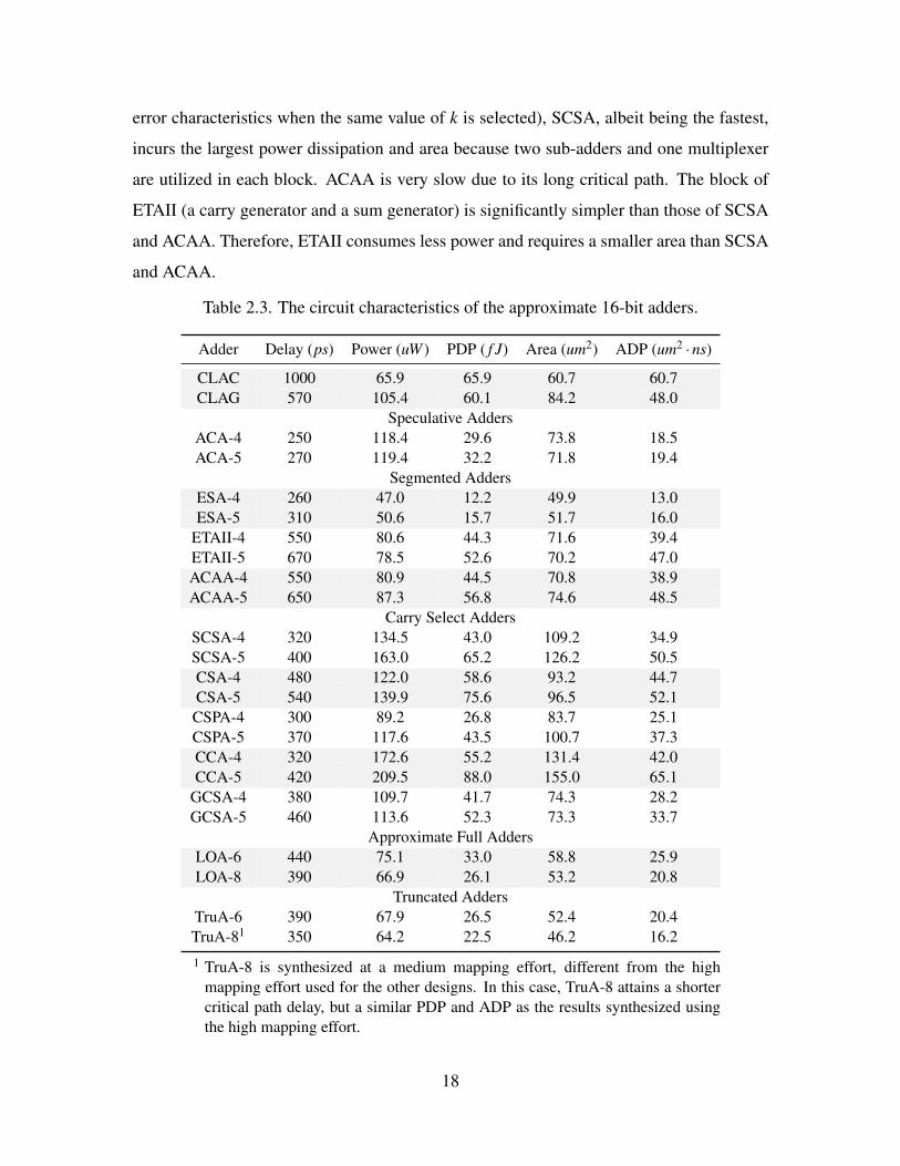
error characteristics when the same value of k is selected), SCSA, albeit being the fastest,

incurs the largest power dissipation and area because two sub-adders and one multiplexer

are utilized in each block. ACAA is very slow due to its long critical path. The block of

ETAII (a carry generator and a sum generator) is significantly simpler than those of SCSA

and ACAA. Therefore, ETAII consumes less power and requires a smaller area than SCSA

and ACAA.

Table 2.3. The circuit characteristics of the approximate 16-bit adders.

Adder Delay (ps) Power (uW ) PDP ( f J) Area (um2) ADP (um2 ·ns)

CLAC 1000 65.9 65.9 60.7 60.7CLAG 570 105.4 60.1 84.2 48.0

Speculative AddersACA-4 250 118.4 29.6 73.8 18.5ACA-5 270 119.4 32.2 71.8 19.4

Segmented AddersESA-4 260 47.0 12.2 49.9 13.0ESA-5 310 50.6 15.7 51.7 16.0

ETAII-4 550 80.6 44.3 71.6 39.4ETAII-5 670 78.5 52.6 70.2 47.0ACAA-4 550 80.9 44.5 70.8 38.9ACAA-5 650 87.3 56.8 74.6 48.5

Carry Select AddersSCSA-4 320 134.5 43.0 109.2 34.9SCSA-5 400 163.0 65.2 126.2 50.5CSA-4 480 122.0 58.6 93.2 44.7CSA-5 540 139.9 75.6 96.5 52.1CSPA-4 300 89.2 26.8 83.7 25.1CSPA-5 370 117.6 43.5 100.7 37.3CCA-4 320 172.6 55.2 131.4 42.0CCA-5 420 209.5 88.0 155.0 65.1

GCSA-4 380 109.7 41.7 74.3 28.2GCSA-5 460 113.6 52.3 73.3 33.7

Approximate Full AddersLOA-6 440 75.1 33.0 58.8 25.9LOA-8 390 66.9 26.1 53.2 20.8

Truncated AddersTruA-6 390 67.9 26.5 52.4 20.4TruA-81 350 64.2 22.5 46.2 16.2

1 TruA-8 is synthesized at a medium mapping effort, different from the highmapping effort used for the other designs. In this case, TruA-8 attains a shortercritical path delay, but a similar PDP and ADP as the results synthesized usingthe high mapping effort.

18

Fig. 2.10(b) shows that a circuit with a larger area is likely to consume more power.

Fig. 2.10 shows the delay, power, area, PDP and ADP of the equivalent adders. As

expected, the accurate CLAC has the longest delay among all adders, but not the highest

power dissipation. Compared to CLAC, CLAG is significantly faster and consumes more

power and area. TruA is not the fastest, but it is the most power and area-efficient design.

LOA is also more power and area efficient compared with most other approximate adders.

ESA is the slowest, but it is power and area efficient due to its simple segmentation

structure. CCA is the second fastest but is the most power and area consuming design due

to its complex speculative circuit. Both CSPA and GCSA have moderate power

dissipations, but CSPA is faster and GCSA uses a smaller area. Both the speed and power

dissipation of CSA are in the medium range. In terms of PDP and ADP, they show similar

trend. TruA, LOA and CSPA have very small values of PDP and ADP, while these values

are relatively large for CCA and CSA (shown in Fig. 2.10(c)).

0

200

400

600

800

1000

Del

ay (

ps)

(a) Delay

0.0

20.0

40.0

60.0

80.0

100.0

120.0

140.0

160.0

180.0Power (uW) Area (um²)

(b) Power and area

0.0

10.0

20.0

30.0

40.0

50.0

60.0

70.0PDP (fJ) ADP (um².ns)

(c) Power-delay product and area-delay product

Figure 2.10. A comparison of circuit measurements of the approximate adders.

As per Fig. 2.10, the carry select adders are likely to have large values of power

dissipation and area at a moderate performance. The segmented adders are power and

19

area-efficient. A speculative adder is relatively fast, but it is also more power hungry with

a moderate area. Conversely, the approximate full adder based adder is slow, but it

consumes a low power and area. The approximate full adders are more efficient in PDP

and ADP than most other approximate adders while the speculative adders are not. The

truncated adder is the most power and area efficient but with a relatively long delay.

Discussion

To compare the speed and power consumption, the approximate adders are further

synthesized using delay-optimization and area-optimization constraints, respectively. The

critical path delay of a design is constrained to the smallest value without timing violation

for a delay-optimization synthesis, whereas the area and power are optimized to the

smallest value for an area-optimization synthesis. Figs. 2.11 and 2.12 show the

comparison results of delay (delay-optimized) and power (area-optimized) considering

MRED and ER.

10-5 10-4 10-3 10-2 10-1

MRED

80

100

120

140

160

180

200

Del

ay (p

s)

ACAESAETAIIACAASCSACSACSPACCAGCSALOATruA

ESA

CSA

LOA

GCSA

ETAIIACAA

SCSA

TruA

ACA

CSPA

CCA

(a) MRED vs. Delay (delay-optimized)

10-1 100 101 102

ER (%)

80

100

120

140

160

180

200

Del

ay (p

s) ACAESAETAIIACAASCSACSACSPACCAGCSALOATruA

CSA

GCSA

ETAII

CCA TruALOA

ESA

ACAA

SCSA

CSPA

ACA

(b) ER vs. Delay (delay-optimized)

Figure 2.11. A comparison of delay for the approximate 16-bit adders.Note: The parameter k for LOA and TruA ranges from 3 to 9 from left to right, it is8 down to 3 for ESA and ACA, and it is from 6 down to 3 for the other adders fromleft to right.

CSA-6 is accurate due to the precise carry generated for every block, so the ER and

MRED of CSA-6 are 0; they are not shown in Figs. 2.11 and 2.12. Fig. 2.11 shows that,

among the adders with small MREDs, LOA and ETAII are faster than the other designs,

whereas CCA is the slowest followed by CSA. For a high MRED, ESA and CSPA are faster.

20

10-4 10-2 100

MRED

20

40

60

80

100

120

Pow

er (u

W)

ACAESAETAIIACAASCSACSACSPACCAGCSALOATruA

ESA

ETAII

ACAA

SCSA

CSPA

ACACCA

GCSA

LOA

TruA

CSA

(a) MRED vs. Power (area-optimized)

10-1 100 101 102

ER (%)

20

40

60

80

100

120

Pow

er (u

W)

ACAESAETAIIACAASCSACSACSPACCAGCSALOATruA

ETAIIGCSA

ACAA

SCSA

ACA

CCA

CSPALOA

ESA

TruA

CSA

(b) ER vs. Power (area-optimized)

Figure 2.12. A comparison of power for the approximate 16-bit adders.

When the same ER is considered, ETAII, SCSA and ACAA are among the fast designs. In

terms of power consumption, LOA and TruA are the most efficient, while ACA and CCA

are relatively power hungry, when a similar MRED is required, as shown in Fig. 2.12.

However, LOA and TruA have significantly high ERs. CSA has a rather low ER; ETAII

and ACAA are power-efficient, while ACA and CCA consume relatively high power for a

similar ER.

Since the ADP shows a similar trend as the PDP, the PDP (without delay or area

optimization) is considered for a comprehensive comparison of the approximate adders, as

shown in the two-dimensional (2-D) plots of Fig. 2.13. The equivalent adders are marked

by circles. Among adders with the same accuracy (ETAII, SCSA and ACAA), ETAII is

the most efficient in terms of delay, power and area. Thus, it is shown as a representative

in Fig. 2.13. Compared with the other approximate adders, CCA has the largest PDP and

moderate ER and MRED. Among the schemes with moderate PDPs (CSPA, GCSA and

ETAII), ETAII and GCSA have moderate MREDs and ERs, while CSPA shows slightly

higher values of these measures. ESA has a rather small PDP but a considerably large ER

and MRED. ACA has a larger PDP than ESA, but it has both lower ER and MRED. CSA

has a very high accuracy and a moderate PDP.

With the highest ERs, LOA and TruA show the smallest PDPs for a similar MRED due

to their low power dissipation. In fact, these approximate adders show a decent tradeoff

21

10 20 30 40 50 60 70 80 90 100PDP (fJ)

10-2

10-1

100

101

102

ER (%

)

ACAESAETAIIGCSACSACSPACCALOATruA

ETAIIACA

TruALOAESA

CSPA

CCA

CSA

GCSA

(a) ER vs. PDP

0 10 20 30 40 50 60 70 80 90 100PDP (fJ)

10-2

10-1

100

101

102

MR

ED (1

0-3)

ACAESAETAIIGCSACSACSPACCALOATruA

CCA

TruA

LOAGCSA

CSPA

ACA

ETAII

ESA

CSA

(b) MRED vs. PDP

Figure 2.13. A comprehensive comparison of the approximate 16-bit adders.Note: The parameter k for LOA and TruA ranges from 9 down to 3 from left to right, it is 3to 8 for ESA and ACA, and it is from 3 to 6 for the other adders from left to right. The addersmarked by circles are equivalent in terms of carry propagation and are thus representativesof different designs.

between error distance and hardware efficiency. In particular, they are useful in applications

in which hardware efficiency is of the utmost importance.

Table 2.4 shows the summary of different approximate adders, where their advantages

and disadvantages are highlighted (i.e., the metrics with moderate values are not shown).

As the MRED and NMED of approximate adders show similar trends, they are represented

by the error distance (ED) in the table.

22

Table 2.4. Summary of approximate adders.

AdderAccuracy Circuit

ER ED Average error speed power PDPACA high highESA high high high low low

ETAIIACAASCSACSA low low lowCSPA high high highCCA low high high

GCSALOA high low low high low lowTruA high high low low

2.3 Approximate Multipliers

2.3.1 Classification

Generally, a multiplier consists of stages of partial product generation, accumulation and

a final addition, as shown in Fig. 2.14 for a 4× 4 unsigned multiplication. Let Ai and

B j be the ith and jth least significant bits of inputs A and B respectively, a partial product

Pj,i is usually generated by an AND gate (i.e., Pj,i = AiB j). The commonly used partial

product accumulation structures include the Wallace, Dadda trees and a carry-save adder

array [126]. The Wallace tree for a 4×4 unsigned multiplier is shown in the dotted box of

Fig. 2.14. The adders in each layer operate in parallel without carry propagation, and the

same operation repeats until two rows of partial products are left. For an n-bit multiplier,

log(n) layers are required in a Wallace tree. Therefore, the delay of the partial product

accumulation stage is O(log(n)). Moreover, each adder in Fig. 2.14 can be considered

to be a (3:2) compressor and could be replaced by other counters or compressors (e.g., a

(4:2) compressor) to further reduce the delay. The Dadda tree has a similar structure as the

Wallace tree, but it uses as few adders as possible.

A carry-save adder array is shown in Fig. 2.15; the carry and sum signals generated

by the adders in a row are passed on to the adders in the next row. Adders in a column

operate in series. Hence the partial product accumulation delay of an n-bit multiplier is

23

A

B

Multiplicand

Multiplier

Partial products

×

Products

Wallace tree

Partial products generation

Partial products reduction

Final addition

Figure 2.14. The basic arithmetic process of a 4×4 unsigned multiplication with possibletruncations to a limited width.Note: : an input, a partial product or an output product; : a truncated bit; : a full adder or a half adder.

FAFAFA

FAFA

FA

FA

FAFA

P0,0P0,1P0,2P0,3

P1,0P1,1P1,2P1,3

P2,0P2,1P2,2P2,3

P3,0P3,1P3,2P3,3

FA

C0,0C0,1C0,2 S0,1S0,2

C2,0C2,1C2,2 S21S2,2

S0,0

S2,0

C3,0C3,1C3,2 S3,1S3,2 S3,0

HA

HA

HA

HAHAHA HA

C0,3 S0,3

C1,0C1,1C1,2 S1,1S1,2 S1,0C1,3 S1,3

C2,3 S2,3

C3,3 S3,3

‘0’‘0’‘0’‘0’

Figure 2.15. Partial product accumulation of a 4×4 unsigned multiplier using a carry-saveadder array.

approximately O(n) longer than that of the Wallace tree. However, such an array requires

a smaller area due to the simple and symmetric structure.

Three main methodologies are used for the approximate design of a multiplier: i)

approximation in generating the partial products [77], ii) approximation (including

truncation) in the partial product tree [9, 78, 101], and iii) using approximate designs of

adders [90], counters [87] or compressors [99,117] to accumulate the partial products. For

a signed integer operation, Booth multipliers have been widely used due to the fast

operation on a reduced number of partial products. Some recent designs use shifting and

addition to obtain the final product by rounding the inputs to a form of 2m (m is a positive

integer) [53, 113, 156].

24

Based on the different schemes in approximation, approximate multipliers are

classified into three unsigned types and signed Booth multipliers. Following this

classification, published designs of approximate multipliers are briefly reviewed next.

Approximation in generating partial products

The underdesigned multiplier (UDM) utilizes an approximate 2×2 multiplier obtained by

altering a single entry in the Karnaugh Map (K-Map) of its function (as highlighted in

Table 2.5) [77]. Table 2.5 shows the K-Map of the approximate 2× 2 multiplier, where

A1A0 and B1B0 are the two 2-bit inputs, and M2M1M0 is the 3-bit output. In this

approximation, the accurate multiplication result "1001" is simplified to "111" to save one

output bit when both the inputs are "11." Assuming the value of each input bit is equally

likely to take either "0" or "1," the error rate of the 2× 2 multiplier is then (12)

4 = 116 .

Larger multipliers can be designed based on the 2 × 2 multiplier. This multiplier

introduces an error when generating the partial products, however the adder tree for the

partial product accumulation remains accurate.

Table 2.5. K-Map for the 2×2 underdesigned multiplier block.

M2M1M0B1B0

00 01 11 10

A1A0

00 000 000 000 000

01 000 001 011 010

11 000 011 111 110

10 000 010 110 100

Approximation in the partial product tree

A bio-inspired imprecise multiplier, referred to as a broken-array multiplier (BAM), is

proposed in [101]. The BAM operates by omitting some carry-save adders in an array

multiplier in both the horizontal and vertical directions (Fig. 2.16). A more

straightforward approach to truncation is to truncate some LSBs on the input operands so

25

that a smaller multiplier is sufficient for the remaining most significant bits (MSBs). This

truncated multiplier (TruM) is considered as a baseline design.

Vertical Break Level (VBL)

Horizontal Break Level (VBL)

Horizontally-omitted cell Vertically-omitted cell

Figure 2.16. The broken-array multiplier (BAM) with 4 vertical lines and 2 horizontal linesomitted. : a carry-save adder cell.

The error tolerant multiplier (ETM) is divided into a multiplication section for the

MSBs and a non-multiplication section for the LSBs [78]. Fig. 2.17 shows the architecture

of a 16-bit ETM. A NOR gate-based control block is used to deal with the following two

cases: i) if the product of the MSBs is zero, then the upper accurate 8-bit multiplier is

activated to multiply the LSBs without any approximation, and ii) if the product of the

MSBs is nonzero, the non-multiplication section is used as an approximate multiplier to

process the LSBs, while the multiplication section is activated to accurately multiply the

MSBs.

Standard 8-bit Multiplier

LSB Non-multiplication block

Standard 8-bit Multiplier

A0-A7 B0-B7

P0-P15

A0-A7 B0-B7

A8-A15 B8-B15

P0-P15

P16-P31

Control Block

A8-A15 :

B8-B15 :

Figure 2.17. The 16-bit error-tolerant multiplier (ETM) of [78].

The static segment multiplier (SSM) was proposed using a similar partition scheme

[123]. Different from ETM, no approximation is applied to the LSBs in the SSM. Either

26

the MSBs or the LSBs of the operands are accurately multiplied depending on whether its

MSBs are all zeros. [64] showed that only small improvements in accuracy and hardware

are achieved compared to ETM, thus this design is not further considered in this comparison

study.

A power and area-efficient approximate Wallace tree multiplier (AWTM) is based on a

bit-width aware approximate multiplication and a carry-in prediction method [9]. An n×n

AWTM is implemented by four n/2× n/2 sub-multipliers, as shown in Fig. 2.18, where

the most significant sub-multiplier AHBH is further implemented by four n/4 × n/4

sub-multipliers. The AWTM is configured into four different modes by the number of

approximate n/4× n/4 sub-multipliers in the most significant n/2× n/2 sub-multiplier,

while the other three multipliers (AHBL, ALBH and ALBL) are approximate. The

approximate partial products are then accumulated by a Wallace tree.

AL BL

AL BH

AH BL

Final Product (2n bits)

n bits

n/2 bits

AHH BHH AHL BHL

AHL BHH

AHH BHL

AH BH

n/4 bits

Figure 2.18. The basic structure of the approximate Wallace tree multiplier (AWTM).Note: n is the width of the multiplier, AHBH , ALBH , AHBL and ALBL are partial products generated bythe n/2×n/2 sub-multipliers, AHHBHH , AHLBHH , AHHBHL and AHLBHL are partial products generatedby the n/4×n/4 sub-multipliers.

Using approximate counters or compressors in the partial product tree

An approximate (4:2) counter is proposed in [87] for an inaccurate 4-bit Wallace

multiplier. Table 2.6 shows the K-Map of the approximate (4:2) counter, where X1 · · ·X4

are the four input signals of a (4:2) counter (i.e., the partial products in the partial product

tree of a multiplier), C and S are the carry and sum, respectively. The values of CS in the

box are approximated as "10" for "100" in the approximate counter when all input signals27

are "1." As the probability of obtaining a partial product of "1" is 14 , the error rate of the

approximate (4:2) counter is (14)

4 = 1256 . The inaccurate 4-bit multiplier is then used to

construct larger multipliers with error detection and correction circuits. This approximate

multiplier is referred to as ICM. Approximate counters, in which the more significant

output bits are ignored, are presented and evaluated in [72]. Several signed multipliers are

then implemented using these approximate counters.

Table 2.6. K-Map for the 4 : 2 approximate counter.

CSX1X0

00 01 11 10

X3X4

00 00 01 10 01

01 01 10 11 10

11 10 11 10 11

10 01 10 11 10

In the compressor-based multiplier, accurate (3:2) and (4:2) compressors are improved

to speed up the partial product accumulation [7]. By using the improved compressors,

better energy and delay characteristics are obtained for a multiplier. To further reduce

delay and power, two approximate (4:2) compressor designs (AC1 and AC2) are presented

in [117]; these compressors are used in a Dadda multiplier with four different schemes.

The more accurate schemes 3 and 4 of the approximate compressor based multiplier

whose lower half partial products is accumulated by approximate compressors (referred to

as ACM-3 and ACM-4) in [117] are considered for comparison.

In the approximate multiplier with configurable error recovery, the partial products are

accumulated by a novel approximate adder (Fig. 2.19) [90]. The approximate adder utilizes

two adjacent inputs to generate a sum and an error bit. The adder processes data in parallel,

thus no carry propagation is required. Two approximate error accumulation schemes are

then proposed to alleviate the error of the approximate multiplier (due to the approximate

adder). OR gates are used in the first error accumulation stage in scheme 1 (AM1), while

in scheme 2 (AM2), both OR gates and the approximate adders are used. The truncation of

28

half of the LSBs in the partial products in AM1 and AM2 results in truncated approximate

multipliers TAM1 and TAM2, respectively [89].

Figure 2.19. The approximate adder cell. Si: the sum bit; Ei: the error bit.

Approximate Booth multipliers

The Booth recoding algorithm handles binary numbers in 2’s complement. The modified

(or radix-4) Booth algorithm is commonly used due to its ease in generating partial

products. Little work has been reported for approximate Booth multipliers, whereas the

fixed-width Booth multiplier that utilizes a truncation-based approach has been studied for

more than a decade. The conventional post-truncated fixed-width multiplier generates an

output with the same width as the input operand by truncating the lower half of the

product. Truncation of half of the partial products is widely used because the

post-truncated scheme does not achieve a significant circuit advantage over the accurate

multiplier. The direct truncation of partial products incurs a large error, so many error

compensation schemes have been proposed [24, 28, 111, 145]. Another approach is to use

an approximate Booth encoder with a simple circuit [94]. Most of the approximate Booth

multipliers are based on the modified Booth algorithm; the partial products are

accumulated by an array structure in [28, 40, 111, 145] while a parallel carry-save-adder

tree is used in [24, 94].

Fig. 2.20 shows the partial products of an 8×8 fixed-width modified Booth multiplier

with error compensation [28]. The final product is the addition of the main part (MP) and

the carry signals generated in the truncation part (TP). The carry signals are approximated

by the output of Booth encoders. The approximate carry σ is σ =

⌊2−1(

n/2−2∑

i=0zeroi +1)

⌋,

where n is the multiplier width, and zeroi is "1" if the ith partial product vector is not zero

or zeroi = 0 otherwise. This multiplier is referred to as BM04.

29

P0,0P0,2P0,4P0,6 P0,1P0,3P0,5P0,7P0,8

P1,0P1,2P1,4P1,6 P1,1P1,3P1,5P1,7P1,8

P2,0P2,2P2,4P2,6 P2,1P2,3P2,5P2,7P2,8

P3,0P3,2P3,4P3,6 P3,1P3,3P3,5P3,7P3,8

Main Part (MP) Truncation Part (TP)

n0

n1

n2

n3 TPmajor

TPminor

exact carry approximate carry

Figure 2.20. The partial products for an 8×8 fixed-width modified Booth multiplier [28].Note: Pi, j is the jth partial product in the ith partial product vector and ni is the sign of the ith partial productvector.

The multiplier in [111] can adaptively compensate the quantization error by keeping

different numbers of the most significant columns of the partial products (ω (ω ≥ 0)). Two

types of binary thresholding are proposed for error compensation. Different from BM04,

n rather than (n−1) columns of partial products are truncated for an n×n multiplier. The

error compensation for each type of binary thresholding varies with the value of ω and the

partial products of the ω th column in the truncation part (from left to right). This multiplier

is denoted by BM07.

The multiplier presented in [145] uses n columns of partial products in the truncation

part for an n× n multiplier; the most significant one column in the truncation part is

reserved for error compensation. The error compensation using a simplified sorting

network significantly reduces the mean and mean-squared errors by making the error

symmetric as well as centralizing the error distribution around zero. This design is

referred to as BM11.

A fixed-width Booth multiplier was designed based on a probabilistic estimation bias

in [24]. Therefore, this multiplier is referred to as PEBM. The number of columns of

the accumulated partial products varies in accordance with the desired trade-off between

hardware and accuracy. The error compensation formula is derived from a probability

analysis rather than a time-consuming exhaustive simulation. The carry generated by the

truncation part is approximated by σ =

⌊2−1(

n/2−1−bω/2c∑

i=0zi−1)

⌋, where zi = P0,n/2−1 +

nn/2−1 when i is n/2−1 and zi = zeroi otherwise.

Based on the BAM, the broken Booth multiplier (BBM) uses a modified Booth

algorithm to generate partial products and omits full adders to the right of a vertical line

30

[40]. BBM has a smaller PDP for the same mean-squared error compared to BAM.

Similar to the unsigned multiplier, the truncated radix-4 Booth multiplier (TBM) is

considered as a baseline design for the signed multiplier. TBM-k is obtained by truncating

the k LSBs of the input operands in a modified Booth multiplier.

In [94], two approximate Radix-4 Booth encoders are designed for the partial product

generation by simplifying the exact K-Map. The generated partial products are then

accumulated using exact 4-2 compressors.

2.3.2 EvaluationError Characteristics

The considered 16×16 approximate multipliers are simulated in MATLAB with 10 million

uniformly distributed random input combinations. The ER, NMED, MRED and average

error are obtained and shown in Table 2.7. TruM-k represents the truncated multiplier with

k LSBs truncated in the input operands.

According to Table 2.7, most of the designs, especially those with truncation, have

significantly large ERs close to 100%. However, ICM has a relatively low ER of 5.45%,

because it uses just one approximate counter in a 4× 4 sub-multiplier with an error rate

of only 1256 . UDM also shows a lower ER than the other approximate multipliers. In

terms of the average error, ACMs have the smallest value, while the average errors for all

the other approximate unsigned multipliers show the same trend with the NMED. This

is because ACMs produce both positive and negative errors, but the other approximate

unsigned multipliers produce either negative or positive errors.

Fig. 2.21 shows the NMEDs and MREDs of the equivalent approximate multipliers that

are configured to have 16-bit accurate MSBs (except for ICM and UDM that have only one

configuration). Thus, the truncated LSBs in the partial product is 16 for BAM, the number

of MSBs used for error compensation is 16 for AM1, AM2, TAM1 and TAM2, the size

of the accurate sub-multiplier is 8 for ETM, 8 LSBs are truncated for TruM, and the mode

number of ACM and AWTM is 4. Among the unsigned approximate multipliers, UDM

has the largest NMED while ACM has the smallest. ICM, AM2 and TAM2 have similar

values of NMED; however, ICM has the smallest MRED, while the MRED of TAM2 is

the largest. Therefore ICM has the highest accuracy in terms of MRED, while TAM2 is the

31

Table 2.7. The error characteristics of the approximate 16×16 multipliers

Multiplier ER (%) NMED (10−3) MRED (%) Average Error (10−3)

Multipliers with Approximation in Generating Partial ProductsUDM 80.99 13.92 3.33 -13.9

Multipliers with Approximation in the Partial Product TreeBAM-16 99.99 0.06 0.21 -0.06ETM-8 100.00 1.94 2.85 -1.9

AWTM-4 99.94 0.02 0.33 0.02Multipliers using Approximate Counters or Compressors

ICM 5.45 0.29 0.06 -0.3ACM-4 99.97 0.01 0.26 0.003AM1-16 98.22 0.81 0.34 -0.8AM2-16 97.96 0.27 0.13 -0.3

TAM1-16 99.99 1.06 0.58 -1.1TAM2-16 97.99 0.28 0.22 -0.3

Truncated Unsigned MultipliersTruM-4 99.61 0.11 0.23 -0.1TruM-8 100.0 1.94 2.85 -1.94

Approximate Booth MultipliersPEBM 99.99 0.023 0.27 -0.01BBM 100.00 0.092 0.57 -0.09BM11 99.99 0.022 0.18 −7.0×10−6

BM07 99.99 0.024 0.16 -0.01BM04 99.99 0.027 0.48 -0.02TBM-4 99.61 0.172 0.47 1.3×10−4

Note: The parameter k follows the acronym of each approximate multiplier. For AM1,AM2, TAM1 and TAM2, this parameter refers to the number of MSBs used for errorreduction and for ETM, the number of LSBs in the inaccurate part. It is the mode numberin AWTM and ACM, and the vertical broken length for BAM. In TruM and TBM, theparameter is the number of truncated LSBs in the input operands.

least accurate among these three approximate multipliers. This indicates that multipliers

with simple truncation tend to have larger MREDs when their NMEDs are similar. BAM

has moderate values of NMED and MRED, while ETM and TruM have both large MRED

and NMED.

Hence, ICM is the most accurate design with the lowest ER, MRED and a moderate

NMED. ACM, AWTM, BAM, AM2 and TAM2 also show good accuracy among all the

considered approximate multipliers with both low NMEDs and MREDs. ETM, TruM and

UDM are relatively inaccurate in terms of these metrics.

32

-3.0

-2.0

-1.0

0.0

1.0

2.0

ER (log) average error (10-3)

-14.0

(10-3)~~

(a) ER and average error

0.0001

0.001

0.01

0.1

1

10

MRED (%) NMED (%)

(b) NMED and MRED

Figure 2.21. A comparison of error characteristics of the approximate 16×16 multipliers.Note: ACM and AWTM represent ACM-4 and AWTM-4, respectively. The truncated number of LSBs inthe partial product is 16 for BAM, the number of MSBs used for error compensation is 16 for AM1, AM2,TAM1 and TAM2, and 8 LSBs are truncated for TruM. ETM is ETM-8.

For the approximate Booth multipliers in Table 2.7, a column of the most significant

partial products in the truncation part (adjacent to the MP part) is kept for PEBM, BM07

and BM04. 15-bit columns of partial products are truncated in BBM to keep the same width

of the output as the other designs. The ERs of all approximate Booth multipliers are close

to 100% due to truncation. Most designs have similar NMEDs except for BBM and TBM.

BBM has the largest NMED and MRED because there is no error compensation. TBM-4

has a similar MRED as BBM; however, it shows a larger NMED and smaller average error

than the other approximate Booth multipliers. BM07 and BM11 have very small MRED

values, while PEBM has a slightly larger value. BM11 has the smallest average error.

In summary, as a multiplier approximated in generating the partial products, UDM has

relatively large values of NMED and MRED, and a relatively small ER. The multipliers

approximated in the partial product tree mostly have moderate NMEDs and relatively large

MREDs (except for BAMs with fewer than or equal to 18 truncated bits and AWTM-

4). The multipliers approximated using approximate counters or compressors have small

values of both NMED and MRED, while the multiplier truncated on the input operands

have large values of both metrics (when the truncated number of LSBs is larger than 4).

Among the considered approximate Booth multipliers, BBM and TBM-4 show the lowest

accuracy in terms of both NMED and MRED. BM11 has the smallest average error. The

other approximate Booth multipliers show similar NMEDs and various MREDs.

33

Circuit Characteristics

The 16×16 approximate multipliers are implemented in VHDL and synthesized using the

same tool and process as in the simulation of approximate adders. The only difference

is that the clock period is 4 ns for the power estimation of the multipliers because of a

longer critical path delay. The accurate Wallace multiplier (WallaceM) optimized for speed

[124] and the array multiplier (ArrayM) are also simulated for comparison. To reduce the

effect of the final addition, the same multi-bit adder in the tool library is utilized in all

approximate multiplier designs as the final adder. Table 2.8 shows the critical path delay,

area, power, PDP and ADP of the considered multipliers. TruMA and TruMW denote the

truncated array and Wallace multipliers, respectively.

Table 2.8. Circuit characteristics of the approximate multipliers

Multiplier Delay (ns) Power (uW ) PDP ( f J) Area (um2) ADP (um2 ·ns)

ArrayM 2.58 477.4 1,231.7 921 2,375.7WallaceM 2.03 461.3 936.4 934 1,896.0

Multipliers with Approximation in Generating Partial ProductsUDM 2.01 352.7 708.9 829 1666.7

Multipliers with Approximation in the Partial Product TreeBAM-16 2.34 221.3 517.8 441 1,031.9ETM-8 1.50 108.5 162.8 288 431.4

AWTM-4 1.74 280.0 478.2 715 1,243.2Multipliers using Approximate Counters or Compressors

ICM 1.87 367.4 687.0 937 1,751.4ACM-4 2.00 284.1 568.2 724 1,447.0AM1-16 1.57 380.6 597.5 878 1,378.5AM2-16 1.71 400.4 684.7 1,051 1,797.2

TAM1-16 1.45 214.6 311.2 516 748.2TAM2-16 1.62 244.9 396.7 693 1,122.7

Truncated Unsigned MultipliersTruMA-4 1.89 243.5 460.2 503 950.6TruMA-8 1.19 92.1 109.6 211 250.5TruMW-4 1.62 262.4 425.1 561 908.2TruMW-8 1.10 98.4 108.2 239 263.0

Approximate Booth MultipliersPEBM 1.83 264.3 483.7 528 966.2BBM 1.91 250.3 478.1 487 930.2BM11 1.96 258.1 505.9 475 931.0BM07 2.03 270.4 548.9 528 1071.8BM04 2.05 249.8 512.1 447 916.4TBM-4 1.88 272.8 512.8 517 972.3

34

Fig. 2.22 shows the comparison of delay, power , area, PDP and ADP of the equivalent

approximate multipliers. The accurate array multiplier (ArrayM) is the slowest design and

the Wallace multiplier (WallaceM) consumes a relatively large area (as per Table 2.8); this

is consistent with the theoretical analysis. Due to the expressively fast carry-ignored

operation, AM1/TAM1, AM2/TAM2 have smaller delays compared to most of the other

designs. BAM is significantly slower due to its array structure. AWTM, UDM, ICM and

ACM have larger delays than the other approximate multipliers. BAM consumes a

relatively low power, the power consumptions of AWTM and ACM are in the medium

range, while UDM and ICM incur a relatively high power consumption. TruMA, TruMW

and ETM have both a short delay and a low power dissipation.

0.0

0.5

1.0

1.5

2.0

2.5

Del

ay (

ns)

(a) Delay

0.0

200.0

400.0

600.0

800.0

1000.0Power (uW) Area (um²)

(b) Power and area

0

500

1000

1500

2000

2500PDP (fJ) ADP (um².ns)

(c) Power-delay product and area-delay product

Figure 2.22. A comparison of circuit measurements of the approximate 16×16 multipliers.

A multiplier with a higher power dissipation usually has a larger area and thus a larger

PDP and ADP. In terms of power and area, TruMA, TruMW, ETM, TAM1/TAM2 and

BAM are among the best designs. A common feature of these designs is that they all

use truncation, which can significantly affect the MRED while the NMED may not be35

significantly changed. If most of the inputs have large values, the error introduced by

truncation can be tolerated; thus truncation is a useful scheme to save area and power.

Otherwise, truncation-based designs may yield unacceptably inaccurate results. Without

truncation, a multiplier whose design is approximated in generating partial product (e.g.

UDM) tends to have a large delay, power and area. These measures for the multipliers that

approximate in the partial product tree (e.g. AWTM) are moderate, while the multipliers

using approximate counters or compressors (ICM, ACM, AM1, AM2) require higher power

and area.

In terms of PDP and ADP (Fig. 2.22(c)), TruMA, TruMW, ETM, TAM1 and TAM2

have very small values, while ICM, UDM and AM2 are the opposite. The values of PDP

and ADP for AM1, ACM, BAM and AWTM are in the medium range.

For the approximate Booth multipliers, PEBM is the fastest, but it is relatively high in

power and area consumption due to the use of a carry save adder tree for the parallel

accumulation. With no error compensation, BBM shows a small delay, low power

dissipation and small circuit area, and thus smaller PDP and ADP compared with most of

the other designs (BM04). BM11 and BM04 have similar values for all circuit metrics.

BM07 has a similar delay, but with a higher power and area and thus a larger PDP and

ADP, compared with BM04.

Discussion

Figs. 2.23 and 2.24 show the speed and power dissipation of approximate unsigned

multipliers considering MRED and NMED. Fig. 2.23 shows that ICM and TruMW are

faster than the other designs for a small MRED and NMED, whereas TAM1 is the fastest

when the MRED and NMED are larger. AM1, AM2 and TAM2 are also fast; BAM, ETM

and TruMA show relatively low speed. As shown in Fig. 2.24, BAM is the most

power-efficient followed by TruMA, while UDM and ACM are relatively power hungry.

The power dissipations of TAM1 and TAM2 are in the medium range. AWTM (except for

AWTM-4) has a larger MRED and a higher power consumption than the other designs.

The speed and power dissipation comparison of approximate Booth multipliers are

shown in Figs. 2.25 and 2.26, respectively. Among the considered designs, PEBM is the

fastest and relatively power-efficient; BM07 is the slowest with a relatively high power

36

10-3 10-2 10-1 100 101 102

MRED (%)

0.4

0.5

0.6

0.7

0.8

0.9

1

Del

ay (n

s) UDMBAMETMAWTMICMACMAM1AM2TAM1TAM2TruMATruMW

TruMA

BAM

ETM

AWTM

UDM

AM2

TAM2

AM1

TAM1

TruMWACM

ICM

(a) MRED vs. Delay (delay-optimized)

10-4 10-2 100

NMED (%)

0.4

0.5

0.6

0.7

0.8

0.9

1

Del

ay (n

s) UDMBAMETMAWTMICMACMAM1AM2TAM1TAM2TruMATruMW

UDMTruMW

ACM TAM2ICM

AM2 AWTM

ETM

BAM

TruMA

AM1

TAM1

(b) NMED vs. Delay (delay-optimized)

Figure 2.23. A comparison of delay for the approximate 16×16 multipliers.Note: The number of truncated LSBs for TruMA and TruMW is from 2 to 8 from left toright; it is 11 to 22 for BAM. The number of MSBs used for error compensation is 16 downto 10 for AM1, AM2, TAM1 and TAM2. The size of the accurate sub-multiplier is from10 down to 8 for ETM. The mode number of AWTM is from 4 down to 1, and it is from 4down to 3 for ACM.

10-3 10-2 10-1 100 101 102

MRED (%)

100

150

200

250

300

350

Pow

er (u

W) UDM

BAMETMAWTMICMACMAM1AM2TAM1TAM2TruMATruMW

UDM

ICM

ACM

BAM

TruMAAM2

TruMW AM1 AWTM

ETM

TAM2

TAM1

(a) MRED vs. Power (area-optimized)

10-4 10-3 10-2 10-1 100 101

NMED (%)

100

150

200

250

300

350

Pow

er (u

W) UDM

BAMETMAWTMICMACMAM1AM2TAM1TAM2TruMATruMW

UDM

ETM

ACM

TAM1

BAM

ICM

TAM2TruMW

TruMA

AWTM

AM1AM2

(b) NMED vs. Power (area-optimized)

Figure 2.24. A comparison of power consumption for the approximate multipliers.

consumption. Compared to the other approximate Booth multipliers, TBM is much faster

but more power hungry, considering a similar MRED or NMED.

MRED and PDP (without delay or area optimization) are jointly considered next for

an overall evaluation of the approximate multipliers, as shown in Fig. 2.27 and Fig. 2.28.

Fig. 2.27 shows that TruMW has a smaller PDP than TruMA when the same number of

LSBs is truncated. Among the truncation-based designs, the truncated unsigned multipliers

37

0 0.5 1 1.5 2MRED (%)

0.54

0.56

0.58

0.6

0.62

0.64

0.66

Del

ay (n

s)

BM07BM11

BBM

PEBM

TBM

BM04

(a) MRED vs. Power (area-optimized)

10-3 10-2 10-1 100

NMED (%)

0.52

0.54

0.56

0.58

0.6

0.62

0.64

0.66

Del

ay (n

s)

BM07

BM11 BM04

BBM

TBM

PEBM

(b) NMED vs. Power (area-optimized)

Figure 2.25. A comparison of power consumption for the approximate Booth multipliers.Note: The number of truncated LSBs for TBM is from 2 to 6 from left to right.

10-1 100

MRED (%)

160

180

200

220

240

260

280

300

Pow

er (u

W)

BM07

BM04

BM11

BBM

PEBM

TBM

(a) MRED vs. Power (area-optimized)

10-2 10-1

NMED (%)

160

180

200

220

240

260

280

300

Pow

er (u

W)

TBM

BM04

BBMBM11PEBMBM07

(b) NMED vs. Power (area-optimized)

Figure 2.26. A comparison of power consumption for the approximate Booth multipliers.

(TruMA and TruMW) are slightly more accurate (in MRED) than BAM and ETM for a

similar PDP. TruMW has a smaller MRED than most other approximate designs (except

TAM1 and TAM2).

In Fig. 2.27, TAM1-13, TAM1-16, TAM2-13, TruMA-6, TruMW-6 and BAM-18 have

both small PDPs and MREDs. Most of the other designs have at least one major

shortcoming. ICM and ACM both incur a relatively low error, but their PDPs are

relatively high. Other than the truncated designs, ETM-8 has the smallest PDP but with a

rather large MRED. UDM shows a poor performance in both PDP and MRED. Even

38

100 200 300 400 500 600 700 800PDP (fJ)

10-1

100

MR

ED (%

)AM1-16

AM1-13

TAM1

AM2-16

AM2-13

AM2-10

TAM2

ETM-8

ETM-7

AWTM-4

AWTM-3

ICM

UDM BAM

ACM-3 ACM-4

TruMA

TruMW

Figure 2.27. MRED and PDP of the approximate unsigned multipliers.Note: The parameter k for TruMA and TruMW is from 8 down to 2 from left to right;it is 21 down to 13 for BAM, and 10 to 16 for TAM1 and TAM2. The multipliersmarked by circles are equivalent in terms of the number of accurate MSBs and arethus representatives of different designs.

350 400 450 500 550 600 650 700PDP (fJ)

10-1

100

MR

ED (%

)

TBM

BM04

BBM

PEBM

BM11BM07

Figure 2.28. MRED and PDP of the approximate Booth multipliers.Note: The parameter k for TBM is from 6 down to 2 from left to right.

though some BAM configurations have small PDPs, their delays are generally large

(Fig. 2.22(a)); moreover, some BAM configurations have low accuracies. AWTMs have

large PDPs and only AWTM-4 has a high accuracy.

39

Fig. 2.28 shows that most approximate Booth multipliers (except for BM04) consume

smaller PDPs than TBM considering a similar MRED. BM11 and BM07 are relatively

accurate in terms of MRED but with relatively poor PDPs. PEBM shows both a moderate

PDP and MRED.

A summary of the accuracy and circuit characteristics for approximate multiplier

designs is shown in Table 2.9. As almost all of the approximate multipliers have an ER of

close to 100%, except ICM and UDM, the ER is not considered in Table 2.9.

Table 2.9. Summary of the approximate multipliers.

MultiplierAccuracy Circuit

MRED NMED Average error speed power PDPUDM high high high high highBAM low low lowETM high low

AWTM high low highICM lowACM low low highAM1AM2

TAM1 high lowTAM2 lowTruMA high lowTruMW high high lowBM04BM07 low low high largeBM11 low low low lowPEBM low high low smallBBM high high high smallTBM high high low high high large

2.4 Approximate Dividers

2.4.1 Classification

The divider is a less frequently used arithmetic module compared to the adder and

multiplier; therefore, less research has been pursued on approximate designs.

Two methodologies have been advocated for sequential division: the digit recurrent

algorithm [93] and the functional iterative algorithm (e.g., using the Newton-Raphson

algorithm [42]). A sequential divider has a low hardware complexity, however its delay is

40

considerably longer than an adder and a multiplier, so it could significantly affect the

overall performance of a processor. Thus, dividers made of combinational logic circuits

are discussed in this chapter. Like multiplication, division can also be implemented by an

array structure, in which adder cells are replaced by subtractor cells, as shown in

Fig. 2.29. Several approximations are made on the array divider while retaining a

low-power [19, 20, 22] and high-speed [54] operation. In addition, different approximate

divider designs based on rounding [157] and curve fitting [97, 149] are also proposed.

q2 ‘0’

q1

r2 r1 r0

b3 b2 b1a7 a6 a5 a4

a1

a0

q3 ‘0’

q0

b0 a3

a2

‘0’

a1

‘0’

r3

Figure 2.29. An 8/4 unsigned restoring array divider with constituent subtractorcells [125].

Approximate array dividers

Four types of approximate unsigned non-restoring divider (AXDnr) are presented in [19].

Three approximate subtractors are designed for the array of an unsigned divider by

simplifying the circuit of an exact subtractor cell. The approximate subtractors are then

used to replace the exact subtractor cells at the least significant vertical, horizontal, square

or triangle cells of the array divider. Moreover, a truncation scheme is utilized by

discarding the approximate subtractors for comparison. Based on the same theory and

design, four types of approximate restoring divider using approximate subtractorss

(AXDrs) are further proposed [20]. It has been shown that AXDrs are slightly more

accurate and consume lower power than AXDnrs.

To make the remaining subtractor cells more efficient, a dynamic approximate divider

(DAXD) is proposed by dynamically selecting the inputs of the subtractor cells [54].

DAXD selects a fixed number of bits in the input operands from the most significant

41

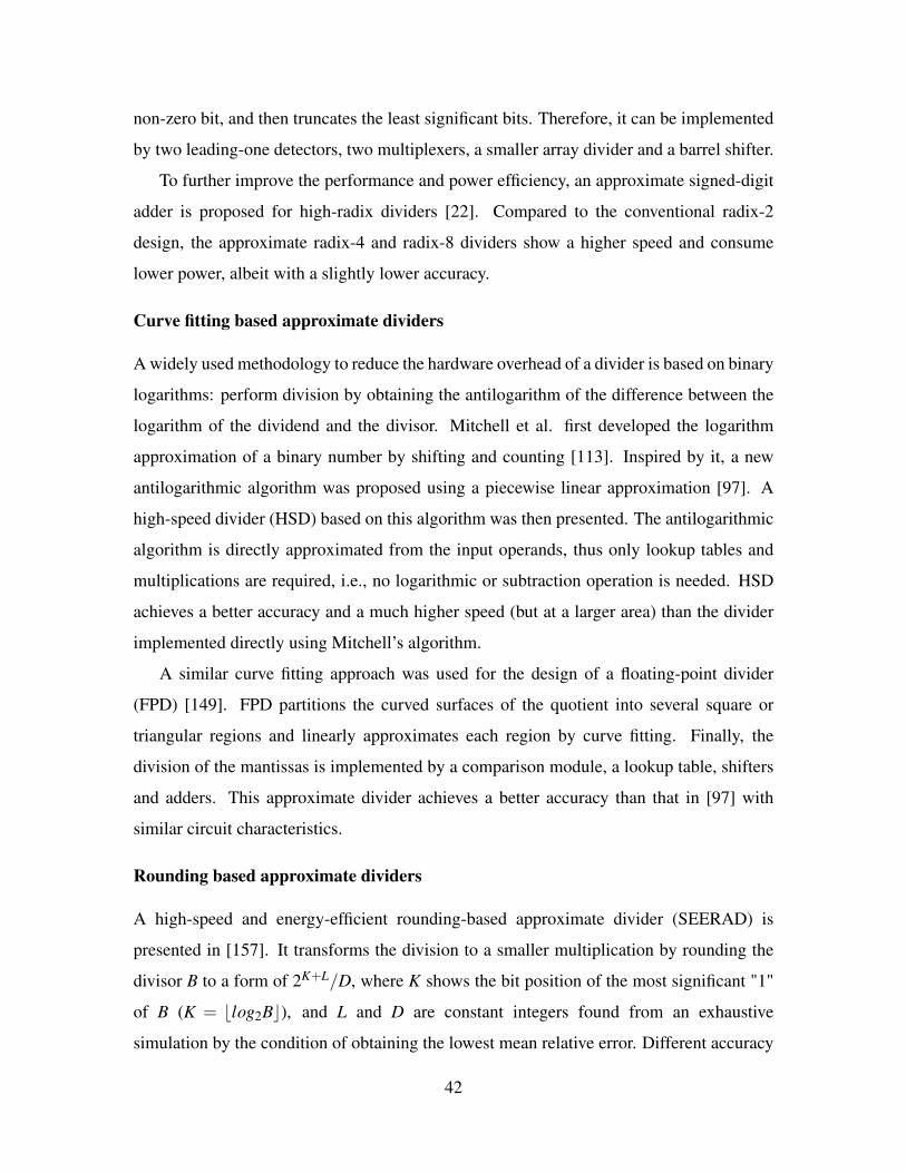
non-zero bit, and then truncates the least significant bits. Therefore, it can be implemented

by two leading-one detectors, two multiplexers, a smaller array divider and a barrel shifter.

To further improve the performance and power efficiency, an approximate signed-digit

adder is proposed for high-radix dividers [22]. Compared to the conventional radix-2

design, the approximate radix-4 and radix-8 dividers show a higher speed and consume

lower power, albeit with a slightly lower accuracy.

Curve fitting based approximate dividers

A widely used methodology to reduce the hardware overhead of a divider is based on binary

logarithms: perform division by obtaining the antilogarithm of the difference between the

logarithm of the dividend and the divisor. Mitchell et al. first developed the logarithm

approximation of a binary number by shifting and counting [113]. Inspired by it, a new

antilogarithmic algorithm was proposed using a piecewise linear approximation [97]. A

high-speed divider (HSD) based on this algorithm was then presented. The antilogarithmic

algorithm is directly approximated from the input operands, thus only lookup tables and

multiplications are required, i.e., no logarithmic or subtraction operation is needed. HSD

achieves a better accuracy and a much higher speed (but at a larger area) than the divider

implemented directly using Mitchell’s algorithm.

A similar curve fitting approach was used for the design of a floating-point divider

(FPD) [149]. FPD partitions the curved surfaces of the quotient into several square or

triangular regions and linearly approximates each region by curve fitting. Finally, the

division of the mantissas is implemented by a comparison module, a lookup table, shifters

and adders. This approximate divider achieves a better accuracy than that in [97] with

similar circuit characteristics.

Rounding based approximate dividers

A high-speed and energy-efficient rounding-based approximate divider (SEERAD) is

presented in [157]. It transforms the division to a smaller multiplication by rounding the

divisor B to a form of 2K+L/D, where K shows the bit position of the most significant "1"

of B (K = blog2Bc), and L and D are constant integers found from an exhaustive

simulation by the condition of obtaining the lowest mean relative error. Different accuracy

42

levels are considered to improve the accuracy of SEERAD by varying D and L with

combinations of the more relevant bits of B after the most significant "1." The multiplier

in SEERAD is implemented by several shift units and an adder block. Thus, SEERAD is

very fast.

2.4.2 EvaluationError Characteristics

As HSD and FPD are designed for floating-point division, AXDr, DAXD and SEERAD

are selected for the evaluation. Among the four types of AXDr, the triangle replacement

has been shown to achieve the best tradeoff [20]. Therefore, three designs of AXDr with

the triangle replacement, AXDr1 (using approximate subtractor 1), AXDr2 (using

approximate subtractor 2) and AXDr3 (using approximate subtractor 3), are evaluated. All

valid combinations in the range of [0,65535] and (0,255] are used as the input dividends

and divisors. They are carefully selected to meet the no overflow condition of an accurate

16/8 divider. The simulation results are shown in Table 2.10. The number following each

acronym is the parameter for each approximate design. It is the replacement depth and the

accuracy level for AXDrs and SEERAD, respectively. For DAXD, the parameter value is

the bit width of the selected dividend.

Among these designs, AXDr1 and AXDr3 have relatively small ERs, whereas

SEERAD has the largest ER that is close to 100%. DAXD and SEERAD of accuracy

levels 1 and 2 result in very large values of NMED. AXDr3 has significantly small

NMED and MRED yet with a relatively large average error. The MRED shows a similar

trend with the NMED except that AXDr2 with a depth of 10 results in a very large

MRED. The accuracy of DAXD is lower than the other designs due to the possible

overflow.

Circuit Measurements

To obtain the circuit measurements, the approximate dividers and the exact unsigned

restoring array divider (EXDr) are implemented in VHDL and synthesized using the same

process and tools as in the simulation of approximate adders. The clock period used for

power estimation is 5 ns, and the input combinations are 5 million random numbers. For

43

Table 2.10. Error characteristics of the approximate 16/8 dividers.

DividerER(%)

NMED(%)

MRED(%)

Average error(10−3)

AXDr1-10 80.94 1.32 4.32 -0.95AXDr1-9 71.12 0.67 2.45 -0.96

AXDr2-10 93.51 2.45 11.88 4.48AXDr2-9 88.19 1.33 6.20 0.99

AXDr3-10 78.64 0.97 3.25 11.89AXDr3-9 66.63 0.51 1.84 6.11

SEERAD-1 99.99 7.64 15.58 -13.75SEERAD-2 99.99 4.11 8.52 -12.97SEERAD-3 99.99 2.23 4.97 4.87SEERAD-4 99.99 1.09 2.71 -1.13DAXD-10 85.57 6.65 14.74 -62.00DAXD-12 75.77 6.39 13.41 -61.48

Note: The parameter follows the acronym of each approximatedivider. It is for the replacement depth and the accuracy level forAXDrs and SEERAD, respectively. For DAXD, the parameter is thebit width of the selected dividend.

ease of comparison, the same array structure and subtractor cells are used in the accurate

part of AXDrs and DAXD. The results are reported in Table 2.11.

Table 2.11. Circuit measurements of the considered dividers.

DividerDelay(ns)

Area(µm2)

Power(µW )

PDP( f J)

ADP(ns ·µm2)

EXDr 4.71 285.8 128.00 602.88 1,345.9AXDr1-10 4.38 280.2 113.90 498.88 1,227.3AXDr1-9 4.40 281.2 116.70 513.48 1,237.3AXDr2-10 4.65 252.6 94.68 440.26 1,174.7AXDr2-9 4.67 259.5 100.80 470.74 1,211.8AXDr3-10 4.38 216.6 59.98 262.71 948.6AXDr3-9 4.39 227.3 70.38 308.97 998.0SEERAD-1 1.15 204.3 56.04 64.45 235.0SEERAD-2 2.02 253.1 80.61 162.83 511.3SEERAD-3 1.81 333.4 107.80 195.12 603.5SEERAD-4 2.23 480.1 169.80 378.65 1,070.7DAXD-10 2.73 245.5 63.83 174.26 670.1DAXD-12 3.69 286.9 86.99 320.99 1,058.7

Among all considered designs, SEERAD shows the shortest delay because its critical

path is significantly reduced due to the use of a multiplier instead of a divider structure.

44

However, SEERAD incurs a large area and high power consumption when its accuracy level

is 3 or 4 due to the lookup table used for storing the constants. Although SEERAD-1 (for

accuracy level 1) and SEERAD-2 (for accuracy level 2) are more power and area-efficient

with a very short delay, their accuracy is significantly lower than the other approximate

dividers, as shown in Table 2.10.

The hardware improvements for AXDr1 and AXDr2 are very minor compared with

the accurate counterpart, although the power and area reductions are larger for AXDr3.

Moreover, AXDrs are the slowest because replacing the exact subtractors with approximate

ones does not significantly reduce the carry/borrow chain on the critical path. DAXD shows

a rather small delay and power dissipation, but its area is slightly larger than the accurate

design when a 12/6 accurate divider is used.

Discussion

The critical path delay (delay-optimized) and power consumption (area-optimized) of the

approximate dividers are compared in Figs. 2.30 and 2.31, respectively. For a small MRED

or NMED, AXDr1 is the fastest, and AXDr3 is the most power-efficient. The SEERAD

has a higher speed considering a larger MRED or NMED.

100 101

MRED (%)

100

Del

ay (n

s)

AXDr1

AXDr3AXDr2

DAXD

SEERAD

(a) MRED vs. Delay (delay-optimized)

100

NMED (%)

100

Del

ay (n

s)

AXDr1

AXDr3AXDr2

DAXD

SEERAD

(b) NMED vs. Delay (delay-optimized)

Figure 2.30. A comparison of power consumption for the approximate dividers.Note: The replacement depths of AXDr1, AXDr2 and AXDr3 are from 8 to 11 from left to right.The accuracy levels of SEERAD are from 4 down to 1 from left to right. The pruned dividendwidth is from 12 down to 8 for DAXD from left to right.

45

100 101

MRED (%)

50

100

150

200

Pow

er (u

W)

SEERAD

AXDr3

AXDr1

AXDr2

DAXD

(a) MRED vs. Power (area-optimized)

100

NMED (%)

50

100

150

200

Pow

er (u

W)

AXDr1

AXDr3

AXDr2

SEERAD

DAXD

(b) NMED vs. Power (area-optimized)

Figure 2.31. A comparison of power consumption for the approximate dividers.

A qualitative comparison for different approximate dividers in terms of different metrics

is shown in Table 2.12. Also, their PDPs and MREDs are jointly compared, as shown in

Fig. 2.32. This figure illustrates that AXDr3 is a good design for applications requiring

high-accuracy. Although some configurations of AXDr1 and AXDr2 show small MREDs,

their PDPs are generally large. On the contrary, DAXD has a relatively small PDP but a

significantly large MRED. The MRED and PDP are moderate for SEERAD, and they vary

with the accuracy level.

102

PDP (fJ)

100

101

MR

ED (%

)

SEERAD

DAXD

AXDr1AXDr3

AXDr2

Figure 2.32. A comparison of the approximate dividers in PDP and MRED.Note: The replacement depths of AXDr1, AXDr2 and AXDr3 are from 8 to 10 from rightto left. The accuracy levels of SEERAD are from 1 to 4 from left to right. The pruneddividend width is from 8 to 12 for DAXD from left to right.

46

Table 2.12. Summary of approximate divider designs.

AdderAccuracy Circuit

ER ED average error speed power areaAXDr1 low low largeAXDr2 low high largeAXDr3 low low low

SEERAD1 high high high low smallSEERAD2 high high smallSEERAD3 high highSEERAD4 high low low high large

DAXD high high low

2.5 Image Processing Applications

Low power dissipation and high speed are priority requirements for consumer electronic

products, especially for mobile devices with stringent battery restrictions. Therefore,

approximate designs have been considered for implementations in image processing

[47, 118]. Approximate multipliers have been utilized for image sharpening [65]. In this

chapter, both the adder and multiplier in the image sharpening algorithm are replaced by

approximate designs. Moreover, approximate dividers are used to detect the difference

between two images to show the changes. This application is known as change detection.

2.5.1 Image Sharpening

The image sharpening algorithm computes R(x,y) = 2I(x,y)−S(x,y) [80], where I is the

input image, R is the sharpened image, and S is given by

S(x,y) =1

4368

2

∑m=−2

2

∑n=−2

G(m+3,n+3)I(x−m,y−n), (2.5)

where G is a 5×5 matrix given by

G =

16 64 112 64 1664 256 416 256 64112 416 656 416 11264 256 416 256 6416 64 112 64 16

. (2.6)

Simulation results in [65] show that all of AM2-15, AM1-15, TAM2-16, TAM1-16,

BAM-16, AM2-13, AM1-13, ACM-4, ACM-3, TAM2-13, TAM1-13, BAM-17, AWTM-4

and BAM-18 achieve visually acceptable image sharpening results. Among these47

multipliers, the ones with a moderate hardware overhead (AM1-13, TAM2-13, TAM1-16,

TAM1-13, BAM-17 and BAM-18) are selected in this chapter for image sharpening.

Likewise, the approximate adders LOA, CSA, ETAII and CSPA are selected. As the

baselines, TruM and TruA are compared with the selected designs in the image

sharpening. As the multiplication result of a 16× 16 multiplier is 32 bits wide, 32-bit

approximate adders are used for image sharpening. The value of parameter k is 8 for CSA,

ETAII and CSPA, and 16 for LOA and TruA.

The results for image sharpening using the selected approximate multipliers and

adders are given in Table 2.13, while the accurate result is shown in Fig. 2.33. The images

sharpened using CSPA have unacceptable defects and some defects (white dots) can be

seen in the image sharpened by AM1-13 and ETAII-8 when zooming into the images in

Table 2.13. Other images processed by the approximate designs show similar quality with

the accurate result. This is also confirmed by the peak signal-to-noise ratio (PSNR), as

shown in Table 2.14. The PSNRs of the images sharpened by a truncation-based

multiplier (i.e., TAM1-16, TAM2-13, TAM1-13, BAM-17 or BAM-18) are fixed as the

adder is changed among LOA-16, CSA-8, ETAII-8 and TruA-16. This occurs because the

lower 16 bits of the multiplication results generated by these multipliers are zeros and,

hence, only the higher half of an approximate adder (as an accurate 16-bit adder for

LOA-16, CSA-8, ETAII-8 or TruA-16) is used. Compared to the images sharpened by

BAM, the PSNRs of the images processed by TruM decrease more significantly with the

increase of the number of truncated bits.

Figure 2.33. The image sharpened using an accurate multiplier and an accurate adder.

The image sharpening algorithm is implemented in VHDL by using the selected

approximate adders and multipliers. In the implementation, no pipelining or memory unit

is used for exclusively showing the hardware characteristics of the approximate arithmetic48

Table 2.13. Images sharpened using different approximate adder and multiplier pairs.

Design LOA-16 CSA-8 ETAII-8 CSPA-8 TruA-16

TAM1-16

AM1-13

TAM2-13

TAM1-13

BAM-17

TruM-5

Table 2.14. PSNRs of the sharpened images (dB).

Design LOA-16 CSA-8 ETAII-8 CSPA-8 TruA-16

TAM1-16 46.97 46.97 46.97 25.01 46.97AM1-13 45.21 45.06 36.86 24.20 41.86

TAM2-13 41.87 41.87 41.87 24.32 41.87TAM1-13 41.42 41.42 41.42 24.35 41.42BAM-17 40.09 40.09 40.09 25.19 40.09BAM-18 33.99 33.99 33.99 24.21 33.99TruM-4 69.13 78.76 38.53 16.11 50.70TruM-5 35.36 35.31 33.29 17.25 34.28TruM-6 26.50 26.46 25.99 19.80 26.10

49

circuits. It is synthesized by Synopsys DC using the same process, voltage and

temperature as in the simulation of the approximate adders. The 512×512 pixel values of

the image shown in Table 2.13 are used as inputs for assessing the power dissipation using

the PrimeTime-PX tool at a clock period of 10 ns. The designs with very high or low

PSNRs (using TruM-4, TruM-6 and CSPA-8) are not considered.

Table 2.15 shows the circuit characteristics of image sharpening using approximate

multipliers and adders. Using the same multiplier, the image sharpening implementations

with LOA-16, ETAII-8 and TruA-16 show similar values for the delay, power and area

(except for AM1-13 and TruMW-5), while the implementations using CSA-8 have

relatively large values for these metrics. Likewise, the image sharpening circuits have

similar characteristics using the same adder except that AM1-13, BAM-17, BAM-18 and

TruMW-5 based schemes show slightly larger values.

Compared with the image sharpening circuit using accurate multipliers and adders, the

approximate designs using CSA-8 or AM1-13 achieve small improvements in terms of

delay and area because CSA and AM1 are less efficient in delay, power and area compared

with the other approximate designs. By using LOA-16, ETAII-8 or TruA-16 with TAM1-

13, the circuit can be 23% faster and saves as much as 53% in power, 58% in area, 64% in

PDP and 62% in ADP compared to the accurate design using ArrayM. The improvements

in power and PDP are decreased to 40% and 52% compared with the accurate design using

WallaceM.

2.5.2 Change Detection

In the application of change detection, the ratio between two corresponding pixel values is

calculated by a divider [20]. The changes in two images are then highlighted by

normalizing the pixel ratios. In this section, 16/8 divider designs are used to calculate the

division of two 8-bit gray-level images, as shown in Figs. 2.34(a) and (b). To ensure a

higher accuracy, the pixel values of the first image are multiplied by 64. AXDrs with the

triangle replacement of depth 8 are used for the change detection. For DAXD, 8/4 and

10/5 accurate dividers are utilized in DAXD-8 and DAXD-10, respectively. Four

accuracy levels are considered in SEERAD. Moreover, the exact array divider is simulated

for comparison.

50

Table 2.15. Circuit measurements of image sharpening using different approximatemultiplier and adder pairs.

Multiplier AdderDelay(ns)

Power(mW )

PDP(pJ)

Area(um2)

ADP(um2 ·ns)

ArrayM CLAG 6.74 1.995 13.45 31,183.9 210,179.5WallaceM CLAG 6.42 1.561 10.02 31,514.4 202,322.5TAM1-16 LOA-16 5.36 0.9723 5.21 18,139.0 97,225.0TAM1-16 CSA-8 6.07 1.031 6.26 18,201.7 110,484TAM1-16 ETAII-8 5.34 0.9643 5.15 18,056.8 96,423.3TAM1-16 TruA-16 5.36 0.9723 5.21 18,139.0 97,225.2AM1-13 LOA-16 5.41 1.193 6.45 26,644.0 144,144AM1-13 CSA-8 7.01 1.542 10.81 28,813.9 201,986AM1-13 ETAII-8 6.40 1.369 8.76 28,214.7 180,574AM1-13 TruA-16 5.22 1.015 5.30 20,045.7 104,638

TAM2-13 LOA-16 5.25 1.055 5.54 17,057.8 89,553.5TAM2-13 CSA-8 5.96 1.178 7.02 20,180.5 120,276TAM2-13 ETAII-8 5.22 1.041 5.43 16,975.6 88,612.6TAM2-13 TruA-16 5.38 1.102 5.93 20,117.8 108,234TAM1-13 LOA-16 5.25 0.9467 4.97 17,221.0 90,410.3TAM1-13 CSA-8 5.96 1.003 5.98 17,283.7 103,011TAM1-13 ETAII-8 5.34 0.9350 4.88 17,138.8 89,464.5TAM1-13 TruA-16 5.25 0.9467 4.97 17,221.0 90,410.4BAM-17 LOA-16 6.14 1.226 7.53 14,993.8 92,061.9BAM-17 CSA-8 6.88 1.261 8.68 14,899.8 102,511BAM-17 ETAII-8 6.13 1.211 7.42 14,868.5 91,143.9BAM-17 TruA-16 6.14 1.226 7.53 14,993.8 92,062.2BAM-18 LOA-16 5.97 1.097 6.55 13,285.3 79,313.2BAM-18 CSA-8 6.28 1.122 7.05 13,160.0 82,644.5BAM-18 ETAII-8 5.96 1.076 6.41 13,156.0 78,409.8BAM-18 TruA-16 5.97 1.097 6.55 13,285.3 79,313.2TruMW-5 LOA-16 5.52 1.137 6.27 16,898.2 93,278.2TruMW-5 CSA-8 6.24 1.373 8.57 17,548.4 109,502TruMW-5 ETAII-8 5.68 1.258 7.15 17,317.3 98,362.4TruMW-5 TruA-16 5.45 1.095 5.97 16,469.3 89,757.8

Fig. 2.34 shows the change detection results by the dividers and the obtained PSNR

value is shown in the parentheses. It is clear that AXDr1, AXDr3 and SEERAD4 perform

very well in the application of change detection, while the results by the other designs are

of lower quality.

51

(a) Input image 1 (b) Input image 2 (c) Accurate output

(d) AXDr1-8 (40.46 dB) (e) AXDr2-8 (22.91 dB) (f) AXDr3-8 (41.71 dB)

(g) DAXD-8 (25.22 dB) (h) DAXD-10 (24.33 dB) (i) SEERAD-1 (22.08 dB)

(j) SEERAD-2 (28.15 dB) (k) SEERAD-3 (33.17 dB) (l) SEERAD-4 (36.61 dB)

Figure 2.34. Change detection using different approximate dividers.

2.6 Summary

In this chapter, designs of approximate arithmetic circuits are reviewed. Their error and

circuit characteristics are evaluated using functional simulation and hardware synthesis

with a 28 nm CMOS technology library.

Approximate Adders: In general, approximate speculative adders show high accuracy

and relatively small PDPs. The approximate adders using approximate full adders in the

LSBs are power-efficient with high ERs (due to the approximate LSBs), moderate NMED

52

and MRED values (due to the accurate MSBs). The error and circuit characteristics of the

segmented and carry select adders vary with the prediction of the carry signals.

A truncated adder has a smaller MRED (an indicator of a smaller error magnitude) than

most approximate designs at a similar PDP except for LOA. However, it has a significantly

higher ER compared with the other approximate designs. As a result, a simple truncation of

the LSBs in an adder causes a high ER and does not significantly improve the performance

of the adder, though with a relatively small error distance.

Approximate Multipliers: For approximate multipliers, truncation of part of the partial

products is an effective scheme to reduce hardware complexity, while preserving a

moderate NMED and MRED. Similarly, truncating some LSBs of the input operands can

efficiently reduce the hardware overhead of a multiplier and result in a moderate MRED

(an indicator of the error magnitude) that is smaller than most other approximate designs,

except for TAM1 and TAM2, for a similar PDP.

Albeit with a relatively low ER, UDM shows a low accuracy in terms of the error

distance and a relatively high circuit overhead because the 2×2 approximate multiplier is

used to compute the most significant bits and accurate adders are utilized to accumulate the

generated partial products. ICM has the lowest ER among all designs. When truncation is

not used, multipliers approximated in the partial product tree tend to have a poor accuracy

(except AWTM-3 and AWTM-4) and moderate hardware consumption, while multipliers

using approximate counters or compressors are usually very accurate with relatively high

power dissipation and hardware consumption. The approximate Booth multipliers show

different characteristics in hardware efficiency and accuracy.

Approximate Dividers: For the dividers, the approximate array dividers are slow, and

their accuracy varies depending on the designs. The dividers based on curve fitting are

very accurate and fast but they require a large area and high power dissipation due to the

utilization of lookup tables. The rounding based approximate dividers have a very high

speed, large area and power dissipation for a high-accuracy design.

53

Chapter 3

Approximate Radix-8 Booth Multipliersfor Low-Power Operation

3.1 Introduction

The Booth recoding algorithm is widely used for signed multiplication. It handles binary

numbers in 2’s complement; the modified (or radix-4) Booth algorithm is commonly used

because it efficiently generates the partial products. Little work has been reported for

approximate Booth multipliers, whereas the fixed-width Booth multiplier utilizing a

truncation-based approach has been studied for more than a decade. The direct truncation

of partial products incurs a large error; thus, many error compensation schemes have been

proposed [24, 28, 111, 145].

The radix-4 recoded Booth algorithm is mostly utilized for high-speed operations [24,

28, 40, 111, 145]. In contrast, the radix-8 Booth algorithm generates fewer (roughly 2/3)

partial products than the radix-4 Booth algorithm and hence fewer adders are required

for accumulating the partial products. However, the hardware-efficient radix-8 recoding

algorithm is seldom used due to the extra time incurred for the creation of odd multiples of

the multiplicand. Specifically, the step for computing three times the multiplicand requires

preliminary processing by an additional adder (with possibly a long carry propagation).

This adder contributes to an increase of 10%-20% in delay compared to the radix-4 Booth

algorithm (that generates multiples of the multiplicand simply by shifting implemented by

wire connections) [110].

In this chapter, approximate designs for a radix-8 Booth multiplier are proposed. They

are based on an approximation scheme that deals not only with the partial product

54

accumulation, but also with the generation of recoded multiplicands. A 2-bit approximate

recoding adder is initially designed to reduce the additional delay encountered in

conventional radix-8 schemes, thereby increasing the speed of the radix-8 Booth

algorithm. A Wallace tree is leveraged to compute the sum of partial products to further

reduce the addition time. A truncation technique is then applied to the least significant

partial products to reduce the power and delay. Two signed 16× 16 approximate radix-8

Booth multipliers are then proposed: they are referred to as approximate Booth multipliers

1 and 2 (or ABM1 and ABM2). Finally, the ABMs are applied to a low-pass FIR filter;

this application shows that the proposed approximate multipliers outperform other

approximate multipliers found in the technical literature.

3.2 Booth Multipliers

Recoding of binary numbers in multiplication (i.e., the Booth or radix-2 algorithm) was

first proposed in 1951 [11]. MacSorley modified the Booth algorithm and obtained the

radix-4 Booth algorithm [100]. The radix-8 Booth algorithm utilizes the same principles

of the radix-4 scheme. In the implementation of the Booth algorithm, a zero bit must

be first added to the right of the LSB of the multiplier. Then, from the added bit to the

MSB of the multiplier, two adjacent bits are recoded with an overlap of one bit. The

Booth recoding rules are shown in Table 3.1, where xi is the ith LSB of the multiplier X

(X =−xn−12n−1 +∑n−2i=0 ai2i, n is the bit with of X). The partial product for each bit of the

multiplier is generated from the multiple of the multiplicand by the signed digit di.

Table 3.1. Booth recoding.

xi xi−1 di

0 0 00 1 +11 0 -11 1 0

For the radix-8 Booth algorithm, quartets of bits are considered (rather than two bits),

as shown in Fig. 3.1 for a 16-bit signed multiplier. By using the radix-8 Booth encoding,

as shown in Table 3.2, four bits of the multiplier X are grouped with one overlapping bit.

55

Then, X is given by

X =dn/3e−1

∑j=0

(−22x3 j+2 +2x3 j+1 + x3 j + x3 j−1)23 j =dn/3e−1

∑j=0

D j23 j, (3.1)

where x−1i = 0, D j = −22x3 j+2 +2x3 j+1 + x3 j + x3 j−1, and D j ∈ {−4,−3,−2,−1,0,1,2,

3,4}. Sign extension is used when the width of the encoded input is shorter than 3×dn/3e.

The partial products in the radix-2 and radix-4 Booth algorithms can be easily

generated by shifting or 2’s complementing; 2’s complementing is implemented by

inverting each bit and then adding “1” in the partial product accumulation stage. However,

in the radix-8 Booth algorithm, an odd multiple of the multiplicand (3Y ) is required and

must be calculated in a preliminary stage. A recoding adder is required to calculate 3Y by

forming (Y + 2Y ), which costs additional power and delay (as mentioned in the previous

section). Therefore, a high-speed approximate recoding adder is designed for performing

(Y +2Y ) next.

x8 x7 x6 x5 x4 x3 x2 x1 x0 0

D0

D1

D2

x14 x13 x12 x11 x10 x9

D3

D4

x15 x15 x15

D5

Figure 3.1. Multiplier recoding using the radix-8 Booth algorithm.

3.3 Design of the Approximate Recoding Adder

Consider a 16× 16 signed multiplier, the preliminary addition is shown in Fig. 3.2 (sign

bits are shown in bold) [56]. The least significant bit of 3Y (S0) is the same as y0, and the

sign bit of 3Y is given by y15, because the sign does not change when the multiplicand is

multiplied by 3. Therefore, only the 16 bits in the middle need to be processed. The carry

propagation in a 16-bit adder takes a significant time compared with shifting.

y15 y14 ... yiy15 y3 y1y2 y0y15 Yy15 y14 y13 ...y15 yi-1 y1 0y2 y0 2Y

S16 S14 ... SiS15 S3 S1S2 S0S17 3Y

...

...

...

Figure 3.2. 16-bit preliminary addition.

56

Table 3.2. The radix-8 Booth encoding algorithm

x3 j+2 x3 j+1 x3 j w3 j−1 D j

0 0 0 0 00 0 0 1 +10 0 1 0 +10 0 1 1 +20 1 0 0 +20 1 0 1 +30 1 1 0 +30 1 1 1 +41 0 0 0 -41 0 0 1 -31 0 1 0 -31 0 1 1 -21 1 0 0 -21 1 0 1 -11 1 1 0 -11 1 1 1 0

To reduce the delay for the carry propagation, two adjacent bits are added (instead

of adding just one bit each time as in a conventional scheme) to take advantage of the

duplication of the same bit, as shown in the box in Fig. 3.2. Take any 2-bit addition (yi+1yi+

yiyi−1, i = 1,3, · · · ,15) as an example; the addition result is given by

2i+2Cout +2i+1Si+1 +2iSi = 2iCin +2iyi−1 +3×2iyi +2i+1yi+1, (3.2)

where yi−1, yi and yi+1 are the three consecutive bits of the multiplicand, yi is the duplicated

bit, Cin is the carry-in from the previous addition, Si and Si+1 are the first and second sum

bits of the 2-bit addition, and Cout is the carry-out of the 2-bit adder. The accurate truth

table is shown in Table 3.3. The following functions can be obtained from the K-Maps

Cout = ((yi−1∨ yi+1∨Cin)∧ yi)∨ (Cin∧ yi+1∧ yi−1), (3.3)

Si+1 = (((yi∨ yi−1)∨ (Cin∧ yi−1))∧ yi+1)∨ (((Cin∧ yi∧ yi−1)

∨ (Cin∧ yi∧ yi−1))∧ yi+1), (3.4)

Si =Cin⊕ yi⊕ yi−1, (3.5)

where "∨" and "∧" are OR and AND operations, respectively.

The circuit implementations of (3.3) and (3.4) are rather complex, so some

approximations are made on Si+1 and Cout . As shown in Fig. 3.3, Cout becomes the same57

Table 3.3. Truth table of the 2-bit adder.

CoutSi+1Siyiyi−1

00 01 11 10

Cinyi+1

00 000 001 100 01101 010 011 110 10111 011 100 111 11010 001 010 101 100

as yi if two out of its sixteen outputs are changed (shown in bold in Fig. 3.4). Hence, the

computation and propagation of the carry are ignored. Similarly, Si+1 can also be

simplified to yi+1 when four output values are changed (Fig. 3.4). Thus, the accurate truth

table is changed to that shown in Table 3.4 for the approximation scheme. The output

functions of the approximate 2-bit adder are then simplified to

Cout = yi, (3.6)

Si+1 = yi+1, (3.7)

Si =Cin⊕ yi⊕ yi−1. (3.8)

0

0

0

0

0

0

1

0

00 01

00

01

11

10

1

1

1

1

0

1

1

1

11 10

0

1

1

0

0

1

0

1

00 01

00

01

11

10

0

1

1

0

1

0

1

0

11 10

0

0

1

1

1

1

0

0

00 01

00

01

11

10

0

0

1

1

1

1

0

0

11 10Cin yi+1

yiyi-1

Cout Si+1 Si

Cin yi+1

yiyi-1Cin yi+1

yiyi-1

Figure 3.3. K-Maps of 2-bit addition.

0

0

0

0

0

0

0

0

00 01

00

01

11

10

1

1

1

1

1

1

1

1

11 10

0

1

1

0

0

1

1

0

00 01

00

01

11

10

0

1

1

0

0

1

1

0

11 10

Cout Si+1

Cin yi+1

yiyi-1

Cin yi+1

yiyi-1

Figure 3.4. K-Maps of approximate 2-bit addition.

58

Table 3.4. Truth table of the approximate 2-bit adder.

CoutSi+1Siyiyi−1

00 01 11 10

Cinyi+1

00 000 001 100 10101 010 011 110 11111 011 010 111 11010 001 000 101 100

The approximate 2-bit adder can be implemented with just one 3-input XOR gate as

shown in Fig. 3.5. The probability of generating an error in this approximate 2-bit adder is

given by

P(error) = P(Cinyi+1yiyi−1 = 0010)+P(Cinyi+1yiyi−1 = 0110)

+P(Cinyi+1yiyi−1 = 1101)+P(Cinyi+1yiyi−1 = 1001). (3.9)

Assume that any input of an adder is equally likely to occur, i.e., the occurrence

probability of "1" or "0" at the input is 1/2; then, the probability of obtaining any value of

Cinyi+1yiyi−1 is 1/16. Therefore, the error rate of the approximate 2-bit adder is 1/4.

Due to the approximation, a +2 error (i.e., the difference between the approximate

output and the accurate output) occurs when the input of the 2-bit adder is either "0010"

or "0110;" also the error is -2 when the input is either "1101" or "1001." These four errors

are detected by the circuit in Fig. 3.6(a) (ei is "1" when errors are detected). As revealed in

Table 3.3 and Table 3.4, an error can be partially compensated by +1 or -1 when the least

significant output bit Si is flipped on the condition that ei is "1." This is accomplished by

using an XOR gate as shown in Fig. 3.6(b), i.e., Si is inverted when ei is "1," otherwise

Si does not change. To fully correct these errors, Cout must be the same with yi+1, and

Si+1 must be inverted when an error is detected. The error recovery circuit is shown in

Fig. 3.6(c).

The approximate 2-bit adder cannot be used to add the entire 16 bits in the operands,

because a large error would occur when the partial product 3Y is required in the multiplier’s

most significant part. However, the approximate adder can be used to implement the less

significant part of the recoding adder and the most significant part can be implemented by

a precise adder. Fig. 3.7 shows the circuit of the approximate recoding adder with eight

59

Cout Si+1 Si

Cinyi+1 yi yi-1

Figure 3.5. Circuit of the proposed approximate 2-bit adder.

Cinyi-1

yi

0

1ei

(a)

SiS’iei

(b)

Si+1

0

1

S’i+1

yi

yi+1C’out

ei

(c)

Figure 3.6. (a) Error detection, (b) Partial error compensation and (c) Full error recoverycircuits for the approximate 2-bit adder.

approximated bits; four approximate 2-bit adders and a 7-bit precise adder are utilized in

the lower and higher parts, respectively. For the 16th bit (S16), S16 = y15⊕ y15⊕Co = Co,

where Co is the carry-out of the 7-bit precise adder. In total, four XOR gates and a 7-bit

adder are used in the approximate design. This is simpler than the circuit of a ripple-carry

adder. Moreover, the critical path delay is given only by the delay of the 7-bit adder. The

ER is 1− (1−1/4)4 = 68.36%.

y0y1

S4 S3 S1S2

y4 y3 y2

S6 S5

y6 y5

S8 S7

y8 y7

7-bit Precise Adder

y[14:8] y[15:9]

S[15:9]

Cin

Co

S16

‘0’7 7

7

Figure 3.7. Approximate recoding adder with eight approximated bits.

60

3.3.1 Simulation Results

For assessing the best 3Y calculation, the following approximate recoding adders are

considered: the approximate recoding adder with eight approximated bits (ARA8), ARA8

with error compensation (using Fig. 3.6(b)) for the most significant approximate 2-bit

adder (ARA8-2C), ARA8 with error recovery (using Fig. 3.6(c)) for the most significant

approximate 2-bit adder (ARA8-2R), and the approximate recoding adder with six

approximated bits (ARA6). As per Chapter 2 [63], LOA and TruA are the most efficient

approximate adders in terms of MRED and PDP. Thus, LOA and TruA are compared with

the proposed recoding adder. Moreover, the input pre-processing approximate adder

(IPPA) in [90] shows good performance in accumulating partial products. Therefore, the

following approximate adders are simulated for comparison: LOA whose lower bits are

implemented by OR gates, IPPA and TruA.

As the recoding adder is only utilized for calculating the value of the 3× multiplicand

(i.e., 2Y +Y ), all other approximate adders are simulated for the same function. The circuit

and accuracy characteristics of the approximate adders are shown in Table 3.5, where the

accurate parts of all approximate adders are implemented by the RCA. The overheads of

the error detection, compensation and recovery circuits for all designs are included in the

results. The numbers following the labels of the adders identify the parameters in the

schemes as follows.

• It is the number of the most significant bits used for error correction for IPPA.

• It is the number of the lower approximated bits implemented by OR gates for LOA.

• In TruA, it is the number of truncated LSBs.

Among all of the approximate adders, IPPA6, ARA8 and ARA8-2C are relatively fast

schemes, while LOA6 and TruA4 are rather slow. TruA is the most power and

area-efficient design due to truncation. For the same reasons, TruA has the highest ER

(more than 98%). Although IPPA performs well in [90] for partial product accumulation,

it is not suitable for operating as a recoding adder. This occurs because IPPA is designed

for an iterative addition in the accumulation of partial products for a multiplier. In this

operation, error signals can be accumulated efficiently (e.g., by using OR gates), and then

61

Table 3.5. Comparison results of approximate adders operating as a recoding adder.

AdderType

Delay(ns)

Area(um2)

Power(µW )

PDP( f J)

ADP(um2 ·ns)

ER(%)

MED

ARA8 0.73 32 18.37 13.41 23.36 68.39 73.41ARA8-2C 0.73 35 20.96 15.30 25.55 68.44 41.79ARA8-2R 0.90 37 20.42 18.38 33.30 57.81 18.37

ARA6 0.94 37 22.63 21.27 34.78 57.81 18.37IPPA8 0.94 59 34.35 32.29 55.46 65.64 31.52IPPA7 0.83 55 31.18 25.88 45.65 72.11 63.53IPPA6 0.72 51 27.96 20.13 36.72 77.36 127.44LOA8 0.80 31 18.40 14.72 24.8 82.63 79.78LOA7 0.90 33 20.50 18.45 29.70 78.59 39.81LOA6 1.01 36 22.61 22.84 36.36 73.45 19.75TruA7 0.77 26 16.83 12.96 20.02 99.61 254.01TruA6 0.88 29 19.29 16.98 25.52 99.22 126.06TruA5 0.98 33 21.71 21.28 32.34 98.44 62.01TruA4 1.09 36 24.16 24.40 39.24 96.85 30.01

the error is compensated at the final stage using an accurate adder. For a recoding adder,

however, the error must be compensated immediately, which makes IPPA less efficient.

The power dissipation and area of the proposed approximate adders and LOA are very

close. However, the proposed approximate adders have lower ERs and lower MEDs than

LOA.

As the values of ADP show the same trend as the PDP for all approximate adders, PDP

is selected as the metric for hardware comparison. The MEDs and PDPs of all approximate

adders are shown in a 2D plot (Fig. 3.8); the adders with MEDs larger than 80 are not

included since they are not sufficiently accurate for a recoding adder. At similar values of

MED, the proposed approximate recoding adder always has a smaller PDP than the other

approximate adders, e.g., the values of MED for ARA8, LOA8, TruA5 and IPPA7 are

nearly 70, ARA8 has the lowest PDP (13.41 f J). Likewise, ARA8-2R and LOA7 have

close values of PDP (about 20 f J), ARA8-2R shows a smaller MED (18.37). Due to the

error recovery circuit, ARA8-2R has the same accuracy characteristics as ARA6 (both of

them utilize six approximated bits). Nevertheless, ARA8-2R is faster and more power

efficient than ARA6. Therefore, ARA8, ARA8-2C and ARA8-2R show the best tradeoffs

in hardware and accuracy in the implementation of the recoding adders for an approximate

radix-8 Booth multiplier.

62

TruA4

TruA5

Figure 3.8. The MED and PDP of the approximate adders as recoding adders.

3.4 Approximate Multiplier Designs

A Booth multiplier consists of stages of multiplier encoding, partial product generation,

partial product accumulation and the final addition. In the radix-8 Booth algorithm, nine

types of partial products (−4Y,−3Y,−2Y,−Y,0,Y,2Y,3Y,4Y ) are generated by the

multiplier encoder and the partial product generator. Moreover, a Wallace tree is used to

implement the sum of the partial products to minimize the total multiplication time. The

selection of the partial products as inputs to the Wallace tree is controlled by the partial

product generator and is ultimately determined by the multiplier encoder. Fig. 3.9 shows

the 1-bit partial product generator. The input signals of one j, two j, three j, f our j and neg j

are the multiplier recoding results according to the radix-8 Booth algorithm [110]. yi is

one bit of the multiplicand, and 3yi is the corresponding bit of 3Y calculated by the

recoding adder. The AND gates are used to select the partial products and to perform a

shift operation, while the XOR gate completes the inversion of the positive multiple of the

multiplicand for a negative recoding factor.

For the 16× 16 multiplier, the radix-8 recoding algorithm generates six signed digits.

Hence, six partial products are generated. The dot-notation of the partial products for the

16× 16 multiplier is shown in Fig. 3.10, in which sign extension elimination technique is

used [145]. In Fig. 3.10, a dot represents a bit of a partial product, and a square is the

sign of a recoding factor (neg j in Fig. 3.9). The sign bit of each partial product is shown

63

onej

twoj

threej

fourj negj

yi

yi-1

3yi

yi-2

ppi

Figure 3.9. Partial product generator.

in gray, the bars on the top of them mean the inverting operation. The partial products are

accumulated by a Wallace tree in this design.

Besides the approximation of the recoding adder of the 16× 16 Booth multiplier, two

approximate designs are further proposed in the accumulation stage.

• In the first approximate Booth multiplier (ABM1), the accumulation of the partial

products is accurate. Therefore, the most accurate approximate recoding adder is

utilized, i.e. ARA8-2R.

• As some of the partial products are already imprecise due to the approximate

recoding adder, it may not be necessary to accumulate them accurately.

Consequently, a few lower bits of the partial products are truncated in the second

approximate Booth multiplier (ABM2) to save additional power and reduce the

delay. Nine and fifteen bit truncations are used in ABM2. For the nine bit

truncation, ARA8-2C (in ABM2_C9) and ARA8-2R (in ABM2_R9) are used as the

recoding adders. Three configurations of the approximate recording adder are used

in the fifteen bit truncation scheme: ARA8 (in ABM2_15), ARA8-2C (in

ABM2_C15) and ARA8-2R (in ABM2_R15). An additional "1" (average error) is

finally added to the 16th bit of the 15-bit truncation multiplier to compensate the

error generated by the truncated lower part. Moreover, the 15-bit truncation

multiplier can also be used as a fixed-width multiplier.

64

Figure 3.10. Partial product tree of a 16×16 radix-8 Booth multiplier.Note: : a partial product; : the sign bit; : the inverted sign bit; : the sign of therecoding factor.

3.5 Simulation Results for the Multipliers

Table 3.6 shows the circuit and error characteristics of the proposed designs and the other

approximate Booth multipliers. For the fixed-width Booth multipliers, one column of the

most significant partial products in the truncation part (adjacent to the non-truncation part)

is kept for PEBM, BM07 and BM04. 15-bit columns of partial products are truncated in

BBM to keep the same width of the output as the fixed-width multiplier. Compared to the

accurate radix-8 Booth multiplier (AcBM), the approximate recoding adder causes ABM1

to have a speed improvement of nearly 20%, thus, the recoding adder in the radix-8 Booth

algorithm results in a significant speed difference in the Booth multiplier. The critical path

delay of ABM2 with 15-bit truncation (T15) reduces by 31% compared with the accurate

radix-8 design; moreover, the circuit areas of ABM2 with 9-bit truncation (T9) and 15-bit

truncation (T15) are roughly 18% and 43% smaller than the accurate design. The power

consumptions of ABM2 (T9) and ABM2 (T15) are 18% and 44% less, respectively, than

AcBM, therefore their PDPs and ADPs are also smaller.

ABM1 gives the lowest error rate (44.06%), while the error rates of the other

approximate multipliers are nearly 100% due to truncation. ABM1 and ABM2_R9 have

similar NMEDs and MREDs, i.e., the error due to the recoding adder is more significant

than the one due to the truncation. However, ABM2_R9 has a better PDP, thereby

ABM2_R9 should be selected if the accuracy is required within the reported range.

Compared with the other approximate designs, ABM1 and ABM2 (T9) are much more

accurate and hardware consuming because either no bits and fewer bits, respectively, are

truncated for them. ABM2_C9 achieves a 14.29% reduction in power dissipation and

slightly lower MRED compared to the radix-4 Booth multiplier with 2-bit truncation

(TBM-2). For the fixed-width multipliers, they have similar accuracy except that

65

ABM2_15 and BBM have relatively low accuracy. The radix-8 Booth multiplier using the

probability estimation theory in [24] (denoted as PEBM8) is also compared. PEBM8 is

much slower than the proposed approximate multipliers due to the accurate recoding

adder. Compared to TBM-4, ABM2_15 has a similar MRED and speed; however,

ABM2_15 consumes 24.19% lower power. PEBM is the fastest design yet it is very power

and area consuming scheme due to the parallel accumulation using a carry save adder tree.

As for area, BM04 and ABM2 (T15) require relatively small areas, while the areas for

BM07 and PEBM are larger. Moreover, ABM2 (T15) show the best performance in power

dissipation due to the hardware-efficient radix-8 Booth algorithm, thereby their PDPs and

ADPs are also very small. ABM2_15 and ABM2_C15 have similar small values of PDP,

but ABM2_C15 has a smaller NMED. Thus, ABM2_C15 should be considered at a PDP

value of 430 f J.

Table 3.6. Hardware and accuracy comparison results of the approximate Boothmultipliers.

MultiplierType

Delay(ns)

Area(um2)

Power(uW )

PDP( f J)

ADP(um2 ·ns)

ER(%)

NMED(10−5)

MRED(%)

AcBM 2.99 737 371.9 1112.0 2,203.63 0.00 0.00 0.00TBM-2 2.09 650 356.1 744.3 1,358.90 93.75 3.57 0.10TBM-4 1.88 517 272.8 512.9 972.30 99.61 17.2 0.47ABM1 2.38 724 363.3 865.8 1,723.12 44.06 1.92 0.040

ABM2_C9 2.23 604 305.2 680.6 1,346.92 99.74 4.43 0.088ABM2_R9 2.41 606 305.5 736.3 1,460.46 99.73 1.97 0.047ABM2_15 2.07 419 206.8 428.1 867.33 99.99 9.07 0.43

ABM2_C15 2.07 422 208.1 430.8 873.54 99.99 5.73 0.36ABM2_R15 2.25 424 208.0 468.0 954.00 99.99 3.41 0.39

BM04 2.05 447 249.8 512.1 916.4 99.99 2.70 0.55BM11 1.96 475 258.1 505.9 931.00 99.99 2.18 0.19BBM 1.91 487 250.3 478.07 930.2 100.00 9.16 0.57BM07 2.03 528 270.4 548.91 1,071.8 99.99 2.42 0.15PEBM 1.83 528 264.3 483.67 966.2 99.99 2.26 0.27

PEBM8 2.86 452 221.6 633.78 1,292.7 99.99 3.50 0.23

Fig. 3.11 shows a comprehensive comparison of the approximate Booth multipliers by

considering both MRED and PDP. To achieve a similar MRED, TBM requires a higher

PDP than most approximate Booth multipliers except for BM04. ABM1 and ABM2_R9

have nearly the same small value of MRED, but ABM2_R9 has a lower PDP. Among the

66

fixed-width multipliers, ABM2_C15 is the most efficient design with the lowest PDP and

moderate MRED. PEBM is also a good tradeoff between MRED and PDP, whereas it has

relatively large power and area (Table 3.6). BM11 and BM07 show better MRED but larger

PDP.

400 500 600 700 800PDP (fJ)

10-1

100M

RED

(%)

BM04

ABM1

TBM

BBM

ABM2_R15

PEBM

BM11

BM07

ABM2_C15

ABM2_15

PEBM8

ABM2_C9

ABM2_R9

Figure 3.11. The MRED and PDP of the approximate Booth multipliers.Note: The parameter k for TBM is from 6 down to 2 from left to right.

3.6 FIR Filter Application

In this section, the proposed multipliers are applied to a 30-tap low-pass equiripple Finite

Impulse Response (FIR) filter to assess the viability of these designs. The FIR filter is

designed by the Filter Design & Analysis Tool (FDATOOL) in MATLAB [32]. The pass-

band and stop-band frequencies of the filter are 8 kHz and 15 kHz, respectively. The input

of the FIR filter is the sum of three sinusoidal variables x1(n), x2(n) and x3(n) with 1 kHz,

15 kHz, and 20 kHz frequencies, respectively, and a white Gaussian noise η(n) with −30

dBW power, i.e., x(n) = x1(n)+x2(n)+x3(n)+η(n). The white Gaussian noise is used to

simulate the random effects found in nature.

The approximate 16× 16 multipliers are applied to compute the output of the filter,

while the adders used here are accurate. To assess the performance of the approximate

multipliers for the FIR filter operation, the input signal-to-noise ratio (SNRin) and output

signal-to-noise ratio (SNRout) are used. The same input signal with an SNRin of 3.89 dB

(due to a randomly generated additive white Gaussian noise) is utilized for all operations.

67

30.83

27.59 27.16 27.15 26.3225.18 24.91

23.28 23.2422.07

17.35

11.40

7.84

0.0

5.0

10.0

15.0

20.0

25.0

30.0

35.0

SN

Rou

t (d

B)

Figure 3.12. Sorted output signal-to-noise ratio for the accurate and approximate Boothmultipliers.

The simulation results of the FIR filter operation are shown in Fig. 3.12, in which the

output signal-to-noise ratios (SNRout) are sorted in descending order. ABM1, ABM2_C9

and ABM2_R9 obtain nearly the same SNRout (about 27 dB), and this value is higher than

those of the fixed-width multipliers. The minor loss in SNR occurs mainly due to the small

MREDs of these multipliers. BM11 achieves the highest SNRout among all fixed-width

multipliers. The values of SNRout for ABM2_C15 and ABM2_R15 are slightly lower,

around 25 dB. The output signal-to-noise ratios of PEBM8 and BM04 are much lower than

the proposed multipliers. Overall, the multipliers with no truncation (ABM1) and with 9-

bit truncation (ABM2_C9 and ABM2_R9) perform better than those with 15-bit truncation

for this application. Higher bit truncation results in a larger MRED and hence, the effect

is more pronounced in the final filter result. Specifically, the performance of ABM2_C9

in the filter application is better than ABM1 and ABM2_R9 although its NMED is more

than two times larger. These results indicate that the NMED, while useful in evaluating

the quality of an approximate design in general, is not always accurate when assessing the

design for a specific application. The MRED is reliable in predicting the performance of

an approximate design in the filter application because it considers the specific input in an

evaluation.

68

3.7 Summary

In this chapter, different signed 16×16 approximate radix-8 Booth multiplier designs are

presented. Initially, an approximate 2-bit adder consisting of a 3-input XOR gate is

proposed to calculate three times the value of binary numbers. The error detection,

compensation and recovery circuits of the approximate 2-bit adder are also presented. The

2-bit adder is then employed to implement the lower part of an approximate recoding

adder for generating a triple multiplicand without carry propagation; it overcomes the

issue commonly found in a radix-8 scheme. In the proposed approximate radix-8 Booth

multipliers, referred to as ABM1 and ABM2, a truncation technique is employed to

further save power and time. The parallel processing by a Wallace tree is then employed

to speed up the addition of partial products.

The simulation results show that the proposed approximate recoding adders (ARA8,

ARA8-2C and ARA8-2R) are more suitable (in terms of hardware efficiency and accuracy)

for a radix-8 Booth multiplier than other approximate adders. The recoding adder accounts

for a lot of the critical path delay of the multiplier. However, the error due to the recoding

adder is more significant than the one caused by truncation (provided the truncation number

of the partial products is less than or equal to 9 for a 16× 16 multiplier). The proposed

design with an MRED of 0.43% saves 44% power compared to the corresponding accurate

Booth multiplier. In addition, the critical path delay and area of ABM2 (T15) are 31% and

43% less than the accurate scheme. ABM1 requires a larger delay, area and a higher power

dissipation with a higher accuracy than ABM2. Compared with the other approximate

Booth multipliers, ABM1 achieves the lowest ER (44.06%) with a large PDP. ABM2_C15

shows the best performance in PDP with a moderate MRED. The simulation results in an

FIR filter application show that the proposed ABM1, ABM2_C9 and ABM2_R9 perform

well with only a 3 dB drop in output signal-to-noise ratio. With similar values of PDPs, the

proposed designs outperform the other approximate multipliers in the FIR filter operation.

69

Chapter 4

Low-Power Unsigned Divider andSquare Root Circuit Designs

4.1 Introduction

Division/square root (SQR) operation can be implemented in sequential and combinational

circuits. Sequential division/SQR is usually implemented by using digit recurrent algorithm

[93] or the functional iterative algorithm [42]. Its latency is significantly longer than a

combinational divider/SQR circuit due to the recurrent/iterative nature of the operation. A

combinational division/SQR is implemented by shift and subtraction/addition operations.

An 8/4 unsigned restoring array divider and an 8-bit restoring array SQR circuit are shown

in Fig. 4.1.

In general, n2 subtractor cells are required in a 2n/n array divider; n2 + n subtractor

cells are needed for a 2n-bit SQR circuit. Due to the borrow ripples in each row, the critical

paths for the array divider and SQR circuit are in O(n2), while it is in O(n) for an n× n

array multiplier. Thus, an array divider/SQR circuit incurs a higher hardware consumption

and a lower speed than an array multiplier.

Several approximate dividers have been proposed as reviewed in Chapter 2. Denoted

as AXDr, the approximate dividers in [19] and [20] use inexact subtractors to replace the

accurate ones at the less significant positions in an array divider. AXDr has very small

errors because only its less significant part is approximated. For the same reason, the

critical path delay of this design is not significantly reduced; furthermore, the

improvements in power dissipation and area are relatively small. On the other hand, a

dynamic approximate divider DAXD [54] shows a substantial improvement in speed, area

70

q2 0

q1

r2 r1 r0

b3 b2 b1a7 a6 a5 a4

a1

a0

q3 0

q0

b0 a3

a2

0

a1

0

r3

(a) An 8/4 unsigned restoring array divider

q20

q1

s3 s2 s1

0 1a7 a6

a1

q30

q0

0

a2

0

s4

a5 a4

a3

0 1q3

0 1q20

0

a00 1q10 0

s0

0

0

s5s6s7

(b) An 8-bit restoring array square root circuit

Subtractor

1 0

binbout

s

(c) Subtractor cell

Figure 4.1. (a) An 8/4 unsigned restoring divider and (b) 8-bit restoring SQR circuit with(c) constituent subtractor cells [125].

and power consumption compared with AXDr. However, the accuracy of DAXD is much

lower due to the overflow problem caused by the truncation. In addition to array dividers,

a rounding-based approximate divider, referred to as SEERAD, has been proposed [157].

In this design, approximate division is implemented by a rounding block, a look-up table,

a reduced-width multiplier, adders and a shifter. Without using a traditional division

structure, SEERAD is fast, but it incurs a substantial power dissipation and a large area

due to the use of the look-up table.

Compared to the divider, design effort has been made on the recurrent

addition/subtraction algorithm for an SQR operation [36]. However, the study of an

approximate SQR circuit has not been found in the literature.

In this chapter, an adaptive approximation strategy is proposed for unsigned divider

and SQR circuit designs. The adaptive approximation leads to low-power and

71

high-performance operations. In these designs, input pruning and error correction work

synergistically to ensure a high accuracy with a very low maximum error distance (ED).

This chapter presents the following novel contributions. Adaptive pruning schemes are

analyzed in detail for four different scenarios of the dividend and divisor. Based on this

analysis, new division strategies are proposed to avoid the possible occurrence of overflow

found in the approximate divider in [54]. Finally, an error correction circuit using OR gates

is utilized for achieving a high accuracy at a very small hardware overhead. Similar to the

approximate divider, an approximate SQR circuit is designed using pruning schemes and

shift operation. The maximum errors of the divider and SQR circuit are analyzed. These

analyses show that the proposed approximate strategy results in a very small maximum

ED. Moreover, the quality of the approximate divider and SQR circuit are assessed by

using them in image change detection and edge detection, respectively. Finally, to evaluate

the accuracy and hardware improvements, both the approximate divider and SQR circuit

are applied to an image reconstruction application.

4.2 Proposed Approximate Design

4.2.1 Motivation

For approximations in an adder or a multiplier, truncation is an efficient approach to

reducing hardware and energy consumption [8, 63]. Improvements in power dissipation

and critical path delay can also be obtained for an approximate divider/SQR circuit

design; however, the approximation using static truncation on the LSBs of the input

operands results in large relative errors, especially for small input operands. Thus,

adaptive approximation is investigated in this chapter by selectively pruning some

insignificant bits of the input operands; then, a reduced-width divider/SQR circuit is used

to process the remaining bits.

4.2.2 Approximate Divider

Two widely used division algorithms are the nonrestoring division and restoring division.

In the restoring division, the partial remainder is corrected when a subtraction yields a

negative result, whereas it is not corrected in the nonrestoring division. In this chapter, the

72

more hardware-efficient restoring division algorithm is considered. Different from

multiplication and addition, the inputs for division have a strict range requirement. In a

2n/n divider, the n MSBs of the dividend A must be smaller than the divisor B to

guarantee that no overflow occurs [125].

Design

The basic structure of the proposed approximate unsigned divider is shown in Fig. 4.2. In

this design, 2k (or k) MSBs of the dividend (or divisor) are adaptively chosen from the

2n (or n)-bit input using leading one position detectors (LOPDs) and multiplexers (here,

k < n), according to the pruning schemes. An exact 2(k+ 1)/(k+ 1) divider is then used

to compute the division of the selected bits. The (k+1)-bit quotient is shifted by a shifter

for a number of bits calculated by a subtractor, which results in an (n+1)-bit intermediate

result. Finally, the n-bit approximate quotient is obtained by correcting the (n + 1)-bit

intermediate result using an error correction circuit. The detailed structure of each circuit

in Fig. 4.2 is discussed next.

Input Pruning

Fig. 4.3 shows a straightforward pruning scheme for a 2n-bit unsigned dividend A =

∑2n−1i=0 ai2i = (a2n−1a2n−2 · · ·a1a0)2. To obtain a 2k-bit dividend, "0"s at the bit positions

higher than the most significant "1" are truncated; the redundant LSBs are pruned if the

number of remaining LSBs is larger than 2k. Similarly, a k-bit number is determined from

the n-bit divisor B = ∑n−1i=0 bi2i = (bn−1bn−2 · · ·b1b0)2.

Let the bit positions of the most significant "1," which we will call the leading "1"

positions, for A and B be lA and lB, respectively. The input operands of a division can

be determined as in Fig. 4.3 when lA and lB are larger than or equal to 2k− 1 and k− 1,

respectively. A different pruning scheme is required for the input operands when lA < 2k−1

or lB < k−1. Therefore, four scenarios are discussed here for different values of lA and lB

to find the most appropriate pruning scheme.

(i) lA ≥ 2k−1 and lB ≥ k−1

In this case, the pruned dividend Ap = (1alA−1 · · ·alA−2k+1)2 = 22k−1 +

∑lA−1i=lA−2k+1 ai2i−(lA−2k+1), and the pruned divisor Bp = (1blB−1 · · ·blB−k+1)2 = 2k−1+

73

LOPD

A B

lA lB

Ap Bp

Qp

2n n

)2(log2 n )(log2 n

2k k

k+1

)1)2(log( 2 n

-bit Subtractor

2(k+1)/(k+1) Divider

LOPD

MUX MUX

Q

n

...

Shifter

n+1Qs

Error correction

qsn qsn-1 qsn-2 qs0

)1)2(log( 2 n

Figure 4.2. The proposed adaptively approximate divider (AAXD). LOPD: leading oneposition detector.

2n-bit binary number

bit position 2n-1 0

0

lA1

2k-bit

0...lA-2k

klAa 2

truncated bits

...0a

Figure 4.3. Pruning scheme for a 2n-bit unsigned number A when lA ≥ 2k−1 [54].

∑lB−1i=lB−k+1 bi2i−(lB−k+1), then the division becomes

Ap

Bp=

(1alA−1 · · ·alA−2k+1)2

(1blB−1 · · ·blB−k+1)2. (4.1)

A properly sized divider should be used to eliminate overflow for the largest possible

quotient of Ap/Bp. The largest quotient is obtained when Ap = (11 · · ·1)2 = 22k− 1

and Bp = (10 · · ·0)2 = 2k−1, which is given by

b22k−12k−1 c= 2k+1−1. (4.2)

As the bit-width of the output for a 2k/k divider is k, overflow occurs when the

quotient is larger than 2k− 1. This indicates that overflow is possible when using a74

2k/k divider to compute Ap/Bp even when there is no overflow for a 2n/n divider

computing A/B. As per (4.2), the output of the reduced-width divider should use at

least k+1 bits to avoid overflow. Therefore, the 2k-bit pruned dividend is expanded

to (2k+2)-bit by adding two "0"s at the (2k+2)th and (2k+1)th bit positions; a "0"

is added to the (k+ 1)th bit position of the pruned divisor. Then, a 2(k+ 1)/(k+ 1)

divider is used to compute the division. No overflow occurs because

(001alA−1 · · ·alA−k+2)2 is always less than (01blB−1 · · ·blB−k+1)2.

As A≈ Ap ·2lA−2k+1, and B≈ Bp ·2lB−k+1, the approximate A/B is given by

AB≈

2lA−2k+1Ap

2lB−k+1Bp= b

Ap

Bpc2lA−lB−k. (4.3)

This is the quotient of the 2(k+1)/(k+1) divider multiplied by 2lA−lB−k. In this case,

the multiplication is implemented by left shifting bApBpc for lA− lB− k bits.

The largest possible value of lA− lB− k is n− k because lA− lB ≤ n, in which case

the approximate quotient is (n+1)-bit. It is generated by left shifting the (k+1)-bit

quotient of the reduced-width divider for (n− k) bits. To ensure an n-bit output for

a 2n/n divider, the quotient is approximated by 2n− 1 = (11 · · ·1)2 using an error

correction circuit when the nth bit of the shifted result is "1."

The smallest possible value of lA− lB− k is −n− k+ 1, in which case the output

quotient is a fractional value. As only integer numbers are considered for a 2n/n

unsigned divider, the quotient is approximated by 0 when lA− lB− k is smaller than

or equal to −(k+1).

(ii) lA ≥ 2k−1 and lB < k−1

When lB < k−1, the most significant "1" of B is located in one of its k LSBs. Thus,

the pruning scheme in Fig. 4.3 is not applicable. In [54], k LSBs of B are selected as

the divisor for a 2k/k divider, which indicates Bp = (bk−1 · · ·b0)2 = ∑k−1i=0 bi2i. Then,

the quotient is given by

Ap

Bp=

(1alA−1 · · ·alA−2k+1)2

(bk−1 · · ·b0)2. (4.4)

As lB < k− 1, bk−1 = 0 and hence, (1alA−1 · · ·alA−k+1)2 is always larger than

(bk−1 · · ·b0)2. Overflow is possible even when a 2(k+1)/(k+1) divider is used.75

n-bit binary number

bit position n-1 0

0 1

k-bit

0...lB

1Blb ...

0b 0 ... 0

appended bits

Figure 4.4. Pruning scheme for an n-bit unsigned number B when lB < k−1.

To solve this problem, another pruning scheme is designed for lB < k−1, as shown

in Fig. 4.4. The pruned k-bit Bp is composed of lB+1 LSBs in B as the higher bits and

k− lB− 1 "0"s as the lower bits, i.e., Bp = (1blB−1 · · ·b00 · · ·0)2. Then, the division

becomes

Ap

Bp=

(1alA−1 · · ·alA−2k+1)2

(1blB−1 · · ·b00 · · ·0)2. (4.5)

This is similar to (4.1) in scenario (i). Thus, 2-bit and 1-bit "0"s are appended to

the most significant positions of Ap and Bp, and a 2(k+1)/(k+1) divider is used to

compute Ap/Bp to avoid overflow. The approximation result of A/B is also given by

(4.3).

(iii) lA < 2k−1 and lB ≥ k−1

Note that the dividend A can be zero, in which case lA is set to zero (i.e., with the

same leading one position as number (00 · · ·01)2). Because Ap = (a00 · · ·0)2 (i.e.,

a0 is kept) when lA = 0, the quotient is obtained as 0 no matter a0 is "0" or "1."

As discussed above, Ap and Bp are pruned using the schemes shown in Fig. 4.4 and

Fig. 4.3, respectively. Thus, the same approximate division is obtained by using a

2(k+1)/(k+1) divider as in (4.3).

(iv) lA < 2k−1 and lB < k−1

Both the input operands of the division are pruned using the scheme in Fig. 4.4.

In this scenario, an accurate 2n/n division is performed by using a 2(k+ 1)/(k+ 1)

divider.

Leading One Position Detection (LOPD)

As shown in Fig. 4.2, an LOPD is used to detect the bit position of the most significant "1"

in each input. It is implemented using a priority encoder. Table 4.1 is the truth table for the76

Table 4.1. Truth table of an 8-to-3 priority encoder.

Inputs OutputsI7 I6 I5 I4 I3 I2 I1 I0 O2 O1 O0

0 0 0 0 0 0 0 0 0 0 00 0 0 0 0 0 0 1 0 0 00 0 0 0 0 0 1 X 0 0 10 0 0 0 0 1 X X 0 1 00 0 0 0 1 X X X 0 1 10 0 0 1 X X X X 1 0 00 0 1 X X X X X 1 0 10 1 X X X X X X 1 1 01 X X X X X X X 1 1 1

function of an 8-to-3 priority encoder, i.e.,

O0 = I7∨ I6(I5∨ I4I3∨ I4I2I1), (4.6)

O1 = I7∨ I6∨ I5I4(I3∨ I2), (4.7)

and

O2 = I7∨ I6∨ I5∨ I4, (4.8)

where the disjunction "∨" is represents an OR operation.

The leading one positions (lA and lB) are then used to determine the 2k-bit Ap and the

k-bit Bp from the 2n-bit dividend and the n-bit divisor, respectively. Multiplexers are used

to implement the pruning schemes in Figs. 3 and 4. The pruned inputs Ap and Bp are

then processed by using an exact 2(k+ 1)/(k+ 1) divider. Note that the structure of the

2(k + 1)/(k + 1) divider can be different according to specific application requirements,

e.g., an array divider, a sequential divider or a high-radix divider. Meanwhile, the shifting

direction and number of bits are computed by subtracting the two leading one positions

using a (dlog2(2n)e+1)-bit subtractor. Subsequently, (n+1)-bit intermediate result Qs is

generated after left shifting the (k+1)-bit output of the reduced-width divider for lA− lB−k

bits. Finally, the error correction circuit uses n OR gates to perform qi = qsi∨qsn, i = 0, 1,

· · · , n−1, where qi and qsi are the ith LSBs of Q and Qs, respectively. This circuit corrects

the erroneous results that are larger than 2n−1 (when qsn = 1) to 2n−1 (qsi = 1 for i = 0,

1, · · · , n−1), which ensures that an n-bit approximate quotient is obtained.

The most significant circuit of the proposed approximate divider is the

2(k + 1)/(k + 1) divider, whereas other components (LOPD, multiplexer, subtractor and77

shifter) are relatively small. Moreover, the subtractor works in parallel with the

2(k+1)/(k+1) divider. Thus, the circuit complexity and critical path of the approximate

divider are close to O((k + 1)2) when a 2(k + 1)/(k + 1) array divider is used. This is

significantly smaller compared with that of the exact array divider (O(n2)), especially for

a small k.

4.2.3 Approximate SQR Circuit

As shown in Fig. 4.1, a SQR circuit is implemented by shifts and subtractions. We

propose an approximate SQR circuit (AXSR) by replacing the exact subtractors in the

lower k bit positions with the approximate subtractor cells in [19]. The adaptive

approximation strategy is also applicable to the design of AASR, as shown in Fig. 4.5.

Using the same pruning schemes as in Figs. 4.3 and 4.4, the radicand A for a 2n-bit

SQR circuit can be approximated by a scaled 2k-bit number Ap, i.e.,

A≈ Ap2lA−2k+1, (4.9)

where k < n, and lA indicates the leading one position of A. Thus, the SQR of A is

approximately generated by a 2k-bit SQR circuit due to

√A≈ b

√Apc2

lA−2k+12 . (4.10)

As lA−2k+12 is a fractional number when lA− 2k+ 1 is odd, 2

lA−2k+12 cannot be computed

by a shift operation. To use shifting, lA−2k+1 must be an even number. Therefore, lA is

limited to odd numbers in this design. This is ensured by setting an even lA to lA+1. In the

circuit design, it is implemented by setting the LSB of lA to "1" (not shown in Fig. 4.5).

As shown in Fig. 4.5, no adder/subtractor is required in the approximate SQR circuit.

Hence, the hardware overhead of the auxiliary circuits is lower than that in the approximate

divider. Moreover, (n2 + n− k2− k) subtractor cells are saved in the approximate SQR

circuit, a larger saving by (n+ k) cells compared to the approximate divider with a saving

of (n2− (k+ 1)2) cells. Therefore, the proposed adaptive approximation strategy is more

efficient for an SQR circuit design.

78

A

lA

Ap

Rp

2n

)2(log2 n

2k

2k-bit SQR Circuit

LOPD

Shifter

n

R

MUX

Figure 4.5. The proposed adaptively approximate SQR circuit (AASR).

4.3 Error Analysis

4.3.1 Approximate Divider

As the quotient of the approximate unsigned divider is given by (4.3), the incurred error is

E = bAp

Bpc2lA−lB−k− A

B, (4.11)

where the dividend A = Ap2lA−2k+1 + AL, and the divisor B = Bp2lB−k+1 + BL.

AL = ∑lA−2ki=0 ai2i and BL = ∑

lB−ki=0 bi2i denote the truncated LSBs in A and B, respectively.

These truncated LSBs determine the error E to be positive or negative. Expanding (4.11)

and neglecting the rounding operation, the error can be simplified to

Ewr =ApBL2lA−lB−k−ALBp

(Bp2lB−k+1 +BL)Bp. (4.12)

Equation (4.12) indicates that one condition for generating the largest positive error is AL =

(00 · · ·0)2 = 0. Then, (4.12) becomes

Ewr =Ap2lA−lB−k

(Bp/BL2lB−k+1 +1)Bp. (4.13)

79

Thus, another condition for generating the largest positive error is

BL = (11 · · ·1)2 = 2lB−k+1−1. It is given by

Epmax = bAp

Bpc2lA−lB−k−

Ap2lA−2k+1

Bp2lB−k+1 +2lB−k+1−1

= bAp

Bpc2lA−lB−k−

ApBp

2lA−lB−k

1+ 1−2k−lB−1

Bp

. (4.14)

As bApBpc ≤ Ap

Bp, bAp

Bpc = Ap

Bpensures the largest possible positive error. Substituting Ap

Bpby

bApBpc, (4.14) becomes

Epmax = bAp

Bpc2lA−lB−k(1− 1

1+ 1−2k−lB−1

Bp

). (4.15)

Additionally, bApBpc2lA−lB−k and lB should be their largest possible values, and thus Bp

should be the smallest, to reach the maximum value of Epmax. Thus, lB = n− 1 and

Bp = (10 · · ·0)2 = 2k−1. The maximum value of the approximate quotient bApBpc2lA−lB−k is

2n− 1 that is restricted by the error correction unit, as discussed in 4.2.2. Therefore, the

maximum positive error is given by

Epmax ≈(2n−1)(2n−k−1)

2n−1 +2n−k−1. (4.16)

Similarly, the smallest negative error occurs when AL = (11 · · ·1)2 = 2lA−2k+1−1 and

BL = (00 · · ·0)2 = 0. Then, (4.11) becomes

Enmin = bAp

Bpc2lA−lB−k−

Ap2lA−2k+1 +2lA−2k+1−1Bp2lB−k+1 , (4.17)

and it can be expanded to

Enmin = (bAp

Bpc−

Ap

Bp)2lA−lB−k− 2lA−lB−k

Bp+

2k−lB−1

Bp. (4.18)

Assume bApBpc = Qp (Qp is a positive integer), then Ap must be in the range of

[BpQp,BpQp +Bp− 1]. Thus, the largest difference between bApBpc and Ap

Bpoccurs when

Ap = BpQp +Bp−1. Then, (4.18) becomes

Enmin =−2lA−lB−k +2k−lB−1

Bp. (4.19)

80

To reach the minimum negative error, lA− lB must be n (because lA− lB ≤ n), and 2k−lB−1

Bp

must be the smallest possible value. As the smallest value of 2k−lB−1

Bp(for Bp ≥ 2k−1) is

close to 1, Enmin is

Enmin ≈−2n−k +1. (4.20)

As (4.16) is always larger than 2n−k−1, the error distance (i.e., the absolute difference

between the approximate and the accurate results) of the proposed approximate unsigned

divider is smaller than (2n−1)(2n−k−1)2n−1+2n−k−1 .

4.3.2 Approximate SQR Circuit

As the approximate SQR of the radicand A is computed by (4.10), the error of the

approximate 2n-bit SQR circuit using a 2k-bit exact SQR circuit is given by

E = b√

Apc2lA−2k+1

2 −√

A

= b√

Apc2lA−2k+1

2 −√

Ap2lA−2k+1 +AL

, (4.21)

where Ap is the 2k-bit pruned radicand, and AL = ∑lA−2ki=0 ai2i denotes the truncated LSBs.

(4.21) shows that the error of the SQR circuit is always smaller than or equal to zero because

AL≥ 0. The smallest negative error occurs when AL = (11 · · ·1)2 = 2lA−2k+1−1. Assuming

a positive integer Rp = b√

Apc, then R2p ≤ Ap < (Rp + 1)2. Thus, the 2k-bit SQR circuit

generates the largest remainder when Ap = (Rp +1)2−1. Then, the largest error distance

of the proposed SQR circuit is given by

EDmax =√

[(Rp +1)2−1]2lA−2k+1 +2lA−2k+1−1

−Rp2lA−2k+1

2

=√

(Rp +1)22lA−2k+1−1−Rp2lA−2k+1

2

< (Rp +1)2lA−2k+1

2 −Rp2lA−2k+1

2 = 2lA−2k+1

2

. (4.22)

As the largest possible value of lA is 2n− 1 and the error is measured in integer, the

EDmax is given by

EDmax = 2n−k−1. (4.23)

81

4.4 Simulation Results

To assess the accuracy and circuit characteristics, the proposed approximate divider and

SQR circuits are implemented in MATLAB and VHDL. The other approximate dividers,

AXDr, DAXD and SEERAD, are also considered for comparison.

4.4.1 Error Characteristics

The ER, NMED, MRED and the maximum error distance (EDmax) are considered to

evaluate the accuracy of 16/8 approximate dividers and 16-bit approximate SQR circuits.

Approximate Divider

All valid combinations in the range of [0,65535] and (0,255] are considered as the input

dividends and divisors. They are carefully selected to meet the no overflow condition of

an accurate 16/8 divider. The simulation results are shown in Table 4.2, in which AXDr1,

AXDr2, and AXDr3 are the approximate restoring array dividers with triangle replacement

using approximate subtractor 1, 2, and 3, respectively [20]. The parameter value is the

replacement depth for AXDrs, while it is the accuracy level for SEERAD. For DAXD and

the proposed adaptive approximation-based divider (AAXD), the parameter value is the

bit-width of the pruned dividend Ap.

Table 4.2 shows that the EDmax of the proposed AAXD obtained by simulation is

consistent with the error analysis result. The proposed AAXD has the smallest EDmax,

whereas DAXD has the largest EDmax due to the overflow caused by approximation. The

EDmax of AXDr2 is also very large. Among all designs, AXDr1 and AXDr3 have

relatively small ERs, whereas SEERAD has the largest ER that is close to 100%. AAXD

shows a similar moderate ER as AXDr2 and DAXD. In terms of NMED, AXDrs show the

best performance, and AAXD has slightly larger values. DAXD and SEERAD of

accuracy levels 1 and 2 result in very large values of NMED. The MRED shows a similar

trend with the NMED except that AXDr2 with a depth of 10 results in a very large MRED.

In summary, the proposed AAXD is very accurate in terms of EDmax, NMED and

MRED compared with the other approximate designs. AXDr1 and AXDr3 are also very

accurate because only some less significant subtractors are approximated; however, their

82

Table 4.2. Error characteristics of the approximate 16/8 dividers.

Divider ER (%) NMED (%) MRED (%)EDmax

(simulation)EDmax

(analysis)

AXDr1-10 80.94 1.32 4.32 116 –AXDr1-9 71.12 0.67 2.45 102 –AXDr1-8 50.93 0.29 1.21 51 –

AXDr2-10 93.51 2.45 11.88 245 –AXDr2-9 88.19 1.33 6.20 227 –AXDr2-8 78.38 0.72 3.38 160 –

AXDr3-10 78.64 0.97 3.25 119 –AXDr3-9 66.63 0.51 1.84 109 –AXDr3-8 48.39 0.26 0.96 85 –

SEERAD-1 99.99 7.64 15.58 96 –SEERAD-2 99.99 4.11 8.52 64 –SEERAD-3 99.99 2.23 4.97 81 –SEERAD-4 99.99 1.09 2.71 165 –

DAXD-8 91.43 7.44 16.39 240 –DAXD-10 85.57 6.65 14.74 224 –DAXD-12 75.77 6.39 13.41 205 –AAXD-6 91.06 2.97 6.61 49 49.7AAXD-8 84.49 1.46 3.12 27 26.7AAXD-10 73.74 0.72 1.52 14 13.2

Note: The number following the name of each approximate divider is itsparameter value. For AXDr1, AXDr2 and AXDr3, the parameter is thereplacement depth. It is the accuracy level for SEERAD. It is the bit-widthof the pruned dividend in DAXD and AAXD.

hardware improvements are very limited, as shown next. The accuracy of DAXD is lower

than other designs due to the possible overflow.

Approximate SQR Circuit

Among the approximate dividers using approximate subtractors, AXDr3 is the most

accurate with the smallest ER, NMED and MRED (Table 4.2). Also, the circuit of AXDr3

is the smallest among AXDrs (shown later). This indicates that the approximate subtractor

cell 3 in [20] is very efficient in the divider design. Thus, the approximate subtractor cell 3

is used in the approximate SQR circuit design, which is denoted as AXSR3.

Similarly, all unsigned numbers in [0,65535] are considered as inputs to measure the

accuracy of the adaptively approximate 16-bit SQR circuit and AXSR3. The simulation

results in Table 4.3 show that AXSR3 has a smaller ER than AASR, whereas its EDmax is

83

much larger. The EDmax of AASR approximately decreases by half with a 2-bit increase

in the bit width of the pruned radicand, which is consistent with the error analysis result

in (4.23). For using a 12-bit SQR circuit, the small EDmax indicates that the computated

results are very close to the accurate ones. AXSR3-11 has a similar NMED as AASR-12,

but its MRED and EDmax are much larger. Compared to the proposed approximate divider,

AASR has smaller values of EDmax but larger ERs and NMEDs, for the same parameter k.

Table 4.3. Error characteristics of the approximate 16-bit SQR circuits.

Divider ER (%) NMED (%) MRED (%)EDmax

(simulation)EDmax

(analysis)

AXSR3-14 74.52 3.17 5.78 47 –AXSR3-13 71.77 1.49 2.89 24 –AXSR3-12 66.54 1.03 2.29 24 –AXSR3-11 57.34 0.49 1.13 12 –AASR-6 95.71 5.33 7.98 31 31AASR-8 91.14 2.53 3.80 15 15

AASR-10 82.30 1.16 1.72 7 7AASR-12 65.82 0.48 0.69 3 3

Note: The number following the name of each approximate SQR circuit is itsparameter value. For AXSR3, its parameter is the replacement depth. It is thebit-width of the pruned radicand in AASR.

4.4.2 Circuit MeasurementsApproximate Divider

To obtain the circuit measurements, the approximate dividers and the EXDr are

implemented in VHDL and synthesized in ST’s 28 nm CMOS process using the Synopsys

DC with the same voltage, temperature and frequency. The supply voltage is 1 V , the

simulation temperature is 25◦C, and the frequency used for power estimation is 200 MHz.

The critical path delay and area are reported by the Synopsys DC. The power dissipation

is estimated by using the PrimeTime-PX tool for 5 million random input combinations.

For ease of comparison, the same array structure and subtractor cells are used in the

accurate part of AXDrs, DAXD and AAXD. To be consistent with the other designs,

AXDr1, AXDr2 and AXDr3 are implemented at the gate level rather than at the transistor

level in [20]. As more complex figures of merit, the PDP and ADP are calculated from the

measurement values. The results are reported in Table 4.4.84

Compared with the accurate design, the proposed 16/8 AAXD with a 6-bit pruned

dividend is 60.51% faster and achieves 38.63% and 65.88% reductions in area and power

dissipation, respectively. Using a 12/6 accurate divider (for a 10-bit pruned dividend), the

AAXD incurs a 26.54% shorter delay and consumes a smaller power by 34.13% than the

accurate design, albeit with a 3.18% increase in area due to the additional circuits of

LOPDs, multiplexers, a subtractor and a shifter. Overall, the PDP and ADP of the

proposed design are reduced by 51.61% to 86.53%, and 24.18% to 75.76%, respectively.

Among all considered designs, SEERAD shows the shortest delay because its critical

path is significantly reduced due to the use of a multiplier instead of a divider structure.

However, SEERAD incurs a large area and high power consumption when its accuracy level

is 3 or 4 due to the lookup table used for storing the constants. Although SEERAD-1 (for

accuracy level 1) and SEERAD-2 (for accuracy level 2) are more power and area-efficient

with a very short delay, their accuracy is significantly lower than the other approximate

dividers, as shown in Table 4.2.

The hardware improvements for AXDr1 and AXDr2 are very minor compared with

their accurate counterpart, although the power and area reductions are relatively large for

AXDr3. Moreover, AXDrs are the slowest because replacing the exact subtractors with

approximate ones does not significantly reduce the carry/borrow chain on the critical path.

DAXD shows a rather small delay and power dissipation, but its area is slightly larger than

the accurate design when a 12/6 accurate divider is used.

Compared with the other approximate dividers, the proposed AAXD outperforms

AXDr1 and AXDr2 in delay, area and power dissipation. Also, it shows a shorter delay

and a similar power dissipation and therefore, smaller values of PDP and ADP (except for

AAXD-10) compared with AXDr3. Using a same sized accurate divider, AAXD is faster

and more power-efficient than DAXD. Compared with the two SEERADs with higher

accuracy, SEERAD-3 and SEERAD-4, AAXD-8 and AAXD-10 show smaller PDP and

ADP.

Approximate SQR Circuit

Using the same synthesis tool and technology library as for the dividers, the exact

restoring array square root circuit (ESRr), AXSR3 and AASR are synthesized at a

85

Table 4.4. Circuit measurements of the considered 16/8 dividers.

DividerDelay(ns)

Area(µm2)

Power(µW )

PDP( f J)

ADP(ns ·µm2)

EXDr 4.71 285.8 128.00 602.88 1,345.9AXDr1-10 4.38 280.2 113.90 498.88 1,227.3AXDr1-9 4.40 281.2 116.70 513.48 1,237.3AXDr1-8 4.44 282.3 119.50 530.58 1,253.6AXDr2-10 4.65 253.6 94.68 440.26 1,174.7AXDr2-9 4.67 259.5 100.80 470.74 1,211.8AXDr2-8 4.69 267.5 108.00 506.52 1,254.5AXDr3-10 4.38 216.6 59.98 262.71 948.6AXDr3-9 4.39 227.3 70.38 308.97 998.0AXDr3-8 4.42 239.6 82.29 363.72 1,058.9

SEERAD-1 1.15 204.3 56.04 64.45 235.0SEERAD-2 2.02 253.1 80.61 162.83 511.3SEERAD-3 1.81 333.4 107.80 195.12 603.5SEERAD-4 2.23 480.1 169.80 378.65 1,070.7

DAXD-8 2.06 206.9 53.49 110.19 426.3DAXD-10 2.73 245.5 63.83 174.26 670.1DAXD-12 3.69 286.9 86.99 320.99 1,058.7AAXD-6 1.86 175.4 43.67 81.23 326.3AAXD-8 2.59 231.4 61.82 160.11 598.5AAXD-10 3.46 294.9 84.31 291.71 1,020.4

frequency of 200 MHz. Table 4.5 reports the circuit measurements of the considered

designs. It shows that AASR has a higher performance and consumes significantly smaller

area and power than the accurate design. Specifically, AASR with a 6-bit pruned radicand

is 74.54% faster and saves 65.60% in area and 79.34% in power compared with the

accurate design. Accordingly, its improvements in PDP and ADP are 94.74% and 91.24%,

respectively. For the design using a 12-bit exact SQR circuit, it achieves 46.46% reduction

in PDP and 30.34% reduction in ADP. Compared to the approximate divider, the

approximate SQR circuit achieves significantly larger improvements in power dissipation

and area because no additional subtractor is used.

Compared to ESRr, AXSR3 is slightly faster. AXSR3-14 saves up to 24% in area and

47% in power dissipation compared to ESRr. AASR outperforms AXSR3 in all the circuit

measurements except for the configuration with a parameter value 12.

86

Table 4.5. Circuit measurements of the exact and approximate 16-bit SQR circuits.

DividerDelay(ns)

Area(µm2)

Power(µW )

PDP( f J)

ADP(ns ·µm2)

ESRr 4.32 222.4 93.82 405.30 961.0AXSR3-14 4.04 168.3 53.31 215.37 679.8AXSR3-13 4.07 175.4 58.57 238.38 714.0AXSR3-12 4.09 182.8 62.58 255.95 747.6AXSR3-11 4.13 189.5 67.34 278.11 782.5AASR-6 1.10 76.5 19.38 21.32 84.2AASR-8 1.70 114.7 31.72 53.92 195.0AASR-10 2.43 154.4 46.55 113.12 375.2AASR-12 3.34 200.4 64.97 217.00 669.4

4.4.3 Discussion

For a further comparison of approximate dividers and SQR circuits, the error and circuit

measures are jointly considered. The metrics MRED and PDP are selected as

representatives to show the error and circuit characteristics. As shown in Fig. 4.6, the

proposed AAXD has a much smaller value of MRED than the other approximate designs

when a similar PDP is considered. AXDr3 also shows a good tradeoff in MRED and PDP

with a higher accuracy, however its delay is very long. Although some configurations of

AXDr1 and AXDr2 show small MREDs, their PDPs are generally high. On the contrary,

DAXD has a very low PDP but a significantly large MRED. The MRED and PDP are

moderate for SEERAD, and they vary with the accuracy level. Overall, the proposed

AAXD shows the best tradeoff among the considered approximate dividers.

As for the approximate SQR circuits, the proposed AASR is the most efficient design

in terms of MRED and PDP. It requires a significantly lower PDP than AXSR for achieving

a similar MRED.

4.5 Image Processing Application

In addition to human perceptual limitations, some image processing algorithms are

inherently error-tolerant. Therefore, approximate circuits have widely been used in image

processing to improve hardware efficiency [47, 118]. As a common application of

dividers, change detection [41] is considered to further assess the accuracy of approximate

87

102

PDP (fJ)

100

101

MR

ED (%

)

AXDr1AXDr2AXDr3SEERADDAXDAAXDAXSR3AASR

Figure 4.6. A comparison of approximate dividers and SQR circuits in PDP and MRED.Note: The replacement depths of AXDr1, AXDr2 and AXDr3 are from 8 to 11 from right to left. Theaccuracy levels of SEERAD are from 1 to 4 from left to right. The pruned dividend width is from 8 to 12for DAXD, and it is from 6 to 10 for AAXD from left to right. The replacement depth for AXSR3 is from11 to 14 from right to left. The pruned radicand width for AASR is from 6 to 12 from left to right with anincrement of 2.

dividers. Likewise, a Sobel edge detector is implemented by the proposed approximate

SQR circuits. Finally, image reconstruction using both dividers and SQR circuits are used

to evaluate the efficiency of these approximate designs.

4.5.1 Change Detection

Change detection in image processing can be implemented by computing the ratio of two

pixel values using a divider. For the two 8-bit gray-level images in Fig. 4.7(a) and (b), the

pixel values of the first image are multiplied by 64 as the dividends at a higher precision

level. Thus, 16/8 dividers are sufficient for this application. The designs with similar

values of PDP (about 300 f J) are selected, including AXDr3-9, DAXD-12 and AAXD-10

(see Fig. 4.6). For the other approximate designs, configurations with PDPs close to 300

f J are selected, including AXDr1-10, AXDr2-10 and SEERAD-4.

Fig. 4.7 shows the input and output images for change detection. The gray-level images

are obtained by scaling each division result to an 8-bit pixel value using

Pout = 255× Pratio−Pmin

Pmax−Pmin, (4.24)

88

where Pratio is a computed ratio of two pixels, Pmax and Pmin are the maximum and

minimum values of the division results, respectively. As can be seen, AAXD-10 and

AXDr3-9 perform similarly well as an accurate divider, whereas AXDr2-10 and

DAXD-12 produce results with a low quality. AXDr1-10 and SEERAD-4 produce images

that are acceptable for a visual inspection.

(a) Input image 1 (b) Input image 2 (c) Accurate output

(d) AXDr1-10 (e) AXDr2-10 (f) AXDr3-9

(g) SEERAD-4 (h) DAXD-12 (i) AAXD-10

Figure 4.7. Change detection quality using different dividers.

The same technique is used to detect the changes of another four pairs of images.

Table 4.6 shows the peak signal-to-noise ratios (PSNRs) of the output images and the

average PSNRs for the dividers over the five outputs. It shows that AAXD-10 achieves the

highest PSNRs, followed by SEERAD-4 and AXDr3. The PSNRs for AXDr2-10 and

DAXD-12 are significantly lower. AXDr1 has a moderate PSNR. This quantitative

evaluation produces consistent results as the earlier visual inspection.89

Table 4.6. PSNRs of different images after change detection (dB).

Image AXDr1-10 AXDr2-10 AXDr3-9 SEERAD-4 DAXD-12 AAXD-10

tools 32.14 18.39 39.27 36.61 23.56 40.16canoe 31.66 24.07 36.23 39.20 23.42 45.03fountain 33.32 26.95 39.49 41.60 24.59 45.79pedestrians 35.59 25.73 40.12 43.50 24.76 47.07office 31.19 23.13 33.29 39.29 19.60 45.54average 32.78 23.65 37.68 40.00 23.18 44.71

4.5.2 Edge Detection

An edge detector is widely used for identifying objects in an image. It is implemented

by calculating the gradient magnitude using convolution kernels [132]. Among the most

popular ones, the Sobel kernel detects edges in both the horizontal and vertical directions.

The Sobel kernel for the horizontal direction is

Mx =

−1 −2 −10 0 01 2 1

,and the one for vertical direction is

My =

−1 0 1−2 0 2−1 0 1

.The image pixels are convolved with each kernel to find the edges in the horizontal and

vertical directions. Let the convoluted results be represented by Gx and Gy, respectively.

The gradient magnitude is then given by

G =√

G2x +G2

y . (4.25)

An 8-bit gray scale image with 512 × 512 pixels is considered as an example

(Fig. 4.8(a)). In the simulation, the proposed approximate SQR circuits are implemented

in the Sobel edge detector, while the convolution and square operations remain accurate.

The results of G2x + G2

y are represented in 16-bit unsigned format. Thus, the SQR is

generated by a 16-bit SQR circuit. Fig. 4.8 shows the edge detection results using the

accurate and approximate SQR circuits. In this application, all approximate SQR circuits

achieve a similar accuracy as the accurate design, so four more images are further

90

Table 4.7. Peak signal-to-noise ratios of the edge detection results (dB).

ImageAXSR

-14AXSR

-13AXSR

-12AXSR

-11AASR

-6AASR

-8AASR

-10AASR

-12

peppers 30.29 33.46 33.63 37.58 31.21 37.50 44.19 51.72lena 29.94 33.72 33.94 38.27 30.73 36.97 43.65 51.12sailboat 30.66 35.25 35.25 40.04 30.66 36.91 43.55 50.93plane 31.48 35.45 35.64 41.31 31.10 37.37 44.03 51.47house 29.70 35.10 35.51 41.06 29.23 35.47 42.09 49.44average 30.82 34.60 34.85 39.65 30.58 36.84 43.50 50.93

processed. Table 4.7 shows the PSNRs of the output images and the average PSNRs over

the five outputs. It shows that AASR-6 performs similarly as AXSR-14 for edge

detection; however, the PDP of AXSR-14 is 10× as high as that of AASR-6. With a

similar PDP, AASR-12 achieves a higher PSNR than AXSR-6 by 20 dB. The PSNRs for

the images processed by AASR-10 and AASR-12 are significantly higher than those

processed by other approximate SQR circuits.

(a) Input image (b) Accurate output (c) AXSR3-14

(d) AXSR3-11 (e) AASR-6 (f) AASR-10

Figure 4.8. Edge detection results using different SQR circuits.

91

4.5.3 QR Decomposition in Image Reconstruction

Matrix inversion is a useful operation in many applications, such as the multi-input

multi-output receiver [136], computer graphics [82] and solving the linear least square

problems [33]. To lower the computational complexity and latency, the inverse of a matrix

is usually obtained by using matrix decomposition, e.g., QR decomposition (QRD) [70],

LU decomposition [61] and Cholesky decomposition [76]. Due to the ease of

implementation and parallelization, QRD is considered here as an application to assess the

accuracy of both the proposed approximate divider and SQR circuits. In QRD, the matrix

C is decomposed into matrices Q and R (i.e., C = QR), where Q is an orthogonal matrix

and R is an upper triangular matrix. Then, the inverse of C is given by C−1 = R−1QT ,

where R−1 can be easily obtained since it is an upper triangular matrix.

A popular algorithm to obtain a stable and accurate QRD result is the modified Gram-

Schmidt algorithm [136]. Let the original n× n matrix C, decomposed matrices Q and R

be C = [c1, · · · ,cn], Q = [q1, · · · ,qn] and R = [r1, · · · ,rn], where ci, qi and ri (i = 1, · · · ,n)

are the column vectors in C, Q and R, respectively. Then, Q and R are computed by using

Algorithm 1, where r ji is the element in row j and column i in R, 〈qj,ei〉 is the inner

product of vectors qj and ei, and ‖ei‖2 =√

∑nj=1 e2

ji is the norm of the vector ei (e ji is

the jth element in ei). As division and SQR are more complex and time consuming than

addition and multiplication, they are the performance bottlenecks for the algorithm.

Algorithm 1 Modified Gram-Schmidt AlgorithmInput: ci - the column vector in C.Output: qi - the column vector in Q.

r ji - the element in row j and column i in R.1: for i = 1 to n do2: ei = ci3: for j = 1 to i−1 do4: r ji = 〈qj,ei〉5: ei = ei− r jiqj6: end for7: qi =

ei‖ei‖2

8: rii = ‖ei‖29: end for

92

Hence, approximate dividers and SQR circuits are applied in the QRD to lower the

hardware consumption for image reconstruction. Specifically, images are compressed in

the frequency domain using compressive sensing techniques; the orthogonal matching

pursuit (OMP) algorithm is then used to reconstruct the images [155]. To speed up the

reconstruction, QRD is utilized for solving the least square problem in OMP [138]. Due to

the wide range of the division input in Algorithm 1, 32/16 unsigned dividers and 32-bit

SQR circuits are used for computing qi and rii. For signed division, the absolute quotient

is calculated by an unsigned divider, and an XOR gate is used to obtain the sign.

To compare their accuracy, the approximate dividers and SQR circuits with different

configurations are tested. For the AXDrs, the two more efficient designs, AXDr1 and

AXDr3, are considered (Fig. 4.6). Three images (i.e., lena, foreman and boats), each with

256×256 pixels, are simulated for the image compression and reconstruction application.

Table 4.8 shows the image reconstruction results of the image lena using various

approximate divider and SQR circuit pairs. The average PSNRs of the reconstructed

images are shown in Table 4.9.

For the approximate dividers and SQR circuits, their accuracy varies with the parameter

used in the approximation schemes. In AXDr1, AXDr2, AXDr3 and ASR3, the parameter

is the replacement depth of the approximate subtractors. The parameter for DAXD and

AAXD is the width of the pruned dividend, whereas it is the width of the pruned radicand

in AASR. For SEERAD, the parameter indicates the accuracy level. Therefore, a threshold

parameter kt is defined to indicate that the reconstructed images using the divider or SQR

circuit with kt have a similar quality as the accurate results and that the quality of the

reconstructed image does not significantly change when the accuracy of the divider or

SQR circuit is improved by increasing (or decreasing for AXDr1, AXDr3 and AXSR3)

the parameter value. These threshold values are 10, 10, 22, 14 and 6 for AXDr1, AXDr3,

AAXD, AXSR3 and AASR, respectively. For SEERAD and DAXD, such a threshold value

is not found due to their low accuracy.

Tables 4.8 and 4.9 show that by using the approximate dividers and SQR circuits with

their respective threshold parameter values the reconstructed images are as good as the

accurate result, whereas the quality of the images reconstructed by using SEERAD and

DAXD is very low. It is worth noting that the threshold parameter value of the proposed

93

Table 4.8. Images reconstructed using different approximate divider and SQR circuit pairs.

Design Accurate AXSR-16 AXSR3-14 AASR3-4 AASR-6

Accurate

AXDr1-12

AXDr1-10

AXDr3-12

AXDr3-10

SEERAD-4

DAXD-26

AAXD-18

AAXD-20

94

Table 4.9. Average PSNRs of three reconstructed images using different approximatedividers and SQR circuits (dB).

Design Accurate AXSR3-16 AXSR3-14 AASR-4 AASR-6

Accurate 27.29 27.29 27.29 27.29 27.29AXDr1-12 23.35 11.50 21.83 25.02 27.29AXDr1-10 27.29 11.30 27.29 25.05 27.29AXDr3-12 25.36 11.29 24.15 25.73 26.96AXDr3-10 27.29 11.20 27.29 25.39 27.29SEERAD-3 15.26 15.26 15.26 15.26 15.26SEERAD-4 12.49 12.49 12.49 12.49 12.49DAXD-26 10.27 10.21 10.21 10.24 10.25DAXD-28 10.21 10.26 10.19 10.26 10.25AAXD-18 25.92 9.47 25.16 25.61 24.73AAXD-20 27.29 9.53 27.29 25.66 27.29

SQR circuit AASR is much lower than that of the proposed divider AAXD. It indicates that

the SQR circuit in this application can tolerate more errors than the divider. However, the

threshold parameter value of AXSR3 is not much higher than those of AXDr1 and AXDr3.

It occurs because the relative error of AXSR3 is very large when the inputs are very small

due to its approximation structure (i.e., k LSBs are approximated for AXSR3-k).

Table 4.10. Circuit measurements of the 32/16 dividers and 16-bit SQR circuits.

DesignDelay(ns)

Area(µm2)

Power(µW )

PDP( f J)

ADP(ns ·µm2)

EXDr 18.49 1,218.0 136.80 2,529.43 22,520.1AXDr1-10 18.03 1,212.1 132.80 2,394.38 21,853.9AXDr3-10 17.88 1,142.9 118.30 2,115.20 20,434.9AAXD-20 10.16 966.1 67.94 690.27 9,816.0

ESRr 16.96 968.9 99.00 1,679.04 16,432.9AXSR3-14 16.75 907.6 84.59 1,416.88 15,201.5AASR-6 1.30 137.7 6.17 8.02 179.1

To compare the hardware overhead, the accurate and approximate 32/16 dividers and

32-bit SQR circuits with the identified threshold parameters are implemented in VHDL.

Their circuit measurements are then obtained by using the same tools and technique as

those used for evaluating the 16/8 dividers. As the critical path delay of the accurate

32/16 divider is close to 20 ns, the clock frequency for power estimation is 50 MHz. The

synthesis results are shown in Table 4.10. Compared to the accurate implementations, the

95

proposed approximate divider and SQR circuit achieve significantly larger improvements

in delay and power consumption than the other approximate designs. Specifically, AAXD-

20 achieves a 45.05% speed up and 50.34% reduction in power consumption, as well as

72.71% and 56.41% decrease in PDP and ADP, respectively. AASR-6 is approximately

12× faster and consumes 7.29% of the power of the accurate 32-bit SQR circuit. The

hardware savings for AXDr1, AXDr3 and AXSR3 are relatively small because only a small

number of subtractors are approximated in these designs.

4.6 Summary

This chapter presents a design strategy using adaptive approximation for unsigned dividers

and SQR circuits. A novel pruning scheme and error correction circuits are utilized for the

divider to attain a high accuracy. The use of a reduced-width divider/SQR circuit and a

shifter leads to a high-performance and low-power operation. As per the synthesis results

in ST’s 28 nm CMOS process, the proposed approximate divider achieves improvements

by more than 60% in speed and power dissipation compared with an accurate design. The

proposed divider is more accurate than the other approximate dividers when a similar PDP

is considered. The change detection results further illustrate the accuracy and hardware

efficiency of the proposed design.

Using a similar approximate strategy, the 16-bit approximate SQR circuit is from

22.69% to 74.54% faster, and saves from 30.75% to 79.34% in power compared with the

accurate design, depending on the size of the exact SQR circuit used. In the application of

edge detection, the proposed SQR circuit generates results of a similar quality as the

accurate design.

To assess the accuracy of the approximate divider and SQR circuit in a single

application, they are used to implement the QRD in an image reconstruction algorithm.

The simulation results show that the proposed approximate divider achieves 45.05% and

50.34% reductions in delay and power, while reductions of more than 90% are achieved

for the proposed approximate SQR circuit compared to the accurate designs with a similar

image reconstruction accuracy.

96

Chapter 5

A High-Performance andEnergy-Efficient FIR Adaptive Filterusing Approximate DistributedArithmetic Circuits

5.1 Introduction

An adaptive filter is widely used in applications such as image processing, signal

prediction/identification and echo suppression [29]. Also, an efficient implementation of

the cerebellar model is based on the adaptive filter [43]. The finite impulse response (FIR)

adaptive filter is one of the most pervasively employed adaptive filters; it is composed of

an FIR filter with variable coefficients (or weights) and a weight update module. The

coefficients are adjusted by an adaptive algorithm. Due to the closed-loop adaptive

process and related algorithm, the hardware implementation of a direct form FIR adaptive

filter is relatively complex. Moreover, the high power consumption, large area and long

critical path of the weighted sum operation in the linear filter significantly limit the

throughput of such a digital signal processing (DSP) or control system.

In this chapter, distributed arithmetic (DA) is combined with the radix-8 Booth

algorithm and approximate computing to achieve a high-performance and energy-efficient

FIR adaptive filter design. To the best knowledge of the authors, this is the first integrated

FIR adaptive filter design using the radix-8 Booth algorithm in a DA architecture. In this

design, the computation of weighted sums using multipliers and adders is transformed to a

DA architecture with no lookup table (LUT). By using the radix-8 Booth algorithm, the

97

number of partial products is reduced by 2/3 compared to a conventional DA architecture.

Therefore, a significant reduction is achieved in the accumulation circuits. Moreover, an

input truncation scheme is proposed to approximately generate the partial products and an

approximate recoding adder is used to reduce the critical path, area and power

consumption. To further reduce the latency, approximate Wallace trees are used for the

accumulation of partial products.

5.2 Background

5.2.1 Cerebellar Models

The cerebellum is a vital part of the primate brain that contributes to motor control and

learning [102]. The input signals of the cerebellum are processed by its cerebellar cortex

and the output signals are passed to the corresponding sections of the brain by its deep

cerebellar nuclei. The structure of the cerebellar cortex is very simple and regular, which

makes a detailed experimental analysis possible. Hence, a clear view has been obtained

for the arrangement, connection and interaction among the cerebellar cells [43]. Eccles et

al. have given the first detailed explanation of the cerebellar function based on massive

physiological data [35].

The cerebellar cortex can be divided into three layers, the granular layer, the Perkinje

layer and the molecular layer. Fig. 5.1 shows the connection and distribution of cerebellar

cells layer by layer [66]. Eight types of cells have been reported, including Purkinje cells

(PCs), granule cells (GCs), Golgi cells (Gos), basket cells, stellate cells, Lugaro cells, and

two more recently discovered unipolar brush cells [121] and candelabrum cells [79]. The

most important cells are Purkinje cells whose axons are the only output of the cerebellar

cortex to the deep cerebellar and vestibular nuclei; they are driven by two types of afferent

fibres, mossy fibres (MFs) and climbing fibres (CFs). GCs are the smallest and most

numerous neurons in the brain. Many GCs together with one MF locate in each cerebellar

glomeruli. GCs receive excitatory inputs from MFs and separate and translate the patterns

into parallel fibres (PFs) [102]; GCs also receive inhibition from Gos that are excited by

PFs and MFs. PFs then connect to the dendritic trees of PCs; the outputs of PCs have an

inhibitory effect on the deep cerebellar nuclei. The other type of inputs for PCs are CFs

98

from the inferior olive [35]; each CF excites just one PC. CFs also send collaterals to

basket cells, stellate cells and Gos neighboring the corresponding PC. However, the

excitatory effect of CFs on these cells is very weak [35]. In addition, both stellate cells

and basket cells receive the excitatory effect from PFs and, in turn, they inhibit PCs.

Lugaro cells are activated by another type of fibres, the serotonergic fibres, and they

inhibit Gos. The unipolar brush cells with a single dendrite are activated by an MF; their

axons terminate on GCs [129]. The location and connection of the candelabrum cells are

currently unclear.

The learning ability of the cerebellum is commonly believed to be related to the

plasticity of the synaptic weights. The synapses from PFs to PCs are adaptively changing

according to the teaching signals (also known as error signals) from the CFs. Different

models of the cerebellar cortex (referred to as cerebellar models) have been proposed for

the plasticity mechanisms. Marr [102] and Albus [2] have originally proposed a cerebellar

model based on the perceptron pattern-classification device. Various models are then

developed for various applications based on different assumptions [13, 43, 46, 55, 60].

Also, some extended models based on the adaptive filter theory have been proposed by

functionally approximating the granular layer [44, 45, 137].

Among the proposed cerebellar models, a widely used model is based on the adaptive

filter by Fujita [43]. In this model, the adaptive filter acts as a lead-lag compensator with

learning capability. The learning principle of Marr [102] and Albus [2] and the theory of the

adaptive linear filter are combined in this model. Specifically, in this model, each Golgi-

granule cell (Go-GC) system acts as a unit of the input system, and PFs from numerous

Go-GC systems activate a PC directly or via the basket and stellate cells.

In the adaptive filter-based cerebellar model, the GC and Go are combined and

simplified to a tap-delay line [83]. The output of the PC is given by

z(t) =M−1

∑i=0

wi(t) · xi(t), (5.1)

where wi(t) is the synaptic weight between the ith PF and the PC, xi(t) = u(t−Ti) is the

delayed input of u(t), T is the constant delay of the Go-GC system, and M is the number of

synapses. The synaptic weights are updated by the error signal carried on the CF according

99

to the least mean square (LMS) algorithm. The LMS algorithm is formulated as

wi(t +T ) = wi(t)+µ · e(t) · xi(t), i = 0,1, · · · ,M−1, (5.2)

where µ is the step size, and e(t) = d(t)− z(t) is the error between the desired signal d(t)

and the PC output.

...

Figure 5.1. A connection network of cerebellar cells.

5.2.2 FIR Adaptive Filter Architectures

Fig. 5.2 shows the basic structure of an FIR adaptive filter. It consists of an FIR filter with

variable weights and a weight update module. The weights of the FIR filter are adjusted

by the adaptive algorithm through a negative feedback loop. An M-tap FIR filter is

implemented by

y(n) = w(n) ·x(n) =M−1

∑i=0

wi(n) · x(n− i), (5.3)

where w(n) = [w0(n), w1(n), · · · , wM−1(n)] is the weight vector, x(n) = [x(n), x(n− 1),

· · · , x(n−M + 1)]T is the input vector at the nth iteration, and M is the length of w(n) or

the tap of the FIR filter. The weights of the FIR filter vary with the iteration number n; they

are determined by the adaptive algorithm. They are updated until a set of optimized values

is obtained. There are many adaptive algorithms, e.g. the LMS, the normalized LMS, the

recursive LMS algorithms [75] and the affine projection algorithm [128]. The selection

of an adaptive algorithm is based on a tradeoff between computational complexity and

convergence speed. As the LMS algorithm is very simple with a satisfactory convergence

[107], it is widely used for hardware implementation and thus it is considered. The LMS

100

algorithm is formulated as

wi(n+1) = wi(n)+µ · e(n) · x(n− i), i = 0,1, · · · ,M−1, (5.4)

where µ is the step size, and e(n) = d(n)− y(n) is the error signal between the desired

signal d(n) (interfered by an undesired noise) and the filter output y(n).

FIR Filterw(n) ∙ x(n)

Weight update module

∑ x(n)

w(n)

y(n)

d(n)

e(n)+

-

Figure 5.2. An FIR adaptive filter [139].

As per Fig. 5.2, the implementation of an FIR adaptive filter can be divided into the

error computation and the weight update modules; they are implemented by delay registers,

multipliers and adders (shown in Figs. 5.3 and 5.4, respectively). In Fig. 5.4, the step size

µ is set to 2−q (where q is a positive integer); thus the multiplication by µ is realized by a

right shift operation.

D D D...x(n) x(n-M+1)

∑

× × × × w0(n)

x(n-1)

w1(n) wM-1(n)w2(n)

x(n-2)

...

+-d(n)

e(n)

Figure 5.3. Error computation module.

Still, 2M multipliers (with M multipliers for the error computation and M multipliers

for the weight update) are required for an M-tap FIR adaptive filter. This process consumes

a significant amount of power and it also incurs a large area for the required hardware

implementation.

101

D D D...x(n) x(n-M+1)

× × × ×

x(n-1) x(n-2)

...

+ + + +w0(n) w1(n) wM-1(n)w2(n) ...

w0(n+1) w1(n+1) w2(n+1) wM-1(n+1)

∆w0(n) ∆w1(n) ∆w2(n) ∆wM-1(n)

μe(n)

Figure 5.4. Weight update module.

5.2.3 Distributed Arithmetic

Distributed arithmetic presents an efficient computation structure for DSP. It is widely used

in the computation of sums of products or inner products [148]. For example, consider

computing the inner product of an M-dimensional vector pair x = [x0, x1, · · · , xM−1] and

y = [y0, y1, · · · , yM−1], where M is the number of numbers in each vector pair

z =M−1

∑i=0

xiyi. (5.5)

Assume that yi =−yi,m−12m−1 +∑m−2j=0 yi, j2 j is a binary number in 2’s complement, where

m is the bit width of yi. Then (5.5) becomes

z =M−1

∑i=0

xi(−yi,m−12m−1 +m−2

∑j=0

yi, j2 j)

=−2m−1M−1

∑i=0

xiyi,m−1 +m−2

∑j=0

(M−1

∑i=0

xiyi, j)2 j

(5.6)

As yi, j is either "0" or "1", ∑M−1i=0 xiyi, j has 2M possible values. Take M = 3 as an example,

∑2i=0 xiyi, j can be 0, x0, x1, x1 + x0, x2, x2 + x0, x2 + x1 or x2 + x1 + x0. These 23 values

can be precomputed and stored in an 8-word LUT, and [y0, j, y1, j, y2, j] is used to address

the LUT. Finally, a shifted accumulator is required to obtain the final result z for the inner

product.

As the length of the vector pair increases, the size of the required LUT grows

exponentially if a full LUT based DA is used to compute the inner product, i.e., 2M-word.

Thus, directly using full LUT-based DA to compute the inner product is not efficient when

M is large. Usually, decomposition techniques are used to decompose the M-dimensional

vector pair into K-dimensional vector pairs (K < M) [105]. The inner product of a

K-dimensional vector pair is implemented using a full LUT (2K-word) based DA. Then,102

the inner product of the M-dimensional vector pair is obtained by accumulating the inner

products of the K-dimensional vector pairs. Another way to solve this problem is to

compute ∑M−1i=0 xiyi, j on line by accumulating the partial products xiyi, j for a large M

[154]. The partial products can be accumulated in a bit-serial or bit-parallel mode [112].

An adder tree and a scaling accumulator are sufficient for a bit-serial DA, however, m

processing cycles are required for an m-bit input. A parallel DA is significantly faster, but

it requires m adder trees and a shifted adder tree to accumulate the partial products,

incurring a larger area and higher power dissipation.

5.2.4 Review of FIR Adaptive Filter Designs

Several FIR adaptive filter designs based on DA have been proposed to reduce the critical

path for high throughput. In the two DA-based FIR adaptive filters presented in [48],

weights are used as addresses to access the LUTs storing the sums of the weighted

delayed inputs. Two schemes have been proposed for updating the LUTs. Although the

memory requirement is reduced by half compared with previous schemes, the size of the

LUT increases exponentially with the order of the adaptive filter. Therefore, these designs

are not suitable for adaptive filters with high orders. An efficient DA formulation has been

presented for the block least mean square (BLMS) algorithm in an FIR adaptive filter

[114]. In this design, the LUT is shared between the computations of the filter output and

the weight increment; only one column of LUTs is updated in each iteration by shifting

the weight-vectors. Thus, figures of merits such as circuit area, power and timing are

improved for the LUT updating process. However, the size of the LUT is still L times

(where L is the block size of the BLMS algorithm) the size of the LUT in [48] and hence,

the area and power dissipations of this design are rather large. Therefore, DA-based FIR

adaptive filter designs using LUTs perform well for a low order; however, they are not

efficient for adaptive filters of a high order due to the overheads for updating and

accessing the LUTs. For high-order designs, DA architecture using decomposition

techniques or without using LUTs is more efficient [154].

A novel shared-LUT design has been proposed to implement DA for a reconfigurable

FIR filter [127]. In this design, an M-dimensional vector pair is decomposed into L P-

dimensional small vector pairs (i.e., M = LP). A 2P-word LUT is shared by the bit slices

103

(consisting of P bits) of different weightage. Totally, L partial product generators, L 2P-

word LUTs, m (as the bit width of inputs) adder trees and a shift-add tree are required to

compute the inner product. The contents in the LUTs are updated in parallel. This FIR

filter achieves a significant reduction in energy compared with the systolic decomposition

of a DA-based design.

A different methodology to improve the throughput of an adaptive filter is to use a

pipelined structure. However, the LMS algorithm does not directly support pipelining due

to its recursive operation. Therefore, the LMS algorithm is modified into the so-called

DLMS [96]. DLMS significantly reduces the critical path delay of an adaptive filter by

pipelining, whereas the performance of convergence is degraded significantly due to the

adaptation delay [68]. A DLMS FIR adaptive filter with a low adaptation delay has been

proposed in [106] by using a novel partial product generator and an optimized balanced

pipeline; a bit-level pruning of the adder tree is further employed to reduce the area and

power consumption of the implementation. Synthesis and simulation have shown that this

scheme consumes less power and requires less area than other DLMS adaptive filter

designs. However, a large number of additional latches are used for the pipelined

implementation of a DLMS adaptive filter and hence, overheads in area and power

dissipation are incurred compared to an adaptive filter using the LMS algorithm.

Many other techniques have been combined with DA to increase its efficiency. Factor

sharing has been employed in a DA architecture to reduce the number of adders [25]. It

reduces the number of adders by 44.5% in a multistandard transform core design. A result-

biased circuit for DA has been used in the filter architectures for computing the discrete

wavelet transform; it leads to a 20% to 25% reduction in hardware [103].

5.3 Proposed Adaptive Filter Architecture

For an M-tap direct-form FIR adaptive filter (i.e., an m-bit fixed-point implementation), the

critical path delay is the sum of delays in the error computation (tM + dlog2(M+1)e× tA)

and weight update processes (tM + tA), where tM and tA are the critical path delays of an

m×m multiplier and an m-bit adder, respectively. Therefore, the sample rate of the input

signal is limited due to this long latency. An important feature of the proposed adaptive

104

filter is the reduction of the latency to achieve a high throughput with significantly low area

and power consumption.

In the adaptive learning process for the weight update, errors in the adaptive filter

circuit can be inherently compensated or corrected. Therefore, power and area efficient

approximate arithmetic circuits are considered for a fixed-point implementation.

Truncation is an efficient method to save power and area for approximate arithmetic

circuits at a limited loss of accuracy [63], so it has been extensively used in the design of

fixed-width multipliers [74]. Most existing designs are based on the truncation of the

partial products to save circuitry for partial product accumulation [101]. All bits of the

input operands are required for these multipliers and, therefore, memory is not reduced for

storage requirements. However, memory consumes a significant amount of power and

accounts for a large area in an application involving a large data set. Moreover, efficient

data transfers are very important for achieving a high throughput [23, 27].

As per the results in [63], compared to the partial product truncation, truncating the

input operands achieves more significant reduction in hardware overhead for adder and

multiplier designs. Thus, truncation on the input operands is applied to achieve savings in

the partial product generation.

5.3.1 Error Computation Module

A weight wi(n) can be represented in 2’s complement as wi(n) = −wm−1i (n)2m−1 +

∑m−2j=0 w j

i (n)2j, where w j

i (n) is the jth least significant bit (LSB) of wi(n) and m is the width

of the binary representation. For the ease of analysis, wi(n) is represented as an integer; it

can be easily transformed to a fixed-point format by shifting. By using the radix-8 Booth

encoding, as shown in Chapter 3, four bits of wi(n) are grouped with one overlapping bit.

Then, wi(n) is given by

wi(n) =dm/3e−1

∑j=0

(−22w3 j+2i (n)+2w3 j+1

i (n)+w3 ji (n)

+w3 j−1i (n))23 j =

dm/3e−1

∑j=0

w ji (n)2

3 j,

(5.7)

105

where w−1i = 0, w j

i (n) = −22w3 j+2i (n) + 2w3 j+1

i (n) + w3 ji (n) + w3 j−1

i (n), and w ji (n) ∈

{−4,−3, −2, −1, 0, 1, 2, 3, 4}. Sign extension is used when the width of the encoded

input is shorter than 3×dm/3e.

The filter output y(n) in (5.3) is then obtained as

y(n) = w(n) ·x(n) = δ ·w(n) ·x(n), (5.8)

where

w(n) =

w0

0(n) w01(n) · · · w0

M−1(n)w1

0(n) w11(n) · · · w1

M−1(n)...

... · · · ...

wdm

3 e−10 (n) w

dm3 e−1

1 (n) · · · wdm

3 e−1M−1 (n)

, (5.9)

δ = [20, 23, · · · , 23dm/3e−3], and x(n) = [x(n), x(n−1), · · · , x(n−M+1)]T . By computing

pp(n) = w(n) · x(n) first through the accumulation of partial products and then y(n) =

δ · pp(n) by a shift accumulation, a DA architecture is obtained. Let pp(n) be [pp0(n),

pp1(n), · · · , ppdm/3e−1(n)]T , then pp j(n) is given by

pp j(n) =M−1

∑i=0

w ji (n)x(n− i) =

M−1

∑i=0

PPi j, (5.10)

where PPi j = w ji (n)x(n− i) is the jth row in the partial product array of wi(n)x(n− i) using

the radix-8 Booth algorithm.

Compared with a conventional DA architecture, the number of partial products in pp(n)

is reduced by roughly m−dm/3e ≈ 2m3 due to the use of the radix-8 Booth algorithm. Thus,

the required number of accumulations to obtain y(n) is reduced by about 2/3.

Fig. 5.5 shows the proposed error computation module using DA. In this design, no

LUT is used due to the large size incurred in a high-order filter. Thus, the partial product

vectors PPi j are generated online and accumulated. Initially, the inputs w(n) and x(n) are

truncated and compensated (will be discussed in Section 5.4.1). Then, the partial product

vectors PPi j (i = 0, 1, · · · , M − 1 and j = 0, 1, · · · , dm/3e − 1) in the weighted sum

operation for computing y(n) are generated using the radix-8 Booth encoder, the partial

product generator (PPG) and the approximate recoding adder in [62]. The Radix-8 Booth

encoder is used to encode every 4 bits in the weight wi(n) (with an overlap of one bit) into

one number w ji (n) (i.e., 0, ±1, ±2, ±3 and ±4), as per Table 3.2 and (5.7). The partial

106

Radix-8 Booth

Encoder

D D...x(n) x(n-M+1)x(n-1)

...w0(n) w1(n) wM-1(n)

Wallace Tree-0

PPG PPG PPG

Wallace Tree-1Wallace Tree

-( m/3 -1)...

Radix-8 Booth

Encoder...

Radix-8 Booth

Encoder......

Wallace Tree

... ... ...

<<3...

-d(n)

P00 P10 P(M-1)0 P01 P11 P(M-1)1P(M-1)( m/3 -1)

CLA

-e(n)

pt00 pt01 pt10 pt11

<<3( m/3 -1)

pt( m/3 -1)0 pt( m/3 -1)1

P1( m/3 -1)P0( m/3 -1)

Figure 5.5. Proposed error computation scheme using distributed arithmetic. PPG: thepartial product generator; CLA: the m-bit carry lookahead adder.

product generator (PPG) and the approximate recoding adder (to generate 3x(n− i)) are

used to produce partial products PPi j as per (5.10). The partial product vectors are then

accumulated by the Wallace trees.

An M-input Wallace tree is used to compute (5.10) and hence, dm/3e such Wallace

trees are required to obtain pp(n). Let the two intermediate results generated by the jth

Wallace tree be pt j0 and pt j1, then pp j(n) = pt j0+ pt j1. To implement it, a multi-bit carry-

propagation adder is needed, which causes a long latency. Thus, the intermediate results

pt j0 and pt j1 are kept for the next stage to eliminate the long latency. In this case, y(n) = δ ·

pp(n) = [20, 23, · · · , 23dm/3e−3]·[pt00+ pt01, pt10+ pt11, · · · , pt(dm/3e−1)0+ pt(dm/3e−1)1]T .

Let δ = [20, 20, 23, 23, · · · , 23dm/3e−3, 23dm/3e−3] and pp(n) = [pt00, pt01, pt10, pt11, · · · ,

pt(dm/3e−1)0, pt(dm/3e−1)1]T , then y(n)= δ ·pp(n). The negative error signal−e(n)= y(n)−

d(n) = [δ , 1] ·[

pp(n)−d(n)

]. This step can be implemented by shifting the intermediate results

followed by a Wallace tree, as shown in Fig. 5.5. Also, −d(n) is the input to the Wallace

tree to reduce the long latency of a carry-propagation adder for computing e(n). Thus, a

(2dm/3e+ 1)-input Wallace tree is used. Finally, the negative error output is obtained by

adding the two output vectors of the Wallace tree using an m-bit CLA.

107

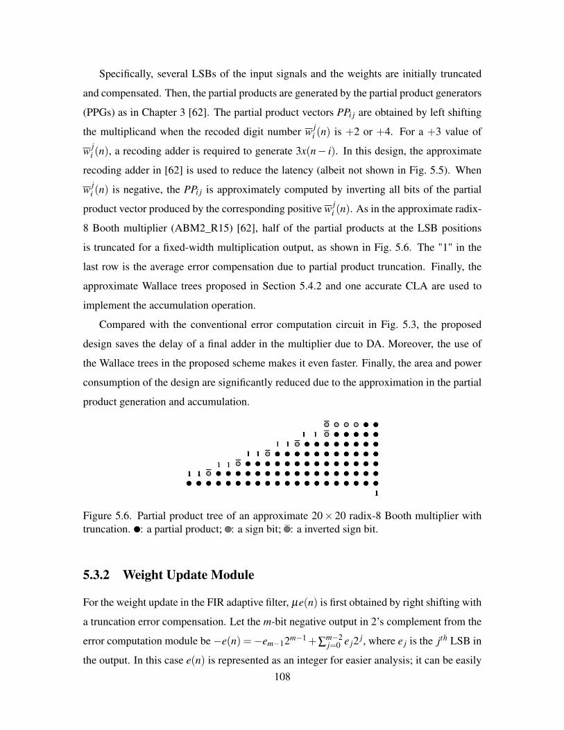
Specifically, several LSBs of the input signals and the weights are initially truncated

and compensated. Then, the partial products are generated by the partial product generators

(PPGs) as in Chapter 3 [62]. The partial product vectors PPi j are obtained by left shifting

the multiplicand when the recoded digit number w ji (n) is +2 or +4. For a +3 value of

w ji (n), a recoding adder is required to generate 3x(n− i). In this design, the approximate

recoding adder in [62] is used to reduce the latency (albeit not shown in Fig. 5.5). When

w ji (n) is negative, the PPi j is approximately computed by inverting all bits of the partial

product vector produced by the corresponding positive w ji (n). As in the approximate radix-

8 Booth multiplier (ABM2_R15) [62], half of the partial products at the LSB positions

is truncated for a fixed-width multiplication output, as shown in Fig. 5.6. The "1" in the

last row is the average error compensation due to partial product truncation. Finally, the

approximate Wallace trees proposed in Section 5.4.2 and one accurate CLA are used to

implement the accumulation operation.

Compared with the conventional error computation circuit in Fig. 5.3, the proposed

design saves the delay of a final adder in the multiplier due to DA. Moreover, the use of

the Wallace trees in the proposed scheme makes it even faster. Finally, the area and power

consumption of the design are significantly reduced due to the approximation in the partial

product generation and accumulation.

Figure 5.6. Partial product tree of an approximate 20× 20 radix-8 Booth multiplier withtruncation. : a partial product; : a sign bit; : a inverted sign bit.

5.3.2 Weight Update Module

For the weight update in the FIR adaptive filter, µe(n) is first obtained by right shifting with

a truncation error compensation. Let the m-bit negative output in 2’s complement from the

error computation module be−e(n) =−em−12m−1+∑m−2j=0 e j2 j, where e j is the jth LSB in

the output. In this case e(n) is represented as an integer for easier analysis; it can be easily108

transformed to a fixed-point format by shifting. If the step size µ for the weight update is

2−q and q is a positive integer, −µe(n) = −em−12m−q−1 +∑m−2j=0 e j2 j−q by right shifting

−e(n) by q bits. By truncating the q LSBs in the fractional part,−µe(n)≈−em−12m−q−1+

∑m−2j=q+1 e j2 j−q + 1 = (em−1 · · ·eq+2eq+11)2, where the "1" at the LSB position is the error

compensation for truncation. µe(n) is then obtained by a 2’s complement operation, i.e.,

µe(n) = (em−1 · · ·eq+2eq+11)2, where ei is the inverted value of ei, i = q+ 1, q+ 2, · · · ,

m− 1. After shifting and the 2’s complementing operation, µe(n) can be represented by

(m−q) bits by keeping one sign bit. Therefore, an (m−q)×m multiplication is sufficient

for computing each weight increment µe(n)x(n− i). Fig. 5.7 shows the partial product tree

based on an approximate Booth multiplier (ABM-R15) when m and q are 20 and 8, where

the partial products at the 19 LSB positions are truncated.

Figure 5.7. Partial product tree of an approximate 12× 20 radix-8 Booth multiplier withtruncation. : a partial product; : a sign bit; : a inverted sign bit.

Let v(n)= µe(n), and v(n)=−vm−q−1(n)2m−q−1+∑m−q−2j=0 v j(n)2 j in 2’s complement,

where v j(n) is the jth LSB of v(n). As per the radix-8 Booth algorithm, v(n) can be

represented as

v(n) =d(m−q)/3e−1

∑j=0

(−22v3 j+2(n)+2v3 j+1(n)+ v3 j(n)

+ v3 j−1(n))23 j =d(m−q)/3e−1

∑j=0

v j(n)23 j,

(5.11)

where v j(n) =−22v3 j+2(n)+2v3 j+1(n)+v3 j(n)+v3 j−1(n) is the radix-8 recoded number

in {−4, −3, −2, −1, 0, 1, 2, 3, 4}. According to (5.4), wi(n+1) is given by

wi(n+1) = v(n) · x(n− i)+wi(n) = [δ v,1] ·[

v(n) · x(n− i)wi(n)

], (5.12)

where δ v = [20, 23, · · · , 23d(m−q)/3e−3], and v(n) = [v0(n), v1(n), · · · , vd(m−q)/3e−1(n)]T .

Therefore, a (d(m−q)/3e+1)-input Wallace tree and a final m-bit adder are sufficient for

implementing the accumulation in (5.12).109

Fig. 5.8 shows the proposed weight update circuit; only one radix-8 Booth encoder is

required for the M multiplications because µe(n) is the same for the M weights. Also, the

recoding adders for calculating 3x(n− i) are shared with the ones in the error computation

module as they share the same input multiplicands ([x(n), x(n− 1), · · · , x(n−M + 1)]).

Similarly, a PPG is used to compute the partial product vectors v(n) · x(n− i). Then, the

partial product vectors and the weight at the former iteration wi(n) are accumulated by a

(d(m−q)/3e+1)-input Wallace tree. The new weight wi(n+1) is obtained by adding the

two output vectors of the Wallace tree using an m-bit CLA. As the weight update module

is more sensitive to errors, a smaller number of LSBs is approximated in the Wallace tree.

Radix-8 Booth

Encoder

μe(n)

D D D...x(n) x(n-M+1)x(n-1) x(n-2)

...

w0(n) w1(n) wM-1(n)w2(n) ...

w1(n+1) w2(n+1) wM-1(n+1)

Wallace Tree

PPG PPG PPG PPG

Wallace Tree

Wallace Tree

Wallace Tree

... ......

CLA CLA CLA

w0(n+1)

CLA

Figure 5.8. Proposed weight update scheme. PPG: the partial product generator; CLA: them-bit carry lookahead adder.

Consequently, the proposed weight update design saves (M − 1) radix-8 Booth

encoders and M recoding adders compared with a conventional multiplier based design. It

significantly reduces the area and power dissipation when M is large. Moreover, the

critical path delay of the proposed design is reduced by 2× of the delay of an adder (i.e.,

by the delays of the recoding adder and the final adder in the multiplication) compared

with the design in Fig. 5.4.

5.4 Truncated Partial Product Generation andApproximate Accumulation

To reduce area, power dissipation and critical path delay of the proposed design, the partial

products in DA are generated by truncating some LSBs of the inputs.

In a parallel DA architecture, accumulation is usually implemented by an adder tree.

As the carry-propagating adders in an adder tree are very slow, a Wallace tree is used in110

this design to speed up the accumulation stage. Moreover, the Wallace tree is approximated

to lower the power dissipation.

5.4.1 Truncated Partial Product Generation

Due to the partial product accumulation, the final result of an inner product will not be

significantly affected if the average error of the approximate partial products is small.

An m-bit number A in 2’s complement can be represented as

A =−am−12m−1 +∑m−2i=0 ai2i, where ai is the ith LSB of A, m is the bit width of A, and the

most significant bit am−1 is the sign bit. Let AH be the remaining value of A with k

(1 ≤ k ≤ m/2) LSBs truncated. Then, AH = −am−12m−1 + ∑m−2i=k ai2i. Let AL be

∑k−1i=0 ai2i, the truncation error is then AH −A = −AL. Let the probability of ai = 1 be p,

where 0≤ p≤ 1. The average error due to truncation is given by

E[−AL] =−pk−1

∑i=0

2i = p(1−2k), (5.13)

where E[·] denotes an expected value. The maximum error distance (in the absolute value

of the error) occurs when the k LSBs of A are all ones. So, the maximum error distance

(Dmax) of AH is

Dmax =k−1

∑i=0

2i = 2k−1. (5.14)

As per (5.13), the average error of a truncated number is approximately −2k p. To

compensate this error, 2k p is added to AH . Assume 0 and 1 are equally likely to occur, i.e.,

the probability of ai = 1 or ai = 0 is 2−1. In this case, the compensation error is 2k−1. The

compensated number A′ is given by

A′ = AH +2k−1 =−am−12m−1 +m−2

∑i=k−1

ai2i, (5.15)

where ak−1 is "1." In this case, truncation error becomes A′−A =−AL +2k−1; the average

error of the truncated number in (5.13) is reduced to E[−AL] + 2k−1 = 2−1. The Dmax

occurs when k LSBs of A are zeros; it is reduced to 2k−1. Using this error compensation

scheme for the truncated input operands, the average error of the partial products can be

computed in a signed multiplication. Assume that X = XH +XL and Y = YH +YL are the

111

multiplicand and multiplier, respectively, the average error of the partial products is then

given by

E[EPP] = E[(XH +2k−1)(YH +2k−1)− (XH +XL)(YH +YL)], (5.16)

where XH = −xm−12m−1 +∑m−2i=k xi2i, XL = ∑

k−1i=0 xi2i, YH = −ym−12m−1 +∑

m−2i=k yi2i and

YL = ∑k−1i=0 yi2i. When the probability of xi = 1 and yi = 1 is 0.5, E[XH ] = E[YH ] is

2−1(−2m−1 +∑m−2i=k 2i) =−2k−1, and E[XL] = E[YL] is 2k−1−2−1 as per (5.13). As X and

Y are independent, E[YHXL] = E[YH ]E[XL], E[XHYL] = E[XH ]E[YL] and

E[XLYL] = E[XL]E[YL]. The average error of the partial products in (5.16) becomes

E[EPP] = (2k−1(E[XH ]+E[YH ])+22k−2)

− (E[XH ]E[YL]+E[YH ]E[XL]+E[XL]E[YL])

=−2−2

. (5.17)

This result indicates that the number of partial products in a DA architecture can be

reduced by truncating some LSBs of the input data, and the accumulated sum can be rather

accurate by using the proposed error compensation scheme.

For a fixed-width implementation of DA, the partial products at the LSB positions can

be truncated as in the fixed-width multiplication. Thus, the partial product generation and

error compensation schemes for a fixed-width multiplier are further applied to the

proposed DA partial product generation. In the fixed-width multiplier design, the partial

products at the lower half bit positions are truncated, and the error is compensated by an

error compensation strategy. Several error compensation strategies have been proposed for

fixed-width Booth multipliers [28, 62, 84, 145]. Among them, the probabilistic [84] and

approximate recoding adder based approaches are very efficient and applicable to the

radix-8 Booth algorithm. The comparison in [62] shows that the approximate recoding

adder based scheme is significantly more accurate and hardware-efficient than the

probabilistic approach for a fixed-width radix-8 Booth multiplier.

In the proposed FIR adaptive filter, therefore, the m-bit input data are truncated by k

LSBs and compensated first. The partial products are then approximately generated using

the radix-8 Booth encoder and the PPG in the (m− k+ 1)× (m− k+ 1) ABM2-R15. To

assess the accuracy of the approximate partial product generation scheme for DA, the

112

inner product of a 64-dimensional vector pair is simulated. In this simulation, 5 LSBs of

the inputs are truncated and compensated. The inputs are five million combinations; each

combination consists of 64 16-bit random integers generated from the normal distribution.

The inputs are divided by 215 to ensure that the inputs are in the range of [−1,1) and in the

fixed-point representation with 1 sign bit and 15 fractional bits. The input combinations

for the simulation are selected to make sure their inner products are in the range of [−1,1).

Thus, the inner products are also represented by 16-bit fixed-point numbers with 1 sign bit

and 15 fractional bits. Errors are then computed as the difference between the approximate

results and the accurate results. To show the errors in integers, both the accurate and

approximate inner products are multiplied by 215. The simulation results show that about

99.79% of the errors are within (−400,400). Fig. 5.9 shows the distribution of the errors,

where the mean and standard deviation of the errors are around 4 and 122, respectively.

Since the range for the accurate outputs is [−32768,32767), the simulation results indicate

that most of the errors due to the approximate partial product generation are very small.

Figure 5.9. The error distribution of the proposed approximate partial product generationfor DA.

5.4.2 Approximate Accumulation

Fig. 5.10(a) and (b) show the structures of a traditional adder tree (AT) and a Wallace

tree (WT) for six m-bit inputs, respectively. For an AT, there are (M− 1) m-bit adders in

dlog2Me stages for M inputs (M > 2). Thus, the circuit area and the critical path delay

113

are CAT = (M− 1)×CmA and tAT = dlog2Me × tmA, where CmA and tmA are the circuit

area and critical path delay of an m-bit adder. However, the WT requires blog1.5Mc (for

M > 13; there is not a general formula to represent the number of required stages in a WT

for M≤ 13) carry-save stages and one final m-bit carry propagate adder for M inputs. Thus,

the circuit area and the critical path delay of the WT are CWT = (M−2)×m×CFA +CmA

and tWT = blog1.5Mc× tFA + tmA, where CFA and tFA are the circuit area and critical path

delay of a full adder [10]. It is evident that CAT ≥CWT when CmA≥m×CFA, and tAT > tWT

when tmA > log1.521−1/log2M × tFA. As log1.52

1−1/log2M decreases with the increase of M, a WT is more

efficient in delay than an AT when M is large. In an extreme case where M = 4, we have

tAT = 2× tmA and tWT = 2× tAF + tmA. Therefore, a WT is faster than an AT as long as

tmA > 2× tFA. For the RCA, CmA and tmA are proportional to m, while they are proportional

to log2m and mlog2m, respectively, for a fast CLA. Obviously, a WT has a similar size of

circuit with an AT when RCAs are used. On the other hand, a WT has a smaller circuit than

an AT when CLAs are used. Additionally, the speed of a WT can be improved by up to

30% by optimizing the signal connections among full adders using the algorithm in [124].

Thus, a speed-optimized WT is implemented for the parallel mode DA in the proposed FIR

adaptive filter design.

To further reduce circuit complexity, approximation is applied to the less significant

part of a WT as in the lower-part-OR adder (LOA) [101]. In the LOA, the less significant

bits are "added" by OR gates and an AND gate is used to generate a carry-in signal for the

more significant bits that are summed by a precise adder. LOA is an efficient approximate

adder for the accumulative operation due to its low average error [63]. Fig. 5.10(c) shows

an approximate Wallace tree (AWT), in which the less significant bits are accumulated by

3-input OR gates instead of full adders, and 2-input AND gates are used to generate the

carry bits for the more significant bits (that are accurately accumulated by full adders). The

number of approximate LSBs determines the accuracy of an AWT. Thus, by changing the

number of approximate LSBs, the AWT is configured into a circuit with variable accuracy.

As the number of "1"s in the intermediate results increases within a Wallace tree due to the

OR operation, it is more likely to generate an error in a later stage. Therefore, the last few

stages in a Wallace tree can be accurately accumulated by using full adders to ensure a high

accuracy.

114

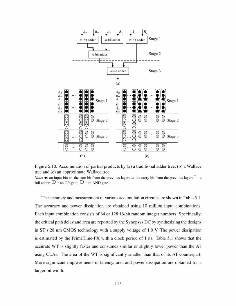
m-bit adder m-bit adder m-bit adder

m-bit adder

B0A0 B1A1 B2A2

m-bit adder

Stage 2

Stage 1

Stage 3

(a)

...

A0B0A1

B1A2B2

...

...

...

...

Stage 2

Stage 1

Stage 3

...

A0B0A1

B1A2B2

...

...

...

...

...

...

...

...

...

Stage 2

Stage 1

Stage 3

(b) (c)

Figure 5.10. Accumulation of partial products by (a) a traditional adder tree, (b) a Wallacetree and (c) an approximate Wallace tree.Note: : an input bit; : the sum bit from the previous layer; : the carry bit from the previous layer; : afull adder; : an OR gate; : an AND gate.

The accuracy and measurement of various accumulation circuits are shown in Table 5.1.

The accuracy and power dissipation are obtained using 10 million input combinations.

Each input combination consists of 64 or 128 16-bit random integer numbers. Specifically,

the critical path delay and area are reported by the Synopsys DC by synthesizing the designs

in ST’s 28 nm CMOS technology with a supply voltage of 1.0 V. The power dissipation

is estimated by the PrimeTime-PX with a clock period of 1 ns. Table 5.1 shows that the

accurate WT is slightly faster and consumes similar or slightly lower power than the AT

using CLAs. The area of the WT is significantly smaller than that of its AT counterpart.

More significant improvements in latency, area and power dissipation are obtained for a

larger bit width.

115

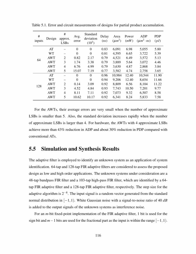
Table 5.1. Error and circuit measurements of designs for partial product accumulation.

#inputs

Design#

approx.LSBs

Avg.error

Standarddeviation

(103)

Delay(ns)

Area(µm2)

Power(mW )

ADP(µm2 ·ns)

PDP(pJ)

64

AT – 0 0 0.83 6,091 6.98 5,055 5.80WT – 0 0 0.81 4,595 6.65 3,722 5.39

AWT 2 0.82 2.17 0.79 4,521 6.49 3,572 5.13AWT 3 1.74 3.38 0.79 3,889 5.64 3,072 4.46AWT 4 6.76 4.99 0.79 3,630 4.87 2,868 3.84AWT 5 15.07 7.19 0.77 3,582 4.74 2,758 3.65

128

AT – 0 0 0.96 10,984 12.40 10,544 11.90WT – 0 0 0.94 9,206 12.40 8,654 11.66

AWT 2 0.14 3.09 0.92 8,809 6.56 8,104 11.22AWT 3 4.52 4.84 0.93 7,743 10.50 7,201 9.77AWT 4 8.11 7.11 0.92 7,073 9.32 6,507 8.58AWT 5 10.62 10.17 0.92 6,341 8.24 5,833 7.58

For the AWTs, their average errors are very small when the number of approximate

LSBs is smaller than 5. Also, the standard deviation increases rapidly when the number

of approximate LSBs is larger than 4. For hardware, the AWTs with 4 approximate LSBs

achieve more than 43% reduction in ADP and about 30% reduction in PDP compared with

conventional ATs.

5.5 Simulation and Synthesis Results

The adaptive filter is employed to identify an unknown system as an application of system

identification. 64-tap and 128-tap FIR adaptive filters are considered to assess the proposed

design as low and high order applications. The unknown systems under consideration are a

48-tap bandpass FIR filter and a 103-tap high-pass FIR filter, which are identified by a 64-

tap FIR adaptive filter and a 128-tap FIR adaptive filter, respectively. The step size for the

adaptive algorithm is 2−8. The input signal is a random vector generated from the standard

normal distribution in [−1,1). White Gaussian noise with a signal-to-noise ratio of 40 dB

is added to the output signals of the unknown systems as interference noise.

For an m-bit fixed-point implementation of the FIR adaptive filter, 1 bit is used for the

sign bit and m−1 bits are used for the fractional part as the input is within the range [−1,1).

116

5.5.1 Accuracy Evaluation

To evaluate the accuracy and convergence of the designs, the mean squared error (MSE) and

the normalized misalignment are considered. The MSE measures the difference between

the outputs of an unknown system and the adaptive filter. To show the performance in

convergence, the MSE is computed at each iteration of the algorithm. Considering the

variance in the MSE and computation time, the MSE is averaged over 20 independent trials

smoothed by a 20-point moving-average filter. The normalized misalignment indicates the

difference between an unknown system’s weights and the weights estimated by the adaptive

filter at each iteration. It is given by [81]

η(n) = 20log10‖h−w(n)‖‖h‖

, (5.18)

where ‖ · ‖ is the Euclidean norm operation, h is the weight vector of the unknown system,

and w(n) is the adaptive weight vector at the nth iteration.

Initially, the accurate direct-form FIR adaptive filters in Figs. 5.3 and 5.4 at different

resolutions (or bit widths) are simulated to investigate the effect of the resolution on

accuracy. For an m-bit implementation, the multiplication and addition are implemented

by an accurate m×m radix-8 Booth multiplier and an accurate m-bit CLA, respectively.

The 2m-bit product by an m×m multiplier is truncated and rounded to m-bit. For the

"unknown system" of a 48-tap FIR bandpass filter, Fig. 5.11 shows the impulse responses

of the identified systems using 20-bit, 16-bit, 14-bit and 12-bit fixed-point FIR adaptive

filters after 30,000 iterations. It can be seen that the results by the 12-bit and 14-bit

implementations are far off from the "unknown system", while the results by the 16-bit

and 20-bit implementations are more accurate due to the higher resolutions.

The learning curves in the MSE in Fig. 5.12(a) indicate that low resolution (e.g., 12-bit

and 14-bit) implementations converge more slowly to a higher steady-state MSE than high

resolution implementations. This occurs because an implementation with a higher

resolution retains more information of the processed data, which makes the learning

process more efficient than that with a lower resolution. The 16-bit implementation has a

similar learning curve in the MSE as the 20-bit implementation. However, the learning

curves in the normalized misalignment in Fig. 5.12(b) show that the weights obtained by

the 20-bit implementation are closer to those of the "unknown system". Similar results are117

0 0.5 1 1.5 2 2.5 3Angular frequency normalized by sampling frequency

-80

-60

-40

-20

0

Mag

nitu

de (d

B)

unknown system20-bit16-bit14-bit12-bit

Figure 5.11. The impulse responses of the identified systems by using accurate FIRadaptive filters at different resolutions.

0 10 20 30 40 50 60Number of iterations (× 512)

-45

-40

-35

-30

-25

-20

-15

Mea

n sq

uare

d er

ror (

dB)

20-bit16-bit14-bit12-bit

(a)

0 10 20 30 40 50 60Number of iterations (× 512)

-40

-30

-20

-10

0

Mis

alig

nmen

t (dB

)

20-bit16-bit14-bit12-bit

(b)

Figure 5.12. Learning curves of accurate FIR adaptive filters at different resolutions in (a)the mean squared error and (b) the normalized misalignment.

obtained for identifying a 103-tap FIR high-pass filter using accurate 128-tap FIR adaptive

filters at different resolutions, except that the difference in misalignment between the

16-bit and 20-bit implementations is larger.

Based on the comparison results of the accurate FIR adaptive filters, the 20-bit

implementation for the proposed FIR adaptive filter is selected to compare with the most

efficient DLMS-based designs in [106] at the same resolution. Four configurations of the

proposed design are considered for different numbers of truncated LSBs on the input data:

118

T0 (with no truncated bit), T5 (with 5 truncated LSBs), T7 (with 7 truncated LSBs) and

T9 (with 9 truncated LSBs). The simulation results in Table 5.1 show the tradeoff between

accuracy and hardware usage of the AWT. It shows that the AWT with 4 approximate

LSBs achieves the best tradeoff with a high accuracy and low power dissipation. Thus, in

the error computation module, 4 LSBs are approximated in the four least significant WTs,

and 2 LSBs are approximated in the two more significant WTs. The other Wallace trees

used in the proposed design remain accurate. For the DLMS design, the schemes without

pruning and with a pruning parameter of 11, referred to as DLMS (T0) and DLMS (T11),

are considered as well.

0 10 20 30 40 50 60Number of iterations ( × 512)

-40

-35

-30

-25

-20

-15

Mea

n sq

uare

d er

ror (

dB)

20-bit16-bit14-bitProposed (T0)Proposed (T5)Proposed (T7)Proposed (T9)

54 56 58

-40.5-40

-39.5-39

-38.5

(a)

0 10 20 30 40 50 60Number of iterations ( × 512)

-40

-35

-30

-25

-20

-15

Mea

n sq

uare

d er

ror (

dB)

DLMS (T0)DLMS (T11)Proposed (T0)Proposed (T5)Proposed (T7)Proposed (T9)

54 56 58

-40

-39

-38

(b)

Figure 5.13. Comparison of learning curves in the mean squared error between theproposed 64-tap adaptive filters and (a) accurate implementations and (b) DLMS-baseddesigns.

As shown in the learning curves for the 64-tap filters in Fig. 5.13, the proposed designs

have a similar convergence speed and steady-state MSE as the 20-bit and 16-bit accurate

designs. Compared with the DLMS design, the proposed designs converge slightly faster to

a lower MSE, as shown in Fig. 5.13(b). The normalized misalignment shown in Fig. 5.14

indicates that the proposed designs result in similar learning processes as the 20-bit accurate

design; these designs outperform the other considered designs. The DLMS design causes a

high misalignment, which indicates that the system weights identified by the DLMS design

are far from those of the actual system.

119

0 10 20 30 40 50 60Number of iterations ( × 512)

-45

-40

-35

-30

-25

-20

-15

-10

-5

0

5

Mis

alig

nmen

t (dB

)

20-bit16-bit14-bitDLMS (T0)DLMS (T11)Proposed (T0)Proposed (T5)Proposed (T7)Proposed (T9)

Figure 5.14. Learning curves in the normalized misalignment of 64-tap FIR adaptive filterdesigns.

0 10 20 30 40 50 60Number of iterations ( × 512)

-40

-35

-30

-25

-20

-15

Mea

n sq

uare

d er

ror (

dB)

20-bit16-bit14-bitProposed (T0)Proposed (T5)Proposed (T7)Proposed (T9)

54 56 58

-40

-39

-38

(a)

0 10 20 30 40 50 60Number of iterations ( × 512)

-40

-35

-30

-25

-20

-15

Mea

n sq

uare

d er

ror (

dB)

DLMS (T0)DLMS (T11)Proposed (T0)Proposed (T5)Proposed (T7)Proposed (T9)

56 58

-39.5-39

-38.5-38

(b)

Figure 5.15. Comparison of learning curves in the mean squared error between theproposed 128-tap adaptive filters and (a) accurate implementations and (b) DLMS-baseddesigns.

For the 128-tap FIR adaptive filter designs, the learning results are shown in Fig. 5.15.

As can be seen, the convergence speeds of the proposed T0 and T5 are slightly slower,

whereas the learning curves in the MSE for the T7 and T9 are similar to the accurate 20-

bit and 16-bit designs. Fig. 5.15(b) shows that the proposed designs (except for the T0)

perform better than the DLMS designs with lower steady-state MSEs. Similar learning

curves in the normalized misalignment are obtained for the 128-tap designs and shown in

120

0 10 20 30 40 50 60Number of iterations ( × 512)

-45

-40

-35

-30

-25

-20

-15

-10

-5

0

5

Mis

alig

nmen

t (dB

)

20-bit16-bit14-bitDLMS (T0)DLMS (T11)Proposed (T0)Proposed (T5)Proposed (T7)proposed (T9)

Figure 5.16. Learning curves in the normalized misalignment of 128-tap FIR adaptive filterdesigns.

Fig. 5.16. However, the differences between the proposed designs are rather noticeable. In

this case, the learning curves in the misalignment of T0 and T5 are closer to the accurate 16-

bit design, and the curves for T7 and T9 are closer to the accurate 20-bit design. Moreover,

the steady-state MSEs of the considered designs (reported in Table 5.2) show a similar

trend.

Table 5.2. Steady-state MSEs of considered FIR adaptive filter designs in an increasingorder (dB). prpsd.: proposed.

Filterlength

20-bit 16-bitprpsd.(T7)

prpsd.(T9)

prpsd.(T5)

prpsd.(T0)

14-bitDLMS

(T0)DLMS(T11)

64 -39.98 -39.86 -39.80 -39.78 -39.67 -38.59 -38.94 -39.53 -38.56128 -39.97 -39.85 -39.37 -39.32 -38.90 -38.40 -38.59 -38.21 -38.20

5.5.2 Hardware Efficiency

To evaluate the hardware efficiency, the filter designs are implemented in VHDL and

synthesized by the Synopsys DC in ST’s 28 nm CMOS technology. For ease of

comparison, all designs are synthesized in the same process with the same supply voltage,

temperature, optimization option and clock period. The supply voltage and temperature

are 1.0 V and 25 ◦C, respectively. The critical path delay and area of the designs are

reported by the Synopsys DC. The average power dissipation is estimated by using the

121

PrimeTime-PX with the same inputs as in the accuracy evaluation. The clock period for

the power estimation is 4 ns.

For the performance evaluation, the values of the energy per operation (EPO) and

throughput per area (TPA) are computed for the considered designs [147]. The EPO is

defined as the energy consumed per operation during one clock period, and the TPA is

defined as the number of operations per unit time and per unit area. They are respectively

given by

EPO = top×Power, (5.19)

and

T PA = 1/(tmin×Area), (5.20)

where top and tmin are respectively the time required per operation, i.e., the operating clock

period of a circuit, and the shortest time required per operation (or the critical path delay of

a combinational circuit). Power is the total power consumption including the dynamic and

leakage powers. Area is the circuit area.

Table 5.3 shows the hardware measurements of the FIR adaptive filter circuits. The

"shared-LUT" denotes an accurate 20-bit fixed-point implementation of the FIR adaptive

filter using shared LUTs (16-word) [127]; CLAs are used to implement the additions in

this design. For a fair comparison, in the other accurate implementations without using

DA (20-bit, 16-bit, 14-bit and 12-bit), the multiplications and additions are implemented

by radix-8 Booth multipliers and CLAs, respectively. The additions in the DLMS-based

design and the shared-LUT design are implemented by CLAs too. During the synthesis, the

shortest critical path delay is found such that the tightest timing constraint is applied to each

design with no timing violation. Table 5.3 shows that the shared-LUT design is the slowest

and that its improvements in area and power are very small compared to the accurate 20-

bit implementation. The long delay is mainly due to the update and access of the LUTs.

The DA architecture using LUTs is more efficient for an FIR filter with fixed coefficients,

for which no update is required for the LUTs. The hardware efficiency of the shared-LUT

design decreases with the increase of the filter length. The proposed designs require shorter

critical path delays than the accurate designs; however, the DLMS designs have the shortest

delays due to the pipelining implementation. Increasing the number of truncated LSBs on

the inputs has a more significant effect on reductions in area and power consumption than122

Table 5.3. Hardware characteristics of the FIR adaptive filter designs.

Filterlength

DesignDelay(ns)

Area(µm2)

Totalpower(mW )

Leakagepower(µW )

EPO(pJ/op.)

TPA(op.

/(s ·µm2)

EPOfall(%)

TPAup(%)

64

20-bit 2.78 246,472 85.3 191.6 341.2 1,459 0.00 0.0016-bit 2.73 222,021 78.4 171.8 313.6 1,650 8.09 13.0514-bit 2.67 214,142 75.4 172.9 301.6 1,749 11.61 19.8412-bit 2.65 193,616 67.6 154.7 270.4 1,949 20.75 33.54

DLMS (T0) 0.73 208,178 84.2 119.0 336.8 6,580 1.29 350.88DLMS (T11) 0.74 188,785 76.8 103.9 306.8 7,158 10.08 390.47shared-LUT 2.92 217,296 67.9 253.7 271.6 1,576 20.40 7.99

proposed (T0) 2.13 98,644 37.2 76.43 148.8 4,759 56.39 226.11proposed (T5) 2.13 93,897 35.5 74.27 142.0 5,000 58.39 242.60proposed (T7) 2.11 94,593 36.0 77.29 144.0 5,010 57.80 243.30proposed (T9) 2.11 84,577 32.8 67.61 131.2 5,604 61.55 283.95

128

20-bit 2.90 448,025 150.4 327.3 601.6 770 0.00 0.0016-bit 2.86 433,610 146.8 331.4 587.2 806 2.39 4.7714-bit 2.85 368,019 125.4 271.5 501.6 953 16.62 23.8812-bit 2.81 362,233 123.5 279.0 494.0 982 17.88 27.65

DLMS (T0) 0.77 384,163 154.3 207.2 617.2 3,380 -2.59 339.23DLMS (T11) 0.76 359,219 145.1 193.5 508.4 3,663 3.52 375.91shared-LUT 3.10 405,515 123.3 271.0 493.2 795 18.02 3.36

proposed (T0) 2.29 193,439 70.3 146.4 281.2 2,257 53.26 193.31proposed (T5) 2.27 184,281 67.4 141.1 269.6 2,391 55.19 210.59proposed (T7) 2.25 175,127 65.7 137.9 262.8 2,537 56.32 229.74proposed (T9) 2.24 170,672 63.7 134.8 254.8 2,615 57.65 239.85

Note: In the accurate implementations (20-bit, 16-bit, 14-bit and 12-bit), the multiplicationsand additions are implemented by radix-8 Booth multipliers and CLAs, respectively. Theadditions in the DLMS-based design and the shared-LUT design are implemented by CLAs.

on delay, because the critical path of the Wallace tree in the proposed design is very short

and reducing the accumulated partial product bits does not change it much. Among the

considered designs, the proposed designs require the lowest area and power dissipation.

The accurate designs incur the largest critical path delay, and the DLMS designs require

slightly smaller area than the accurate ones. Furthermore, the DLMS designs incur higher

power dissipations than some accurate designs due to the large hardware overhead caused

by the additional latches used for pipelining. The proposed designs show the lowest EPO,

whereas the DLMS designs require the highest EPO.

Finally, the EPO reduction and TPA increase of the filter designs are reported in the

last two columns of Table 5.3. The proposed designs achieve nearly a 55% EPO reduction

123

and a 3.2× TPA on average compared to the accurate 20-bit implementation. Additionally,

they show a 45%-51% reduction in EPO and 2.3× to 2.9× TPA compared with an accurate

12-bit implementation. The EPO of the DLMS designs is larger by 2%-9% due to the

high power dissipation. However, the TPAs are larger by 3.4× to 3.9× due to the shorter

critical path delay. Compared with DLMS designs, the proposed ones show lower TPAs

and smaller EPOs by 15%-38% and 45%-61%, respectively.

5.6 Cerebellar Model Evaluation

The cerebellum plays a key role in the control of eye movement in the saccadic system;

this involuntary eye movement is referred to as the vestibulo-ocular reflex (VOR). The

VOR stabilizes a visual stimulus into the center of the retina (fovea) for a clear vision

when the head moves [5]. Fig. 5.17 shows a simplified model of the VOR, where the

cerebellum predicts the eye plant output and indirectly compensates the movement

command. In the saccadic system, the head movements are sensed by the vestibular

system consisting of semicircular canals and otolith organs [131]. For simplicity, only the

horizontal head velocity sensed by the horizontal canal is considered as the input. The

horizontal canal is modeled as a high-pass filter, V (s) = ss+1/Tc

, where Tc = 6 s [131]. The

brainstem acts as a control center that receives the sensory information and compensation

signals from the cerebellum. It then generates commands to drive the eye muscles for

movement. The transfer functions of the brainstem and the eye plant are given by

B(s) = Gd +Gi

s+1/Tiand P(s) = s(s+1/Tz)

(s+1/T1)(s+1/T2), respectively, where Gd = 1, Gi = 5.05,

Ti = 500 ms, T1 = 370 ms, T2 = 57 ms and Tz = 200 ms [31].

∑ Brainstem

+Head

velocityEye

velocity

Cerebellar model

+Movement Command Eye

PlantVestibular

System

Retinal slip e(t)∑

+

-

Figure 5.17. A simplified model of the VOR.

124

To evaluate the accuracy of the approximate cerebellar model, the saccadic system in

Fig. 5.17 is implemented in MATLAB. The cerebellar model is implemented in an n-bit

fixed-point format consisting of 1 sign bit and (n− 1) fractional bits. Fig. 5.18 shows the

retinal slip (i.e., error signal) during a 5-s training, where the constant delay T is 1ms, M is

128, and the step size µ is set to 2−8. It can be seen that the accurate 20-bit fixed-point

cerebellar model produces the lowest stable retinal slip, followed by the 18-bit

implementation, whereas the retinal slip of the 16-bit implementation does not converge.

The proposed T0 and DLMS designs achieve a similarly small retinal slip as the accurate

20-bit design. However, the DLMS designs show more fluctuations than the proposed T0

at the stable phase, as shown in the inset. The proposed T5 converges faster than the other

designs, but it generates a similar retinal slip as the accurate 18-bit design that is slightly

larger than the accurate 20-bit design. As the VOR system requires a higher accuracy than

the system identification application, a converged retinal slip cannot be obtained by using

the other configurations of the proposed design.

0 0.5 1 1.5 2 2.5 3 3.5 4 4.5 5t (s)

-0.05

-0.04

-0.03

-0.02

-0.01

0

0.01

0.02

0.03

0.04

0.05

Ret

inal

Slip

(deg

/s)

Accurate (20-bit)Accurate (18-bit)Accurate (16-bit)DLMS (T0)DLMS (T11)Proposed (T0)Proposed (T5)

4.7 4.8 4.9-2

0

2

4

×10-3

Figure 5.18. The retinal slip during a 5-s VOR training.

5.7 Summary

This chapter presents a high-performance and energy-efficient fixed-point FIR adaptive

filter. It utilizes an integrated circuit implementation of an approximate DA, so it achieves

significant improvements in delay, area and power dissipation. The radix-8 Booth algorithm125

using an approximate recoding adder is applied to the DA. Moreover, approximate partial

product generation and accumulation schemes are proposed for the error computation and

weight update modules in the adaptive filter. The critical path and hardware complexity are

significantly reduced due to the use of approximate and distributed arithmetic.

Two system identification applications using 64-tap and 128-tap FIR adaptive filters are

considered to assess the quality of the proposed design. At a similar accuracy, the proposed

design consumes more than 55% lower EPO and achieves a 3.2× TPA compared with the

corresponding accurate design. Compared to a state-of-the-art design, the proposed design

achieves a 45%-61% reduction in EPO with a higher accuracy. A visual saccadic system

using the proposed approximate adaptive filter in a cerebellar model achieves a similar

retinal slip in vestibulo-ocular reflex as using an accurate filter. These results indicate

that approximate arithmetic circuits are applicable to integrated circuit designs for better

performance and energy efficiency.

126

Chapter 6

Conclusion and Future Work

6.1 Summary

This dissertation begins with a comparative evaluation of the approximate arithmetic

circuits that have appeared in the literature. Based on this evaluation, new approximate

designs for signed multiplication, unsigned division and square root operation are

proposed. A finite impulse response (FIR) adaptive filter using approximate distributed

arithmetic (DA) circuits is designed for high-performance and low-power operations.

In Chapter 2, the approximate designs of three basic arithmetic circuits, adders,

multipliers and dividers, are reviewed, evaluated and compared to provide guidelines for

the selection of an appropriate design for a specific application with particular

requirements. The comparison results show that truncation is an efficient scheme to

reduce the hardware overhead of an arithmetic circuit. Most of the approximate adders in

the literature are designed for a high-speed and low ER (e.g., 0.02% for CSA-5) by cutting

off the carry propagation chain. A truncated adder has a high ER (more than 90% when

the number of truncated bits is larger than or equal to 2); however, it consumes more than

20% smaller PDP than most approximate adders (except for LOA) for a similar MRED.

The performance of a truncated adder is not always higher than the other approximate

adders. Unlike the adder, a truncated multiplier is faster than most other approximate

multipliers, but with a higher power dissipation, at a similar MRED. As a result, a

truncated unsigned multiplier has a smaller PDP by 15% than most other approximate

unsigned multipliers (except for TAM1, TAM2 and ICM) for a given MRED. Conversely,

127

a truncated Booth multiplier has a more than 40% larger MRED than most other

approximate Booth multipliers (except for BM04) when a similar PDP is considered.

An approximate recoding adder with a high performance and low power is presented

in Chapter 3. Approximate radix-8 Booth multipliers are then designed for signed

multiplication by using the proposed recoding adder and a truncated Wallace tree. The

simulation results show that the proposed ABM1 achieves a 20% speed up with a MRED

of 0.04% compared with its corresponding accurate design. Compared to the other

approximate Booth multipliers, ABM1 is the most accurate design with the lowest ER,

NMED and MRED, but a relatively large PDP. ABM2_C15 is a design with a much lower

power dissipation and a moderate accuracy compared with the other fixed-width Booth

multipliers.

In Chapter 4, an adaptive approximation based on two pruning schemes is proposed

for the design of an unsigned divider and SQR circuit. A division/SQR operation is then

realized by using a reduced-width exact divider/SQR circuit and a shifter. Compared with

their corresponding accurate designs, the proposed approximate 16/8 divider with a

maximum error distance of 49 achieves 60% improvements in speed and power

consumption. The approximate 16-bit SQR circuit with a maximum error distance of 31 is

75% faster and consumes 80% less power. Moreover, the simulation and synthesis results

show that the proposed divider and SQR circuit outperform the other approximate designs,

as well as in three image processing applications.

In Chapter 5, a fixed-point FIR adaptive filter is proposed for using approximate DA

circuits. Specifically, the radix-8 Booth algorithm is used in DA to reduce the number of

partial products. Approximate partial product generation using input truncation and error

correction, and approximate partial product accumulation schemes are utilized for a high-

performance and low-power operation. The proposed approximate adaptive filter shows a

similar accuracy as an accurate design in applications of system identification and saccadic

control (where the adaptive filter works as a cerebellar model). Furthermore, the proposed

design achieves more than 50% reduction in EPO and 2.2× increase in TPA on average

compared with the accurate design.

128

6.2 Future Work

Although fixed-point arithmetic circuits are sufficient for many applications, floating-point

computations are crucial for more complex operations, such as the training in a deep

learning application, because floating-point arithmetic circuits have a higher accuracy and

dynamic range (can process a wider range of numbers) than its fixed-point counterpart

with the same bit width. However, floating-point operations consume a high energy with a

relatively low performance, which makes it less appealing in deep learning applications.

As errors can be self-compensated or tolerated in deep neural networks, approximate

floating-point circuits can be utilized in such applications to reduce the hardware cost

while maintaining a high dynamic range.

Compared to fixed-point operation, fewer approximate designs have been proposed for

floating-point operation. As the most power and area consuming module, the mantissa

multiplier is commonly approximated in an approximate floating-point multiplier

[16, 59, 153, 158]. Although the mantissa multipliers in these designs are simplified by

approximation, the conventional approximate mantissa multipliers still consume a

relatively high power and large area. For the floating-point addition, fewer approximate

designs have been proposed compared to the floating-point multiplication. No

approximate divider or SQR circuit has so far been proposed in the literature for

floating-point operation.

Therefore, approximate floating-point arithmetic circuits will be investigated in our

future work. As per the evaluation in Chapter 2, the hardware improvement of the

approximate arithmetic circuits is limited for a circuit simplification based approach.

Approximate floating-point arithmetic circuits will be devised based on the approximation

of algorithms. Moreover, the sequential floating-point arithmetic circuits using functional

iterative algorithms will be investigated, e.g., the divider based on the Newton-Raphson

algorithm [71, 146]. The objective is to avoid the use of traditional arithmetic circuits with

relatively high hardware overhead. Hence, larger improvements in performance and power

dissipation are expected to be achieved.

Additionally, to further evaluate an approximate arithmetic circuit, other error metrics

can be considered, such as the root-mean-square error (L2-norm). The statistical

129

distribution of error for an approximate design and related parameters such as the standard

deviation can also be investigated to estimate the error effects on different inputs. Finally,

the effectiveness and limitations of the error metrics will be studied for different

applications.

130

Bibliography

[1] Tinku Acharya and Ajoy K. Ray. Image processing: principles and applications.

John Wiley & Sons, 2005.

[2] James S. Albus. A theory of cerebellar function. Mathematical Biosciences,

10(1):25–61, 1971.

[3] Rustin W. Allred. Circuits, systems, and methods implementing approximations for

logarithm, inverse logarithm, and reciprocal, 2007. US Patent 7,171,435.

[4] Shaahin Angizi, Zhezhi He, Ronald F. DeMara, and Deliang Fan. Composite

spintronic accuracy-configurable adder for low power digital signal processing. In

ISQED, pages 391–396. IEEE, 2017.

[5] Marco Antonelli, Angel J. Duran, Eris Chinellato, and Angel P. Del Pobil. Adaptive

saccade controller inspired by the primates’ cerebellum. In 2015 IEEE International

Conference on Robotics and Automation (ICRA), pages 5048–5053. IEEE, 2015.

[6] Muhammad Kamran Ayub, Osman Hasan, and Muhammad Shafique. Statistical

error analysis for low power approximate adders. In ACM/EDAC/IEEE Design

Automation Conference (DAC), pages 1–6. IEEE, 2017.

[7] Dursun Baran, Mustafa Aktan, and Vojin G. Oklobdzija. Energy efficient

implementation of parallel CMOS multipliers with improved compressors. In

ACM/IEEE International Symposium on Low Power Electronics and Design, pages

147–152. ACM, 2010.

[8] Benjamin Barrois, Olivier Sentieys, and Daniel Menard. The hidden cost of

functional approximation against careful data sizing: a case study. In Proceedings

131

of the Conference on Design, Automation & Test in Europe, pages 181–186. IEEE,

2017.

[9] Kartikeya Bhardwaj, Pravin S. Mane, and Jorg Henkel. Power- and area-efficient

approximate Wallace tree multiplier for error-resilient systems. In ISQED, pages

263–269, March 2014.

[10] K.C. Bickerstaff, Earl E. Swartzlander, and Michael J. Schulte. Analysis of column

compression multipliers. In IEEE Symposium on Computer Arithmetic, pages 33–

39, 2001.

[11] Andrew D. Booth. A signed binary multiplication technique. The Quarterly Journal

of Mechanics and Applied Mathematics, 4(2):236–240, 1951.

[12] Hao Cai, You Wang, Lirida AB Naviner, Zhaohao Wang, and Weisheng Zhao.

Approximate computing in MOS/spintronic non-volatile full-adder. In International

Symposium on Nanoscale Architectures (NANOARCH), pages 203–208. IEEE, 2016.

[13] Thomas W. Calvert and Frank Meno. Neural systems modeling applied to the

cerebellum. IEEE Transactions on Systems, Man, and Cybernetics, (3):363–374,

1972.

[14] Vincent Camus, Jeremy Schlachter, and Christian Enz. Energy-efficient inexact

speculative adder with high performance and accuracy control. In IEEE

International Symposium on Circuits and Systems (ISCAS), pages 45–48, 2015.

[15] Vincent Camus, Jeremy Schlachter, and Christian Enz. A low-power carry cut-back

approximate adder with fixed-point implementation and floating-point precision. In

Proceedings of the 53rd Annual Design Automation Conference, page 127. ACM,

2016.

[16] Vincent Camus, Jeremy Schlachter, Christian Enz, Michael Gautschi, and Frank K.

Gurkaynak. Approximate 32-bit floating-point unit design with 53% power-area

product reduction. In European Solid-State Circuits Conference, pages 465–468,

2016.

132

[17] Maurus Cappa and V. Carl Hamacher. An augmented iterative array for high-speed

binary division. IEEE Transactions on Computers, 100(2):172–175, 1973.

[18] Jienan Chen and Jianhao Hu. Energy-efficient digital signal processing via voltage-

overscaling-based residue number system. IEEE Transactions on Very Large Scale

Integration (VLSI) Systems, 21(7):1322–1332, 2013.

[19] Linbin Chen, Jie Han, Weiqiang Liu, and Fabrizio Lombardi. Design of approximate

unsigned integer non-restoring divider for inexact computing. In Proceedings of the

25th edition on Great Lakes Symposium on VLSI, pages 51–56. ACM, 2015.

[20] Linbin Chen, Jie Han, Weiqiang Liu, and Fabrizio Lombardi. On the design of

approximate restoring dividers for error-tolerant applications. IEEE Transactions on

Computers, 65(8):2522–2533, 2016.

[21] Linbin Chen, Weiqiang Liu, Jie Han, Paolo A. Montuschi, and Fabrizio Lombardi.

Design, evaluation and application of approximate high-radix dividers. IEEE

Transactions on Multi-Scale Computing Systems, 2018.

[22] Linbin Chen, Fabrizio Lombardi, Paolo Montuschi, Jie Han, and Weiqiang Liu.

Design of approximate high-radix dividers by inexact binary signed-digit addition.

In Proceedings of the on Great Lakes Symposium on VLSI 2017, pages 293–298.

ACM, 2017.

[23] Tianshi Chen, Zidong Du, Ninghui Sun, Jia Wang, Chengyong Wu, Yunji Chen,

and Olivier Temam. Diannao: A small-footprint high-throughput accelerator for

ubiquitous machine-learning. In ACM Sigplan Notices, volume 49, pages 269–284,

2014.

[24] Yuan-Ho Chen and Tsin-Yuan Chang. A high-accuracy adaptive conditional-

probability estimator for fixed-width Booth multipliers. IEEE Trans. Circuits and

Systems I: Regular Papers, 59(3):594–603, 2012.

[25] Yuan-Ho Chen, Jyun-Neng Chen, Tsin-Yuan Chang, and Chih-Wen Lu. High-

throughput multistandard transform core supporting MPEG/H.264/VC-1 using

133

common sharing distributed arithmetic. IEEE Transactions on VLSI Systems,

22(3):463–474, 2014.

[26] Yuan-Ho Chen, Chung-Yi Li, and Tsin-Yuan Chang. Area-effective and power-

efficient fixed-width Booth multipliers using generalized probabilistic estimation

bias. IEEE Journal on Emerging and Selected Topics in Circuits and Systems,

1(3):277–288, 2011.

[27] Yunji Chen, Tao Luo, Shaoli Liu, Shijin Zhang, Liqiang He, Jia Wang, Ling Li,

Tianshi Chen, Zhiwei Xu, Ninghui Sun, et al. Dadiannao: A machine-learning

supercomputer. In IEEE/ACM International Symposium on Microarchitecture, pages

609–622, 2014.

[28] Kyung-Ju Cho, Kwang-Chul Lee, Jin-Gyun Chung, and Keshab K. Parhi. Design

of low-error fixed-width modified Booth multiplier. IEEE Transactions on VLSI

Systems, 12(5):522–531, 2004.

[29] Danilo Comminiello, Michele Scarpiniti, Luis A. Azpicueta-Ruiz, Jeronimo Arenas-

Garcia, and Aurelio Uncini. Functional link adaptive filters for nonlinear acoustic

echo cancellation. IEEE Transactions on Audio, Speech, and Language Processing,

21(7):1502–1512, 2013.

[30] S.R. Datla, M.A. Thornton, and D.W. Matula. A low power high performance radix-

4 approximate squaring circuit. In ASAP, pages 91–97, July 2009.

[31] Paul Dean, John Porrill, and James V. Stone. Visual awareness and the cerebellum:

possible role of decorrelation control. Progress in brain research, 144:61–75, 2004.

[32] Filter Design. Analysis tool (FDATool). Signal Processing Toolbox™, http://www.

mathworks. com/help/dsp/ref/fdatool. html, 2013.

[33] Feng Ding. Decomposition based fast least squares algorithm for output error

systems. Signal Processing, 93(5):1235–1242, 2013.

134

[34] Kai Du, P. Varman, and K. Mohanram. High performance reliable variable latency

carry select addition. In Design, Automation & Test in Europe Conference &

Exhibition (DATE), 2012, pages 1257–1262, March 2012.

[35] John C. Eccles. The cerebellum as a neuronal machine. Springer Science & Business

Media, 2013.

[36] Milos D. Ercegovac, Tomás Lang, J.M. Muller, and Arnaud Tisserand.

Reciprocation, square root, inverse square root, and some elementary functions using

small multipliers. IEEE Transactions on computers, 49(7):628–637, 2000.

[37] Hadi Esmaeilzadeh, Emily Blem, Renee St Amant, Karthikeyan Sankaralingam, and

Doug Burger. Dark silicon and the end of multicore scaling. In Annual International

Symposium on Computer Architecture (ISCA), pages 365–376. IEEE, 2011.

[38] Hadi Esmaeilzadeh, Adrian Sampson, Luis Ceze, and Doug Burger. Architecture

support for disciplined approximate programming. In ACM SIGPLAN Notices,

volume 47, pages 301–312. ACM, 2012.

[39] Jan Fandrianto. Algorithm for high speed shared radix 4 division and radix 4 square-

root. In Computer Arithmetic (ARITH), 1987 IEEE 8th Symposium on, pages 73–79.

IEEE, 1987.

[40] Farzad Farshchi, Muhammad Saeed Abrishami, and Sied Mehdi Fakhraie. New

approximate multiplier for low power digital signal processing. In CADS, pages

25–30. IEEE, October 2013.

[41] R. Fisher, S. Perkins, A. Walker, and E. Wolfart. Pixel division, 2003.

[42] Michael J. Flynn. On division by functional iteration. IEEE Transactions on

Computers, 100(8):702–706, 1970.

[43] M. Fujita. Adaptive filter model of the cerebellum. Biological cybernetics,

45(3):195–206, 1982.

135

[44] Masahiko Fujita. New supervised learning theory applied to cerebellar modeling for

suppression of variability of saccade end points. Neural computation, 25(6):1440–

1471, 2013.

[45] Masahiko Fujita. A theory of cerebellar cortex and adaptive motor control based on

two types of universal function approximation capability. Neural Networks, 75:173–

196, 2016.

[46] Z. Jason Geng and Claire L. McCullough. Missile control using fuzzy cerebellar

model arithmetic computer neural networks. Journal of guidance, control, and

dynamics, 20(3):557–565, 1997.

[47] Qing Guo, Karin Strauss, Luis Ceze, and Henrique S. Malvar. High-density image

storage using approximate memory cells. In ACM SIGPLAN Notices, volume 51,

pages 413–426, 2016.

[48] Rui Guo and Linda S. DeBrunner. Two high-performance adaptive filter

implementation schemes using distributed arithmetic. IEEE Transactions on Circuits

and Systems II: Express Briefs, 58(9):600–604, 2011.

[49] V. Gupta, D. Mohapatra, A. Raghunathan, and K. Roy. Low-power digital signal

processing using approximate adders. IEEE Trans. CAD, 32(1):124–137, January

2013.

[50] Jie Han. Introduction to approximate computing. In 2016 IEEE 34th VLSI Test

Symposium (VTS), pages 1–1. IEEE, 2016.

[51] Jie Han and Michael Orshansky. Approximate computing: An emerging paradigm

for energy-efficient design. In Test Symposium (ETS), 2013 18th IEEE European,

pages 1–6. IEEE, 2013.

[52] Nikos Hardavellas, Michael Ferdman, Babak Falsafi, and Anastasia Ailamaki.

Toward dark silicon in servers. IEEE Micro, 31(4):6–15, 2011.

[53] Soheil Hashemi, R. Bahar, and Sherief Reda. Drum: A dynamic range unbiased

multiplier for approximate applications. In Proceedings of the IEEE/ACM

136

International Conference on Computer-Aided Design, pages 418–425. IEEE Press,

2015.

[54] Soheil Hashemi, R. Bahar, and Sherief Reda. A low-power dynamic divider for

approximate applications. In Proceedings of the 53rd Annual Design Automation

Conference, page 105. ACM, 2016.

[55] Michael Hassul and Patricia D. Daniels. Cerebellar dynamics: the mossy fiber input.

IEEE Transactions on Bio-Medical Engineering, (5):449–456, 1977.

[56] J. Hidalgo, V. Moreno-Vergara, O. Oballe, A. Daza, MJ Martín-Vázquez, and

A. Gago. A radix-8 multiplier unit design for specific purpose. In XIII Conference

of Design of Circuits and Integrated Systems, volume 10, pages 1535–1546, 1998.

[57] Junjun Hu and Weikang Qian. A new approximate adder with low relative error

and correct sign calculation. In Design, Automation & Test in Europe Conference &

Exhibition, pages 1449–1454, 2015.

[58] Jiawei Huang, John Lach, and Gabriel Robins. A methodology for energy-quality

tradeoff using imprecise hardware. In Proceedings of the 49th ACM Annual Design

Automation Conference, pages 504–509, June 2012.

[59] Mohsen Imani, Daniel Peroni, and Tajana Rosing. CFPU: configurable floating point

multiplier for energy-efficient computing. In Proceedings of the 54th Annual Design

Automation Conference, 2017.

[60] Masao Ito. Neural design of the cerebellar motor control system. Brain research,

40(1):81–84, 1972.

[61] Manish Kumar Jaiswal and Nitin Chandrachoodan. FPGA-based high-performance

and scalable block LU decomposition architecture. IEEE Transactions on

Computers, 61(1):60–72, 2012.

[62] Honglan Jiang, Jie Han, Fei Qiao, and Fabrizio Lombardi. Approximate radix-

8 Booth multipliers for low-power and high-performance operation. IEEE

Transactions on Computers, 65(8):2638–2644, 2016.

137

[63] Honglan Jiang, Cong Liu, Leibo Liu, Fabrizio Lombardi, and Jie Han. A review,

classification, and comparative evaluation of approximate arithmetic circuits. ACM

Journal on Emerging Technologies in Computing Systems, 13(4):60, 2017.

[64] Honglan Jiang, Cong Liu, Fabrizio Lombardi, and Jie Han. High-performance

approximate unsigned multipliers with configurable error recovery. IEEE

Transactions on Circuits and Systems I, accepted for publication., 2018.

[65] Honglan Jiang, Cong Liu, Naman Maheshwari, Fabrizio Lombardi, and Jie Han.

A comparative evaluation of approximate multipliers. In IEEE/ACM International

Symposium on Nanoscale Architectures, pages 191–196, July 2016.

[66] Honglan Jiang, Leibo Liu, and Jie Han. An efficient hardware design for cerebellar

models using approximate circuits: special session paper. In Proceedings of the

Twelfth IEEE/ACM/IFIP International Conference on Hardware/Software Codesign

and System Synthesis Companion, page 31. ACM, 2017.

[67] Honglan Jiang, Chengkun Shen, Pieter Jonker, Fabrizio Lombardi, and Jie Han.

Adaptive filter design using stochastic circuits. In IEEE Computer Society Annual

Symposium on VLSI (ISVLSI), pages 122–127. IEEE, 2016.

[68] Peter Kabal. The stability of adaptive minimum mean square error equalizers using

delayed adjustment. IEEE Transactions on Communications, 31(3):430–432, 1983.

[69] Andrew B. Kahng and Seokhyeong Kang. Accuracy-configurable adder for

approximate arithmetic designs. In Proceedings of the 49th ACM Annual Design

Automation Conference, pages 820–825, June 2012.

[70] Marjan Karkooti, Joseph R. Cavallaro, and Chris Dick. FPGA implementation of

matrix inversion using QRD-RLS algorithm. In Asilomar Conference on Signals,

Systems, and Computers, pages 1625–1629, 2005.

[71] Alan H Karp, Peter Markstein, and Dennis Brzezinski. Floating point arithmetic unit

using modified newton-raphson technique for division and square root, May 7 1996.

US Patent 5,515,308.

138

[72] D. Kelly, B. Phillips, and S. Al-Sarawi. Approximate signed binary integer

multipliers for arithmetic data value speculation. In Conference on Design &

Architectures For Signal And Image Processing, Sophia Antipolis, France, 2009.

[73] Yongtae Kim, Yong Zhang, and Peng Li. An energy efficient approximate adder with

carry skip for error resilient neuromorphic vlsi systems. In ICCAD, pages 130–137,

November 2013.

[74] Eric J. King and E.E. Swartzlander. Data-dependent truncation scheme for parallel

multipliers. In Conference Record of the Thirty-First Asilomar Conference on

Signals, Systems &amp; Computers, volume 2, pages 1178–1182, 1997.

[75] E. Hari Krishna, M. Raghuram, K. Venu Madhav, and K. Ashoka Reddy. Acoustic

echo cancellation using a computationally efficient transform domain LMS adaptive

filter. In International Conference on Information Sciences Signal Processing and

their Applications, pages 409–412, 2010.

[76] Aravindh Krishnamoorthy and Deepak Menon. Matrix inversion using Cholesky

decomposition. In Signal Processing: Algorithms, Architectures, Arrangements,

and Applications, pages 70–72. IEEE, 2013.

[77] Parag Kulkarni, Puneet Gupta, and Milos Ercegovac. Trading accuracy for power

with an underdesigned multiplier architecture. In International Conference on VLSI

Design, pages 346–351, 2011.

[78] Khaing Yin Kyaw, Wang Ling Goh, and Kiat Seng Yeo. Low-power high-speed

multiplier for error-tolerant application. In EDSSC, pages 1–4, 2010.

[79] Jeanne Laine and Herbert Axelrad. The candelabrum cell: a new interneuron in the

cerebellar cortex. Journal of Comparative Neurology, 339(2):159–173, 1994.

[80] Mark SK Lau, Keck-Voon Ling, and Yun-Chung Chu. Energy-aware probabilistic

multiplier: design and analysis. In CASES, pages 281–290, 2009.

[81] Kong-Aik Lee, Woon-Seng Gan, and Sen M. Kuo. Subband adaptive filtering:

theory and implementation. John Wiley & Sons, 2009.

139

[82] Xinyu Lei, Xiaofeng Liao, Tingwen Huang, Huaqing Li, and Chunqiang Hu.

Outsourcing large matrix inversion computation to a public cloud. IEEE

Transactions on Cloud Computing, 1(1):78–87, 2013.

[83] Alexander Lenz, Sean R. Anderson, Anthony G. Pipe, Chris Melhuish, Paul Dean,

and John Porrill. Cerebellar-inspired adaptive control of a robot eye actuated by

pneumatic artificial muscles. IEEE Transactions on Systems, Man, and Cybernetics,

Part B (Cybernetics), 39(6):1420–1433, 2009.

[84] Chung-Yi Li, Yuan-Ho Chen, Tsin-Yuan Chang, and Jyun-Neng Chen. A

probabilistic estimation bias circuit for fixed-width Booth multiplier and its DCT

applications. IEEE Transactions on Circuits and Systems II: Express Briefs,

58(4):215–219, 2011.

[85] Li Li and Hai Zhou. On error modeling and analysis of approximate adders. In

ICCAD, pages 511–518, November 2014.

[86] Jinghang Liang, Jie Han, and F. Lombardi. New metrics for the reliability of

approximate and probabilistic adders. IEEE Trans. Comput., 62(9):1760–1771,

September 2013.

[87] Chia-Hao Lin and Ing-Chao Lin. High accuracy approximate multiplier with error

correction. In ICCD, pages 33–38. IEEE, October 2013.

[88] IngChao Lin, YiMing Yang, and ChengChian Lin. High-performance low-power

carry speculative addition with varible latency. IEEE Trans. VLSI Syst., 23(9):1591–

1603, 2015.

[89] Cong Liu. Design and analysis of approximate adders and multipliers. Master’s

thesis, University of Alberta, Canada, 2014.

[90] Cong Liu, Jie Han, and Fabrizio Lombardi. A low-power, high-performance

approximate multiplier with configurable partial error recovery. In Design,

Automation & Test in Europe Conference & Exhibition, pages 1–4, 2014.

140

[91] Cong Liu, Jie Han, and Fabrizio Lombardi. An analytical framework for evaluating

the error characteristics of approximate adders. IEEE Transactions on Computers,

64(5):1268–1281, 2015.

[92] Siting Liu and Jie Han. Hardware ode solvers using stochastic circuits. In

ACM/EDAC/IEEE Design Automation Conference (DAC), pages 1–6, 2017.

[93] Wei Liu and Alberto Nannarelli. Power efficient division and square root unit. IEEE

Transactions on Computers, 61(8):1059–1070, 2012.

[94] Weiqiang Liu, Liangyu Qian, Chenghua Wang, Honglan Jiang, Jie Han, and Fabrizio

Lombardi. Design of approximate radix-4 Booth multipliers for error-tolerant

computing. IEEE Transactions on Computers, 2017.

[95] Yang Liu, Tong Zhang, and Keshab K. Parhi. Computation error analysis in digital

signal processing systems with overscaled supply voltage. IEEE Transactions on

Very Large Scale Integration (VLSI) systems, 18(4):517–526, 2010.

[96] Guozhu Long, Fuyun Ling, and John G. Proakis. The LMS algorithm with

delayed coefficient adaptation. IEEE Transactions on Acoustics, Speech, and Signal

Processing, 37(9):1397–1405, 1989.

[97] Joshua Yung Lih Low and Ching Chuen Jong. Non-iterative high speed division

computation based on Mitchell logarithmic method. In IEEE International

Symposium on Circuits and Systems (ISCAS), pages 2219–2222, 2013.

[98] Shih-Lien Lu. Speeding up processing with approximation circuits. Computer,

37(3):67–73, March 2004.

[99] Jieming Ma, Ka Lok Man, Nan Zhang, Sheng-Uei Guan, and Taikyeong Ted Jeong.

High-speed area-efficient and power-aware multiplier design using approximate

compressors along with bottom-up tree topology. In ICMV: Algorithms, Pattern

Recognition, and Basic Technologies, 2013.

[100] Olin L. MacSorley. High-speed arithmetic in binary computers. Proceedings of the

IRE, 49(1):67–91, 1961.

141

[101] H.R. Mahdiani, A. Ahmadi, S.M. Fakhraie, and C. Lucas. Bio-inspired

imprecise computational blocks for efficient VLSI implementation of soft-

computing applications. IEEE Trans. Circuits and Systems, 57(4):850–862, April

2010.

[102] David Marr and W. Thomas Thach. A theory of cerebellar cortex. The Journal of

Physiology, 202(3):437–470, 1969.

[103] Maurizio Martina, Guido Masera, Massimo Ruo Roch, and Gianluca Piccinini.

Result-biased distributed-arithmetic-based filter architectures for approximately

computing the DWT. IEEE Transactions on Circuits and Systems I: Regular Papers,

62(8):2103–2113, 2015.

[104] Sana Mazahir, Osman Hasan, Rehan Hafiz, Muhammad Shafique, and Jörg Henkel.

Probabilistic error modeling for approximate adders. IEEE Transactions on

Computers, 66(3):515–530, 2017.

[105] Pramod Kumar Meher, Shrutisagar Chandrasekaran, and Abbes Amira. FPGA

realization of FIR filters by efficient and flexible systolization using distributed

arithmetic. IEEE Transactions on Signal Processing, 56(7):3009–3017, 2008.

[106] Pramod Kumar Meher and Sang Yoon Park. Area-delay-power efficient fixed-point

LMS adaptive filter with low adaptation-delay. IEEE Transactions on VLSI Systems,

22(2):362–371, 2014.

[107] Pramod Kumar Meher and Sang Yoon Park. Critical-path analysis and low-

complexity implementation of the LMS adaptive algorithm. IEEE Transactions on

Circuits and Systems I: Regular Papers, 61(3):778–788, 2014.

[108] Jin Miao, Ku He, Andreas Gerstlauer, and Michael Orshansky. Modeling and

synthesis of quality-energy optimal approximate adders. In Proceedings of the ACM

International Conference on Computer-Aided Design, pages 728–735, 2012.

[109] Joshua San Miguel, Jorge Albericio, Andreas Moshovos, and Natalie Enright Jerger.

Doppelgänger: a cache for approximate computing. In Proceedings of the 48th

International Symposium on Microarchitecture, pages 50–61. ACM, 2015.142

[110] Brian Millar, Philip E. Madrid, and E.E. Swartzlander. A fast hybrid multiplier

combining Booth and Wallace/Dadda algorithms. In Proceedings of the 35th

Midwest Symposium on Circuits and Systems, pages 158–165, 1992.

[111] SONG Min-An, VAN Lan-Da, and KUO Sy-Yen. Adaptive low-error fixed-

width Booth multipliers. IEICE Transactions on Fundamentals of Electronics,

Communications and Computer Sciences, 90(6):1180–1187, 2007.

[112] Shahnam Mirzaei, Anup Hosangadi, and Ryan Kastner. FPGA implementation of

high speed FIR filters using add and shift method. In International Conference on

Computer Design, pages 308–313, 2007.

[113] John N. Mitchell Jr. Computer multiplication and division using binary logarithms.

IRE Transactions on Electronic Computers, (4):512–517, 1962.

[114] Basant K. Mohanty and Pramod Kumar Meher. A high-performance energy-efficient

architecture for FIR adaptive filter based on new distributed arithmetic formulation

of block LMS algorithm. IEEE Transactions on Signal Processing, 61(4):921–932,

2013.

[115] D. Mohapatra, V.K. Chippa, A. Raghunathan, and K. Roy. Design of voltage-

scalable meta-functions for approximate computing. In Design, Automation & Test

in Europe Conference & Exhibition (DATE), pages 1–6, March 2011.

[116] Debabrata Mohapatra, Vinay K. Chippa, Anand Raghunathan, and Kaushik Roy.

Design of voltage-scalable meta-functions for approximate computing. In Design,

Automation & Test in Europe Conference & Exhibition (DATE), pages 1–6. IEEE,

2011.

[117] Amir Momeni, Jie Han, Paolo Montuschi, and Fabrizio Lombardi. Design and

analysis of approximate compressors for multiplication. IEEE Transactions on

Computers, 64(4):984–994, 2015.

[118] M. Monajati, Sied Mehdi Fakhraie, and E. Kabir. Approximate arithmetic for

low-power image median filtering. Circuits, Systems, and Signal Processing,

34(10):3191–3219, 2015.143

[119] Gordon E. Moore. Cramming more components onto integrated circuits.

Electronics, 38(8):114, 1965.

[120] Vojtech Mrazek, Syed Shakib Sarwar, Lukas Sekanina, Zdenek Vasicek, and

Kaushik Roy. Design of power-efficient approximate multipliers for approximate

artificial neural networks. In International Conference On Computer Aided Design

(ICCAD), page 7, 2016.

[121] Enrico Mugnaini and Alessandra Floris. The unipolar brush cell: a neglected

neuron of the mammalian cerebellar cortex. Journal of Comparative Neurology,

339(2):174–180, 1994.

[122] Ravi Nair. Big data needs approximate computing: technical perspective.

Communications of the ACM, 58(1):104–104, 2015.

[123] Srinivasan Narayanamoorthy, Hadi Asghari Moghaddam, Zhenhong Liu, Taejoon

Park, and Nam Sung Kim. Energy-efficient approximate multiplication for digital

signal processing and classification applications. IEEE Transactions on VLSI

Systems, 23(6):1180–1184, 2015.

[124] Vojin G. Oklobdzija, David Villeger, and Simon S. Liu. A method for speed

optimized partial product reduction and generation of fast parallel multipliers using

an algorithmic approach. IEEE Transactions on Computers, 45(3):294–306, 1996.

[125] Behrooz Parhami. Computer arithmetic. Oxford University Press, 2000.

[126] Behrooz Parhami. Computer Arithmetic: Algorithms and Hardware Designs, 2nd

edition. Oxford University Press, New York, 2010.

[127] Sang Yoon Park and Pramod Kumar Meher. Efficient FPGA and ASIC realizations

of da-based reconfigurable FIR digital filter. IEEE Transactions on Circuits and

Systems II: Express Briefs, 61(7):511–515, 2014.

[128] Thomas K. Paul and Tokunbo Ogunfunmi. On the convergence behavior of the affine

projection algorithm for adaptive filters. IEEE Transactions on Circuits and Systems

I: Regular Papers, 58(8):1813–1826, 2011.

144

[129] George Paxinos and Juergen K. Mai. The human nervous system. Academic Press,

2004.

[130] Amina Qureshi and Osman Hasan. Formal probabilistic analysis of low latency

approximate adders. IEEE Transactions on Computer-Aided Design of Integrated

Circuits and Systems, 2018.

[131] Mina Ranjbaran and Henrietta L. Galiana. Hybrid model of the context dependent

vestibulo-ocular reflex: implications for vergence-version interactions. Frontiers in

computational neuroscience, 9, 2015.

[132] Gholamali Rezai-Rad and Majid Aghababaie. Comparison of susan and sobel edge

detection in mri images for feature extraction. In Information and Communication

Technologies, 2006. ICTTA’06. 2nd, volume 1, pages 1103–1107. IEEE, 2006.

[133] Adrian Sampson, Werner Dietl, Emily Fortuna, Danushen Gnanapragasam, Luis

Ceze, and Dan Grossman. EnerJ: Approximate data types for safe and general low-

power computation. ACM SIGPLAN Notices, 46(6):164–174, June 2011.

[134] Muhammad Shafique, Siddharth Garg, Jörg Henkel, and Diana Marculescu. The

eda challenges in the dark silicon era: Temperature, reliability, and variability

perspectives. In Proceedings of the 51st Annual Design Automation Conference,

pages 1–6. ACM, 2014.

[135] Doochul Shin. Approximate logic synthesis for error tolerant applications. In

Design, Automation & Test in Europe Conference & Exhibition, pages 957–960.

IEEE, March 2010.

[136] Chitranjan K. Singh, Sushma Honnavara Prasad, and Poras T. Balsara. VLSI

architecture for matrix inversion using modified Gram-Schmidt based QR

decomposition. In VLSI Design, pages 836–841, 2007.

[137] Anton Spanne and Henrik Jörntell. Processing of multi-dimensional sensorimotor

information in the spinal and cerebellar neuronal circuitry: a new hypothesis. PLoS

Comput Biol, 9(3):e1002979, 2013.

145

[138] Jerome L. Stanislaus and T. Mohsenin. High performance compressive sensing

reconstruction hardware with QRD process. In IEEE International Symposium on

Circuits and Systems, pages 29–32, 2012.

[139] Nitish V. Thakor and Yi-Sheng Zhu. Applications of adaptive filtering to ECG

analysis: noise cancellation and arrhythmia detection. IEEE Transactions on

Biomedical Engineering, 38(8):785–794, 1991.

[140] Zdenek Vasicek and Lukas Sekanina. Evolutionary approach to approximate digital

circuits design. IEEE Transactions on Evolutionary Computation, 19(3):432–444,

2015.

[141] Swagath Venkataramani, Srimat T. Chakradhar, Kaushik Roy, and Anand

Raghunathan. Approximate computing and the quest for computing efficiency. In

Proceedings of the 52nd Annual Design Automation Conference, page 120. ACM,

2015.

[142] Swagath Venkataramani, Amit Sabne, Vivek Kozhikkottu, Kaushik Roy, and Anand

Raghunathan. SALSA: systematic logic synthesis of approximate circuits. In

Proceedings of the 49th Annual Design Automation Conference, pages 796–801.

ACM, 2012.

[143] Rangharajan Venkatesan, Amit Agarwal, Kaushik Roy, and Anand Raghunathan.

MACACO: Modeling and analysis of circuits for approximate computing. In

ICCAD, pages 667–673, November 2010.

[144] Ajay K. Verma, Philip Brisk, and Paolo Ienne. Variable latency speculative addition:

A new paradigm for arithmetic circuit design. In Design, Automation & Test in

Europe Conference & Exhibition, pages 1250–1255, March 2008.

[145] Jiun-Ping Wang, Shiann-Rong Kuang, and Shish-Chang Liang. High-accuracy

fixed-width modified Booth multipliers for lossy applications. IEEE Transactions

on VLSI Systems, 19(1):52–60, 2011.

146

[146] Liang-Kai Wang and Michael J. Schulte. Processing unit having decimal floating-

point divider using Newton-Raphson iteration, December 16 2008. US Patent

7,467,174.

[147] Ran Wang, Jie Han, Bruce Cockburn, and Duncan Elliott. Stochastic circuit design

and performance evaluation of vector quantization for different error measures. IEEE

Transactions on VLSI Systems, 24(10):3169–3183, 2016.

[148] Stanley A. White. Applications of distributed arithmetic to digital signal processing:

A tutorial review. IEEE Assp Magazine, 6(3):4–19, 1989.

[149] Lei Wu and Ching Chuen Jong. A curve fitting approach for non-iterative divider

design with accuracy and performance trade-off. In IEEE 13th International New

Circuits and Systems Conference (NEWCAS), pages 1–4, 2015.

[150] Xinghua Yang, Yue Xing, Fei Qiao, Qi Wei, and Huazhong Yang. Approximate

adder with hybrid prediction and error compensation technique. In IEEE Computer

Society Annual Symposium on VLSI (ISVLSI), pages 373–378. IEEE, 2016.

[151] Zhixi Yang, Ajaypat Jain, Jinghang Liang, Jie Han, and Fabrizio Lombardi.

Approximate XOR/XNOR-based adders for inexact computing. In IEEE-NANO,

pages 690–693, August 2013.

[152] Rong Ye, Ting Wang, Feng Yuan, Rakesh Kumar, and Qiang Xu. On

reconfiguration-oriented approximate adder design and its application. In ICCAD,

pages 48–54, November 2013.

[153] Peipei Yin, Chenghua Wang, Weiqiang Liu, Earl E. Swartzlander, and Fabrizio

Lombardi. Designs of approximate floating-point multipliers with variable accuracy

for error-tolerant applications. Journal of Signal Processing Systems, pages 1–14,

2017.

[154] Heejong Yoo and David V. Anderson. Hardware-efficient distributed arithmetic

architecture for high-order digital filters. In IEEE International Conference on

Acoustics, Speech, and Signal Processing, volume 5, pages 125–128, 2005.

147

[155] Xin Yuan and Raziel Haimi-Cohen. Image compression based on compressive

sensing: End-to-end comparison with JPEG. arXiv preprint arXiv:1706.01000,

2017.

[156] Reza Zendegani, Mehdi Kamal, Milad Bahadori, Ali Afzali-Kusha, and Massoud

Pedram. RoBA multiplier: A rounding-based approximate multiplier for high-speed

yet energy-efficient digital signal processing. IEEE Transactions on Very Large

Scale Integration (VLSI) Systems, 25(2):393–401, 2017.

[157] Reza Zendegani, Mehdi Kamal, Arash Fayyazi, Ali Afzali-Kusha, Saeed Safari,

and Massoud Pedram. SEERAD: a high speed yet energy-efficient rounding-

based approximate divider. In Design, Automation & Test in Europe Conference

& Exhibition (DATE), pages 1481–1484. IEEE, 2016.

[158] Hang Zhang, Wei Zhang, and John Lach. A low-power accuracy-configurable

floating point multiplier. In IEEE International Conference on Computer Design

(ICCD), pages 48–54. IEEE, 2014.

[159] Ning Zhu, Wang Ling Goh, and Kiat Seng Yeo. An enhanced low-power high-speed

adder for error-tolerant application. In ISIC 2009, pages 69–72, December 2009.

[160] Peican Zhu, Yangming Guo, Fabrizio Lombardi, and Jie Han. Approximate

reliability of multi-state two-terminal networks by stochastic analysis. IET

Networks, 6(5):116–124, 2017.

148

Appendix

Journal Publications

1. H. Jiang, C. Liu, L. Liu, F. Lombardi, and J. Han, "A review, classification, and

comparative evaluation of approximate arithmetic circuits," ACM Journal on

Emerging Technologies in Computing Systems, 13 (4), p. 60, 2017.

2. H. Jiang, J. Han, F. Qiao, and F. Lombardi, "Approximate radix-8 Booth multipliers for

low-power and high-performance operation," IEEE Transactions on Computers, 65(8):

2638–2644, 2016.

3. W. Liu, L. Qian, C. Wang, H. Jiang, J. Han, and F. Lombardi, "Design of approximate

radix-4 Booth multipliers for error-tolerant computing," IEEE Transactions on

Computers, 66(8): 1435–1441, 2017.

4. H. Jiang, L. Liu, P. Jonker, D. Elliott, F. Lombardi, and J. Han, "A High-Performance

and Energy-Efficient FIR Adaptive Filter using Approximate Distributed Arithmetic

Circuits," IEEE Transactions on Circuits and Systems I: Regular Papers, accepted for

publication, 14 pages, 2018.

5. H. Jiang, C. Liu, F. Lombardi and J. Han, "Low-Power Approximate Unsigned

Multipliers with Configurable Error Recovery," IEEE Transactions on Circuits and

Systems I: Regular Papers, accepted for publication, 14 pages, 2018.

6. S. Angizi, H. Jiang, R. F. DeMara, J. Han, and D. Fan, "Majority-Based Spin-CMOS

Primitives for Approximate Computing," IEEE Transactions on Nanotechnology, 17(4):

795-806, 2018.

149

7. M. S. Ansari, H. Jiang, B. F. Cockburn, J. Han, "Low-Power Approximate Multipliers

Using Encoded Partial Products and Approximate Compressors," IEEE Journal on

Emerging and Selected Topics in Circuits and Systems, accepted for publication, 13

pages, 2018.

8. S. Liu, H. Jiang, L. Liu, and J. Han, "Gradient Descent using Stochastic Circuits for

Efficient Training of Learning Machines," IEEE Transactions on Computer-Aided

Design of Integrated Circuits and Systems, accepted for publication, 12 pages, 2018.

9. V. Mrazek, Z. Vasicek, L. Sekanina, H. Jiang, and J. Han, "Scalable Construction of

Approximate Multipliers with Formally Guaranteed Worst-Case Error," IEEE

Transactions on Very Large Scale Integration Systems, accepted for publication, 5

pages, 2018.

Conference Publications

1. H. Jiang, L. Liu, F. Lombardi and J. Han, "Adaptive Approximation in Arithmetic

Circuits: A Low-Power Unsigned Divider Design," in Design, Automation & Test in

Europe Conference & Exhibition (DATE), pp. 1411-1416, Dresden, Germany, 2018.

2. H. Jiang, L. Liu, and J. Han, "An Efficient Hardware Design for Cerebellar Models

using Approximate Circuits: special session paper," in ACM/IEEE Conf.

Hardware/Software Co-design and System Synthesis (CODES/ISSS), p. 31, Seoul,

South Korea, 2017.

3. H. Jiang, C. Shen, P. Jonker, F. Lombardi, and J. Han, "Adaptive filter design using

stochastic circuit," in proceedings of IEEE Symposium on VLSI (ISVLSI), pp. 122-

127, Pittsburgh, PA, USA, 2016.

4. H. Jiang, Cong Liu, Naman Maheshwari, Fabrizio Lombardi, and Jie Han, "A

comparative evaluation of approximate multipliers," in IEEE/ACM International

Symposium on Nanoscale architectures (NanoArch), pp. 191-196, Beijing, China,

2016. (Best Paper Nomination)

150

5. H. Jiang, J. Han, and F. Lombardi, "A comparative review and evaluation of

approximate adders," in Proceedings of ACM Great Lakes Symposium on VLSI, pp.

343–348, Pittsburgh, PA, USA, 2015.

151