A constrained, total-variation minimization algorithm for

low-intensity X-ray CT

Emil Y. Sidky,∗ Yuval Duchin, and Xiaochuan Pan†

University of Chicago

Department of Radiology

5841 S. Maryland Ave.,

Chicago IL, 60637

Christer Ullberg

XCounter AB

Svardvagen 11

SE-182 33 Danderyd, Sweden

(Dated: December 30, 2013)

1

arX

iv:1

011.

4630

v1 [

phys

ics.

med

-ph]

21

Nov

201

0

Abstract

PURPOSE:

We develop an iterative image-reconstruction algorithm for application to low-intensity computed

tomography (CT) projection data, which is based on constrained, total-variation (TV) minimiza-

tion. The algorithm design focuses on recovering structure on length scales comparable to a

detector-bin width.

METHOD:

Recovering the resolution on the scale of a detector bin, requires that pixel size be much smaller

than the bin width. The resulting image array contains many more pixels than data, and this

undersampling is overcome with a combination of Fourier upsampling of each projection and the

use of constrained, TV-minimization, as suggested by compressive sensing. The presented pseudo-

code for solving constrained, TV-minimization is designed to yield an accurate solution to this

optimization problem within 100 iterations.

RESULTS:

The proposed image-reconstruction algorithm is applied to a low-intensity scan of a rabbit with

a thin wire, to test resolution. The proposed algorithm is compared with filtered back-projection

(FBP).

CONCLUSION:

The algorithm may have some advantage over FBP in that the resulting noise-level is lowered at

equivalent contrast levels of the wire.

∗Electronic address: sidky@uchicago.edu†Electronic address: xpan@uchicago.edu

2

I. INTRODUCTION

Motivated by the desire to reduce dose [1] and the ever-climbing availability of cheap

computation power, much effort has been directed to developing iterative image reconstruc-

tion (IIR) for application in X-ray CT [2–4]. When considering a fixed total X-ray dose for

a given scan, there is a trade-off between intensity-per-view and number-of-views. Much

of the recent work on IIR based on a constrained, `1 or total variation (TV) optimiza-

tion problem has explored the sparse-view end of this trade-off [4–11, 11–14]. While the

low-intensity/many-views end of this spectrum is generally dealt with by employing filtered

back-projection (FBP) with regularization or IIR based on a maximum-likelihood principle.

In this work, we would like to extend IIR based on constrained, TV-minimization to handle

CT data with many projections and low-intensity (high-noise) per projection.

The use of constrained, TV-minimization derives from recent theory in compressive sens-

ing (CS) [15–17], where certain sparsely sampled linear systems can be inverted accurately

when the underlying object has an approximately sparse gradient-magnitude image. The

CS-motivated optimization problem appears to be effective for accurate image reconstruc-

tion from sparse-view data as evaluated by many image quality metrics [18]. The obvious

question, now, is why would we want to extend constrained, TV-minimization to CT data

with many projections? The answer is that no matter how many projections a CT data

set contains, there may always be an issue with view-angle under-sampling. Particularly

in diagnostic X-ray CT, the bar for image quality is quite high; it is often expected that

detail on the scale of a single detector bin (0.1-0.25 mm) will be visible. At such scales,

images of structures are often degraded due to the fact that standard CT scans – even

with 1000 projections – contain too few views. Further evidence of under-sampling in CT

practice is that industry has developed a hardware solution, which is a X-ray source with

a flying focal-spot to effectively double the number of projections [19, 20]. By developing

constrained, TV-minimization for low-intensity/many-view data, we seek a software solution

to this problem. The technical problem to be overcome is how to effectively deal with noisy

projection data in the resulting IIR algorithm.

The main goal of this article is to report a constrained, TV-minimization IIR algorithm

for low-intensity/many-view CT projection data. The algorithm is derived from a framework

we have been developing where constrained, TV-minimization is solved with a combination

3

of steepest-descent (SD), to reduce image TV, and projection onto convex sets (POCS), to

enforce data-error and other image constraints. As the step-size of the SD component of

the algorithm is adaptively adjusted, the algorithm framework is referred to as adaptive

SD-POCS (ASD-POCS). The particular flavor of ASD-POCS presented here is designed to

solve constrained, TV-minimization accurately in a reasonable number of iterations ( 100

iterations). This ASD-POCS algorithm is demonstrated with an XCounter CT scan of a

rabbit with a thin wire taped to the outside of the sample holder. The data are low-intensity

and contain 1878 projections with a 2266x64 bin detector at a resolution of 0.1 mm. The

thin wire provides a good test for the image reconstruction algorithm. For our purpose,

we take the middle row on the detector from this data set and focus on 2D fan-beam CT

reconstruction with 1878 projections on a 2266-bin linear detector array. In Sec. II we

discuss in detail a fundamental issue of sampling for IIR; in Sec. III we present the ASD-

POCS algorithm for low-intensity CT; and in Sec. IV the algorithm is applied to the rabbit

scan.

II. SAMPLING AND IMAGE REPRESENTATION FOR HIGH-RESOLUTION

CT IMAGING

For FBP, which is an analytic-inverse-based image reconstruction algorithm, the data

sampling requirements are guided by the fact one needs a good estimate of the continuous

projection data. Whether done explicitly or not, the discretely sampled X-ray transform

is interpolated to a continuous function, then fed into an analytic-inverse formula for the

X-ray transform. In the theory for CT sampling, there is much discussion about satisfy-

ing a Nyquist sampling condition for the data, but in practice this condition is used only

as an estimate of resolution for a given CT system. Often objects being scanned in CT

have edge-discontinuities, which violate the band-limited requirement of Nyquist sampling.

Furthermore, most implementations of FBP use linear-interpolation in the filtering and back-

projection integrals instead of the sinc-interpolation called for by the sampling theorem. In

any case, the CT sampling issue boils down to how well the interpolated data function

matches the continuous projection of the underlying object function. The FBP image can

be displayed on a grid of any size, because FBP provides a closed-form expression for the

image in terms of the data. The accuracy of this image, however, depends on the accuracy

4

of the interpolation of the data function.

For IIR, which uses a discrete data model, the image resolution depends on two things:

(1) the expansion set used to represent the image, and (2) the number of measurements

available to determine the expansion coefficients. The first step is to design an expansion

set for the underlying object function. For the present work, we choose image pixels as

this expansion set. Fixing the expansion set, the next step to understanding the sampling

is to determine if there are enough ray-integration measurements to specify the expansion

coefficients. The required amount of data to determine a unique image depends on the

number of expansion elements. To explain this sampling issue for IIR more concretely, we

use the configuration of the XCounter CT of a rabbit-plus-wire.

The projection of the rabbit is confined to the middle 1266 bins of the detector so the

data size is effectively 1878 views by 1266 bins with each bin measuring 0.1 mm in width.

We would like to resolve structure within a (0.1 mm)2 region, and as a result the pixels

representing the image must be much smaller than this 0.1 mm square [21]. Say we choose

pixels of size 0.025 mm so that the 0.1 mm square has 16 sub-elements. It turns out the the

support of the rabbit can be covered by a 4096x4096 array of pixels of size (0.025 mm)2.

With this choice of parameters, the number of pixels is much larger than the number of

measurements. If instead we had decided to use (0.1 mm)2 pixels, the discrete data model

would not be an under-determined linear system. It is clear, however, that the data model

will always be under-determined if the pixel-size is chosen to be smaller than the detector

bin width. Using alternative basis functions does not resolve this dilemma; whenever it

is desirable to recover structure on the scale of a detector bin, there will be many more

expansion elements than measurements.

Within the framework of optimization-based image reconstruction, such under-sampling

problems are resolved by the exploitation of some kind of prior knowledge. One possible

choice is to exploit sparsity in the gradient magnitude image, and employ constrained, TV-

minimization. Mathematically, the constraints of having to agree with the data and image

non-negativity yields a multiplicity of images. But there will in general be one image, with in

this feasible sub-set, that has a minimum image TV. While constrained, TV-minimization

has proved useful for angular under-sampling, it may not be as effective when both the

scanning angle and detector bin direction are under-sampled, as is the case here.

A possible solution to the problem of how to employ a super-resolution grid of pixels

5

comes from analyzing the sampling for FBP. CT sampling is not uniform and the limiting

factor is usually the angular sampling rate. As a prior on the system, we can assume

that the sampling along the projection does satisfy the Nyquist sampling condition. If

this is the case, we can generate more samples by Fourier interpolation, zero-padding the

projection’s Fourier transform, to augment the data set to 1878 views by 5064 (4×1266) bins.

With this set of data, we are no longer undersampled on the direction along the detector.

Now, we can exploit sparsity in the gradient magnitude image, by basing the IIR algorithm

on constrained, TV-minimization. And we can expect this strategy to be successful, as

constrained, TV-minimization has been demonstrated to be effective against angular under-

sampling. Although, we have chosen a factor of 4, the method can be extended to even

larger sub-sampling factors because, under the assumption of Nyquist sampling along the

detector, the number of samples per projection can scale with the pixel grid size. Another

extension of this idea is to use other methods to interpolated the projections, for example,

linear interpolation.

III. THE ASD-POCS ALGORITHM FOR LOW-INTENSITY CT

Up until now, we have not addressed the issue of the high noise-level at each projection.

In this work, we do not explicitly incorporate a noise model into the design of the IIR

algorithm. Instead the consideration of noise is more of a practical issue in that it turns

out to be difficult to solve the constrained, TV-minimization problem with a large number

of views and a high noise level per view. The specific data model for our system is a linear

equation:

g = X ~f, (1)

where g represents the augmented projection data, in this case a vector of length 1878×5064;

~f is a vector of pixel values on the super-resolution grid, here 4096 × 4096; and X is the

ray-driven model of the X-ray transform where system matrix element is the intersection

length of a given ray through a given pixel. An IIR algorithm based on constrained, TV-

minimization aims at solving:

~f ∗ = argmin‖~f‖TV such that |X ~f − g|2 ≤ ε2 ~f ≥ 0, (2)

6

where ‖~f‖TV is the sum over the gradient magnitude image; and ε is a data-error tolerance

parameter. Because there will be no image that exactly reproduces the data, due to noise

and other physical factors, there will be a non-zero minimum data-error tolerance εmin. This

optimization problem can be difficult to solve for our system; especially, because we are

interested in values of ε near εmin. An IIR algorithm, however, can be designed to solve

this problem efficiently by converting Eq. (2) to an equivalent least-absolute-shrinkage-and-

selection-operator (LASSO) optimization problem [22].

In the LASSO form, the term representing the data error goes into the objective function

and the image TV is swapped out as a constraint:

~f ∗ = argmin|X ~f − g|2 such that ‖~f‖TV ≤ t0 ~f ≥ 0, (3)

where the parameter t0 is the maximum allowed image TV. This parameter replaces the

ε from Eq. (2). To solve Eq. (2), one selects a t0, then solves Eq. (3). The value of

ε corresponding to t0 is found be simply evaluating the objective function for ~f ∗. This

optimization problem is more amenable for algorithm design for a few reasons: (1) We are

interested in low ε which corresponds to high t0 – thus the feasible set of images is large;

(2) The initial estimate of a zero image has zero image-TV and is thus in the feasible set

from the beginning; and (3) It is efficient to project images into the feasible set because the

constraints can be evaluated quickly for a given image estimate. The optimality conditions

for Eq. (3) fall into two cases: First, if t0 is chosen too large then the image-TV constraint

is satisfied with a strict inequality; the image is non-negative; and the gradient of the

data-residual objective function, masked by the image estimate support, has zero length.

The masking by the image support comes from the non-negativity constraint [9]. Second,

the more useful case, which is equivalent to Eq. (2), is when the image-TV constraint is

active and is therefore satisfied with equality. In this case, we define an angle α between

the gradient of the data residual, masked by the image support, and the gradient of the

image TV, also masked by the image support. At optimality this angle should be 180◦ or

cosα = −1, and of course the image should be non-negative. This condition is derived and

described in more detail in Ref. [9]. The condition cosα = −1 is a very sensitive test,

and is therefore quite useful for the present purposes, because we aim at solving Eq. (3),

accurately. The use of a data error plot with iteration number, as is often done, does not

indicate convergence because we are solving an under-determined problem and there is a

7

large multiplicity of images for a given data residual.

The algorithm designed to solve Eq. (3) is an ASD-POCS algorithm, in that SD with

an adaptive step-size is used to lower image TV and POCS is employed to lower the data

residual objective function. The pseudo-code is:

1: β := 1.0; βred := 0.7; βmin := 10−5

2: ρmin := 1.1; ρmax := 2.0;

3: γred := 0.8

4: ~f := 0

5: while β ≥ βmin do

6: ~f0 := ~f

7: for j = 1, Nd do ~f := ~f + β ~Xjgj− ~Xj ·~f~Xj · ~Xj

8: ~f := P (~f)

9: ~p := ~f − ~f0

10: ρ := S[TV (~f0 + ρ~p)− t0 = 0, ρ]

11: ρ := min(ρ, ρmax)

12: ~f := ~f0 + ρ~p

13: if TV (~f) = t0 and ρ < ρmin then

β := β ∗ βred14: ~fres := ~f

15: dp := |~f − ~f0|

16: if TV (~f) = t0 then

17: ~df := ∇~fTV (~f)

18: df := ~df/|~df |

19: ~f ′ := ~f − dp ∗ df

20: ~f ′ := P (~f ′)

21: γ := 1.0

22: while TV (~f ′) > t0 do

23: γ := γ ∗ γred24: ~f ′ := ~f − γdp ∗ df

25: ~f ′ := P (~f ′)

8

26: end while

27: ~f := ~f ′

28: end if

29: end while

30: return ~fres

The general idea of the algorithm is to start with a zero image estimate which obviously

satisfies non-negativity and the image TV constraints. A POCS-step is computed which

reduces the data error while maintaining non-negativity. This step is scaled so that the

image estimate goes to the boundary of the feasible space TV (~f) = t0. A single SD-step

on the image TV is then taken with a line-search to ensure that the image TV is reduced,

taking the image estimate to the interior of the TV constraint. The image estimate after

a single loop of POCS and SD will on average have a lower data residual and will remain

in the interior of the TV constraint. Repetition of this loop will slide the image along the

boundary of the TV constraint, maintaining non-negativity, until a minimum data error is

reached.

The data error reduction happens at line 7 with the standard algebraic reconstruction

technique (ART) loop, where ~Xj is the row of the system matrix yielding an estimate for the

ray integration corresponding the data element gj and Nd is the number of ray measurements

in the augmented data set; for the results below Nd = 1878 × 5064. Line 8 enforces non-

negativity with the function P (·), which puts zeros in any component of the argument that

are negative; lines 7 and 8 together are POCS. The relaxation factor β at line 7 starts at

a value of 1.0 and is reduced aggressively by a factor βred defined at line 1. Termination

of the program is based on testing β against a minimum value at line 5. The program is

designed so that the current image estimate ~f before ART at line 7 satisfies the image TV

constraint, TV (~f) < t0, with inequality. The function S[TV (~f0 + ρ~p) − t0 = 0, ρ] solves

the non-linear equation in the first argument of S[·, ·] for ρ, the second argument of S[·, ·].

If there is no solution, the value of ρ is selected that minimizes the difference magnitude

on the left-hand side; if this is the case the resulting image TV will be less than t0 instead

of greater. The scale factor ρ needed to bring the TV of the image estimate to t0. This

factor is bounded above at line 11 by the value 2 in order that the ART-step does not

increase the data error. The ART-step with a scale factor is added to the image estimate

9

at line 12. There are two conditions for reducing the relaxation factor at line 13. The first

condition checks if the POCS step with scaling could successfully bring the image estimate

to the boundary of the feasible space. This check is necessary, because it is possible that

the relaxation factor is reduced too fast. If this is the case the image estimate will remain

in the interior of the TV constraint after POCS, and in this case we do not want to reduce

the relaxation factor further. The second checks if the scale factor ρ is below a minimum

value. This test effectively adjusts the ART-step size quickly to the problem at hand. The

image estimate is stored in ~fres at line 14; this will be the final image on termination of

the program. The magnitude of the image change due to POCS, dp, is computed at line

15 for use in the adaptive SD on the image TV. The SD portion of the program at lines

16-28 are executed only if the POCS step successfully reached an image TV of t0. If this

is not the case, the image TV will be less than t0 and we do not want to reduce it further.

The adaptive aspect of the SD-step is seen at line 20 where the step search is started with

the value of dp. The choice of algorithm parameters at lines 1-3 are what we used for the

following results section.

The critical parameters are βred and ρmin. If βred is chosen too small then the program

terminates too quickly, well before convergence. Likewise, higher values of ρmin cause the

relaxation factor to be reduced more often. A value of ρmin should be greater than or equal

to 1.0. With higher values reducing the number of iterations. Critical is the cosα = −1 test.

A good strategy is to start with aggressive parameters, where it will be clear whether or not

convergence can be achieved within 10-20 iterations. If not, then βred can be increased or ρmin

can be reduced. cosα will in general not reach -1.0, but values below -0.5 generally indicate

proximity to the solution. Because of the high dimensionality of the image coefficient vector

cosα < −0.5 indicates a small error per pixel, if the error is distributed evenly over all

pixels.

We stress that this form of the ASD-POCS algorithm is designed for IIR in the situation

where the desired operating range for image regularization is relatively weak and the data

error tolerance is near its minimum possible value. Qualitatively, the resulting images will

still have speckle noise, albeit at a lower level. If images are desired, which are regularized

to the point where the speckle noise is removed, then it is better to use the basis pursuit,

Eq. (2), optimization problem to design an algorithm, because the feasible region for the

LASSO problem shrinks while that of the basis pursuit expands.

10

Finally, because the goal of the algorithm is an accurate solution to Eq. (3), the resulting

images can be regarded as a function of only the scanning parameters and t0. The details

of the algorithm, both particular parameter settings of methods for reducing data error

or image TV, are only important for algorithm efficiency and they do not affect the final

image. On the other hand, this means we must take the optimality conditions seriously.

In the results section, we give a sense of image dependence on cosα to demonstrate that

the error in solving the LASSO equation is well below the visual threshold of detecting a

difference in the image. A question arises on how to choose t0. As the application, here, is to

perform image reconstruction which has a lower noise level than that obtained by standard

FBP, the FBP image itself provides a reference value for t0. In the results, below, we show

images for different values of t0, and the optimal value will depend on imaging task.

IV. RESULTS: LASSO-FORM ASD-POCS APPLIED TO A RABBIT SCAN WITH

A THIN WIRE

We use the rabbit-scan with a thin wire to demonstrate the LASSO-form of the ASD-

POCS algorithm on finely sampled projection data with low X-ray intensity. The first set

of results are aimed at illustrating various points about the algorithm itself; we discuss

algorithm convergence and the need to perform up-sampling in the projection data. The

second set of results compares the LASSO-form ASD-POCS algorithm with a standard FBP

algorithm over a range of image regularizations.

A. Illustration of the LASSO-form ASD-POCS IIR algorithm: convergence and

upsampling

As noted above the size of the reconstruction problem solved, here, is relatively large

for a 2D CT system. The image array consists of 4096x4096 pixels and the upsampled

data contain 1878×5064 measurements resulting in a system matrix of size ≈ 107 × (1.6 ×

107). Fortunately, computations on a commodity graphics processing unit (GPU), originally

introduced to the medical imaging community by Mueller et al. [23], make possible a

substantial acceleration by approximately a factor of 10, for our case. Even though we have

implemented the ART-step of line 7 in CUDA using a Tesla C1060 GPU, this step still takes

11

50 100 150iteration number

�1.0

�0.8

�0.6

�0.4

�0.2

0.0

cos

�

FIG. 1: Evolution of cosα with iteration number for an example run of the LASSO-form ASD-

POCS algorithm.

0 10 20 30 40 50 60 70pixel number

0.00

0.05

0.10

gra

y v

alu

e (mm

�1 )

iteration 10

iteration 20iteration 30

iterations 50,100

FIG. 2: Profile through wire for different iteration numbers of an example run of the LASSO-form

ASD-POCS algorithm.

a few minutes of computation time. Thus efficiency of the ASD-POCS algorithm itself is

still important.

To demonstrate convergence of one of the ASD-POCs reconstructions, we show cosα as

a function of iteration number in Fig. 1. We point out that all other constraints of Eq. (3),

positivity and the TV-bound are satisfied. Within tens of iterations cosα drops below -0.5, a

value which on the face of it seems rather far from the truly converged value of -1.0. But the

image space, here, is large – 16× 106 pixels. With such high dimensionality, a value of -0.5

results in a fairly accurate image. For example, suppose that the error from the true solution

is a random image following an independent uniform Gaussian distribution. One can show

that the average deviation per pixel from the true solution is 0.04% for cosα = −0.5. Of

12

course, we do not expect that the error image follows this model, but at least this gives a

sense of the meaning of cosα. As an independent demonstration of convergence, we show a

series of one dimensional profiles corresponding to different iteration numbers through the

wire in the contained in the subject in Fig. 2. The difference in the profiles between 50

and 100 iterations is imperceptible, even though cosα drops from -0.31 to -0.74 over this

range. The difference images as a function of iteration seems to agree with the Gaussian

error model. Although we show only one example here, we have verified similar convergence

properties for this version of ASD-POCS for numerous scanning conditions. Thus, we claim

that the images shown in this article are visually indistinguishable from the true solution of

Eq. (3) for the gray scale ranges shown.

To demonstrate the importance of the projection data upsampling to squeeze out the

resolution contained in the data, we compare images for three cases shown in Fig. 3. First,

we show the ASD-POCS image obtained when the image array is 1024×1024 at a pixel

size is (0.1 mm)2, the same as the detector bin size, and no upsampling of the data is

performed. Second, we increase the image array to 4096×4096, or equivalently, decrease

the pixel size to (0.025 mm)2, and no upsampling of the data is performed. Finally, the

4096×4096 image array is employed with each projection being upsampled by a factor of

four. All computations are done at equivalent t0. The small image array is clearly not up

to the task as the wire appears as a single square. Moreover, the overall impression of the

image appears blotchy – a criticism that has been leveled against the use of TV in many

articles. Going to the larger array, without data upsampling, improves the image, but the

reconstruction is a difficult inversion problem in this case because the undersampling factor

is not small and both dimensions of the data space are undersampled relative to the pixel

array. Inspection of the image shows some peculiarities in the noise pattern, where widely-

spaced, large-amplitude, salt-and-pepper noise appears, and artifacts are clearly visible in

the lower left panel where gaps between the measurement rays cause some striping. High

values of the noise pattern could be mistaken as tiny micro-calcifications. Finally, the high

resolution array combined with the upsampled data appears to properly reconstruct the wire

while not introducing a strange noise pattern or artifacts.

We point out here that the strategy of upsampling the data is not the only possibility of

improving the condition-number of the discrete imaging model. A strip integration model

for the projection data, where the extended X-ray source-spot and detector-bin are taken

13

FIG. 3: Top: ASD-POCS reconstruction from 1878×1266 data set to a 1024×1024 image array.

Middle: ASD-POCS reconstruction from same data set to a 4096×4096 image array. Bottom:

ASD-POCS reconstruction from 1878×5064 upsampled data set to a 4096×4096 image array. For

each image the gray scale is [0, 0.06] mm−1 accept for the top, left ROI containing the cross-section

of the wire, which is displayed in a window of [0,0.1] mm−1.

into account, would likely yield decent image quality with the large image array. But this

seemingly more realistic model does not necessarily model the CT system better than the

14

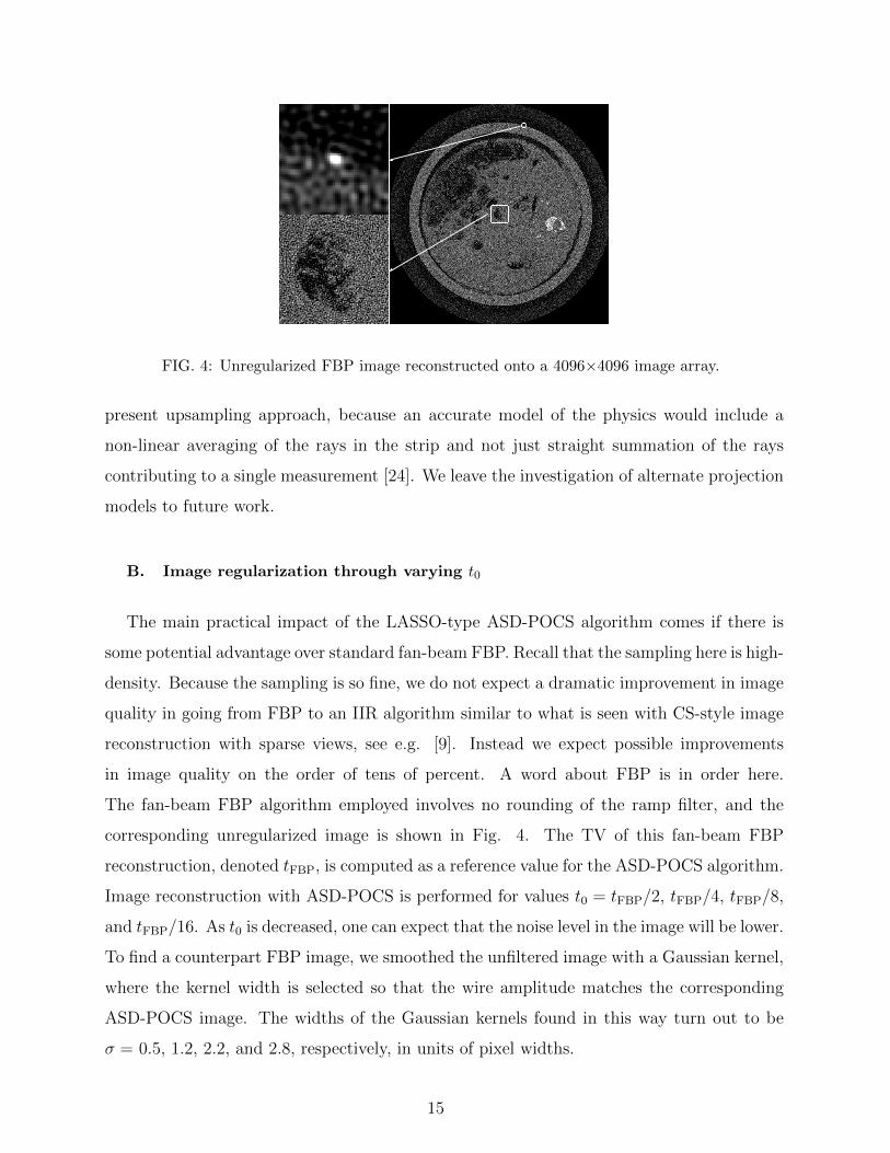
FIG. 4: Unregularized FBP image reconstructed onto a 4096×4096 image array.

present upsampling approach, because an accurate model of the physics would include a

non-linear averaging of the rays in the strip and not just straight summation of the rays

contributing to a single measurement [24]. We leave the investigation of alternate projection

models to future work.

B. Image regularization through varying t0

The main practical impact of the LASSO-type ASD-POCS algorithm comes if there is

some potential advantage over standard fan-beam FBP. Recall that the sampling here is high-

density. Because the sampling is so fine, we do not expect a dramatic improvement in image

quality in going from FBP to an IIR algorithm similar to what is seen with CS-style image

reconstruction with sparse views, see e.g. [9]. Instead we expect possible improvements

in image quality on the order of tens of percent. A word about FBP is in order here.

The fan-beam FBP algorithm employed involves no rounding of the ramp filter, and the

corresponding unregularized image is shown in Fig. 4. The TV of this fan-beam FBP

reconstruction, denoted tFBP, is computed as a reference value for the ASD-POCS algorithm.

Image reconstruction with ASD-POCS is performed for values t0 = tFBP/2, tFBP/4, tFBP/8,

and tFBP/16. As t0 is decreased, one can expect that the noise level in the image will be lower.

To find a counterpart FBP image, we smoothed the unfiltered image with a Gaussian kernel,

where the kernel width is selected so that the wire amplitude matches the corresponding

ASD-POCS image. The widths of the Gaussian kernels found in this way turn out to be

σ = 0.5, 1.2, 2.2, and 2.8, respectively, in units of pixel widths.

15

FIG. 5: Top: FBP image convolved with a Gaussian of width σ = 0.5. Bottom: ASD-POCS

reconstruction for t0 = tFBP/2. For each image the gray scale is [0, 0.06] mm−1 accept for the top,

left ROI containing the cross-section of the wire, which is displayed in a window of [0, 0.1] mm−1.

In Figs. 5 and 6, we show comparisons between the ASD-POCS images with the cor-

responding regularized FBP image for the least and greatest, respectively, amount of regu-

larization. Additionally, for more quantitative comparison, we show a series of ASD-POCS

profiles through the wire in Fig. 7 and the corresponding FBP profiles in Fig. 8.

We discuss the possible advantage of IIR with the LASSO-type ASD-POCS algorithm.

We point out again and it is clear from the images that potential advantages will be small

as we are trying to squeeze out more information from a very finely sampled system. Nev-

ertheless, there appears to be some advantage. Comparing Figs. 4 and 5, one can see that

the level of FBP regularization is negligible as both FBP images appear very similar. The

corresponding ASD-POCS image has some visible advantage, as the noise level is lower; this

is most easily seen in the lower left ROIs in the dark regions of the images. For all the image

16

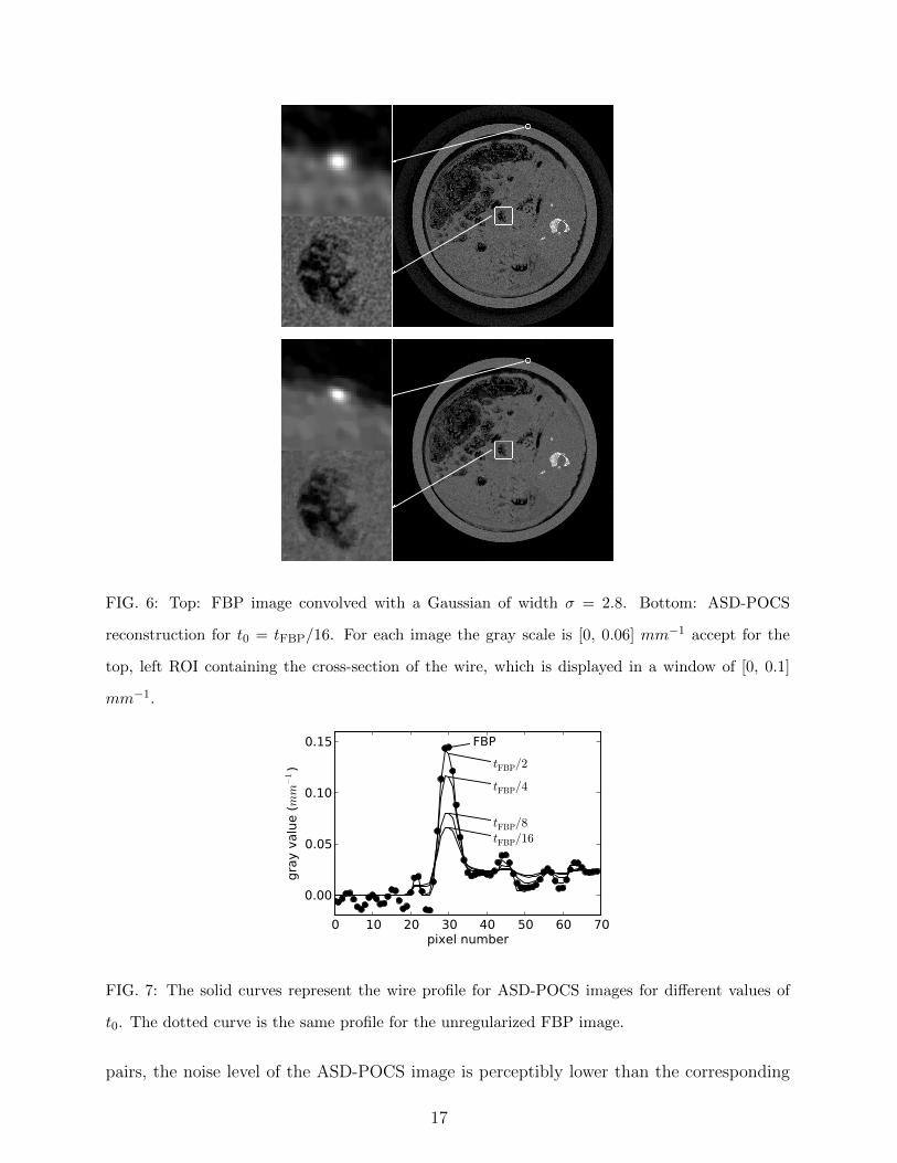
FIG. 6: Top: FBP image convolved with a Gaussian of width σ = 2.8. Bottom: ASD-POCS

reconstruction for t0 = tFBP/16. For each image the gray scale is [0, 0.06] mm−1 accept for the

top, left ROI containing the cross-section of the wire, which is displayed in a window of [0, 0.1]

mm−1.

0 10 20 30 40 50 60 70pixel number

0.00

0.05

0.10

0.15

gra

y v

alu

e (mm

�1 ) FBP

tFBP/2

tFBP/4

tFBP/8

tFBP/16

FIG. 7: The solid curves represent the wire profile for ASD-POCS images for different values of

t0. The dotted curve is the same profile for the unregularized FBP image.

pairs, the noise level of the ASD-POCS image is perceptibly lower than the corresponding

17

0 10 20 30 40 50 60 70pixel number

0.00

0.05

0.10

0.15

gra

y v

alu

e (mm

�1 ) FBP�=0.5�=1.2�=2.2�=2.8

FIG. 8: The solid curves represent the wire profile for FBP images smoothed by a Gaussian of

various widths. The dotted curve is the same profile for the unregularized FBP image.

FBP image. This can be seen quantitatively by computing the mean and standard deviation

of pixel values in a 200×200 square just above and to the right of the bone, where the sub-

ject’s gray value is uniform. The resulting values are displayed in a bar chart shown in Fig.

9. The profile plots in Figs. 7 and 8 illustrate another possible advantage to the ASD-POCS

algorithm. For ASD-POCS the wire profiles maintain their width as image TV is decreased,

while the Gaussian smoothed FBP profiles show spreading with increasing regularization.

This trend in the wire profile is also apparent in the 2D image of Fig. 6. In all the ASD-

POCS images the smallest ROI containing the wire cross-section still has some perceptible

graininess. This graininess can be effectively removed by further upsampling the data and

reconstructing onto an 8192×8192 image array. We found, however, that the resulting gain

in image quality is minimal for our purpose.

V. CONCLUSION

We have developed a CS-style image reconstruction algorithm for finely sampled projec-

tion data obtained with a low intensity X-ray beam. The main goals of the IIR algorithm

are to provide control over the image regularity and to image small objects of width compa-

rable to the detector bin. The technical points to achieve these goals are: (1) an upsampling

scheme for the projection data which takes advantage of the asymmetry in data sampling,

namely, that recognizes that the bin-direction of the data is sampled more finely than the

angular direction; and (2) conversion of the constrained, TV-minimization problem to a

18

raw FBP tFBP/2 tFBP/4 tFBP/8 tFBP/160.00

0.01

0.02

0.03

0.04

gra

y v

alu

e (mm

�1 ) FBPASD-POCS

FIG. 9: Mean and standard deviation over a 200×200 pixel region, where the subject is uniform.

The first column shows values for the unregularized FBP image of Fig. 4. The subsequent columns

are labeled by the t0 value used in the ASD-POCS reconstruction. The corresponding regularized

FBP result is obtained by Gaussian smoothing where the kernel width is selected by matching

the amplitude of the wire in the ASD-POCS image, as explained in the text. In each case the

ASD-POCS yields a standard deviation lower than that of the FBP image with equivalent contrast

of the wire object.

LASSO formulation for the purpose of deriving an alternate ASD-POCS algorithm which

efficiently solves the corresponding optimization problem to a high degree of accuracy. The

resulting algorithm appears to achieve the above mentioned goals.

Anecdotally, there have been complaints from radiologists that IIR images yield unreal-

istic looking images, which has been blamed on the different noise patterns from IIR and

FBP algorithms. We speculate that the real issue is that IIR algorithms implemented on

commercial scanners reduce the image resolution to gain in noise reduction in a way that is

difficult to control. Objects of size on the order of the detector bin are highly distorted in

standard IIR implementations. The presented ASD-POCS algorithm allows for more control

over this trade-off. We point out that the upsampling idea can be used with in conjunction

with any IIR algorithm – a subject for future investigation. Another direction which the

current work can be extended is the inclusion of more physics of the imaging process in the

LASSO optimization problem; for example, a data error term could be designed to more

closely match the noise model of this CT system.

Addressing now the main practical issue of dose reduction while maintaining image qual-

ity, we have developed an IIR algorithm for the extreme where IIR should have the least

19

impact – namely, fine sampling in the projection angle. Fixing the overall dose, but decreas-

ing the number of views should result in equal or better image quality for ASD-POCS as it

is originally designed for sparse-view sampling. Thus, there is a potential not only to reduce

dose, but to eliminate the need for expensive flying focal-spot technology on the X-ray source

[25]. This point, however, is presently speculation as it requires a more in-depth study on

data sets with similar exposure and different numbers of projections, and there may be an

additional practical issue from blurring if the X-ray source moves at a constant rotation rate

with fewer sampling intervals.

Acknowledgments

This work was supported in part by NIH R01 grants CA120540 and EB000225. The

contents of this article are solely the responsibility of the authors and do not necessarily

represent the official views of the National Institutes of Health.

[1] C. H. McCollough, A. N. Primak, N. Braun, J. Kofler, L. Yu, and J. Christner, Radiol. Clin.

N. Am. 47, 27 (2009).

[2] H. Erdogan and J. A. Fessler, Phys. Med. Biol 44, 2835 (1999).

[3] J. Qi and R. M. Leahy, Phys. Med. Biol. 51, R541 (2006).

[4] X. Pan, E. Y. Sidky, and M. Vannier, Inv. Prob. 25, 123009 (2009).

[5] M. Li, H. Yang, and H. Kudo, Phy. Med. Biol. 47, 2599 (2002).

[6] E. Y. Sidky, C.-M. Kao, and X. Pan, J. X-ray Sci. Tech. 14, 119 (2006).

[7] G. H. Chen, J. Tang, and S. Leng, Med. Phys. 35, 660 (2008).

[8] J. Song, Q. H. Liu, G. A. Johnson, and C. T. Badea, Med. Phys. 34, 4476 (2007).

[9] E. Y. Sidky and X. Pan, Phys. Med. Biol. 53, 4777 (2008).

[10] E. Y. Sidky, X. Pan, I. S. Reiser, R. M. Nishikawa, R. H. Moore, and D. B. Kopans, Med.

Phys. 36, 4920 (2009).

[11] E. Y. Sidky, M. A. Anastasio, and X. Pan, Opt. Express 18, 10404 (2010).

[12] X. Jia, Y. Lou, R. Li, W. Y. Song, and S. B. Jiang, Med. Phys. 37, 1757 (2010).

[13] K. Choi, J. Wang, L. Zhu, T.-S. Suh, S. Boyd, and L. Xing, Med. Phys. 37, 5113 (2010).

20

[14] F. Bergner, T. Berkus, M. Oelhafen, P. Kunz, T. Pan, R. Grimmer, L. Ritschl, and M. Kachel-

riess, Med. Phys. 37, 5044 (2010).

[15] E. J. Candes, J. Romberg, and T. Tao, IEEE Trans. Inf. Theory 52, 489 (2006).

[16] E. J. Candes, J. K. Romberg, and T. Tao, Comm. Pure Appl. Math. 59, 1207 (2006).

[17] E. J. Candes and M. B. Wakin, IEEE Signal Process. Mag. 25, 21 (2008).

[18] J. Bian, J. H. Siewerdsen, X. Han, E. Y. Sidky, J. L. Prince, C. A. Pelizzari, and X. Pan,

Phys. Med. Biol 55, 6575 (2010).

[19] T. Flohr, K. Stierstorfer, R. Raupach, S. Ulzheimer, and H. Bruder, RoFo: Fortschritte auf

dem Gebiete der Rontgenstrahlen und der Nuklearmedizin 176, 1803 (2004).

[20] M. Kachelriess, M. Knaup, C. Penssel, and W. A. Kalender, IEEE Trans. Nucl. Sci. 53, 1238

(2006).

[21] W. Zbijewski and F. J. Beekman, Phys. Med. Biol 49, 145 (2004).

[22] M. A. T. Figueiredo, R. D. Nowak, and S. J. Wright, IEEE J. Sel. Top. Sig. Proc. 4, 586

(2007).

[23] F. Xu and K. Mueller, IEEE Trans. Nucl. Sci. 53, 1238 (2006).

[24] Y. Zou, E. Y. Sidky, and X. Pan, Phys. Med. Biol 49, 2365 (2004).

[25] D. Xia, J. Bian, X. Han, E. Y. Sidky, and X. Pan, in IEEE Medical Imaging Conference Record

(Orlando, FL, 2009), pp. 3458–3462.

21