1294 IEEE TRANSACTIONS ON NEURAL NETWORKS, VOL. 18, NO. 5, SEPTEMBER 2007

Localized Generalization Error Model and ItsApplication to Architecture Selection for

Radial Basis Function Neural NetworkDaniel S. Yeung, Fellow, IEEE, Wing W. Y. Ng, Member, IEEE, Defeng Wang, Eric C. C. Tsang, Member, IEEE,

and Xi-Zhao Wang, Senior Member, IEEE

Abstract—The generalization error bounds found by currenterror models using the number of effective parameters of a clas-sifier and the number of training samples are usually very loose.These bounds are intended for the entire input space. However,support vector machine (SVM), radial basis function neuralnetwork (RBFNN), and multilayer perceptron neural network(MLPNN) are local learning machines for solving problems andtreat unseen samples near the training samples to be more im-portant. In this paper, we propose a localized generalization errormodel which bounds from above the generalization error within aneighborhood of the training samples using stochastic sensitivitymeasure. It is then used to develop an architecture selection tech-nique for a classifier with maximal coverage of unseen samplesby specifying a generalization error threshold. Experiments using17 University of California at Irvine (UCI) data sets show that, incomparison with cross validation (CV), sequential learning, andtwo other ad hoc methods, our technique consistently yields thebest testing classification accuracy with fewer hidden neurons andless training time.

Index Terms—Localized generalization error, network architec-ture selection, radial basis function neural network (RBFNN), sen-sitivity measure.

I. INTRODUCTION

FOR a pattern classification problem, one builds a classifierto approximate or mimic the unknown input–output

mapping function , where is the set of parameters selectedfrom a domain . In this paper, the mean square error (MSE)is used to measure the difference between and . TheMSE is widely applied in training real-value output classi-fiers like neural networks, which classify a given sample bythresholding the real-value classifier output. The behavior of a

Manuscript received September 14, 2005; revised March 2, 2006 and De-cember 24, 2006; accepted December 26, 2006. This paper was supported inpart by the Hong Kong Research Grant Council under Project B-Q571, in partby the Hong Kong Polytechnic University Department of Computing PersonalResearch Account, and in part by the Hong Kong Polytechnic University Inter-faculty under Research Grant GYD87.

D. S. Yeung and W. W. Y. Ng are with the Media and Life Science (MiLeS),Department of Computer Science and Technology, Shenzhen Graduate School,Harbin Institute of Technology, Shenzhen 518055, China and with the De-partment of Computing, Hong Kong Polytechnic University, Kowloon, HongKong(e-mail: csdaniel@comp.polyu.edu.hk; wingng@ieee.org).

D. Wang and E. C. C. Tsang are with the Department of Computing, HongKong Polytechnic University, Kowloon, Hong Kong.

X.-Z. Wang is with the Machine Learning Center, Faculty of Mathematicsand Computer Science, Hebei University, Baoding 071002, China.

Color versions of one or more of the figures in this paper are available onlineat http://ieeexplore.ieee.org.

Digital Object Identifier 10.1109/TNN.2007.894058

classifier trained by minimizing an MSE and the one trainedby minimizing a classification error (0–1 loss function) aredifferent. When two classifiers both yield the same, very smallpercentage of training classification error, the one which yieldsa larger training MSE would produce indecisive outputs whichare more deviated from the target outputs; so a small changein the inputs may change the classification results [20]. Thisis not desirable and it indicates that the training classificationerror is not a good benchmark for the generalization capabilityof a classifier. Therefore, selecting a classifier using trainingclassification error or its bound may not be appropriate.

The classification error for the entire input space is defined as

(1)

where denotes the input vector of a sample in the entire inputspace , and denotes the true unknown probability densityfunction of the input .

Given a training data set containing traininginput–output pairs, , a classifiercould be constructed by minimizing the empirical riskover , where

(2)

The ultimate goal of solving a pattern classification problemis to find which is able to correctly classify future unseensamples [6], [10], [17]. The generalization error is de-fined as

(3)

Since both target outputs and distributions of the unseen sam-ples are unknown, it is impossible to compute the directly.There are two major approaches to estimate the , namely,analytical model and cross validation (CV).

In general, analytical models could not distinguish trainedclassifiers having the same number of effective parameters butwith different values of parameters. Thus, they yield loose errorbounds [5]. Akaike information criterion (AIC) [1] only makesuse of the number of effective parameters and the number oftraining samples. Network information criterion (NIC) [15]is an extension of AIC for application in regularized neuralnetworks. It defines a classifier complexity by the trace of the

1045-9227/$25.00 © 2007 IEEE

YEUNG et al.: LOCALIZED GENERALIZATION ERROR MODEL AND ITS APPLICATION TO ARCHITECTURE SELECTION FOR RBFNN 1295

second-order local derivatives of the network outputs withrespect to connection weights. Unfortunately, current analyticalmodels are only good for linear classifiers due to the singularityproblem in their models [16]. A major problem with thesemodels is the difficulty in estimating the number of effectiveparameters of the classifier and this could be solved by using theVapnik–Chervonenkis (VC)-dimensions [17]. However, onlyloose bounds of VC-dimensions could be found for nonlinearclassifiers and this puts a severe limitation on the applicabilityof analytical models to nonlinear classifiers, except for thesupport vector machine (SVM) [3], [4], [5].

Although CV uses true target outputs for unseen samples, itis time consuming for large data sets and, for -fold CV andchoices of classifier parameters, classifiers must be trained.CV methods estimate the expected generalization error insteadof its bound. Thus, they cannot guarantee the classifier finallyconstructed to have good generalization capability [5].

Many classifiers, e.g., SVM, multilayer perceptron neuralnetworks (MLPNNs), and radial basis function neural net-works (RBFNNs), are local learning machines. RBFNN, byits nature, learns the classification locally and every hiddenneuron captures the local information of a particular region inthe input space defined by the center and width of its Gaussianactivation function [11]. A training sample located far awayfrom a hidden neuron’s center does not affect the learning ofthis hidden neuron [8]. MLPNN learns the decision boundariesfor the classification problem in the input space using thelocation of the training samples. However, as pointed out in[2], the MLPNN output responses to unseen samples far awayfrom the training samples are likely to be unreliable, so theyproposed a learning algorithm which deactivates any MLPNNresponse to unseen samples much different from the trainingsamples. This observation is further supported by the fact that,in many interesting industrial applications, such as aircraft de-tection in synthetic aperture radar (SAR) images, character andfingerprint recognitions [9], etc., the most significant unseensamples are expected to be similar to the training samples.

On the other hand, RBFNN is one of the most widely ap-plied neural networks for pattern classification, with its perfor-mance primarily determined by its architecture selection. Ref-erence [6] summarizes several training algorithms for RBFNN.For instance, a two-stage learning algorithm may be a quick wayto train an RBFNN. The first, unsupervised stage is to select thecenter positions and widths for the RBF using self-organizingmap or -means clustering. The second, supervised stage com-putes the connection weights using least mean square method orpseudoinverse technique. Some proposed that all training sam-ples may be selected as centers [6], [22]. In [18], a reformu-lated RBFNN was proposed which was trained by using a gra-dient-descent method for its parameters. In [26], the selectionof centers is based on the separability of the data sets. The ex-perimental results in [18] and [26] indicate that the choice ofthe number of hidden neurons indeed affect the generalizationcapability of the RBFNNs and an increase in the number ofhidden neurons does not necessarily lead to a decrease in testingerror. In [23] and [24], the optimal architecture was found by se-quentially adding more hidden neurons to a small RBFNN and,in [25], genetic algorithm was used to search for the optimal

number of hidden neurons, center position, and width, simulta-neously. Thus, the selection of the number of hidden neuronsaffects the selection of RBFNN architecture and ad hoc choicesor sequential search are the frequently used methods.

In this paper, we propose a localized generalization errormodel using the stochastic sensitivity measure (ST-SM),which bounds from above the generalization error for unseensamples within a predefined neighborhood of the trainingsamples. In addition, an architecture selection method basedon the is proposed to find the maximal coverage classifierwith its bounded by a preselected threshold. RBFNN willbe used to demonstrate the use of the and the architectureselection method.

We introduce the localized generalization error model andits corresponding architecture selection method in Sections IIand III, respectively. In Section IV, experimental results of thearchitecture selection will be presented. We conclude this paperin Section V.

II. LOCALIZED GENERALIZATION ERROR MODEL

Two major concepts of , the -neighborhood and sto-chastic sensitivity measure, are introduced in Sections II-A andII-C, respectively. The derivation of the localized generalizationerror model is given in Section II-B and its characteristics arediscussed in Section II-D. Section II-E discusses the method tocompare two classifiers using the localized generalization errormodel.

A. Q-Neighborhood and Q-Union

For every sample , one finds a set of samples whichfulfills , where denotes thenumber of input features, ,and is a given real number. In pattern classification problem,one usually does not have any knowledge about the distributionof the true input space. Therefore, without any prior knowledge,every unseen sample has the same chance to appear; so, maybe considered as input perturbations which are random variableshaving zero mean uniform distributions

(4)Then, defines a -neighborhood of the training

sample . Let be the union of all and call it the-union. All samples in , except , are considered as

unseen samples (i.e., contains no training point otherthan ).

For , the following relationshipholds:

(5)

One should note that the shape of the -neighborhood ischosen to be a hypercube for ease of computation, but it couldalso be a hypersphere or other shapes. Moreover, in the local-ized generalization error model, the unseen samples could beselected from a distribution other than a uniform one. Only the

1296 IEEE TRANSACTIONS ON NEURAL NETWORKS, VOL. 18, NO. 5, SEPTEMBER 2007

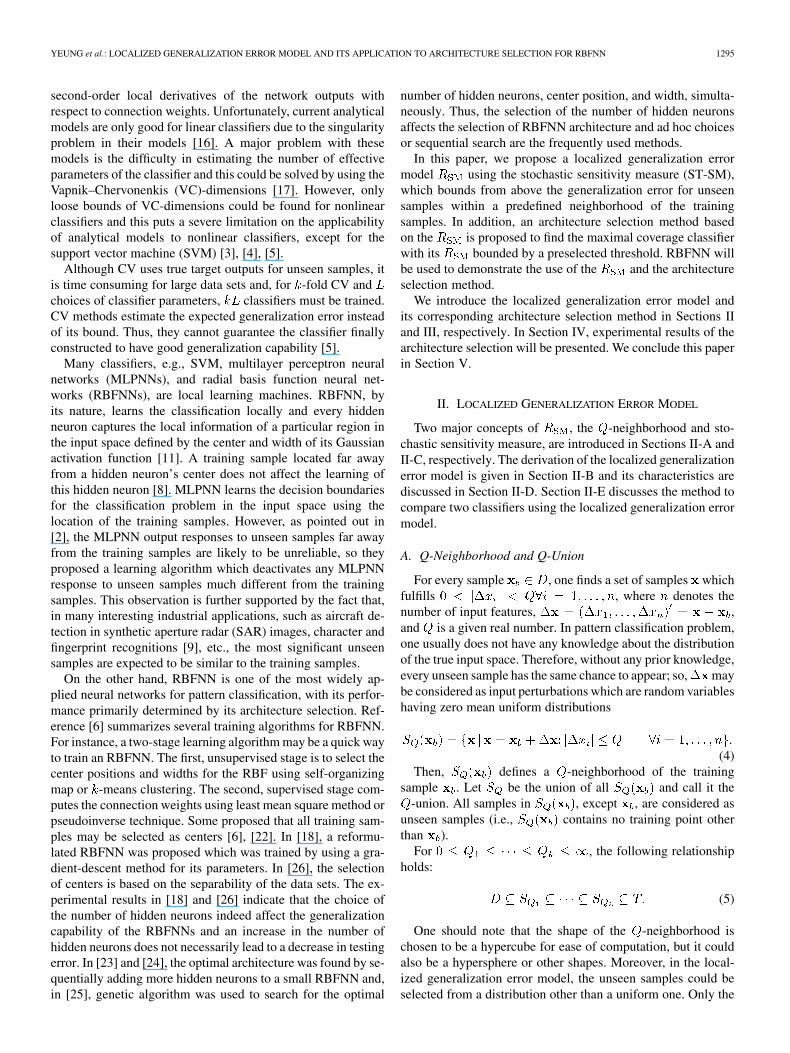
Fig. 1. Illustration of Q-union (S ) with 20 training samples. The Xs aretraining samples and any point in the shaded area is an unseen sample.

derivation of the ST-SM needs to be modified and the rest of thepaper will remain the same.

B. Derivation of the Localized Generalization Error Bound

Instead of finding a bound for the generalization error forunseen samples in the entire input space , we find abound on , which is the error for unseen samples within

only, i.e., the shaded area in Fig. 1. We ignore the gener-alization error for unseen samples which are located far awayfrom training samples [ in (6)]. Note that decreaseswhen increases

(6)Let

then

and , and be the differencebetween the maximum and minimum values of the targetoutputs, the maximum possible value of the MSE, and thenumber of training samples, respectively. In this paper, weassume the range of the desired output, i.e., the range of , to

be either known or assigned to a preselected value. Moreover,is computable because the range of the network outputs will

be known after the classifier is trained. In general, one expectsthat the error of unseen samples will be larger than the trainingerror, so we assume that the average of errors of unseensamples in will be larger than the training error of .By the Hoeffding’s inequality [7], the average of the squareerrors of samples with the same population mean converges tothe true mean with the following rate of convergence. With aprobability of , we have (7), as shown at the bottom ofthe page.

Both and are constants for a given training data set whenan upper bound of the classifier output values is preselected. The

is an upper bound for the MSE of the trained classifier forunseen samples within the -union. This bound is better thanthose regression error bounds (based on AIC and VC-dimen-sion) which are defined by using only the number of effectiveparameters and training samples while ignoring statistical char-acteristics of training data set such as their mean and variance.Moreover, those error bounds usually grow quickly with the in-crease of the number of effective parameters, e.g., number ofhidden neurons in RBFNN and VC-dimension, while thegrows much slower.

The term will be discussed in Section II-C. Fur-ther discussion on the characteristics of the will be givenin Section II-D.

C. Stochastic Sensitivity Measure for RBFNN

The output perturbation measures the network outputdifference between the training sample and the unseensample in its -neighborhood . Thus,the ST-SM measures the expectation of the squares of network

(7)

YEUNG et al.: LOCALIZED GENERALIZATION ERROR MODEL AND ITS APPLICATION TO ARCHITECTURE SELECTION FOR RBFNN 1297

output perturbations between training samples in andunseen samples in .

The sensitivity measure (SM) of a neural network [12]–[14]gives a quantified data on the change of network outputs with re-spect to change of network inputs. Intuitively, it measures howsensitive the network output is to the input change. In [14], everyinput or weight is allowed to have its own mean and variance,and the input and weight perturbations are allowed to be arbi-trary. Hence, the perturbed samples ( in Section II-A) can beconsidered as unseen samples around the training samples .An analytical formula of the ST-SM for a Gaussian activationfunction RBFNN was developed in [12], which is independentof the number of training samples. We assume the inputs areindependent and not identically distributed and weight pertur-bations are not considered in this paper; so, every input featurehas its own expectation and variance . The input per-turbation of the th input feature is a random variable having auniform distribution with zero mean and a variance . Thecenters and widths of the hidden neurons are constant and theconnection weights are fixed beforehand. An RBFNN could bedescribed as

(8)

where , , and denote the number of hidden neurons,the center, and width of the th RBFNN hidden neuron, respec-tively, and denotes the connection weight between the thhidden neuron and its corresponding output neuron. Let

, ,

,

denotes the probability density function of the input per-turbations and , is the number of input fea-tures and denotes the th input feature of the th center ofthe hidden RBF neuron . For uniformlydistributed input perturbations, we have

. Theoretically, we do not restrict the distribution of theinput perturbations as long as the variance of the input perturba-tion is finite. However, uniform distribution is assumedhere because without any prior knowledge on the distribution ofunseen samples around the training samples, we assume that allof them have an equal chance of occurrence.

By the law of large numbers, when the number of input fea-tures is not too low, would have a log-normal distribution;so, the RBFNN ST-SM is given by

(9)

D. Characteristics of the

From (7), one may notice that the consists of three majorcomponents: training error , ST-SM , andthe constants. The constants and are preselected when theconfidence of the bound and the training data set arefixed. Moreover, the constant in could be preselected whenthe classifier type is selected by fixing the maximum classifieroutput bound. is generally very small for large ; so, they willnot affect the result of comparisons of the generalization capa-bility between classifiers. In contrast, if the classifier could notgeneralize the training samples, one may not expect the classi-fier to have good generalization capability to future unseen sam-ples. Thus, the training error is one of the key components of the

. Furthermore, the ST-SM term measures the output fluc-tuations of the classifier. A classifier having high output fluctu-ations yields high ST-SM because its output varies dramaticallywhen the input value changes. Due to the classifier bias/variancedilemma, a classifier yielding a good generalization capabilityshould minimize both terms or achieves a good balance betweenthe two [19].

An interesting question is: Can be an effective mecha-nism for studying a classifier’s bias/variance dilemma?

1) Limiting Cases of : Obviously, when, and . For

, the relationshipholds. We further extend this relationship to

the limiting case of with

with (10)

This relationship shows that the limiting case ofwith bounds from above the . For

(11)

1298 IEEE TRANSACTIONS ON NEURAL NETWORKS, VOL. 18, NO. 5, SEPTEMBER 2007

Moreover, for the limiting case of boundsfrom above. When vanishes, and

we have

(12)

2) for Other Classifiers: The as well as thecould be defined for any classifier trained with MSE. Examplesinclude feedforward neural networks like MLPNN, SVM, andrecurrent neural networks such as Hopfield networks. Thefor other types of classifier could be defined by rederiving theST-SM term for the particular type of classifier concerned.

3) Independence of Training Method: The is deter-mined with no regard to the training methods being used. Onlythe parameters of the finally trained classifier are used in themodel. Hence, the model could also be used to comparedifferent training methods in terms of the generalization capa-bility of the classifiers being built.

4) Time Complexity: The ST-SM has a time complexity of. The computational complexities of both the ST-SM

and the are low and they do not depend on the numberof training samples . However, similar to all other archi-tecture selection methods, requires a trained classifier andthe time for architecture selections is dominated by the classi-fier training time. Therefore, the proposed architecture selectionmethod may not have a large advantage in terms of speed whenbeing compared with other architecture selection methods, ex-cept the two CV-based methods.

5) Limitations of the Localized Generalization Error Model:The major limitation of the localized generalization error modelis that it requires a function (i.e., ) for the derivation of theST-SM. Classifiers such as rule-based system and decisiontree may not be able to make use of this concept. It will be achallenging task to find way to determine the for theseclassifiers.

Another limitation of the present localized generalizationerror model is due to the assumption that unseen samples areuniformly distributed. This assumption is reasonable whenthere is no a priori knowledge on the true distribution of theinput space, and hence, every sample may have the same prob-ability of occurrence. One would need to rederive a newwhen a different distribution of the input space is assumed.We also remark that even though the distribution of the unseensamples is known, their true target outputs are still unknown,and hence, it will be difficult to judge how good the bound is.On the other hand, if both input and -union distributions arethe same, the localized generalization error model is expectedto be a good estimation for the generalization error for theunseen samples, but this needs further investigation.

6) and Regularization: From (9), one may notice thatthe connection weight magnitude ( in the ) is directly pro-portional to the ST-SM, and thus, the . This provides a the-oretical justification that, by controlling the magnitude of theconnection weights between hidden and output layers, one couldreduce the generalization error which is essential to the regular-ization of neural network learning [6].

7) Predicting Unseen Samples Outside the Q-Union: In prac-tice, some unseen samples may be located outside the -union.This may be due to the fact that the value is too small, andthus, the -union covers only very few unseen samples. How-ever, expanding the value will lead to a larger , because

more dissimilar unseen samples are included in the -union,and a classifier with very large upper bound may not bemeaningful. Furthermore, the bounds from above the MSEof the unseen samples and the MSE is an average of the errors.Thus, the bound may still work well even though some ofthe unseen samples are located outside the -union. This is sup-ported by the experimental results presented in a Section IV-B.When splitting the training and testing data sets, naturally someunseen testing samples may fall outside the -union. However,our experiments show that the generalization capability of theRBFNNs selected by using the is still the best in terms oftesting accuracy when compared with other methods.

On the other hand, if there is a large portion of unseen sampleslocated outside the -union, i.e., dissimilar to the training sam-ples, one may consider revising the training data set to includemore such samples and retrain the classifier. As mentioned be-fore, classifiers may not be expected to classify unseen samplesthat are totally different from the training set. We will describean experiment for this scenario in Section IV-C.

E. Comparing Two Classifiers Using the

One way to compare two classifiers is to fix thevalue and compare the difference between their values. Theother way is to fix the value and compare the of thetwo classifiers.

Assume there are two classifiers, and . There exists afor yielding and a for yielding

. If , then has a better generaliza-tion capability because covers more unseen samples but stillhas the same generalization error upper bound. In other words,the architecture selection could be done by searching the func-tional space and seek with the largest producing

. This is an important property of and wewill make use of it to find the optimal classifier with the largestcoverage in Section III.

On the other hand, one could compare the two classifiers,and , based on their computed using the samevalue. The classifier with lower is expected to have abetter generalization capability.

All other comparison methods by not fixing either ormay not be meaningful.

III. ARCHITECTURE SELECTION USING WITH

SELECTED MC SG

The selection of the number of hidden neurons in the RBFNNis usually done by sequential learning [8], [23], [24], [29] or byad hoc choice. The sequential learning technique only makes useof the training error to determine the number of hidden neurons,without any reference to the generalization capability. More-over, [8] and [29] assume that the classifier does not have priorknowledge about the number of training samples while [23] and[24] do. For ease of comparison with other architecture selectionmethod, we assume that the number of training samples in ourexperiments is known to the classifier. In this section, we pro-pose a new technique based on to find the optimal numberof hidden neurons which makes use of the generalization capa-bility of the RBFNN.

YEUNG et al.: LOCALIZED GENERALIZATION ERROR MODEL AND ITS APPLICATION TO ARCHITECTURE SELECTION FOR RBFNN 1299

For any given threshold on generalization error bound, the localized generalization error model allows us to

find the best classifier by maximizing , assuming that theMSE of all samples within the -union is smaller than . Onecan formulate the architecture selection problem as a maximalcoverage classification problem with selected generalizationerror bound (MC SG), i.e.,

subject to (13)

In the RBFNN training algorithm presented in Section III-B,once the number of hidden neurons is fixed, the center posi-tions and widths could be estimated by any automatic clusteringalgorithm such as -means clustering, self-organizing map, orhierarchical clustering; so we only need to concentrate on theproblem of determining the number of hidden neurons. Thismeans that and because it is notreasonable to have the number of hidden neurons higher thanthe number of training samples.

Problem (13) is a 2-D optimization problem. The first dimen-sion is the number of hidden neurons and the second di-mension is the for a fixed . For every fixed and , wecan determine . These two parameters, and , are in-dependent. Furthermore, by substituting (9) into the (7), withprobability , we have the for RBFNN as follows:

(14)

Let . For every , let the that satisfiesbe , where is a constant real number

existing because the second-order derivative of(14) is positive. We could solve (14) as follows:

(15)

Equation (15) could be solved by the quadratic equation andtwo solutions will be found for . For and beingusually a very small constant when the number of samples islarge, there will be one positive and one negative real solutionfor because, in (15), the coefficients for the terms andare positive, but the constant term is negative. This means thatthere will be two real and two imaginary solutions for and let

be the only positive real solution among the four. Note thatis defined to be the width of the -neighborhood and as such

it must be a nonnegative real number

else(16)

For RBFNN architecture selection, (13) is equivalent to

(17)

A. Parameters for MC SG

In (7), the difference between the maximum and minimumvalues of target outputs and the number of training samples

are fixed for a given training data set, and the maximumpossible value of the MSE and the confidence level of thebound, namely, and , could also be selected before any clas-sifier training.

In a -class classification problem, one may selectwhere and .

if the sample belongs to the th class, and one minimizes theMSE of all the RBFNN outputs simultaneously. All the

, and are vectors, and thus, the sum of s of allthe RBFNN outputs are minimized in the MC SG. One maynotice that the minimization of the sum of s of all the out-puts is equivalent to the minimization of the average of them.However, the average of s may provide a better interpreta-tion and its range is not affected by the value .

The determination of the constant is made according tothe classifier’s output schemes for classification. For instance,if class outputs are different by one, then may be selected as0.25 because a sample is misclassified if the square of its devi-ation from the target output is larger than 0.25. From (16), onemay notice that the smaller is, the larger number of hiddenneurons will be selected by the MC SG because the value ofthose RBFNNs will be zero if its training error is larger than the

value and training error decreases as the of number of hiddenneurons increases. On the other hand, if the value is selectedto be larger than 0.25, the effect to the architecture selection willbe insignificant. Experimental results show that those RBFNNsyielding training error larger than 0.25 will not yield good gen-eralization capability, i.e., poor testing accuracies.

B. RBFNN Architecture Selection Algorithm for MC SG

The solution of (17) is realized using the following selectionalgorithm. The SG is independent of any training algo-rithm of the RBFNN. However, one of the fast RBFNN trainingmethods is employed in this paper for all of the experiments[11]. Steps 2) and 3) are the unsupervised learning to find thecenters and widths of the RBFs in the hidden neurons and Step4) finds the least-square solution of the connection weights bymaking use of the linear relationship, shown in (8), between thehidden neuron outputs and RBFNN outputs. Other training al-gorithms could be adopted in Steps 2)–4) in the following archi-tecture selection algorithm.

The architecture selection algorithm of the MC SG is asfollows.

1) Start with ( denotes the number of hiddenneurons).

2) Perform -means clustering algorithm to find the centersfor the hidden neurons.

3) For each of the RBF hidden neurons, select its widthvalue to be the distance between the center of itself and theone of the nearest hidden neuron.

4) Compute the connection weights using a pseudoinversemethod.

5) Compute the -value for the current RBFNN using (16).6) If the stopping criterion is not fulfilled, and

go to Step 2).The stopping criterion could be selected as “ is equal to

the number of training samples” and this will allow the MC SGto search for all possible number of hidden neurons. However,

1300 IEEE TRANSACTIONS ON NEURAL NETWORKS, VOL. 18, NO. 5, SEPTEMBER 2007

it is computationally prohibited for large data set and we willdiscuss heuristic stopping criterion in Section III-C. Moreover,constructive approach is employed here because it is more ef-ficient to start the search with one hidden neuron, and add onehidden neuron for each iteration.

C. Heuristic Method to Reduce the Computational Time forMC SG

Same as the other methods, is generally not differ-entiable with respect to (not a smooth function). One musttry out all possible values in order to find the optimal so-lution. Our experimental results show that drops tozero when the classifier becomes too complex, i.e., is toolarge, and heuristically, an early stop could be made to reducethe number of classifier trainings when approaches zero. Inour experiments, we stop the search when the values dropbelow a threshold. In fact, does not increase significantly afterit drops below 10% of the maximum value of being found,and thus, it is used as the threshold to speed up the MC SG.

IV. EXPERIMENTS ON 17 BENCHMARKING UCI DATA SETS

The experimental setup is explained in Section IV-A and wepresent and discuss the experimental results in Section IV-B.Section IV-C shows the special case when the training samplesare drawn with bias.

A. Experimental Setup

In this section, we compare the MC SG with well-known ar-chitecture selection methods [5], [6]:CV, sequential learning,and two ad hoc methods. Steps 2)–4) of the architecture selec-tion algorithm presented in Section III-B are used to train theRBFNNs for all architecture selection methods. Every data setis divided into two parts, training and testing, and each consistsof 50% of the samples. This is repeated ten times to generate tenindependent runs for each data set. Table II shows the averageclassification accuracies on the testing sets for these ten runs.The testing data set is treated as future unseen samples. All in-puts are scaled to to eliminate the effect of large values.Seventeen real-world data sets from the UCI machine learningrepository Table I are used. A wide range of data sets is selectedfrom image classification, medical informatics, network secu-rity, and financial applications. The “DAPRA99 DoS” consistsof normal and denial of service (DoS) types of samples fromthe 10% training data set of DAPRA99 data set [21]. The mul-tiple feature data set consists of large number of features whileDAPRA99 DoS, waveform, mushroom, and optical digit datasets consist of large number of samples. In addition, small datasets, e.g., iris, wine, and thyroid gland, and medium data sets areselected to demonstrate that the proposed method MC SG canbe applied to any variation of classification problems in numbersof samples, features, and classes. Moreover, in the experiments,a sample is considered to be incorrect if its error is larger than0.5 (a squared error of 0.25), and therefore, we will useas the threshold value for the in MC SG.

As suggested in [5], fivefolds (5-CV) and tenfolds (10-CV)CVs are used in our experiments. In a -fold CV, the trainingdata set is divided into disjoint partitions and one of them

TABLE ISEVENTEEN BENCHMARKING DATA SETS

is used as the validation set. classifiers are trained using dif-ferent partitions and the average of these validation errorsis used as the CV error. The number of hidden neurons whichyields the lowest CV error will be selected. The “sequen_MSE”and “sequen_01” methods are to add hidden neurons until, re-spectively, the training MSE and the classification erroris minimized. The ad hoc method denoted by “ ” uses everytraining sample as a center of RBFNN hidden neurons. Theother ad hoc method “SQRT ” selects the number of hiddenneurons to be equal to the square root of the number of trainingsamples.

B. Experimental Results and Analysis

Experimental results in Tables II and III show that theMC SG performs best among the methods consistently interms of highest average classification accuracy for unseensamples, smaller average number of hidden neurons, and fastin training times without regarding to the numbers of trainingsamples, features, and classes of the data sets. However, wenote that the differences in terms of average testing accuraciesare not very big, therefore, one-tailed McNemar tests [27],[28] were performed to examine the statistical significance ofthe improvements made by the MC SG. Table IV shows thatthe RBFNNs selected by MC SG are statistically significantlybetter than those RBFNNs selected by other methods at 0.05level of significance (i.e., McNemar test value larger than 2.71).Furthermore, the statistical significances shown in Table IVindicate that the proposed method outperforms other methodmore significantly when the number of training samples islarge. It is also interesting to observe that from Tables II and IV,none of the other six methods performs the second best consis-tently in all of the experiments while the MC SG consistentlyperforms best for all 17 data sets.

Table III shows that the CV method is very time consuming,and it requires 5 to 10 000 times longer to find the best RBFNN.The reason that less time is required by the MC SG than the twosequential learning methods is due to the early stopping of the

YEUNG et al.: LOCALIZED GENERALIZATION ERROR MODEL AND ITS APPLICATION TO ARCHITECTURE SELECTION FOR RBFNN 1301

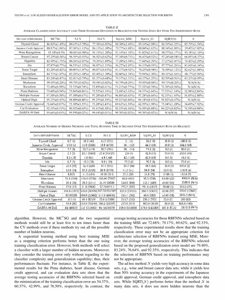
TABLE IIAVERAGE CLASSIFICATION ACCURACY (AND THEIR STANDARD DEVIATION IN BRACKETS) FOR TESTING DATA SET OVER TEN INDEPENDENT RUNS

TABLE IIIAVERAGE NUMBER OF HIDDEN NEURONS AND TOTAL RUNNING TIME IN SECONDS OVER TEN INDEPENDENT RUNS (IN BRACKET)

algorithm. However, the MC SG and the two sequentialmethods would still be at least five to ten times faster thanthe CV methods even if these methods try out all the possiblenumber of hidden neurons.

A sequential learning method using best training MSEas a stopping criterion performs better than the one usingtraining classification error. However, both methods will selecta classifier with a larger number of hidden neurons. Moreover,they consider the training error only without regarding to theclassifier complexity and generalization capability; thus, theirperformances fluctuate. For instance, in Table II, the experi-mental results for the Pima diabetes, heart disease, Germancredit approval, and car evaluation data sets show that theaverage testing accuracies of the RBFNNs selected based onthe minimization of the training classification error are 54.37%,60.37%, 42.99%, and 76.50%, respectively. In contrast, the

average testing accuracies for those RBFNNs selected based onthe training MSE are 72.68%, 79.17%, 69.62%, and 92.33%,respectively. These experimental results show that the trainingclassification error may not be an appropriate criterion forarchitecture selection of RBFNNs trained using MSE. More-over, the average testing accuracies of the RBFNNs selectedbased on the proposed generalization error model are 79.40%,83.24%, 76.64%, and 92.35%, respectively. This indicates thatthe selection of RBFNN based on training performance maynot be appropriate.

The ad hoc method yields very high accuracy in some datasets, e.g., wine and breast cancer data sets, while it yields lessthan 50% testing accuracy in the experiments of the Japanesecredit approval, German credit approval, and ionosphere datasets. While SQRT performs better than the method inmany data sets, it does use more hidden neurons than the

1302 IEEE TRANSACTIONS ON NEURAL NETWORKS, VOL. 18, NO. 5, SEPTEMBER 2007

TABLE IVMCNEMAR TEST STATISTICS BETWEEN MC SG AND OTHER METHODS FOR TESTING DATA SET OVER TEN INDEPENDENT RUNS

TABLE VEXPERIMENTAL RESULTS FOR THE BIASED TRAINING DATA SET FOR THE UCI THYROID GLAND DATA SET

MC SG for virtually the same level of classification accuracy.For example, from the breast cancer data set, the MC SG usesnine times less hidden neurons than the SQRT . Both ad hocmethods are fast in training time because they employ prese-lected number of hidden neurons; however, this number is usu-ally too large. In addition, for data sets consisting of extremelylarge number of training samples, both ad hoc methods may se-lect an unreasonable number of hidden neurons. For example,the method selects 247 010 hidden neurons for the DAPRA99DoS data set which is infeasible for training.

One may notice that the testing accuracies of some data sets,e.g., waveform, ionosphere, and German credit approval, are notvery high. However, our aim of presenting these experimentalresults here is not to demonstrate the superiority of our methodfor all data sets. Our aim is to present an overall comparisonof the performance of the RBFNNs constructed by our pro-posed method and that of other popular methods using the sametraining and testing data sets.

C. Experiments on a Biased Data Set

With a random splitting of training and testing data sets, the-union of the training samples usually covers most of the

testing samples with a small value, i.e., the testing samplesare similar to training samples. This would also be the case inreal-world applications of pattern classifier that unseen samplesmay not be very dissimilar to the training ones.

In some cases when the training data set is sampled poorly, theclassifier being trained using this data set would perform poorlyfor future unseen samples. However, the interesting question is:

Will the MC SG still be working well in such cases? We per-formed a biased sampling using the thyroid gland data set be-cause this data set consists of fewer features and thus is easierfor visualization. Training samples are selected if its value infeature 1 is less than 0.57 such that the training and testing sam-ples are approximately splitting in half and their distributionsare shown in Fig. 3. Then, we swap the training and testing datasets to obtain the second run of this experiment. These processesare repeated for the other four features to obtain ten trainingand testing data set pairs. The results shown in Table V are theaverage over these ten trials. Fig. 2 shows the distributions oftraining and testing samples in a random, unbiased splitting, andthe shaded area in Figs. 2 and 3 is the coverage of the -union.From Figs. 2 and 3, one may notice that most of the testing sam-ples are covered by the -union in random splitting while a largeportion of testing samples are located outside the -union in thebiased splitting. From Table V, one may notice that the accu-racies of the classifiers selected by all methods are lower than60%; however the MC SG still outperforms other architectureselection methods. This indicates that the minimization of thelocal generalization error helps minimizing the generalizationerror even for unseen samples that deviated from the trainingsamples a lot.

One may notice that the training error in such a biased trainingdata set is misleading. Thus, CV methods which depend on re-sampling from the training samples may not provide good esti-mation of the generalization error. The two sequential learningmethods depend totally on the training error and they performworse than the MC SG; however, interestingly, they performbetter than the CV methods. This may be due to the fact thatCV methods make use of only a portion of the biased training

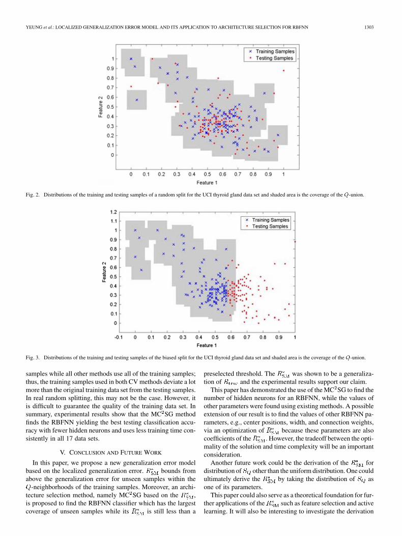
YEUNG et al.: LOCALIZED GENERALIZATION ERROR MODEL AND ITS APPLICATION TO ARCHITECTURE SELECTION FOR RBFNN 1303

Fig. 2. Distributions of the training and testing samples of a random split for the UCI thyroid gland data set and shaded area is the coverage of the Q-union.

Fig. 3. Distributions of the training and testing samples of the biased split for the UCI thyroid gland data set and shaded area is the coverage of the Q-union.

samples while all other methods use all of the training samples;thus, the training samples used in both CV methods deviate a lotmore than the original training data set from the testing samples.In real random splitting, this may not be the case. However, itis difficult to guarantee the quality of the training data set. Insummary, experimental results show that the MC SG methodfinds the RBFNN yielding the best testing classification accu-racy with fewer hidden neurons and uses less training time con-sistently in all 17 data sets.

V. CONCLUSION AND FUTURE WORK

In this paper, we propose a new generalization error modelbased on the localized generalization error. bounds fromabove the generalization error for unseen samples within the

-neighborhoods of the training samples. Moreover, an archi-tecture selection method, namely MC SG based on the ,is proposed to find the RBFNN classifier which has the largestcoverage of unseen samples while its is still less than a

preselected threshold. The was shown to be a generaliza-tion of and the experimental results support our claim.

This paper has demonstrated the use of the MC SG to find thenumber of hidden neurons for an RBFNN, while the values ofother parameters were found using existing methods. A possibleextension of our result is to find the values of other RBFNN pa-rameters, e.g., center positions, width, and connection weights,via an optimization of because these parameters are alsocoefficients of the . However, the tradeoff between the opti-mality of the solution and time complexity will be an importantconsideration.

Another future work could be the derivation of the fordistribution of other than the uniform distribution. One couldultimately derive the by taking the distribution of asone of its parameters.

This paper could also serve as a theoretical foundation for fur-ther applications of the such as feature selection and activelearning. It will also be interesting to investigate the derivation

1304 IEEE TRANSACTIONS ON NEURAL NETWORKS, VOL. 18, NO. 5, SEPTEMBER 2007

of the ST-SM for other classifiers or using objective functionsother than MSE for classifier training.

ACKNOWLEDGMENT

The authors would like to thank the six reviewers who pro-vided very helpful comments.

REFERENCES

[1] H. Akaike, “A Bayesian analysis of the minimum AIC procedure,” Ann.Inst. Statist. Math., pp. 9–14, 1978.

[2] D. Chakraborty and N. R. Pal, “A novel training scheme for multi-layered perceptrons to realize proper generalization and incrementallearning,” IEEE Trans. Neural Netw., vol. 14, no. 1, pp. 1–14, Jan. 2003.

[3] V. Cherkassky and F. Mulier, Learning From Data. New York:Wiley, 1998.

[4] V. Cherkassky, X. Shao, F. M. Mulier, and V. N. Vapnik, “Model com-plexity control for regression using VC generalization bounds,” IEEETrans. Neural Netw., vol. 10, no. 5, pp. 1075–1089, Sep. 1999.

[5] T. Hastie, R. Tibshirani, and J. Friedman, The Element of StatisticalLearning. New York: Springer-Verlag, 2001.

[6] S. Haykin, Neural Networks. Englewood Cliffs, NJ: Prentice-Hall,1998.

[7] W. Hoeffding, “Probability inequalities for sums of bounded randomvariables,” J. Amer. Statist. Assoc., vol. 58, pp. 13–30, 1963.

[8] G.-B. Huang, P. Saratchandran, and N. Sundararajan, “A generalizedgrowing and pruning RBF (GGAP-RBF) neural network for functionapproximation,” IEEE Trans. Neural Netw., vol. 16, no. 1, pp. 57–67,Jan. 2005.

[9] L. C. Jain and V. R. Venuri, Eds., Industrial Applications of NeuralNetworks. Boca Raton, FL: CRC Press, 1999.

[10] T. M. Mitchell, Machine Learning. New York: McGraw-Hill, 1997.[11] J. Moody and C. J. Darken, “Fast learning in networks of locally-tuned

processing units,” Neural Comput., pp. 281–294, 1989.[12] W. W. Y. Ng and D. S. Yeung, “Selection of weight quantisation accu-

racy for radial basis function neural network using stochastic sensitivitymeasure,” Inst. Electr. Eng. Electron. Lett., pp. 787–789, 2003.

[13] W. W. Y. Ng, D. S. Yeung, X.-Z. Wang, and I. Cloete, “A study ofthe difference between partial derivative and stochastic neural networksensitivity analysis for applications in supervised pattern classifica-tion problems,” in Proc. Int. Conf. Mach. Learn. Cybern., 2004, pp.4283–4288.

[14] W. W. Y. Ng, D. S. Yeung, and I. Cloete, “Quantitative study on ef-fect of center selection to RBFNN classification performance,” in IEEEProc. Int. Conf. Syst., Man, Cybern., 2004, pp. 3692–3697.

[15] H. Park, N. Murata, and S.-I. Amari, “Improving generalization per-formance of natural gradient learning using optimized regularizationby NIC,” Neural Comput., pp. 355–382, 2004.

[16] S. Watanabe, “Algebraic analysis for nonidentifiable learning ma-chines,” Neural Comput., vol. 13, pp. 899–933, 2001.

[17] V. Vapnik, Statistical Learning Theory. New York: Wiley, 1998.[18] N. B. Karayiannis and M. M. Randolph-Gips, “On the construction and

training of reformulated radial basis function neural networks,” IEEETrans. Neural Netw., vol. 14, no. 4, pp. 835–846, Jul. 2003.

[19] S. Geman and E. Bienenstock, “Neural networks and the bias/variancedilemma,” Neural Comput., vol. 4, pp. 1–58, 1992.

[20] M. Anthony and P. L. Bartlett, Neural Network Learning: TheoreticalFoundations. Cambridge, U.K.: Cambridge Univ. Press, 1999.

[21] W. W. Y. Ng, R. K. C. Chang, and D. S. Yeung, “Dimensionalityreduction for denial of service detection problems using RBFNNoutput sensitivity,” in Proc. Int. Conf. Mach. Learn. Cybern., 2003,pp. 1293–1298.

[22] Y.-J. Oyang, S.-C. Hwang, Y.-Y. Ou, C.-Y. Chen, and Z.-W. Chen,“Data classification with radial basis function networks based on anovel kernel density estimation algorithm,” IEEE Trans. Neural Netw.,vol. 16, no. 1, pp. 225–236, Jan. 2005.

[23] W. Kaminski and P. Strumillo, “Kernel orthonormalization in radialbasis function neural networks,” IEEE Trans. Neural Netw., vol. 8, no.5, pp. 1177–1183, Sep. 1997.

[24] J. B. Gomm and D. L. Yu, “Selecting radial basis function networkcenters with recursive orthogonal least squares training,” IEEE Trans.Neural Netw., vol. 11, no. 2, pp. 306–314, Mar. 2000.

[25] H. Leung, N. Dubash, and N. Xie, “Detection of small objects in clutterusing a GA-RBF neural network,” IEEE Trans. Aerosp. Electron. Syst.,vol. 38, no. 1, pp. 98–118, Jan. 2002.

[26] K. Z. Mao, “RBF neural network center selection based on fisher ratioclass separability measure,” IEEE Trans. Neural Netw., vol. 13, no. 5,pp. 1211–1217, Sep. 2002.

[27] S. L. Salzberg, “On comparing classifiers: A critique of current re-search and methods,” Data Mining Knowl. Disc., pp. 317–327, 1997.

[28] D. J. Sheskin, Handbook of Parametric and Nonparametric StatisticalProcedures. London, U.K.: Chapman & Hall, 2004.

[29] N.-Y. Liang, G.-B. Huang, P. Saratchandran, and N. Sundararajan, “Afast and accurate online sequential learning algorithm for feedforwardnetworks,” IEEE Trans. Neural Netw., vol. 17, no. 6, pp. 1411–1423,Nov. 2006.

Daniel S. Yeung (M’89–SM’99–F’04) received thePh.D. degree in applied mathematics from CaseWestern Reserve University, Cleveland, OH, in 1974.

In the past, he has worked as an Assistant Professorof Mathematics and Computer Science at RochesterInstitute of Technology, as a Research Scientist inthe General Electric Corporate Research Center, andas a System Integration Engineer at TRW. He wasthe chairman of the Department of Computing, TheHong Kong Polytechnic University, Hong Kong. Heleads a group of researchers in Hong Kong and China

who are actively engaging in research works on computational intelligence anddata mining. His current research interests include neural network sensitivityanalysis, data mining, Chinese computing, and fuzzy systems.

Dr. Yeung was the President of IEEE Hong Kong Computer Chapter, anAssociate Editor for both the IEEE TRANSACTIONS ON NEURAL NETWORKS

and the IEEE TRANSACTIONS ON SYSTEMS, MAN, AND CYBERNETICS—PART

B: CYBERNETICS. He has been elected as President Elect for the IEEE Sys-tems, Man, and Cybernetics Society. He served as a General Co-Chair of the2002–2007 International Conference on Machine Learning and Cyberneticsheld annually in China, and a Keynote Speaker for the same Conference.His IEEE Fellow citation makes reference to his “contribution in the area ofsensitivity analysis of neural networks and fuzzy expert systems.”

Wing W. Y. Ng (S’01–M’06) received the B.Sc. de-gree in information technology and the Ph.D. degreein computer science from the Hong Kong PolytechnicUniversity, Kowloon, Hong Kong, in 2001 and 2006,respectively.

In 2006, he joined the Media and Life Science(MiLeS) Computing Laboratory, Department ofComputer Science and Technology, Shenzhen Grad-uate School, Harbin Institute of Technology, China,where he is currently an Assistant Professor. Hismajor research interests include media computing,

localized generalization error model, feature selection, active learning, andneural network sensitivity analysis.

Dr. Ng is the Co-Chair of Technical Committee on Computational Intelli-gence, IEEE Systems, Man and Cybernetics Society. He was also the Founderand Chairman of Hong Kong Polytechnic University Student Branch Chapter,IEEE Systems, Man and Cybernetics Society. He served as the Conference Sec-retary of the 2002–2007 International Conference on Machine Learning and Cy-bernetics held annually in China.

Defeng Wang (S’03) received the B.Eng. degreein computer application from Jilin University,Changchun, China, in 2000, the M.Eng. degreein computer application from Xidian University,Shaanxi, China, in 2003, and the Ph.D. degree fromThe Hong Kong Polytechnic University, Kowloon,Hong Kong, in 2006.

His recent research is focused on kernel methods,large margin learning, and medical image analysis.

YEUNG et al.: LOCALIZED GENERALIZATION ERROR MODEL AND ITS APPLICATION TO ARCHITECTURE SELECTION FOR RBFNN 1305

Eric C. C. Tsang (M’04) received the B.Sc. degreein computer studies from the City University of HongKong, Hong Kong, in 1990 and the Ph.D. degree incomputing from the Hong Kong Polytechnic Univer-sity, Kowloon, Hong Kong, in 1996.

He is an Assistant Professor at the Department ofComputing, the Hong Kong Polytechnic University.His main research interests are in the area of fuzzyexpert systems, fuzzy neural networks, machinelearning, genetic algorithm, rough sets, fuzzy roughsets, fuzzy support vector machine, and multiple

classifier system.

Xi-Zhao Wang (M’98–SM’02) received the B.Sc.and M.Sc. degrees in mathematics from HebeiUniversity, Baoding, China, in 1983 and 1992, re-spectively, and the Ph.D. degree in computer sciencefrom Harbin Institute of Technology, Harbin, China,in 1998.

From 1983 to 1998, he worked as a Lecturer,an Associate Professor, and a Full Professor atthe Department of Mathematics, Hebei University.From 1998 to 2001, he worked as a ResearchFellow at the Department of Computing, Hong Kong

Polytechnic University, Kowloon, Hong Kong. Since 2001, he has been theDean and Professor of the Faculty of Mathematics and Computer Science,Hebei University. His main research interests include inductive learning withfuzzy representation, fuzzy measures and integrals, neurofuzzy systems andgenetic algorithms, feature extraction, multiclassifier fusion, and applicationsof machine learning. He has published over 60 international journal papers,completed over 20 funded research projects, and supervised over 30 doctorateor Masters degrees.

Prof. Xi-Zhao Wang is an Associate Editor of IEEE TRANSACTIONS ON

SYSTEMS, MAN, AND CYBERNETICS—PART B: CYBERNETICS, an AssociateEditor of International Journal of Information Sciences, Chair of IEEE Sys-tems, Man, and Cybernetics Baoding Chapter; Chair of IEEE Systems, Man,and Cybernetics Technical Committee on Computational Intelligence, and anExecutive Member of Chinese Association of Artificial Intelligence. He is theGeneral Co-Chair of the 2002, 2003, 2004, 2005, 2006, and 2007 InternationalConference on Machine Learning and Cybernetics, cosponsored by IEEESystems, Man, and Cybernetics Society.