CIplus Band 5/2016

Stacked Generalization of Surrogate Models - A Practical Approach Thomas Bartz-Beielstein

Stacked Generalization of Surrogate ModelsA Practical Approach

Thomas Bartz-BeielsteinTH Köln

Computer Science and Engineering Sciencethomas.bartz-beielstein@th-koeln.de

http://www.spotseven.de

May 29, 2016

Abstract

This report presents a practical approach to stacked generalization in surrogate modelbased optimization. It exemplifies the integration of stacking methods into the surrogate modelbuilding process. First, a brief overview of the current state in surrogate model based opti-mization is presented. Stacked generalization is introduced as a promising ensemble surrogatemodeling approach. Then two examples (the first is based on a real world application andthe second on a set of artificial test functions) are presented. These examples clearly illustratetwo properties of stacked generalization: (i) combining information from two poor performingmodels can result in a good performing model and (ii) even if the ensemble contains a goodperforming model, combining its information with information from poor performing modelsresults in a relatively small performance decrease only.

1 Introduction

The selection of an adequate meta model is crucial in model based optimization (MBO). Modelbased optimization plays a prominent role in todays modeling, simulation, and optimizationprocesses. It is one of the most efficient technique for expensive and time demanding real-world optimization problems. Especially in the engineering domain, MBO is an importanttechnique. This popularity is caused by recent advances in computer science, statistics, andengineering, in combination with progress in high-performance computing. A combinationof theses advanced tools enable the treatment of problems considered unsolvable only a fewdecades ago. We will consider MBO in the context of global optimization.

Global optimization (GO) can be categorized on different criteria, e.g., the properties ofthe problems (continuous versus combinatorial, linear versus non-linear, convex versus non-convex, etc.). In many real world situations, GO problems are difficult, because nearly nostructural information (e.g., number of local extrema) is available. These kind of GO problemsbelong to the class of black-box functions, i.e., the analytic form is unknown. Note, the classof black-box function contains also functions that are easy to solve, e.g., convex functions. Theoptimization problem is given by

minimize: f(~x) subject to ~xl ≤ ~x ≤ ~xu,

where f : Rn → R is referred to as the objective function and ~xl and ~xu denote the lowerand upper bounds of the search space (region of interest), respectively. This setting arises in

1

many real-world systems, i.e., when the explicit form of the objective function f is not readilyavailable or e.g., user has no access to the source code of a simulator.

The term GO will be used for algorithms that are trying to find and explore global optimalsolutions with complex, multimodal objective functions [36]. We will use an algorithmic view,i.e., we will consider the properties of algorithms.

First, we will describe stochastic (random) search algorithms and show how surrogatemodel based optimization can be classified in the context of GO. Therefore we introduce thefollowing taxonomy.

1. Deterministic

2. Random Search

(a) Instance based.(b) Model based optimization (MBO).

i. Distribution based.ii. Surrogate Model Based Optimization (SBO).

A. Single surrogate based.B. Multi-fidelity based.C. Evolutionary surrogate based.D. Ensemble surrogate based.

Then, we will try to answer the question of selecting an adequate surrogate model in the con-text of SBO.

Tis report is structured as follows: First, SBO is presented in the context of stochastic searchalgorithms (Section 2). Section 3 presents some general considerations about using multiplesurrogate models. The sequential parameter optimization (SPO), which uses SBO, is introduced inSection 4. Stacked generalization is one important modeling technique in SPO. An industrialapplication is used in Section 5 for introducing the key features of the stacked generalizationapproach. To gain further insight, a second study, which uses artificial test functions, is pre-sented in Section 6. This report concludes with a short summary and an outlook in Section 7.

2 Stochastic Search Algorithms

To motivate the importance of model selection in MBO, we will describe the related GO algo-rithms first. Stochastic search algorithms perform an iterative search. They use a stochasticprocedure to generate the next iterate. The next iterate can be a candidate solution to the GO ora probabilistic model, where solutions can be drawn from. Stochastic search algorithms do notdepend on any structural information of the objective function such as gradient informationor convexity. Hence, they are robust and easy to implement. Stochastic search algorithms canfurther be categorized as instance-based or model-based algorithms [51]

Instance-based algorithms use a single solution, ~x, or population, P (t), of candidate solu-tions. The construction of new candidates depends explicitly on previously generated solu-tions. Prominent examples are simulated annealing or evolutionary algorithms.

Model-based optimization algorithms generate a population of new candidate solutionsP ′(t) by sampling from a model. In statistics, the terms model and distribution are used synony-mously. Therefore, we will use the term surrogate model, when we are referring to an explicitmodel. The model (or distribution) reflects structural properties of the underlying true func-tion, say f . Adapting the model (or the distribution), the search is directed into regions withimproved solutions. One of the key ideas in MBO can be formulated as follows: replace ex-pensive, high fidelity, fine grained function evaluations, f(~x), with evaluations, f(~x), of anadequate surrogate model, say M . Surrogate models also known as the cheap model, the re-sponse surface, the meta model, the approximation, or the coarse grained model.

2

2.1 Distribution-based Approaches

Distribution-based optimization algorithms maintain a distribution as a metamodel. A se-quence of iterates, i.e., probability distributions, {p(t)} is generated. The iterates should havethe property, that

p(t)→ p∗ as t→∞,where p∗ is the limiting distribution, which assigns most of its probability mass to the set ofoptimal solutions. Note, distribution-based optimization algorithms propagate a probabilitydistribution from one iteration to the next, whereas instance-based algorithms propagate can-didate solutions ~x.

Estimation of distribution algorithms (EDA) are very popular in the field of evolutionary algo-rithms (EA). Variation operators such as mutation and recombination are replaced by a distri-bution based procedure. A probability distribution, which is estimated from promising can-didate solutions from the current population, is used to generate new population. [27] reviewdifferent ways for using probabilistic models. [18] discuss advantages and outline many of thedifferent types of EDAs. [19] present recent approaches and a unified view.

Although distribution-based approaches play an important role in GO, they will not bediscussed further in this report. We will concentrate on surrogate model based approaches,which have their origin in statistical design and analysis of experiments, especially in responsesurface methodology [12] [31].

2.2 Surrogate Model-based Approaches

In general, the term surrogate is used, when the outcome of a process cannot be directly mea-sured. A surrogate tries to imitate the behavior of the real model as closely as possible whilebeing computationally cheaper to evaluate. Simple surrogate models can be constructed us-ing a data-driven approach. They can be refined by integrating additional points or domainknowledge, e.g., constraints.

A wide range of surrogates were developed in the last decades. This results in complexdesign decisions. Following the discussion in [47], surrogate design decisions are necessary forthe selection of (i) metamodels, (ii) designs, and (iii) model fitting methods.

Metamodels Typical metamodels are (a) classical regression models such as polynomial re-gression or response surface methodology [12] [31] (b) support vector machines} (SVM)[46] (c) neural networks [52] (d) radial basis functions [35], or (e) Gaussian process (GP)models, also known as design and analysis of computer experiments or Kriging [42] [7],[1], [26], [41]. [10] presents a comprehensive introduction to SBO.

Designs A broad variety of designs are available, e.g., classical experimental designs such asfactorial, fractional factorial, central composite, or A-, D-optimal (alphabetically) designs.Alternatively, space filling designs, such as simple grids, Latin hypercube designs, or-thogonal or uniform designs can be used. In addition, hybrid designs, random or humanselection, and sequential design methods are available.

Model Fit Model fitting can be based on several criteria, e.g., weighted least squares regres-sion or maximum likelihood estimation. Special fitting techniques exist for specific mod-eling approacches, e.g., backpropagation for neural networks.

2.3 SBO Applications

Simulation-based design of complex engineering problems, e.g., computational fluid dynamics(CFD) and finite element modeling (FEM) methods are the most popular application areas forSBO. To generate exact solutions, the corresponding solvers require a large number of expen-sive computer simulations. Generally, there are two SBO variants: (i) metamodel based meth-ods, which use one or several different metamodels and (ii) multi-fidelity approximation meth-ods, which uses several instances with different parameterizations of the same metamodel.

3

Helicopter rotor design optimization [4], aerodynamic shape design [13], multi-objectiveoptimal design of a liquid rocket injector [38], and aerospace design [11] are only a few exam-ples of SBO in industry.

Multi-fidelity approximation is used in [20], who use several simulation models with dif-ferent grid sizes in FEM and in [44], who optimize a sheet metal forming process.

2.4 Surrogate-assisted Evolutionary Algorithms

Surrogate-assisted EA use a cheap surrogate model to replace evaluations of expensive ob-jective function. Several variants of surrogate-assisted EAs were developed in the last years,e.g., a combination of a genetic algorithm and neural networks for aerodynamic design opti-mization [16], an approximate model of the fitness landscape using Kriging interpolation toaccelerate the convergence of EAs [39], an Evolution strategy (ES) with neural network basedfitness evaluations [24], or a surrogate-assisted EA framework with online learning [50]. Asurvey of surrogate-assisted EA approaches is presented in [23]. SBO approaches for evolutionstrategies are described in [9].

3 Multiple Models and Model Selection

Instead of using one surrogate model only, several models Mi, i = 1, 2, . . . , p, generated andevaluated in parallel can be used. Each model Mi : X → y uses the same candidate solutions,X , from the population P and the same results, y, from expensive function evaluations.

Multiple models can also be used to partition the search space. Here we can mention tree-based Gaussian processes, which use regression trees to partition the search space and fit localGP surrogates in each region [15]. A tree-based partitioning of an aerodynamic design space,which uses independent Kriging surfaces in each partition, is described in [33]. The combi-nation of an evolutionary model selection algorithm with expected improvement (EI) criterion,which selects the best performing surrogate model type at each iteration of the EI algorithmwas proposed by [8].

Ensembles of surrogate models gained popularity. An adaptive weighted average modelof the individual surrogates was presented in [49]. An approach which uses the best surro-gate model or a weighted average surrogate model instead was introduced in [14]. In theseapproaches, the models for the ensemble are chosen based on their performance. Usually, theweights are adaptive and inversely proportional to the local modeling errors.

The simplest model selection process is a refinement method: the same (initial) model willbe refined during the optimization. This method requires a selection criteria for samplingnew points, so-called infill points. The balance between exploration, i.e., improving the modelquality (related to the model, global), and exploitation, i.e., improving the optimization anddetermining the optimum (related to the objective function, local) plays a central role in thisstrategy. Expected improvement (EI) is a popular adaptive sampling method [30] [25].

The EI approach handles the initialization and refinement of a surrogate model, but notthe selection of the model itself. For example, the popular efficient global optimization (EGO)algorithm uses a Kriging model, because Kriging inherently determines the prediction variance(necessary for the EI criterion). But there is no proof that Kriging is the best choice. Alternativesurrogate models, e.g., neural networks, regression trees, support vector machines, or lassoand ridge regression may be better suited. However: An a priory selection of the best suitedsurrogate model is conceptually impossible in the framework treated in this report, because ofthe black-box setting.

Regarding the model choice, the user can decide whether to use (i) one single model, i.e.,one unique global model or (ii) multiple models, i.e., an ensemble of different, possibly local,models.

Now, we do not consider the selection of a new sample point (as done in EI). Instead, we

4

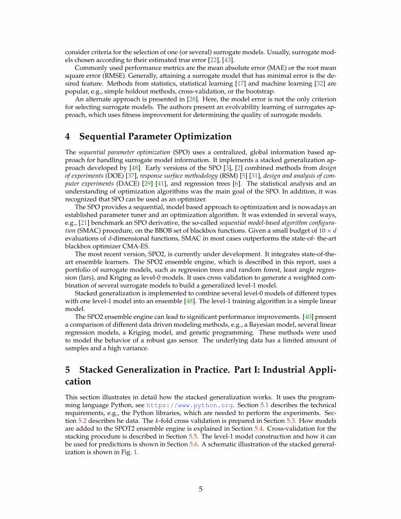
consider criteria for the selection of one (or several) surrogate models. Usually, surrogate mod-els chosen according to their estimated true error [22], [43].

Commonly used performance metrics are the mean absolute error (MAE) or the root meansquare error (RMSE). Generally, attaining a surrogate model that has minimal error is the de-sired feature. Methods from statistics, statistical learning [17] and machine learning [32] arepopular, e.g., simple holdout methods, cross-validation, or the bootstrap.

An alternate approach is presented in [28]. Here, the model error is not the only criterionfor selecting surrogate models. The authors present an evolvability learning of surrogates ap-proach, which uses fitness improvement for determining the quality of surrogate models.

4 Sequential Parameter Optimization

The sequential parameter optimization (SPO) uses a centralized, global information based ap-proach for handling surrogate model information. It implements a stacked generalization ap-proach developed by [48]. Early versions of the SPO [3], [2] combined methods from designof experiments (DOE) [37], response surface methodology (RSM) [5] [31], design and analysis of com-puter experiments (DACE) [29] [41], and regression trees [6]. The statistical analysis and anunderstanding of optimization algorithms was the main goal of the SPO. In addition, it wasrecognized that SPO can be used as an optimizer.

The SPO provides a sequential, model based approach to optimization and is nowadays anestablished parameter tuner and an optimization algorithm. It was extended in several ways,e.g., [21] benchmark an SPO derivative, the so-called sequential model-based algorithm configura-tion (SMAC) procedure, on the BBOB set of blackbox functions. Given a small budget of 10× devaluations of d-dimensional functions, SMAC in most cases outperforms the state-of- the-artblackbox optimizer CMA-ES.

The most recent version, SPO2, is currently under development. It integrates state-of-the-art ensemble learners. The SPO2 ensemble engine, which is described in this report, uses aportfolio of surrogate models, such as regression trees and random forest, least angle regres-sion (lars), and Kriging as level-0 models. It uses cross validation to generate a weighted com-bination of several surrogate models to build a generalized level-1 model.

Stacked generalization is implemented to combine several level-0 models of different typeswith one level-1 model into an ensemble [48]. The level-1 training algorithm is a simple linearmodel.

The SPO2 ensemble engine can lead to significant performance improvements. [40] presenta comparison of different data driven modeling methods, e.g., a Bayesian model, several linearregression models, a Kriging model, and genetic programming. These methods were usedto model the behavior of a robust gas sensor. The underlying data has a limited amount ofsamples and a high variance.

5 Stacked Generalization in Practice. Part I: Industrial Appli-cation

This section illustrates in detail how the stacked generalization works. It uses the program-ming language Python, see https://www.python.org. Section 5.1 describes the technicalrequirements, e.g., the Python libraries, which are needed to perform the experiments. Sec-tion 5.2 describes he data. The k-fold cross validation is prepared in Section 5.3. How modelsare added to the SPOT2 ensemble engine is explained in Section 5.4. Cross-validation for thestacking procedure is described in Section 5.5. The level-1 model construction and how it canbe used for predictions is shown in Section 5.6. A schematic illustration of the stacked general-ization is shown in Fig. 1.

5

Data

Training:{(Xi, yi)}i=1,...n{(Xi, yi)}i=1,...n

{yti}{yti}

A1A1 A2A2Val_Training:{(Xi, yi)}i=1,...q{(Xi, yi)}i=1,...q

Val_Test:{(Xi, yi)}i=q+1,...n{(Xi, yi)}i=q+1,...n

AV1AV1 AV

2AV2

Val_Test:{(Xi)}i=q+1,...n{(Xi)}i=q+1,...n

Val_Test:{(yi)}i=q+1,...n{(yi)}i=q+1,...nyAV

1yAV

1

yAV2

yAV2

A3A3 A(y,y)3A(y,y)3

ATr2ATr2ATr

1ATr1

yAT r1

yAT r1

yAT r2

yAT r2

yy

{Xti}{Xti}

Test:{(Xti, yti)}i=1,...,m{(Xti, yti)}i=1,...,m

Figure 1: Illustration of the data flow in stacked generalization. The data is split into a test andtraining set. The training data is used for CV, i.e., in each fold, a new training and validation dataset is generated. Here, we consider two algorithms, say A1 and A2, which are used to generatetwo level-0 models, AV

1 and AV2 . These models are used for predictions on the validation data set,

which result in predictions yAV1

and yAV2

. A level-1 algorithm, A3 is fitted to the data sets yAV1

,

yAV2

, and the yi’s from the validation data set. The resulting model, A(y,y)3 , is used for the final

predictions.

6

5.1 Technical Requirements

This section illustrates and demonstrates the key ingredients of the SPO2 ensemble engine. Itimplements ideas from [48] and is based on Python code from [34]. First, we have to

1. import libraries and

2. set the SPO2 parameters, i.e., the number of folds for the cross-validations.

import sysimport matplotlibimport matplotlib.pyplot as pltimport numpy as npimport pandas as pdimport statsmodels.formula.api as smimport mathfrom IPython.display import set_matplotlib_formatsfrom __future__ import divisionfrom sklearn.model_selection import KFoldfrom sklearn.ensemble import RandomForestRegressorfrom sklearn.linear_model import LinearRegressionfrom sklearn.metrics import mean_squared_errorfrom sklearn.metrics import r2_scorefrom pandas import read_csv

np.random.seed(0) # seed to shuffle the train setn_folds = 10

5.2 The Data

The complete data set is described in [40]. It consists of two separate data sets for two differentgas sensors: one training data set and one test data set. Here, we consider data from thesecond sensor. There are seven input values and one output value (y). The goal of this study isto predict the outcome y using the seven input measurements.

In [10]: dfTrain = read_csv('training.csv')dfTest = read_csv('testing.csv')XTrain = dfTrain.ix[:,0:7]yTrain = dfTrain.ix[:,7:9]yTrain1 = yTrain.ix[:,1]X = XTrain.as_matrix()y = yTrain1.as_matrix()XTest1 = dfTest.ix[:,0:7]yTest1 = dfTest.ix[:,7:9]yTest = yTest1.ix[:,1]XTest = XTest1.as_matrix()

5.3 CV Splits

The training data are split into folds. KFold() divides all the samples in k = nfolds groups ofsamples (called folds) of equal sizes (if possible). The prediction function is learned using k−1folds, and the fold left out is used for test.

In [11]: skf = KFold(n_folds);skf.get_n_splits(X, y);

7

5.4 Level-0 Models in the Ensemble

A linear regression model and a random forest regression model are included in this study.Additional models such as Lasso or Gaussian process models can be included very easily.

In [12]: models = [LinearRegression(), RandomForestRegressor()]

5.5 Cross-Validation

Let n denote the size of the training set (number of samples in the training set) and p thenumber of models. Summarizing, we will consider the following dimensions:

• n: size of the training set (samples)• k: number of folds for CV• p: number of models• m: size of the test data (samples)

We will use two matrices to store the CV results:

1. YCV is a (n× p)-matrix. It stores the results from the cross validation for each model. Thetraining set is partitioned into k folds (n_folds=k).

2. YBT is a (m× p)-matrix. It stores the aggregated results from the cross validation modelson the test data. For each fold, p separate models are build, which are used for predictionon the test data. The predicted values from the k folds are averaged for each model, whichresults in (m× p) different values.

In [13]: YCV = np.zeros((X.shape[0], len(models)))YBT = np.zeros((XTest.shape[0], len(models)))

for j, AV in enumerate(models):YBT_j = np.zeros((XTest.shape[0], skf.n_folds))for i, (train, val) in enumerate(list(skf.split(X,y))):

XValTraining = X[train,]yValTraining = y[train]XValTest = X[val]AV.fit(XValTraining, yValTraining)YCV[val, j] = AV.predict(XValTest)YBT_j[:, i] = AV.predict(XTest)

YBT[:,j] = YBT_j.mean(1)

5.6 The Level-1 Model

5.6.1 Model Building

The level-1 model is a function of the CV-values of each model to the known, training y-values.It provides an estimate of the influence of the single models. For example, if a linear level-1model is used, the coefficient βi represents the effect of the i-th model.

5.6.2 Model Prediction

The level-1 model is used for predictions on the YBT data, i.e., on the averaged predictions ofthe CV-models. It is constructed using the effects of the predicted values of the single models(determined by linear regression) on the true values of the training data. If a model predicts asimilar value as the true value during the CV, then it has a strong effect.

8

3 2 1 0 1 2 3

Measured

3

2

1

0

1

2

3

4

Pre

dic

ted

SPO2

L

R

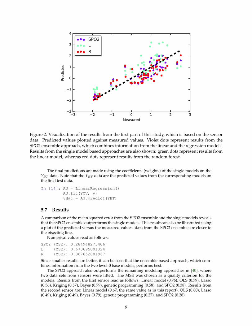
Figure 2: Visualization of the results from the first part of this study, which is based on the sensordata. Predicted values plotted against measured values. Violet dots represent results from theSPO2 ensemble approach, which combines information from the linear and the regression models.Results from the single model based approaches are also shown: green dots represent results fromthe linear model, whereas red dots represent results from the random forest.

The final predictions are made using the coefficients (weights) of the single models on theYBT data. Note that the YBT data are the predicted values from the corresponding models onthe final test data.

In [14]: A3 = LinearRegression()A3.fit(YCV, y)yHat = A3.predict(YBT)

5.7 Results

A comparison of the mean squared error from the SPO2 ensemble and the single models revealsthat the SPO2 ensemble outperforms the single models. This result can also be illustrated usinga plot of the predicted versus the measured values: data from the SPO2 ensemble are closer tothe bisecting line.

Numerical values read as follows:

SPO2 (MSE): 0.284948273406L (MSE): 0.673695001324R (MSE): 0.367652881967

Since smaller results are better, it can be seen that the ensemble-based approach, which com-bines information from the two level-0 base models, performs best.

The SPO2 approach also outperforms the remaining modeling approaches in [40], wheretwo data sets from sensors were fitted. The MSE was chosen as a quality criterion for themodels. Results from the first sensor read as follows: Linear model (0.76), OLS (0.79), Lasso(0.56), Kriging (0.57), Bayes (0.79), genetic programming (0.58), and SPO2 (0.38). Results fromthe second sensor are: Linear model (0.67, the same value as in this report), OLS (0.80), Lasso(0.49), Kriging (0.49), Bayes (0.79), genetic programming (0.27), and SPO2 (0.28).

9

Table 1: Results from the experiments with the artificial test functions. Mean and standard devia-tion (in brackets) from r = 100 repeats. R2 values are shown.

Function SPO2 Linear Random Forest Kriging (GP)f1 0.7821 (0.0331) 0.4025 (0.0713) 0.7856 (0.0319) 0.7655 (0.0356)f2 0.7951 (0.0360) 0.2145 (0.0766) 0.7949 (0.0360) 0.7951 (0.0360)f3 0.7940 (0.0278) 0.1168 (0.0569) 0.7924 (0.0274) 0.7939 (0.0278)f4 0.7414 (0.0578) 0.0065 (0.01490) 0.7530 (0.0513) 0.3172 (0.0794)f5 0.8363 (0.0238) 0.836 (0.0238) 0.8363 (0.0237) 0.8363 (0.0238)f6 -0.0203 (0.1031) -0.0003 (0.0151) 0.3586 (0.0623) 0.1004 (0.0536)

6 Stacked Generalization in Practice. Part II: Artificial TestFunctions

6.1 Why are Ensembles Better?

Results demonstrate that the combination of two models (linear regression and random for-rest), which separately perform poorly, can result in an ensemble model, that performs excel-lent.

To investigate this behavior, we performed additional experiments using an artificial testsuite.

6.2 Artificial Test Functions

Motivated by [45], we consider the following six test functions. All simulations involve a uni-variate random variable X drawn from a uniform distribution in [−4, +4].

Let I(·) denote the usual indicator function and ε is drawn from an independent standardnormal distribution in all simulations. The outcome follows the function described below:

f1(x) := −2× I(x < −3) + 2.55× I(x > −2)− 2× I(x > 0) + 4× I(x > 2)− 1× I(x > 3) + ε

f2(x) := 6 + 0.4x− 0.36x2 + 0.005x3 + ε

f3(x) := 2.83 sin(π/2x) + ε

f4(x) := 4.0 sin(3× πx)× I(x ≥ 0) + ε

f5(x) := x+ ε

f6(x) := x+ ε, with x realization of X ∼ N(0, 1)

Plots of the six test functions are shown in Fig. 3.

6.3 Results

A sample of size r = 100 will be drawn for each scenario. The coefficients can be interpretedas weights in the linear combination of the models. We will consider R2 (larger values arebetter) and standard deviation. Results from the six experiments are summarized in Table 1.To analyze the behavior in detail, two kind of boxplots are shown for each test function.

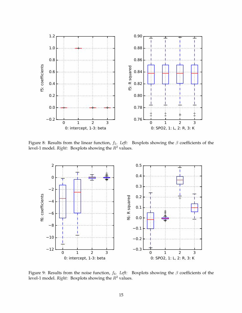
1. The first boxplots (on left in each figure) show the coefficients of the level-1 linear model,i.e., the first entry represents the value of the intercept or β0. Three additional boxplotsare shown to visualize the effect of the single models, i.e., values of the coefficients β1(linear model), β2 (random forest), and β3 (Gaussian process model, Kriging) are shown.

10

4 3 2 1 0 1 2 3 44

2

0

2

4

6

f1

4 3 2 1 0 1 2 3 42

0

2

4

6

8

f2

4 3 2 1 0 1 2 3 4

4

2

0

2

4

f3

4 3 2 1 0 1 2 3 486420246

f4

4 3 2 1 0 1 2 3 486420246

f5

4 3 2 1 0 1 2 3 46543210123

f6

Figure 3: Plots of the six test functions. First row, from left to right: Step function f1, polynomialfunction f2, sine function f3. Second row, from left to right: Combined function f4, linear functionf5, random function f6. Blue lines illustrate the true function, red dots represent (noisy) samplespresented to the approximation models.

2. The second set of boxplots (on the right in each figure) show the performance of the fourdifferent modeling approaches, i.e., SPO2 (0), linear model (1), random forest (2), andGaussian process model (3).

This arrangement of boxplots should reveal correlations between the β values from the level-1model and the R2 performance.

While analyzing the results from the step function, f1, the boxplots indicate that randomforest outperforms the other modeling approaches (Fig. 4). Slightly worse results were ob-tained by the Gaussian process models, whereas the linear model performs worse. The SPO2ensemble engine was able to identify the good performers. The random forest coefficient, i.e.,β2 is the largest coefficient in the level-1 model.

While analyzing the results on the polynomial function, f2, the outcome is unambiguous(Fig. 5). The Gaussian process model exhibits the best performance, and the random forestperforms equally well. The linear model is not able to find a good fit. This situation is reflectedin the values of coefficients of the level-1 model: the β3 values, which are associated withthe Gaussian process model, are high, whereas the values of the remaining β coefficients arenegligible. A similar situation occurs during the results on the sine function, f3 (Fig. 6).

Results from the combined function are more interesting (Fig. 7). Here, the random forestmodel results in the best fit (with respect to the R2 error). The second best model, i.e., theGaussian process model, performs better than the linear model. This ranking is mirrored inthe values of the β coefficients.

Since the linear model was always the worst model, it might be of interest to see if thisobservation still holds for the approximation of data which have a simple linear relationship.a linear model. Therefore, test function f5 was added to the test function portfolio from [45].Every model was able to generate a good approximation as can be seen in Fig. 8. Interestingly,the SPO2 engine prefers the linear function as can be seen from the values of the β1 coefficient.

11

Finally, to present a situation where every approximation must fail, a purely random func-tion with additional noise was added to our portfolio (Fig. 9). The boxplots shown that nomodel was able get a good R2 value. The ensemble approach fails completely in this setting.

7 Summary and Outlook

This study nicely illustrates some important benefits of the stacked generalization approach:• Combining model information, even from models with poor approximation capabilities,

might result in an improved approximation.• Combining model information results only in a small performance decrease, if the port-

folio contains a good performing modelThe question, why ensembles perform better, is the subject of on-going research. Results

from this study indicate, that the stacked generalization approach might work. However, thisis not a proof, only an indication that it might be worth going into this direction. An extendedstudy, which compares more surrogate models and includes more test functions, will be pub-lished soon.

The good performance of the ensemble approach does not come for free. The additionalevaluations slow down the modeling process. In situations, where no information about thestructure of the fitness landscape is available, the stacked generalization approach might be anadequate first choice. Models can be added or deleted from the portfolio dynamically duringthe search.

Acknowledgement

This work has been supported by the Bundesministeriums für Wirtschaft und Energie under thegrants KF3145101WM3 und KF3145103WM4. This work is part of a project that has receivedfunding from the European Union’s Horizon 2020 research and innovation program under grantagreement No 692286.

12

0 1 2 3

0: intercept, 1-3: beta

0.4

0.2

0.0

0.2

0.4

0.6

0.8

1.0

1.2

1.4

f1:

coeff

icie

nts

0 1 2 3

0: SPO2, 1: L, 2: R, 3: K

0.1

0.2

0.3

0.4

0.5

0.6

0.7

0.8

0.9

f1:

R s

quare

d

Figure 4: Results from the step function, f1. Left: Boxplots showing the β coefficients of the level-1model. Right: Boxplots showing the R2 values.

0 1 2 3

0: intercept, 1-3: beta

0.2

0.0

0.2

0.4

0.6

0.8

1.0

1.2

f2:

coeff

icie

nts

0 1 2 3

0: SPO2, 1: L, 2: R, 3: K

0.0

0.1

0.2

0.3

0.4

0.5

0.6

0.7

0.8

0.9

f2:

R s

quare

d

Figure 5: Results from the polynomial function, f2. Left: Boxplots showing the β coefficients ofthe level-1 model. Right: Boxplots showing the R2 values.

13

0 1 2 3

0: intercept, 1-3: beta

0.2

0.0

0.2

0.4

0.6

0.8

1.0

1.2

f3:

coeff

icie

nts

0 1 2 3

0: SPO2, 1: L, 2: R, 3: K

0.0

0.1

0.2

0.3

0.4

0.5

0.6

0.7

0.8

0.9

f3:

R s

quare

d

Figure 6: Results from the sine function, f3. Left: Boxplots showing the β coefficients of the level-1model. Right: Boxplots showing the R2 values.

0 1 2 3

0: intercept, 1-3: beta

7

6

5

4

3

2

1

0

1

2

f4:

coeff

icie

nts

0 1 2 3

0: SPO2, 1: L, 2: R, 3: K

0.0

0.2

0.4

0.6

0.8

f4:

R s

quare

d

Figure 7: Results from the combined function, f4. Left: Boxplots showing the β coefficients of thelevel-1 model. Right: Boxplots showing the R2 values.

14

0 1 2 3

0: intercept, 1-3: beta

0.2

0.0

0.2

0.4

0.6

0.8

1.0

1.2

f5:

coeff

icie

nts

0 1 2 3

0: SPO2, 1: L, 2: R, 3: K

0.76

0.78

0.80

0.82

0.84

0.86

0.88

0.90

f5:

R s

quare

d

Figure 8: Results from the linear function, f5. Left: Boxplots showing the β coefficients of thelevel-1 model. Right: Boxplots showing the R2 values.

0 1 2 3

0: intercept, 1-3: beta

12

10

8

6

4

2

0

2

f6:

coeff

icie

nts

0 1 2 3

0: SPO2, 1: L, 2: R, 3: K

0.3

0.2

0.1

0.0

0.1

0.2

0.3

0.4

0.5

f6:

R s

quare

d

Figure 9: Results from the noise function, f6. Left: Boxplots showing the β coefficients of thelevel-1 model. Right: Boxplots showing the R2 values.

15

References

[1] Alessandro Baldi Antognini and Maroussa Zagoraiou. Exact optimal designs for com-puter experiments via Kriging metamodelling. Journal of Statistical Planning and Inference,140(9):2607–2617, September 2010.

[2] Thomas Bartz-Beielstein, Christian Lasarczyk, and Mike Preuß. Sequential Parameter Op-timization. In B McKay et al., editors, Proceedings 2005 Congress on Evolutionary Computa-tion (CEC’05), Edinburgh, Scotland, pages 773–780, Piscataway NJ, 2005. IEEE Press.

[3] Thomas Bartz-Beielstein, Konstantinos E Parsopoulos, and Michael N Vrahatis. Designand analysis of optimization algorithms using computational statistics. Applied NumericalAnalysis and Computational Mathematics (ANACM), 1(2):413–433, 2004.

[4] Andrew J Booker, J E Dennis Jr, Paul D Frank, David B Serafini, and Virginia Torczon.Optimization Using Surrogate Objectives on a Helicopter Test Example. In ComputationalMethods for Optimal Design and Control, pages 49–58. Birkhäuser Boston, Boston, MA, 1998.

[5] G E P Box and N R Draper. Empirical Model Building and Response Surfaces. Wiley, NewYork NY, 1987.

[6] L Breiman, J H Friedman, R A Olshen, and C J Stone. Classification and Regression Trees.Wadsworth, Monterey CA, 1984.

[7] D Büche, N N Schraudolph, and P Koumoutsakos. Accelerating Evolutionary AlgorithmsWith Gaussian Process Fitness Function Models. IEEE Transactions on Systems, Man andCybernetics, Part C (Applications and Reviews), 35(2):183–194, May 2005.

[8] Ivo Couckuyt, Filip De Turck, Tom Dhaene, and Dirk Gorissen. Automatic surrogatemodel type selection during the optimization of expensive black-box problems. In 2011Winter Simulation Conference - (WSC 2011), pages 4269–4279. IEEE, 2011.

[9] Michael Emmerich, Alexios Giotis, Mutlu özdemir, Thomas Bäck, and Kyriakos Gian-nakoglou. Metamodel-assisted evolution strategies. In J J Merelo Guervós, P Adamidis,H G Beyer, J L Fernández-Villacañas, and H P Schwefel, editors, Parallel Problem Solvingfrom Nature—PPSN VII, Proceedings~Seventh International Conference, Granada, pages 361–370, Berlin, Heidelberg, New York, 2002. Springer.

[10] Alexander Forrester, András Sóbester, and Andy Keane. Engineering Design via SurrogateModelling. Wiley, 2008.

[11] Alexander I J Forrester and Andy J Keane. Recent advances in surrogate-based optimiza-tion. Progress in Aerospace Sciences, 45(1-3):50–79, January 2009.

[12] K B Wilson G E P Box. On the Experimental Attainment of Optimum Conditions. Journalof the Royal Statistical Society. Series B (Methodological), 13(1):1–45, 1951.

[13] K C Giannakoglou. Design of optimal aerodynamic shapes using stochastic optimiza-tion methods and computational intelligence. Progress in Aerospace Sciences, 38(1):43–76,January 2002.

[14] Tushar Goel, Raphael T Haftka, Wei Shyy, and Nestor V Queipo. Ensemble of surrogates.Struct. Multidisc. Optim., 33(3):199–216, September 2006.

[15] Robert B Gramacy. tgp: An R Package for Bayesian Nonstationary, Semiparametric Non-linear Regression and Design by Treed Gaussian Process Models. Journal of StatisticalSoftware, 19(9):1–46, June 2007.

[16] P Hajela and E Lee. Topological optimization of rotorcraft subfloor structures for crash-worthiness considerations. Computers & Structures, 64(1-4):65–76, July 1997.

[17] Trevor Hastie. The elements of statistical learning : data mining, inference, and prediction.Springer, New York, 2nd ed. edition, 2009.

[18] Mark Hauschild and Martin Pelikan. An introduction and survey of estimation of distri-bution algorithms. Swarm and Evolutionary Computation, 1(3):111–128, September 2011.

16

[19] Jiaqiao Hu, Yongqiang Wang, Enlu Zhou, Michael C Fu, and Steven I Marcus. A Survey ofSome Model-Based Methods for Global Optimization. In Daniel Hernández-Hernándezand J Adolfo Minjárez-Sosa, editors, Optimization, Control, and Applications of StochasticSystems, pages 157–179. Birkhäuser Boston, Boston, 2012.

[20] Edward Huang, Jie Xu, Si Zhang, and Chun Hung Chen. Multi-fidelity Model Integrationfor Engineering Design. Procedia Computer Science, 44:336–344, 2015.

[21] Frank Hutter, Holger Hoos, and Kevin Leyton-Brown. An Evaluation of SequentialModel-based Optimization for Expensive Blackbox Functions. In Proceedings of the 15thAnnual Conference Companion on Genetic and Evolutionary Computation, pages 1209–1216,New York, NY, USA, 2013. ACM.

[22] R Jin, W Chen, and T W Simpson. Comparative studies of metamodelling techniquesunder multiple modelling criteria. Struct. Multidisc. Optim., 23(1):1–13, December 2001.

[23] Y Jin. A comprehensive survey of fitness approximation in evolutionary computation.Soft Computing, 9(1):3–12, October 2003.

[24] Y Jin, M Olhofer, and B Sendhoff. On Evolutionary Optimization with Approximate Fit-ness Functions. GECCO, 2000.

[25] D R Jones, M Schonlau, and W J Welch. Efficient Global Optimization of Expensive Black-Box Functions. Journal of Global Optimization, 13:455–492, 1998.

[26] Jack P C Kleijnen. Kriging metamodeling in simulation: A review. European Journal ofOperational Research, 192(3):707–716, February 2009.

[27] P Larraaga and J A Lozano. Estimation of Distribution Algorithms. A New Tool for Evolution-ary Computation. Kluwer, Boston MA, 2002.

[28] Minh Nghia Le, M N Le, Yew Soon Ong, Y S Ong, S Menzel, Stefan Menzel, Yaochu Jin,Y Jin, B Sendhoff, and Bernhard Sendhoff. Evolution by adapting surrogates. EvolutionaryComputation, 21(2):313–340, 2013.

[29] S N Lophaven, H B Nielsen, and J Søndergaard. DACE—A Matlab Kriging Toolbox.Technical report, 2002.

[30] J Mockus, V Tiesis, and A Zilinskas. Bayesian Methods for Seeking the Extremum. InL C W Dixon and G P Szegö, editors, Towards Global Optimization, pages 117–129. Amster-dam, 1978.

[31] D C Montgomery. Design and Analysis of Experiments. Wiley, New York NY, 5th edition,2001.

[32] K P Murphy. Machine learning: a probabilistic perspective, 2012.

[33] Andrea Nelson, Juan Alonso, and Thomas Pulliam. Multi-Fidelity Aerodynamic Opti-mization Using Treed Meta-Models. In Fluid Dynamics and Co-located Conferences. Ameri-can Institute of Aeronautics and Astronautics, Reston, Virigina, June 2007.

[34] Emanuele Olivetti. blend.py, 2012. Code available on https://github.com/emanuele/kaggle_pbr/blob/master/blend.py. Published under a BSD 3 license.

[35] MJD Powell. Radial Basis Functions. Algorithms for Approximation, 1987.

[36] Mike Preuss. Multimodal Optimization by Means of Evolutionary Algorithms. Natural Com-puting Series. Springer International Publishing, Cham, 2015.

[37] F Pukelsheim. Optimal Design of Experiments. Wiley, New York NY, 1993.

[38] Nestor V Queipo, Raphael T Haftka, Wei Shyy, Tushar Goel, Rajkumar Vaidyanathan, andP Kevin Tucker. Surrogate-based analysis and optimization. Progress in Aerospace Sciences,41(1):1–28, January 2005.

[39] Alain Ratle. Parallel Problem Solving from Nature — PPSN V: 5th International Con-ference Amsterdam, The Netherlands September 27–30, 1998 Proceedings. pages 87–96.Springer Berlin Heidelberg, Berlin, Heidelberg, 1998.

17

[40] Margarita Alejandra Rebolledo Coy, Sebastian Krey, Thomas Bartz-Beielstein, OliverFlasch, Andreas Fischbach, and Jörg Stork. Modeling and Optimization of a Robust GasSensor. Technical Report 03/2016, Cologne Open Science, Cologne, 2016.

[41] T J Santner, B J Williams, and W I Notz. The Design and Analysis of Computer Experiments.Springer, Berlin, Heidelberg, New York, 2003.

[42] M Schonlau. Computer Experiments and Global Optimization. PhD thesis, University ofWaterloo, Ontario, Canada, 1997.

[43] L Shi and K Rasheed. A Survey of Fitness Approximation Methods Applied in Evolu-tionary Algorithms. In Computational Intelligence in Expensive Optimization Problems, pages3–28. Springer Berlin Heidelberg, Berlin, Heidelberg, 2010.

[44] G Sun, G Li, S Zhou, W Xu, X Yang, and Q Li. Multi-fidelity optimization for sheet metalforming process. Structural and Multidisciplinary . . . , 2011.

[45] M J van der Laan and E C Polley. Super Learner in Prediction. UC Berkeley Division ofBiostatistics Working Paper . . . , 2010.

[46] V N Vapnik. Statistical learning theory. Wiley, 1998.

[47] G Gary Wang and S Shan. Review of Metamodeling Techniques in Support of EngineeringDesign Optimization. Journal of Mechanical . . . , 129(4):370–380, 2007.

[48] David H Wolpert. Stacked generalization. Neural Networks, 5(2):241–259, January 1992.

[49] Luis E Zerpa, Nestor V Queipo, Salvador Pintos, and Jean-Louis Salager. An optimizationmethodology of alkaline–surfactant–polymer flooding processes using field scale numer-ical simulation and multiple surrogates. Journal of Petroleum Science . . . , 47(3-4):197–208,June 2005.

[50] Z Zhou, Y S Ong, P B Nair, A J Keane, and K Y Lum. Combining Global and LocalSurrogate Models to Accelerate Evolutionary Optimization. IEEE Transactions on Systems,Man and Cybernetics, Part C (Applications and Reviews), 37(1):66–76, 2007.

[51] Mark Zlochin, Mauro Birattari, Nicolas Meuleau, and Marco Dorigo. Model-Based Searchfor Combinatorial Optimization: A Critical Survey. Annals of Operations Research, 131(1-4):373–395, 2004.

[52] J M Zurada. Analog implementation of neural networks. IEEE Circuits and Devices Maga-zine, 8(5):36–41, 1992.

18

CIplus Band 5/2016

Stacked Generalization of Surrogate Models - A Practical Approach Technischer Bericht / Technical Report Prof. Dr. Thomas Bartz-Beielstein Institut für Informatik Fakultät für Informatik und Ingenieurwissenschaften Technische Hochschule Köln Mai 2016

Die Verantwortung für den Inhalt dieser Veröffentlichung liegt beim Autor.