The University of Southern Mississippi The University of Southern Mississippi

The Aquila Digital Community The Aquila Digital Community

Master's Theses

Fall 2019

Localized Method Of Approximate Particular Solutions For Localized Method Of Approximate Particular Solutions For

Solving Optimal Control Problems Governed By PDES Solving Optimal Control Problems Governed By PDES

Kwesi Acheampong University of Southern Mississippi

Follow this and additional works at: https://aquila.usm.edu/masters_theses

Recommended Citation Recommended Citation Acheampong, Kwesi, "Localized Method Of Approximate Particular Solutions For Solving Optimal Control Problems Governed By PDES" (2019). Master's Theses. 678. https://aquila.usm.edu/masters_theses/678

This Masters Thesis is brought to you for free and open access by The Aquila Digital Community. It has been accepted for inclusion in Master's Theses by an authorized administrator of The Aquila Digital Community. For more information, please contact Joshua.Cromwell@usm.edu.

LOCALIZED METHOD OF APPROXIMATE PARTICULAR SOLUTIONS FOR

SOLVING OPTIMAL CONTROL PROBLEMS GOVERNED BY PDES

by

Kwesi Asante Acheampong

A ThesisSubmitted to the Graduate School,the College of Arts and Sciences

and the School of Mathematics and Natural Sciencesof The University of Southern Mississippiin Partial Fulfillment of the Requirements

for the Degree of Masters of Science

Approved by:

Dr. Huiqing Zhu, Committee ChairDr. Haiyan TianDr. C.S. Chen

Dr. Huiqing Zhu Dr. Bernd Schroeder Dr. Karen S. CoatsCommittee Chair Director of School Dean of the Graduate School

December 2019

COPYRIGHT BY

KWESI ASANTE ACHEAMPONG

2019

ABSTRACT

In this thesis, the method of approximate particular solutions(MAPS) and localized

method of approximate particular solutions(LMAPS) with polynomial basis, and radial basis

functions are proposed and applied on the optimal control problems(OCPs) governed by

partial differential equations(PDEs).

This study proceeds in several steps. First, polynomial basis and radial basis functions

are used to globally approximate solutions for the PDEs which have been combined into a

single matrix system numerically from the optimality conditions of the OCPs. Secondly,

polynomial and radial basis functions are used to locally approximate particular solutions

for the same matrix system numerically. We use these approaches to two types of problems,

a smooth and singular problem. The first example numerically experiments on a square

domain and the second example on an L-shaped disc domain. These approaches are tested

and compared. The results show our proposed method for solving optimal control problems

governed by partial differential equations works.

ii

ACKNOWLEDGMENTS

I would like to thank all of those who have assisted me in this effort of my master’s

degree thesis. First of all, I would like to thank my advisor, Dr. Zhu, for all of the time and

relentless effort he gave in working with me on my thesis. This has taught me a lot of lessons

from him and not only mathematics and coding, but also about the research procedures. I

am extremely grateful to him for all that he has taught me over the past one and a half year,

and for his patience, encouragement, and advice throughout this process.

Also, I would like to thank my thesis defense committee from the Department of

Mathematics- Prof. Chen, and Dr. Tian. I profoundly appreciate all of opinions, questions,

and comments that I received on this research.

In addition, I would like to thank Dr. Guan from the Zhengzhou University of Light

Industry in China for introducing and making me understand optimally controlled problems

in mathematics. I thank Dr. Lambers, Dr. Jaeyoun Oh, Dr. Brianna Bingham and Dr. Hailey

Bates of the University of Southern Mississippi’s Department of Mathematics for providing

emotional support and assistance in my thesis and also helping me know the required things

to do to help me graduate. I would also like to thank my family, my mom, dad, siblings, for

all of their immense love and support throughout this process and throughout my master’s

degree. I could not have gotten this far without all that they have done for me.

Finally, I would like to thank Christian, Xavier, Dr. Ackablay Martha, Krystle, Theresa,

Christen, Miss Pattie, Cyril, Lionel, Subagya, Peace, Mona, Precious, Mariam, Promise,

Grace, all my African brothers and sisters and my other friends who provided me with fun

times and great memories to keep me going through tough times. It was really a blessing for

having them in my life and I really appreciate everything you did for me .

iii

TABLE OF CONTENTS

ABSTRACT . . . . . . . . . . . . . . . . . . . . . . . . . . . . . . . . . . ii

ACKNOWLEDGMENTS . . . . . . . . . . . . . . . . . . . . . . . . . . . . iii

LIST OF ILLUSTRATIONS . . . . . . . . . . . . . . . . . . . . . . . . . . v

LIST OF TABLES . . . . . . . . . . . . . . . . . . . . . . . . . . . . . . . vi

LIST OF ABBREVIATIONS . . . . . . . . . . . . . . . . . . . . . . . . . vii

NOTATION AND GLOSSARY . . . . . . . . . . . . . . . . . . . . . . . . viii

1 BACKGROUND . . . . . . . . . . . . . . . . . . . . . . . . . . . . . . 11.1 Introduction 11.2 Optimal Control Problems 11.3 A Brief Literature Review 31.4 Aim of this Study 4

2 GLOBAL METHOD OF APPROXIMATE PARTICULAR SOLUTIONS . 52.1 Introduction of Method of Approximated Particular Solutions For Poisson Equa-tion 52.2 Method of Approximated Particular Solutions Scheme for Optimal ControlProblems 82.3 Numerical experiments 10

3 LOCALIZED METHOD OF APPROXIMATE PARTICULAR SOLUTIONS 173.1 Introduction of Local Method of Approximated Particular Solutions For PoissonEquation 183.2 Localized Method of Approximate Particular Solutions Scheme for OptimalControl Problems 203.3 Numerical experiments 21

4 CONCLUSIONS AND REMARKS . . . . . . . . . . . . . . . . . . . . . 27

BIBLIOGRAPHY . . . . . . . . . . . . . . . . . . . . . . . . . . . . . . . 28

iv

LIST OF ILLUSTRATIONS

Figure

2.1 Square Domain . . . . . . . . . . . . . . . . . . . . . . . . . . . . . . . . . . 112.2 L-shaped Disc Domain . . . . . . . . . . . . . . . . . . . . . . . . . . . . . . 112.3 16×16 square domain . . . . . . . . . . . . . . . . . . . . . . . . . . . . . . 122.4 RMSE errors of y and u of MAPS with both RBFs and Polynomial basis. . . . 142.5 860 collocation points on a L-shape disc domain . . . . . . . . . . . . . . . . . 152.6 RMSE errors of y and p of MAPS with both RBFs and Polynomial basis. . . . 16

3.1 RMSE errors of y and u of LMAPS with both RBFs and Polynomial basis. . . . 243.2 RMSE errors of y and p of LMAPS with both RBFs and Polynomial basis. . . . 26

v

LIST OF TABLES

Table

2.1 Commonly used RBF’s . . . . . . . . . . . . . . . . . . . . . . . . . . . . . . 62.2 The Particular Solution of MQ RBF for the Laplace operator in this study . . . 62.3 Root Mean Square Errors of y and u for using RBFs . . . . . . . . . . . . . . . 132.4 Root Mean Square Errors of y and u for using Polynomial Basis . . . . . . . . 132.5 Root Mean Square Errors of y and p for using RBFs . . . . . . . . . . . . . . . 162.6 Root Mean Square Errors of y and p for using Polynomial Basis . . . . . . . . 16

3.1 Root Mean Square Errors of y and u for using RBFs . . . . . . . . . . . . . . . 233.2 Root Mean Square Errors of y and u for using Polynomial Basis . . . . . . . . 243.3 Root Mean Square Errors y and p for using RBFs . . . . . . . . . . . . . . . . 253.4 Root Mean Square Errors y and p for using Polynomial Basis . . . . . . . . . . 26

vi

LIST OF ABBREVIATIONS

RBF - Radial Basis FunctionMQ - Multiquadrics

OCP - Optimal Control ProblemsRMSE - Root Mean Square Error

IMQ - Inverse MultiquadricsPDE - Partial Differential Equation

MAPS - Method of Approximate Particular SolutionsLMAPS - Localized Method of Approximate Particular Solutions

FEM - Finite Element MethodFDM - Finite Difference Method

vii

NOTATION AND GLOSSARY

General Usage and Terminology

The several notation used in this thesis represents fairly standard mathematical and com-putational usage. The methods used in this study have interdisciplinary applications, andin this particular study is being centered around partial differential equations.In severalcases these fields tend to use different preferred notation to indicate the same idea. While itwould be convenient to utilize a standard nomenclature for this important symbol, the manyalternatives currently in the published literature will continue to be utilized.

These blackboard fonts are used to denote standard sets of numbers: R for the field ofreal numbers. The capital letters, A,P,L,F, · · · are used to denote matrices in the globalmethod. Boldface capital letter P represents polynomial space. Also, capital boldfacedgreek letters, e.g., Θ ,Ψ for matrices in the local method. Functions which are denoted inboldface type typically represent vector valued functions, and real valued functions usuallyare set in lower case roman letters e.g., f ,g. Caligraphic letters L,B are used to denotepartial differential operators. Again, lower case roman letters e.g.,k,n,s, j are used to denoteindices.

Vectors and matrices are typeset in square brackets, e.g., [·], and parenthesis, e.g., (·). Ingeneral the norms are typeset using double pairs of lines, e.g., || · ||.

viii

1

Chapter 1

BACKGROUND

1.1 Introduction

The use of differential equation applications has become rampant in various fields in theworld like engineering, biology, physics, computational mathematics, and economics. Dueto this, it has become necessary to solve these differential equations analytically but mostof these differential equations problems cannot be solved analytically. Therefore, it hasbecome expedient to find other ways to solve these kinds of equations. Researchers foundseveral methods of numerically solving these problems by approximating their solutions.

In this thesis, we focus is on optimal control problems governed by PDEs. Optimalcontrol theory was developed by Lev Semenovic Pontryagin and his colleagues in thelate 1950s, which generalizes the calculus of variations. This optimal control for finitedimensional problems is derived by using the Pontryagin’s maximum principle which isgoverned by ordinary differential equations [10,14,16]. J. L. Lions developed the optimalcontrol system theory governed by PDEs [10,13]. Pontryagin’s maximum principles areused to help characterize an optimal control problem via an optimality system, whichincludes the state and adjoint system. When the optimal controls and its state variables aregiven, there are adjoint variables, which satisfy the system. With this concept, the sourceterms of the adjoint PDEs equal the partial derivatives of the integrand of the objectivefunction with respect to the state variables [10,26]. For some decades now optimal controlproblems governed by partial differential equations have become an area of interest byresearchers because of its application to real-world problems. Some of these applicationsinclude optimizing the cooling process of hot steel [8,12], pollutant control in a river [5,8]and magnetic drug targeting [6,8].

This chapter will introduce us to the optimal control problem in this study. This chapterwill also discuss some of the works that have been done on this problem over the years andthe aim of this study.

1.2 Optimal Control Problems

In this section, we discuss optimal control problems in detail but the kind of partial differen-tial equation we will discuss in this research is the Poisson equation. Poisson equations are

2

elliptic partial differential equation problems and have the form

∆u = uxx +uyy = f (x,y). (1.1)

In [11], the paper mentions two of the problems. These problems are the distributivecontrol problem and boundary control problem. The distributive control problem means thecontrolling is being done in the domain. While the boundary control problem means thecontrolling is being done only on the boundary. This study focuses just on the distributedcontrol problem. Optimizing a quantity with Poisson equation as a constraint, one can call ita Poisson control problem. This is one of the most commonly PDE-constrained optimizationproblems researched.

The problem we consider in this study is of the form

miny,u

12‖y− y‖2

L2(Ω)+β

2‖u‖2

L2(Ω) (1.2)

such that−∆y = u, in Ω,

y = f , on ∂Ω,

for some penalty constant β > 0. β ’s value is very important, so if it is small, then y

being far away from y is penalized heavily [11]. If β is large, it is very important u hassmall L2(Ω). We define y to be the state variable and u to be the control variable in theentire domain(Ω) and y is the optimality state. Ω is a two dimension bounded domain. y

and u are continuous functions, y ∈ H1(Ω) and u ∈ L2(Ω) [11]. To solve this problem(1.2), there are two approaches, which are the discretize-then-optimize formulation andthe optimize-then-discretize formulation of the distributed control problem in [11]. Weuse the optimize-then-discretize formulation idea in [11]. The importance of using thisapproach is to come up with a Lagrangian on the continuous space, get optimality con-ditions and discretize it finally. The Lagrangian L = L(y,u, p1, p2) on the continuous space is

L =12‖y− y‖2

L2(Ω)+β

2‖u‖2

L2(Ω)+∫

Ω

(−∆y−u)p1dΩ+∫

∂Ω

yp2ds, (1.3)

where, p1 represents continuous adjoint variable in the domain(Ω), p2 represents the con-tinuous adjoint variable on the boundary(∂Ω). Take note that p in general denotes thecontinuous adjoint variable and also performs the same role as the Lagrange multipliers insection 3.1 of Pearson’s paper [11,18].

3

The Lagrangian(1.3) is differentiated with respect to the continuous variables u,y and p.This results in getting the optimality conditions, which are, the State equation:

−∆y = u, in Ω, (1.4)

y = f , on ∂Ω,

the Gradient equation:

βu− p = 0, in Ω, (1.5)

u = 0, on ∂Ω,

the Adjoint equation:

−∆p = y− y, in Ω, (1.6)

p = 0, on ∂Ω.

For a full understanding of this derivation of these conditions, one should refer to [11,18,23].These optimality conditions are discretized in section 2.2 for the global method and section3.2 for the local method to form a system of a matrix.

1.3 A Brief Literature Review

For some years now several methods have been used to solve optimal control problems dueto its various applications in the aerodynamic, medical, biological, finance and engineeringfields. Distributed control problems governed by PDEs are generally difficult to obtaintheir analytical solution [15]. Sometimes the exact solutions of these problems are notavailable, therefore, the applications of many traditional numerical procedures, for example,finite element method (FEM), finite difference method (FDM) are used to approximatetheir solutions. In [19], they transformed the control problem into a two boundary problem.They also, integrated the generalized orthogonal polynomials to get an operational matrixand then used Taylor series, lots of orthogonal polynomials to obtain the optimal control,by using only the cross-product Legendre vectors. Apel et. al [21], solves an optimalcontrol problem for a two-dimensional elliptic equation with point wise control constraintsand the domain used is assumed to be a polygon but non-convex. They treat the corner

4

singularities by prior mesh grading and the approximations of the solutions are constructedby a projection of the discrete adjoint state. They again prove that the approximations have aconvergence order of h2. In [24], they solved a Dirichlet boundary control problem by usinga Mixed finite element method. This paper [25] uses a convergent adaptive finite elementmethod for elliptic Dirichlet boundary control problems. Pearson’s article uses a radial basisfunction method to solve PDE-constrained problems (that is Poisson equations), he derivesnew collocation-type methods to solve distributed control problems that have Dirichletboundary conditions and also extends it to Neumann boundary conditions problem. Againhe proves the results pertaining to invertibility of the matrix he generates. These methods areimplemented using MATLAB and produce numerical results to exhibit the capability of themethod in his article [11]. For Darehmiraki’s paper, he presents a reproducing kernel Hilbertspaces method to get numerical solutions for the optimal control problem. He approximatedthe solution by truncating the series form of the analytical solution in the reproducingkernel space [15]. In this paper [25] uses a convergent adaptive finite element method forelliptic Dirichlet boundary control problems. This paper [7] proposes a nonconforming finiteelement method to solve an optimal control problem governed by the bilinear state equation.They approximate the state and adjoint equation by using a nonconforming EQrot

1 element,and the control is approximated by orthogonal projection through the state and adjoint state.Superconvergence and super close properties are obtained by full use of the characters ofthis EQrot

1 element and the consistency error is one order higher than its interpolation error.Guan et. al in [8], uses two meshless scheme for solving Dirichlet boundary optimal controlproblems governed by elliptic equations. They use a radial basis function collocation methodfor both state and adjoint state equations in the first scheme, and in the second scheme, theyemploy the method of fundamental solutions for the state equation when it has a zero sourceterm, and radial basis function collocation method for the adjoint state equation.

1.4 Aim of this Study

This study will solve the optimal control problem (1.4) with Dirichlet boundary conditionson a square domain and L-shape disc domain by using global and localized method ofapproximate solutions with radial basis functions and polynomial basis. This study wasmotivated by Pearson’s paper [11], who used Global Kansas Method with RBFs and alsoCompact Supported RBFs. Based on the method he used, I considered MAPS and LMAPS.

5

Chapter 2

GLOBAL METHOD OF APPROXIMATE PARTICULARSOLUTIONS

There are several methods of numerically solving partial differential equations. One of themethods discussed in this chapter is the method of approximate particular solutions with theuse of radial basis functions(RBFs) and polynomial basis. This is a meshless method used tosolve the large size of partial differential equations in engineering and the sciences. Radialbasis functions used in solving partial differential equations are simple and can be appliedto various PDEs. It is effective in dealing with high dimensions problems with sophisticatedgeometries. Polynomial basis, on the other hand, can be used to approximate solutions toPDEs because sometimes it is not convenient to choose a shape parameter in RBF functionsfor finding a particular solution for a differential operator governing an equation.In this chapter we will introduce MAPS for Poisson equation, MAPS solutions scheme forOptimal Control Problems and then talk about the numerical experiments.

2.1 Introduction of Method of Approximated Particular Solutions For PoissonEquation

This section, we will lay more emphasis on the basis and the method we are going to use toapproximate the particular solution for a differential operator(L). We define RBFs as: letRd with d being the dimensional Euclidean space. A function h: Rd → R is a radial whenthere exist a univariate function φ : [0,∞)→ R such that

h(x) = φ(r),

where r is the Euclidean norm of x, that is r = ‖x‖. The table below shows some commonlyused RBFs.

6

Table 2.1: Commonly used RBF’s.

RBF’s Names Formulations

linear φ(r) = r

cubic φ(r) = r3

Gaussian φ(r) = e−cr2,c > 0

Multiquadrics(MQ) φ(r) =√

r2c2 +1,c > 0

Inverse Multiquadrics(IMQ) φ(r) =1√

r2c2 +1,c > 0

Thine-plate spline (TPD) φ(r) = r2ln(r)

For MAPS, a solution, Φ(r), for a particular differential equation is to be known:

LΦ(r) = φ(r).

Table 2.2 shows the closed forms of solutions used as basis functions to approximatesolutions of the given PDE under study, and the RBF used is Multiquadrics(MQ). Thepositive constant c in Table 2.1 and Table 2.2 denotes the shape parameter of the RBF.

Table 2.2: The Particular Solution of MQ RBF for the Laplace operator in this study.

Φ(r) =2c2

√c2r2 +1

− c4r2

(√

c2r2 +1)3

The use of polynomial basis function as particular solutions for a differential operatorequation is unstable as the degree of the polynomial is being increased. It is unstable becausethe resultant matrix becomes ill-conditioned due to how dense the matrix is. Therefore,polynomial basis functions for approximating our closed-form particular solutions are notgood for a global approach unless there is a proper treatment of our matrix resulting fromour formulation. There are several types of preconditioning treatments for the matrix but theone used in this thesis is called the multi-scale technique. It is used to reduce the conditionnumber of the method of approximated particular solutions resultant matrix. For a standardpolynomial basis for a 2D case, finding the particular solutions for a differential operator(L)of an equation, we choose a sequence of polynomials

pn(x,y) = xi− jy j, 0≤ j ≤ i, 0≤ i≤ k, 1≤ n≤ w, ∀(x,y) ∈ R2.

7

This sequence forms a basis for the polynomial space Prk, the set r-variate polynomials of

degree ≤ k,and r = 2. The dimension of the polynomial space Prk is w =

(k+1)(k+2)2

.From Thir Raj Dangal’s dissertation in 2017[22], a simple example was used to find theparticular solution. A conclusion was drawn that the procedure used for finding the particularsolution can be extended to find the particular solution for the polynomial functions for anygeneral differential operator.

Theorem 2.1.1. Consider a general form second-order linear partial differential equation

in two variables with constant coefficients:

a1∂ 2up

∂x2 +a2∂ 2up

∂x∂y+a3

∂ 2up

∂y2 +a4∂up

∂x+a5

∂up

∂y+a6up = xmyn, (2.1)

where ai6i=1 are real constants, a6 6= 0 and m and n are positive integers. Then the

polynomial particular solution of (2.1) is given by

up =1a6

N

∑k=0

(−1a6

)k

Lk(xmyn), (2.2)

where N = m+n and

L= a1∂ 2

∂x2 +a2∂ 2

∂x∂y+a3

∂ 2

∂y2 +a4∂

∂x+a5

∂

∂y.

The proof of this theorem can be again found in Thir Raj Dangal’s dissertation in 2017[22].Now that we done talking about ways of getting the particular solutions, we consider a

PDE, which in this paper is a Poisson equation but we would like to use a general differentialoperator.

Lu(x) = f (x), x ∈Ω, (2.3)

u(x) = g(x), x ∈ ∂Ω. (2.4)

We then use the two discussed particular solutions above to solve this problem by generaliz-ing this particular solution to fit for both types of particular solution. The approximation u

to the exact solution u in (2.3) and (2.4) is

u(x)≈ u(x) =N

∑k=1

αkΦk, (2.5)

8

where Φ denotes the closed form solutions used as basis functions to approximate solutionsof the given PDEs for RBF or polynomial basis i.e LΦ(r) = φ(r) and below is somenotations we need to know.

• xkN1 the set of all collocation points.

• xkNi1 the set of interior points.

• xkNi+NbNi+1 the set of boundary points.

and N = Ni +Nb. Next we substitute (2.5) into (2.3) and (2.4):

Lu(x) =N

∑k=1

αkLΦk = f (x), x ∈Ω, (2.6)

u(x) =N

∑k=1

αkΦk = g(x), x ∈ ∂Ω. (2.7)

Then linear system (2.6) and (2.7) is discretized on collocation points to form a system ofmatrices with a coefficient α:

Aα =C, (2.8)

where α = [α1,α2 · · ·αN ]T , and the matrix A and C denotes

A=

LNi×N

BNb×N

N×N

, C=

FNi×1

GNb×1

N×1

,

where L,B,F and G are defined as

L = LΦ = φ , B = Φ, F = f (xk), G = g(xk).

2.2 Method of Approximated Particular Solutions Scheme for Optimal ControlProblems

In this section, we use MAPS scheme for solving the optimality conditions which is thesystems in (1.4), (1.5) and (1.6), to which we use RBFs and Polynomial basis to approximatesolutions to both Poisson equations for the state(1.4) and adjoint equations(1.6). We let X

be a set of collocation point on the boundary and in the domain, such that xiNi1 and xiNb

1

represents the set of interior and boundary collocation points respectively. The entire setof collocation points which is xiN

1 with N := Ni +Nb is used to approximate the exactsolution. We seek to use RBF and Polynomial basis:

y =N

∑j=1

α jΦ j, p =N

∑j=1

τ jΦ j, (2.9)

9

where Φ, is a known solution for a chosen radial basis function or a polynomial basis function,α j and τ j are unknown coefficients of either the RBF or polynomial basis functions. Sodiscretizing the adjoint equation(1.6), we have

−N

∑j=1

τ j∇2Φ j +

N

∑j=1

α jΦ j = y, in Ω, (2.10)

N

∑j=1

τ jΦ j = 0, on ∂Ω. (2.11)

We then move on to discretize the state equation(1.4) and we have

−N

∑j=1

α j∇2Φ j−

1β

N

∑j=1

τ jΦ j = 0, in Ω, (2.12)

N

∑j=1

α jΦ j = f , on ∂Ω. (2.13)

The above systems define a linear system with unknown variables α and τ . For simplicity,we can write it into a matrix form:

A

τ

α

= F, (2.14)

whereτ = [τ1,τ2 · · ·τN ]

T , α = [α1,α2 · · ·αN ]T , and the matrix A and F denotes

A =

−L

Pb

(Ni+Nb)×N

Pi

0

(Ni+Nb)×N−Pi

β

0

(Ni+Nb)×N

−L

Pb

(Ni+Nb)×N

, F =

yNi×1

0Nb×1

0Ni×1

fNb×1

,

where L,Pi,Pb, y and f are defined as follows:

L = [∆Φ = φ ]Ni×N ,

Pi = [Φ]Ni×N , Pb = [Φ]Nb×N ,

y = [y(xi)]Ni×1, f = [ f (xi)]Nb×1.

10

2.3 Numerical experiments

We consider two numerical examples in this section. The meshfree scheme in section 2.2 isapplied to the examples and we consider both multiquadric(MQ) RBF φ(x) =

√r2 + c2, c

and polynomial basis in the numerical experiments. The LOOCV technique used in gettinga good shape parameter in this thesis is a borrowed idea from [3,4,9]. To measure errors andconvergence rates of the method use in this paper, we compute the root mean square error(RMSE) between the numerical state y and exact solution y, numerical control u and exactsolution u and also the numerical adjoint p and exact solution p, if known at all collocationpoints, that is,

Ey =

√√√√ 1N

N

∑j=1

(y(x j)− y(x j))2 ,

Ep =

√√√√ 1N

N

∑j=1

(p(x j)− p(x j))2 ,

Eu =

√√√√ 1N

N

∑j=1

(u(x j)−u(x j))2 .

Figure 2.1 and Figure 2.2 shows the two domains of the two examples we will be dealingwith in this study.

11

Figure 2.1: Square Domain

Figure 2.2: L-shaped Disc Domain

Example 1: This is a distributive Poisson control problem

miny,u

12‖y− y‖2

L2(Ω)+β

2‖u‖2

L2(Ω),

such that

12

−∇2y = u, x ∈Ω,

y = f , x ∈ ∂Ω,

where Ω = [0,1]2, β = 1, and

y = sin(πx1)sin(πx2), x ∈Ω,

f = 0.

This particular problem results in continuous optimality conditions with the following exactsolution:

y =1

1+4βπ4 sin(πx1)sin(πx2), u =2π2

1+4βπ4 sin(πx1)sin(πx2).

In this example, the numerical solutions are computed on the number of collocationpoints N = 16,64,256,1024 and the figure below shows 16×16 square domain grid thatthe numerical solution was computed on.

Figure 2.3: 16×16 square domain

The numerical results in Table 2.3 and 2.4 exhibits the errors of RBF and Polynomialbasis of order 15 respectively. These solutions show a high order of convergence due to the

13

smoothness of the analytical solutions. Polynomial basis of order 10 and 12 was also usedin this study, but order 15 showed the fastest convergence to the true solution and that is whyit was selected. From figure(2.4), we realize that the errors of MAPS using a polynomialbasis for the Ey converges faster than MAPS using RBFs even though at N = 1024 the errorbecomes smaller slightly. For Eu, using a polynomial basis of order 15 converges very fasterthan RBFs. Therefore, we recommend the MAPS with a polynomial basis for problems likethis. Also, using the LOOCV technique our shape parameter was selected from the interval[0,2].

Table 2.3: Root Mean Square Errors of y and u for using RBFs.

Multiquadric RBF c

N Ey Eu [0,2]

16 5.579757e-02 1.684177e-01 0.0050

64 6.386032e-07 6.504844e-06 0.4934

256 3.565571e-09 2.903432e-08 0.9894

1024 4.343409e-08 1.076788e-07 1.5217

Table 2.4: Root Mean Square Errors of y and u for using Polynomial Basis.

Polynomial basis Polynomial order=15

N Ey Eu

16 4.781535e-04 5.267579e-03

64 9.843530e-07 1.784064e-05

256 1.258398e-09 1.701334e-08

1024 1.853949e-08 8.291085e-08

14

Figure 2.4: RMSE errors of y and u of MAPS with both RBFs and Polynomial basis.

Example 2: We consider the OCP with the following optimality conditions:

−∆y+ y = u+ f , x ∈ Ω,

y = 0, x ∈ ∂Ω,

−∆p+ p = y− yd, x ∈ Ω,

p = 0, x ∈ ∂Ω,

u =

(− 1

vp), x ∈ Ω,

with homogeneous Dirichlet boundary conditions for y and p. The data f = Ly− u andyd = y−L p are chosen such that the functions

y(r,ϕ) = (rλ − rα)sinλϕ,

p(r,ϕ) = v(rλ − rβ )sinλϕ,

with λ = 23 and α = β = 5

2 solve the optimal control problem exactly.Note that thesefunctions have the typical singularity near the corner.The control u is defined above wherev = 1.

15

In this example 2, the numerical solutions are computed on a L-shaped disc and the num-ber of collocation points for calculating the numerical solution are N = 64,229,859,1889.

Figure 2.5: 860 collocation points on a L-shape disc domain

The numerical results in Table 2.5 and 2.6 show the errors of RBF and Polynomial basisof order 15 respectively. Again, polynomial order 15 was chosen because polynomial order10 and 12 did not give good errors. We notice that using MAPS with multiquadric RBF onthis problem, it converges faster to the exact solution than using MAPS with polynomialbasis, which converges very slow for both Ey and Ep. This observation happens as N is beingincreased. Therefore, further research in MAPS with RBFs or polynomial basis for OCPsgoverned by PDEs with singularities should be considered in the future. For this problemour shape parameter was selected from the interval [1,10] using the LOOCV technique.

16

Table 2.5: Root Mean Square Errors of y and p for using RBFs.

Multiquadric RBF c

N Ey Ep [1,10]

64 1.939667e-02 2.049829e-02 1.2107

229 7.356244e-03 8.082736e-03 2.0779

859 1.309311e-03 1.379941e-03 4.1193

1889 1.683642e-03 1.121649e-03 5.4946

Table 2.6: Root Mean Square Errors of y and p for using Polynomial Basis.

Polynomial basis Polynomial order=15

N Ey Ep

64 1.222977e+00 1.071309e+00

229 6.291747e-01 5.100166e-01

859 6.138518e-01 4.949926e-01

1889 6.072540e-01 4.894141e-01

Figure 2.6: RMSE errors of y and p of MAPS with both RBFs and Polynomial basis.

17

Chapter 3

LOCALIZED METHOD OF APPROXIMATE PARTICULARSOLUTIONS

In this chapter, we will be discussing how to generate the numerical scheme for the OCPusing LMAPS. In MAPS, RBFs and polynomial basis are used to get the closed formsolution. These solutions are used as a basis function for an approximated solution to thePDE being treated. The MAPS is very effective and simple but in approximations, it makesuse of all the collocation points in the domain which makes it unstable. This happens dueto how dense the matrices become. This results in it being increasingly ill-conditioned.When this happens it makes it more complicated to use MAPS to solve large scale problems.There are several methods to prevent this difficulty but we will concentrate on the localizedformulations.

The localized formulations reduce the ill-conditioning of the coefficient matrix resultedfrom dense and large matrices. In local RBFs, MQ or IMQ’s shape parameter slightlyaffects the numerical results. When it comes to accuracy MQ is considered as one of thebest RBFs. Another advantage of the localized formulations is that it is computationallyefficient. This does not affect the accuracy of the methods. Our main emphasis is on when alocalized formulation is applied to MAPS which makes it a localized method of approximateparticular solutions. LMAPS uses the same procedure as finding the approximations forMAPS, but it does not use all the collocation points, instead, a local domain is found foreach collocation point. There are n nearest neighbors at that point in the local domain. Thislocal domain is used to approximate the solution at each point and this turns the dense matrixin MAPS into sparse in LMAPS.

In this study, we will introduce LMAPS for Poisson equations, discuss the LMAPSscheme for OCPs and discuss the numerical results.

18

3.1 Introduction of Local Method of Approximated Particular Solutions ForPoisson Equation

We will be dealing with poisson equations as the PDE but we will generalize it to coverother PDEs by using the differential operator L . We take a look at this PDE

Lu(x) = f (x), x ∈Ω, (3.1)

Bu(x) = g(x), x ∈ ∂Ω. (3.2)

xiN1 is the set of collocation points and the interior points are denoted by xNi

1 . Also,xN

Ni+1 represents the collocation points on the boundary. Where, N here is the summationof Ni +Nb. We will like to use Yao’s notation in her dissertation[27] for showing a localdomain for a collocation point xs as x[s]k , where k = 1,2 . . .n and n is number of nearestneighbors around xs . So all the x[s]k with the same s value depict being part of the same localdomain Ωs for xs, with k being the particular nearest neighbor. Also, we have to bare inmind that the local domains of different collocation points can overlap other local domains.

In the local domain Ωs of an interior point xs, with s = 1,2, . . .Ni and the function valuesin u in (3.1) and (3.2) can be approximated by a generalized equation for local RBFs orPolynomial basis:

u(xs)≈ u(xs) =n

∑k=1

α[s]k Φ

[s]k . (3.3)

Applying the collocation method within Ωs, this gives us a linear system below,

u(x[s]1 )

u(x[s]2 )

...

u(x[s]n )

=

Φ11 Φ12 . . . Φ1n

Φ21 Φ22 . . . Φ2n

......

......

Φn1 Φn2 . . . Φnn

α[s]1

α[s]2

...

α[s]n

. (3.4)

Φ here represents the solution for a differential operator for a given RBF(φ(r)) (i.e LΦ = φ )or Polynomial basis. We can re-write (3.4) as,

U [s] = Pnnα[s],

where

19

U [s] = [u(x[s]1 ), u(x[s]2 ) . . . u(x[s]n )]T , Pnn = [Φi j], α[s] = [α

[s]1 ,α

[s]2 . . .α

[s]n ]T .

Note that Pnn is non-singular and realize,

α[s] = P−1

nn U [s]. (3.5)

Now, we apply the differential operators L and B on both (3.1) and (3.2) respectively.

Lu(xs) =n

∑k=1

Lα[s]k Φ

[s]k

= LΦ[s]P−1

nn U [s]

=Ψ[s]U [s],

whereΨ

[s] = LΦ[s]P−1

nn .

We have to know that Ψ(xs) consist of all Ψ [s] obtained by stuffing this local vector withzeros. Also, the differential operator affects just Φ[s] and this is part of the vector Ψ [s].Therefore, we have

Lu(xs) =Ψ(xs)U = f (xs), 1≤ s≤ Ni, (3.6)

This same procedure is applied on (3.2)

Bu(xs) =n

∑k=1

Lα[s]k Φ

[s]k

=BΦ[s]P−1

nn U [s]

=Θ[s]U [s],

whereΘ

[s] =BΦ[s]P−1

nn .

Again, we have to know that Θ(xs) consist of all Θ [s] obtained by stuffing this local vectorwith zeros and also the differential operator(B) affects just Φ[s] and this is part of the vectorΘ [s]. Therefore we get

Bu(xs) =Θ(xs)U = g(xs), Ni +1≤ s≤ N. (3.7)

Adding (3.6) and (3.7) we form a sparse system of equations

20

Ψ(x1)

Ψ(x2)

...

Ψ(xNi)

Θ(xNi+1)

...

Θ(xN)

U(x1)

U(x2)

...

U(xNi)

U(xNi+1)

...

U(xN)

=

f (x1)

f (x2)

...

f (xNi)

g(xNi+1)

...

g(xN)

. (3.8)

So solving this sparse of system of equation, getting the approximations of u, we use allthe given nodes (u(xs)), with s = 1,2,3 . . .N.

3.2 Localized Method of Approximate Particular Solutions Scheme for OptimalControl Problems

In this section, we show the numerical scheme of the optimality conditions of the optimalcontrol problems. Both RBFs and Polynomial basis are used to approximate the solutions ofthe optimality conditions which comprises the state(1.4) and adjoint Poisson equations(1.6).For the purpose of this study, we generalize the numerical scheme to fit for RBFs andPolynomial basis. Local particular solutions are defined as follows:

y(xs) =n

∑j=1

α[s]j Φ j, p(xs) =

n

∑j=1

τ[s]j Φ j, (3.9)

where Φ denotes the solution for the Poisson equation for a radial basis function(φ(r)) or apolynomial basis function.So discretizing the adjoint equation(1.6), we have

−n

∑j=1

τ j∆Φ j +n

∑j=1

α jΦ j = y, in Ωs, (3.10)

p(xk) = p(xi), (3.11)

21

for any xi on the boundary ∂Ω. Then we discretize the state equation(1.4) as well

−n

∑j=1

α j∆Φ j−1β

n

∑j=1

τ jΦ j = 0, in Ωs, (3.12)

y(xk) = y(xi), (3.13)

for any xi on the boundary ∂Ω. From the above equation, we derive a matrix system forState equation(1.4)−ANi×N

INb×N

[yN×1

]−

1β

INi×N

0Nb×N

[pN×1

]=

0Ni×1

fNb×1

. (3.14)

Also we derive a matrix system for Adjoint equation(1.6)−ANi×N

INb×N

[pN×1

]+

INi×N

0Nb×N

[yN×1

]=

yNi×1

0Nb×1

. (3.15)

We then add (3.14) and (3.15) to get a general matrix system

INi×N

0Nb×N

(Ni+Nb)×2N

−ANi×N

INb×N

(Ni+Nb)×2N−ANi×N

INb×N

(Ni+Nb)×2N

− 1β

INi×N

0Nb×N

(Ni+Nb)×2N

yN×1

pN×1

=

yNi×1

0Nb×1

0Ni×1

fNb×1

, (3.16)

whereP = [Φ[s]]nn, A = [∆Φ

[s]P−1nn = φP−1

nn ],

I = identity matrix,

y = [y(xs)], f = [ f (xs).

3.3 Numerical experiments

This LMAPS scheme is applied to two examples. We consider both multiquadric(MQ)RBF φ(x) =

√r2 + c2, c > 0 and polynomial basis in the numerical experiments. The

LOOCV technique used in getting a good shape parameter in this thesis is a borrowed ideafrom [3,4,9]. To measure errors and convergence rates of the method used in this paper,we compute the root mean square error (RMSE) between the numerical state y and exactsolution y, numerical control u and exact solution u and also the numerical adjoint p and

22

exact solution p, if known at all collocation points, that is,

Ey =

√√√√ 1N

N

∑j=1

(y(x j)− y(x j))2 ,

Eu =

√√√√ 1N

N

∑j=1

(u(x j)−u(x j))2 ,

Ep =

√√√√ 1N

N

∑j=1

(p(x j)− p(x j))2 .

The domains in figure 2.1 and 2.2 are considered in this chapter.

Example 1: This is a distributed Poisson control problem

miny,u

12‖y− y‖2

L2(Ω)+β

2‖u‖2

L2(Ω),

such that

−∇2y = u, x ∈ Ω,

y = f , x ∈ ∂Ω,

where Ω = [0,1]2, β = 1, and

y = sin(πx1)sin(πx2), x ∈ Ω,

f = 0.

This particular problem results in continuous optimality conditions with the following exactsolution:

y =1

1+4βπ4 sin(πx1)sin(πx2), u =2π2

1+4βπ4 sin(πx1)sin(πx2).

23

In this example 1, the numerical solutions are computed on the number of collocationpoints N = 16,64,256,1024 and figure 2.3 is a square domain grid that the numericalsolution was computed on.

The numerical results in Table 3.1 and 3.2 exhibit the errors of RBF and Polynomialbasis of order 2 solutions show a high order of convergence due to the smoothness of theanalytical solutions. Polynomial basis of order 3 and 4 was used but the convergence of theerror was slow, so order 2 was preferred in this study. From figure 3.1, we observe LMAPSwith polynomial basis and RBFs for Ey converges to the true solution steadily and fast asN increases, even though the error at N = 16384 for polynomial basis is bigger than thatof RBF. On the other hand, for Eu, LMAPS with a polynomial basis converges faster thanLMAPS with RBF as N increases. Also, note that the number of neighborhoods selected foreach point is 9 for LMAPS with RBF and 6 for LMAPS with polynomial basis. The shapeparameter(c) is selected in the interval [0,5] and used for all collocation points and not justfor a collocation point selected and its local neighborhood is created.

Table 3.1: Root Mean Square Errors of y and u for using RBFs.

Multiquadric RBF c

N Ey Eu [0,5]

256 7.012635e-06 6.912346e-05 0.297717

1024 1.311229e-06 1.291132e-05 0.618581

4096 2.861201e-07 2.816801e-06 1.254435

16384 2.072601e-07 2.040249e-06 2.755456

24

Table 3.2: Root Mean Square Errors of y and u for using Polynomial Basis.

Polynomial basis Polynomial order=2

N Ey Eu

256 1.004045e-05 9.865928e-05

1024 2.260251e-06 2.224096e-05

4096 5.377729e-07 5.293433e-06

16384 1.312450e-07 1.291978e-06

Figure 3.1: RMSE errors of y and u of LMAPS with both RBFs and Polynomial basis.

Example 2: We consider the OCP with the following optimality conditions:

−∆y+ y = u+ f , x ∈ Ω,

y = 0, x ∈ ∂Ω,

−∆p+ p = y− yd, x ∈ Ω,

p = 0, x ∈ ∂Ω,

25

u =

(− 1

vp), x ∈ Ω,

with homogeneous Dirichlet boundary conditions for y and p. The data f = Ly− u andyd = y−L p are chosen such that the functions

y(r,ϕ) = (rλ − rα)sinλϕ,

p(r,ϕ) = v(rλ − rβ )sinλϕ,

with λ = 23 and α = β = 5

2 solve the optimal control problem exactly.Note that thesefunctions have the typical singularity near the corner.The control u is defined above wherev = 1.

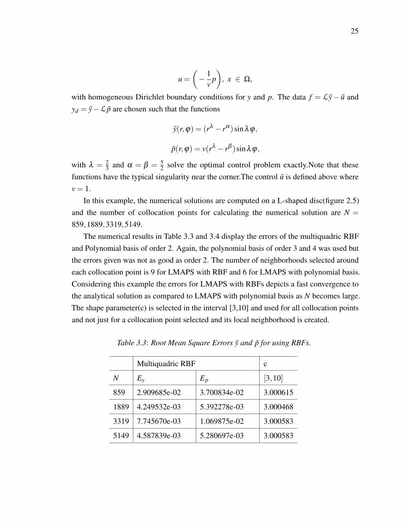
In this example, the numerical solutions are computed on a L-shaped disc(figure 2.5)and the number of collocation points for calculating the numerical solution are N =

859,1889,3319,5149.The numerical results in Table 3.3 and 3.4 display the errors of the multiquadric RBF

and Polynomial basis of order 2. Again, the polynomial basis of order 3 and 4 was used butthe errors given was not as good as order 2. The number of neighborhoods selected aroundeach collocation point is 9 for LMAPS with RBF and 6 for LMAPS with polynomial basis.Considering this example the errors for LMAPS with RBFs depicts a fast convergence tothe analytical solution as compared to LMAPS with polynomial basis as N becomes large.The shape parameter(c) is selected in the interval [3,10] and used for all collocation pointsand not just for a collocation point selected and its local neighborhood is created.

Table 3.3: Root Mean Square Errors y and p for using RBFs.

Multiquadric RBF c

N Ey Ep [3,10]

859 2.909685e-02 3.700834e-02 3.000615

1889 4.249532e-03 5.392278e-03 3.000468

3319 7.745670e-03 1.069875e-02 3.000583

5149 4.587839e-03 5.280697e-03 3.000583

26

Table 3.4: Root Mean Square Errors y and p for using Polynomial Basis.

Polynomial basis Polynomial order=2

N Ey Ep

859 7.263737e-01 6.099878e-01

1889 5.783176e-01 4.731535e-01

3319 4.994133e-01 6.651886e-01

5149 5.585314e-01 4.653635e-01

Figure 3.2: RMSE errors of y and p of LMAPS with both RBFs and Polynomial basis.

27

Chapter 4

CONCLUSIONS AND REMARKS

In this study we introduced MAPS and LMAPS for solving OCPs. On the basis of thenumerical results obtained from chapter 2 and chapter 3 examples, we have come to thefollowing conclusions and remarks:

• This is the first time MAPS and LMAPS is used to solve OCPs governed by PDEs.

• From the numerical results, we found that MAPS and LMAPS using RBFs works forOCPs governed by PDEs.

• It was also found that MAPS with polynomial basis and RBFs also works for smoothproblems.

• From the study, it was also observed that further study is needed on LMAPS andMAPS using polynomial basis to solve OCPs governed by PDEs with singularities.

• In the future, I will consider the following:

– Solving OCPs with other boundary conditions since we considered just Dirichletboundary in this study.

– Higher orders of differential equations.

– The choice of the shape parameter.

28

BIBLIOGRAPHY

[1] A.Nikoobin and M.Moradi. Indirect solution of optimal control problems with state variableinequality constraints:finite difference approximation. Robotica, pages 50–72, 35(1)(2017).

[2] C.K.Lee, X.Liu, and S.C.Fan. Local multiquadric approximation for solving boundary valueproblems. pages 396–409, 2003.

[3] C.S.Chen, A.Karageorghis, and Y.Li. On choosing the location of the sources in the mfs.Numer.Algorithms, pages 107–130, 72(2016).

[4] C.S.Chen, C.M.Fan, and P.H.Wen. The method of particular solutions for solving certainpartial differential equations. Numer.Methods Partial Differential Equations, pages 506–522,28(2012).

[5] H.Antil, M.Heinkenschloss, R.HoppeDanny, and C.Sorensen. Domain decomposition andmodel reduction for the numerical solution of pde constrained optimization problems withlocalized optimization variables. Comput. Visua. Sci, pages 249–264, 13(6)(2010).

[6] H.Antil, R.H.Nichetto, and P. Venegas. Controlling the kelvin force: basic strategies andapplications to magnetic drug targeting. Optim. Engin., pages 559–589, 19(6)(2018).

[7] H.B.Guan and D.Y.Shi. An efficient nfem for optimal control problems governed by a bilinearstate equation. Comput. Math. Appl., pages 1821–1827, 77(1)(2019).

[8] H.Guan, Y.Wang, and H.Zhu. Meshless methods for solving dirichlet boundary optimal controlproblems governed by pdes. Submitted.

[9] J.Oh, H.Zhu, and Z.Fu. An adaptive method of fundamental solutions for solving the laplaceequation. Computer and Mathematics with Applications, pages 1829–1830, 2018.

[10] Hem Raj Joshi. Optimal Control Problems in ODE and PDE Systems. PhD thesis, Universityof Tennessee-Knoxville.

[11] J.W.Pearson. A radial basis function method for solving pde-constrained optimization problems.2012.

[12] K.Eppler and F.Tröltzch. Fast optimization methods in the selective cooling of steel,OnlineOptimization of Large Scale System,pp.185-204. Springer-Verlag,Berlin„ 2001.

[13] J.L. Lions. Optimal Control of Systems Governed by Partial Differential Equations. Springer-Verlag,New York, 1971.

[14] L.S.Pontryagin, V.G.Boltyanskii, R.V.Gamkrelidze, and E.F.Mishchenko. The MathematicalTheory of Optimal Processes,Vol 4. Gordon and Breach Science Publishers, 1896.

[15] M.Darehmiraki. Reproducing kernel method for pde constrained optimization. pages 1–5,2016.

29

[16] M.I.Kamien and N.L.Schwarz. Dynamic Optimization. North-Holland,Amsterdam, 1991.

[17] Amy M.Kern. Localized meshless methods with radial basis functions for eigenvalue problems.

[18] T. Rees. Preconditioning iterative methods for PDE-constrained optimization. PhD thesis,University of Oxford.

[19] R.Y.Chang and S.Y.Yang. Solution of two-point boundary value problems by generalizedorthogonal polynomials and application to control of lumped and distributed parameter systems.Internatinal Journal of Control, pages 1785–1802, 1986.

[20] S.Rippa. An algorithm for selecting a good value for the parameter c in radial basis functionsinterpolation. Adv.Comput.Math, pages 193–210, 11(1999).

[21] T.Apel, A.Rösch, and G.Winkler. Optimal control in non-convex domains: a priori discretizationerror estimates. Numer.Algorithms, pages 138–156, 158(2007).

[22] T.R.Dangal. Numerical Solution of Partial Differential Equations Using Polynomial ParticularSolutions. PhD thesis, University of Southern Mississippi.

[23] Fredi Tröltzch. Optimal Control of Partial Differential Equations Theory, Methods and Appli-cations. Friedr, 2010.

[24] W.Gong and N.N.Yan. Mixed finite element method for dirichlet boundary control problemgoverned by elliptic pdes. SIAM J. Contr. Optim., pages 984–1014, 49(3)(2011).

[25] W.Gong, W.B.Liu, Z.Y.Tan, and N.N.Yan. A convergent adaptive finite element method for ellip-tic dirichlet boundary control problems. IMA J. Numer. Anal,Doi.org/10.1093/imanum/dry072,2018.

[26] X.Li and J.Yong. Optimal Control Theory for Infinite Dimensional Systems. Birkhäuser, 1995.

[27] Guangming Yao. Local Radial Basis Function Methods For Solving Partial DifferentialEquations. PhD thesis, University of Southern Mississippi.

[28] Dong Yichuan. Adaptive method of approximate particular solution for one-dimensionaldifferential equations. Master’s thesis, University of Southern Mississippi.