An invitation to quantum tomography

arX

iv:m

ath/

0405

595v

2 [m

ath.

ST

] 1

Jun

2004 An invitation to quantum tomography

L.M. Artiles

Eurandom, P.O. Box 513, 5600 MB Eindhoven, The Netherlands, [email protected],http://euridice.tue.nl/∼lartiles/

R. Gill

Mathematical Institute, University of Utrecht, Box 80010, 3508 TA Utrecht, The Netherlands,[email protected], http://www.math.uu.nl/people/gill

M.I. Guta

Eurandom, P.O. Box 513, 5600 MB Eindhoven, The Netherlands, [email protected],http://euridice.tue.nl/∼mguta/

Summary. The quantum state of a light beam can be represented as an infinite dimensionaldensity matrix or equivalently as a density on the plane called the Wigner function. We de-scribe quantum tomography as an inverse statistical problem in which the state is the unknownparameter and the data is given by results of measurements performed on identical quantumsystems. We present consistency results for Pattern Function Projection Estimators as well asfor Sieve Maximum Likelihood Estimators for both the density matrix of the quantum state andits Wigner function. Finally we illustrate via simulated data the performance of the estimators.An EM algorithm is proposed for practical implementation. There remain many open problems,e.g. rates of convergence, adaptation, studying other estimators, etc., and a main purpose ofthe paper is to bring these to the attention of the statistical community.

1. Introduction

It took more than eighty years from its discovery till it was possible to experimentally determine andvisualize the most fundamental object in quantum mechanics, the wave function. The forward routefrom quantum state to probability distribution of measurement results has been the basic stuff ofquantum mechanics textbooks for decennia. That the corresponding mathematical inverse problemhad a solution, provided (speaking metaphorically) that the quantum state has been probed from asufficiently rich set of directions, had also been known for many years. However it was only withSmithey et al. (1993), that it became feasible to actually carry out the corresponding measurementson one particular quantum system—in that case, the state of one mode of electromagnetic radiation(a pulse of laser light at a given frequency). Experimentalists have used the technique to establishthat they have succeeded in creating non-classical forms oflaser light such as squeezed light andSchrodinger cats. The experimental technique we are referring to here is called quantum homodynetomography: the word homodyne referring to a comparison between the light being measured witha reference light beam at the same frequency. We will explainthe word tomography in a moment.

The quantum state can be represented mathematically in manydifferent but equivalent ways, allof them linear transformations on one another. One favoriteis as the Wigner functionW: a realfunction of two variables, integrating to plus one over the whole plane, but not necessarily nonneg-ative. It can be thought of as a “generalized joint probability density” of the electric and magnetic

†Key words and phrases. Quantum tomography, Wigner function, Density matrix, Pattern Functions estima-tion, Sieve Maximum Likelihood estimation, E.M. algorithm.

http://arXiv.org/abs/math/0405595v2

2 L.M. Artiles et al.

fields,q andp. However one cannot measure both fields at the same time and inquantum mechan-ics it makes no sense to talk about the values of both electricand magnetic fields simultaneously.It does, however, make sense to talk about the value of any linear combination of the two fields,say cos(φ)q+ sin(φ)p. And one way to think about the statistical problem is as follows: the un-known parameter is a joint probability densityW of two variablesQ andP. The data consists ofindependent samples from the distribution of(X,Φ) = (cos(Φ)Q+sin(Φ)P,Φ), whereΦ is chosenindependently of(Q,P), and uniformly in the interval[0,π]. Write down the mathematical modelexpressing the joint density of(X,Φ) in terms of that of(Q,P). Now just allow that latter jointdensity,W, to take negative as well as positive values (subject to certain restrictions which we willmention later). And that is the statistical problem of this paper.

This is indeed a classical tomography problem: we take observations from all possible one-dimensional projections of a two-dimensional density. Thenon-classical feature is that though allthese one-dimensional projections are indeed bona-fide probability densities, the underlying two-dimensional “joint density” need not itself be a bona-fide joint probability density, but can havesmall patches of “negative probability”.

Though the parameter to be estimated may look strange from some points of view, it is math-ematically very nice from others. For instance, one can alsorepresent it by a matrix of (a kindof) Fourier coefficients: one speaks then of the “density matrix” ρ. This is an infinite dimensionalmatrix of complex numbers, but it is a positive and selfadjoint matrix with trace one. The diago-nal elements are real numbers summing up to one, and forming the probability distribution of thenumber of photons found in the light beam (if one could do thatmeasurement). Conversely, anysuch matrixρ corresponds to a physically possible Wigner functionW, so we have here a con-cise mathematical characterization of precisely which “generalized joint probability densities” canoccur.

The initial reconstructions were done by borrowing analytic techniques from classical tomog-raphy – the data was binned and smoothed, the inverse Radon transform carried out, followed bysome Fourier transformations. At each of a number of steps, there are numerical discretization andtruncation errors. The histogram of the data will not lie in the range of the forward transformation(from quantum state to density of the data). Thus the result of blindly applying an inverse will notbe a bona-fide Wigner function or density matrix. Moreover the various numerical approximationsall involve arbitrary choices of smoothing, binning or truncation parameters. Consequently the finalpicture can look just how the experimenter would like it to look and there is no way to statisticallyevaluate the reliability of the result. On the other hand thevarious numerical approximations tendto destroy the interesting “quantum” features the experimenter is looking for, so this method lost inpopularity after the initial enthousiasm.

So far there has been little attention paid to this problem bystatisticians, although on the onehand it is an important statistical problem coming up in modern physics, and on the other hand it is“just” a classical nonparametric statistical inverse problem. The unknown parameter is some objectρ, or if you preferW, lying in an infinite dimensional linear space (the space of density matrices, orthe space of Wigner functions; these are just two concrete representations in which the experimenterhas particular interest). The data has a probability distribution which is a linear transform of theparameter. Considered as an analytical problem, we have an ill-posed inverse problem, but onewhich has a lot of beautiful mathematical structure and about which a lot is known (for instance,close connection to the Radon transform). Moreover it has features in common with nonparametricmissing data problems (the projections from bivariate to univariate, for instance, and there are moreconnections we will mention later) and with nonparametric density and regression estimation. Thuswe think that the time is ripe for this problem to be “cracked”by mathematical and computationalstatisticians. In this paper we will present some first stepsin that direction.

An invitation to quantum tomography 3

Our main theoretical results are consistency theorems for two estimators. Both estimators arebased on approximating the infinite dimensional parameterρ by a finite dimensional parameter,in fact, thinking ofρ as an infinite dimensional matrix, we simply truncate it to anN×N matrixwhere the truncation levelN will be allowed to grow with the number of observationsn. The firstestimator employs some analytical inverse formulas expressing the elements ofρ as mean values ofcertain functions, called pattern functions, of the observations(X,Φ). Simply replace the theoreticalmeans by empirical averages and one has unbiased estimatorsof the elements ofρ, with moreoverfinite variance. If one applies this technique without truncation the estimate of the matrixρ as awhole will typically not satisfy the nonnegativity constraints. The resulting estimator will not beconsistent either, with respect to natural distance measures. But provided the truncation level growswith n slowly enough, the overall estimator will be consistent. The effect of truncating the densitymatrixρ is to project on the subspace generated by the first elements of the corresponding basis, weshall call it the Pattern Function Projection estimator (PFP).

The second estimator we study is sieve maximum likelihood (SML) based on the same trun-cation to a finite dimensional problem. The truncation levelN has to depend on sample sizen inorder to balance bias and variance. We prove consistency of the SML estimator under an appropri-ate choice ofN(n) by applying a general theorem of van de Geer (2000). To verifythe conditionswe need to bound certain metric entropy integrals (with bracketing) which express the size of thestatistical model under study.

This turns out to be feasible, and indeed to have an elegant solution, by exploiting features of themapping from parameters (density matrices) to distributions of the data. Various distances betweenprobability distributions possess analogues as distancesbetween density matrices, the mapping fromparameter to data turns out to be a contraction, so we can bound metric entropies for the statisticalmodel for the data with quantum metric entropies for the class of density matrices. And the lattercan be calculated quite conveniently.

Our results form just a first attempt at studying the statistical properties of estimators which arealready being used by experimental physicists, but they show that the basic problem is both rich ininteresting features and tractable to analysis. The main results so far are consistency theorems forPFP and SML estimators, of both the density matrix and the Wigner function. These results dependon an assumption of the rate at which a truncated density matrix approximates the true one. It seemsthat the assumption is satisfied for the kinds of states whichare met with in practice. However,further work is needed here to describe in physically interpretable terms, when the estimators work.Secondly, we need to obtain rates of consistency and to further optimize the construction of theestimator. Thirdly, one should explore the properties of penalized maximum likelihood. This willmake the truncation level data driven. Fourthly, one shouldtry to make the estimators adaptivewith respect to the smoothness of the parameter. We largely restrict attention to an ideal case ofthe problem where there is no further noise in the measurements. In practice, the observations haveadded to them Gaussian disturbances of known variance. There are some indications that when thevariance is larger than a threshold of 1/2, reconstruction becomes qualitatively much more difficult.This needs to be researched from the point of view of optimal rates of convergence.

We also only considered one particular though quite convenient way of sieving the model, i.e.,one particular class of finite dimensional approximations.There are many other possibilities andsome of them might allow easier analysis and easier computation. For instance, instead of truncatingthe matrixρ in a given basis, one could truncate in an arbitrary basis, sothat the finite dimensionalapproximations would correspond to specifyingN arbitrary state vectors and a probability distri-bution over these “pure states”. Now the problem has become amissing data problem, where the“full data” would assign to each observation also the label of the pure state from which it came.In the full data problem we need to reconstruct not a matrix but a set of vectors, together with an


ordinary probability distribution over the set, so the “full data” problem is statistically speaking amuch easier problem that the missing data problem. We shall use a version of this to derive anExpectation-Maximization algorithm (EM) for the practical implementation of the SML estimator,see Section 5. One could imagine that Bayesian reconstruction methods could also exploit thisstructure.

The analogy with density estimation could suggest new statistical approaches here. Finally, it ismost important to add to the estimated parameter, estimatesof its accuracy. This is absolutely vitalfor applications, but so far no valid approach is available.

In Section 2 we introduce first, very briefly, the statisticalproblems we are concerned with. Wethen give a short review of the basic notions of quantum mechanics which are needed in this paper.Concepts such as observables, states, measurements and quantum state tomography are explainedby using finite dimensional complex matrices. At the end of the section we show how to generalizethis to the infinite dimensional case and describe the experimental set-up of Quantum HomodyneDetection pointing out the relation with computerized tomography.

In Section 3 we present results on consistency of density matrix estimators: projection estimatorbased on pattern functions, and sieve maximum likelihood estimator. The last subsection extendsthe results of the previous ones to estimating the Wigner function.

Section 4 deals with the detection losses occurring in experiments due in part to the inefficiencyof the detectors. This adds a deconvolution problem on the top of our tomography estimation.

Section 5 shows experimental results. We illustrate the behavior of the studied estimators andpropose some practical tools for the implementation — EM algorithm. The last section finishes withsome concluding remarks to the whole paper and open problems. The main purpose of the paperis to bring the attention of the statistical community to these problem; thus, some proofs are justsketched. They fully appear in a complementary paper, Gut˘a (2004).

2. Physical background

Our statistical problem is to reconstruct the quantum stateof light by using data obtained from mea-suring identical pulses of light through a technique calledQuantum Homodyne Detection (QHD).In particular we will estimate the quantum state in two different representations or parameteriza-tions: the density matrix and the Wigner function. The physics behind this statistical problem ispresented in subsection 2.2 which serves as introduction tobasic notions of quantum theory, andsubsection 2.3 which describes the model of quantum homodyne detection from quantum optics.The relations between the different parameters of the problem are summarized in the diagram at theend of subsection 2.3 followed by Table 1 containing some examples of quantum states. For thereader who is not interested in the quantum physics background we state the statistical problem inthe next subsection and we will return to it in Section 3.

2.1. Summary of statistical problemWe observe(X1,Φ1), . . . ,(Xn,Φn), i.i.d. random variables with values inR× [0,π] and distributionPρ depending on the unknown parameterρ which is an infinite dimensional matrixρ = [ρ j ,k] j ,k=0,...,∞such that Trρ = 1 (trace one) andρ ≥ 0 (positive definite). The probability density ofPρ is

pρ(x,φ) =1π

∞

∑j ,k=0

ρ j ,kψk(x)ψ j (x)e−i( j−k)φ, (1)

where the functions{ψn} to be specified later, form a orthonormal basis of the space ofcomplexsquare integrable functions onR. Becauseρ is positive definite and has trace 1, this is a probability


density: real, nonnegative, integrates to 1. The data(Xℓ,Φℓ) comes from independent QHD mea-surements on identically prepared pulses of light whose properties or state are completely encodedin the matrixρ called a density matrix. We will consider the problem of estimatingρ from a givensample.

Previous attempts by physicists to estimate the density matrix ρ have focused mainly on theestimation of the individual matrix elements without considering the accuracy of the estimated den-sity matrix with respect to natural distances of the underlying parameter space. In Section 3 wewill present consistency results in the space of density matrices w.r.t. L1 andL2-norms using twodifferent types of estimators, namely projection and sievemaximum likelihood estimators.

An alternative representation of the quantum state is through the Wigner functionWρ : R2 → R

whose estimation is close to a classical computer tomography problem namely, Positron EmissionTomography (PET), Vardi et al. (1985). In PET one would like to estimate a probability densityfon R2 from i.i.d. observations(X1,Φ1), . . . ,(Xn,Φn), with probability density equal to the Radontransform off :

R [ f ](x,φ) =∫ ∞

−∞f (xcosφ+ t sinφ,xsinφ− t cosφ)dt.

Although the Wigner function is in generalnotpositive, its Radon transform is always a probabilitydensity, in factR [Wρ](x,φ) = pρ(x,φ). As the Wigner functionWρ is in one-to-one correspondencewith the density matrixρ, our state reconstruction problem can be stated as to estimate the WignerfunctionWρ. This is an ill posed inverse problem as seen from the formulafor the inverse of theRadon transform

Wρ(q, p) =1

2π2

∫ π

0

∫ +∞

−∞pρ(x,φ)K(qcosφ+ psinφ−x)dxdφ, (2)

where

K(x) =12

∫ +∞

−∞|ξ|exp(iξx)dξ, (3)

makes sense only as a generalized function. To correct this one usually makes a cut-off in the rangeof the above integral and gets a well behaved kernel functionKc(x) = 1

2

∫ c−c |ξ|exp(iξx)dξ. Then the

tomographic estimator ofWρ is the average sampled kernel

Wc,n(q, p) =1

2π2n

n

∑ℓ=1

Kc(qcosΦℓ + psinΦℓ −Xℓ).

For consistency one needs to let the ‘bandwidth’h = 1/c depend on the sample sizen andhn → 0asn→ ∞ at an appropriate rate.

In this paper we will not follow this approach, which will be treated separately in future work.Instead, we use a plug-in type estimator based on the property

Wρ(q, p) =∞

∑k, j=0

ρk, jWk, j(q, p), (4)

whereWk, j ’s are known functions and we replaceρ by its above mentioned estimators. We shallprove consistency of the proposed estimators of the Wigner function w. r. t.L2 and supremum normsin the corresponding space.


2.2. Quantum systems and measurementsThis subsection serves as a short introduction to the basic notions of quantum mechanics which willbe needed in this paper. For simplicity we will deal first withfinite dimensional quantum systemsand leave the infinite dimensional case for the next subsection. For further details on quantumstatistical inference we refer to the review Barndorff-Nielsen et al. (2003) and the classic textbooksHelstrom (1976) and Holevo (1982).

In classical mechanics the state of macroscopic systems like billiard balls, pendulums or stellarsystems is described by points on a manifold or “phase space”, each of the point’s coordinatescorresponding to an attribute which we can measure such as position and momentum. Therefore thefunctions on the phase space are called observables. When there exists uncertainty about the exactpoint in the phase space, or we deal with a statistical ensemble, the state is modelled by a probabilitydistribution on the phase space, and the observables becomerandom variables.

Quantum mechanics also deals with observables such as position and momentum of a particle,spin of an electron, number of photons in a cavity, but breaksfrom classical mechanics in thatthese are no longer represented by functions on a phase spacebut by Hermitian matrices, that is,complex valued matrices which are invariant under transposition followed by complex conjugation.For example, the components in different directions of the spin of an electron are certain 2× 2complex Hermitian matricesσx,σy,σz.

Any d-dimensional complex Hermitian matrixX can be diagonalized by changing the standardbasis ofCd to another orthonormal basis{e1, . . . ,ed} such thatXei = xiei for i = 1, . . . ,d, withxi ∈ R. The vectorsei and numbersxi are called eigenvectors and respectively eigenvalues ofX.With respect to the new basis we can write

X =

x1 0 0 . . . 00 x2 0 . . . 00 0 x3 . . . 0

...0 0 0 . . . xd

The physical interpretation of the eigenvalues is that whenmeasuring the observableX we obtain(randomly) one of the valuesxi according to a probability distribution depending on the state of thesystem before measurement and on the observableX. This probability measure is degenerate if andonly if the system before measurement was prepared in a special state called an eigenstate ofX. Werepresent such a state mathematically by the projectionPi onto the one dimensional space generatedby the vectorei in C

d. Given a probability distribution{p1, . . . , pd} over the finite set{x1, . . . ,xd},we describe a statistical ensemble in which a proportionpi of systems is prepared in the statePi bythe convex combinationρ = ∑i piPi . The expected value of the random resultX when measuringthe observableX for this particular state is equal to∑i pixi which can be written shortly

Eρ(X) := Tr(ρX). (5)

Similarly, the probability distribution can be recovered as

pi = Tr(ρPi) (6)

thanks to the orthogonality property Tr(PiP j) = δi j .Now, let Y be a different observable and suppose thatY does not commute withX, that is

XY 6= YX, then the two observables cannot be diagonalized in the samebasis, their eigenvectorsare different. Consequently, states which are mixtures of eigenvectors ofX typically will not be


mixtures of eigenvectors ofY and vice-versa. This leads to an expanded formulation of thenotionof state in quantum mechanics independent of any basis associated to a particular observable, andthe recipe for calculating expectations and distributionsof measurement results.

Any preparation procedure results in an statistical ensemble, or state, which is described math-ematically by a matrixρ with the following properties

(a) ρ ≥ 0 (positive definite matrix),(b) Tr(ρ) = 1 (normalization).

In physicsρ is called adensity matrix, and is for a quantum mechanical system an analogue of aprobability density. Notice that the special state∑i piPi defined above is a particular case of densitymatrix, since it is a mixture of eigenstates of the observable X. The density matrices of dimensiond form a convex setSd, whose extremals are thepureor vectorstates, represented by orthogonalprojectionsP(ψ) onto one dimensional spaces spanned byarbitrary vectorsψ ∈ Cd. Any statecan be represented as a mixture of pure states which are not necessarily eigenstates of a particularobservable.

When measuring an observable, for exampleX, of a quantum system prepared in the stateρwe obtain a random resultX ∈ {x1, . . . ,xd} with probability distribution given by equation (6),expectation as in equation (5), and characteristic function

G(t) := Eρ(

exp(itX))

= Tr(ρexp(itX)

). (7)

In order to avoid confusion we stress the important difference betweenX which is a matrix andXwhich is a real-valued random variable. More concretely, ifwe writeρ in the basis of eigenvectors

of X then we obtain the mapM from states to probability distributionsP(X)ρ over results{x1, . . . ,xd}

M : ρ =

ρ11 ρ12 . . . ρ1d

ρ21 ρ22 . . . ρ2d. . .

ρd1 ρd2 . . . ρdd

7−→ P(X)

ρ =

ρ11

ρ22...

ρdd

.

Notice thatP(X)ρ is indeed a probability distribution as a consequence of thedefining properties

of states, and it does not contain information about the off-diagonal elements ofρ, meaning thatmeasuring only the observableX is not enough to identify the unknown state. Roughly speaking,as dim(Sd) = d2 − 1 = (d− 1)(d + 1), one has to measure on many identical systems each oneof a number ofd + 1 mutually non-commuting observables in order to have a one-to-one mapbetween states and probability distributions of results. The probing of identically prepared quantumsystems from different ‘angles’ in order to reconstruct their state is broadly namedquantum statetomographyin the physics literature.

Let us suppose that we have at our disposaln systems identically prepared in an unknown stateρ∈ Sd, and for each of the systems we can measure one of the fixed observablesX(1), . . . ,X(d+1).We write the observables in diagonal form

X(i) =d

∑a=1

xi,aPi,a (8)

wherexi,a eigenvalues andPi,a eigenstates. We will perform a randomized experiment, i.e.for eachsystem we will choose the observable to be measured by randomly selecting its index according to


a probability distributionP over{1, . . . ,d +1}. The results of the measurement on thekth systemare the pairYk = (Xk,Φk) whereΦ1, . . . ,Φn are i.i.d. with probability distributionP(Φ) andXk is theresult of measuring the observableX(Φk) whose conditional distribution is given by

PM(Xk = xi,a|Φk = i) = Tr(ρPi,a) (9)

The statistical problem is now to estimate the parameterρ from the dataY1,Y2, . . . ,Yn. In the nextsubsection we will describe quantum homodyne tomography asan analogue of this problem forinfinite dimensional systems.

2.3. Quantum homodyne tomographyAlthough correct and sufficient when describing certain quantum properties such as the spin of aparticle, the model presented above needs to be enlarged in order to cope with quantum systemswith ‘continuous variables’ which will be central in our statistical problem. This technical pointcan be summarized as follows: we replaceC

d by an infinite dimensional complex Hilbert spaceH , the Hermitian matrices becomingselfadjoint operatorsacting onH . The spectral theorem tellsus that selfadjoint operators can be ‘diagonalized’ in the spirit of (2.2) but the spectrum (the set of‘eigenvalues’) can have a more complicated structure, for example it can be continuous as we willsee below. The density matrices arepositiveselfadjoint operatorsρ such that Tr(ρ) = 1 and can beregarded as infinite dimensional matrices with elementsρk, j :=

⟨ψ j ,ρψk

⟩for a given orthonormal

basis{ψ1,ψ2, . . .} in H .The central example of a system with continuous variables inthis paper is the quantum particle.

Its basic observables position and momentum, are two unbounded selfadjoint operatorsQ andPrespectively, acting onL2(R), the space of square integrable complex valued functions onR

(Qψ1)(x) = xψ1(x),

(Pψ2)(x) = −idψ2(x)

dx,

for ψ1,ψ2 arbitrary functions. The operators satisfy Heisenberg’scommutation relationsQP−PQ = i1 which implies that they cannot be measured simultaneously.The problem of (separately)measuring such observables has been elusive until ten yearsago when pioneering experiments inquantum optics by Smithey et al. (1993), led to a powerful measurement technique calledquantumhomodyne detection. This technique is the basis of a continuous analogue of the measurementscheme presented at the end of the previous subsection whered+1 observables were measured inthe case of ad-dimensional quantum system.

The quantum system to be measured is a beam of light with a fixedfrequency whose observablesare the electric and magnetic field amplitudes which satisfycommutation relations identical to thosecharacterizing the quantum particle, with which they will be identified from now on. Their linearcombinationsXφ = cosφQ +sinφP are calledquadratures, and homodyne detection is about mea-suring the quadratures forall phasesφ ∈ [0,π]. The experimental setup shown in Figure 1 containsan additional laser called a local oscillator (LO) of high intensity|z| ≫ 1 and relative phaseφ withrespect to the beam in the unknown stateρ. The two beams are combined through a fifty-fifty beamsplitter, and the two emerging beams are then measured by twophoton detectors. A simple quantumoptics computation (see Leonhardt (1997)) shows that in thelimit of big LO intensity the differenceof the measurement results (countings) of the two detectorsrescaled by the LO intensityX = I1−I2

|z|has the probability distribution corresponding to the measurement of the quadratureXφ. The result


Fig. 1. Quantum Homodyne Tomography measurement system

X takes values inR and its probability distributionPρ(·|φ) has a densitypρ(x|φ) and characteristicfunction (see equation (7))

Gρ,Xφ(t) = Tr(ρexp(itXφ)

). (10)

The phaseφ can be controlled by the experimenter by adjusting a parameter of the local oscillator.We assume that he chooses it randomly uniformly distributedover the interval[0,π]. Then the jointprobability distributionPρ for the pair consisting in measurement result and phaseY := (X,Φ) hasdensitypρ(x,φ) equal to1

π pρ(x|φ) with respect to the measuredx×dφ on R× [0,π]. An attractivefeature of the homodyne detection scheme is the invertibility of the mapT that associatesPρ to ρ,making it possible to asymptotically infer the unknown parameterρ from the i.i.d. resultsY1, . . . ,Yn

of homodyne measurements onn systems prepared in the stateρ.We will see now why this state estimation method is calledquantum homodyne tomography

by drawing a parallel with computerized tomography used in the hospitals. In quantum opticsit is common to represent the state of a quantum system by a certain function onR2 called theWigner function Wρ(q, p) which is much like a joint probability density forQ andP, for instance itsmarginals are the probability densities for measuringQ and respectivelyP. The Wigner function ofthe stateρ is defined by demanding that its Fourier transformF2 with respect tobothvariables hasthe following property

Wρ(u,v) := F2[Wρ](u,v) = Tr(ρexp(−iuQ− ivP)

). (11)

We see from this equation that ifQ andP were commuting operators thenW(q, p) would indeed bethe joint probability density of outcomes of their measurement. As the two observables cannot bemeasured simultaneously, we cannot speak of a joint density, in fact the Wigner function need notbe positive, but many interesting features of the quantum state can be visualized in this way. Let(u,v) = (t cosφ, t sinφ), then

W(u,v) = F1[p(·,φ)](t) = Tr(ρexp(−itXφ)

)(12)

where the Fourier transformF1 in the last term is with respect to the first variable, keepingφ fixed.


The equations (11) and (12) are well known in the theory of Radon transformR and imply thatfor each fixedφ, the probability densitypρ(x,φ) is the marginal of the Wigner function with respectto the directionφ in the plane,

pρ(x,φ) = R [Wρ](x,φ) =∫ ∞

−∞Wρ(xcosφ+ysinφ,xsinφ−ycosφ)dy, (13)

adding quantum homodyne tomography to a number of applications ranging from computerizedtomography to astronomy and geophysics, Deans (1983). In computerized tomography one recon-structs an image of the tissue distribution in a cross-section of the human body by recording eventswhereby pairs of positrons emitted by an injected radioactive substance hit detectors placed in a ringaround the body after flying in opposite directions along an axis determined by an angleφ ∈ [0,π].In quantum homodyne tomography the role of the unknown distribution is played by the Wignerfunction which is in general not positive, but has a probability density pρ(x|φ) as marginal alongany directionφ.

The following diagram summarizes the relations between thevarious objects in our problem:

ρ Wρ pρ(x,φ) (X1,Φ1), . . . ,(Xn,Φn).

Wρ

..................................................................................................

............

..................................................................................................

............

....................................................................................................................................................................................

............

R

.

..

.

..

.

..

.

..

.

..

.

..

.

..

.

..

.

..

.

..

.

..

.

..

.

.

..

.

..

.

..

.

..

.

..

.

..

.

..

.

..

.

..

.

..

.

..

.

..

.

.

..

.

..

.

..

.

..

.

..

.

..

.

..

.

..

.

..

.

..

.

..

.

.

..

.

..

.

..

.

..

.

..

.

..........

.

.

.

.

.

.

.

.

.

.

.

.

F2

.

..

.

..

.

..

.

..

.

..

..

.

..

.

..

.

..

.

..

.

..

.

..

..

.

..

.

..

.

..

.

..

.

..

..

.

..

.

..

.

..

.

..

.

..

..

.

..

.

..

.

..

.

..

.

..

.

..........................................

.

...........

F1

......................................................................................................................................................

............

experiment

Finally in Table 1 we give some examples of density matrices and their corresponding Wignerfunction representations for different states. The matrixelementsρk, j are calculated with respect tothe orthonormal base corresponding to the wave functions ofk photons states

ψk(x) = Hk(x)e−x2/2 (14)

whereHk are the Hermite polynomials normalized such that∫

ψ2k = 1. A few graphical representa-

tions can be seen in Figure 3.

State Density matrixρk, j Wigner functionW(q, p)

Vacuum state ρ0,0 = 1, rest zero 1π exp(−q2− p2)

Single Photon state ρ1,1 = 1, rest zero 1π(2q2 +2p2−1)exp(−q2− p2)

Thermal stateβ > 0 δ jk(1−e−β)e−βk 1

π tanh(β/2)exp[−(q2+ p2) tanh(β/2)]

Coherent state,N ∈ R+ exp(−N) Nk+ j√k! j !

1π exp(−(q−

√N)2− p2)

Squeezed state C(N,ξ)(12 tanh(ξ))k+ j× 1

π exp(−e2ξ(q−α)2−e−2ξp2)

N ∈ R+ , ξ ∈ R, H j(γ)Hk(γ)/√

j!k!

Table 1: Density matrix and Wigner function of some quantum states

The vacuum is the pure state of zero photons, notice that in this case the distributions ofQ andP are Gaussian. The thermal state is a mixed state describing equilibrium at temperatureT = 1/β,


having Gaussian Wigner function with variance increasing with the temperature. The coherent stateis pure and characterizes the laser pulse. The photon numberis Poisson distributed with an averageof N photons. The squeezed states have Gaussian Wigner functions whose variances for the twodirections are different but have a fixed product. The parametersN and ξ satisfy the condition

N ≥ sinh2(ξ), C(N,ξ) is a normalization constant,α = (N−sinh2(ξ))1/2

cosh(ξ)−sinh(ξ), andγ = ( α

sinh(2ξ))1/2.

3. Density matrix estimation

D’Ariano et al. (1994) presented the density matrix analogue of formula (2) of the Wigner functionas inverse Radon transform of the probability densitypρ

ρ =

∫ ∞

−∞dx∫ π

0

dφπ

pρ(x,φ)K(Xφ −x1), (15)

whereK is the generalized function given in equation (3) whose argument is a selfadjoint operatorXφ − x1. The method has been further analyzed in D’Ariano (1995), Leonhardt et al. (1995), seealso D’Ariano et al. (1995). We recall that in the case of the Wigner function we needed to regularizethe kernelK by introducing a cut-off in the integral (3). For density matrices the philosophy will berather to project on a finite dimensional subspace ofL2(R) whose dimensionN will play the role ofthe cut-off. In fact all the matrix elements of the density matrix ρ with respect to the orthonormalbasis{ψk}∞

k=0 defined in (14), can be expressed as kernel integrals

ρk, j =

∫ ∞

−∞dx∫ π

0

dφπ

pρ(x,φ) fk, j (x)e−i( j−k)φ, (16)

with fk, j = f j ,k bounded real valued functions which in the quantum tomography literature arecalledpattern functions. The singularity of the kernelK is reflected in the asymptotic behavior offk, j ask, j → ∞. A first formula for fk, j was found in Leonhardt et al. (1995) and uses Laguerrepolynomials. This was followed by a more transparent one dueto Leonhardt et al. (1996),

fk, j (x) =ddx

(ψk(x)ϕ j (x)), (17)

for j ≥ k, whereψk andϕ j represent the square integrable and respectively the unbounded solutionsof the Schrodinger equation,

[−1

2d2

dx2 +12

x2]

ψ = ω ψ, ω ∈ R. (18)

Figure 2 shows pattern functions for different values ofk and j. We notice that the oscillatory partis concentrated in an interval centered at zero whose lengthincrease withk and j, the number ofoscillations increases withk and j and the functions become more irregular as we move away fromthe diagonal. It can be shown that tails of the pattern function decay likex−2−|k− j |. More propertiesof the pattern function can be found in Leonhardt et al. (1996) and Guta (2004).

3.1. Pattern function projection estimationEquation (16) suggests theunbiased estimatorρ(n) of ρ, based onn i.i.d. observations of(X,Φ),whose matrix elements are:

ρ(n)k, j =

1n

n

∑ℓ=1

Fk, j(Xℓ,Φℓ), (19)


Fig. 2. Pattern functions

whereFk, j(x,φ) = fk, j (x)e−i( j−k)φ, see D’Ariano et al. (1995), Leonhardt et al. (1995, 1996). Bythe strong law of large numbers the individual matrix elements of this estimator converge to thematrix elements of the true parameterρ. However the infinite matrixρ(n) need not be positive,normalized, or even selfadjoint, thus it cannot be interpreted as a quantum state. These problemsare similar to those encountered when trying to estimate an unknown probability density by usingunbiased estimators for all its Fourier coefficients. The remedy is to estimate only a finite number ofcoefficients at any moment, obtaining a projection estimator onto the subspace generated by linearcombinations of a finite subset of the basis vectors. In our case we will project onto the space ofmatrices of dimensionN = N(n) with respect to the basis{ψk}∞

k=0,

ρ(N,n)k, j =

1n

n

∑ℓ=1

Fk, j(Xℓ,Φℓ), for 0≤ k, j ≤ N−1,

andρ(n)k, j = 0 for (k∧ j) ≥ N.

In order to test the performance of our estimators we introduce theL1 andL2 distances on thespace of density matrices. Letρ andτ be two density matrices withρ− τ = ∑i λiPi the diagonalform of their difference, and notice that some of the eigenvalues are positive and some negative suchthat their sum is zero due to the normalization of the densitymatrices. We define the absolute value|ρ− τ| := ∑i |λi |Pi and the norms

‖ρ− τ‖1 := Tr(|ρ− τ|), (20)

‖ρ− τ‖2 :=[Tr(|ρ− τ|2)

]1/2=

[∞

∑j ,k=0

|ρk, j − τk, j |2]1/2

. (21)

Let us consider now the mean integrated square error (MISE) and split it into the bias and


variance parts:

E( ∞

∑j ,k=0

|ρ(N,n)k, j −ρk, j |2

)= ∑

(k∧ j)≥N

|ρk, j |2 +E( N−1

∑j ,k=0

|ρ(N,n)k, j −ρk, j |2

)= b2(n)+ σ2(n). (22)

By choosingN(n) → ∞ asn → ∞ the biasb2(n) converges to zero. For the variance we have theupper bound

σ2(n) =1n

N−1

∑j ,k=0

∫ π

0

∫

R

|Fk, j(x,φ)−ρk, j |2pρ(x,φ)dφdx

≤ 1n

N−1

∑j ,k=0

∫ π

0

∫

R

|Fk, j(x,φ)|2pρ(x,φ)dφdx

=1n

N−1

∑j ,k=0

∫

R

dx fk, j(x)2∫ π

0pρ(x,φ)dφ. (23)

The proof of the following lemma on the norms of the pattern functions can be found in Guta (2004).

LEMMA 3.1. There exist constants C1,C2,C3 such that

N

∑k, j≥0

‖ fk, j‖2∞ ≤C1N7/3, (24)

N

∑k, j≥0

‖ fk, j‖22 ≤C2N3, (25)

∫ 2π

0pρ(x,φ)dφ ≤C3, for all x∈ R. (26)

By applying the lemma to equation (23) we conclude that the estimator ρ(N,n) is consistent withrespect to theL2 distance if we chooseN(n) → ∞ asn→ ∞ such thatN(n) = o(n3/7). Based onthe property‖ρ(N,n)‖1 ≤

√N‖ρ(N,n)‖2 we can prove a similar result concerningL1-consistency, see

Guta (2004).

THEOREM 3.2. Let N(n) → ∞ be the dimension of the pattern function projection estimator. IfN(n) = o(n3/7), then

E(‖ρ(N,n)−ρ‖2

2

)→ 0, asn→ ∞. (27)

If N(n) = o(n3/10) then

E(‖ρ(N,n)−ρ‖1

)→ 0, asn→ ∞. (28)

Rates of consistency can be obtained by assuming that the state belongs to a given class for whichupper bounds of the bias can be calculated andN(n) is chosen such as to balance bias and variance.This problem will be attacked in future work within the minimax framework. In Section 5 wepresent a data-dependent way of selecting the dimension of the projection estimator based on theminimization of the empiricalL2-risk using a cross-validation technique.


3.2. Sieve maximum likelihood estimationWe will consider now a maximum likelihood approach to the estimation of the stateρ. Let usrecall the terms of the problem: we are given a sequenceY1,Y2 . . . ,Yn of i.i.d. random variablesYi = (Xi ,Φi) with values inR× [0,π] and probability densitypρ depending on the parameterρwhich is an infinite dimensional density matrix. We would like to find an estimator ofρ

ρ(n) = ρ(n)(Y1,Y2, . . . ,Yn).

Let ρ andτ be density matrices and denote by

h(Pρ,Pτ) :=

(∫(√

pρ −√

pτ)2 dxdϕ

)1/2

, (29)

the Hellinger distance between the two probability distributions. The following relations are wellknown

dtv(Pρ,Pτ) =12‖pρ − pτ‖1 ≤ h(Pρ,Pτ) ≤

√‖pρ − pτ‖1, (30)

An important property which is true for any measurement is the following inequality between theclassical and quantum distances, cf. Guta (2004),

‖pρ − pτ‖1 ≤ ‖ρ− τ‖1. (31)

From (30) and (31) we obtainh(Pρ,Pτ) ≤

√‖ρ− τ‖1, (32)

for arbitrary statesρ,τ. As we have seen previously, the inverse map fromPρ to ρ is unboundedthus we do not have an inequality in the opposite direction tothe one above. However we can provethe continuity of the inverse map by using a matrix analogue of the Scheffe’s lemma from classi-cal probability (see Williams (1991)) stating that if a sequence of probability densities convergespointwise almost everywhere to a probability density, thenthey also converge in total variationnorm. The matrix Scheffe’s lemma which can be found in Simon(1979) says that ifρ,ρ(1),ρ(2), . . .

are density matrices (positive and trace one) and if the coefficientsρ(n)i, j converge toρi, j asn goes

to infinity, for any fixed indicesi, j, then‖ρ(n) − ρ‖1 → 0. But by equation (16) if the sequence

Pρ(n) converges toPρ asn→ ∞ with respect to thedtv-distance thenρ(n)i, j converges toρi, j and thus

‖ρ(n)−ρ‖1 → 0, completing the proof of the continuity of the map fromPρ to ρ. In particular wehave‖ρ(n)−ρ‖2 → 0 due to the inequality between theL1 andL2 norms

‖τ−ρ‖2 ≤ ‖τ−ρ‖1. (33)

The maximum likelihood estimator ofρ is defined as

argmaxτ

n

∑ℓ=1

logpτ(Xℓ,Φℓ) (34)

where the maximum is taken over all density matrices in on thespaceL2(R). However there existdensity matricesτ such that the probability densitypτ takes arbitrarily high values at all the points(Xℓ,Φℓ). To see this let us first remind the reader that any density matrix is a convex combinationof “pure states” which are projectionsP(ψ) on one dimensional sub-spaces ofL2(R) generated byvectorsψ which can be written as a Fourier sum

ψ(x) =∞

∑k=0

αkψk(x) (35)


in the basis{ψk} given in equation (14), with∫ |ψ(x)|2dx= ∑k |αk|2 = 1. For any such state the

corresponding probability density is

pψ(x,φ) =∣∣∣

∞

∑k=0

αkeikφψk(x)

∣∣∣2= |ψφ|2(x), (36)

whereψφ(x) is the square integrable function with Fourier coefficientseikφαk. It is clear that thereexists a one-to-one relation betweenψ andψφ which preserves theL2-norms, thus we can choosevectorsϕ1, . . .ϕn such that

∫|ϕℓ(x)|2dx = 1 and |ϕΦℓ

ℓ (Xℓ)|2 > C for all ℓ = 1, . . .n and arbitraryC > 0. Then the density matrix

ρ =1n

n

∑k=1

P(ϕk) (37)

representing a statistical mixture of the pure states leadsto the likelihood

pρ(x,φ) =n

∏ℓ

(1n

n

∑k=1

|ϕΦℓk (Xℓ)|2

)≥(C

n

)n. (38)

which can be arbitrarily high for any fixedn. This drawback can be corrected by using for examplepenalized maximum likelihood estimators or by restrictingthe state space to some subspaceQ (n) ofdensity matrices such that for any amount of data the maximumof the likelihood overQ (n) existsand∪nQ (n) is dense in the space of all density matricesS with respect to some chosen distancefunction. Such a method is called sieve maximum likelihood and we refer to van de Geer (2000)and Wong and Shen (1995) for the general theory. The choice ofthe sievesQ (n) should be tailoredaccording to the problem one wants to solve, the class of states one is interested in, etc. Here wewill use the same subspaces as for the projection estimator of the previous subsection, that isQ (n)consists of those states with maximallyN(n)− 1 photons described by density matrices over thesubspace spanned by the basis vectorsψ0, . . . ,ψN(n)−1. We will call {Q (n)}n≥0 thenumber statessievesand the dimensionN(n) will be an increasing function ofn which will be fixed later so as toguarantee consistency.

Q (n) ={

τ ∈ S : τ j ,k = 0 for all j ≥ N(n) or k≥ N(n)}

. (39)

Notice that the dimension of the spaceQ (n) is N(n)2−1. Let now the estimator be

ρ(n) := arg maxτ∈Q (n)

n

∑ℓ=1

logpτ(Xℓ,Φℓ), (40)

where the maximum can be shown to exist for example by using compactness arguments. We willdenote the corresponding sieve in the space of probability densities by

P (n) = {pτ : τ ∈ Q (n)} . (41)

The theory of M-estimators van de Geer (2000) tells us that the consistency of ML estimatorsdepends essentially on the “size” of the parameter space, inour case the sievesQ (n) or P (n), whichis measured by entropy numbers with respect to some distance, for example theL1-norm on densitymatrices or the Hellinger distance between probability distributions.

DEFINITION 3.3. LetG be a class of density matrices. Let NB,1(δ,G ) be the smallest value ofp∈ N for which there exist pairs of Hermitian matrices (not necessarily density matrices)[τL

j ,τUj ]


with j = 1, . . . , p such that‖τLj − τU

j ‖1 ≤ δ for all j, and such that for eachτ ∈ G there is a j=j(τ) ∈ {1, . . . , p} satisfying

τLj ≤ τ ≤ τU

j .

Then HB,1(δ,G ) = logNB,1(δ,G ) is calledδ-entropy with bracketing ofG .

We note that this definition relies on the concept of positivity of matrices and the existence of theL1-distance between states. But the same notions exist for thespace of integrable functions thusby replacing density matrices with probability densities and selfadjoint operators with functionswe obtain the definition of theδ-entropy with bracketingHB,1(δ,F ) for some space of probabilitydensitiesF , see van de Geer (2000). Moreover by using equation (31) and the fact that the linearextension of the map from density matrices to probability densities sends a positive matrix to apositive function, we get that for anyδ-bracketing[τL

j ,τUj ] for Q (n), the corresponding functions

[pLj , pU

j ] form aδ-bracketing forP (n), i.e. they satisfy‖pLj − pU

j ‖1 ≤ δ and for anyp∈ P (n) there

exists aj = j(p) such thatpLj ≤ p≤ pU

j . Thus

HB,1(δ,P (n)) ≤ HB,1(δ,Q (n)).

The following proposition gives an upper bound of the “quantum” bracketing entropy and in conse-quence forHB,1(δ,P (n)). Its proof can be found in Guta (2004) and relies on choosing a maximalnumber of nonintersecting balls centered inQ (n) having radius δ

2N(n) and then providing a pair ofbrackets for each ball.

PROPOSITION3.4. LetQ (n) be the class of density matrices of dimension N(n). Then

HB,1(δ,Q (n)) ≤CN(n)2 logN(n)

δ. (42)

for some constant C independent of n andδ.

By combining the previous inequalities with equation (32) we get the following bound for the brack-eting entropy of the class of square-root densities

P 1/2(n) ={√

pρ : pρ ∈ P (n)}, (43)

with respect to theL2-distance

HB,2(δ,P 1/2(n)) ≤C2N(n)2 logN(n)

δ. (44)

We will concentrate now on the Hellinger consistency of the sieve maximum likelihood estimatorPn. We will appeal to a theorem from van de Geer (2000), which is similar to other results in theliterature on non-parametricM-estimation (see for example Wong and Shen (1995)). There aretwo competing factors which contribute to the convergence of h(Pn,Pρ). The first is related to theapproximation properties of the sieves with respect to the whole parameter space. Such a distancefrom ρ to the sieveQ (n) can take different expressions, for example in terms of theχ2-distancebetween the corresponding probability measures

τn := argminpn∈Pn

χ2(pρ, pn), (45)


where theχ2-distance between two probability distributions is given by

χ2(P1,P2) :=

{∫(dP1

dP2−1)2dP2 P1 ≪ P2,

∞ otherwise.(46)

Notice thatτn depends onn through the growth rate of the sieveN(n). The second factorinfluencing the convergence ofh(Pn,Pρ) is the size of the sieves which is expressed by the bracketingentropy. The non-parametric sieve maximum likelihood estimation theory shows that consistencyholds if there exists a sequenceδn → 0 such that the followingentropy integral inequalitiesaresatisfied for alln

JB(δn,P1/2(n)) :=

∫ δn

δ2n/c

H1/2B (u,P (n)1/2)du ∨ δn ≤

√nδ2

n/c. (47)

wherec is some universal constant, van de Geer (2000). From (44) we get

JB(δn,P1/2(n)) = O

[N(n)δn

(log

N(n)

δn

)1/2]

, (48)

which implies the following constraint forN(n) → ∞ andδn → 0 ,

N(n)

δn= O

(√n

logn

). (49)

THEOREM 3.5. Suppose that the stateρ satisfiesτn → 0. Let ρ(n) be the sieve MLE with N(n)andδn satisfying (47), then

P(h(Pn,Pρ) ≥ δn + τn) ≤ c exp(−nδ2n/c2). (50)

Proof. Details can be found in Guta (2004) based on Theorem 10.13 of van de Geer (2000).

From the physical point of view, we are interested in the convergence of the state estimatorρ(n) with respect to theL1 andL2-norms on the space of density matrices. Clearly the rates ofconvergence for such estimators are slower than those of their corresponding probability densities.As shown in the beginning of this subsection the map sending probability densitiespρ to densitymatricesρ is continuous, thus an estimatorρn taking values in the space of density matricesS isconsistent in theL1 or L2-norms if and only ifPn converges toPρ almost surely with respect to theHellinger distance.

COROLLARY 3.6. The Hellinger consistency ofPn is equivalent to the‖ · ‖1-consistency ofρ(n). In particular, if ∑nexp(−nδ2

n/c2) < ∞ and the assumptions of Theorem 3.5 hold, then we have‖ρ(n)−ρ‖1 → 0, a.s..

3.3. Wigner function estimationThe Wigner function plays an important role in quantum optics as an alternative way of representingquantum states and calculating an observable’s expectation: for any observableX there exists afunctionWX from R2 to R such that

Tr(Xρ) =

∫∫WX(q, p)Wρ(q, p)dqdp. (51)


Besides, physicists are interested in estimating the Wigner function for the purpose of identifyingfeatures which can be easier visualized than read off from the density matrix, for example a “non-classic” state may be recognized by its patches of negative Wigner function, while “squeezing” ismanifest through the oval shape of the support of the Wigner function, see Table 1 and Figure 3.As described in Subsection 2.3 the Wigner function should beseen formally as a joint density ofthe observablesQ andP which may take non-negative values, reflecting the fact thatthe two ob-servables cannot be measured simultaneously. However the Wigner function shares some commonproperties with probability densities, in particular their marginals

∫Wρ(q, p)dq and

∫Wρ(q, p)dp

are probability densities on the line. In fact this is true for the marginals in any direction which arenothing else then the densitiespρ(x,φ). On the other hand there exist probability densities whichare not Wigner functions and vice-versa, for example the latter cannot be too “peaked”:

|Wρ(q, p)| ≤ 1π, for all (q, p) ∈ R

2, ρ ∈ S . (52)

As a corollary of this uniform boundedness we get

‖Wρ −Wτ‖∞ ≤ 1π‖ρ− τ‖1. (53)

for any density matricesρ andτ. Indeed we can writeρ−τ = ρ+−ρ− whereρ+ and−ρ− representthe positive and negative part ofρ− τ. Then

‖Wρ −Wτ‖∞ = ‖Wρ+ −Wρ−‖∞ ≤ ‖Wρ+‖+‖Wρ−‖∞ ≤1π(‖ρ+‖1 +‖ρ−‖1) =

1π‖ρ− τ‖1.

Another important property is the fact that the linear span of the Wigner functions is dense inL2(R

2), the space of real valued, square integrable functions on the plane, and there is an isometry(up to a constant) between the space of Wigner functions and that of density matrices with respectto theL2-distances

‖Wρ −Wτ‖22 =:

∫∫|Wρ(q, p)−Wτ(q, p)|2dpdq=

12π

‖ ρ− τ ‖22 . (54)

In Section 2 we have described the standard estimation method employed in computerized tomog-raphy which used a regularized kernelKc with bandwidthhn = 1/c converging to zero asn→ ∞ atan appropriate rate. This type of estimators for the Wigner function will be analyzed separately infuture work in the minimax framework along the lines of Cavalier (2000). The estimators which wepropose in this subsection are of a different type, they are based on estimators forρ plugged into thefollowing linearity equation

Wρ(q, p) = ∑k, j

ρk, jWk, j(q, p),

whereWk, j are known functions corresponding to the matrix with the entry (k, j) equal to 1 and allthe rest equal to zero, see Leonhardt (1997). The isometry (54) implies that the family{Wk, j}∞

k, j=0

forms an orthogonal basis ofL2(R2). Following the same idea as in the previous section we consider

the projection estimator

W(n)(q, p) =N(n)−1

∑k, j=0

(1n

n

∑ℓ=1

Fk, j(Xℓ,Φℓ)

)Wk, j(q, p).


COROLLARY 3.7. Let N(n) be such that N(n) → ∞ and

N(n) = o(n3/7).

Then

E‖W(n)−Wρ‖22 = ‖W(n)

ρ −Wρ‖22 +O

(N(n)7/3

n

).

Proof: Apply isometry property and Theorem 3.2.

Similarly we can extend the SML estimator of the density matrix to the Wigner function. Definethe subspace

W (n) = {Wρ : ρ ∈ Q (n)},

with Q (n) as in equation (39), and define the corresponding SML estimator asW(n)

= Wρ(n) where

ρ(n) was defined in (40).

COROLLARY 3.8. Suppose thatρ satisfiesτn → 0. LetW(n)ρ be the SML estimator with N(n)

andδn satisfying (47) and∑nexp(−nδ2n/c2) < ∞. Then we have

‖W(n)−Wρ‖2 → 0

almost surely. Under the same conditions

‖W(n)−Wρ‖∞ → 0

almost surely.

Proof: Apply the inequalities (53, 54) and Corollary 3.6.

4. Noisy observations

The homodyne tomography measurement as presented up to now does not take into account variouslosses (mode mismatching, failure of detectors) in the detection process which modify the distribu-tion of results in a real measurement compared with the idealized case. Fortunately, an analysis ofsuch losses (see Leonhardt (1997)) shows that they can be quantified by a singleefficiencycoeffi-cient 0< η < 1 and the change in the observations amounts replacingXi by the noisy observations

X′i :=

√ηXi +

√(1−η)/2ξi (55)

with ξi a sequence of i.i.d. standard Gaussians which are independent of all Xj . The problem is againto estimate the parameterρ fromY′

i = (X′i ,Φi), for i = 1, . . . ,n. The efficiency-corrected probability

density is then the convolution

pρ(y,φ;η) = (π(1−η))−1/2∫ ∞

−∞p(x,φ)exp

[− η

1−η(x−η−1/2y)2

]dx. (56)

The physics of the detection process detailed in Leonhardt (1997) offers an alternative routefrom the state to the probability density of the observations Y′

i . In a first step one performs a


Bernoulli transformation B(η) on the stateρ which is a quantum equivalent of the convolution withnoise for probability densities, and obtains a new density matrix ρη. To understand the Bernoullitransformation let us consider first the diagonal elements{pk = ρk,k, k = 0,1..} and{q j = ρη

j , j , j =0,1..} which are both probability distributions overN and represent the statistics of the number ofphotons in the two states. Letbk+p

k =(k+p

k

)ηk(1−η)p be the binomial distribution. Then

q j =∞

∑k= j

bkj(η)pk (57)

which has a simple interpretation in terms of an “absorption” process by which each photon of thestateρ goes independently through a filter and is allowed to pass with probabilityη or absorbedwith probability 1−η. The formula of the Bernoulli transformation for the whole matrix is

ρηj ,k =

∞

∑p=0

[b j+p

j (η)bk+pk (η)

]1/2ρ j+p,k+p. (58)

The second step is to perform the usual quantum tomography measurement with ideal detectorson the “noisy” stateρη obtaining the resultsY′

i with densitypρ(x,φ;η). It is noteworty that thetransformationsB(η) form a semigroup, that is they can be composed asB(η1)B(η2) = B(η1η2)and the inverse ofB(η) is simply obtained by replacingη with η−1 in equation (58). Notice howeverthat if η ≤ 1/2 the power series(1−η−1)k appearing in the inverse transformation diverges, thuswe need to take special care in this range of parameters.

A third way to compute the inverse map frompρ(x,φ;η) to ρ is by using pattern functionsdepending onη which incorporate the deconvolution map frompρ(x,φ;η) to pρ(x,φ;1):

ρk, j =

∫ ∞

−∞dx∫ π

0

dφπ

pρ(x,φ;η) fk, j (x;η). (59)

Such functions are analyzed in D’Ariano (1995); D’Ariano etal. (1995) where it is argued that themethod has a fundamental limitation forη≤ 1/2 in which case the pattern functions are unbounded,while for η > 1/2 numerical calculations show that their range grows exponentially fast with bothindices j,k.

The two estimation methods considered in Section 3 can be applied to the state estimation withnoisy observations. The projection estimator has the same form as in Subsection 3.1 with a similaranalysis of the meanL2-risk taking into account the norms of the new pattern functions fk, j (x;η).The sieve maximum likelihood estimator follows the definition in Subsection 3.2 and a consistencyresult can be formulated on the lines of Corollary 3.6. We expect however that the rates of conver-gence will be dramatically slower and we will leave this analysis for a separate work.

5. Experimental results

In this section we study the performance of the Pattern Function Projection estimator and the SieveMaximum Likelihood estimator using simulated data. In Table 1 we showed some examples ofdensity matrices and Wigner functions of quantum states. InFigure 3, we display their correspond-ing graphical representation. For some of them the corresponding probability distribution can beexpressed explicitly and it is possible to simulate data. Inparticular we shall simulate data fromQHT measurements on squeezed states with efficiencyη = 1.


Fig. 3. Graphical representation of quantum states


5.1. ImplementationIn order to implement the two estimators we need to compute the basis functionsψn and the func-tionsφn, which are solutions of Schrodinger equation (18). For this, we use an appropriate set ofrecurrent equations, see Leonhardt (1997), Ch. 5. Pattern functions can then be calculated as

fk, j (x) = 2xψ j(x)φk(x)−√

2( j +1)ψ j+1(x)φk(x)−√

2(k+1)ψ j(x)φk+1(x),

for all j ≥ k, otherwisefk, j (x) = f j ,k(x) and thenFk, j(x,θ) = fk, j (x)ei(k− j)θ.On the practical side, finding the maximum of the likelihood function over a set of density

matrices is a more complicated problem due to the positivityand trace one constraints which mustbe taken into account. A solution was proposed in Banaszek etal. (1999), where the restriction onpositivity of a density matrixρ is satisfied by writing the Cholevski decomposition

ρ = T∗T (60)

whereT of upper triangularmatrices of the same dimension asρ with complex coefficients abovethe diagonal and reals on the diagonal. The normalization condition Trρ = 1 translates into‖T‖2 = 1which defines a ball in the space of upper triangular matriceswith theL2-distance. We will denoteby T (n) the set of such matrices having dimensionN(n). The sieve maximum likelihood estimatoris the solution of the following optimization problem withN = N(n)

T = argmaxT∈T (n)

n

∑ℓ=1

logpρ(Xℓ,Φℓ)

= argmaxTT (n)

n

∑ℓ=1

logN−1

∑k=1

∣∣∣k

∑m=0

Tk,mψm(Xℓ)eimΦℓ

∣∣∣2.

The numerical optimization was performed using a classicaldescendent method with con-straints. Notice that we have an optimization problem onN2−1 real variables. Given the problemof high dimensionality and computational cost we propose analternative method to the procedurementioned above. It exploits the mixing properties of our model. Any density matrix of dimen-sion N can be written as convex combination ofN purestates, i.e.ρ = ∑N−1

r=0 prρr , wherepr ≥ 0,∑r pr = 1 andρr is a one dimensional projection whose Cholevski decomposition is of the formρr = t∗r tr wheretr is the row vector of dimensionN on whichρr projects, andt∗r is the column vec-tor of the complex conjugate oftr . It should be noted that even though decomposition of our statein pure states is not unique this is not a problem given we are actually not interested in this repre-sentation but in the resulting convex combination, the state itself. Now we can state the problem asto find the maximizer of the loglikelihood

L({(Xℓ,Φℓ)}; p, t) =n

∑ℓ=1

logN−1

∑r=0

pr pρr (Xℓ,Φℓ) =n

∑ℓ=1

logN−1

∑r=0

pr

∣∣∣N(n)−1

∑m=0

tr,mψm(Xℓ)eimΦℓ

∣∣∣2,

wheretr,m represents the mth coordinate oftr . We now maximize over allβ ∈ B where

B =

{{pr , tr}N−1

r=0 : pr ≥ 0,N−1

∑r=0

pr = 1,‖tr‖2 = 1, for all r

}.

We propose an EM algorithm as an alternative method to the onepresented in Banaszek et al.(1999). See, Dempster et al. (1977) for an exposition on the formulation of the EM algorithm for


problems of ML estimation with mixtures of distributions. The iteration procedure is given then inthe following steps.1) Compute the expectation of the conditional likelihood:

Q(β|βold) =1n

n

∑ℓ=1

N(n)−1

∑r=0

poldr pold

ρr(Xℓ,Φℓ)

∑N(n)−1j=0 pold

j poldρ j

(Xℓ,Φℓ)logpr pρr (Xℓ,Φℓ).

2) MaximizeQ(β|βold) over allβ ∈ B and obtainβnew with components

pnewr =

1n

n

∑ℓ=1

poldr pold

ρr(Xℓ,Φℓ)

∑N(n)−1j=0 pold

j poldρ j

(Xℓ,Φℓ),

ρnewr = t∗r tr , tr = arg max

‖t‖2=1

n

∑ℓ=1

f oldr,ℓ logpρr (Xℓ,Φℓ),

where

f oldr,ℓ =

poldr pold

ρr(Xℓ,Φℓ)

∑N(n)−1j=0 pold

j poldρ j

(Xℓ,Φℓ).

As initial condition one could take very simple ad hoc states. For example, taket0 as the vector(1,0, . . . ,0) andp0 = 1 andtr to be the null vector andpr = 0 for r > 0. This corresponds to theonephotonstate. Another possible combination is to taketr,m = δm

r andpr = 1N . This corresponds to the

state represented by a diagonal matrix, called a chaotic state. Another strategy is to consider a pre-liminary estimator, based on just few observations, diagonalize it and taketr equal to its eigenstatesandpr the corresponding eigenvalues. In this way one hopes to start the iteration from a state closerto the optimum one. In terms of speed our simulations suggests to use the EM version as dimensiongrows. Establishing any objective comparison between direct optimization and EM algorithm hasproven to be difficult given the dependency on initial conditions, and high dimensionality of theproblem.

5.2. Analysis of resultsIn Figure 5 we show the result of estimating the squeezed state defined in Table 1 using samplesof size 1600, for both Pattern Function and Maximum Likelihood estimators. At a first glanceone can see that the Pattern Function estimator result is rougher when compared to the MaximumLikelihood estimator. This is due to the fact discussed in Subsection 3.1 that the variance ofFk, j

increases as a function ofk and j as we move away from the diagonal. The relation between qualityof estimation and dimension of the truncated estimator is seen more clearly in Figure 6 where theL2-errors of estimating the coherent state is shown for both estimators at different sample sizes. The∗-dot represents the point of minimum – and thus, optimum dimensionN∗(n) – for each curve. Thecurves presented there are the meanL2-error estimated using 15 simulations for each sample size.From there we can see that the optimum PFP estimator for the sample of sizen = 1600 is the onecorresponding toN∗(n) = 15 while the optimum SML would be obtained using the sieve of sizeN∗(n) = 19.

Let us first analyze the performance of PFP estimator. Noticethat for N > N∗ the meanL2-error increases quadratically withN due to contribution from the variance term. Asn increasesthe variance decreases liken−1 for a fixed dimensionN and consequently, the optimal dimensionN∗(n) increases. One can see that the minimum is attained rather sharply. This suggests that, in


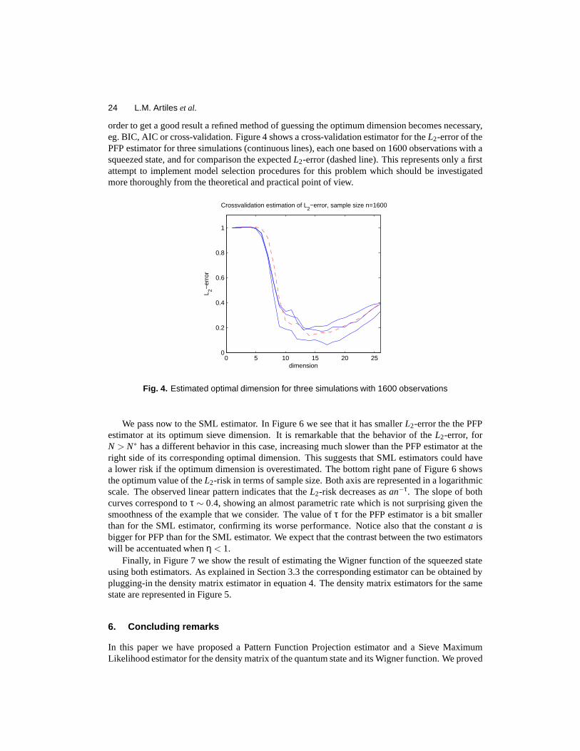
order to get a good result a refined method of guessing the optimum dimension becomes necessary,eg. BIC, AIC or cross-validation. Figure 4 shows a cross-validation estimator for theL2-error of thePFP estimator for three simulations (continuous lines), each one based on 1600 observations with asqueezed state, and for comparison the expectedL2-error (dashed line). This represents only a firstattempt to implement model selection procedures for this problem which should be investigatedmore thoroughly from the theoretical and practical point ofview.

0 5 10 15 20 250

0.2

0.4

0.6

0.8

1

dimension

L 2−er

ror

Crossvalidation estimation of L2−error, sample size n=1600

Fig. 4. Estimated optimal dimension for three simulations with 1600 observations

We pass now to the SML estimator. In Figure 6 we see that it has smallerL2-error the the PFPestimator at its optimum sieve dimension. It is remarkable that the behavior of theL2-error, forN > N∗ has a different behavior in this case, increasing much slower than the PFP estimator at theright side of its corresponding optimal dimension. This suggests that SML estimators could havea lower risk if the optimum dimension is overestimated. The bottom right pane of Figure 6 showsthe optimum value of theL2-risk in terms of sample size. Both axis are represented in a logarithmicscale. The observed linear pattern indicates that theL2-risk decreases asan−τ. The slope of bothcurves correspond toτ ∼ 0.4, showing an almost parametric rate which is not surprisinggiven thesmoothness of the example that we consider. The value ofτ for the PFP estimator is a bit smallerthan for the SML estimator, confirming its worse performance. Notice also that the constanta isbigger for PFP than for the SML estimator. We expect that the contrast between the two estimatorswill be accentuated whenη < 1.

Finally, in Figure 7 we show the result of estimating the Wigner function of the squeezed stateusing both estimators. As explained in Section 3.3 the corresponding estimator can be obtained byplugging-in the density matrix estimator in equation 4. Thedensity matrix estimators for the samestate are represented in Figure 5.

6. Concluding remarks

In this paper we have proposed a Pattern Function Projectionestimator and a Sieve MaximumLikelihood estimator for the density matrix of the quantum state and its Wigner function. We proved


Fig. 5. Estimation of Squeezed state. First column, from top to bottom, PFP and SML estimators.Second column, corresponding errors

they are consistent for different norms in their corresponding spaces. There are many open statisticalquestions related to quantum tomography and we would like toenumerate a few of them here.

• Cross-validation.For both types of estimators, a data dependent method is needed for select-ing the optimal sieve dimension. We mention criteria such asunbiased cross-validation, hardthresholding or other types of minimum contrast estimatorsBarron et al. (1999).

• Efficiency0< η < 1. A realistic detector has detection efficiency 0< η < 1 which introducesan additional noise in the homodyne data. From the statistical point of view we deal with aGaussian deconvolution problem on top of the usual quantum tomography estimation.

• Rates of convergence.Going beyond consistency requires the selection of classesof stateswhich are natural both from the physical, as well as statistical point of view. One shouldstudy optimal and achieved rates of convergence for given classes. For 0< η < 1 the ratesare expected to be significantly lower than in the ideal case,so it becomes even more crucialto use optimal estimators. In applications, sometimes onlythe estimation of a functional ofρ such as average number of photons or entropy may be needed. This will require a separateanalysis, cf. Shen (2001).


Fig. 6. L2 error for Pattern Function Estimator and Sieve Maximum Likelihood Estimator and differentsample sizes: n = 100, . . . ,12800. Last graphic represents the optimum L2 error for different samplesize, using a logarithmic scale on both axis.

• Kernel estimators for Wigner function.When estimating the Wigner function it seems morenatural to use a kernel estimator such as in Cavalier (2000) and to combine this analysis withthe deconvolution problem in the case noisy observationsη < 1, Butucea (2004).

• Other quantum estimation problems.The methods used here for quantum tomography canbe applied in other problems of quantum estimation, such as for example the calibration ofmeasurement devices or the estimation of transformation ofstates under the action of quantummechanical devices.

References

Banaszek, K., D’Ariano, G. M., Paris, M. G. A., and Sacchi, M.F. (1999). Maximum-likelihoodestimation of the density matrix.Phys. Rev. A 61, R010304.


Fig. 7. Graphical representation of Wigner functions estimation. a) Original Wigner function of thesqueezed state, b) Pattern Function estimation, c) Maximum Likelihood estimation

Barndorff-Nielsen, O. E., Gill, R., and Jupp, P. E. (2003). On quantum statistical inference (withdiscussion).J. Royal Stat. Soc. B 65, 775–816.

Barron, A. R., Birge, L., and Massart, P. (1999). Risk bounds for model selection via penalization.Probab. Theory Relat. Fields 113, 301–413.

Butucea, C. (2004). Deconvolution of supersmooth densities with smooth noise.The CanadianJournal of Statistics 32. to appear.

Cavalier, L. (2000). Efficient estimation of a density in a problem of tomography.Ann. Statist. 28,630–647.

D’Ariano, G. M. (1995). Tomographic measurement of the density matrix of the radiation field.Quantum Semiclass. Optics 7, 693–704.

D’Ariano, G. M., Leonhardt, U., and Paul, H. (1995). Homodyne detection of the density matrix ofthe radiation field.Phys. Rev. A 52, R1801–R1804.

D’Ariano, G. M., Macchiavello, C., and Paris, M. G. A. (1994). Detection of the density matrixthrough optical homodyne tomography without filtered back projection. Phys. Rev. A 50, 4298–4302.

Deans, S. R. (1983).The Radon transform and some of its applications. John Wiley & Sons, NewYork.

Dempster, A. P., Laird, N. M., and Rubin, D. B. (1977). Maximum likelihood from incomplete datavia the EM algorithm (with discussion).J. R. Statist. Soc. B 39, 1–38.

Guta, M. I. (2004). Quantum tomography. in preparation.

Helstrom, C. W. (1976).Quantum Detection and Estimation Theory. Academic Press, New York.

Holevo, A. S. (1982).Probabilistic and Statistical Aspects of Quantum Theory. North-Holland.

Leonhardt, U. (1997).Measuring the Quantum State of Light. Cambridge University Press.


Leonhardt, U., Munroe, M., Kiss, T., Richter, Th., and Raymer, M. G. (1996). Sampling of photonstatistics and density matrix using homodyne detection.Optics Communications 127, 144–160.

Leonhardt, U., Paul, H., and D’Ariano, G. M. (1995). Tomographic reconstruction of the densitymatrix via pattern functions.Phys. Rev. A 52, 4899–4907.

Shen, X. (2001). On Bahadur efficiency and maximum likelihood estimation in general parameterspaces.Statistica Sinica 11, 479–498.

Simon, B. (1979).Trace Ideals and their Applications. Cambridge University Press.

Smithey, D. T., Beck, M., Raymer, M. G., and Faridani, A. (1993). Measurement of the Wigner dis-tribution and the density matrix of a light mode using optical homodyne tomography: Applicationto squeezed states and the vacuum.Phys. Rev. Lett. 70, 1244–1247.

van de Geer, S. (2000).Applications of Empirical Process Theory. Cambridge University Press.

Vardi, Y., Shepp, L. A., and Kaufman, L. (1985). A statistical model for positron emission tomog-raphy.J. Am. Stat. Assoc. 80, 8–37.

Williams, D. (1991).Probability with Martingales. Cambridge University Press.

Wong, W. H. and X. Shen (1995). Probability inequalities forlikelihood rations and convergencerates of sieve MLEs.Ann. Statist. 23(2), 339–362.

An invitation to quantum tomography

Documents

Transcript of An invitation to quantum tomography