Real-time Ray Tracing on the GPU

Ray Tracing using CUDA and kD-Trees

DIPLOMARBEIT

zur Erlangung des akademischen Grades

Diplom-Ingenieur

im Rahmen des Studiums

Visual Computing

eingereicht von

Günther VoglsamMatrikelnummer 9955844

an derFakultät für Informatik der Technischen Universität Wien

Betreuung: Associate Prof. Dipl.-Ing. Dipl.-Ing. Dr.techn. Michael WimmerMitwirkung: Dipl.-Ing. Dr. Robert F. Tobler

Wien, 29.04.2013(Unterschrift Günther Voglsam) (Unterschrift Betreuung)

Technische Universität WienA-1040 Wien Karlsplatz 13 Tel. +43-1-58801-0 www.tuwien.ac.at

Real-time Ray Tracing on the GPU

Ray Tracing using CUDA and kD-Trees

MASTER’S THESIS

submitted in partial fulfillment of the requirements for the degree of

Diplom-Ingenieur

in

Visual Computing

by

Günther VoglsamRegistration Number 9955844

to the Faculty of Informaticsat the Vienna University of Technology

Advisor: Associate Prof. Dipl.-Ing. Dipl.-Ing. Dr.techn. Michael WimmerAssistance: Dipl.-Ing. Dr. Robert F. Tobler

Vienna, 29.04.2013(Signature of Author) (Signature of Advisor)

Technische Universität WienA-1040 Wien Karlsplatz 13 Tel. +43-1-58801-0 www.tuwien.ac.at

Erklärung zur Verfassung der Arbeit

Günther VoglsamHubertusstrasse 7, 4470 Enns

Hiermit erkläre ich, dass ich diese Arbeit selbständig verfasst habe, dass ich die verwende-ten Quellen und Hilfsmittel vollständig angegeben habe und dass ich die Stellen der Arbeit -einschließlich Tabellen, Karten und Abbildungen -, die anderen Werken oder dem Internet imWortlaut oder dem Sinn nach entnommen sind, auf jeden Fall unter Angabe der Quelle als Ent-lehnung kenntlich gemacht habe.

(Ort, Datum) (Unterschrift Günther Voglsam)

i

Acknowledgements

I want to thank Michael Wimmer at the Institute of Computergraphics and Algorithms for hissupport for the thesis, as well as the members of the VRVis Forschungs-GmbH for making thisthesis happen in such a pleasant environment. At the VRVis I want to say special thanks toRobert F. Tobler, Michael Schwärzler and Christian Luksch for all their support and the numer-ous discussions we had.

I also want to thank the Faculty of Computer Science at the Vienna University of Technologyfor the financial support to acquire the needed hardware to make this thesis happen.

Finally I’d like to thank my colleagues from the Computer Graphics Club for all the inter-esting discussions and their friendship.

iii

Abstract

In computer graphics, ray tracing is a well-known image generation algorithm which existssince the late 1970s. Ray tracing is typically known as an offline algorithm, which means thatthe image generation process takes several seconds to minutes or even hours or days.

In this thesis I present a ray tracer which runs in real-time. Real-time in terms of computergraphics means that 60 or more images per second (frames per second, FPS) are created. Toachieve such frame rates, the ray tracer runs completely on the graphics card (GPU). This ispossible by making use of Nvidia’s CUDA -API. With CUDA, it is possible to program theprocessor of a graphics card similar to a processor of a CPU. This way, the computational powerof a graphics card can be fully utilized. A crucial part of any ray tracer is the acceleration datastructure (ADS) used. The ADS is needed to efficiently search in geometric space. In this thesis,two variants of so called kD-Trees have been implemented. A kD-Tree is a binary tree, whichdivides at each node a given geometric space into two halves using an axis aligned splittingplane.

Furthermore, a CUDA library for the rendering engine Aardvark, which is the in-houserendering engine at the VRVis Research Center, was developed to access CUDA functionalityfrom within Aardvark in an easy and convenient way.

The ray tracer is part of a current software project called “HILITE” at the VRVis ResearchCenter.

v

Kurzfassung

Die Strahlen-Verfolgung („Ray-Tracing“) ist ein Verfahren zur Berechnung von Bildern, dassseit den späten 1970er-Jahren bekannt ist. Dieses Verfahren ist typischerweise ein so genann-ter „off-line“ Algorithmus, was bedeutet, dass die Berechnung für ein Bild zwischen mehrerenSekunden oder Minuten bis hin zu mehreren Stunden oder gar Tagen benötigen kann.

Im Zuge dieser Diplomarbeit wurde ein Programm zur Strahlen-Verfolgung („Raytracer“)entwickelt, der die Erzeugung von Bildern in Echtzeit ermöglicht. „Echtzeit“ im Sinne derComputer-Graphik bedeutet dabei, 60 oder mehr Bilder pro Sekunde berechnen und anzeigen zukönnen. Um solch hohe Bilderzeugungsraten erreichen zu können, wird der Raytracer komplettauf der Graphikkarte (GPU) ausgeführt. Ermöglicht wird dies durch verwenden der Technolo-gie CUDA. CUDA wurde vom Graphikkarten-Hersteller Nvidia entwickelt und erlaubt es, denProzessor einer Graphikkarte in ähnlicher Art und Weise zu programmieren wie den einer CPU.Damit ist es möglich, die volle Rechenleistung einer Graphikkarte auszunutzen. Ein wichtigerTeil eines Raytracers sind dessen Beschleunigungsdatenstrukturen. Diese werden verwendet,um das Aufsuchen von Objekten im geometrischen Raum zu beschleunigen. In dieser Diplom-arbeit wurden so genannte kD-Bäume in zwei unterschiedlichen Varianten implementiert. EinkD-Baum ist ein binärer Baum, bei dem jeder Knoten einen gegebenen geometrischen Raumdurch achsparallele Ebenen in zwei Unterräume teilt.

Zusätzlich wurde für die Programmierung des Raytracers eine CUDA Bibliothek für „Aard-vark“ entwickelt. Aardvark ist die hauseigene Rendering-Engine des VRVis Forschungs-GmbH.Die Bibliothek erlaubt es, CUDA-Funktionalität innerhalb von Aardvark ohne großen Initialauf-wand verwenden zu können.

Der Raytracer ist Teil eines größeren Software-Projekts namens „HILITE“, welches am VR-Vis umgesetzt wird.

vii

For my grandfather

Albert Weichhart

1919 - 2012

Contents

1 Introduction 11.1 About Ray Tracing . . . . . . . . . . . . . . . . . . . . . . . . . . . . . . . . 11.2 Programmable Graphics Hardware and Ray Tracing . . . . . . . . . . . . . . . 31.3 Aim of the Thesis . . . . . . . . . . . . . . . . . . . . . . . . . . . . . . . . . 41.4 Contributions . . . . . . . . . . . . . . . . . . . . . . . . . . . . . . . . . . . 4

1.4.1 CUDA Library . . . . . . . . . . . . . . . . . . . . . . . . . . . . . . 51.4.2 CUDA Ray tracer . . . . . . . . . . . . . . . . . . . . . . . . . . . . . 51.4.3 Über-kD-Tree . . . . . . . . . . . . . . . . . . . . . . . . . . . . . . . 61.4.4 A new debugging Method . . . . . . . . . . . . . . . . . . . . . . . . 61.4.5 Presentation of Algorithms for the GPU . . . . . . . . . . . . . . . . . 7

2 Theory 92.1 The Rendering Equation . . . . . . . . . . . . . . . . . . . . . . . . . . . . . 9

2.1.1 BRDF, BTDF, BSDF . . . . . . . . . . . . . . . . . . . . . . . . . . . 112.1.2 Solution Attempts of the Rendering Equation . . . . . . . . . . . . . . 12

2.2 Light Transport Notation . . . . . . . . . . . . . . . . . . . . . . . . . . . . . 142.3 The Ray Tracing Algorithm . . . . . . . . . . . . . . . . . . . . . . . . . . . . 14

2.3.1 Overview . . . . . . . . . . . . . . . . . . . . . . . . . . . . . . . . . 142.3.2 Basic Ray Tracing Algorithm . . . . . . . . . . . . . . . . . . . . . . 16

3 Background and Related Work 233.1 Acceleration Data Structures for Ray Tracing . . . . . . . . . . . . . . . . . . 23

3.1.1 Motivation . . . . . . . . . . . . . . . . . . . . . . . . . . . . . . . . 233.1.2 Brute Force . . . . . . . . . . . . . . . . . . . . . . . . . . . . . . . . 233.1.3 KD-Trees . . . . . . . . . . . . . . . . . . . . . . . . . . . . . . . . . 243.1.4 Bounding Volume Hierarchies . . . . . . . . . . . . . . . . . . . . . . 313.1.5 Other Common Acceleration Data Structures . . . . . . . . . . . . . . 323.1.6 Divide-and-Conquer Schemes . . . . . . . . . . . . . . . . . . . . . . 323.1.7 Splitting Strategies . . . . . . . . . . . . . . . . . . . . . . . . . . . . 34

3.2 CUDA . . . . . . . . . . . . . . . . . . . . . . . . . . . . . . . . . . . . . . . 393.2.1 Motivation for General Purpose Programming on Graphics Hardware . 393.2.2 CUDA . . . . . . . . . . . . . . . . . . . . . . . . . . . . . . . . . . 393.2.3 CUDA and OpenCL . . . . . . . . . . . . . . . . . . . . . . . . . . . 46

xi

4 Ray Tracing on the GPU 494.1 Advent of Real-Time Ray Tracing . . . . . . . . . . . . . . . . . . . . . . . . 494.2 Iterative Ray Tracing . . . . . . . . . . . . . . . . . . . . . . . . . . . . . . . 514.3 Parallel Ray Tracing . . . . . . . . . . . . . . . . . . . . . . . . . . . . . . . 514.4 KD-Trees for GPUs . . . . . . . . . . . . . . . . . . . . . . . . . . . . . . . . 53

4.4.1 Stack-based Iterative Traversal . . . . . . . . . . . . . . . . . . . . . . 534.4.2 KD-Restart . . . . . . . . . . . . . . . . . . . . . . . . . . . . . . . . 534.4.3 KD-Backtrack . . . . . . . . . . . . . . . . . . . . . . . . . . . . . . 554.4.4 Short-Stack and Push-Down . . . . . . . . . . . . . . . . . . . . . . . 55

4.5 Über-kD-Tree . . . . . . . . . . . . . . . . . . . . . . . . . . . . . . . . . . . 56

5 CUDA Library 575.1 Overview . . . . . . . . . . . . . . . . . . . . . . . . . . . . . . . . . . . . . 575.2 Host Side . . . . . . . . . . . . . . . . . . . . . . . . . . . . . . . . . . . . . 58

5.2.1 Management . . . . . . . . . . . . . . . . . . . . . . . . . . . . . . . 585.2.2 Built-In Data-Types . . . . . . . . . . . . . . . . . . . . . . . . . . . 635.2.3 Graphics-Resource Sharing . . . . . . . . . . . . . . . . . . . . . . . 64

5.3 Device Side . . . . . . . . . . . . . . . . . . . . . . . . . . . . . . . . . . . . 655.4 Examples . . . . . . . . . . . . . . . . . . . . . . . . . . . . . . . . . . . . . 65

6 CUDA Ray Tracer 676.1 Overview . . . . . . . . . . . . . . . . . . . . . . . . . . . . . . . . . . . . . 676.2 Program Flow . . . . . . . . . . . . . . . . . . . . . . . . . . . . . . . . . . . 686.3 The CUDA Ray Tracing Kernel . . . . . . . . . . . . . . . . . . . . . . . . . 686.4 Acceleration Data Structures . . . . . . . . . . . . . . . . . . . . . . . . . . . 69

6.4.1 Creation and Conversion . . . . . . . . . . . . . . . . . . . . . . . . . 706.4.2 Scene Traversal . . . . . . . . . . . . . . . . . . . . . . . . . . . . . . 72

6.5 Runtime Parameters . . . . . . . . . . . . . . . . . . . . . . . . . . . . . . . . 746.6 Debugging . . . . . . . . . . . . . . . . . . . . . . . . . . . . . . . . . . . . . 74

7 Results 777.1 Test Setup . . . . . . . . . . . . . . . . . . . . . . . . . . . . . . . . . . . . . 777.2 Results . . . . . . . . . . . . . . . . . . . . . . . . . . . . . . . . . . . . . . . 777.3 KD-Tree vs. Über-kD-Tree . . . . . . . . . . . . . . . . . . . . . . . . . . . . 837.4 Lessons learned . . . . . . . . . . . . . . . . . . . . . . . . . . . . . . . . . . 83

8 Conclusion and Future Work 898.1 Conclusion . . . . . . . . . . . . . . . . . . . . . . . . . . . . . . . . . . . . 898.2 Future Work . . . . . . . . . . . . . . . . . . . . . . . . . . . . . . . . . . . . 90

Bibliography 93

xii

CHAPTER 1Introduction

1.1 About Ray Tracing

Ray tracing is one of the classic rendering algorithms. It arose already in the late 1970s. Raytracing simulates the transport of light in a scene by shooting rays of light from the eye-pointinto the scene. Those rays are then intersected with the scene objects. If a ray hits a surfacewhich is reflective like a mirror, the ray bounces off the surface and the path of the ray is furthertraced. Moreover, if a ray hits an object made of a transparent material, the ray gets refractedand is traced through this transparent object. However, when the ray hits an object with diffusematerial or no object at all, the tracing of the ray stops. Figure 1.2 shows the basic ray-tracingscheme and Figure 1.1 shows a typical example of a ray-traced image. The strength of raytracing is that it can generate images with correct reflection and correct refraction, as well ascorrect hard shadows, with relatively low programming effort in contrast to rasterization (seebelow). The basic ray-tracing algorithm is described in detail in Section 2.3 and throughout thethesis, various properties are discussed with particular attention paid to real-time ray tracing.

1

Figure 1.1: Example ray tracing image. [Tra06]

Eye Light SourceImage Plane

diuse Material

specular Material

transparent Material

Scene Objects

Figure 1.2: Ray-tracing scheme. Light rays are traced from the eye-point into the scene througheach pixel. The rays are intersected with the objects in the scene and if the object’s material iseither reflecting or transparent, one or more follow-up rays are traced.

2

As opposed to ray tracing, rasterization has been the dominant rendering algorithm for sev-eral decades. In order to generate an image using rasterization, the whole scene geometry isprojected onto the image plane. For each pixel, it is determined which polygon covers the spaceof the pixel. To ensure that polygons farther away do not overwrite pixels of polygons nearer tothe image plane, a depth buffer is maintained. The depth buffer stores for each pixel the distanceof the polygon currently drawn at this pixel. Using a depth test, the polygons which are fartheraway than the one at the corresponding location in the depth buffer are discarded, and thereforeonly the polygons nearest to the image plane are drawn.

Graphics cards are highly optimized for rendering using rasterization. However, dealing withrasterization becomes tricky when images with a realistic look are desired. Therefore, severalextension algorithms have been invented to render effects like shadows, reflection, refraction,depth-of-field and others. These algorithms are usually either hard to implement, computation-ally expensive or do not meet the desired image quality because of algorithmic simplifications.Many of those effects like correct reflection and refraction as well as hard shadows, however,come naturally with the ray-tracing algorithm, and other effects can be implemented into a raytracer without much effort.

1.2 Programmable Graphics Hardware and Ray Tracing

Looking at the evolution of graphics cards during the last decade, they became more and moreflexible and programmable. Instead of using only a hard-wired pipeline for rendering images, theso-called fixed function pipeline, nowadays this pipeline can be programmed at several stages.This flexibility eventually led to the point where graphics cards were fully programmable. Fiveyears ago, the graphics cards vendor Nvidia supplied an API called CUDA for accessing theirfully programmable hardware to make use of the computational power of these graphics cardsfor other purposes than rendering using rasterization.

The original purpose of graphics cards was calculating a color for each pixel on the screen.This can be done in a parallel manner, and, due to this fact, graphics cards are highly parallel pro-cessors. Also, ray tracing can be calculated in parallel by many independent threads or proces-sors. Hence, calculating ray-traced images on those fully programmable graphics cards insteadon CPUs became an interesting topic. However, the hardware architecture of graphics cards wasnot perfectly suited for ray tracing, mainly because random memory accesses were comparablyslow in graphics memory as opposed to CPU-RAM. Latest graphics cards generations try toremedy this drawback by implementing faster memory access and a cache hierarchy [Coo10].

Depending on the complexity of the scene, a ray-traced image can take from a few seconds orminutes, up to several hours or even more to render. In computer graphics, the term “real-time”usually refers to a frequency of 60 or more images per second, each of which has to be generatedby the application. The frequency at which the images can be generated is called the frame rate.It is often expressed in frames per second (FPS). Even on a modern high-end computer, it isvery hard to achieve such high frame rates using the CPU to ray trace an image. But whenexploiting the computational power of modern, massively parallel GPUs, these frame rates canbecome possible. However, this still depends highly on the complexity of the scene and the

3

concrete implementation, as well as on the used acceleration structures and other optimizations(see Chapter 3.1), but real-time ray tracing is possible nowadays.

1.3 Aim of the Thesis

This thesis is part of the HILITE project [Gmb] at the VRVis Forschungs-GmbH. The aimof this project is to give a highly realistic, interactively modifiable preview of the illumina-tion of architectural scenes. The main lighting computations are done using advanced raster-ization techniques like GPU-based light simulation using lightmaps, together with a photonsimulation done on the CPU. Since reflections are view-dependent and the application is in-teractive, correct reflections cannot be precalculated when moving through the scene. Sev-eral attempts have been made to render correct reflections on curved surfaces with rasteriza-tion [EMD+05] [EMDT06] [RH06]. All these methods, however, are either not accurate enough,can not handle concave geometry or can not handle 2nd-order reflections. Therefore, a real-timeray tracer was needed. The idea was to integrate the ray tracer into the rasterization-basedalgorithms to form a hybrid rendering system. Attempts for hybrid rendering systems as a com-bination of rasterization and ray tracing have been done already by Beister et al. [MB05] andCabeleira [Cab10]. Both utilized the rasterization algorithm on the GPU to generate an imageand enhanced it with a ray tracer running on the CPU, which is in both cases only capable ofcreating first-hit reflections and refractions.

The goal of this thesis was to realize a ray tracer on the GPU which is capable of runningat interactive to real-time frame rates. The implementation of the whole ray tracer on the GPUled to several challenging tasks. The first one is that the GPU can run many (up to thousands) ofthreads in parallel, which made new designs of the implemented algorithms necessary. Further-more, recursion was not or not sufficiently supported at the time of implementing the ray tracer.This required iterative solutions. Finally, the development tools for GPU programming are notthat advanced yet as they are for the CPU. Hence, the lack of debugging possibilities made ithard to debug a bigger program running entirely on the GPU. Solutions for that are presented inSection 6.6.

As a prerequisite to implementing a GPU ray tracer, a library for accessing the GPU com-puting capabilities from within the VRVis-internal rendering engine Aardvark was needed. Thegoal was further to provide easy, high-level access to CUDA through this library. Based on thisCUDA library, a CUDA ray tracer has been developed. It was designed in such a way that it canbe used from within any Aardvark application. Furthermore, since the ray tracer should be ableto integrate into the main program of the HILITE project, the HILITE-Viewer, an interface anddata conversion should be provided by the ray tracer, which proved to be a demanding task. TheCUDA library will be described in detail in Chapter 5 and the CUDA ray tracer in Chapter 6.

1.4 Contributions

This thesis has two contributions of a more practical nature and three contributions which canbe called scientific. They will be summarized in this section.

4

1.4.1 CUDA Library

The first contribution is a CUDA library developed for the VRVis-internal rendering engineAardvark. Aardvark is used as a base framework for many scientific projects. The CUDAlibrary now makes it possible to utilize the power of GPU computing for various projects. Oneof those projects is the CUDA ray tracer, which was also developed for this thesis (see nextcontribution).

The CUDA library provides access to CUDA-functionality on a high level of abstractionfrom within Aardvark, which is written in C#. The library is explained in detail in Chapter 5.The most important features of the library are:

• Management of CUDA-Context, -Device, -Modules and -Functions: By using the library,CUDA contexts can be created easily as well as modules and functions can be loaded in aconvenient way.

• Memory manager: The CUDA resources are managed with a memory manager, whichautomatically cleans up unused resources on the GPU.

• Data types: Ready-to-use data types for arrays and struct-like data are provided. Thosedata types can be worked with as with normal C#-data types and are automatically madeavailable for inside a CUDA kernel. Page-locked arrays are supported too.

• Simple kernel launch: The launch of a CUDA kernel can be done almost as simple ascalling any C#-function.

• Graphics resource sharing: DirectX graphics resources, like textures and buffers, can beshared with CUDA. Functionality for sharing of OpenGL resources can be added withvery little effort as well.

• Full support for CUDA-Streams, CUDA-Events and -Timers, and so on. Almost everyfeature of the CUDA API 3.x is available via the CUDA library.

1.4.2 CUDA Ray tracer

The second contribution is the CUDA ray tracer itself. It is called CURA and utilizes the CUDAlibrary. CURA will be described in detail in Chapter 6. Some of the features are:

• A ray tracer which runs completely on the GPU, so the CPU is free for other tasks.

• Real-time to interactive frame rates, depending on the scene complexity.

• The ray tracer uses kD-Trees in two variants:

– Object-kD-Tree: One kD-Tree per scene object.

– Über-kD-Tree: One kD-Tree for the whole scene. The leaves of this tree are theObject-kD-Trees.

Both are described in Sections 6.4 and 7.3.

5

• The main purpose of the ray tracer is to render static scenes, however, scene updates andhence animations are supported as well.

• The used graphics resources are shared between CUDA and Direct X for efficient render-ing.

• Fully configurable at runtime.

• Since the implemented ray tracer can be used by any Aardvark application, CURA servesas an example on how to use the CUDA ray tracer inside Aardvark projects.

• Last but not least, the ray tracer has already been built into the HILITE-Viewer by anotherstudent concurrently to writing this thesis.

1.4.3 Über-kD-Tree

One of our contributions is a new data structure which we call the Über-kD-Tree. It is a kD-Treewith kD-Trees in its leaves. The leaf kD-Trees are kd-Trees per geometrical object and we callthem Object-kD-Tree. The main reason why we developed this data structure is that in the finalapplication, the HILITE-Viewer, objects need to be added and deleted interactively at runtime.To spare costly rebuilds of data structures in case of an addition or deletion of an object, just theusually small Über-kD-Tree needs to be rebuilt, which can be done quite fast.

The Über-kD-Tree is described in Section 4.5, details on the implementation are given inSection 6.4 and results using this data structure are presented in Section 7.3.

1.4.4 A new debugging Method

Debugging kD-Trees is hard, and it is even harder when they are implemented on the GPU, forseveral reasons. First, on the GPU a kD-Tree or any other data structure is “flattened” to an arrayand uses indices as pointers between the nodes. This makes traversing the data structure harderbecause indices, which also encode leaves, have to be processed. Second, recursive functioncalls are nowadays supported on GPUs, but slow. Hence, iterative methods have to be usedwhich leads in turn to several special cases which occur only seldom.

Since GPU debugging capabilities are still limited, the only way to debug such code is torewrite the GPU code for the CPU and debug it there. However, an image to be rendered consistsof a few-thousand to a few-million pixels and only some of them exhibit erroneous results. Forthis reason it is not possible nor necessary to debug the complete rendering of the whole image.

As a solution to this, I introduced the so-called “debug pixel”. It is one pixel fixed on thescreen for which debugging can be triggered on the CPU. When moving around with the camerain the scene, one can point the debug pixel to a pixel which shows a wrong result and triggerdebugging for this pixel only. This way, special cases can be debugged well.

The debug method is further described in Section 6.6.

6

1.4.5 Presentation of Algorithms for the GPU

There are several papers released which deal with real-time ray tracing on the GPU. However,it is hard to find information on complete algorithms for GPUs, especially iterative and parallelversions of the ray tracing algorithm for CUDA, as well as several techniques for the traversalof kD-Trees. For this reason, Chapter 4 describes and summarizes the complete algorithms foriterative and parallel ray tracing for GPUs and several traversal methods for GPUs for kD-Trees.

7

CHAPTER 2Theory

In this chapter, the theoretical foundations for generating an image from virtual scenes are ex-plained. First, the rendering equation is introduced. Ray tracing provides a partial solution tothe rendering equation. Later on, an overview is given on how to model properties of materialsbefore presenting methods of practical solutions of the rendering equation. For the classificationof rendering algorithms, the light transport notation is presented. Finally, the basic ray-tracingalgorithm is explained in detail in the last section of this chapter.

2.1 The Rendering Equation

In order to generate realistic-looking images, the propagation of light in a scene has to be cal-culated. The rendering equation is a mathematical formulation of how light disperses in a sceneand can be used to classify diverse rendering algorithms, depending on which parts of the render-ing equation the algorithms can solve, approximate or which parts are omitted. The renderingequation was published simultaneously by Kajiya [Kaj86] and Immel et al. [ICG86] in 1986.Equation 2.1 shows the original Kajiya version.

I(x, x′) = g(x, x′) [ε(x, x′) +

∫S

ρ(x, x′, x′′)I(x′, x′′) dx′′]. (2.1)

whereI(x, x′) is the intensity of light passed from point x′ to point x,

g(x, x′) is a geometry term which encodes the occlusion between the two points,

ε(x, x′) is the emitted light from point x′ to x,

S is the union of all surfaces in the scene and

ρ(x, x′, x′′) is the intensity of the light scattered from x′′ to x via x′. ρ is the BRDF.

9

The alternative and nowadays more common form of the rendering equation from Immel etal. [ICG86] is as follows:

Lo(p, ωo) = Le(p, ωo) + Ls(p, ωo). (2.2)

whereLo(p, ωo) is the outgoing radiance from point p in the direction of ωo,

Le(p, ωo) is the emitted radiance from point p in the direction of ωo and

Ls(p, ωo) is the scattered radiance from p in the direction of ωo.

Ls itself can be expanded to

Ls(p, ωo) =

∫Ω

ρ(p, ωi, ωo)Li(p, ωi) cosθ dωi. (2.3)

where

Ω is the hemisphere of the incoming radiance,

ρ(p, ωi, ωo) is the amount of the reflected radiance at point p for incoming radiance withangle ωi and outgoing radiance with angle ωo. This is the BRDF.

Li(p, ωi) is the incoming radiance at point p from direction ωi. It can also be seen as theoutgoing radiance from a point p′ with angle −ωi, thus Li(p, ωi) = Lo(p

′,−ωi). This is in turnthe same as the first hit of a ray from the point p in the direction ωi. It is usually expressed bythe visibility function h with p′ = h(p,−ωi), which then gives Lo(p

′,−ωi) = Lo(h(p,−ωi), ωi)(see Figure 2.1, left) [Lás99].

cos θ corresponds to the geometric term from Kajiya’s rendering equation. θ is the angle ofincident, which is the angle between the surface normal at point p and the incoming radiance.Thus, if the angle increases, the available energy is distributed over a greater area, decreasingthe amount of energy per unit area (see Figure 2.1, right).

It is hard to solve the rendering equation analytically. One problem is the recursion. Everyincoming radiance Li at point p is the Lo of another point p′, which in term has other incomingLi’s of other points p′′, and so on. Because of the law of conservation of energy, no additionalenergy can be produced or emitted at a recursion level, but energy can be absorbed by thematerial. This means that the deeper the level of recursion, the lower the available energy, andthus the contribution to the final image is also comparatively small. Some rendering algorithmstherefore stop the recursion either at a fixed maximum level, or if the energy of a recursion levelis below a certain threshold.

Another problem is that the integral over the hemisphere Ω has infinitely many incomingdirections. This is the reason why the hemisphere can only be approximated by sampling.

10

L o(p, ωo)

L i (p, ω i) = L o( , ω )Ω

θ

p

p’

i ih(p, − ω )

θFigure 2.1: Left: Incoming and outgoing radiance at point p from point p′. Right: Cos θ-Term.If the incident angle θ increases, the amount of energy per unit area decreases. (Figures adaptedfrom [Gue08].)

2.1.1 BRDF, BTDF, BSDF

BRDF is the abbreviation for bidirectional reflectance distribution function. It is used to describethe reflection characteristics of a surface, i.e., it describes how incident light is scattered andreflected. Since light can only be reflected into the upper hemisphere, the BRDF is defined onlyfor this region. Formally, the BRDF is a function which takes four parameters, the incoming andoutgoing directions in spherical coordinates (Equation 2.4). If the two-dimensional position ona surface is included, the BRDF has six parameters, as in the rendering equation (Equation 2.1).

ρ(ωi, ωo) =Lo(ωo)

Li(ωi) cosθi dωi. (2.4)

BRDFs must fulfill several properties to be called physically plausible [Lás99]. First, aBRDF must satisfy the Helmholtz reciprocity, which means that the BRDF is symmetric withregard to the incoming and outgoing directions:

ρ(ωi, ωo) = ρ(ωo, ωi). (2.5)

This property is important, because this allows ray tracing to be performed in the opposite(backward) direction. Furthermore, a BRDF must satisfy the law of energy conservation. Thismeans that the reflected amount of light is less or equal to the incoming light:∫

Ω

ρ(ωi, ωo) ≤ 1. (2.6)

A BRDF for a material with perfect specular reflection reflects the light in one directiononly. If a material exhibits perfect diffuse reflection, light is scattered equally in all directionsinto the upper hemisphere. Real-world materials, however, consist of a combination of diffuseand specular reflection properties, like rough specular or directional diffuse materials (see Fig-ure 2.2). To model realistic-looking surfaces, models can be created by measuring the behavior

11

ideal specular

rough specular directional diuse

ideal diuse

Figure 2.2: Reflection and scattering. Ideal specular reflection reflects light only in one direction,whereas an ideal diffuse surface scatters the incoming light equally in all directions. Real-world materials, however, are a combination of both, like a rough specular or directional diffusematerial.

Lambertian Phong Oren-Nayar Cook-Torrance AnisotropicCook-Torrance

Figure 2.3: BRDF examples. Different analytical BRDF-models are shown. [Gue08]

of real materials under defined illumination. The results are then either stored in a table, or ananalytical model is created or fitted to the measured data. Some examples of analytical modelscan be seen in Figure 2.3.

As stated above, BRDFs only describe the reflection into the upper hemisphere. Hence, fortransparent materials, the BTDF, the bidirectional transmittance distribution function, is definedfor the lower hemisphere (the backside, or interior) in a similar way. BRDF and BTDF formfinally together the BSDF, the bidirectional scattering distribution function.

2.1.2 Solution Attempts of the Rendering Equation

Since the rendering equation is hard to solve, several algorithms have been developed whichsimplify the rendering problem and give only an approximate solution. They can be divided into

12

the following three groups [Lás99]:

• Local Illumination methods

The simplest way to solve the rendering equation is by only considering light coming di-rectly from a light source and omitting the light reflected, refracted and scattered betweensurfaces. Because only local properties of the material of the surface and the given lightsource(s) are considered, this type of light is called direct light [Hec90]. Local illumina-tion methods are usually simple and fast to calculate, however, due to simplifications ofthe rendering equation, sacrificing realism of the resulting image.

• Recursive Ray tracing

Recursive ray tracing, also called visibility ray tracing, enhances the local illuminationmodel by allowing recursion of the rendering equation for perfectly reflective and refrac-tive materials. To prevent infinite recursion, usually a maximum recursion depth is de-fined. For recursive ray tracing, the rendering equation can be written as follows [Lás99]:

Lo(p, ωo) = Le(p, ωo) +

∫Ω

ρ(p, ωi, ωo)LLS(h(p,−ωi), ωi) cosθ dωi+

ρr(p, ωr, ωo)Lo(h(p,−ωr), ωr) + ρt(p, ωt, ωo)Lo(h(p,−ωt), ωt).

(2.7)

where

LLS is the incoming radiance from a light source,

ωr and ωt are the ideal directions for reflection and transparency, respectively, and

ρr and ρt are the BRDFs for reflection and transparency.

Hence, recursive ray tracing can handle materials with perfect reflection and refraction.However, diffuse surfaces can still only handle direct light. To be able to also solve thediffuse inter-reflection of surfaces, global illumination solutions are needed. Many ofthose solutions use ray tracing as a basis for the algorithms. The ray tracing algorithmwill be described in detail in the following sections. In this thesis, we will describe theimplementation of a recursive ray tracer. However, it should be possible to use this raytracer also in global illumination solutions.

• Global Illumination solutions

In the real world, light bounces off from surfaces and reflects and refracts not only forperfectly specular or transparent materials, but scatters in various directions, accordingto the type of material. This further means that the illumination of a surface dependsalso on the light bounced off from all other surfaces, the so called indirect light. Hence,for properly solving the rendering equation, this scattering has to be considered as well.

13

Symbols Regular ExpressionsL Light Emission * 0-nD Diffuse reflection or refraction + 1-nS Specular reflection or refraction [] 0-1E Eye interaction | or

() PrecedenceClassification of some rendering algorithmsLDE Ray Casting

LD*E RadiosityL[D]S*E Ray TracingL(D|S)*E Path Tracing; all possible light paths

Table 2.1: Light Transport Notation

Algorithms which are able to calculate indirect lighting are called global illumination al-gorithms. Well known examples are radiosity, path tracing and photon tracing. Figure 2.4shows a comparison of the different solution attempts of the rendering equation. It canbe seen that the more physically correct a rendering solution is, the more time it takes tocompute the image.

2.2 Light Transport Notation

A convenient way to describe the capabilities of different rendering algorithms is to use the lighttransport notation [Hec90]. With a small string, all possible paths of a ray or photon traversingthe scene can be described (see Table 2.1). Letters describe the type of interaction. They canbe combined with symbols to form regular expressions. The capabilities of some well-knownrendering algorithms are also given in Table 2.1.

A path LD*E means that an algorithm is able to handle several bounces of rays or photonsbetween diffuse surfaces, like the classical radiosity algorithm does. All possible paths wouldbe described as L(D|S)*E, which means that there can be arbitrarily many diffuse or specularbounces. Classic ray tracing can handle paths of the form L[D]S*E, which means that whentraced from the eye, there can be many (or none) specular reflections or refractions, but a maxi-mum of only one diffuse bounce. Examples of possible paths are shown in Figure 2.5.

2.3 The Ray Tracing Algorithm

2.3.1 Overview

Ray tracing is a rendering algorithm which simulates the propagation of light in a scene. Raytracing can handle correct reflection and refraction as well as pixel-accurate hard shadows. Byimplementing even more effects, like depth-of-field, motion blur and the like, ray tracing cangenerate realistic-looking images for many types of scenes.

14

local illumination method local illumination method with shadow computation

dohtemnoitanimullilabolggnicart-yarevisrucer

Figure 2.4: Comparison of different rendering solutions. The local illumination took 90 secondsto render (95 seconds with shadows), the ray tracing image was computed in 135 seconds andthe global illumination solution took 9 hours for generating the image. [Lás99]

15

Light Source

Eye

diuse Material

specular Material

LDE

LDSSE

LDSE

LSSE

Figure 2.5: Light Transport Notation showing some possible light paths.

In light transport notation, ray tracing can handle paths of the form L[D]S*E. This meanswhen shooting a ray from the eye, the algorithm can simulate paths of light with multiple (or no)ideal specular reflections until it hits a diffuse surface.

Originally, the light rays have been shot into the scene from the light source. The paths ofthe rays through the scene have been followed until the eye was hit. However, only a few ofthose rays hit the eye and so this approach was wasteful. Therefore, the direction of the rays hasbeen reversed and nowadays the rays are shot from the eye into the scene.

The basic version of the modern ray-tracing algorithm was published in 1979 by TurnerWhitted [Whi80] and is hence often called Whitted style ray tracing. In the following, the basicray-tracing algorithm as well as some extensions will be explained.

2.3.2 Basic Ray Tracing Algorithm

The basic Whitted ray-tracing algorithm is given in Algorithm 1. It starts with creating an eyeray or primary ray for each pixel. The pixels lie in the image plane and therefore the originsof all primary rays lie on this image plane. The exact position of the origins correspond tothe location of the pixels in world space. The direction of the primary rays point from the eyeposition towards the pixel in the image plane (see Figure 2.6).

Then the tracing of the primary ray starts. The ray is intersected with the objects in the sceneand the nearest intersection, if any, is selected. The intersection of the rays with the objects in thescene is the most time-consuming part of the ray tracing algorithm. In the original publication,

16

it consumed 95% of the total run time. Strategy on how to reduce unneccessary intersectionoperations is therefore crucial for reasonable rendering performance for ray tracing. The chapteron acceleration data structures (Chapter 3.1) gives details about various strategies on how toreduce those intersection tests.

If no hitpoint is found, the background color is returned and the calculations for this pixelare finished. If a hit is recorded, shadow tests for all light sources are performed. For this, foreach light source a shadow ray is created. The origin of the shadow ray is the hitpoint of thenearest intersection and the ray’s direction points towards a light source. If there is at least oneobject between the hitpoint and light source, the hitpoint is in shadow with respect to this lightsource. Thus, the hitpoint is not shaded with the given light source. When testing the shadowray for an intersection, the test can be terminated as soon as any intersection is found, which isfaster than looking for the closest intersection. The shadow test is done for all light sources inthe scene. If, however, the hitpoint is visible from a given light source, the hitpoint is shadedwith local shading techniques like Lambert or Phong shading.

The next step is to cast reflected rays, if the material at the hitpoint is specularly reflecting.The origin of the reflected ray is the hitpoint. In ray tracing, all specularly reflecting materialsare ideal. This means that the outgoing direction of the reflection ray encloses the same anglewith the normal of the surface at the hitpoint as the incoming ray (see Figure 2.7, left). Nowthe tracing recursively starts again with the reflected ray as the ray to be processed. When thetracing of this ray, and all rays possibly following due to other reflections or refractions, arecalculated, the tracing stops. There are two common ways to end the recursion of tracing rays.One is to define a maximum recursion level and to stop the recursion when the maximum levelis reached. A maximum level of 2 usually gives already good results. The other way to end therecursion would be a more physically-based one. As mentioned in Section 2.1, the radiance getslower with each bounce. Therefore, one can set a minimum threshold for the contribution andstop the recursion if this threshold is reached.

For transparent materials, refraction rays are traced in a similar way as the reflection rays.The main difference is that the direction for the refraction rays depends on the material proper-ties, more precisely on the index-of-refraction of the material a ray enters and of the material theray is leaving (see Figure 2.7, right).

After all reflection and refraction rays are traced, the final color for this pixel has beencalculated. What remains is to write the color into the output buffer. When a color for all pixelsis calculated, the algorithm has finished and the image can be displayed.

Ray Tree

When a ray hits a transparent object, this ray creates a reflection and a refraction ray. Hence,at every intersection point, a maximum of two follow-up rays can be created. This can berepresented by a binary tree called a ray tree (see Figure 2.8). The root is the primary ray, and ifthis ray hits an object which has a reflecting surface, a reflection ray is created. If the surface isalso transparent, a refraction ray is created as well. In the ray tree, the left child is the reflectionray and the right child the refraction ray [Suf07]. By looking at the ray tree it can be seen thatwith the support for reflection and transparency, a single primary ray can create a deep tree of

17

Light Source

Image Plane

Eye

diuse Material

specular Material

Primary Ray Shadow Ray

Occluded Shadow RaySecundary Ray

Figure 2.6: Basic ray tracing algorithm. Primary rays are sent from the eye through a pixel andintersect the objects in the scene. If a specular material is hit, a reflected ray is created. Finally,when a diffuse material is hit, the shadow rays are cast to test if the given hitpoint is in shadow.

Incoming RayReected Ray

n

θ i θ r θ

n

i

θ t

Incoming RayRefracted Ray

Figure 2.7: Left: Reflection. The outgoing angle is equal to the incident angle for perfectlyspecular materials. Right: Refraction. The angle of the refracted ray depends on the materialproperties of the inner and outer materials.

18

Algorithm 1 Basic Ray Tracing Algorithm (continued on next page)

1: procedure DORAYTRACING()2: for each pixel (x, y)3: primaryRay ← CREATEPRIMRAY(x, y)4: outputColor ← TRACE(primaryRay)5: WRITEOUTPUT(x, y, outputColor)6: end for each7: end procedure8:

9: function CREATEPRIMRAY(x, y)10: origin← point on image plane at pixel (x, y)11: direction← (pixel location in the world) - (eye-point position)12: return Ray(origin, direction)13: end function14:

15: function TRACE(ray)16: color ← black17: hit← INTERSECT(ray, scene)18:

19: if hit then20: color += SHADE(ray, hitPoint)21: if Material is reflective then22: reflectionRay ← Ray(hitPoint, reflected(ray.direction))23: color += TRACE(reflectionRay)24: end if25: if Material is transparent then26: refractionRay ← Ray(hitPoint, refracted(ray.direction))27: color += TRACE(refractionRay)28: end if29: else30: color ← BackgroundColor31: end if32:

33: return color34: end function

rays. Usually a maximum tree level is defined to stop the fan out of the tree and hence omitfurther tracing.

Packet Traversal

The simplest way to trace rays is to trace one by one. However, nearby rays are likely to hitsimilar objects. Hence, it would be beneficial to trace those rays together to utilize cached

19

Algorithm 1 Basic Ray Tracing Algorithm (continued from previous page)

35: function SHADE(ray, hitPoint)36: color ← black37:

38: for each light source39: shadowRay ← Ray(hitPoint, (light source position− hitPoint))40: inShadow ← CASTSHADOWRAY(shadowRay)41: if inShadow then → hitpoint is in shadow with respect to this light

source⇒ do not shade hitPoint with this light42: continue43: else44: color += CALCULATELOCALSHADING()45: end if46: end for each47:

48: return color49: end function

Eye

r0

r1

r2

t0

r3 t1

diuse Material

specular Material

Primary Ray

Reection Ray

transparent Material Refraction Ray

r0

r1

r2 r3

t0

t1

Figure 2.8: In the left image, a ray is traversed through the scene. The corresponding ray-treeis shown on the right side. The tree is made up of the rays, starting by the primary ray. Eachintersection in the scene corresponds to an inner node of the tree.

memory access. This can be done using packet traversal. The main idea behind packet traversalis to create a frustum of rays and trace them together. The frustum can be created by fourboundary rays which form a pyramid-styled frustum. These four rays, or all rays in this frustumif there are other rays in it, can then be traced with SIMD (Single Instruction Multiple Data) onCPUs. If one of the rays has already finished by having found the nearest intersection, this rayhas to be marked as inactive while the remaining rays of the frustum continue the traversal.

Packet traversal can gain considerable speedup for coherent rays. Primary rays are inherently

20

coherent and packet traversal pays off most for them. Secondary rays, like shadow, reflectionand refraction rays, are much less coherent and hence gain far less speedup.

21

CHAPTER 3Background and Related Work

The first part of this chapter describes the most common acceleration data structures for ray trac-ing. Since kD-Trees have been implemented in this thesis (see Section 6.4), they are discussedthoroughly. Because splitting strategies are important for the construction and the resulting qual-ity of acceleration data structures, they are described as well. The second part of this chapterpresents Nvidia’s CUDA API in detail, paying attention to the software as well as the hardwareside of CUDA. After that, in the last part of this chapter, adaptations of the basic ray-tracingalgorithm, presented in Section 2.3, for parallel and GPU rendering are examined.

3.1 Acceleration Data Structures for Ray Tracing

3.1.1 Motivation

Ray tracing as it is known today was first published by Turner Whitted in 1979 [Whi80]. Atthat time it was far from a real-time technology. The creation of images took minutes to severalhours, depending on the scene complexity and the screen size (Figure 3.1). Whitted observedthat his ray-tracing application spent about 95% of the rendering time with intersection tests.Accordingly, strategies for reducing and eliminating unnecessary intersection tests have been de-veloped. Those led to the invention of special data structures, called acceleration data structures(ADS). They aim for efficiently culling those parts of the scene a given ray does not intersect.By culling those parts, the computationally expensive ray-primitive intersection calculations canbe reduced and hence rendering time can be saved. The most important ADS will be discussedin the following.

3.1.2 Brute Force

The simplest form of having an acceleration data structure is the absence of it. Hence, whenrendering an image, every ray has to be intersected with every primitive in the scene. However,

23

Figure 3.1: Image from the original Whitted paper [Whi80]. Rendering time was 74 minutes ata resolution of 640x480 pixels. No acceleration data structures have been used back then.

this is only feasible for scenes with only a few primitives. For performance comparison, this“type” of acceleration data structure was also implemented in this thesis’ ray tracer.

3.1.3 KD-Trees

In 1985, Kaplan [M.R85] introduced kD-Trees in the computer graphics domain. They hadbeen developed by Bentley in 1975 [Ben75] for general purpose associative searching in k-dimensional data.

KD-Trees are a special form of binary space partitioning-trees (BSP-Trees). BSP-trees arebinary trees and every node of the tree splits the 3D space into two disjoint regions by a planedividing the space. The root node spawns a box over the whole scene and every tree levelrecursively divides the space by a splitting plane. Planes for BSP-trees can be oriented in anarbitrary way. Since this makes inside-outside (or left-right) tests more expensive to calculate,those planes are often restricted to be axis aligned. Using axis-aligned planes is a common wayto divide space, this type of acceleration data structure has its own name, called a kD-Tree.

To make the cutting of space more efficient, it is often the case that for every other level inthe tree hierarchy, the axis to which the splitting plane is aligned to is switched in a round-robinmanner: x-axis first, y-axis next, then the z-axis, again the x-axis and so on.

24

The primitives of the scene are stored in the leaves of the tree. All inner nodes only storethe axis of subdivision, being either the x-, y- or z-axis, and the position of the splitting plane onthis axis.

Further, algorithmic extensions exist such that large chunks of empty space can be cut offefficiently, as well as breaking the round-robin manner to divide along the axis promising themost effective split.

Since planes divide the scene, it can happen that a plane cuts through a primitive. Thereare several ways to handle such a situation. One way is to split the primitive into two halvesand sort the split parts into the corresponding child nodes. Another strategy would be to includethe unsplit primitives into both children. This is faster to construct than the previous approach,however, due to the duplication of the primitives, this leads to higher memory consumption.

The kD-Trees are known to be the best acceleration data structures in terms of renderingperformance [Hav00], since they clip away parts of the scene very efficiently. Therefore, kD-Trees are the acceleration data structures which were chosen to be implemented in two differenttypes for this thesis (see Chapter 6).

Classic Construction Algorithm

KD-Trees are constructed in a top-down manner (see Figure 3.2). First, the bounding box in-cluding all the primitives of the whole scene is created. Then the splitting position is chosen. Theposition depends on the used splitting strategy, some of which are described in Section 3.1.7.When the position for the split is found, the splitting plane divides the primitives into two sets.For the left and the right side of the plane, a node is created in the tree hierarchy and the corre-sponding primitives are sorted into their nodes.

Some of the primitives may be intersected by the splitting plane, and they need specialtreatment. One solution is to include the intersected primitives in both sets, the left and the rightone. This can be done easily and quickly, however, this leads to duplication of the primitives,which in turn leads to higher overall memory consumption.

The other possibility is to split the primitives along the plane. There are two major ways to doso. The first, and computationally more expensive one, is to split the primitives itself accuratelywith the plane. The other one would be to create an axis aligned bounding box (AABB) for theprimitive to be split, and split only the AABB with the plane. Since with kD-Trees the planes arealways axis aligned too, the split can be performed very efficiently. This is sometimes referredto as the boxed kD-Tree builder.

The search for the position of the new splitting planes is then done recursively for the formerleft and right child nodes. This recursion lasts until a leaf node has to be created. There areseveral different criteria for creating a leaf node. An often used criterion is to define a fixednumber of primitives, under which a node is not to be split anymore. Another, more seldomused criterion, is that a fixed tree height is defined. When using the Surface Area Heuristic (seeSection 3.1.7), a leaf node can be created when the cost of splitting a node is higher than not tosplit it.

25

a) b)

d) e)

c)

0

1 2

3

0

1 2

3

0

1 2

0c)

d)

e) nished kD-Tree:

Figure 3.2: Classic kD-Tree construction algorithm: a) A soup of primitives (here: triangles)for which the kD-Tree has to be created. b) Around the primitives, a tight bounding box isconstructed. c) The first splitting plane is inserted. In the corresponding kD-Tree, this planeserves as the root of the tree. d) Next, the two cells created by the previous splitting planeare again divided by inserting splitting planes. The new splitting planes again create nodes forthe kD-Tree. e) One more splitting plane is inserted in the upper left cell, such that in eachcell (in this example) only one primitive is left. For all cells which are not further subdivided,the corresponding primitives are inserted into the tree as leafs, and the kD-Tree construction isfinished.

26

Approaches for Parallel Construction

The classic construction algorithm for kD-Trees is not well suited for massively parallel ma-chines like GPUs. The power of GPUs can only be utilized when all threads are busy all thetime. The classic algorithm, however, only allows to start a few new threads with every level.Therefore, other ways to build the hierarchy have to be found.

One way for parallelization is to start a thread for each primitive and let each thread test itsprimitive against a splitting candidate. Another way is, if there are enough nodes, to parallelizeover the nodes of a tree level and let each thread calculate the split for its node. Zhou et al.[ZHWG08] use a combination of both. They choose their parallelization scheme depending onthe currently processed tree level and hence on the amount of primitives per node and on thenumber of nodes per tree level.

Another common scheme is to set a fixed number of splitting locations and evaluate thosein parallel. Danilewsky [DPS10] has implemented a fast kD-Tree builder by using this binnedsplitting planes. In order to use the full potential of the GPU, five different stages (i.e., kernels)for different sized nodes were implemented.

All of the parallel algorithms have in common that they try to fully utilize the GPU allthe time. Therefore, the parallelization scheme may be switched during the processing of thealgorithm.

Recursive Traversal

When the intersection of a ray with the scene is performed, the data structure has to be traversed.The standard way for traversing a kD-Tree is to recursively traverse the nodes of the tree. Apseudo code of this traversal is shown in Algorithm 2.

First, in order to intersect the ray with the scene, the ray is intersected with the bounding boxof the scene. If the ray hits the bounding box, the values for tmin and tmax of the ray are set andthe traversal of the data structure begins.

Then the root node is tested if the ray intersects the part left or right of the splitting plane,or both. In case of the ray intersecting only the left or the right part, the traversal continues withthe corresponding left or right child-node and the t-values of the ray are adapted, depending onwhich side of the plane the ray is. If both are intersected, the node which is closer to the rayorigin is traversed first and the other node is traversed if the other traversal path does not returnan intersection.

The traversal continues recursively until a leaf node is reached. Then, all primitives in theleaf node are tested for an intersection with the ray. If there are one or more intersectionsfound, the closest one is returned. The traversal for this ray is then finished. Otherwise, if nointersection in the leaf node is found, the recursive call returns without intersection. In case anyof the traversed node’s splitting planes has been crossed, the other tree path now is traversed.This is done until either an intersection is found, or no more recursive calls are left.

Rope Trees

KD-Trees with ropes, or rope trees, are special types of kD-Trees. When a leaf, i.e. its respectiveprimitives, is intersected with a ray and no intersection has been found, the traversal through the

27

Algorithm 2 Recursive kD-Tree Traversal (continued on next page)

1: function INTERSECTSCENE(ray)2: if ray does not hit Scene.BoundingBox then3: return no hit4: end if5:

6: foundHit← INTERSECTNODE(root, ray)7:

8: if foundHit then9: return primitive which was hit

10: else11: return no hit12: end if13: end function14:

15: function INTERSECTLEAF(node, ray)16: nearestIntersection← no intersection17:

18: for each primitive in leaf19: hit← intersect primitive with ray20: if hit and hit is nearer then nearestIntersection then21: nearestIntersection← hit22: end if23: end for each24:

25: return nearestIntersection26: end function

tree, looking for ray-primitive intersections, continues. This is normally done by continuing thetree traversal at the last node where the ray intersected both children and the traversal descendedinto the nearer child. Now, the child which is further away has to be traversed. In a recursiveimplementation of the tree traversal, the continuation of the traversal comes naturally with therecursion. If the traversal was implemented in an iterative manner (see Section 4.4.1), the traver-sal continues with the last node on the stack. However, both variants need to further traverseparts of the tree, which consumes time.

To remedy this, Havran et al. [HBZ98] introduced rope trees. With rope trees, every leaf hasa link, a rope, to its neighboring leaves on each of its sides. When in 3D, a leaf cell hence has sixsides and one rope for each side. This way, when a ray does not intersect any of the primitivesin a leaf, the traversal can quickly continue by following the rope to the neighboring leaf whichis pierced by the ray. The ray-primitive intersection tests can now be executed immediately forthis leaf without the need to further traverse the tree.

In the general case, a leaf has more than one neighboring leaf cell on a side (see Figure 3.3).

28

Algorithm 2 Recursive kD-Tree Traversal (continued from previous page)

27: function INTERSECTNODE(node, ray)28: foundHit← no hit29: if node is leaf then30: foundHit← INTERSECTLEAF(node, ray)31: return foundHit32: end if33:

34: if ray is entirely on left of node’s splitting plane then35: foundHit← INTERSECTNODE(node.ChildLeft, ray)36: return foundHit37: end if38: if ray is entirely on right of node’s splitting plane then39: foundHit← INTERSECTNODE(node.ChildRight, ray)40: return foundHit41: end if42:

43: if ray crosses node’s splitting plane then44: if node.ChildLeft is nearer than node.ChildRight then45: foundHit← INTERSECTNODE(node.ChildLeft, ray)46: if foundHit then47: return foundHit48: end if49:

50: foundHit← INTERSECTNODE(node.ChildRight, ray)51: if foundHit then52: return foundHit53: end if54: else55: foundHit← INTERSECTNODE(node.ChildRight, ray)56: if foundHit then57: return foundHit58: end if59:

60: foundHit← INTERSECTNODE(node.ChildLeft, ray)61: if foundHit then return foundHit62: end if63: end if64: end if65: end function

29

0

11

2 3

0

11

2

3

2 3

1

0

11

2 3

1 =

=

=

2

3

a)

b)

Leafs:

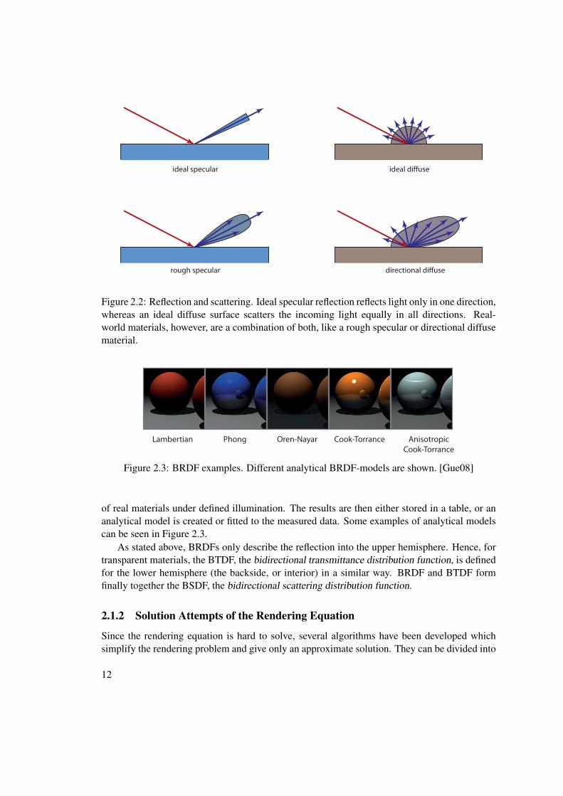
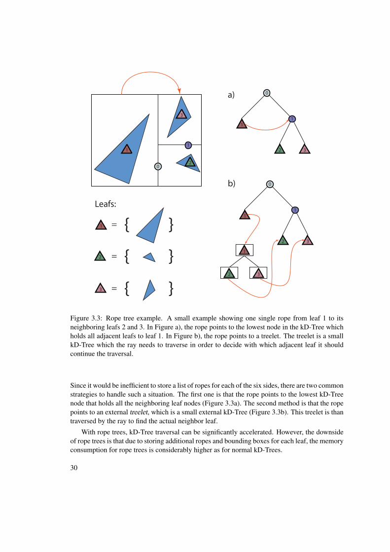
Figure 3.3: Rope tree example. A small example showing one single rope from leaf 1 to itsneighboring leafs 2 and 3. In Figure a), the rope points to the lowest node in the kD-Tree whichholds all adjacent leafs to leaf 1. In Figure b), the rope points to a treelet. The treelet is a smallkD-Tree which the ray needs to traverse in order to decide with which adjacent leaf it shouldcontinue the traversal.

Since it would be inefficient to store a list of ropes for each of the six sides, there are two commonstrategies to handle such a situation. The first one is that the rope points to the lowest kD-Treenode that holds all the neighboring leaf nodes (Figure 3.3a). The second method is that the ropepoints to an external treelet, which is a small external kD-Tree (Figure 3.3b). This treelet is thantraversed by the ray to find the actual neighbor leaf.

With rope trees, kD-Tree traversal can be significantly accelerated. However, the downsideof rope trees is that due to storing additional ropes and bounding boxes for each leaf, the memoryconsumption for rope trees is considerably higher as for normal kD-Trees.

30

3.1.4 Bounding Volume Hierarchies

Another highly efficient acceleration data structure are bounding volume hierarchies (BVH).They have been introduced by Kay and Kajia [KK86] in 1986. A bounding volume is a prefer-ably convex and geometrically simple geometric object, like a sphere or a box, tightly enclosinga usually complex object in the scene. This way it can quickly be tested if a ray intersects ormisses the original object at all. If a ray does not hit the bounding volume of an object, it can’thit the original object. Only if the ray hits the bounding volume, the ray may also hit the originalobject in the scene, and the usually much more expensive intersection test with the object of thescene has to be executed.

BVHs are hierarchies built by using such bounding volumes. Most BVHs nowadays useaxis aligned bounding boxes (AABB) as bounding volumes, because they are relatively in-expensive to test against, usually fit an arbitrary object tight enough and can easily be com-bined to hierarchies. However, spheres or oriented bounding boxes (arbitrary cuboids) are alsoused [HQL+10], albeit far less often, even if they may fit the enclosed objects tighter.

As with kD-Trees, BVHs form a tree, but in this case a tree of bounding volumes. Usuallythe arity of the nodes is two, which means that every node can have two bounding volumesas children. Both children are fully enclosed by the parent node. An arity greater than two ispossible, but hardly used in praxis.

BVHs can be constructed top-down or bottom-up. For the bottom-up way, first, some prim-itives are grouped together into a bounding volume. Then, nearby bounding volumes are com-bined to a new bounding volume. This is repeated until the whole scene is encapsulated in thehierarchy. For the top-down approach, first a bounding volume for all primitives in the sceneis built. Then, the primitives contained in the scene are divided into usually two children, eachof them again having its own bounding box. This is recursively repeated until the boundingvolumes contain only a given number of primitives. The decision where to split the boundingvolumes can be done in several ways, see Section 3.1.7.

It is important to note that the bounding volumes are not necessarily disjoint regions (seeFigure 3.4). Consider for example two nearby triangles. If they are near enough, their boundingboxes can overlap. It is an important property of BVHs that the bounding volumes may overlap.Thus, if a node has two overlapping child nodes and a ray intersects both bounding volumesof those child nodes, both of those nodes have to be tested against intersection and hence haveto be further traversed down the tree. This is the main reason why BVHs are not as efficient askD-Trees are. The big advantage, on the other hand, is that BVHs consume far less memory thankD-Trees. The maximum memory needed for a BVH is known in advance, since every primitivein the hierarchy is included exactly only once. Note that kD-Trees can have more references toprimitives in case of “cut” primitives (primitives split by a splitting plane).

Algorithmic extensions for BVHs exist to prohibit the overlapping of the nodes’ boundingvolumes by introducing spatial splits like SBVH [SFD09] or FBVH [GPP+10]. Both aim atminimizing redundant intersections tests, which results in faster traversals. The SBVH andFBVH can be considered as hybrids between BVHs and kD-Trees.

31

Figure 3.4: Overlapping BVH cells. Since BVH cells no not have to be disjoint regions, theycan overlap if the bounding box of a primitive penetrates the bounding box of another cell. If aray intersects both cells, the ray intersects the overlapping region and the primitives of both cellshave to be tested for intersection with the ray.

3.1.5 Other Common Acceleration Data Structures

Another ADS is the uniform grid. Uniform grids have the advantage of being simple and can beconstructed very fast. However, they are not optimal for non-balanced scenes. This means, if theprimitives are not evenly distributed in the scene, which is hardly the case in a general scene, therendering performance of grids can be relatively slow. This is because in some cells of the gridthere are lots of primitives to test against, whereas in other areas there are hardly any primitivesin a cell. A typical example is the “teapot in a stadium”. In this case it is hard to choose theoptimal resolution of the grid. Kalojanov et al. [KBS11a] for example have investigated the useof two-level nested grids of different solutions to remedy this.

The last presented ADS is the Octree. An Octree is basically an AABB divided into eightequally sized AABBs, which are then again recursively divided, and so on. Octrees are alsofast to construct, however, the tree of arity eight is very wide. For ray tracing, however, deeperhierarchies usually perform better because they more efficiently cut off regions of the sceneswhich are not relevant for a given ray.

A comparison of the mentioned ADS is given in Figure 3.5.

3.1.6 Divide-and-Conquer Schemes

Recently a new and quite promising approach has emerged. This approach does not need theexplicit construction of any acceleration data structure. Usually, all the acceleration structuresmentioned before have to be explicitly constructed before any ray can traverse it. If the scenegeometry changes, due to animations or the like, with a few exceptions, the whole data structurehas to be rebuilt first before starting ray traversal to render an image. One exception would be

32

a) b)

c) d)

Figure 3.5: Different acceleration data structures: a) Regular grid, b) Octree, c) Bounding Vol-ume Hierarchies and d) kD-Tree.

BVH-refitting, which however usually degrades tree quality over time and hence occasionallyneeds a complete rebuild.

To remedy rebuilding an ADS, they can be built on-the-fly. This differs from the rebuild inthe way that the ray traversal can start immediately, and the ADS is constructed while the ray tra-verses the scene. This way, fully dynamic scenes can be ray traced efficiently. Furthermore, thisapproach usually takes up far less memory then all other approaches. The on-the-fly constructedADS can basically be of any type.

The lazy construction of ADS has been already proposed in 1987 by Arvo and Kirk [AK87].Recently, Mora [Mor11b] investigated divide-and-conquer strategies for kD-Trees and Keller

33

Figure 3.6: Left: Spatial median bad case. The resulting tree hierarchy for the left cell will bemuch deeper than for the one on the right side. Right: Object median bad case. The cell onthe right encapsulates a big area of empty space. This space will be divided further and further,leading to unnecessary traversal steps.

and Wächter [AK11] as well as Áfra [Áfr12] for BVHs. Efficient algorithms and implementa-tions are subject of current and future research.

3.1.7 Splitting Strategies

The quality of some of the ADS, like kD-Trees and BVHs, strongly depends on where thesplitting planes have been placed. Several strategies for choosing the splitting positions exist.The most common ones are described below.

Spatial Median

The simplest form, and hence quite often used, is to position the split plane in the geometricmiddle of the longest axis. However, when the primitives are not evenly distributed in the scene,and in the majority of scenes this will be the case, this does not provide a very good choicefor the split, since one subtree of the node will become much deeper than the other one (seeFigure 3.6, left).

Object Median

Another easy possibility is to split at the object median. Such a split will result in half of theobjects lying on the one and the other half at the other side of the splitting plane. This canhowever lead to some geometrically unnecessarily big nodes. Consider an object consistingof many primitives in the middle of the scene, and an object with only a few primitives at thevery end of the scene. With an object median split, a node would span over primitives of thesmall object and a few primitives of the complex object, encapsulating the whole empty spacein between, which would in turn lead to unnecessary traversal steps (see Figure 3.6, right).

Surface Area Heuristic

Several other strategies for positioning the splitting planes than the ones mentioned above exist.Some of them work with heuristics. One of them has proven to be particularly useful and is used

34

frequently.To find good positions for splitting a node is crucial for an ADS to be of good quality. Good

quality for an ADS means that its traversal and intersection with a given ray is as efficient aspossible in such a way that the parts of the scene which are not pierced by the ray are culled assoon as possible.

The Surface Area Heuristic (SAH), introduced by Goldsmith in 1987 [GS87], is a heuristiccommonly used to estimate the cost of intersecting an arbitrary ray with an ADS. When con-structing an ADS, the resulting hierarchy is considered to be optimal when the cost of the SAHis minimized and hence traversing the structure with a ray is relatively fast. The SAH presumesthat the rays are uniformly distributed in the scene, that they do not stop at any primitive and thatthe ray hits the scene’s bounding box at all.

Exact SAH

Assume that a ray hits a node in any ADS and the node can be represented by any boundingbox or volume. Given that a ray hits this parent node Np, the conditional probability P of a rayhitting one of its child-nodes Nc is related to the ratio of their surface areas SA [PGSS06]:

P (Nc|Np) =SA(Nc)

SA(Np)(3.1)

The SAH is then defined as the expected cost of traversing the parent node itself and the costof intersecting the left and the right child node as shown in Equation 3.2:

C = Ct + CL P (Np|Nl) + CR P (Np|Nr), (3.2)

where C is the cost for a random ray intersecting a node, Ct is the cost for traversing thenode itself, CL and CR are the costs of traversing the left and right subtrees respectively and Nl

and Nr the left and the right nodes.The cost for the subtrees CL and CR can only be calculated when this subtrees are built. For

this reason, a greedy local approximation is used to evaluate the SAH [ZHWG08]. For this itis assumed that the children are leaf nodes and the cost of intersecting them is replaced by thecost of intersecting a primitive multiplied by the number of primitives in each of them (Equation3.3).

C = Ct + Ci nl P (Np|Nl) + Ci nr P (Np|Nr), (3.3)

where Ci is the cost for intersecting a primitive and nl and nr are the number of primitivesin the left and right child nodes respectively.

When the conditional probabilities in the above equation are expanded, the formula for theexact SAH is obtained as given in Equation 3.4.

C = Ct + Cinl SA(Nl) + nr SA(Nr)

SA(Np). (3.4)

35

Figure 3.7: Comparison of the splitting strategies (from left to right): Spatial median, objectmedian and split using the SAH.

At some point in the hierarchy construction, the cost for splitting a node will be higher thanthe cost of adding a leaf node. The cost for creating a leaf node is the cost of intersecting allprimitives in it, as shown in Equation 3.5.

CLeaf = Ci np, (3.5)

where CLeaf is the cost for making this node a leaf node and np is the number of primitivesin the node.

To create a hierarchy using SAH, the SAH must be computed for every splitting candidate.For example for kD-Trees, for every possible splitting plane the SAH cost has to be calculated.A common way to calculate the SAH is to use a sweep builder. Again, for kD-Trees, the inter-esting splitting positions are the borders of bounding boxes of the primitives. The sweep builder“sweeps” through all those candidates and calculates a value for each. The one with the minimalcost is considered the optimal splitting plane and the split is performed with it.

A comparison of the resulting splits is shown in Figure 3.7.

Binned SAH

Using a sweep builder can be expensive because usually there are many splitting candidates.Another approach is to use only a fixed number of splitting candidates which are placed onpredefined positions, so called bins. The SAH is calculated for each of the bins and the one withthe minimal cost is selected. The quality of hierarchies created using a binned SAH algorithm isonly slightly lower compared to an exact SAH [DPS10].

Binned SAH construction is used frequently for constructing ADS on the GPU, especiallyfor kD-Trees and BVHs. This is because the cost at the bins can be calculated in parallel effi-ciently. A popular method for calculating the number of primitives left and right of each splittingcandidate is min-max binning [DPS10, SSK07, PGSS06] (see Figure 3.8). Two arrays L and Hare created, both having the length of the number of bins. Each array entry corresponds to a binand is used as a counter. The entry at position i stores the events occurring between the (i−1)-thand the i-th event. In the array L, for every lower bound of a primitive, the counter at the corre-sponding position is increased. Likewise, in the array H , all the higher bounds are counted. Toget the number of primitives left and right to a splitting candidate as well as the ones intersectedby the splitting candidate, a suffix sum on L and a prefix sum on H are calculated. Having donethat, each entry (i + 1) in array L holds the number of primitives right and in array H , entryi holds the number of primitives left of a given splitting candidate. The number of intersected

36

primitives can be calculated by subtracting the number of primitives left and right from the totalnumber of primitives. With this information, SAH values for each splitting candidate can becalculated.

The resolution of the bins can either be fixed or adaptively chosen for each node, dependingon the number of primitives. Furthermore, resampling of a bin can be done. Likewise, the SAHfunction could also be evaluated first only at each n-th event and then at a finer resolution. Min-max binning can be done efficiently in parallel by using parallel primitives operations like scanand reduction. A comparison between using a sweep builder and binned SAH and their splittingcandidates is given in Figure 3.9.

Empty Space Cutoff

Finally, for large regions of empty space, an empty space cutoff is possible. Usually a thresholdfor the ratio of empty space to an axis is set. If the ratio for the empty space and the given axis isabove the threshold, the split will be placed such that the empty space is encapsulated in a singlenode.

37

1 2 3 1 0 0 1 1 2 0

0 1 1 2 1 1 1 1 1 2

11 10 8 5 4 4 4 3 2 0

0 1 2 4 5 6 7 8 9 11

L:H:

L:H:

count

sux/prex sum

Figure 3.8: Min-max binning example using 10 bins. An array entry at position i stores theevents occurring between the (i − 1)-th and the i-th event. First, the array L counts for eachentry the lower bounds of the primitives and the array H all the higher bounds. Then, a suffixsum over L and a prefix sum over H is computed. After that, in L each array entry (i + 1)holds the number of primitives completely to the right and in H entry i holds the number ofprimitives completely to the left. The number of primitives which lie partially on both sides canbe computed by subtracting the number of primitives to the left and right from the total numberof primitives. (Figure adapted from [DPS10].)

Figure 3.9: Left: SAH splitting candidates using a sweep builder. At each border of a primitive,a splitting candidate is created. Right: SAH splitting candidates using binning with 10 bins. Thesplitting candidates are created at fixed locations only.

38

3.2 CUDA

3.2.1 Motivation for General Purpose Programming on Graphics Hardware

Modern graphics cards are fully programmable, highly parallel, massively multithreaded many-core processors with tremendous computational power (Figure 3.10). Many-core processorscalculate (“render”) the graphics output pixel by pixel in many threads per processor.

Figure 3.10: Evolution of computational power of GPU and CPU [Cooc].

Early graphics cards implemented the so called fixed-function pipeline in hardware. Onlyspecific parameters could be set via a Graphics-API like OpenGL or Microsoft’s DirectX. Asgraphics hardware evolved, parts of this fixed-function pipeline were made programmable throughso-called shaders. Eventually, the graphics cards consisted of many processors, each of whichcould work independently. Since graphics cards, or graphics processing units (GPUs), havetremendous computational power, Nvidia introduced an API and programming model calledCUDA (see next Section) to use this computational power not only for graphics, but also forother calculations.

3.2.2 CUDA

CUDA [Cooa] stands for Compute Unified Device Architecture and was introduced in 2007by graphics card vendor Nvidia. CUDA is a general-purpose parallel programming model forgraphics cards. CUDA was originally only supported on Nvidia GPUs. However, Nvidia re-

39

Host Device

CUDA-Kernel

C#

C#

Figure 3.11: The host program first allocates memory on the CUDA device and copies datato the GPU. Then, it starts the CUDA kernel on the device. After the kernel has finished itscalculations, the host typically copies back the results from the device to the host.

leased their LLVM-code and now CUDA can be programmed from any language that LLVMsupports [Coob]. With CUDA, it is possible to not only render traditional graphics using raster-ization with APIs like OpenGL or Microsoft’s DirectX, but also to execute basically any othergeneral purpose code on graphics cards.

Programming Model

A CUDA program consists of two different parts. One running on the host, which is usually aCPU. The other one is executed on the device, typically a CUDA-capable GPU (Figure 3.11). Ifa graphics card contains two GPUs (“dual GPU cards”), they also contain two CUDA devices.The host program starts the device program, called a kernel. The host program also typicallyallocates memory on the device, copies data to the device, copies back results from the device tothe host and frees memory on the device. CUDA host programs are usually written in C or C++,but third party bindings for C#, Fortran or other languages exist as well.

The CUDA programming model for the host consists of two different APIs, the CUDAC/C++ API, or runtime API, and the CUDA Driver API. Both APIs can be used to manage thedevice, the (parallel) execution, the memory management, sharing of resources used by graphicsAPIs like OpenGL or DirectX, and so on. The CUDA C/C++ API is a higher-level API than theDriver API and allows for more convenient programming, while on the other hand sacrificingflexibility. A program using this API further needs a runtime DLL when executed. The C-styledDriver API, on the contrary, reveals the programmer full access to all features with the price ofhigher complexity. However, a program written for the Driver API accesses the Nvidia graphicsdriver’s API directly, hence no further DLLs are needed.

The CUDA device programs are the kernels executed on the CUDA device. They are im-plemented in CUDA device code, which is very similar to traditional C++. As of version 4.x ofthe CUDA toolchain, programming constructs like class inheritance, namespaces, templates andothers are supported.

40

Compute Capability

The CUDA Compute Capability defines the hardware capabilities of a CUDA device. Nvidiaintroduced CUDA in 2007 with the release of the G80 chip, which was used in the Geforce 8series of graphics cards. The generation of those cards featured the CUDA compute capabilityin its first version 1.0. With every revision or release of a new graphics chip, the CUDA computecapabilities were enhanced. Devices of CUDA compute capability equal or greater than 2.0 areable to handle recursive functions. The current generation of graphics cards is the 600 series(Kepler), exposing Compute Capability 3.2.

Execution Model

A CUDA kernel (a CUDA device program) is started by the host. To use the full power of theGPU, kernels are executed in parallel, one thread for one instance of a kernel. The CUDA pro-gramming model has a three-level hierarchy for arranging the parallel threads (see Figure 3.12).Threads are grouped into blocks. All blocks form the grid. The layout of the grid, i.e. how thethreads are arranged into blocks, is defined by the host program. For easier addressing with two-or three-dimensional problems, blocks and grids can be defined using two (blocks also in three)dimensions.

It is common that each thread accesses a portion of a global chunk of memory and works onthat data. For a thread to be able to access its data in the memory chunk, CUDA provides built-invariables for thread-index and block-index as well as thread-dimensions and block-dimensions.Using them, the global thread-ID can be calculated. With the thread-ID, for example an offsetcan be retrieved to access the correct data in memory.

When a kernel is started, the grid is launched. One instance of a CUDA kernel is calculatedby one single thread, which itself is part of a thread-block. If viewed from the hardware side,a CUDA device consists of several streaming multiprocessors (SM). Each of them can executeseveral blocks, but each block is executed only on a single SM.

When a grid is launched, every available SM executes a block (see Figure 3.13). Each startedthread is executed in parallel. However, the hardware executes threads in bundles called warps(see Figure 3.14). A warp consists of 32 threads. Those 32 threads run together in lockstep,which means that every one of those 32 threads has to execute the same hardware instruction.Nvidia calls this SIMT, which stands for Single Instruction, Multiple Threads (similar to thecommon term SIMD, which stands for Single Instruction Multiple Data). The lockstep furtherimplies that if one of the threads of a warp branches, all other threads have to follow that codepath even if they would not need to. To efficiently implement programs in CUDA, this issue hasto be addressed by designing appropriate parallel algorithms.

Memory Hierarchy

The CUDA architecture consists of multiple memory spaces (Figures 3.15 and 3.16). Thebiggest memory space is called the global memory. It can be accessed by all threads, andeach thread can read and write to it. To prevent threads from writing to the same location si-multaneously, atomic operations exist. However, access to the global memory is relatively slow.

41

Grid

Block (1, 1)

Thread (0, 0) ( 1 , 0) ( 2 , 0) ( 3 , 0)

(0, 1 ) ( 1 , 1 ) ( 2 , 1 ) ( 3 , 1 )

(0, 2 ) ( 1 , 2 ) ( 2 , 2 ) ( 3 , 2 )

Block (2, 1) Block ( 1 , 1) Block ( 0 , 1)

Block (2, 0 ) Block ( 1 , 0 ) Block ( 0 , 0 )

Thread

Thread Thread Thread

ThreadThreadThreadThread

Thread

Thread Thread

Figure 3.12: CUDA execution model. Parallel threads are grouped into blocks, blocks form thegrid. (Figure adapted from [Cooc])

Therefore, access patterns such that data can be efficiently cached should be used. There is alsoa memory space called constant memory, which is “read only” for a thread, but it can be readfrom faster. However, the constant memory is quite small.

Another memory space is the local memory. It is local per thread, and can be read by andwritten to only by its thread. However, this memory is not located on the chip of the SM, but inthe VRAM of the graphics card, where also the global and constant memory reside. Thus, thelocal memory is usually not significantly faster than the global memory.

In contrast, the shared memory is a memory space per block and resides on the chip ofthe SM. Consequently, the shared memory is very fast to access. Each thread of the same

42

GPU with 2 SMs

SM 1 SM 0

GPU with 4 SMs

SM 1 SM 0 SM 3 SM 2

Block 5 Block 6

Multithreaded CUDA Program

Block 0 Block 1 Block 2 Block 3

Block 4 Block 5 Block 6 B lock 7

Block 1 Block 0

Block 3 Block 2

Block 5 Block 4

Block 7 Block 6

Block 0 Block 1 Block 2 Block 3

Block 4 Block 5 Block 6 Block 7

Figure 3.13: CUDA Scalability. A multithreaded CUDA kernel consists of several blocks. Ablock is executed on a streaming multiprocessor (SM). The GPU starts as many blocks in parallelas SMs are available. (Figure adapted from [Cooc])

Warp 0

32

Warp 1

32

Warp 2

32

Warp 3

32

...

Block

Figure 3.14: CUDA Warps. The GPU executes threads in bundles of 32 threads. Those bundlesare called warps. Each thread of a warp executes the same instruction. This means, if one of thethreads branches, all other threads in this warp need to follow this branch too.

43

Texture Memory

Global Memory

Local MemoryConstant Memory

VRAM

Shared Memory

SM 0

Shared Memory

SM 1

Shared Memory

SM 2

Shared Memory

SM 3

... ...

Figure 3.15: CUDA memory hierarchy. The GPU consists of several memory areas. The VRAMholds the global, constant and local memory as well as the texture memory, which has specialaddressing modes. Each streaming multiprocessor (SM) has an on chip shared memory.

block shares the same memory (hence the name). A thread should use its own portion of thememory. To access a thread’s data, an offset needs to be calculated using the built-in thread-index variables. Shared memory is limited to 64KB on current hardware.

A memory space stemming from the graphics processing aspect of graphics cards is thetexture memory. The texture memory was initially used in computer graphics to store and accessdiverse image data. It was, however, soon used as a buffer for arbitrary data. Since a pixel in theimage data often needed to be sampled or interpolated with nearby pixels, the texture memoryhas different access patterns and is more suited for random memory access. Data residing in thetexture memory can be accessed in constant time, whereas for the other memory areas the accesstime depends on alignment of the memory access pattern and therefore on the cache efficiency.

When designing an algorithm for CUDA, it is therefore beneficial to consider the diversememory spaces.

Graphics Resources Sharing

When programming computer graphics applications, data like vertex positions, textures andsuch, have to be managed. Usually, graphics APIs like OpenGL or DirectX are used. Thementioned graphics resources are passed to that API such that the graphics card can use those

44

A B A can write to B

A B A can read from B

(Per Thread) Local Memory

(Per Block) Shared Memory

Global M

emory

Constant Mem

ory

Texture Memory

Host

Thread (Device)

Figure 3.16: Memory access. The host and the threads from the device can read and write fromand to different memory locations. The only memory where both can read from and write to isthe global memory. Hence, data exchange is usually handled via this memory.

resources to render images. These resources then reside in the memory of the graphics card.When using CUDA in a graphics application, it is often the case that the CUDA kernels need toaccess the graphics data, e.g. to modify vertex positions for animations. It would be inefficientto copy the data of the graphics resources into CUDA buffers, modify them, and copy the databack to the graphics resources. Therefore, the CUDA API provides possibilities to share thegraphics resources of OpenGL or DirectX, read and write to them directly without having tocopy the data back and forth. In terms of a CUDA ray tracer this is important, since the CUDAray tracing kernel can directly write into the frame buffer of the graphics API, which is thendirectly displayed by the application using the graphics API.

Compilation and Tools

The CUDA device code is programmed in *.cu-files. If the CUDA host code is written in Cor C++ and the C/C++ API is used, those files must also have this extension. Host and devicecode can exist together in the same .cu-file. The Nvidia Cuda Compiler (nvcc) then compiles thecode. The compiler first extracts and compiles the device code and then uses the native C/C++

45

compiler to compile the host code.The device code can be compiled to *.cubin binary files which can be executed immediately.

A binary file however is compiled only for a specific graphics chip. So, in order to be able torun the same device code on multiple versions of graphics chips, like on a GeForce 200 and aGeForce 600, two separate binaries would have to be generated and the appropriate one has tobe loaded at runtime.

The other way to compile CUDA device code is to compile to PTX format. PTX is anassembly-like intermediate language, used by Nvidia’s graphics cards. The PTX-files can thenbe loaded and automatically just-in-time (JIT) compiled by the graphics driver for the currentgraphics chip on which the code needs to be executed on. Since this JIT-compilation can takesome time, the JIT-compiled code is temporarily stored by the graphics driver. Only when a newversion of the PTX exists, the JIT-compilation is performed again.

For debugging CUDA device code, Nvidia released a debugging tool called Nsight. Nsightis available as a plug-in for Microsoft’s Visual Studio and Eclipse. With the help of the plug-in itis possible to debug CUDA device code almost like CPU code, which means setting breakpoints,stepping through code as well as variable inspection. Without Nsight, these debugging featuresfor CUDA device code are not possible and debugging can only be done by looking at the dataresults calculated by a CUDA kernel. Furthermore, Nsight also provides a profiler so investigatewhat parts of the code consume the most time or bandwidth.

CUDA and C#

The host languages supported by Nvidia for programming CUDA are C and C++. Both APIs,the runtime and driver API, are C or C++ APIs. To use the features of CUDA in another pro-gramming language, one has to gain access to those APIs first. In case of C#, which was usedas the host language in this thesis (see Chapter 5), the freely available runtime library calledCUDA.NET was used to gain access to the APIs. The CUDA.NET library itself performs un-safe calls to C/C++ methods from the CUDA APIs. More details on accessing CUDA in C# aregiven in the section on the implementation.

3.2.3 CUDA and OpenCL

OpenCL is an open industry standard which also allows for parallel general-purpose program-ming on supported devices. Supported devices include diverse CPUs (Intel, AMD and Cellarchitectures), GPUs (Nvidia, AMD and Intel), as well as ARM-processors for cell-phones.OpenCL offers roughly the same features as CUDA, but is not limited to only Nvidia graphicscards.

However, at the time of the beginning of the implementation for this thesis, OpenCL wasin an early state and some limitations existed concerning memory management and efficientsharing of graphics resources. Also, some of the needed SDKs had not been released, or wereonly in beta-phase. On the contrary, Nvidia provided an online platform with helpful resourcesfor CUDA-programming and announced the debugging tool Nsight. Moreover, Nvidia’s CUDAhas always been ahead of the OpenCL specification, so it has been possible to use the latestfeatures available on graphics cards. It is most likely that this will continue in the future. Based

46

on the support for CUDA from Nvidia in terms of online resources and tools as well as of thepower and possibilities of the language, it was finally decided to use CUDA for this thesis.

47

CHAPTER 4Ray Tracing on the GPU

This chapter first gives an overview of the most important steps towards real-time ray tracing.After that, as a contribution, we present a canonical iterative version of the ray tracing algorithm.It has been derived from several collected publications. Building on that algorithm, furthermorea parallel version is given. Later on, the section on “KD-Trees for GPUs” describes the mainmethods for implementing and traversing kD-Trees on GPUs. Finally, the last section presentsour new data structure, the Über-kD-Tree.

4.1 Advent of Real-Time Ray Tracing

One of the very first attempts to make ray tracing work in real-time was done by Muuss [MM95]in 1995 from the U.S. Army Research Laboratory for the development of missile automatictarget recognition. He used an array of 8 network computer with 12 CPUs each to render 5NTCS-frames per second. A few years later, in 1999, Parker et al. [PMS+99] used a supercom-puter with up to 64 cores to render ray-traced images with a resolution of 600x800 in real-time.In 2001, Wald et al. [WSBW01] first developed a highly optimized ray tracer for the CPU,which could render images at interactive frame rates. Later the same year, they also released aversion for network distributed rendering [WSB01]. Finally, in 2002 Purcell et al. [PBMH02]mapped ray tracing to the back then newly programmable rendering pipeline on GPUs. At thattime, the vertex- and the fragment-stage of the former so-called fixed-function pipeline becameprogrammable. Purcell et al. implemented a ray tracer using the fragment shader.

Besides research for ray tracing in real-time on CPU and on GPU, some attempts have beenmade to build custom hardware for ray tracing acceleration. In 2004, Schmittler et al. [SWW+04]presented SaarCOR, an FPGA-chip for accelerating dynamic scenes. One year later, Woopand Schmittler [WS05] developed the RPU, the “Ray Processing Unit”. In 2006, Woop etal. [WMS06] released the DynRT -architecture using B-kD-Trees, a hybrid data structure ofBVHs and kD-Trees. Also, commercial attempts have been made for custom hardware, like theCausticOne by Caustic Graphics, Inc. [CG] in 2010.

49

During the last decade, however, graphics cards have reached a high level of computationalpower, and researchers have tried to utilize this power as it became available. One of the firstattempts to ray tracing on the GPU using kD-Trees was made by Foley in 2005 [FS05]. Theypresented two new traversal methods for traversing kD-Trees on the GPU, the kd-restart (Sec-tion 4.4.2) and the kd-backtrack algorithms (Section 4.4.3). The two algorithms do not need astack, which was back then very expensive to use on the GPU.

Acceleration data structures are crucial for fast ray tracing. Therefore, Popov et al. [PGSS06]as well as Wald and Havran [WH06] investigated methods on how to build good quality kD-Trees and how to build them fast. In the same year, Woop et al. [WMS06] presented the B-kD-Tree (bounded kD-Tree). The B-kD-Tree stores two splitting planes for each node, instead ofone, like for normal kD-Trees. Wächter and Keller [WK06] developed the Bounding IntervalHierarchy (BIH). The BIH is basically a kD-Tree with object partitioning. For each level, itstores also two splitting planes. They furthermore use a new global heuristic for setting thelocations of the splitting planes.

In 2007, Popov et al. [SPS07] released an improved version of the kD-restart algorithmwhich uses ropes (Section 3.1.3) and packet traversal (Section 2.3.2). At the same time, Horn etal. [HSHH07] improved the kd-restart algorithm by adding a short stack (Section 4.4.4). Also in2007, Shevtsov et al. [SSK07] presented an interactive ray-tracing algorithm for the CPU. Theyalso used kD-Trees and the algorithm scales linearly to available CPUs.

Zhou et al. [ZHWG08] presented a real-time ray tracer in 2008. It runs completely on theGPU and rebuilds the kD-Tree every frame, which allows arbitrary animations. In the same year,Bikker presented his Arauna CPU real-time ray tracer [Bik11]. It is written in highly optimizedC/C++ code and uses different BVHs for static and dynamic parts of the scene.

Up until 2009, the main bottle-neck for GPU ray tracing programs where thought to be thelimited memory bandwidth. However, Ailia and Laine from Nvidia showed in 2009 [AL09]that the main limiting factor, before memory bandwidth takes any effect, is the under-utilizationof the GPU and the performance penalty for branching code. They released a follow-up paperin 2012 for current Nvidia graphics cards [ALK12]. In 2009, Stich et al. [SFD09] presentedthe SBVH, the spatial-split BVH. In this data structure, they allow that also spatial splits canbe made when constructing the BVH in addition to the conventional object partitioning. Thus,costly overlapping of cells can be reduced. Popov et al. [PGDS09] presented a similar work,where they investigate different possibilities for spatial splits for BVHs.

In 2010, Pantaleoni and Luebke, also from Nvidia, presented their HLBVH algorithm [PL10],which allows real-time ray tracing of fully dynamical scenes by constructing the BVH fromscratch every frame. The HLBVH is a BVH which uses the Z-Morton curve [Mor66] to sortand cluster the primitives in a scene, and then emits the hierarchy based on this sorted order. Inthe same year, Danilewski et al. [DPS10] presented their real-time ray tracer for fully dynamicscenes using kD-Trees which are rebuilt every frame. They used a binned SAH kD-Tree builderand implemented several so-called stages to fully utilize the computational power of the GPUfor processing different tree-levels. Also in 2010, Nvidia introduced OptiX [PBD+10]. OptiX isa programmable ray-tracing system which allows developers to develop their own real-time raytracing application. Currently OptiX uses HLBVH internally.

In 2011, Garanzha et al. [GPM11] improved the HLBVH algorithm by using work queues

50

instead of the compress-sort-decompress scheme [GL10] used in the original algorithm. Besidesthe dominance of kD-Trees and BVHs on current real-time ray-tracing research, Kalojanov etal. [KBS11b] showed that using a two-level uniform grid can be especially useful for dynamicscenes, where fast rebuilding of the data structure for each frame is important. Moreover, Wu etal. [WZL11] showed how to build kD-Trees using SAH entirely on the GPU.

Also in 2011, a new category of ray-tracing algorithms has been introduced, the so-calleddivide-and-conquer ray tracing (DACRT) (Section 3.1.6). DACRT does not need an explicitlystored acceleration data structure like a BVH or kD-Tree, but subdivides the scene on-the-flywhen tracing rays. Mora’s DACRT algorithm [Mor11b] is a CPU implementation and uses a kD-Tree-like spatial subdivision scheme which he called axis-aligned spatial subdivision (AASS).He also introduced the direct-trace library [Mor11a], which is a ray-tracing library which usesDACRT. It supports CPUs as well as GPU acceleration. Recently, Keller and Wächter [AK11]and Áfra [Áfr12] presented DACRT algorithms using a BVH-like approach instead of the AASS.

Our implementation of the traversal of the kD-Tree is similar to the method used in Zhouet al. [ZHWG08]. It is a stack-based traversal with a stack per ray. This type of traversal isdescribed in Section 4.4.1. As far as kD-Tree construction is concerned, we use the constructionalgorithm on the CPU which was already implemented in Aardvark and convert the resultingkD-Trees to a format suitable for the GPU.

In the following, the adaption of the basic ray tracing algorithm, introduced in Section 2.3,for efficient implementation on the GPU will be described as well as variants of kD-Trees forGPUs.

4.2 Iterative Ray Tracing

On GPUs, recursion was not supported until recently and still, recursion is inefficient on GPUs.Therefore, we present a canonical iterative ray-tracing algorithm that we derived from variousinformation collected from a number of publications. The iterative algorithm of the basic raytracing algorithm (Algorithm 1) is shown in Algorithm 3. Note that only the Trace()-functionchanges, as it is now implemented iteratively. All the other functions remain the same as inAlgorithm 1.

The iterative version has to make use of a stack to store the rays to be traced. With the givenpseudo-code in Algorithm 3, the ray tree (c.f. Section 2.3.2) is traversed in a depth-first, left-firstmanner. If the tracing of reflection rays is done, the refraction rays are traced. If they againcreate new reflection rays, they are first traced again until the stack of rays is empty.

4.3 Parallel Ray Tracing

The parallel version of the basic ray tracing algorithm is the same as Algorithm 1, with the ex-ception that the for each-loop in line 2 in theDoRayTracing()-method is executed in parallel.Since the calculations for a pixel are independent of other pixels, as many pixels as possible canbe calculated in parallel. Therefore, an own thread is started for each pixel and its primary ray.The primary ray and its secondary rays are traced independently of the other pixels. When all

51

Algorithm 3 Iterative Trace()-function

1: function TRACE(primRay)2: color ← black3: ray ← primRay4: refraction stack ← new ray stack → stack for refraction rays5: depth stack ← new int stack → stack for storing recursion level6: tree depth← 07: continueLoop← true8:

9: while continueLoop do10: hit← INTERSECT(ray, scene)11:

12: if hit then13: color += SHADE(ray, hitPoint)14: tree depth← tree depth + 115: if Material is reflective and tree depth <= maximum tree depth then16: if Material is transparent and not total internal reflection then17: refractionstack.PUSH()← RAY(hitPoint, refracted(ray.direction))18: depth stack.PUSH()← tree depth19: end if20: ray ← RAY(hitPoint, reflected(ray.direction))21: else → Diffuse Material22: continueLoop← false23: end if24: else → no hit25: color += BackgroundColor26: continueLoop← false27: end if28:

29: if not continueLoop and stacks not empty then30: ray ← refraction stack.POP()31: tree depth← depth stack.POP()32: continueLoop← true33: end if34: end while35: return color36: end function

52

calculations for a pixel have been done, the calculations for the next pixel which has not yet beencalculated can be started.

On CPUs, multiple threads can be used to parallelize the algorithm, and SIMD and packettraversal (Section 2.3.2) can be used as optimizations to gain performance. On GPUs, severalhundreds of threads are started in parallel. The limits of parallel execution are determined by thewarps and block sizes.

4.4 KD-Trees for GPUs

4.4.1 Stack-based Iterative Traversal

On GPUs, recursive traversal is nowadays possible in principle, however it is comparably slow.Therefore, an iterative traversal is favored. In this case, one way for traversing a kD-Tree is tomaintain a stack.

Algorithm 4 shows the iterative version of the IntersectNode() function. All other func-tions remain the same as in Algorithm 2. The main loop is the outer while-loop. It can only bebroken when a leaf found an intersection or if the traversal did not find any intersection at all,meaning that all paths have already been traversed, i.e., that the stack is empty. This is similarto the recursive variant, when there are no more recursive calls left. The while-loop for the leafis necessary because if a node is popped from the stack, the new node can be a leaf again. Whentraversing an inner node, there are still the three following cases. The ray can be on the left orright side of the splitting plane, or crossing it. In the former two cases, just the new node is setand the loop is continued. Only when the ray crosses the splitting plane, the node further awayis pushed onto the stack and the traversal continues with the nearer one. Since the nodes arepushed on the stack and are later possibly retrieved again, this leads to the same traversal stepsas with the recursive variant.

Maintaining a stack for each ray on the GPU was inefficient on graphics cards before therelease of Nvidia’s Fermi-architecture in 2010. With Fermi, a conventional cache hierarchy formemory access was introduced [Coo10]. Furthermore, there had been an overall speedup, suchthat the implementation of stacks became feasible. Therefore, prior to this architecture, traversalmethods have been invented which did not need a stack. They will be described in the nextsections.

4.4.2 KD-Restart

In 2005, Foley and Sugerman [FS05] released the first two algorithms for traversing a kD-Treeon graphics cards. Back then, recursion was not supported on graphics hardware at all, andusing a stack for traversing a kD-Tree on the GPU was inefficient. Therefore, they developedtwo stackless traversal methods.

The first one is the kD-Restart algorithm. Instead of maintaining a stack for a ray, theyonly keep its values for tmin and tmax, the minimum and maximum t-values for the ray (seeFigure 4.1 left). Then, when a leaf is tested for intersection with the ray but the ray does nothit any primitive in it, the traversal with this ray is restarted from the root with new values fortmin and tmax. The new tmin is set to the former tmax and the new tmax is set to the border of

53

Algorithm 4 Iterative IntersectNode()-function maintaining a stack

1: function INTERSECTNODE(node, ray)2: stack ← new stack3: while true do4: while node is leaf do5: foundHit← INTERSECTLEAF(node, ray)6: if foundHit then return foundHit7: else8: if stack not empty then node← stack.POP()9: else return no intersection

10: end if11: end if12: end while13:

14: if ray on left of node’s splitting plane then15: node← node.ChildLeft16: end if17: if ray on right of node’s splitting plane then18: node← node.ChildRight19: end if20: if ray crosses node’s splitting plane then21: if node.ChildLeft is nearer than node.ChildRight then22: stack.PUSH()← node.ChildRight23: node← node.ChildLeft24: else25: stack.PUSH()← node.ChildLeft26: node← node.ChildRight27: end if28: end if29: end while30: end function

the scene. This way, the traversal will take its path to the nodes that would usually have to bepushed on the stack. However, due to the re-traversal of the data structure, kD-restart leads toredundant traversal steps.

Popov et al. [SPS07] presented an improved version of the kD-restart algorithm by addingropes to the leafs of the kD-Tree. These ropes are links to the neighboring cells of the leaf(see Section 3.1.3). When intersecting a leaf does not result in an intersection, the rope to theneighbor cell is followed and the leaf cell or cells pointed to are tested. This way, the redundanttraversals are eliminated, but at the cost of higher memory usage for the ropes. Popov et al.further used packet traversal (Section 2.3.2) to exploit ray coherence.

54

→ →

Figure 4.1: Left: KD-Restart. When the ray traversal unsuccessfully tested a leaf for inter-section, the ray traversal is restarted from the root with new values for tmin and tmax. Right:KD-Backtrack. When the ray traversal unsuccessfully tested a leaf for intersection, a “back-track” traversal is started, until the node is found which would have been pushed on a stack, andtraversal continues from there. (Figures adapted from [FS05].)

4.4.3 KD-Backtrack

The second stackless kD-Tree traversal presented by Foley in 2005 [FS05] is the kD-backtrackalgorithm. They already noticed that the kD-restart algorithm needs lots of redundant traversalsteps. To remedy this, they added a parent link to each node. This way, when a leaf is tested forintersection with a ray but the ray does not hit any primitive in it, the traversal is “back tracked”.This means that they look for the lowest parent node in the leaf’s ancestors which intersectsthe appropriate tmin and tmax values (Figure 4.1, right). When this node is found, the normal“down traversal” continues from this ancestor node. As in the improved kD-restart version byPopov et al. [SPS07], the kD-backtrack needs more memory because the parent links as well asthe bounding boxes for each node have to be stored.

4.4.4 Short-Stack and Push-Down

Another stackless algorithm was published by Horn et al. in 2007 [HSHH07]. They also builttheir algorithm on kD-restart, but added a short, fixed-sized stack where nodes can be pushedand popped as usual. Whenever a stack underflow occurs, the algorithm reverts to the standardbehavior of the kD-restart algorithm. In case of an overflow, the deepest node in the stack isdiscarded.

They also added push down. In the kD-restart algorithm, the traversal of the data structureis restarted always at the root. Horn et al. observed that they could push the entry node for therestart down the tree hierarchy, as long as the ray does not cross the splitting plane. Hence, theysave unnecessary traversal steps when restarting the traversal.

Horn et al. already observed in their implementation the main limiting factors for ray tracingon the GPU: the parallel workload is not distributed equally, the memory latency and last but notleast, the penalty payed for divergent code.

55

a) b) c)

Figure 4.2: Über-kD-Tree. a) Some objects in the scene. b) Objects with their Object-kD-Trees.c) The Über-kD-Tree (red) is a kD-Tree over the Object-kD-Trees.

4.5 Über-kD-Tree

In this thesis, we developed a new data structure which we call the Über-kD-Tree. It is a kD-Tree which consists of kD-Trees in its leaves. The kD-Trees for the leaves are kD-Trees pergeometrical object and we call them Object-kD-Trees. Figure 4.2 shows the idea of the Über-kD-Tree.

The main reason why we wanted to do implement such a data structure is to interactivelyadd and delete objects to the scene without having to deal with major data structure rebuilds.This way, only the Über-kD-Tree needs to be rebuilt, which can be done quite fast. Furthermore,when there are only a few objects in a scene, a list of those Object-kD-Trees is sufficiently fast.However, for lots of objects, having a kD-Tree over the Object-kD-Trees to cull objects can bebeneficial. Shevtsov et al. [SSK07] mentioned that they experimented with two-level kD-Treesand reported a speedup when using this data structure with four or more non-overlapping objects.

To traverse the Über-kD-Tree, first the Über-kD-Tree is traversed. If a ray hits a leaf whichcontains an Object-kD-Tree, this Object-kD-Tree is traversed to find an intersection of the raywith the geometry.

Both, the Object-kD-Tree and the Über-kD-Tree are implemented in the CUDA ray tracerfor this thesis (see Chapter 6 and Section 6.4). Results using the Über-kD-Tree will be presentedin Section 7.3.

56

CHAPTER 5CUDA Library

This chapter takes a closer look at the CUDA library which has been developed for the VRVis-internal rendering engine Aardvark. First, the host side, including context and memory manage-ment as well as data-types, is presented. Later on, an overview of the device side of the libraryis given.

5.1 Overview

CUDA is by default only accessible from C or C++ (see Section 3.2.2). To access CUDAfunctionality from within C#, the function-calls to the CUDA-APIs have to be wrapped. Sincethe CUDA-API is already very large, this would be a lot of work to do manually. Fortunately,there is a library for C# called CUDA.NET [GAS] which is freely available. CUDA.NET wrapsthe function calls of the CUDA-API 3.0 in both versions, the runtime API and the driver API.However, the CUDA-API and hence the wrapped functions are very low-level. To make workingwith CUDA convenient in terms of object orientedness, it is useful to implement a higher-levellibrary on top of the low-level API. Besides that, as mentioned above, the CUDA.NET libraryin its current version wraps the CUDA-API version 3.0. The CUDA-API version current duringthe main programming tasks for the thesis was 4.2. Since the API partially changed, some ofthose new API functions were wrapped manually to access new functionality.

After several iterations, the final implementation of the CUDA library CUDALib supportsbuilt-in data types, ready to use within Aardvark and C#, as well as semi-automatic memory-management for the GPU.

The CUDALib is separated in two parts, the host side and the device side (Figure 5.1). Thehost side part contains the management code for CUDA, hence, the C# code. The part of thedevice side contains CUDA device code which can be used from within any CUDA kernel. Also,the ray tracer described in Chapter 6 is now part of the library, such that the ray tracer can beused from within any Aardvark application.

57

Device

Math Utilities

Aardvark.CUDA.Lib (Host)

Base DataTypes Graphics

Figure 5.1: The CUDALib host and device parts. The host part has its root-namespace inAardvark.CUDA.Lib with sub-namespaces: Base, which includes all the main-functionality likeCUDA-Context, -Device, -Module and -Function management, as well as device memory man-agement, namespace DataTypes, which provides read-to-use data structures for working withCUDA, and finally the namespace Graphics, which provides data types for graphics resourcesharing. The device part has no particular namespace, but is logically subdivided into Math,which includes vector-, color- and matrix-classes, and some utility-functions bundled in Utili-ties.

5.2 Host Side

The host side is the main part of the CUDA library. It provides a high-level abstraction of theCUDA-API in C#. The library is integrated tightly into Aardvark and can be used from any ofAardvark’s research-projects to gain access to the GPU-computing power of graphics cards.

5.2.1 Management

Context Creation

On the host side, the main object is the CudaContext (Figure 5.2), which encapsulates the CUDAcontext in a very convenient way. When a new CudaContext is created, it first selects the CUDA-device automatically if no preferred device is specified. Then the CUDA-context is created onthis device with the given flags, like graphics resource sharing or others. Also, a new memorymanager is created, which will be described below.

When context creation is done, one or more CUDA-modules, which are the PTX-files, canbe loaded. Modules can also be created by run-time compiling CUDA source-code, which canbe passed as a simple C#-string to the CUDA-runtime compiler. This CUDA-runtime compilerwas developed in collaboration with Georg Haaser at the VRVis Research Center and is anencapsulation of the Nvidia CUDA-compiler nvcc. It translates our custom defined compiler-switches to actual ones for nvcc and then calls it with the translated commands. This way wecan compile CUDA-code during the runtime of a C#-program. The advantage is that the CUDA-device code can be customized to specific needs of the currently running environment.

After the CUDA-modules are loaded, the functions, i.e. the CUDA-kernels, can be loadedfrom the modules. The layout of the grid, which arranges the threads into blocks, is done perfunction. In the current implementation, one CUDA-context per CUDA-device is supported.Since a CUDA-context can be shared among CPU-threads, more than one CUDA-context is

58

CudaContext

CudaModule

CudaFunction

IRenderer CudaDevice

CUDA.NET

CudaDotNet

DoubleSidedDictionary

CudaMemoryManager

Figure 5.2: The CudaContext is the central part of the CUDALib. It contains and managesthe CudaDevice, the loaded CudaModules, the CudaMemoryManager for managing device-memory and, if sharing of graphics resources is needed, also a concrete Aardvark-Renderer.

not necessary. However, if a system has more than one CUDA-capable device, the support ofmultiple devices is important and therefore supported by the library.

Memory Management

The CUDALib furthermore has its own GPU memory manager, the CudaMemoryManager. Thememory manager maintains a mapping from C#-(CPU-)objects to GPU-“objects”. It does this bystoring the references from C#-objects to the actual memory addresses on the GPU. To maintainthis mapping, aDoubleSidedDictionary〈S,D〉 has been implemented. It is a dictionary whichcan look up two values 〈S,D〉 (source and destination, respectively) fast by storing them as key-value-pairs in two normal C#-dictionaries, but one time with 〈S,D〉 as key-value-pair and onetime reversed as 〈D,S〉.

For the memory manager, the double-dictionary is created as DoubleSidedDictionary〈IntP tr, object〉. The IntP tr are the pointers to the GPU memory location, thus, the addressof an object in GPU-memory. The object is the reference to a normal C#-object.

When a new C#-object is added to the memory manager, the C#-object reference is addedto the dictionary. One can register the C#-object in the memory manager first without copyingit to the GPU, and copy it to the GPU later. In this case, a “virtual” pointer for the GPU-addressis created, which is replaced by the actual one later. To copy a C#-object to the GPU, it isfirst pinned so that its address can be taken. Pinning in C#-terms means, that an object is fixedto its current memory location and the .NET-runtime can not move it as long as it is pinned.The object is then copied to the GPU and the returned memory address is stored as an IntP trtogether with the reference to the C#-object in the dictionary. Finally, the C#-object does notneed to stay pinned anymore and is unpinned again. When an object is copied back from theGPU, the GPU-memory location is looked-up in the dictionary and the corresponding data isdownloaded from the GPU.

When it comes to a scene hierarchy with lots of geometric objects which may share texturesor material properties, the same C#-object could be registered several times. To prevent load-ing the same object to the GPU more than once, the memory manager implements a referencecounting approach. Therefore, when an object is added to the memory manager, it first checks ifthe object has been registered already with this memory manager. If so, only a reference-count

59

to this object in the memory manager is increased and the current GPU-handle is returned. Ifthe object is not already registered with the manager, it is added. Likewise, the reference countis decreased when a C#-object is unregistered from the manager. If the reference count becomeszero, the memory for the object on the GPU is freed. An example using the memory manager isshown in Listing 5.1.

In C#, besides arrays, structs provide the correct data-layout for working with CUDA. How-ever, they are value types in C# and therefore no pointer to them can be maintained. After severalattempts we came up with an elegant solution. To prevent writing a wrapper-class for each struct,any struct was encapsulated into an array of length 1. This way, the memory manager could alsokeep track of the mapping between C#-structs and their CUDA-representation. This is, however,not an integrated feature of the library itself, but rather a direction on how to use structs withthe library, such that data changes in structs are visible for the memory manager. An example isshown in Listing 5.2.

The memory manager provides a convenient way to manage memory on the GPU. CPU-objects are registered first, can then be loaded to the GPU automatically or manually, updatedif necessary and unregistered if not needed anymore. Currently the library supports only C#-structs and arrays of such to be managed by the memory manager due to the memory-layout ofstructs in C#. Support for classes could optionally be implemented.

Kernel Launch

Besides the memory management, one of the most convenient features of the library is thatCUDA-kernels can be launched as easy as normal C#-functions. Kernel launches with the use ofour library are simply of the form myKernel.Call(...myParameterList...) (see Listing 5.1).Call() is a C#-function with a variable parameter list. The passed parameters are checked bythe memory manager if one of them is registered in it. If so, the stored GPU-address is passedas parameter to the kernel. Otherwise, the data is copied to the GPU. The passed parameters arefurthermore automatically correctly aligned.

Without this convenient kernel-call, the parameters would have to be mapped manually, theactual program code would get much longer and therefore prone to errors.

Other Features

The library also supports other important CUDA-features. The CUDALib is implemented insuch a way that it completely supports CUDA-streams. Modern CUDA-capable GPUs can rundifferent CUDA-kernels in parallel, as well as executing CPU↔GPU memory transfer for onekernel in background when the GPU is concurrently executing another kernel. Per default, allkernels and memory transfers belong to stream 0. When using different streams for differentkernels and their associated memory transfers, those kernels can be executed either interleavedor in parallel, and their memory transfers can be hidden by running in the background.

Furthermore, CUDA exposes a timer to measure the runtime of GPU operations. This timerworks a little different than conventional CPU timers. The CUDA-timer works with events. Touse the timer, a start event is created and inserted into the GPU-instructions. When then theevent is passed, or “executed”, the current time is recorded. Similarly, a stop event is created

60

var cudaContext = CudaContext.Create();var cudaModule = cudaContext.LoadModule("myCUDAModule");var cudaKernel = cudaModule.LoadFunction("myCUDAFunction");

// retrieve the memory managervar cmm = CudaContext.CudaMemoryManager;

// create some C#-object. Let’s create an array of floats:var myObj = new float[] 0.0f, 1.7f, 3.0f ;

// register the object in the memory managercmm.Register(myObj);

// copy myObj-data to GPUcmm.ToDevice(myObj);

// do something, like starting a CUDA-kernel:// set grid-layout first// (needs to be done only once per kernel)cudaKernel.SetKernelLaunchLayout(myKernelLayout);

// then launch kernelcudaKernel.Call(myObj /* ...other kernel parameters... */);

// after kernel has finished,// copy myObj-data back from GPUmyObj = cmm.FromDevice<float[]>(myObj);

// unregister from memory manager if myObj not needed anymorecmm.Unregister(myObj);

Listing 5.1: CUDALib example memory manager and kernel launch. First, a CUDA-context iscreated and a module including a function is loaded. After that, a reference to the CudaMemory-Manager is retrieved. Then some C#-object is created and is registered in the memory manager.When copying the data to the GPU, the “virtual” pointer created by default in the memory man-ager is replaced by the actual one. Next, the kernel launch layout ist set and the CUDA-kernelis called. Finally, when the kernel has finished, the data is copied back and, if the data is notneeded anymore, unregistered from the memory manager. If there are no more references tomyObj, its data on the GPU is deleted and the corresponding memory freed.

61

// define some C#-struct for demonstrationstruct MyStruct

public int a;public int b;

// create a struct and fill it with datavar str = new MyStruct();str.a = 17;str.b = 29;

// create an array of length 1 which contains the structvar structArray = new MyStruct[1] str ;

// create CUDA-context, load module and functionvar cudaContext = CudaContext.Create();var cudaModule = cudaContext.LoadModule("myCUDAModule");var cudaKernel = cudaModule.LoadFunction("myCUDAFunction");

// retrieve the memory managervar cmm = CudaContext.CudaMemoryManager;

// register the object in the memory managercmm.Register(structArray);

// change some data in the structstructArray[0].a = 333;

// copy the data to GPU. The changed value for// structArray[0].a will be visible on the GPU!cmm.ToDevice(structArray);

// set grid-layoutcudaKernel.SetKernelLaunchLayout(myKernelLayout);

// launch kernelcudaKernel.Call(structArray /* ...other kernel parameters... */);

// copy the data back from GPUstructArray = cmm.FromDevice<MyStruct[]>(structArray);

// unregister from memory manager if data not needed anymorecmm.Unregister(structArray);

Listing 5.2: CUDALib example on how to encapsulate structs in arrays. For demonstrationpurpose, first, a struct needs to be defined, constructed and filled with some data. After that, thestruct is encapsulated into an array of length one. This way, changes of the data of the struct arevisible to the memory manager and hence later on transfered to the GPU. The remainder of thisexample is similar to Listing 5.1.

62

var cudaContext = CudaContext.Create();var cudaModule = cudaContext.LoadModule("myCUDAModule");var cudaKernel = cudaModule.LoadFunction("myCUDAFunction");

// create an C#-array of floatsvar floatArray = new float[] 0.0f, 1.7f, 3.0f ;

// create a CudaArray from itvar cudaArray = new CudaArray<float>(floatArray, cudaContext);

// CudaArrays can be worked with as normal C#-arrayscudaArray[1] = 2.0f;

// copy data to GPUcudaArray.ToCudaDevice();

// set grid-layoutcudaKernel.SetKernelLaunchLayout(myKernelLayout);

// launch kernelcudaKernel.Call(cudaArray /* ...other kernel parameters... */ );

// copy data back from GPUcudaArray.FromCudaDevice();

Listing 5.3: CUDALib CudaArray example. This listing shows the same example as Listing 5.1,but using a CudaArray instead of manually registering a C#-array in the CudaMemoryManager.CudaArrays can be worked with as normal arrays in C#.

and inserted where the stop time should be recorded, for example after the memory transfersand kernel execution. CUDA can then provide the elapsed time between the start and stopevents. Since memory transfers and kernel launches can run asynchronously, measuring timewith CPU timers may report incorrect timings and hence CUDA-timers should be used in thatcase. Furthermore it should be noted that the stop event mentioned above is recorded only whenit is actually executed. For this reason, before the elapsed time can be read from the CUDA-timers, one has to make sure that the events have been recorded already. This is simply done bya CUDA-synchronize instruction for the stop event. The synchronize instruction tells CUDA toexecute all GPU code until the given event. After that it is guaranteed that the events have beenrecorded and the correct elapsed time can be read. All this synchronization is done automaticallyby the library, or, if required, it can be performed manually as well.

5.2.2 Built-In Data-Types

When programming with CUDA, one observes that certain CUDA-internal data types are usedquite frequently, but are cumbersome to use especially from within C#. That is why four spe-cial data types have been implemented in the CUDALib. They can be seen as two groups ofdata types: arrays, containing homogeneous data, and a composite data structure, containing

63

heterogeneous data.A conventional array on the GPU is provided by the CUDALib as the CudaArray〈T 〉,

which contains elements of type T . They can be worked with as usual C#-arrays, can be used askernel-parameters and can be conveniently loaded from and to the GPU. Listing 5.3 shows thesame code-example of Listing 5.1 with the use of a CudaArray.

A similar purpose to the CudaArray is fulfilled by the CudaPageLockedArray〈T 〉 oftype T . The difference is that the data in the RAM can not be paged anymore when page-locked,or pinned. Such arrays can additionally be mapped into the GPU memory space. Page-lockedarrays allow very fast updates, however, since using them reduces overall physical memoryfor the operating system, they should be used sparingly. The last array data structure is theCudaTexture. The CudaTexture is a 1D, 2D or 3D array which is internally mapped to theCUDA-internal CUDAArray. It provides all functionality expected for textures, like borderwrapping or clamping, filtering, normalized coordinates and so on.

Besides the array data structures, it is often required to have objects with heterogeneousdata. For this reason, the CudaStruct〈T 〉 was implemented, where T can be any C#-struct.This way, the library also permits to work with heterogeneous data with CUDA in an easy way.

5.2.3 Graphics-Resource Sharing

CUDA is often used in computer graphic programs alongside with the graphics APIs OpenGLand DirectX. In such cases, CUDA can be used to accelerate computationally intensive tasks.Those computations are often done on data which is already on the GPU in buffers or texturesfrom one of the graphics APIs. Such data can be for example geometry data stored in buffers orimage data stored in textures. When CUDA-kernels have to perform computations on this data,it would be adverse to copy the data into CUDA-arrays. Therefore, the graphics resources ofgraphics APIs can be shared with CUDA.

To make sharing of those resources as convenient as possible, the CUDALib provides threeclasses for sharing DirectX10 buffers and textures with CUDA. The CudaSharedBuffer im-plements sharing of graphics-buffers with CUDA and CudaSharedTexture shares textures.It should be noted, however, that CUDA can only read but not write to textures. To be ableto directly write to a texture anyway, the CudaSharedTextureBuffer was implementedas a workaround. It shares a DirectX linear-buffer as a CUDA-buffer, but using the DirectXshader-resource view to access the buffer in DirectX shaders as a texture. This way, direct writ-ing from CUDA to a DirectX-texture can be obtained. The CudaSharedTextureBuffer,however, is a special case which is only needed because of current limitations in Aardvark’sabstract renderer-implementation. The same behavior could basically also be achieved witha CudaSharedBuffer. Currently, a new renderer-backend for Aardvark is in developmentwhich also considers the needs for CUDA and OpenCL. When this is done, the implementationof graphics resource sharing can be simplified.

To use graphics resource sharing, a graphics resource must first be registered with CUDA.After that, before being able to actually read or write from or to the shared graphics resourcefrom CUDA, the resource has to be mapped into and unmapped again from CUDA each timebefore the graphics API can access the resource again. Since there were also rules implementedfor Aardvark’s scene graph, this mapping can be done automatically.

64

To make graphics resource sharing possible inside Aardvark, several C#-extensions havebeen implemented for Aardvark’s abstract renderer-interfaces. Also, for sharing resources fromthe targeted graphics API DirectX10, some extensions for concrete Aardvark-SlimDX classeshave been programmed. The integration of other APIs, like any other DirectX version orOpenGL, can be done without much effort by implementing further C#-extensions, targetingthe desired API.

5.3 Device Side

The counterpart of the host side of the CUDALib is the device side part. The methods and datatypes provided in device code can be used by any CUDA kernel which includes the header of thedevice side library. Most of this library was implemented concurrently with the development ofthe CUDA ray tracer which is described in the next section. Therefore, the device side currentlycontains only a math-library with vector, color and matrix support, as well as some utility-functions which are useful programming CUDA-kernels. The utility functions calculate a linearoffset from the CUDA-thread- and -block-index. The offset can then be used for directly writinginto a buffer.

The ray tracing specific code is not part of the core of the device side library, but the raytracer itself is included as a part of the library so that any class, struct or method can be reusedif needed. The ray tracer itself will be described in detail in the following chapter.

5.4 Examples

For demonstrating the usage of the CUDA-library, a CUDAExample-project has been created inAardvark. It contains 14 examples on different topics on how to use CUDA-features in Aardvarkwith the help of the library. The examples are:

• CudaArray Example:Demonstrates the usage of the CudaArray-type of the library.

• Page-locked Memory Example:Demonstrates the usage of the CudaPageLockedArray-type of the library.

• CudaStruct Example:Demonstrates the usage of the CudaStruct-type of the library.

• Global Variable Example:Demonstrates how to set and use CUDA’s global variables via CudaModule from thelibrary.

• Shared Memory Example:Demonstrates how to set CUDA’s shared memory via CudaFunction from the library.

• Timer Example:Example on how to use CudaTimer from the library. It measures data processing one time

65

Figure 5.3: CUDALib Shared Buffer example demonstrates sharing a DirectX vertex-buffer withCUDA. Each frame, the vertices are moved by CUDA and DirectX renders the quad with thenew vertices.

with a CudaArray and one time with a CudaPageLockedArray. The CudaPageLockedAr-ray-variant should be faster on any CUDA-capable hardware.

• Cuda-Event Example:Shows the usage of CudaEvent.

• Stream Example:Shows usage of CudaStream by execution two kernels concurrently in different CUDA-streams.

• Texture1D, Texture2D and Texture3D Examples:Demonstrate the usage and capabilities of CudaTexture.

• Shared-Buffer, Texture and Texture-Buffer Examples:These examples demonstrate the usage and capabilities of sharing graphics resources withCUDA. Figure 5.3 shows a screenshot of the “Shared Buffer”-demo.

66

CHAPTER 6CUDA Ray Tracer

This chapter gives detailed information on the implementation of the CUDA ray tracer whichwas implemented for this thesis. After a short overview, the program flow of the application isexamined. After that, the implemented CUDA ray-tracing kernel is described. Close attention isfurther paid to the implemented acceleration data structures, including creation and conversion,data layout and traversal. Since the ray tracer is fully configurable at runtime, those parametersare presented. Finally, issues with debugging are mentioned as well as solutions to those.

6.1 Overview

The CUDA ray tracer implemented for this thesis is called CURA, which stands for CUdaRAytracer. It is part of the VRVis-internal rendering engine Aardvark and can be used fromwithin any Aardvark application. The ray tracer can handle arbitrary triangle meshes and sup-ports reflections and hard shadows. The ray-tracing code runs completely in CUDA, whichmeans on the GPU only. Therefore the whole ray tracing algorithm and hence all the neededdata structures, including vectors, colors, rendertargets, cameras, triangle meshes, accelerationdata structures and so on, are implemented on the GPU using CUDA. The CPU is used solelyfor updating the current camera position and for starting the ray tracing kernel. Therefore theCPU is free to do other things while the GPU is busy calculating the ray-traced image.

Aardvark provides an abstract render-interface which is used by CURA as well as all otherAardvark applications. In case of CURA, it is a simple DirectX10 rendering application whichjust displays a textured full-screen quad every frame. Hence, the application has one rendertarget which is a DirectX10 texture. It is shared between DirectX and CUDA, such that theCUDA ray-tracing kernel can render into this texture. The completely rendered texture-image isthen displayed on a full screen quad by the DirectX part of the application. Since the applicationis interactive, the CUDA ray tracing kernel is executed every frame.

67

6.2 Program Flow

The program cycle is as follows (see Figure 6.1). When the program is launched, the Aardvarkkernel, which is responsible for maintaining a DirectX render-loop, is started. After that, theDirectX10 renderer is initialized and the CUDA context is created. Also, the ray-tracing kernelis loaded and configured as well as the render target, which is a DirectX10 buffer used as a fullscreen texture. Next, the scene is loaded, but not yet onto the GPU.

Then the call to start the ray tracing kernel happens in the pre-render phase of Aardvark’srendering loop. If the scene is not ready for the GPU, the scene data gets converted and finallyloaded onto the GPU. This allows updates for scene changes and animations. Finally, the raytracing kernel is started and executed on the CUDA device. When the CUDA kernel has finishedgenerating the image, the Aardvark render-method is called and displays the render target as afull screen quad.

The program loops over the rendering functions, thus generating a ray-traced image everyframe. If the scene is not changed nor animated, only the camera is updated with the currentposition.

When the program is exited, all data on the GPU is cleaned up automatically by the memorymanager of the CUDALib.

6.3 The CUDA Ray Tracing Kernel

For ray tracing to be efficient on GPUs, a few adaptations to the original ray-tracing algorithmhave to be made. First, theDoRayTracing()-function from Algorithm 1 is now implemented asa CUDA kernel and therefore called RayTracingKernel(), as shown in Algorithm 5. CUDAkernels are executed on the CUDA device, running in many parallel threads. For the purpose ofthe ray-tracing kernel, there are as many threads started as the render target has pixels. Hence,the for-loop of the DoRayTracing()-function can be omitted.

The Render()-function (also in Algorithm 5) is part of the host code and is therefore im-plemented in C#. It starts the CUDA kernel RayTracingKernel() on the device in as manythreads as needed. Each thread has its own CUDA thread-index in the block it belongs to. Like-wise, each block has its own CUDA block-index in the grid. From these indices, the coordinateswhich a thread corresponds to in the output image can be computed. Each thread calculates onepixel of the output image.

Recursive functions are still slow on GPUs. For this reason, an iterative version of the raytracing algorithm was implemented (see Section 4.2 and Algorithm 3). Since the primary use ofthe ray tracer is to render curved (i.e. non-planar) reflections, the implemented version does notsupport refraction. Another reason for omitting refraction is that with refraction, due to the innerreflections and the resulting fan out of the ray tree, the implementation would require a stack forrays, which in turn would slow down rendering performance.

The implemented Trace()-function is listed in Algorithm 6. The variable ray holds thecurrently processed ray. Initially this is the primary ray. If there is no intersection between theprimary ray and the scene, the background color is returned. Otherwise, the hitpoint is shaded.If the material at the hitpoint is reflecting, a reflection ray is created, tested for intersection with

68

Start program

Initialization:Aardvark, DirectX10,

CUDA

Load scene

Pre-Render changes?

Start Ray Tracing Kernel

DirectX10 Rendering

Exit

Do Ray Tracing

Convert scene to CUDA Send to CUDA deviceyes

no

Figure 6.1: CURA program flow. The blue boxes are executed on the CPU (C#), the green oneis executed on the GPU (CUDA). When the program is started, Aardvark (the rendering engine),DirectX and CUDA are initialized, and the scene is loaded. The scene gets then converted to aCUDA-capable format and is sent to the device. Each frame, the CUDA ray-tracing kernel isstarted, and the scene is ray traced on the GPU. Finally, DirectX displays a full-screen quad withthe output buffer from the ray tracer as a texture.

the scene, shaded, and if the surface at the new hitpoint is again reflective, another reflection rayis traced. To prevent reflection rays bouncing between specular surfaces, a maximum iterationlevel is provided. This is the same as the maximum recursion level pointed out in the section onthe ray-tracing algorithm (Section 2.3).

6.4 Acceleration Data Structures

The acceleration data structures implemented in CURA are kD-Trees. There are two variants ofkD-Trees that have been implemented. The first one is a kD-Tree per geometric object. Sinceit is created per object, it is called Object-kD-Tree. The second variant is a kD-Tree per scene

69

Algorithm 5 CUDA-kernel1: [Host]2: procedure RENDER()3: numberOfThreads← number of pixels4: LAUNCHCUDAKERNEL(RayTracingKernel, numberOfThreads)5: end procedure6:

7: [Device]8: procedure RAYTRACINGKERNEL()9: (x, y)← GETCOORDSFROMTHREADINDEX()

10: primaryRay ← CREATEPRIMRAY(x, y)11: outputColor ← TRACE(primaryRay)12: WRITEOUTPUT(x, y, outputColor)13: end procedure

and is built on top of the Object-kD-Trees, so it is a kD-Tree of kD-Trees and therefore calledÜber-kD-Tree (see Section 4.5). For performance comparison, it is also possible to render thescene brute force, i.e. to use no acceleration structures at all and to intersect every ray with everyprimitive in the scene. This is however only usable for scenes which consist of a maximum ofonly up to a few hundred primitives.

6.4.1 Creation and Conversion

Since Aardvark has already had built-in support for kD-Trees, these have been reused and thekD-Trees are created on the CPU using Aardvark’s KdIntersectionTree. The KdIntersectionTreeuses a variant of the SAH as the cost function and has support for empty-space optimization(Section 3.1.7).

After the CPU kD-Trees have been constructed, they are converted to a CUDA capableformat (Listing 6.1). CudaKdTree is the CUDA format of the kD-Tree and consists of thebounding box of the whole kD-Tree as well as two arrays. The first array TreeArray containsthe inner nodes of the kD-Tree, the other one, LeafArray, the indices to the primitives in theleaf nodes.

CudaKdTreeNode represents an inner node of the CUDA kD-Tree. It contains the fol-lowing fields. The first one is the axis along which the split for that node has been made. Thesecond field holds the position of the splitting plane on along this axis. Next is the index of theleft child node. If this index is below zero, the index indicates a leaf node. If the left child is aleaf, the LeftCount gives the number of primitives in the leaf node. The last two fields containthe same information for the right child node.

70

Algorithm 6 Implemented Trace()-function

1: function TRACE(primRay)2: color ← black3: ray ← primRay4: iteration level← 05:

6: while not reached maximum iteration level do7: hit← INTERSECT(ray, scene)8: if hit then9: color += SHADE(ray, hitPoint)

10: if Material is reflective then11: reflectionRay ← RAY(hitPoint, reflected(ray.origin))12: ray ← reflectionRay13: iteration level← iteration level + 114: else15: break loop16: end if17: else18: return BackgroundColor19: end if20: end while21:

22: return color23: end function

1 2 3 4 5

Inner Node Array:

Leaf Array:

1 2

3 4

5

0

1 20 1 2 3

3

Figure 6.2: CURA kD-Tree conversion. The CPU kD-Tree is converted to two arrays, one forthe inner nodes and one for the leaf nodes. The conversion processes the tree in a depth-first,left-first manner.

71

struct CudaKdTree

AABB BoundingBox // scene’s bounding boxCudaKdTreeNode[] TreeArray // array of inner nodesint[] LeafArray // array of leaf nodes

struct CudaKdTreeNode

int Axis // axis of subdivisionfloat Position // position of subdivision

int Left // index of left inner or leaf nodeint LeftCount // number of primitives if left is a leaf

int Right // index of right inner or leaf nodeint RightCount // number of primitives if right is a leaf

Listing 6.1: CUDA kD-Tree Format (C#-representation)

The conversion of the tree from the CPU to the CUDA representation is then done in adepth-first order by ascending the left path first. This way, the left child of a node always isthe next entry in the tree array and the leafs are stored from the lower-left leaf of the tree to thelower-right of the tree (see Figure 6.2). The converted kD-Tree arrays are then copied to theGPU together with other scene information.

6.4.2 Scene Traversal

In this section, the different scene-traversal methods will be presented. Each of the traversalmethods implements its own Intersect() -method (c.f. Algorithm 3). In CURA, every object hasits own model matrix. Therefore, for intersecting the rays with the ADS respective the objectsitself, the rays are transformed into the local coordinate system of the object.

The easiest way to traverse the scene is using brute force. Hence, all rays intersect allprimitives. The pseudo-code for the Intersect() -method is given in Algorithm 7.

The second traversal method is to traverse the scene using the Object-kD-Tree. Every objectin the scene stores its own kD-Tree. Therefore, all objects need to be tested for the closest in-tersection. The implemented kD-Tree traversal method is similar to the traversal used in Zhouet al. [ZHWG08]. It is the stack-based iterative traversal explained in Section 4.4.1. Algorithm8 shows the pseudo-code of the implemented version. The call to the kD-Tree IntersectScene() -method is similar to the one from Algorithm 2, but with the iterative version of the IntersectN-ode() -function from Algorithm 4.

Finally, the last implemented traversal method is to use the Über-kD-Tree. There is one kD-Tree for the whole scene, which in turn contains the Object-kD-Trees as its primitives. There-fore, all that has to be done to get the closest intersection is to intersect the ray with the Über-

72

Algorithm 7 Brute-Force Traversal1: function INTERSECT(ray, scene)2: bestHit← no hit3:

4: for each object obj in scene5: transformedRay ← transform(ray, obj.T ransformation)6: for each primitive prim in obj7: hit← intersect(prim, ray)8: if hit nearer than bestHit then9: bestHit← hit

10: end if11: end for each12: end for each13:

14: if bestHit != no hit then15: bestHit← transform(bestHit, obj.BackwardTransformation)16: end if17: return bestHit18: end function

Algorithm 8 Object-kD-Tree Traversal

1: function INTERSECT(ray, scene)2: bestHit← no hit3:

4: for each object obj in scene5: transformedRay ← transform(ray, obj.T ransformation)6: hit← obj.KdTree.INTERSECTSCENE(ray)7: if hit nearer than bestHit then8: bestHit← hit9: end if

10: end for each11:

12: if bestHit != no hit then13: bestHit← transform(bestHit, obj.BackwardTransformation)14: end if15: return bestHit16: end function

Algorithm 9 Über-kD-Tree Traversal1: function INTERSECT(ray, scene)2: hit← scene.UeberKdTree.INTERSECTSCENE(ray)3: return hit4: end function

73

kD-Tree. When the ray hits a non-empty leaf, the Object-kD-Tree of the leaf will be traversedwith the ray. The pseudo-code for the traversal is shown in Algorithm 9.

To efficiently create code paths for both types of kD-Trees, the kD-Tree is implementedas a template. The IntersectLeaf() -methods (Algorithm 2) are specialized variants, one for eachkD-Tree type. The IntersectLeaf() -method for the Object-kD-Tree intersects the ray with the tri-angles of the leafs of the kD-Tree, whereas the counterpart of the Über-kD-Tree implementationintersects the ray with each of the Object-kD-Trees.

6.5 Runtime Parameters

The ray tracer implemented in CURA is fully configurable at runtime. A list of the parametersis given in Table 6.1. As mentioned in the previous section, the usage of the different types ofADSs can be switched. Furthermore, the maximum recursion depth can be set dynamically. Inthe actual implementation, the recursion depth is an iteration count for rays, but conceptuallythis is the same. Also, a global ambient term can be set to make the scene brighter or darker atruntime. Since CURA supports animations, those can also be triggered. The animations howeverare calculated on the CPU and only the changes are updated on the GPU.

Since shadow computation can take a considerable amount of time, especially when thereare many light sources, shadows can be turned off. To avoid self intersections when tracingthe shadow ray, the actual origin of the shadow ray is moved a small distance ε away from thesurface of the hitpoint. This ε can be set dynamically too. Furthermore, it is possible to switchon and off a specific light source, or to toggle them all.

Mainly for debugging purposes, the background can be switched. The black backgroundis the standard background used in many scenes. However, for debugging it is better to havea non-black background because a black pixel can often reveal an error in the traced ray path.This is why there is the debug background with a green color. To make a scene look good, thereis also the possibility to provide a user-defined background.

Since the supported geometric primitives are triangles only, to render smooth-looking sur-faces the normals have to be interpolated along the triangle surface. This behavior can alsobe switched on and off, as well as rendering the surface normals as surface color. Finally, theso-called debug pixel described in the next section can be overlaid to the rendered image.

The influences of some of the parameters can be seen in Chapter 7 in Figure 7.3.

6.6 Debugging

As mentioned earlier, Nvidia developed Nsight, a debugging plug-in for Microsoft’s Visual Stu-dio and Eclipse. With Nsight it is possible to debug CUDA device code the same way as CPUcode, like using breakpoints, step through the code, variable inspection and so on. The firstversions of Nsight were released during the development of this thesis. Unfortunately, thesereleases were very unstable. Nsight was primarily targeted to support CUDA developers whouse C/C++ as host language. Because of that, the configuration for using Nsight with C# took aconsiderable amount of time. Furthermore, as newer versions of Nsight were released, the sup-port for the CUDA APIs of versions below 4.0 was dropped. Even though a few API functions

74

Parameter Possible values DefaultGeneral

RenderMode Brute Force, Kd-Tree, Über-Kd-Tree Kd-TreeMaxRecursionDepth 0..n 2GlobalAmbient 0..n 1.0Animations on, off off

Lights and ShadowsRenderShadows on, off onEpsilon 0..n 0.25Toggle single Lightsource on, off offToggle all Lightsources on, off on

DebugUseBackground Black, Debug, Scene SceneInterpolateNormals on, off onShowNormals on, off offShowDebugPixel on, off off

Table 6.1: Runtime Parameters

of the CUDA API version 4.x were wrapped manually in the CUDALib, the core of the libraryuses CUDA.NET internally, which supports only CUDA API 3.0. That is why Nsight couldn’tbe used to successfully debug CUDA device code with CURA.

For these reasons, complex parts of the CUDA device code, especially the ray traversal inthe kD-Trees, were debugged on the CPU. To do this, the whole CUDA device code had to berewritten in C#, such that the C# version mirrored exactly the whole CUDA program. With this,single frames could also be rendered on the CPU, having full debugging support from VisualStudio.

An image of a single frame, however, has many pixels and each of them traces its own ray.During development, only some of them behave erroneously. Therefore it is advisable to onlyconsider a specific pixel, i.e., debug only a specific ray. To do so, a debug pixel was used whichgets a special overlay color in the render target so it is visible. Then, one could move the camerauntil the debug pixel was on the incorrectly rendered pixel, and then trigger rendering and debug-ging for this pixel only on the CPU. This was very helpful because, especially when debuggingacceleration data structures, errors and faultily programmed special cases occur seldom. Hence,debugging should only be done when such a special case with wrong behavior is encountered.The precondition for this to work is that the CUDA code and the C# code stay mirrored, sothat the currently rendered and displayed image from CUDA is the same as the CPU versionwould produce. Otherwise, debugging via the CPU would lead to misleading results because ofdifferent code versions.

With the help of these debugging “tools” it was possible but tedious to properly debug theCUDA ray tracer and its data structures.

75

CHAPTER 7Results

7.1 Test Setup

All parts of this diploma thesis have been developed targeting Nvidia’s Fermi architecture. Inparticular, an Nvidia GeForce GTX 480 graphics card with 1.5GB RAM was used for all tests.The test machine consists of an Intel Core i7 920 CPU running at 2.67GHz, 12GB RAM andMicrosoft Windows 7 Professional 64-bit SP1 installed. The tested scenes are some well-knownray-tracing benchmark scenes. They can be seen in Figure 7.1, details are given in Table 7.1.

7.2 Results

For each scene, a camera position has been chosen such that the whole model is in view, exceptfor the Sponza scene, where the camera is placed inside the building (Figure 7.1). Each sceneconsists of the model itself and a sky-like environment. The Bunny and the Happy Buddhascenes also have a ground plane. Furthermore, each scene has two light sources, one directionaland one point light source, except the Sponza and Turbine Blade scenes which have two point

Name Nr. Triangles Kd-Tree Creation [sec]Bunny (low detail) 2.9k <1Bunny (high detail) 69.5k 6.8Sponza 66.5k 6.4Buddha 293k 22Blade 1 765k 128Soda Hall 2 145k 216

Table 7.1: The test scenes. The kD-Trees are created on the CPU using the implementation inAardvark.

77

Figure 7.1: The tested scenes: Bunny (in two versions of mesh-resolutions), Sponza Atrium,Happy Buddha, Turbine Blade and Soda Hall.

78

light sources. Several measurements have been made related to the rendering performance ofprimary rays, shadows and reflections. All measurements in this section are done by using theObject-kD-Trees as acceleration data structures. The brute-force method is only feasible forscenes with a maximum of a few hundred triangles and hence too slow for the given test scenesto perform any reasonable measurements. In the chosen test scenes, the Über-kD-Tree performsjust a little worse than the Object-kD-Trees. The reason is that in the given test scenes, there areonly one or two Object-kD-Trees and traversing them in a sequence is faster than the overheadof traversing an Über-kD-Tree. Measurements for the Über-kD-Tree and a comparison of theÜber-kD-Tree and the Object-kD-Trees with more suitable scenes are done in Section 7.3.

The behavior of primary rays with different light configurations is shown in Table 7.2. It canbe seen that the directional light usually performs slightly better. This may be due to simplercalculations. Furthermore, the influence of higher screen resolutions and the subsequent impactof the higher number of rays on the rendering performance, which decreases considerably, arevisible. An interesting result is the behavior of the Soda Hall scene. Its performance increaseswith higher screen resolutions from 640x480 to 1024x768. Furthermore, the jump of Mrays/secfrom resolution 1024x760 to 1600x1200 is quite high compared to the other scenes. We havenot yet found the reasons for the unusual behavior of this scene.

Table 7.3 presents the measurements for shadows. This again shows that the directionallight performs better than the point light. One reason may be that the shadow rays for the pointlight might be more coherent as the shadow rays for directional shadow rays. Hence, thoseshadow rays can exploit memory and cache coherence better, which in turn results in higherrendering performance. Note that in our current implementation we do not yet support early exitfor shadow rays.

The results for reflection rays can be seen in Table 7.4. It shows that with each reflectionbounce there are fewer reflection rays created, which means that the other reflection rays ei-ther hit a non-reflecting material or get reflected out of the scene. Moreover, the values in thetable show that the tracing of reflection rays gets more expensive with each bounce. This isthe expected behavior, since reflection rays get more and more incoherent with each bounce.Thus, memory and cache coherence can not be utilized well anymore and result in a penalty onrendering time.

In Table 7.5, the results for a “full” scene setup can be seen, including shadows for two lightsources and reflection with two bounces. The first interesting thing to note is that the amountof secondary rays, which are all the shadows and reflection rays together, is almost as many asthe primary rays casted. However, the rendering performance for the full setup drops far lowerthan half of the performance for primary rays. The reason is most likely again that secondaryrays exhibit less coherence and hence traversing them takes longer due to incoherent memoryaccess. The second interesting thing is the scaling of rendering time with respect to number ofpixels. If 640x480 is taken as 100%, then the given three higher resolutions have a factor of1.56, 2.56 and 6.25 respectively more pixels. Since for every pixel one CUDA-thread is started,when rendering an image of higher resolution, the additional amount of threads is of the sameratio as the higher resolution image has more pixels. The rendering performance however scalessublinearly with the number of pixels. The main reason may be that with higher resolution, therays of nearby pixels are more likely to hit the same objects in the scene and hence access the

79

Name ResolutionPrimary Rays

#raysno light directional point both

FPS Mrays/s FPS Mrays/s FPS Mrays/s FPS Mrays/s

Bunny(low detail)

640 x 480 307.2k 111.1 34.1 104.2 32.0 103.1 31.7 100.0 30.7800 x 600 480.0k 72.5 34.8 69.9 33.6 69.0 33.1 67.1 32.21024 x 768 786.4k 46.1 36.2 45.5 35.7 44.1 34.6 42.9 33.8

1600 x 1200 1,920.0k 20.6 39.6 20.0 38.4 19.6 37.6 19.2 36.9

Bunny(high detail)

640 x 480 307.2k 81.3 24.9 80.0 24.6 78.7 24.2 76.9 23.6800 x 600 480.0k 55.5 26.7 54.1 26.0 53.2 25.5 52.6 25.31024 x 768 786.4k 38.5 30.2 37.0 29.1 37.0 29.1 35.7 28.1

1600 x 1200 1,920.0k 16.7 32.0 16.7 32.0 16.1 31.0 15.6 30.0

Sponza ∗)

640 x 480 307.2k 62.5 19.2 62.5 19.2 62.5 19.2 58.8 18.1800 x 600 480.0k 43.5 20.9 41.7 20.0 41.7 20.0 40.0 19.21024 x 768 786.4k 27.8 21.8 27.0 21.3 27.0 21.3 26.3 20.7

1600 x 1200 1,920.0k 13.0 25.0 12.5 24.0 12.5 24.0 12.1 23.3

Buddha

640 x 480 307.2k 52.6 16.2 52.6 16.2 52.6 16.2 50.0 15.4800 x 600 480.0k 40.0 19.2 40.0 19.2 38.5 18.5 38.5 18.51024 x 768 786.4k 32.3 25.4 32.3 25.4 32.3 25.4 32.3 25.4

1600 x 1200 1,920.0k 14.3 27.4 14.0 26.9 14.0 26.9 13.5 26.0

Blade ∗)

640 x 480 307.2k 15.4 4.7 15.2 4.7 15.2 4.7 14.9 4.6800 x 600 480.0k 13.3 6.4 13.2 6.3 13.2 6.3 13.0 6.21024 x 768 786.4k 9.3 7.3 9.3 7.3 9.2 7.2 9.1 7.1

1600 x 1200 1,920.0k 5.1 9.7 5.1 9.7 5.0 9.6 5.0 9.6

Soda Hall

640 x 480 307.2k 7.4 2.3 7.2 2.2 7.2 2.2 7.2 2.2600 x 600 480.0k 7.9 3.8 7.9 3.8 7.9 3.8 7.8 3.81024 x 768 786.4k 8.2 6.4 8.1 6.4 8.1 6.4 8.0 6.3

1600 x 1200 1,920.0k 5.5 10.5 5.5 10.5 5.5 10.5 5.4 10.4

Table 7.2: Measurements for primary rays for the test scenes at different resolutions. Framesper seconds and the corresponding Mrays/sec are given. The primary rays were measured withno lights on, with one directional light on, with one point light source on and with both lightson. None of them casts shadows in these tests. Results for shadows and reflections are given inTable 7.3 and Table 7.4 as well as a “full” setup in Table 7.5. The Sponza and Blade scenes havea second point light source instead of the directional light source.

same data, which in turn leads to higher memory coherence and less penalty for memory access.The rendering performance of primary, shadow and reflection rays and the “full” setup for

the “Bunny (high detail)” scene is depicted in Figure 7.2. The impact of rendering shadows and,even more, of reflections is clearly visible.

Finally, Figure 7.3 shows the “Blade” scene with different parameters set. The first image(upper left) corresponds to the “no light” value in table “Primary Rays” (Table 7.2). It tracesprimary rays only, without any light sources. The second image (upper right) includes shadingfor two light sources and corresponds to the “both” value of that same table. The lower leftimage includes shadows for the two light sources. Rendering performance is given in the “both”values in the “Shadows”-table (Table 7.3). Finally, the lower right image shows the “full” setupfrom Table 7.5 with two light sources including shadows and two reflection bounces.

80

Nam

eR

esol

utio

nPr

imar

yR

ays

Shad

ows

dire

ctio

nal

poin

tbo

thFP

S#r

ays

Mra

ys/s

FPS

∆dir

Mra

ys/s

FPS

∆poin

tM

rays

/sFP

S∆

both

Mra

ys/s

Bun

ny(l

owde

tail)

640

x48

010

0.0

307.

2k30

.786

.935

.9k

23.9

72.9

199.

0k53

.864

.923

4.9k

35.2

800

x60

067

.148

0.0k

32.2

58.8

56.1

k26

.750

.031

1.0k

61.0

45.5

367.

0k51

.710

24x

768

42.9

786.

4k33

.840

.891

.9k

76.6

34.5

509.

4k89

.431

.360

1.3k

69.1

1600

x12

0019

.21,

920.

0k36

.917

.525

4.1k

50.8

14.3

1,28

1.6k

71.2

13.0

1,53

5.7k

61.4

Bun

ny(h

igh

deta

il)

640

x48

076

.930

7.2k

23.6

66.6

34.9

k17

.448

.119

9.3k

25.6

42.9

234.

2k22

.780

0x

600

52.6

480.

0k25

.345

.554

.5k

18.2

35.0

311.

5k32

.430

.036

6.0k

25.6

1024

x76

835

.778

6.4k

28.1

32.3

89.3

k29

.825

.051

0.3k

42.5

22.0

599.

6k34

.316

00x

1200

15.6

1,92

0.0k

30.0

13.9

247.

1k30

.910

.81,

284.

2k44

.310

.01,

531.

3k42

.5

Spon

za∗)

640

x48

058

.830

7.2k

18.1

34.5

159.

5k13

.337

.014

5.7k

14.6

26.3

305.

2k14

.580

0x

600

40.0

480.

0k19

.224

.424

9.3k

15.6

26.3

227.

7k17

.518

.247

7.0k

15.9

1024

x76

826

.378

6.4k

20.7

16.1

408.

5k17

.016

.937

2.9k

17.8

12.2

781.

4k17

.816

00x

1200

12.1

1,92

0.0k

23.3

7.6

1,02

6.2k

20.7

8.0

919.

0k21

.65.

61,

945.

2k20

.6

Bud

dha

640

x48

050

.030

7.2k

15.4

34.5

12.7

k1.

424

.418

7.2k

8.9

20.4

199.

9k6.

980

0x

600

38.5

480.

0k18

.527

.819

.9k

2.0

20.0

292.

5k12

.218

.931

2.4k

11.6

1024

x76

832

.378

6.4k

25.4

24.4

32.6

k3.

316

.147

9.3k

15.5

14.3

511.

9k13

.116

00x

1200

13.5

1,92

0.0k

26.0

11.8

90.3

k8.

28.

31,

271.

5k27

.17.

61,

361.

9k23

.9

Bla

de∗)

640

x48

014

.930

7.2k

4.6

8.2

77.1

k1.

48.

176

.5k

1.3

5.3

153.

6k1.

380

0x

600

13.0

480.

0k6.

27.

412

0.5k

2.1

7.4

119.

5k2.

14.

924

0.1k

1.9

1024

x76

89.

178

6.4k

7.1

5.8

197.

5k3.

15.

819

5.8k

3.1

4.0

393.

3k2.

816

00x

1200

5.0

1,92

0.0k

9.6

3.1

545.

3k4.

53.

754

0.9k

4.3

2.2

1,08

6.2k

4.3

Soda

Hal

l

640

x48

07.

230

7.2k

2.2

6.5

91.8

k6.

15.

217

0.4k

3.1

4.7

262.

2k3.

680

0x

600

7.8

480.

0k3.

86.

914

3.4k

9.0

5.0

266.

2k3.

74.

440

9.6k

4.1

1024

x76

88.

078

6.4k

6.3

6.8

234.

8k10

.24.

443

6.2k

4.2

3.8

671.

0k4.

916

00x

1200

5.4

1,92

0.0k

10.4

4.2

630.

3k12

.52.

61,

188.

2k6.

02.

41,

818.

5k7.

7

Tabl

e7.

3:M

easu

rem

ents

for

shad

ows

for

the

test

scen

esat

diff

eren

tres

olut

ions

.T

hem

easu

rem

ents

wer

edo

nefo

ra

dire

ctio

nall

ight

sour

ce,a

poin

tlig

htso

urce

and

both

light

sour

ces

toge

ther

.T

heFP

Sar

eth

eto

talm

easu

red

perf

orm

ance

s.T

he“#

rays

”co

lum

ngi

ves

the

tota

lnum

ber

ofpr

imar

yra

ysca

sted

.T

he∆

-val

ues

give

only

the

new

lycr

eate

dsh

adow

rays

for

each

light

sour

ce.

The

“Mra

ys/s

”gi

veth

em

illio

nra

yspe

rsec

ond

with

resp

ectt

oth

eva

lue

ofth

eco

lum

nbe

fore

only

.The

Spon

zaan

dB

lade

scen

esha

vea

seco

ndpo

int

light

sour

cein

stea

dof

the

dire

ctio

nall

ight

sour

ce.

81

Nam

eR

esol

utio

nPr

imar

yR

ays

Refl

ectio

n1s

tbo

unce

2nd

boun

ce3r

dbo

unce

4th

boun

ceFP

S#r

ays

Mra

ys/s

FPS

∆0,1

Mra

ys/s

FPS

∆1,2

Mra

ys/s

FPS

∆2,3

Mra

ys/s

FPS

∆3,4

Mra

ys/s

Bun

ny(l

owde

tail)

640

x48

010

0.0

307.

2k30

.745

.520

6.7k

17.2

32.3

54.1

k2.

629

.414

.4k

0.60

28.6

1.7k

0.07

800

x60

067

.148

0.0k

32.2

32.3

322.

9k20

.123

.084

.4k

3.0

20.8

22.5

k0.

6820

.02.

6k0.

0810

24x

768

42.9

786.

4k33

.820

.852

9.0k

21.4

15.4

138.

3k3.

314

.136

.9k

0.77

13.5

4.3k

0.09

1600

x12

0019

.21,

920.

0k36

.98.

71,

335.

3k21

.26.

737

0.8k

3.8

6.3

102.

2k0.

966.

112

.0k

0.11

Bun

ny(h

igh

deta

il)

640

x48

076

.930

7.2k

23.6

30.3

206.

3k10

.321

.353

.4k

1.6

19.2

15.4

k0.

3918

.52.

4k0.

0680

0x

600

52.6

480.

0k25

.320

.832

2.4k

11.1

14.9

83.6

k1.

713

.224

.1k

0.42

13.0

3.9k

0.07

1024

x76

835

.778

6.4k

28.1

14.1

528.

1k12

.310

.213

6.8k

2.0

9.2

39.4

k0.

499.

16.

3k0.

0816

00x

1200

15.6

1,92

0.0k

30.0

6.3

1,33

2.9k

14.2

4.7

367.

7k2.

54.

210

9.2k

0.63

4.1

17.6

k0.

10

Bud

dha

640

x48

050

.030

7.2k

15.4

22.7

188.

7k7.

915

.421

.1k

0.47

12.3

8.5k

0.14

11.1

3.7k

0.05

380

0x

600

38.5

480.

0k18

.517

.229

4.8k

9.2

11.1

33.0

k0.

529.

213

.2k

0.16

8.3

5.8k

0.06

110

24x

768

32.3

786.

4k25

.411

.448

3.0k

8.5

7.6

54.1

k0.

546.

421

.5k

0.17

5.7

9.5k

0.06

616

00x

1200

13.5

1,92

0.0k

26.0

5.2

1,28

1.8k

10.8

3.4

149.

9k0.

692.

959

.7k

0.27

2.6

26.5

k0.

086

Bla

de

640

x48

014

.930

7.2k

4.6

6.9

82.4

k1.

065.

615

.4k

0.13

74.

84.

3k0.

030

4.5

2.3k

0.01

580

0x

600

13.0

480.

0k6.

25.

812

8.8k

1.37

4.4

24.1

k0.

163

3.8

6.7k

0.03

63.

53.

7k0.

017

1024

x76

89.

178

6.4k

7.1

4.3

211.

1k1.

703.

239

.5k

0.19

62.

711

.0k

0.04

22.

48.

9k0.

020

1600

x12

005.

01,

920.

0k9.

62.

158

2.8k

2.10

1.6

109.

6k0.

262

1.5

30.4

k0.

063

1.4

16.6

k0.

031

Tabl

e7.

4:M

easu

rem

ents

for

diff

eren

trefl

ectio

nbo

unce

sfo

rth

ete

stsc

enes

atdi

ffer

entr

esol

utio

ns.

The

FPS

are

the

tota

lmea

sure

dpe

rfor

man

ces.

The

“#ra

ys”

colu

mn

give

sth

eto

taln

umbe

rofp

rim

ary

rays

cast

ed.T

he∆

-val

ues

give

only

the

new

lycr

eate

dre

flect

ion

rays

fort

heco

rres

pond

ing

boun

ce.T

he“M

rays

/s”

give

the

mill

ion

rays

pers

econ

dw

ithre

spec

tto

the

valu

eof

the

colu

mn

befo

reon

ly.

Sinc

eSp

onza

and

Soda

Hal

lhav

eno

refle

ctin

gm

ater

ials

,the

yha

veno

valu

esan

dhe

nce

have

been

omitt

edin

this

tabl

e.

82

7.3 KD-Tree vs. Über-kD-Tree

As mentioned before, the chosen test scenes are not well suited for the Über-kD-Tree. To testthe performance of this data structure, two additional test scenarios have been created. TheÜber-kD-Tree becomes advantageous when there are many objects in the scene such that theÜber-kD-Tree can cull most of the objects efficiently.

Two simple test cases have been constructed to show a scenario where the Über-kD-Treebecomes faster. In both tests, the scene consists of the high detailed version of the bunny, whichis instantiated many times such that a row of bunnies is created. In the first test the camera facesthe first bunny from the side and in the second test from the front. Only the first bunny is visible,and all the others are either hidden behind the first one or not in the viewing region at all (seeFigure 7.4).

The results of the tests are given in Table 7.6. As can be seen, the Über-kD-Tree performsalmost constant in both scenes at about 5 FPS, whereas when rendering with the Object-kD-Trees, performance slowly decreases from 10-12 FPS to about 3 FPS for about 120 and morebunnies. The crossing point where rendering with the Über-kD-Tree gets faster is for both scenesat around 60 objects.

Shevtsov et al. [SSK07] also experimented with two-level kD-Trees in one scene they tested.They also created kD-Trees per object and a top-level kD-Tree on top of them. For their scene ofsome dancers in a theater hall, they found that their version of the Über-kD-Tree pays off alreadyfor four and more different, non-overlapping objects. However, when the lower level kD-Treesoverlap, they report that their performance significantly decreases. It should be noted that theirray tracer was implemented on the CPU, which makes comparison of the results difficult.

7.4 Lessons learned

As usual with the development of complex systems, some parts are harder or take longer toimplement than others. During development of the CUDA library and the CUDA ray tracer,the following tasks turned out to be the most time-consuming ones (in decreasing order of timeconsumed).

• CUDA Debugging

The by far most time-consuming and tedious process was debugging CUDA code. Sincethe whole ray tracer runs completely on the GPU, the whole code necessary for ray tracinghad to be implemented in CUDA. Hence, the CUDA kernel consists of the same amountof code as a ray tracer on the CPU would. However, debugging possibilities for CUDAare limited. To make matters worse, C# was the host language used, since Aardvark isimplemented in this language.

One way to debug was to write some special values into the frame buffer. However, thismethod is not feasible for complex and branching code. Approximately at the beginningof the implementation for this thesis, Nvidia released their then new debugging tool Nsightfor debugging CUDA code. With the help of Nsight, it should have been possible to debugCUDA code almost like CPU code. However, the first releases were very buggy and hence

83

Name PixelsPrimary rays Full

#rays Mrays/s FPS ms x ∆rays Mrays/s FPS ms x

Bunny(low detail)

307.2k (x1.00) 307.2k 34.1 111.1 9 1.0 289.0k 20.2 22.5 45 1.0480.0k (x1.56) 480.0k 34.8 72.5 14 1.5 451.4k 23.2 16.5 61 1.4786.4k (x2.56) 786.4k 36.2 46.1 22 2.4 739.6k 25.6 11.1 90 2.0

1,920.0k (x6.25) 1,920.0k 20.6 39.6 45 5.0 1,906.4k 29.0 5.0 201 4.5

Bunny(high detail)

307.2k (x1.00) 307.2k 25.0 81.3 12 1.0 287.7k 13.4 14.9 67 1.0480.0k (x1.56) 480.0k 26.7 55.5 18 1.5 449.6k 14.2 10.1 99 1.5786.4k (x2.56) 786.4k 30.2 38.5 26 2.2 736.4k 16.6 7.2 139 2.1

1,920.0k (x6.25) 1,920.0k 32.0 16.7 60 5.0 1,899.0k 19.4 3.3 300 4.5

Sponza

307.2k (x1.00) 307.2k 19.2 62.5 16 1.0 305.2k 16.1 26.3 38 1.0480.0k (x1.56) 480.0k 20.9 43.5 23 1.4 477.0k 17.4 18.2 55 1.4786.4k (x2.56) 786.4k 21.8 27.8 36 2.3 781.4k 19.1 12.2 82 2.2

1,920.0k (x6.25) 1,920.0k 24.9 13.0 77 4.8 1,945.2k 21.8 5.6 177 4.7

Buddha

307.2k (x1.00) 307.2k 16.2 52.6 19 1.0 221.0k 6.6 8.7 115 1.0480.0k (x1.56) 480.0k 19.2 40.0 25 1.3 345.4k 8.2 6.9 145 1.3786.4k (x2.56) 786.4k 25.4 32.3 31 1.6 566.0k 9.9 5.1 197 1.7

1,920.0k (x6.25) 1,920.0k 27.4 14.3 70 3.7 1,511.7k 11.7 2.3 430 3.7

Blade

307.2k (x1.00) 307.2k 4.7 15.4 65 1.0 169.0k 2.0 3.4 295 1.0480.0k (x1.56) 480.0k 6.4 13.3 75 1.2 264.2k 2.5 2.7 374 1.3786.4k (x2.56) 786.4k 7.3 9.3 107 1.6 432.8k 2.7 1.8 551 1.9

1,920.0k (x6.25) 1,920.0k 9.7 5.1 197 3.0 1,195.8k 3.7 0.9 1061 3.6

Soda Hall

307.2k (x1.00) 307.2k 2.3 7.4 136 1.0 262.2k 2.7 4.7 221 1.0480.0k (x1.56) 480.0k 3.8 7.9 126 0.9 409.6k 3.9 4.4 227 1.0786.4k (x2.56) 786.4k 6.4 8.2 122 0.9 671.0k 5.5 3.8 261 1.2

1,920.0k (x6.25) 1,920.0k 10.5 5.5 182 1.3 1,818.5k 8.9 2.4 421 1.9

Table 7.5: Rendering times for one frame, for primary rays only and the “full” setup (one direc-tional, one point light source, shadows, two reflection bounces), measured for the four screenresolutions 640x480, 800x600, 1024x768 and 1600x1200. Primary rays: The “#rays” columngives the number of primary rays casted. Furthermore, the Mrays/sec are given as well as theFPS and the corresponding rendering time in ms. Full setup: The “∆rays” column gives thenumber of secondary rays casted (shadow rays and reflection rays). The Mrays/sec are averagedvalues for the whole rendering time, including casting primary and secondary rays. Also, theFPS and corresponding rendering time in ms are given. The values in the “x” columns showthe factor when comparing the ratio of rendering times of different resolutions to the ratio of thenumber of pixels if the screen resolution 640x480 (i.e., 307.2k pixels) is taken as 100%. It canbe seen that the rendering times scale sublinearly with respect to the number of pixels.

84

FPS

Primary Shadows Reflection Full

10

20

30

40

50

60

70

80

Figure 7.2: Rendering performance for the “Bunny (high detail)” scene, given for four measuredscreen resolutions: 640x480 shown in red, 800x600 in green, 1024x768 in blue and 1600x1200in yellow. Values are taken from Tables 7.2, 7.3, 7.4 and 7.5. “Shadows” are the measuredvalues for one directional light casting shadows, “Reflection” consists of one reflection bounceand no shadows. For measuring the values for “Full”, one directional, one point light source,both casting shadows and two reflection bounces were used. The impact on the performance ofrendering reflection-rays is clearly visible.

rendered the tool useless most of the time. Furthermore, since C# was the host language,the setup to debug CUDA code with C# as host language was indeed possible, but verytedious to accomplish. As the development of the thesis progressed, newer versions ofNsight were released. However, in the newer versions of Nsight, the support for CUDAAPI 3.x was dropped. This API version was the one used in the CUDA library and hencealso in the CUDA ray tracer. This was the reason why Nsight could not be used fordebugging anymore.

What’s more is that the CUDA compilers before versions 4.x were buggy as well. Es-pecially when compiling bigger CUDA kernels, like the ray tracing kernel, the compileroften showed unexpected behavior. In such cases, workarounds had to be found or evena reimplementation of specific parts had to be done such that the compiler could handlethem.

Finally, the kD-Tree traversal needed to be debugged. The kD-Tree traversal happens inan iterative manner (see Section 4.4.1). As this traversal has several special cases and

85

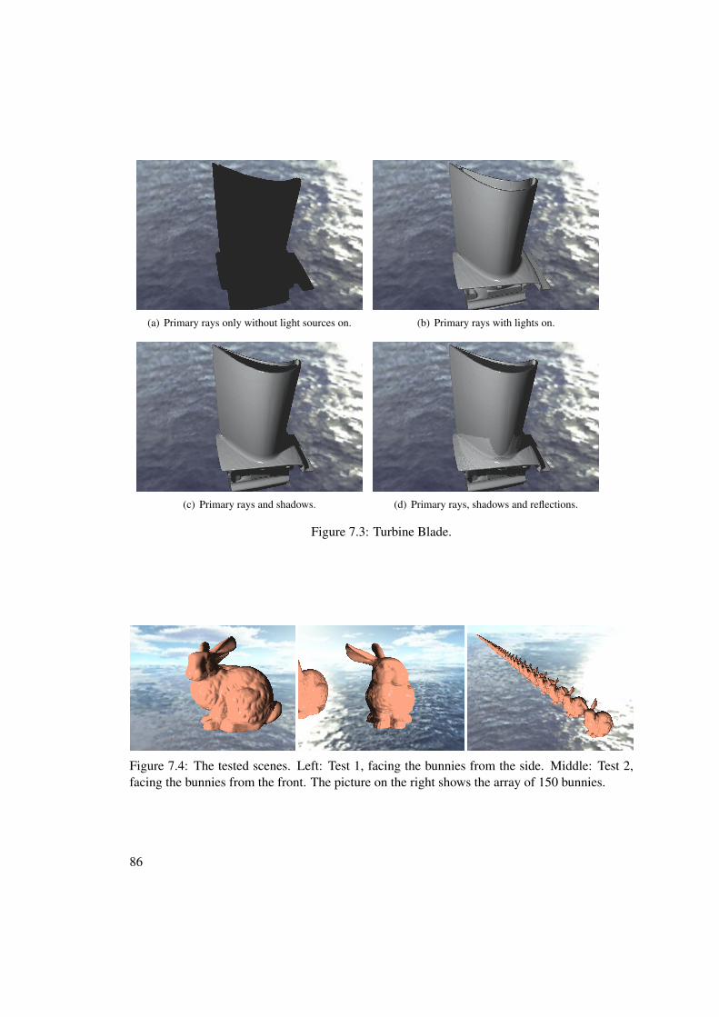
(a) Primary rays only without light sources on. (b) Primary rays with lights on.

(c) Primary rays and shadows. (d) Primary rays, shadows and reflections.

Figure 7.3: Turbine Blade.

Figure 7.4: The tested scenes. Left: Test 1, facing the bunnies from the side. Middle: Test 2,facing the bunnies from the front. The picture on the right shows the array of 150 bunnies.

86

#BunniesScene 1 Scene 2

Object-kD-Trees Über-kD-Tree Object-kD-Trees Über-kD-Tree1 10 7 12 92 8 6 7 53 8 6 7 54 7 5 7 55 7 5 7 510 6 5 6.5 515 6 5 6 520 6 5 6 525 5.5 5 6 530 5 5 6 535 5 5 5 540 5 5 5 550 5 5 5 560 4 5 5 570 4 5 4 580 4 5 4 590 4 5 4 5100 4 5 4 5110 3 5 4 5120 3 5 3 5130 3 5 3 5140 3 5 3 5150 3 5 3 5

Table 7.6: This table shows the measured performances, given in FPS, for the two test scenes(see Figure 7.4). It can be seen that the performance of the Über-kD-Tree stays almost constant,whereas the performance of the Objects-kD-Trees decreases slowly with more and more objectsin the scene. The crossing point where the Über-kD-Tree has better performance for the givenscenes is around 60 objects.

therefore special code paths, some of the errors appeared only seldom. Since Nsight didnot work, there was no way to set breakpoints inside the CUDA code, nor was thereany other way to debug like one would do on the CPU. The solution was to rewrite thecomplete CUDA code in C# and introduce a “debug-pixel”. The debugging procedurewith the help of the debug-pixel is described in Section 6.6.

Despite all the troubles with debugging, however, the ray tracer is well debugged andworks without problems known so far.

• Data exchange between CUDA and C# and Aardvark integration

The first part of the thesis was the development of the CUDA library for Aardvark. Thislibrary needed to provide a way to maintain a mapping between dynamic C#-objects andCUDA-memory locations within hierarchical data structures and to provide the possibilityto update only certain parts (fields) within such data structures. Most of the data types used

87

in CUDA are organized in structs and arrays. In C#, structs are value types, which leadsto special maintenance for the mapping and support for data updates. To successfullyaccomplish and maintain such a mapping, several attempts have been implemented untila clean solution has been found.

Another time-consuming task was to implement graphics resource sharing between graph-ics APIs, like DirectX in versions 9 and 10, and CUDA. In Aardvark, the renderer is ab-stracted away behind a renderer interface. The problem was, however, that in the firstplace this interface did not allow access to certain low-level data like the DirectX resourcepointers, which are needed to implement graphics resource sharing with CUDA.

• HILITE interface

Concurrently to the development of the ray tracer, the HILITE-Viewer, which is the mainrendering application of the HILITE project, was developed. One of the goals of theproject is a hybrid rendering algorithm, combining rasterization and ray tracing. To makethe integration of the ray tracer into the HILITE-Viewer as easy as possible, an additionallayer of abstraction between the CUDA-representation and the Aardvark-representationof the scene data had to be introduced. Furthermore, an interface had to be defined for thedata transition from the HILITE-Viewer into the CUDA ray tracer. Due to the ongoingdevelopment of the HILITE-Viewer, however, the requirements to this interface changedover time and several refactoring processes were necessary.

88

CHAPTER 8Conclusion and Future Work

8.1 Conclusion

In this thesis, I presented a CUDA ray tracer for the HILITE research-project at the VRVisresearch center. With the CUDA ray tracer it is possible to render correct curved reflectionswith interactive to real-time frame rates, depending on the scene complexity. The ray tracerruns completely on the GPU. Per pixel, one ray is traced in parallel using CUDA. The parallelray traversal was implemented in an iterative manner. From the geometry side, the ray tracercan handle triangle meshes. Multiple reflection bounces and shadows for directional and pointlight sources are supported and can be fully configured interactively at runtime. The ray tracerwas integrated by another student into the HILITE Viewer, the main application of the HILITE-project, during the writing of the thesis.

As far as acceleration structures are concerned, the ray tracer supports two variants of kD-Trees (Section 6.4). The first one is the Object-kD-Tree, which is a kD-Tree per geometricalobject in the scene. Since each object has its own transformation matrix, rigid animations arepossible with this data structure. The second variant is our newly developed Über-kD-Tree. TheÜber-kD-Tree is a two-level kD-Tree, having the Object-kD-Tree as leaves inside the Über-kD-Tree. Both kD-Tree variants are constructed on the CPU first, then converted to a GPU-capableformat and traversed on the GPU. The traversals of the kD-Trees are implemented as stack-basediterative traversals.

During research for available literature and resources, it turned out that it is hard to findcomplete algorithms on how to implement an iterative, massively parallel ray tracer in CUDA.The same holds true on how to store a kD-Tree in a GPU-capable format and how to implement astack-based iterative traversal for kD-Trees in CUDA. For these reasons, Chapter 4 summarizesthe algorithms for iterative and parallel ray tracing and diverse kD-Tree traversal methods.

It turned out that developing a complete ray tracer on the GPU, consisting of a few-thousandlines of code in a big CUDA kernel, is cumbersome to develop and to debug. What’s moreis that, since C# was the host language, most of the few debugging possibilities available forCUDA could not be used. To remedy this, the only solution was to rewrite the CUDA code in

89

C# and debug the code on the CPU. After debugging the CPU mirror-code, it was necessary totranslate the code back to CUDA. This slowed down development tremendously. Doing so, Icame up with a new method on how to debug the kD-Trees (Section 6.6). This can be appliedto all interactive CUDA rendering applications using acceleration data structures. KD-Trees arehard to debug in general, but because of the limited debugging possibilities on the GPU theyare even harder to debug there. The introduced debugging method uses a “debug pixel”. This isa fixed pixel on the screen for which CPU debugging can be triggered. This only works if theCPU representation of the kD-Tree code is an exact mirror of the GPU code. Otherwise, wrongcode paths will be debugged.

Finally, as a prerequisite to implement the ray tracer, a CUDA library for the VRVis-internalrendering engine has been developed. This has the advantage that research projects using Aard-vark can now utilize the power of GPU computing. The library has an easy-to-use interfacefor high-level access to CUDA functionality. CUDA resources like the CUDA-context, -device,-modules and -functions are managed by the library. It also provides memory management forGPU resources by a memory manager using a reference-counting scheme. A special challengewas that structs in C# are value types and can not be referenced by default. Hence, memorymanagement would not be possible with this data type. However, besides arrays, they are themost important ones for GPU computing. The most satisfying solution to this was finally toencapsulate the structs into an array of length 1. When working with CUDA, the data types usedmost of the time are either arrays or compound types like structs. For this reason, ready-to-usedata types have been created, which can be used from within C# as normal C#-objects, as well asfrom CUDA. Whats more is that CUDA-kernels can be called almost like any other C#-function,providing flexibility and convenience when working with CUDA. This way, one does not haveto worry about parameter mappings and conversion issues. To provide efficient data sharing be-tween CUDA and graphics APIs, graphics resource sharing has been implemented as well, evenif Aardvark did not support the needed low-level access to graphics resources in the first place.Finally, the library also supports CUDA-Streams and -Events for parallel kernel execution andtiming measurements.

8.2 Future Work

Even if the targeted goals of this diploma thesis have been met, there are lots of possibilities toenhance and extend the ray tracer.

The first one is the integration into the HILITE Viewer, the main application of the HILITEproject. During writing of this thesis, this task has already been done by another student.

In order to achieve better photorealism, transparency should be implemented. Further, com-mon effects like depth of field, motion blur, ambient occlusion, subsurface scattering and softshadows are also candidates for future implementations.

Another important feature would be the implementation of multi-sampling and anti-aliasing,as well as adaptive rendering in such a way, that when the camera moves and the frame rate dropstoo low, only each n-th pixel is rendered. To enhance rendering time, algorithms like packettraversal (as described in Section 2.3.2) could be added as well. Additionally, hybrid rendering

90

could be implemented by handling the primary rays with rasterization and then starting the raytracing task for the secondary rays only.

Furthermore, the CUDA code could be even further optimized. Especially the time formemory access can be reduced. To avoid the penalty of threads in a warp waiting for longerrunning threads in this warp to finish, ray pools and persistent threads as in [AL09] could beimplemented as well.

Since the construction of the kD-Trees on the CPU take a considerable amount of timeespecially for bigger scenes, it would be nice to implement kD-Tree construction on the GPU.

An interesting research topic would be the implementation of BVHs and to compare theirperformance to kD-Trees in terms of rendering performance, construction time and memoryfootprint.

Besides that, the CUDA library currently supports the CUDA 3.x API and parts of the 4.xAPI, which are incompatible with the newer versions of Nvidia’s debugging-tool Nsight. Hence,the API should be updated to fully support version 4.x.

91

Bibliography

[AK87] James Arvo and David Kirk. Fast Ray Tracing by Ray Classification. InProceedings of the 14th annual conference on Computer graphics and interactivetechniques, SIGGRAPH ’87, pages 55–64, New York, NY, USA, 1987. ACM.

[AK11] C. Wächter A. Keller. Efficient Ray Tracing without Auxiliary Acceleration DataStructures, 2011. HPG 2012, Poster.

[AL09] Timo Aila and Samuli Laine. Understanding the Efficiency of Ray Traversal onGPUs. In Proceedings of the Conference on High Performance Graphics 2009,HPG ’09, pages 145–149, New York, NY, USA, 2009. ACM.

[ALK12] Timo Aila, Samuli Laine, and Tero Karras. Understanding the Efficiency of RayTraversal on GPUs - Kepler and Fermi Addendum. NVIDIA Technical ReportNVR-2012-02, NVIDIA Corporation, June 2012.

[Ben75] Jon Louis Bentley. Multidimensional Binary Search Trees used for AssociativeSearching. Commun. ACM, 18(9):509–517, September 1975.

[Bik11] Jacco Bikker. Arauna - Real-time Ray Tracing. http://igad.nhtv.nl/~bikker, 2011. Last accessed: 23nd of February, 2013.

[Cab10] João Cabeleira. Combining Rasterization and Ray Tracing Techniques to Approx-imate Global Illumination in Real-Time. Master’s thesis, Technical University ofLisbon, Instituto Superior Técnico, 2010.

[CG] Inc. Caustic Graphics. CausticOne. https://caustic.com/caustic-rt_caustic-one.php. Last accessed: 22nd of April, 2013.

[Cooa] Nvidia Coorp. CUDA. http://developer.nvidia.com/category/zone/cuda-zone. Last accessed: 23nd of February, 2013.

[Coob] Nvidia Coorp. CUDA LLVM Compiler. https://developer.nvidia.com/cuda-llvm-compiler. Last accessed: 16nd of April, 2013.

[Cooc] Nvidia Coorp. CUDA Programming Guide, Version 4.2. Part of the CUDA SDK.Downloadable at http://developer.nvidia.com. Last accessed: 23nd ofFebruary, 2013.

93

[Coo10] Nvidia Coorp. NVIDIA’s Next Generation CUDA Compute Architecture: Fermi,2010. Whitepaper.

[DPS10] P. Danilewski, S. Popov, and P. Slusallek. Binned SAH kD-Tree Construction on aGPU. Technical report, Saarland University, 2010.

[EMD+05] Pau Estalella, Ignacio Martin, George Drettakis, Dani Tost, Olivier Devillers, andFrederic Cazals. Accurate Interactive Specular Reflections on Curved Objects. InIn Proc. of VMV 2005, 2005.

[EMDT06] Pau Estalella, Ignacio Martin, George Drettakis, and Dani Tost. A GPU-drivenAlgorithm for Accurate Interactive Reflections on Curved Objects. In Proceedingsof the 17th Eurographics conference on Rendering Techniques, EGSR’06, pages313–318, Aire-la-Ville, Switzerland, Switzerland, 2006. Eurographics Association.

[Áfr12] Attila T. Áfra. Incoherent Ray Tracing without Acceleration Structures. Euro-graphics 2012 short paper, 2012.

[FS05] Tim Foley and Jeremy Sugerman. KD-Tree Acceleration Structures for a GPURaytracer. In Proceedings of the ACM SIGGRAPH/EUROGRAPHICS conferenceon Graphics hardware, HWWS ’05, pages 15–22, New York, NY, USA, 2005.ACM.

[GAS] Company for Advanced Supercomputing Solutions Ltd. GASS. CUDA.NET.http://www.cass-hpc.com/category/cudanet. Last accessed: 23nd

of February, 2013.

[GL10] Kirill Garanzha and Charles T. Loop. Fast Ray Sorting and Breadth-First PacketTraversal for GPU Ray Tracing. Comput. Graph. Forum, 29(2):289–298, 2010.

[Gmb] VRVis GmbH. HILITE. http://vrvis.at/projects/hilite. Last ac-cessed: 23nd of February, 2013.

[GPM11] Kirill Garanzha, Jacopo Pantaleoni, and David McAllister. Simpler and fasterHLBVH with Work Queues. In Proceedings of the ACM SIGGRAPH Symposiumon High Performance Graphics, HPG ’11, pages 59–64, New York, NY, USA,2011. ACM.

[GPP+10] Olivier Gourmel, Anthony Pajot, Mathias Paulin, Loïc Barthe, and Pierre Poulin.Fitted BVH for Fast Ray Tracing of Metaballs. Computer Graphics Forum, 29(2),May 2010.

[GS87] Jeffrey Goldsmith and John Salmon. Automatic Creation of Object Hierarchies forRay Tracing. IEEE Comput. Graph. Appl., 7(5):14–20, May 1987.

[Gue08] Paul Guerrero. Approximative Real-time Soft Shadows and Diffuse Reflectionsin Dynamic Scenes. Master’s thesis, Vienna Unitersity of Technology, Institute ofComputer Graphics and Algorithms, 2008.

94

[Hav00] Vlastimil Havran. Heuristic Ray Shooting Algorithms. PhD thesis, Faculty ofElectrical Engineering, Czech Technical University, Prague, 2000.

[HBZ98] Vlastimil Havran, Jirí Bittner, and Jirí Zára. Ray Tracing with Rope Trees. Inin Proceedings of 13th Spring Conference On Computer Graphics, Budmerice inSlovakia, pages 130–139, 1998.

[Hec90] Paul S. Heckbert. Adaptive Radiosity Textures for Bidirectional Ray Tracing. InProceedings of the 17th annual conference on Computer graphics and interactivetechniques, SIGGRAPH ’90, pages 145–154, New York, NY, USA, 1990. ACM.

[HQL+10] Qiming Hou, Hao Qin, Wenyao Li, Baining Guo, and Kun Zhou. MicropolygonRay Tracing with Defocus and Motion Blur. In ACM SIGGRAPH 2010 papers,SIGGRAPH ’10, pages 64:1–64:10, New York, NY, USA, 2010. ACM.

[HSHH07] Daniel Reiter Horn, Jeremy Sugerman, Mike Houston, and Pat Hanrahan. In-teractive kD-Tree GPU Raytracing. In Proceedings of the 2007 symposium onInteractive 3D graphics and games, I3D ’07, pages 167–174, New York, NY, USA,2007. ACM.

[ICG86] David S. Immel, Michael F. Cohen, and Donald P. Greenberg. A Radiosity Methodfor Non-Diffuse Environments. In Proceedings of the 13th annual conference onComputer graphics and interactive techniques, SIGGRAPH ’86, pages 133–142,New York, NY, USA, 1986. ACM.

[Kaj86] James T. Kajiya. The Rendering Equation. In Proceedings of the 13th annualconference on Computer graphics and interactive techniques, SIGGRAPH ’86,pages 143–150, New York, NY, USA, 1986. ACM.

[KBS11a] Javor Kalojanov, Markus Billeter, and Philipp Slusallek. Two-Level Grids for RayTracing on GPUs. In Oliver Deussen Min Chen, editor, EG 2011 - Full Papers,pages 307–314, Llandudno, UK, 2011. Eurographics Association.

[KBS11b] Javor Kalojanov, Markus Billeter, and Philipp Slusallek. Two-Level Grids for RayTracing on GPUs. Computer Graphics Forum, 30(2):307–314, 2011.

[KK86] Timothy L. Kay and James T. Kajiya. Ray Tracing Complex Scenes. InProceedings of the 13th annual conference on Computer graphics and interactivetechniques, SIGGRAPH ’86, pages 269–278, New York, NY, USA, 1986. ACM.

[Lás99] Szirmay-Kalos László. Monte-Carlo Methods in Global Illumination, 1999. Scrip-tum.

[MB05] Marc Stamminger Marcel Beister, Manfred Ernst. A hybrid gpu-cpu renderer.Vision, Modeling, and Visualization 2005, 2005.

[MM95] Michael John Muuss and Michael John Muuss. Towards Real-Time Ray-Tracingof Combinatorial Solid Geometric Models, 1995.

95

[Mor66] G. M. Morton. A Computer Oriented Geodetic Data Base; and a new Technique inFile Sequencing. Technical report, IBM Ltd., Ottawa, Canada, 1966.

[Mor11a] Benjamin Mora. Direct-Trace Library: Ray Tracing for the Masses. http://www.directtrace.org, 2011. Last accessed: 23nd of February, 2013.

[Mor11b] Benjamin Mora. Naive Ray Tracing: A Divide-and-Conquer Approach. ACMTrans. Graph., 30(5):117:1–117:12, October 2011.

[M.R85] Kaplan M.R. Space Tracing: A Constant Time Ray Tracer, State of the Art inImage Synthesis. In SIGGRAPH ’85 course notes, page 11f, 1985.

[PBD+10] Steven G. Parker, James Bigler, Andreas Dietrich, Heiko Friedrich, Jared Hobe-rock, David Luebke, David McAllister, Morgan McGuire, Keith Morley, AustinRobison, and Martin Stich. OptiX: A General Purpose Ray Tracing Engine. InACM SIGGRAPH 2010 papers, SIGGRAPH ’10, pages 66:1–66:13, New York,NY, USA, 2010. ACM.

[PBMH02] Timothy J. Purcell, Ian Buck, William R. Mark, and Pat Hanrahan. Ray Tracing onprogrammable Graphics Hardware. In Proceedings of the 29th annual conferenceon Computer graphics and interactive techniques, SIGGRAPH ’02, pages 703–712,New York, NY, USA, 2002. ACM.

[PGDS09] Stefan Popov, Iliyan Georgiev, Rossen Dimov, and Philipp Slusallek. Object Par-titioning considered harmful: Space Subdivision for BVHs. In Proceedings of theConference on High Performance Graphics 2009, HPG ’09, pages 15–22, NewYork, NY, USA, 2009. ACM.

[PGSS06] S. Popov, J. Günther, Hans-Peter Seidl, and P. Slusallek. Experiences with Stream-ing Construction of SAH kD-Trees. IEEE Symposium on Interactive Ray Tracing,pages 89–94, 2006.

[PL10] J. Pantaleoni and D. Luebke. HLBVH: Hierarchical LBVH Construction for Real-time Ray Tracing of Dynamic Geometry. In Proceedings of the Conference onHigh Performance Graphics, HPG ’10, pages 87–95, Aire-la-Ville, Switzerland,Switzerland, 2010. Eurographics Association.

[PMS+99] Steven Parker, William Martin, Peter-Pike J. Sloan, Peter Shirley, Brian Smits, andCharles Hansen. Interactive Ray Tracing. In Proceedings of the 1999 symposiumon Interactive 3D graphics, I3D ’99, pages 119–126, New York, NY, USA, 1999.ACM.

[RH06] David Roger and Nicolas Holzschuch. Accurate Specular Reflections in Real-Time. Computer Graphics Forum (Proceedings of Eurographics 2006), 25(3), sep2006.

96

[SFD09] Martin Stich, Heiko Friedrich, and Andreas Dietrich. Spatial Splits in Bound-ing Volume Hierarchies. In Proceedings of the Conference on High PerformanceGraphics 2009, HPG ’09, pages 7–13, New York, NY, USA, 2009. ACM.

[SPS07] Hans-Peter Seidel Stefan Popov, Johannes Günther and Philipp Slusallek. Stack-less kD-Tree Traversal for High Performance GPU Ray Tracing. Technical report,Saarland University, 2007.

[SSK07] Maxim Shevtsov, Alexei Soupikov, and Er Kapustin. Highly Parallel fastkD-Tree Construction for Interactive Ray Tracing of Dynamic Scenes. InEUROGRAPHICS 2007, volume 26, Number 3, 2007.

[Suf07] Kevin Suffern. Ray Tracing from the Ground Up. A K Peters/CRC Press, West-minster College, Salt Lake City, Utah, USA, 2007.

[SWW+04] Jörg Schmittler, Sven Woop, Daniel Wagner, Wolfgang J. Paul, and PhilippSlusallek. Realtime Ray Tracing of Dynamic Scenes on an FPGA Chip. InProceedings of the ACM SIGGRAPH/EUROGRAPHICS conference on Graphicshardware, HWWS ’04, pages 95–106, New York, NY, USA, 2004. ACM.

[Tra06] Gilles Tran. Glasses. Persistence of Vision Raytracer (POV Ray) - Hall of Fame,http://hof.povray.org, 2006. Last accessed: 23nd of February, 2013.

[WH06] Ingo Wald and Vlastimil Havran. On building fast kD-Trees for Ray Tracing,and on doing that in O(N log N). In IN PROCEEDINGS OF THE 2006 IEEESYMPOSIUM ON INTERACTIVE RAY TRACING, pages 61–70, 2006.

[Whi80] Turner Whitted. An improved Illumination Model for Shaded Display. Commun.ACM, 23(6):343–349, June 1980.

[WK06] Carsten Wächter and Alexander Keller. Instant Ray Tracing: The Bounding Inter-val Hierarchy. In IN RENDERING TECHNIQUES 2006 – PROCEEDINGS OFTHE 17TH EUROGRAPHICS SYMPOSIUM ON RENDERING, pages 139–149,2006.

[WMS06] Sven Woop, Gerd Marmitt, and Philipp Slusallek. B-KD Trees for HardwareAccelerated Ray Tracing of Dynamic Scenes. In Proceedings of the 21st ACMSIGGRAPH/EUROGRAPHICS symposium on Graphics hardware, GH ’06, pages67–77, New York, NY, USA, 2006. ACM.

[WS05] Sven Woop and Jörg Schmittler. RPU: A Programmable Ray Processing Unit forRealtime Ray Tracing. In ACM Trans. Graph, pages 434–444, 2005.

[WSB01] Ingo Wald, Philipp Slusallek, and Carsten Benthin. Interactive Distributed RayTracing of Highly Complex Models. In In Rendering Techniques 2001: 12thEurographics Workshop on Rendering, pages 277–288. Springer, 2001.

97

[WSBW01] Ingo Wald, Philipp Slusallek, Carsten Benthin, and Markus Wagner. InteractiveRendering with Coherent Ray Tracing. In Computer Graphics Forum, pages 153–164, 2001.

[WZL11] Zhefeng Wu, Fukai Zhao, and Xinguo Liu. SAH KD-Tree Construction on GPU. InProceedings of the ACM SIGGRAPH Symposium on High Performance Graphics,HPG ’11, pages 71–78, New York, NY, USA, 2011. ACM.

[ZHWG08] Kun Zhou, Qiming Hou, Rui Wang, and Baining Guo. Real-time kD-Tree Con-struction on Graphics Hardware. In ACM SIGGRAPH Asia 2008 papers, SIG-GRAPH Asia ’08, pages 126:1–126:11, New York, NY, USA, 2008. ACM.

98