Dominance Relationship Analysis with Budget Constraints

Shen Ge #1 Leong Hou U ∗2 Nikos Mamoulis #3 David W.L. Cheung #4

#Department of Computer Science, University of Hong Kong

Pokfulam Road, Hong Kong1sge@cs.hku.hk 3nikos@cs.hku.hk 4dcheung@cs.hku.hk

∗Department of Computer and Information Science, University of Macau

Av. Padre Tomas Pereira Taipa, Macau2ryanlhu@umac.mo

Abstract

Customers typically buy products after comparing their features, thus several market analysis tasks(e.g., skyline computation) perform dominance analysis between products. In this paper, we study aninteresting problem in this class, which has not received enough attention by past research. An importantdecision problem by a company is how to design a new product, which dominates all its competitors.Designing the perfect product, however, might not be feasible since in practice the development pro-cess is confined by some constraints, e.g., limited funding or low target selling price. We model theseconstraints by a constraint function which determines the feasible characteristics of a new product. Giv-en such a budget, our task is to decide the best possible features of the new product that maximize itsprofitability. In general, a product is marketable if it dominates a large set of existing products, whileit is not dominated by many. Based on this, we define dominance relationship analysis (DRA) and useit to measure the profitability of the new product. The decision problem is then modeled as a budgetconstrained optimization query (BOQ). Computing BOQ is challenging due to the exponential increaseof the search space with dimensionality. We propose a divide-and-conquer based framework which out-performs a baseline approach in terms of not only execution time but also space complexity. Based onthe proposed framework, we further study an approximation solution which provides a good tradeoffbetween computation cost and quality of result.

1 IntroductionRecently, there has been a lot of interest in the database and data mining communities on market analysisproblems, related to product profitability and promotion [11, 21, 13, 17, 19, 24, 18]. Most of these worksmodel products as points in the high dimensional space defined by a set of features; the dominance rela-tionships between these points are then used to infer the relative influence of the corresponding products inthe market. In this paper, we study an important problem in this class, which has not been considered bypast research.

Given a set of existing products O in the market and a development budget B, our task is to decide thebest possible features of a new product that maximize its profitability and fit the budget B. For example,consider the development of a new laptop computer by a manufacturer. Typically, performance and mobilityare two primary features that customers care when choosing a laptop. Assuming that the selling price isconstrained, the manufacturer may find it hard to create a new laptop that maximizes the quality of bothfeatures at the same time. A feasible solution may either have to sacrifice performance (e.g., using a low-end processor) or to reduce mobility (e.g., replacing a 6-cells by a 4-cells battery), in order to fit the targetprice.

Web advertising is another example. A provider wants to create a new advertisement package thatfits the typical service price and also make the package attractive to the potential customers. A customermay consider the following features for her ad: the position of the ad in the web page and the length of

1

display time. An ad is more expensive if it is displayed at a good position for a long time. Assuming thatthe service provider has a targeted service price, our task is to create a new package that dominates mostexisting products in the market. Once again, the problem is to find the optimal feature values, constrainedby a budget (the service price).

Motivated by these examples, in this paper, we study a new query, called budget constrained optimiza-tion query (BOQ). Typically, manufacturers do not have infinite development funding and must considerdifferent trade-offs and constraints when they do research and development for their products. Given a setof products O in the market and a budget B, the goal of BOQ is to identify the features of a new productx such that x fits the budget B and its profitability is maximized. This new data analysis query is formallydefined as Problem 1 below:

Problem 1 (Budget Constrained Optimization). Given a budget B, a constraint function C(x), and anobjective function f(x), create a new product x such that C(x) ≤ B and the objective function f(x) ismaximized.

Constraint function C(x). We consider constraint functions C(x), which monotonically change with thevalues of the features (i.e., dimensions) of x. This implies that for C(x) to remain constant, if a featurevalue increases, there should be another feature of decreasing value. The weights of different features inthe function could differ and the function is not necessarily a linear combination of the features. In thiswork, C(x) is modeled by a set of monotone functions, which are highly flexible and widely used in manyworks.

C(x) is a generalized concept and is defined by domain experts in general. For instance, the value ofan NBA player can be calculated by the approximate value function (AV function) given in [14]. The AVfunction is monotonic to the players’ performance, increasing with all positive factors (points, rebounds,etc.) and decreasing with all negative factors (field goals missed, turnovers, etc.). The AV function is anexample of a constraint function in a real application that measures the value of objects based on theircapabilities.

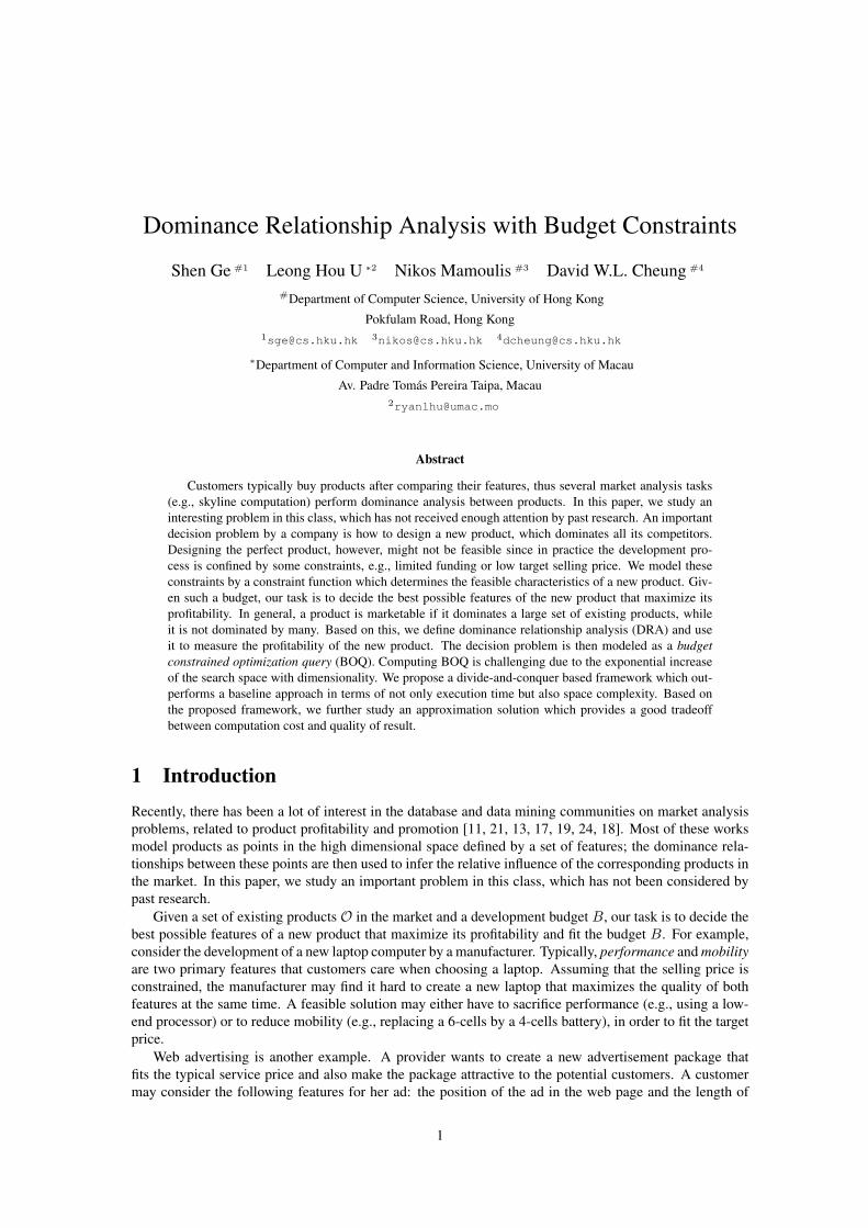
We use NBA players statistics to demonstrate the relationship between players capacities (profitability)and salaries (cost). We plot the average points and assists of guard players in 2007-2008, in data collectedfrom [1]. These two are the main features that characterize the capabilities of a guard. We also use salariesinformation from [2], to illustrate the top 100 paid guard players in Figure 1. Each player is displayed asa point on the points-assists plane, while different colors and markers are used to distinguish players withdifferent salary scales.

2

4

6

8

10

12

assi

sts

per g

amep

lay

Top 1-20 Top 21-40 Top 41-60 Top 61-80

0

2

4

6

8

10

12

0 5 10 15 20 25 30 35

assi

sts

per g

amep

lay

points per gameplay

Top 1-20 Top 21-40 Top 41-60 Top 61-80

Figure 1: Average points and assists performance of the top paid guard players in NBA

The figure shows the general trend that, the higher the salary, the better the capabilities. This coincideswith our intuition that if our budget is large, our space of choice becomes larger, and thus we can find betterplayers. Also notice that, for the same salary level, there are tradeoffs between the two capability values,which prevent us from maximizing both two values at the same time under a budget constraint.

Objective function f(x). f(x) is the second and equally important component of BOQ, used to measure

2

the quality of a product based on the concept of dominance, as shown in Definition 1.

Definition 1 (Dominance). A product x is definitely better than (dominates, ≺) another product x′ if andonly if every feature of x is not worse than the corresponding feature of x′ and there is at least one featurewhere x is strictly better.

In general, a product is marketable if it dominates a large set of existing products and it is not dominatedby many. [11] was the first work to propose a definition for profitability based on dominance, which weextend here to define the objective function f(x):

f(x) = (1 + β)dc+(x)− (1− β)dc−(x) (1)

In Eq. 1, dc+(x) is the number of objects being dominated by x, dc−(x) is the number of objects dominat-ing x, and β is a parameter adjusting the relative weights between dc+(x) and dc−(x), which is set to 0 bydefault, giving an equal weighting to both sides. A large value of f(x) implies a product x, which is betterthan a large set of competitors while being worse to only few of them. If there was no budget constraint, wecould develop a product with the best possible values in all features, which would dominate all products inthe market, while being dominated by none of them; thus, the optimization problem is meaningless withoutthe constraint C(x) ≤ B.

In the rest of the paper, we make the convention that smaller feature values are better. To be consistentwith this assumption, we also assume that the constraint function is antimonotonic to the feature values;that is, if x[i] ≤ y[i] in every dimension i, then C(x) ≥ C(y). Figure 2 demonstrates BOQ. Given a setof laptop computers O with two features (performance and mobility), a constraint function C(x), and adevelopment budgetB, as shown in the figure, our task is to determine the best possible features of the newproduct x such that C(x) ≤ B and f(x) = dc+(x) − dc−(x) is maximized (assuming smaller values ineach dimension are better). Given three candidates x1, x2, and x3, their profitabilities calculated by f(x)are 3, 2, and 2 respectively; thus, x1 is the best over these candidates. In Figure 2(b), we show 11 feasibleprofitable regions, shaded in gray, on top of the budget plane C(x) = B. These regions are defined bythe points on the line C(x) = B, where the line intersects the hyperplanes orthogonal to existing products(indicated by black dots). After the partitioning, all points within each region have identical profitabilities,while satisfying the objective function. For each region, we can easily measure the profitability by countingthe products it dominates / it is dominated by. For example, the region with the highest profitability is r9;∀x ∈ r9, f(x) = 3 (e.g., f(x1) = 3).

mobility

pe

rfo

rma

nce

x1

x2

C(x)=B

x3

o1

o2

o3

o4

o5

o6

(a) Computation of BOQ

mobility

pe

rfo

rma

nce r1

r2 r3

r4 r5

r6 r7

r8 r9r10

r11

x1

o1

(b) Profitable Regions

Figure 2: Examples of BOQ

In general, it is more desirable to identify the most profitable regions (as in Figure 2(b)), instead ofsimply comparing some random candidate products (as in Figure 2(a)). First, this offers flexibility to thedeveloper to choose from a range of possible feature value combinations that fall in the most profitable

3

regions. Second, she might minimize the production cost (while maximizing the profit) by choosing thepoint x in the most profitable regions, which has the lowest C(x) value (i.e., the upper right corner of r9

in our example). Therefore, we define a generalization of BOQ (GenBOQ), which returns a set of regionsthat share the best profitability instead of a single object in BOQ.

Problem 2 (General BOQ). Given a budget B, a constraint function C(x), and an objective functionf(x), a general BOQ returns a set of regions R such that C(x) ≤ B and the objective function f(x) ismaximized, ∀x ∈ R.

The big challenge of the query is the huge solution search space. Instead of verifying infinite potentialproducts on the continuous budget plane, a possible (baseline) approach is to generate compact regions bydrawing orthogonal hyperplanes from each existing object (as shown in Figure 2(b)). However, as we showin the following lemma, the number of compact regions is O(d ·nd−1), in a d-dimensional problem with nexisting products.

Lemma 1 (Number of compact regions). The number of compact regions that can be generated in a d-dimensional problem with n objects is O(d · nd−1).

Proof. Suppose there are n discrete objects in d dimensional space, the entire space can be split by thesen objects into O(nd) regions (i.e., Minimum Bounding Rectangles, MBRs). The problem is now to findhow many these O(nd) regions intersect the budget plane BP , in the worst case. The largest BP can beconstructed by d orthogonal hyperplanes, each of which is orthogonal to one axis i and its i-th featurevalue is set to the minimum value. The intersection point of all hyperplanes is the minimum corner in theentire space. Therefore, each hyperplane intersects O(nd−1) regions and we have d hyperplanes; the totalnumber of compact regions is O(d · nd−1).

To address this space growth challenge, we develop an efficient divide-and-conquer framework thatpartitions the space recursively. Our approach greatly outperforms the baseline method in terms of responsetime. In addition, we reduce the memory requirements from O(d ·nd−1) to O(θd−1), where θ is a constantthat expresses a tradeoff between computational cost and space. Our contributions can be summarized asfollows:

• We study a new market analysis problem that can help manufacturers to design a new product with-in a development budget such that the profitability is maximized. This problem can be solved byour proposed budget constrained optimization query (GenBOQ). We believe that GenBOQ can bea valuable decision making tool for manufacturers; furthermore, it can be used by data analysts toexamine the product space.

• We show that a naıve solution to GenBOQ is infeasible due to its high execution time and extremespace consumption. We propose a Divide-and-Conquer (D&C) paradigm paired with some opti-mization techniques which renders GenBOQ evaluation on large problems feasible. We provide atheoretical analyses for the costs of all discussed algorithms.

• To further reduce the response time, we propose an approximation algorithm for GenBOQ queriesthat can return approximate results with a quality control parameter.

• We demonstrate the scalability of all proposed methods using synthetic and real data. Our experi-mental result is consistent to our theoretical analysis. Furthermore, we experimentally show that anadaptation of a previous approach [11] to solve our problem is not only inaccurate but also inefficient.

The rest of the paper is organized as follows. Section 2 presents related work. Preliminary concepts andproperties are introduced in Section 3. In Sections 4 and 5 we present our solution and Section 6 evaluatesit. The paper is concluded in Section 7. Table 1 summarizes the notation that will be used throughout thepaper.

4

Table 1: Summary of NotationSymbol Meaning

B the development budget

C(x) the constraint function

f(x) the objective function

BP budget plane which is defined by C(x) = B

O the set of objects

oi an object in OM the set of MBRs

T quality tolerance bound

2 Related Work

2.1 Dominance Relationship AnalysisOur problem is very close to the work on dominance relationship analysis (DRA) [11, 21, 20] and domina-tion game analysis [24].

Ref. [11] was the first paper for business analysis from a microeconomic perspective using the conceptof dominance. The authors proposed a data cube model (DADA), to summarize all the domination rela-tionships between objects in all dimensions, in a bottom-up fashion. In DADA, the space is divided intoDom1 ×Dom2 × . . .×Domd cells, where Domi is the number of discrete values stored in dimension i;the objects inside the same cell have identical domination relationships. Furthermore, the authors proposeda D*-tree to group all neighboring cells with the same domination count; this facilitates efficient search.It is shown that this data organization model can efficiently support three query types related to microe-conomic problems: Linear Optimization Query (LOQ), Subspace Analysis Query (SAQ) and ComparativeDominant Query (CDQ).

The definition of our GenBOQ is similar to LOQ proposed in [11]. However, our problem has two maindifferences: (i) Our GenBOQ supports any combination of monotone functions while LOQ merely modelsthe budget constraint as a single linear function. (ii) DADA can only return a set of cells that maximizethe objective function instead of compact regions as proposed in our work. We demonstrate difference (ii)using Figure 3(a). Suppose that there are three objects in the two dimensional space and DADA regularlydivides the space into 4 cells. The domination scores f(x) are shown at the left bottom corners of thecells. DADA will return cell 0 for LOQ since this cell has the maximum domination score among all fourcells. Nevertheless, the best feasible region in cell 0 (i.e, the shaded triangle r2 in the middle of the figure)is not the best region; its domination score is −1, which is worse than the scores of the best triangularregions in cells 1 and 2 (i.e., r1 and r3). DADA could return the correct result for LOQ only if the involveddimensions have discrete domains. However, the computational cost becomes prohibitive if the domain ofdiscrete values is large, as we demonstrate in Section 6.

Yang et al. in [20] and [21] study some extensions of DRA. In [21], a special data cube called ParCubethat supports dominance relationships analysis on partially ordered dimensions is proposed. They proposedalgorithms for updating their index structure and return the exact objects dominated rather than just theirtotal number (as in [11]). [20] relaxes the dominance relationship and compresses the index with suchdominance relationships encoded; in addition, it proposes some efficient strategies to support querying onrelaxed dominant relationships. However, all these methods are built on the data cube concept and none ofthem can compute the exact result of our problem.

Domination game analysis for microeconomic data mining is studied in [24]. Given a set of customersand a set of manufacturers, each manufacturer creates only one product to the market for fairness. The taskof the domination game is to find a configuration of the products that achieves stable expected market sharesfor all products. A product is said to dominate a customer if all its features can satisfy the requirementsof the customer. The expected market share of a product is measured by the expected number of buyers

5

mobility

pe

rfo

rma

nce cell 3

3

1

1

0

C(x)=BDADA feasible

region

best feasible

regions

cell 1

cell 0 cell 2

r1

r2

r3

(a) with DADA

mobility

pe

rfo

rma

nce

best feasible

region

skyline points

C(x)=B

r

(b) with skyline

Figure 3: Comparison of our query with other types of queries.

in the customers, all of which are equally likely to buy any product dominating them. A depth-first and abreadth-first search strategy are proposed along with a set of pruning techniques for the search space. Thetechniques proposed in [24] cannot be used for our problem, because they find a configuration rather thana set of regions that maximize an objective function.

2.2 SkylineThere is plenty of work on skyline evaluation (e.g., [5, 16, 9, 6, 15, 23]). The concept of skyline is basedon the dominance relationship and originated from the maximal vector computation problem [10].

The objective of skyline queries is to find the objects that are not dominated by others. Skyline querieswere first introduced in a database context in [5], where approaches using block nested loop (BNL) anddivide-and-conquer (D&C) were proposed. Since then, several efficient methods for skyline computationhave been proposed. These include the bitmap method [16], sorted first skyline (SFS) [6], nearest neighbor(NN) based skyline evaluation [9], and branch and bound skyline (BBS) [15]. BBS [15] is an incrementalskyline algorithm that accesses a minimal number of nodes from an R-tree [4] that indexes the data (i.e., anI/O optimal algorithm in this context). An object-based space partitioning method that provides efficientskyline computation in high dimensional spaces was proposed in [23]].

Several variants to the basic skyline query also exist. Reverse skyline search [12] aims at finding thepoints that have a given query point in their dynamic skyline [15, 8]. The top-k dominating query, studied in[22] returns k data objects that dominate the largest number of objects in the dataset. The main differencesbetween this method and our work are (i) this method searches in the much smaller search space of the dataobjects to find the best one and (ii) we consider both dominating and dominated objects. In fact, no skylinemethod can be adjusted to solve our problem. This is because our query finds compact regions insteadof existing objects, which span a much larger space (O(d · nd−1) regions vs. n, according to Lemma 1).In addition, the best compact regions are not guaranteed to be determined by skyline points only. Forexample, in Figure 3(b), the gray area denotes the best feasible region r. We can easily see that r cannotbe constructed even if we know all skyline points (i.e., the skyline operator cannot be used to solve theGenBOQ query).

2.3 Related QueriesMiah et al. [13] studied an optimization problem that selects a subset of attributes of a product t, such thatt’s shortened version still maximizes t’s visibility to potential customers. This problem is NP-hard; severalexact and approximate algorithms are proposed. This problem has a different definition compared to ourproblem, but shares the intuition that manufacturers want to cut down a development cost.

In [19], the authors studied a problem to find a subset of object o’s features so that o is ranked highly inthe found subspace. They call this promotion analysis through ranking; this is a challenging problem due

6

to the explosion of the search space and the high aggregation cost. They proposed a PromoRank frameworkand an efficient algorithm using subspace pruning, object pruning and promotion cube. Since the aim is tofind the promotive subspace for some specified objects, this framework cannot suggest possible positionsfor newly developed products. Also, it does not consider budget constraints.

Creating competitive products from a pool of possible dimensional values is studied in [17]. Theobjective is to find a set of newly created objects according to some generating rules, which cannot bedominated by any existing products in the market. Instead of generating and checking all possible newobjects, [17] uses group partitioning with partial pruning so that only a small subset of the new possibleobjects are considered. The idea of finding good possibilities for new product is basically the same withours. However, we can suggest regions for new products even without knowing how these new productscan be generated. Also, as opposed to [17], we consider budget constraints.

Recently, Wan et al. [18] proposed a problem that selects the top-k profitable products from a set ofnew products Pnew. For each product, all the features other than price are known. The problem is toassign appropriate prices to k products from Pnew such that these products are not dominated by otherexisting products in the market. This problem is shown to be NP-hard when there are 2 or more dimensionsin the feature space and can be approximately solved by greedy methods. We share the same intuitionas this work, which also creates new products that maximize an objective confined by constraints. Theirobjective is to create k new skyline products, while our objective is to find candidate products having thebest domination score. Their constraint is the set of possible new products, while our constraint is a valueof function C(x).

3 PreliminariesIn this section, we define concepts and present properties that are used in our solutions. We assume a datasetO of n data objects O = {o1, o2, . . . , on} in a d dimensional space. Each object oi = (oi[1], . . . , oi[d])models the feature vector of an existing product in the market. We assume that for each feature, smallervalues indicate better quality. Given a constraint function C and a development budget B, we define thebudget plane as follows.

Definition 2 (Budget plane). The budget plane BP is a d − 1 dimensional surface, on which all pointshave the same development budget B. Formally, BP is the area defined by C(x) = B.

The objects are classified into two categories, positive object setO+ and negative object setO−, basedon Definition 3. Broadly speaking, an object is in O+ if it can add to the profitability of the new product.For instance, O+ = {o1, o2, o3, o4} and O− = {o5, o6} in Figure 2(a).

Definition 3 (Positive/Negative object set). Set O+ (O−) denotes the objects in O for which C(o) < B(C(o) ≥ B).

After classifying the objects, we can define the set of objects that dominate or are dominated by agiven object o in Definition 4. In Section 1, we defined dc+(o) (dc−(o)) as the number of objects that aredominated by (dominate) o. We have dc+(o) = |D+(o)| and dc−(o) = |D−(o)|.

Definition 4 (Dominance set). D+(o) denotes the set of objects in O+ which are dominated by object o.Similarly, D−(o) denotes the set of objects in O− dominating o.

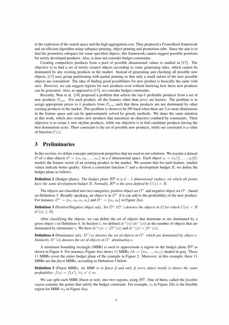
A minimum bounding rectangle (MBR) is used to approximate a region on the budget plane BP asshown in Figure 4. For instance, Figure 4(a) shows 11 MBRsM := {m1, ...,m11} shaded in gray. These11 MBRs cover the entire budget plane of the example in Figure 2. Moreover, in this example, these 11MBRs are the finest MBRs, according to Definition 5 below.

Definition 5 (Finest MBR). An MBR m is finest if and only if every object inside it shares the sameprofitability: f(x) = f(x′), ∀x, x′ ∈ m.

We can split each MBR (finest or not), into two regions, using BP . One of them, called the feasibleregion contains the points that satisfy the budget constraint. For example, r9 in Figure 2(b) is the feasibleregion for MBR m9 in Figure 4(a).

7

Definition 6 (Feasible MBR region). The feasible region of MBR m, denoted by R(m) consists of allpoints x in m for which C(x) ≤ B.

mb

ma

mobility

pe

rfo

rma

nce

m1m2m3

m4 m5

m6

m7 m8

m9 m10

m11

mc

o4

o1

o2

o3

o5

o6

mub

muc

mlb

mlc

(a) 2D MBRs (b) 3D MBRs

Figure 4: Example of MBRs

In general, we can find a set of MBRs which cover the entire budget plane, e.g., the lightgray MBRs{ma,mb,mc} in Figure 4(a). However, one or more MBRs may not be finest, which means that the pointsin them do not share the same profitability. For instance, the right-top corner ml

b of MBR mb, which isthe point in it with the largest coordinates in all dimensions, is the lowest profitable point in mb. Theleft-bottom corner mu

b is the highest profitable point. Thus, for an MBR m, we can simply bound theprofitability of any point in m by [f(ml), f(mu)], which is the bounds of area inside the MBR.

In order to get the tightest upper and lower bounds, we refine the profitability bound for a MBR bydisregarding boundary cases. We note that the lower-left cornermu

c of MBRmc dominates (i.e., determinesthe profitability) all objects on the projected orthogonal line/hyperplane from mu

c . However, we do notconsider the boundary cases (e.g., o1) in fu(mc) since o1 is not dominated by any objects inside mc.More specifically, when calculating the profitability bound for a given MBR m, we consider only strictlydominated objects in the upper bound, making the bound tighter. The strict dominance relationship isdefined in Definition 7.

Definition 7 (Strict dominance set). D∆+(o) denotes the set of objects in O+ that are strictly dominatedby object o. Object o strictly dominates o′ if and only if every feature of o is strictly better than thecorresponding feature of o′. Similarly, D∆−(o) denotes the set of objects in O− strictly dominating o.

A tight upper profitability bound fu(m) for MBRm is computed by ignoring points that are not strictlydominated by the upper bound corner mu. Similarly, a tight lower bound f l(m) is computed by count-ing those objects that strictly dominate ml. These bounds are derived from Eq. 1 (i.e., the definition ofprofitability).

fu(m) := (1 + β)dc∆+(mu)− (1− β)dc−(mu) (2)f l(m) := (1 + β)dc+(ml)− (1− β)dc∆−(ml) (3)

dc∆+(mu) (dc∆−(ml)) is the number of objects in D∆+(mu) (D∆−(ml) ). For instance, [f l(mc),fu(mc)] = [1, 2] is the tightest profitable bound of mc, and objects o2 and o4 are in D∆+(mu

c ). Finally,we can determine whether an MBR is finest, using the following property.

Property 1. MBR m is finest if and only if fu(m) = f l(m).

The number of finest MBRs that cover the entire budget plane BP is O(d · nd−1), for n d-dimensionalobjects, as we show in Lemma 1. Figure 4(b) shows a 3D example. The entire BP is covered by 7 finestMBRs even though there is only one object, shown as a black point, in the domain space. In summary,finding the set of finest MBRs covering the entire BP is a hard problem.

8

4 Evaluation of GenBOQ

In this section we provide a comprehensive study on the evaluation of GenBOQ. First, we discuss the MBRrefinement algorithm, which serves as a baseline approach for our problem. Then, we outline a divide-and-conquer approach paired with some optimization techniques. In addition, we describe two alternativeapproaches, including a best-first search method with limited applicability and a hybrid approach thatcombines divide-and-conquer with best-first search. Finally, we analyze the complexity of MBR refinementalgorithm and D&C framework.

4.1 MBR Refinement Algorithm

As discussed, every object inside the same finest MBR shares the same profitability. Assuming that wehave a budget plane BP and a set of finest MBRs, the result of GenBOQ is the feasible region of one ormore of these MBRs. For example in Figure 4(a), m9 is the finest MBR having the maximum profitabilityand the feasible region of m9 (shown as r9 in Figure 2(b)) is the result of the query.

Therefore, our problem is reduced to finding the set of finest MBRs with maximum profitability. Wepropose an algorithm which refines the bounds of MBRs iteratively by accessing the objects. At each step,one or more MBRs m are refined into a set of smaller MBRs; the smaller MBRs have tighter profitabilitybounds. This process is demonstrated in Figure 5. Assuming that we only know how many objects areabove/below the budget plane BP , but not their locations, we can first define an MBR mU which coversthe entire BP , as shown in Figure 5(a). The profitable bound formU is [f l(mU ), fu(mU )] = [−2, 4], sincethere are 2 objects below BP and 4 above it. This bound implies that there could be points on BP withprofitability as low as −2 and as high as 4. Assume that we select object o1 to refine mU . Using o1, mU

is split into three MBRs {m1,m2,m3} based on where the (d − 1)-dimensional orthogonal hyperplanes,which pass through o1, intersect BP . Shrinking the end-points of the new MBRs to tightly enclose thepart of BP they intersect is described in Appendix A. After the refinement process, from mU ’s bounds,we can derive loose bounds for the three new MBRs as [−2, 3], [−1, 4], and [−2, 3], respectively.1 Theupper bounds of m1 and m3 are derived by subtracting 1 from mU ’s upper bound since m1 and m3 donot dominate the current object o1; on the other hand, the lower bound of m2 is increased by 1, since m2

dominates o1. We will remove mU from our candidate list and only keep m1, m2 and m3. Next if weselect o6 as the next object to be processed, m2 is further split by o6 into three MBRs {m2a,m2b,m2c}and their bounds become [0, 4], [−1, 3], and [0, 4], respectively. The upper bound of m2b is 3 because it isdominated by o6. Besides generating these new MBRs, we also need to update the bounds of m1 and m3

to [−1, 3] and [−1, 3] since they are not dominated by o6.

mU

m2

mobility

perfo

rman

ce

o1

o2

o6

o3

o4

o5

m3

m1

(a) Refined by o1

m2

mobility

perfo

rman

ce

o1

o2

o6

o4

o5

m2c

m2b

m2a

m1

m3

o3

(b) Refined by o6

Figure 5: Example of MBR Refinement

1Tight bounds cannot be derived unless we know the locations of the remaining objects. This algorithm refines MBRs by accessingthe objects one-by-one; tight bounds for all finest MBRs will be established eventually after having accessed all objects.

9

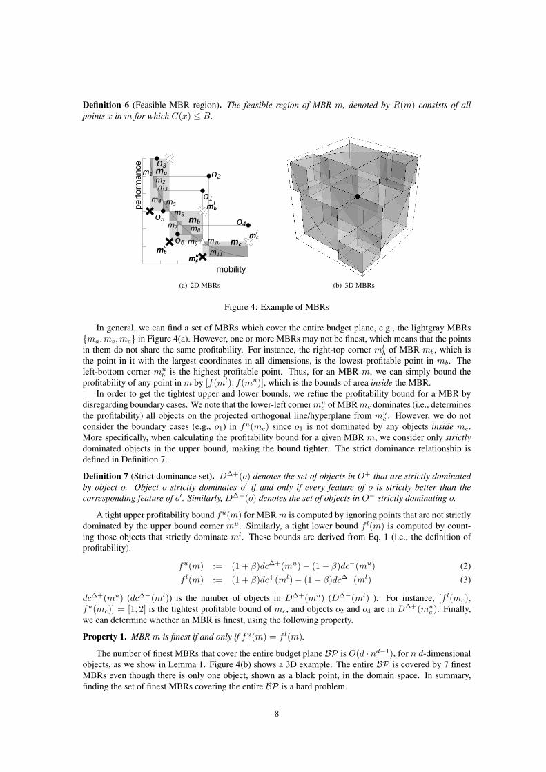
Note that a drawn hyperplane is not necessarily relevant to any MBR it intersects. Definition 8 formallyshows whether a hyperplane is relevant to an existing MBR. Broadly speaking, a hyperplane drawn fromobject o is relevant to an MBR m if the profitability of m is affected by o; i.e., o dominates some o′ ∈ mor o is dominated by some o′ ∈ m. For instance, in Figure 6, o’s hyperplane perpendicular to the y-axisintersects m1 and m2. However, it is only relevant to m1, since o is dominated by some o′ ∈ m1 but o andm2 are incomparable.

m1

m2

oBP

o's hyperplane

X

Z

Y

Figure 6: Example of relevant hyperplane

Definition 8 (Relevant hyperplane). A hyperplane from an object o is relevant to an MBR m if and only if1) the hyperplane intersectsm and 2) there is at least one point o′ inm, such that o′ dominates o if o ∈ O+

or o′ is dominated by o if o ∈ O−.

Algorithm 1 MBR Refinement Algorithmalgorithm refine(MBR setM, Budget Plane BP , Object set O)

1: for all object o ∈ O do2: M:=split(M, o, BP) . split the MBRs inM using o3: for all MBR m ∈M do4: remove m and goto line 3 if m.bu < γ5: update [m.bl,m.bu] based on o6: set γ := m.bl if γ < m.bl

7: M:=maximizeMBR(M)

Lemma 2 (Pruning). An MBRm cannot contain a region which is part of the GenBOQ solution, ifm.bu <γ, where γ = maxm∈Mm.bl andM is the set of all candidate regions.

Proof. Assume that there is a region r in m, which is part of the GenBOQ solution and m.bu < γ. Thismeans that r has higher or equal profitability than γ. Nevertheless, r ∈ m and fu(r) must be smaller thanor equal to m.bu. It contradicts our assumption, so r does not exist.

Algorithm 1 is a pseudocode of the MBR refinement algorithm. We start by initializing the result ofGenBOQ asM = {mU}, where mU is the MBR of the entire space. At every loop, we select an objecto from O and split the current set of MBRsM according to the projected lines (orthogonal hyperplanes)from o (only relevant MBRs according to Definition 8 are split). Then, we update the profitability bound[m.bl,m.bu] for every MBR m ∈ M according to the location of o. During the process, we keep track ofthe highest lower bound γ among all MBRs inM and use it to prune MBRs m for which the upper boundis smaller than γ, based on Lemma 2.

Postprocessing. Recall that during MBR refinement, the newly created MBRs are shrunk as described inAppendix A. After Algorithm 1 terminates, the MBRs which are part of the solution are not essentially the

10

largest possible. In a postprocessing step, we enlarge the MBRs (and the feasible regions inside them) suchthat no point in space having the maximum profitability is missed in the result. The enlargement processis related to the relevance concept of Definition 8. Since the profitability of an MBR is only affectedby relevant hyperplanes, the boundaries of the MBR which are not bounded by relevant hyperplanes areenlarged until the closest relevant hyperplane is met. The enlargement process does not affect correctnesssince profitability of enlarged MBRs does not change.

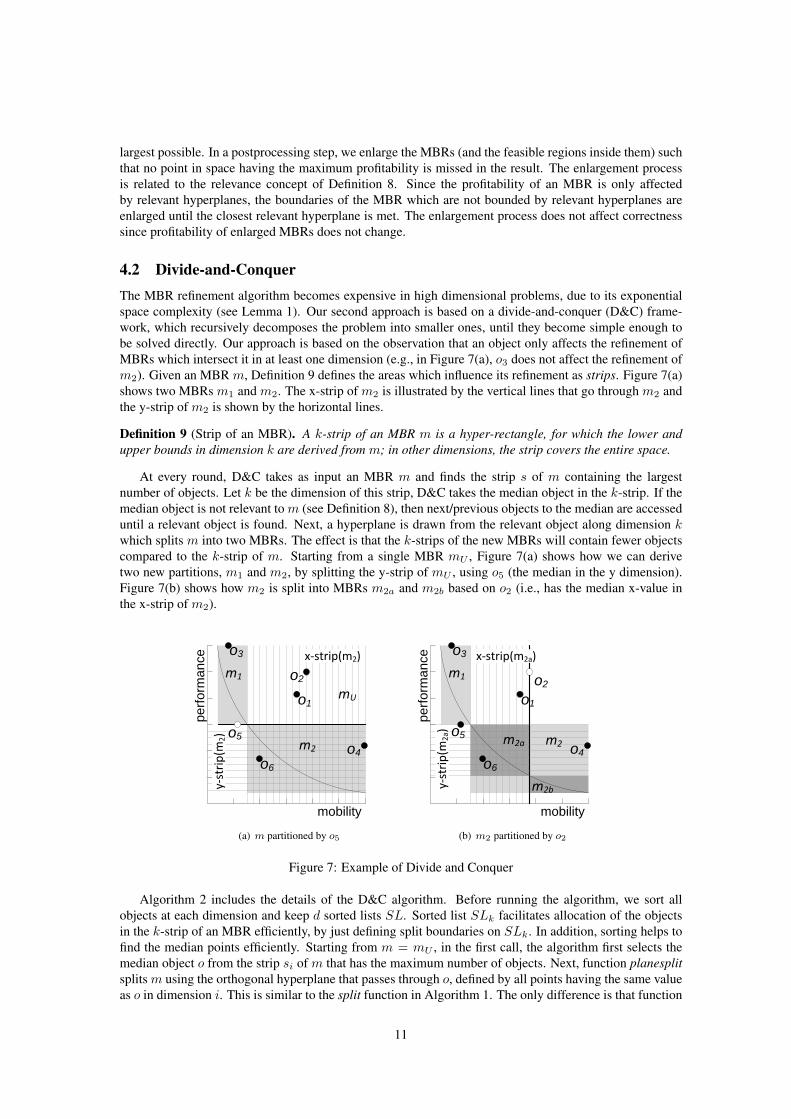
4.2 Divide-and-ConquerThe MBR refinement algorithm becomes expensive in high dimensional problems, due to its exponentialspace complexity (see Lemma 1). Our second approach is based on a divide-and-conquer (D&C) frame-work, which recursively decomposes the problem into smaller ones, until they become simple enough tobe solved directly. Our approach is based on the observation that an object only affects the refinement ofMBRs which intersect it in at least one dimension (e.g., in Figure 7(a), o3 does not affect the refinement ofm2). Given an MBR m, Definition 9 defines the areas which influence its refinement as strips. Figure 7(a)shows two MBRs m1 and m2. The x-strip of m2 is illustrated by the vertical lines that go through m2 andthe y-strip of m2 is shown by the horizontal lines.

Definition 9 (Strip of an MBR). A k-strip of an MBR m is a hyper-rectangle, for which the lower andupper bounds in dimension k are derived from m; in other dimensions, the strip covers the entire space.

At every round, D&C takes as input an MBR m and finds the strip s of m containing the largestnumber of objects. Let k be the dimension of this strip, D&C takes the median object in the k-strip. If themedian object is not relevant to m (see Definition 8), then next/previous objects to the median are accesseduntil a relevant object is found. Next, a hyperplane is drawn from the relevant object along dimension kwhich splits m into two MBRs. The effect is that the k-strips of the new MBRs will contain fewer objectscompared to the k-strip of m. Starting from a single MBR mU , Figure 7(a) shows how we can derivetwo new partitions, m1 and m2, by splitting the y-strip of mU , using o5 (the median in the y dimension).Figure 7(b) shows how m2 is split into MBRs m2a and m2b based on o2 (i.e., has the median x-value inthe x-strip of m2).

mobility

pe

rfo

rma

nce

o1

o2

x-strip(m2)

mU

o6

m2 o4

o3

m1

y-strip(m

2) o5

(a) m partitioned by o5

mobility

pe

rfo

rma

nce o3

m1

m2b

o4m2m2a

o6

o1

o2

x-strip(m2a)

y-strip(m

2a) o5

(b) m2 partitioned by o2

Figure 7: Example of Divide and Conquer

Algorithm 2 includes the details of the D&C algorithm. Before running the algorithm, we sort allobjects at each dimension and keep d sorted lists SL. Sorted list SLk facilitates allocation of the objectsin the k-strip of an MBR efficiently, by just defining split boundaries on SLk. In addition, sorting helps tofind the median points efficiently. Starting from m = mU , in the first call, the algorithm first selects themedian object o from the strip si of m that has the maximum number of objects. Next, function planesplitsplits m using the orthogonal hyperplane that passes through o, defined by all points having the same valueas o in dimension i. This is similar to the split function in Algorithm 1. The only difference is that function

11

Algorithm 2 Divide and Conquer Algorithmprerequisitefor every dimension i, objects are sorted and stored in sorted list SLialgorithm DC(partition m, Budget Plane BP)

1: select a strip si of m such that si has the maximum number of objects2: select the median object o from si using SLi3: M′:=planesplit({m}, o, i, BP)4: for all m′ ∈M′ do5: update the bound of m′ and prune m′ if it violates Lemma 26: if the total number of objects in m′’s strips < threshold θ then7: refine({m′}, BP , {all relevant objects in the strips})8: else9: DC(m′, BP)

planesplit only projects one orthogonal hyperplane instead of all hyperplanes as in function split. Forinstance, o5 projects one line to BP parallel to the x-axis but no line parallel to the y-axis in Figure 7(a).

For each of the two new MBRs m′ created by planesplit, we update the tight profitability bound of m′

by scanning all objects in the strips of m′. We decide to switch to the MBR refinement algorithm on apartition m′, if the total number of objects in all strips of m′ is smaller than a given threshold θ. Otherwise,m′ is further split by calling Algorithm 2 recursively. In this case, the refinement algorithm only accessesobjects within the strips of m′ in order to refine it to finest MBRs. Therefore, the space complexity ofcalling this method for m′ is only bounded by the number of finest MBRs in m′.

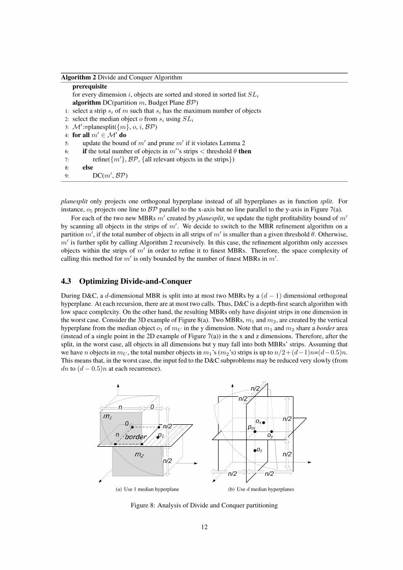
4.3 Optimizing Divide-and-Conquer

During D&C, a d-dimensional MBR is split into at most two MBRs by a (d − 1) dimensional orthogonalhyperplane. At each recursion, there are at most two calls. Thus, D&C is a depth-first search algorithm withlow space complexity. On the other hand, the resulting MBRs only have disjoint strips in one dimension inthe worst case. Consider the 3D example of Figure 8(a). Two MBRs,m1 andm2, are created by the verticalhyperplane from the median object o1 of mU in the y dimension. Note that m1 and m2 share a border area(instead of a single point in the 2D example of Figure 7(a)) in the x and z dimensions. Therefore, after thesplit, in the worst case, all objects in all dimensions but y may fall into both MBRs’ strips. Assuming thatwe have n objects inmU , the total number objects inm1’s (m2’s) strips is up to n/2+(d−1)n=(d−0.5)n.This means that, in the worst case, the input fed to the D&C subproblems may be reduced very slowly (fromdn to (d− 0.5)n at each recurrence).

n/2

0n

n/2o1

0

n

(a) Use 1 median hyperplane

n/2

oy

n/2

n/2n/2

n/2

n/2

ox

oz

pm

(b) Use d median hyperplanes

Figure 8: Analysis of Divide and Conquer partitioning

12

Avoiding the Worst Case. In order to avoid the worst case discussed above, we can adapt D&C to split thecurrent MBR m into 2d new MBRs, such that for every dimension k, if the k-strip of m has n objects, thek-strip of each new MBR m′ will have n/2 objects. This is possible if, for every dimension k, we selectthe median object in the k-strip of m and form a point pm having as coordinates these median values.The space is then split by drawing k hyperplanes perpendicular to each dimension k, passing through pm.Figure 8(b) shows a 3D example, where the three median objects ox, oy , and oz all dimensions are used toform pm, which then splits the MBR into 8 new ones, each having n/2 objects in each of its strips.

Optimization I - Optimizing Split Selection. Although the above 2d-partitioning strategy avoids theworst case, it is a pessimistic approach that will not take advantage of potential best cases. Note that thebest case of the simple D&C algorithm creates only two recurrence calls, each having only O(d · n/2)input size (i.e., all objects are partitioned equally at each dimension by one planesplit). As we show in theSection 4.5, the time complexity of such a best case is only O(d · n log(d · n)). Therefore, if a planesplitpartitions a MBR into two MBRs, such that their k-strips in all dimensions have small overlap, we performthis binary split at the D&C call; otherwise, we perform a 2d-split using pm. In the example of Figure 8(a),to assess the quality of the y-planespit based on o1, we compute the number of objects co-existing in thex-strips of m1 and m2 and sum it to the corresponding overlap in the z-strip. Dividing this number by thesum of objects in the x- and z-strips of the original MBR m, gives us an overlap ratio for the y-planespit.If this ratio is smaller than a parameter ρ, then we choose to perform the y-planesplit over the 2d-split.

Algorithm 3 Optimized Divide and Conquer Algorithmalgorithm DC(partition m, Budget Plane BP)

1: for every dimension k do2: select the median object ok from k-strip of m and update pm3: M′:=planesplit({m}, ok, k, BP)4: if overlap ratio of split is better than previous splits then5: obest:=ok; kbest:=k6: if overlap ratio of obest < ρ then7: M′:=planesplit({m}, obest, kbest, BP)8: else9: M′:=split({m}, pm, BP)

10: Run lines 4 to 9 in Algorithm 2

This version of D&C (shown as Algorithm 3) avoids the worst case, while selectively choosing binarysplits if they are favorable. For each dimension k, we find the median point of k-strip, update pm and keeptrack in kbest the dimension for which the binary split results in the minimum overlap ratio. Computingthe overlap ratio is done very efficiently by performing binary search on the corresponding sorted lists SLto identify the index of the first and last object at each dimension for the strips of m1 and m2. If the bestoverlap ratio is smaller than a given threshold ρ, we perform the corresponding planesplit, otherwise wedo a 2d split based on pm.

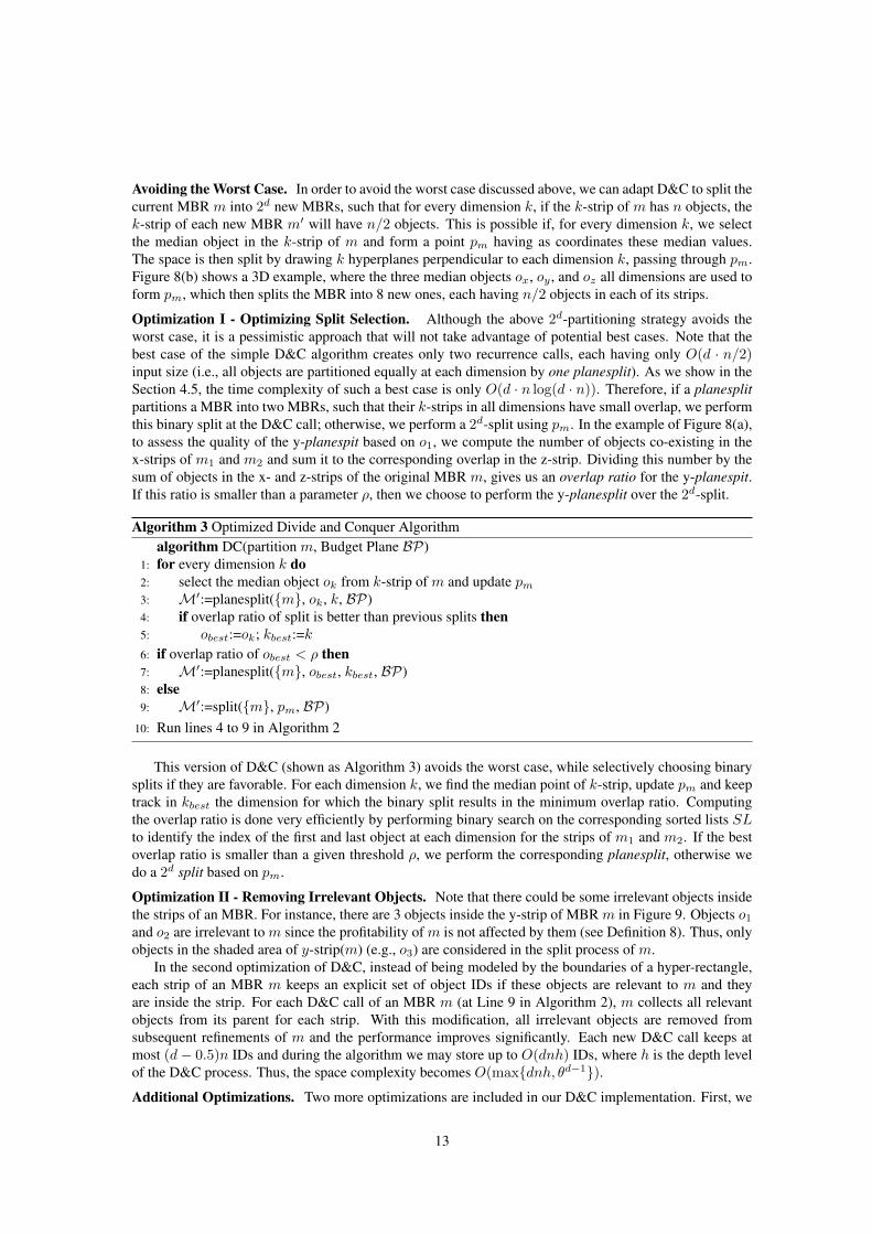
Optimization II - Removing Irrelevant Objects. Note that there could be some irrelevant objects insidethe strips of an MBR. For instance, there are 3 objects inside the y-strip of MBR m in Figure 9. Objects o1

and o2 are irrelevant to m since the profitability of m is not affected by them (see Definition 8). Thus, onlyobjects in the shaded area of y-strip(m) (e.g., o3) are considered in the split process of m.

In the second optimization of D&C, instead of being modeled by the boundaries of a hyper-rectangle,each strip of an MBR m keeps an explicit set of object IDs if these objects are relevant to m and theyare inside the strip. For each D&C call of an MBR m (at Line 9 in Algorithm 2), m collects all relevantobjects from its parent for each strip. With this modification, all irrelevant objects are removed fromsubsequent refinements of m and the performance improves significantly. Each new D&C call keeps atmost (d− 0.5)n IDs and during the algorithm we may store up to O(dnh) IDs, where h is the depth levelof the D&C process. Thus, the space complexity becomes O(max{dnh, θd−1}).

Additional Optimizations. Two more optimizations are included in our D&C implementation. First, we

13

o1

o2

o3

m

y-strip(m)

Figure 9: Example of relevant objects in a strip

observe that Lemma 2 is more effective if a better γ is found early. Based on this observation, at each D&Ccall, the generated MBRs are processed in descending order of their lower bounds mi.b

l. Second, if thereare K objects in the datasets having the same feature values, then these K objects can be grouped intoone artificial object with capacity K. The lower and upper bounds are updated according to the capacitiesof objects throughout the D&C computation. This technique is effective for real data with low-cardinalitydomains, as shown in the experimental section.

4.4 Hybrid ApproachD&C reduces the space complexity by dividing the search space recursively, in a depth-first search fashion.In this section, we explore the application of a best-first refinement (BFR) algorithm and a hybrid solutionthat combines BFR and D&C.

BFR is motivated by the observation that it is not necessary to refine the MBRs in a depth-first fashion.After refining a MBR m using one planesplit of the D&C method, the upper bounds of the resultingMBRs may be significantly smaller than that of m. In this case, it might be more promising to switchto the refinement of another MBR from those computed so far, which has higher upper bound than thenew MBRs. BFR follows such a best-first strategy for refining the MBRs. First, BFR pushes MBR mU

that covers the entire space into a heap H, which organizes the MBRs in descending order to their upperbounds. At each iteration, the MBR with the highest upper bound is deheaped, we split it using a D&Chyperplane, and the resulting MBRs are pushed back on the heap if they are not finest. The profitabilityof the best finest MBR found is used as a termination bound γ; the algorithm terminates when the nextdeheaped MBR has an upper bound which is lower than γ.

Algorithm 4 Best First Refinement Algorithmalgorithm BFR(partition m, Budget Plane BP)

1: push an MBR mU that covers the entire space into a heapH2: whileH is not empty do3: m := H.pop()4: run lines 1 to 9 in Algorithm 35: push all MBRs inM toH6: break the loop if the top MBR inH violates Lemma 2

The pseudo code of BFR is shown in Algorithm 4. BFR always chooses the currently best MBR torefine. However, this approach becomes very expensive or infeasible ifH grows beyond the memory limits(recall that the number of possible MBRs could be as high as O(d · nd−1)).

To alleviate the high memory consumption of BFR, we propose a hybrid method that combines theadvantages of BFR and D&C. A variable ω is used to control the memory usage of BFR. BFR is initiatedand used while |H| ≤ ω. As soon as |H| ≥ ω, the MBRs are accessed according to their order in H, and

14

D&C is executed for each of them to derive the finite MBRs included in them with their profitabilities. Weupdate γ and continue executing D&C for next MBR in H as long as the next MBR in H has an upperbound not smaller than γ. As we show experimentally, with a careful selection of parameter (ω), this hybridsolution can outperform D&C.

4.5 Complexity analysis

MBR Refinement Algorithm. At each step, the algorithm reads an object o and refines one or moreMBRs (e.g., m2 in Figure 5(b)). In addition, it updates the profitability bounds of one or more MBRs (e.g.,m1 and m3). Therefore, at each step we may have to update or refine all existing MBRs. In the worst case,the algorithm terminates after generating all O(d ·nd−1) finest MBRs, for a problem with n d-dimensionalobjects. The overall worst-case complexity is O(n · d · nd−1) = O(d · nd). The space complexity of thealgorithm is O(d · nd−1), as all MBRs have to be maintained and compared with the current point at eachstep.

Divide-and-Conquer. First, we analyze the computational complexity of the 2d partitioning heuristic ofD&C, which as explained has the best worst-case cost. Suppose that we have n objects, finding the medianobject o from each strip takes O(log n) time, since the objects are stored in the strip in sorted (passed fromthe previous D&C call). The most expensive step is to scan all strips of the divided MBR m and updatethe bound of each new MBR. Thus we scan O(d · n) objects in total in the d strips, and each object is usedto update the bounds of the new 2d − 1 partitions (note that one of the 2d partitions is guaranteed not tointersect BP , therefore it is pruned). Thus, the total time of a D&C call is O((2d − 1) · d · n) and eachrecursive call has O(d · n/2) input size. Note that the input size of a D&C call is d · n instead of n sincean MBR has d strips in total. By setting N = d · n, the cost of D&C can be described by the followingrecurrence.

T (N) = (2d − 1)T (N/2) +O((2d − 1)N) (4)

According to the Master Theorem [7], the bound of the recurrence function is Θ(N log(2d−1)) = Θ((d ·n)log(2d−1)). In addition, the space complexity is reduced from O(d · nd−1) to O(max{2d log d · n, |R|,θd−1}), where log d · n is the depth of the execution stack keeping 2d MBRs at each level, R is themaximum size of the candidate result set of the query, and θ is the bound used to switch to the MBRrefinement process. In summary, the worst-case time complexity is higher than that of the MBR refinementalgorithm. However, this algorithm is more efficient in practice, due to its limited space requirements.

We now analyze the best case of the algorithm. This happens when, at every call, the input MBR m ispartitioned by a planesplit equally into two MBRs, each having the input size ofm divided by 2. Therefore,the cost of D&C in the best case can be described by the following recurrence.

T (N) = 2T (N/2) +O(2N) (5)

By applying Master Theorem [7], the bound of the recurrence is Θ(N logN) = Θ((d · n) log(d · n)). Asdiscussed in Section 4.3, the optimized D&C method would prefer good binary splits to 2d splits if theyresult in good partitions.

5 Approximation of GenBOQBased on our D&C framework, we propose a method which returns an approximate GenBOQ result witha quality guarantee. Instead of computing all feasible regions in GenBOQ, our approximation solution(ApprGenBOQ) returns only one feasible region rappr such that the profitability of rappr is bounded by atolerance T from the optimal. Formally:

Problem 3 (Approximation of GenBOQ). (APPRGEN-BOQ) Consider a budget B, a constraint functionC(x), and an objective function f(x). Let R be the (optimal) regions returned by GenBOQ. ApprGenBOQreturns any region rappr such that, ∀x ∈ R,∀y ∈ rappr, we have |f(x) − f(y)| ≤ T where T is a givenquality tolerance bound.

15

D&C based approximation. Based on the definition, the MBR returned by the approximate methoddoes not have to be finest due to the tolerance bound T . Thus, an MBR is a potential result only if the gapbetween its upper and lower profitability bounds is smaller than T . Formally:

Definition 10 (Qualified MBR). An MBR m is a potential result of ApprGenBOQ if m.bu −m.bl ≤ T .

In the D&C framework, we iteratively split an MBR if the number of objects in the MBR’s strips islarger than a threshold θ. Otherwise, we refine the MBR by Algorithm 1. For the approximation solution, ifan MBR is qualified, it is not necessary to split/refine it further. However, a qualified MBR is not necessarya result of ApprGenBOQ. We use Definition 11 to compare two qualified MBRs and eventually find aqualified MBR that is a result.

Definition 11 (Comparison of qualified MBRs). We say qualified MBR m1 is better than qualified MBRm2 if and only if m1.b

u > m2.bu.

In Lemma 3, we show that the best among all qualified MBRs (according to Definition 11) must be aresult of ApprGenBOQ. Note that we return only one qualified MBR in ApprGenBOQ. Therefore, if theupper bound of a new created MBR m′ is not larger than the maximum upper bound η of the qualifiedregions found so far, then m′ can be pruned safely. In summary, once we compute a qualified MBR, theMBR is either kept as a result candidate or pruned by η.

Lemma 3 (Correctness of approximation). A qualified MBR m is a result of ApprGenBOQ if m.bu ≥ η,where η = maxm∈Mqual

m.bu andMqual is the set of qualified MBRs.

Proof. Suppose that the maximum profitability is p. So our task is to prove that p ∈ [m.bl,m.bu].

• If p < m.bl, then there must exist a profitability p′ = f(x) better than p, where x ∈ m. Thiscontradicts the assumption that p is the maximum profitability.

• If p > m.bu, then we must have another MBR m′ where p ∈ [m′.bl,m′.bu], which means m.bu <p ≤ m′.bu, so m should be pruned according to Definition 11. This contradicts the fact that m is thelast result candidate.

Algorithm 5 Divide and Conquer Approximation Algorithmalgorithm DCAppr(partition m, Budget Plane BP , tolerance T )

1: Run lines 1 to 9 in Algorithm 32: for all m′ ∈M′ do3: update the bound of m′

4: prune m′ if it violates Lemma 2 or m′.bu < η5: if m′.bu −m′.bl ≤ T then6: set m′ as the result candidate7: else if the total number of objects in m′’s strips < threshold θ then8: refineAppr({m′}, BP , {all relevant objects in the strips})9: update result candidate

10: else11: DCAppr(m′, BP , T )12: return result candidate

Algorithm 5 (extended from Algorithm 3) is a pseudocode of our approximation solution. For eachnewly created MBR m′, we first test whether m′ can be pruned or not (Line 4). If m′ is not prunedand m′ is a qualified MBR, then m′ is set as the result candidate. If m′ is not a qualified MBR, m′ iseither refined or split by corresponding processes. Note that, during the MBR refinement process, we stoprefining MBRs once they become qualified. Accordingly, function refineAppr in Line 8 is used to represent

16

the modified version of Algorithm 1. After the refinement process, we may update the result candidatefrom the newly qualified MBRs (Line 9). Note that our approximation solution is directly applicable to thehybrid approach.

6 Experimental EvaluationWe empirically evaluate the performance of the proposed algorithms: the MBR refinement algorithm (M-BR) (Section 4.1), divide-and-conquer (D&C) (Section 4.2), the hybrid approach (Section 4.4), and theapproximation method (Section 5).

Three types of synthetic datasets, independent (IND), correlated (COR), and anti-correlated (ANT),are generated according to the methodology in [5]. In IND datasets, the feature values are generated u-niformly and independently. COR datasets contain objects whose values are correlated in all dimensions.ANT datasets contain objects whose values are good in one dimension and tend to be poor in other di-mensions. In addition, we generate cluster (CLU) datasets by randomly selecting ξ independent objects,and treat them as cluster centers. Each cluster object is generated by a Gaussian distribution with mean atthe selected cluster center and standard deviation 5% of each dimension domain range. We set ξ to 10 bydefault. The above four types of data are common benchmarks for skyline queries [5, 23]. Our dataspacecontains d dimensions (in the range from 2 to 5). Additionally, we experiment with two real datasets,Household [3] and NBA [1].

By default, we use one type of constraint function, C(x) = 1Π1≤i≤d(x[i]) , which gives equal weights

to all dimensions, in order not to bias any attribute. In general, the constraint function is designed by adomain expert. In addition, we also evaluate an alternative function, composed by a set of linear functions.

All methods were implemented in C++ and the experiments were performed on an Intel Core2Duo2.66GHz CPU machine with 4 GBytes memory, running on Ubuntu 9.04. Table 2 shows the ranges of theinvestigated parameters, and their default values (in bold). In each experiment, we vary a single parameter,while setting the others to their default values. For each method, we measure the total execution time,including any preprocessing costs, and the peak memory usage. As we will show shortly, after tuning ofparameters θ (refinement threshold) and ρ (overlap ratio), they are set to their best values (10 and 0.7,respectively), throughout all remaining experiments.

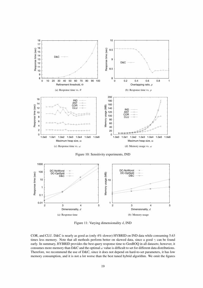
Parameter Tuning. We first study the effect of the various tuning parameters on the algorithms. Weinvestigate the effect of θ (Section 4.2) and the overlap ratio ρ (Section 4.3). Figure 10(a) shows theeffect of θ on the cost of the D&C algorithm on the default IND dataset. For very small values of θ, therefinement process becomes very fast; however, there are also more D&C recurrence calls. For very largeθ, the execution time is high due to the expensive refinement process. Also, the memory usage becomeshigher; the peak number of MBRs created by the refinement process at θ = 100 is 21541 while it is only 35and 169 at θ = 10 and θ = 20 respectively. The best overall value in terms of response time is in between5 to 20, so we choose θ = 10 as the default value in order to reduce the number of D&C recurrence calls.

Next, we test the effect of the overlap ratio ρ on the D&C algorithm. As Figure 10(b) shows, the costtrend of D&C agrees with our discussion in Section 4.3. D&C becomes more expensive when we only use2d splits (ρ = 0) since it does not take advantage of possible best cases. Its execution time is 15% higherthan our default ratio ρ = 0.7.

We also study the effect of the maximum heap size ω on the hybrid solution. Figures 10(c) and 10(d)show the response time and memory usage of different data distributions as a function of ω. For ω = 0,hybrid becomes plain D&C; on the other hand, as ω increases, hybrid becomes more like BFR. COR andCLU datasets favor the BFR approach since the data are more skewed and a good γ can be computed early.For IND and ANT datasets it is more difficult to find a good ω value, since the points on the budget planehave similar profitabilities and a good bound to prune large MBRs is hard to find. For all data distributions,the memory usage increases with ω. We set ω to 5120 since it gives the minimum value for all datadistributions, regardless of the large memory consumption compared to plain D&C method.

Effectiveness of Optimizations. Next, we evaluate the effectiveness of the optimizations proposed inSection 4.3 within the D&C algorithm. The fully optimized algorithm (D&C) is compared against D&C-NoWorst (the divide-and-conquer algorithm with all 2d splits, described in Section 4.3 Avoiding the Worst

17

Table 2: Range of parameter valuesParameter Values

|O| (in thousand) 10, 25, 50, 100, 200

Dimensionality d 2, 3, 4, 5

Data distribution IND, ANT, COR, CLU

Overlap ratio ρ 0, 0.05, 0.1, ..., 0.7, ..., 0.95, 1

Refinement threshold θ 2, 5, 10, 20, 40, 80

Maximum heap size ω 0, 2, 5, 10, 20, ..., 5120, ..., 81920, 163840Number of clusters ξ 10, 50, 100, 200,..., 1600

Constraint function C(o)(a) 1

Π1≤i≤d(o[i])

(b) max

1

α·o[1]+∑

1≤i≤d,i6=1 o[i]

...1

α·o[d]+∑

1≤i≤d,i6=d o[i]

Development budget B 2, 5, 10, 100, 1000, 10000, 100000

α 0.1, 0.2, 0.4, 0.8, 1.6, 3.2

Quality T/|O| 0.01%, 0.05%, 0.1%, 0.5%, 1%, 2%, 5%

Discrete values (DADA) 5, 7, 10, 12, 15, 17, 20

Case) and D&C-OptSplit (the basic divide-and-conquer algorithm with optimized split selection, describedin Section 4.3 Optimizing Split Selection).

Figure 11 plots the response time and memory usage of the three D&C versions as a function of thedimensionality d, after setting all other parameters to their default values. The response time increasesexponentially in all methods, but fully optimized D&C is less sensitive to dimensionality than the othermethods. It is 3.30 and 2.70 times faster than D&C-NoWorst and D&C-OptSplit for d = 5, while consum-ing at most 46% more memory. Note that D&C-NoWorst and D&C-OptSplit are faster than the D&C atd = 2, since the computation in this case is very fast and the optimization for irrelevant objects pruningcomes with a significant cost factor.

Scalability experiments. Next, we compare the proposed solutions (D&C and hybrid) to the naivemethod (MBR). Two versions of the hybrid method are evaluated. In HYBRID, ω is set to 5120 based onour tuning. HYBRID-Max is used to test BFR when ω is set to a large number (ω = 163, 840).

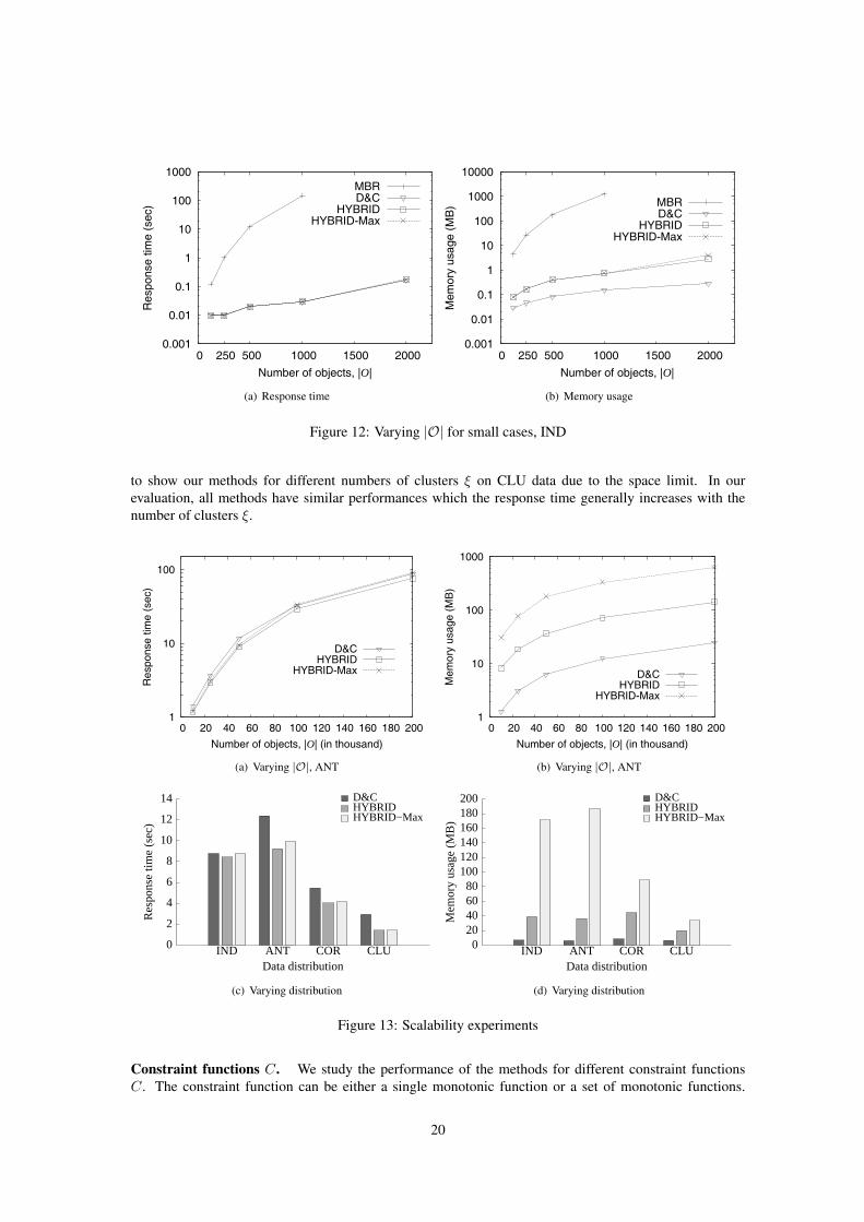
Because the memory usage of the baseline method MBR grows exponentially with the dimensionality,we only test it on a small dataset with |O| ranging from 125 to 2000, for d = 4. As shown in Figure 12,the cost of MBR grows very fast. When |O| = 2000, the space requirements of MBR exceed the availablememory. The cost of the other methods grows exponentially, as well, but at a much lower pace than thenaive approach. Their memory usage increases at even lower pace. This demonstrates that our approachesare a substantial contribution, since this is a very expensive problem even for small datasets.

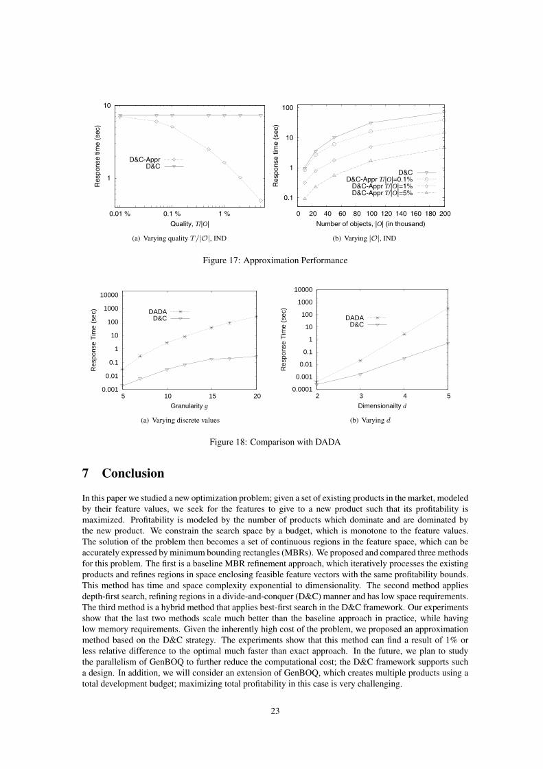
In the remaining experiments, we exclude the baseline method (MBR), due to its high cost. Figure13(a) shows the response time of the remaining methods as a function of the number of objects on anti-correlated data. HYBRID is 14.9% (19.9%) faster than D&C (HYBRID-Max) at |O| = 200K. However,HYBRID consumes more memory than D&C (at least 5.7 times) due to the heap structure. More pre-cisely, it consumes 72.24 MB (142.75 MB) for |O| = 100K (|O| = 200K), while D&C consumes only12.54 MB (25.05 MB). HYBRID-Max is not only slower but also consumes more memory (633.64 MB at|O| = 200K) than the others. The memory usage of all methods increases linearly with |O|, as shown inFigure 13(b).

Figures 13(c) and 13(d) show the response time and memory usage of the methods on different datadistributions. HYBRID is the best method in terms of response time in all four data distributions IND, ANT,

18

8

9

10

11

12

13

14

15

16

17

18

0 10 20 30 40 50 60 70 80 90 100

Res

pons

e tim

e (s

ec)

Refinement threshold, Θ

D&C

(a) Response time vs. θ

8

8.5

9

9.5

10

0 0.2 0.4 0.6 0.8 1

Res

pons

e tim

e (s

ec)

Overlapping ratio, ρ

D&C

(b) Response time vs. ρ

0

2

4

6

8

10

12

14

16

1.0e0 1.0e1 1.0e2 1.0e3 1.0e4 1.0e5 1.0e6

Res

pons

e tim

e (s

ec)

Maximum heap size, ω

INDANTCORCLU

(c) Response time vs. ω

0

20

40

60

80

100

120

140

160

180

200

1.0e0 1.0e1 1.0e2 1.0e3 1.0e4 1.0e5 1.0e6

Mem

ory

usag

e (M

B)

Maximum heap size, ω

INDANTCORCLU

(d) Memory usage vs. ω

Figure 10: Sensitivity experiments, IND

0.01

0.1

1

10

100

1000

2 3 4 5

Res

pons

e tim

e (s

ec)

Dimensionality, d

DC-NoWorstDC-OptSplit

D&C

(a) Response time

1

10

2 3 4 5

Mem

ory

usag

e (M

B)

Dimensionality, d

DC-NoWorstDC-OptSplit

D&C

(b) Memory usage

Figure 11: Varying dimensionality d, IND

COR, and CLU. D&C is nearly as good as (only 4% slower) HYBRID on IND data while consuming 5.63times less memory. Note that all methods perform better on skewed data, since a good γ can be foundearly. In summary, HYBRID provides the best query response time to GenBOQ in all datasets; however, itconsumes more memory than D&C and the optimal ω value is difficult to set for different data distributions.Therefore, we recommend the use of D&C, since it does not depend on hard-to-set parameters, it has lowmemory consumption, and it is not a lot worse than the best tuned hybrid algorithm. We omit the figures

19

0.001

0.01

0.1

1

10

100

1000

0 250 500 1000 1500 2000

Res

pons

e tim

e (s

ec)

Number of objects, |O|

MBRD&C

HYBRIDHYBRID-Max

(a) Response time

0.001

0.01

0.1

1

10

100

1000

10000

0 250 500 1000 1500 2000

Mem

ory

usag

e (M

B)

Number of objects, |O|

MBRD&C

HYBRIDHYBRID-Max

(b) Memory usage

Figure 12: Varying |O| for small cases, IND

to show our methods for different numbers of clusters ξ on CLU data due to the space limit. In ourevaluation, all methods have similar performances which the response time generally increases with thenumber of clusters ξ.

1

10

100

0 20 40 60 80 100 120 140 160 180 200

Res

pons

e tim

e (s

ec)

Number of objects, |O| (in thousand)

D&CHYBRID

HYBRID-Max

(a) Varying |O|, ANT

1

10

100

1000

0 20 40 60 80 100 120 140 160 180 200

Mem

ory

usag

e (M

B)

Number of objects, |O| (in thousand)

D&CHYBRID

HYBRID-Max

(b) Varying |O|, ANT

D&CHYBRIDHYBRID−Max

0

2

4

6

8

10

12

14

IND ANT COR CLU

Res

pons

e tim

e (s

ec)

Data distribution

(c) Varying distribution

D&CHYBRIDHYBRID−Max

0 20 40 60 80

100 120 140 160 180 200

IND ANT COR CLU

Mem

ory

usag

e (M

B)

Data distribution

(d) Varying distribution

Figure 13: Scalability experiments

Constraint functions C. We study the performance of the methods for different constraint functionsC. The constraint function can be either a single monotonic function or a set of monotonic functions.

20

Figure 14(a) plots the response time of the solutions with respect to the budget B of a type-a function(C(o) = 1

Π1≤i≤d(o[i]) = B) on correlated datasets (COR). For very small or very large values of B, theproblem becomes easier on COR datasets since the budget plane BP is close to left-bottom or right-topcorner of the space. Hybrid methods outperform D&C on COR datasets.

We also evaluated the performance of type-b constraint functions (a set of linear functions) defined inTable 2 on IND datasets. For each linear function lfi, we set all coefficients to 1 except i-th coefficient; thei-th coefficient is set to α. Besides, we set B = 1 in order to avoid negative profitability results such thatthe size of positive object set O+ is larger than negative object set O− on these two datasets. As Figure14(b) shows, the problem is easier to solve at α = 0.1 and α = 3.2, for the same reason as in small andlarge values ofB in type-a constraint functions. Like in type-a functions, hybrid methods outperform D&Con independent datasets.

0.1

1

10

1 10 100 1000 10000 100000

Res

pons

e tim

e (s

ec)

Development budget, B

D&CHYBRID

HYBRID-Max

(a) Varying B on type-a, COR

0

5

10

15

20

25

0 0.5 1 1.5 2 2.5 3 3.5

Res

pons

e tim

e (s

ec)

α

D&CHYBRID

HYBRID-Max

(b) Varying α on type-b, IND

Figure 14: Varying on different constraint function types C

Data distribution. We also evaluated our methods for different numbers of clusters ξ on CLU data.Figure 15 demonstrates the response time and memory usage of all methods as a function of ξ. All threemethods have similar performances which the response time generally increases with the number of clus-ters. HYBRID is the best method except at ξ = 1600 since the ω value of HYBRID is no longer optimized.

1

10

0 200 400 600 800 1000 1200 1400 1600

Res

pons

e tim

e (s

ec)

Number of clusters, ξ

D&CHYBRID

HYBRID-Max

(a) Response time

1

10

100

1000

0 200 400 600 800 1000 1200 1400 1600

Mem

ory

usag

e (M

B)

Number of clusters, ξ

D&CHYBRID

HYBRID-Max

(b) Memory usage

Figure 15: Varying on number of clusters, ξ

Real data. NBA contains 12,278 statistics from regular seasons during 1973-2008, each of which cor-responds to the statistics of an NBA player’s performance in 6 aspects (minutes played, points, rebounds,assists, steals, and blocks). Household consists of 3.6M records during 2003-2006, each representing thepercentage of an American family’s annual expenses on 4 types of expenditures (electricity, water, gas, and

21

property insurance). In the following experiments, we exclude HYBRID-Max due to its bad performance interms of response time and memory usage. To avoid negative profitability results, we set the developmentbudget B to 1M.

Figure 16(a) shows the response time of three methods (MBR, D&C, and HYBRID) as a function ofdimensionality. The response time of all methods increases exponentially to the dimensionality. D&C andHYBRID have similar response time due to small data size. Again, MBR exceeds the available memorywhen d ≥ 3, so it is only included for d = 2; in this case MBR is 2 orders of magnitude slower than ourproposed methods.

Figure 16(b) compares the response time of D&C and HYBRID with their variants D&C\CAP andHYBRID\CAP that exclude the capacity optimization described in Section 4.3. We divided Householdinto four datasets with 516K, 514K, 1.25M, and 1.35M records from years 2003, 2004, 2005, and 2006respectively. The feature values in Household are discrete, so there are some tuples having the same featurevalues in all dimensions; in this case the objects are grouped to a single capacitated object. The numberof discrete objects are 242K, 250K, 520K, and 542K, respectively in the four years. The fully optimizedmethods are significantly faster than the methods that do not apply capacity optimization. HYBRID isfaster than D&C in all tests since the Household dataset is highly clustered; this is also the reason why allmethods perform better on the Household dataset than the synthetic datasets.

0.01

0.1

1

10

100

1000

2 3 4 5 6

Res

pons

e tim

e (s

ec)

Dimensionality, D

MBRD&C

HYBRID

(a) NBA

D&C\CAPD&CHYBRID\CAPHYBRID

0

2

4

6

8

10

12

2,003 2,004 2,005 2,006

Res

pons

e tim

e (s

ec)

Year

(b) Household

Figure 16: Results with Real Datasets

Approximation. We use the ratio of tolerance bound T divided by the number of objects |O| to representthe quality of an approximation result. We first evaluate the response time of our approximation approachas a function of quality, showing the response time of D&C as a baseline. Figure 17(a) shows that theresponse time of D&C-Appr decreases dramatically with the increase of T . At the default quality setting(T/|O| = 1%), D&C-Appr is 4.5 times faster than D&C, showing that D&C-Appr finds a result efficientlywithout sacrificing much precision. Figure 17(b) tests the scalability of D&C-Appr, showing the responsetime of four methods (D&C and three quality settings of D&C-Appr) as a function of the number of objects.All D&C-Appr methods are consistently faster than D&C. Moreover, D&C-Appr with T/|O| = 1% is 4.86times faster than D&C for O = 200K. Thus, the performance gain of D&C-Appr is not affected by theproblem size.

DADA. Finally, we test the efficiency of our approach against DADA [11]. We generate datasets, where thefeature values of objects are discrete for every dimension, so that both LOQ in DADA and GenBOQ returnthe same result. For each dataset, we construct the D*-tree index for LOQ. In Figure 18(a) and Figure 18(b),we show the response time of LOQ (excluding the time to construct the D*-tree) and our D&C approach.D&C outperforms DADA by 1 to 3 orders of magnitude, and this superiority increases when we increasethe number of discrete values or the dimensionality. This demonstrates why our method is more generalthan DADA, since it can be applied to continuous or discrete feature spaces of large cardinalities.

22

1

10

0.01 % 0.1 % 1 %

Res

pons

e tim

e (s

ec)

Quality, T/|O|

D&C-ApprD&C

(a) Varying quality T/|O|, IND

0.1

1

10

100

0 20 40 60 80 100 120 140 160 180 200

Res

pons

e tim

e (s

ec)

Number of objects, |O| (in thousand)

D&CD&C-Appr T/|O|=0.1%

D&C-Appr T/|O|=1%D&C-Appr T/|O|=5%

(b) Varying |O|, IND

Figure 17: Approximation Performance

0.001

0.01

0.1

1

10

100

1000

10000

5 10 15 20

Res

pons

e T

ime

(sec

)

Granularity g

DADAD&C

(a) Varying discrete values

0.0001

0.001

0.01

0.1

1

10

100

1000

10000

2 3 4 5

Res

pons

e T

ime

(sec

)

Dimensionailty d

DADAD&C

(b) Varying d

Figure 18: Comparison with DADA

7 Conclusion

In this paper we studied a new optimization problem; given a set of existing products in the market, modeledby their feature values, we seek for the features to give to a new product such that its profitability ismaximized. Profitability is modeled by the number of products which dominate and are dominated bythe new product. We constrain the search space by a budget, which is monotone to the feature values.The solution of the problem then becomes a set of continuous regions in the feature space, which can beaccurately expressed by minimum bounding rectangles (MBRs). We proposed and compared three methodsfor this problem. The first is a baseline MBR refinement approach, which iteratively processes the existingproducts and refines regions in space enclosing feasible feature vectors with the same profitability bounds.This method has time and space complexity exponential to dimensionality. The second method appliesdepth-first search, refining regions in a divide-and-conquer (D&C) manner and has low space requirements.The third method is a hybrid method that applies best-first search in the D&C framework. Our experimentsshow that the last two methods scale much better than the baseline approach in practice, while havinglow memory requirements. Given the inherently high cost of the problem, we proposed an approximationmethod based on the D&C strategy. The experiments show that this method can find a result of 1% orless relative difference to the optimal much faster than exact approach. In the future, we plan to studythe parallelism of GenBOQ to further reduce the computational cost; the D&C framework supports sucha design. In addition, we will consider an extension of GenBOQ, which creates multiple products using atotal development budget; maximizing total profitability in this case is very challenging.

23

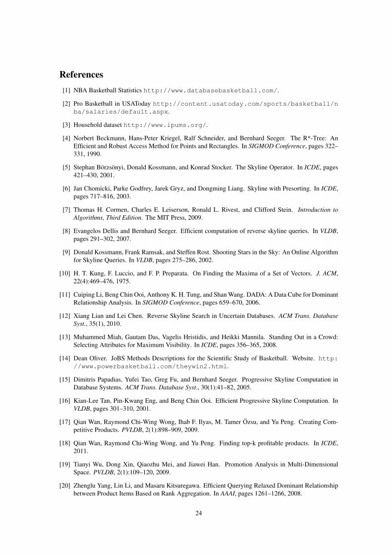
References[1] NBA Basketball Statistics http://www.databasebasketball.com/.

[2] Pro Basketball in USAToday http://content.usatoday.com/sports/basketball/nba/salaries/default.aspx.

[3] Household dataset http://www.ipums.org/.

[4] Norbert Beckmann, Hans-Peter Kriegel, Ralf Schneider, and Bernhard Seeger. The R*-Tree: AnEfficient and Robust Access Method for Points and Rectangles. In SIGMOD Conference, pages 322–331, 1990.

[5] Stephan Borzsonyi, Donald Kossmann, and Konrad Stocker. The Skyline Operator. In ICDE, pages421–430, 2001.

[6] Jan Chomicki, Parke Godfrey, Jarek Gryz, and Dongming Liang. Skyline with Presorting. In ICDE,pages 717–816, 2003.

[7] Thomas H. Cormen, Charles E. Leiserson, Ronald L. Rivest, and Clifford Stein. Introduction toAlgorithms, Third Edition. The MIT Press, 2009.

[8] Evangelos Dellis and Bernhard Seeger. Efficient computation of reverse skyline queries. In VLDB,pages 291–302, 2007.

[9] Donald Kossmann, Frank Ramsak, and Steffen Rost. Shooting Stars in the Sky: An Online Algorithmfor Skyline Queries. In VLDB, pages 275–286, 2002.

[10] H. T. Kung, F. Luccio, and F. P. Preparata. On Finding the Maxima of a Set of Vectors. J. ACM,22(4):469–476, 1975.

[11] Cuiping Li, Beng Chin Ooi, Anthony K. H. Tung, and Shan Wang. DADA: A Data Cube for DominantRelationship Analysis. In SIGMOD Conference, pages 659–670, 2006.

[12] Xiang Lian and Lei Chen. Reverse Skyline Search in Uncertain Databases. ACM Trans. DatabaseSyst., 35(1), 2010.

[13] Muhammed Miah, Gautam Das, Vagelis Hristidis, and Heikki Mannila. Standing Out in a Crowd:Selecting Attributes for Maximum Visibility. In ICDE, pages 356–365, 2008.

[14] Dean Oliver. JoBS Methods Descriptions for the Scientific Study of Basketball. Website. http://www.powerbasketball.com/theywin2.html.

[15] Dimitris Papadias, Yufei Tao, Greg Fu, and Bernhard Seeger. Progressive Skyline Computation inDatabase Systems. ACM Trans. Database Syst., 30(1):41–82, 2005.

[16] Kian-Lee Tan, Pin-Kwang Eng, and Beng Chin Ooi. Efficient Progressive Skyline Computation. InVLDB, pages 301–310, 2001.

[17] Qian Wan, Raymond Chi-Wing Wong, Ihab F. Ilyas, M. Tamer Ozsu, and Yu Peng. Creating Com-petitive Products. PVLDB, 2(1):898–909, 2009.

[18] Qian Wan, Raymond Chi-Wing Wong, and Yu Peng. Finding top-k profitable products. In ICDE,2011.

[19] Tianyi Wu, Dong Xin, Qiaozhu Mei, and Jiawei Han. Promotion Analysis in Multi-DimensionalSpace. PVLDB, 2(1):109–120, 2009.

[20] Zhenglu Yang, Lin Li, and Masaru Kitsuregawa. Efficient Querying Relaxed Dominant Relationshipbetween Product Items Based on Rank Aggregation. In AAAI, pages 1261–1266, 2008.

24

[21] Zhenglu Yang, Botao Wang, and Masaru Kitsuregawa. General Dominant Relationship AnalysisBased on Partial Order Models. In SAC, pages 470–474, 2007.

[22] Man Lung Yiu and Nikos Mamoulis. Multi-dimensional Top-k Dominating Queries. VLDB J.,18(3):695–718, 2009.

[23] Shiming Zhang, Nikos Mamoulis, and David W. Cheung. Scalable Skyline Computation UsingObject-based Space Partitioning. In SIGMOD Conference, pages 483–494, 2009.

[24] Zhenjie Zhang, Laks V. S. Lakshmanan, and Anthony K. H. Tung. On Domination Game Analysisfor Microeconomic Data Mining. TKDD, 2(4), 2009.

APPENDIX

A Compact MBR ComputationGiven an MBRm, a budget plane BP , and an orthogonal hyperplane, we can partitionm into (at most) twocompact MBRs as shown in Figure 8(a). In this section, we show how we can compute the boundaries ofthese new MBRs in O(d2) time. For the sake of presentation, we assume that the hyperplane splits m intoexactly two MBRs m1 and m2. Assume that m is split by hyperplane x[j] = v (i.e., parallel to dimensionj at value v). Let ml[i] (mu[i]) be the lower (upper) bound of m in dimension i. Then, two loose MBRs,whose union equals m can be defined by the following equations.

ml1 := ml mu

1 [i] :=

{mu[i] if i 6= j

v if i = j(6)

ml2[i] :=

{ml[i] if i 6= j

v if i = jmu

2 := mu (7)

Note that the values of mu1 and ml

2 are the tightest values already; in addition, ml1[j] and mu

2 [j] are alsotightest. However, we can tighten the values (ml

1 and mu2 ) in other dimensions, so that m1 and m2 tightly

enclose BP using the following method. To find the maximum bound within an MBR in dimension i, weneed to set the minimum values in all other dimensions and solve C(x) = B. For example, ml

1[i] can becomputed by solving the equation C(x) = B, by setting x[j] = mu

1 [j],∀j 6= i.

Figure 19: Compact MBR Computation

For instance, in Figure 19, assume that we want to partition m using hyperplane y= 0.5. Initially, mis split into two MBRs m1 = {mu

1 ,ml1} = {[0, 0.5], [1, 1]} and m2 = {mu

2 ,ml2} = {[0, 0], [1, 0.5]}.

Then, if C = 1x[0]x[1] and B = 0.5, we tighten ml

1[0] by solving ml1[0] · mu

1 [1] = B, which gives

25

ml1[0] = 0.5/0.5 = 0.25. Therefore, the tight-most bound of m1 becomes {[0, 0.5], [0.25, 1]}. In general,

d− 1 boundaries can be tightened for each new MBR and each tightening requires O(d) computations, sothe overall cost for tightening an MBR is O(d2).

26