University of Nebraska - Lincoln University of Nebraska - Lincoln

DigitalCommons@University of Nebraska - Lincoln DigitalCommons@University of Nebraska - Lincoln

Biological Systems Engineering--Dissertations, Theses, and Student Research Biological Systems Engineering

5-2020

Application of an Ultrasonic Sensor to Monitor Soil Erosion and Application of an Ultrasonic Sensor to Monitor Soil Erosion and

Deposition Deposition

Jessica E. Johnson University of Nebraska - Lincoln, johnson.jessie@huskers.unl.edu

Follow this and additional works at: https://digitalcommons.unl.edu/biosysengdiss

Part of the Bioresource and Agricultural Engineering Commons

Johnson, Jessica E., "Application of an Ultrasonic Sensor to Monitor Soil Erosion and Deposition" (2020). Biological Systems Engineering--Dissertations, Theses, and Student Research. 103. https://digitalcommons.unl.edu/biosysengdiss/103

This Article is brought to you for free and open access by the Biological Systems Engineering at DigitalCommons@University of Nebraska - Lincoln. It has been accepted for inclusion in Biological Systems Engineering--Dissertations, Theses, and Student Research by an authorized administrator of DigitalCommons@University of Nebraska - Lincoln.

APPLICATION OF AN ULTRASONIC SENSOR TO MONITOR SOIL EROSION

AND DEPOSITION

by

Jessica E. Johnson

A THESIS

Presented to the Faculty of

The Graduate College at the University of Nebraska

In Partial Fulfillment of Requirements

For the Degree of Master of Science

Major: Agricultural and Biological Systems Engineering

Under the Supervision of Professors Aaron Mittelstet and Nancy Shank

Lincoln, Nebraska

May, 2020

APPLICATION OF AN ULTRASONIC SENSOR TO MONITOR SOIL EROSION

AND DEPOSITION

Jessica E. Johnson, M.S.

University of Nebraska, 2020

Advisors: Aaron Mittelstet and Nancy Shank

While erosion and deposition are naturally occurring processes, these processes

can be accelerated by human influences. The acceleration of erosion causes damage to

human assets and costs billions of dollars to mitigate. Monitoring erosion at high

resolutions can provide researchers and managers the data necessary to help manage

erosion. Current erosion monitoring methods tend to be invasive to the area, record low

frequency measurements, have a narrow spatial range of measurement, or are very

expensive. There is a need for an affordable monitoring system capable of monitoring

erosion and deposition non-invasively at a high resolution. The objectives of this research

were to (1) design and construct a non-invasive sediment monitoring system (SMS) using

an ultrasonic sensor capable of monitoring erosion and deposition continuously, (2) test

the system in the lab and field, (3) and determine the applications and limitations of the

system. The ultrasonic sensor measures the time of reflectance of sound waves to

calculate the distance to the area non-invasively. The SMS was tested in the lab to

determine the extent to which the soil type, slope, surface topography, change in distance

and vegetation impact the SMS’s ultrasonic sensor’s measurement. It was found that the

soil type, slope and surface topography had little effect on the measurement, but the

change in distance of the measurement and the introduction of vegetation impacted the

measurement. The error in measurement increased as the sensing distance increased, and

vegetation interferes with the measurement. In the field during high flows, as erosion and

deposition occur, the changes in distance were determined in near real-time, allowing for

the calculation of erosion and deposition quantities. The system was deployed to monitor

deposition on sandy streambanks in the Nebraska Sandhills and erosion on a streambank

and field plot in Lincoln, Nebraska. The system was proven successful in measuring

sediment change during high flow events but yielded some error; ±1.06 mm in controlled

lab settings and ±10.79 mm when subjected to environmental factors such as temperature,

relative humidity and wind.

iii

Table of Contents

CHAPTER 1: INTRODUCTION .................................................................................... 1

Erosion and Deposition Background............................................................................... 1

Review of Erosion and Deposition Monitoring Methods ............................................... 5

Study Objectives ............................................................................................................. 8

CHAPTER 2: MATERIALS AND METHODS .......................................................... 10

Development of Sediment Monitoring System ............................................................. 10

Laboratory Controlled Experiments .............................................................................. 13

Field Experiments ......................................................................................................... 15

Study Sites ..................................................................................................................... 15

Data Analysis ................................................................................................................ 19

CHAPTER 3: RESULTS AND DISCUSSION ............................................................ 20

Control Experiments ..................................................................................................... 20

Field Experiments ......................................................................................................... 22

CHAPTER 4: RESILIENCE, POLICY AND OUTREACH IN RIPARIAN

ECOSYSTEMS ............................................................................................................... 34

CHAPTER 5: CONCLUSTIONS AND FUTURE WORK ........................................ 39

REFERENCES ................................................................................................................ 41

APPENDIX A: USER GUIDE ....................................................................................... 44

APPENDIX B: WIRING GUIDE .................................................................................. 47

APPENDIX C: CODE .................................................................................................... 49

iv

List of Tables and Figures

Figure 2.1: SMS’s electronic components and ultrasonic sensor ..................................... 12

Figure 2.2: Control experimental set ups .......................................................................... 14

Figure 2.3: Field site experimental set ups ....................................................................... 18

Figure 3.1: Control results for sediment and distance changes ........................................ 21

Figure 3.2: Control results for surface topography and vegetation impacts ..................... 22

Figure 3.3: Field sites results ............................................................................................ 23

Figure 3.4: Flooding event results from Sand Draw Creek .............................................. 32

Table 3.1: Bank pin data from SBMLR ............................................................................ 25

Table 3.2: Bank pin data from Sand Draw Creek ............................................................. 26

1

CHAPTER 1: INTRODUCTION

Erosion and Deposition Background

Erosion and deposition are naturally occurring processes that occur along the

banks of rivers and streams, constantly shaping the channel. They also occur in rangeland

and agricultural fields. While erosion occurs in some degree across all landscapes, not all

erosion occurs at the same rate. There are two types of erosion: geological erosion and

accelerated erosion. Geological erosion occurs slowly overtime and is responsible for soil

formation, distribution and topographical feature creation like stream channels.

Accelerated erosion is human or animal induced by the removal of natural vegetation and

leads to the breakdown of soil and accelerates the removal of organic and mineral

particles (Schwab, Fangmeier, & Elliot, 1996). Erosion reduces the productivity of

agricultural lands due to soil and nutrient loss. Agricultural practices accelerate the loss

of nutrients and soil at a far greater rate than it can be replenished through natural

processes (Amundson, et al., 2015). In order to maintain productive agricultural lands to

feed the world’s growing population, extensive resources are spent to recuperate lost

productivity from soil degradation and the subsequent polluting of waterways. Annually,

$44 billion is spent in the U.S. on erosion damage and control (Pimentel, et al., 1995) and

the more than $1 billion on stream restoration (Bernhardt, 2005). Incorporating

conservation practices into agricultural production was reported to reduce soil loss in

South America by as much as 16% and in North America by as much as 12.5% (Borrelli,

et al., 2017).

In order to manage areas with erosion problems, it is important to understand the

factors that influence erosion. The main factors that affect soil erosion are climate, soil

2

type, vegetation and topography (Schwab, Fangmeier, & Elliot, 1996). Climatic factors

that affect erosion are mainly precipitation and wind; the rainfall energy and intensity

influence the amount of erosion seen in a runoff producing rainstorm and wind can

transport finer soil particles and cause significant erosion with winds of 20 to 30

kilometers per hour (FAO, Soil erosion by wind, 1978) and (Department of Environment

and Resource Management, 2011). The physical properties of the soil also influence

erosion; soil structure, texture, density and water content. The detachment of soil

particles tends to increase as soil particles become coarser, but the transport of the soil

particle increases with finer particles (FAO, Soil Erosion by water, 1978). Basically, sand

particles can detach easier because they are coarser and allow water to penetrate them

easier, but smaller clay particles transport easier (once detached) because they are a finer

particle. There are three important effects vegetation has on soil erosion (1) protection of

soil surface from direct rainfall to reduce runoff, (2) reduction of soil movement due to

rooting of the vegetation, and (3) plant transpiration reduces the water content of the soil

and probability of runoff. The final factor affecting soil erosion is the topography of the

area. The degree of slope, shape, length of slope and watershed area. Steeper slopes

produce runoff that is more erosive and transports sediments downhill easier (Schwab,

Fangmeier, & Elliot, 1996).

Water erosion can cause four different types of erosion: splash, sheet, rill and

gully erosion. Splash erosion is caused by the direct impact of water droplets from

rainfall or irrigation striking the soil surface and displacing and washing away soil

particles. Sheet erosion occurs when runoff washes a layer of soil from an entire field/

slope area. Humans have a hard time perceiving splash and sheet erosion due to the fine

3

scales with which they remove sediment. Rill and gully erosion are much more

pronounced and visible forms of erosion. Rill erosion occurs when enough runoff moves

across a surface to cause small channels to form. As rill erosion progresses, channels

become deeper and ultimately leads to gully erosion. Gully erosion is one of the most

destructive forms of erosion as the runoff tends to concentrate in the gullies and enhance

erosion rates. Gullies generally continue to grow as sediment is lost from the side walls,

unless control measures are implemented to reduce and prevent erosion (Carey, 2006).

Gully erosion can be attributed to as much as 80% of the total sediment production in a

watershed while only making up approximately 1-5% of the area (Poesen, Nachtergaele,

Verstraeten, & Valentin, 2003). Water erosion models tend to only include sheet and rill

erosion and not gully erosion (Poesen, 2017). Gully erosion models are limited due to the

little knowledge surrounding how gullies start, develop and infill in different

environments and how they interact with other hydrological processes like infiltration,

drainage and recharge to groundwater (Poesen, 2011). There is also no standardized

method to monitor gully erosion rates and there is a lack of quality data to calibrate and

validate the few models that do attempt to model gully erosion (Poesen, 2017).

The management of erosion depends on accurate and reliable data. Data that is

long-term, continuous, accurate, and reliable are essential to quantify the timing and

amount of erosion. The management of erosion depends on accurate and reliable data. In

some cases, erosion is measured qualitatively by visual observation of erosion and

classified as either none, slight, moderate or severe (Lal, 1994). It is difficult to determine

quantitative amounts of erosion from these classifications. Without proper or with

inaccurate measured erosion quantities, models cannot be developed and validated to

4

predict erosion amounts. Erosion models are useful for management and policy decisions

to understand future impacts of erosion processes.

One model that is used frequently for modeling streambank erosion and retreat is

the Bank Stability and Toe Erosion Model (BSTEM). There have been few studies done

evaluating BSTEM against long-term streambank erosion data. Using long-term erosion

data with the BSTEM model can help identify which parameters are the most important

for estimating streambank erosion and retreat (Midgley, Fox, & Heeren, 2012). The use

of long-term and high frequency erosion data would provide even greater input into

which parameters are most important and help to solidify the timing of erosion during the

streambank retreat process. While Midgley et al. (2012) was able to closely predict the

timing of erosion events in their study, they did not use continuous data, so their

measurements occurred days to weeks after high flow events leaving uncertainty in their

predictions of timing. Continuous erosion data would allow for the reduction in

uncertainty of the prediction of the timing and could help identify the controlling

parameters around those events. Calibration and validation of models, like BSTEM,

would also be enhanced from having long-term, large scale, and high frequency erosion

data (Poesen, 2017). Accurate predictions of erosion are essential for natural resource

managers so they can manage areas that are most at-risk from erosion like crop fields and

streambanks.

BSTEM also has the capability to model different stabilization techniques,

making it an important tool for the management of streambank erosion. BSTEM is a

process-based method that has the potential to determine the bank response, predicts

initial and final sediment loads and bank retreat rates, to erosion control measures and

5

aids in the design of bank stabilization practices (Klavon, et al., 2017). While BSTEM

can be used as an important tool for mitigating erosion problems, the model has

limitations and could benefit from quality, long-term streambank erosion data to validate

the model and enhance model processes. Enhancing the model would make is more

broadly applicable and accessible to managers allowing for better streambank

stabilization practices to be implemented.

Review of Erosion and Deposition Monitoring Methods

There are a variety of methods and devices used to measure sediment changes

(i.e. soil erosion or deposition). One conventional method is bank pins, which are stakes

that are inserted into the area of interest (AOI) in a gridded pattern and measured over

time to document the total quantity of sediment change (Thorne, 1981). Another

traditional method is surveying techniques, which is the repeated measurement or survey

of the bank width to document the location of the bank and its retreat (erosion) over time

(Lawler, 1993 and Thorne, 1981). A more modern technique is the use of Photo-electric

erosion pins (PEEP) which uses photovoltaic cells in series to sense incident light and

outputs a signal, recorded continuously, proportional to the amount of rod exposed

(Lawler, 2001). While PEEPs are typically installed to monitor erosion, they are also

capable of monitoring deposition as well. Other monitoring systems include

LiDAR/Terrestrial Laser Scanning (TLS) and satellite or drone imagery. LiDAR uses

laser pulses and the measured reflected pulse to calculate the distance from sensor to

bank surface. The lasers are sometimes mounted on a pan-tilt motor so the bank can be

scanned, and sediment changes calculated (Plenner, Eichinger, & Bettis, 2016 and Lague,

Brodu, & Leroux, 2013). The analysis of images from earth orbiting satellites or UAVs

6

(Cook, 2017) can also provide information on bank retreat and sediment changes. While

most methods are deployed to monitor erosion, each has the capability to monitor

deposition as well, except for surveying techniques as these tend to just monitor bank

retreat. Aerial imagery analysis is also limited on monitoring deposition but Cook (2017)

was able to quantify certain amounts of deposition as well as erosion. The following

review of literature analyzes these different monitoring methods’ frequency of

measurement, scale of measurement, invasiveness to the measurement area, and

affordability.

Of the six erosion monitoring methods reviewed, only half of them record data at

a high frequency, while the others only provide data as often as the user manually

conducts the measurement. The bank pins, stream surveys and satellite/ drone imagery

are limited in their ability to perform high frequency measurements. Bank pins and

stream surveys are simple to use and give accurate measurements of the total quantity of

soil lost or gained, but they are labor intensive as each measurement requires additional

visits to the study site (Thorne, 198 and Lawler, 1993). Finally, analysis of aerial imagery

from UAVs or satellite provide a slightly higher frequency than bank pins or surveys, but

are still limited by the frequency in which images can be taken (Cook, 2017). Each of

these methods result in erosion measurements at a low temporal resolution and are unable

to provide the timing of the erosional event (rainstorm) that caused the erosion.

The photo-electric erosion pins (PEEP) and LiDAR/ TLS both provide high

frequency measurements. While these methods provide data at a high frequency there is

variability in the consistency of the measurements. PEEP devices only have a high

frequency in measurement during the day as the device is unusable at night without

7

incident light to indicate the amount of exposed pin (Lawler, 2001). While not restricted

by time of day, the TLS lacks consistency with length of time being deployed in the field.

According to Plenner et al. (2016) the TLS was unable to capture bank profiles

immediately after storm events because it was only used during low flow. Also due to the

cost of the equipment, the device was only used during certain times and not left to

monitor the bank continuously. This reduces the frequency in measurement and leaves

knowledge gaps of erosion-causing events.

Quantifying sediment change not only means having continuous and accurate

data, but data that is measured from a large area to understand the dynamics of the bank

movement. Conventional methods were classified into two types of measurements, point

measurements and bank measurements. The bank pins and PEEP devices are point

measurements because data is only measured at the point of the pin. The LiDAR/TLS and

aerial imagery can measure the sediment change of the whole bank. The TLS was

mounted on a pan-tilt motor to scan the entire bank to measure the bank profile (Plenner,

Eichinger, & Bettis, 2016). Aerial imagery can capture the change of a whole bank or

changes over the area from taking multiple photos of the whole area, but the resolution of

the data is variable. Cook (2017) found that there was 30 to 40 cm of variation between

the affordable UAV images and analysis compared to that of the LiDAR system used to

measure the same sediment changes. Drones designed for photogrammetry, which are

typically pricy, can reduce this error but are still limited by photo resolution and analysis

techniques (Lague, Brodu, & Leroux, 2013).

Bank pins and PEEP devices can be used in a gridded pattern to capture sediment

change data over a larger area, but this can result in reduced bank stability due to the

8

concentration of pins that must be inserted into the area which may influence the

sediment change observed (Lawler, 2001). PEEPs are also particularly invasive due to the

cables that also have to be dug into the bank for their operation and the vegetation that

must be removed so direct light can strike the PEEP surface (Lawler, 1991 and Lawler,

2001). In order to reduce the influence of the monitoring technique on the AOI, the

technique must be non-invasive. LiDAR/TLS and aerial imagery analysis are both non-

invasive techniques to monitor sediment change. Imagery taken by UAV and satellites

can observe the AOI from above and will not influence the area. Similarly, most LiDAR/

TLS systems are set a distance away from the AOI and observed remotely by using the

time of reflectance of light pulses.

Study Objectives

From the review above, the most accurate, non-invasive, continuous monitoring

device is the LiDAR/ TLS systems. While these systems do provide quality erosion data,

they tend to be very expensive. Plenner et al. (2016) created an “affordable” TLS system

for approximately $10,000. In order for multiple devices to be used for extended periods

of time they must have significantly lower costs. As discussed, current erosion

monitoring methods tend to be either invasive to the area, record low frequency

measurements, have a narrow spatial range of measurement, or are very expensive. Thus,

there is a need for an affordable monitoring system capable of monitoring erosion and

deposition non-invasively at a high resolution. Objectives of this research were to (1)

design and construct a non-invasive sediment monitoring system capable of monitoring

erosion/ deposition continuously (2) test the system in the lab and field, (3) and determine

the applications and limitations of the system. These objectives were met by utilizing

9

ultrasonic sensors in conjunction with programmable electronics to develop a continuous,

non-invasive erosion and deposition monitoring device for approximately $350.

10

CHAPTER 2: MATERIALS AND METHODS

Development of Sediment Monitoring System

The sediment monitoring system (SMS) consisted of the following components:

ultrasonic sensor, Arduino Nano, data storage electronics, compact battery and

temperature probe. The most important piece of equipment was the ultrasonic sensor of

which we chose the MaxBotix HRXL-MaxSonar-WR MB7389. The sensor uses the

principle of time of flight to determine range to the surface. A sound wave is emitted in

the direction of the surface. Once the sound wave strikes the surface, part of the sound

wave bounces back and is detected by the sensor. The time between emittance and

detection is used in combination with the speed of sound to calculate the distance to the

surface by the following equation.

𝐷 = 𝑣𝑡 (1)

where D is the distance to the surface (m), v is the speed of sound (m/s) and t is the time

of flight in seconds. The sensor determines the range to the largest object in the AOI

(Maxbotix, HRXL-MaxSonar ®-WR ™ Series, 2012). When erosion or deposition occur,

the sensor will measure the new distance to the AOI, thus enabling the quantity of erosion

or deposition to be calculated. Erosion or deposition will have to occur over the majority

of the area, nearly half, to be the largest object to be recorded by the sensor. The sensor is

also designed to detect hard surface targets instead of soft surface targets, making it less

susceptible to vegetation and rainfall influences. While the sound waves can penetrate

vegetation and rainfall, these factors could still impact the sensors measuring capability.

The ultrasonic sensor monitors an area of 2,826 cm2 as it has a circular beam

pattern with a radius of 30 cm. This beam is dependent on the distance from the sensor.

When within 30 cm, the sensor is unable to record the distance to the AOI as there is too

11

much interference between the emitted and reflected sound wave. Outside of 30 cm the

sensor maintains the 30 cm radius beam out to its maximum range. Our study utilized two

sensors, with maximum ranges of five (HRXL-MaxSonar-WR MB7389) and ten meters

(XL-MaxSonar-WRML MB7051).

In addition to the sensor’s maximum range, there is also inherent error in the

sensor’s measurement. The manufacturer states an error of approximately 1% of the total

sensing distance; this correlates to a ± 1 cm error range when sensing at a distance of 1

m. Measuring greater distances will therefore increase the error up to ±10 cm for the 10

m sensor. Along with the instrumental error inherent in the sensor as reported by the

manufacturer, the speed of sound is impacted by environmental factors like temperature,

relative humidity and wind (Bohn, 1988; Chen & Maher, 2004; and Ingard, 1953).

The distance measured by the ultrasonic sensor is recorded by routing the sensor’s

serial output to an Arduino Nano, which boots, initiates 50 measurements, records the

median value of the measurements and timestamp on a SD card unit, and returns the

system to sleep mode to save battery life when not taking measurements. The frequency

of measurement (interval for sleep mode) and data filter can be changed within the

Arduino code. For this study the frequency of measurement was set to 15 minutes. A

deep-cycle 12-volt, 22 amp-hour battery was used to power the system approximately

one month (28 days). The date and time are kept by the real-time clock (RTC) module

which is connected to the Arduino Nano and logged to a 32-gigabyte microSD card held

in the SD card module when the sensor takes a measurement. The electronics and battery

were encased in a water resistant, weatherproof box to protect the unit from

environmental conditions while deployed in the field (Figure 2.1).

12

Figure 2.1 Components of the sediment monitoring system including the system

electronics (Arduino Nano and RTC) and SD Card with module which are installed in

weatherproof box and the 5 m ultrasonic sensor.

Also included in the monitoring system is an external temperature probe

(MaxTemp) to correct the speed of sound for the current air temperature. In order to meet

the National Weather Service (2018) recommendations for accurate measuring of air

temperature, the temperature probe was mounted on the bottom side of the weatherproof

electronics and battery housing box so it would be in a shaded and well-ventilated area.

The temperature probe was connected directly to the ultrasonic sensor which

automatically adjusted the speed of sound for the recorded air temperature to calculate

the distance to the AOI by the following equation:

𝐷 = 𝑇𝑂𝐹20.05 √𝑇𝑐+273.15

2 (2)

where D is the distance (m), TOF is the time of flight (s), and Tc is the air temperature

(⁰C). The temperature operation range of the MaxSonar ultrasonic sensor is -40C to

13

+65C, well within average daily temperature ranges (Maxbotix, Temperature

Compensation Report).

Laboratory Controlled Experiments

The erosion monitoring system was first tested in a controlled lab setting (Figure

2.2a) to evaluate the manufacturer’s error specifications and determine the impact of

multiple variables that may influence the distance measured by the sensor. The

experiment was carried out in a secluded area (closet) to reduce any influence from

external factors. The control box and battery were placed on a counter and the ultrasonic

sensor was mounted on a ring stand facing down at a pan containing soil. The dimensions

of the soil pan measured approximately 60 cm length by 45 cm width. The width is less

than the ultrasonic sensor’s beam width, but the sensor measures the largest object in its

field of view which was determined to be the soil pan since changes in the soil were

measured by the sensor. Changes made during the control tests were confirmed by

manually measuring the distance from the sensor to the soil to determine the artificial

erosion and deposition amounts and distance changes in the different experiments

conducted.

In order to determine the factors that influence and limit the SMS, investigations

into different factors were conducted to help determine the extent to which they may

influence the measurement. A total of seven scenarios were evaluated: erosion,

deposition, slope, surface topography, soil type, vegetation and distance. Each

experiment, except when testing multiple distances, were conducted with the ultrasonic

sensor remaining stationary in the same location (approximately 1.25 m away). The first

experiment investigated the SMS’s capability of monitoring erosion. Approximately 2.2

14

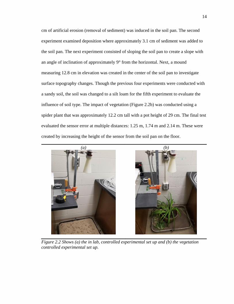
cm of artificial erosion (removal of sediment) was induced in the soil pan. The second

experiment examined deposition where approximately 3.1 cm of sediment was added to

the soil pan. The next experiment consisted of sloping the soil pan to create a slope with

an angle of inclination of approximately 9° from the horizontal. Next, a mound

measuring 12.8 cm in elevation was created in the center of the soil pan to investigate

surface topography changes. Though the previous four experiments were conducted with

a sandy soil, the soil was changed to a silt loam for the fifth experiment to evaluate the

influence of soil type. The impact of vegetation (Figure 2.2b) was conducted using a

spider plant that was approximately 12.2 cm tall with a pot height of 29 cm. The final test

evaluated the sensor error at multiple distances: 1.25 m, 1.74 m and 2.14 m. These were

created by increasing the height of the sensor from the soil pan on the floor.

(a)

(b)

Figure 2.2 Shows (a) the in lab, controlled experimental set up and (b) the vegetation

controlled experimental set up.

15

Field Experiments

Once the system was tested in the lab, four SMS’s were installed at four study

sites to monitor deposition on the inside of a meander (2), field erosion (1), and

streambank erosion on the outside of a meander (1). Sediment deposition was monitored

at two sites in the Nebraska Sandhills, the South Branch of the Middle Loup River

(SBMLR) and Sand Draw Creek. Field erosion was monitored at a UNL research facility,

Roger’s Memorial Farm, east of Lincoln, NE. Streambank erosion was monitored on

Beal Slough, a tributary to Salt Creek in Lincoln, NE.

Study Sites

The SMS was set up on a sandy stream bank on the SBMLR located within the

Gudmundsen Sandhill’s Laboratory (GSL). The facility, owned by the University of

Nebraska-Lincoln, is a research ranch located in the heart of the Sandhills in western

Nebraska. The Sandhills, dominated by sandy soils, is a dynamic system with erosion and

deposition common during high flow events. The SMS was mounted on a horizontal arm

facing downward to, non-invasively, monitor deposition (Figure 2.3a) along the stream

bank opposite of a cut bank suffering from mass wasting events. The stream ran through

a pasture; therefore, to protect the AOI and equipment from cattle rubbing, a fence was

installed. While the system was able to monitor non-invasively, bank pins (Thorne, 1981)

were used to confirm erosion/ deposition amounts occurring in the AOI. Four pins were

inserted into the ground, each located 40 cm from the center of the AOI, outside of the

ultrasonic sensor’s sensing area. During each visit to the site, the bank pins were

measured along with the distance from the sensor to the ground to act as a ghost bank pin

for the center of the AOI. Site visits occurred approximately every 28 days to replace the

16

battery, download the system’s data and record the bank pins. The SMS was deployed

from the beginning of October to the end of November. The water height of these streams

was monitored to compare the timing of sediment altering events to those captured by the

monitoring system. The water and barometric pressure, converted to water depth, were

measured using HOBO pressure transducers.

Sand Draw Creek is a small tributary to the Niobrara River in north central

Nebraska. The study site is located near Ainsworth, NE in Brown County and is in the

Middle Niobrara Natural Resource District. Although this stream is located on the edge

of the Sandhills, the predominant soil type is still sand. The SMS was installed in a

privately owned pasture with cattle grazing occurring during the monitoring time. Like

the study site located on SBMLR, a fence was set up around the AOI and monitoring

system to protect it from cattle. The ultrasonic sensor was mounted on a horizontal arm

and faced downward to monitor deposition (Figure 2.3b). Bank pins were also installed to

track the deposition and HOBO pressure transducers were used to monitor the stream

depth to compare with deposition events. The system was set up from August until

September when a large flooding event destroyed the system. The new system was then

re-installed from the beginning of October until the end of November and checked

approximately every 28 days to replace the battery and record the bank pin information.

Roger’s Memorial Farm is a research farm owned and operated by the University

of Nebraska-Lincoln for conducting research experiments on agriculture lands. The farm

has historically been a no-till farm and uses terraces on the sloping fields to help control

sediment loss. The dominate soil type is a silty clay loam which has slow infiltration

rates. Evidence of past erosion can be seen before the use of no-till and terrace practices

17

(Nebraska-Lincoln, 2020). This farm was not expected to produce many, if any, erosional

events due to its management but was used due to its proximity to campus and the appeal

of testing the sensor in a different setting. The sensor was mounted on a horizontal arm

and pointed downward to monitor a small patch of slightly sloped ground that had been

tilled for a microplastics study; this was to increase the possibility of catching an erosion

event. The non-invasiveness of the system (Figure 2.3c) was paramount to not interfere

with the other scientific study being conducted on that area; consequently, erosion pins

were not used at this site, but manual measurements from the sensor to ground

measurements were conducted. This system was set up from the beginning of September

2019 to early spring 2020; with an updated temperature probe being installed on October

14th.

The final system that was deployed was in the south part of Lincoln, NE on a

large cut bank causing erosion near a high voltage power pole on the urban waterway

Beal Slough. The system was mounted on the cut bank to monitor erosion (Figure 2.3d).

The original design was for the SMS to monitor streambank erosion from the bank

opposite of the AOI. Due to the range constraints of the ultrasonic sensor, an extended

cable was attached to the ultrasonic sensor so it could monitor erosion from the same

bank but set back a couple meters to avoid interference or damage from erosion forces.

The cable was run through a 2.4 m pipe staked to the ground which over hung the eroding

bank. The sensor was then mounted to a 1.2 m pipe protruding vertically down from the

overhanging pipe (see Appendix A: Figure A.1a). Due to the limited accessibility to the

large and steep cut bank, erosion pins were not used at this site and manual sensor to AOI

measurements were unable to be conducted. Like the sites located in the Sandhills, a

18

HOBO pressure transducer was used to monitor the stream depth. This SMS was

deployed from mid-October 2019 to January 2020. This site was unique due to its

location in an urban area, likelihood of receiving flashy runoff, and due to its monitoring

of at-risk infrastructure.

(a)

(b)

(c)

(d)

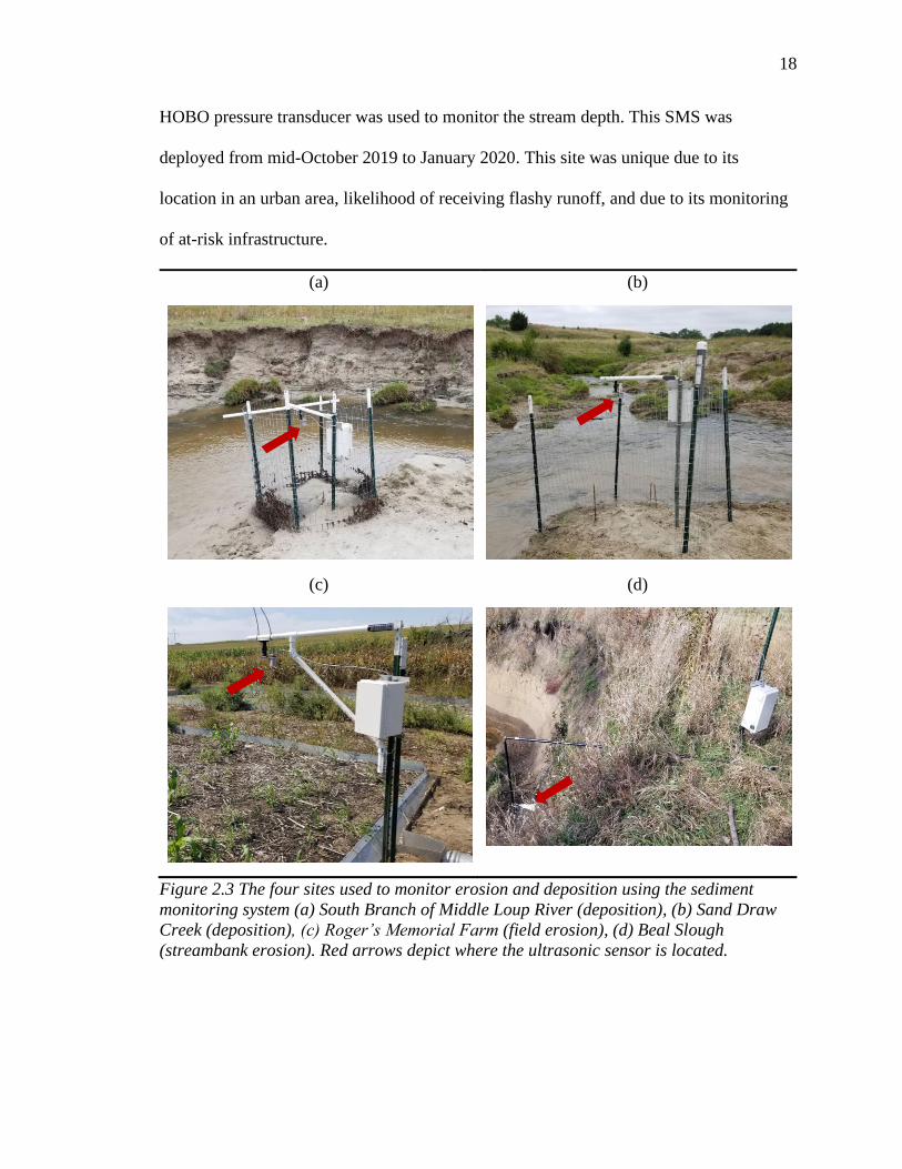
Figure 2.3 The four sites used to monitor erosion and deposition using the sediment

monitoring system (a) South Branch of Middle Loup River (deposition), (b) Sand Draw

Creek (deposition), (c) Roger’s Memorial Farm (field erosion), (d) Beal Slough

(streambank erosion). Red arrows depict where the ultrasonic sensor is located.

19

Data Analysis

Data was analyzed using Excel and R. Plots were constructed illustrating the

measured distances against the date-time values to determine where and how much

erosion or deposition occurred. Water level was also plotted, where applicable, to help

determine when events occurred that would cause erosion or deposition. Once events

were determined, the raw data for each event at each site was processed using the R data

language. Outliers were removed based on box plot statistics with outliers lying outside

the inner fences (NIST, n.d.). Once outliers were removed, the daily median value was

determined to help smooth the data and reduce the noise of the measurement. The

standard deviation was then calculated for each event to determine the error range of the

measurement. Finally, plots were reconstructed with the filtered and smoothed data and

water level data to quantify and show when erosional or depositional events occurred.

20

CHAPTER 3: RESULTS AND DISCUSSION

Control Experiments

The laboratory-controlled testing helped to evaluate potential factors that would

affect the results of the SMS. Initially, erosion and deposition were tested using a sandy

soil. Figure 3.1a shows the different artificial erosion and deposition events that were

created. The SMS recorded a 23 mm change, with an error of ± 0.979 mm, from BASE to

ERO, indicating approximately 2.3 cm of erosion. This compares to the approximate 2.2

cm of actual erosion created. Similarly, there was 29 ± 0.945 mm of deposition from

ERO to DEP which is comparable to the approximate 3.1 cm of actual deposition

created. These findings confirm that the SMS accurately measures erosion and deposition

events.

Figure 3.1b illustrates the results from testing the system at approximately 1.25 m

(X), 1.72 m (Y) and 2.14 m (Z). The variation was ±1.06 mm for 1.25 m and then

increased as the distance increased. At 1.74 m and 2.14 m the variation was ±4.66 mm

and ±8.02 mm respectively, which is within the manufacturers stated 1% error of the

distance measured. Due to the increases in the variation of the measurement over longer

distances, field studies were conducted to keep the ultrasonic sensor ~1 m away from the

AOI. This would provide limited variation in measurement while still being non-invasive.

21

(a)

(b)

Figure 3.1 Results from the controlled experiments in the lab. Plot (a) Shows the control

BASE, an artificial erosion event ERO, and an artificial deposition event DEP. (b)

Shows the differences in height X at 1.25 m, Y at 1.74 m and Z at 2.14 m. Note that most

of the measured distance measurements occur at the same distance as the median filtered

data and are hard to denote behind the median filtered line.

After the effects of multiple distances were evaluated, changes in the topography

were investigated. Figure 3.2a shows the results of the sloped and mounded experiments.

The variation in measurement of the sloped experiment was ±1.28 mm and the mounded

experiment had a variation of ±1.18 mm. The sensor read to the top of the mound, nearest

target, during the experiment. This suggests that small changes in surface topography

does not have a significant impact on the error in the measurement; however, it is

important to note that steeper slopes could create more error in measurement and that the

sensor will only measure the nearest target so the whole sensing area will be assumed to

have similar sediment change.

Figure 3.2b provides the results of the change in soil type to a silt loam and the

vegetation experiments. The silt loam soil had a variation in measurement of ±1.00 mm

which is comparable with the variation of error of the sandy soil of ±1.06 mm, both

experiments were conducted at approximately 1.25 m. Therefore, the SMS should

22

provide accurate results across different soil types. The spider plant was measured, with a

ruler, to be 121.92 mm tall and the SMS records a change in distance of approximately

123.50 mm between the start of the experiment to the end. This suggests that the system

was picking up the plant near the beginning of the experiment and then sound waves

were able to penetrate the vegetation and the distance to the soil in the pot was recorded.

These results indicate that vegetation is an important factor that can influence the reading

of the sensor. The impacts of the vegetation on readings was seen in the field during the

beginning of the study period at the Roger’s Memorial Farm.

(a)

(b)

Figure 3.2 shows the results from the controlled experiments in the lab. Plot (a) shows

the sloped SL and mounded MD experimental results. (b) Shows the silt loam soil type

SLS and the vegetation trial VEG with a spider plant placed above the silt loam soil.

Field Experiments

After controlled experiments were conducted, the SMS was tested in the field. For

the system monitoring deposition on the SBMLR, there was slight water level fluctuation

and little sediment change observed by the SMS during the beginning of the monitoring

period (October 2nd to October 28th) (Figure 3.3a). This confirms that the SMS was able

to provide stable readings during a time when there were no major changes in the AOI.

23

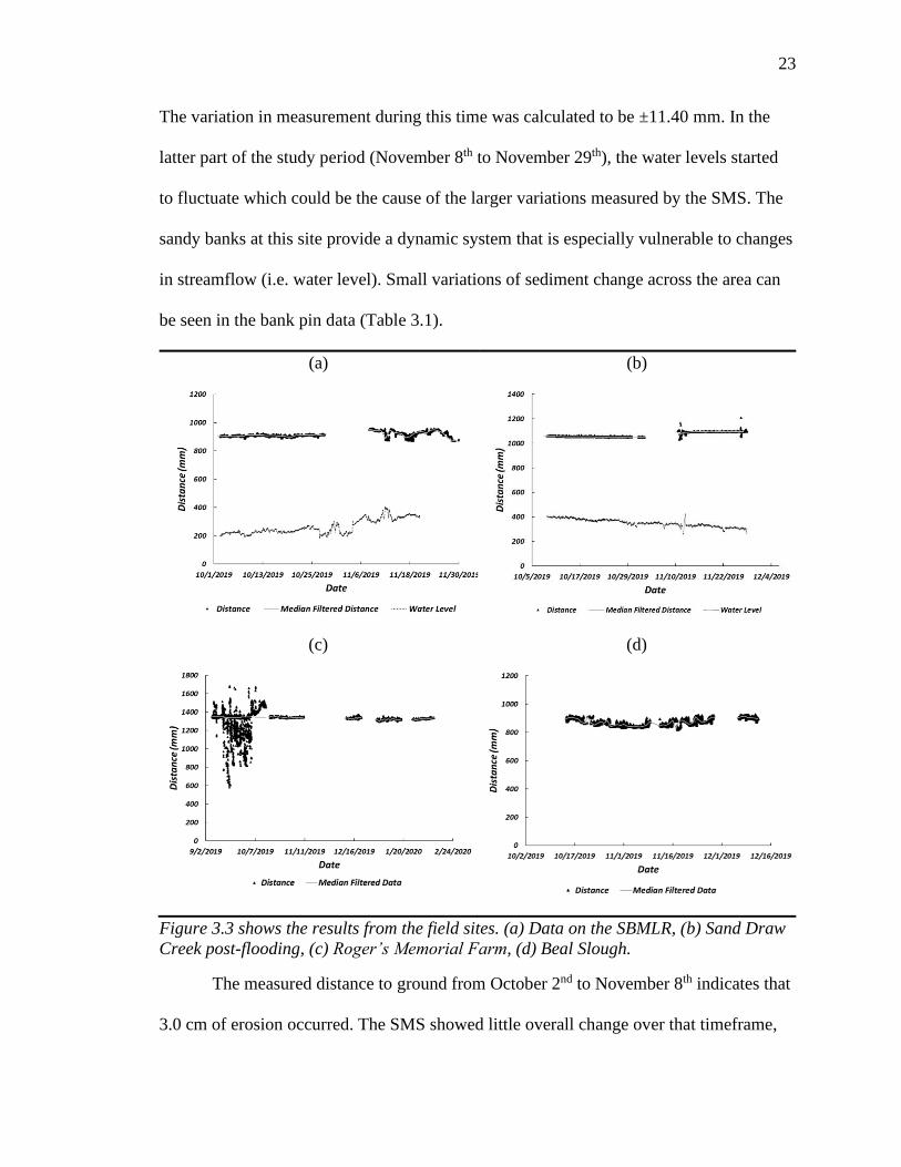
The variation in measurement during this time was calculated to be ±11.40 mm. In the

latter part of the study period (November 8th to November 29th), the water levels started

to fluctuate which could be the cause of the larger variations measured by the SMS. The

sandy banks at this site provide a dynamic system that is especially vulnerable to changes

in streamflow (i.e. water level). Small variations of sediment change across the area can

be seen in the bank pin data (Table 3.1).

(a)

(b)

(c)

(d)

Figure 3.3 shows the results from the field sites. (a) Data on the SBMLR, (b) Sand Draw

Creek post-flooding, (c) Roger’s Memorial Farm, (d) Beal Slough.

The measured distance to ground from October 2nd to November 8th indicates that

3.0 cm of erosion occurred. The SMS showed little overall change over that timeframe,

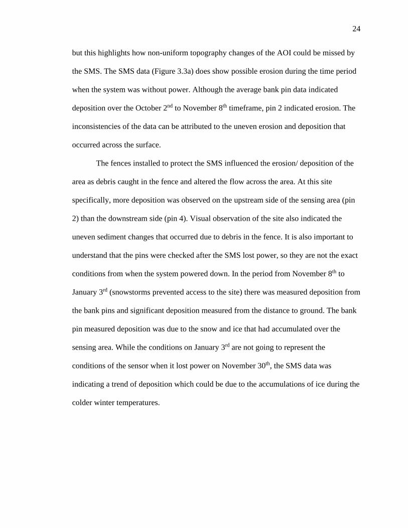
24

but this highlights how non-uniform topography changes of the AOI could be missed by

the SMS. The SMS data (Figure 3.3a) does show possible erosion during the time period

when the system was without power. Although the average bank pin data indicated

deposition over the October 2nd to November 8th timeframe, pin 2 indicated erosion. The

inconsistencies of the data can be attributed to the uneven erosion and deposition that

occurred across the surface.

The fences installed to protect the SMS influenced the erosion/ deposition of the

area as debris caught in the fence and altered the flow across the area. At this site

specifically, more deposition was observed on the upstream side of the sensing area (pin

2) than the downstream side (pin 4). Visual observation of the site also indicated the

uneven sediment changes that occurred due to debris in the fence. It is also important to

understand that the pins were checked after the SMS lost power, so they are not the exact

conditions from when the system powered down. In the period from November 8th to

January 3rd (snowstorms prevented access to the site) there was measured deposition from

the bank pins and significant deposition measured from the distance to ground. The bank

pin measured deposition was due to the snow and ice that had accumulated over the

sensing area. While the conditions on January 3rd are not going to represent the

conditions of the sensor when it lost power on November 30th, the SMS data was

indicating a trend of deposition which could be due to the accumulations of ice during the

colder winter temperatures.

25

Table 3.1 shows the results of the bank pins that were inserted just outside of the sensing

area on the SBMLR.

Date Distance to

Ground

(cm)

Pin 1

(cm)

Pin 2

(cm)

Pin 3

(cm)

Pin 4

(cm)

Average

Change

(cm)

10/2/2019

90.0 26.0 17.0 7.0 31.0 -

11/8/2019

93.0 23.7 18.3 7.0 23.5 2.1

1/3/2020 86.0 20.0 16.0 5.0 15.5 4.0

From Table 3.2 for the system at Sand Draw Creek it is clear that erosion

occurred in the sensing area. The results of the bank pins were much more consistent in

this area than the SBMLR. From October 8th to November 10th there was an average of

4.8 cm of erosion according the pins which is confirmed by the approximate change of

4.9 cm from the distance to ground measurements. The SMS data (Figure 3.3b) also

supports the erosion measured by the pins (change of 5.3 cm). While there was erosion

recorded by pins and the SMS system, the exact timing is not clear as most of the erosion

is apparent in the brief period the SMS was out of power. Slight erosion was also

measured from November 10th to December 7th by the bank pins but the distance to

ground measurement indicated little change, 0.7 cm, which is concurrent with the SMS

data (Figure 3.3b). The little change is likely due to the water level covering the sensing

area. Since water was covering most of the area, the decrease in water level could be the

cause of the “erosion” that was measured. The measured water level decrease was 3.9

cm, which is a greater reduction than was measured by pins (2.0 cm), distance to ground

(0.7 cm) or the SMS (2.2 cm). The transducer was located upstream and may have had a

larger change in water level than the bank location. The variation in measurement from

26

October 8th to November 10th was ±6.1 mm and from November 10th to November 27th it

was ±11.5 mm indicating that due to environmental factors the error was greater than the

lab results.

Lawler (1991) found similar non-changing results for a time period in their study.

The results from monitoring deposition at Sand Draw Creek confirm that no significant

sediment change occurred in the AOI during the study period. Lawler (1991) indicates

that the use of low frequency measurements cannot draw this conclusion as there is the

possibility of “complex, but balanced, sequences of sediment deposition and removal”

that can occur between measurements. Only the use of continuous timeseries data can

affirm that no significant change was measured.

Table 3.2 shows the results of the bank pins that were inserted just outside of the sensing

area at Sand Draw Creek after the system was re-installed post-flooding.

Date Distance to

Ground

(cm)

Pin 1

(cm)

Pin 2

(cm)

Pin 3

(cm)

Pin 4

(cm)

Average

Change

(cm)

10/8/2019

105.4 28.5 26.7 55.3 25.8 -

11/10/2019

110.3 41.0 27.0 55.5 30.7 -4.8

12/7/2020 109.6 44.6 29.5 55.0 33.3 -2.0

Results from the system at the Roger’s Memorial Farm are shown in Figure 3.3c.

The beginning of the monitoring period has a lot of noise and variation in the

measurement and then becomes much more consistent, only suffering gaps in the data

when the system was without power. The noise in the data is due to vegetation,

specifically corn, that started growing in the AOI. The data indicates that the corn grew to

about 52.0 cm through the month of September and was removed on October 4th. While

27

the SMS measured the growth of the corn, it also picked up the ground and had a median

value of 134.3 cm. The monitoring of the ground and vegetation are consistent with the

in-lab testing results. Even though the vegetation influenced the measurement, a

consistent measurement of the ground was also observed and showed minimal sediment

change. It was found that the system had a manufacture indicated defect in the

temperature probe during the start of the study period until it was replaced on October

14th.

After the temperature probe was replaced, the SMS did not measure a significant

sediment changing event and had a variation in measurement of ±14.9 mm. While there

was not a single sediment changing event, there was gradual sediment change from

December to mid-January where a total of approximately 2.0 cm of sediment was gained.

This could be due to environmental factors like melting snow and rainfall slowly

removing soil particles from upslope and carrying them down slope. While not designed

to pick up snow, the SMS could have measured the accumulation of snow contributing to

the variability in the measurement. Using the measuring tape, there was a change of 1.27

cm from the sensor to the ground from December 10th to January 18th, indicating that

there was some slight accumulation of sediment during this time.

Also, during the study period, the temperatures became colder and impacted the

battery life of the SMS which is especially apparent in the timeseries data from the

Roger’s Farm. There were frequent gaps in the data because the battery life was reduced

due to the colder temperatures. Typically, the battery life was approximately 28 days, but

the cold temperatures reduced the battery life to approximately 12 days. Cold

28

temperatures caused the SMS, at all sites, to have reduced battery life and to become

inactive until new batteries were installed.

Figure 3.3d shows the timeseries data from the erosion monitoring SMS at Beal

Slough. This time series has a larger variation in the data visually. While there were no

bank pins used at this site, visual inspection of the bank during checks indicated that no

significant erosion occurred. Water levels were always significantly lower than the AOI

which was located near the top of the cut bank and should not have impacted the AOI.

The variation in measurement was ±52.4 mm, which is significantly higher than errors

from other sites. More error may be present in this site for a couple reasons. The longer

cable the SMS used to monitor erosion could be picking up external noise and impacting

the signal. It is also possible that there is more audio noise present in this urban location

that is impacting the ultrasonic sensor. Finally, a culmination of environmental factors

compounding on one another is likely another reason more error is seen in this

measurement, as environmental factors caused greater error at other sites. Each factor has

small impacts that amounted to a large error range.

Results from the field studies revealed greater error in measurement than

compared to the lab results. This is likely due to environmental impacts. While the SMS

has many applications and benefits from traditional monitoring methods, it is limited by

its accuracy in measurement from environmental factors. The most influential factor

affecting the speed of sound is the air temperature. Changes in air temperature can cause

the speed of sound to change. As temperatures get warmer, speed of sound increases and

as temperatures get cooler the speed of sound decreases (Bohn, 1988). This can cause

measurement error with the ultrasonic sensor as the temperature changes throughout the

29

day and was why a temperature probe was included in the SMS to correct for temperature

effects on the speed of sound. While temperature was corrected for, there could still be

slight error in measurement from temperature as the temperature profile changes from the

ground upward. The proximity to flowing water could also impact the temperature and

relative humidity of the air.

Another important environmental factor that can affect the speed of sound is the

moisture content of the air or the relative humidity. Relative humidity is dependent on air

temperature as warm air is able to hold more moisture than cooler air. The relative

humidity impacts the speed of sound because sound waves travel through the air medium

and as the medium changes, sound wave propagation will change. When at a temperature

of 20 Celsius, the speed of sound can change by approximately 1 meter per second when

the relative humidity changes from 0% to 100%, increasing in speed as the relative

humidity increases (Chen & Maher, 2004). Coupling in the effects of temperature and

relative humidity, in general the speed of sound travels even faster in warm, moist air.

This means that even when accounting for temperature, the speed of sound is still

changing as the relative humidity changes with temperature. Thus, correcting for the

relative humidity would allow for even more precise measurements.

Wind impacts sound by changing the speed of sound depending on which

direction the sound waves is traveling with respect to the wind direction. The sound wave

is a mechanical wave traveling through a moving medium (air), so as the speed of the

medium changes the speed of sound changes. The speed of sound is relative to that of the

medium; meaning relative sound velocity is the sum of the sound velocity and wind

velocity. The wind, along with temperature, can also cause the refraction of sound waves,

30

though this tends to happen over large distances and should be negligible within distances

covered in this study (Ingard, 1953 and Chen & Maher, 2004).

While there are limitations of the SMS with respect to environmental factors,

variations in measurement could also have been impacted by the slight sediment changes.

Lawler (1991) found that even in periods of suspected inactivity, minimal water level

fluctuations, there was frequent, small-scale changes in sediment recorded by the PEEPs.

The SMS found similar small-scale changes during varying time periods at all the sites.

While there was no suspected activity to cause sediment changes, wind erosion and

splash erosion could play significant roles of contributing to these small-scale sediment

changes. The dynamics of sediment change account for the fluctuations seen in

measurements during periods of suspected inactivity, like at the Roger’s Memorial Farm

and Beal Slough. These small-scale changes could have contributed to having increased

error in measurements.

While the SMS is affected by environmental factors, the error in measurement is

comparable and even better than some sediment monitoring methods. We found an error

in measurement of ±6.1 - 52.4 mm for the SMS in the field (±1.0 – 8.0 mm for the lab).

The low end of our interval, and in lab testing, is comparable to Lawler’s (2001)

resolution of ±2 - 4 mm, but not as good as Plenner’s (2016) TLS error of 0.36 mm

between actual and measured results. While not as good as some other methods, the SMS

was significantly better than Cook’s (2017) UAV imagery analysis error of 30 - 45 cm.

While the SMS may not provide the highest resolution results, it does have

advantages over other current monitoring methods. The SMS is able to continuously

monitor an AOI, day or night, for extended periods of time unlike Lawler’s PEEPs that

31

only work during daytime and Plenner’s TLS which is only set up for short periods of

time and only during low flow events. The SMS is designed to have water levels rise

above the sensing area so it can capture the exact sediment altering events. This ability is

showcased in Figure 3.4, which depicts data from Sand Draw Creek during the flooding

stages of the stream. While the data recorded was not on the most up-to-date SMS, defect

temperature probe and average filter instead of median filter, the SMS was still able to

accurately measure the exact timing of the water level rise and subsequent deposition as

water levels dropped. The first water level peak occurred on August 12th as measured by

the pressure transducer. The water level rise was also measured by the SMS as it rose

above the sensing area. As the water level decreased, sediment was deposited as

measured by the SMS to be 24.8 cm. There was another water level peak measured by the

pressure transducers on September 2nd and also measured by the SMS. When the water

level dropped 18.7 cm of deposition was recorded by the SMS. The flood waters altered

the SMS set up and eventually debris build up caused the mounting posts to bend and

flood the system. While the SMS was ruined, the data was able to be removed from the

SD card. The bank pins that were inserted during this time were unable to be located after

the significant sediment build up.

32

Figure 3.4 highlights the SMS ability to capture timing of deposition causing events. Two

large rainfall events at the Sand Draw Creek site caused major water level rise, flooding

and sediment deposition.

The results demonstrate two things, first the SMS has the capability of measuring

the timing of erosion and deposition events and second can provide accurate

measurements (within 5 cm) of sediment change in the AOI. While the SMS can provide

sediment change data with a resolution within 5 cm, the accuracy could be improved by

combining the SMS with another traditional monitoring method to get finer

measurements. Using a traditional monitoring method would also be necessary to obtain

sediment change information across a larger area. While the SMS monitors an area of

2,826 cm2, it does not currently provide information of an entire bank like the TLS, aerial

imagery or gridded bank bins. Combining the SMS with another affordable method, like

33

gridded bank pins, would allow for precise measurements of an entire bank while also

providing the timing of when sediment changes occur.

Though limited in measurement resolution for small sediment changes, locations

that undergo large sediment changing events can be monitored by the SMS with little

issues in recording the quantity of sediment. The high flow events at Sand Draw Creek

highlight the SMS capability. The SMS recorded a total deposition amount of 43.5 cm

with an error of ±10.79 mm. Comparing this result to Midgley et al. (2012)’s study,

where approximately 7.9 to 20.9 m of bank laterally eroded on a Barren Fork Creek in

northeastern Oklahoma. They used BSTEM to model the failure events, but the model

under predicted the quantity of erosion by a couple meters, though accurately predicted

the timing of the erosion events. The SMS was able to provide more accurate results

during the high flow events of this study. This shows that the SMS can accurately

monitor large sediment changing events, capturing both the timing and quantity.

34

CHAPTER 4: RESILIENCE, POLICY AND OUTREACH IN RIPARIAN

ECOSYSTEMS

One possible application of the SMS would be for the monitoring of alternative

state thresholds. In rangeland or riparian ecosystems there are two contrasting states that

can occur, vegetated and bare/ sparsely vegetated states which influence erosion

processes (Chartier & Rostagno, 2006). In resilience theory, alternative stable states refer

to the potential alternative configuration of functions, processes and abundance and

composition of a system (Angeler & Allen, 2016). For a regime shift to occur, a threshold

must be surpassed. The threshold can be described as a tipping point in which the ball

resides in a different basin of attraction (Gunderson, 2000). Chartier et al. (2006) defines

a site conservation threshold as the point at which the rate of soil erosion increases

markedly. This spike in erosion rate is due to the reduction in vegetation and marks the

transition into an alternative state from vegetated to sparsely vegetated. The change in

state can also move the other way. A sparsely vegetated, significant erosion prone area

can recover into a vegetated, reduced erosion prone area if the perturbation, loss of

vegetation, is reduced or halted (Kauffman, Case, Lytjen, Otting, & Cummings, 1995). A

long-term, continuous monitoring erosion device like the SMS is required to measure

when a threshold is surpassed, and the system moves into a new state.

In order to identify the site conservation threshold when the erosion rate increases

significantly, a monitoring device is needed that is able to record data at a high frequency

so the erosion rate can be measured and the timing of the regime change can be

monitored. It is also important that the device be non-invasive so as not to alter the

structure of the area and influence erosion rates. Both of these aspects are accounted for

35

in the SMS. Erosion is a natural process that occurs in all systems at varying degrees of

severity. The management of erosion should not focus on stopping the process, but on

managing areas to reduce the erosion rate, supporting systems to withstand perturbations

and monitoring the eroding areas to track erosion rates and identify when a regime shift

occurs. Understanding the regime changes in riparian areas can help improve the

resilience, the ability of a system to maintain structure, function, and relationships while

experiencing (perturbations) pressure to change (Holling, 1973), of the streambank to

withstand greater perturbations before experiencing a regime shift. It will also allow

managers insight into how to restore a riparian area into a more desirable state, usually a

vegetated state with reduced erosion.

One way managers can help reduce erosion and maintain desired states is to use

riparian buffers. Riparian buffers are undeveloped strips of land that flank water ways.

Using riparian buffers reduces the effects of vegetation loss due to farming, grazing, or

urban development. The buffers should be planted over with native grasses, shrubbery, or

trees to help with the filtration of nutrients from runoff and to help stabilize soil and

reduce erosion. While there are many benefits of riparian buffers such as water quality

improvements, reduction in erosion and habitat for wildlife and shading for aquatic life

(Burden, 2015); it also takes away from the amount of land that is available to develop,

whether that is for agriculture or industry.

There are agencies at multiple levels that work to manage riparian areas through

the use of riparian buffers. Examples include the USDA-NRCS at the federal level and

different state level departments, like Nebraska’s Department of Natural Resources

(NeDNR). There are also local agencies like Nebraska’s Natural Resource Districts

36

(NRDs) which focus on smaller regional management of water resources. Other

organizations work to support streambank restorations and riparian buffers like The

Nature Conservancy and Pheasants Forever. While there are many management agencies,

without policies requiring riparian buffers, implementation is strictly voluntary. Solutions

for effective soil sustainability, like riparian buffers, will require interdisciplinary

communication between policy makers, public institutions, and natural resource

managers (Amundson, et al., 2015). An example of utilizing policy makers to take action

can be seen in Minnesota with their 2017 policy mandating all waterways have a 50ft

buffer and all drainage ditches have buffers of 16.5 ft (MN Stat. § 103F.48). This policy

includes provisions for the local water resource management agency to work with

landowners on implementing these buffers. As of July 2019, there was a 98% compliance

rate with the law. This compliance includes lands that are in planning stages riparian

buffer development. In order to achieve high compliance with this law, engagement and

outreach techniques were likely used to encourage landowners to make the needed

changes in a timely manner.

Outreach and engagement can be a powerful tool for implementing best

management practices for the improvement of natural resources. Riparian buffers can be

considered a best management practice (BMP) that any landowner can implement along

waterways. Proper engagement and outreach require the involvement of the landowners

during the planning process. This means informing the landowners, providing channels

for their ideas and concerns to be voiced and most importantly addressing the ideas and

concerns (Twyford, Waters, Hardy, & Dengate, 2006). Communicating with landowners

in the process of implementation of riparian buffers or any other BMP will help build

37

trust and assist with reaching compliance of implementation. Busse et al. (2015) found

that outreach is not always effective in getting the desired message out to as wide of an

audience as desired, however individuals that did receive the message showed positive

changes in their attitude.

Beyond effective communication with landowners, understanding the

demographic and challenges faced by landowners from the expected change are essential

in having a successful adoption of new policies. Busse et al. (2015) also found that the

best way to ensure successful outreach efforts is to understand the public perceptions on

topics related to solution implementation as well as determining what type of outreach

would be most effective for the demographic. This means that it is important to tailor

outreach and engagement efforts to each situation and not try a blanket approach.

Understanding the demographic being engaged ensures the correct messaging can

be deployed to the correct audience. For example, there are multiple levels of

comprehension and perceived responsibility between agricultural and non-agricultural

residents regarding water quality and nutrient pollution (Busse, et al., 2015). Each group

requires different outreach processes to help them better understand water quality and

nutrient pollution. It is also important to understand how the demographic perceive and

trust outreach personnel. Hoorman and Spencer (2002) highlight the need for trust in a

community during outreach through their work with Amish communities. The authors

show that the best way to engage these particular communities is to bring outreach

activities directly to their homes and businesses in order to build trust within the

community. Many landowners and agricultural producers tend to trust and receive

messages better from University Extension, Soil and Water Conservation Districts, and

38

Natural Resource Conservation Service personnel (Mase, Babin, Prokopy, & Genskow,

2015). Building trust in communities when conducting outreach is vital for the success of

the outreach and engagement programs. The implementation of policies can quickly be

applied through outreach and engagement processes, so the best management of natural

resources can be conducted across broad areas.

39

CHAPTER 5: CONCLUSTIONS AND FUTURE WORK

Lab testing demonstrated that the SMS has a measurement error of approximately

±1.06 mm when measuring at a distance of 1.25 meters and increases slightly as the

distance increases. Field testing revealed that there are environmental factors that

influence the SMS measurements. While temperature is being corrected for, wind and

relative humidity could still be impacting the measurement. The measurement error for

the field sites ranged from ± 6.12 to 52.42 mm, with the latter error likely being

influenced by urban noise, signal noise from an extended cable and other environmental

factors. The SMS was used to accurately measure the timing and quantity of two

deposition causing events after high flows were observed on Sand Draw Creek. While the

magnitude of these deposition events were unable to be confirmed with erosion pin data,

due to loss of pins, the previous testing has indicated that the total measured 43.5 cm of

sediment deposited between the two high flow events is within approximately 10.79 mm

(average error of three measured errors, excluding extraneous error value 52.42 mm) of

the actual amount. Coupling the SMS with another erosion monitoring method would

allow for more precise measurements to be taken on sediment change amounts while still

being able to understand the timing of sediment changing events.

Future work will focus on correcting for other environmental factors, such as

relative humidity and wind, that can affect the sensing capability of the SMS. Increasing

the battery life of the SMS is also important for the continuation of long-term erosion and

deposition studies. Ideally extending the battery life to 3 months and incorporating a solar

panel would reduce the time spent in the field and the gaps in data. Finally, incorporating

40

telemetry technology to transmit data from the SMS directly to users would decrease

field time and ensure data is captured and not lost if high flows were to destroy the SMS.

The SMS has the capability of measuring sediment change continuously and non-

invasively for extended periods of time. Since there is a need for a greater understanding

of gully erosion, the SMS would be ideal for monitoring gullies as they get deeper and

wider due to erosion. This data could then be used to help develop better models for

predicting gully erosion or for better quantifying the amount of gully erosion occurring in

landscapes and helping to improve the management of erosion prone areas. Using

interdisciplinary approaches, major challenges of managing erosion and deposition can

be addressed and solutions formed.

41

REFERENCES

Amundson, R., Berhe, A. A., Hopmans, J. W., Olson, C., Sztein, E. A., & Sparks, D. L.

(2015). Soil and human security in the 21st century. Science, 384(6235).

Angeler, D. G., & Allen, C. R. (2016). Quantifying resilience. Journal of Applied

Ecology, 53(3), 617-624. doi:doi.org/10.1111/1365-2664.12649

Bernhardt, E. S. (2005). Synthesizing U.S. river restoration efforts. Science, 308(5722),

636-637.

Bohn, D. (1988). Environmental Effects on the Speed of Sound. Journal of Audio

Engineering Society, 36(4).

Borrelli, P., Robinson, D., Fleischer, L., Lugato, E., Ballabio, C., Alewell, C., . . .

Panagos, P. (2017). An assessment of the global impact of 21st century land use

change on soil erosion. Nature Communications, 8(2013), 1-13.

Burden, D. (2015). Small Farm Sustainability: What is a Riparian Buffer? Ames, IA:

Iowa State University Extension and Outreach.

Busse, R., Ulrich-Schad, J. D., Crighton, L., Peel, S., Gensknow, K., & Prokopy, L. S.

(2015). Using Social Indicatiors to Evaluate the Effectivness of Outreach in Two

Indiana Watersheds. Journal of Contemporary Water Research and Education,

156, 5-20.

Carey, B. (2006). Gully Erosion. Queensland Government Department of Natural

Resources and Water, L81, 1-4.

Chartier, M. P., & Rostagno, C. M. (2006). Soil Erosion Thresholds and Alternative

States in Northeastern Patagonian Rangelands. Rangeland Ecology and

Management, 59(6), 616-624.

Chen, Z., & Maher, R. (2004). Atmospheric Sound Propagation Considerations for the

Birdstrike Project. Montana State University.

Cook, K. (2017). An evaluation of the effectiveness of low-cost UAVs and structure from

motion for geomorphic change detection. Geomorphology, 278, 195-208.

Department of Environment and Resource Management, Q. G. (2011). Wind Erosion.

State of the Environment Fact Sheet L259, 1-2.

FAO. (1978). Soil Erosion by water. Agricultural Development Paper No. 81 2nd

printing, 284.

FAO. (1978). Soil erosion by wind. Agricultural Development Paper No. 71. 4th

printing, 88.

Gunderson, L. H. (2000). Ecological Resilience--In Theory and Application. Annual

Review of Ecology and Systematics, 31, 425-439.

42

Holling, C. S. (1973). Resilience an Stability of Ecological Systems. Annual Review of

Ecology and Systematics, 4(1), 1-23.

Hoorman, J. J., & Spencer, E. A. (2002). Engagement and Outreach with Amish

Audiences. Journal of Higher Education and Engagement, 7, 157-168.

Ingard, U. (1953). A Review of the Influence of Meteorological Conditions on Sound

Propagation. Journal of the Acoustical Society of America, 25(3), 405-411.

Kauffman, J. B., Case, R. L., Lytjen, D., Otting, N., & Cummings, D. L. (1995).

Ecological Approaches to Riparian Restoration in Northeast Oregon. Pacific

Northwest Reports: Restoration and Management Notes, 13, 12-15.

Klavon, K., Fox, G., Guertault, L., Langendoen, E., Enlow, H., Miller, R., & Khanal, A.

(2017). Evaluating a process-based model for use in streambank stabilization:

insights on the Bank Stability and Toe Erosion Model (BSTEM). Earth Surfaces

Processes and Landforms, 42, 191-213.

Lague, D., Brodu, N., & Leroux, J. (2013). Accurate 3D comparison of complex

topography with terrestrial laser scanner: Application to the Rangitikei canyon

(N-Z). ISPRS Journal of Photogrammetry and Remote Sensing, 82, 10-26.

Lal, R. (1994). Soil Erosion by Wind and Water: Problems and Prospects. In R. Lal, Soil

Erosion Research Methods Second Edition (2nd ed., pp. 1-7). Delray Beach,

Florida: St. Lucie Press.

Lawler, D. (1991). A New Technique for the Automatic Monitoring of Erosion and

Deposition Rates.

Lawler, D. M. (1993). The measurement of river bank erosion and lateral channel

change: A review. Earth Surface Processes and Landforms, 18, 777-821.

doi:doi:10.1002/esp.3290180905

Lawler, D. M. (2001). The Photo-Electronic Erosion Pin (PEEP) Automatic Erosion

Monitoring System: Principles and Application. 7th Federal Interagency

Sedimentation Conference, 1, 56-59.

Mase, A. S., Babin, N. L., Prokopy, L. S., & Genskow, K. D. (2015). Trust in Sources of

Soil and Water Quality Information: Implications for Environmental Outreach

and Education. Journal of the American Water Resources Association, 51(6),

1656-1666.

Maxbotix. (2012). HRXL-MaxSonar ®-WR ™ Series. MaxBotix Inc., Baxter, MN.

Maxbotix. (n.d.). Temperature Compensation Report. MaxBotix Inc., Baxter, MN.

Midgley, T. L., Fox, G. A., & Heeren, D. M. (2012). Evaluation of the bank stability and

toe erosion model (BSTEM) for predicting lateral retreat on composite

streambanks. Geomorphology, 107-114.

43

Nebraska-Lincoln, U. o. (2020). Roger's Memorial Farm. Retrieved from Biological

Systems Engineering Department: https://engineering.unl.edu/bse/bse-rogers-

memorial-farm/

NIST. (n.d.). What are outliers in the data? Retrieved from Engineering Statistics

Handbook: https://www.itl.nist.gov/div898/handbook/prc/section1/ prc16.htm

Pimentel, D., Harvey, C., Resosudarmo, P., Sinclair, K., Kurz, D., McNair, M., . . . Blair,

R. (1995). Environmental and economic costs of soil erosion and conservation

benefits. Science, 267(5201), 1117-1123.

Plenner, S., Eichinger, W. E., & Bettis, E. A. (2016). Simple Terrestrial Laser Scanner

for Measuring Streambank Retreat. Journal of Hydrualic Engineering. doi:DOI:

10.1061/(ASCE)HY.1943-7900.0001184

Poesen, J. (2011). Challenges in gully erosion research. Landform Analysis, 17, 5-9.

Poesen, J. (2017). State of Science Soil erosion in the Anthropocene: Research needs.

Earth Surface Processes and Landforms, 43, 64-84.

Poesen, J., Nachtergaele, J., Verstraeten, G., & Valentin, C. (2003). Gully erosion and

environmental change: importance and research needs. Catena, 50, 91-133.

Riparian Protection and Water Quality Practices. (n.d.). MN Stat.: 103F.48.

Schwab, G. O., Fangmeier, D. D., & Elliot, W. J. (1996). Soil and Water Management

Systems. John Wiley and Sons, Inc.

Thorne, C. (1981). Erosion and Sediment Transport Measurement. IAHS Publ.

Trunk, T., Miller, M., & Pica, J. A. (2018). Requirements and Standards for NWS

Climate Observations. National Weather Service Instruction 10-1302, pp. 7-8.

Twyford, V., Waters, S., Hardy, M., & Dengate, J. (2006). Beyond Public Meetings:

Connecting Community Engagement with Decision Making. Vivien Twyford

Communication.

44

APPENDIX A: USER GUIDE

This guide covers the construction and installation of the Sediment Monitoring System.

Construction:

1. Gather electronics components, the following is a list of components used:

a. Arduino Nano ~ $22.00

b. Gikfun SD Storage Board TF Card Memory Shield Module for Arduino

(Arduino Shield) ~ $8.00

c. Adafruit DS3231 Precision RTC Breakout Board (RTC) ~ $14.00

d. SanDisk microSD Card and Memory Card Adapter ~ $12.00

e. MaxTemp Temperature Probe ~ $10.00

f. MaxBotix Ultrasonic Sensor (MB7389 HRXL-MaxSonar-WRMT) with

shielded cable ~ $173.00

g. Mighty Max 22 amp-hr 12V deep cycle battery ~ $45.00

2. Connect the Arduino Nano to the Arduino Shield to make wiring easier. Wire

Arduino Nano/ Shield, RTC and SD card adapter components according to the

wiring guide found in Appendix B. Some components may require soldering to

secure wires or wiring pins.

3. Drill holes in housing box for the ultrasonic sensor wire and temperature probe

wires to run through. Using water resistant gromets run ultrasonic sensor wire and

temperature probe wires through holes.

(Note: Before running ultrasonic sensor wire through the gromet and hole,

ensure the mounting hardware has been attached to the ultrasonic sensor.

This was a metal plate with holes for U-Bolts and a hole allowing the

cable and back end of the sensor through. A pipe fitting was screwed onto

the sensor’s back end to secure the sensor in place.)

4. Secure the electronics components and mount in weather resistant box.

Electronics were mounted to plexiglass, using electronics screws and spacers,

which was screwed into housing box.

5. Wire the ultrasonic sensor and temperature probe into Arduino system according

to Appendix B. The temperature probe is wired to the temperature compensation

wire on the ultrasonic sensor (Pin 1, white wire) and then to ground.

45

6. Attach mounting brackets to housing box. These were machined metal brackets to

allow U-Bolts to fit through and secure to T-Posts.

Installations:

1. Upload code to the Arduino Nano (consult Appendix C: Code). Ensure code

matches sensor range and proper measurement frequency is set.

(Note: When uploading code, the sensor wires (blue and green) need to be

detached from the RX and TX inputs to the Arduino Nano.)

2. Determine the area-of-interest (AOI) for observing. This should be an area

experiencing erosion or likely to have deposition occur. Make sure the location

will allow for secure placement of the SMS.

(Note: If installing near a stream, confirm that the housing box can be

mounted at an elevation above high water marks. This can be done by

mounting it near the top of the T-Post.)

3. Installation and ultrasonic mounting styles will vary based on what is to be

observed and on limits from each site. Ensure that the ultrasonic sensor is facing

perpendicular to the AOI (See figure A.1 below).

(Note: If using T-Posts to mount the SMS and using a horizontal mounting

arm with a T-Post bracket, ensure the “T” of the T-Post is facing towards

the AOI. Also, make sure the horizontal mounting arm is braced to prevent

it from swaying and bouncing in the wind.)

4. Insert SD card into SD card adapter. Make sure there is a click denoting that the

SD card was fully inserted into the adapter.

5. Connect the battery to the system and start collecting data. To ensure the system

is recording the AOI, refer to the lights on the Arduino to determine if a

measurement has been taken. The TX light should always be on, when the SMS is

taking a reading the RX light will flash. Once the reading is taken the RX light will

blink solid as it saves to the SD card and then turn off until the next reading.

(Note: To force the system to record a measurement, press the reset button

on the Arduino, white rectangle in the middle of the board adjacent to the

system lights. This triggers the SMS to take a measurement and reset the

measurement frequency timer.)

46

Maintenance:

1. Charge and replace batteries as needed. (Approximately 28 days with MightyMax

12V-22amp-hr battery)

2. When downloading data from SD card, cut power to the SMS, eject the SD card

and download onto computer. Delete data from SD card but keep the TEST.txt

file to ensure the system recognizes a file to store data to. Replace SD card and re-

connect power to continue monitoring.

3. Check and update that the date and time is accurate during measurements.

Sometimes the RTC is reset when the system is without power for extended

periods of time.

4. Always keep the ultrasonic sensor mounted in the same position while moitoring

an area. Changing the position will influence the distance reading and will give

inaccurate values of erosion or deposition when compared to the previous

position.

5. Ocasionally check the cone of the ultrasonic sensor to ensure no obstructions have

lodged themselves in the cone and blocked the sensor’s view.

Streambank Erosion Deposition/ Field Erosion

(a)

(b)

Figure A.1 shows two different mounting techniques used for different SMS installations.

47

APPENDIX B: WIRING GUIDE

Included is the wiring diagram which shows how to connect the ultrasonic sensor,

RTC and SD card module to the Arduino Nano. The pins connections shown here reflect

the pin connections as defined in the code used for operation.

48

49

APPENDIX C: CODE

Full scripts of the code used to control the SMS can be downloaded at

https://github.com/jejohnson14/Sediment-Monitoring-System. Below are a couple lines

of code showing how to change the frequency in measurement for the SMS.

The code is in total 213 lines and should be run using the Arduino code interface

for ease of editing and uploading to the Arduino Nano microcontroller. Depending on the

range of the ultrasonic sensor used, there are two scripts available on GitHub:

MedianReading10M.ino and MedianReading5M.ino. They are the same script except the

limiting distance for which an error in reading is thrown is changed to the corresponding

range limit. Also included are scripts to help set the RTC clock and test the SD card

module connection.