Monthly Time-Step Erosion Risk Monitoring of Ishmi-ErzeniWatershed, Albania, Using the G2 Model

Christos G. Karydas1 & Pandi Zdruli2 & Spartak Koci2 & Fatbardh Sallaku3

Received: 26 April 2013 /Accepted: 18 March 2015# Springer International Publishing Switzerland 2015

Abstract In this study, soil erosion was mapped in Ishmi-Erzeni watershed, Albania, using the G2 model. The G2 mod-el has been proposed as an agri-environmental service by theGlobal Monitoring for Environment and Security (GMES)initiative (now Copernicus programme). Based on the princi-ples of the Universal Soil Loss Equation (USLE), G2 providesmaps of actual soil loss at a monthly time-step. The maininnovations of the model with regard to previous USLE fam-ily models are as follows: the introduction of a ‘storm factor’,which differentiates rainfall erosivity (R factor) per monthwhen detailed rain intensity records are not available; theuse of standardised biophysical parameters derived from sat-ellite image time series in combination with land use informa-tion for calculating the vegetation retention factor (denotedhere as V factor, corresponding to C factor of USLE); andthe use of satellite imagery for calculating a new factor, name-ly the slope intercept factor (denoted as I factor), which ex-presses landscape feature alterations, thus functioning as cor-rective to the topographic influence factor (denoted here as Tfactor, the slope length and steepness (LS) factor of USLE).

The model was originally implemented in the cross-borderStrymonas river basin and on the island of Crete after revision;in both cases with encouraging results. The G2 model followsa data-driven methodology, while providing alternatives forall factor estimations with moderate data requirements. Forthe model application in the Ishmi-Erzeni watershed (covering2200 km2), rainfall data were collected from ten weather sta-tions, and soil properties were measured from sampling at 47locations. Vegetation layers were downloaded from theGMES portal, while land use information was extracted froma Landsat-7 TM image. Finally, terrain properties were calcu-lated from a 250-m digital elevation model (DEM) of the area.The G2 model showed Ishmi-Erzeni to have moderate soilerosion, with a mean annual soil loss estimated to be 6.5 t/ha; however, 18 % of the area is facing an annual risk of soilremoval more than 10 t/ha, which is considered to be a sus-tainable threshold for Albania.Winter months appear to be themost risky, with all months contributing substantially to theannual erosion rate (i.e. between 4 and 12 % each). Areas ofconiferous and mixed forests, together with mountainous ag-ricultural land, appear to be the most risky land uses. In con-clusion, the G2 model proved to be useful and efficient forpredicting erosion at monthly time-steps for all land uses inthe Ishmi-Erzeni watershed. Future research will focus on anAlbania-wide erosion mapping task, using the G2 model.

Keywords USLE . Gavrilovic . Storm factor . Vegetationretention . Biophysical parameters . Slope intercept

1 Introduction

Soil erosion is the process of detachment and transport of soilmaterial by wind or water [12] and is considered to be anenvironmental threat with on-site and off-site impacts [9].

* Christos G. Karydasxkarydas@auth.gr

1 School of Agriculture, Forestry and Natural Environment, Lab ofForest Management and Remote Sensing, Aristotle University ofThessaloniki, University campus, 54124 Thessaloniki, Greece

2 Mediterranean Agronomic Institute of Bari Land and WaterResources Management Department, International Centre forAdvanced Mediterranean Agronomic Studies (CIHEAM), ViaCeglie 9, 70010 Valenzano, Bari, Italy

3 Faculty of Agriculture and Environment, Department ofAgroEnvironmental and Ecology, Agricultural University of Tirana,Tirana, Albania

Environ Model AssessDOI 10.1007/s10666-015-9455-5

According to the Global Assessment of Human-Induced SoilDegradation (GLASOD) [27], 17 % of the vegetated land onEarth is considered to be degraded largely by erosion, and 1out of 6 ha of this land could be considered no longer suitablefor cultivation. Taking into account the effect of the climatechange in a global context, which is expected to increase ratesand impacts of soil erosion, Yang et al. [41] have estimatedthat a thickness of 0.38 mm of soil is likely to be lost on anannual basis. Deforestation and adverse farming practices,such as overgrazing, have been determined as the main causesof this environmental disaster [36]. Soil erosion has been iden-tified as an urgent environmental threat in Europe by the SoilThematic Strategy of the European Union ([44] 46 final).

Soil erosion is widely discussed in the literature on desert-ification [4, 3] and is believed to be one of the most degradingprocesses affecting land resources. According to the UNCCDdefinition, desertification is defined as land degradation inarid, semi-arid and dry subhumid areas resulting from variousfactors, including climatic variations and human activities(WMO [47]; UNCCDs [48]).

Albania is particularly vulnerable to soil erosion,experiencing long and heavy rainfall events in all seasons(especially autumn and winter) and consisting of steep terrain.Further accelerated by inappropriate land management [14],erosion is estimated to affect 24 % of the Albanian territory,with average annual soil losses of 37 t/ha [42]. Studies usingwatershed sediment assessment methods indicate that the rivernetwork transports more than 60 million tons of sedimentsevery year [21]. The hydrographical network of Albania isvery dense with rivers and streams draining into the Adriaticand Ionian Seas.

Soil erosion is the result of several interacting processes inspace and time; therefore, measuring or estimating soil loss byerosion is a difficult undertaking [9]. Since the 1930s, soilscientists and decision makers have been developing and test-ing models extensively to calculate soil loss from field plots,hill slopes or small watersheds [40]. With the rise and signif-icant improvements in Geographic Information Systems(GIS) together with the advances made in computing power,efforts have concentrated on spatially distributed models,which simulate the runoff and erosion dynamics of largerand more complex catchments [17]. Introduction of spatialrelationships in model structures has increased modelling un-certainty. For a recent review and complete inventory of watererosion models, see Karydas et al. [18].

With a view to serve as an agro-environmental tool, a newerosion model was developed in the framework of the GlobalMonitoring for Environment and Security (GMES) initiative;GMES has been now renamed into ‘Copernicus programme’(http://www.copernicus.eu). This model, namely the G2model, is an output of the ‘geoland2’ project and specificallyof the AgriEnv action. G2 is a data-oriented model, inheritingthe experience gained form the Universal Soil Loss Equation

(USLE) and the Erosion Potential Method (EPM; also knownas ‘Gavrilovic’), and being able to provide soil loss maps on amonth-step under present or potential vegetation cover, landuse and climatic conditions. The model was first implementedand tested in the Strymonas (or Struma) river basin, a 14500-km2 cross-border study area, shared mainly between Greeceand Bulgaria, on a regional scale (1:500,000) [28].

A revised version of G2was then applied in Crete (Greece),an island covering 8336 km2. The revision of the model fo-cused on the introduction of a new parameter reflecting theinfluence of land use on soil loss processes based on empiricaldata fromUSLE and EPM (Gavrilovic) erosionmodels; all theoriginal formulas were reset accordingly [31]. Efforts are cur-rently underway to implement the G2model in a country-wideassessment (application in Cyprus is underway and scheduledfor Greece). The G2 model has been made available to deci-sion makers and researchers as an item in the Soil ErosionTheme of the European Soil Data Centre (ESDAC) of theJoint Research Centre [29], through provision of guidance,data sets and support to potential users (http://eusoils.jrc.ec.europa.eu/library/themes/erosion/G2/data.html).

The aim of this research was to map actual soil loss in theIshmi-Erzeni watershed, Albania, with a view to detect criticalsites, seasons and land uses in the area. The basic hypothesiswas that the use of the G2 erosion model would be necessaryand efficient to provide information required for supportingland use management and indicate appropriate mitigationmeasures in this area. An extra objective was the productionof harmonised and comparable maps and statistics as a base-line for future assessments in the Ishmi-Erzeni study area andfor Albania in general.

2 Materials and Methods

2.1 Study Area

Albania is located in the southwestern part of the Balkan Pen-insula with most of the country covered by hills and moun-tains and a mean altitude of 708 m. The Ishmi-Erzeni water-shed is one of the most populated places in Albania compris-ing extensive agricultural and forested lands. The area hassuffered extreme urbanisation of the flat areas, especiallythose surrounding the capital of the country Tirana and thecity of Durres, and the ravages of gravel extraction on theErzeni and Ishmi river beds to support the constructionindustry.

The Ishmi-Erzeni watershed comprises a complex of tworiver basins (River Ishmi and River Erzeni) and some smallcoastal watersheds, located in the central-western part of Al-bania. Its main orientation is east-west, covering a total area of2200 km2. River Erzeni is the longest river of the basin (about109 km), rising in the eastern Tirana mountains, close to

C.G. Karydas et al.

Shengjergj village and flowing to the Adriatic Sea, northern ofDurres [35]. The two rivers flow at only a small distance apart(about 7 km) when they cross Tirana area. The Ishmi-Erzenicomplex can be divided into three agro-ecological zones: themost productive agricultural lowlands along the Adriaticcoast, the hilly areas cultivated with fruit trees, olives andgrapes or covered by scrubs and the mountainous zone withsome crops in the valleys and forestry or livestock pasture inthe highlands, where overgrazing is a common practice [22](Fig. 1).

The area is characterised by moderately hot summers withstrong solar radiation and cool and wet winters with abundantrainfall (average temperature, 15.9 °C in February, 26 °C inAugust; average annual precipitation, 1200–1300mm, mainlyat the end of autumn and at the end of winter). There are128 days a year with rainfall totals larger than 0.1 mm. Thedriest month is July, whereas the wettest is October with anaverage rainfall of 157 mm [14]. The coastal area is hotter anddrier than the mountainous regions.

The soils are shallow with loamy or sandy textures in thehills and mountains, but are deep clay loams in the plains. Thedominant soils of the watershed include Cambisols, Luvisols,Fluvisols and Phaeozems, associated with Vertisols and Sol-onchaks in the flat coastal areas, Gleysols and Arenosols in thecoastal sands and Leptosols, Calcisols, Cambisols and Rego-sols in the hills and mountains [7, 43].

2.2 Model Description

The G2 model estimates sheet and interrill soil loss caused byraindrop detachment and rainfall runoff [40] and is based onthe same principles and empirical equations as the UniversalSoil Loss Equation (USLE) ([31]). Emphasis is put on thedynamic erosion factors, i.e. rainfall figures and vegetationpatterns, thus resulting in the provision of erosion maps on amonth-step.

The G2 model follows a data-driven methodology. Togeth-er with the existing formulas for the calculation of each

Fig. 1 The study area of Ishmi-Erzeni watershed, as shown in a false-colour composite of Landsat-TM imagery

Monthly Time-Step Erosion Risk Monitoring of Ishmi-Erzeni

erosion factor inherited from USLE, G2 provides alternatives,which have moderate data requirements. The model was re-vised after the first application in the Strymonas (or Struma)river basin. The revised equation is the following:

E ¼ R=Vð Þ*S* T=Ið Þ ð1Þ

where,

& E is the actual soil loss (t ha−1) for the assessed period oftime, e.g. for a month or a number of months (e.g. a sea-son, a year or more).

& R is the rainfall erosivity (MJ cm ha−1 h−1) during the as-sessment period, as defined byWischmeier and Smith [40].Two innovations can be considered in R estimation by G2in relation to the original USLE: one is the replacement ofthe intensity of rainfall events by a simulated monthly in-tensity, and another is the introduction of a monthly stormfactor (s), defined as the ratio of storm intensity of a specificmonth over the annual average intensity. These innovationsenable alternative solutions in mapping R when rain inten-sity data are not available on the desired temporal scale.

& V is the vegetation retention in the assessed period (dimen-sionless, conceptually analogous to the C-factor ofUSLE). The calculation of V was based originally on theuse of two biophysical parameters, namely the fraction ofvegetation cover (Fcover) and the leaf area index (LAI),both derived from satellite images. In the revised version,however, LAI is no longer included in the formula, as itwas proved that the two variables were highly dependent[28]. Instead, in the revised formula, a new site-specificparameter (called land use parameter, LU) was introduced,expressing the influence of land use on erosion, in terms ofsoil and vegetation management. The G2 model facilitiesinclude a table with suggested LU values for a number ofland uses, based on the combination of USLE and EPMempirical data sets [13]. Currently, the LU table of G2 iscompatible with the land use definitions of the Coordina-tion of Information on the Environment Land Cover(CORINE LC) database [31]. If no LC/LU data are avail-able for a study area, this can be produced from satelliteimages by classification and then be labelled according tothe CORINE nomenclature.

& S is soil erodibility (t ha h MJ−1 ha−1 cm−1), as defined by[40] and denoted by K in USLE. An alternative to theoriginal USLE formula adopted by G2 is a method basedon the work of Van der Knijff et al. [37] and Grimm et al.[15], for a first approximation of S and refinement accord-ing to crusting effect, respectively. Panagos et al. [28] haveintroduced a corrective parameter for the organic mattercontent, thus further improving S.

& T is topographic influence (dimensionless), as defined by[40] and denoted by LS in USLE. According to the

limitations of USLE, areas with slopes larger than 14°should be excluded from the assessments. If, however,the proportion of these areas to the total study area is large,an alternative can be followed by setting an upper thresh-old in T values, thus including all possible slopes.

& I slope intercept (dimensionless), expresses the potentialof an alternating landscape to intercept rainfall runoff byreducing the slope length and is analogous to the P factorof USLE. Considering that many of the conservation mea-sures are targeting to intercept slope lengths, it can also beconsidered as corrective to the T factor. Calculation of I isbased on the use of a non-directional edge detection filterapplied on satellite images. An extra support factor is notincluded in the G2 equation considering that the benefitsderived from conservation and management practices arealready included in V factor (by the introduction of the LUparameter); similar considerations for the C-factor are re-ported by Wischmeier and Smith [40].

G2 is designed to run in a GIS environment if all factors areprepared as spatial layers. Ideally, one layer is required for S,one layer for T and one layer for I, whereas a set of 12 layers isrequired for R and another 12 layers are required for V (i.e. onelayer per month for each of the two factors). In turn, prepara-tion of R layers usually is based on interpolating point datafrom weather stations. V layers are calculated from ready-to-use biophysical parameter layers derived from satellite imagesand one layer for the effect of land use (LU). In a recenterosion review and model classification according to theirfundamental geospatial properties, conducted by Karydaset al. [18], G2 was classified as a ‘Watershed to landscape—Pathway type—Averaged (monthly)—Empirical’ model.

The main differences of the revised G2 equation (Eq. (1))compared to the original version are that the V and I factorshave been moved to the denominator, in accordance to theirprotective role in erosion processes, whereas in the originalformula, all factors were multipliers (such as in USLE). As aresult, Vand Imay take now values larger or equal to one. Theparentheses in Eq. (1) emphasise the discrimination of theinput parameters into groups of controversial actions, i.e. rainover vegetation (R/V) and topographic effect over slope inter-cept (T/I). In addition to that, the first parenthesis discrimi-nates factors between dynamic (R and V) and static (S, T,and I). Borselli et al. [5] have reported that soil erodibilityshows some seasonal fluctuations, but for large geographicareas, there is still a dearth of accurate seasonal data.

2.3 Input Data Sets

When preparing a spatial input dataset for model running,selected methods of interpolation for creating surfaces frompoint data, discretization of the study area, or classification ofcontinuous data into categories should be considered as main

C.G. Karydas et al.

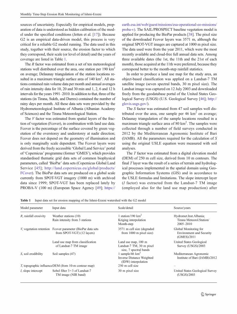
sources of uncertainty. Especially for empirical models, prep-aration of data is understood as hidden calibration of the mod-el under the specified conditions (Jetten et al. [17]). BecauseG2 is an empirical data-driven model, this process is verycritical for a reliable G2 model running. The data used in thisstudy, together with their source, the erosion factor to whichthey correspond, their scale (or level of detail) and the years ofcoverage are listed in Table 1.

The R factor was estimated from a set of ten meteorologicalstations well distributed over the area, one station per 190 km2

on average; Delaunay triangulation of the station locations re-sulted in a maximum triangle surface area of 140 km2. All sta-tions contained rain volume data per month and annual averagesof rain intensity data for 10, 20 and 30 min and 1, 2, 6 and 12 hintervals for the years 1991–2010. In addition to that, three of thestations (in Tirana, Sukth, and Durres) contained the number ofrainy days per month. All these data sets were provided by theHydrometeorological Institute of Albania (Albanian Academyof Sciences) and the Tirana Meteorological Station.

The V factor was estimated from spatial layers of the frac-tion of vegetation (Fcover), in combination with land use data.Fcover is the percentage of the surface covered by green veg-etation of the overstorey and understorey at nadir direction;Fcover does not depend on the geometry of illumination andis only marginally scale dependent. The Fcover layers werederived from the freely accessible ‘Global Land Service’ portalof ‘Copernicus’ programme (former ‘GMES’), which providesstandardised thematic grid data sets of common biophysicalparameters, called ‘BioPar’ data sets (Copernicus Global LandService [45]; http://land.copernicus.eu/global/products/FCover). The BioPar data sets are produced on a global scalecurrently from SPOT-VGT imagery (1000 m) with archiveddata since 1999; SPOT-VGT has been replaced lately byPROBA-V (100 m) (European Space Agency [49]; https://

earth.esa.int/web/guest/missions/esa-operational-eo-missions/proba-v). The SAIL/PROSPECT baseline vegetation model isapplied for producing the BioPar products [38]. The pixel sizeof the downloaded Fcover layers was 3571 m, although theoriginal SPOT-VGT images are captured at 1000 m pixel size.The data used were from the year 2011, which were the mostrecently available and cloud-free full annual data sets. Amongthree available dates (the 1st, the 11th and the 21st of eachmonth), those acquired at the 11th were preferred, because theycorrespond better to the month-step rainfall statistics.

In order to produce a land use map for the study area, anobject-based classification was applied on a Landsat-7 TMsatellite image (seven spectral bands, 30 m pixel size). TheLandsat image was captured on 12 July 2003 and downloadedfreely from the geodatabase portal of the United States Geo-logical Survey (USGS) (U.S. Geological Survey [46]; http://glovis.usgs.gov/).

The S factor was estimated from 47 soil samples well dis-tributed over the area, one sample per 46 km2 on average;Delaunay triangulation of the sample locations resulted in amaximum triangle surface area of 80 km2. The samples werecollected through a number of field surveys conducted in2012 by the Mediterranean Agronomic Institute of Bari(IAMB). All the parameters required for the calculation of Susing the original USLE equation were measured with soilanalyses.

The T factor was estimated from a digital elevation model(DEM) of 250 m cell size, derived from 10 m contours. Thefinal T layer was the result of a series of terrain and hydrolog-ical processes implemented in the spatial domain using Geo-graphic Information Systems (GIS) and in accordance tothe USLE formulas and limitations. The slope intercept layer(I factor) was extracted from the Landsat-7 TM image(employed also for the land use map production) after

Table 1 Input data set for erosion mapping of the Ishmi-Erzeni watershed with the G2 model

Model parameter Input data Scale/detail Source/years

R, rainfall erosivity Weather stations (10)Rain intensity from 3 stations

1 station/190 km2

Kriging interpolationMonth-step

Hydromet.Inst.Albania;Tirana Meteorol.Station/2005–2010

V, vegetation retention Fcover parameter (BioPar data setsfrom SPOT-VGT) (12 layers)

3571 m cell size (degradedfrom 1000 m pixel size)

Global Monitoring forEnvironment and Security(GMES)/2011

Land use map from classificationof Landsat-7 TM image

Land use map, 100 mLandsat-7 TM, 30 m pixelsize, 7 spectral bands

United States GeologicalSurvey (USGS)/2003

S, soil erodibility Soil samples (47) 1 sample/46 km2

Inverse Distance Weighted(IDW) interpolation

Mediterranean AgronomicInstitute of Bari (IAMB)/2012

T, topographic influenceDEM (from 10-m contour map) 250 m cell size –

I, slope intercept Sobel filter 3×3 of Landsat-7TM image (NIR band)

30 m pixel size United States Geological Survey(USGS)/2003

Monthly Time-Step Erosion Risk Monitoring of Ishmi-Erzeni

implementation of a non-directional edge detection filter onthe near-infrared band of the image.

2.4 Calculation of Erosion Factors

2.4.1 Rainfall Erosivity (R)

According to Wischmeier and Smith [40], the rainfall erosiv-ity factor (R) of a storm event is defined as the product ofstorm energy (En) times the maximum 30-min intensity(Imax30) of the event, where En can be calculated usingthe formula as follows:

En ¼ 210þ 89*log Imax30ð Þ ð2Þ

En is measured in tons per hectare and I in centimetre perhour; therefore, R units will be the following: ton centimetresper hectare per hour (ton cm ha−1 h−1). R values for a specificperiod of time are calculated as the sum of R of all events inthat period. However, in most cases, rain intensity figuresfrom individual events are rarely available, or the weatherstation networks are not dense enough in order to supportreliable R surfaces over large areas. On the other hand, alter-native empirical formulas based on rainfall volume (instead ofintensity) for deriving local to regional R spatial patterns, suchas the Arnoldus index ([11]; Duran Zuazo et al. [10]), havebeen criticised a lot if used in different areas from those forwhich they were originally developed [23].

Implementing the original USLE formulas on rain intensitydata from the weather station of Serres (northern Greece) re-corded during 1972–1987, Panagos et al. [28] found thatmonth-step distributions of R values derived for 15 min,30 min, 1 h, 2 h, 6 h, 12 h and 24 h were similar. Also,month-step distribution of R values that resulted from the im-plementation of the original USLE formulas using monthlyrain volume divided by the corresponding rainy hours (i.e. asimulated monthly intensity instead of Imax30) were similarwith the 2 h-based and the 6 h-based R distributions. Finally,calculation of R for January, April and May after replacingImax30 with the simulated monthly intensity resulted in R

values very close either to the 1 h- or 30 min-based R values.These findings allowed the modification of the original USLEformula by the G2 model, through the following:

& Replacement of Imax30 by simulated monthly intensity[28], a useful alternative when rainfall intensity data arelacking from a study.

& Introduction of a monthly storm factor (s), as compensa-tion for differentiations of rain intensity per month, whenrain intensity data are available only on an annual basis.Monthly storm factor is the ratio of simulated monthlyintensity over the annual average intensity.

The above modifications respond to the criticism of USLEfor not taking into account the volume of rainfall—but only theintensity—thus leading often to overestimations, especially atlow rates [19]. By replacing Imax30 by the simulated monthlyintensity, the G2 model emphasises the contribution of rainfallvolume in the equation. For the same reason, the rain intensityfactor is not contained in the calculation of R for a second time(as it does in the original USLE formula), thus rendering Ridentical to E (the total storm energy factor). Therefore, the Rformula for G2 has been modified from USLE, as follows:

R ¼ 524þ 222*log P=hð Þ ð3Þwhere, R is the rainfall erosivity of a specific month(MJ cm ha−1 h−1), P is the rainfall volume of the month (cm)and h is the number of rainy hours of the same month. In caseswhere rainy hours per month are not available, annual rainintensity can be used instead, with storm factor (s) differentiat-ing R per month; then, the R formula becomes as follows:

R ¼ s* 524þ 222*log Ið Þ½ � ð4Þ

where, R is as in Eq. (3), I is an annual rain intensity data set(cm h−1) and s is the monthly storm factor (normalised,dimensionless).

In the current study, rain intensity data were available forall the stations, but only annually averaged. Therefore, an

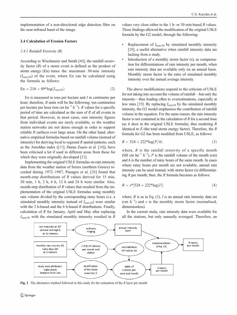
Fig. 2 The alternative method followed in this study for the estimation of the R layer per month

C.G. Karydas et al.

adequate site-specific distribution was possible, but not a tem-poral one, in terms of month-step values, as required by themodel. The solution followed is described below (Fig. 2):

& A single annual rain intensity layer for the whole studyarea was created using the 30 min interval figures avail-able at ten stations. As we were interested to capture theeffect of the climate change on erosion risk, we selectedonly 5 years of rainfall records (i.e. 2005–2010) ratherthan taking the full time series (i.e. 1991–2010). The or-dinary Kriging interpolation was applied for the creationof the rain intensity layer.

& A storm factor layer was created for every month; there-fore, 12 s layers were created. More specifically,

& First, the ratios of rain volume for every month over therainy hours of that month were calculated to produce thesimulated monthly intensities. Only rainfall events greaterthan 10 mm were taken into account, following the ap-proach ofWischmeier and Smith [40], who left out rainfalltotals lower than half an inch (12.7 mm) in the develop-ment of the USLE equation for R.

& Then, the monthly intensity values were divided by themean value of the set, in order to produce s (value range,0 to ∞). Because the intensity data were available only forthree stations (Tirana, Sukth, and Durres), the study areawas stratified into three zones (one per station) by group-ing those subwatersheds found closer to each of the sta-tions. For every month, the s layer was produced as aspatial union of the three zones. The s values for allmonths and stations ranged finally between 0.7 and 1.3(i.e. ±30 % around the mean).

& The R layers per month were created by implementing,Eq. (4).

2.4.2 Vegetation Retention (V)

Denoted asC factor, the vegetation coverage and managementfactor in USLE is the ratio of soil loss from land under aspecific vegetation management system to the correspondingsoil loss under continuous fallow. The C factor measures theeffect of all vegetation cover and management practicesthroughout a year and takes values from empirical tables[40]. Several alternative methodologies have been developedover time, such as the use of available land cover/use maps inorder to quantify the C factor, vegetation mapping with imageclassification techniques and field data, or the use of variousvegetation indices [39, 32]. Some of these methodologieshave been criticised for producing completely static outputsor for being based on very different sources [29], while others

for resulting in poor correlations with vegetation attributes,especially in the Mediterranean environments [39].

The G2 model has redefined vegetation coverage and man-agement factor and renamed it into V factor (after ‘vegetationretention’ because vegetation deters rain from reaching soilsurface). V factor estimation is based on Fcover, which is asimple biophysical parameter expressing the percentage of thesurface covered by green vegetation and is dimensionless. Inorder to refine a first rough estimation of V, G2 has also intro-duced a corrective land use parameter (LU), which empha-sises the influence of different land uses for similar values ofvegetation coverage. From the USLE experiments [40], it isimplied that C values change exponentially with crop cover,irrespective of the specific land use and management. Basedon these findings, the formula for V factor was determined asfollows [31]:

V ¼ e LU*Fcoverð Þ ð5Þwhere, V is the vegetation retention (normalised. dimension-less), with a V value equal to 1 for completely bare agriculturalland and V values larger than 1 for any better conditions;Fcover is a normalised value of vegetation cover fraction(range, 0–1); and LU is an empirical land use parameter rang-ing from 1 to 10, with lower values corresponding to moreintensive land use management (Fig. 3). A set of LU valueshas been defined through a combination of empirical dataavailable from USLE and EPM (Gavrilovic) models [31].

A land use map for the study area was derived from aLandsat-7 TM image after semi-automated classification(assisted by photo-interpretation) according to the CORINELC/LU nomenclature. Taking into account the lack of in situinformation, five broad land use categories were mapped inthe area:

Fig. 3 The family of exponential equations of V factor vs. Fcover fordifferent land uses

Monthly Time-Step Erosion Risk Monitoring of Ishmi-Erzeni

& Artificial surfaces, including settlements, transportation-sport-leisure facilities and green urban areas, with the ex-ception of mineral extraction sites, dump sites and con-struction sites, i.e. CORINE category 1 except subcate-gories 131, 132 and 133. These classes were assigned aLU value of 8.0, because they are mostly covered by im-pervious surfaces. The excluded classes were assigned aLU value of 1.0 [31, 32].

& Agricultural lands, including arable land, permanent cultiva-tions (such as olive plantations and vineyards) andrangelands (such as natural grasslands, moors-heathlandsand transitional woodland-shrub surfaces), with the excep-tion of agro-forestry areas, i.e. CORINE category 2 exceptsubcategory 244 and CORINE categories 321, 322 and 324.These classes were assigned a LU value of 4.5, because it isreported that inappropriate management practices of agricul-tural land and rangelands are predominant in the area [1].

& Broadleaved forests and sclerophyllous vegetation sur-faces, i.e. CORINE subcategories 311 and 323. Theseclasses were assigned a LU value of 7.0, considering amoderate degree of deforestation practices [1].

& Coniferous forests and mixed forests, i.e. CORINEsubcategories 312 and 313. These classes wereassigned a LU value of 4.0, as these forests areusually open forests at low altitudes, which alloweasy human intervention [1].

& Wetlands and water bodies, including lakes, sea and watercourses, i.e. CORINE categories 4 and 5. These categorieswere excluded from the assessment as non-erosive classes[1].

Object-based image analysis (OBIA) was performed withthe Landsat image using eCognition Developer© software;except for the Landsat image, no other data sources wereemployed. In OBIA, classification is implemented on previ-ously segmented images, in terms of division of an image intospatially continuous, disjoint and homogeneous regions,called image objects. Homogeneity reflects decomposabilityof natural systems into meaningful objects given that a re-maining internal heterogeneity within objects is explicitly ad-dressed [6]. The Fractal Net Evolution Approach (FNEA)(also known as ‘multi-resolution segmentation’) was applied.FNEA is an algorithm where the most determining factor ofobject size is the scale parameter, while the objects’ geometryis influenced by the degree in which spectral and shape infor-mation are weighted [2]. Through a trial-and-error procedure,a scale of 20 was found most appropriate to separate the studyarea into meaningful objects of different land uses; the ratio ofspectral to shape information for the segmentation was set to8/2.

The samples of image objects from the targeted classeswere collected by visual interpretation of the Landsat image.The nearest neighbour (NN) classification methodology was

applied on the image objects in a multidimensional space,comprising the following features:

& Normalised difference vegetation index (NDVI), which isa well-established index for classifying degrees of vegeta-tion abundance present in a land surface [16].

& Mean pixel value of objects in bands:

& 1 (the blue band of Landsat-7 TM), which is appropriatefor discriminating artificial surfaces due to high reflec-tance of concrete in blue wavelengths

& 7 (a middle infrared band of Landsat-7 TM), which isappropriate for recognising water bodies (even the veryshallow ones)

& Standard deviation of pixel values of objects in bands:

& 2 (green band of Landsat-7 TM), which is appropriate fordifferentiating natural from agricultural surfaces, due totheir different homogeneity degree in greenness;

& 6 (the thermal band of Landsat-7 TM), which was expect-ed to differentiate artificial from agricultural surfaces, dueto their difference in homogeneity degree in temperature.

The above selected features resulted in a minimum Euclid-ean distance of 0.461 in the multidimensional featurespace employed for the classification. The output thematicimage was then converted into vector format and was furtherimproved manually. According to the land use map resultingfrom the classification, the main land uses in the area can bedistributed approximately as follows: artificial surfaces95 km2 (4 %) agricultural land 1086 km2 (49 %), broadleavedforests 465 km2 (21 %), coniferous/mixed forests 524 km2

(24 %) and water bodies 35 km2 (2 %).Finally, Eq. (5) was implemented for each month, resulting

in a set of 12 V layers. In this study, the LU layer forced the Vlayer to downscale to a cell size of 200 m (a realistic value forland use discrimination) from 3571 m, which was the resolu-tion of the available Fcover layers. In other words, LU assistedfurther towards site specification of the V factor (Fig. 4).

2.4.3 Soil Erodibility (S)

In this study, the estimation of soil erodibility (denoted as Sfactor by G2, instead of K by USLE) was achieved byimplementing the original USLE formula. According toUSLE literature, the soil erodibility factor is defined as therate of soil loss per unit of R, as measured in a unit plot underspecific conditions (the so-called ‘Wischmeier plot’). Thisfactor accounts for the influence of soil properties on soillosses during storm events [33]. The equation of the USLEfor the K factor and thus for the S factor is as follows [40, 30]:

C.G. Karydas et al.

S ¼ 1:313* 10−4*2:1*M1:14* 12�OMð Þ þ 3:25* s−2ð Þ þ 2:5* p−3ð Þ� �

ð6Þ

where, S is the soil erodibility (t ha hMJ−1 ha−1 cm−1);M is thetexture from the upper 15 cm of the soil surface, calculated as(100−Ac)*(L+Armf), where Ac is the percentage of clay, L isthe percentage of silt and Armf is the percentage of very finesand; OM is the percentage of organic matter content, s is thestructure class of soil (s=1 for very fine granular, s=2 for finegranular, s=3 for medium or coarse granular and s=4 forblocky, platy or massive); and p is the permeability class of

the soil (p=1 for very rapid, p=2 for moderate to rapid, p=3for moderate, p=4 for slow to moderate, p=5 for slow, p=6for very slow).

Forty-seven samples from throughout the study area werecollected to create the S layer by spatial interpolation. Thefield survey was supported by the Mediterranean AgronomicInstitute of Bari (IAMB). The inverse distance weighted(IDW) method was applied. A mean S value of 0.1212 wasfound, with a minimum value of 0.0186 and a maximum valueof 0.2666. The soils were found to be more erodible in thewestern part of the study area, where the agricultural areas

Fig. 4 The V layer of Ishmi-Erzeni watershed forthe month April; the influence ofthe LU layer on the rough spatialpattern of Fcover layers is appar-ent (the eastern edge of the studyarea was excluded, as cloud-freeFcover layers for mostmonths were not available)

Fig. 5 The T layer of Ishmi-Erzeni watershed after maskingout areas with slope larger than14° (white areas)

Monthly Time-Step Erosion Risk Monitoring of Ishmi-Erzeni

dominate, than in the eastern mountainous part, with somelocal peaks found at the central part.

2.4.4 Topographic Influence (T)

The G2 model has adopted the method introduced by Mooreand Burch [25] for the estimation of topographic influence onerosion from a Digital Elevation Model (DEM). This methodallows for the calculation of convergent and divergent slopesand therefore for spatially distributed USLE applications. Ac-cording to Desmet and Grovers [8]), this method gives equiv-alent estimations with the original USLE formulas for slopeLength and Steepness (LS) factor. An alternative approachproposed by Mitasova et al. [24] requires very detailed inputDEMs (cell size smaller than 5 m), which was not available inthis application. Therefore, for the topographic influence (T

factor, equivalent to LS factor), the formula used by G2 is thefollowing:

T ¼ As=22:13ð Þ0:4* sinβ=0:0896ð Þ1:3 ð7Þ

where, T is the topographic influence (dimensionless), As isthe flow accumulation (m) and β is the slope steepness (rad).Flow accumulation is defined as the amount of flow from alupslope cells concentrating in a specific cell.

It has been shown that Eq. (7) is consistent with the originalUSLE equations for the calculation of the topographic factor(LS) only when slope length is less than 100 m and slopesteepness is less than 14° [26]. In order to meet the formercondition, G2 has introduced the I factor, which thus plays acorrective role to T. In order to meet the latter condition, G2excludes areas with a slope gradient larger than 14°; as aresult, these areas are not contained in the final erosion maps.In case of extensive areas with steep slopes, an alternative is todefine an equation of T vs. slope from a sample of represen-tative locations then determine the T value corresponding to14° (T14) and finally set T14 as an upper threshold for T values.

In this study, the T factor layer was calculated from theavailable DEM at 250 m resolution. In the flow accumulation(As) layer (produced by a series of steps supplied by the ‘Hy-drology’ module of ArcMap© software), null values (whichare expected to be along ridges) were set to one in order toavoid null T values, which in turn would result in null erosion.This was necessary, considering that a cell with As=0 mightcorrespond to β≠0. Also, the original As layer was multipliedby 250 in order to convert number of cells into metres, as isrequired by Eq. (7). The T values of cells falling into thedrainage network (streams/rivers), which are usually very

Fig. 6 The influence of Sobel filter on erosion, in terms of relativeerosion reduction; Sobel values calculated according to Eq. (8) (hereDNmax=255)

Fig. 7 The annual erosionmap ofIshmi-Erzeni, resulting from theaccumulation of the month-stepmaps (white for no data)

C.G. Karydas et al.

high, were set to 0, as they are non-erosive areas, or sheet-interrill erosion is not-applicable there. Finally, all the areaswith slope larger than 14° were masked out (Fig. 5).

2.4.5 Slope Intercept (I)

The G2 model has introduced a corrective parameter to the Tfactor, which is called ‘slope intercept’ and is denoted as Ifactor. This factor expresses the effect of linear landscape fea-tures on erosion, considering that these features have the

potential to intercept rainfall runoff by reducing the slopelength. In order to recognise and map linear landscape fea-tures, a Sobel filter is applied on a medium-high resolutionmultispectral satellite image (approx. 20 to 30 m pixel size).The Sobel filter is a common non-directional edge detectionfilter, with the coefficients designed to add up to zero(Richards and Jia [34]).

Features that are expected to be captured by the Sobel filter(and thus provide the highest output values) include roads,paths or natural strips between parcels, hedges, fences and

January February March

April May June

July August September

October November December

t/ha

0 - 0.5

0.5 - 1

1 - 2

2 - 5

5 - 10

10 - 20

> 20

Fig. 8 Time series of erosion maps of Ishmi-Erzeni watershed derived with the G2 model (white for no data)

Monthly Time-Step Erosion Risk Monitoring of Ishmi-Erzeni

terrace steeps. All these features are very likely to interceptrainfall runoff and thus protect soil from erosion acceleration.The Sobel filter is implemented on the near-infrared band of amultispectral satellite image using a 3×3 moving window. Asof textural nature, Sobel image is by default normalised andthus comparable to other Sobel images.

G2 has proposed the following formula for the conversionof Sobel values into slope intercept values (the revised ver-sion, [31]):

I ¼ 1þ √ S f =DNmax

� � ð8Þ

where, I is the slope intercept value (dimensionless; range, 1–2); Sf is the Sobel 3×3 filter value ranging in 0–DNmax andDNmax is the maximum digital number of the Sobel image(e.g. 255 for an 8-bit image data set). As it is perceived from

Eq. (8), the influence of I factor on erosion will be a non-linear one. In other words, erosion will be reduced by a higherrate for the low range of Sf values and by a lesser rate as Sfvalues increase (Fig. 6). As a result, the reduction of erosion isexpected to be always less than 50 %. This option is justifiedby the following facts:

& Erosion is a dynamic phenomenon. If some features areexpected to reduce runoff, extra features will influence analready reduced erosion rate; therefore, their effect will beless significant.

& The I layer expresses the effect of the landscape only onthe runoff component of erosion processes. Therefore, soilloss from raindrop splash and runoff at very short dis-tances (e.g. within a pixel) are not affected by any inter-cept feature (captured by the image).

& Finally, I is a parameter only partially corrective to T, i.e.the major effect of the terrain has already been calculated,while effects from other conservation measures are ele-ments of the V factor (through the LU parameter).

Implementation of Eq. (8) in the study area resulted in Ivalues ranging between 1 and 1.67, with a mean value at 1.17.This means that the current landscape heterogeneity has re-sulted in a reduction of erosion by about 15 % on average.

3 Results and Discussion

The outputs of the G2 model implementation in the Ishmi-Erzeni watershed comprise a set of maps, such as the 12month-step erosion maps, the annual erosion map and 12

Fig. 9 Temporal figures of R, V and E for the entire Ishmi-Erzeni water-shed (normalised to the minimum value, logarithmic scale)

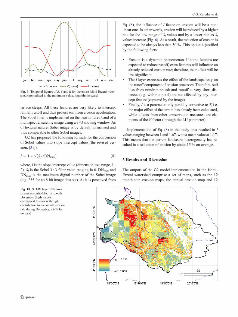
Fig. 10 STERI layer of Ishmi-Erzeni watershed for the monthDecember (high valuescorrespond to sites with highcontribution to the annual erosionrate during December; white forno data)

C.G. Karydas et al.

month-stepmaps of relevant contribution to the annual erosion;also, several graphs are derived showing the annual evolutionof rainfall, vegetation and erosion means on a month-step.

The mean annual erosion rate was found to be 6.5 t/ha. Themaximum annual value was found to be 215 t/ha, the mini-mum 0 t/ha and the standard deviation 12.9 t/ha; the coeffi-cient of variation was estimated at 197 %. The calculated rateshave been verified by sediment transport findings ofGrazhdani and Shumka [14], who were the first to map ero-sion in the whole Albania on a time-step of a month. Thevalues of our erosion maps were classified into seven riskclasses in accordance to the ‘PESERA’ project, which hasproduced a pan-European erosion risk map [20], so as to makeerosion maps comparable. The same classification has alsobeen followed in the Strymonas and Crete applications ofthe G2 model (Fig. 7).

With regard to annual erosion rates, 18 % of the mappedarea was found to be at risk of annual soil losses larger than10 t/ha, a value considered to be non-sustainable in Albania,according to Grazhdani and Shumka [14]. Wischmeier andSmith [40] have reported values between 4.5 and 11 t/ha/yearas sustainable upper thresholds for different US agriculturallands. An exploration of the spatially lumped maximum,

minimum and mean results of erosion (in t/ha) together withR and V figures on a month-step can lead to some first notifi-cations about the annual cycle of soil erosion risk in the Ishmi-Erzeni watershed (Figs. 8 and 9):

& November, December, January and February were themost erosive months (with more than 0.7 t/ha each) withMarch following (0.64 t/ha).

& April and October were moderate in erosion rates (lessthan 0.5 t/ha).

& Erosion rates were found to be low in June and July (lessthan 0.4 t/ha).

& May was found to be the least erosive month in the area(0.27 t/ha).

In summary, the winter and autumn months seem to bemore risky than spring and summer ones. More specifically,winter and autumn months account for about two thirds of theannual erosion rates (33 and 30 %, respectively), whereasspring and summer months account for the remaining onethird (20 and 17 %, respectively). All months contributedbetween 4 and 12 % to the annual rates. Generally, themonth-stepmaps gave analogous spatial patterns to the annual

Fig. 11 An example of annual erosion risk overlaid by land use polygons; coniferous and mixed forests are showed in stripped lines (white cells for nodata); a close view

Monthly Time-Step Erosion Risk Monitoring of Ishmi-Erzeni

erosion map. Also, it was showed that month-step erosionrates were mostly influenced by temporal distribution of veg-etation, rather than rainfall patterns.

Month-step outputs provided by the G2 model allow forthe definition of a relative risk index in terms of contributionof each month to the annual erosion risk either for the entiremapped area or for a specific site. This index is called ‘spatio-temporal erosion risk index’ (STERI) and has been defined byPanagos et al. [31], as follows:

STERIn ¼ En=E ð9Þ

where, STERIn is the spatio-temporal erosion risk index(dimensionless) for month n, En is the erosion value for monthn and E is the annual erosion value. For example, a rate of0.2 t/ha in January at a specific site (cell or group of cells),where the annual rate for the same site is 0.8 t/ha, will result ina STERI value of 0.25, which means that 25 % of the annualerosion at the specific site occurs in January (Fig. 10).

With regard to the different land uses found in the area,coniferous and mixed forests appear to give the highest riskfor erosion. This can be partially attributed to theirparticularities with regard to the landscape, such as steepslopes in which they usually are grown and their low vegeta-tion density, i.e. their sparse leave area and the wide openspaces among the coniferous trees (Fig. 11). On the otherhand, broadleaved forests did not coincide with the highesterosion risk class, but only partially; these forests were foundin the medium-risk categories for erosion. Agricultural landswere generally found in low risky areas, as they usually coverplain areas. However, agricultural lands in sloppy mountain-ous sites express a medium to high risk for erosion.

The results of G2 in the Ishmi-Erzeni watershed could notbe validated in the absence of soil loss measurements fromexperimental field plots and/or site-specific sediment deliveryto watercourses for the study area, or any other similar area inAlbania.

4 Conclusions and Outlook

Using the G2 model, estimated soil loss for the Ishmi-Erzeniwatershed, Albania, was mapped. Moreover, the most criticalmonths were identified for five broad land use categories. Thequantitative outputs (t/ha) were used for identifying criticalsites, seasons and land uses. Also, they could be used forcomparisons with past or future assessments.

The G2 model was proved to be flexible enough in fittingthe alternative algorithms supported by the model to the avail-able data sets. It was also proved to be efficient for this study,as it provided all the expected outputs in a clear, systematicand robust manner. Therefore, the G2 model could be used as

a tool for supporting decision making in the Ishmi-Erzeniwatershed.

Soil erosion in Ishmi-Erzeni area was found to be moderateon average, but exceeding sustainable limits in several cases,especially for coniferous and mixed forests and agriculturallands in mountainous regions. The latter should be taken as analarm for preventing from abandonment of sloping lands, de-forestation, uncontrolled logging, overgrazing and forest fires(note catastrophic events of summer 2012).

This study is the third application of the G2model after thatof Strymonas and Crete applications. As a model which em-ploys standardised geodatabases and offers alternatives ac-cording to data availability, the G2 model is currently receiv-ing broad attention. Recently, the G2 model was applied inKorce region in Albania and in Cyprus; these studies are underreview for publication. Also, implementation of G2 on acountry-wide scale is underway in case of Albania andGreece.

Acknowledgments The authors wish to thank the Joint Research Cen-tre, Institute for Environment and Sustainability, Land Resource Manage-ment Unit and especially Dr. Panos Panagos, for hosting the G2 modelutilities and databases on the ESDB web portal (http://eusoils.jrc.ec.europa.eu/library/themes/erosion/G2/data.html). Also, we wish to thanktheMediterraneanAgronomic Institute of Bari (IAMB) for supporting thesoil sampling field survey and the Hydrometeorological Institute of Al-bania and the Tirana Meteorological Station for providing the weatherdata sets. Finally, we cordially thank Prof. Robert Jones, retired fromCranfield University, UK, for his diligent English review of the manu-script and to the anonymous reviewers, whose comments and suggestionsimproved the manuscript substantially.

References

1. Adlington, G. P. (2014). Albania—Land Administration andManagement Project (LAMP): P096263—implementation statusresults report: sequence 15. Washington, DC: World Bank.

2. Baatz, M., Benz, U., Dehghani, S., Heynen, M., Hotlje, A.,Hofmnn, P., Lingenfelder, I., Mimler, M., Sohlbach, M., Weber,M., and Willhauck, G. (2002). ECognition User’s Guide(Munich, Germany: Definiens Imaging GmbH), digital.

3. Banwart, S. (2011). Save our soils. Nature, 474, 151–152. doi:10.1038/474151a.

4. Baveye, P. C., Rangel, D., Jacobson, A. R., Laba, M., Darnault, C.,Otten, W., Radulovich, R., & Camargo, F. (2011). From dust bowlto dust bowl: soils still a frontier of science. Madison: CSA News.

5. Borselli, L., Torri, D., Poesen, J., & Iaquinta, P. (2012). A robustalgorithm for estimating soil erodibility in different climates.CATENA, 97, 85–94.

6. Burnett, C., & Blaschke, T. (2003). A multi-scale segmentation/object relationship modelling methodology for landscape analysis.Ecological Modelling, 168, 233–249.

7. Demiraj, E., Bicja, M., Gjik, E., Gjiknuri, L., Gjoka Mucaj, L.,Hoxha, F., Hoxha, P., Karadumi, S., Kongoli, S., Mullaj, A.,Mustaqi, V., Palluqi, A., Ruli, E., Selfo, M., Shehi, A., and Sino,Q. (1996). Implications of climate change for the Albanian Coast.MAP Technical Reports Series No.98, UNEP, Athens EuropeanCommunity. EIW Workshop: Elaboration of a Framework of a

C.G. Karydas et al.

Code of Good Agricultural Practices, Brussels, pp. 21–22,May 1992.

8. Desmet, P., & Grovers, G. (1996). A GIS procedure for automati-cally calculating the USLE LS factor on topographically complexlandscape units. Journal of Soil and Water Conservation, 51(5),427–433.

9. Driesen, P. M. (1986). Erosion hazards and conservation needs as afunction of land characteristics and land qualities. In W. Siderius(Ed.), Land evaluation for land-use planning and conservation insloping areas (pp. 32–39). ILRI: The Netherlands.

10. Duran Zuazo, V. H., Aguilar Ruiz, J., Martinez Raya, A., & FrancoTarifa, D. (2005). Agriculture, Ecosystems and Environment,107(2–3), 199–210.

11. Ferro, V., & Porto, P. (1999). A comparative study of rainfall ero-sivity estimation for southern Italy and southeastern Australia.Hydrological Sciences—Journal—des Sciences Hydrologiques,44(1), 3–24.

12. Foster, G.R. and Meyer, L.D. (1972). A closed-form soil erosionequation for upland areas. In: H.W. Sten, ed. Sedimentation sym-posium in Honor Prof. H.A. Einstein. Fort Collins, CO: ColoradoState University, 12.1_12.19.

13. Gavrilovic, Z. (1988). The use of an empirical method (erosionpotential method) for calculating sediment production and transpor-tation in unstudied or torrential streams. In: International conferenceof river regime, 18–20 May 1988, Wallingford. Chichester: JohnWiley and Sons, 411–422.

14. Grazhdani, S., & Shumka, S. (2007). An approach to mapping soilerosion by water with application to Albania. Desalination, 213(1–3), 263–272.

15. Grimm, M., Jones, R. J. A., Rusco, E., & Montanarella, L. (2003).Soil erosion risk in Italy: a revised USLE approach. EuropeanCommission, EUR 20677 EN, (2002), p. 28. Luxembourg: Officefor Official Publications of the European Communities.

16. Guyot, G., Baret, F., & Jacquemoud, S. (1992). Imaging spectros-copy for vegetation studies. In F. Toselli & J. Bodechtel (Eds.),Imaging spectroscopy: fundamentals and prospective applications(pp. 145–165). Dordtrecht: Kluwer Academic Publishing.

17. Jetten, V., de Roo, A., & Favis-Mortlock, D. (1999). Evaluation offield-scale and catchment-scale soil erosion models. Catena, 37(3–4), 521–541.

18. Karydas, C. G., Panagos, P., & Gitas, I. Z. (2014). A classificationof water erosion models according to their geospatial characteris-tics. International Journal of Digital Earth, 7(3), 229–250.

19. Kinnel, P. I. A. (2003). Event erosivity factor and errors in erosionpredictions by some empirical models. Australian Journal of SoilResearch, 41(5), 991–1003.

20. Kirkby, M. J., Irvine, B. J., Jones, R. J. A., & Govers, G. (2008).The PESERA coarse scale erosion model for Europe. I.—modelrationale and implementation. European Journal of Soil Science,59(6), 1293–1306.

21. Laze, P. and Kovaci, V. (1996). Soil erosion and physico-chemicalnature of eroded materials. 9th Conference of the International SoilConservation Organization (ISCO), Bonn, Germany. ExtendedAbstracts.

22. Laze, P., Suljoti, V., Kovaci, P. and Brahushi, F. (2005). ThematicAssessment Report Land Degradation and Desertification. UnitedNations Convention to Combat Desertification. Tirana.

23. Marker, M., Angeli, L., Bottai, L., Costantini, R., Ferrari, R.,Innocenti, L., & Siciliano, G. (2008). Assessment of land degrada-tion susceptibility by scenario analysis: a case study in SouthernTuscany, Italy. Geomorphology, 93(1–2), 120–129.

24. Mitasova, H., Hofierka, J., Zlocha, M., & Iverson, R.(1996). Modelling topographic potential for erosion and de-position using GIS. International Journal of GIS, 10(5),629–641.

25. Moore, I. D., & Burch, G. J. (1986). Physical basis of the length-slope factor in the universal soil loss equation. Soil Science SocietyAmerica Journal, 50, 1294–1298.

26. Moore, I. D., & Wilson, J. P. (1992). Length-slope factors for theRevised Universal Soil Loss Equation: simplified method of esti-mation. Journal of Soil and Water Conservation, 4(5), 423–428.

27. Oldeman, L.R., Hakkeling, R.T.A., and Sombroek, W.G. (1991).World map of the status of human-induced soil degradation: anexplanatory note. Wageningen: International Soil Reference andInformation Centre; Nairobi: United Nations EnvironmentProgramme.

28. Panagos, P., Karydas, C. G., Gitas, I. Z., &Montanarella, L. (2012).Monthly soil erosion monitoring based on remotely sensed bio-physical parameters: a case study in Strymonas river basin towardsa functional pan-European service. International Journal of DigitalEarth, 5(6), 461–487.

29. Panagos, P., Van Liedekerke, M., Jones, A., & Montanarella, L.(2012). European Soil Data Centre (ESDAC): response toEuropean policy support and public data requirements. Land UsePolicy, 29(2), 329–338.

30. Panagos, P., Meusburger, K., Alewell, C., & Montanarella, L.(2012). Soil erodibility estimation using LUCAS point survey dataof Europe Environmental. Modelling and Software, 30, 143–145.

31. Panagos, P., Karydas, C., Ballabio, C., & Gitas, I. (2014). Seasonalmonitoring of soil erosion at regional scale: an application of the G2model in Crete focusing on agricultural land uses. InternationalJournal of Applied Earth Observation and Geoinformation,27(B), 147–155.

32. Panagos, P., Karydas, C. G., Borrellia, P., Ballabio, B., &Meusburger, K. (2014). Advances in soil erosion modellingthrough remote sensing data availability at European scale.Proceedings of SPIE, 9229, 92290I.

33. Renard, K. G., Foster, G. R., Weesies, G. A., McCool, D. K., &Yoder, D. C. (1997). Predicting soil erosion by water: a guide toconservation planning with the revised universal soil loss equation(RUSLE) (agricultural handbook 703) (p. 404). Washington, DC:US Department of Agriculture.

34. Richards, J. A., & Jia, X. (1999). Remote sensing digital imageanalysis. Heidelberg: Springer.

35. Rusi, M., Xhomo, A., and Rusi, S. (2006). Perdorimi i burimevenatyrore te reja per perfitimin e gurit gelqeror per nevojat e sektoritte ndertitmit dhe infrastruktures eshte domosdoshmeri dhe prioritetper ruajtjen e ambjentit. Qendra per kerkim dhe zhvillim (QKZH).Tirane, pp. 47–67.

36. Scherr, S.J. and Yadav, S. (1996). Land degradation in the develop-ing world: implications for food, agriculture and the environment to2020. Food, Agriculture, and the Environment Discussion Paper14, Washington DC: International Food Policy Research Institute.

37. Van der Knijff, J. M., Jones, R. J. A., & Montanarella, L. (1999).Soil erosion risk assessment in Italy. European Soil Bureau. Italy:European Commission, JRC Scientific and Technical Report, EUR19044 EN, p. 52.

38. Verhoef, W. (1985). Earth observation modeling based on layerscattering matrices. Remote Sensing of Environment, n., 17, 165–178.

39. Vrieling, A. (2006). Satellite remote sensing for water erosion as-sessment: a review. Catena, 65(1), 2–18.

40. Wischmeier, W.H. and Smith, D.D. (1978). Predicting rainfall ero-sion losses: a guide for conservation planning (AgricultureHandbook 537), US Department of Agriculture.

41. Yang, D., Kanae, S., Oki, T., Koike, T., & Musiake, K. (2003).Global potential soil erosion with reference to land use and climatechanges. Hydrological Processes, 17, 2913–2928.

42. Zdruli, P. and Lushaj, Sh. (2012). Problems of soil degradationand alternative control measures for soil protection in Albania.

Monthly Time-Step Erosion Risk Monitoring of Ishmi-Erzeni

Poster presentation, Book of Abstracts. EUROSOIL2012, Bari,Italy.

43. Zdruli, P., Lushaj, Sh., Pezzuto, A., Fanelli, D., D’Amico, O.,Filomeno, O., De Santis, S., Todorovic, M., Nerilli, E., Dedaj, K.,and Seferi, B. (2003). Preparing a georeferenced soil database forAlbania at scale 1:250,000 using the European Soil Bureau Manualof Procedures 1.1. In: 7th International Meeting on Soils withMediterranean Type of Climate, Selected Papers. OPTIONSméditerranéennes (Eds. Zdruli, Steduto and Kapur). Series A:Mediterranean Seminars No. 50. Bari, Italy. ISBN 2-85352-248-2.

Electronic sources

44. European Union (COM2012 46 final), http://ec.europa.eu/environment/soil/three_en.htm (last accessed: March 2015).

45. Copernicus programme, Global Land Service, http://land.copernicus.eu/global/products/FCover (last accessed:March 2015).

46. United States Geological Survey (USGS), 2011. GeographicInformation System, http://glovis.usgs.gov/ (last accessed:March 2015).

47. WMO (World Meteorological Organization)(2007). Climate andLand Degradation Workshop, http://www.wmo.int/pages/prog/wcp/agm/meetings/wocald06/background_wocald06.php (lastaccessed: March 2015)

48. UNCCD (United Nations Convention to Combat Desertification),2012. World Food Day 2012, Message of the UNCCD Secretary,UNCCD, Bonn, Germany, http://www.unccd.int/en/media-center/MediaNews/Pages/highlightdetail.aspx?HighlightID=133 (lastaccessed: March 2015).

49. European Space Agency (ESA), 2015; https://earth.esa.int/web/guest/missions/esa-operational-eo-missions/proba-v (last accessed:March 2015).

C.G. Karydas et al.