PROOF COPY [EM10594] 178005PRE

PROO

F COPY [EM

10594] 178005PREParticle-based model to simulate the micromechanics of biological cells

P. Van Liedekerke,* E. Tijskens, and H. RamonDepartment of BIOSYST, KULeuven, Leuven, Belgium

P. Ghysels, G. Samaey, and D. RooseDepartment of Computer Science, KULeuven, Leuven, Belgium

�Received 16 December 2009; revised manuscript received 4 May 2010�

This paper is concerned with addressing how biological cells react to mechanical impulse. We propose aparticle based model to numerically study the mechanical response of these cells with subcellular detail. Themodel focuses on a plant cell in which two important features are present: �1� the cell’s interior liquidlike phaseinducing hydrodynamic phenomena, and �2� the cell wall, a viscoelastic solid membrane that encloses theprotoplast. In this particle modeling framework, the cell fluid is modeled by a standard smoothed particlehydrodynamics �SPH� technique. For the viscoelastic solid phase �cell wall�, a discrete element method �DEM�is proposed. The cell wall hydraulic conductivity �permeability� is built in through a constitutive relation in theSPH formulation. Simulations show that the SPH-DEM model is in reasonable agreement with compressionexperiments on an in vitro cell and with analytical models for the basic dynamical modes of a spherical liquidfilled shell. We have performed simulations to explore more complex situations such as relaxation and impact,thereby considering two cell types: a stiff plant type and a soft animal-like type. Their particular behavior�force transmission� as a function of protoplasm and cell wall viscosity is discussed. We also show that themechanics during and after cell failure can be modeled adequately. This methodology has large flexibility andopens possibilities to quantify problems dealing with the response of biological cells to mechanical impulses,e.g., impact, and the prediction of damage on a �sub�cellular scale.

DOI: XXXX PACS number�s�: 87.17.Rt, 87.85.gp, 87.16.Gj

I. INTRODUCTION

Cellular systems—nature’s building blocks—are one ofthe most studied systems because these microscopic unitscontrol the overall macroscopic behavior of animals andplants. With respect to their mechanics, plant cells are intu-itively somewhat simpler than animal cells, since the formerare mostly immobilized. Nevertheless, the physical nature ofplant tissue remains challenging. It is intrinsically multiscaleas it depends on the microstructure of the cells as well as ontheir structural arrangement �aggregate level�. In addition, itis also a multiphysics problem, since apart from the im-mersed solid materials �e.g., cell wall, middle lamella�, fluidand gas transport in the cells, through the cell walls and inthe intercellular spaces, will play a role as well. In this re-spect the mechanics of plant tissue is considerably morecomplicated than other cellular materials such as metallicfoams and trabecular bone, where a single material is themain load-bearing component.

Plant cells usually have a strong cell wall to protect themfrom hostile environments. Inside these cells, a quasi-incompressible liquid builds up a hydrostatic pressure �turgorpressure� through osmosis which is responsible for the cel-lular rigidity �wilting of low hydrated plants�. The cellularmechanics in plants influences “slow” physiological pro-cesses inside the cell such as growth, development and mostlikely even gene expression �1–4�. It also plays a key role in

short time scale processes such as bruise formation in fruitduring impact and rapid plant movement in Venus Flytraps.Because of the difficulty to probe physical quantities at suchscale experimentally, the microscopic subcellular mechanicsthat goes along with these processes remains for a great partuncomprehended and unquantified �5–7�.

Therefore, in the past, relevant analytical models havebeen proposed to simulate the mechanics of cellular systems�8–14�, yet with limited flexibility and applicability. Othershave introduced finite element modeling �FEM�, consideringthe elastic quasistatic response of a cell �15,16�, or particleapproaches, focusing more on the rheological properties�17�. Nevertheless, to get more insight in the micromechani-cal response of cellular systems, it remains essential to de-velop models which can capture and describe more subcel-lular detail, including differences in cell shapes and sizes,and the intercellular interactions �18,19�.

This paper is concerned with building a model that candescribe the mechanics of a cell in static and dynamic situ-ations. To this end, we introduce a particle based method andfocus on spherical shaped plant cells whereby a solid phaseand a liquid phase are considered. Our approach is a combi-nation of smoothed particle hydrodynamics �SPH� to modelthe liquid phase and a discrete element method �DEM� todescribe the solid phase of the cell walls �6�. SPH is a maturemesh-free simulation method typically used in situationsdealing with large deformations, discontinuities, and freeboundaries. Originally developed in astronomical contexts�20�, it has now become a versatile technique in modelinggas and fluid dynamics. The choice to apply SPH in bio-logical systems lies also in the possibilities of modelingnon-Newtonian liquids, viscoelastic liquids, water transportin porous media, multiphase flow, and diffusion �see, e.g.,

*Corresponding author. Present address: Department of BIO-SYST, KULeuven, Kasteelpark Arenberg 30, Leuven, Belgium;paul.vanliedekerke@biw.kuleuven.be

PHYSICAL REVIEW E 81, 1 �2010�

1

23

456

789

101112131415161718192021

22

23

24

25262728293031323334353637383940414243444546474849

505152535455565758596061626364656667686970717273747576777879808182

1539-3755/2010/81�6�/1�15� ©2010 The American Physical Society1-1

PROOF COPY [EM10594] 178005PRE

PROOF COPY [EM10594] 178005PRE

PROO

F COPY [EM

10594] 178005PRE�21–23��. Furthermore, mesh-free particle methods are quitesuitable for coarse-graining and multiscaling approaches�24�. For example, the recent modeling technique smootheddissipative particle dynamics �SDPD� couples the hydrody-namic interactions of SPH with thermal fluctuations in athermodynamically consistent way �25–27�. Such formalismis useful in coarse-grained models of subcellular processeswhere these fluctuations become important.

The presented model here is primarily meant to predictforce transmission and stresses in biological cells. We con-sider a parenchyma cell, which makes the bulk of plant tis-sue, and can be mechanically regarded as a stiff, thin walledvessel �the cell wall� containing a viscous fluid. The systemas a whole is regarded as incompressible and isothermal. Thefocus is on short time scales, typically those arising at im-pact, where most long-term physiological responses are neg-ligible. Due to the adaptivity and flexibility of the particleframework, this cell-centered approach can be extended add-ing other cells to form a multicellular system �6�, supplyingrepresentative volume elements for computational homog-enization to obtain tissue constitutive behavior �28,29�. Onthe other side, it can also be refined to capture the detail ofthe subcellular structure.

In the following, we give a detailed description of themodel and compare it with the results of an analytical modeland an experimental test case on an in vitro cell during qua-sistatic compression. Thereafter, we introduce two cell types:a stiff type, resembling a plant cell; and a soft type, whichmimics a mammalian cell. We compare and discuss the re-laxation times of these types. Simulations of impact with aplate are performed, and we treat the arising intracellularstresses and intercellular stresses �transmitted forces� in moredetail. Finally, we show that this model is able to capture thefailure dynamics of a cell.

II. METHODOLOGY

A. Cell fluid model

Parenchyma cells are typically thin walled cells that retaintheir content. By removing the stiff cell wall, on obtains aprotoplast which is a soft heterogeneous substance contain-ing water, membranes, a nucleus, organelles, macromol-ecules, ions, and a cytoskeleton. The latter causes that theprotoplasm �30� �the living content of the cell� usually be-haves like a gel-like liquid. However, in parenchyma largevacuoles are present which serve as containers for the stor-age of water �up to 80–90 % of the cell’s volume �4�� and inaddition, these cells do not have the dense cytoskeleton likein animal cells. Therefore, we will preliminary assume thatthe protoplasm is a Newtonian homogeneous liquid whichcan be described by the Navier-Stokes �NS� equations.

In SPH, the particle approximation of a function evalua-tion f�xi� using a set of neighboring particles j can be writtenas

f�xi� � �j

V j f�x j�Wij , �1�

where xi is the position of the particle, and Vi is the volumeoccupied by one particle. The approximation function is a

kernel Wij �W�q ,s� were q=rij /s, rij is the distance from aparticle i to another fluid particle j, and s is the smoothinglength, representing the domain over which the particle i hasinteraction with particles j. It is symmetrical, i.e.,

Wij = Wji, �2�

and should be normalized,

�V

WdV = 1. �3�

In this paper, we choose the cubic spline function W�q ,s� asa kernel function, which reads

W�q,s� =2

3�s32

3− q2 +

1

2q3 0 � q � 1

1

6�2 − q�3 1 � q � 2

0 q � 2. �4�

In NS, the force Fi on a particle can be decomposed in apressure driven and a viscous component. Correspondingly, afluid particle i is moving according to a standard SPH ap-proximation of NS for a set of surrounding particles j

Fi = − mi�j

mj�Pi

�i2 +

Pj

� j2��iWij

+ mi�j

mj��i + � j

�i� j�vij

1

rij

�Wij

�rij, �5�

where P is the pressure of the fluid particle, m is its mass, �is the density, � is the dynamic viscosity and furthermorevij =vi−v j denotes the relative particle velocity. Kernels ofhigher order and kernel corrections may be used to improvethe accuracy or stability of the method �31,32�.

In the weakly compressible SPH method, it is convenientto use the following equation of state �EOS� �33� to maintaina relation between the pressure and the density,

P = P0 + � � �

�0�7

− 1� , �6�

where P0 is the initial net pressure �turgor� across the cell, �0

is the initial density of the fluid, and �=�0c2

7 is the compres-sion modulus where c is the speed of sound of the medium.Through Eq. �6�, variations in density will be penalized byincreasing the pressure, thus make the fluid weakly com-pressible. To update the density, we use the SPH approxima-tion of the continuity equation

d�i�

dt= �

j

mjvij . �iWij = mi�j

vij . �iWij , �7�

where �i� represents the density assuming a constant particle

mass. The general definition of density reads of course

�i =mi

Vi. �8�

The time derivative of Eq. �8� yields

VAN LIEDEKERKE et al. PHYSICAL REVIEW E 81, 1 �2010�

8384858687888990919293949596979899

100101102103104105106107108109110111112113114115116

117

118

119120121122123124125126127128129130131132133134

135

136137

138139140141

142

143

144

145146

147

148149150151

152

153

154155156157158159160161

162

163

164165166167168169

170

171172

173

174

1-2

PROOF COPY [EM10594] 178005PRE

PROOF COPY [EM10594] 178005PRE

PROO

F COPY [EM

10594] 178005PREd�i

dt= mi

d

dt� 1

Vi� +

1

Vi

dmi

dt=

d�i�

dt+

�i

mi

dmi

dt. �9�

Equation �9� can be interpreted as follows. The first term isthe change in density due to the deformation of the cell vol-ume, given by Eq. �7�, while the second term in Eq. �9� canbe attributed to a change in water content of the cell. Sinceplant cells have semipermeable walls, a net transport of wa-ter through the cell wall will be established as long as theturgor pressure in the cell does not equal the osmotic poten-tial ����0� of the cell content. If the cell fluid mass loss orgain is not too high, � can be assumed constant. This fluidmass transport through the cell wall can be computed foreach particle by the following constitutive relation �4�:

dmi

dt= −

AcLp�i

Nf�Pi + �� , �10�

where Lp is the hydraulic conductivity which is assumed tobe isotropic over the cell’s surface, Nf is the number of fluidparticles, and Ac is the total cell surface. If the cell absorbswater, the density will initially increase according to the lastterm in Eq. �9�, and hence augment the pressure by Eq. �6�.This is counterbalanced by the fact that the fluid will pushthe cell wall outward, thus, lowering the density. The finaldensity, which should differ only slightly from the initialdensity, will be obtained when the fluid particles cease tomove further, i.e., when there is a force balance between thefluid pressure and the cell wall stress.

B. Cell wall model

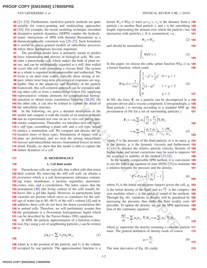
A plant cell wall is a polymerlike structure which princi-pally cannot be described by simple linear elasticity theory.Mechanically, the cell wall material exhibits elastic and plas-tic behavior and energy dissipation can be attributed to vis-cous and structural damping. This behavior further stronglydepends on the time scale �34�. On short time scales how-ever, in which the material composition can be assumed con-stant, the cell wall can be seen as a thin shell structure, de-scribed by a hyperelastic or elastoviscoplastic constitutivelaw. In this paper, we employ a DEM procedure in whichparticles are distributed on a surface, having a local connec-tivity and interacting through discrete forces. We implementthe simplest model to describe a polymer: the isotropic in-compressible Neo-Hookean solid. Our ansatz is a sphericalshell whereby the particles are positioned on the verticesobtained by triangulating its surface using icosahedral sym-metry. These form a net of nodes with sixfold connectivity�bonds� and contain 12 so-called topological defects with afivefold connectivity. All the particles have discrete elasticinteraction forces fe and a linear damping force fv to accountfor the viscous effects. Particles which are not bonded �nofixed connectivity� are subjected to excluded volume inter-actions fr to avoid interpenetration with other wall particlesand fluid particles �see Fig. 1�a��. The force law proposed forthese interactions is similar to a Lennard-Jones �LJ� poten-tial. The force on a cell wall particle i due to other cell wallparticles �j ,k� can be written as

fi = fe + fv + fr = �j

fije − �

j

�vij + �k

fkrik + �k

fk�vik,

�11�

with

fk = f0 � r0

rik�8

− � r0

rik�4� 1

rik2 . �12�

The summation in Eq. �11� is taken over all bonded �j� andall nonbonded �k� particles. Here f0 is the strength of theLennard-Jones contact, and r0 is the distance at which theforce changes sign. The damping term fk�, which depends onthe stiffness of the LJ contact and the masses of the particles,is primarily meant as a noise reduction term which dampsout the currently uninteresting fast behavior of the repulsivecontacts. To avoid a large amount of weak interactions in theLJ term, the number of non-neighbors is limited to a cutoffdistance dcutof f where fk becomes negligible. To employ theconstitutive model into a discrete particle system, we firstconsider the stress-strain relationship for a Neo-Hookeanmaterial in principal directions i,

i = Gi2 − 0, �13�

where G is the shear modulus of the material, i is the ex-tension ratio �in principal directions� and 0 is a hydrostaticconstant. In case the material has the geometry of a thinspherical shell with initial radius r0 and thickness t0, we canconsider the stretch ratios =r /r0 and t= t / t0. Assuming thewall material is incompressible �2t=1�, one has thus

t = −2. �14�

Because there is little stress in the direction of the wall thick-ness �t�0�, one can calculate 0 and obtain the stress in the

FIG. 1. �Color online� �a� Particles and their interactions in-volved in the model. The green particles connected with lines rep-resent the cell wall, while the blue clustered ones represent the cellfluid. The dashed circles indicate virtual particles. Forces actingbetween particles are either elastic �fe�, viscous �fv� or repulsive�fr�. �b� Close up: elastic forces fe acting on an opposite tether withlength l and thickness t in a triangular element.

PARTICLE-BASED MODEL TO SIMULATE THE… PHYSICAL REVIEW E 81, 1 �2010�

175

176177178179180181182183184185186

187

188189190191192193194195196197198

199

200201202203204205206207208209210211212213214215216217218219220221222223224225226

227

228

229

230231232233234235236237238239240241242

243

244245246247248249

250

251252

1-3

PROOF COPY [EM10594] 178005PRE

PROOF COPY [EM10594] 178005PRE

PROO

F COPY [EM

10594] 178005PREdirection of the surface meridians on the sphere under iso-tropic expansion

= G�2 − −4� . �15�

The stresses that develop in this expansion mode are used toestimate the forces between the tethers. Therefore, we startfrom one single triangle on the sphere. If the sphere’s radiusis increased or decreased, the equilateral tethers with thick-ness t and length l which form this triangle will change ac-cordingly �l=�. The stress in the triangle can be written asthe total force on a tether divided by its lateral surface area�see Fig. 1�b��.

l =�f1

e + f2e�

lt. �16�

Owing to the triangular geometry, one obtains the elasticforce between two bonds

fe =Gtl�3

�l2 − l

−4� . �17�

Furthermore, because of isotropic stretching and the incom-pressibility of the material

lt =l0t0

l, �18�

one can thus conclude that the force between two particlesreads

fe =Gl0t0

�3�l − l

−5�n , �19�

where n denotes the unit interconnecting particle vector.Note that this force model in the limit of small deformationscan be regarded as a linear spring model with stiffness kwhere

k =6Gt0

�3�G � E/3� . �20�

For an estimation of stress prediction errors that arise in theDEM implementation, see Appendix, Sec. 1.

Finally, the scaling of the linear damping parameter � inEq. �11� with macroscopic viscosity � can be done using �� �

t0, where � can be estimated from a characteristic relax-

ation time �=� /E of the material.

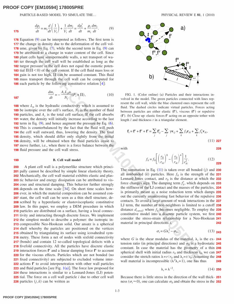
C. Boundary conditions

In fluid mechanics, the contact between the fluid and theboundary is often modeled by no-slip boundary conditions.In SPH, this is accomplished by a direct fluid-boundary cou-pling, assuming ghost particles on the other side of theboundary �31�, or simply assuming that outer SPH particlesrepresent the boundary and superimpose elastic interactions�35�. Both approaches however are not preferable here be-cause the first one can only treat fixed boundaries, while inthe second, the boundaries do not have a distinct physicalidentity. In our implementation, the boundaries are repre-

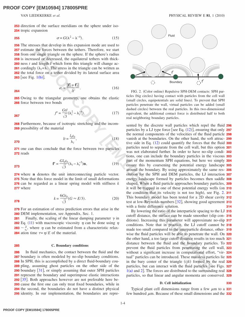
sented by the discrete wall particles which repel the fluidparticles by a LJ type force �see Eq. �12��, ensuring that onlythe normal components of the velocities of the fluid particlevanish at the boundaries. On the other hand, the soft attrac-tive side in Eq. �12� could quantify the forces that the fluidparticles need to separate from the cell wall, but this optionwas not elaborated further. In order to have no-slip condi-tions, one can include the boundary particles in the viscouspart of the momentum SPH equations, but here we simplyensure this by coarsening the potential energy landscapearound the boundary. By using approximately the same res-olution for the SPH and DEM particles, the LJ interactionenergy landscape formed by particles becomes then saddleshaped. When a fluid particle approaches boundary particles,it will be trapped in one of these potential energy wells �onthe condition that its velocity is not too high�, see Fig. 2.This boundary model has been tested for a 2D shear cavitytest at low-Reynolds numbers �32�, showing good agreementwith a finite difference solution.

By lowering the ratio of the interparticle spacing to the LJcutoff distance, the surface can be made smoother �slip con-ditions�. Increasing this parameter will approximate no-slipconditions. Note that in practice, the LJ cutoff cannot bemade too small compared to the interparticle distance, other-wise the fluid particles will be able to penetrate the wall. Onthe other hand, a too large cutoff distance results in too muchdistance between the fluid and the boundary particles. Toprevent the fluid particles from penetrating the cell wall,without a significant increase in computational effort, “vir-tual” particles can be introduced. These massless particles liein the bary center of the triangle �ijk� formed by the realparticles, but can interact with the fluid particles �see Figs.1�a� and 2�. The forces are distributed to the surrounding realparticles, so that linear and angular momenta are conserved.

D. Cell initialization

Typical plant cell dimensions range from a few �m to afew hundred �m. Because of these small dimensions and the

fr

fr

Fluid

Boundary

FIG. 2. �Color online� Repulsive SPH-DEM contacts: SPH par-ticles �big circles� having contact with particles from the cell wall�small circles, equipotentials are solid lines�. To prevent that SPHparticles penetrate the wall, virtual particles can be added �smalldashed circles� between the real particles. In this two-dimensionalequivalent, the additional contact force is distributed half to bothreal neighboring boundary particles.

VAN LIEDEKERKE et al. PHYSICAL REVIEW E 81, 1 �2010�

253254

255

256257258259260261262263

264

265266

267

268269

270

271272

273

274275276277

278

279280281282

283

284

285

286287288289290291292293294295

296297298299300301302303304305306307308309310311312313314315316317318319320321322323324325326327328329

330

331332

1-4

PROOF COPY [EM10594] 178005PRE

PROOF COPY [EM10594] 178005PRE

PROO

F COPY [EM

10594] 178005PRE

fact that biological materials generally show great variability,it is a formidable task to probe mechanical properties ofcells. Moreover, plant cell walls usually have a large elasticmodulus, making it difficult to measure them by AFM oroptical tweezers such as is done on animal cells. Neverthe-less, Wang et al. �36� derived a cell wall Young modulus byconducting plate compression experiments on in vitro tomatocells. In their model, based on the analytical calculations byLardner and Puljara �9�, the cell wall is described by a gen-eralized Hooke’s law using a Young modulus E, the initialthickness of the cell wall, Poisson’s ratio , and the initialstretch ratio as physical parameters, and their model isextended with a cell wall permeability to account for volumeloss during compression. The initial turgor pressure wasmeasured. By monitoring the contact force between the celland the plates and using model parameter fitting, the authorsgenerally found good agreement with the experiment up to20% of compression strain by adopting in their model a cellwall thickness 126 nm, a wall Young modulus of 2.4 GPa,and an initial wall stretch ratio of 1.015. Following the workof Wang and his co-workers, our model considers a sphericalcell with radius 30 �m. The wall shear modulus is estimatedby G=E /3 and hence we use G=0.8 GPa and t0=126 nm inEq. �19�. In this work, we also consider another cell type,which is mechanically softer and has a lower internal pres-sure. This “soft” type mimics an animal cell to the degreethat its wall mechanical properties are in the range of a lipidbilayer. However, it still has the same radius and the New-tonian protoplasm as in the stiff plant cell type. In fact, thiscell may also be regarded as a protoplast of the plant cell.See Table I for all the input parameters.

The cell was initialized with 2562 wall particles �obtainedby icosahedral triangulation, with all bond lengths l0 ap-proximately 2.5 �m� and 3500 fluid particles, initially posi-tioned on a cubic lattice, but delimited by the cell’s radius�see Fig. 3�a��. For the simplicity, all LJ forces were assumedto be repulsive only �dcutof f =r0 in Eq. �12��. We initially setthe wall damping to an arbitrarily small value �pure elasticbehavior� while still retaining stable computations. BothSPH and DEM equations of motion are integrated by a Leap-

frog algorithm. The time step for the SPH equations is de-rived from the CFL criterion, the magnitude of particle ac-celerations, and viscous forces �31,32�. However, this mustbe combined with an additional requirement on the time stepimposed by the stiffness �Eq. �20�� of the wall. In fluid dy-namics, when using an EOS, the compression modulus �plays a crucial role and should be chosen with care. If � islarge, the simulations normally will require a small time stepin order to be stable. If it is chosen too low, the fluid willbehave more like a compressible one. In many SPH simula-tions, the Mach number defines the condition to where thefluid can be regarded as incompressible �33�. Here, this con-dition is further restricted by the flexible boundaries. To en-sure apparent incompressibility of the fluid, it is necessary toset the compression modulus sufficiently high with respect tothe stiffness of the cell wall.

The cell is first simulated to grow artificially fast into afully turgid one by setting a high hydraulic conductivity inEq. �10�. Once the fluid pressure reaches the osmotic poten-tial �38�, the cell is in mechanical equilibrium. During theinflation, the SPH particles are driven outward by the pres-sure, and repelled if they come too close to the cell wall. ByNewton’s third law, this repulsive force will in turn push thecell wall outward. As a consequence, stresses in the cell wallproportional to the fluid pressure will develop �Young-Laplace law�, and the bonds between the boundary particlesbecome slightly extended. On average, we find an initialstretch ratio of the tethers of 1.01, close to what is found byWang and his co-workers. The SPH-DEM coupling has beenbenchmarked with the Young-Laplace condition, and withanalytical solutions for centrosymmetric oscillations, see Ap-pendix, Sec. 2. In Appendix, Sec. 3 we give an idea of thevariations on the results that can be expected due to the dis-cretization.

TABLE I. Model parameters used in the cell model.

ParameterValue

�stiff cell/soft cell� Reference

Cell wall thickness, t 126/5 nm �36�/�37�Cell wall Young modulus, E 2400/20 MPa �36�/�37�Cell radius, R 30 �m �36�Cell wall damping, � 10−10 Nm−1 s Set

Cell fluid viscosity, � 10−3 Pa s–1 Pa s Set

Fluid compression modulus, � 10 MPa Set

Cell turgor pressure, P0 364/0.1 kPa �36�/set

Cell hydraulic conductivity, Lp 10−12 m2 N−1 s �4,36�SPH smoothing length, s 3.2 �m Set

Number fluid particles per cell, Nf 3500 Set

Number wall particles per cell 2562 Set

Cell-plate contact stiffness, kp 1000 Nm−1 Set

FIG. 3. �Color online� Snapshot of �a� an uninflated cell and �b�an inflated cell under compression �X between two plates. The biginner particles represent the cell protoplasm, the small outer par-ticles the cell wall.

PARTICLE-BASED MODEL TO SIMULATE THE… PHYSICAL REVIEW E 81, 1 �2010�

333334335336337338339340341342343344345346347348349350351352353354355356357358359360361362363364365366367368369370371372

373

374

375

376

377

378

379

380

381

382383384385386387388389390391392393394395396397398399400401402403404405406

1-5

PROOF COPY [EM10594] 178005PRE

PROOF COPY [EM10594] 178005PRE

PROO

F COPY [EM

10594] 178005PRE

III. RESULTS AND DISCUSSION

A. Quasistatic compression

Following the in vitro experiment conducted in �36�, thestiff cell is simulated to be compressed between two flatplates. This is achieved by introducing two virtual horizontalplanes with one kept at its position while the other one ismoved downward by a distance �X �see Fig. 3�b��. If thewall particles geometrically overlap this boundary by �, theyare repelled by a force f i=−kp�i. The displacement rate was0.002 ms−1, sufficiently low to exclude inertial effects. Thetotal force acting on the plate by the particles i is obtained by

Fplate = �i

− kp�i, �21�

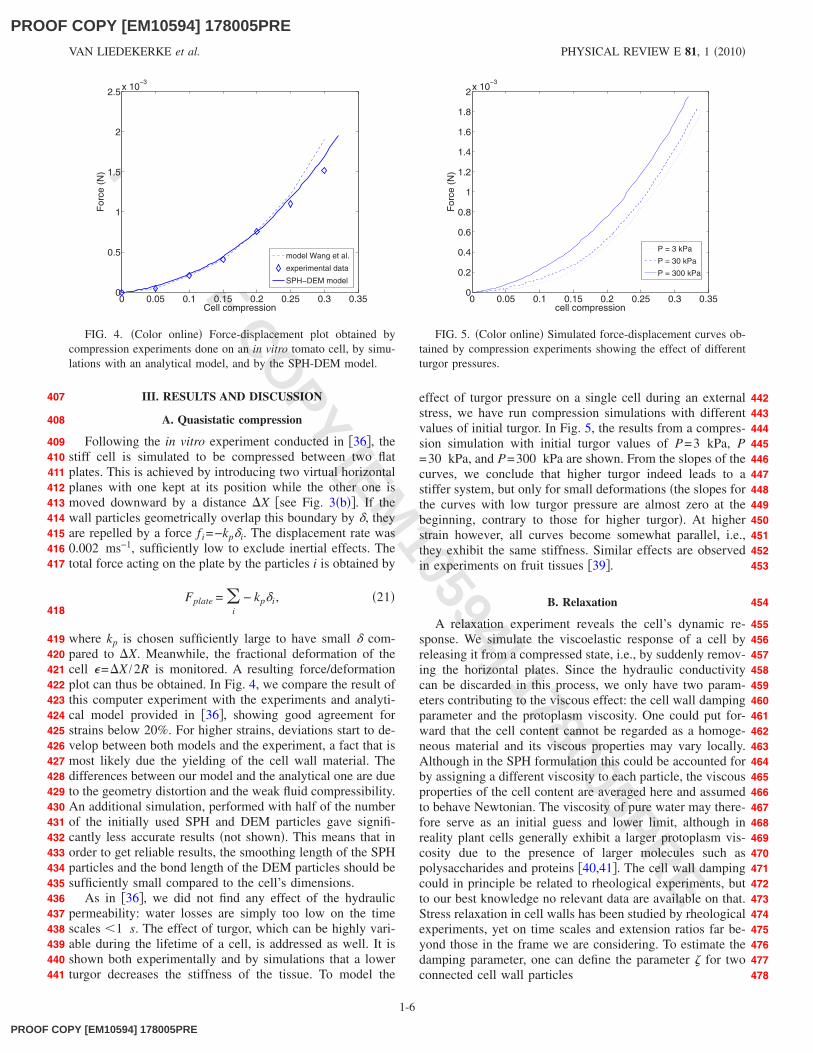
where kp is chosen sufficiently large to have small � com-pared to �X. Meanwhile, the fractional deformation of thecell �=�X /2R is monitored. A resulting force/deformationplot can thus be obtained. In Fig. 4, we compare the result ofthis computer experiment with the experiments and analyti-cal model provided in �36�, showing good agreement forstrains below 20%. For higher strains, deviations start to de-velop between both models and the experiment, a fact that ismost likely due the yielding of the cell wall material. Thedifferences between our model and the analytical one are dueto the geometry distortion and the weak fluid compressibility.An additional simulation, performed with half of the numberof the initially used SPH and DEM particles gave signifi-cantly less accurate results �not shown�. This means that inorder to get reliable results, the smoothing length of the SPHparticles and the bond length of the DEM particles should besufficiently small compared to the cell’s dimensions.

As in �36�, we did not find any effect of the hydraulicpermeability: water losses are simply too low on the timescales �1 s. The effect of turgor, which can be highly vari-able during the lifetime of a cell, is addressed as well. It isshown both experimentally and by simulations that a lowerturgor decreases the stiffness of the tissue. To model the

effect of turgor pressure on a single cell during an externalstress, we have run compression simulations with differentvalues of initial turgor. In Fig. 5, the results from a compres-sion simulation with initial turgor values of P=3 kPa, P=30 kPa, and P=300 kPa are shown. From the slopes of thecurves, we conclude that higher turgor indeed leads to astiffer system, but only for small deformations �the slopes forthe curves with low turgor pressure are almost zero at thebeginning, contrary to those for higher turgor�. At higherstrain however, all curves become somewhat parallel, i.e.,they exhibit the same stiffness. Similar effects are observedin experiments on fruit tissues �39�.

B. Relaxation

A relaxation experiment reveals the cell’s dynamic re-sponse. We simulate the viscoelastic response of a cell byreleasing it from a compressed state, i.e., by suddenly remov-ing the horizontal plates. Since the hydraulic conductivitycan be discarded in this process, we only have two param-eters contributing to the viscous effect: the cell wall dampingparameter and the protoplasm viscosity. One could put for-ward that the cell content cannot be regarded as a homoge-neous material and its viscous properties may vary locally.Although in the SPH formulation this could be accounted forby assigning a different viscosity to each particle, the viscousproperties of the cell content are averaged here and assumedto behave Newtonian. The viscosity of pure water may there-fore serve as an initial guess and lower limit, although inreality plant cells generally exhibit a larger protoplasm vis-cosity due to the presence of larger molecules such aspolysaccharides and proteins �40,41�. The cell wall dampingcould in principle be related to rheological experiments, butto our best knowledge no relevant data are available on that.Stress relaxation in cell walls has been studied by rheologicalexperiments, yet on time scales and extension ratios far be-yond those in the frame we are considering. To estimate thedamping parameter, one can define the parameter � for twoconnected cell wall particles

0 0.05 0.1 0.15 0.2 0.25 0.3 0.350

0.5

1

1.5

2

2.5x 10−3

Cell compression

For

ce(N

)

model Wang et al.

experimental data

SPH−DEM model

FIG. 4. �Color online� Force-displacement plot obtained bycompression experiments done on an in vitro tomato cell, by simu-lations with an analytical model, and by the SPH-DEM model.

0 0.05 0.1 0.15 0.2 0.25 0.3 0.350

0.2

0.4

0.6

0.8

1

1.2

1.4

1.6

1.8

2x 10−3

cell compression

For

ce(N

)

P = 3 kPa

P = 30 kPa

P = 300 kPa

FIG. 5. �Color online� Simulated force-displacement curves ob-tained by compression experiments showing the effect of differentturgor pressures.

VAN LIEDEKERKE et al. PHYSICAL REVIEW E 81, 1 �2010�

407

408

409410411412413414415416417

418

419420421422423424425426427428429430431432433434435436437438439440441

442443444445446447448449450451452453

454

455456457458459460461462463464465466467468469470471472473474475476477478

1-6

PROOF COPY [EM10594] 178005PRE

PROOF COPY [EM10594] 178005PRE

PROO

F COPY [EM

10594] 178005PRE� =

�

�2km, �22�

where k=6Gt0

�3is the stiffness and m is the cell wall particle

mass. The absence of viscous effects is approached if ��1,while the wall material reacts as an overdamped system if��1.

To monitor the relaxation, we compute the equatorialforce Feq for a hemisphere,

Feq = �i

�j

fij , �23�

where fij is the internal force acting on a particle i from theneighboring particles j, and the summation is over all theparticles that lie on this hemisphere �see Appendix, Sec. 2,Fig. 15�. In Fig. 6�a�, this force is plotted as a function oftime for the stiff cell type with a protoplasm viscosity range�1 mPa s–1 Pa s�, assuming a purely elastic cell wall. Ad-ditionally we also show the model results for a slightly over-damped wall material ��=1.1�. The simulations reveal thatthe cell, once released, oscillates several times with a periodless than 1 �s and thus may be regarded as a viscoelasticsolid. The oscillations are damped by both the cell fluid vis-cosity and cell wall damping and the fluid viscosity seems tohave the major influence on this. Interestingly, the stiff cellbehaves as an overdamped system if the cell fluid viscosityexceeds approximately 0.5 Pa s. Note that the response isfast and different from that of animal cells, which behavemore fluidlike. For the soft cell, the equatorial forces in therelaxation experiments are depicted in Fig. 6�b�, showingthat this cell reacts much slower than the stiff type, and ex-hibits weaker oscillations. The relaxation times are 30 �sfor the lowest fluid viscosity, and 5 ms for the highest �thecell wall was assumed to be elastic�. We note that these re-laxation times are still below these observed in animal cells,which are typically around 1 s �17,42�. The cause for thisdiscrepancy is most likely due to the nature of the proto-plasm of these cells, which is a complex fluid and where, incontrast to the plant cell type, a dense cytoskeleton plays adominant role �37,42�.

C. Impact

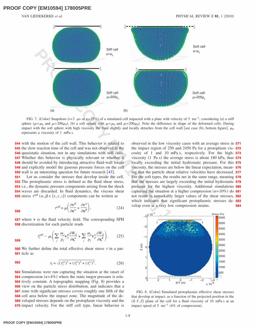
The situation during impact is different to the one of qua-sistatic compression because inertia and viscous effects can-not be ignored. Impacting a cell causes additional stresscomponents on both the cell fluid and cell wall. Here, weconcentrate on the protoplasmic stresses and the forces thatare transmitted by the whole cell. To this end, we start fromthe same simulation setup as in Sec. III A, but with a loadingrate of 5 ms−1. This velocity is well below the Mach numberimposed by the compressibility modulus, thus ensuring theapparent incompressibility of the protoplasm during impact.We look at the two different cell types. Figure 7 providessnapshots of the two cell types at �=25% when impacted.The shape of the cells changes as a shock wave travelsthrough them. The resulting deformation depends on the vis-cosity, with a stronger effect in the soft cell, while the stifftype tends to deform more symmetrically �compare Fig. 7�a�

with Fig. 7�b��. We note the link with the relaxation experi-ments: the impact duration takes only about 3 �s and coversthe relaxation time of the stiff cell. Contrary, it is muchsmaller than the relaxation time of the soft cell, and hencethe latter is unable to follow the deformation.

Generally, we find that the lower the fluid viscosity, thehigher the cell shape deforms during impact. This clearlyvisible in Fig. 7�b� for the soft cell type, which behaves morefluidlike as a whole. We visually observe that in the latter thefluid slightly and locally �in the region of the impacting ob-ject� detaches from the cell wall in case of a high protoplasmviscosity �Fig. 7�b�, bottom�, as it seems unable to keep up

0 1 2 3 4 5x 10

−6

0.8

0.9

1

1.1

1.2

1.3

1.4

1.5

1.6

1.7

1.8x 10−3

time (s)

For

ce(N

)

µ/µ0=1

µ/µ0=10

µ/µ0=100

µ/µ0=1000

γ/γ0=10E5

0 1 2 3 4x 10

−4

2.2

2.4

2.6

2.8

3

3.2

3.4

3.6

3.8

4

x 10−7

time (s)

For

ce(N

)

µ/µ0=1

µ/µ0=10

µ/µ0=100

µ/µ0=200

(b)

(a)

FIG. 6. �Color online� Relaxation experiment, showing the evo-lution of the equatorial force when releasing the cell from a com-pressed state, simulated for a protoplasm viscosity range of1 mPa s–1 Pa s. �0 represents a viscosity of 1 mPa s. �a� Stiffcell type: the cell relaxes in about 1 �s in all cases and furtheroscillates except for the highest fluid viscosity �assuming a low-cellwall damping, ��1�. The response for a highly damped ��=1.1�cell wall material is also given �� is five orders of magnitude largerthan the low damped: �0=10−10 Nm s−1, and �=�0�. �b� The softcell relaxes in 30 �s for a low fluid viscosity. Larger valuesstrongly increase the relaxation time. The transition to an over-damped system occurs for a fluid viscosity of approximately10 mPa s.

PARTICLE-BASED MODEL TO SIMULATE THE… PHYSICAL REVIEW E 81, 1 �2010�

479

480

481482483484485

486

487488489490491492493494495496497498499500501502503504505506507508509510511512513514

515

516517518519520521522523524525526527528529530531

532533534535536537538539540541542543

1-7

PROOF COPY [EM10594] 178005PRE

PROOF COPY [EM10594] 178005PRE

PROO

F COPY [EM

10594] 178005PRE

with the motion of the cell wall. This behavior is related tothe slow reaction time of the cell and was not observed in thequasistatic situation, nor in any simulations with stiff cells.Whether this behavior is physically relevant or whether itshould be avoided by introducing attractive fluid-wall forcesand explicitly model the gaseous pressure forces on the cellwall is an interesting question for future research �43�.

Let us consider the stresses that develop inside the cell.The protoplasmic stress is defined as the fluid shear stress,i.e., the dynamic pressure components arising from the shockwaves are discarded. In fluid dynamics, the viscous shearstress ��� �� ,�� �x ,y ,z�� components can be written as

��� = �� �v�

�x� +�v�

�x�� , �24�

where v is the fluid velocity field. The corresponding SPHdiscretization for each particle reads

�i�� � �i��

j

mj

� jv ji

� �Wij

�xi� + �

j

mj

� jv ji

� �Wij

�xi� � . �25�

We further define the total effective shear stress � in a par-ticle as

�i = ���ixy�2 + ��i

xz�2 + ��iyz�2. �26�

Simulations were run capturing the situation at the onset ofcompression ��=4%� where the static turgor pressure is rela-tively constant. A topographic mapping �Fig. 8� provides aview on the particle stress distribution, and indicates that azone with significant stresses covers roughly one fifth of thecell area below the impact zone. The magnitude of the de-veloped stresses depends on the protoplasm viscosity and theimpact velocity. For the stiff cell type, linear behavior is

observed in the low viscosity cases with an average stress inthe impact region of 250 and 2450 Pa for a protoplasm vis-cosity of 1 and 10 mPa s, respectively. For the high-viscosity �1 Pa s� the average stress is about 180 kPa, thuslocally exceeding the initial hydrostatic pressure. For thisviscosity, the stresses are below the linear expectation, mean-ing that the particle shear relative velocities have decreased.For the soft types, the results are in the same range, meaningthat the stresses are largely exceeding the initial hydrostaticpressure for the highest viscosity. Additional simulationscapturing the situation at a higher compression ��=10%� donot result in remarkably larger values of the shear stresses,which indicates that significant protoplasmic stresses de-velop even at a very low compression strains.

(b)(a)

FIG. 7. �Color� Snapshots �t=3 �s or �=25%� of a simulated cell impacted with a plate with velocity of 5 ms−1, considering �a� a stiffsphere ��=�0 and �=200�0�, �b� a soft sphere with �=�0 and �=200�0�. Note the difference in shape of the deformed cells. Duringimpact with the soft sphere with high viscosity the fluid slightly and locally detaches from the cell wall �see case �b�, bottom figure�. �0

represents a viscosity of 1 mPa s.

X/Y (m)

Z(m

)

−3−2−10123x 10

−5

−3

−2

−1

0

1

2

3

x 10−5

500

1000

1500

2000

2500

3000

3500

4000

4500

5000

5500Stress (Pa)

FIG. 8. �Color� Simulated protoplasmic effective shear stressesthat develop at impact, as a function of the projected position in the�X-Y ,Z� plane of the cell for a fluid viscosity of 10 mPa s at animpact speed of 5 ms−1 �4% of compression�.

VAN LIEDEKERKE et al. PHYSICAL REVIEW E 81, 1 �2010�

544545546547548549550551552553554555

556

557558

559

560561

562

563564565566567568569570

571572573574575576577578579580581582583584

1-8

PROOF COPY [EM10594] 178005PRE

PROOF COPY [EM10594] 178005PRE

PROO

F COPY [EM

10594] 178005PRE

The transmitted force �Eq. �21�� is defined as the forcethat is measured on one side of a cell with an impact regionon the opposite side. Figures 9 and 10 show the transmittedforces as a function of compression strain on the oppositecell side for different cell protoplasm viscosities. With bothcell types, it can be clearly seen that an impact situation isquite different from the quasistatic case. Because of the in-ertia, a lag phase exists between this perturbation and thetransmitted force. However, once this phase is past the forcesbuild up quickly and exceed those in the quasistatic case. Forthe stiff cell, this effect remains quite modest for a viscosityup to 0.1 Pa s, but becomes strongly manifested for a vis-cosity of 1 Pa s, see Fig. 9. In the latter case the lag phase isshorter and hence one could state that the cell behaves morerigid �visible by comparing the top and bottom pictures inFig. 7�a�� whereby the momentum is merely transferreddownward by pressure forces and less toward the transverse

sides of the cell �which introduces shear�. In the soft celltype, the viscous forces play a much larger role than thepressure forces, as the force transmission builds up relativelyfast at a lower viscosity, see Fig. 10.

These simulations can provide estimations of how muchstress the vital parts in a cell will bear on impact, a subjectwhere little research has been conducted on so far. Moreaccurate and local results can be obtained using a finer par-ticle discretization, i.e., a lower smoothing length comparedto the cell’s dimensions. On the other hand, such a refine-ment should go along with capturing more detail of the cel-lular content, by identifying particle clusters with certainsubstructures in the cell. Although this approach is wellsuited for these kind of problems, such additional work re-mains out of the scope of this paper.

D. Failure of the cell

The causes for the failure of a thin fluid-filled shell caneither be internal �e.g., because of an excessive pressure� orexternal �e.g., impact with another object�. Microscopically,the failure of materials originates at local weaknesses or de-fects in the material from where the fracture propagates fur-ther on. The modeling of cracks and their propagation inmaterials is an involved task whereby one could rely on mul-tiscaling approaches. Nevertheless, DEM models employedto simulate the breakup of shells have been able to reproducethe mass fragmental distribution in experiments after impactor explosion �44�. As in the latter, we implement a failurecriterion by assuming a threshold for the local strains be-tween two neighboring particles. Our model thus can onlycapture crack propagation with limited detail, but it has theadvantage that fluid interaction is taken into account in aconsistent way, allowing to make quantitative predictionsabout the behavior of a cell during and after failure. Thiscould be of particular interest when one focuses on the cellaggregates, where the mechanics is not only determined by asingle cell but also depends on interactions with neighboringcells.

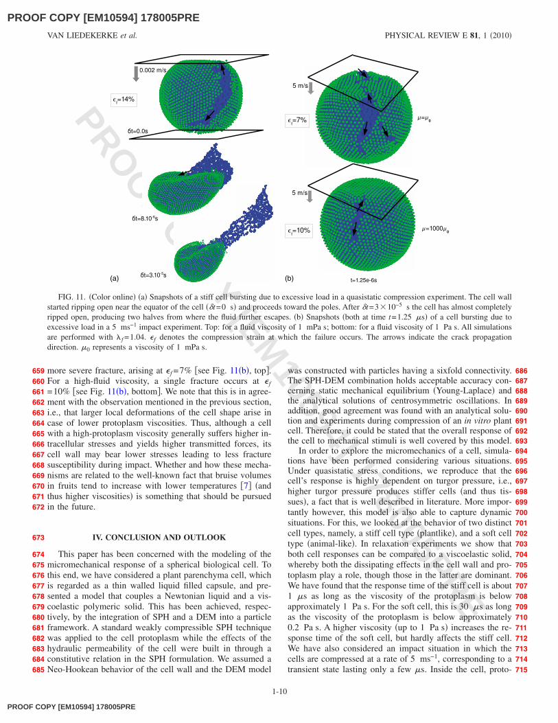
We consider a stiff cell type and assume that a tether onthe membrane fails when its stretch ratio exceeds a criticalvalue f. Since from a material science viewpoint a greatbiological variability can be expected we shall not focus onthe absolute values of this critical extension. A simulationconsidering quasistatic compression was run with arbitrarily f =1.04. This corresponds to a cell compression strain � f=14%, the point from where the cell starts to fail �see Fig.11�a��. A main fracture originates near the equator and pro-ceeds toward the poles, where it stops �this process takes lessthan 0.5 �s�. This can indeed be expected as the largest wallstresses will be those in the directions parallel to the equator.As a result of the crack, a jet of fluid escapes from the twopartially attached halves �the particle speeds in this jet arearound 3 ms−1� �45�. The behavior during impact showsquite a different picture. Due to the asymmetry arising fromthe inertial effects, the fracture originates in the region of theimpacting object where the wall is deformed the most, andoccurs faster in terms of compression strain. This effect isstronger for a low fluid viscosity, where the cell wall suffers

0 0.005 0.01 0.015 0.02 0.025 0.03 0.0350

0.5

1

1.5

2

2.5

3

3.5x 10−3

compression strain

For

ce(N

)

quasi−static

µ/µ0=1

µ/µ0=10

µ/µ0=100

µ/µ0=1000

FIG. 9. �Color online� Transmitted force by the stiff cell at im-pact �5 ms−1� as a function of the compression strain on the oppo-site cell side for different protoplasm viscosities. The quasistaticforce is also depicted. �0 represents a viscosity of 1 mPa s.

0 0.05 0.1 0.15 0.2 0.25 0.30

0.1

0.2

0.3

0.4

0.5

0.6

0.7

0.8

0.9

1x 10−5

For

ce(N

)

compression strain

quasi−static

µ=µ0

µ=10µ0

µ=100µ0

µ=200µ0

FIG. 10. �Color online� Transmitted force by the soft cell atimpact �5 ms−1� as a function of the compression strain on theopposite cell side for different protoplasm viscosities. The quasi-static force is also depicted. �0 represents a viscosity of 1 mPa s.

PARTICLE-BASED MODEL TO SIMULATE THE… PHYSICAL REVIEW E 81, 1 �2010�

585586587588589590591592593594595596597598599600601

602603604605606607608609610611612613614615616

617

618619620621622623624625626627628629630631632633634635636637638639640641642643644645646647648649650651652653654655656657658

1-9

PROOF COPY [EM10594] 178005PRE

PROOF COPY [EM10594] 178005PRE

PROO

F COPY [EM

10594] 178005PRE

more severe fracture, arising at � f =7% �see Fig. 11�b�, top�.For a high-fluid viscosity, a single fracture occurs at � f=10% �see Fig. 11�b�, bottom�. We note that this is in agree-ment with the observation mentioned in the previous section,i.e., that larger local deformations of the cell shape arise incase of lower protoplasm viscosities. Thus, although a cellwith a high-protoplasm viscosity generally suffers higher in-tracellular stresses and yields higher transmitted forces, itscell wall may bear lower stresses leading to less fracturesusceptibility during impact. Whether and how these mecha-nisms are related to the well-known fact that bruise volumesin fruits tend to increase with lower temperatures �7� �andthus higher viscosities� is something that should be pursuedin the future.

IV. CONCLUSION AND OUTLOOK

This paper has been concerned with the modeling of themicromechanical response of a spherical biological cell. Tothis end, we have considered a plant parenchyma cell, whichis regarded as a thin walled liquid filled capsule, and pre-sented a model that couples a Newtonian liquid and a vis-coelastic polymeric solid. This has been achieved, respec-tively, by the integration of SPH and a DEM into a particleframework. A standard weakly compressible SPH techniquewas applied to the cell protoplasm while the effects of thehydraulic permeability of the cell were built in through aconstitutive relation in the SPH formulation. We assumed aNeo-Hookean behavior of the cell wall and the DEM model

was constructed with particles having a sixfold connectivity.The SPH-DEM combination holds acceptable accuracy con-cerning static mechanical equilibrium �Young-Laplace� andthe analytical solutions of centrosymmetric oscillations. Inaddition, good agreement was found with an analytical solu-tion and experiments during compression of an in vitro plantcell. Therefore, it could be stated that the overall response ofthe cell to mechanical stimuli is well covered by this model.

In order to explore the micromechanics of a cell, simula-tions have been performed considering various situations.Under quasistatic stress conditions, we reproduce that thecell’s response is highly dependent on turgor pressure, i.e.,higher turgor pressure produces stiffer cells �and thus tis-sues�, a fact that is well described in literature. More impor-tantly however, this model is also able to capture dynamicsituations. For this, we looked at the behavior of two distinctcell types, namely, a stiff cell type �plantlike�, and a soft celltype �animal-like�. In relaxation experiments we show thatboth cell responses can be compared to a viscoelastic solid,whereby both the dissipating effects in the cell wall and pro-toplasm play a role, though those in the latter are dominant.We have found that the response time of the stiff cell is about1 �s as long as the viscosity of the protoplasm is belowapproximately 1 Pa s. For the soft cell, this is 30 �s as longas the viscosity of the protoplasm is below approximately0.2 Pa s. A higher viscosity �up to 1 Pa s� increases the re-sponse time of the soft cell, but hardly affects the stiff cell.We have also considered an impact situation in which thecells are compressed at a rate of 5 ms−1, corresponding to atransient state lasting only a few �s. Inside the cell, proto-

(b)(a)

FIG. 11. �Color online� �a� Snapshots of a stiff cell bursting due to excessive load in a quasistatic compression experiment. The cell wallstarted ripping open near the equator of the cell ��t=0 s� and proceeds toward the poles. After �t=3�10−5 s the cell has almost completelyripped open, producing two halves from where the fluid further escapes. �b� Snapshots �both at time t=1.25 �s� of a cell bursting due toexcessive load in a 5 ms−1 impact experiment. Top: for a fluid viscosity of 1 mPa s; bottom: for a fluid viscosity of 1 Pa s. All simulationsare performed with f =1.04. � f denotes the compression strain at which the failure occurs. The arrows indicate the crack propagationdirection. �0 represents a viscosity of 1 mPa s.

VAN LIEDEKERKE et al. PHYSICAL REVIEW E 81, 1 �2010�

659660661662663664665666667668669670671672

673

674675676677678679680681682683684685

686687688689690691692693694695696697698699700701702703704705706707708709710711712713714715

1-10

PROOF COPY [EM10594] 178005PRE

PROOF COPY [EM10594] 178005PRE

PROO

F COPY [EM

10594] 178005PREplasmic shear stresses develop in the impact zone, and theseare linearly related to the viscosity for low-viscosity values,but become lower than linear as the viscosity increases. Thesimulations further show that the force transmission throughthe cell at impact is very different from that of a low loadingrate. Due to inertial effects, the force transmitted by the cellis lagged compared to the perturbation, but then rises morequickly. Higher protoplasm viscosities decrease this lag andyield a higher transmitted force, making the overall responsemore rigid. Again, we notice a distinct behavior regardingthe cell type. The stiff cell seems to be able to follow theperturbation, but the soft cell does not: it deforms more andis more susceptible to the protoplasm viscosity.

The strength and failure of shells enclosing a gas or liquidis an important issue in engineering and even daily life, andrelates also to microscopic scales, as cells build up to tissue.By introducing a critical strain in a bond between two par-ticles, we have shown that the dynamics of cell failure can bemodeled quantitatively. Under quasistatic loading, fractureoriginates at the equator of the cell and propagates furthertoward the poles. This is in contrast with the impact loadingwhere the fracture originates near the impact region, is af-fected by the protoplasm viscosity, and occurs at a relativelylow compression strain.

As a conclusion, we have shown that this combination oftwo particle methods generates possibilities for simulatingcellular mechanics. A strong advantage is the adaptivity ofthe method, which should make a cell centered approachpossible, a task that will be harder to implement in a FEMapproach �24�. Adding more particles to the system can re-sult in two different approaches. In fine-grained models of acell, one could capture more subcellular detail, which is es-sentially important for a better understanding of the relationbetween cellular micromechanics and biological processes.For example, particles or particle clusters can be viewed ascell organelles or the cytoskeleton �26,35�. From anotherviewpoint, by integrating cells to an aggregate, and introducecell-cell adhesion, yielding, and debonding mechanisms, aresulting multicellular system can provide answers to prob-lems related to the tissue scale �6�. Considering the benefitsof SPH, one could particularly investigate the micromechani-cal cellular stresses in tissues that develop during short andviolent situations.

ACKNOWLEDGMENTS

This research is conducted utilizing high-performancecomputational resources provided by the University of Leu-ven, http://ludit.kuleuven.be/hpc. The authors would like tothank Onderzoekstoelage �OT, KULeuven� and the ResearchFoundation-Flanders �FWO-Vlaanderen� for financial sup-port. We are also grateful to Johan Meyers �KULeuven�.

APPENDIX: ERROR ESTIMATIONS

1. Accuracy of the triangulated particle cellwall model during deformations

A triangulated particle discretization with equilateral teth-ers predicts the stress exactly under isotropic stretch, which

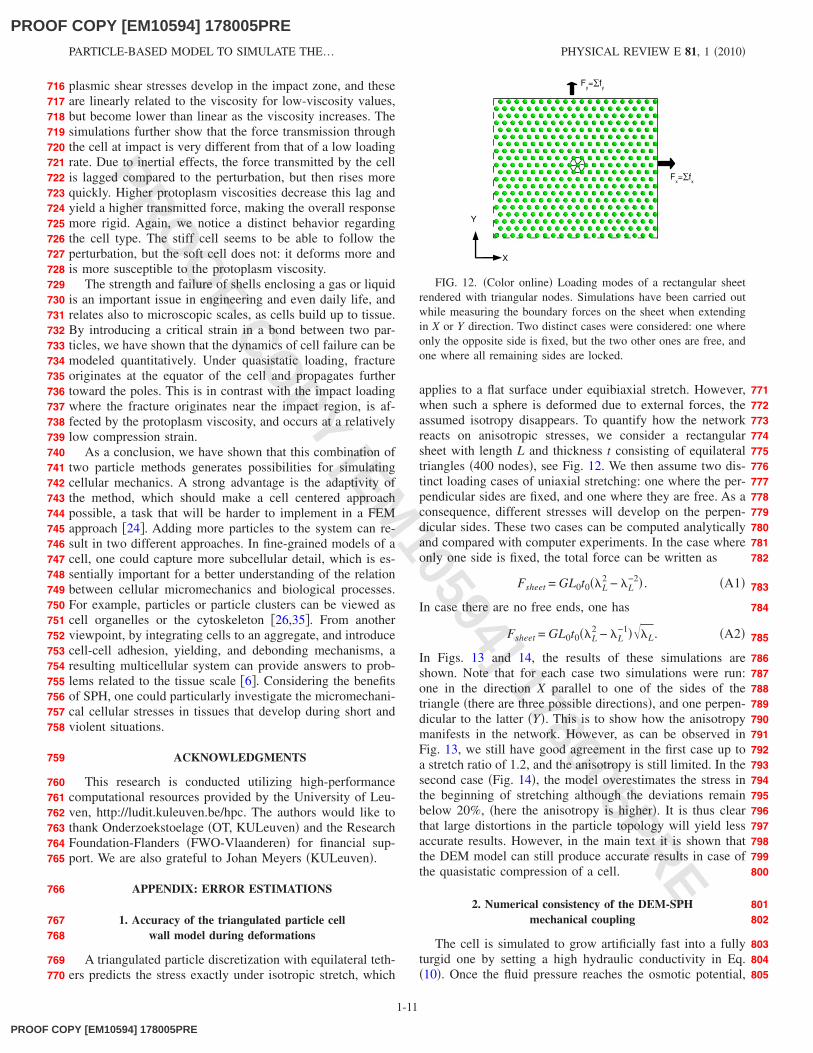
applies to a flat surface under equibiaxial stretch. However,when such a sphere is deformed due to external forces, theassumed isotropy disappears. To quantify how the networkreacts on anisotropic stresses, we consider a rectangularsheet with length L and thickness t consisting of equilateraltriangles �400 nodes�, see Fig. 12. We then assume two dis-tinct loading cases of uniaxial stretching: one where the per-pendicular sides are fixed, and one where they are free. As aconsequence, different stresses will develop on the perpen-dicular sides. These two cases can be computed analyticallyand compared with computer experiments. In the case whereonly one side is fixed, the total force can be written as

Fsheet = GL0t0�L2 − L

−2� . �A1�

In case there are no free ends, one has

Fsheet = GL0t0�L2 − L

−1��L. �A2�

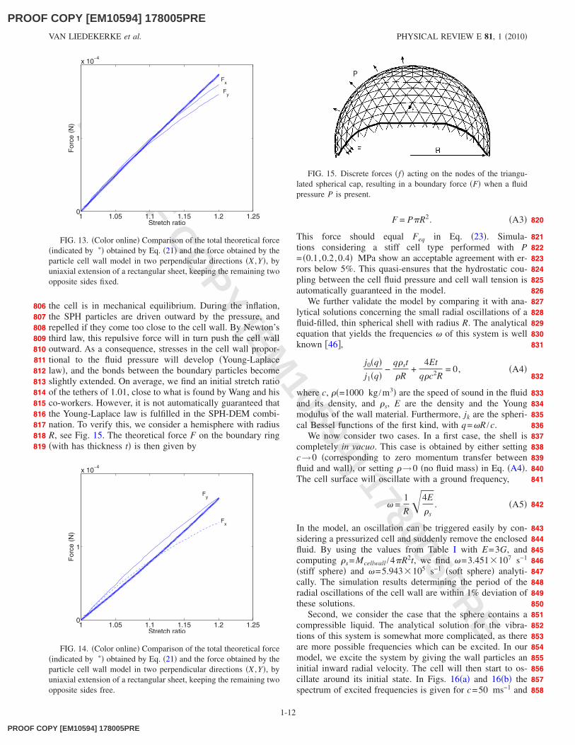
In Figs. 13 and 14, the results of these simulations areshown. Note that for each case two simulations were run:one in the direction X parallel to one of the sides of thetriangle �there are three possible directions�, and one perpen-dicular to the latter �Y�. This is to show how the anisotropymanifests in the network. However, as can be observed inFig. 13, we still have good agreement in the first case up toa stretch ratio of 1.2, and the anisotropy is still limited. In thesecond case �Fig. 14�, the model overestimates the stress inthe beginning of stretching although the deviations remainbelow 20%, �here the anisotropy is higher�. It is thus clearthat large distortions in the particle topology will yield lessaccurate results. However, in the main text it is shown thatthe DEM model can still produce accurate results in case ofthe quasistatic compression of a cell.

2. Numerical consistency of the DEM-SPHmechanical coupling

The cell is simulated to grow artificially fast into a fullyturgid one by setting a high hydraulic conductivity in Eq.�10�. Once the fluid pressure reaches the osmotic potential,

FIG. 12. �Color online� Loading modes of a rectangular sheetrendered with triangular nodes. Simulations have been carried outwhile measuring the boundary forces on the sheet when extendingin X or Y direction. Two distinct cases were considered: one whereonly the opposite side is fixed, but the two other ones are free, andone where all remaining sides are locked.

PARTICLE-BASED MODEL TO SIMULATE THE… PHYSICAL REVIEW E 81, 1 �2010�

716717718719720721722723724725726727728729730731732733734735736737738739740741742743744745746747748749750751752753754755756757758

759

760761762763764765

766

767768

769770

771772773774775776777778779780781782

783

784

785

786787788789790791792793794795796797798799800

801802

803804805

1-11

PROOF COPY [EM10594] 178005PRE

PROOF COPY [EM10594] 178005PRE

PROO

F COPY [EM

10594] 178005PRE

the cell is in mechanical equilibrium. During the inflation,the SPH particles are driven outward by the pressure, andrepelled if they come too close to the cell wall. By Newton’sthird law, this repulsive force will in turn push the cell walloutward. As a consequence, stresses in the cell wall propor-tional to the fluid pressure will develop �Young-Laplacelaw�, and the bonds between the boundary particles becomeslightly extended. On average, we find an initial stretch ratioof the tethers of 1.01, close to what is found by Wang and hisco-workers. However, it is not automatically guaranteed thatthe Young-Laplace law is fulfilled in the SPH-DEM combi-nation. To verify this, we consider a hemisphere with radiusR, see Fig. 15. The theoretical force F on the boundary ring�with has thickness t� is then given by

F = P�R2. �A3�

This force should equal Feq in Eq. �23�. Simula-tions considering a stiff cell type performed with P= �0.1,0.2,0.4� MPa show an acceptable agreement with er-rors below 5%. This quasi-ensures that the hydrostatic cou-pling between the cell fluid pressure and cell wall tension isautomatically guaranteed in the model.

We further validate the model by comparing it with ana-lytical solutions concerning the small radial oscillations of afluid-filled, thin spherical shell with radius R. The analyticalequation that yields the frequencies � of this system is wellknown �46�,

j0�q�j1�q�

−q�st

�R+

4Et

q�c2R= 0, �A4�

where c, ��=1000 kg /m3� are the speed of sound in the fluidand its density, and �s, E are the density and the Youngmodulus of the wall material. Furthermore, jk are the spheri-cal Bessel functions of the first kind, with q=�R /c.

We now consider two cases. In a first case, the shell iscompletely in vacuo. This case is obtained by either settingc→0 �corresponding to zero momentum transfer betweenfluid and wall�, or setting �→0 �no fluid mass� in Eq. �A4�.The cell surface will oscillate with a ground frequency,

� =1

R�4E

�s. �A5�

In the model, an oscillation can be triggered easily by con-sidering a pressurized cell and suddenly remove the enclosedfluid. By using the values from Table I with E=3G, andcomputing �s=Mcellwall /4�R2t, we find �=3.451�107 s−1

�stiff sphere� and �=5.943�105 s−1 �soft sphere� analyti-cally. The simulation results determining the period of theradial oscillations of the cell wall are within 1% deviation ofthese solutions.

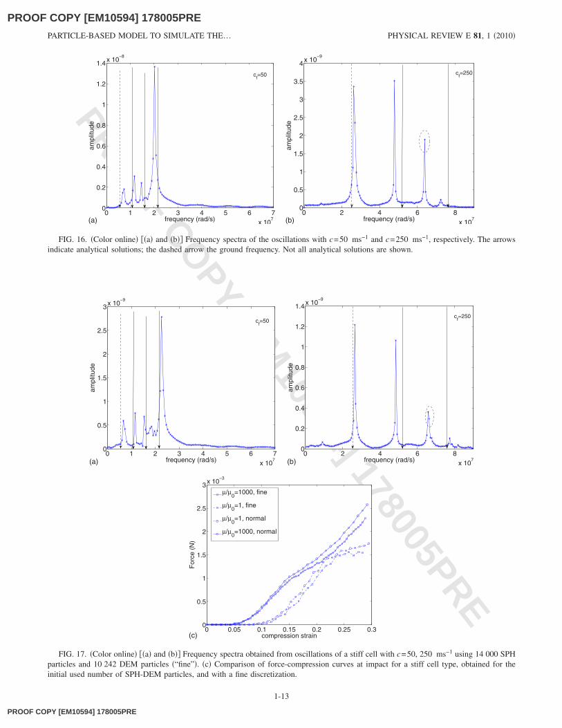
Second, we consider the case that the sphere contains acompressible liquid. The analytical solution for the vibra-tions of this system is somewhat more complicated, as thereare more possible frequencies which can be excited. In ourmodel, we excite the system by giving the wall particles aninitial inward radial velocity. The cell will then start to os-cillate around its initial state. In Figs. 16�a� and 16�b� thespectrum of excited frequencies is given for c=50 ms−1 and

1 1.05 1.1 1.15 1.2 1.250

1

x 10−4

Stretch ratio

For

ce(N

)

Fy

Fx

FIG. 13. �Color online� Comparison of the total theoretical force�indicated by �� obtained by Eq. �21� and the force obtained by theparticle cell wall model in two perpendicular directions �X ,Y�, byuniaxial extension of a rectangular sheet, keeping the remaining twoopposite sides fixed.

1 1.05 1.1 1.15 1.2 1.250

1

x 10−4

Stretch ratio

For

ce(N

)

Fx

Fy

FIG. 14. �Color online� Comparison of the total theoretical force�indicated by �� obtained by Eq. �21� and the force obtained by theparticle cell wall model in two perpendicular directions �X ,Y�, byuniaxial extension of a rectangular sheet, keeping the remaining twoopposite sides free.

FIG. 15. Discrete forces �f� acting on the nodes of the triangu-lated spherical cap, resulting in a boundary force �F� when a fluidpressure P is present.

VAN LIEDEKERKE et al. PHYSICAL REVIEW E 81, 1 �2010�

806807808809810811812813814815816817818819

820

821822823824825826827828829830831

832

833834835836837838839840841

842

843844845846847848849850851852853854855856857858

1-12

PROOF COPY [EM10594] 178005PRE

PROOF COPY [EM10594] 178005PRE

PROO

F COPY [EM

10594] 178005PRE

0 1 2 3 4 5 6 7x 10

7

0

0.2

0.4

0.6

0.8

1

1.2

1.4x 10−8

cf=50

frequency (rad/s)

ampl

itude

0 2 4 6 8x 10

7

0

0.5

1

1.5

2

2.5

3

3.5

4x 10−9

frequency (rad/s)

ampl

itude

cf=250

(b)(a)

FIG. 16. �Color online� ��a� and �b�� Frequency spectra of the oscillations with c=50 ms−1 and c=250 ms−1, respectively. The arrowsindicate analytical solutions; the dashed arrow the ground frequency. Not all analytical solutions are shown.

0 0.05 0.1 0.15 0.2 0.25 0.30

0.5

1

1.5

2

2.5

3x 10−3

compression strain

For

ce(N

)

µ/µ0=1000, fine

µ/µ0=1, fine

µ/µ0=1, normal

µ/µ0=1000, normal

0 1 2 3 4 5 6 7x 10

7

0

0.5

1

1.5

2

2.5

3x 10−9

cf=50

frequency (rad/s)

ampl

itude

0 2 4 6 8x 10

7

0

0.2

0.4

0.6

0.8

1

1.2

1.4x 10−9

frequency (rad/s)

ampl

itude

cf=250

(b)(a)

(c)

FIG. 17. �Color online� ��a� and �b�� Frequency spectra obtained from oscillations of a stiff cell with c=50, 250 ms−1 using 14 000 SPHparticles and 10 242 DEM particles �“fine”�. �c� Comparison of force-compression curves at impact for a stiff cell type, obtained for theinitial used number of SPH-DEM particles, and with a fine discretization.

PARTICLE-BASED MODEL TO SIMULATE THE… PHYSICAL REVIEW E 81, 1 �2010�

1-13

PROOF COPY [EM10594] 178005PRE

PROOF COPY [EM10594] 178005PRE

PROO

F COPY [EM

10594] 178005PREc=250 ms−1, respectively. In addition, the theoretical fre-quencies are also shown �arrows�. The dashed arrows indi-cate ground frequencies. For low c ��50 ms−1�, the frequen-cies are close to each other and a comparison with theanalytical solution is difficult. For higher values of c thecomparison becomes clearer. The model captures the groundmode and at least two higher frequencies reasonably �devia-tions are between 5% and 10%, due to the discretizationerrors and the fluid-boundary coupling�. For the large c �Fig.16�b��, a mode shows up which is not close to any analyticalsolution �indicated by dashed ellipse�. We address this dis-crepancy between model and analytical solution to the influ-ence of the LJ connection between boundary and fluid,which is not accounted for in Eq. �A4�. However, we arguethat in the case of high � �c=265 ms−1 is used in the simu-lations�, the influence of the latter can be minimized becausethe time scale of the dynamics we are considering here �e.g.,

impact, relaxation� is ten times higher, and in addition, theamplitudes of these oscillations are relatively small. The firsttwo frequencies are within 6% deviation from the analyticalsolution.

3. Particle discretization

We have also tested the model for numerical consistencyby performing simulations with four times the number ofSPH-DEM particles. In Figs. 17�a� and 17�b� the frequencyspectrum for the centrosymmetric oscillations in the case ofc=50 ms−1 and c=100 ms−1 are depicted. The results arecomparable with the coarser discretization although showinga slightly better agreement with the analytical solutions. Fur-thermore, it is shown in Fig. 17�c� that for the impact of thecell, the initial and the fine discretization hold an acceptableconsistency.

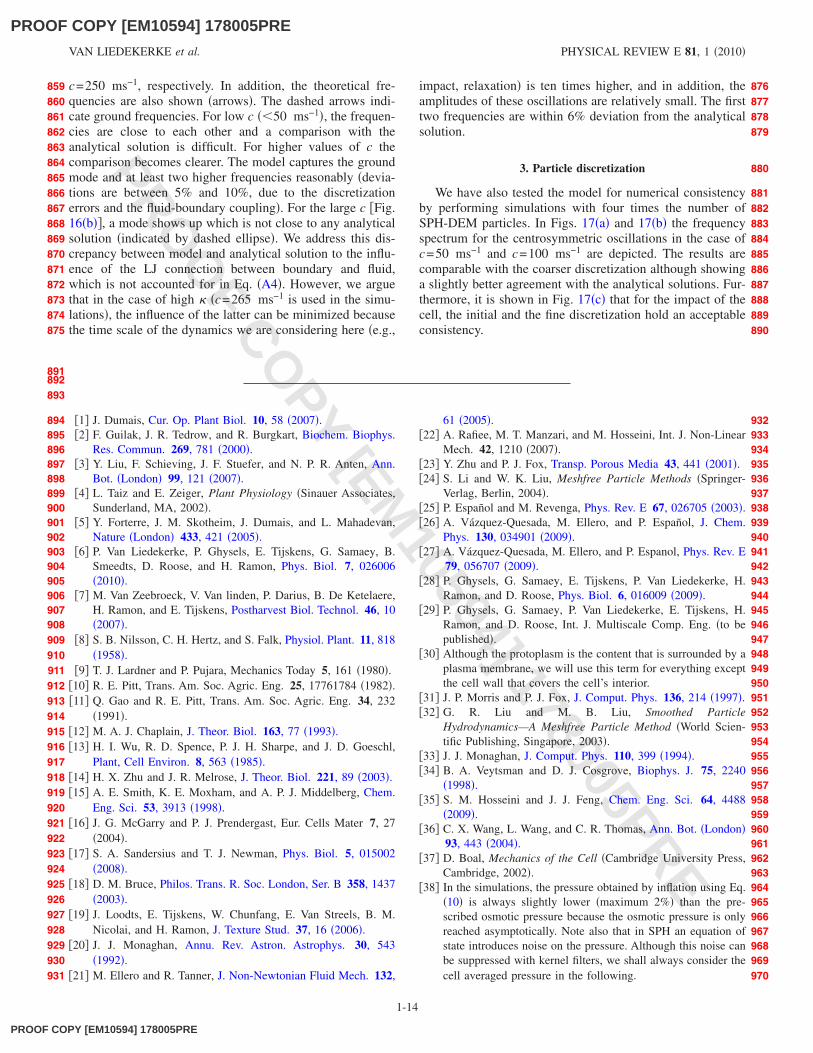
�1� J. Dumais, Cur. Op. Plant Biol. 10, 58 �2007�.�2� F. Guilak, J. R. Tedrow, and R. Burgkart, Biochem. Biophys.

Res. Commun. 269, 781 �2000�.�3� Y. Liu, F. Schieving, J. F. Stuefer, and N. P. R. Anten, Ann.

Bot. �London� 99, 121 �2007�.�4� L. Taiz and E. Zeiger, Plant Physiology �Sinauer Associates,

Sunderland, MA, 2002�.�5� Y. Forterre, J. M. Skotheim, J. Dumais, and L. Mahadevan,

Nature �London� 433, 421 �2005�.�6� P. Van Liedekerke, P. Ghysels, E. Tijskens, G. Samaey, B.

Smeedts, D. Roose, and H. Ramon, Phys. Biol. 7, 026006�2010�.

�7� M. Van Zeebroeck, V. Van linden, P. Darius, B. De Ketelaere,H. Ramon, and E. Tijskens, Postharvest Biol. Technol. 46, 10�2007�.

�8� S. B. Nilsson, C. H. Hertz, and S. Falk, Physiol. Plant. 11, 818�1958�.

�9� T. J. Lardner and P. Pujara, Mechanics Today 5, 161 �1980�.�10� R. E. Pitt, Trans. Am. Soc. Agric. Eng. 25, 17761784 �1982�.�11� Q. Gao and R. E. Pitt, Trans. Am. Soc. Agric. Eng. 34, 232

�1991�.�12� M. A. J. Chaplain, J. Theor. Biol. 163, 77 �1993�.�13� H. I. Wu, R. D. Spence, P. J. H. Sharpe, and J. D. Goeschl,

Plant, Cell Environ. 8, 563 �1985�.�14� H. X. Zhu and J. R. Melrose, J. Theor. Biol. 221, 89 �2003�.�15� A. E. Smith, K. E. Moxham, and A. P. J. Middelberg, Chem.

Eng. Sci. 53, 3913 �1998�.�16� J. G. McGarry and P. J. Prendergast, Eur. Cells Mater 7, 27

�2004�.�17� S. A. Sandersius and T. J. Newman, Phys. Biol. 5, 015002

�2008�.�18� D. M. Bruce, Philos. Trans. R. Soc. London, Ser. B 358, 1437

�2003�.�19� J. Loodts, E. Tijskens, W. Chunfang, E. Van Streels, B. M.

Nicolai, and H. Ramon, J. Texture Stud. 37, 16 �2006�.�20� J. J. Monaghan, Annu. Rev. Astron. Astrophys. 30, 543

�1992�.�21� M. Ellero and R. Tanner, J. Non-Newtonian Fluid Mech. 132,

61 �2005�.�22� A. Rafiee, M. T. Manzari, and M. Hosseini, Int. J. Non-Linear

Mech. 42, 1210 �2007�.�23� Y. Zhu and P. J. Fox, Transp. Porous Media 43, 441 �2001�.�24� S. Li and W. K. Liu, Meshfree Particle Methods �Springer-

Verlag, Berlin, 2004�.�25� P. Español and M. Revenga, Phys. Rev. E 67, 026705 �2003�.�26� A. Vázquez-Quesada, M. Ellero, and P. Español, J. Chem.

Phys. 130, 034901 �2009�.�27� A. Vázquez-Quesada, M. Ellero, and P. Espanol, Phys. Rev. E

79, 056707 �2009�.�28� P. Ghysels, G. Samaey, E. Tijskens, P. Van Liedekerke, H.

Ramon, and D. Roose, Phys. Biol. 6, 016009 �2009�.�29� P. Ghysels, G. Samaey, P. Van Liedekerke, E. Tijskens, H.

Ramon, and D. Roose, Int. J. Multiscale Comp. Eng. �to bepublished�.

�30� Although the protoplasm is the content that is surrounded by aplasma membrane, we will use this term for everything exceptthe cell wall that covers the cell’s interior.

�31� J. P. Morris and P. J. Fox, J. Comput. Phys. 136, 214 �1997�.�32� G. R. Liu and M. B. Liu, Smoothed Particle

Hydrodynamics—A Meshfree Particle Method �World Scien-tific Publishing, Singapore, 2003�.

�33� J. J. Monaghan, J. Comput. Phys. 110, 399 �1994�.�34� B. A. Veytsman and D. J. Cosgrove, Biophys. J. 75, 2240

�1998�.�35� S. M. Hosseini and J. J. Feng, Chem. Eng. Sci. 64, 4488

�2009�.�36� C. X. Wang, L. Wang, and C. R. Thomas, Ann. Bot. �London�

93, 443 �2004�.�37� D. Boal, Mechanics of the Cell �Cambridge University Press,

Cambridge, 2002�.�38� In the simulations, the pressure obtained by inflation using Eq.

�10� is always slightly lower �maximum 2%� than the pre-scribed osmotic pressure because the osmotic pressure is onlyreached asymptotically. Note also that in SPH an equation ofstate introduces noise on the pressure. Although this noise canbe suppressed with kernel filters, we shall always consider thecell averaged pressure in the following.

VAN LIEDEKERKE et al. PHYSICAL REVIEW E 81, 1 �2010�

859860861862863864865866867868869870871872873874875

891892893

894895896897898899900901902903904905906907908909910911912913914915916917918919920921922923924925926927928929930931

876877878879

880

881882883884885886887888889890

932933934935936937938939940941942943944945946947948949950951952953954955956957958959960961962963964965966967968969970

1-14

PROOF COPY [EM10594] 178005PRE

PROOF COPY [EM10594] 178005PRE

PROO

F COPY [EM

10594] 178005PRE�39� M. L. Oey, E. Vanstreels, J. De Baerdemaker, E. Tijskens, H.

Ramon, M. Hertog, and B. M. Nicolai, Postharvest Biol. Tech-nol. 44, 240 �2007�.

�40� F. Fushimi and A. Verkman, J. Cell Biol. 112, 719 �1991�.�41� P. Scherp and K. H. Hasenstein, Am. J. Bot. 94, 1930 �2007�.�42� F. Wottawah, S. Schinkinger, B. Lincoln, R. Ananthakrishnan,

M. Romeyke, J. Guck, and J. Kas, Phys. Rev. Lett. 94, 098103�2005�.

�43� Nevertheless, in plant cells, the protoplast can detach from the

cell wall in plasmolyzed cells �4�, which have lost a part oftheir water content and where the turgor pressure approacheszero.

�44� F. K. Wittel, F. Kun, H. J. Herrmann, and B. H. Kroplin, Phys.Rev. E 71, 016108 �2005�.

�45� Note that protoplasm surface tensions are discarded.�46� P. M. Morse and H. Feshbach, Methods of Theoretical Physics

�McGraw-Hill, New York, 1953�.

PARTICLE-BASED MODEL TO SIMULATE THE… PHYSICAL REVIEW E 81, 1 �2010�

971972973974975976977978979

980

981

982

983

984

985

986

987

1-15

PROOF COPY [EM10594] 178005PRE