J . Fluid Mech. (1987), vol. 185, pp. 447468 Printed in Great Britain

447

On the performance of particle tracking

By JUAN C. A G o f t

AND J. JIMENEZ

School of Aeronautics, Universidad PolitAcnica, 28040 Madrid, Spain

IBM Scientific Centre, Paseo Cwtellana 4, 28046 Madrid, Spain and School of Aeronautics, Universidad PolitBcnice, 28040, Madrid, Spain

(Received 2 September 1986 and in revised form 28 May 1987)

The sources of error associated with the use of particle-tracking techniques in the measurement of velocity and vorticity fields in moderately three-dimensional turbulent flows are analysed. The two dominant sources of error are the visualisation error, resulting from the limited resolution of the optical data acquisition system, and the sampling error, due to limited particle concentration. Their relative importance is discussed.

The performance of the interpolation methods used to translate the measurements from the positions of the particles to an arbitrary point is discussed, and a non- parametric algorithm is given to estimate the errors that arise, using only the available data. The smoothing of the results to produce flow maps of a given statistical significance is also discussed. Finally, the method is validated using simultaneous laser-Doppler velocity measurements.

The system is applied to measurements of the near wake of a circular cylinder. Velocity and vorticity maps are provided which throw light on the process by which the large eddies form and relax to their final equilibrium configurations.

1. Introduction Particle tracking is one of the simplest and most powerful methods of quantitative

flow visualization, and one of the few capable of providing instantaneous maps of magnitudes, such as velocity or vorticity, over extended areas. The technique has been used for a long time, especially in liquids (Prandtl & Tietjens 1934; Werle 1973; Clayton & Massey 1967; Merzkichz 1974; Emrich 1981), and a modern review can be found in Sommerscales (1980). However, the study of the problems associated with the extraction of quantitative information from the experimental output (usually a photographic image) is recent. This is probably due to the lack, before the availability of digital computers, of practical methods for handling the large amount of information provided by the method.

In its modern form, particle tracking involves seeding the flow with particles, which are assumed to follow the fluid, and measuring their movement over a known period of time, either by tracking the particles among different instantaneous pictures, or by measuring the length of their traces on images obtained with a finite exposure. The resulting velocities are associated to some intermediate position between the two end points of the trace, and interpolated to a regular grid or to a

t Present address : Dept. Aeronautics & Astronautics, Stanford University, Stanford, CA 94306, USA.

448 J . C . Agiii and J . Jim4nez

series of contour lines. This part of the data processing usually involves digitization of the pictures, either manually (Imaichi & Ohmi 1983; Utami & Ueno 1984,1987), or automatically (Dimotakis, Debussy BE Koochesfahani 1981 ; Jian & Schmitt 1982), and processing in a computer.

All these steps introduce errors in the final estimation of the velocities. Some of the authors cited above have paid considerable attention to the errors introduced by the visualization technique, but few of them have considered the errors committed during the interpolation process, or the influence of the particle concentration on the maximum resolving power. Also, a validation of the method by correlation with simultaneous measurements by other established means is generally missing.

The experiment described in this paper was undertaken in order to estimate the errors introduced by the particle-tracking method, both in the measuring of two- dimensional velocity and in the estimation of derived quantities such as vorticity. Since this latter step includes a numerical differentiation, it tends to amplify previous errors, and a good error analysis is mandatory.

Our interest was in moderately three-dimensional turbulent flows, and we used the near wake of a circular cylinder as a representative example. It was soon apparent that, in our particular case, an important source of error was the limited sampling resolution provided by the particle concentration, and this aspect is extensively studied below. A problem was that classical sampling theory dealt mostly with regular sampling schemes, and that there were few results available for the random sampling distributions which are characteristic of particle tracking. It was, therefore, necessary to develop some theoretical understanding of the reconstruction techniques that could be used in this case.

This was done by numerical experimentation on simulated sinusoidal velocity fields. We tested several interpolation schemes, choosing finally a modified weighted convolution window. The results presented here apply to that technique. We present both empirical rules for the estimation of the errors of interpolation for a given particle density and for a given power spectrum of the velocity fluctuations, and a non-parametric approximate error estimator for those cases in which those parameters are not known.

Finally, we present some simultaneous laser-Doppler and particle- tracking velocity measurements, that demonstrate both the reliability of the method, within the estimated error bounds, and the approximate correctness of those bounds.

2. Experimental procedure A smooth brass cylinder, 1 cm in diameter, was placed horizontally, normal to the

main flow direction, in a Plexiglas recirculating water tunnel whose test section was 8 cm high and 4 cm wide (figure 1). The tunnel was run at 18 cm/s, giving a Reynolds number, based in the cylinder diameter, a little below 2000, and the wake was studied between 5 and 23 diameters downstream from the cylinder. In this range the wake is turbulent, with significant three-dimensionality extending to the largest scales (Gerrard 1966; Papailiou & Lykoudis 1974).

The free-stream turbulence level was not measured, but was probably high, over 1 %. This was due to the need to remove several blocks of foam, originally used as flow steadiers, to allow for the circulation of the particles. Since the purpose of the experiment was the calibration of the method of measurement, rather than the study of the flow, no effort was made to install alternative turbulence-reduction devices

On the performance of particle tracking 449

FIQURE 1. Experimental &-up for the generation of particle-tracing pictures. The rotating disk acts aa a programmable shutter to produce light pulses, and traces, of any desired shape.

and, as a consequence, the measurements presented here can only be considered indicative for the study of the wake itself.

The particles were fabricated by us from Pliolite (a Styrene-Butadiene resin), and were roughly spherical, with diameters ranging from 70 to 170 pm, and a density of 1.1 g/cms, which is close enough to that of water to avoid significant buoyancy effects (see below).

A narrow sheet of light was placed perpendicular to the cylinder and parallel to the flow direction. Taking a photograph with a long exposure resulted in a collection of streaks that could be considered as projections of the instantaneous velocity vectors onto the plane of the light sheet (figure 2). The camera used was a standard SLR Olimpus OM-1 with a motorized winder, allowing a maximum rate of 2.5 frames pers. Tests performed on the stability of the shutter aperture times were not satisfactory, and it was decided to control the exposure by switching the illumination, with the camera shutter kept open, to bracket the lighting pulse. In our illumination system, a 100 W halogen lamp and a suitable optical system concentrate the light to a point, where a rotating wheel, acting like a light chopper, does the switching. Any desired shape of the light pulse can be achieved by masking appropriately the outer part of the wheel. The emerging cone of light was then converted into a slowly convergent sheet, which was finally masked on the top wall of the tunnel to a rectangular shape, 20 cm long and 2 mm wide.

The ability to shape the light pulse allowed us to solve a problem that is frequently encountered in particle tracking experiments ; if the flow is three-dimensional, it is not easy to distinguish between traces that are limited by the finite light pulse, and those that simply cross the light sheet and correspond to an incomplete time interval.

450 J . C. Agui and J . JimLnez

FIQURE 2. Particle-tracing photograph of a section of the wake. Flow is from left to right and spans approximately from 1 1 to 22 diameters downstream of the cylinder. Note the dot at each end of each trace that serves to ensure its integrity.

We shaped our lighting pulse so that each complete trace was formed by an initial dot, a long period and a final dot. Whenever the complete pattern was seen in the picture, the central part of the streak could be safely used for measurements. Incomplete traces were rejected. Typical time intervals were 10 ms for the central part of the pulse and 153 ms for each wheel rotation.

Synchronization was achieved electronically. An optical switch, placed on the rotating wheel, was closed at every turn. A counter, preset to any desired number of turns, allowed for skipping some of the rotations of the wheel, and its zero fired the camera. The distance on the wheel between the triggering mark and the transparent section was used to account for the delay (100 ms) between the firing pulse and the shutter opening.

Digitization of the traces was done manually on a digitizing tablet, using high- contrast, 18 x 24 cm, prints of the visualization pictures. The coordinates of the two end points of every valid streak were fed into the computer and the resulting velocity was associated to the midpoint of the trace. Traces lacking any of the two ‘safety’ dots were not used in the measurements. Since there was clearly no flow reversal in this part of the wake, there was never any doubt in assigning a direction of motion to the particles. If that had been the case, the ambiguity could have been easily removed by adding one more marking dot to one of the end points of the illumination pulse. The number of traces present in a single picture ranged from 1000 to 1500.

On the performance of particle tracking 45 1

3. Visualization errors We deal in this section with those errors that are intrinsic to the visualization

procedure, and that result in an incorrect velocity being associated to a given particle trace. The interpolation error, that comes from the attempt to translate the velocities, known at the traces, to other points in the flow, is discussed in the next section. Both sources of error are largely independent, and may be treated separately.

3.1. Picture digitimtion The precision with which the length of the particle traces can be measured is limited by the resolution of the photographic film and by the accuracy of the digitization. In our case, the film was Tri-X which, when pushed to high sensitivity, has an approximate resolving power of 60 lines/mm, or 15 pm. When the 35 mm negative is enlarged to a 18 x 24 cm print, this corresponds to a maximum resolution of 0.1 mm, which was also the resolution of our digitizing tablet.

We ran tests on the repeatability of manual digitization by comparing successive digitizations of a single, sharp, point by the same operator, and found an r.m.8. deviation of 0.2 mm, which is probably not limited by the accuracy of the tablet, but intrinsic to the hand positioning of the cursor. If it is assumed that this is the accuracy with which each end point is known, and that the errors on both ends are uncorrelated, and since only the projection of the error on the direction of the trace is important, the expected r.m.s. error of the estimation of the length of the trace is again 0.2 mm, measured on the print, which corresponds to 0.1 mm on the flow. Since the average trace length, at the flow, is 2 mm, this results in a relative error Of 5%.

Note that automatic digitization could have decreased this error by a factor of two, by eliminating the manual-positioning uncertainty. Automatic recognition of the traces is not easy but, as mentioned in $1, it has been demonstrated in several cases. In our particular application, digitization turned out to be the dominant source of error, but it was decided that manual processing was adequate. If desired, the error due to manual positioning could also have been cut in half by using prints twice as large.

3.2. Exposure interval The length of the light pulse can be controlled by the switching system with good accuracy and, in any case, it can be monitored for each individual picture by recording it with a photodiode. However, it is impossible to switch the illumination on and off instantaneously, and this introduces an uncertainty in the effective duration of the illumination pulse for a particular trace.

Consider a pulse that lasts a time t, from the moment it begins to rise to the moment it stops decaying, but whose intensity is maximum for a shorter period, t , . Depending on the sensitivity of the recording device, or on the development of the negative and the print, the traces that appear on the final image will correspond to an unknown time interval in between those two extremes. Moreover, since different particles produce traces of different intensities, depending on their size and on their position across the light sheet, each one of them may correspond to a different time interval. Even if, in principle, the relation between trace intensity and exposure time can be calibrated, this is difficult in practice, and the uncertainty should be considered as a random error, whose relative magnitude is t , / t , - 1, peak to peak, or about one third as much when expressed as an r.m.s. with respect to the central value. In our case, the resulting r.m.8. error was 1.5%.

452 J . C. Agiii and J . Jiw'nez

It has been suggested by one referee that this error could be improved by using as reference points the centre of the two side dots a t the ends of the track. This is unfortunately unreliable, since there is no guarantee that those dots are not truncated by the laser sheet. However, as also suggested by the same referee, it is possible to use the central points of the gaps between the tracks and the guard dots. Assuming the positioning errors of both ends of each gap to be independent, this will decrease the error by approximately 4 2 .

3.3. Tracking errors

This is the error introduced because the particles do not follow strictly the motion of the fluid, and its magnitude was extensively studied by Hjelmfelt & Mockros (1966). For small particles, the process is linear, and if the fluid velocity in the vicinity of the particle is expressed as a superposition of harmonics, u = J A(w) eiot dw, the motion of the particle is described by a transfer function, F(o), as up = J F ( w ) A(@) eiot do. It turns out that, in the case where the particles have a density close to that of the fluid (Hinze 1959), the transfer function can be expressed as

F ( o ) = P(o) ei#(o) = [I -TF~(S) ] elrF@), (1)

where T = p,/p, 1 is the normalized density difference between the particle and the fluid, S = ( v / w ) ( l ) / D is the Stokes number, v is the kinematic viscosity, and D is the diameter of the particle. and F2 are universal functions that tend to zero for large values of S, but which remain otherwise bounded, with a maximum of about 0.6. For each particle diameter, there is a limiting frequency, defined by S x 1, below which the particle effectively tracks the fluid but, if the density difference is small, the tracking errors remain small even above that frequency.

In our experiment, r = 0.1, and the worse possible tracking error would never exceed 6 %. In fact it is much less. Within the inertial cascade, the power spectrum of the velocity fluctuations, as seen by a particle that travels with the fluid, decays as w-' (Landau & Lifshitz 1959). For the purpose of computing the error we can assume that

IA(o)I2 = const. x o-2

for w > wo, and zero otherwise, where wo corresponds roughly to the lowest turnover frequency of the large eddies, and can be estimated as the velocity defect of the wake divided by its half-width. By using the form of the transfer function in (l), applying Parsevel's theorem and expanding all the terms to lowest order in r , it is easy to show that the expected tracking error of the velocity is

where So is the Stokes number associated with wo. In our particular case, wo x 10 Hz, D x 100 pm, So m 3, and expected r.m.8. tracking error is only 0.6%.

In summary, since digitization and exposure errors are presumably independent, and add as squares, the total visualization error is, in our case, just over 5%, and is mainly due to the limited resolution of the recording film, and of the digitization method.

On the performance of particle tracking 453

4. Sampling error The average length of the traces left by the particles in our experiment is 2 mm,

and the mean distance between particles is S = (l/dV)i = 2.2 mm, where N is the average number of particles per unit surface. Both numbers are related, since the distance between particles should be somewhat larger that the trace length to avoid an excessive overlap among the traces, which would complicate the interpretation. A consequence of the Nyquist sampling criterion is that any feature of the flow with a wavelength shorter than approximately 4.5 mm, twice the distance between particles, cannot be recovered from the data.

The limiting factor is again the resolution of the recording equipment. Assume that we can record positions in the flow with a precision 7, and that we use traces with an average length 4 ; the relative visualization error would be q/d. Assume now that the outer scale of our flow is L, and that the wavelength h = 4 is in the range of the inertial cascade of the turbulence, where the power spectrum of the velocity fluctuations behaves as A" ; the average distance between particles should be at least S = 1.54, to avoid interference, and the shortest detectable wavelength would be at most 34. The resulting relative error in the velocity will be proportional to the integrated amplitude of the fluctuations that are filtered out by the undersampling,

Note, however, that the visualization error is a fraction of the length of the traces, which is proportional to the mean flow velocity, 0, while the sampling error is a fraction of the amplitude of the velocity fluctuations, u', which is usually a small fraction of 0 in most turbulent flows.

Both errors become comparable when d x ( ~ O / U ' ) ~ / ( " + ~ ) (iL)(*-l)/("+l), at which moment the common value of the error becomes B/U' x (37,"/Lu')("-1)~("+1). The exponent n has a value of Q for three-dimensional turbulence and between 3 and 4 for the large two-dimensional scales. In our experiment, 7 x 0.1 mm, L x 30 mm, u' /0 x 0.1, and most of the scales that we are able to see are two-dimensional. Under those conditions, the optimum trace length would be 3 4 mm, and the corresponding error, 20-30 '3'0 of the turbulent intensity. Longer traces decrease the visualization error, at the expense of the sampling error, while shorter ones have the opposite effect. Since it will be seen next that the sampling error is larger than the ideal value used above, we have used traces that are somewhat shorter than the 'optimum', and the total error is in the upper part of the range given above.

(3d")'"-"/?

4.1. Interpolation The previous discussion assumes that there exists an interpolation method capable of recovering from the traces all the information that is theoretically possible. There is an extensive literature on optimum interpolation strategies for uniformly spaced samples, but much less is known for the case in which the samples are randomly distributed and, as a consequence, we were forced to make our own rough survey of different interpolation methods adaptable to our case, and of their error characteristics. For that, we defined a set of synthetic velocity fields and ran different interpolators on them, monitoring the errors.

For linear interpolators, it is enough to use simple sinusoidal test fields, which can then be combined into more complex flows. Moreover, on purely dimensional grounds and for a given interpolator, the only important parameters are the amplitude of the original signal, which acts as a multiplicative factor on the error, and the ratio h/S between the wavelength of the (sinusoidal) flow field and the

454 J . C . Agiii and J. Jiminez

average distance between particles. With this idea in mind, we ran a series of numerical Monte Carlo experiments on synthetic velocity fields of the form

u(x) = 2 sin (T) sin (F) , (3)

which have unit r.m.8. power. For each of them we averaged over many randomly chosen distributions of a fixed number of particles, using different estimators to interpolate the information to a grid of uniformly distributed nodes. The results were judged in terms of the r.m.s. error between the interpolated and the real values at the nodes. The methods tested included polynomial interpolation, krigging (Matheron 1972 ; Agterberg 1974), polynomial least squares, and convolutions. In general, the best results were obtained using certain polynomial interpolations (Jim6nez 1985 ; Jim6nez & Agui 1987) and krigging, but the advantage was small with respect to some of the simpler methods, and it was decided, on grounds of computational simplicity, to use a simple convolution with an adaptive Gaussian window

c aiui

(4) I u(z) = -, x ai

I

where uI are the known values measured at the locations of the particles xi, and

Note that the weighting coefficients in (4) are adjusted so that their sum is always equal to one, independent of the particle positions, as opposed to the common practice, in the case of uniformly distributed samples, of choosing coefficients that are just functions of the distance to each individual sample, and which add up to one only in some average sense. This simple modification improves the performance of the estimator substantially, and has the additional effect of making the error proportional to u’, instead of to 0. Since u’ is usually a small fraction of the free- stream velocity, this latter effect contributes, more than anything else, the decrease in the absolute error level.

The errors resulting from using (4)-(5) are shown in figure 3. Again on dimensional grounds, a given interpolating window is characterized by the ratio H / 6 , and the r.m.s. error is plotted in terms of h/6. The Nyquist criterion for uniform sampling would predict an error of the same order as the amplitude of the original signal for A / & < 2, and zero otherwise. In fact, the decay for long wavelengths is more gradual, owing in part to the random sampling and in part to the imperfections of the interpolation method, and the errors remain appreciable for fairly long wavelengths. In any case, figure 3 can be used as a design criterion for choosing an optimum window width H, which turns out to be of order 1.246.

However, the results in figure 3 do not give a direct idea of the scales that contribute the most to the interpolation error for a given flow field. When the interpolation is applied to a field with a given power spectrum P(h), the square of the curve in figure 3, €“A), can be considered as an approximate transfer function for the total square error. The error is then proportional to

[e2(h)P(h) d w = s” ( h P(h)dA h2

On the performance of particle tracking 455

1.2

E(a 0.8

0.4

I I I I I I l t l l l l l l

0 5 10 I5

f v s FIQURE Root-mean-square interpolation error over a sinusoidal test velocity field, aa function of the flow wavelength and of the width of the interpolating window. The r.m.8. amplitude of the test field is unity, -, H I 8 = 0.53; ----, 1.24; * * * * * . , 1.77; -.-.-, 3.64.

FIGURE 4. Squared magnitude of the interpolation error, weighted with two possible forms of the power spectrum of the original field. The result can be interpreted aa a measure of the errors due to a given wavelength in a field with that type of spectrum. HI8 = 1.24; -, P x A s ; ---- , A!.

The expression inside this integral depends on the form of the spectrum. Even if flow spectra vary widely, a rough guide can be derived from the self-similar turbulent regimes inside the inertial subrange, where everything can be expreeaed in terms of A / 8 . Figure 4 shows the result for two cases, P % ha and P % hi, which are taken to be representative of two- and three-dimensional turbulence. The results show that the large scales contribute relatively little to the error while, for two-dimensiond turbulence, the dominant error comes from the eddies in the limit of available

456 J . C . Agiii and J. JimLnez

resolution and, for the three-dimensional case, it is due to the very small scales below the average distance between particles.

The total error that can be expected from the final measured velocities is formed by the interpolation error, discussed in this section, and the visualization error discussed in the previous one. The visualization error is essentially uncorrelated among different particles and also to the interpolated values and, therefore, adds quadratically to the interpolation error,

2 %tots1 - 2 2 --

uf2 %erp + %is 2. (7)

5. Bootstrapping The analysis in the last section allows us to estimate the interpolation error on a

velocity field in terms of the power spectrum of the velocity fluctuations and of the particle concentration. However, the power spectrum is usually not known a priori, and what is needed is a way of estimating the error from a single picture of an unknown flow, whose velocity field can only be estimated from the processing of the picture itself. A procedure that provides an approximate way of doing this is bootstrapping (Efron 1979a, b , 1982; Diaconis & Efron 1983).

Ideally, assuming that the error included in the estimation of a given flow is only a function of particle concentration, a way of measuring it would be to repeat the seeding and tracking experiment many times, on exactly the same flow field, with different particle distributions having a constant average concentration. If, in addition, the real velocity field was known, the error for each experiment could be measured and averaged over the different distributions. In practice, of course, it is impossible to produce exactly the same flow field more than once, expecially for turbulent flows, and the true velocity field is unknown.

The idea of bootstrapping is to substitute this ideal procedure by an artificial approximation. The method, as applied to our case, would be:

(a) Consider a base sample Yo formed by all the particles in the picture. We shall assume that the velocity is known exactly at the position of these particles.

(b) Construct a synthetic sample, with the same number of particles as the original, by randomly drawing particles, with repetition, from the original one. The new sample will be formed by particles chosen from the original one, with the same associated velocities, some of which would be present several times, while others would not be present at all.

(c) Interpolate from the new sample the velocity at the position of all the particles in Yo. Since the true velocities are known at those positions, the interpolation errors can be measured.

(d) Repeat steps (b) and (c) several times, and statistically analyse the results. Bootstrapping relies on the idea that the particles in the synthetic sample are

drawn from some large population formed by replicating many times the particles in Yo, and on the hypothesis that the statistics done over this large population are a good approximation to those taken over the unknown original population of all the possible particle positions, from which Yo is just a particular sample of limited size. Once this assumption is accepted, the bootstrapping algorithm is just a realization of the ‘ideal’ error estimation procedure outlined a t the beginning of this section. While there seems to be no rigorous proof that the underlying assumption is satisfied for a general estimator in a general case, Efron and his collaborators, in the references

On the performance of particle tracking 457

0 5 10 15

FIQURE 5. Bootstrap estimates of the interpolation error on a sinusoidal test field, compared to actual error. Solid line is actual interpolation error, H / 6 = 1.24; vertical error bars are bound by Class-1 and Class-2 estimates. Central value of error bars is Class-3.

cited above, give plausible arguments that this is true in most cases, and describe many situations in which the method is known to work.

For any particular c w , however, it is desirable to have a experimental verification that bootstrapping works. Moreover, the procedure that we have described here is inherently biased by the use of the particles themselves as the sites to estimate the error.

Consider the estimation of the error at a given particle. Some of bootstrap samples will contain the particle in question (one or more times), while others will not. Denote the error statistics taken over the former class of samples as Class-1, those taken over the latter, as Class-2, and those done without regard as to whether the particle in question is included or not in the sample, Class-3. It is clear that Class-1 would tend to underestimate the interpolation error, that Class-2 would tend to overestimate it, and that Class-3 would be in between the other two estimates.

The actual interpolation error on a sinusoidal velocity field, using (4) and (5) with the ‘optimum’ window width H / B = 1.24, is shown in figure 5, together with its bootstrap estimate, including the three possible classes of statistics. The experiment was done using Monte Carlo simulation over a field of 20000 randomly distributed particles. The error at each particle was bootstrapped 20 times, and the whole procedure repeated five times. These numbers are high compared with usual practice, and the estimates tend to stabilize with fewer tests. The values in figure 5 are global errors, summed over all particles. The limits of the vertical error bars are the Class-1 and Class-2 statistics, and the central point is Class-3.

It is clear that the Class-1 bootstrap underestimates the actual error, Class-2 overestimates it slightly, but consistently, and Clam-3 is a generally good estimate, but underestimates the effect of the high frequencies by up to 30%. It has been proposed that a fixed linear combination of Class- 1 and Class-2 might be an optimum estimator of error (Efron 1983), but we were unable to fmd a constant combination, independent of wavelength, that would give a better fit than either Class-2, on the

458 J . C. Agui and J . Jiminez

‘pessimistic’ side, or Class-3 on the ‘optimistic’ one. In any case, these two estimates bracket a rough approximation that can be used in practical situations for the estimation of the error arising during interpolation.

A harder quantity to estimate is the error arising at a given point. Bootstrapping can also be used for this purpose, by estimating the error at the particle positions and interpolating it later to the point in question, using, for example, (4) and (5). We found that it is generally difficult to get an accurate sign for the error, but that it is possible to get a useful estimate of its magnitude. To do that, we interpolated the bootstrap Class-3 estimated r.m.8. error, obtained in the previous numerical experiment at the position of the particles, to a uniform grid, and we compared it to the actual errors measured at the nodes in the grid. The correlation coefficient between the absolute values of the estimated error, eboot, and of the real one, 8,

defined as

was found to be fairly independent of wavelength, and about 0.750.8. This is a relatively low value, but still useful as a rough estimate. This point-to-point error estimate can then be used to produce smoothed velocity fields with a given confidence level.

5.1. Smoothing Assume that we have a velocity field interpolated to a uniform grid, and an estimation of the magnitude of expected error a t each node of the grid. Assuming that the error distribution is Gaussian, we can define at each node a range, the estimated value plus/minus a multiple of the estimated r.m.s. error, such that the actual value can be expected to be in that range with a given degree of confidence. The set of all the error ranges associated to the nodes of the two-dimensional grid defines a wavy ‘layer’, inside which the real field should be contained. A reasonable hypothesis is that, in the absence of other information, the flow is as smooth as possible, and the problem of generating a filtered velocity field consistent with the desired degree of confidence can be interpreted as that of finding the smoothest field that lies inside the error ‘layer’.

The problem of finding the smoothest function in the absence of constraints can be put in the form of minimizing the integral of the square of the gradient of the function, and is well known to be satisfied by the solution of Laplace’s equation, Vzf= 0. This solution, in turn, has the property that the value at each point is the average of the values a t any circumference around it, and a numerical approximation to it can be found by successive relaxations (Garabedian 1964), in each of which the value a t one point of the grid is substituted by the average of the values in its four immediate neighbours,

ft, ‘f(ft-l,,+f*+l*, +fi.,-l +ft . ,+J (9)

Under the presence of constraints, such as that the solution should be contained inside the range defined by the error band corresponding to that node of the grid,

f m , = Valt, -put* < ftj < Fmij = valtj + Put, , (10)

the relaxation algorithm (9) can be generalized to a constrained version,

fi, + max If%,, min (Fmt,, W t - 1 . 3 +ft+1,, +fw-1 +ft,r+1))l* (11)

On the performance of particle tracking 459

The result of iterating this formula at every node of the grid was found experimentally to converge quickly to the desired solution.

The experimental results presented in the next sections have been smoothed in this way using bands of & cr (/3 = l), corresponding to a confidence level of 68 %.

6. Vorticity Once we have developed a method for estimating the velocity at an arbitrary

position in the flow, the vorticity, w = aw/ax-au/ay, can be estimated from the velocity gradients that contribute to it. This is done numerically. Using a relative displacement h, the velocity is estimated on a cross pattern around the desired point, and the vorticity is estimated as

(12) V(X+ h, y) - ~ ( x - h , y) -u(x, y+ h) +u(z, y-h)

2h 4x9 y) =

Unfortunately, since the real value of the vorticity is not known anywhere beforehand, we cannot use here the same error analysis scheme as for the velocity, and the error estimates for (12) will necessarily be less accurate than before.

Actually it can be shown that, for sinusoidal signals, and if the interpolation parameters H and h are chosen appropriately, the relative error of the estimated vorticity with respect of the r.m.8. amplitude of the vorticity signal is of the same order of magnitude as the relative error of the corresponding velocity signal. Real velocity fields are, however, not sinusoidal, and contain contributions from many different wavelengths. Even if the relative error from each wavelength is known, the computation of the total error implies the use of the power spectrum, which is unknown. Moreover, since the short wavelengths are the ones contributing more to the final error, and since they are also the ones estimated worst by the velocity interpolation, and the ones amplified most by the numerical differentiation, it is difficult to estimate the error of the vorticity field from the error of the velocity.

However, we can use a simple bootstrapping technique to get an approximate value of the expected error. For each point, we generate many replicas of the particle distribution around it, aa described in $5, and, for each of those replicas, we obtain a different value of the vorticity. The distribution of these values resembles the real underlying statistical distribution of the vorticity estimates at that point, as a function of the possible particle distributions, and of which the value resulting from the particles actually present on the flow is just a single realization. The variance of that distribution is a good non-parametric estimate of the error included in the estimation of w.

Having obtained in this way an estimate of the error associated to the vorticity estimation at each point, we can, as described in $5.1, derive ‘safe’ vorticity fields by smoothing the vorticity values within a f: 1cr interval. This step is equivalent to minimizing the ‘energy’ present in the vorticity field, i.e.

within the probability constraints. Underlying this minimization of (13) is the null hypothesis of laminar flow, in the absence of any better information. Vorticity fields derived in this way are ‘safe’ in the sense that the features (eddies) present in the

460

0.5

0.4

r.m.s.

0.3

0.2

0.1

J . C. Agui and J . Jimcinez

-

-

-

-

-

\ \ \ \

k

n l I I I I " 0.01 0.05 0.1 0.5 1 5

h P

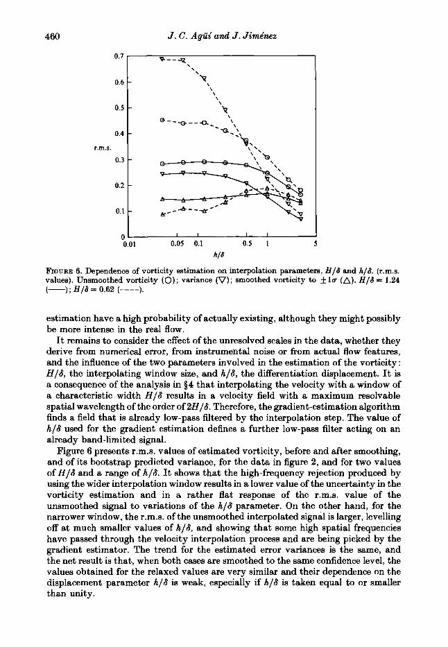
FIQTJRE 6. Dependence of vorticity estimation on interpolation parameters, H / 8 and h/8. (r.m.s. values). Unsmoothed vorticity (0); variance (V); smoothed vorticity to + l r (A). H I S = 1.24 (-) ; H / 6 = 0.62 (----).

estimation have a high probability of actually existing, although they might possibly be more intense in the real flow.

It remains to consider the effect of the unresolved scales in the data, whether they derive from numerical error, from instrumental noise or from actual flow features, and the influence of the two parameters involved in the estimation of the vorticity : H / 6 , the interpolating window size, and h/S, the differentiation displacement. It is a consequence of the analysis in $4 that interpolating the velocity with a window of a characteristic width H / 6 results in a velocity field with a maximum resolvable spatial wavelength of the order of 2H/6 . Therefore, the gradient-estimation algorithm finds a field that is already low-pass filtered by the interpolation step. The value of h/b used for the gradient estimation defines a further low-pass filter acting on an already band-limited signal.

Figure 6 presents r.m.8. values of estimated vorticity, before and after smoothing, and of its bootstrap predicted variance, for the data in figure 2, and for two values of H I 6 and a range of h/6. It shows that the high-frequency rejection produced by using the wider interpolation window results in a lower value of the uncertainty in the vorticity estimation and in a rather flat response of the r.m.8. value of the unsmoothed signal to variations of the h/6 parameter. On the other hand, for the narrower window, the r.m.8. of the unsmoothed interpolated signal is larger, levelling off a t much smaller values of h/S, and showing that some high spatial frequencies have passed through the velocity interpolation process and are being picked by the gradient estimator. The trend for the estimated error variances is the same, and the net result is that, when both cases are smoothed to the same confidence level, the values obtained for the relaxed values are very similar and their dependence on the displacement parameter h/S is weak, especially if h/6 is taken equal to or smaller than unity.

On the performance of particle tracking 46 1

The situation, however, is not completely satisfactory, in that there is no guarantee that the resulting vorticity values are ‘true’, but only that they are ‘conservative’, in the sense that they are no larger than they should be. This is probably the best that can be done. The procedure sketched here retains as much information as possible from the scales of the flow that can actually be observed, and may be in error because of flow features that are below the observation limit. But those features are, by definition, unobservable. The situation was different in the case of the velocity field, in which we had an a posteriori method of checking our results, and could give a true estimate of the error included.

The vorticity maps presented in the next section have been derived using the wider interpolation window of the two used in figure 6, and h/S equal to unity.

7. Experimental results The results of processing the traces in figure 2 are shown in figure 7, which includes

both components of velocity and vorticity. As is usually the case with vortex wakes, the longitudinal velocity is not very informative, but both the transversal velocity and the vorticity show clearly the alternating structure of the vortex street.

The area represented in the figure covers approximately 7 x 11 diameters (cm) on the flow, beginning 11 diameters downstream from the cylinder. All values were interpolated to a 20 x 30 grid and smoothed to within & cr. The grid interval corresponds roughly to half the minimum observable wavelength and, therefore, the smallest details in figure 6 correspond approximately to the highest available resolution.

Figure 8 shows the vorticity maps resulting from three consecutive frames of the wake. The concentrations of alternating vorticity can be seen clearly, as well as their convective movement downstream. The time interval between frames is 0.61 s, and we estimated the convection velocity to be around 12 cm/s, measured with respect to the cylinder, which corresponds to a translation of the eddies by about one half of the frame length for each frame interval. Since the free-stream velocity is 18 cm/s, this convection velocity is somewhat low, but in the range given by other investigators (Cantwell & Coles 1983; Schaefer & Eskinazi 1959). The width of the area shown in the figure corresponds to the full width of the test channel, and the vorticity of the boundary layers is visible in the map, especially on the upper wall.

An interesting feature of this and the previous figure is the relative abundance of vortices containing two vorticity maxima, and the presence of small, randomly distributed, vorticity concentrations. Split vortices have been observed before in the near wake, at similar Reynolds numbers, both in numerical simulations (Davis & Moore 1982), and in visualizations of flows behind accelerating bluff bodies (Freymouth, Bank & Palmer 1985). The process of vortex tearing and reorganization seems to be an integral part of the way in which the wake attains its equilibrium state.

The uncertainties associated with the data in figures 7 and 8, before smoothing are large. The r.m.8. values of the velocity fluctuation in all frames are similar, u’/8 x v’/8 x 0.1, which is consistent with previously published values when they are averaged across the wake. The amount of data in our case was not enough to obtain a reliable turbulent intensity profile. The corresponding r.m.8. values of the expected interpolation errors in velocity are 0.030 for u, and 0.028 for v. These values are Class-3 bootstrap estimates, and they should be added quadratically to

462

u- urn

J . C. Agiii and J . Jiminez

FIQURE 7. (a) Longitudinal velocity, (b ) transversal velocity, and (c) dimensionless vorticity, oD/Urn derived from the data in figure 2. Urn = 18 cm/s. All results are smoothed to plus-minus one standard deviation. Distance between isolines is 0.8 cm/s in velocity and 0.1 in vorticity, and isolines are symmetric about zero. Dashed lines correspond to negative values.

On the performance of particle tracking 463

FIQURE 8. Vorticity map for three consecutive frames of the cylinder wake. Isolines and parameters as in figure 7 (c). Limits of map are 5 and 23 cylinder diameters, left to right. Convection velocity is about 7 diameters/frame, so that the first two vortices of the first frame correspond to the last two of the last one.

the approximately 0.050 error expected from the visualization method. The resulting 0.060 expected total error is a small percentage of the average velocity of the particles, but is equal to 60 % of the velocity fluctuations. However, the maps in the figures have been smoothed to within one standard deviation, and the probability that the features shown actually exist is relatively high (65-70 %).

A final result is presented in figure 9, which shows the peak vorticity values for the eddies that form the wake. This measurement is difficult to do by any other means, and we have only been able to find published results in two other cases, corresponding to wakes at fairly different flow conditions and at non-overlapping downstream ranges. All values are drawn together in our figure. The values from Imaichi & Ohmi (1983) are particle-tracing results, but refer to the extremely near wake at fairly low Reynolds number (cz 200), while those from Cantwell & Coles (1983) are flying-

464 J . C. Agui and J . Jiminez

A O I O

0 5 10 15 20 25

X l D

FIQURE 9. Peak magnitude of vorticity in eddies in the wake aa a function of downstream distance. 0, Imaichi & Ohmi (1983), Re = U , D / v = 200; V, Cantwell & Colea (1983), Re = 14OOOO; Open symbols, present work (k lo), Re = 2000.

hot-wire, phase-averaged, measurements on a wake at high Reynolds numbers ( x 140000). Our flow has a Reynolds number in between the two extremes and extends Cantwell 8z Coles results downstream.

Even so, the results seem to form a coherent picture, in which the eddies appear near the cylinder as compact cores, and relax to a more extended equilibrium configuration about 10 cylinder diameters downstream. Defining the eddy turnover time as A/v', where v' is the r.m.s. transversal velocity fluctuation, and A is a characteristic wake wavelength, this corresponds to just one or two eddy turnovers. This suggests that the relaxation process is inviscid, which agrees with the fact that measurements from flows with widely different Reynolds numbers seem to agree approximately.

8. Simultaneous laser measurements To validate the results of the particle- tracking technique, we have conducted

simultaneous measurements of the velocity at one point in the interior of the wake using both particle tracing and laser-Doppler anemometry.

The laser-Doppler equipment was a 15 mW He-Ne laser and a single-channel TSI Counter Model 1980 connected to a PDP-11/04 computer. The experimental arrangement is shown in figure 10. The decoupling between the camera and the photomultiplier tube of the LDA was achieved by placing appropriate optical filters in front of the two systems. Since the amount of light reaching the camera was cut substantially by the filter, it was assumed that only the largest particles would show in the pictures, and that the effective illumination interval was the one corresponding to the maximum intensity of the pulse, which was monitored with a photodiode.

The hardest problem was the synchronization of the measurements from the camera and from the anemometer. Large particles have a tendency to produce spurious readings in the LDA and their signals were filtered at the counter. As a consequence, the data rate was rather low, and several of the pictures used in partiole tracking had no corresponding LDA data. Every time a picture was taken, a bit was raised in the laser data being acquired at the time and, in addition, each laser data

FIGURE 10.

On the performance of particle tracking

6c Experimental &-up for simultaneous laser-Doppler and particle-tracking

24

22

20

u*** (cm/s)

18

16

measurement.

,

&'"' I

' I

I I'

465

velocity

I I I I

14 16 18 20 22 24 14 I

U,*" (cm/s)

FIGURE 11. Simultaneous laser-Doppler anemometry and particle-tracking velocity measurement. Flow parameters are approximately the same as in the rest of the paper.

point contained its acquisition time to help in synchronizing with the camera. These times, however, contained occasional errors, due to the overflow of a counter in the system, and some of the identifications between pictures and data were ambiguous. Moreover, the experiment itself was messy and we were only able to accumulate eight pairs of data for which both the particle-tracking and laser data were reasonably secure.

Each particle-tracking velocity measurement derived from 4-5 different particles. It was interpolated to the focal volume of the laser using a narrow interpolating

466 J . C. Agui and J . JimLnez

window, and its r.m.s. error was estimated by bootstrapping. Since the area of the flow studied in this case was much smaller than before, it was possible to use larger optical magnifications, and the visualization error was considered negligible. On their part, each record of useful LDA data contained 3 4 measurements. Their average was taken as a representative value, and their standard deviation, as a measure of error.

Figure 11 is a cross-plot of laser against particle-tracking data. The error bars, in both cases, are plus-minus one standard deviation. While eight data sets are too few for any serious statistical analysis, both sets seem to correspond reasonably well within their respective errors.

9. Conclusions We have reviewed several of the sources of error associated with particle-tracing

techniques as applied to the measurement of velocity and vorticity fields in moderate-Reynolds-number turbulent flows in liquids. The analysis is based both on theoretical estimates and on a specific experiment on the wake of a cylinder.

The results show that the errors associated with visualization and tracking of the particles themselves can be kept within reasonable limits if the trace length is kept in the order of a mm, corresponding to integration times of a few ms for reasonable flow velocities in water, but that this error is given as a fraction of the mean flow velocity, and becomes a substantial fraction of the turbulent velocity signal unless the frame of reference chosen for the picture is such that the magnitude of the velocity fluctuations are comparable to the characteristic mean velocity of the particles.

The errors of interpolation, on the other hand, are always a large fraction of the velocity fluctuations, both because of aliasing due to the limited sampling density and because of the lack of ‘ideal ’ interpolating methods for randomly distributed samples. As discussed in $4, the minimum observable wavelength scales with the resolution with which a particle position can be measured. In our experiment, this resolution is about 0.1 mm, and the minimum observable wavelength stands a t about 6 mm, which is comparable to some of the important turbulent scales in the flow. As a consequence, the sampling errors are large, 20-30%. This is likely to be so in most turbulent flows, unless a way can be found to use particle traces that are much shorter with respect to the flow scales. The development of better optics, which are able to provide a more accurate determination of tracer position, should allow the application of the technique to turbulent flows with better accuracy.

In addition, we have shown that bootstrapping is a practical method for the estimation of the interpolation errors associated to a given visualization picture, that it can be used in the absence of a priori information about the flow being measured, and that it provides error information that allows for the production of ‘safe’ maps which contain only those features that are known to exist with a given probability.

We have also presented simultaneous measurements of velocity using particle tracing and laser-Doppler anemometry that validate the previous results.

Finally, we have applied the method to obtain some measurements on the wake. While the purpose of the experiment was the characterization of the method of measurement, rather than of the flow itself, and, as consequence, the quality of the flow apparatus was low, some of those results are still interesting. The presence of bimodal vorticity distributions in the eddies of the near wake throws some light on the mechanisms of formation of the large structures, while the measurements of peak

On the performance of particle tracking 467

vorticity, which are among the first published, are at least indicative of the rate that the eddies reach their equilibrium structure. They are also roughly consistent with the other known measurements of peak vorticities in wakes.

As a final conclusion, we have shown that particle tracing is a practical tool for the measurement of velocities and vorticities in moderately three-dimensional turbulent flows, but that extreme care should be paid to the effects of interpolation and to the aliasing effect derived from the limited sampling density.

One of the authors (J.C.A.) was supported partially during the research that led to this work by a fellowship from the Spanish Ministry of Education within the program of Formation of Research Personnel. Computer time for the numerical simulations and data processing was provided graciously by the IBM Scientific Centre.

REFERENCES

AGTERBERO, F. P. 1974 Geomathematics, pp. 352-356. Elsevier. CANTWELL, B. & COLES, D. 1983 An experimental study of entrainment and transport in the

CLAYTON, B. R. & MASSEY, B. S. 1967 Flow visualisation in water: a review of techniques. J. Sci.

DAVIS, R. W. & MOORE, E. F. 1982 A numerical study of vortex shedding from rectangles.

DIACONIS, P. & EFRON, B. 1983 Computer intensive methods in statistics. Sci. Am. 248 (5),

DIMOTAKIS, P. E., DEBUSSY, F. D. & KOOCHESFAHANI, M. M. 1981 Particle streak velocity field

EFRON, B. 1979a Bootstrap methods: another look at the Jacknife. Annls Statist. 7 , 1-26. EFRON, B. 19793 Computers and the theory of statistics: thinking the unthinkable. SZAM Rev.

21, 460480. EFRON, B. 1982 The Jacknife, the Bootstrap and other resampling schemes. CBM8-NSF Reg.

Conf. Ser. in App. Math. vol. 38, pp. 29-36. SIAM. EFRON, B. 1983 Estimating the error rate of a prediction rule : improvement on cross-validation.

J. Am. Statist. Assoc. 78, 316-331. EMRICH, R. J. 1981 Methods of Experimental Physics, vol. 18: Fluid Dynamics. Academic

Press. FREYMUTH, P., BANK, W. & PALMER, M. 1985 Further experimental evidence for vortex splitting.

J . Fluid Mech. 152, 28S299. CARABEDIAN, P. R. 1964 Partial differential equutim, pp. 485-492. Wiley. GERRARD, J. H. 1966 The three-dimensional structure of the wake of a circular cylinder. J. Fluid

HJELMFELT, A. T. t MOCKROS, L. F. 1966 Motion of discrete particles in a turbulent fluid. Appl.

HINZE, J. 0. 1959 Turbulence. McGraw-Hill. IMAICHI, K. & OHMI, K. 1983 Numerical processing of flow-visualisation pictures : measurement

JIAN, L. & SCHMITT, F. 1982 Water current determination by picture processing. In Proc. ICASSP

JIMENEZ, J. 1985 Some computational problems in computer-assisted flow visualisation. In Proc.

JIMENEZ, J. & AaUi, J. C. 1987 Approximate reconstruction of randomly sampled signals. Signal

LANDAU, L. D. & LIFSHITZ, E. M. 1959 Fluid Mechania, p. 122. Pergamon.

turbulent near wake of a circular cylinder. J. Fluid Mech. 136, 321-374.

Instrum. 44, 2-11.

J . Fluid Mech. 116, 475-506.

116-132.

measurements in a two dimensional mixing layer. Phys. Fluids 2, 995-999.

Mech. 25, 143-164.

Sci. Res. 16, 149-161.

of two-dimensional vortex flow. J. Fluid Mech. 129, 283-311.

82. Paris, pp. 830-833. IEEE.

Zntl Symp. Compu. Fluid Dyn. Tokyo, pp. 145-156. Japan SOC. Comput. Fluid Dyn.

Proc. 12, 153-168.

468

MATHERON, G. 1972 In Traite de Znformutique Geologique (ed. P. Laffite), pp- 362-378. Masson. MERZKIRCH, W. 1974 Flow Visualization. Academic. PAPAILIOU, D.D. & LYROUDIS, P. S. 1974 Turbulent vortex streets and the entrainment

mechanism of the turbulent wake. J. Fluid Mech. 62, 11-31. PRANDT, L. & TIETJENS, 0. 1934 Applied Hydro and Aerodynamics. Dover. SCHAEFER, J. W. & ESKINAZI, S. 1959 Analysis of the vortex street generated in a viscous fluid.

J . Fluid Mech. 6, 241-260. SOMMERSCALES, E. F. C. 1980 Fluid velocity measurement by particle tracking. In Flow, its

Measurement and Control in Science and Indmtry, vol. I (ed. R. E. Wendt), pp. 795-808. Instrum. SOC. Am.

UTAMI, T. & UENO, T. 1984 Visualisation and picture processing of turbulent flow. Exp. Fluids 2 , 25-32.

UTAMI, T. & UENO, T. 1987 Experimental study of the coherent structure of turbulent open channel flow using visualization and picture processing. J. Fluid Mech. 174, 39M40.

WERLE, H. 1973 Hydrodynamic flow visualisation. Ann. Rev. Fluid Mech. 5 , 361-382.

J . C. Agui and J . Jirninez