GALILEO TRACKING PERFORMANCE UNDER IONOSPHERE SCINTILLATION Nazelie Kassabian

(1), Yu Morton

(2)

(1) Department of Electronics and Telecommunications, Politecnico di Torino, Corso Duca degli Abruzzi 24

10129 Torino, Italy, Email: nazelie.kassabian@polito.it (2)

Department of Electrical and Computer Engineering, Miami University, Oxford, OH 45056 USA, Email:

mortonyt@miamiOH.edu

ABSTRACT

The objective of this paper is to investigate the

ionosphere scintillation impact on the Galileo E1 and E5

open service (OS) BOC signals through the comparison

of carrier to noise ratio, amplitude and phase

scintillation indices. These indices are obtained by

processing correlator and phase measurement outputs of

a customized Galileo software receiver in Matlab on one

side, and a Septentrio PolaRxS PRO receiver on the

other. The collection of global navigation satellite

systems (GNSS) data is performed in an equatorial

region in Ascension Islands where scintillation is known

to be a common event. Code acquisition and tracking

routines are specially tailored to take into account each

frequency band’s signal structure, including chip rate,

primary/secondary code, and dedicated subcarrier.

Considering the pilot channel where no data message is

encoded, the phase lock loop (PLL) uses a coherent

extended arctangent discriminator to accept a wider

carrier phase error. The choice of all these three

strategies is motivated by the desire to maintain receiver

carrier and code phase lock in challenging scintillation

conditions. On the Galileo E1 OS frequency band, the

locally generated code used as a reference to perform

tracking, is comprised of the spreading code multiplied

by a special subcarrier, the composite binary offset

carrier CBOC(6,1,1/11). Due to the shape of the

autocorrelation function of binary offset carrier (BOC)

signals in general, ambiguous tracking is a common

threat. For that reason, an unambiguous code phase

detector is inserted in the delay locked loop (DLL) and a

modified version of the two-step CBOC tracking [1] is

implemented. E5a and E5b signals are treated like

binary phase shift keying (BPSK) signals when separate

frequency bands are considered, and so typical BPSK

DLL tracking is applied. To harness the superior

tracking capability offered by BOC subcarriers, a

wideband front-end is needed inside a Galileo receiver

to capture the entire tracking capability of Galileo

signals. It is expected that Galileo wideband signals

exhibit superior tracking permeability during

scintillation events.

1. INTRODUCTION

As more and more awareness is gained in space weather

and ionosphere disturbances impact on our Earth’s

technical infrastructure, more interest is shed on

studying the underlying physical phenomena related to

the Sun’s activity and consequently ionosphere

scintillation. In that respect, there are many goals to be

achieved on the ground, mainly to curb the potentially

damaging effects of technical equipment such as electric

grids or even avoid outages of global navigation satellite

systems (GNSS) which the economy and world order is

increasingly dependent upon. Moreover, as more and

more GNSS are emerging, such as Galileo, GLONASS

and Beidou, the possibility of exploiting the availability

of a big number of satellites for the end of a global

ionosphere scintillation monitoring system is becoming

more realistic and very much appealing. Radio

frequency (RF) signals undergo amplitude/phase/

frequency scintillation as they pass through the

ionosphere region as a result of solar winds erupted

from the Sun characterized by turbulent ionized gases

called plasma [2]. These ionized gases are dispersive,

meaning that they have a different impact on different

frequencies. Radio signals at the lower frequencies

suffer more from the plasma irregularities. GNSS

receivers is offering an effective tool to monitor the

state of these irregularities in the sky as by recovering

signals transmitted on different frequency bands from

one or more of its spacecrafts. This can be achieved by

monitoring the power of the recovered signal after

performing carrier/code tracking and examining the

resulting detrended carrier phase fluctuations. The

objective of this paper is to develop tracking algorithms

applicable to Galileo signals experiencing ionospheric

scintillation and to evaluate the algorithms performance

using both simulation and real scintillation data.

The remaining paper is organized as the following.

Section 2 describes the current Galileo OS signal

structure. Section 3 presents simulated Galileo signal

generation process. Galileo code and carrier tracking

algorithms are discussed in Section 4. Section 5 applies

the tracking algorithms to real Galileo scintillation data

collected at Ascension Island and compares the

algorithm performance with a commercial receiver

outputs. Section 6 summarizes the work.

2. GALILEO OS SIGNAL STRUCTURE

The Galileo OS signals are open source free of charge

signals to provide competitive position and timing

performance for the user community. The Galileo OS

mainly consists of three frequency bands, E1, E5a/b,

and E6, although the latter will be omitted in this paper

because it is not fully specified in the Galileo OS

interface control document (ICD) [3]. The transmitted

power on both of these frequency bands is divided onto

two channels, the data and pilot channels. Due to plans

to extend the integration time to more than one code

period, only one of these channels is considered in this

paper, the pilot channel.

2.1. Galileo E1 OS Signal

The Galileo E1 frequency band is found in the upper L-

Band and is centered around 1575.42 MHz, the same

center frequency as that of the GPS L1 frequency band.

It is modulated by a ranging code as well as a weighted

sum of two subcarrier signals (higher weight to the

lower rate subcarrier) which together make up the

composite binary offset carrier (CBOC) modulation

CBOC(6,1,1/11) in the time domain. In the frequency

domain, it is known as the modified binary offset carrier

MBOC(6,1,1/11) and its power spectral density (PSD)

is expressed as:

)(611

1)(

111

10)( fGfGf

sG (1)

where G1(f) and G6(f) are the PSD of the binary offset

carrier BOC(1,1) and BOC(6,1) signals. This is the total

PSD of the Galileo E1 in-phase channel. In fact, the E1

signal allocates data/pilot channels on the same in-phase

I channel while the quadra-phase Q channel is reserved

for the public regulated service (PRS) which has a wider

frequency bandwidth. The Galileo OS E1 reference

bandwidth is specified to be β = 24.552 MHz as

compared to the GPS L1 and the E5a/b reference

bandwidths of 20.46 MHz. In fact, a theoretical two-

sided bandwidth that accommodates both BOC(1,1) and

BOC(6,1) signals can be assessed to be equal to

2*(6*1.023 + 1.023) = 14.322 MHz. It can be concluded

that such a bandwidth covers a large percentage of the

total signal power spectrum after looking at the power

loss or even correlation loss [4] defined as:

(2)

In fact, the choice of a 14.322 MHz as a baseband

receiver bandwidth induces a correlation loss of 0.5 dB

as seen in Fig. 1 and can be considered negligible. The

pilot channel subcarrier is equal to the weighted

difference between the narrowband and the wideband

signals BOC(1,1) and BOC(6,1) respectively. The data

channel subcarrier is equal to the sum of the

aforementioned signals and is orthogonal to the pilot

channel subcarrier. As a consequence, a certain

orthogonality exists to separate the data from the pilot

channels.

The Galileo E1 OS signal ranging codes are composed

of primary and secondary codes by using a tiered code

Figure 1. Correlation loss in dB due to bandlimiting

construction [3]. The primary code chip rate is 1.023

Mcps, similar to the GPS L1 C/A and GPS L1C signals.

The primary code length is 4 ms and its length is 4092

chips. The primary codes of the data/pilot channels are

long pseudorandom noise (PRN) optimized memory

codes and are published in the Galileo OS ICD [3]. The

secondary code on the pilot channel is unique for all

satellites. The data channel is deprived of a secondary

code but instead is multiplied by the navigation data,

while the pilot channel is deprived of the navigation

data and multiplied by a secondary code of length 25

chips and duration 100 ms. Fig. 2 shows the Galileo E1

OS normalized autocorrelation function for both data

and pilot channels and how they relate to the

corresponding BOC(1,1) signal. It is assumed a

sampling frequency of 16.367 MHz.

Figure 2. Galileo E1 OS auto-correlation functions

2.2. Galileo E5 OS Signal

The Galileo E5a frequency band is found in the lower

L-Band and is centered around 1176.45 MHz, the same

center frequency as that of the GPS L5 frequency band.

The Galileo E5b frequency band is centered around

1207.14 MHz and both these bands have a bandwidth of

20.46 MHz [3]. If the entire E5 wideband signal is

considered as in an AltBOC modulation, then the

existence of subcarriers is imperative. However, the

E5a/b signals, when considered as separate frequency

bands, are QPSK signals, or even BPSK signals with a

chipping rate of 10.23 MHz when one of the data/pilot

orthogonal channels is taken into account. Therefore,

the minimum sampling frequency that satisfies the

2/

2/

)(

fGS

Nyquist sampling theorem at baseband is 20.46 MHz.

Moreover, unlike the Galileo E1 OS channels, the E5a/b

data/pilot channels are characterized by orthogonality.

Both of these channels primary PRN codes can be

generated using linear feedback shift registers and last

1ms while the secondary codes are published in

hexadecimal format in [3]. The data channel offers a

unique secondary code for all satellites (20 ms for E5a

data channel and 4 ms for E5b data channel) while a

different secondary code of 100 ms is used for every

satellite on the pilot channel. The auto-correlation

function of the E5a/b Galileo signals shown in Fig. 3 is

the typical BPSK auto-correlation function (similar to

that of GPS L1 C/A code) where a single peak is present

at zero phase lag.

Figure 3. Galileo E5a OS auto-correlation functions

3. SIGNAL/IONOSPHERE SCINTILLATION

SIMULATION AND ESTIMATION

The received or reference signal s[m] at the input of a

GNSS receiver can be generically expressed as:

][])[2cos(][][2][ mnmS

mTc

fmcmdPms (3)

where P is the total received signal power, d[m] is a

binary data sequence holding the navigation message,

c[m] is the spreading code (which includes the

subcarrier code sc[m] in BOC modulated signals), fc is

the carrier frequency, TS is the analog to digital

sampling interval, φ[m] is the instantaneous carrier

phase and n[m] is a noise term which represents thermal

noise and is assumed to be white with a single sided

PSD of N0 Watts/Hz.

3.1. Galileo Signal Simulation

Galileo E1 and E5a/b OS signal (data and pilot

channels) simulation routine is developed to be used in

this paper, where a set of parameters can be specified to

generate the desired simulated signals. These

parameters include the frequency band to be generated,

the intermediate frequency fIF, the sampling frequency

fS, the Doppler frequency fD, the Doppler rate aD, the

PRN or space vehicle (SV) number, the spreading code

phase or code delay τ, the carrier to noise ratio (CNR)

C/N0, the time duration over which the signal is to be

simulated TD. There is also the option to exclude any of

the code, carrier and noise signals giving the

opportunity to test and analyze the mechanisms at the

heart of carrier phase and code delay tracking. Given the

aforementioned two-sided reference bandwidth values

of 24.552 and 20.46 MHz of the Galileo E1 and E5a/b

OS signals, the intermediate frequency should be

carefully chosen so as to be greater than the single sided

reference bandwidth values 12.276 MHz and 10.23

MHz respectively so as to avoid aliasing with the

negative side of the spectrum. The sampling frequency

should then be chosen so as to satisfy the Nyquist

sampling theorem (twice the bandwidth). The

methodology followed in generating the simulated

signals is a structured approach where modular

functions perform unique duties: the baseband code is

produced in terms of chips over the period of a

secondary code which is 100 ms for both E1 and E5a/b

pilot channels; the data channel is generated by

repeating the primary code until the same length is

reached. Basically, this step involves the multiplication

of the primary and secondary codes following a tiered

code structure. A non-return-to-zero (NRZ) signal is

generated by mapping the logical binary values 0 and 1

to +1 and -1 respectively. The next step for the E1 OS

signal is to multiply each chip by the 12 sub-chips of the

corresponding CBOC. The E5a/b signals skip this step

because there is no subcarrier. After that step, it is

necessary to shift the code by the complement of the

desired code phase, and then to sample with the desired

fS taking into account the desired Doppler frequency

and rate. The reason for introducing the code phase shift

in terms of chips rather than samples and hence the

process of shifting before sampling, is because with a

nonzero Doppler frequency, the effective code phase in

samples changes at every block of signal simulation, i.e.

100 ms in our case. Finally the data message is

generated using the random function and with the

specified data rate in the ICD [3]. The last stage is to

simulate the front end and the Doppler frequency on the

carrier, and this is done by multiplying the baseband

signal by the cosine and sine of the appropriate

frequency (the I and Q channels) as in Eq. 3, that is

setting the frequency as:

(4)

In this paper, real GNSS baseband signals are available

at the input of the GNSS receiver at hand, therefore the

intermediate frequency is set to 0 Hz in the rest of the

paper, and the sampling frequency is chosen to be 25

Msamples/s. A sample noiseless Galileo E1 OS signal is

Figure 4. Noiseless Galileo E1 and E5a OS PSD

SmT

Da

Df

IFf

cf

generated setting the input parameters to some arbitrary

values, i.e. fD = 2 KHz, aD = -0.2 Hz/s, a code delay of

20560 chips (5 secondary chips and 100 primary chips),

and a time duration TD = 2 seconds. Since there is no

noise in this signal, it is possible to verify the shape of

the MBOC(6,1,1/11) signal spectrum as shown in Fig.

4. A similar signal is generated to verify the E5a PSD as

shown in Fig. 5.

3.2. Ionosphere Scintillation Simulation

The ionosphere scintillation is simulated in addition to

the Galileo OS signal, taking into account the impact

over the amplitude and phase of the original Galileo

signal. The ionosphere scintillation model described in

[5] is used to simulate ionosphere scintillation where

two inputs, the standard scintillation amplitude index S4

and the channel decorrelation time τ0, determine the

amplitude and phase disturbance over the ultra high

frequency (UHF) L-band signals. These two parameter

inputs indicate the severity and speed of the scintillation

in terms of amplitude and phase fluctuations. A possible

improvement to this model would be to control the

speed of the fluctuations in the amplitude and phase

time history separately. The model in [5] is used in this

paper and is deemed realistic as it draws on an extensive

set of equatorial scintillation data to approximate the

signal propagation channel, namely by estimating both

the scintillation amplitude distribution as well as the

spectrum of the complex scintillation signal. A

relatively medium scintillation characterized by a large

S4 index value and a low τ0 value is simulated and

shown in Fig. 6 where S4 and τ0 are set to 0.6 and 0.8

seconds respectively.

Figure 5. Simulated scintillation signal amplitude and

phase to be multiplied and added respectively to the raw

Galileo simulated signal.

3.3. Ionosphere Scintillation Indices

During GNSS signal tracking, I and Q prompt correlator

outputs are logged as indicators of how much power is

recovered from the received signal. In fact, the CNR

and the S4 index computations are based on the signal

intensity SI which is equal to the difference of

narrowband and wideband power [6]:

2

22

4

IS

IS

IS

S (5)

where <.> is the expected value. In fact, S4 is a

normalized standard deviation of signal intensity and is

normally computed on 60 second intervals. Narrowband

and wideband power values are computed every 20 ms

using multiple I and Q correlator values, i.e. M=5 for

Galileo E1 OS and 20 for Galileo E5a/b:

2

1

2

1

M

ii

QM

ii

INBP (6)

M

ii

Qi

IWBP

1

22 (7)

This is due to the different accumulation intervals used

on the two frequency bands respectively which is

determined by their code periods, i.e. 4 ms for Galileo

E1 OS and 1 ms for Galileo E5a/b. However, this does

not prevent a fair comparison between the two signals

as it has been proved in [7] that using the normalization

in the S4 computation, removes any dependence of S4

on the accumulation interval TI. Finally, the need for

detrending arises due to the dependence of the signal

intensity measurements on the satellite receiver

dynamics (D), the receiver oscillator phase error (O),

the ionosphere (I) and troposphere (T) errors,

collectively known as DOIT terms. For that end, a 6th

order Butterworth low pass filter is used with a cutoff

frequency of 0.05 Hz instead of the traditional 0.1 Hz

[7]. The detrended signal intensity is obtained by

dividing the raw signal intensity by the low pass filter

output adjusted by the filter group delay:

LPFWBPNBP

WBPNBP

IS

)(

(8)

Moreover, the S4 due to ambient noise has to be

removed from the squared value of the S4 index:

oNC

oNC

oN

S/19

5001

/

100

4

(9)

where C/N0 can be estimated using the I and Q

correlator outputs following the power ratio method [8].

On the other hand, the traditional phase scintillation

index σφ is the standard deviation of the accumulated

Doppler range (ADR) which is the accumulation of the

estimated phase by the phase locked loop (PLL) during

the integration interval and the carrier discriminator

phase error σE:

])[][ˆ2( kTkfstdk

EID

(10)

However, before computing the standard deviation, the

carrier phase measurements as the signal intensity

measurements, should be detrended as well to ward off

DOIT trends. The detrending is applied at post-

processing through a 6th

order Butterworth high pass

filter with a cutoff frequency of 0.05 Hz [7].

Consequently, the standard deviation of the detrended

carrier phase measurements is computed every 30

seconds.

4. CARRIER/CODE TRACKING

IMPLEMENTATION AND VALIDATION

A digital PLL (DPLL) is a proportional integral (PI)

control loop which basically tracks the carrier phase of

the input signal such that it maintains a zero steady state

phase error. A digital delay locked loop (DDLL) is the

spreading code phase counterpart. GNSS carrier

tracking loops typically use a second/third order DPLL

while the code tracking loop can be either a first order

carrier aided loop or a second order unaided loop.

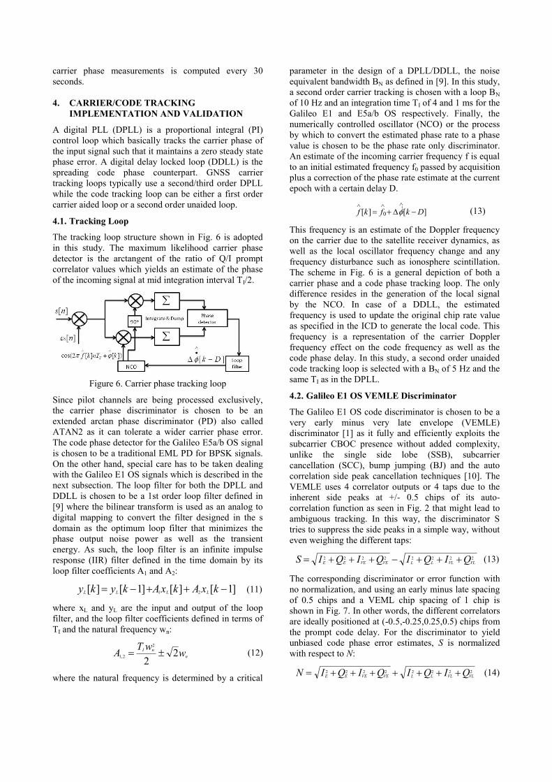
4.1. Tracking Loop

The tracking loop structure shown in Fig. 6 is adopted

in this study. The maximum likelihood carrier phase

detector is the arctangent of the ratio of Q/I prompt

correlator values which yields an estimate of the phase

of the incoming signal at mid integration interval TI/2.

Figure 6. Carrier phase tracking loop

Since pilot channels are being processed exclusively,

the carrier phase discriminator is chosen to be an

extended arctan phase discriminator (PD) also called

ATAN2 as it can tolerate a wider carrier phase error.

The code phase detector for the Galileo E5a/b OS signal

is chosen to be a traditional EML PD for BPSK signals.

On the other hand, special care has to be taken dealing

with the Galileo E1 OS signals which is described in the

next subsection. The loop filter for both the DPLL and

DDLL is chosen to be a 1st order loop filter defined in

[9] where the bilinear transform is used as an analog to

digital mapping to convert the filter designed in the s

domain as the optimum loop filter that minimizes the

phase output noise power as well as the transient

energy. As such, the loop filter is an infinite impulse

response (IIR) filter defined in the time domain by its

loop filter coefficients A1 and A2:

]1[][]1[][ 21 kxAkxAkyky LLLL (11)

where xL and yL are the input and output of the loop

filter, and the loop filter coefficients defined in terms of

TI and the natural frequency wn:

n

nIw

wTA 2

2

2

2,1 (12)

where the natural frequency is determined by a critical

parameter in the design of a DPLL/DDLL, the noise

equivalent bandwidth BN as defined in [9]. In this study,

a second order carrier tracking is chosen with a loop BN

of 10 Hz and an integration time TI of 4 and 1 ms for the

Galileo E1 and E5a/b OS respectively. Finally, the

numerically controlled oscillator (NCO) or the process

by which to convert the estimated phase rate to a phase

value is chosen to be the phase rate only discriminator.

An estimate of the incoming carrier frequency f is equal

to an initial estimated frequency f0 passed by acquisition

plus a correction of the phase rate estimate at the current

epoch with a certain delay D.

][][ 0 Dkfkf

(13)

This frequency is an estimate of the Doppler frequency

on the carrier due to the satellite receiver dynamics, as

well as the local oscillator frequency change and any

frequency disturbance such as ionosphere scintillation.

The scheme in Fig. 6 is a general depiction of both a

carrier phase and a code phase tracking loop. The only

difference resides in the generation of the local signal

by the NCO. In case of a DDLL, the estimated

frequency is used to update the original chip rate value

as specified in the ICD to generate the local code. This

frequency is a representation of the carrier Doppler

frequency effect on the code frequency as well as the

code phase delay. In this study, a second order unaided

code tracking loop is selected with a BN of 5 Hz and the

same TI as in the DPLL.

4.2. Galileo E1 OS VEMLE Discriminator

The Galileo E1 OS code discriminator is chosen to be a

very early minus very late envelope (VEMLE)

discriminator [1] as it fully and efficiently exploits the

subcarrier CBOC presence without added complexity,

unlike the single side lobe (SSB), subcarrier

cancellation (SCC), bump jumping (BJ) and the auto

correlation side peak cancellation techniques [10]. The

VEMLE uses 4 correlator outputs or 4 taps due to the

inherent side peaks at +/- 0.5 chips of its auto-

correlation function as seen in Fig. 2 that might lead to

ambiguous tracking. In this way, the discriminator S

tries to suppress the side peaks in a simple way, without

even weighing the different taps:

22222222VLVLLLVEVEEE QIQIQIQIS (13)

The corresponding discriminator or error function with

no normalization, and using an early minus late spacing

of 0.5 chips and a VEML chip spacing of 1 chip is

shown in Fig. 7. In other words, the different correlators

are ideally positioned at (-0.5,-0.25,0.25,0.5) chips from

the prompt code delay. For the discriminator to yield

unbiased code phase error estimates, S is normalized

with respect to N:

22222222VLVLLLVEVEEE QIQIQIQIN (14)

In addition, a normalization factor is needed such that

the piece-wise linear discriminator function has a unity

slope for a specific piece in consideration. In fact, the

idea of coarse and fine tracking as mentioned in [1]

stems from the fact that the discriminator function can

be approximated by a collection of several piece-wise

linear functions which have different slopes. This is due

to the CBOC(6,1,1/11) auto-correlation shape as shown

in Fig. 2. Due to this CBOC shape, namely the quasi

zero slope of the auto-correlation function main peak

around +/- 0.1 chips, there is an inherent risk of

confining to sub-optimal code tracking, incurring a

position error of the order of 150 meters. For this

reason, coarse and fine tracking need to be carried out

successively. Coarse tracking is initiated and a test is

performed to assess the feasibility of moving to fine

tracking. In other words, this means monitoring the

range of estimated code delay error values at the

VEMLE discriminator output and raising a flag when

these errors are small enough in a statistical sense. A

simple arbitrary monitoring test consists of looking back

over the last second of tracking, and moving to fine

tracking if 90% of the code delay values are less than

half of the fine tracking linear region, which is half of

an early minus late chipping space value, i.e. 0.25/2 =

0.125 chips. On the other hand, another condition has to

be satisfied to remain in the fine tracking stage once

there, that is 50% of the code delay error values in the

last 100 ms are required to be less than 0.125 chips. In

the design of the coarse/fine tracking, the normalization

factors are selected according to the slope of the code

auto-correlation function main peak as well as the early

minus late chip spacing. Analytical expressions of these

normalization factors can be found in [1] where an

additional multiplicative factor of 2 is used for coarse

tracking, and 1/1.2 for fine tracking. Figure 7 shows all

three versions, without normalization, with

normalization for coarse and fine tracking. It can be

seen that coarse tracking ensures a wide linear range

between +/- 0.5 chips and partially between +/- 1 chip.

In the same figure, it can be seen that fine tracking, on

the other hand, ensures a narrow linear range but

specifically concentrated around zero code delay error.

This yields fine or accurate estimates of the code phase

error.

Figure 7. VEMLE discriminator with different

normalization options

4.3. Tracking of Simulated Signals

A sample Galileo E1 signal is simulated setting the

input parameters to some arbitrary values, i.e. fD = 2

KHz, aD = -0.2 Hz/s, a code delay of 20560 chips (5

secondary chips and 100 primary chips), a CNR of 45

dB-Hz over a time duration TD = 2 seconds. Applying

the tracking scheme described in the previous section

yields the results shown in Fig. 8, where the true and

estimated carrier frequency are shown during each

integration interval as well as the total phase error

where the steady state 95 percentile yields +/- 1.25

degrees. In addition, the DDLL converse is shown

where the estimated code frequency error 95 percentile

lies between +/- 1 degree. On the other hand, the code

phase steady state error 95 percentile lies between +/-

0.1 samples. It is worth noting that the higher jitter in

code phase/frequency estimation error at the beginning

is due to the early coarse tracking algorithm and the

transition to fine tracking results in a much lower

tracking jitter. A similar tracking test with E5a/b signals

is performed where carrier/code frequency and phase

errors are shown in Fig. 9.

Figure 8. Tracking output of simulated E1 signal

Figure 9. Tracking output of simulated E5a signal

4.4. Tracking of Simulated Ionosphere Scintillation

In order to assess ionosphere scintillation tracking,

similar Galileo E1 and E5a OS signals are generated

where the scintillation amplitude and phase time history

is incorporated in the original signal as described in

Section 3.2. The S4 index is chosen to be 0.8 and the

channel decorrelation time τ0 to be 0.8. Moreover, the

scintillation indices are derived using the tracking

outputs, mainly the correlation values and the ADR as

described in Section 3.3. Fig. 10 shows that a good

estimate of the S4 index is reached at every minute for

both frequency bands, in the range of 0.55-0.7

compared to an accurate estimate of 0.8 which is not

possible because of the statistical nature of the input

signal due to both noise and scintillation history, and

due to the impact of the tracking loop itself [11]. The S4

estimate discrepancy between the E1 and E5a frequency

bands ranges between 0.02 and 0.1. On the other hand, a

τ0 value of 0.8 results in a σφ estimate in the range of 0.4

to 1 radians. The theoretical σφ range between 0.4 and

0.7 radians is computed using the standard deviation of

the scintillation phase time history for every 30 seconds

and a good estimate is evaluated on both frequency

bands (almost the same) with an error in the range of 0-

0.5 rad. The first two minutes σφ outputs are discarded

due to the ADR detrending filter transient.

Figure 10. Estimated scintillation indices of a simulated

scintillation signal with an S4 intensity of 0.8 and a τ0

value of 0.8 on top of raw Galileo E1 and E5a signals

5. TRACKING OF REAL IONOSPHERE

SCINTILLATION IN GALILEO SIGNALS

Experimental GNSS data has been collected on the 7th

to 10th

of March 2013 at Ascension Island which is

located in the Equator at a longitude of 14.4o W and

latitude of 7.9o S. The data collection has been

performed using flexible and reconfigurable universal

software radio peripheral (USRP) devices, the USRP

N210 acting as an RF front-end. A common antenna,

the Novatel GPS-703-GGG wideband antenna is shared

among five different USRPs acting on different

frequency bands to collect GPS, Galileo E1 and E5,

GLONASS, and Beidou data. In fact, an 8 way splitter

delivers the same data to five USRP N210 and a

Septentrio PolaRxS which houses an oven controlled

crystal oscillator (OCXO) characterized by low noise on

the phase measurements. The OCXO timing signal is

distributed to the various USRPs through an 8 way

passive splitter. The USRP N210 sampling frequency is

set to 25 Msamples/s and delivers a complex signal such

that the effective sampling frequency is 50 Msamples/s.

The Septentrio tracking outputs (I/Q correlator values

and ADR) are saved and used to generate the S4 and σφ

indices as well as the CNR values for a later comparison

with those obtained using the tracking outputs of a

customized receiver as described in this paper.

It is shown in Fig. 11-12-13 that the comparison

between these outputs is fairly satisfying considering

the same SV with PRN 19 and processing different

frequency bands Galileo E1 and E5a. Fig. 11 shows that

the amplitude scintillation is stronger on the E5a band;

similarly Fig. 12 shows that the phase scintillation is

stronger on the E5a band, and Fig. 13 underlines the

possibility of losing lock after going to very low CNR

values.

Figure 11. Filtered S4 estimates on PRN 19 using

Galileo E1 (left) and E5a (right) frequency bands.

Figure 12. Filtered σφ estimates on PRN 19 using

Galileo E1 (left) and E5a (right) frequency bands.

Figure 13. Carrier to noise ratio estimate on PRN 19

using Galileo E1 (left) and E5a (right) frequency bands.

Similar plots can be obtained for SV with PRN 20,

where the scintillation is found to be of significantly

lower intensity. In fact, this can be seen in Fig. 14 where

a proportional relationship is found between the

scintillation indices S4 and σφ on two frequency bands,

the E1 and E5a bands and for different visible satellites.

It is worth mentioning that during the data collection,

SV 19 was following a path going from west to east

with an elevation in the range of 30-40 degrees.

Similarly SV 20 was following a path going from west

to east, passing almost through the same point in space

as SV 19 with a delay of 2.5 hours, but from then on

with a steadily decreasing elevation angle from 50 to 15

degrees. These are the key situations where the

scintillation phenomenon can be studied with a time

resolution determined by the GNSS satellites path.

Unfortunately, the Galileo SV with PRN 11 became

visible during only a short period of time, with an

elevation angle less than 15 degrees, and so had to be

neglected. Finally Galileo SV with PRN 12 had an

interesting path starting from an invisible state to an

increasing elevation from the horizon to a maximum of

40 degrees always in the west part of the sky and even

passing almost through the same point in space as SV

19 with a delay of 2 hours. It can be thus concluded that

in the same region of space the scintillation intensity

becomes considerably higher further later in time, after

comparing the performance of PRN 19 vs PRN 12 as

can be seen in Fig. 14.

Figure 14. Comparison of estimated scintillation indices

on two Galileo frequency bands and three Galileo

satellites.

6. CONCLUSION

Space weather effects, mainly amplitude and phase

scintillation on recently collected UHF Galileo OS

signals have been shown in this paper as these signals

passed through the ionosphere and reached Ascension

Island, an equatorial region. It has been seen that the

recently launched four Galileo satellites add further

observability to the existent block of GNSS satellites in

view of a better time resolution in ionosphere

scintillation monitoring. Exploiting the full wide-

bandwidth offered by the E1 and E5a Galileo signals,

carrier/code tracking has been tested on simulated

signals with and without amplitude/phase scintillation

and performed on real Galileo signals as well. A new

method for Galileo CBOC code tracking has been

proposed. Scintillation indices on three Galileo visible

satellites during data collection have been computed and

compared to the indices generated by the tracking

outputs of a professional Septentrio PolaRxS PRO

scintillation receiver. Finally, the empirical relationships

of the scintillation indices between different frequency

bands have been verified with real Galileo signals on

the E1 and E5a bands.

ACKNOWLEDGMENT

The authors wish to acknowledge funding support from

MIUR the Italian Ministry of Education, University and

Research and US Air Force Research Laboratory

(#FA8650-08-D-1451). The authors also want to thank

Dr. Todd Pedersen and his colleagues from AFRL

Kirkland AFB who supported the Ascension Island data

collection experiment, and Steve Taylor, a graduate

student at Miami University for helping with data

extraction for this project.

REFERENCES

1. A. Jovanovic, C. Mongrédien, Y. Tawk, C. Botteron,

and P. A. Farine (2012). Two-Step Galileo E1

CBOC Tracking Algorithm: When Reliability and

Robustness Are Keys! International Journal of

Navigation and Observation, vol. 2012, Article ID

135401, 14 pages. doi:10.1155/2012/135401

2. C. M. Ho, M. K. Sue, A. Bedrossian, and R. W.

Sniffin (2002). Scintillation Effects on Radio

Wave Propagation Through Solar Corona. Proc.

27th URSZ General Meeting, Maastricht,

Netherlands.

3. European GNSS (Galileo) Open Service Signal In

Space Interface Control Document (SIS ICD)

(2010), Technical report, Brussels.

4. J. W. Betz (2000). Design and Performance of Code

Tracking for the GPS M Code Signal. Proc. 13th

International Technical Meeting of the Satellite

Division of The Institute of Navigation (ION GPS

2000), pages 2140-2150, Salt Palace Convention

Center, Salt Lake City, UT.

5. Humphreys, T.E., M.L. Psiaki, J.C. Hinks, B.W.

O’Hanlon and P.M. Kintner, Jr. (2009). Simulating

Ionosphere-Induced Scintillation for Testing GPS

Receiver Phase Tracking Loops. IEEE Journal of

Selected Topics in Signal Processing, Vol. 3, No.

4.

6. Van Dierendonck, A. J., Klobuchar, J., and Hua, Q.

(1993). Ionospheric Scintillation Monitoring Using

Commercial Single Frequency C/A Code

Receivers. Proceedings of ION GPS-93, Salt Lake

City, UT, pp. 1333 – 1342.

7. Niu, F. (2012). Performance of GPS Signal

Observables Detrending Methods for Ionosphere

Scintillation Studies. (Electronic Thesis or

Dissertation). Miami University. Retrieved from

https://etd.ohiolink.edu/

8. Van Dierendonck, A. J. (1996) GPS Receivers In B.

W. Parkinson, J. J. Spilker, P. Axelrad, and P.Enge

(Eds.), Global Positioning System: Theory and

Applications, vol. 1, American Institute for

Aeronautics and Astronautics.

9. Kaplan E. D. (1996) Understanding GPS: Principles

and Applications. Artech House, Boston, London.

10. Scott Gleason and Demoz Gebre-Egziabher (2009).

GNSS applications and methods, Artech House,

Boston, Massachussets.

11. Mao, X., Y. Morton (2013), GNSS Receiver Carrier

Tracking Loop Impact on Ionosphere Scintillation

Signal C/N0 and Carrier Phase Estimation, Proc.

ION GNSS+, Nashville, TN.