
Enhanced Receiver Techniques for Galileo E5 AltBOC Signal ...
308
-
Upload
khangminh22 -
Category
Documents
-
view
5 -
download
0
Transcript of Enhanced Receiver Techniques for Galileo E5 AltBOC Signal ...

Enhanced Receiver Techniques for Galileo E5AltBOC Signal Processing
By
Nagaraj Channarayapatna Shivaramaiah
A thesis submitted for the degree of
Doctor of Philosophy
Surveying & Spatial Information Systems,
The University of New South Wales.
June 2011

Abstract
In Global Navigation Satellite Systems (GNSS) the structure of the signal predom-
inately determines the system performance and wideband signals, in general, o�er good
performance. Consequently signal design and the receiver processing for wideband signals
have attracted signi�cant research attention in recent years. The L5/E5 frequency band
has been exploited for such high performance wideband signals as a part of the process of
GNSS modernisation. Due to their appealing performance, the wideband signals are likely
to be used in applications that demand high ranging accuracy.
The wideband Alternate Binary-O�set-Carrier (AltBOC) modulation is the most soph-
isticated among the GNSS signals. The receiver baseband signal processing has to overcome
several challenges before maximising the bene�ts o�ered by AltBOC modulation in terms
of computational complexity, resource utilisation, and power consumption. This disser-
tation proposes e�cient acquisition, tracking and multipath mitigation techniques for the
L5/E5 band signals, speci�cally the AltBOC(15,10). The signal detection probability and
mean acquisition time performance of di�erent acquisition strategies for AltBOC(15,10)
are analysed and a new acquisition method is proposed to increase the detection probabil-
ity, reduce the mean acquisition time, and reduce the computational resource requirement.
A generalised tracking architecture is described and a hybrid tracking architecture which
maximises the received signal energy, and hence the tracking performance is proposed. An
innovative Sideband-Carrier-Phase-Combination (SCPC) method is proposed to reduce
the pseudorange multipath to less than one metre. Results from simulation as well as real
test signals are provided to verify the proposed algorithms. In addition, results from an
FPGA-based implementation are provided to validate the complexity reduction and power
consumption bene�t claims of these new methods.
Learning from the drawbacks of the AltBOC modulation as far as the reduction in
algorithm simplicity is concerned, this dissertation proposes a new modulation scheme
called Time-Multiplexed O�set-Carrier QPSK (TMOC-QPSK) that behaves exactly like
an AltBOC, yet is �receiver friendly�. A generalisation of the TMOC-QPSK, referred to
as Time-Multiplexed-Multi-Carrier (TMMC) modulation, is presented and its potential
in dealing with radio frequency interference and frequency selective propagation delay
distortion is discussed.
i


Acknowledgements
I would like to express my deepest and most sincere gratitude to my supervisor,
Professor Andrew Graham Dempster for providing me an excellent opportunity to
work under his supervision. I will always remember his understanding, receptiveness
and professional approach that bene�ted this thesis. I am really thankful for all the
time he has spent guiding me and for what I have learnt from him during the course
of this research.
I am equally grateful to my co-supervisor and Head of School Professor Chris
Rizos for all the opportunities he has o�ered to me. His encouragement and support
towards ensuring a smooth �ow of the research activities helped me go that extra
mile. Thanks to both of my supervisors for all the trust they have put in my
work over the past years, providing me research assistantship, and providing me
opportunities to attend several conferences where I was able to discuss my research
and get fruitful feedback.
Sincere thanks to Associate Professor Dennis Akos for helping me collect the
data using the equipment available at the University of Colorado, Boulder. I will
never be able to forget my interaction with him though it was for a short duration.
Likewise, my sincere thanks to Dr. Sanjeev Gunawardena from Ohio University for
providing me with raw signal data sets that were useful for some of the experiments
in this thesis.
Sincere thanks to Prof. Letizia Lo Presti and Tung Hai Ta from Politecnico di
Torino, for their contribution to a collaborative work that supported a part of this
thesis. It was an excellent experience interacting with them and getting to know
their research methodology.
This research has been supported by funding from a variety of sources: The
Australian Research Council funding under the Discovery Project DP0556848, the
U.S. Institute of Navigation (ION) student paper award, the UNSW Dean's Excel-
lence award in Postgraduate Research via �rst prize in �The Digital Future� cat-
egory, and the UNSW Postgraduate Research Student Support travel sponsorship.
First prize awards at the 2009 European Satellite Navigation Competition (Baden-
Württemberg region) and at the 2008 GNSS summer school project added to my
motivation.
iii

iv ACKNOWLEDGEMENTS
I am also grateful to NewSouth Innovations for thoroughly scrutinising the out-
come of a part of my PhD research work for the suitability of a patent and sub-
sequently agreeing to fully sponsor an international patent application under Patent
Cooperation Treaty.
Warm thanks to my colleagues and friends: Peter Mumford, Kevin Parkinson,
Eamonn Glennon, Ravindra Swarna Babu, Fabrizio Tappero, Anthony Cole, Nonie
Politi, Sana Qaisar, Omer Mubarak, Faisal Khan, Jinghui Wu, Mazher Chowdhury
and all the other members of the Satellite Navigation and Positioning group for their
various kinds of support to overcome any di�culties during the PhD period.
I cannot omit to thank Prof. Eliathamby Ambikairajah, Head of School, Elec-
trical Engineering & Telecommunications UNSW and Dr. Oliver Diessel, School of
of Computer Science and Engineering UNSW for providing me teaching assistance
opportunities that helped �ll the �nancial gap that I needed to support my family
during the PhD period.
I would never have �nished the doctoral thesis without the support of my wife,
Ramya. I am especially grateful to her for her love and patience during all the past
years of hard work. I am equally thankful to my four year old son Praniil who used
to see me many days only at wake-ups. At times, I wondered I could have spent
more time playing with him if I had a similar cognitive learning pace as him during
the PhD period.
I feel a deep sense of gratitude for my mother, Savithri, for teaching me the
things that really matter in life, for being a constant source of encouragement in all
my endeavours, and for praying everyday for my success. I am deeply thankful for
my late father, Shivaramaiah for satisfying my thirst for knowledge always I wanted
to understand something, I feel the same warmth even after 10 years.
Finally, I feel proud to acknowledge the patience and continuous prayers of my
brother and his family, my in-laws and other family members for my success. I am
thankful for all their unconditional support, love and understanding.

Contents
Abstract i
Acknowledgements iii
Abbreviations and Symbols ix
List of Figures xiii
List of Tables xxi
Chapter 1. Introduction 1
1.1. History of the Global Positioning System 1
1.2. History of GLObal'naya NAvigatsionnaya Sputnikovaya Sistema 2
1.3. GPS and GLONASS Modernisation 2
1.4. Galileo 4
1.5. A Brief Overview of the Galileo E5 AltBOC Signal 4
1.6. Motivation and Objectives 6
1.7. Contributions 8
1.8. Structure of the Thesis 9
1.9. Publication Cross Reference Matrix 11
Chapter 2. Galileo E5 Signal and the Related Work 15
2.1. Introduction 15
2.2. GNSS Transmitted Signal structure 15
2.3. Galileo E5 AltBOC Signal Structure 16
2.4. The Correlation Function 22
2.5. GNSS Receiver Architecture 25
2.6. Signal Acquisition and Tracking: The Basics 26
2.7. Galileo E5 Signal Acquisition 33
2.8. Galileo E5 Signal Tracking 40
2.9. Multipath Mitigation in Galileo E5 43
2.10. Galileo E5 Baseband Hardware 46
2.11. Multiplexing in GNSS Modulations 48
2.12. Summary 50
Chapter 3. Experimental Setup 51
v

vi CONTENTS
3.1. Introduction 51
3.2. Data Collection Apparatus 51
3.3. Summary 58
Chapter 4. Galileo E5 Signal Acquisition 61
4.1. Introduction 61
4.2. Galileo E5 Acquisition Strategies 62
4.3. Acquisition Complexity and the Code Search Step Size 68
4.4. Considerations for the Cell Correlation E�ect 69
4.5. |V E2 + P 2| method for AltBOC 72
4.6. Envelope and Squared Envelope Detectors 80
4.7. Exploiting Secondary Codes to Increase Acquisition Performance 85
4.8. Summary 96
Chapter 5. Galileo E5 Signal Tracking 99
5.1. Introduction 99
5.2. A Generalised Tracking Architecture 100
5.3. Candidate Local Reference Signals 104
5.4. Issues Related to the Di�erent Architectures 106
5.5. Hybrid Tracking Loop Architectures 108
5.6. An Extended Tracking Range DLL 123
5.7. Summary 131
Chapter 6. Galileo E5 Code Phase Multipath Mitigation 133
6.1. Introduction 133
6.2. Performance of the Direct AltBOC Tracking Architecture 133
6.3. SCPC Method and an Architecture 138
6.4. Simulation and Test Results 149
6.5. A Group Delay Compensation Viewpoint for the SCPC Method 152
6.6. Summary 162
Chapter 7. Galileo E5 Baseband Hardware 165
7.1. Introduction 165
7.2. GNSS Receiver Model and Search Dimensions 165
7.3. FFT Requirements for New GNSS Signals 168
7.4. The Proposed FFT Based Code Correlation Approach 171
7.5. Computational Complexity of the Proposed Approach 173
7.6. Implementation and Resource Utilisation on an FPGA 176
7.7. Case Studies and Discussion 178
7.8. E�cient Design of Core Correlator Blocks for Tracking 182
7.9. Summary 189

CONTENTS vii
Chapter 8. Time-Multiplexed O�set-Carrier QPSK for GNSS 193
8.1. Introduction 193
8.2. Complexities with the AltBOC Modulation 194
8.3. Time-Multiplexed Modulations 196
8.4. Time-Multiplexed O�set-Carrier QPSK : The Signal Structure 200
8.5. Correlator Architecture for the TMOC-QPSK Signal 207
8.6. Resource Utilisation and Power Consumption 212
8.7. On E�cient Wideband GNSS Signal Design 218
8.8. Summary 232
Chapter 9. Conclusions and Recommendations 235
9.1. A Review of the Objectives 235
9.2. Acquisition, Tracking and Multipath Mitigation 236
9.3. Baseband Hardware Complexity 238
9.4. TMOC-QPSK and TMMC Modulation Schemes 240
9.5. Recommendations for Future Work 241
Bibliography 243
Appendix A. Fundamentals of AltLOC and AltBOC-NCE modulation 255
Appendix B. Signi�cance of the Product Signal in AltBOC(15,10) 261
Appendix C. Factorisation of the FFT Transform Lengths 265
Appendix D. Frequency Selective Propagation Delay Distortions 267
Appendix E. Envelope and Squared Envelope Detectors 269
Appendix F. Code Phase Jitter for the Generalised Tracking Architecture 271
Appendix G. EMLP Discriminator Function for AltBOC Signals in Multipath273
Appendix H. Carrier Phase Multipath Error for AltBOC Signals 277
Appendix I. Group Delay Error Caused by Multipath 279
Appendix J. Power Spectral Density of TMOC-QPSK 281
Appendix K. Output of the Correlator and Reference Signal Correlations 283
Appendix L. Approximation Tables 285


Abbreviations and Symbols
ACF Autocorrelation Function
ADC Analogue-to-Digital-Converter
AltBOC Alternate Binary O�set Carrier
AltLOC Alternate Linear O�set Carrier
ASIC Application Speci�c Integrated Circuit
AWGN Additive White Gaussian Noise
BOC Binary O�set Carrier
BPSK Binary PSK
C/A Coarse Acquisition
CC Cell Correlation
CC Central Carrier
CDMA Code Division Multiple Access
CDMA Multi-carrier CDMA
CEML Coherent EML
CW Continuous Wave
DME Distance Measuring Equipment
DS-SS Direct Sequence Spread Spectrum
DSB Dual (or Double) Sideband
EDA Electronic Design Automation
EML Early Minus Late
EMLP Non-coherent EML Power
ENC European Navigation Conference
FFT Fast Fourier Transform
FIC Full-band Independent Code
FLL Frequency-Locked Loop
FPGA Field Programmable Gate Array
GIOVE Galileo In-orbit Validation Element
GNSS Global Navigation Satellite System
GPS Global Positioning System
HDL Hardware Description Language
ID Integrate and Dump
IF Intermediate Frequency
ix

x Abbreviations and Symbols
ION Institute of Navigation
LE Logic Element
LNA Low Noise Ampli�er
LOS Line-Of-Sight
LUT Look-Up-Table
MF Matched Filter
NCE Non-constant envelope
NCO Numerically Controlled Oscillator
NLOS non-LOS
OC O�set Carrier
OFDM Orthogonal Frequency Division Multiplexing
OFDMA Orthogonal Frequency Division Multiple Access
OS Open Service
PC Pre-correlation
PLL Phase-Locked Loop
PNT Position Navigation and Timing
PRN Pseudo-Random Noise
PSD Power Spectral Density
PSK Phase Shift Keying
PVT Position-Velocity-Time
QPSK Quadrature Phase Shift Keying
RCPO Residual Code-Phase P�set
RF Radio Frequency
SBT Sideband Translation
SCPC Sideband Carrier-Phase Combination
SDR Software-De�ned Radio
SMR Singal-to-Multipath-Ratio
SNR Signal-to-Noise-Ratio
SPC Sub-carrier Phase Cancellation
SSB Single Sideband
TACAN Tactical Air Navigation
TMMC Time-mulriplexed multi-carrier
TMOC Time-Multiplexed O�set-Carrier
TRIGR Transform-domain Instrumentation GPS Receiver
USRP Universal Software Radio Peripheral
VCO Voltage Controlled Oscillator
DLL Delay-Locked Loop
DoD Department of Defense
XOR Exclusive-OR

Abbreviations and Symbols xi
δ Correlator chip spacing (chips)
δf Frequency step size (Hz)
δt Code delay step size (chips)
η Detection threshold
ωd Angular Doppler frequency estimate (rads/s)
ω0 Angular Intermediate frequency including Doppler frequency (rads/s)
ωc Angular carrier frequency (rads/s)
ωd Angular Doppler frequency (rads/s)
ωIF Angular Intermediate frequency (rads/s)
T acq Mean acquisition time
σ2φ Carrier phase error variance
σ2ε Code phase error variance
BL Loop noise bandwidth (Hz)
C Speed of light (m/s)
c(t) Primary spreading code sequence
C/N0 Carrier-to-Noise Density (dB-Hz)
cs(t) Secondary spreading code sequence
d(t) Navigation data sequence
Dε Code discriminator function (ideal)
e(t) Tiered spreading code sequence
fc Carrier frequency (Hz)
fco Code chipping rate (Hz)
fd Doppler frequency (Hz)
fIF Intermediate frequency (Hz)
fsc Subcarrier frequency (Hz)
fs Sampling frequency (Hz)
G(f) Power spectral density
L Primary spreading code repetition length (chips)
Ls Secondary spreading code repetition length (chips)
N0 Thermal noise density
Nc Coherent integration length (chips)
nW (t) White noise
Pd Probability of detection
Pfa Probability of false alarm
PT Transmitted signal power (W)
R(t) Autocorrelation function
rIF (t) Received IF signal
S(t) Transmitted signal
s(t) Baseband or Modulating signal

xii Abbreviations and Symbols
sc(t) Real part of the baseband signal
ss(t) Imaginary part of the baseband signal
Tc Code chip duration (s)
Td Data bit duration (s)
tg Group delay
tp Phase delay
Tcoh Coherent integration time (s)
Ts Sampling period (s)

List of Figures
1.1 E5 Signal Spectrum Representation . . . . . . . . . . . . . . . . . . . 5
1.2 Flow diagram showing the thesis structure . . . . . . . . . . . . . . . 10
1.3 Publication timeline . . . . . . . . . . . . . . . . . . . . . . . . . . . . 12
2.1 AltBOC multiplexer illustration . . . . . . . . . . . . . . . . . . . . . 17
2.2 AltBOC sub-carrier waveforms . . . . . . . . . . . . . . . . . . . . . . 20
2.3 Constellation diagram of the constant envelope AltBOC signal. . . . 20
2.4 Tiered code generation . . . . . . . . . . . . . . . . . . . . . . . . . . 21
2.5 PSD of the constant envelope AltBOC(15,10). . . . . . . . . . . . . . 23
2.6 ACF of (a)Truly random sequence, (b)Maximal length sequence . . 24
2.7 Normalised autocorrelation value obtained using (2.19), (2.20) and
un�ltered GIOVE-A PRN 51 E5 codes. . . . . . . . . . . . . . . . . . 25
2.8 Typical architecture of a GNSS receiver . . . . . . . . . . . . . . . . . 26
2.9 Receiver search space . . . . . . . . . . . . . . . . . . . . . . . . . . . 27
2.10 Correlator structure for acquisition - conventional scheme . . . . . . 28
2.11 Acquisition output illustration . . . . . . . . . . . . . . . . . . . . . . 29
2.12 FFT method of code acquisition in GNSS receivers . . . . . . . . . . 30
2.13 Typical tracking architecture . . . . . . . . . . . . . . . . . . . . . . . 32
2.14 Normalised autocorrelation value of the un�ltered GIOVE-A PRN
51 E5 code . . . . . . . . . . . . . . . . . . . . . . . . . . . . . . . . . . 34
2.15 Autocorrelation of the GIOVE-A wideband E5 signal . . . . . . . . . 34
2.16 Correlation functions of di�erent components of the E5 signal . . . . 35
2.17 Normalised correlation value for E5a-Q code of GIOVE-A PRN 51 . 37
2.18 Categorisation of the code phase multipath mitigation methods . . . 44
2.19 Methods to reduce the FFT computational load . . . . . . . . . . . . 47
3.1 Overview of the simulation / experimental setup . . . . . . . . . . . . 52
3.2 GeNeRx1 receiver . . . . . . . . . . . . . . . . . . . . . . . . . . . . . . 53
3.3 USRP2 data collection setup . . . . . . . . . . . . . . . . . . . . . . . 54
3.4 Averna setup. . . . . . . . . . . . . . . . . . . . . . . . . . . . . . . . . 55
3.5 TRIGR front-end architecture. . . . . . . . . . . . . . . . . . . . . . . 57
xiii

xiv LIST OF FIGURES
3.6 TRIGR GNSS front-end unit . . . . . . . . . . . . . . . . . . . . . . . 57
4.1 Examples of search strategy based methods for acquisition . . . . . . 64
4.2 Normalised absolute correlation values for di�erent search strategies 66
4.3 |V E2 + P 2| method for AltBOC(15,10) . . . . . . . . . . . . . . . . . 67
4.4 E�ect of code search step size on the correlation value; worst case
and best case for AltBOC(15,10) and BPSK(n) ACFs . . . . . . . . . 69
4.5 E�ect of code search step size on the correlation values including
|V E2 + P 2| method. . . . . . . . . . . . . . . . . . . . . . . . . . . . . 74
4.6 Direct AltBOC acquisition architecture . . . . . . . . . . . . . . . . . 74
4.7 Direct AltBOC acquisition architecture with |V E2 + P 2| method;
speci�c sampling frequency . . . . . . . . . . . . . . . . . . . . . . . . 75
4.8 Direct AltBOC Acquisition Architecture with |V E2 + P 2|; Arbi-
trary (Valid) sampling frequency . . . . . . . . . . . . . . . . . . . . . 75
4.9 Error in correlation value computed using (2.19), (2.20) with respect
to that of GIOVE-A PRN 51 . . . . . . . . . . . . . . . . . . . . . . . 76
4.10 Worst case probability of detection for BPSK and AltBOC . . . . . . 78
4.11 Average probability of detection for BPSK and AltBOC . . . . . . . 78
4.12 Average Pd for di�erent acquisition approaches . . . . . . . . . . . . . 79
4.13 Average Pd for AltBOC and |V E2 + P 2| methods . . . . . . . . . . . 79
4.14 Worst case Pd for AltBOC and |V E2 + P 2| methods. . . . . . . . . . 80
4.15 T acq for the average Pd scenario. . . . . . . . . . . . . . . . . . . . . . 80
4.16 T acq for the worst case Pd scenario . . . . . . . . . . . . . . . . . . . . 81
4.17 Correlation waveforms, in�nite bandwidth . . . . . . . . . . . . . . . 82
4.18 Correlation loss, in�nite bandwidth . . . . . . . . . . . . . . . . . . . 83
4.19 Correlation waveforms, 50MHz bandwidth . . . . . . . . . . . . . . . 83
4.20 Correlation loss, 50MHz bandwidth . . . . . . . . . . . . . . . . . . . 84
4.21 Detector architecture, DA-envelope method . . . . . . . . . . . . . . . 84
4.22 Probability of detection, Nnc=1 (top), Nnc=4 (Middle), Nnc=8 (bot-
tom) . . . . . . . . . . . . . . . . . . . . . . . . . . . . . . . . . . . . . 86
4.23 Pd for δt=0.85 (DA-squared envelope) and δt=1.0 (DA-envelope);
Nnc=1 . . . . . . . . . . . . . . . . . . . . . . . . . . . . . . . . . . . . 87
4.24 T acq comparison; Nnc=1 . . . . . . . . . . . . . . . . . . . . . . . . . . 87
4.25 Autocorrelation plot of the secondary code CS251 . . . . . . . . . . . 89
4.26 Autocorrelation plot of the secondary code CS1001 . . . . . . . . . . 89
4.27 CLs for the Galileo E5 secondary codes . . . . . . . . . . . . . . . . . 91
4.28 Histogram of the CLs of E5 secondary codes . . . . . . . . . . . . . . 92

LIST OF FIGURES xv
4.29 Proposed system model for two cases; case 1: Nc � L, case 2:
Nc > L or Nc ≈ L . . . . . . . . . . . . . . . . . . . . . . . . . . . . . 92
4.30 Correlation value trend for increasing number of primary code pe-
riod integrations . . . . . . . . . . . . . . . . . . . . . . . . . . . . . . 94
4.31 Correlation values for all the secondary code hypotheses . . . . . . . 95
4.32 Absolute correlation value of the E5 signal; 1ms integration . . . . . 96
4.33 Absolute correlation value of the E5 signal; 4ms integration using
the secondary code chip position detection algorithm . . . . . . . . . 96
5.1 Generalised architecture for the E5 signal tracking . . . . . . . . . . . 101
5.2 Illustration of two types of data bit ambiguities . . . . . . . . . . . . 107
5.3 Coherent pilot signal tracking and aiding the data demodulation . . 110
5.4 A quasi-coherent (data wipe-o�) architecture . . . . . . . . . . . . . . 111
5.5 Correlation values with individual reference signals (top); with com-
bined reference signals (bottom) . . . . . . . . . . . . . . . . . . . . . 114
5.6 Cross correlation between the di�erent reference signal combina-
tions . . . . . . . . . . . . . . . . . . . . . . . . . . . . . . . . . . . . . 114
5.7 Carrier phase error standard deviation for di�erent signal compo-
nents . . . . . . . . . . . . . . . . . . . . . . . . . . . . . . . . . . . . . 117
5.8 Code tracking error standard deviation for di�erent signal compo-
nents . . . . . . . . . . . . . . . . . . . . . . . . . . . . . . . . . . . . . 117
5.9 Tracking loop output parameters for 8-PSK-like tracking (no data
wipe-o�): (Data set-I) . . . . . . . . . . . . . . . . . . . . . . . . . . . 119
5.10 Prompt correlation output for quasi-coherent E5, E5p and E5-PC
tracking methods . . . . . . . . . . . . . . . . . . . . . . . . . . . . . . 119
5.11 Tracking loop output parameters for quasi-coherent E5, E5p, and
E5-PC tracking methods; for Data set�I . . . . . . . . . . . . . . . . . 120
5.12 Tracking loop output parameters for quasi-coherent E5, E5p, and
E5-PC tracking methods; for Data set-II . . . . . . . . . . . . . . . . 120
5.13 Data bit demodulation with E5p tracking: (Data set-I) . . . . . . . . 121
5.14 Data bit demodulation with E5-PC tracking: (Data set-I) . . . . . . 121
5.15 Data bit demodulation with E5p tracking: (Data set-II) . . . . . . . 122
5.16 Data bit demodulation with E5-PC tracking: (Data set-II) . . . . . . 122
5.17 Galileo E5 correlation waveform; di�erent �lter bandwidths . . . . . 123
5.18 S-curve for the E5 8-PSK tracking (top) and BPSK(10) tracking . . 124
5.19 Receiver model with the proposed architecture . . . . . . . . . . . . . 125
5.20 Illustration of the proposed method; δc is the crossover point. . . . . 125
xvi LIST OF FIGURES
5.21 8-PSK AltBOC tracking without introducing any error . . . . . . . . 129
5.22 BPSK(10) E5ab tracking without introducing any error . . . . . . . . 129
5.23 8-PSK AltBOC tracking; error introduced from 60-105 ms . . . . . . 130
5.24 8-PSK AltBOC tracking with the hybrid DLL method; error intro-
duced from 60-105 ms . . . . . . . . . . . . . . . . . . . . . . . . . . . 130
6.1 Generalised tracking loop architecture for the Galileo E5 signal . . . 135
6.2 Code multipath error envelope of E5a and E5 correlators with CEML
discriminator . . . . . . . . . . . . . . . . . . . . . . . . . . . . . . . . 136
6.3 Carrier phase multipath error comparison . . . . . . . . . . . . . . . . 137
6.4 Envelope of the attenuation for E5a, E5b, and E5 signals under
multipath conditions . . . . . . . . . . . . . . . . . . . . . . . . . . . . 138
6.5 Carrier phase error for E5, E5a and E5b under multipath conditions 139
6.6 Code pseudorange error for E5, E5a and E5b under multipath con-
ditions . . . . . . . . . . . . . . . . . . . . . . . . . . . . . . . . . . . . 140
6.7 Di�erence in carrier phase errors: E5-E5a, E5b-E5 and E5b-E5a . . 141
6.8 Di�erence of carrier phase error and code pseudorange error under
multipath conditions . . . . . . . . . . . . . . . . . . . . . . . . . . . . 141
6.9 Multipath a�ected signal strength for E5, E5a and E5b signals . . . 142
6.10 Di�erence in SNRs of the received signals, E5-E5a, E5b-E5 and
E5b-E5a . . . . . . . . . . . . . . . . . . . . . . . . . . . . . . . . . . . 143
6.11 Architecture for the SCPC method . . . . . . . . . . . . . . . . . . . . 144
6.12 Illustrating the formation of the 8PSK / AltBOC-like correlation
function . . . . . . . . . . . . . . . . . . . . . . . . . . . . . . . . . . . 145
6.13 Illustrating the e�ect of phase shift while multiplying a sine wave
and a triangle . . . . . . . . . . . . . . . . . . . . . . . . . . . . . . . . 145
6.14 Illustration of the e�ect of di�erent phase shifts of the sine wave
due to the multiplication. . . . . . . . . . . . . . . . . . . . . . . . . . 146
6.15 Test setup (a) simulation (b) with real satellite signal . . . . . . . . . 149
6.16 Code phase error (top) and di�erence in carrier phase errors of E5a
and E5b (bottom), for di�erent multipath delays; from simulation. . 150
6.17 Code phase error (top) and di�erence in carrier phase errors of E5a
and E5b (bottom), for di�erent multipath delays; with real signal . . 150
6.18 Error in corrected code phase estimate for di�erent multipath de-
lays; from simulation . . . . . . . . . . . . . . . . . . . . . . . . . . . . 151
6.19 Error in corrected code phase estimate for di�erent multipath de-
lays; with real signal . . . . . . . . . . . . . . . . . . . . . . . . . . . . 151

LIST OF FIGURES xvii
6.20 Code multipath comparison; Standard, Narrow and SCPC . . . . . . 152
6.21 Phase delay and group delay vs frequency around the E5 band for
di�erent multipath delays; no ionospheric errors . . . . . . . . . . . . 154
6.22 Di�erence in the phase delays in E5a and E5b with respect to E5
(top); di�erence of the two curves in the top �gure (bottom) . . . . . 156
6.23 Di�erence in the correlation values in E5a and E5b signal compo-
nents with respect to Ionosphere free situation (top); di�erence of
the two curves in the top �gure (bottom) . . . . . . . . . . . . . . . . 157
6.24 Di�erence of E5a and E5b phase and group delays for di�erent mul-
tipath delays (analytical); single re�ected signal case; A=0.5; . . . . 157
6.25 Envelope of the group delay error due to multipath . . . . . . . . . . 158
6.26 Di�erence of E5a and E5b phase and group delays for di�erent mul-
tipath delays (analytical); single re�ected signal; A=0.5 . . . . . . . . 159
6.27 Phase delay and group delay for E5a, E5b and E5 frequencies under
multipath condition for di�erent ionospheric delay . . . . . . . . . . . 160
6.28 Phase delay and group delay di�erences at di�erent ionospheric de-
lays and multipath delays . . . . . . . . . . . . . . . . . . . . . . . . . 161
6.29 Multipath mitigation with the simulated signal with multipath at
5.4m and ionospheric delays of 50m and 100m at E5. . . . . . . . . . 163
6.30 Multipath mitigation with the pseudo-real signal with multipath at
5.4m and ionospheric delays of 50m and 100m at E5. . . . . . . . . . 163
7.1 Block diagram of a multi-band receiver . . . . . . . . . . . . . . . . . 166
7.2 Search dimensions in a (a) single-band GNSS receiver (b) multi-
band GNSS receiver . . . . . . . . . . . . . . . . . . . . . . . . . . . . 167
7.3 GNSS signals in the Galileo and GPS bands (from (OSSISICD,
2010)) . . . . . . . . . . . . . . . . . . . . . . . . . . . . . . . . . . . . 168
7.4 Number of real additions comparison for FFT of di�erent GNSS
signals . . . . . . . . . . . . . . . . . . . . . . . . . . . . . . . . . . . . 174
7.5 Number of real multiplications comparison for FFT of di�erent
GNSS signals . . . . . . . . . . . . . . . . . . . . . . . . . . . . . . . . 175
7.6 Example of Mixed-radix method for a 2048-point FFT . . . . . . . . 177
7.7 Example of the signal-time-sharing FFT architecture for Combination-
I . . . . . . . . . . . . . . . . . . . . . . . . . . . . . . . . . . . . . . . 179
7.8 Comparison of number of LEs for di�erent signal combinations . . . 180
7.9 Comparison of number of multipliers for di�erent signal combina-
tions . . . . . . . . . . . . . . . . . . . . . . . . . . . . . . . . . . . . . 180

xviii LIST OF FIGURES
7.10 Acquisition results for the GPS L1 C/A signal; PRN 17; 2048-point
FFT; 1ms integration. . . . . . . . . . . . . . . . . . . . . . . . . . . . 181
7.11 Acquisition results for the GIOVE-A E1 C signal; 16364-point FFT
realised using standard approach and the proposed Mixed-radix
(2*8*1024) approach . . . . . . . . . . . . . . . . . . . . . . . . . . . . 181
7.12 A functional diagram of the baseband hardware . . . . . . . . . . . . 183
7.13 Realisation of the core correlator block for the GPS L1 C/A signal . 185
7.14 Local reference mixer for the complex modulation signals . . . . . . . 186
7.15 Ratio of the power estimate for new signals with respect to GPS L1
C/A. . . . . . . . . . . . . . . . . . . . . . . . . . . . . . . . . . . . . . 187
7.16 Power consumption of the entire baseband circuit . . . . . . . . . . . 189
7.17 Power consumption for di�erent multi-signal con�gurations. . . . . . 190
8.1 A generalised tracking architecture for AltBOC signals . . . . . . . . 195
8.2 Time-multiplexing methods to construct the baseband signal (a)
spreading codes with optional data are time-multiplexed; (b) sub-
carriers are time-multiplexed; and (c) spreading codes with sub-
carriers are time-multiplexed . . . . . . . . . . . . . . . . . . . . . . . 196
8.3 Illustration of phase points in π4-QPSK modulation . . . . . . . . . . 198
8.4 Code-multiplexing in GPS L2C signal . . . . . . . . . . . . . . . . . . 199
8.5 The proposed L1C pilot code generation scheme using the TMBOC
technique. . . . . . . . . . . . . . . . . . . . . . . . . . . . . . . . . . . 200
8.6 Time-multiplexing methods and the corresponding sub-carrier wave-
form: (a) TMOC-QPSK-ab multiplexing method; (b) TMOC-QPSK-
IQ; (c) one cycle of sub-carrier waveform . . . . . . . . . . . . . . . . 201
8.7 TMOC-QPSK and TMOC-π4-QPSK transmitted signal . . . . . . . . 203
8.8 PSD of the AltBOC, AltBOC-NCE, TMOC-QPSK and TMOC-π4-
QPSK; analytical . . . . . . . . . . . . . . . . . . . . . . . . . . . . . . 205
8.9 PSD of the AltBOC, AltBOC-NCE, TMOC-QPSK and TMOC-π4-
QPSK; simulation. . . . . . . . . . . . . . . . . . . . . . . . . . . . . . 206
8.10 Correlator architecture to process the wideband TMOC-QPSK sig-
nal . . . . . . . . . . . . . . . . . . . . . . . . . . . . . . . . . . . . . . 207
8.11 Incoming and reference sub-carrier correlations for AltBOC, TMOC-
QPSK, TMOC-π4-QPSK and AltLOC modulations. . . . . . . . . . . 210
8.12 Normalised auto-correlation waveforms of AltBOC,TMOC-QPSK,TMOC-π4-QPSK and AltBOC-NCE; in�nite bandwidth; simulation . . . . . 210

LIST OF FIGURES xix
8.13 Normalised auto-correlation waveforms of AltBOC,TMOC-QPSK,TMOC-π4-QPSK and AltBOC-NCE; 50 MHz bandwidth; simulation . . . . . 211
8.14 Correlator architecture to process the individual signal components
(a and b) in TMOC-QPSK modulation . . . . . . . . . . . . . . . . . 212
8.15 Output of the correlator for independent sideband processing; sim-
ulation . . . . . . . . . . . . . . . . . . . . . . . . . . . . . . . . . . . . 213
8.16 Direct computation method of AltBOC reference signal generation . 214
8.17 LUT method of AltBOC reference signal generation . . . . . . . . . . 214
8.18 Direct computation method of TMOC-QPSK reference signal gen-
eration . . . . . . . . . . . . . . . . . . . . . . . . . . . . . . . . . . . . 215
8.19 LUT method of TMOC-QPSK reference signal generation . . . . . . 215
8.20 Direct computation and LUT method of code mixer implementation
in AltBOC modulation . . . . . . . . . . . . . . . . . . . . . . . . . . . 216
8.21 Code mixing operation in TMOC-QPSK modulation . . . . . . . . . 216
8.22 Possible AltBOC signals within a 20.46MHz band . . . . . . . . . . . 221
8.23 Correlation functions for BPSK(10), AltBOC(5,5) and AltBOC(9,1)
. . . . . . . . . . . . . . . . . . . . . . . . . . . . . . . . . . . . . . . . 221
8.24 A 20.46MHz band used with AltBOC variants; odd m . . . . . . . . 222
8.25 Combined correlation waveform of AltBOC variants; odd m . . . . . 223
8.26 A 20.46MHz band used with AltBOC variants; even m . . . . . . . . 223
8.27 Combined correlation waveform of AltBOC variants; even m . . . . . 224
8.28 A 20.46MHz band used with AltBOC variants; both odd and even m224
8.29 Combined correlation waveform of all AltBOC variants; both odd
and even m . . . . . . . . . . . . . . . . . . . . . . . . . . . . . . . . . 225
8.30 AltBOC(5,1) covering a 20.46MHz band in the �scan type� time-
multiplexing . . . . . . . . . . . . . . . . . . . . . . . . . . . . . . . . . 226
8.31 An illustration of time-multiplexing with multiple sub-carriers: �spread
type� . . . . . . . . . . . . . . . . . . . . . . . . . . . . . . . . . . . . . 227
8.32 An illustration of time-multiplexing with multiple sub-carriers: �scan
type� . . . . . . . . . . . . . . . . . . . . . . . . . . . . . . . . . . . . . 228
8.33 Code and sub-carrier for a partial sequence of TMMC(10,1); only
the real component of the complex sub-carrier is shown . . . . . . . . 228
8.34 Comparison of code multipath error-envelope for TMMC(10,1) and
BPSK(10) signals . . . . . . . . . . . . . . . . . . . . . . . . . . . . . . 229
8.35 Illustration of CW interference a�ecting only one sub-band. . . . . . 230
8.36 DME/TACAN interference at the gaps between sub-bands . . . . . . 231

xx LIST OF FIGURES
8.37 Illustration of forming a phase delay pro�le with the aim of aiding
the compensation of group delay at the centre of the band. . . . . . . 232
A.1 spectrum of the cosine-AltLOC . . . . . . . . . . . . . . . . . . . . . . 256
A.2 spectrum of the sine-AltLOC . . . . . . . . . . . . . . . . . . . . . . . 257
A.3 subcarrier in AltBOC-NCE . . . . . . . . . . . . . . . . . . . . . . . . 258
A.4 AltBOC-NCE modulation : constellation diagram . . . . . . . . . . . 259
A.5 PSD of the constant envelope AltBOC(15,10) . . . . . . . . . . . . . 259
B.1 PSD of the AltBOC-NCE(15,10) in a wider frequency range . . . . . 261
B.2 ACF of the product signal . . . . . . . . . . . . . . . . . . . . . . . . . 262
B.3 ACF of the AltBOC(15,10) signal with and without the product
signal with in�nite bandwidth. . . . . . . . . . . . . . . . . . . . . . . 263
B.4 ACF of the AltBOC(15,10) signal with and without the product
signal with 70 MHz bandwidth . . . . . . . . . . . . . . . . . . . . . . 263
C.1 Prime factor FFT approach . . . . . . . . . . . . . . . . . . . . . . . 265
C.2 Mixed radix FFT approach . . . . . . . . . . . . . . . . . . . . . . . . 266
E.1 Typical quadrature detector . . . . . . . . . . . . . . . . . . . . . . . . 269

List of Tables
1.1 E5 Signal Parameters. . . . . . . . . . . . . . . . . . . . . . . . . . . . 6
1.2 Publication vs. Chapter cross reference matrix . . . . . . . . . . . . . 13
1.2 Publication vs. Chapter cross reference matrix (contd...) . . . . . . . 14
2.1 AltBOC sub-carrier coe�cients . . . . . . . . . . . . . . . . . . . . . 19
2.2 Galileo E5 OS signal code structure . . . . . . . . . . . . . . . . . . . 21
2.3 Galileo E1 Open Service signal code structure (from OSSISICD
(2010)) . . . . . . . . . . . . . . . . . . . . . . . . . . . . . . . . . . . . 38
4.1 Summary of the resource usage in search strategy based schemes . . 67
4.2 E�ect of the cell correlation phenomenon on the performance . . . . 72
4.3 CLs for Galileo secondary codes . . . . . . . . . . . . . . . . . . . . . 91
5.1 Possible reference signals with the SBT method . . . . . . . . . . . . 104
5.2 Possible reference signals with the FIC method. . . . . . . . . . . . . 105
5.3 Possible reference signals with the 8-PSK-like method . . . . . . . . . 106
5.4 Indicative performance of di�erent tracking architectures . . . . . . . 109
5.5 Summary of the hybrid tracking architectures . . . . . . . . . . . . . 115
5.6 Performance comparison of the hybrid tracking architectures . . . . 118
7.1 GPS and Galileo signal parameters of interest . . . . . . . . . . . . . 169
7.2 Transform length requirements Case 1 � 0.5 chip step . . . . . . . . . 169
7.3 Transform length requirements Case 2 � other chip steps . . . . . . . 170
7.4 Transform length requirement summary . . . . . . . . . . . . . . . . . 170
7.5 1023 point FFT factorisation . . . . . . . . . . . . . . . . . . . . . . . 171
7.6 Transform length factorisation . . . . . . . . . . . . . . . . . . . . . . 171
7.7 FFT blocks required for GNSS signals in consideration . . . . . . . . 172
7.8 Complexity of small-point blocks . . . . . . . . . . . . . . . . . . . . . 172
7.9 Operation count for 1023 and 1024 point FFTs . . . . . . . . . . . . . 173
7.10 Revised transform lengths for di�erent signals . . . . . . . . . . . . . 173
7.11 FFT blocks required for GNSS signals in consideration � revised. . . 173
7.12 Computational complexity comparison. . . . . . . . . . . . . . . . . . 174
xxi

xxii LIST OF TABLES
7.13 Operations count for the correlator employing time-based (2046-
tap) and FFT-based (2048-points) methods . . . . . . . . . . . . . . . 176
7.14 FPGA resource utilisation for the basic building blocks . . . . . . . . 177
7.15 FPGA resource utilisation for 1024-point FFT . . . . . . . . . . . . . 177
7.16 FPGA resource utilisation for di�erent transform lengths . . . . . . . 178
7.17 Some new GNSS signals and their parameters of interest . . . . . . . 182
7.18 Resource utilisation and power consumption estimates of the core
correlator for di�erent signals . . . . . . . . . . . . . . . . . . . . . . . 187
8.1 Transmitted sub-carrier signal phases in the proposed modulation . . 204
8.2 Comparison of relative transmit signal power levels . . . . . . . . . . 206
8.3 Correlator complexity comparison summary for AltBOC and TMOC-
QPSK modulations . . . . . . . . . . . . . . . . . . . . . . . . . . . . . 217
8.4 Logic resource and estimated power consumption for AltBOC and
TMOC-QPSK correlators . . . . . . . . . . . . . . . . . . . . . . . . . 217
8.5 Comparison summary of AltBOC, TMOC-QPSK and TMMC mod-
ulations. . . . . . . . . . . . . . . . . . . . . . . . . . . . . . . . . . . . 233
L.1 Scaled integer approximations for {±1.2071,±0.5} . . . . . . . . . . 285
L.2 Scaled integer approximations for {±1,±0.7071} . . . . . . . . . . . 285

CHAPTER 1
Introduction
Global Navigation Satellite System (GNSS) technology is rapidly penetrating
into day-to-day activities of our lives. Market researchers forecast 1.1 billion GNSS
system shipments by 2014 (ABIResearch, 2009) and revenue growing to US$330 bil-
lion by 2020 (Jacobson, 2007; GSA, 2009). The Global Positioning System (GPS)
modernisation e�orts, combined with the development of both supplementary and
complementary satellite navigation systems over the last few years and in the com-
ing decade, has brought a radical transformation in the potential of GNSS. GNSS
technology is like a highly reactive building block in chemistry (Arthur, 2009) that
drives, in unison with the evolution of other technologies, the creation of myriad
applications. Arguably, GNSS platforms, products and services that enable precise
position and seamless navigation are set to create a global technological revolution
during this decade, similar to the impact of the Internet and mobile phones in the
recent past.
1.1. History of the Global Positioning System
The Global Positioning System, originally designated as NAVSTAR (Navigation
System with Timing And Ranging) is a space-based radionavigation system devel-
oped by the United States Department of Defense (DoD)(USCG, Internet). GPS
provides all-weather, round-the-clock, worldwide reliable positioning, navigation and
timing (PNT) services free of cost to users. GPS is divided into three segments, the
space segment consisting of satellites and signals, the control segment and the user
segment consisting of GPS user receivers. The satellites broadcast navigation and
timing signals on di�erent frequencies in the L-band of the frequency spectrum that
are continuously monitored and controlled by the ground stations in the control seg-
ment. GPS receivers that receive and process the signals from at least four satellites
provide three dimensional position, velocity and time information to users. GPS
was o�cially declared to have met the requirements of Full Operational Capability
(FOC) in 1995 (TychoUSNO, Internetb).
GPS provides two types of services, the Precise Positioning Service (PPS), avail-
able to the U.S. military and other authorised users, and the Standard Positioning
1

2 1. INTRODUCTION
Service (SPS), originally designed to provide civil users with a less accurate posi-
tioning capability than PPS through the use of a technique known as Selective Avail-
ability (SA). SA was discontinued e�ective midnight May 1, 2000 (TheWhiteHouse,
2000), thus enabling the improved SPS performance that all users experience today.
At that time, the SPS was available only using the coarse acquisition (C/A) code
signal on the L1 frequency band centred at 1575.42 MHz with the Root-Mean-Square
(RMS) User Range Error (URE) performance of ≤6 metres across the constellation
(GPSSPS, 2001). In terms of positioning performance, this URE supported a global
average 95% error better than 13 metres (horizontal) and 22 metres (vertical) under
the speci�ed conditions detailed in GPSSPS (2001). The accuracy of the position
and timing solution is attributed to various error sources (Parkinson and Spilker,
1995; Kaplan and Hegarty, 2006).
1.2. History of GLObal'naya NAvigatsionnaya Sputnikovaya Sistema
GLObal'naya NAvigatsionnaya Sputnikovaya Sistema (English: Global Naviga-
tion Satellite System, GLONASS) is a space-based radionavigation system managed
by the Russian Space Forces(Ho�mann-Wellenhof et al., 2008). The system concept
and the purpose of use is similar to that of GPS. Though the constellation was
complete by 1995, the system rapidly fell into decay. However, over the last few
years new satellites have been progressively launched and FOC is expected some
time in 2011. GLONASS provides two types of services, an encrypted High Preci-
sion (HP) signal for military use and a Standard Precision (SP) signal for civil use.
The SP service was available only on the L1-frequency band with a signal struc-
ture di�erent to that of GPS L1 C/A. The GLONASS Interface Control Document
(GLOANSSICD, n.d.) initially speci�ed a position accuracy of 50-70 m horizontal
(99.7%) and 70 m vertical (99.7%) (Eissfeller et al., 2007), though several speci�ca-
tions exist (Ho�mann-Wellenhof et al., 2008). Due to the lack of global coverage,
the worldwide use of GLONASS was limited until very recently.
1.3. GPS and GLONASS Modernisation
One of the key objectives of the modernisation program was to support the user
segment with more reliable and better system performance metrics viz. accuracy,
availability, continuity and integrity (GPSJPO, 2000). Modernisation e�orts started
in the late 1990s, marked by several milestones in the following years that included
the use of the generic term GNSS. Some of the performance metrics were addressed
by the Satellite Based Augmentation Systems (SBAS) such as the U.S. based Wide
Area Augmentation System (WAAS) (WAASSPS, 2008). As with any system design
problem, there were di�erent aspects to the modernisation, such as requirements,
facilitators, constraints and innovations.

1.3. GPS AND GLONASS MODERNISATION 3
The requirements comprised of user demands, research thrusts, Government
policies and directives among others. The advancement of hardware/software and
atomic clock technologies and the opportunity to replace the old satellites were
among the facilitators. Some of the constraints were due to �nancial reasons,
while others were technical, e.g. backward compatibility. At around the same
time, the European Commission (EC) and the European Space Agency (ESA)
had initiated the development of a new system under the GNSS umbrella called
�Galileo�(EuropeanCommission, Internet). Starting with this, there were added con-
straints to the system design to address compatibility and interoperability among
GNSSs. As a result of the modernisation process, GNSS programmes bene�tted
from several technical innovations which harnessed e�cient signal structures and
additional signals to mitigate the errors, thus enabling better performance.
1.3.1. New GPS Civil Signals. The �rst result of the modernisation e�ort
for civilian users came with the launch of Block IIR-M (Replenishment-Modernised)
GPS satellites in late 2005 that transmitted a new civilian signal called L2C in the
L2 frequency band at 1227.6 MHz. Around the same time, new monitoring stations
were incorporated into the ground control segment. As of November 2010, there are
eight satellites transmitting the L2C signal. The most recent was the Block IIF-1
satellite, launched in May 2010 which also transmits the third civil signal in the L5
frequency band at 1176.45 MHz(TychoUSNO, Interneta). The latest performance
standard document (GPSSPS, 2008) speci�es the improved accuracy parameters for
a receiver using only the L1 C/A signal as ≤9 metres (horizontal) and ≤15 metres
(vertical). This improvement is a result of the GPS system's commitment to a
URE of ≤4 metres (RMS). A fourth civil signal called L1C which co-exists with
the L1 C/A signal in the same frequency band planned for the next generation GPS
satellites will further enhance system performance. A recent study (GPSGALPERF,
2010) predicts a 95% open sky accuracy of 1.22 m (horizontal), 2.11 m (vertical)
with the combination of current and future GPS civil signals in L1 and L5 bands.
1.3.2. New GLONASS Civil Signals. In 2001, the Russian government de-
cided to restore its system with a plan to complete the constellation by 2011. With
the launch of new longer life satellites, GLONASS is now able to achieve an accuracy
of 5-7 m (1σ, horizontal) (Oleynik, 2010). The new GLONASS K series satellites
with the plan of additional civil signals in the GLONASS L1, L2 and L3 frequency
band, are expected to o�er competitive performance to that of GPS (Cameron,
2010).

4 1. INTRODUCTION
1.4. Galileo
Currently under development, Galileo is Europe's GNSS. One unique feature of
Galileo is that it is under civilian control. The Galileo programme has two phases:
the In-Orbit Validation (IOV) phase and the Full Operational Capability (FOC)
phase. The de�nition, development and IOV phase of the Galileo programme were
carried out by ESA and the FOC phase is managed by the EC with ESA acting as a
design and procurement agent on behalf of the EC (EuropeanCommission, Internet).
The IOV phase, consisting of four satellites, is expected to be complete by the end
of 2011 and the last of the 18 satellites that provide intermediate initial operational
capability is expected to be launched in March 2014. The full system will consist of
30 satellites.
Galileo has �ve types of services planned. The Open Service (OS) consists of the
basic signals provided free-of-charge; the Safety-of-Life Service (SoLS) o�ered to the
safety-critical transport community; the Commercial Service (CS), providing higher
accuracy authenticated data; the Public Regulated Service (PRS), with controlled
access for speci�c users such as governmental agencies; and the Search And Rescue
Service (SARS). Two experimental satellites were launched in 2005 and 2008 known
as GIOVE-A (Galileo IOV Element) and GIOVE-B respectively. Galileo will have
passive hydrogen maser satellite clocks which will provide an order of magnitude
higher accuracy than the rubidium clocks used in other satellite systems.
The Galileo OS comprises of signals in the E1 frequency band (centred at the
GPS L1 frequency of 1575.42 MHz) and the E5 frequency band (centred at 1191.795
MHz). A recent user receiver test with simulated signals and scenarios (van den
Berg et al., 2010) demonstrated a 95% accuracy of 0.8 m (horizontal) and 1.02 m
(vertical) for the combination of E1 and E5 signals under speci�ed conditions. With
the compatibility and interoperability agreements among several systems, a Galileo
receiver will be able to take advantage of an increased number of satellites to improve
the performance.
1.5. A Brief Overview of the Galileo E5 AltBOC Signal
The Galileo E5 signal is by far the most sophisticated signal among all the sig-
nals used for GNSS. Like most of the GNSS signals, the Galileo E5 is a Direct
Sequence Spread Spectrum (DS-SS) with Code Division Multiple Access (CDMA)
signal. However, with four codes modulated onto the two phases of orthogonal com-
plex sub-carriers, the �rst two main lobes of the signal occupy 51.15 MHz bandwidth
centred at 1191.795 MHz. Galileo E5 signal employs a special modulation known
as Alternate Binary O�set Carrier (AltBOC) modulation to achieve this. The sub-
carrier waveforms are chosen so as to obtain a constant envelope at the transmitter.
1.5. A BRIEF OVERVIEW OF THE GALILEO E5 ALTBOC SIGNAL 5
1191
.795 M
Hz
1176
.45 M
Hz
1207
.140 M
Hz
E5a E5b
E5a
-I
E5b
-I
E5a-QE5b-Q
20.46 MHz20.46 MHz
51.15 MHz
f
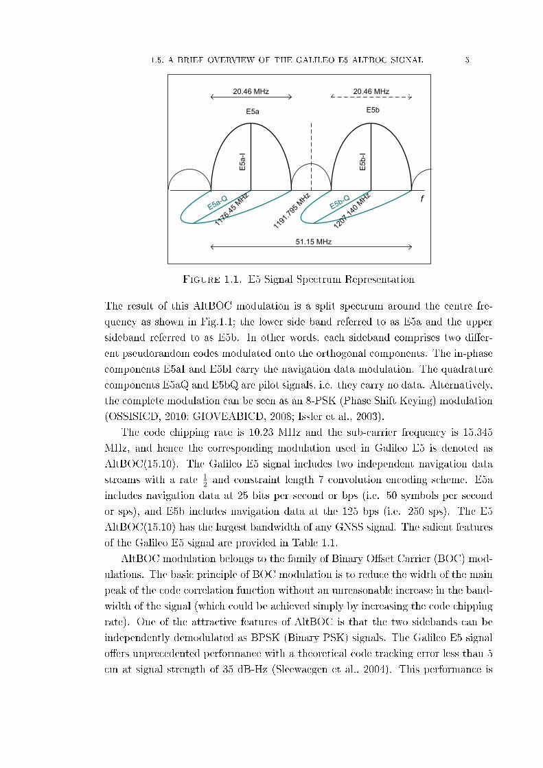
Figure 1.1. E5 Signal Spectrum Representation
The result of this AltBOC modulation is a split spectrum around the centre fre-
quency as shown in Fig.1.1; the lower side band referred to as E5a and the upper
sideband referred to as E5b. In other words, each sideband comprises two di�er-
ent pseudorandom codes modulated onto the orthogonal components. The in-phase
components E5aI and E5bI carry the navigation data modulation. The quadrature
components E5aQ and E5bQ are pilot signals, i.e. they carry no data. Alternatively,
the complete modulation can be seen as an 8-PSK (Phase Shift Keying) modulation
(OSSISICD, 2010; GIOVEABICD, 2008; Issler et al., 2003).
The code chipping rate is 10.23 MHz and the sub-carrier frequency is 15.345
MHz, and hence the corresponding modulation used in Galileo E5 is denoted as
AltBOC(15,10). The Galileo E5 signal includes two independent navigation data
streams with a rate 12and constraint length 7 convolution encoding scheme. E5a
includes navigation data at 25 bits per second or bps (i.e. 50 symbols per second
or sps), and E5b includes navigation data at the 125 bps (i.e. 250 sps). The E5
AltBOC(15,10) has the largest bandwidth of any GNSS signal. The salient features
of the Galileo E5 signal are provided in Table 1.1.
AltBOC modulation belongs to the family of Binary O�set Carrier (BOC) mod-
ulations. The basic principle of BOC modulation is to reduce the width of the main
peak of the code correlation function without an unreasonable increase in the band-
width of the signal (which could be achieved simply by increasing the code chipping
rate). One of the attractive features of AltBOC is that the two sidebands can be
independently demodulated as BPSK (Binary PSK) signals. The Galileo E5 signal
o�ers unprecedented performance with a theoretical code tracking error less than 5
cm at signal strength of 35 dB-Hz (Sleewaegen et al., 2004). This performance is
6 1. INTRODUCTION
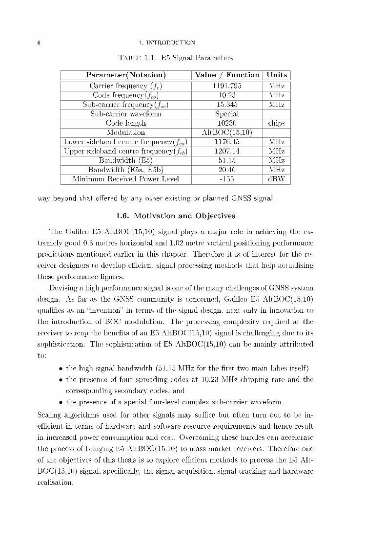
Table 1.1. E5 Signal Parameters
Parameter(Notation) Value / Function Units
Carrier frequency (fc) 1191.795 MHzCode frequency(fco) 10.23 MHz
Sub-carrier frequency(fsc) 15.345 MHzSub-carrier waveform Special
Code length 10230 chipsModulation AltBOC(15,10)
Lower sideband centre frequency(fca) 1176.45 MHzUpper sideband centre frequency(fcb) 1207.14 MHz
Bandwidth (E5) 51.15 MHzBandwidth (E5a, E5b) 20.46 MHz
Minimum Received Power Level -155 dBW
way beyond that o�ered by any other existing or planned GNSS signal.
1.6. Motivation and Objectives
The Galileo E5 AltBOC(15,10) signal plays a major role in achieving the ex-
tremely good 0.8 metres horizontal and 1.02 metre vertical positioning performance
predictions mentioned earlier in this chapter. Therefore it is of interest for the re-
ceiver designers to develop e�cient signal processing methods that help actualising
these performance �gures.
Devising a high performance signal is one of the many challenges of GNSS system
design. As far as the GNSS community is concerned, Galileo E5 AltBOC(15,10)
quali�es as an �invention� in terms of the signal design, next only in innovation to
the introduction of BOC modulation. The processing complexity required at the
receiver to reap the bene�ts of an E5 AltBOC(15,10) signal is challenging due to its
sophistication. The sophistication of E5 AltBOC(15,10) can be mainly attributed
to:
• the high signal bandwidth (51.15 MHz for the �rst two main lobes itself)
• the presence of four spreading codes at 10.23 MHz chipping rate and the
corresponding secondary codes, and
• the presence of a special four-level complex sub-carrier waveform.
Scaling algorithms used for other signals may su�ce but often turn out to be in-
e�cient in terms of hardware and software resource requirements and hence result
in increased power consumption and cost. Overcoming these hurdles can accelerate
the process of bringing E5 AltBOC(15,10) to mass market receivers. Therefore one
of the objectives of this thesis is to explore e�cient methods to process the E5 Alt-
BOC(15,10) signal, speci�cally, the signal acquisition, signal tracking and hardware
realisation.
1.6. MOTIVATION AND OBJECTIVES 7
The E5 AltBOC(15,10) signal encompasses certain unique features that are not
available in other GNSS signals. A non-coherent combination of the individually
processed E5a and E5b correlation outputs produces a BPSK(10)-like correlation
triangle in contrast to the narrow correlation peak obtained by treating the whole
signal as a wideband signal. While a wide correlation peak favours signal acquisition,
the signal tracking errors are generally low for a signal with a narrow correlation
peak. Therefore it is of interest, and a topic in this thesis, to explore signal acquisi-
tion and signal tracking algorithms that utilise the favourable features at each stage
of the signal processing.
The E5a and E5b sidebands can be considered as carrying the same ranging
information (at least the `pilot only' channels) and hence possess the property of
frequency diversity. The e�ect of multipath fading is frequency dependent. One
of the earliest works related to multipath fading and frequency diversity noted the
presence of negative correlation among individual frequency components for di�erent
multipath delays (Haber and Noorchashm 1974). Therefore another topic of interest
in this thesis is to exploit the frequency diversity in order to reduce the e�ect of
multipath on the signal measurements.
A GNSS receiver using the Galileo E5 signal may fall into one of the two cate-
gories, either a standalone Galileo E5 receiver or a multi-band (or multi-frequency)
GNSS receiver where E5 is one of the processed signals. In its simplest form, a
typical civilian multi-band receiver is expected to accommodate the signals in the
L1/E1, L2 and the L5/E5 bands. The Galileo E5a sideband shares frequency spec-
trum with the GPS L5 signal. Moreover, there are several advantages that a receiver
can exploit by using signals from both the E5/L5 and E1/L1 frequency bands, such
as the ionospheric delay estimation and mitigation of RF interference. Therefore,
another objective of this thesis is to study receiver complexity and explore signal
processing algorithms for the E5 AltBOC(15,10) signal in a multi-band receiver, in
addition to those for a standalone E5 receiver.
One of the purposes of having shorter codes in a GNSS is to aid the acquisition
of longer codes in the system, an example being the GPS L1 C/A code aiding the P
code acquisition (Parkinson and Spilker, 1995). However, there is another issue when
the shorter and longer codes are at di�erent frequency bands. If the signal carrying
the shorter code is a�ected due to interference or jamming, the receiver has to spend
its resources searching the entire code delay and carrier frequency ambiguity for the
longer code. Moreover, a receiver has to be designed to handle such worst case
scenarios, which may be an overkill from the system design perspective. To explore
the issue of e�ciently designing core signal acquisition blocks is another aim of this
thesis.
Having discussed the complexity of processing the Galileo E5 AltBOC(15,10)

8 1. INTRODUCTION
signal, it is of interest to examine the signal structure in detail to analyse the un-
derlying contributions to this complexity. Therefore another objective of this thesis
is to explore the possibility of devising a signal that possesses AltBOC-like features,
but reduces the receiver signal processing complexity.
Due to the attractiveness of the AltBOC(15,10) signal, the Chinese naviga-
tion system, COMPASS (a.k.a. Beidou) Phase-III plans to transmit signals called
B2a and B2b that are generated using the AltBOC(15,10) modulation centred at
1191.795 MHz. COMPASS uses the same code chipping rate as the Galileo E5 and
same data rate on B2a as on Galileo E5a (the data rate on B2b is 50 bps/100 sps
instead of the 125 bps/250 sps on Galileo E5b)(Lu, 2010). This supports the view
that most of the receiver algorithms developed for AltBOC(15,10) will eventually
be useful in processing signals from more than one GNSS.
1.7. Contributions
The following are contributions of this thesis:
• A detailed analysis of the Galileo E5 AltBOC(15,10) signal acquisition
strategies, focusing on the acquisition performance and categorisation of
acquisition strategies; studying the signi�cance of cell correlations on the
matched �lter acquisition performance.
• Proposal for a sequential detection acquisition algorithm to acquire sec-
ondary code phase in Galileo receivers.
• Designing a hybrid tracking architecture for the Galileo E5 AltBOC (15,10)
signal that uses a pre-correlation combination method to combine individual
components of the E5 signal with the aim of maximising the received signal
energy.
• Proposal for a novel extended tracking range Delay Locked Loop (DLL)
that combines the bene�ts of BPSK(10) correlation output and wideband
AltBOC(15,10) correlation output, especially for low signal strength and/or
high dynamics applications.
• Design of a mixed-radix Fast Fourier Transform (FFT) architecture that
can be adapted in real-time to perform code acquisition of di�erent GNSS
signals, to eliminate the need for dedicated large-point FFT blocks.
• Evaluation of baseband hardware complexity of multi-band GPS and Galileo
correlators; and estimating the power consumption of modernised GPS and
Galileo receivers.
• A novel (PCT/AU2010/000268) code phase multipath mitigation algorithm
called the Sideband Carrier-Phase Combination (SCPC) method that utilises

1.8. STRUCTURE OF THE THESIS 9
the frequency diversity property of Galileo E5 AltBOC(15,10) to compen-
sate for the group delay at the centre of the E5 band by estimating the
phase delays at E5a and E5b centre frequencies.
• Proposal for a Time-Multiplexed O�set-Carrier Quadrature PSK (TMOC-
QPSK) modulation that resembles a non-constant envelope AltBOC mod-
ulation and TMOC-π4-QPSK modulation scheme that resembles constant
envelope AltBOC modulation, with the proposed modulation schemes re-
quiring reduced complexity at the receiver.
1.8. Structure of the Thesis
The structure of the thesis is depicted in Fig. 1.2.
Chapter 2 provides a detailed description of the Galileo E5 signal structure and
relevant work in the literature concerning the topics dealt within this thesis. The
basics of the Galileo E5 signal structure, acquisition, tracking and multipath are
described here. Context and scope of the topics in this thesis is established and
justi�ed by reviewing the recent work carried out by other researchers.
Chapter 3 discusses Galileo E5 signal acquisition strategies, their performance
and secondary code acquisition. To start with, the probability of detection and
mean acquisition time performances are analysed for the primary code acquisition.
Next, the signi�cance of cell correlations on the acquisition performance is discussed.
Finally, an algorithm to acquire the secondary code phase is proposed.
The �rst part of Chapter 4 discusses hybrid tracking architectures that combine
the correlation outputs of di�erent components of the E5 signal. The second part
proposes a novel way of combining BPSK-like and AltBOC delay locked loops to
obtain an extended tracking range performance for the code tracking.
Chapter 5 explains SCPC, the code phase multipath mitigation algorithm, in de-
tail. A group delay compensation perspective for the proposed multipath mitigation
algorithm is also provided.
The Galileo E5 baseband hardware architecture in the context of a multi-band
(or multi-frequency) and multi-GNSS receiver is described in Chapter 6. First, the
multi-band and multi-GNSS signal processing techniques are categorised. Next, a
novel resource-sharing FFT algorithm is presented and the hardware complexity
results are provided. Finally, the baseband hardware complexity and power con-
sumption of modernised GNSS receivers is analysed.
Chapter 7 introduces the TMOC-QPSK modulation and discusses the bene�ts
that make it attractive as an alternative to AltBOC modulation. Hardware complex-
ity and power consumption estimates of the TMOC-QPSK correlator are compared
to those of an AltBOC correlator.

10 1. INTRODUCTION
Chapter 2Galileo E5 Signal & Related Work
Chapter 3Experimental Setup
Chapter 4Acquisition
Chapter 5Tracking
Chapter 6Multipath Mitigation
Chapter 7Galileo E5 Baseband Hardware
Chapter 8Time-Multiplexed Offset-Carrier
Modulation
Chapter 9Conclusions & Future Work
Chapter 1Introduction (this chapter)
Figure 1.2. Flow diagram showing the thesis structure

1.9. PUBLICATION CROSS REFERENCE MATRIX 11
Chapter 8 concludes the thesis with a summary of recommendations and outlines
some future work.
Appendices A to E provide basic information related to some of the topics dis-
cussed in this thesis. Appendices F to L provide the supporting information required
during the course of development of the methods proposed in this thesis.
1.9. Publication Cross Reference Matrix
The research related to this thesis was conducted between September 2007 and
January 2011. The publication timeline is shown in Fig. 1.3. Publication vs. chapter
cross reference matrix is shown in Table 1.2.

12 1. INTRODUCTION
20
08
20
09
20
10
20
11
Directly related
to the thesisIndirectly related
to the thesis Le
ge
nd
Bla
ck: P
rim
ary
au
tho
r, B
lue
: S
eco
nd
au
tho
r, ☼
IO
N S
tud
en
t P
rize
& S
essio
n’s
be
st
pre
se
nta
tio
n a
wa
rd
Oct
AS
ILO
MA
R
Acq
uis
itio
n
De
c
JG
PS
Mix
ed
-ra
dix
FF
T,
IGN
SS
: A
ltB
OC
Str
uctu
re,
Ce
ll C
orr
ela
tio
n
Ap
r
EN
C L
2C
Acq
uis
itio
n
Au
g
Co
ord
ina
tes M
ag
.
Acq
uis
itio
n
Ma
y
PL
AN
S
Gro
up
De
lay
Se
p
TA
ES
TM
OC
-QP
SK
(Su
bm
itte
d)
No
v
TA
ES
Ce
ll
Co
rre
latio
n
De
c
IGN
SS
FP
GA
Se
arc
h E
ng
ine
Ma
r
Mu
ltip
ath
Pa
ten
t
Se
p
Sta
rt
Ma
y
EN
C H
yb
rid
Tra
ckin
g
Ma
y
ISC
AS
GN
SS
Ba
se
ba
nd
De
c
IGN
SS
Ga
lile
o E
1
FP
GA
Co
rre
lato
r D
esig
n
Se
p
VT
C E
xte
nd
ed
Ra
ng
e D
LL
Ma
y
EN
C F
PG
A
Se
arc
h E
ng
ine
Se
p
ION
L2
C
Ba
se
ba
nd
Ha
rdw
are
Se
p
ION
Se
co
nd
ary
Co
de
Acq
uis
itio
n
Ap
r
EN
C A
cq
uis
itio
n
Str
ate
gie
s
Se
p
ION
Co
de
Mu
ltip
ath
☼M
ar
Th
es
is S
ub
mis
sio
n
Se
p 2
00
7
Ja
n
L1
C H
ard
wa
re C
orr
ela
tor
Ja
n
ITM
: W
ide
ba
nd
Sig
na
l D
esig
n
Figure 1.3. Publication timeline

1.9. PUBLICATION CROSS REFERENCE MATRIX 13
Table 1.2. Publication vs. Chapter cross reference matrix
Publication Chapter/ Section
N. C. Shivaramaiah and A. G. Dempster, An Analysis of GalileoE5 Signal Acquisition Strategies, ENC-GNSS, Toulouse, France,
Apr 2008.
Chapter 4
N. C. Shivaramaiah and A. G. Dempster, Galileo E5 SignalAcquisition Strategies, Coordinates Magazine, vol. IV(8), no. 8,
Aug 2008, pp. 1216,
Chapter 4
N. C. Shivaramaiah, A. G. Dempster, and C. Rizos, Exploiting theSecondary Codes to Improve Signal Acquisition Performance inGalileo Receivers, ION-GNSS, Savannah, GA, Sep. 2008, pp.
1497-1506.
Chapter 4
N. C. Shivaramaiah and A. G. Dempster, An UnambiguousDetector Architecture for Galileo E5 Signal Acquisition, in Signals,
Systems and Computers, Asilomar Conference on, 2008, pp.2076-2080.
Chapter 4
N. C. Shivaramaiah and A. G. Dempster, ProcessingComplex-modulated Signals Involving Spreading Code and
Subcarrier in Ranging Systems, PCT/AU2010/000268, Prioritydate 11 Mar 2009
Chapter6
N. C. Shivaramaiah, A. G. Dempster, and C. Rizos, A HybridTracking Loop Architecture for Galileo E5 Signal, ENC-GNSS,
Naples, Italy, May 2009.
Chapter 5
N. C. Shivaramaiah and A. G. Dempster, A Novel ExtendedTracking Range DLL for AltBOC Signals, in IEEE VTC-FALL,
Anchorage, AK, Sep. 2009.
Chapter 5
N. C. Shivaramaiah, Code Phase Multipath Mitigation byExploiting the Frequency Diversity in Galileo E5 AltBOC, ION
GNSS, Savannah, GA, September 2009.
Chapter6
N. C. Shivaramaiah and A. G. Dempster, Group DelayCompensation in AltBOC Receivers to Mitigate the E�ect ofFrequency Selective Propagation Delay Distortions, IEEE/ION
PLANS, May 2010, pp. 227 235.
Chapter6
N. C. Shivaramaiah, A. G. Dempster, and C. Rizos, Application ofPrime-factor and Mixed-radix FFT Algorithms in Multi-bandGNSS Receivers, Journal of GPS, vol. 8, pp. 174-186, 2009.
Chapter7
N. C. Shivaramaiah and A. G. Dempster, The Galileo E5 AltBOC:Understanding the Signal Structure, IGNSS Symp, Gold Coast,
Australia, Dec 2009.
Chapter2
N. C. Shivaramaiah and A. G. Dempster, Design Challenges of aGalileo E1 Correlator on the Namuru Platform, in IGNSS Symp,
Gold Coast, Australia, Dec 2009.
Chapter7
N. C. Shivaramaiah and A. G. Dempster,Time-Multiplexed-O�set-Carrier Modulations for GNSS, IEEE
Trans. AES (Manuscript Under Review)
Chapter8
14 1. INTRODUCTION
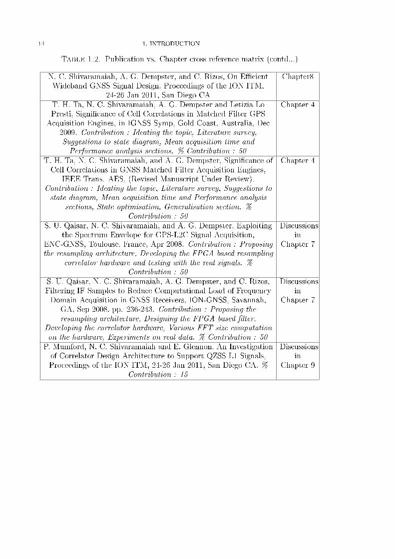
Table 1.2. Publication vs. Chapter cross reference matrix (contd...)
N. C. Shivaramaiah, A. G. Dempster, and C. Rizos, On E�cientWideband GNSS Signal Design, Proceedings of the ION ITM,
24-26 Jan 2011, San Diego CA
Chapter8
T. H. Ta, N. C. Shivaramaiah, A. G. Dempster and Letizia LoPresti, Signi�cance of Cell Correlations in Matched Filter GPS
Acquisition Engines, in IGNSS Symp, Gold Coast, Australia, Dec2009. Contribution : Ideating the topic, Literature survey,Suggestions to state diagram, Mean acquisition time andPerformance analysis sections. % Contribution : 50
Chapter 4
T. H. Ta, N. C. Shivaramaiah, and A. G. Dempster, Signi�cance ofCell Correlations in GNSS Matched Filter Acquisition Engines,
IEEE Trans. AES, (Revised Manuscript Under Review).Contribution : Ideating the topic, Literature survey, Suggestions tostate diagram, Mean acquisition time and Performance analysis
sections, State optimisation, Generalisation section. %Contribution : 50
Chapter 4
S. U. Qaisar, N. C. Shivaramaiah, and A. G. Dempster, Exploitingthe Spectrum Envelope for GPS-L2C Signal Acquisition,
ENC-GNSS, Toulouse, France, Apr 2008. Contribution : Proposingthe resampling architecture, Developing the FPGA based resampling
correlator hardware and testing with the real signals. %Contribution : 50
Discussionsin
Chapter 7
S. U. Qaisar, N. C. Shivaramaiah, A. G. Dempster, and C. Rizos,Filtering IF Samples to Reduce Computational Load of FrequencyDomain Acquisition in GNSS Receivers, ION-GNSS, Savannah,
GA, Sep 2008, pp. 236-243. Contribution : Proposing theresampling architecture, Designing the FPGA based �lter,
Developing the correlator hardware, Various FFT size computationon the hardware, Experiments on real data. % Contribution : 50
Discussionsin
Chapter 7
P. Mumford, N. C. Shivaramaiah and E. Glennon, An Investigationof Correlator Design Architecture to Support QZSS L1 Signals,Proceedings of the ION ITM, 24-26 Jan 2011, San Diego CA. %
Contribution : 15
Discussionsin
Chapter 9

CHAPTER 2
Galileo E5 Signal and the Related Work
2.1. Introduction
This chapter provides the background information required for the rest of the
thesis, including a discussion on relevant previous work. To start with, Global
Navigation Satellite System (GNSS) signal structures are introduced and the Galileo
E5 signal is explained in detail. Next, a brief overview of receiver signal processing is
provided, followed by a detailed discussion of Galileo E5 AltBOC signal processing.
The challenges associated with signal acquisition, tracking, multipath mitigation
and the receiver hardware realisation are discussed in the context of previous work.
The scope of the research work related to this thesis is then established to support
the later chapters.
2.2. GNSS Transmitted Signal structure
Most GNSSs employ the Direct Sequence Spread Spectrum (DS-SS) technique
with all the satellites in the constellation synchronously transmitting navigation sig-
nals. Each satellite is assigned a Pseudo-Random Noise (PRN) spreading sequence
orthogonal (or quasi-orthogonal) to all other PRNs in the system. This technique,
which allows all the satellites to share the same carrier frequency, is the principal
feature of the Code Division Multiple Access (CDMA) technique. The signal energy
of the carrier is spread across a band of frequencies whose bandwidth is determined
by the rate of the PRN sequence, known as the �chipping rate�. In some systems, a
secondary PRN sequence is combined with the assigned PRN spreading sequence (or
primary PRN sequence) to form a tiered spreading sequence. A relatively low-rate
navigation data signal that contains the necessary information to estimate the range
to the satellite, such as time of transmit, satellite orbital parameters and corrections,
is modulated on to the PRN sequence. In general, a GNSS broadcast signal consists
of three components: a radio frequency carrier, a PRN spreading sequence (a.k.a.
ranging code) and the navigation data.
A generic DS-SS CDMAGNSS signal at the transmitter of any particular satellite
at a designated link (or frequency) X can be expressed as:
SX (t) =√
2PT,X < [sX (t) · exp (jωc,X t)] (2.1)
15
16 2. GALILEO E5 SIGNAL AND THE RELATED WORK
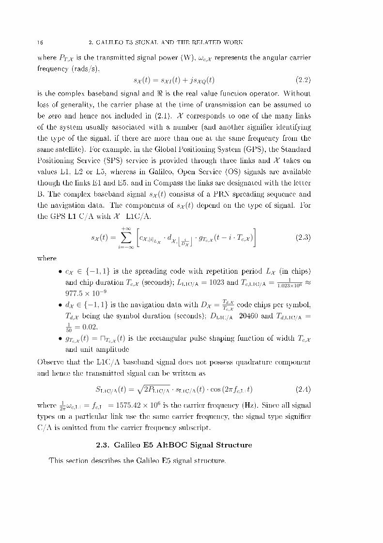
where PT,X is the transmitted signal power (W), ωc,X represents the angular carrier
frequency (rads/s),
sX (t) = sX I(t) + jsXQ(t) (2.2)
is the complex baseband signal and < is the real value function operator. Without
loss of generality, the carrier phase at the time of transmission can be assumed to
be zero and hence not included in (2.1). X corresponds to one of the many links
of the system usually associated with a number (and another signi�er identifying
the type of the signal, if there are more than one at the same frequency from the
same satellite). For example, in the Global Positioning System (GPS), the Standard
Positioning Service (SPS) service is provided through three links and X takes on
values L1, L2 or L5, whereas in Galileo, Open Service (OS) signals are available
though the links E1 and E5, and in Compass the links are designated with the letter
B. The complex baseband signal sX (t) consists of a PRN spreading sequence and
the navigation data. The components of sX (t) depend on the type of signal. For
the GPS L1 C/A with X=L1C/A,
sX (t) =+∞∑i=−∞
[cX ,|i|LX
· dX ,⌊ iDX
⌋ · gTc,X (t− i · Tc,X )
](2.3)
where
• cX ∈ {−1, 1} is the spreading code with repetition period LX (in chips)
and chip duration Tc,X (seconds); LL1C/A = 1023 and Tc,L1C/A = 11.023×10⁶
≈977.5× 10⁻⁹
• dX ∈ {−1, 1} is the navigation data with DX =Td,XTc,X
code chips per symbol,
Td,X being the symbol duration (seconds); DL1C/A=20460 and Td,L1C/A =150
= 0.02.
• gTc,X (t) = uTc,X (t) is the rectangular pulse shaping function of width Tc,X
and unit amplitude
Observe that the L1C/A baseband signal does not possess quadrature component
and hence the transmitted signal can be written as
SL1C/A(t) =√
2PL1C/A · sL1C/A(t) · cos (2πfc,L1t) (2.4)
where 12πωc,L1 = fc,L1 = 1575.42× 106 is the carrier frequency (Hz). Since all signal
types on a particular link use the same carrier frequency, the signal type signi�er
C/A is omitted from the carrier frequency subscript.
2.3. Galileo E5 AltBOC Signal Structure
This section describes the Galileo E5 signal structure.

2.3. GALILEO E5 ALTBOC SIGNAL STRUCTURE 17
2.3.1. The transmitted signal. The Galileo E5 transmitted signal can be
represented as
SE5(t) =√
2PT,E5 < [sE5(t) · exp (jωc,E5t)] (2.5)
Since this thesis deals extensively with the E5 signal, the su�x `E5' is omitted in
future equations and no su�x refers to the E5 signal. Expanding (2.5) and using
(2.2), the transmitted signal can also be written as
S(t) =√
2PT [sI(t) cos(ωct)− sQ(t) sin(ωct)] (2.6)
where ωc= 1191.795 MHz is the centre (carrier) frequency of the E5 signal band
and s(t) = sI(t) + jsQ(t) is the baseband signal.
2.3.2. The baseband signal - constant envelope AltBOC modulation.
The Galileo E5 signal consists of four spreading codes that are modulated onto in-
phase and quadrature-phase components of orthogonal complex sub-carriers. These
phase-points are combined to form a single baseband signal that phase modulates
the carrier according to (2.6). A straightforward way of combining the complex
phase-points is by adding them together. However, such a method results in a non-
constant-envelope baseband signal, i.e. the normalised magnitudes of the resulting
signal do not lie on the unit circle in the complex plane. A detailed description of
the Alternate Linear O�set Carrier (AltLOC) and non-constant-envelope AltBOC
referred to in this thesis as AltBOC-NCE is provided in Appendix A.
In order to avoid the issue of a non-constant-envelope, Ries et al. (2003) proposed
a method wherein the sub-carrier waveforms are modi�ed to obtain a constant en-
velope. (Note: In this thesis, the constant envelope AltBOC is simply referred to as
AltBOC). In this case the sub-carriers are chosen such that the sum and di�erence
of complex values always lie on the unit circle in the complex plane.
The generation of the baseband signal is illustrated in Fig. 2.1.
AltBOC Mux
caI
daI
caQ
cbI
cbQ
dbI
saI
saQ
sbI
sbQ
sE5
Figure 2.1. AltBOC multiplexer illustration

18 2. GALILEO E5 SIGNAL AND THE RELATED WORK
The baseband signal can be represented as (CAB = CosAltBOC):
sCAB(t) =1
2√
2
[(saI(t) + j · saQ(t))
(scs(t)− j · scs(t− Tsc
4))
+
(sbI(t) + j · sbQ(t))(scs(t) + j · scs(t− Tsc
4))
+
(saI(t) + j · saQ(t))(scp(t)− j · scp(t− Tsc
4))
+
(sbI(t) + j · sbQ(t))(scp(t) + j · scp(t− Tsc
4))]
(2.7)
where Tsc = 1fsc
is the period of the sub-carrier. This is the type of modulation used
in the Galileo E5 signal, i.e. s(t) in (2.6) is the same as sCAB(t) (the other type is
SineAltBOC whose linear counterpart is explained in Appendix A).
The de�nitions of the individual components of the baseband signal are provided
in equation form below followed by a brief description:
saI(t) =+∞∑i=−∞
[caI,|i|LaI
· cs,aI,|i|Ls,aI · daI,⌊
iDaI
⌋ · uTc(t− i · Tc)]
(2.8)
saQ(t) =+∞∑i=−∞
[caQ,|i|LaQ
· cs,aQ,|i|Ls,aQ · uTc(t− i · Tc)]
sbI(t) =+∞∑i=−∞
[cbI,|i|LbI
· cs,bI,|i|Ls,bI · dbI,⌊
iDbI
⌋ · uTc(t− i · Tc)]
sbQ(t) =+∞∑i=−∞
[cbQ,|i|LbQ
· cs,bQ,|i|Ls,bQ · uTc(t− i · Tc)]
• sbI(t) is the E5bI signal component (i.e. E5b data signal), saI(t) is the
E5aI signal component (i.e. E5a data signal), sbQ(t) is the E5bQ signal
component (i.e. E5b pilot signal), saI(t) is the E5aQ signal component (i.e.
E5a pilot signal),
• dbI(t) and daI(t) are the data bit modulations of E5b and E5a respectively,
• ex(t) = cx(t) · cs,x(t) is the tiered spreading code, with cx(t) denoting the
primary spreading code of length 10230 with a repetition rate of one mil-
lisecond, cs,x(t) denoting the secondary code of varying length (OSSISICD,
2010) and x denoting the corresponding signal
• LaI , LaQ, LbI , LbQ denote the primary code length (repetition period) in
chips, Ls,aI , Ls,aQ, Ls,bI , Ls,bQ denote the secondary code lengths.
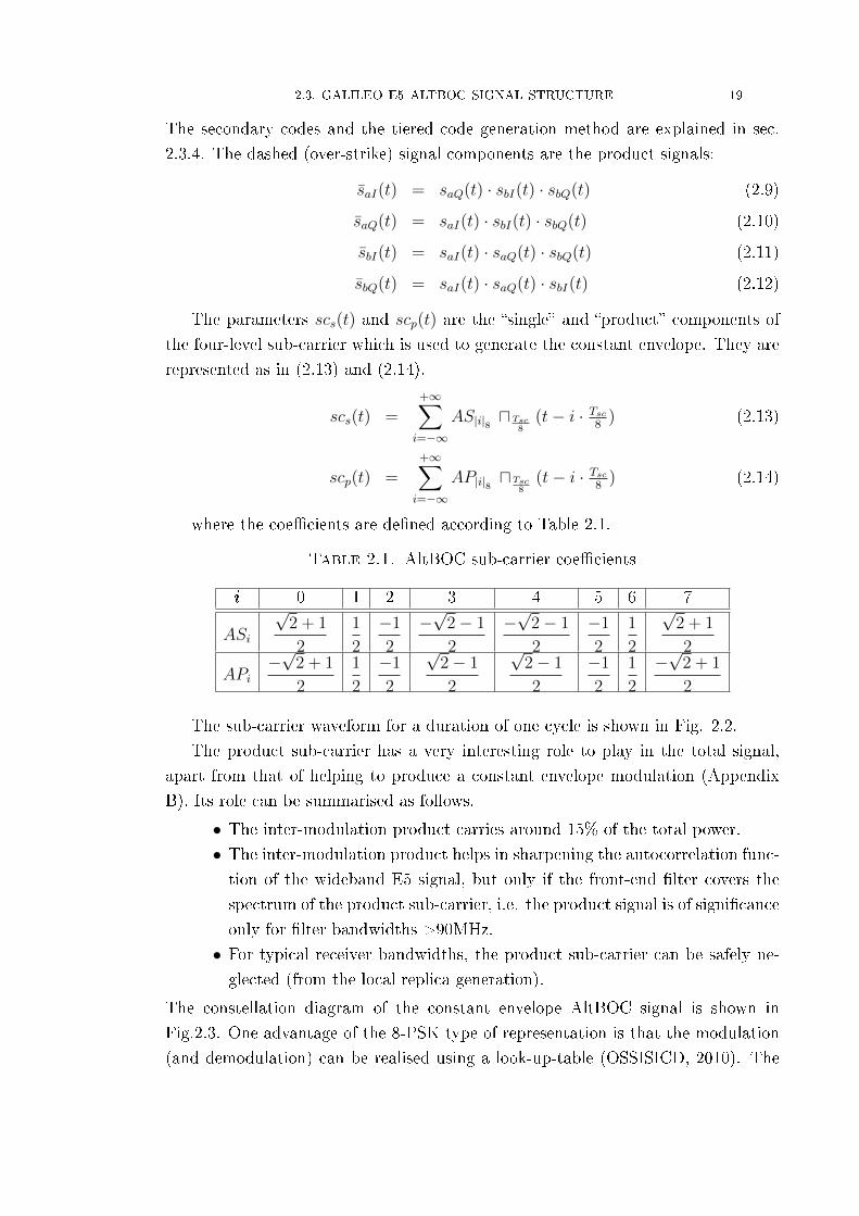
2.3. GALILEO E5 ALTBOC SIGNAL STRUCTURE 19
The secondary codes and the tiered code generation method are explained in sec.
2.3.4. The dashed (over-strike) signal components are the product signals:
saI(t) = saQ(t) · sbI(t) · sbQ(t) (2.9)
saQ(t) = saI(t) · sbI(t) · sbQ(t) (2.10)
sbI(t) = saI(t) · saQ(t) · sbQ(t) (2.11)
sbQ(t) = saI(t) · saQ(t) · sbI(t) (2.12)
The parameters scs(t) and scp(t) are the �single� and �product� components of
the four-level sub-carrier which is used to generate the constant envelope. They are
represented as in (2.13) and (2.14).
scs(t) =+∞∑i=−∞
AS|i|8 uTsc8
(t− i · Tsc8
) (2.13)
scp(t) =+∞∑i=−∞
AP|i|8 uTsc8
(t− i · Tsc8
) (2.14)
where the coe�cients are de�ned according to Table 2.1.
Table 2.1. AltBOC sub-carrier coe�cients
i 0 1 2 3 4 5 6 7
ASi
√2 + 1
2
1
2
−1
2
−√
2− 1
2
−√
2− 1
2
−1
2
1
2
√2 + 1
2
APi−√
2 + 1
2
1
2
−1
2
√2− 1
2
√2− 1
2
−1
2
1
2
−√
2 + 1
2
The sub-carrier waveform for a duration of one cycle is shown in Fig. 2.2.
The product sub-carrier has a very interesting role to play in the total signal,
apart from that of helping to produce a constant envelope modulation (Appendix
B). Its role can be summarised as follows.
• The inter-modulation product carries around 15% of the total power.
• The inter-modulation product helps in sharpening the autocorrelation func-
tion of the wideband E5 signal, but only if the front-end �lter covers the
spectrum of the product sub-carrier, i.e. the product signal is of signi�cance
only for �lter bandwidths >90MHz.
• For typical receiver bandwidths, the product sub-carrier can be safely ne-
glected (from the local replica generation).
The constellation diagram of the constant envelope AltBOC signal is shown in
Fig.2.3. One advantage of the 8-PSK type of representation is that the modulation
(and demodulation) can be realised using a look-up-table (OSSISICD, 2010). The

20 2. GALILEO E5 SIGNAL AND THE RELATED WORK
0 0.125 0.25 0.375 0.5 0.625 0.75 0.875 1−1.5
−1
−0.5
0
0.5
1
1.5
tTsc
Am
plitu
de
scs(t)
scp(t)
−√2−12
−√2+12
Figure 2.2. AltBOC sub-carrier waveforms
Galileo E5 signal uses this constant envelope AltBOC with a sub-carrier frequency
of 15.345 MHz and code chipping rate of 10.23 MHz.
0 1
-j
j
-1
Figure 2.3. Constellation diagram of the constant envelope AltBOCsignal
2.3.3. Nomenclature. The BPSK modulation in GNSS is primarily identi�ed
by associating a number that is related to the primary spreading code chipping
frequency, as in �BPSK(n)�. This number n is simply multiplication factor required
to obtain the chipping frequency relative to 1.023 MHz, i.e. n = fco1.023×106
, fco being
the chipping rate of the signal in question. Hence, the modulation used for GPS
L1 C/A is written as BPSK(1). Another notation PSK-R has also been used in the
literature instead of BPSK, where R stands for �Rectangular� pulse shaping function
whose width is the same as the chip duration. For example, the chipping frequency
used in BPSK(10) modulation (used by the GPS L5 signal) is 10.23 MHz.

2.3. GALILEO E5 ALTBOC SIGNAL STRUCTURE 21
Table 2.2. Galileo E5 OS signal code structure (from (OSSISICD, 2010))
Signal Component Tiered Code Secondary Code Secondary CodePeriod (ms) Length (Chips) Mnemonic
E5aI 20 20 CS201
E5aQ 100 100 CS1001−50
E5bI 4 4 CS41
E5bQ 100 100 CS10051−100
1 2 Lc
1 2 Ls 1
1 2 Lcs
Primary Code
Secondary Code
Tiered Code
1 2 Lc 1 2 Lc 1 2 Lc
1 2
XOR
Figure 2.4. Tiered code generation
The family of BOC modulations have a sub-carrier on top of the spreading code
and are hence identi�ed with two numbers, as in �BOC(m,n)�. In BOC(m,n), n
has the same meaning as given in the previous paragraph and m = fsc1.023×106
, i.e.
it identi�es the sub-carrier frequency as a multiple of 1.023 MHz. For example,
Galileo E1B signal uses a primary code chipping rate of 1.023 MHz and a sub-carrier
frequency of 1.023 MHz, and hence is denoted as BOC(1,1). Another notation
BOC(pn,n) has also been used in the literature instead of BOC(m,n), in which
p = mn
= fscfco
is the ratio of sub-carrier frequency to the chipping rate. AltBOC
modulation also follows this BOC nomenclature and hence the modulation used
for Galileo E5 is AltBOC(15,10). Yet another notation used in the literature is
BOC(fsc, fco) where the arguments are only the ratios with respect to 1.023 MHz,
though they represent actual frequencies. In this thesis, the �rst notation BOC(m,n)
is used unless otherwise speci�ed.
2.3.4. Code length and the generation of tiered codes. All the four pri-
mary codes in the Galileo E5 signal have a length of 10230 chips, i.e. LaI = LaQ =
LbI = LbQ =10230. Secondary codes are multiplied with the primary codes to obtain
the tiered codes. Secondary codes are much shorter in length (i.e. fewer chips) and
much slower (each secondary code chip multiplies one code period of the primary
code).
Table 2.2 details the code structure. Fig. 2.4 illustrates the tiered code gener-
ation. Each chip of the secondary code spans one complete primary code period.
In other words, the chip transition of the secondary code is aligned with the `zero'

22 2. GALILEO E5 SIGNAL AND THE RELATED WORK
point of the primary code. The two codes are XORed to generate the tiered code.
If Lc is the number of chips in the primary code (the length of the primary code)
and Ls is the number of chips in the secondary code, then the tiered code will have
Lcs = Lc · Ls chips.The secondary codes used in Galileo are �memory� codes. Unlike the register
codes that can be generated on-the-�y using shift registers (or a combination of
shift registers), memory codes have to be stored and retrieved for use. The primary
purpose of the secondary codes is to provide better correlation properties for the
�nal pseudorandom sequences without demanding an unreasonably long code delay
search in a receiver. Each secondary code has a code identi�er mnemonic as given
in Table 2.2. For E5aI and E5bI signals, all the satellites use the single secondary
code sequence CS201 and CS41 respectively. For the E5aQ and E5bQ signals, each
satellite has di�erent secondary code sequences (of the same 100-bit length) with
the su�x distinguishing the sequences. Tiered code generation method is explained
in OSSISICD (2010).
2.3.5. The power spectral density (PSD). In order to represent the signal
in the frequency domain, it is required to obtain the power spectral density function
of the signal. The PSD of a constant envelope AltBOC signal is not straightforward
to derive since it involves computing the Fourier Transform of individual pieces of
the sub-carrier waveform. From Rebeyrol et al. (2005); Rebeyrol (2007):
GAltBOC(f) =4
Tcπ2f 2
cos2(πfTc)
cos2(πf Tsc
2
)[cos2
(πf
Tsc2
)− cos
(πf
Tsc2
)− 2cos
(πf
Tsc2
)cos
(πf
Tsc4
)+ 2
],
2fscfco
odd
(2.15)
Equation (2.15) is plotted in Fig. 2.5.
2.4. The Correlation Function
A basic property which enables a receiver to estimate the signal travel time from a
transmitter is the �autocorrelation� property of the spreading code, and the property
that enables CDMA technique to operate in the presence of other signals is the
�cross-correlation� property. Correlation indicates the closeness of match between
two entities, in this context, between two spreading codes. The autocorrelation
function (ACF) of a signal c(t) is de�ned by Braasch and van Dierendonck (1999):
Rc(τ) = limA→∞
1
2A
∫ A
−Ac(t)c(t− τ)dt. (2.16)

2.4. THE CORRELATION FUNCTION 23
−6 −4 −2 0 2 4 6
x 107
−110
−105
−100
−95
−90
−85
−80
−75
−70
−65
−60
frequency (Hz)
Am
plitu
de (
dBW
)
AltBOC − Const. Env.
Figure 2.5. PSD of the constant envelope AltBOC(15,10); zero fre-quency refers to the centre of the band
The autocorrelation of an in�nite random sequence is:
R(τ) = 1− |τ |Tc, for|τ | ≤ Tc
= 0, otherwise (2.17)
where τ is the lag value (in seconds). A truly random sequence is not practical as
it requires in�nite length. In practice, maximal-length sequences (m-sequences or
pseudo-noise sequences) provide a close approximation to random sequences. The
periodic autocorrelation function of an m-sequence of length L is given by:
R(τ) = 1− |τ |Tc
(1
L+ 1
), for|τ | ≤ Tc
= − 1
LforTc ≤ |τ | ≤ (L− 1)Tc (2.18)
The autocorrelation functions of in�nite length and �nite length codes (for the noise-
less case) are shown in Fig. 2.6(Braasch and van Dierendonck, 1999).
GPS L1 C/A signals employ spreading codes known as Gold codes. These codes
are formed by combining two m-sequences. The result is a family of pseudo-noise
codes with low cross-correlation between codes.
A spreading code is said to possesses a good autocorrelation property if the
correlation value for non-zero time lags is a minimum (as close to zero as possible).
Identifying the zero time lag point (the �correlation peak�) is the primary means of
estimating the time delay between the transmitter and the receiver. Since a GNSS
receiver receives combined signals from several visible satellites, the spreading codes
used for di�erent satellites should be distinguishable from each other. In other

24 2. GALILEO E5 SIGNAL AND THE RELATED WORK
1
- T c T c
(a)
1 1
(b)
L -1/L
0
R( )
0
- T c T c
R( )
Figure 2.6. ACF of (a)Truly random sequence, (b)Maximal lengthsequence
words, a set of spreading codes is said to be good if the correlation between any
code sequence in the set with any other code sequence is minimum (as close to zero
as possible) for all time lags.
For BOC(pn, n) signals, the autocorrelation function of the un�ltered signal (p =
1, 2, ...) is given by (Borre et al., 2007; Nunes et al., 2007)
R (τ) =
(−1)k+1[
1p
(−k2 + 2kp+ k − p)− (4p− 2k + 1) |τ |Tc
]|τ | < Tc
0 otherwise(2.19)
where k =⌈2p |τ |
Tc
⌉. Little has been reported in the literature concerning the exact
expression for the autocorrelation function for AltBOC(m,n). However, a very close
approximation is provided in Lohan et al. (2006) as a general expression for Complex
Double-Binary-O�set Carrier (CDBOC) modulations. The equation is repeated here
for AltBOC signals.
R1(τ) =
N1−1∑i=0
N2−1∑k=0
N1−1∑i1=0
N2−1∑k1=0
(−1)i+i1+k+k1ΛTB (τ − (i− i1)TB1 − (k − k1)TB12)
(2.20a)
R2(τ) =
N3−1∑l=0
N4−1∑m=0
N3−1∑l1=0
N4−1∑m1=0
Nres−1∑p=0
Nres−1∑p1=0
(−1)l+l1+m+m1
ΛTB (τ − (l − l1)TB3 − (m−m1)TB34 − (p− p1)TB12) (2.20b)
R(τ) = R1(τ) +R2(τ) (2.20)
where N1 = 3, N2 = 2, N3 = 3, N4 = 1, TBi = Tc/Ni, TBij = Tc/NiNj, Nres =
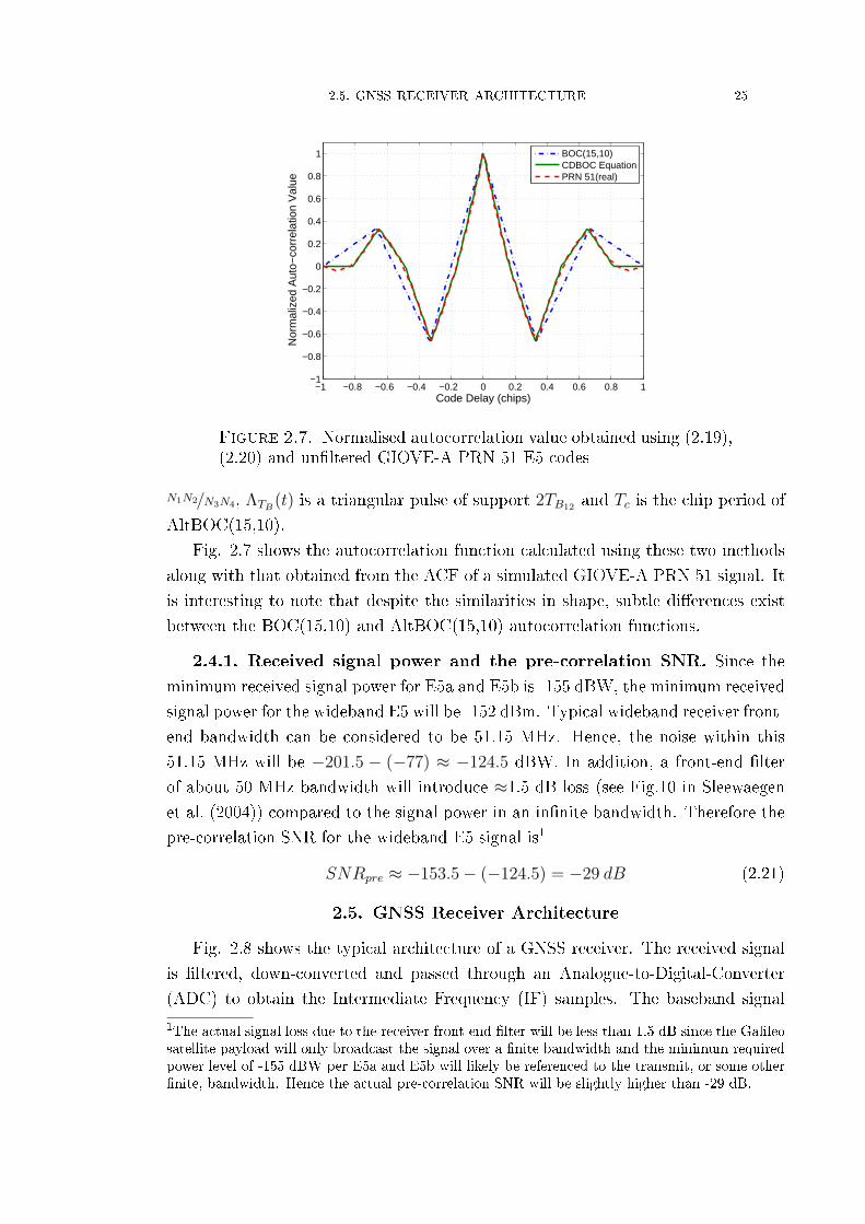
2.5. GNSS RECEIVER ARCHITECTURE 25
−1 −0.8 −0.6 −0.4 −0.2 0 0.2 0.4 0.6 0.8 1−1
−0.8
−0.6
−0.4
−0.2
0
0.2
0.4
0.6
0.8
1
Code Delay (chips)
Nor
mal
ized
Aut
o−co
rrel
atio
n V
alue
BOC(15,10)CDBOC EquationPRN 51(real)
Figure 2.7. Normalised autocorrelation value obtained using (2.19),(2.20) and un�ltered GIOVE-A PRN 51 E5 codes
N1N2/N3N4, ΛTB(t) is a triangular pulse of support 2TB12 and Tc is the chip period of
AltBOC(15,10).
Fig. 2.7 shows the autocorrelation function calculated using these two methods
along with that obtained from the ACF of a simulated GIOVE-A PRN 51 signal. It
is interesting to note that despite the similarities in shape, subtle di�erences exist
between the BOC(15,10) and AltBOC(15,10) autocorrelation functions.
2.4.1. Received signal power and the pre-correlation SNR. Since the
minimum received signal power for E5a and E5b is -155 dBW, the minimum received
signal power for the wideband E5 will be -152 dBm. Typical wideband receiver front-
end bandwidth can be considered to be 51.15 MHz. Hence, the noise within this
51.15 MHz will be −201.5 − (−77) ≈ −124.5 dBW. In addition, a front-end �lter
of about 50 MHz bandwidth will introduce ≈1.5 dB loss (see Fig.10 in Sleewaegen
et al. (2004)) compared to the signal power in an in�nite bandwidth. Therefore the
pre-correlation SNR for the wideband E5 signal is1
SNRpre ≈ −153.5− (−124.5) = −29 dB (2.21)
2.5. GNSS Receiver Architecture
Fig. 2.8 shows the typical architecture of a GNSS receiver. The received signal
is �ltered, down-converted and passed through an Analogue-to-Digital-Converter
(ADC) to obtain the Intermediate Frequency (IF) samples. The baseband signal
1The actual signal loss due to the receiver front-end �lter will be less than 1.5 dB since the Galileosatellite payload will only broadcast the signal over a �nite bandwidth and the minimum requiredpower level of -155 dBW per E5a and E5b will likely be referenced to the transmit, or some other�nite, bandwidth. Hence the actual pre-correlation SNR will be slightly higher than -29 dB.

26 2. GALILEO E5 SIGNAL AND THE RELATED WORK
RF Front end
(Down-
converter +
ADC)
Digital
Baseband
(Correlator)
Processing
(Software)
Antenna
PVT
Solution
Figure 2.8. Typical architecture of a GNSS receiver
processing (widely known as the correlator) is implemented in either hardware or
software, each having its own advantages and disadvantages.
In order to compute the receiver-satellite range and to demodulate the data
streams, a GNSS receiver must �rst synchronise its reference code sequence and
carrier frequency with the satellite signal. To achieve this synchronisation, the
receiver must search for the Doppler frequency and the PRN code chip delay. Signal
synchronisation is generally carried out in two steps: the coarse synchronisation
(referred to as Acquisition), and �ne synchronisation (called Tracking). During
signal acquisition, the receiver searches for available satellites and estimates the
approximate chip delay and Doppler frequency.
The baseband module is responsible for the initial estimation of the time delay
and the Doppler frequency o�set of the received signal with respect to the trans-
mitted signal. With the help of feedback control algorithms (implemented either as
a part of the digital hardware or as a part of the software processing), the base-
band module provides accurate and continuous estimates of the delay, phase and
frequency of the carrier and spreading code in the received signal. The process-
ing, usually implemented in software, computes the position-velocity-time (PVT)
solution corresponding to the phase centre of the receiver antenna. Since the sig-
nal acquisition module is required to search over a range of code delay and carrier
frequencies, both massively parallel time domain correlators and frequency domain
acquisition methods have been used to reduce the search time (Holmes, 2007).
2.6. Signal Acquisition and Tracking: The Basics
The received signal at the IF can be represented as (considering any one satellite)
(Falcone et al., 2006):
rIF (t) =√
2P · < [s(t− τ) · exp (ωIF t+ ωdt+ θ)] + nW (t) (2.22)
where is P the received power (W), ωIF is the intermediate frequency (rads/s),
fd = 12πωd is the Doppler frequency (Hz), θ is the phase of the received signal (rads),
s(t−τ) is the complex baseband signal with a time delay τ (seconds) with respect to
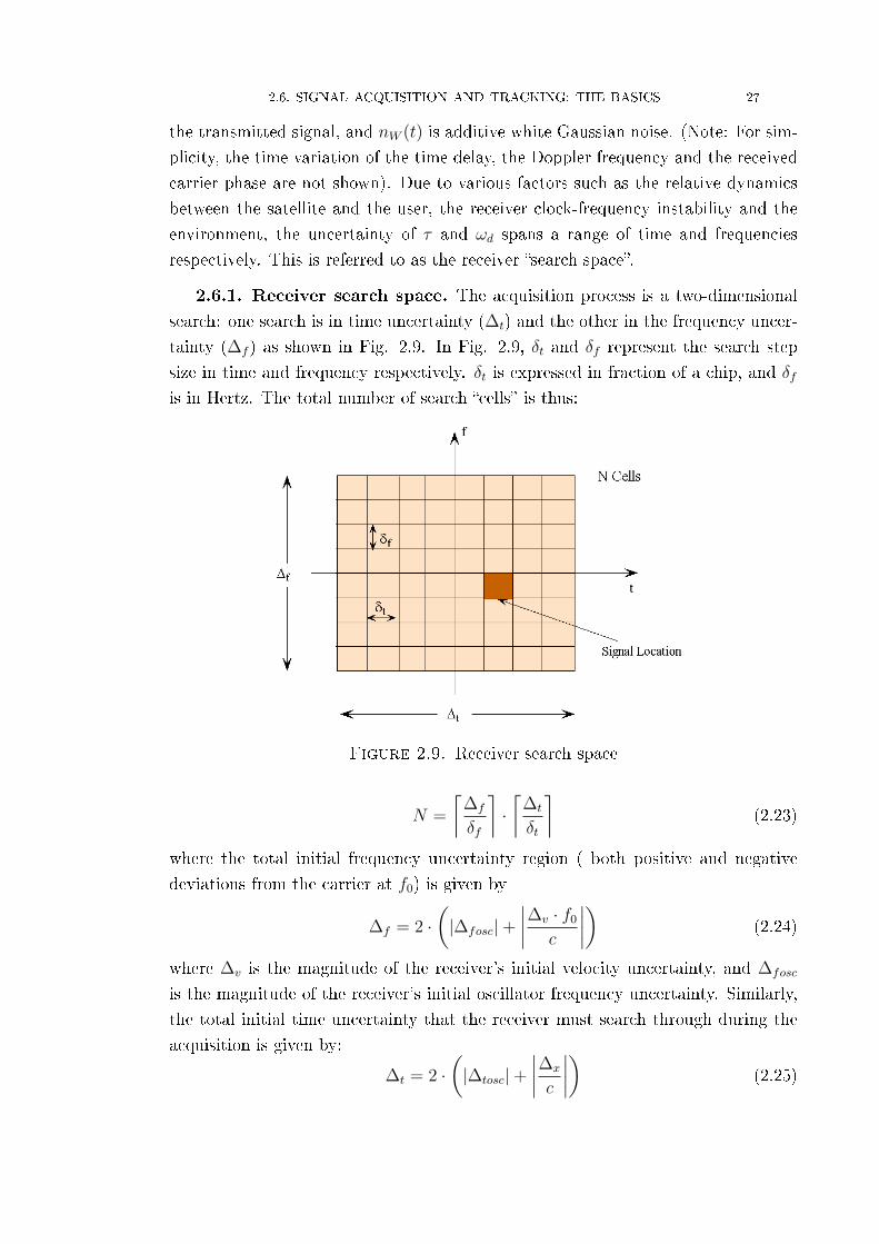
2.6. SIGNAL ACQUISITION AND TRACKING: THE BASICS 27
the transmitted signal, and nW (t) is additive white Gaussian noise. (Note: For sim-
plicity, the time variation of the time delay, the Doppler frequency and the received
carrier phase are not shown). Due to various factors such as the relative dynamics
between the satellite and the user, the receiver clock-frequency instability and the
environment, the uncertainty of τ and ωd spans a range of time and frequencies
respectively. This is referred to as the receiver �search space�.
2.6.1. Receiver search space. The acquisition process is a two-dimensional
search: one search is in time uncertainty (∆t) and the other in the frequency uncer-
tainty (∆f ) as shown in Fig. 2.9. In Fig. 2.9, δt and δf represent the search step
size in time and frequency respectively. δt is expressed in fraction of a chip, and δf
is in Hertz. The total number of search �cells� is thus:
Figure 2.9. Receiver search space
N =
⌈∆f
δf
⌉·⌈
∆t
δt
⌉(2.23)
where the total initial frequency uncertainty region ( both positive and negative
deviations from the carrier at f0) is given by
∆f = 2 ·(|∆fosc|+
∣∣∣∣∆v · f0
c
∣∣∣∣) (2.24)
where ∆v is the magnitude of the receiver's initial velocity uncertainty, and ∆fosc
is the magnitude of the receiver's initial oscillator frequency uncertainty. Similarly,
the total initial time uncertainty that the receiver must search through during the
acquisition is given by:
∆t = 2 ·(|∆tosc|+
∣∣∣∣∆x
c
∣∣∣∣) (2.25)

28 2. GALILEO E5 SIGNAL AND THE RELATED WORK
where ±∆tosc is the receiver's total initial oscillator time uncertainty, and ±∆x is
the receiver's total position uncertainty. Because the code repeats, the maximum
value that ∆t can take is the code length.
2.6.2. The acquisition process. The conventional correlator structure is shown
in Fig. 2.10. The received signal is multiplied by both in-phase and quadrature com-
ponents of the locally generated carrier. The resultant is multiplied with the locally
generated replica signal referenced to a particular time lag. An Integrate and Dump
�lter follows the code mixing for a prede�ned duration MTc. Both in-phase and
quadrature correlation values for a chip shift are then used for envelope detection.
The acquisition decision variable is then compared against a threshold value.
Reference
Generator
Complex
Carrier
c
t
t MT
2
2
To
Tracking( )IFr t
t ct T
[ ]Z n
c
t
t MT
[ ]IX n
[ ]QX n
t ct T
Figure 2.10. Correlator structure for acquisition - conventional scheme
The acquisition decision variable Z[n] is computed as XI [n]2 + XQ[n]2. For the
detection process, the Neyman-Pearson likelihood criterion is used where the Z[n]
is compared with a predetermined threshold η to decide which hypothesis between
H0(Z[n] < η) and H1(Z[n] > η) is true, where
H0: means absence of the desired signal, and
H1: means presence of the desired signal
If Z[n] passes the threshold η (in this situation the receiver time and Doppler fre-
quency estimates are said to be in the H1 region) then a �hit� is declared and the
tracking process is initiated with the approximate time delay and frequency es-
timates. If the acquisition decision variable Z[n] fails to pass the threshold (H0
region), then the code phase of the locally generated code is advanced by δt and
the process is continued until all the cells are evaluated. Several time cells can be
evaluated simultaneously using parallel time domain search techniques or by using
frequency domain correlation methods.
The Integrate and Dump �lter determines the allowable Doppler ambiguity for
detection. For example, an integrate and dump duration of 15.625µs implies a
frequency window of 64 KHz assuming a brick-wall �lter at the zero crossing. The
useful range decreases further because of the sinc nature of the �lter. Depending
on the a priori information about the satellite orbit parameters and the local clock

2.6. SIGNAL ACQUISITION AND TRACKING: THE BASICS 29
Code Delay (chips)
Do
pp
ler
Sh
ift
(kH
z)
Starting cell
x x x
1
|R(t)|2
t (chip)0xx
-1 1-0.5 -0.5
Correct Cell
H0 region
H1 region
-5-4
.5-4
-3.5
-3-2
.5-2
-1.5
-1-0
.50
0.5
11.5
22.5
33.5
44.5
5
0.1
0.2
0.3
0.4
0.5
0.6
0.7
0.8
0.9 1
f (
kH
z)
|sinc(fT
coh)|
2
Threshold
Thre
shold
Figure 2.11. Acquisition output illustration
characteristics, the Doppler ambiguity can range from few kHz (moderately stable
clock) to tens of kHz (for lower stability clock or high relative dynamics scenarios).
Parallel frequency search methods that employ an FFT increase the search speed.
The two-dimensional acquisition output is illustrated in Fig. 2.11 for the case of a
GPS L1 C/A signal, with a random cell as the starting point2.
2.6.3. FFT approach for code correlation. PRN code acquisition in a GNSS
receiver involves correlating the received signal at baseband with all possible time-
delayed versions of the local replica code and searching for the maximum value of
correlation. The correlation value indicates whether proper alignment between the
codes has been achieved. It is well known that the autocorrelation and power spec-
tral density are Fourier Transform pairs and hence time delay searches for the PRN
code alignment can be performed simultaneously for all time delay values using con-
volution according to the Wiener-Kinchine theorem (Proakis and Manolakis, 1995).
The process is to multiply the Fourier Transform of the received signal with the com-
plex conjugate of the Fourier Transform of the local replica code, and then perform
the Inverse Fourier Transform of the product to obtain the result - which is nothing
but a vector of correlation values for all possible time delays. As the sequences are
periodic this can be achieved by making use of FFTs, as has been proposed for GPS
with BPSK signal modulation (Van Nee and Coenen, 1991). Considering a sequence
2Observe that there could be multiple H1 cells during the search as shown in Fig. 2.11.

30 2. GALILEO E5 SIGNAL AND THE RELATED WORK
FFT FFT -1
FFT*
( | |2 )
N-1
∑ ( . )
0
`s(n+m)
Choose
max
Base-band
signal
s(n)
Figure 2.12. FFT method of code acquisition in GNSS receivers
with period L, the autocorrelation in the time domain and via the frequency domain
are given by (Proakis and Manolakis, 1995)
R(m) =L−1∑n=0
s(n) s(n+m) (2.26a)
R = F−1(C(k)C
∗(k))
(2.26b)
where s and s are the received and local code plus sub-carrier, C and C are the
corresponding Discrete Fourier Transforms, and * is the complex conjugate operator.
Fig. 2.12 depicts the code acquisition process using the FFT method. Note that R
is a vector representing the correlation values for each time cell. To decide whether
the proper alignment is achieved between the local code and the code present in
the incoming signal, max(R) is tested against a threshold value. If the local FFT
is stored in memory, only one forward FFT and one inverse FFT operations are
required. It can be seen that the parallel search using FFTs reduces the time required
for code acquisition (Holmes, 2007; Sajabi et al., 2006) by computing the vector R
at once.
2.6.4. Acquisition performance measures. Generally the acquisition per-
formance is measured by two related parameters, the Probability of Detection Pd
(or Detection Probability) and Mean Acquisition Time T acq for a speci�ed Proba-
bility of False Alarm (Pfa), η and the Carrier-to-Noise density C/N0 (Kaplan and
Hegarty, 2006).
The decision statistic for the Direct AltBOC architecture is given by (in the
absence of non-coherent integration)
Z[n] = XI [n]2 +XQ[n]2 (2.27)
Along with the signal components, the output of both the I and the Q channelsXI [n]
and XQ[n] contain noise components nI and nQ and are assumed to be statistically
independent, zero mean, and Gaussian distributed. Also the signal components in
the I and Q channels are assumed to be independent Gaussian distributed random
variables with mean mI and mQ respectively and equal variance of σ2. It has been

2.6. SIGNAL ACQUISITION AND TRACKING: THE BASICS 31
shown (Peterson et al., 1995) that the sum of squares of M independent Gaussian
random variables of the same variance is non-centrally distributed with M degrees
of freedom and with non-centrality parameter3 λ. The non-centrality parameter is
given by
λ2 =M∑i=1
m2i (2.28)
For the Direct AltBOC case, under the hypothesisH0 when there is no signal present,
the decision statistic has a central chi-square distribution with 2 degrees of freedom4
with PDF pn(x) and the Pfa is then given by
Pfa =
∞∫η
pn(x) dx = exp
(−η2σ2
)(2.29)
Under the hypothesis H1 when the signal is present the decision statistic has a
non-central chi-square distribution with 2 degrees of freedom with PDF ps(x) and
non-centrality parameter λ2 = m2I +m2
Q. The Pd is then given by
Pd =
∞∫η
pn(x) dx (2.30)
In order to compute the probabilities, �rst the threshold η for a chosen Pfa is
computed by numerically evaluating the inverse chi-square distribution. Then the
Pd is computed using (2.30) and with the help of the cumulative distribution function
(CDF) of the chi-square distribution (Shnidman, 1989).
Using the probabilities of detection for di�erent received signal strengths and
the probability of false alarm, the mean acquisition time is evaluated. Assuming a
single dwell search the mean acquisition time is given by (Holmes, 1982)
T acq =2 + (2− Pd)(∆t − 1)(1 + kpPfa)
2PdTcohNnc (2.31)
where ∆t is the size of the uncertainty region, kp is the penalty due to false alarm
and Tcoh is the pre-detection coherent integration duration.
2.6.5. The tracking process. For a particular PRN as soon as the presence of
the signal is established and the approximate Doppler frequency and code delay are
estimated, the very next step is to lock onto the signal by more accurately estimating
the Doppler frequency and the code delay. Then the receiver must continuously
3With non-coherent integration, the number of degrees of freedom increases to 2Nnc4The �no signal present� hypothesis modelled using a central chi-squared neglects the possiblepresence of appreciable decision metric amplitude due to cross-correlation with the other PRNs.A more accurate approach to assess acquisition performance uses non-central chi-squared distri-butions for both the �signal present� and �no signal present� hypotheses (see e.g. Appendix B toDierendonck (1996)).

32 2. GALILEO E5 SIGNAL AND THE RELATED WORK
Code Generator
Carrier
Generator
( )IFr t
Code
Loop
Filter
Code
NCO
( )x t
Integrate &
dump
Carrier
Loop
Filter
Carrier
discrimin
ator
Carrier
NCO
Code
discrimin
atorIntegrate &
dump
Integrate &
dump
Early
Late
Prompt
Figure 2.13. Typical tracking architecture; bold lines carry complexvalues
lock onto the signal, or in other words �track�, it in order to generate continuous
carrier Doppler, carrier phase and code phase estimates. Accurate estimation of
these parameters results in accurate estimation of the range measurement. Tracking
the signal is also a requirement to demodulate the navigation data bits transmitted
from the satellites. Signal tracking in GNSS is a vast topic whose fundamentals
are explained in detail in such texts as Parkinson and Spilker (1995); Kaplan and
Hegarty (2006).
As with the acquisition process, the tracking process is also two-dimensional.
Both the carrier frequency and the code delay peaks (the red points in Fig. 2.11)
must be tracked.
A typical tracking architecture is shown in Fig. 2.13. Carrier lock is typically
maintained by employing a Phase-Locked Loop (PLL) or a Frequency-Locked Loop
(FLL) (or a combination of both) whose input is the �Prompt� correlation value
generated by correlating the input signal with the local replica code aligned at the
estimated code delay. Code (delay) lock is maintained by employing a Delay-Locked
Loop (DLL) whose inputs are the correlation values of time shifted, i.e. the �Early�
and the �Late� versions of the local replica code. The code discriminator estimates
the error in the time delay by determining the di�erence in the early and late correla-
tion values, which is then �ltered and provided as a feedback to the code Numerically
Controlled Oscillator (NCO). The code generator then produces the replica codes at
the time delays instructed by the code NCO. The carrier discriminator establishes
the frequency/phase correction required (in terms of frequency or phase depending
on whether it is PLL or FLL) that is �ltered and fed back to the carrier NCO.
When a satellite signal is being continuously tracked, the navigation data bits are
demodulated and measurements are generated. The navigation data bits are used
to extract the time information and compute the satellite position. The satellite
position, time and the phase measurements from the tracking loop are used to

2.7. GALILEO E5 SIGNAL ACQUISITION 33
compute the user position and velocity solution and to estimate any drift in the
receiver clock.
The process of correcting the code delay and the carrier frequency continues as
long as the strength of the received signal is above a point that can be handled by
the tracking loops, and below which the loops cannot generate proper corrections
and the loops lose lock. The loops can also lose lock in other situations such as when
the dynamics of the receiver is beyond the loops' control, or in situations where the
receiver is a�ected by Radio Frequency Interference (RFI), and so on. The ability of
the tracking loops to produce proper corrections is also challenged under multipath
scenarios which distort the shape of the correlation function seen by the receiver.
The performance of the tracking loops depends on several design parameters such
as the type of discriminator used, �lter order, �lter bandwidth and the integration
duration. In general, the performance of the tracking loops is measured in terms
of the standard deviation of the carrier phase error, standard deviation of the code
delay error, the dynamics (velocity, acceleration and jerk) that the loops can handle,
the drift of the clock that the loops can cope up with, and the ability to track weak
signals.
2.7. Galileo E5 Signal Acquisition
The topic of AltBOC(15,10) signal acquisition is interesting due to three reasons.
First, the unique features of the signal, such as independent processing of either the
E5a or E5b side bands or the direct wideband processing, o�er several paths to
estimate the time delay and Doppler frequency of the received signal. Second, the
correlation function of the AltBOC signal resembles those of the BOC modulations,
and therefore the methods developed for the BOC modulation can be explored for
their applicability to AltBOC. Finally, the demand in resources, such as computa-
tional load and the time for acquisition, that basically stem from the fact that the
receiver has to accommodate high bandwidth and four signal components, should
be addressed.
A direct method to process the E5 signal at the receiver is to receive the signal
with at least 51.15 MHz front-end bandwidth and perform the correlation with the
locally generated replica of the modulating signal. This results in a correlation
function as shown in Fig. 2.14.
2.7.1. Autocorrelation waveform of the wideband E5 signal. Fig. 2.15
shows the autocorrelation plot of the wideband E5 signal for di�erent front-end
�lter bandwidths. Observe that even for a 50 MHz �lter, the peak is only slightly
degraded due to the fact that the energy in the two main lobes is still captured with
this bandwidth.

34 2. GALILEO E5 SIGNAL AND THE RELATED WORK
4900 5000 5100 5200 5300−1
−0.8
−0.6
−0.4
−0.2
0
0.2
0.4
0.6
0.8
1
Sample Number
Nor
mal
ized
Aut
ocor
rela
tion
Val
ue
Real ComponentImaginary Component
Figure 2.14. Normalised autocorrelation value of the un�lteredGIOVE-A PRN 51 E5 code with 120 samples per chip and arbitrarychip shift
−1.5 −1 −0.5 0 0.5 1 1.5−0.8
−0.6
−0.4
−0.2
0
0.2
0.4
0.6
0.8
1
Time delay (chips)
Nor
mal
ized
aut
ocor
rela
tion
valu
e
Infinite BW90 MHz70 MHz50 MHz
Figure 2.15. Autocorrelation of the GIOVE-A wideband E5 signal
2.7.2. Correlation function of the components of the E5 signal. In the
receiver signal processing, there may be situations when only a component of the
signal is used. For example, a typical tracking algorithm uses only the pilot signal
or a receiver employing a front-end for GPS L5 (which shares the same main-lobe
frequency range as the E5a signal) may use only E5a component. Fig. 2.16 shows
the correlation waveforms of some components (or combinations of components) of
the E5 signal. Observe that the E5 pilot (combination of E5a and E5b pilot signals)
and the E5 data (combination of E5a and E5b data signals) signals result in similar
correlation waveforms as for the wideband signal. The separate E5a and E5b signals,
being free from the e�ect of sub-carriers, result in single-peak correlation waveforms.

2.7. GALILEO E5 SIGNAL ACQUISITION 35
−1.5 −1 −0.5 0 0.5 1 1.5
−0.5
0
0.5
1E5 Pilot
−1.5 −1 −0.5 0 0.5 1 1.5
−0.5
0
0.5
1E5 Data
−1.5 −1 −0.5 0 0.5 1 1.5
−0.5
0
0.5
1E5a
Nor
mal
ized
cor
rela
tion
valu
e
Time delay (chips)
−1.5 −1 −0.5 0 0.5 1 1.5
−0.5
0
0.5
1E5b
Figure 2.16. Correlation functions of di�erent components of theE5 signal; each waveform is normalised to its own component
2.7.3. Issues with AltBOC(15,10) signal acquisition and the existing
methods. As noted already, the autocorrelation function has side peaks which re-
sult in ambiguous signal acquisition. However, this is not the only issue with Direct
AltBOC acquisition.
First, the required receiver bandwidth to accommodate the two main lobes of
51.15 MHz imposes a limitation on the minimum sampling frequency and is much
higher than that required by other GNSS signals. Typical sampling frequencies
greater than 100 MHz have been used, for example, 122.76 MHz in Dovis et al.
(2007) and 112 MHz in the Septentrio GeNeRx1 receiver, to generate the local
replica and to perform the correlation process. Second, the sharp main peak in the
autocorrelation function restricts increasing the code search step size as is the case
for BOC signals (De Wilde et al., 2006). Third, the side peaks of the autocorrelation
function cause the threat of false transition to the tracking process, unless this is
resolved during the tracking process. Reducing the code search step size increases
the number of cells to be searched during the acquisition.
Di�erent acquisition approaches that exploit independent processing of sidebands
are explained in Martin et al. (2003); Dovis et al. (2007). In the Single Sideband
(SSB) approach, one of the main lobes, either E5a or E5b, is �ltered with a 20.46
MHz �lter and then correlated with respective codes (no sub-carrier is required).
This results in a BPSK(10)-like correlation triangle. In the Dual (or Double) Side-
band (DSB) approach, both the E5a and E5b lobes are �ltered, correlated with
respective codes and combined. Again, this results in a �BPSK(10)-like� correlation
triangle.
The Direct AltBOC acquisition method makes use of the 8-PSK principle and
the local replica can be generated using the look-up table method (OSSISICD, 2010).

36 2. GALILEO E5 SIGNAL AND THE RELATED WORK
In Dovis et al. (2007) a multi-resolution approach to �nd the code delay is demon-
strated. First, coarse acquisition uses the SSB strategy with E5aQ pilot code. With
this the acquisition engine can search at 0.5 chips with a total of 20460 cells for
a one millisecond pre-detection integration. As a second step, �ne estimate of the
code delay is performed with code search step size of 112over 2 chips covering only 24
cells. This reduces the total number of cells searched and also avoids the side peak
ambiguity. However note that in the method proposed in Dovis et al. (2007), the
�rst code delay estimate is going to incur a loss of about 6 dB in Pd (because of only
21% power) compared to the Direct AltBOC processing. In order to compensate for
this loss a minimum of four millisecond pre-detection integration time is required,
which increases the time spent in each cell to 4 ms.
Another class of acquisition technique proposed in the literature addresses the
problem of side peak ambiguity in BOC signals (Heiries et al., 2004; Burian et al.,
2006). These techniques concentrate on the correlation function and try to synthesise
a correlation waveform devoid of any strong side peaks. These techniques hardly
address the correlation loss for larger code search step size scenarios. Some of the
related techniques are:
(1) `BPSK-like' method proposed in Martin et al. (2003) and modi�ed in Burian
et al. (2006)
(2) Sub-carrier Phase Cancellation Method (SPC) proposed in Heiries et al.
(2004)
(3) Very Early + Prompt method mentioned in Heiries et al. (2004)
The `BPSK-like' method essentially falls into the category of the SSB/DSB ap-
proach.
The SPC method is based on the idea of removing the sub-carrier from the
received signal (after carrier removal). In this method, the complex local replica is
generated as in (2.32) where s(t) is the local replica, c(t) is the local code, sc(t) is
the local sub-carrier τ is the delay estimate, and Tsc is the sub-carrier period:
s∗(t− τ) = c(t− τ)
(sc(t− τ)− i · sc
(t− τ − Tsc
4
))(2.32)
As seen from (2.32), the sub-carrier in the quadrature arm of the local replica is
phase-shifted by one quarter of the sub-carrier period. It turns out that when the
BOC signal is multiplied with this local replica the shape of the correlation function
is similar to the BPSK triangle.Fig. 2.17 shows the E5a-Q correlation waveform.
The Very Early + Prompt method, referred here as |V E2 + P 2| works on the
basis that if magnitudes of two correlation values of the BOC signal separated by
an appropriate delay are combined, then it results in a correlation waveform whose
shape is similar to the BPSK triangle. In the |V E2 + P 2| method the local replica

2.7. GALILEO E5 SIGNAL ACQUISITION 37
300 350 400 450 500 550 600 650 700−0.25
−0.2
−0.15
−0.1
−0.05
0
0.05
0.1
0.15
0.2
0.25
Sample number
Nor
mal
ized
Cor
rela
tion
Val
ue
Real
Imaginary
Magnitude
Figure 2.17. Normalised correlation value for E5a-Q code ofGIOVE-A PRN 51
is generated as follows (Heiries et al., 2004):
s∗P (t− τ) = c(t− τ) · sc(t− τ) (2.33a)
s∗V E(t− τ) = c
(t− τ − Tsc
4
)· sc(t− τ − Tsc
4
)(2.33b)
However, the performance of the SPC and the |V E2 + P 2| methods for the Galileo
E5 AltBOC(15,10) signal were not studied in Heiries et al. (2004).
With these discussions it can be observed that there is a need for proper cat-
egorisation, in a broader sense, of the several existing methods. In addition, the
applicability of some of the methods that are not discussed explicitly targeting
AltBOC have to be examined for their feasibility, and the performance of the appli-
cable methods has to be evaluated. For example, in the multi-resolution acquisition
method the feasibility of using the DSB method instead of the SSB method (for the
�rst/coarse search) has to be analysed. A part of Chapter 4 addresses this topic.
2.7.4. The cell-correlation phenomenon. GNSS signal acquisition engines
can be broadly classi�ed into two categories: active correlator and passive matched
�lter (Polydoros and Weber, 1984a,b; Shivaramaiah, 2004). In active correlators,
the local replica code phase is actively self-adjusted to make it compliant with the
incoming code. The dwell time needed to produce a correlation output is equal to
the product between the coherent and noncoherent integration times. However, in
matched �lter (MF) correlators, the local code with a predetermined phase is loaded
into the code bu�er and remains unchanged throughout the acquisition. The MF
just passively waits until the code in the received signal obtains the predetermined
phase. A correlator output is produced whenever a new signal sample arrives in the

38 2. GALILEO E5 SIGNAL AND THE RELATED WORK
Table 2.3. Galileo E1 Open Service signal code structure (from OS-SISICD (2010))
Signal Component Tiered Code Secondary Code Secondary CodePeriod (ms) Length (Chips) Mnemonic
E1B 4 1 -N/A-E1C 100 25 CS251
shift register. This means that the dwell time is just one sample duration, which is
much faster than that of the active correlators.
Due to their attractive acquisition time performance MF correlators promise to
be a good choice for GNSS signal acquisition engines (Holmes, 2007; Lyusin, 1998).
However, consecutive MF correlator outputs are made by the signal segments which
are just di�erent in some samples. Therefore, depending on the sample spacing,
there might exist strong correlations among the consecutive MF correlator outputs.
This e�ect has been studied to some extent for other spread spectrum systems (Sheen
et al., 1999; Giunta and Benedetto, 2007). Existing GNSS signal acquisition methods
that target the design (e.g. threshold determination) and performance evaluation
(detection probability and mean acquisition time), do not consider the e�ect of
cell-correlation. In Chapter 4, a brief description of the e�ect of cell-correlation is
provided (Ta et al., accepted for publication).
2.7.5. Secondary code acquisition. In GNSS, longer integrations are re-
quired to obtain better signal-to-noise ratio during the signal synchronisation pro-
cess. However the presence of secondary codes on the top of primary codes puts a
constraint on the coherent integration duration for pilot channels in a similar way
to the e�ect of data bits in data-carrying channels.
Sec. 2.3.4 described the secondary code structure in Galileo E5. For completeness
Table 2.3 also lists the secondary code characteristics of the Galileo E1 signal. Note
that except for the E1B signal component, which carries only the navigation data,
all the other Galileo OS signals have a two-tiered code structure.
A well known method of weak signal acquisition is to integrate the correlation
values for a longer period in order to achieve a good post-correlation signal-to-noise
ratio, and hence allow a su�cient margin for the decision statistic to pass the acqui-
sition threshold test. Pre-detection integration over one primary code duration is
often not su�cient to acquire weak signals and the presence of a secondary code of
unknown phase prevents the receiver from performing a longer integration. Knowl-
edge of the secondary code phase is required to perform longer coherent integrations.
Extended integration can be achieved by a suitable combination of coherent and
non-coherent integration of the correlation values. Even though the non-coherent
integration performance is inferior to that of coherent integration (Diggelen, 2009),

2.7. GALILEO E5 SIGNAL ACQUISITION 39
it is a preferred choice in traditional receivers so as to integrate across the data bit
boundaries. Secondary codes have the same e�ect on the correlation values as data
bit transitions, but code values are known a priori (but not code phase) by the
receiver, unlike the data.
For a smooth transition from acquisition to tracking it is also necessary to ac-
quire the secondary code chip position. If a receiver employs any of the existing
acquisition methods, then the receiver must follow a two-step procedure: acquire
the primary code �rst and then acquire the secondary code by trying out all the
possible secondary code delays. For longer integrations in weak signal environments
this is a time-consuming task and increases the acquisition time, especially with
long secondary code lengths (such as 100 chips). The other option is to consider
the secondary codes as data bits, in which case the maximum coherent integration
duration during the tracking will be restricted to one primary code period (until the
secondary code phase is determined), which in turn a�ects the tracking performance.
Previous work related to Galileo signal acquisition considers only the primary
code period for coherent integration, and then the result is integrated non-coherently
for longer integration periods, e.g. De Wilde et al. (2006). A closely related work
(Corazza et al., 2007) which uses a multi-hypothesis technique demands larger and
larger memory as the integration time is increased, and in addition the secondary
code phase has to be acquired in a separate process, or one should wait until the
maximum length of the secondary code is reached.
2.7.5.1. Challenges in the presence of secondary codes. In order to reduce the
noise in the acquisition process, a typical method is to integrate the correlation
samples over longer durations so as to reduce the noise bandwidth and hence the
noise at the decision point. Integration for a single period of the primary code may
not yield the required noise performance. For example, the primary codes in E5
signal have a period of one millisecond which o�ers only 30 dB gain in the C/N0,
whereas each doubling this integration time further increases the gain by 3 dB.
Hence in principle, one can keep on increasing the integration time, and for the pilot
signals this process is often only limited by the receiver dynamics and reference
clock frequency drift. In the absence of a secondary code, the integration longer
than one primary code period is performed by coherently combining the successive
correlation samples of one primary code length. This is possible because the primary
code period is only moderately large. On the other hand, the length of the tiered
code is very long, perhaps too long, to be acquired in a single step. Hence the initial
task of the acquisition engine is to align the local primary code replica with the
primary code boundary of the received signal. Once the primary code chip shift
is found, the secondary code chip position is then acquired, thus completing the
acquisition process.

40 2. GALILEO E5 SIGNAL AND THE RELATED WORK
The presence of secondary codes basically imposes two challenges to this process.
The �rst challenge is for longer integration. Because the acquisition engine will not
have knowledge of the secondary code chip position (and hence the chip value),
the secondary code chip transition may result in loss of the coherently combined
correlation value. This problem is similar to the data bit transition problem for
the GPS L1 C/A signal. The simplest solution is to non-coherently combine the
correlation values of one primary code length to obtain the �nal correlation value.
However, the non-coherent combining results in a lower integration gain (mainly
due to the squaring loss). A more sophisticated approach to the longer integration
problem is to analyse the coherent combination of all the secondary code transition
hypotheses and then select the maximum among them. This approach was proposed
earlier in Hegarty (2006) for GPS L5 and later in Corazza et al. (2007). This results
in an evolutionary tree with Ls leaves (where Ls is the number of secondary code
chips) whose size doubles for every additional primary code period, i.e. 2Ls−1, with
the �-1� entering because the receiver does not need to determine the absolute phase
at this stage. For example, in order to integrate for 4 primary code lengths, one
needs to perform and analyse the correlations for 8 di�erent combinations. For 8
primary code lengths integration there will be 128 combinations. It is very di�cult
to handle such high integration durations in practice. Also note that the standard
evolutionary tree approach for the longer integration does not consider the receiver's
knowledge of the secondary code.
The second challenge is to acquire the chip position of the secondary code. It
is necessary to know the secondary chip position so as to pass the information to
the signal tracking stage. Without this information the tracking process can not
�wipe-o�� the e�ect of the secondary code. In the two-step acquisition process, to
acquire the secondary code chip position in E5a-Q or E5b-Q signal, 100 combinations
of 100 consecutive one millisecond correlation values have to be examined. These
two challenges are the main motivations to explore the properties of the Galileo
secondary codes - which is the topic of the secondary code acquisition section in
Chapter 3.
2.8. Galileo E5 Signal Tracking
As with the acquisition, it is possible to track the Galileo E5 AltBOC(15,10)
signal by employing di�erent local reference signals, each focusing on di�erent com-
ponents (or the combination of components) of the signal. The �rst of its kind,
a brief discussion on Galileo E5 AltBOC tracking is provided in Sleewaegen et al.
(2004). The simulation results of tracking with the conventional type architecture
are also provided in Sleewaegen et al. (2004), which is useful in showing the kind of
performance achievable with the AltBOC(15,10) signal.

2.8. GALILEO E5 SIGNAL TRACKING 41
In Soellner and Erhard (2003), the concepts of Central Carrier Single-Sideband-
Tracking (CC-SSB) and O�set Carrier Single-Sideband-Tracking (OC-SSB) are in-
troduced. In CC-SSB the receiver demodulates E5a and E5b signals either by cen-
tring the local carrier frequency at the centre of the respective bands or by translating
the sidebands to the baseband before processing them. In OC-SSB the local carrier
frequency corresponds to the centre of the E5 band, i.e. 1191.795 MHz, and the
sidebands are processed as though they are at an IF of ±15.345 MHz. A tracking
architecture that assists in comparing the performance of Alternate Linear O�set
Carrier (AltLOC) and AltBOC modulation with AltBOC and AltBOC-NCE local
reference signals is presented in Soellner and Erhard (2003). However, Soellner and
Erhard (2003) does not discuss the issue of combining the di�erent components of
the AltBOC(15,10) signal, and also does not discuss increasing the integration du-
ration beyond the data bit boundaries. Depending on whether a receiver transits
to tracking with only the primary code phase estimate or both the primary and
secondary code phase estimates, constraints on the integration duration is imposed,
which in turn a�ects the tracking accuracy. Hence this is an interesting problem to
investigate further.
The general problem of dealing with integration beyond data bit boundaries in
the presence of a pilot and a data signal is not unique to E5 AltBOC. The GPS
L5 signal also consists of a pilot and a data signal component that are in phase
quadrature with each other. In principle, the structure of the Galileo E5a signal,
when considered independently, is similar to the GPS L5 signal structure. Methods
which tackle the problem of data bits can be broadly categorised into post-correlation
combination methods and pre-correlation combination methods.
In post-correlation combination methods, the signal components are combined
after the correlation operation, at the discriminator stage. These methods have
been explored in Hegarty (1999), Tran (2004), Tran (2002) for the GPS L5 and
GPS L2C signals. Basically, a weighted combination of the discriminator outputs
is used to estimate the carrier phase and the code delay corrections within the
tracking loops. These methods can be applied separately to the E5a pilot and
data components denoted here as L(E5aI , E5aQ) and to the E5b pilot and data
components denoted here as L(E5bI , E5bQ). A coherent combination method has
been discussed to improve the signal-to-noise ratio during the acquisition, in the case
of GPS L5 signal acquisition (Yang et al., 2004). The process of linear combination
becomes more di�cult in the presence of two data carrying signals for coherent
integrations more than the symbol duration, which is the situation with the E5
signal.
Some of the architectures in the literature employ the pre-correlation method.
Mattos (2006) proposed a method for combination when there is only one data

42 2. GALILEO E5 SIGNAL AND THE RELATED WORK
component for the Galileo E1 signal. Gerein (2007) proposed a method to demod-
ulate the data by combining reference signals of the data components for the E5
signal. Unlike the post-correlation method, where the correlation for the di�erent
components are obtained independently, pre-correlation methods require a new local
reference signal to be generated.
The challenge of devising an architecture that allows coherent integration longer
than the data bit duration (or the secondary code bit duration) in the presence of
two pilot and two data-carrying components still remains, and is the topic addressed
in Chapter 5. With di�erent architecture modi�cations in context, the e�ect on the
complexity of the pre-correlation combination process in the presence of two data
components is also covered in Chapter 5.
2.8.1. Code lock loop tracking range. The discriminator in the case of a
DLL converts the di�erence in the Early and Late correlation values into the time
delay error (from the correlation main peak) of the Prompt reference signal. The
spacing between the Early and the Late reference signals and the sharpness of the
correlation peak determine the range of time delay errors over which the DLL can
produce corrections so as to �pull� the Prompt to correspond to the peak. Code
tracking linear range and the code phase tracking jitter have always been opposing
design criteria for a code lock loop in GNSS. BOC-type signals o�er better code
tracking jitter and multipath performance by sharpening the correlation triangle.
However the linear tracking range is reduced, which directly results in poor dynamics
and low signal strength performance of the tracking loop. The problem is most
severe in AltBOC modulation, which has the sharpest correlation peak among all
the existing GNSS signals.
The basic principle of the BOC modulations is to reduce the width of the main
peak of the code correlation triangle without an unreasonable increase in the band-
width of the signal (which could be achieved simply by increasing the code chipping
rate). A correlation triangle with a sharp main peak increases the slope of the DLL
discriminator S-curve which in turn results in reduced code phase jitter at the output
of the DLL (Kaplan and Hegarty, 2006). However, the sharpening of the correlation
triangle puts a constraint on the Early-Late correlator chip spacing, and hence the
linear tracking range of the DLL is reduced. While higher dynamics can be handled
by employing a FLL for carrier tracking (Kaplan and Hegarty, 2006), the linear
tracking range of the code lock loop directly a�ects the degree of dynamics that can
be handled and its low signal strength performance. While the e�ect of dynamics
stress on a DLL can be reduced to some extent by carrier Doppler aiding (Kaplan
and Hegarty, 2006), the degraded robustness of the DLL at low signal strength still
remains an issue.

2.9. MULTIPATH MITIGATION IN GALILEO E5 43
Extending the range has been studied in the past (Wilde, 1995, 1998a,b) by
increasing the number of correlator arms and combining their correlation outputs.
These methods are not directly applicable to the BOC family of signals because the
standard Early-Late chip spacing used for BOC signals will already be at the edge of
the linear region, and any additional correlator arm may drive the loop into a false
locking region due to the multiple correlation peaks within one chip. BPSK tracking
can use up to 1 chip as the Early-Late spacing, but till now (Margaria and Dovis,
2008), separate E5a/E5b loops have only been used for the data demodulation with
carrier tracking loops and not for the code phase measurements, so the chip spacing
was of little signi�cance in AltBOC(15,10). The AltBOC modulation technique
can address this problem because it allows the Galileo E5 signal, for example, to
independently process its E5a and E5b components as BPSK signals in addition to
the high performance 8-PSK like main signal. This means that the same satellite
signal can be demodulated to obtain the AltBOC(15,10) correlation function and a
BPSK(10)-like correlation function. Combination of these two types of code tracking
loops is the key point to achieve the extended tracking region discussed in the second
half of Chapter 4.
2.9. Multipath Mitigation in Galileo E5
It is well known that multipath a�ects the performance GNSS. As ways to deal
with other errors progress, the impact of multipath is becoming a more signi�cant
issue. Mitigation of multipath has been a research focus for several decades and the
problem is still persistent (Ward et al., 2006). The research community is trying
to combat multipath fading in two major ways. First, by a signal structure design
approach. Reduction of the e�ects of multipath has been one of the main design
criteria for the newly proposed signals in the GNSS modernisation process (Falcone
et al., 2006). Second, by a receiver design approach. A number of techniques focus
on di�erent stages of the receiver signal processing chain to resolve the e�ect of
multipath on the measurements (Irsigler and Eissfeller, 2003).
Due to the code chipping rate and higher signal bandwidth, AltBOC (15,10) also
helps in eliminating the long-range multipath e�ects on code phase measurements.
However with existing DLL and code discriminator architectures, the short-range
multipath e�ects still remain.
Multipath mitigation via enhanced receiver design methodologies can be broadly
categorised as follows. First, using the Receive Time Diversity (or tapped delay)
techniques and the maximum likelihood principle, the multipath parameters viz. the
attenuation, the multipath delay and multipath phase are estimated. Often, the re-
ceive time diversity has been achieved by employing multiple correlator arms spaced
in time. The Multipath Estimating DLL (MEDLL) (Townsend and Fenton, 1995),
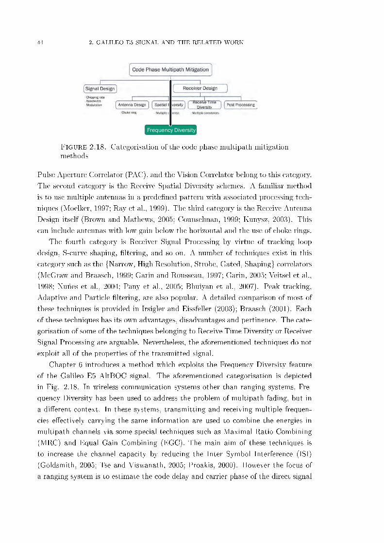
44 2. GALILEO E5 SIGNAL AND THE RELATED WORK
Frequency Diversity
Figure 2.18. Categorisation of the code phase multipath mitigationmethods
Pulse Aperture Correlator (PAC), and the Vision Correlator belong to this category.
The second category is the Receive Spatial Diversity schemes. A familiar method
is to use multiple antennas in a prede�ned pattern with associated processing tech-
niques (Moelker, 1997; Ray et al., 1999). The third category is the Receive Antenna
Design itself (Brown and Mathews, 2005; Counselman, 1999; Kunysz, 2003). This
can include antennas with low gain below the horizontal and the use of choke rings.
The fourth category is Receiver Signal Processing by virtue of tracking loop
design, S-curve shaping, �ltering, and so on. A number of techniques exist in this
category such as the {Narrow, High Resolution, Strobe, Gated, Shaping} correlators
(McGraw and Braasch, 1999; Garin and Rousseau, 1997; Garin, 2005; Veitsel et al.,
1998; Nuñes et al., 2004; Pany et al., 2005; Bhuiyan et al., 2007). Peak tracking,
Adaptive and Particle �ltering, are also popular. A detailed comparison of most of
these techniques is provided in Irsigler and Eissfeller (2003); Braasch (2001). Each
of these techniques has its own advantages, disadvantages and pertinence. The cate-
gorisation of some of the techniques belonging to Receive Time Diversity or Receiver
Signal Processing are arguable. Nevertheless, the aforementioned techniques do not
exploit all of the properties of the transmitted signal.
Chapter 6 introduces a method which exploits the Frequency Diversity feature
of the Galileo E5 AltBOC signal. The aforementioned categorisation is depicted
in Fig. 2.18. In wireless communication systems other than ranging systems, Fre-
quency Diversity has been used to address the problem of multipath fading, but in
a di�erent context. In these systems, transmitting and receiving multiple frequen-
cies e�ectively carrying the same information are used to combine the energies in
multipath channels via some special techniques such as Maximal Ratio Combining
(MRC) and Equal Gain Combining (EGC). The main aim of these techniques is
to increase the channel capacity by reducing the Inter Symbol Interference (ISI)
(Goldsmith, 2005; Tse and Viswanath, 2005; Proakis, 2000). However the focus of
a ranging system is to estimate the code delay and carrier phase of the direct signal

2.9. MULTIPATH MITIGATION IN GALILEO E5 45
excluding all of the superimposed multipath components at the receiving antenna.
As mentioned earlier, the Galileo E5 signal encompasses a number of features.
The two sideband components of the Galileo E5 signal can be considered as car-
rying the same ranging information (at least the `pilot only' channels). The two
sidebands when considered as BPSK(10) di�er in their modulation type to that of
the main signal which is 8-PSK AltBOC (this feature can be argued as being Signal
Diversity - Barnes et al. (2006)). Since the e�ect of multipath fading is frequency
dependent and also depends on the type of modulation, it is of interest to exploit
these features in reducing the multipath e�ect. In addition, one of the earliest works
related to multipath fading and frequency diversity analyses the negative correlation
among the individual frequency components for di�erent multipath delays (Haber
and Noorchashm, 1974). The AltBOC signal exhibits a basic frequency diversity
feature in terms of having a signal transmitted from the same satellite in two di�er-
ent bands, E5a and E5b. The exploitation of these features for multipath mitigation
is the topic of Chapter 5.
Ionospheric e�ects on the wideband signals are discussed in Gao et al. (2007). It
is well known that the ionospheric path is characterised by the direction of arrival,
the wave polarisation, the carrier frequency and the group delay. Only the last two
parameters vary for the E5a and E5b signals. The dispersion within the 51 MHz
band on either side of the E5 centre frequency of 1191.795MHz is nearly symmetric
(Sleewaegen et al., 2004). Even under severe conditions (or storms) of about 100m
ionospheric delay, the di�erence due to the dispersion between E5a and E5b signals
is only 0.33ns. There remains the e�ect of ionosphere dispersion within the useful
bandwidth of 51MHz of the Galileo E5 AltBOC(15,10) signal, but the e�ect due to
the dispersion can be neglected for all practical purposes, as detailed in Sleewaegen
et al. (2004). The second part of Chapter 5 discusses the e�ect of ionosphere on the
multipath mitigation technique that utilises Frequency Diversity.
The e�ect of multipath on group delay has been studied in Otoshi (1993b);
Bishop et al. (1985). Unlike the ionosphere, which directly delays the Line-Of-Sight
(LOS) signal, under multipath conditions the non-LOS (NLOS) (re�ected) signals
are superimposed onto the LOS signal at the receiver antenna. It is of interest to
explore whether the phase at which the NLOS signal is superimposed is di�erent for
E5a and E5b signals, and whether this di�erence follows a pattern, and by combining
the multipath-a�ected carrier phases of the E5a and E5b signals, whether the code
phase multipath error at E5 can be mitigated. Chapter 5 also discusses this group
delay compensation viewpoint.

46 2. GALILEO E5 SIGNAL AND THE RELATED WORK
2.10. Galileo E5 Baseband Hardware
There has been a tremendous increase in interest in satellite-based radio navi-
gation technologies with the announcement of designs for multiple satellite systems
and new ranging signals that will complement those of the venerable GPS. The
greatest interest has been directed to Galileo, as well as the modernisation plans for
GPS. The development of GNSS and Regional Navigation Satellite Systems (Rizos
2007) have posed new challenges to the receiver development community, especially
with regard to the baseband signal processing of multiple GNSS signals (Dempster
2007, Dempster and Hewitson 2007).
As discussed in sec. 2.6.3, due to their fast operation, FFT-based code acquisi-
tion methods are an attractive option for GNSS receiver baseband signal processing
(Van Nee and Coenen, 1991). The requirement for FFT-based code correlation
is more attractive for longer codes, whose acquisition would consume considerable
time if serial code search is employed. However, there are several reasons why the
utility of FFT-based methods is dependent on understanding the trade-o� between
acquisition speed and the required processing power. First, the new signals of the
GNSS family employ longer period PRN codes and higher signal bandwidths, which
demand FFTs of large transform lengths. Secondly, to gain an advantage in posi-
tioning performance, next generation receivers target multiple GNSS signals, and
since each signal has its own code length, the receiver should accommodate FFT
blocks of varying lengths. In a multi-band, multi-system receiver, to handle all the
scenarios including the worst case scenario, i.e. of being able to independently ac-
quire longer codes, the acquisition engine has to be designed to accommodate the
largest FFT required in the system.
An acquisition engine is more useful initially when the receiver is powered on,
rather than during normal operation. Hence the design goal of the acquisition engine
in a multi-band GNSS receiver is to have the �exibility to search any of the desired
signals using as little hardware resource as possible. Though FFT methods speed-up
the acquisition process, this speed-up comes at a cost of increased computational
burden due to the increased FFT length.
There are several schemes to reduce the computational burden by reducing the
number of points required to perform the FFT (see Fig. 2.19).
Acquisition architecture can be modi�ed to realise the correlation with smaller
subsets of the signal and the local code (Yang, 2001; Sajabi et al., 2006), or to
reduce the e�ective transform length (Sajabi et al., 2006; Starzyk and Zhu, 2001;
Qaisar, Shivaramaiah and Dempster, 2008; Qaisar, Shivaramaiah, Dempster and
Rizos, 2008). Another method is to use the assistance data (Diggelen, 2009) from
an external source to narrow down the search space and hence to reduce the size of

2.10. GALILEO E5 BASEBAND HARDWARE 47
Acquisition
Architecture
Modification
Assistance
Information
Reducing the FFT
Computational
Burden
Efficient FFT
Implementation
· External (e.g. AGNSS)
· Internal (e.g. L1 to L5)
e.g.
· Partial Correlation
· Averaging
Figure 2.19. Methods to reduce the FFT computational load
the FFT. This assistance can be from an internal source such as in the case when
the receiver is already tracking a signal at a di�erent frequency band (from the same
satellite) that has shorter code.
In a multi-band GNSS receiver, the receiver has to compute several FFTs of
di�erent sizes due to the varying code lengths of di�erent signals. Hence the receiver
has to accommodate dedicated FFT blocks of varying sizes. Moreover, depending
on the code length and the required chip step, the FFT block requirement may not
always be a power-of-two. For example, a triple-band receiver designed to acquire
GPS L1, Galileo E1, GPS L5 and GPS L2C has to have 2046, 8184, 20460 and
40920 point FFT blocks (half chip step assumed). The transform lengths that are
closer to a power-of-two number can be made power-of-two, by padding zeros (Yang,
2001) and then the power-of-two FFT can be e�ciently computed. In our example
this operation gives 2046 � 2048 and 8184 � 8192. However these techniques do
not solve either the problem of having dedicated FFT blocks of di�erent sizes for
di�erent signals or the problem of having a programmable FFT engine which caters
to all the required transform lengths in the receiver.
Since there are several GNSS modernisation signals with signal structures that
employ di�erent code lengths (apart from the GPS and Galileo civilian signals dis-
cussed in the previous paragraph), having dedicated or individual FFT blocks for
all the signals becomes extremely demanding in terms of the hardware resource and
the computational burden. Chapter 6 proposes methods that fall into a third cat-
egory shown in Fig. 2.19 in which the FFT for a larger set of code lengths (which
includes shorter, moderate and larger codes) is computed e�ciently by a method of
combining the FFT blocks used for shorter code signals.
2.10.1. Resource and power consumption estimate for tracking chan-
nels. Almost all the published work related to the baseband signal processing for
new GNSS signals concentrate on the algorithms, architectures and performance but
do not explore the resource and power requirements from a hardware standpoint.

48 2. GALILEO E5 SIGNAL AND THE RELATED WORK
The large signal bandwidth, multiple longer spreading codes and the split-spectrum
modulations demand wider registers and wider accumulators at higher operating
frequencies compared to the baseband hardware of the existing GPS L1 C/A sig-
nal. Some of the signals with the memory spreading codes have a completely new
requirement of up to 0.5 M memory bits.
Even with the advancement of software receivers, the hardware realisation of the
core correlator channels may become inevitable due to the large number signals that
need to be accommodated (because of multiple signals and multiple systems). A
receiver designed to be capable of processing a multitude of signals faces interest-
ing challenges when it comes to the resource and power consumption requirements
(Dempster, 2007; Dempster and Rizos, 2009). A recent publication McGraw (2010)
also draws attention to the concerns about modernised GNSS receiver baseband sig-
nal processing complexity. In Dempster (2007), it was estimated that a baseband
signal processing module that processes �all� the current and new GNSS signals will
roughly consume 200 times more power than that of a GPS L1 C/A! The contri-
bution of AltBOC(15,10) is the highest among all the other signal types due to its
complexity. In this context, the second part of Chapter 6 analyses the resource
requirement and power consumption of a baseband hardware designed to process
GPS and Galileo civil signals.
2.11. Multiplexing in GNSS Modulations
The GNSS community has paid great attention to signal design during the last
decade, mainly focusing on e�cient spectral utilisation and resistance to propagation
and environmental degradation (e.g. Barker et al., 2000; Betz, Winter 2001-2002;
Betz and Goldstein, 2002; Ries et al., 2002, 2003; Hegarty et al., 2004; Cahn et al.,
2007; Avila-Rodriguez et al., 2008; Stansell, Online).
The major contributors to the AltBOC(15,10) receiver baseband signal process-
ing complexity are the following. First, the receiver must generate four primary
spreading codes and combine them with the secondary codes. An alternative option
is to store the codes in memory. This may not be feasible in all situations (e.g.
if frequency domain techniques are used and FFTs of the local replica are stored)
due to the code length and the number of PRN codes (50 PRNs, four codes each
of 10230 chips length). Second, in the wideband 8-PSK-like processing, the phase
points should be generated using the special sub-carriers that demand accurate rep-
resentation of the sub-carrier amplitude (larger bit-width). Non-constant envelope
AltBOC could be used as an alternative reference signal instead of the constant
envelope AltBOC, but this incurs a loss of up to 1.38 dB (Soellner and Erhard,
2003).

2.11. MULTIPLEXING IN GNSS MODULATIONS 49
The aforementioned points indicate that there exists scope for improvement in
some of the aspects of the AltBOC modulation technique. The tracking and multi-
path performance depend heavily on the RMS bandwidth (or the Gabor bandwidth)
of the signal and hence complexity reduction by reducing the signal bandwidth harms
the performance. However, the signal structure itself can be explored for a speci�ed
signal bandwidth. One such parameter is the way the individual components of the
signal are multiplexed.
AltBOC modulation can be viewed as a method of phase-multiplexing two QPSK
signals. A direct way of phase-multiplexing two QPSK signals disturbs the constant
envelope properties of the signal (Ries et al., 2003). In the constant envelope AltBOC
this issue is resolved by modifying the shape of the sub-carrier waveform and adding
product-signal components. Several signal combining methods have been introduced
in the literature to combine more than one signal component to form a single trans-
mitted signal. These include the Interplex modulation (Butman and Timor, 1972;
Rebeyrol et al., 2006; Fan et al., 2008), Majority Vote combination (Spilker, 1977;
Pratt and Owen, 2005; Rodríguez, 2008) and Phase-Optimized Constant-Envelope
(POCET) combination (Dafesh and Cahn, 2009), which concentrate on the signal
components in a single frequency band. The AltBOC modulation still remains the
best of all the constant envelope phase-multiplexing schemes in the context of four
signal components at two frequency bands (complex sub-carrier), except for the
penalty of receiver complexity required for its demodulation. Time-multiplexing is
another method of combining the individual signal components. Time-multiplexing
has been successfully implemented for two BPSK and BOC signal components in
GPS L2C (ISGPS200E, 2010) and L1C (ISGPS800, 2010). Ries et al. (2002) de-
scribes a time multiplexing method for real sub-carrier BOC signals, but does not
discuss the detailed signal structure and properties, nor the complex sub-carrier
modulation.
Since any improvement in the signal structure is fundamental to the perfor-
mance of the entire system, it is of interest to further explore the time multiplexing
techniques - a topic of Chapter 7.
Apart from the receiver complexity issues, the AltBOC modulation su�ers from
two more drawbacks. First, the AltBOC, with the �rst two main lobes occupying
approximately 20MHz each (for the E5 AltBOC(15,10) example), is more prone to
interference. Second, frequency-selective channel impairments, such as phase delays
due to ionospheric dispersion and multipath, a�ect the signal's performance due to
the higher signal bandwidth. The search for a new signal especially for a wideband
GNSS signal is a very new topic (Mateu et al., 2010). Therefore Chapter 8 also
looks into this topic.

50 2. GALILEO E5 SIGNAL AND THE RELATED WORK
2.12. Summary
This chapter introduced discussions and the earlier work on �ve topics related
to Galileo E5 AltBOC signal viz. signal acquisition, signal tracking, code phase
multipath mitigation, baseband hardware realisation and multiplexing during signal
modulations. During the discussions, important gaps were identi�ed and the scope
for more research work was established. These �ve topics broadly re�ect the contents
of Chapters 4-8.

CHAPTER 3
Experimental Setup
3.1. Introduction
This chapter describes the data acquisition apparatus used to collect Global Nav-
igation Satellite System (GNSS) data required for various experiments conducted
for this thesis. Since this thesis deals with baseband signal processing algorithms,
the type of GNSS data collected is raw Intermediate Frequency (IF) signal samples.
The basic criterion for the experimental setup was to collect the IF samples of the
Galileo E5 and other GNSS signals at least using the same apparatus (except for the
front-end �lters and associated circuitry), if not simultaneously. The data collected
by the data acquisition apparatus was processed in one of the following ways:
• With the help of Matlab software developed by the author; the program
running on a host computer.
• With the help of a Hardware Description Language (HDL) program (Verilog
& VHDL) developed by the author; the program running in simulation
mode in an Electronic Design Automation (EDA) environment (Altera), on
a host computer.
• With the help of a HDL program (as above); the program running on an
Altera Field Programmable Gate Array (FPGA) device, on a hardware
platform.
For simulation studies, signal samples were generated with the help of a Matlab soft-
ware program developed by the author. An overview of the experimental method-
ology is provided in Fig. 3.1. With the data collection apparatus, IF samples were
collected from satellites for GPS L1 C/A, GPS L5 (SVN49), GIOVE-A & GIOVE-B
E1, and GIOVE-A & GIOVE-B E5 signals.
3.2. Data Collection Apparatus
Initially, �nding a data collection apparatus or research platform that can pro-
vide IF signal samples (or at least allow tapping the IF output in a receiver) was a
challenge, especially due to the wideband (>50 MHz) requirement of the Galileo E5
AltBOC(15,10) signal. Fortunately, in the course of this research, four di�erent data
collection apparatus were identi�ed and used as required by the experiments. It is
also worth mentioning here that the reason for using di�erent apparatus was mainly
51

52 3. EXPERIMENTAL SETUP
Signal Generation (MATLAB)
Data Collection Apparatus
Post processing (MATLAB)
IF Samples
Results
Host Computer Host Computer
Post processing (EDA Environment)
Host Computer
Storage (file)
Results
Post processing (FPGA Device)
FPGA Board Results
Host Computer
Hardware Setup
Antenna
OR
OR
OR
FPGA output capture
Host Computer
Signal Generation / Collection
Baseband Algorithms Implementation
Software Components
Hardware / HDL / Firmware Components
Figure 3.1. Overview of the simulation / experimental setup
because each setup had its own limitations. This section provides an overview of
these data collection apparatuses. The following items are discussed for each setup:
block diagram or picture, GPS / Galileo civil signals accommodated, bandwidth,
sampling frequency, number of Analogue-to-Digital-Converter (ADC) bits per sam-
ple (or number of processed bits per sample), limitations of the setup, antennas
used, and usage instances in this thesis.
3.2.1. Septentrio GeNeRx1. The GeNeRx1 is a multi-frequency GPS/Galileo
receiver developed by Septentrio (Septentrio, 2006). GeNeRx1 allows logging of IF
signal samples to a host computer via an Ethernet link. Though GeNeRx1 is capable
of simultaneously processing GPS and Galileo signals at di�erent frequency bands
as a receiver, IF logging is possible for only one frequency band at a time. The GPS
Galileo L1/E1 band is down-converted to an IF of 140.12 MHz with a bandwidth
of 40 MHz. The GPS L5 / Galileo E5 has an IF of 139.905 MHz with a bandwidth
of 55 MHz. The sampling frequency for all the signals is 112 MHz. Quantisation is
8-bits / sample. The front-end used for the GPS L2 signal has a bandwidth of 25
MHz, but IF sample logging is not allowed. The GeNeRx1 receiver is shown in Fig.
3.2. A Leica AR25 antenna (Bedford et al., 2009) was used to collect the signals.
Advantages
• Wide bandwidth (55 MHz) to capture the Galileo E5 AltBOC(15,10) signal.
• Accessibility - this setup was located at the UNSW Satellite Positioning and
Navigation (SNAP) Lab and hence it was available for data collection most
of the time (GeNeRx1 was also being used by the German Aerospace (DLR)
for GIOVE-A/B orbit monitoring), from Feb 2008 through Dec 2010.
Limitations

3.2. DATA COLLECTION APPARATUS 53
Figure 3.2. GeNeRx1 receiver
• Maximum data collection size is 16MBytes and hence the maximum dura-
tion of continuous IF data that can be captured is 149.79 ms.
� This is not an issue for signal acquisition since one primary code period
of Galileo E5 signal is one millisecond and the maximum length of the
secondary code is 100 (which results in a 100 ms tiered code period).
Therefore the signal of length one tiered code period can be easily
observed. However, when the acquisition module passes the estimates
to the tracking module, tracking loops may not settle within 149 ms and
hence it is di�cult to measure the tracking performance. This problem
was addressed to some extent by improving the estimates provided
to the tracking module (�ne synchronisation) to help the loops settle
within the �rst 50 ms (say) or less.
• Either the signal from the L1/E1 band or the L5/E5 band can be captured
in one stretch (but not both simultaneously), and hence no dual-frequency
algorithms can use the data collected with this setup.
• The GeNeRx1 receiver operation halts during the IF sample download op-
eration. Hence permission from the DLR was required every time logging
of the IF samples was attempted.
Due to the third limitation no performance comparison was possible on the same
dataset with respect to the baseband algorithms running inside the GeNeRx1 re-
ceiver. However, the carrier Doppler and the signal strength output of the acquisition
algorithms/tracking developed by the author were found to agree with those pro-
vided by the GeNeRx1 receiver (observed a few seconds before and after the data

54 3. EXPERIMENTAL SETUP
USRP2
Antenna
GNU Radio capturing the
samples
Host Computer
Figure 3.3. USRP2 data collection setup
collection).
3.2.2. Universal software radio peripheral (USRP / USRP2) with
GNU radio. The USRP, developed by Ettus Research LLC, is a family of gen-
eral purpose platforms for software-de�ned radios (SDR)(Ettus, 2010). GNU Radio
is an open-source SDR platform. The USRP product family consists of the mother-
boards, which contain an FPGA for high speed signal processing, and interchange-
able daughterboards that cover di�erent frequency ranges. Together they provide a
�bridge� between the host computer and one or more antennas.
USRP is the �rst generation motherboard, and USRP2 is the second generation
motherboard. The maximum possible bandwidth in USRP is 16 MHz, and for
USRP2 it is 50 MHz; IF being zero in both cases. However the USRP2 �rmware and
the GNU radio software currently do not support more than 25 MHz bandwidth and,
in addition, the data collection at bandwidths 20 MHz and beyond are unreliable
(frequent loss of samples).
The daughterboards that cover the GNSS bands are1 DBSRX(800 MHz to 2.4
GHz receiver), RFX1200 (1150-1450 MHz transceiver) and RFX1800 (1.5-2.1 GHz
transceiver). Initial evaluation showed that the RFX1200 and RFX1800 were slightly
better (about 1.5 dB) in signal strength than the DBSRX boards, and also in terms
of having fewer spurious frequency components in the collected signal spectrum.
The USRP2 setup is shown in Fig. 3.3.
Two antennas were used for the data collection: the Leica AR25 which was
on the roof-top of the Electrical Engineering building at UNSW and the Antcom
2GNSSA-XMNS-1(Antcom, 2010).
Advantages
• Portability - extremely easy to carry around to collect IF samples, especially
USRP2 and the Antcom 2GNSSA antenna1WBX (50 MHz to 2.2 GHz transceiver) is a recent addition and was not available when theexperiments were carried out

3.2. DATA COLLECTION APPARATUS 55
Averna record & playback
systemLNA
40 dB pre-amp
Roof-top antenna
Figure 3.4. Averna setup
• Accessibility - always available, UNSW SNAP Lab has several USRP2
motherboards and daughterboards
Limitations
• 50 MHz wideband signal could not be captured with a single USRP2.
� USRP2 boards are designed to be used in a Multiple-Input-Multiple-
Output (MIMO) setup, in a master-slave arrangement, and one should
be able to coherently sample and capture two 20 MHz wide E5a and
E5b bands. However this arrangement had other issues, such as using
the external clock in the slave and synchronising the bits transferred
from two di�erent boards.
• IF signal capture at 20 MHz for longer durations (longer than about 2
seconds) is unreliable (discontinuities in the sample collection).
The data collected from the USRP2 was useful in observing the GPS L5 and Galileo
E5a signals together for a duration longer than 150 ms (which was not possible with
GeNeRx1).
3.2.3. Averna / National Instruments (NI) record & playback system
at University of Colorado, Boulder (UCB). During the �nal stages of the
research, the wideband Galileo E5 signal samples of longer duration were collected
with the aid of an Averna / NI record and playback system available in the GNSS
Lab at the UCB Aerospace Engineering department. A/Prof. Dennis Akos provided
data �les and also accommodated the author in the GNSS Lab for a short duration
to collect additional data.
The Averna record and playback system is built on NI's PXI Express architecture.
The captured data is streamed in real time to a high capacity RAID system. The
Averna system at UCB can capture data up to a bandwidth of 50 MHz, and can
cover all the GNSS frequency bands. LabView-based software in the host computer
helps control di�erent parameters such as the bandwidth/sampling frequency, gain,
etc. The Averna setup is shown in Fig. 3.4. Several datasets were collected using
two types of antennas: a NovAtel 704-X(NovAtel, 2010) and an Antcom 42GNSSA-
XT-1(Antcom, 2010). Datasets collected using the NovAtel antenna were found to

56 3. EXPERIMENTAL SETUP
be better (in signal strength at the output of the correlator, tested with the help of
an SBAS satellite) than the Antcom antenna. The IF was zero and the sampling
frequency was 62.5 MHz. The 16-bit ADC output was re-quantised to 8-bit / sample.
A dataset was also collected by Dr. Akos, using an 18 m parabolic dish antenna
situated about 40 miles from UCB.
Advantages
• This setup allowed capture of wideband (50 MHz) IF signal samples for
longer durations (a few minutes)
• One of the datasets collected using the 18 m dish was helpful in obtaining
the GIOVE-B signal with a high Carrier to Noise density (C/N0)
Limitations
• High DME/TACAN interference was experienced within the E5 band in
Boulder. The area surrounding Boulder has a high density of VOR-DME /
TACAN stations and, as a result, signal strength degradation of 10-14 dB
was observed at the output of the correlator. Therefore only some of the
datasets collected using this setup could be used2.
• A di�erence in signal strengths of about 2-3 dB between the E5a and E5b
bands were observed, even with the 18 m parabolic antenna and, the source
of this error could not be established (the processing software used to de-
termine this di�erence was the same as that used with the GeNeRx1 setup,
except for the modi�cations in sampling frequency and IF values).
• Not being available at the UNSW SNAP Lab, opportunities to use it were
limited.
3.2.4. Transform-domain instrumentation GPS Receiver (TRIGR) plat-
form from Ohio University (OU). The information related to TRIGR and the
pictures included here were provided by Dr. Sanjeev Gunawardena of the Ohio Uni-
versity Avionics Engineering Center. Dr. Gunawardena also collected the IF samples
when the GIOVE-A or GIOVE-B satellites were visible over Athens, as requested
by the author. This setup was used during the �nal stages of the research3.
TRIGR is a GNSS receiver platform developed by the Ohio University Avionics
Engineering Center, which can be used to collect data from up to 8 front-end modules
with a maximum continuous data streaming rate (to disk) of about 250 MB/sec.
The maximum bandwidth possible for each front-end channel is 24 MHz. The raw
2The signals could be used with the pulse blanking technique, but the experiments in this thesisfocused on the signals without DME/TACAN interference for most of the tests, to match theprocess followed with other setups.3TRIGR was initially capable of collecting data in the L1, L2 and L5/E5a bands. Upon an enquiryby the author, Dr. Gunawardena agreed to include the E5b capability.

3.2. DATA COLLECTION APPARATUS 57
Front-End Architecture
Active
Splitter
Networks
or
Direct
Connect
to
Antennas
-11.5 to 20 dB
DVGA2
PLOfLO1 =
fc-70 MHz
LPFRF-BPF IF-BPF
DVGA1
-11.5 to 20 dB
GNSS Front-End Module
PLO
High Speed
Serial LVDS
Interface
to
Data
Collection
Server
ADC4 or 8 Ch
12-bit
65 MSPS
max
CH_A
Enc
Ant. Feeds
OCXO
SPI
Interface
ADC
Control
10 MHz Reference Osc.
(Internal or External)
CH_BGNSS Front-End Module fc: any, BW: 20-24 MHz
fs = 56.32 MHz
RF/IF Digital
Gain ControlSPI Interface
CH_CGNSS Front-End Module fc: any, BW: 20-24 MHz
CH_DGNSS Front-End Module fc: any, BW: 20-24 MHz
Figure 3.5. TRIGR front-end architecture
GPS L1, L2, L5or custom GNSSRF Front-EndModules
4-Channel or 8-Channel
Coherent Sampling Module
Active Signal SplittersIncluding Antenna Power
High-SpeedLVDS Datalink toData Collection Computer
GNSS Front-End Unit (top)
Figure 3.6. TRIGR GNSS front-end unit
data from the ADC is sent to an FPGA processor inside the server unit via a high-
speed serial interface. The FPGA packs the channels into a 32-bit format which is
then DMA (Direct Memory Access) transferred (via 8x PCI-Express) to the server
and written to an 8-disk RAID array. Depending on the packing format selected,
the 250 MB/sec data rate may contain up to any two channels at 16-bits/sample or
8 channels at 4-bits/sample. Fig. 3.5 shows the TRIGR front-end architecture and
Fig. 3.6 shows the TRIGR unit itself .
The IF samples were collected using a NovAtel GPS-740x antenna with a ~40 dB
gain <1 dB noise �gure Low Noise Ampli�er (LNA). The frequency bands covered
were GPS L1 / Galileo E1 (20 MHz), GPS L2 (20 MHz), GPS L5 / Galileo E5a
(24 MHz), and Galileo E5b (24 MHz). The sampling frequency was 56.32 MHz,

58 3. EXPERIMENTAL SETUP
with IF centred at 13.68 MHz for L1 and L2 signals, 14.13 MHz for L5/E5a signals
and 13.82 MHz for the E5b signal. The number of quantised bits were modi�ed to
2-bits/sample to reduce the �le size (since a lot of data �les were transferred via
FTP).
Advantages
• This setup allowed capture of the civil signals with 20 MHz bandwidth in
L1/E1, L2, L5/E5a and E5b bands simultaneously for longer durations (a
few minutes).
Limitations
• Initial tests showed a slight di�erence in the signal strengths received by
the E5a channel and the E5b channel for both GIOVE-A and GIOVE-B
signals. Since the transmission correctness of the GIOVE-A and GIOVE-B
test satellites could not be established, the source of the problem could not
be identi�ed. Hence this data was not used for the tests on algorithms that
required E5a and E5b signal strength comparison.
• Not being available at the UNSW SNAP Lab, opportunities to use it were
limited.
3.3. Summary
Matlab-based software was developed by the author to acquire and track the
Galileo E5 signal, along with GPS L1 C/A, GPS L2, GPS L5 and Galileo E1 signals.
The Matlab-based software was veri�ed with the aid of IF signals captured using
the GeNeRx1 receiver.
The Verilog-based baseband hardware components (the core correlator modules)
were developed by the author for the Galileo E5 signal. The functionality of the
correlator modules were veri�ed with the aid of EDA simulation tools and the data
captured using the GeNeRx1 receiver.
Due to the 150 ms signal capture duration limitation of the GeNeRx1 setup,
other data collection apparatus viz., the USRP setup, the Averna setup and the
TRIGR setup were identi�ed and examined for their usability, though the last two
setups were used only during the �nal stages of the research. The advantages of each
experimental setup were applied in order to test some of the algorithms developed
during this research.
This exercise not only helped in obtaining some useful datasets for the experi-
ments conducted during the research, but also helped identify some limitations in
these setups (and any other similar experimental setup). Some of the datasets that
could not be used for the experiments in this thesis - and in fact pose di�erent sets

3.3. SUMMARY 59
of challenges, that would be experienced by other researchers while processing E5
signals - is an interesting topic to address in future work.


CHAPTER 4
Galileo E5 Signal Acquisition
4.1. Introduction
This chapter covers the topics related to the Galileo E5 primary code and sec-
ondary code acquisition identi�ed in Chapter 2. Sections 4.2, 4.3 and 4.5 contain
the work published in ENC-GNSS 2008 (Shivaramaiah and Dempster, 2008a); sec.
4.4 contains a part of the work accepted for publication in IEEE TAES (Ta et al.,
accepted for publication); sec. 4.6 contains the work published in ASILOMAR 2008
(Shivaramaiah and Dempster, 2008b), and sec. 4.7 contains the work published in
ION GNSS 2008 (Shivaramaiah et al., 2008).
The contributions of this chapter are:
• categorisation of the existing Galileo E5 AltBOC acquisition methods,
• analysis of the e�ect of code search step size on AltBOC(15,10) signal ac-
quisition,
• examining the e�ect of cell correlation in Global Navigation Satellite System
(GNSS) matched �lter (MF) receivers and discussing the importance of its
inclusion in the acquisition performance analysis,
• analysing the performance of the |V E2 + P 2| method for AltBOC(15,10),
• analysing the correlation properties of secondary codes used in GPS L5,
Galileo E1 and Galileo E5,
• de�ning and describing the �characteristic length� property of secondary
codes used in GNSS, and
• proposing a sequential method (based on the principles of convolutional
decoding) to acquire the secondary code phase
This chapter is organised as follows: Sec. 4.2 details the di�erent signal acquisition
strategies; sec. 4.3 discusses the acquisition complexity followed by a description of
the e�ect of cell correlation phenomenon in sec. 4.4; sec. 4.5 analyse the performance
of the |V E2 + P 2| method. Sec. 4.6 revisits the |V E2 + P 2| method in the presence
of �ltering and the type of decision methodology. Sec. 4.7 describes the properties
of secondary codes and proposes a method to acquire the secondary code phase.
Sec. 4.8 summarises the �ndings of this chapter.
61

62 4. GALILEO E5 SIGNAL ACQUISITION
4.2. Galileo E5 Acquisition Strategies
4.2.1. Categorisation of the acquisition methods. The acquisition perfor-
mance parameters Pd and T acq are directly and inversely proportional respectively,
to the signal-to-noise-ratio (SNR) of the desired signal. The code length and the au-
tocorrelation properties of the ranging code, granularity of time and frequency steps
and the search strategy all in�uence the Pd and T acq for a speci�ed Pfa. BPSK
modulated ranging codes o�er triangular autocorrelation function (ACF) with a
single main peak which, in most situations provides a good Pd and T acq for half-chip
search steps. However, as seen in Chapter 2, BOC and AltBOC modulations pro-
duce multiple peaks in the ACF which create ambiguities during acquisition, and
require better processing to achieve Pd and T acq comparable to that of GPS L1 C/A
under similar conditions.
The principal aim of any acquisition method in GNSS is to address the issue of
e�ciently achieving the required Pd and T acq. Though Pd and T acq are inter-related,
the methods discussed in Chapter 2 can be broadly classi�ed into two groups, one
which primarily targets Pd and the other that primarily addresses T acq.
�Search strategy� based methods. The methods which target T acq basically try
to avoid acquiring the narrow correlation peak since such a narrow peak demands
smaller search steps1. For example, by correlating the two sidebands independently
acquisition engines obtain a correlation waveform without multiple peaks. This al-
lows the acquisition engine to increase the code search step size (or equivalently
reduce the number of search cells).In other words, these methods look for a di�er-
ent search strategy and can be appropriately grouped into �search strategy� based
methods. An example application of the search strategy based method is the multi-
resolution acquisition method described in Dovis et al. (2007).
�Correlation scheme� based methods. The methods that target Pd basically try
to widen the correlation function so as to have higher probability of �hitting� the
correct cell. In other words these methods modify the correlation function and hence
can be appropriately grouped into �correlation scheme� based methods. The sub-
carrier phase cancellation (SPC) method and the |V E2 + P 2| method (Heiries et al.,
2004; Burian et al., 2006) are two examples in this category. It should be noted that,
because Pd and Tacq are related to each other, the correlation scheme based methods
indirectly result in a better T acq.
1Another way of targeting T acq is to reduce the number of search cells by reducing the ambiguityin the code delay domain. For example, acquisition or tracking estimates from the Galileo E1signal, or from an external aiding source such as A-GNSS, if available in the receiver, can be usedto drastically narrow down the code delay search space for the E5 signal. These methods are notdiscussed in this chapter.

4.2. GALILEO E5 ACQUISITION STRATEGIES 63
4.2.2. Search strategy based methods for acquisition. The list below con-
solidates di�erent methods into the search strategy category. The list assumes that
the secondary code phase is unknown and the aim of the acquisition engine is to
acquire only the primary code. Fig. 4.1 shows one example block diagram in each
type of search strategy based methods for acquisition.
4.2.2.1. Single sideband acquisition (SSB). This method is equivalent to the CC-
SSB method where the input IF signal is mixed with the local carrier centred at one
of the sidebands and the result is then mixed with the local reference signal. The
reference signal here is void of any subcarrier. The variants of this method are:
(1) Any one of the E5aQ, E5bQ, E5aI and E5bI: Pilot or data channels with
the integration limit of one millisecond (one secondary code chip duration)
(2) Non-coherent combination of {E5aQ, E5aI} or non-coherent combination of
{E5bQ, E5bI}: Integration duration not constrained by the spreading codes
or the data (but constrained by the receiver clock and the user dynamics).
Note that a coherent combination of the pilot and data channels is not directly pos-
sible because the secondary codes used in E5aI, E5bI, E5aQ and E5bQ are di�erent
to each other.
4.2.2.2. Double sideband acquisition (DSB). Here, the correlation results from
both the sidebands are used together. The variants of this method are:
(1) Non-coherent combination of {E5aQ, E5bQ} or non-coherent combination
of {E5aI, E5bI}: Combination of pilot channels or data channels.
(2) Non-coherent combination of {E5a, E5b}.
4.2.2.3. Full-band independent code acquisition (FIC). This method is equivalent
to the OC-SSB method where the local carrier is centred at the centre of E5 band.
The reference signal contains the spreading code and the subcarrier corresponding
to the signal component of interest. The variants of this method are:
(1) Any one of the E5aQ, E5bQ, E5aI and E5bI: Pilot or data channels with
the integration limit of one millisecond (one secondary code chip duration).
(2) Non-coherent combination of {E5aQ, E5aI} or non-coherent combination of
{E5bQ, E5bI}: Integration duration not constrained by the spreading codes
or the data (but constrained by the receiver clock and the user dynamics).
(3) Non-coherent combination of {E5aQ, E5bQ} or non-coherent combination
of {E5aI, E5bI}: Combination of pilot channels or data channels.
(4) Non-coherent combination of {E5a, E5b}.
In the FIC acquisition method a locally generated individual code with the corre-
sponding sub-carrier is multiplied with the received signal without �ltering (i.e. no
�lter apart from the RF front-end �lter). This is possible because each of the codes

64 4. GALILEO E5 SIGNAL ACQUISITION
20 MHz Filter Correlator
E5bQ Code
E5bQ Correlation Value
E5bQ
E5bI
E5bE5a
E5aI
E5aQ E5bQ
E5bI
20 MHz Filter Correlator
E5bQ Code
E5b Correlation Value
E5bQ
E5bI
E5bE5a
E5aI
E5aQ E5bQ
E5bI
Correlator
E5bI Code
+
( )2
( )2
20 MHz Filter Correlator
E5bQ Code
E5 pilot components Correlation Value
E5bQ
E5bI
E5bE5a
E5aI
E5aQ E5bQ
E5bI
Correlator
E5aQ Code
+
( )2
( )220 MHz Filter
E5aQ
E5aI
51 MHz Filter Correlator
E5bQ Code x exp(jwsct)
E5 pilot components Correlation Value
E5bE5a
E5aI
E5aQ E5bQ
E5bI
Correlator
+
( )2
( )2
E5aQ Code x exp(-jwsct)
51 MHz Filter Correlator
AltBOC LUT output
E5 Correlation Value
E5bE5a
E5aI
E5aQ E5bQ
E5bI
SSB – E5bQ Single Component example
SSB – E5bQ and E5bI non-coherent combination example
DSB – E5bQ and E5aQ non-coherent combination example
FIC – E5bQ and E5aQ non-coherent combination example
Direct AltBOC (data-bit wipe off not shown)
Figure 4.1. Examples of search strategy based methods for acquisition

4.2. GALILEO E5 ACQUISITION STRATEGIES 65
used in E5 is quasi-orthogonal to the other. Even though the magnitude of individ-
ual correlation values is a BPSK(10)-like correlation triangle, coherent combination
(which su�ers from the secondary code / data bit issue) of pilot-only or data-only
channels yields a correlation waveform similar to AltBOC(15,10). However, the com-
bination of E5a and E5b channels results in a BPSK(10)-like correlation triangle as
in the case of DSB. Another di�erence between SSB or DSB and the FIC method is
the frequency of operation of the correlation circuit. Although the sideband �ltering
overhead is removed in FIC, there is no scope for down-sampling and the correlator
circuit should operate at the original sampling frequency.
4.2.2.4. Direct AltBOC method (8-PSK-like processing). In the direct AltBOC
method, the reference signal generator employs a look-up-table (LUT) so as to com-
bine all four signal components. However, this method su�ers from the secondary
code and data bit sign issues when only the primary codes are considered for the lo-
cal code replica. Even though the correlator circuit operates at the original sampling
frequency, it is not required to generate the individual sub-carriers to combine with
the individual codes because the LUT essentially maps the sub-carrier phase-points.
One method to resolve the data bit ambiguity is to form four LUT outputs corre-
sponding to all the four possible data bit combinations (due to two data components
E5aI and E5bI), correlate the input signal with these four LUT outputs to obtain
four correlation values and select the maximum correlation value among these four
correlation values to use in the acquisition decision process. This brute-force data
wipe-o� method is assumed in the rest of this chapter for the Direct AltBOC ac-
quisition method. However, for the Galileo E5 signal, one data bit period is longer
than one secondary code chip period. Moreover, during the primary code acquisi-
tion, the receiver will generally not have the knowledge of the secondary code phase
(and hence the secondary code chip value). Therefore, the problem of coherent in-
tegration while combining di�erent signal components is constrained more by the
unknown secondary code phase rather than the data bit ambiguity. The topic of
longer coherent integrations including the unknown secondary code phase is dealt
in sec. 4.7.
Fig. 4.2 shows the correlation waveforms for some of the approaches mentioned
above. In Fig. 4.2 a sampling frequency of 122.76 MHz was used and the values
were normalised with respect to the correlation values obtained with the direct
AltBOC method for an un�ltered signal. The sidebands are �ltered with a �lter of
bandwidth 20.46MHz. Observe that a single component results in a maximum value
close to ~21% of the Direct AltBOC processing. Table 4.1 summarises the search
strategy based acquisition approaches discussed so far. The term �extra �lter� is
used here since, to take advantage of the AltBOC modulation, the tracking process
requires at least a 51 MHz front-end �lter, and whatever is used in the acquisition

66 4. GALILEO E5 SIGNAL ACQUISITION
0 50 100 150 200 250 300 350 400 4500
0.1
0.2
0.3
0.4
0.5
0.6
0.7
0.8
0.9
1
Sample number
Nor
mal
ized
Abs
olut
e A
utoc
orre
latio
n V
alue
E5aQ−SSB
E5a−SSB
E5a and E5b−DSB
E5aQ−FIC
E5 Coherent Pilots−FIC
E5 Pilots and Data−FIC
Direct AltBOC(15,10)
Figure 4.2. Normalised absolute correlation values for di�erentsearch strategies using GIOVE-A PRN 51
apart from this �lter is an extra �lter for the receiver. For example, if only one
sideband is processed during the acquisition (i.e. SSB method), but the 51.15 MHz
wideband AltBOC is used for the tracking, then the 20 MHz �lter required for the
SSB processing is considered to be an extra �lter.
4.2.3. Correlation scheme based methods. In this category, the two impor-
tant methods are the SPC method and the|V E2 + P 2| method whose applicability
to AltBOC is discussed below.
4.2.3.1. Applicability of the SPC method to AltBOC. It is interesting to note
that this is the principle used to combine four codes in AltBOC modulation scheme
(see the AltBOC modulation equations in (2.7)). The correlation process in the
FIC approach works on the basis of the SPC method. This is also evident from the
similarities in shape of the correlation waveforms of E5aQ-FIC in Fig. 4.2 and the
result of the SPC method in 2.17. Therefore, it is concluded that the SPC method
is equivalent to the FIC method.
4.2.3.2. Applicability of the |V E2 + P 2| method to AltBOC. The |V E2 + P 2|method combines correlation values from two time-shifted versions of the local ref-
erence signal as given in (2.33a) and (2.33b). The time delay is one quarter of a
subcarrier cycle. For the AltBOC(15,10) signal, this delay is 0.167 chips. The re-
sulting correlation waveform with this method is shown in Fig. 4.3. Observe that
the shape somewhat resembles a BPSK triangle and also that the peak is �at across
0.167 chips. The bias in the centre of the resulting correlation waveform can be eas-
ily compensated as it is one half of the time delay (0.5*0.167 chips). This method
is discussed in more detail in Sec. 4.5.

4.2. GALILEO E5 ACQUISITION STRATEGIES 67
Table 4.1. Summary of the resource usage in search strategy basedschemes
Extra
Filter
Re-
quired?
Down
sam-
pling
Possi-
ble?
Code /
Subcar-
rier
Genera-
tors
Shape of
the Cor-
relation
Wave-
form
Correlation
Power(%
of
Direct-
AltBOC)
SSB Any One
Code
Yes
(one)
Yes 1 / 0 BPSK(10) 21.34
One
sideband
Yes
(one)
Yes 2 / 0 BPSK(10) 42.68
DSB, Both
sidebands
Yes
(two)
Yes 4 / 0 BPSK(10) 85.36
Any One
Code
No No 1 / 1 BPSK(10) 21.34
FIC Pilots or
Data
No No 2 /2 AltBOC
(15,10)
42.68
Pilots &
Data*
No No 4 / 2 AltBOC
(15,10)
85.36
Direct AltBOC No No 4 Code,
one 16x8
LUT
AltBOC
(15,10)
100
*Coherent combination of the pilot channels combined non-coherently with the coherent combination of
the data channels.
−2 −1.5 −1 −0.5 0 0.5 1 1.5 20
0.1
0.2
0.3
0.4
0.5
0.6
0.7
0.8
0.9
1
Code Delay (chips)
Nor
mal
ized
Abs
olut
e C
orre
latio
n V
alue
|P||VE|
|VE2+P2|
Figure 4.3. |V E2 + P 2| method for AltBOC(15,10)

68 4. GALILEO E5 SIGNAL ACQUISITION
4.3. Acquisition Complexity and the Code Search Step Size
For the AltBOC(15,10) signal the e�ect of code search step size on the correlation
value is shown in Fig. 4.4. The best case and the worst case are chosen to gain
an insight into the sharpness of the main peak and the e�ect of the side peaks.
The best case value is the highest maximum correlation that can be obtained for
any given code search step size. This value always corresponds to the peak of the
ACF. The worst case value is the lowest maximum correlation obtained by stepping
through the ACF with steps of a given size. As an example, for an ideal BPSK
autocorrelation triangle, when the search step is 0.5, the best case correlation value
is 1 and the worst case value is 0.75 (normalised). For the BPSK case the worst case
correlation value follows a linear degradation with increasing step size, as expected
with a symmetrical triangular correlation function. For the AltBOC(15,10) case, not
only is the degradation more steep, but also there are nulls produced by the regularly
spaced autocorrelation nulls between side peaks2. The worst case correlation loss
has smaller �sub-peaks� at step sizes of about 0.5 and 0.83. A typical code search
step size of 0.5 experiences a loss of up to 8.8 dB compared to the best case and up
to 6.3 dB loss compared to BPSK correlation waveform with the same search step.
The actual loss depends on a parameter called �residual-code-phase-o�set� (RCPO)3
(Yoon et al., 2000; Shivaramaiah, 2004), which in practice is uniformly distributed
over (0, δt2
] and hence the average case is theoretically mid-way between best and
the worst cases.
As an example of calculating the number of search cells, consider a one mil-
lisecond pre-detection integration period which is the length of a primary code of
E5. For the same worst case correlation loss as the BPSK case of 2.5 dB with a
code search step size of 0.5, the step size should be set to about 0.083 chips for
AltBOC(15,10). This results in 10230 · (1/0.083) ≈ 122760 search cells, which is the
same as the number of samples in one millisecond assuming a sampling frequency
of 122.76 MHz. Alternatively, one can decide to use a search step of 0.5 and 6 dB
loss can be regained by increasing the pre-detection coherent integration time by
four times, which results in a total of 10230 · (1/0.5) · 4 = 81840 cell searches. With
the latter approach one requires a �ner search of the code delay for a smooth and
unambiguous transition to the tracking process. The �ner search involves cells cor-
responding to only 2 chips ambiguity (24 cells). However, increasing the coherent
integration duration decreases the Doppler bin size, and this in turn increases the
2The minor irregularities in the shape are due to the usage of GIOVE PRN51 spreading codeinstead of an analytical AltBOC ACF3In other words, each time the receiver starts the acquisition process, the amount by which the�rst sample considered for the correlation is away from the chip boundary (or chip boundary +δtTc), is the residual-code-phase.

4.4. CONSIDERATIONS FOR THE CELL CORRELATION EFFECT 69
0 0.2 0.4 0.6 0.8 1 1.2 1.4 1.6 1.8 20
0.2
0.4
0.6
0.8
1
Chip Spacing (chips)
Nor
mal
ized
Abs
olut
e C
orre
latio
n V
alue
BPSK Worst CaseAltBOC(15,10) Worst CaseBest Case
Figure 4.4. E�ect of code search step size on the correlation value;worst case and best case for AltBOC(15,10) and BPSK(n) ACFs
number of frequency cells to search. In e�ect the total search time increases sixteen
fold. In addition, the coherent integration su�ers from the secondary code sign issue,
unless otherwise compensated for.
Note that this approach of �nding a step size for the sub-peaks of the worst case
correlation loss curve holds good for any BOC signal, and each BOC signal would
have a particular value of code search step size away from zero that has an acceptable
correlation loss (such as the 0.5 step size and 6.3 dB for AltBOC(15,10)). However,
at low received signal strengths, setting the code search step corresponding to the
sub-peaks might not always perform well due to noise. Thus the code search step
size plays an important role in determining Pd and T acq. Throughout this chapter
only the search dimension along the time axis will be considered. The analyses do
not consider Doppler because the methodologies discussed in this chapter do not
directly relate to Doppler search, but it has to be borne in mind that increasing the
integration time increases the number of frequency cells to search.
4.4. Considerations for the Cell Correlation E�ect
Before moving onto a detailed analysis of the |V E2 + P 2| method, it is important
to understand the other implications of the code search step size on the acquisition
performance. One such implication, often neglected in the literature dealing with
the acquisition performance of matched �lters (MF) is the e�ect of �cell correlation�.
This section summarises the important �ndings of the cell correlation analyses car-
ried out in collaboration with Tung Hai Ta, whose details are available in Ta et al.
(accepted for publication). Tung helped in verifying quantitatively the e�ect of cell

70 4. GALILEO E5 SIGNAL ACQUISITION
correlation in BPSK(1) and BOC(1,1) signals, through extensive software simula-
tions.
The correlation function of the BPSK(10) signal has only one main peak, whilst
that of the AltBOC(15,10) has two strong side-peaks which are located one third
chip away from the main peak (see Fig. 2.14). As discussed in sec. 4.3, the code
search step size is a acquisition algorithm design parameter. Let λP and λA be
the number of samples per chip for BPSK(10) and AltBOC(15,10) respectively, i.e.
λP = 1δBPSKt
, λA = 1δAltBOCt
.
4.4.1. Cell correlation phenomenon. Considering two correlator outputs
Y [k − l0] and Y [k] at two di�erent time instances, where Y [k] = XI [k] + XQ[k]
the correlation coe�cient between two outputs is
ρYk,Yk−l0 =cov(Yk, Yk−l0)
σYkσYk−l0(4.1)
where
σZkσZk−l = σ2Z = Mσ2
n (4.2)
σ2n is the variance of the additive white Gaussian noise (AWGN) nW (t) present at
the input of the correlator (see (2.22)) and M is the number of samples in the
integration period. Now,
cov(Yk, Yk−l0) = E [(Yk − E[Yk|φ,τ,fd ])(Yk−l − E[Yk−l0|φ,τ,fd ])∗]
= E
[∑p
∑q
nW [k + p]nW [k − l0 + q]ci[p]ci[q] (4.3)
· exp(j2π(fIF + fdk)(k + p)TS
)exp
(j2π(fIF + fdk−l0 )(k − l0 + q)Ts
)]where Ts = 1
fsis the sampling period. With AWGN only, the terms with
k + p = k − l0 + q (4.4)
p = q − l0survive. Let the Doppler search be performed sequentially in the search space. If
Yk, Yk−l0 belong to two di�erent Doppler trials (i.e. fd 6= fdk−l0) then they are
computed based on two di�erent incoming signal segments. Hence there are no
terms in (4.3) that satisfy the condition in (4.4). Therefore, (4.3) becomes
cov(Yk, Yk−l0) = σ2n
M−|l0|−1∑p=0
ci[p]ci[p+ l0] exp(−j2π(fIF + fdk − fdk−l0 )Ts
)= (M − |l0|)σ2
nR[l0]. (4.5)

4.4. CONSIDERATIONS FOR THE CELL CORRELATION EFFECT 71
Note that because fs is chosen such that there is no aliasing, (4.5) depends only
on the signal type through the correlation function R[l0]. With the help of the
equations for the correlation functions for BPSK(10) and AltBOC(15,10), and using
(4.5), ρY k,Y k−l0 in (4.1) can be obtained for λP = 2 (δt = 0.5) andλA = 6 (δt = 0.167)
as:
For BPSK(10)
ρYk,Y k−l0 ≈
1− |l0|λP
, 0 ≤ |l0| ≤ (λP − 1)
0 , |l0| ≥ λP
(4.6)
For AltBOC(15,10)
ρYk,Y k−l0 ≈
1− |l0|
λA, 0 ≤ |l0| ≤ (λA
2− 1)
−23
(1− |l0|
λA
), λA
2≤ |l0| ≤ (λA − 1)
0 , |l0| ≥ λA
(4.7)
Equations (4.6) and (4.7) show that the correlation or the dependency between
two correlator outputs depends on the distance of the two cells in the search space
where the outputs are calculated. If the distance is less than one chip length, then
the two outputs are correlated. This is the so-called cell correlation phenomenon. It
should be stressed that this phenomenon is always visible in MF correlators due to
the correlation of the local code stored in the MFs under the in�uence of the noise
component induced in the received signal at di�erent time instances within a chip
period. Moreover, from (4.6), ρYk,Yk−l0 is always positive, therefore the correlated
cells have an increasing linear relationship for BPSK(10). For the AltBOC(15,10)
signal the correlation between some of the consecutive outputs is linearly increasing,
the others are linear decreasing (Ta et al., accepted for publication). This fact is
apparent when considering the shape of the AltBOC(15,10) correlation waveform
(see Fig. 2.14).
4.4.2. Detection and false alarm probabilities and mean acquisition
time considering cell correlation. Without considering the cell correlation phe-
nomenon Pr(Zk > η|Zk−1 ≤ η, Zk−2 ≤ η...) = Pr(Zk > η), where Pr denotes the
probability function. Therefore all detection and false alarm probabilities belong
only to the uncorrelated group and are estimated at a single cell of the search space.
With the cell correlations in consideration, the detection and false alarm proba-
bilities can be divided into two groups: (i) correlated and (ii) uncorrelated probabil-
ities. The correlated group includes the conditional probabilities, which can be es-
timated if the associated distributions are determined. However, these distributions
(i.e. correlated central and non-central chi-square distributions) are very di�cult if

72 4. GALILEO E5 SIGNAL ACQUISITION
not impossible to derive as closed form representations. Therefore, the Monte Carlo
method is suggested to estimate the probabilities in this group (Ta et al., accepted
for publication). For the uncorrelated group, the conditional probabilities become
the marginal ones. These probabilities are estimated at a single cell of the search
space. Moreover it should be noted that for BPSK(10), because two consecutive
outputs have a linearly increasing correlation, the uncorrelated probabilities (i.e.
marginal probabilities) are always larger than the correlated ones (i.e. conditional
probabilities), Pr{Zk > η|Zk−1 ≤ η) < Pr{Zk > η). For AltBOC(15,10), because
the decision variable is Z[k] = |Y [k]|2 (i.e. not directly the MF output), the linearly
decreasing correlations between the correlator outputs do not a�ect the comparison
between conditional and marginal probabilities. Moreover, by taking the absolute
square of the output, the correlations between the decision variables again become
linearly decreasing in nature and, as a result, the marginal probabilities are larger
than the conditional ones.
As with the probability of detection, the mean acquisition time should also be
computed for the two groups of cells (the uncorrelated and the correlated), and then
the result has to be combined with the weighted averaging method, weighting each
group with the number of cells contained within that group.
In summary, the qualitative impacts of the cell correlation phenomenon on the
performance parameters are listed in Table 4.2.
Table 4.2. E�ect of the cell correlation phenomenon on the performance
C/N0 (dB-Hz) T acq η and Pd
low (/32) Twith CCacq < T
without CCacq ηwith CC < ηwithout CC and
Di�erence gets worse when η is high Pwith CCd > Pwithout CCd
high ('32) Twith CCacq < T
without CCacq Di�erence gets worse
Di�erence gets worse when η is low when C/N0 is low
Not taking into account the cell correlation phenomenon in the analysis of the
mean acquisition time results in a di�erence in the times of about 6-12% (Ta et al.,
accepted for publication) compared to that obtained with accounting for the cell
correlation, depending on the signal type and signal strength. This di�erence is
then propagate to the threshold setting and eventually the detection probability.
4.5. |V E2 + P 2| method for AltBOC
The problem of reduced Pd with increasing code search step size has been studied
earlier for CDMA systems. The problem which exists for BOC modulated signals is
not totally di�erent from this. Even for the BPSK signals, an increase in the step
size reduces Pd. In addition there is an issue of RCPO. As mentioned earlier, the
RCPO arises from the fact that the point where the receiver starts the correlation

4.5.∣∣V E2 + P 2
∣∣ METHOD FOR ALTBOC 73
operation may not be aligned with the correlation peak and there can be an initial
ambiguity of up to half of the step size. The issue of RCPO brings in the best
and worst case scenarios to the analysis and without loss of generality, the start of
the receiver correlation operation can be assumed to be a uniform random variable
within an interval of (0, δt2
]. In (Yoon et al., 2000) this problem was addressed in
detail and as a solution a method of addition of successive correlation samples was
proposed. For BPSK this method �attens the correlation function around the peak
and hence increases the Pd, and also makes the correlation function less sensitive to
RCPO(Shivaramaiah, 2004). The |V E2 + P 2| method used for BOC signals is a spe-
cial case of this successive correlation samples addition method. In the |V E2 + P 2|method the delay between the samples that are combined is �controlled� by design
so as to obtain a BPSK-like correlation triangle.
In what follows, the e�ect of code search step size on the |V E2 + P 2| method
is analysed, see Fig. 4.54. The worst case correlation values for the |V E2 + P 2|method are close to those of the BPSK worst case values and swings around it. For
example, in order to obtain the losses similar to that for 0.5 step sizes of BPSK,
one should use a 0.4 step size for the |V E2 + P 2| method. For a 0.5 step size only
about 1 dB loss is incurred compared to the BPSK worst case. An observation of the
|V E2 + P 2| worst case loss curve indicates an interesting phenomenon. The curve
has a �attened response at three places. The middle one is worth closely observing.
For step size of 0.5 to 0.85 (and slightly beyond that) step size, the correlation loss
remains constant at 0.67. This means that even at a 0.85 step size one will incur
only a loss of 3.5 dB and this loss is less than even the BPSK worst case at 0.85
step size.
To understand the advantage in terms of the number of cell searches consider
again a one millisecond pre-detection integration period. Even though the �at region
extends a little bit beyond 0.85 chips, the chip step chosen for the analysis is 0.85
thus allowing a margin for the other factors like �ltering that may a�ect the shape of
the correlation waveform. With a 0.85 step size, only 10230 · (1/0.85) ≈ 12036 cells
are needed in the �rst (or coarse) acquisition step and around 36 cells (assuming 3
chip ambiguity and 1/12 chip step) in the second (or �ne) search step. This is a
huge reduction in the number of cells to search for acquisition (which requires a 0.1
chip step for the same loss with the Direct AltBOC case). When compared to the
0.5 chip stepping case which requires 20460 cell searches, an improvement of about
≈41% is obtained.
The above description does not consider the e�ect of noise and the e�ect of
RF front-end �ltering. In practice whenever two signal components are added, noise
4Fig. 4.5 is the same as Fig. 4.4 but with the∣∣V E2 + P 2
∣∣ method included

74 4. GALILEO E5 SIGNAL ACQUISITION
0 0.2 0.4 0.6 0.8 1 1.2 1.4 1.6 1.8 20
0.2
0.4
0.6
0.8
1
Code Search Step Size (chips)
Nor
mal
ized
Abs
olut
e C
orre
latio
n V
alue
Best CaseBPSK Worst CaseAltBOC(15,10) Worst Case
|VE2+P2|
Figure 4.5. E�ect of code search step size on the correlation valuesincluding |V E2 + P 2| method
AltBOC
Look-up
Table
Complex
CarrierDecision
{aI, bI, aQ,
bQ} Codes
c
t
t MT
2
2
To
Tracking( )IFr t
c
t
t MT
t ct T
t ct T
)(nu
)(nuI
)(nuQ
Figure 4.6. Direct AltBOC acquisition architecture
components are also added and the results degrade at lower received signal strengths.
Nevertheless, the advantage of this method is su�cient to overcome the degradation
due to noise as will be seen when Pd and T acq are evaluated. When the received
signal is �ltered the correlation functions will no longer be sharp and hence the delay
value of 0.167 chips may not be valid. However, without loss of generality, it can
be stated that an optimum delay can be found for the particular �lter used in a
receiver to make use of the |V E2 + P 2| method.
4.5.1. System description for the |V E2 + P 2| method. Figure 4.6 shows
the Direct AltBOC acquisition architecture. δt is the code search step size used
for stepping the energy search. As discussed earlier, this value is typically 0.083
chips. Once the decision is made, the control is handed over directly to the tracking
process. Fig. 4.7 shows the architecture with the addition of VE and P correlation
values when the sampling frequency is such that it enables us to provide the required
code delay D between the VE and P samples used for the addition. This is the case
with a sampling frequency of 122.76 MHz which can be used to realise the required
D = 0.167 chips (every alternate sample). Observe that the architecture does not
use any additional correlators compared to that in Fig. 4.6. In practice it may not

4.5.∣∣V E2 + P 2
∣∣ METHOD FOR ALTBOC 75
AltBOC
Look-up
Table
Complex
Carrier
Decision
{aI, bI, aQ,
bQ} Codes
c
t
t MT
2
2
To
Tracking
( )IFr t
)(nu
cDT
2
t ct TcDT
2)(1 nu
)(2 nu
)(1 nuI
)(1 nuQ
)(2 nuI
)(2 nu Q
c
t
t MT
t ct T
Figure 4.7. Direct AltBOC acquisition architecture with|V E2 + P 2| method; speci�c sampling frequency
AltBOC
Look-up
Table
Complex
Carrier
Decision{aI, bI, aQ,
bQ} Codes
c
t
t MT
2
To
Tracking
( )IFr t
)(nu
)(1 nu
)(2 nu
cDT
2
2
2
)(1 nuI
)(1 nuQ
)(2 nuI
)(2 nu Q
t ct T
t ct T
c
t
t MT
c
t
t MT
c
t
t MT
Figure 4.8. Direct AltBOC Acquisition Architecture with|V E2 + P 2|; Arbitrary (Valid) sampling frequency
be possible for the designer to realise this delay from the sampling interval due to
RF �ltering e�ects or other hardware limitations. Fig. 4.8 shows the architecture of
the |V E2 + P 2| method for the case where the required delay D is di�cult to realise
using the sampling frequency. Here the output of the AltBOC LUT is delayed by a
value DTc and separate channels are used for correlation. This increases the number
of correlators required but the advantage is that it can be used for any arbitrary
(but valid) sampling frequency. A couple of points should be noted regarding these
architectures. All the lines after the carrier mixing stage carry complex values. In
Fig. 4.7 and Fig. 4.8, δt can be as large as 0.85, as discussed earlier. Furthermore,
with these two architectures, the control may need to be transferred to a �ner code
delay search instead of tracking, if the tracking architecture demands code phase
estimates better than half of the code search step.
Decision block. A simple hypothesis test with a threshold η is performed by
comparing the output of the correlator u(n) with η . By making use of the individual
correlation outputs in the case of the |V E2 + P 2| method, one can estimate the code
phase more accurately and select this better estimate instead of randomly selecting
either V E or P .
Case 1. u(n) ≥ η: decision is made to examine u1(n) and u2(n). If u1(n) ≥ u2(n)
then the delay corresponding to the VE correlation sample is considered the
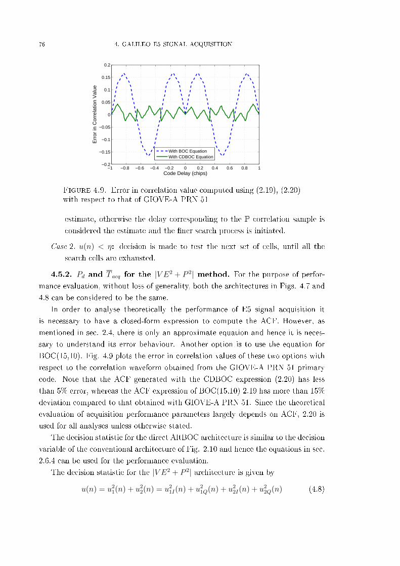
76 4. GALILEO E5 SIGNAL ACQUISITION
−1 −0.8 −0.6 −0.4 −0.2 0 0.2 0.4 0.6 0.8 1−0.2
−0.15
−0.1
−0.05
0
0.05
0.1
0.15
0.2
Code Delay (chips)
Err
or in
Cor
rela
tion
Val
ue
With BOC EquationWith CDBOC Equation
Figure 4.9. Error in correlation value computed using (2.19), (2.20)with respect to that of GIOVE-A PRN 51
estimate, otherwise the delay corresponding to the P correlation sample is
considered the estimate and the �ner search process is initiated.
Case 2. u(n) < η: decision is made to test the next set of cells, until all the
search cells are exhausted.
4.5.2. Pd and T acq for the |V E2 + P 2| method. For the purpose of perfor-mance evaluation, without loss of generality, both the architectures in Figs. 4.7 and
4.8 can be considered to be the same.
In order to analyse theoretically the performance of E5 signal acquisition it
is necessary to have a closed-form expression to compute the ACF. However, as
mentioned in sec. 2.4, there is only an approximate equation and hence it is neces-
sary to understand its error behaviour. Another option is to use the equation for
BOC(15,10). Fig. 4.9 plots the error in correlation values of these two options with
respect to the correlation waveform obtained from the GIOVE-A PRN 51 primary
code. Note that the ACF generated with the CDBOC expression (2.20) has less
than 5% error, whereas the ACF expression of BOC(15,10) 2.19 has more than 15%
deviation compared to that obtained with GIOVE-A PRN 51. Since the theoretical
evaluation of acquisition performance parameters largely depends on ACF, 2.20 is
used for all analyses unless otherwise stated.
The decision statistic for the direct AltBOC architecture is similar to the decision
variable of the conventional architecture of Fig. 2.10 and hence the equations in sec.
2.6.4 can be used for the performance evaluation.
The decision statistic for the |V E2 + P 2| architecture is given by
u(n) = u21(n) + u2
2(n) = u21I(n) + u2
1Q(n) + u22I(n) + u2
2Q(n) (4.8)

4.5.∣∣V E2 + P 2
∣∣ METHOD FOR ALTBOC 77
Again, assuming the Gaussian distribution and statistical independence of the
individual correlation outputs, one can compute the detection and false alarm prob-
abilities.
Under the hypothesis H0 when there is no signal present, the decision statistic
has a central chi-square distribution with four degrees of freedom (2.29).
Under the hypothesis H1 when the signal is present the decision statistic has a
non-central chi-square distribution with four degrees of freedom with PDF ps(x) and
non-centrality parameter λ2 = m21I +m2
1Q +m22I +m2
2Q and Pd is given by (2.30).
In both the Direct AltBOC and the |V E2 + P 2| methods, one can perform a
non-coherent integration of the decision statistic to improve the sensitivity, and
correspondingly the degree of freedom parameter of the chi-square distributions will
have to be multiplied by the number of non-coherent summations. Therefore if
Nnc is the number of non-coherent summations, then the decision statistic in the
|V E2 + P 2| method will have 4Nnc degrees of freedom.
In these analyses and simulations a Pfa = 10−3 was considered and a pre-
detection coherent integration time of one millisecond was assumed. Note that,
in practice, the penalty due to false alarm will be comparatively less in the case of
the |V E2 + P 2| method, as one will be entering the �ner code delay search process
and not the tracking process. For the approaches with a two-step search process,
only the coarse (initial) step is considered since it is the dominant part.
Fig. 4.10 shows the worst case probability of detection for BPSK and AltBOC.
To show the step size required to achieve BPSK-like correlation losses and to show
the e�ect of larger step size, δt= 0.083 as well as δt=0.5 are chosen for AltBOC. Note
that a loss of 6.3 dB between AltBOC with δt=0.5 and BPSK δt=0.5 (or AltBOC
=0.083) can be noted from the plot.
Fig. 4.11 shows the average probability of detection for BPSK and AltBOC with
δt as in Fig. 4.10. The average correlation loss scenario stems from the fact that one
will not always encounter the worst case and RCPO will have a uniform distribution
in [0, δt). Note that the di�erence between AltBOC δt=0.5 and the BPSK δt=0.5
reduces to around 2.2 dB in such a case.
Fig. 4.12 shows the average probability of detection for the acquisition ap-
proaches considered in Fig. 4.2. Note that the di�erence in the power distribution
among di�erent approaches is evident with the probability of detection curve.
Figs. 4.13 and 4.14 provide the theoretical and simulated average and worst
case probability of detection for the |V E2 + P 2| method with both δt=0.5 and 0.85
scenarios respectively.
In Fig. 4.13 one can see that the average probability of detection for the
|V E2 + P 2| method is 0.4 dB worse than the BPSK case, and that the |V E2 + P 2|method outperforms Direct AltBOC approach by about 2.2 dB. Fig. 4.14 shows

78 4. GALILEO E5 SIGNAL ACQUISITION
20 25 30 35 40 45 500
0.1
0.2
0.3
0.4
0.5
0.6
0.7
0.8
0.9
1
Carrier to Noise Ratio C/N0 (dBHz)
Pro
babi
lity
of D
etec
tion
Pd
Best CaseBPSK Delta=0.5AltBOC Delta=0.083AltBOC Delta=0.5
Figure 4.10. Worst case probability of detection for BPSK and AltBOC
20 25 30 35 40 45 500
0.1
0.2
0.3
0.4
0.5
0.6
0.7
0.8
0.9
1
Carrier to Noise Ratio C/N0 (dBHz)
Pro
babi
lity
of D
etec
tion
Pd
Best CaseBPSK Delta=0.5AltBOC Delta=0.083AltBOC Delta=0.5
Figure 4.11. Average probability of detection for BPSK and AltBOC

4.5.∣∣V E2 + P 2
∣∣ METHOD FOR ALTBOC 79
20 25 30 35 40 45 500
0.1
0.2
0.3
0.4
0.5
0.6
0.7
0.8
0.9
1
Carrier to Noise Density C/N0 (dBHz)
Pro
babi
lity
of D
etec
tion
Pd
Best CaseE5aQ−SSBE5a−SSBE5a & E5b – DSBE5aQ−FICE5 Pilots – FICE5 Pilots & Data FICDirect AltBOC
Figure 4.12. Average Pd for di�erent acquisition approaches
20 25 30 35 40 45 500
0.1
0.2
0.3
0.4
0.5
0.6
0.7
0.8
0.9
1
Carrier to Noise Density C/N0 (dBHz)
Pro
babi
lity
of D
etec
tion
Pd
BPSK theor.AltBOC δ
t=0.5 theor.
VEP δt=0.5 theor.
VEP δt=0.85 theor.
BPSK sim.AltBOC δ
t=0.5 sim.
VEP δt=0.5 sim.
VEP δt=0.85 sim.
Figure 4.13. Average Pd for AltBOC and |V E2 + P 2| methods (�:theory, •: simulation)
that the worst case loss for the |V E2 + P 2| method is only 1 dB worse than that of
the BPSK method, and there is an improvement of 5.3 dB compared to the Direct
AltBOC approach.
Figures. 4.15 and 4.16 compare the mean acquisition time for the probability of
detection scenarios considered in Fig. 4.13 and 4.145. Observe that the |V E2 + P 2|method for the average case with δt=0.85 chip step performs better than the BPSK
case with δt=0.5. This is also true for the worst case scenario, but only at higher
5Since Pd in�uences T acq and Pd is less than 0.1 for C/N0 values below 30 dBHz, the Monte-Carlo
simulations do not yield proper results. Hence, T acq for C/N0 values below 30 dBHz are plotted.
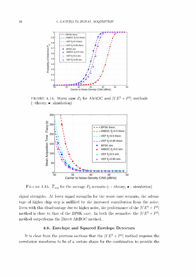
80 4. GALILEO E5 SIGNAL ACQUISITION
20 25 30 35 40 45 500
0.1
0.2
0.3
0.4
0.5
0.6
0.7
0.8
0.9
1
Carrier to Noise Density C/N0 (dBHz)
Pro
babi
lity
of D
etec
tion
Pd
BPSK theor.AltBOC δ
t=0.5 theor.
VEP δt=0.5 theor.
VEP δt=0.85 theor.
BPSK sim.AltBOC δ
t=0.5 sim.
VEP δt=0.5 sim.
VEP δt=0.85 sim.
Figure 4.14. Worst case Pd for AltBOC and |V E2 + P 2| methods(�:theory, •: simulation)
30 35 40 45 500
50
100
150
200
250
300
Carrier to Noise Density C/N0 (dBHz)
Mea
n A
cqui
sitio
n T
ime
/Tac
q (s
)
BPSK theor.AltBOC δ
t=0.5 theor.
VEP δt=0.5 theor.
VEP δt=0.85 theor.
BPSK sim.AltBOC δ
t=0.5 sim.
VEP δt=0.5 sim.
VEP δt=0.85 sim.
Figure 4.15. T acq for the average Pd scenario (- - :theory, • : simulation)
signal strengths. At lower signal strengths for the worst case scenario, the advan-
tage of higher chip step is nulli�ed by the increased contribution from the noise.
Even with this disadvantage due to higher noise, the performance of the |V E2 + P 2|method is close to that of the BPSK case. In both the scenarios, the |V E2 + P 2|method outperforms the Direct AltBOC method.
4.6. Envelope and Squared Envelope Detectors
It is clear from the previous sections that the |V E2 + P 2| method requires the
correlation waveforms to be of a certain shape for the combination to provide the

4.6. ENVELOPE AND SQUARED ENVELOPE DETECTORS 81
30 32 34 36 38 40 42 44 46 48 500
50
100
150
200
250
300
Carrier to Noise Density C/N0 (dBHz)
Mea
n A
cqui
sitio
n T
ime
/Tac
q (s
)
BPSK theor.AltBOC δ
t=0.5 theor.
VEP δt=0.5 theor.
VEP δt=0.85 theor.
BPSK sim.AltBOC δ
t=0.5 sim.
VEP δt=0.5 sim.
VEP δt=0.85 sim.
Figure 4.16. T acq for the worst case Pd scenario (- - :theory, • :simulation)
expected result. However, the shape of the correlation function depends on the front-
end �lter used in the receiver. In addition, the combination could be either of the
�squared envelope� or �envelope� type. This section considers these two parameters
to analyse their e�ect on the |V E2 + P 2|method. In a general sense, the |V E2 + P 2|method can be considered as a �Delayed Addition� (DA) method, and this is the
generic term used in this section.
4.6.1. The DA method and the e�ect of pre-correlation �ltering. It
was shown in the previous section that the nulls in the AltBOC correlation wave-
form severely a�ect acquisition, and this can be mitigated by using the |V E2 + P 2|method, a special case of the DA method.
Let Ik1 , Qk1 be the correlation values corresponding to the local code C(t − τ)
and Ik2 , Qk2 be the correlation values corresponding to the local code C(t− τ−DTc).The parameter D ∈ (0, 1] is chosen to obtain the BPSK-like correlation triangle. In
the DA-squared envelope method, the decision statistic is formulated as:
da_zs =Nnc∑k=1
sk, sk = I2k1
+Q2k1
+ I2k2
+Q2k2
(4.9)
Now, observe the shape of the correlation waveform by combining the envelope
outputs in the DA method instead of squared envelope outputs. To do this, let the
DA-envelope decision statistic be formulated as:
da_ze =Nnc∑k=1
ek, ek =√I2k1
+Q2k1
+√I2k2
+Q2k2
(4.10)

82 4. GALILEO E5 SIGNAL ACQUISITION
−2 −1.5 −1 −0.5 0 0.5 1 1.5 20
0.2
0.4
0.6
0.8
1
1.2
1.4
Code Delay (chips)
Nor
mal
ized
Abs
olut
e C
orre
latio
n V
alue
Direct AltBOCDA−Sq.EnvelopeDA−Envelope
Figure 4.17. Correlation waveforms, in�nite bandwidth
For both the methods D=0.167 chip is used, which gives a BPSK-like triangle. Figs.
4.17 and 4.18 show the correlation waveform and the e�ect of code search step,
without pre-correlation �ltering. Figs. 4.19 and 4.20 have a 5th order Butterworth
�lter with a 3 dB bandwidth of 50 MHz. The outputs are normalised with respect
to the Direct AltBOC case. Observe that the correlation output in the DA-envelope
case (with �ltering) is slightly better than that of the DA-squared envelope case and
has smaller triangles sitting on top of it. In addition, the �at region from about 0.5
to 0.85 chip search steps in the case of the DA-squared envelope is extended to about
1.0 chip in the case of the DA-envelope method. In addition, the �ltering alters the
position of the sub-peaks. For example the second sub-peak is moved close to 0.3
chips from the initial 0.33 of the in�nite bandwidth case. The implication of these
di�erences on the acquisition performances are analysed in the following section.
4.6.2. The DA-envelope detector architecture. The correlator architec-
ture for the DA-envelope method can be realised in two ways. In the �rst approach
the output of the correlators separated in time by DTc can be added together to
obtain the in-phase and quadrature phase correlator outputs. The parameter D
then depends on the sampling frequency. Figure 4.21 illustrates this architecture.
On the other hand, if the second set of in-phase and quadrature phase correlation
values can be generated in a similar way to Fig. 4.8 with a separate set of local code
replicas, then D can be controlled by appropriately programming the phase of the
NCO that is used to generate the code.

4.6. ENVELOPE AND SQUARED ENVELOPE DETECTORS 83
0 0.5 1 1.5 20
0.5
1
1.5
Code Search Step Size (chips)
Nor
mal
ized
Cor
rela
tion
Loss
Direct AltBOCDA−Sq.EnvelopeDA−Envelope
Figure 4.18. Correlation loss, in�nite bandwidth
−2 −1 0 1 20
0.2
0.4
0.6
0.8
1
1.2
1.4
Code Delay (chips)
Nor
mal
ized
Abs
olut
e C
orre
latio
n V
alue
Direct AltBOCDA−Sq.EnvelopeDA−Envelope
Figure 4.19. Correlation waveforms, 50MHz bandwidth

84 4. GALILEO E5 SIGNAL ACQUISITION
0 0.5 1 1.5 20
0.5
1
1.5
Code Search Step Size (chips)
Nor
mal
ized
Cor
rela
tion
Loss
Direct AltBOCDA−Sq.EnvelopeDA−Envelope
Figure 4.20. Correlation loss, 50MHz bandwidth
cDT
cDT
Code
Generator
Complex
Carrier
2
2
)()(
Envelope
t Tt c
_da ze
2
2
( )IFr t
t Tt c
Figure 4.21. Detector architecture, DA-envelope method

4.7. EXPLOITING SECONDARY CODES TO INCREASE ACQ. PERFORMANCE 85
4.6.3. Performance analysis. As explained earlier, the acquisition perfor-
mance of the DA-squared envelope is straightforward to calculate, but for the DA-
envelope method it is not.
The closed form approximations of the in�nite series expressions derived in Hu
and Beaulieu (2005b,a) can be used in this context. Note that for the DA-squared
envelope method there are 4Nnc degrees of freedom because each decision statistic
comprises two sets of correlator outputs. Coherent integration duration Tcoh of
one millisecond is used with probability of false alarm Pfa set to 10−3. For the
DA methods a chip search step of 0.85 is used. As a reference, the probability of
detection curve for the Direct AltBOC acquisition is also considered. Fig. 4.22 shows
the probability of detection curves for Nnc=1, Nnc=4 and Nnc=8. Observe that the
DA methods perform better for higher signal strengths at smaller values of Nnc. As
the signal strength decreases or as Nnc increases, the Direct AltBOC behaves well.
This can be explained as follows. When Nnc=1, the decision statistic will have two
signal components and two noise components. At high SNR values, the e�ect of
an increase in noise is masked. At low SNR the increase in noise because of the
two noise components reduces the advantage of the DA method. As Nnc increases,
the Direct AltBOC method will experience more SNR gain compared to the DA
methods, again because of the additional noise components in the DA method.
At smaller values of SNR the DA-envelope method provides about 1 dB improve-
ment over the DA-squared envelope method. A small part of this improvement is
due to the envelope detector itself (as discussed earlier) and the rest is due to the
reduced loss in the correlation output in the case of the DA-envelope method com-
pared to the DA-squared Envelope method. As Nnc increases the advantage of
the DA-envelope method reduces because both the decision statistics tend towards
Gaussian distributions according to the central limit theorem.
Fig. 4.23 shows the probability of detection curves for the DA-squared envelope
method and the DA-envelope method at code search steps of 0.85 and 1.0 respec-
tively. Note that both the methods behave similarly as expected from the correlation
waveform. Fig. 4.24 compares the T acq for the two methods. Here the search step
used for the DA-squared envelope method is 0.85 and the search step used for DA-
envelope method is 1.0 since both the methods have similar probability of detection
performances. The Direct AltBOC method is also shown for reference. Note that an
improvement of about 10% is obtained with the DA-envelope method with respect
to the DA-squared envelope method.
4.7. Exploiting Secondary Codes to Increase Acquisition Performance
The architecture presented in this section takes a di�erent approach to perform
longer integrations to that of non-coherently combining one primary code period

86 4. GALILEO E5 SIGNAL ACQUISITION
20 25 30 35 40 45 500
0.1
0.2
0.3
0.4
0.5
0.6
0.7
0.8
0.9
1
C/N0 (dBHz) at the detector input
Pro
babi
lity
of D
etec
tion
Pd
Direct AltBOCDA−Sq.EnvelopeDA−Envelope
20 25 30 35 40 45 500
0.1
0.2
0.3
0.4
0.5
0.6
0.7
0.8
0.9
1
C/N0 (dBHz) at the detector input
Pro
babi
lity
of D
etec
tion
Pd
Direct AltBOCDA−Sq.EnvelopeDA−Envelope
20 25 30 35 40 45 500
0.1
0.2
0.3
0.4
0.5
0.6
0.7
0.8
0.9
1
C/N0 (dBHz) at the detector input
Pro
babi
lity
of D
etec
tion
Pd
Direct AltBOCDA−Sq.EnvelopeDA−Envelope
Figure 4.22. Probability of detection, Nnc=1 (top), Nnc=4 (Mid-dle), Nnc=8 (bottom)

4.7. EXPLOITING SECONDARY CODES TO INCREASE ACQ. PERFORMANCE 87
20 25 30 35 40 45 500
0.1
0.2
0.3
0.4
0.5
0.6
0.7
0.8
0.9
1
C/N0 (dBHz) at the detector input
Pro
babi
lity
of D
etec
tion
Pd
DA−EnvelopeDA−Sq.Envelope
Figure 4.23. Pd for δt=0.85 (DA-squared envelope) and δt=1.0 (DA-envelope); Nnc=1
20 25 30 35 40 45 5010
1
102
103
104
105
106
C/N0 (dBHz) at the detector input
Mea
n A
cqui
sitio
n T
ime
/Tac
q (s
)
Direct AltBOCDA−Sq.EnvelopeDA−Envelope
Figure 4.24. T acq comparison; Nnc=1
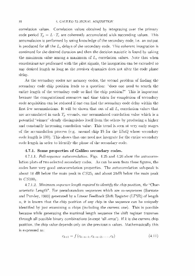
88 4. GALILEO E5 SIGNAL ACQUISITION
correlation values. Correlation values obtained by integrating over the primary
code period Tp = L · Tc are coherently accumulated with succeeding values. This
accumulation is performed by using knowledge of the secondary code, i.e. an output
is produced for all the Ls delays of the secondary code. This coherent integration is
continued for the desired duration and then the decision statistic is found by taking
the maximum value among a maximum of Ls correlation values. Note that when
correlations are performed with the pilot signals, the integration can be extended to
any desired length as long as the receiver dynamics does not alter the code phase
delay.
As the secondary codes are memory codes, the second problem of �nding the
secondary code chip position leads to a question: �does one need to search the
entire length of the secondary code to �nd the chip position?� This is important
because the computational resources and time taken for completion of secondary
code acquisition can be reduced if one can �nd the secondary code delay within the
�rst few accumulations. It will be shown that out of all Ls correlation values that
are accumulated in each Tp seconds, one accumulated correlation value which is a
potential �winner� clearly distinguishes itself from the others by producing a higher
and constantly increasing correlation value. This trend is seen at very early stages
of the accumulation process (e.g. around chip 15 for the E5aQ whose secondary
code length is 100). This shows that one need not integrate for the entire secondary
code length in order to identify the phase of the secondary code.
4.7.1. Some properties of Galileo secondary codes.
4.7.1.1. Full-sequence autocorrelation. Figs. 4.25 and 4.26 show the autocorre-
lation plots of two selected secondary codes. As can be seen from these �gures, the
codes have very good autocorrelation properties. The autocorrelation sub-peak is
about 18 dB below the main peak in CS251 and about 21dB below the main peak
in CS1001.
4.7.1.2. Minimum sequence length required to identify the chip position, the �Char-
acteristic Length�. For pseudorandom sequences which are m-sequences (Sarwate
and Pursley, 1980) generated by a Linear Feedback Shift Register (LFSR) of length
n, it is known that the chip position of any chip in the sequence can be uniquely
identi�ed by just examining n chips (including the current one). This is possible
because while generating the maximal length sequence the shift register traverses
through all possible binary combinations (except `all zeros'). If k is the current chip
position, the chip value depends only on the previous n values. Mathematically this
is expressed as:
ck+1 = f (ck−n−1, ck−n−2, . . . , ck) (4.11)

4.7. EXPLOITING SECONDARY CODES TO INCREASE ACQ. PERFORMANCE 89
−10 −5 0 5 10−30
−25
−20
−15
−10
−5
0
Chip Shift (Chips)
Nor
mal
ized
Cor
rela
tion
Val
ue (
dB)
Figure 4.25. Autocorrelation plot of the secondary code CS251
−40 −20 0 20 40−40
−30
−20
−10
0
Chip Shift (Chips)
Nor
mal
ized
Cor
rela
tion
Val
ue (
dB)
Figure 4.26. Autocorrelation plot of the secondary code CS1001

90 4. GALILEO E5 SIGNAL ACQUISITION
The length which is just su�cient to identify the chip shift is called the linear span
(LS) L of that code sequence(Cherubini and Benvenuto, 2002; Chan and Games,
1990). Note that the Berlekamp-Massey algorithm (Cherubini and Benvenuto, 2002)
can be used to reconstruct the entire sequence if one considers 2L chips (without the
knowledge of feedback taps). However, because the memory codes are not directly
generated using LFSR, use is made of the general concept of LS and not the sequence
reconstruction.
For the Gold codes (as in the case of those used in GPS L1 C/A) generated with
two n-bit shift registers, the LS is 2n chips. This implies that if the sequence is
broken into smaller sequences, each of length equal to the LS, then no two of these
smaller sequence bit patterns will be identical to each other.
This concept can be extended to the memory codes. Even though the memory
codes are not generated using a LFSR, their spans can be used. This span can be
referred to as the characteristic length (CL) (and use the same notation L) of thesequence.
4.7.1.3. Procedure for evaluating the characteristic length. In order to do this,
the following these steps are used:
(1) Let k be the number of contiguous `zeros' or `ones' (whichever is maximum)
in the sequence whose length is Ls.
(2) Form a matrixM with the partial sequences of length k as the rows where
each row is shifted by one bit with respect to the previous row. Hence the
size of the matrix will be Ls · k.
M =
c1 c2 . . ck
c2 c3 . . ck+1
. . . . .
. . . . .
cNs−k cNs−k−1 . . cNs. . . . .
cNs c1 . . ck−1
(4.12)
(3) Examine the matrix for identical rows. If any two rows are identical then
increment k and repeat Step 2 until no two rows of the matrix are iden-
tical. The uniqueness of the rows can be found by computing the linear
rank correlation coe�cient matrix X = CORR(M) of the rows of M and
examining whether any entry of X is unity.
(4) The smallest value of k which satis�es the condition in Step 3 is the CL Lof the sequence.
The CL obtained using the aforementioned procedure for di�erent secondary code
sequences of Galileo is given in Table 4.3. For the E5 secondary code, which is
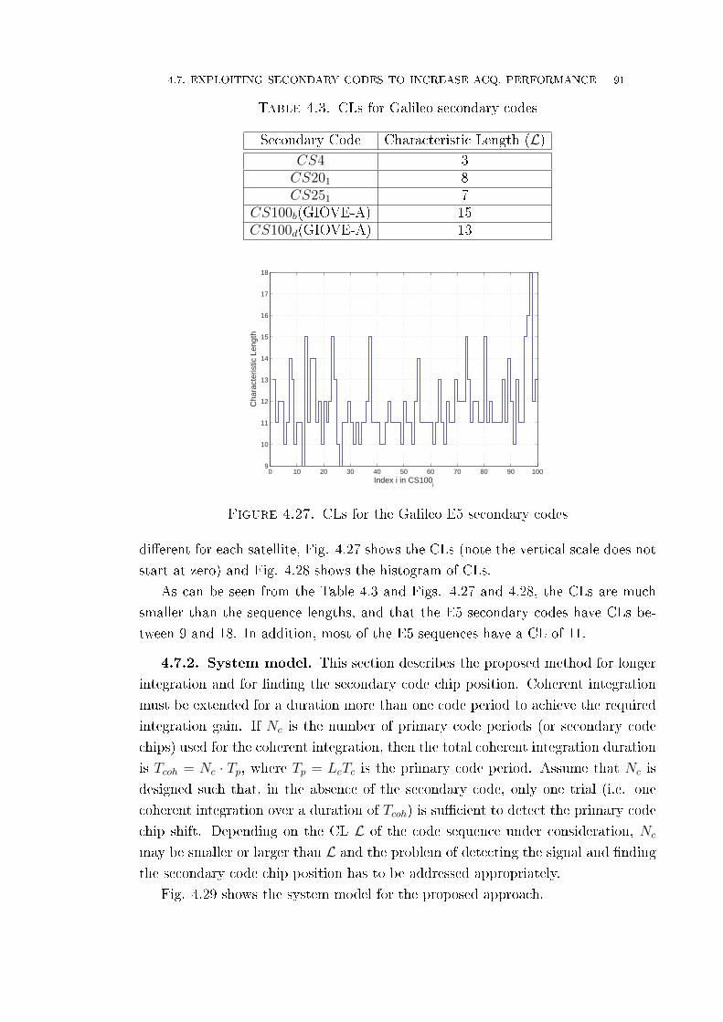
4.7. EXPLOITING SECONDARY CODES TO INCREASE ACQ. PERFORMANCE 91
Table 4.3. CLs for Galileo secondary codes
Secondary Code Characteristic Length (L)CS4 3CS201 8CS251 7
CS100b(GIOVE-A) 15CS100d(GIOVE-A) 13
0 10 20 30 40 50 60 70 80 90 1009
10
11
12
13
14
15
16
17
18
Index i in CS100i
Cha
ract
eris
tic L
engt
h
Figure 4.27. CLs for the Galileo E5 secondary codes
di�erent for each satellite, Fig. 4.27 shows the CLs (note the vertical scale does not
start at zero) and Fig. 4.28 shows the histogram of CLs.
As can be seen from the Table 4.3 and Figs. 4.27 and 4.28, the CLs are much
smaller than the sequence lengths, and that the E5 secondary codes have CLs be-
tween 9 and 18. In addition, most of the E5 sequences have a CL of 11.
4.7.2. System model. This section describes the proposed method for longer
integration and for �nding the secondary code chip position. Coherent integration
must be extended for a duration more than one code period to achieve the required
integration gain. If Nc is the number of primary code periods (or secondary code
chips) used for the coherent integration, then the total coherent integration duration
is Tcoh = Nc · Tp, where Tp = LcTc is the primary code period. Assume that Nc is
designed such that, in the absence of the secondary code, only one trial (i.e. one
coherent integration over a duration of Tcoh) is su�cient to detect the primary code
chip shift. Depending on the CL L of the code sequence under consideration, Nc
may be smaller or larger than L and the problem of detecting the signal and �nding
the secondary code chip position has to be addressed appropriately.
Fig. 4.29 shows the system model for the proposed approach.
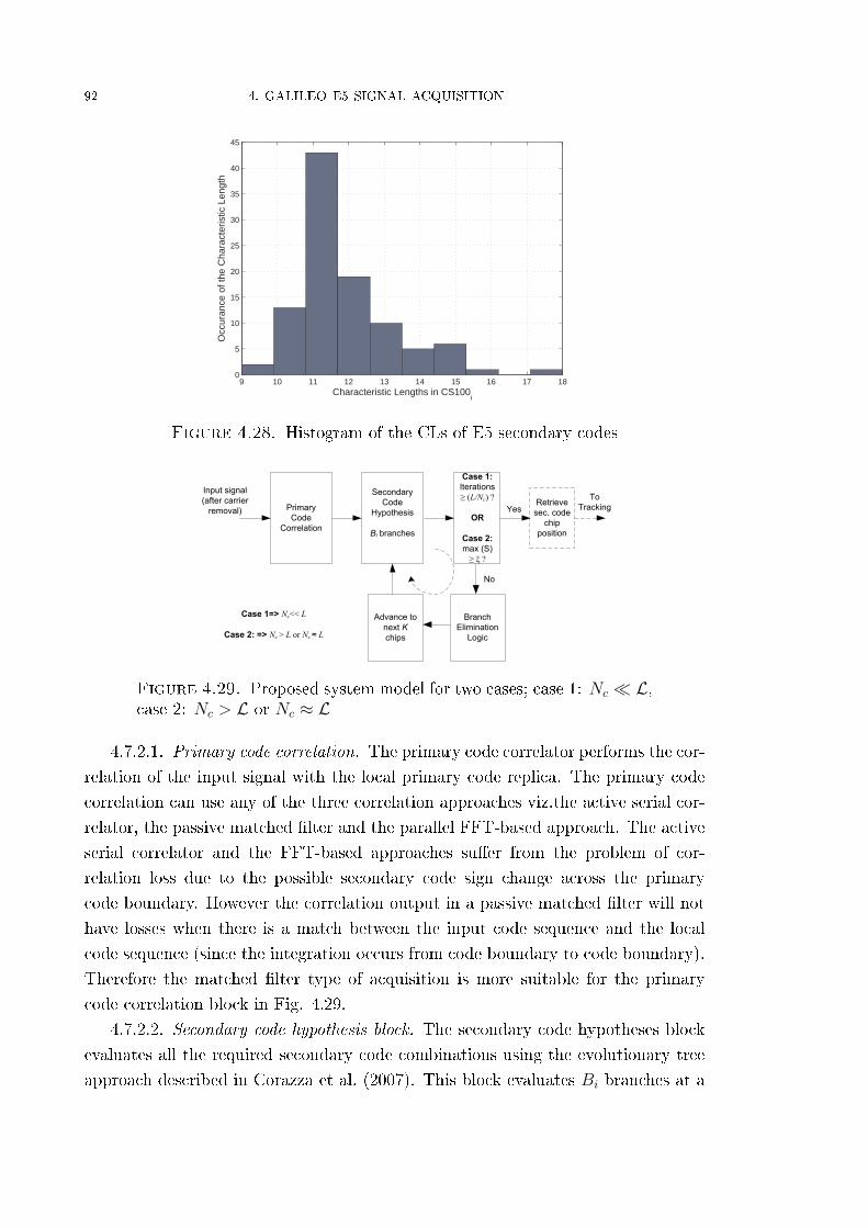
92 4. GALILEO E5 SIGNAL ACQUISITION
9 10 11 12 13 14 15 16 17 180
5
10
15
20
25
30
35
40
45
Characteristic Lengths in CS100i
Occ
uran
ce o
f the
Cha
ract
eris
tic L
engt
h
Figure 4.28. Histogram of the CLs of E5 secondary codes
Primary
Code
Correlation
Secondary
Code
Hypothesis
Bi branches
Branch
Elimination
Logic
Case 1:
Iterations
≥ (L/Nc) ?
OR
Case 2:
max (S)
≥ ξ ?
Advance to
next K
chips
No
Yes
Input signal
(after carrier
removal)Retrieve
sec. code
chip
position
To
Tracking
Case 1=> Nc<< L
Case 2: => Nc > L or Nc ≈ L
Figure 4.29. Proposed system model for two cases; case 1: Nc � L,case 2: Nc > L or Nc ≈ L
4.7.2.1. Primary code correlation. The primary code correlator performs the cor-
relation of the input signal with the local primary code replica. The primary code
correlation can use any of the three correlation approaches viz.the active serial cor-
relator, the passive matched �lter and the parallel FFT-based approach. The active
serial correlator and the FFT-based approaches su�er from the problem of cor-
relation loss due to the possible secondary code sign change across the primary
code boundary. However the correlation output in a passive matched �lter will not
have losses when there is a match between the input code sequence and the local
code sequence (since the integration occurs from code boundary to code boundary).
Therefore the matched �lter type of acquisition is more suitable for the primary
code correlation block in Fig. 4.29.
4.7.2.2. Secondary code hypothesis block. The secondary code hypotheses block
evaluates all the required secondary code combinations using the evolutionary tree
approach described in Corazza et al. (2007). This block evaluates Bi branches at a

4.7. EXPLOITING SECONDARY CODES TO INCREASE ACQ. PERFORMANCE 93
time.
Case 1. If Nc � L, the value of B will be 2Nc−1 to start with. Hence
Bi =
2Nc−1 i = 0
Bi−1 − Ei i 6= 0(4.13)
where Ei is the number of branches eliminated in the ith iteration.
Case 2. If Nc > L or Nc ≈ L, then the value of B at each iteration will depend
on the strength of the received signal. This means that as one extends
the integration time, the branch elimination logic can better decide on the
branches to be eliminated.
4.7.2.3. Branch elimination logic. The branch elimination logic examines all the
hypotheses output by the secondary code hypothesis block. The criterion for any
branch elimination is the lower correlation value relative to other branches. Let
S = (s1, s2, . . . , sBi)Tbe the vector containing the entire secondary code hypotheses,
where si is the ith secondary code hypothesis. A vector D containing the di�erence
of S with respect to the maximum is formed. Thus:
D = max(S)− S (4.14)
At each iteration, Ei number of branches whose correlation value exceeds a prede-
�ned threshold ξ are eliminated.
4.7.2.4. Decision to end the iteration.
Case 1. When Nc � L (which is the case when the signal strength is moderately
high) one would have detected the primary code (and its chip shift) before
determining the secondary code chip position. In this case the iteration
should be continued to determine the secondary code chip position and hence
the emphasis is on the crossing point of the CL. Thus the iteration ends when
the total number of primary code periods used in all the iterations is greater
than L. At each stage, the secondary code is advanced by K chips (typically
K = Nc).
Case 2. When Nc > L or Nc ≈ L, (which is the case when the signal strength is
low) one needs to integrate long enough so that the decision statistic
Λ = max (λ(si)) i = [0, Bi − 1] (4.15)
is greater than the threshold ξ, to detect the primary code. Here λ(si) is
the detector output of the ith secondary code hypothesis. Hence in this
case the emphasis is on the signal (i.e. primary code) detection and the
hypothesis which causes the decision statistic to cross the threshold is used

94 4. GALILEO E5 SIGNAL ACQUISITION
5 10 15 200
1
2
3
4x 10
6
Number of primary code periods
Max
imum
cor
rela
tion
valu
e
Figure 4.30. Correlation value trend for increasing number of pri-mary code period integrations (di�erent colours show all the 100 hy-potheses)
to determine the secondary code chip position. At each stage, the secondary
code is advanced by K chips, which is su�cient to eliminate some of the
branches.
4.7.2.5. Secondary code chip position retrieval. The secondary code hypothesis
that wins corresponds to a sub-sequence within the complete secondary code. The
process of obtaining this sub-sequence is equivalent to the �traceback� technique used
in Viterbi decoding(Viterbi and Omura, 1979). Thus retrieving the chip position is
performed by searching for this sub-sequence in the larger sequence and determining
the index of the shift.
4.7.3. Results. In order to evaluate the performance of the proposed method,
150ms of real data collected from Septentrio GeNeRX1 receiver for the E5 signal
from the GIOVE-A satellite was used. Determining the secondary code chip position
is di�cult in the case of E5 since the primary code period is only one millisecond
and the secondary code 100 chips for the pilot signals.
The procedure followed to acquire the E5 signal is:
(1) acquire E5aQ pilot signal whilst �nding the secondary code chip position,
and then
(2) use this information of the secondary code chip position and acquire E5
signal.
Fig. 4.30 shows the trend in correlation values for increasing integration time. To
show the applicability of the proposed method all 100 hypotheses were used. Note
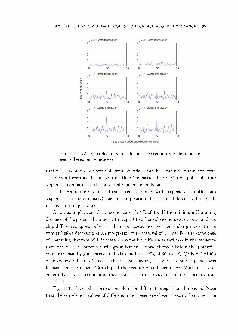
4.7. EXPLOITING SECONDARY CODES TO INCREASE ACQ. PERFORMANCE 95
0 50 1000
1
2
3
4x 10
6 2ms Integration
0 50 1000
1
2
3
4x 10
6 4ms Integration
0 50 1000
1
2
3
4x 10
6 8ms Integration
0 50 1000
1
2
3
4x 10
6 12ms Integration
0 50 1000
1
2
3
4x 10
6 16ms Integration
0 50 1000
1
2
3
4x 10
6
Secondary code sub−sequence index
Cor
rela
tion
valu
e
20ms Integration
Figure 4.31. Correlation values for all the secondary code hypothe-ses (sub-sequence indices)
that there is only one potential �winner�, which can be clearly distinguished from
other hypotheses as the integration time increases. The deviation point of other
sequences compared to the potential winner depends on:
i. the Hamming distance of the potential winner with respect to the other sub
sequences (in the X matrix), and ii. the position of the chip di�erences that result
in this Hamming distance.
As an example, consider a sequence with CL of 15. If the minimum Hamming
distance of the potential winner with respect to other sub-sequences is 4 (say) and the
chip di�erences appear after 11, then the closest incorrect contender grows with the
winner before deviating at an integration time interval of 11 ms. For the same case
of Hamming distance of 4, if there are some bit di�erences early on in the sequence
then the closest contender will grow but in a parallel track below the potential
winner eventually guaranteed to deviate at 11ms. Fig. 4.30 used GIOVE-A CS100b
code (whose CL is 15) and in the received signal, the winning sub-sequence was
located starting at the 46th chip of the secondary code sequence. Without loss of
generality, it can be concluded that in all cases this deviation point will occur ahead
of the CL.
Fig. 4.31 shows the correlation plots for di�erent integration durations. Note
that the correlation values of di�erent hypotheses are close to each other when the

96 4. GALILEO E5 SIGNAL ACQUISITION
0 1 2 3 4 5
x 104
0
0.5
1
1.5
2
2.5
3
3.5
4x 10
5
Sample number
Cor
rela
tion
valu
e
3.268 3.27 3.272 3.274 3.276 3.278 3.28
x 104
0
0.5
1
1.5
2
2.5
3
3.5
4x 10
5
Sample number
Cor
rela
tion
valu
e
Figure 4.32. Absolute correlation value of the E5 signal (right pic-ture is the zoomed version around the peak);1 ms integration
0 2 4 6 8 10
x 104
0
5
10
15x 10
5
Sample number
Cor
rela
tion
valu
e
3.268 3.27 3.272 3.274 3.276 3.278 3.28
x 104
0
5
10
15x 10
5
Sample number
Cor
rela
tion
valu
e
Figure 4.33. Absolute correlation value of the E5 signal (right pic-ture is the zoom version around the peak); 4ms integration using thesecondary code chip position detection algorithm; data collected forGIOVE-A satellite on 5th Feb 2008
integration time is less than the CL (because the primary code period is 1 millisecond
for E5, the terms `integration time' and `number of primary code periods can be used
interchangeably). As soon as the integration time reaches the CL, a clear peak pops
up.
The secondary code chip position obtained in this case was 46 which corresponds
to the sub-sequence [1 0 0 0 1 0 1 1 0 0 0 1 1 1 0]. Using this information the E5
signal was acquired with 1 millisecond and 4 millisecond integrations. The plots
(and the zoomed versions around the peak) are shown in Figs. 4.32 and 4.33.
4.8. Summary
The �rst part of this chapter discussed the complexity and problems with the
Galileo E5 signal acquisition and revisited di�erent strategies which address these
problems. The probability of detection and the mean acquisition time for these
strategies were studied, especially concentrating on the |V E2 + P 2| method along
with the acquisition engine architecture. For the same probability of detection,
compared to the Direct AltBOC approach, the |V E2 + P 2| method results in an

4.8. SUMMARY 97
improvement in C/N0 of about 2.2 dB for the average scenario and about 5.3 dB
for the worst case scenario. In addition an interesting observation shows that the
correlation loss in the |V E2 + P 2| method remains constant for chip step sizes from
0.5 to 0.85 which can be exploited to reduce the mean acquisition time by 41%. It
was concluded that the |V E2 + P 2| method with this step size, is a good candidate
for implementation in Galileo E5 receivers.
Next, the performance of squared-envelope and envelope detectors applied to
the |V E2 + P 2| method, which is a speci�c case of the DA method were analysed.
It was shown that for a �xed code search step size of 0.6 chips, the DA-envelope
method improves the probability of detection by about 1dB. For a �xed probability
of detection, the code search step in the case of the DA-envelope method can be
increased, thus reducing the mean acquisition time by about 10% compared to the
DA-squared envelope method.
The problem of coherent integration over periods longer than one primary code
length and the acquisition of secondary code chip position was also examined. An
acquisition engine architecture which can handle both these problems simultaneously
was proposed. The acquisition architecture presented in this chapter is unique in the
sense of achieving longer integration by exerting secondary codes, and also acquiring
the secondary code chip position as a by-product of the acquisition process. It was
shown that the secondary code chip shift can be uniquely identi�ed by shorter length
sequences than the code itself. Most of the E5 secondary codes of length 100 can be
identi�ed by shorter sequences of length of around 15.


CHAPTER 5
Galileo E5 Signal Tracking
5.1. Introduction
Due to their structure, Galileo E5 signals o�er a number of ways to synchronise
the signal and to demodulate the data. The presence of several parameters in the
AltBOC modulation from its four primary codes, four secondary codes, four phases
of a complex sub-carrier and two data components, all of which are appropriately
mapped onto four signal components, makes the e�cient synchronisation of the
AltBOC signal an interesting and challenging task. Several strategies for signal
acquisition have been discussed in sec. 4.2. A sequential search method to identify
the phase of the secondary code has been discussed in sec. 4.7. The subsequent step
of tracking the signal is the topic of this chapter.
This chapter describes the architectures required, and discusses the pros and cons
of several methods, for tracking the E5 signal. Sections 5.2 to 5.5 contain the work
published in ENC GNSS 2009 (Shivaramaiah et al., 2009a) and sec. 5.6 contains the
work published in IEEE VTC FALL 2009 (Shivaramaiah and Dempster, 2009a).
The contributions of this chapter are:
• Development of a generic tracking architecture for the Galileo E5 AltBOC
signal and deriving an equation for the code tracking error
• Proposal of a hybrid tracking architecture with pre-correlation combinationmethod to address the issue of coherent integration beyond one data bit
duration
• Proposal of an extended tracking range DLL that combines the bene�ts
of the wide tracking range DLL discriminator characteristics of the E5a
/ E5b signal and the more accurate DLL discriminator characteristics of
AltBOC(15,10)
This chapter is organised as follows. In sec. 5.2, a generic tracking architecture that
can describe several ways of tracking a Galileo E5 signal, i.e. an architecture that
generalises the use of several local reference signals, is described and an equation
for the code tracking error is derived. This is followed by a list of candidate local
reference signals and a brief discussion of the advantages and disadvantages of using
di�erent reference signals in sec. 5.3. The issues with the combination of several
components of the E5 signal are discussed in sec. 5.4. In sec. 5.5, hybrid tracking
99

100 5. GALILEO E5 SIGNAL TRACKING
architectures that address the issues mentioned in sec. 5.4 are studied and a pre-
correlation combination architecture is proposed. Results of real satellite signal
tracking with the proposed hybrid architecture are provided in sec. 5.5. In sec.5.6 a
unique way of combining the Delay Locked-Loop (DLL) of an architecture employing
a reference signal that results in a BPSK-like correlation waveform and the DLL of
the Direct AltBOC signal tracking architecture is presented.
5.2. A Generalised Tracking Architecture
The received signal at an intermediate frequency (IF) in the case of Galileo E5
AltBOC can be represented as (considering any one satellite):1
rIF (t) =√
2P · < [s(t− τ) · exp (ωIF t+ ωdt+ θ)] + nW (t) (2.22)
where P is the received power, ωIF is the intermediate frequency, ωd is the Doppler
frequency, θ is the phase of the received signal, s(t − τ) is the complex baseband
signal with a time delay τ with respect to the transmitted signal, and nW (t) is
additive white Gaussian noise. The complex baseband signal can be represented as
s(t) = sc(t) + jss(t). Hence (2.22) can be written as:
rIF (t) =√
2P (sc(t− τ) · cos (ω0t+ θ)− ss(t− τ) · sin (ω0t+ θ)) + nW (t) (5.1)
where ω0 = ωIF + ωd.
The cosine and sine components are generated according to the AltBOC modula-
tion scheme described in sec. 2.3. The receiver front-end typically uses a bandwidth
of at least 51.15 MHz so as to pass the �rst two main lobes of the signal spectrum.
As with the processing methods for the acquisition explained in sec. 4.2, the sig-
nal tracking can also use similar techniques to track the complete E5 AltBOC or
any component of the signal. The �rst method in which the E5a and E5b signals
are translated from their centre frequencies to the baseband is the Single Sideband
(SSB) method or the Double Sideband (DSB) method when components from both
the sidebands are combined. While referring to either SSB or DSB method where
the local reference signal is generated free of sub-carriers, generally the term Side-
band Translation (SBT) method is used (Margaria and Dovis, 2008). The second
method is the Full-band Independent Correlation (FIC) in which the local signal is
generated for the required signal component mapped onto the appropriate phase of
the sub-carrier. The third method is the 8-PSK-like processing which allows only
the complete E5 signal correlation by the use of a look-up-table (LUT). With the
�rst two methods, several combinations of signal components are possible with the
combination variables being coherent and non-coherent, data and pilot, E5a and
E5b.1This equation is same as (2.22)

5.2. A GENERALISED TRACKING ARCHITECTURE 101
Reference
Baseband Signal
Generator
Complex
Carrier
( )IFr t
Code
Loop
Filter
Code
NCO
1,my1( )y t
2 ( )y t( )x t
( )y t
1
1( 1)
nT
n T
dt
1T
1T
2,my *
1ˆs t
*
2ˆs t
*
0ˆs t
Carrier
Loop
Filter
Carrier
discrimin
ator
Carrier
NCO
0 ( )y t
2
2( 1)
nT
n T
dt
0,ly
2T
1
1( 1)
nT
n T
dt
Code
discrimin
ator
Figure 5.1. Generalised architecture for the E5 signal tracking
Fig. 5.1 shows a generalised tracking architecture for the E5 signal. This ar-
chitecture holds good for all three methods of processing mentioned in the previous
paragraph. The received signal is multiplied with the locally generated carrier to
obtain the baseband signal. For the SBT method:
x(t) = xSBT (t) = exp(−j(ω0t+ θ ± ωsct
))(5.2)
where ωsc = 2πfsc is the sub-carrier angular frequency and the preceding sign de-
pends on whether one is interested in E5a (−) or E5b (+). For the FIC and 8-PSK
methods:
x(t) = xFIC(t) = x8−PSK(t) = exp(−j(ω0t+ θ
))(5.3)
Without loss of generality, the analogue representation of the signals at di�erent
points in the tracking loop up to the integrate and dump stage can be used. The
received signal is multiplied with the complex carrier generated at IF plus the esti-
mated Doppler (ω0 = ωIF + ωd ) and the estimated phase (θ ) to obtain y(t). The
reference baseband signal generator produces three signals s∗0(t − τ), s∗1(t − τ) and
s∗2(t− τ) where τ is the estimate of the code delay. The output of the carrier mixer
is then multiplied by the reference baseband signal to obtain the individual sample
correlations y0(t), y1(t) and y2(t) corresponding to s∗0(t− τ), s∗1(t− τ) and s∗2(t− τ)
respectively. The output obtained by multiplying with the di�erent versions of the
reference signal are integrated over a speci�ed duration T1 seconds to use in the
code tracking loop and T2 seconds to use in the carrier tracking. The carrier dis-
criminator uses the prompt reference signal (e.g. arctan). The two integration times
are given two di�erent notations to show that two loops can operate with di�erent
integration durations when required (which is more generic). The code tracking in
this architecture uses the delay-locked loop (DLL), whose inputs are the correlation
values of the received signal with at least two time-displaced versions of the local
reference signal. Note that more than three �taps� can also be used, although this
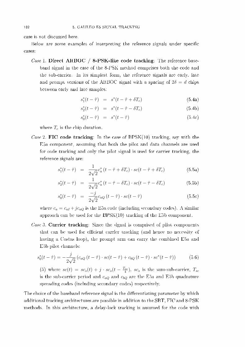
102 5. GALILEO E5 SIGNAL TRACKING
case is not discussed here.
Below are some examples of interpreting the reference signals under speci�c
cases:
Case 1. Direct AltBOC / 8-PSK-like code tracking: The reference base-
band signal in the case of the 8-PSK method comprises both the code and
the sub-carrier. In its simplest form, the reference signals are early, late
and prompt versions of the AltBOC signal with a spacing of 2δ = d chips
between early and late samples:
s∗1(t− τ) = s∗(t− τ + δTc) (5.4a)
s∗2(t− τ) = s∗(t− τ − δTc) (5.4b)
s∗0(t− τ) = s∗(t− τ) (5.4c)
where Tc is the chip duration.
Case 2. FIC code tracking: In the case of BPSK(10) tracking, say with the
E5a component, assuming that both the pilot and data channels are used
for code tracking and only the pilot signal is used for carrier tracking, the
reference signals are:
s∗1(t− τ) =1
2√
2c∗a (t− τ + δTc) · sc(t− τ + δTc) (5.5a)
s∗2(t− τ) =1
2√
2c∗a (t− τ − δTc) · sc(t− τ − δTc) (5.5b)
s∗0(t− τ) =−j
2√
2caQ (t− τ) · sc(t− τ) (5.5c)
where ca = caI +jcaQ is the E5a code (including secondary codes). A similar
approach can be used for the BPSK(10) tracking of the E5b component.
Case 3. Carrier tracking: Since the signal is comprised of pilot components
that can be used for e�cient carrier tracking (and hence no necessity of
having a Costas loop), the prompt arm can carry the combined E5a and
E5b pilot channels:
s∗0(t− τ) = − j
2√
2(caQ (t− τ) · sc(t− τ) + cbQ (t− τ) · sc∗(t− τ)) (5.6)
(5) where sc(t) = scs(t) + j · scs(t − Tsc4
), scs is the sum-sub-carrier, Tsc
is the sub-carrier period and caQ and cbQ are the E5a and E5b quadrature
spreading codes (including secondary codes) respectively.
The choice of the baseband reference signal is the di�erentiating parameter by which
additional tracking architectures are possible in addition to the SBT, FIC and 8-PSK
methods. In this architecture, a delay-lock tracking is assumed for the code with

5.2. A GENERALISED TRACKING ARCHITECTURE 103
two time-delayed reference signals s1(t− τ) and s2(t− τ). The generalisation of this
architecture stems from the fact that the two reference signals can be generated in
many possible ways and also that they need not be from the same signal component.
It is interesting to note that this generic architecture �nds a relation to an existing
patent De Wilde et al. (2007) that uses s1(t − τ) = sE5a(t − τ) and s1(t − τ) =
sE5b(t − τ) as the local code arms to produce an output that resembles a scaled
version of the correlation value produced by the Direct AltBOC early-late arms
(case #1).
5.2.1. Code tracking error with noise in the absence of multipath. Due
to the use of complex signals and the special sub-carrier waveforms, the derivation
of the code tracking jitter is quite challenging. Moreover, the derivation has to
consider the generic nature of the reference signals. For the non-coherent early-
minus-late power code discriminator, the equation for the code tracking error is (for
the complete derivation see Appendix F):
σ2ε =
4N0BL
K2P
[(|R1|2 + |R2|2 −R1 ·R∗2 ·R∗r −R∗1 ·R2 ·Rr
)+N0
(1− |Rr|2
)PT1
](5.7)
where
Rz =
∫ T1
0
s(t− τ) s∗z(t− τ) dt, z = 1, 2 (5.8)
represents the correlation of the input signal and the reference signal,
Rr =
∫ T1
0
∫ T1
0
δ(t− u) s1(t− τ) s∗2(u− τ) dtdu (5.9)
represents the auto-correlation of the reference signal, and
K =d
dε(D (ε))|ε=0 (5.10)
is the slope of the S-curve with the discriminator function given by:
D (ε) = |R1 (ε)|2 − |R2 (ε)|2 (5.11)
σ2ε denotes the error variance in chips, N0 is the one-sided noise spectral density, BL
is the one-sided closed loop noise bandwidth of the code lock loop and ε is the error
in code delay estimate: ε = τ − τ .For the Direct AltBOC / 8-PSK tracking, the reference signals sx(·) are as given
in (5.4a),(5.4b) and (5.4c). Therefore, R1 = R(δTc), R2 = R(−δTc), R1(ε) =
R(ε + δTc), R2(ε) = R(ε − δTc), Rr1 = Rr2 = Rr(2δTc) which when substituted in

104 5. GALILEO E5 SIGNAL TRACKING
Table 5.1. Possible reference signals with the SBT method
Signalcomponentof interest
Reference baseband signalsr(t− τ)
E5aI (data) eaI(t− τ)E5aQ (pilot) eaQ(t− τ)E5bI (data) ebI(t− τ)E5bQ (pilot) ebQ(t− τ)
E5a ±eaI(t− τ)+j · eaQ(t− τ)E5b ±ebI(t− τ)+j · ebQ(t− τ)
(5.7) becomes
σ2ε,DirectAltBOC =
4N0BL
K2P
|R (δTc)|2 + |R (−δTc)|2−
R (δTc) ·R∗ (−δTc) ·R∗r (2δTc)−R∗ (δTc) ·R (−δTc) ·Rr (2δTc)
+N0
(1− |Rr (2δTc)|2
)PT1
](5.12)
and the discriminator function is now given by:
D (ε) = |R (ε+ δTc)|2 − |R (ε− δTc)|2 (5.13)
Equation (5.12) matches with the result given by Soellner and Erhard (2003).
Note that Soellner and Erhard (2003) provides only the result and the derivation
is not available in public domain (con�rmed via a private communication with the
author).
At this point, it is worth mentioning that (5.12) also accommodates real reference
signals. With the real reference signal, (5.12) reduces to
σ2ε =
4N0BL
K2P
[(2R2 (δTc) (1−R (2δTc))
)+N0 (1−R2 (2δTc))
PT1
](5.14)
which is exactly the same as (7.2-86) of Holmes (2007), derived for real BPSK and
BOC signals. Hence, (5.12) and more generally (5.7) are very powerful in the sense of
accommodating all the currently used GNSS signals. Note that the channel �ltering
e�ects are not accounted for in (5.7).
5.3. Candidate Local Reference Signals
5.3.1. Reference signals with the SBT method. Table 5.1 shows several
possibilities of the reference signals with the SBT method. The reference signal
could be applied to any of the cases r = 0, 1, 2, typically within the same signal
component of interest. The parameter e•(•) is the primary code plus secondary

5.3. CANDIDATE LOCAL REFERENCE SIGNALS 105
Table 5.2. Possible reference signals with the FIC method
Signal component of interest Reference baseband signal sr(t− τ)
E5aI (data) 12√
2· eaI(t− τ) · scsum(t− τ)
E5aQ (pilot) j
2√
2· eaQ(t− τ) · scsum(t− τ)
E5bI (data) 12√
2· ebI(t− τ) · sc∗sum(t− τ)
E5bQ (pilot) j
2√
2· ebQ(t− τ) · sc∗sum(t− τ)
E5a 12√
2·(±eaI(t− τ)
+j · eaQ(t− τ)
)· scsum(t− τ)
E5b 12√
2·(±ebI(t− τ)
+j · ebQ(t− τ)
)· sc∗sum(t− τ)
E5p*(E5aQ and E5bQ)j
2√
2· eaQ(t− τ) · scsum(t− τ)+
j
2√
2· ebQ(t− τ) · sc∗sum(t− τ)
E5d* (E5aI and E5bI)± 1
2√
2· eaI(t− τ) · scsum(t− τ)±
12√
2· ebI(t− τ) · sc∗sum(t− τ)
E5ab
12√
2·(±eaI(t− τ)
+j · eaQ(t− τ)
)· scsum(t− τ)
+ 12√
2·(±ebI(t− τ)
+j · ebQ(t− τ)
)· sc∗sum(t− τ)
*In this chapter, the combination of the E5a pilot and the E5b pilot signal isdenoted as E5p. Similarly, the combination of the E5a data signal and the E5b
data signal is denoted as E5d.
code plus navigation data (for the I components) as de�ned in OSSISICD (2010);
GIOVEABICD (2008). When correlated with y(t), all the reference signals result
in a BPSK(10)-like correlation triangle due to the absence of the sub-carrier. Note
that the last two reference signals are coherent summation of the data and pilot
components. Since the reference signal is generated without the data, there is an
ambiguity in deciding the sign of the summation.
5.3.2. Reference signals with the FIC method. Table 5.2 shows the pos-
sible reference signals using the FIC method. As explained in sec. 2.3, in order
to achieve the constant envelope modulation at the transmitter, the sub-carrier is
separated into two parts: the sum-sub-carrier and the product-sub-carrier. The
sum-sub-carrier scsum(t− τ) = scs(t)− j · scs(t− Tsc4
) is the major part whose phase
is used to modulate the four components of the E5 signal (Tsc is the sub-carrier
period). The product-sub-carrier scprod(t − τ) = scp(t) − j · scp(t − Tsc4
) modulates
the product codes. The waveforms scs and scp are shown in Fig. 2.2. It is possible
to incorporate the product codes also into the reference signal. As shown in Appen-
dix B, the product signals are of no advantage for receiver bandwidths less than 90
MHz. Hence we can safely neglect the product signal from inclusion in the reference
signal.

106 5. GALILEO E5 SIGNAL TRACKING
Table 5.3. Possible reference signals with the 8-PSK-like method
Signalcomponent of
interest
Reference baseband signal E5 with sr(t− τ)
E5 exp(j π
4k(t− τ)
)with
k(t) =LUT (eaI(t), eaQ(t), ebI(t), ebQ(t), iTsc)
When correlated with y(t), the �rst six reference signals in Table 5.2 result in a
BPSK(10)-like correlation waveform, while the last three reference signals result in
a AltBOC(15,10)-like correlation waveform. Note that as the data and pilot signals
are being combined without considering the data bit in the reference signal, E5a,
E5b, E5d and E5ab will have ambiguities for the sign of the coherent summation.
5.3.3. Reference signals with the 8-PSK-like method. Table 5.3 shows
the reference signal with the 8-PSK-like tracking method. The parameter iTsc is the
quantised sub-carrier phase k(t) and is the output of the LUT (called here as the
function LUT ) de�ned in OSSISICD (2010). Again the data ambiguity exists due to
the E5a and E5b data components. It should be noted that unlike the FIC method,
the product signal cannot be separated from the sum signal. This reference signal
when correlated with y(t), produces an AltBOC(15,10) correlation triangle.
5.4. Issues Related to the Di�erent Architectures
Each of the reference signals yields an architecture to track the signal or a com-
bination of signals of interest listed in the left column of the Tables 5.1, 5.2 and 5.3.
As mentioned in sec. 2.8, the tracking performance measured in terms of carrier
phase jitter and code phase jitter is directly dependent on the signal strength of the
received signal; in general, the higher the signal strength the better the performance.
Hence it is wise to combine the di�erent components of the signal in order to extract
as much power from the received signal as possible.
5.4.1. The data bit ambiguity. In GNSS signals that have only the data
component (i.e. no pilot component, such as the GPS L1 C/A signal) the data bit
ambiguity occurs when the correlation values across two or more data bit periods
needs to be combined. This requirement arises during coherent integrations beyond
one data bit duration. However, for GNSS signals that have more than one signal
component with at least one data component, there is an additional problem of data
bit ambiguity across the signal components. This problem arises when the receiver
needs to coherently combine two or more signal components. These two types of
data bit ambiguities are illustrated in Fig.

5.4. ISSUES RELATED TO THE DIFFERENT ARCHITECTURES 107
Data-bit
Duration
Component 1
Component 2
Across data bit
periods
Across
components
Time
Figure 5.2. Illustration of two types of data bit ambiguities
A receiver processing the E5 signal experiences both the above-mentioned types
of data bit ambiguities, since there are two data and two pilot components. The need
for coherent integration beyond one data bit period arises because of the requirement
to suppress the in�uence of noise at the output of the tracking loops. The need for
coherent combination across signal components arises because such a combination
maximises the received signal power and at the same time provides an AltBOC
correlation waveform at the output of the correlator. Because of data bit ambiguity,
coherent combination is not possible in many cases, as indicated in (blue) colour in
Tables 5.1, 5.2 and 5.3. Note that the only coherent combination possible is the E5a
and E5b pilot signal combination which results in the E5 pilot signal combination.
In the SBT and FIC methods, the alternate combination (for the data bit �ip-
over) can be represented by changing the sign of the summation between E5a and
E5b components. However the correlation operation has to be performed to test
both the direct and the alternate combinations, and the most probable combination
can be estimated by comparing both the correlation outputs (the combination with
a sign opposite to that present in the input will produce a very low correlation
value, the other one will produce a high correlation value). On the other hand, for
the 8-PSK-like tracking, the inputs to the AltBOC LUT needs to be modi�ed and
four correlation values need to be tested, as described in the next section.
The non-coherent combination during the correlation process, which is a classical
solution to data bit ambiguity, does not directly serve the purpose of achieving better
tracking since the phase of the signal is lost during the combination process.
5.4.2. Carrier tracking, pilot and the data signals. The 8-PSK-like track-
ing method makes the best use of received signal power, but requires a Costas-loop
for the carrier tracking. If the E5p component is tracked, then it is possible to use a
pure phase-locked loop (PLL) to gain a 3dB advantage (Kaplan and Hegarty, 2006)
over the E5 signal. The E5 pilot tracking (E5p) will still be short of 3dB compared

108 5. GALILEO E5 SIGNAL TRACKING
to the maximum achievable gain that can be obtained when a combination of the
E5 signal and a pure PLL is used (under the same integration duration criteria).
On the other hand, the pilot signal tracking can cater for greater signal dynamics.
5.4.3. Code tracking linear range. The code tracking linear range directly
depends on the sharpness of the underlying correlation function. The E5 signal
tracking with the AltBOC(15,10) correlation output has a much sharper main peak
compared to the architectures which produce BPSK(10)-like correlation output. On
the other hand, as discussed in previous paragraphs, the 8-PSK-like tracking method
gives the best received signal-to-noise ratio among all the architectures. The carrier
aiding of the code loop lessens the e�ect of the code loop dependency, but does not
completely eliminate it, especially at lower sampling frequencies. Sec. 5.6 proposes
a novel method of combining the BPSK(10) and AltBOC discriminator outputs to
overcome this problem.
Table 5.4 summarises the important discussion issues so far. Later in this chap-
ter, performance evaluation results of some of these architectures will be provided.
5.5. Hybrid Tracking Loop Architectures
Based on the discussions in the previous section, the requirements for a hybrid
architecture can be stated as follows:
• An important requirement of a hybrid architecture is to utilise the received
signal power to the maximum extent possible (in an ideal situation, the
complete E5 signal should be used for tracking) and at the same time ob-
taining a narrow correlation main peak (in an ideal situation, this would be
the correlation waveform obtained with the Direct AltBOC / 8-PSK-like
tracking)
• The data bit ambiguity problem should be avoided, both across the com-
ponents and across the data bit durations, and
• The resources required to achieve the �rst two requirements along with the
resources required to demodulate the data bits (which is the other major
task of the tracking loop) should be as low as possible.
The discussions of the three methods presented below will be focused on the above
three requirements.
5.5.1. Coherent pilot signal tracking and aiding the data demodula-
tion (denoted here as �E5p�). This method is already described in the litera-
ture(Gerein, 2007; Margaria and Dovis, 2008). Therefore the task of this section is

5.5. HYBRID TRACKING LOOP ARCHITECTURES 109
Table 5.4. Indicative performance of di�erent tracking architectures
Signal
Component
Performance (relative to each other)
Code
phase
jitter
Carrier
phase
jitter
Code
tracking
linear
range
Power
sharing
(in�nite
band-
width)
E5 8-PSK
AltBOC
Very
good
Good Poor 100%
E5a pilot / E5b
pilot (with
SBT)
Poor Good Good 21.34%
E5a data / E5b
data (with
SBT)
Poor Poor Good 21.34%
E5a pilot / E5b
pilot (with FIC)
Poor Good Very
good
21.34%
E5a data / E5b
data (with FIC)
Poor Poor Very
good
21.34%
E5 pilot (with
FIC)
Good Very
Good
Very
good
42.68%
E5 data (with
FIC)
Good Good Very
good
42.68%
E5ab (with
FIC)
Good Good Poor 85.36%
to study the suitability of this method keeping in mind the requirements mentioned
above. The intention of this method is to
• obtain the measurements by tracking a coherent combination of the pilot
components (E5aQ and E5bQ) (Gerein, 2007; Margaria and Dovis, 2008),
and
• demodulate the data
� together from a combination of the data components (E5aI and E5bI)
(Gerein, 2007) OR
� separately from the individual data components E5aI and E5bI, which
is nothing but the FIC equivalent of the SBT method proposed in
Margaria and Dovis (2008)
Fig. 5.3 shows the architecture of the coherent pilot tracking method.
Carrier and code tracking: The reference signal for the carrier and code tracking
correspond to the E5p signal component mentioned in Table 5.2. The X in Fig. 5.3
which indicates the reference signal type should be replaced by E5p (i.e. coherent

110 5. GALILEO E5 SIGNAL TRACKING
Reference
Baseband Signal
Generator
Complex
Carrier
( )IFr t
Code
Loop
Filter
Code
NCO
1 ,X my1,Xy
2,Xy 0
ˆˆ
( )j t
x t e
( )y t
1
1( 1)
nT
n T
dt
1T
1T
2 ,X my
*
1,Xs
*
2,Xs
*
0,Xs
Carrier
Loop
Filter
Carrier
discrimin
ator
Carrier
NCO
0,Xy
2
2( 1)
nT
n T
dt
0 ,X ly
2T
1
1( 1)
nT
n T
dt
Code
discrimin
ator
E5a, E5b
data bits
0 5 ,E a my
0, 5E by
2
2( 1)
a
a
nT
n T
dt
2aT
2bT
0 5 ,E b my
2
2( 1)
b
b
nT
n T
dt
angle(.)
angle(.)
LUT /
Mapp
ing
0, 5E ay
*
0, 2Ds
*
0, 1Ds
Figure 5.3. Coherent pilot signal tracking and aiding the data de-modulation
combination of E5aQ and E5bQ) to obtain the speci�c architecture. Since this
component is free of data, the integration time is only limited by the loop time
constant and the signal dynamics that need to be catered for. Observe that both
the carrier tracking and the code tracking use the combined pilot components. The
carrier and code tracking require three sets of code mixers and accumulators.
Data bit demodulation: To demodulate the data, observe that the reference sig-
nals are generated from the reference signal generator which is driven by the code
NCO used to track the combined coherent pilot signals. Demodulating the data bits
separately from the individual data components (Margaria and Dovis, 2008) requires
two complex code mixers and accumulators (the integration block) and uses only a
quarter of the signal power to detect the data bit transitions. However, the method
of (Gerein, 2007) forms the sum and di�erence of E5aI and E5bI (data components):
s∗0,D1 = 12√
2· eaI(t− τ) · scsum(t− τ) + 1
2√
2· ebI(t− τ) · sc∗sum(t− τ) (5.15)
s∗0,D2 = 12√
2· eaI(t− τ) · scsum(t− τ)− 1
2√
2· ebI(t− τ) · sc∗sum(t− τ)
= s0,D1 (5.16)
Observe that even the data components combination method uses two code mix-
ers and two accumulators. The angles of the complex correlation vales y0,E5a,m and
y0,E5b,m have to be mapped to E5a and E5b data bits correspondingly, and is the only
additional processing requirement compared to that of the single data component
method. This mapping can be easily implemented with the help of a LUT(Gerein,
2007). Using the combined data components is more suitable (and hence used to
represent this architecture in the following discussions) in addressing the require-

5.5. HYBRID TRACKING LOOP ARCHITECTURES 111
Reference
Baseband Signal
Generator
Complex
Carrier
( )IFr t
Code
Loop
Filter
Code
NCO
1 ,i my1iy
2iy 0
ˆˆ
( )j t
x t e
( )y t
1
1( 1)
nT
n T
dt
1T
1T
2 ,i my
*
1is
*
2is
*
0is
Carrier
Loop
Filter
Carrier
discrimin
ator
Carrier
NCO
0iy
2
2( 1)
nT
n T
dt
0 ,i ly
2T
1
1( 1)
nT
n T
dt
Code
discrimin
ator
Selector
1 2,z z 0z
E5a and E5b
data bits
Figure 5.4. A quasi-coherent (data wipe-o�) architecture
ments laid at the beginning of this section due to the 3dB signal power advantage
compared to using the individual data components.
5.5.2. A quasi-coherent architecture (denoted here as �E5�). This ar-
chitecture is similar to the coherent and semi-coherent integration proposed in Yang
et al. (2004) for the acquisition of GPS L5 signals. This method is also a data wipe-
o� method across the components. Though the data wipe-o� tracking architecture
for the Galileo E5 presented in this subsection is a logical extension (from two signal
components to four signal components) of the data wipe-o� method that already
exists for other GNSS signals, such as the method in Yang et al. (2004), the actual
description of the architecture and the method for demodulating the data is original.
Fig. 5.4 shows the architecture of the data wipe-o� method.
Carrier and code tracking: The data bits in E5a and E5b can be added con-
structively or destructively. Because of the two data bits, there are four cases and
one can combine the correlation outputs for these cases. Basically, four correlation
outputs, y0i,l, i = 1, 2, 3, 4 are obtained from the AltBOC LUT2 from the reference
signals:
s0i(t− τ) = exp(jπ
4ki(t− τ)
)(5.17)
where
k1(t) = LUT (caI(t), caQ(t), cbI(t), cbQ(t), iTsc)
k2(t) = LUT (caI(t), caQ(t),−cbI(t), cbQ(t), iTsc)
k3(t) = LUT (−caI(t), caQ(t), cbI(t), cbQ(t), iTsc)
k4(t) = LUT (−caI(t), caQ(t),−cbI(t), cbQ(t), iTsc) (5.18)
Note in (5.18), the negative sign used for the data signal components E5a-I and
E5b-I. Also note that y0i,l are the complex correlation outputs. Instead of the non-
coherent combination, one can use the magnitudes of these complex correlation
2AltBOC LUT is the look-up-table provided in (OSSISICD, 2010) for the AltBOC modulation

112 5. GALILEO E5 SIGNAL TRACKING
outputs to form the quasi-coherent combination:
z0,l = maxi
(∣∣y0i,l
∣∣) (5.19)
The index l represents the integration period: 4 ms, if the secondary code delay
is available at this stage in the receiver, in which case the code sequences c•(t) in
(5.18) includes the secondary codes OR 1 ms if the secondary code delay is unknown
at this stage in the receiver.
The output z0 = y0imax,l obtained with the �prompt� reference signal is used for
the carrier tracking, imax being the index corresponding to the sign combination that
satis�ed the condition in 5.19. The corresponding early and late correlator outputs
are selected as z1 = y1imax,m and z2 = y2imax,m, index m representing the integration
period. Assuming that z1,m and z2,m are required at the same instant (real-time3)
as that of z0,l, the correlation outputs for all the combinations in (5.18) must be
generated simultaneously corresponding to all the three reference signals s∗0, s∗1 and
s∗2. The selector block then passes z1,m and z2,m to the code discriminator. In this
case, 12 sets (three for each sign combination) of code mixers and accumulators are
required for the tracking.
Data bit demodulation: Data bit demodulation is very simple in this architecture.
It is done by examining the E5aI and E5bI sign combination that results in the
maximum value during each integration duration (within a data bit period).
Coherent integration beyond one data bit period: Increasing the integration dura-
tion for the carrier and code tracking beyond the symbol duration (4 ms) is possible
in this architecture. This is done by coherently adding the complex correlation values
to get z0 =Lcarcoh∑l=1
y0imaxl ,l, z1 =Lcodecoh∑m=1
y1imaxm ,m and z2 =Lcodecoh∑m=1
y2imaxm ,m, where Lcoh = TcohTd
, Td
being the data bit duration (s). However, there is a drawback of this combination.
Though the correlation values correspond to the longer integration duration, the
correctness of the selection of individual correlation values within a data bit period
is the weak link because the �max� operation is performed over only one data bit
period (and will be more noisy compared to the total coherent integration). The
other methods for data wipe-o�, such as examining all the branches in the data bit
binary tree, are not considered in this thesis.
5.5.3. Pre-correlation combination architecture (denoted here as �E5-
PC�). In this sub-section a new architecture called the pre-correlation (PC) combi-
3The other option is to wait for the selector block to decide the best sign combination and then usethe code mixer and accumulator for s1 and s2 to generate only that particular correlation output.However, to do this, (i) the input signal should be stored for use in the resource sharing and (ii)the receiver design should be able to synchronise the usage of prompt correlator output and theearly/late correlator outputs by some other means. Such an architecture is not considered in thisthesis.

5.5. HYBRID TRACKING LOOP ARCHITECTURES 113
nation method is proposed. The key idea here is to move the process of combining
the signal components from a post correlation operation to a pre-correlation opera-
tion. In other words, in the pre-correlation combination method, the local reference
signals are combined together before performing the correlation.
Carrier and code tracking: There are four possible reference signals s01,s02,s03
and s04 as per (5.17) and (5.18). s01 and s04 correspond to the cases where the
two data bits match, (+,+) and (-,-) respectively; and s02 and s03 correspond to
the cases where the two data bits di�er from each other, (+,-) or (-,+) respectively.
Now there are two cases:
Case 1. if the data bits in the input signal match (+,+) or (-,-) : one of the
reference signals s01 or s04 will produce a maximum value and the other will
result in noise AND both s02 and s03 will result in 50% correlation loss, and
Case 2. if the data bits in the input signal are di�erent to each other (+,-) or
(-,+) : one of the reference signals s02 or s03 will produce a maximum value
and the other will result in noise AND both s01 and s04 will result in 50%
correlation loss
Since there are only two possibilities after addition (data bits can be the same or data
bits can be di�erent) it is su�cient to add two reference signals, one corresponding
to the `same sign' data bit case and the other corresponding to the `di�erent sign'
data bit case. In other words, if the reference signal is s∗01 + s∗04 or s∗02 + s∗03 then
the output will always be maximum irrespective of the data bit pattern in the input
signal - Fig. 5.5 is an example with real data.
The PC architecture uses the same architecture depicted in Fig. 5.3 but the
reference signals have to be modi�ed. The identi�er X has been replaced by PC
(pre-correlation) and the reference signal for the prompt arm is
s0,PC = s01(t− τ) + s04(t− τ) OR s02(t− τ) + s03(t− τ) (5.20)
and similar equations hold for s1,PC and s2,PC reference signals. Before adding indi-
vidual reference signals, one needs to ensure that they are su�ciently uncorrelated.
Fortunately, the codes used for Galileo and GIOVE E5 signals exhibit such a prop-
erty. For example, Fig. 5.6 shows the cross-correlation between s01(t−τ) & s04(t−τ)
and s02(t− τ) & s03(t− τ) for the GIOVE-A code. Observe that the cross-correlation
is around 19 dB below zero for both cases, which is su�cient to separate the two
reference signals and hence either combination can be used to obtain s0,PC(t). It
should be noted that the entire received signal power is used in this method by
virtue of using all four signal components. However, during the addition, there will
be an additional noise component and hence the signal-to-noise ratio will be slightly

114 5. GALILEO E5 SIGNAL TRACKING
0 50 100 1500
2
4
6x 10
5
Cor
rela
tion
valu
e
Individual reference signals
(+,+)(+, −)(−, +)(−, −)
0 50 100 1500
2
4
6x 10
5 Combined reference signals
Time (ms)
Cor
rela
tion
valu
e
(+,+) + (−, −)(+,−) + (−, +)
Figure 5.5. Correlation values with individual reference signals(top); with combined reference signals (bottom)
0 2 4 6 8 10 12
x 105
−60
−50
−40
−30
−20
−10
0
Chip shift (in samples)
Cro
ss c
orre
latio
n va
lue
(dB
)
s01
with s04
s02
with s03
Figure 5.6. Cross correlation between the di�erent reference sig-nal combinations (55 MHz front-end bandwidth; 112 MHz sampling);GIOVE-A spreading code

5.5. HYBRID TRACKING LOOP ARCHITECTURES 115
Table 5.5. Summary of the hybrid tracking architectures
E5p(Coherentpilot)
E5 (Quasi-coherent)
E5-PC(Pre-
correlationcombina-tion)
% of received signal powerused for tracking
50 100 100
Coherent integrationbeyond one data bit period
Possible Possible, buthas a weaklink due tothe �max�operation
Possible
Resource utilisation (# ofcomplex code mixers and
accumulators)
5 12 5
less than that of the data-wipe-o� case. This will be considered in the next section
while analysing the performance.
Data bit demodulation: The data bit demodulation in this architecture is similar
to that used in the pilot signal tracking architecture in sec. 5.5.1.
Coherent integration beyond one data bit period: Since the correlation process
always generates the maximum correlation value, coherent integration beyond one
data bit period is possible by simple addition of the consecutive correlation values.
Hardware considerations: This architecture requires only three sets of code mix-
ers and accumulators. The only additional requirement is an adder to add the two
reference signals, but the width of this adder is much less than the width of the
accumulators (4-5 bits as against the 20+ bits for the accumulator) and hence not
a signi�cant overhead.
5.5.4. Summary of the three hybrid architectures. Table 5.5 summarises
the three hybrid architectures with respect to the requirements laid out at the be-
ginning this section.
5.5.5. Performance analysis. For the performance analysis, the following re-
ceiver design parameters were used. The sampling frequency and the front-end
bandwidth are chosen to be 112 MHz and 55 MHz respectively, to match the Septen-
trio GeNeRx1 receiver which was used to collect real signal samples for the bench
tests. For the tracking, an early-late chip spacing d=0.3, one-sided closed code loop
bandwidth BL of 1 Hz and one-sided closed phase-locked loop (PLL) bandwidth of
10 Hz was chosen (stationary receiver tests).

116 5. GALILEO E5 SIGNAL TRACKING
For the carrier tracking, a pure PLL has been used for the pilot component
channels and a Costas PLL for the data carrying components. The carrier tracking
noise variance is given by (Kaplan and Hegarty, 2006):
σ2φ,data =
BPLL
αdataC/N0
(1 +
1
2 · C/N0 · T2
)(5.21)
σ2φ,pilot ≈
BPLL
αdataC/N0
(5.22)
where αdata and αpilot are the power sharing factors referenced to the complete E5
signal, αdata=αpilot= 0.214 in the case of single component and αdata=αpilot= 0.428
in the case of two component combination.
The code tracking noise variance is also analysed for two di�erent discriminator
types. The pilot component uses the coherent dot-product type discriminator and
the data component uses the non-coherent dot-product discriminator. The code
tracking jitter for the BPSK and the AltBOC modulation is given by (Dierendonck,
1996) (in chips2):
σ2ε,pilot =
BL [1−R(dTc)]
2αdata · C/N0 ·K2(5.23)
σ2ε,data =
BL [1−R(dTc)]
2αdata · C/N0 ·K2
(1 +
1
αdata · C/N0 · T1
)(5.24)
where Tc is the chip duration and R is the underlying correlation function. The
slope K is unity for the signal components that produce a BPSK(10)-like correlation
waveform. For the signal components that produce the AltBOC(15,10) correlation
waveform, K ≈ 8.5.
Fig. 5.7 shows the carrier phase error for di�erent signal components. Leg-
end description: The quasi-coherent architecture which uses the Direct AltBOC
/ 8-PSK-like tracking with data wipe-o� is denoted in the �gure as �E5�. �E5p�
denotes the coherent pilot signal architecture that combines both the pilot signal
components. �E5-PC� denotes the proposed pre-correlation combination method.
�L(E5aI,E5aQ)� denotes the post-correlation linear combination architecture applied
to the E5a signal, originally proposed in Hegarty (1999). �E5a� denotes the tracking
with data and pilot components. �E5a-I� denotes the E5a data channel tracking,
and �nally �E5a-Q� denotes the E5a pilot channel tracking. Observe that the Direct
AltBOC quasi-coherent tracking outperforms all the other signal components. The
performance of the E5-PC method is slightly worse than the quasi-coherent track-
ing. This is expected because when the two local reference signals are added, an
additional noise component is incorporated. The interesting part is that the PC
architecture performs better than the coherent pilot tracking architecture and can
be attributed to the increased signal strength due to the four signal components

5.5. HYBRID TRACKING LOOP ARCHITECTURES 117
20 25 30 35 40 45 500
10
20
30
40
50
60
70
80
90
C / N0 (dB−Hz)
Car
rier
phas
e er
ror
stan
dard
dev
iatio
n (d
eg)
E5E5pE5aE5a−IE5a−QL(E5aI, E5aQ)E5−PC
Figure 5.7. Carrier phase error standard deviation for di�erent sig-nal components
20 25 30 35 40 45 500
0.2
0.4
0.6
0.8
1
1.2
1.4
1.6
1.8
2
C/N0 (dB−Hz)
Cod
e tr
acki
ng e
rror
sta
ndar
d de
vitio
n (m
)
E5E5pE5aE5aIE5aQL(E5aI,E5aQ)E5−PC
Figure 5.8. Code tracking error standard deviation for di�erent sig-nal components
instead of two. The E5 coherent pilot signal tracking o�ers better performance than
the linear combination of E5 data and pilot components. The E5a-Q pilot tracking
performs better than the E5a pilot and data combination especially at lower sig-
nal strengths because of the absence of data bit ambiguity. The E5a-I data signal
has the worst performance among all the considered methods, because of the power
sharing as well as the data bit ambiguity. Fig. 5.8 shows the code tracking error
standard deviation for the signal components in Fig. 5.7. Again observe that the

118 5. GALILEO E5 SIGNAL TRACKING
Table 5.6. Performance comparison of the hybrid tracking architectures
E5 E5p E5-PC E5pcomparedto E5
E5-PCcomparedto E5
σ2ε given 25 8.19 11.58 9.73 -41.39% -18.80%
Code C/N0 35 2.59 3.66 3.08 -41.31% -18.92%tracking C/N0 0.1 23.27 26.28 24.77 3.01 dB 1.5 dB
@ σ2ε 0.05 29.30 32.30 30.80 3.00 dB 1.5 dB
σ2φ given 25 10.19 14.41 12.12 -41.41% -18.94%
Carrier C/N0 35 3.22 4.58 3.83 -41.61% -18.94%tracking C/N0 @ σ2
φ 150 21.65 24.66 23.15 3.01 dB 1.5 dB
* C/N0 is in dB-Hz, σ2ε is in centimetres, σ2
φ is in degrees
8-PSK E5 method o�ers the best performance among all the other components.
The errors in the E5 and E5p components are much less than other components
because the underlying correlation waveform is of the AltBOC(15,10) instead of the
BPSK(10)-like correlation waveform.
From the above discussion, it is clear that the three hybrid architectures outper-
form all the other architectures. Table 5.6 compares the performance of these three
hybrid tracking architectures with the values obtained through simulation. Since
the E5p architectrue does not use the data signal components, the e�ective signal
strength input to the tracking loops is less than that in the E5 architecture and hence
the tracking performance of E5p architecture is inferior to that of E5 architecture.
The performance of E5-PC architecture is in between that of E5 and E5p architec-
tures. In addition, E5-PC o�ers advantages in terms of complexity compared to the
E5 architecture as discussed earlier in this chapter.
5.5.6. Tracking results with the real signal. Using the Septentrio GeN-
eRx1 receiver, the GIOVE-A satellite signal was collected as digitised intermediate
frequency (IF) signal samples during the E5 signal transmission. These data sets
were tracked using a Matlab-based acquisition and tracking module (with all three
data wipe-o� 8-PSK tracking, E5-pilot tracking and E5 pre-correlation combining
methods), and data bits were demodulated.
Fig. 5.9 shows the output of tracking loops for the coherent 8-PSK tracking of the
E5 signal without data bit wipe-o�. Observe that the correlation value drops due
to the destructive pattern of the data bits. Fig. 5.10 shows the prompt correlation
outputs for the three types of hybrid tracking methods quasi-coherent 8-PSK, E5
pilot and pre-correlation combination. Observe that the pre-correlation method
produces slightly nosier output as expected because of two noise components.
Figs. 5.11 and 5.12 show the tracking loop output parameters for the three
types of hybrid tracking methods quasi-coherent 8-PSK, E5 pilot and Pre-correlation

5.5. HYBRID TRACKING LOOP ARCHITECTURES 119
0 50 100 150740
750
760Carrier Doppler (Hz)
0 50 100 150−0.1
0
0.1Carrier phase error (cycles)
0 50 100 150−0.5
0
0.5Code phase error (chips)
0 50 100 1505
6
7
8Code doppler (Hz)
0 50 100 1500
2
4
6x 10
5
Time (ms)
Early, Prompt and Late Correlation Values
Figure 5.9. Tracking loop output parameters for 8-PSK-like track-ing (no data wipe-o�): (Data set-I); colour legend: Prompt (-, Blue),Early (�, Green), Late (.., red)
0 50 100 1501
2
3
4
5x 10
5
Time (ms)
Pro
mpt
cor
rela
tion
valu
es
Dataset − II
0 50 100 1501
2
3
4
5
6x 10
5
Time (ms)
Dataset − I
Figure 5.10. Prompt correlation output for quasi-coherent E5 (�,green), E5p (..,blue), and E5-PC (-, purple) tracking methods

120 5. GALILEO E5 SIGNAL TRACKING
0 50 100 150735
740
745
750
755Carrier doppler (Hz)
0 50 100 150−0.1
−0.05
0
0.05
0.1Carrier phase error (cycles)
0 50 100 150−0.2
−0.1
0
0.1
0.2
0.3
0.4Code phase error (chips)
Time (ms)0 50 100 150
5.5
6
6.5
7
7.5Code doppler (Hz)
Figure 5.11. Tracking loop output parameters for quasi-coherent E5(�,green); E5p (..,blue); and E5-PC (-,purple) tracking methods; forData set�I
0 50 100 150−0.2
−0.1
0
0.1
0.2
0.3
0.4Code phase error (chips)
Time (ms)
0 50 100 150590
600
610
620
630
640Carrier doppler (Hz)
0 50 100 150−0.2
−0.1
0
0.1
0.2Carrier phase error (cycles)
0 50 100 1504
4.5
5
5.5
6
6.5Code doppler (Hz)
Figure 5.12. Tracking loop output parameters for quasi-coherent E5(�,green); E5p (..,blue); and E5-PC (-,purple) tracking methods; forData set-II
combination. Again observe that the E5-PC method produces slightly nosier output
compared to the data bit wipe-o� method, but comparable to the E5 pilot tracking
method.
Fig. 5.13-5.16 show the correlation values are obtained without any dedicated
tracking loops for the E5a and E5b components. Legend for Fig. 5.13-5.16 (only for
Correlation values): Prompt (-, blue), Early (�,green), Late (.., red). The phase

5.5. HYBRID TRACKING LOOP ARCHITECTURES 121
0 50 100 1500.5
1
1.5
2
2.5x 10
5 Correlation values (E5a)
0 50 100 150−2.2
−2
−1.8
−1.6
−1.4
−1.2angle (Prompt), E5a
0 50 100 1501
1.5
2
2.5
3x 10
5
Time (ms)
Correlation values (E5b)
0 50 100 150−2
−1
0
1
2angle (Prompt), E5b
Figure 5.13. Data bit demodulation, showing the magnitude andthe phase of the correlation values; E5p tracking: (Data set-I)
0 50 100 1500.5
1
1.5
2
2.5x 10
5Correlation value (E5a)
0 50 100 150−2
−1.8
−1.6
−1.4
−1.2angle(Prompt),E5a
0 50 100 1501
1.5
2
2.5
3x 10
5Correlation value (E5b)
0 50 100 150−2
−1
0
1
2angle(Prompt),E5b
Time (ms)
Figure 5.14. Data bit demodulation, showing the magnitude andthe phase of the correlation values; E5-PC tracking: (Data set-I)
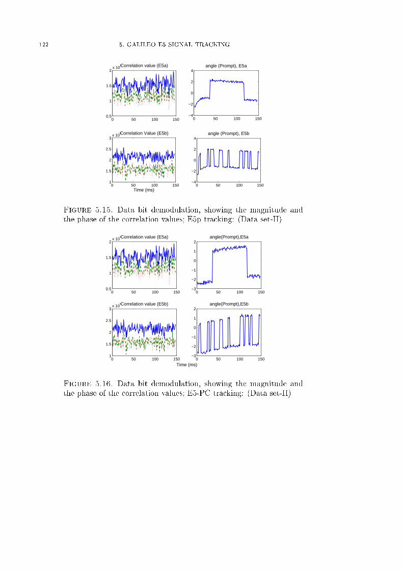
122 5. GALILEO E5 SIGNAL TRACKING
0 50 100 1500.5
1
1.5
2x 10
5Correlation value (E5a)
0 50 100 150−4
−2
0
2
4angle (Prompt), E5a
0 50 100 1501
1.5
2
2.5
3x 10
5
Time (ms)
Correlation Value (E5b)
0 50 100 150−4
−2
0
2
4angle (Prompt), E5b
Figure 5.15. Data bit demodulation, showing the magnitude andthe phase of the correlation values; E5p tracking: (Data set-II)
0 50 100 1500.5
1
1.5
2x 10
5Correlation value (E5a)
0 50 100 150−3
−2
−1
0
1
2angle(Prompt),E5a
0 50 100 1501
1.5
2
2.5
3x 10
5Correlation value (E5b)
0 50 100 150−3
−2
−1
0
1
2angle(Prompt),E5b
Time (ms)
Figure 5.16. Data bit demodulation, showing the magnitude andthe phase of the correlation values; E5-PC tracking: (Data set-II)

5.6. AN EXTENDED TRACKING RANGE DLL 123
−2 −1.5 −1 −0.5 0 0.5 1 1.5 2−0.8
−0.6
−0.4
−0.2
0
0.2
0.4
0.6
0.8
1
Code delay (chips)
Nor
mal
ized
Cor
rela
tion
Val
ue
E5 − UnfilteredE5a/b − UnfilteredE5 −70MHz filterE5a − 20MHz filter
Figure 5.17. Galileo E5 correlation waveform; di�erent �lter bandwidths
of the prompt correlation value shown decodes the data bit as explained earlier.
The data sets were chosen such that the data changes are only in E5b (Data set-I)
and data changes are in both E5a and E5b (Data set-II). The data bit �ip-overs are
indicated by the 180 deg phase jumps in Figs. 5.13-5.16.
5.6. An Extended Tracking Range DLL
In the previous sections, several ways of tracking the AltBOC(15,10) signal were
discussed. Combining the independently processed E5a and E5b correlation re-
sults (through the DSB method or the FIC method) is the best way to maximise
the received signal energy in order to obtain a BPSK(10)-like triangle. Using 8-
PSK-like tracking is the best way to maximise the energy in order to obtain an
AltBOC(15,10) correlation waveform. Fig. 5.17 revisits the correlation plots for
the methods required in this section. In this section, a novel method to combine
the DLL discriminators for the BPSK(10)-like and the AltBOC(15,10) correlation
waveforms is discussed. For the discussion throughout this section, a coherent early
minus late (EML) discriminator has been used due to its simplicity.
5.6.1. DLL considerations. The maximum possible chip spacing assuming
an ideal correlation triangle for 8-PSK tracking is 0.33 chip (this depends on the
bandwidth of the RF front-end �lter). Therefore, an early-late chip spacing of 0.3
is a typical value used in receivers for the 8-PSK tracking, as mentioned in sec. 5.5.
Beyond a 0.3 chip spacing the discriminator has the potential to drive the loop into
a false lock region. Fig. 5.18 shows the S-curve along with the variation of the
S-curve linear region against the chip spacing d for both 8-PSK and BPSK tracking
loops.

124 5. GALILEO E5 SIGNAL TRACKING
−1.5 −1 −0.5 0 0.5 1 1.5−2
−1.5
−1
−0.5
0
0.5
1
1.5
2
Code deay error (chips)
Dis
crim
inat
or o
utpu
t
d = 0.1d = 0.2d = 0.3d = 0.4d = 0.5d = 0.6
−2 −1.5 −1 −0.5 0 0.5 1 1.5 2−0.8
−0.6
−0.4
−0.2
0
0.2
0.4
0.6
0.8
Code delay error (chips)
Dis
crim
inat
or o
utpu
t
d = 0.1
d = 0.2
d = 0.3
d = 0.4
d = 0.5
d = 0.6
Figure 5.18. S-curve for the E5 8-PSK tracking (top) and BPSK(10)tracking for di�erent chip early-late spacing (in�nite bandwidth)
5.6.2. Extended tracking range DLL.
5.6.2.1. The receiver model. In the proposed method, the correlator outputs of
8-PSK and BPSK tracking are combined and are provided as the input to the loop
�lter. Fig. 5.19 shows the receiver model for the proposed architecture. The cor-
relator outputs from the two loops are passed onto a combiner and selector block.
There is only one VCO which updates the timing estimate for both the loops. Note
that the data demodulation is not shown for simpli�cation of the diagram.
5.6.2.2. Discriminator combination. Fig. 5.20 illustrates the regions of interest
of the two discriminators. Consider the 8-PSK tracking loop with 0.3 early-late chip
spacing. For delay errors up to ±0.15 chips, the slope of the S-Curve is positive
and the DLL produces an output to lock to the zero error point. Now consider the
BPSK tracking case. Assume that the chip spacing used for BPSK tracking is 0.6
chips. For delay errors up to ±0.15 chips the slope of the S-curve is positive and
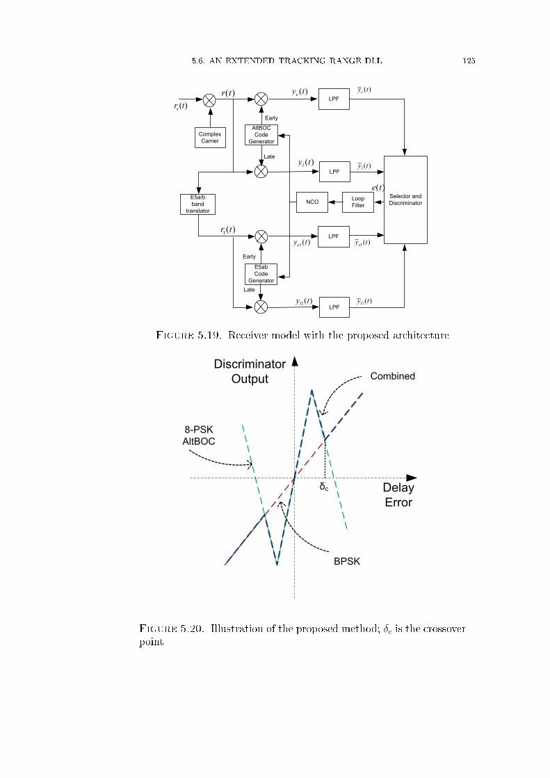
5.6. AN EXTENDED TRACKING RANGE DLL 125
AltBOC
Code
Generator
Complex
Carrier
)(trsLPF
Early
Late
LPF
E5a/b
band
translator
( )ey t
( )ly t
E5ab
Code
Generator
LPF
Early
Late
LPF
1( )ey t
1( )ly t
Selector and
DiscriminatorLoop
FilterNCO
( )e t
1( )r t
( )r t ( )ey t
( )ly t
1( )ey t
1( )ly t
Figure 5.19. Receiver model with the proposed architecture
Discriminator
Output
Delay
Error
8-PSK
AltBOC
BPSK
Combined
δc
Figure 5.20. Illustration of the proposed method; δc is the crossoverpoint

126 5. GALILEO E5 SIGNAL TRACKING
the DLL produces an output to lock to the zero error point. Beyond this chip error,
and up to +/- 0.3 chip error, the DLL for the 8-PSK has negative slope whereas
the BPSK triangle will still have positive slope. The 8-PSK DLL in e�ect may push
the VCO voltage to lock to the secondary peak whereas the BPSK DLL will still
be aiming for the correct central point. Due to the opposite slopes, the two error
outputs cross each other, the 8-PSK discriminator error starts diminishing, but the
BPSK discriminator error will still be growing. Hence the selector block will perform
the following operation:
e(t) =
e0(t) if |e0(t)| < ε
e0(t) if |e0(t)| > Kc |e1(t)|e1(t) if |e0(t)| < Kc |e1(t)|
(5.25)
where
e0(t) = ye(t)− yl(t) (5.26)
e1(t) = ye1(t)− yl1(t) (5.27)
are the individual discriminator outputs of the 8-PSK and BPSK tracking loops
respectively and Kc is the scaling factor which depends on the chip spacing used
for the BPSK discriminator. The parameter ε is added to avoid any unwanted
triggering of the selector at very small discriminator errors, say e0(t) < 0.05. Note
that the delay error corresponding to the crossing point δc depends on the scaling
factor Kc. The error range, for which this algorithm is valid, depends on the chip
spacing used for the BPSK tracking loop (assuming that one always sets the 8-PSK
loop at its typical spacing of 0.3 chips). In addition this algorithm can be extended
for early-late spacing of up to 1.0 chip for the BPSK-triangle.
The advantage in the code tracking range of this method is obvious. Even though
the overall tracking range is controlled by both the DLLs, the output of the BPSK
DLL will be used only rarely, for large displacements. For small displacements,
the 8-PSK loop will take over and the tracking jitter is not a�ected. Others have
addressed a related problem of coming out of the false lock point, for example using
the bump-jumping correlator (Fine and Wilson, 1999) which often requires more
processing by way of having more correlator arms and computing the appropriate
weighting coe�cients for combining them (Fante, 2003).
5.6.3. Performance analysis.
5.6.3.1. Equation for the code tracking jitter of the proposed method. In order to
analyse the proposed algorithm, the code phase tracking jitter is evaluated in terms
of signal and noise components that enter the tracking loop. The performance
analysis of the BPSK and BOC coherent DLLs is given in (Holmes, 2007). Here the

5.6. AN EXTENDED TRACKING RANGE DLL 127
analysis for the extended range method is provided. This linear analysis is valid for
Gaussian input noise. The received spreading waveform (including the sub-carrier)
is denoted here by c(t − τ) where is the τ timing o�set between transmitter and
the receiver. The local spreading waveform is denoted by c(t − τ) where τ is the
receiver estimate of the timing o�set τ . The received signal after the carrier mixing
(assuming a perfect carrier match) in Fig. 5.19 is given by
r(t) =√Pc(t− τ) + nW (t) (5.28)
where P is the signal power and nW (t) is the additive white Gaussian noise with two
sided power spectral density of N0
2Watts/ Hz. Because the signal power in both the
components of the E5a and E5b sidebands is combined, the power loss compared
to the main 8-PSK AltBOC signal is negligible. Hence the same received power
levels at the input of E5a and E5b combined discriminator are assumed. Also the
combined spreading code is represented as c1(t− τ). The input at the E5a and E5b
combined loop is given by
r1(t) =√Pc1(t− τ) + nW (t) (5.29)
The received signal is correlated with the early and late reference waveforms
c(t − τ ± δTc) and c1(t − τ ± δ1Tc) where 2δ = d is the spacing between the early
and late correlator arms for the 8-PSK DLL and 2δ1 = d1 for the BPSK DLL and
Tc denotes the chip period. The code phase error is de�ned as
ε = (τ − τ) (5.30)
Note that a single VCO to adjust the local reference code phase. The correlator
outputs are given by:
ye(t) =√Pc(t− τ)c(t− τ + δTc) + nW (t)c(t− τ + δTc) (5.31)
yl(t) =√Pc(t− τ)c(t− τ − δTc) + nW (t)c(t− τ − δTc) (5.32)
ye1(t) =√Pc(t− τ)c1(t− τ + δ1Tc) + nW (t)c1(t− τ + δ1Tc) (5.33)
yl1(t) =√Pc(t− τ)c1(t− τ − δ1Tc) + nW (t)c1(t− τ − δ1Tc) (5.34)
Assuming that the autocorrelation noise and the correlation noise between indi-
vidual codes are negligible, the output of the LPF yields:
ye/l(t) =√PR(τ − τ ± δTc) + ne/l(t)
=√PR(ε± δTc) + ne/l(t) (5.35)
ye1/l1(t) =√PR1(τ − τ ± δ1Tc) + ne1/l1(t)
=√PR1(ε± δ1Tc) + ne1/l1(t) (5.36)
where R(•) and R1(•) are the correlation functions of 8-PSK AltBOC and BPSK

128 5. GALILEO E5 SIGNAL TRACKING
respectively. The selection algorithm now chooses the error value according to (5.25).
Hence
e(t) =
√PD(ε) + n′(t) 0 6 |ε| < δc√PD1(ε) + n′1(t) δc 6 |ε| < δ1
(5.37)
where D(ε) is the discriminator error function. Note that because no additional
noise components are added in the selection process, the noise in the two cases will
comprise only two noise components. The two-sided power spectral density of the
resultant noise at f = 0 is given by (Holmes, 2007)
Sn′1(0) = N0 [1−R1(2δ1Tc)] = N0d1 (5.38)
Sn′(0) = N0 [1−R(2δTc)] = N0 [1−R(dTc)] (5.39)
The code tracking jitter is given by (Holmes, 2007)
σ2ε =
N0 · 2BL [1−R(dTc)]
PK2(5.40)
where BL is the one-sided closed-loop noise bandwidth of the code-tracking loop
and K is the slope if the discriminator curve. Since a closed form expression for the
AltBOC correlation function does not exist to the authors' knowledge, as mentioned
in sec. 2.4, the correlation function is retained as it is and computed during the
simulation process. The code tracking jitter is then given by
σ2ε =
N0BL1d12P
forBPSK
N0·BL[1−R(dTc)]PK2 for 8-PSK AltBOC
where BL and BL1 are the corresponding code lock loop �lter bandwidths. For the
AltBOC(15,10) signal with 70 MHz front-end �lter bandwidth and d= 0.3, the value
of K is found to be 9 and [1−R(dTc)] ≈ 0.4.
Only outside the region {−δc,+δc}, is the code tracking jitter of the BPSK valid.
As soon as the loop has errors less than ±δc, one obtains a smaller jitter dictated
by the 8-PSK loop. Note that for delay errors from ±δ to ±δc the jitter will be
slightly more than that in the linear region because the slope of the discriminator
curve is slightly less. Since the scaling factor Kc controls δc, Kc can be adjusted (for
a given δ and δ1 ) for a given design and will not be discussed in this chapter. A
coherent EML discriminator with δ=0.15 and a value of Kc=3 gives δc≈0.2. It doesnot depend on δ1 as the slope of the BPSK coherent EML discriminator does not
depend on the chip spacing.
5.6.3.2. Results. The proposed algorithm has been tested on the Galileo In-Earth
Orbit Validation Equipment (GIOVE) satellite E5 signal collected using the Septen-
trio GeNeRx1 receiver. Since the existing setup is bench test equipment, errors in
the estimated code delay have been added during the simulations to make the loop

5.6. AN EXTENDED TRACKING RANGE DLL 129
0 50 100 150−0.5
0
0.5
Cod
e ph
ase
erro
r (c
hips
)
0 50 100 1505
6
7
8
Cod
e D
oppl
er (
Hz)
0 50 100 1500.5
1
1.5
2
2.5x 10
5
Cor
rela
tion
valu
e
Time (ms)
Figure 5.21. 8-PSK AltBOC tracking without introducing any error
0 50 100 150−0.5
0
0.5
Cod
e ph
ase
erro
r (c
hips
)
0 50 100 1505
6
7
8C
ode
Dop
pler
(H
z)
0 50 100 1500
0.5
1
1.5
2
2.5x 10
5
Cor
rela
tion
valu
e
Time (ms)
Figure 5.22. BPSK(10) E5ab tracking without introducing any error
deviate from normal behaviour.
Figs. 5.21 and 5.22 show the code tracking without any errors induced during
testing. The bottom portion of the �gure shows the early (green, -*-), prompt (blue,
�) and late (red, -�-) correlation values. When an error is introduced from 60-105
ms and 8-PSK tracking is used, then the result is as shown in Fig. 5.23. Note that
the code lock loop is diverging. With the proposed method shown in Fig. 5.24, the
code lock loop caters for this change and pulls the loop back to the proper code
Doppler and hence the code phase error remains small.

130 5. GALILEO E5 SIGNAL TRACKING
0 50 100 150−1
−0.5
0
0.5
1
Cod
e ph
ase
erro
r (c
hips
)
0 50 100 1504
6
8
10
Cod
e D
oppl
er (
Hz)
0 50 100 1500
0.5
1
1.5
2
2.5x 10
5
Cor
rela
tion
valu
e
Time (ms)
Figure 5.23. 8-PSK AltBOC tracking; error introduced from 60-105 ms
0 50 100 150−1
−0.5
0
0.5
1
Cod
e ph
ase
erro
r (c
hips
)
0 50 100 1504
6
8
10
Cod
e D
oppl
er (
Hz)
0 50 100 1500.5
1
1.5
2
2.5x 10
5
Cor
rela
tion
valu
e
Time (ms)
Figure 5.24. 8-PSK AltBOC tracking with the hybrid DLL method;error introduced from 60-105 ms

5.7. SUMMARY 131
5.7. Summary
This chapter discussed several tracking architectures that are possible for track-
ing the E5 signal and its components by making use of di�erent local reference
signals. The advantages and disadvantages of using di�erent reference signals are
discussed and a pre-correlation combination type of hybrid tracking architecture is
described. Performance of the proposed architecture was analysed, and real sig-
nal tracking results for GIOVE-A were obtained. In summary, the two preferred
tracking methods are the quasi-coherent E5 and the proposed pre-correlation com-
bination method. The quasi-coherent E5 tracking tops the performance but requires
12 sets of code mixers and accumulators. In addition, longer coherent integration in
the quasi-coherent E5 architecture has a weak link due to the �max� operation that
helps perform the data wipe-o� operation. The performance of the pre-correlation
combination architecture is 18% inferior to the quasi-coherent E5 architecture. How-
ever, the pre-correlation combination method requires only 5 sets of code mixers and
accumulators (less than half compared to the quasi-coherent E5 architecture), and
also allows longer coherent integration beyond beyond one data bit duration. Hence
the pre-correlation combination is useful in situations where the correlator resources
are limited (or if there is a requirement of low power consumption).
This chapter also proposed a new method of increasing the e�ective tracking
range for code tracking of AltBOC signals without a�ecting the jitter performance
in the existing linear range of the code tracking loop. By selecting the appropriate
discriminator output between the BPSK tracking loop and the 8-PSK tracking loop,
it is shown that errors larger than the linear tracking range of the 8-PSK tracking
loop can be pulled back to the linear region without any degradation in the tracking
jitter. The proposed algorithm can be used in systems where there is a possibility
of obtaining a wider and narrower correlation triangle for a given signal.


CHAPTER 6
Galileo E5 Code Phase Multipath Mitigation
6.1. Introduction
This chapter proposes a method to mitigate the code phase multipath by ex-
ploiting the frequency diversity which is inherent to the AltBOC modulation used
in Galileo E5 satellite navigation signals. The �rst part of this chapter deals with the
multipath mitigation technique in detail and the second part introduces the group
delay compensation viewpoint for the proposed frequency diversity based multi-
path mitigation scheme. Sec. 6.2 to sec. 6.4 contain the work published in ION
GNSS 2009 (Shivaramaiah, 2009)(student paper sponsorship award winner and best
presentation award winner in the session). This work is also a part of the patent
(Shivaramaiah and Dempster, 2009b) handled by NewSouth Innovations Pty Lim-
ited (NSi), a wholly owned subsidiary and controlled entity of University of New
South Wales (UNSW). Sec. 6.5 contains the work published in IEEE/ION PLANS
2010 (Shivaramaiah and Dempster, 2010a).
In sec. 6.2, the multipath performance of the Galileo E5 Direct AltBOC sig-
nal tracking architecture (presented in chapter 5) is discussed. In sec. 6.3, the
proposed multipath mitigation scheme, called the Sideband Carrier Phase Combi-
nation (SCPC) method, is described with the associated tracking loop architecture.
Sec. 6.4 presents the simulation and test results for the SCPC. Sec. 6.5 discusses
the group delay compensation viewpoint for the frequency diversity based multipath
mitigation scheme. Section 6.6 summarises the contents of this chapter.
6.2. Performance of the Direct AltBOC Tracking Architecture
6.2.1. Model of the received signal. The received E5 AltBOC signal of any
one satellite in the presence of a direct signal and N re�ected components can be
represented as:
rIF (t) =N∑i=0
√2aiP · <
[s (t− ti) · ej(ωIF t+ωdi t+θi)
]+ nW (t) (6.1)
where s(t) = sc(t)+jss(t) is the complex baseband signal, ωIF and ωd are the carrier
and Doppler frequencies respectively, θi is the phase, ti is the delay and ai is the
attenuation of the ith signal, P is the received signal power, nW (t) is the additive
white Gaussian noise, and < is the real argument function. For most applications,
133

134 6. GALILEO E5 CODE PHASE MULTIPATH MITIGATION
it can be assumed that the di�erence in Doppler between the direct signal and the
re�ected signals is negligible (especially for delays less than one chip of the Galileo
E5 spreading code). The attenuation, time delay and phase of each signal can be
written relative to that of the direct component as:
αi =aia0
, τi = ti − t0 , φi = |θi − θ0|2π (6.2)
Letting ω0 = ωIF + ωd, (G.1) can then be written as:
rIF (t) =N∑i=0
√2aiP ·
(sc (t− t0 − τi) · cos (ω0t+ θ0 + φi)−ss (t− t0 − τi) · sin (ω0t+ θ0 + φi)
)+ nW (t) (6.3)
6.2.2. Signal tracking with the Direct AltBOC architecture. Signal track-
ing in Galileo E5 receivers can be achieved in several ways as discussed in Chapter
5. Two major techniques are important in the context of this chapter. One is the
wideband signal tracking, where the received signal is passed through a wideband
�lter (at least 51.15 MHz bandwidth so as to pass the two dominant lobes) centred
around 1191.795 MHz. This type of tracking allows full utilisation of the shape of
the AltBOC correlation function and the received power and has been termed Direct
AltBOC tracking in Chapter 5 (also referred to as 8-PSK AltBOC tracking). The
second is side-band tracking, where the E5a and E5b sidebands are extracted from
the received signal by multiplying it with an appropriate complex sub-carrier. Since
this operation results in a BPSK(10)-like correlation function, it is also referred to
as BPSK(10) tracking. The same terminologies are retained in this chapter.
The generalised tracking architecture presented in Chapter 5 for the Galileo E5
signal is shown again in Fig. 6.1. In Fig. 6.1, all the lines with x, s and y as the label
carry complex signals. The reference signals are the early, late and prompt versions
of the AltBOC signal with a spacing of 2δ chips between early and late samples:
s∗1(t− τ) = s∗(t− τ + δTc) (6.4a)
s∗2(t− τ) = s∗(t− τ − δTc) (6.4b)
s∗0(t− τ) = s∗(t− τ) (6.4c)
where Tc is the chip duration.
6.2.3. Code tracking error in the presence of multipath, without noise.
In accordance with the customary method used in Holmes (2007) and Braasch (1996)
a single re�ected signal without noise is assumed in order to derive an equation for
the discriminator function, and hence to analyse the e�ect of multipath on the
code tracking error. The discriminator function in the presence of a single re�ected
signal for the coherent early-minus-late (CEML) discriminator is given by (derived
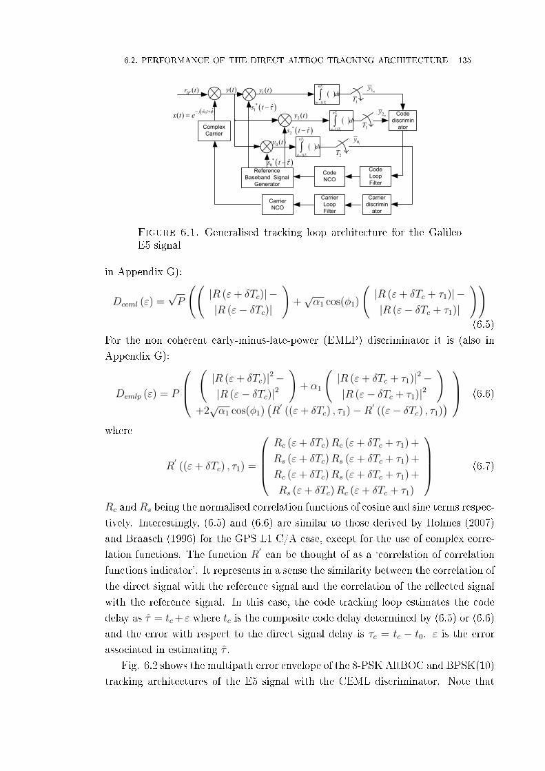
6.2. PERFORMANCE OF THE DIRECT ALTBOC TRACKING ARCHITECTURE 135
Reference
Baseband Signal
Generator
Complex
Carrier
( )IFr t
Code
Loop
Filter
Code
NCO
1my
1( )y t
2 ( )y t 0
ˆˆ
( )j t
x t e
( )y t
1
1( 1)
nT
n T
dt
1T
1T
2my
*
1ˆs t
*
2ˆs t
*
0ˆs t
Carrier
Loop
Filter
Carrier
discrimin
ator
Carrier
NCO
0 ( )y t
2
2( 1)
nT
n T
dt
0ly
2T
1
1( 1)
nT
n T
dt
Code
discrimin
ator
Figure 6.1. Generalised tracking loop architecture for the GalileoE5 signal
in Appendix G):
Dceml (ε) =√P
((|R (ε+ δTc)| −|R (ε− δTc)|
)+√α1 cos(φ1)
(|R (ε+ δTc + τ1)| −|R (ε− δTc + τ1)|
))(6.5)
For the non coherent early-minus-late-power (EMLP) discriminator it is (also in
Appendix G):
Demlp (ε) = P
(|R (ε+ δTc)|2−|R (ε− δTc)|2
)+ α1
(|R (ε+ δTc + τ1)|2−|R (ε− δTc + τ1)|2
)+2√α1 cos(φ1)
(R′((ε+ δTc) , τ1)−R′ ((ε− δTc) , τ1)
) (6.6)
where
R′((ε+ δTc) , τ1) =
Rc (ε+ δTc)Rc (ε+ δTc + τ1) +
Rs (ε+ δTc)Rs (ε+ δTc + τ1) +
Rc (ε+ δTc)Rs (ε+ δTc + τ1) +
Rs (ε+ δTc)Rc (ε+ δTc + τ1)
(6.7)
Rc and Rs being the normalised correlation functions of cosine and sine terms respec-
tively. Interestingly, (6.5) and (6.6) are similar to those derived by Holmes (2007)
and Braasch (1996) for the GPS L1 C/A case, except for the use of complex corre-
lation functions. The function R′can be thought of as a `correlation of correlation
functions indicator'. It represents in a sense the similarity between the correlation of
the direct signal with the reference signal and the correlation of the re�ected signal
with the reference signal. In this case, the code tracking loop estimates the code
delay as τ = tc+ ε where tc is the composite code delay determined by (6.5) or (6.6)
and the error with respect to the direct signal delay is τc = tc − t0. ε is the errorassociated in estimating τ .
Fig. 6.2 shows the multipath error envelope of the 8-PSK AltBOC and BPSK(10)
tracking architectures of the E5 signal with the CEML discriminator. Note that

136 6. GALILEO E5 CODE PHASE MULTIPATH MITIGATION
0 10 20 30 40 50 60−3
−2
−1
0
1
2
3
Multipath delay (m)
Cod
e m
ultip
ath
erro
r (m
)
Code multipath error comparison, SMR = 6dB
E5a−20MHz; δ=0.15E5−50MHz; δ=0.15
Figure 6.2. Code multipath error envelope of E5a and E5 correlatorswith CEML discriminator
Direct AltBOC tracking with at least 50 MHz bandwidth performs better than the
E5a tracking with 20 MHz bandwidth (5th order Butterworth �lters have been used).
However, there is still scope for improvement for multipath delays less than 20 m,
if the goal (say) is to bring the multipath error down to 0.5 m or less.
6.2.4. Carrier phase error in the presence of multipath and code phase
multipath error, without noise. The concepts developed for carrier phase error
for the other signals also valid for the E5 AltBOC tracking architectures. This is
because as far as the carrier is concerned, there is no change in the signal structure
except that they are at di�erent frequencies. In the absence of multipath, the carrier
lock loop estimates the carrier phase φ = θ0 + εφ where εφ is the error associated
with the estimate. In the presence of multipath, the carrier lock loop estimates the
carrier phase θc of the composite signal. The carrier phase multipath error for the
AltBOC signal consisting of direct signal component and a single re�ected signal
component is given by (derived in Appendix (H)):
φc = arctan
( √α1 |R (ε+ τ1)| sin (φ1)
|R (ε)|+√α1 |R (ε+ τ1)| cos (φ1)
)(6.8)
where φc = θc−θ0 is the phase error (which is the same as the phase of the composite
signal when θ0 = 0), and again R is the complex autocorrelation function between
the input signal and the reference signal. Note that the carrier phase error depends
on the error in estimating the code phase .
The carrier phase multipath error envelope is shown in Fig. 6.3. Observe that
unlike the case for BPSK tracking both the code and carrier phase errors have nulls
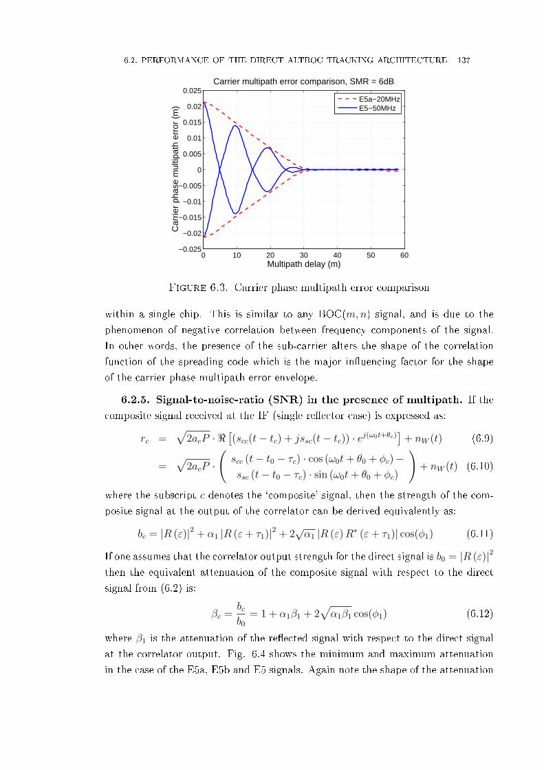
6.2. PERFORMANCE OF THE DIRECT ALTBOC TRACKING ARCHITECTURE 137
0 10 20 30 40 50 60−0.025
−0.02
−0.015
−0.01
−0.005
0
0.005
0.01
0.015
0.02
0.025
Multipath delay (m)
Car
rier
phas
e m
ultip
ath
erro
r (m
)
Carrier multipath error comparison, SMR = 6dB
E5a−20MHzE5−50MHz
Figure 6.3. Carrier phase multipath error comparison
within a single chip. This is similar to any BOC(m,n) signal, and is due to the
phenomenon of negative correlation between frequency components of the signal.
In other words, the presence of the sub-carrier alters the shape of the correlation
function of the spreading code which is the major in�uencing factor for the shape
of the carrier phase multipath error envelope.
6.2.5. Signal-to-noise-ratio (SNR) in the presence of multipath. If the
composite signal received at the IF (single re�ector case) is expressed as:
rc =√
2acP · <[(scc(t− tc) + jssc(t− tc)) · ej(ω0t+θc)
]+ nW (t) (6.9)
=√
2acP ·(scc (t− t0 − τc) · cos (ω0t+ θ0 + φc)−ssc (t− t0 − τc) · sin (ω0t+ θ0 + φc)
)+ nW (t) (6.10)
where the subscript c denotes the `composite' signal, then the strength of the com-
posite signal at the output of the correlator can be derived equivalently as:
bc = |R (ε)|2 + α1 |R (ε+ τ1)|2 + 2√α1 |R (ε)R∗ (ε+ τ1)| cos(φ1) (6.11)
If one assumes that the correlator output strength for the direct signal is b0 = |R (ε)|2then the equivalent attenuation of the composite signal with respect to the direct
signal from (6.2) is:
βc =bcb0
= 1 + α1β1 + 2√α1β1 cos(φ1) (6.12)
where β1 is the attenuation of the re�ected signal with respect to the direct signal
at the correlator output. Fig. 6.4 shows the minimum and maximum attenuation
in the case of the E5a, E5b and E5 signals. Again note the shape of the attenuation

138 6. GALILEO E5 CODE PHASE MULTIPATH MITIGATION
0 50 100 150 200 250 300 3500
0.5
1
1.5
E5a
Minimum attenuation and maximum amplification, SMR = 6dB
0 50 100 150 200 250 300 3500
0.5
1
1.5
E5b
0 50 100 150 200 250 300 3500
0.5
1
1.5
E5
Multipath delay (decimeter)
Figure 6.4. Envelope of the attenuation (normalised ratio) for E5a,E5b, and E5 signals under multipath conditions
for E5, which is due to the shape of the correlation function.
6.3. SCPC Method and an Architecture
6.3.1. E5a and E5b carrier phases under multipath. The E5a, E5 and
E5b signals have wavelengths of λE5a=25.48 cm, λE5=25.15 cm and λE5b=24.83
cm respectively, due to their corresponding carrier frequencies. When the signal
travels from the satellite to the receiver, a certain number of cycles plus a fraction
of a cycle elapse. This fraction of a cycle converted to radians is the phase of the
received signal i.e. θ = 2πdλ
where d is the distance between the transmitter and the
receiver. In the absence of re�ected signals, the phase of the received signal depends
on the distance between the satellite and the receiver plus any associated errors in
estimating the pseudorange. Denote the phase of the received signals in this case
for E5, E5a and E5b as θ0 = 2πdλE5
, θ0a = 2πdλE5a
and θ0b = 2πdλE5b
respectively. In the
presence of multipath, there can be any number of re�ected signals. In this thesis
only the single re�ection case is considered. However, the method described in this
chapter applies equally well to the case where there are more than one re�ected
signals arriving at the receiver antenna.
The re�ected signal always arrives after the direct signal. This means that the
re�ected signal always travels a longer distance than the direct signal. If the distance
travelled by the re�ected signal is d1(> d) then the phases of the re�ected signal
will be θ1 = 2πd1λE5
, θ1a = 2πd1λE5a
and θ1b = 2πd1λE5b
. The multipath delay, which is nothing
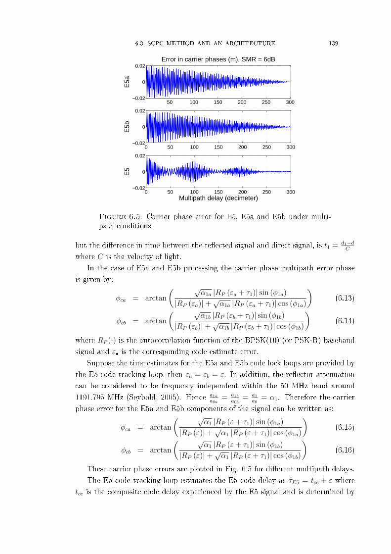
6.3. SCPC METHOD AND AN ARCHITECTURE 139
50 100 150 200 250 300−0.02
0
0.02
E5a
Error in carrier phases (m), SMR = 6dB
0 50 100 150 200 250 300−0.02
0
0.02
E5b
0 50 100 150 200 250 300−0.02
0
0.02
E5
Multipath delay (decimeter)
Figure 6.5. Carrier phase error for E5, E5a and E5b under multi-path conditions
but the di�erence in time between the re�ected signal and direct signal, is t1 = d1−dC
where C is the velocity of light.
In the case of E5a and E5b processing the carrier phase multipath error phase
is given by:
φca = arctan
( √α1a |RP (εa + τ1)| sin (φ1a)
|RP (εa)|+√α1a |RP (εa + τ1)| cos (φ1a)
)(6.13)
φcb = arctan
( √α1b |RP (εb + τ1)| sin (φ1b)
|RP (εb)|+√α1b |RP (εb + τ1)| cos (φ1b)
)(6.14)
where RP (·) is the autocorrelation function of the BPSK(10) (or PSK-R) baseband
signal and ε• is the corresponding code estimate error.
Suppose the time estimates for the E5a and E5b code lock loops are provided by
the E5 code tracking loop, then εa = εb = ε. In addition, the re�ector attenuation
can be considered to be frequency independent within the 50 MHz band around
1191.795 MHz (Seybold, 2005). Hence a1aa0a
= a1ba0b
= a1a0
= α1. Therefore the carrier
phase error for the E5a and E5b components of the signal can be written as:
φca = arctan
( √α1 |RP (ε+ τ1)| sin (φ1a)
|RP (ε)|+√α1 |RP (ε+ τ1)| cos (φ1a)
)(6.15)
φcb = arctan
( √α1 |RP (ε+ τ1)| sin (φ1b)
|RP (ε)|+√α1 |RP (ε+ τ1)| cos (φ1b)
)(6.16)
These carrier phase errors are plotted in Fig. 6.5 for di�erent multipath delays.
The E5 code tracking loop estimates the E5 code delay as τE5 = tcc + ε where
tcc is the composite code delay experienced by the E5 signal and is determined by

140 6. GALILEO E5 CODE PHASE MULTIPATH MITIGATION
50 100 150 200 250 300−2
0
2
E5a
Error in pseudorange (m), SMR = 6dB
50 100 150 200 250 300−2
0
2
E5b
50 100 150 200 250 300−2
0
2
E5
Multipath delay (decimeter)
Figure 6.6. Code pseudorange error for E5, E5a and E5b undermultipath conditions
(6.5). The error with respect to the E5 direct signal delay is τcc = tcc − t0. The
E5a code tracking loop estimates the E5a code delay as τE5a = tca + εa where tca is
the composite code delay experienced by the E5a signal and is determined by the
real component of (6.5). The error with respect to the E5a direct signal delay is
τca = tca − t0. Similarly, for the E5b signal, τE5b = tcb + εb and τcb = tcb − t0. With
the SCPC architecture, as mentioned earlier, ε = εa = εb. Hence τcc = τE5−(t0 +ε),
τca = τE5a − (t0 + ε) and τcb = τE5b − (t0 + ε). The code phase error thus calculated
due to multipath is plotted in Fig. 6.6 for E5, E5a and E5b for di�erent multipath
delays.
In these simulations, without loss of generality, it is assumed that the phase
change of the re�ected signal is only due to the path delay (usually, the phase is
inverted upon re�ection). In addition, the phase change is considered to be constant
over the entire E5 band. This is a reasonable assumption since the re�ectors are
negligibly dispersive within 50 MHz at around 1.2 GHz (Seybold, 2005). Other error
sources are discussed later in the chapter. If the carrier phase errors in (6.8), (6.15)
and (6.16) are subtracted from each other, then the results obtained are as shown
in Fig. 6.7.
The shape of the di�erence in carrier phase errors resembles the shape of the
code phase multipath error of the E5 signal. If one again subtracts the code phase
error from this di�erence in carrier phases, then the results shown in Fig. 6.8 are
obtained. The subtraction is formulated as follows:
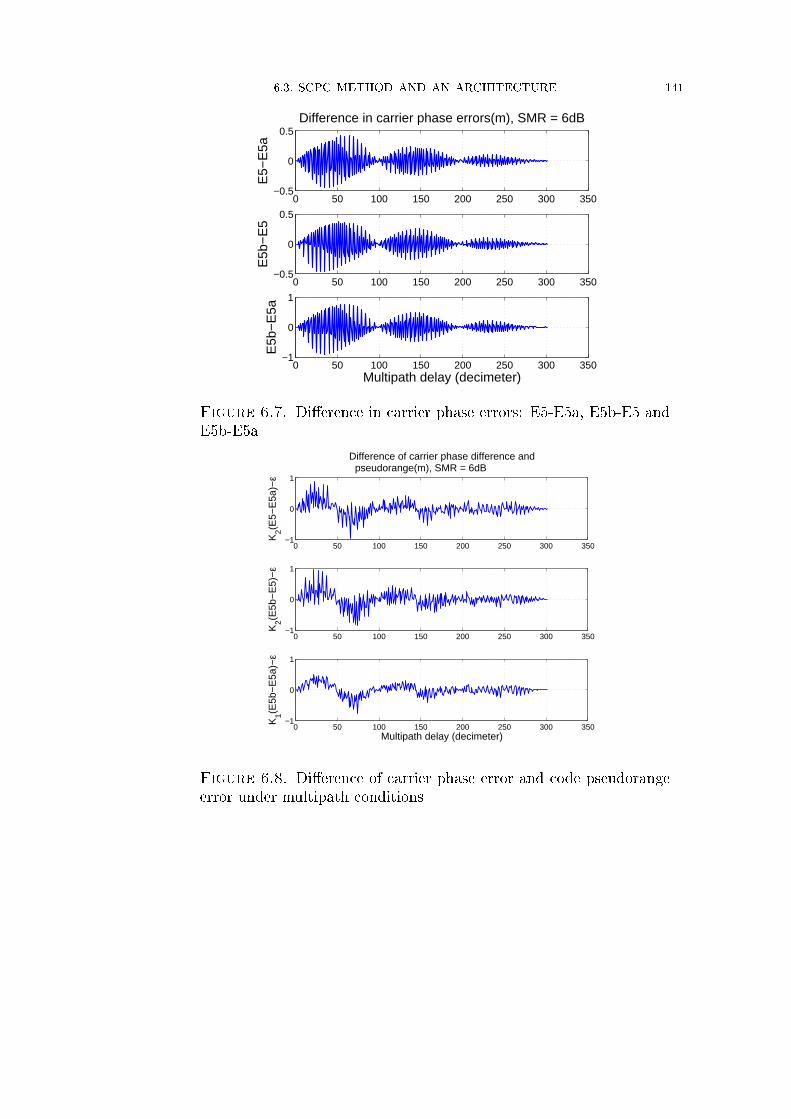
6.3. SCPC METHOD AND AN ARCHITECTURE 141
0 50 100 150 200 250 300 350−0.5
0
0.5
E5−
E5a
Difference in carrier phase errors(m), SMR = 6dB
0 50 100 150 200 250 300 350−0.5
0
0.5
E5b
−E
5
0 50 100 150 200 250 300 350−1
0
1
E5b
−E
5a
Multipath delay (decimeter)
Figure 6.7. Di�erence in carrier phase errors: E5-E5a, E5b-E5 andE5b-E5a
0 50 100 150 200 250 300 350−1
0
1
K2(E
5−E
5a)−
ε
Difference of carrier phase difference and pseudorange(m), SMR = 6dB
0 50 100 150 200 250 300 350−1
0
1
K2(E
5b−
E5)
−ε
0 50 100 150 200 250 300 350−1
0
1
K1(E
5b−
E5a
)−ε
Multipath delay (decimeter)
Figure 6.8. Di�erence of carrier phase error and code pseudorangeerror under multipath conditions

142 6. GALILEO E5 CODE PHASE MULTIPATH MITIGATION
0 50 100 150 200 250 300 3500.5
1
1.5
E5a
Composite Signal Strength (normalized ratio), SMR = 6dB
0 50 100 150 200 250 300 3500.5
1
1.5
E5b
0 50 100 150 200 250 300 3500
0.5
1
1.5
E5
Multipath delay (decimeter)
Figure 6.9. Multipath a�ected signal strength for E5, E5a and E5bsignals
εab = τc −K1 (φcb − φca)εbc = τc −K2 (φbc − φc) (6.17)
εca = τc −K2 (φc − φca)
The resulting values εab, εbc and εca plotted in Fig. 6.8 show that the code phase
multipath errors are reduced to a signi�cant extent if these for the measurements
are used. The optimum value of the constants K1 and K2 depends on the receiver
bandwidth. In addition K2 = 2K1. Typically, the value of is found to be around 2.0
(experimentally determined).
6.3.2. E5a and E5b SNRs under multipath. Consider the received signal
consisting of a single re�ected signal as described in (6.9). The receiver processing
the signal a�ected by multipath estimates the SNR as the composite SNR instead
of the SNR of the direct signal. In the case of E5, E5a and E5b processing, this
SNR is given by:
bca = R2P (ε) + α1R
2P (ε+ τ1) + 2
√α1RP (ε)RP (ε+ τ1) cos(φ1a) (6.18)
bcb = R2P (ε) + α1R
2P (ε+ τ1) + 2
√α1RP (ε)RP (ε+ τ1) cos(φ1b) (6.19)
where bca is the SNR of the composite signal as seen at the E5a band and bcb is
the SNR of the composite signal as seen at the E5a band. The equations (6.11),
(6.18) and (6.19) show that the composite signal strengths di�er among the three
signals and the di�erence is only related to the phase of the multipath signal. These
composite SNRs are plotted in Fig. 6.9 for di�erent multipath delays.
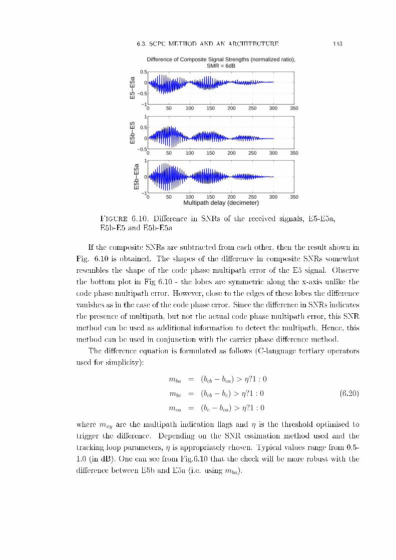
6.3. SCPC METHOD AND AN ARCHITECTURE 143
0 50 100 150 200 250 300 350−1
−0.5
0
0.5
E5−
E5a
Difference of Composite Signal Strengths (normalized ratio), SMR = 6dB
0 50 100 150 200 250 300 350−0.5
0
0.5
1
E5b
−E
5
0 50 100 150 200 250 300 350−1
0
1
E5b
−E
5a
Multipath delay (decimeter)
Figure 6.10. Di�erence in SNRs of the received signals, E5-E5a,E5b-E5 and E5b-E5a
If the composite SNRs are subtracted from each other, then the result shown in
Fig. 6.10 is obtained. The shapes of the di�erence in composite SNRs somewhat
resembles the shape of the code phase multipath error of the E5 signal. Observe
the bottom plot in Fig 6.10 - the lobes are symmetric along the x-axis unlike the
code phase multipath error. However, close to the edges of these lobes the di�erence
vanishes as in the case of the code phase error. Since the di�erence in SNRs indicates
the presence of multipath, but not the actual code phase multipath error, this SNR
method can be used as additional information to detect the multipath. Hence, this
method can be used in conjunction with the carrier phase di�erence method.
The di�erence equation is formulated as follows (C-language tertiary operators
used for simplicity):
mba = (bcb − bca) > η?1 : 0
mbc = (bcb − bc) > η?1 : 0 (6.20)
mca = (bc − bca) > η?1 : 0
where mxy are the multipath indication �ags and η is the threshold optimised to
trigger the di�erence. Depending on the SNR estimation method used and the
tracking loop parameters, η is appropriately chosen. Typical values range from 0.5-
1.0 (in dB). One can see from Fig.6.10 that the check will be more robust with the
di�erence between E5b and E5a (i.e. using mba).

144 6. GALILEO E5 CODE PHASE MULTIPATH MITIGATION
AltBOC Ref
Signal Generator
Complex
Carrier
( )IFr t
Code
Loop
Filter
Code
NCO
1my
1( )y t
2 ( )y t 0
ˆˆ
( )j t
x t e
( )y t
1
1( 1)
nT
n T
dt
1T
1T
2my
*
5ˆ
E cs t T
*
5ˆ
E cs t T
*
5ˆ
Es t
Carrier
Loop
Filter
Carrier
discrimin
ator
Carrier
NCO
0 ( )y t
2
2( 1)
nT
n T
dt
0ly
2T
1
1( 1)
nT
n T
dt
Code
discrimin
ator
E5a/b
band
translator
E5a and E5b
Code Generator
*
5ˆ
E as t *
5ˆ
E bs t
Carrier
Loop Filter
(E5b)
Carrier
discrimin
ator(E5b)
E5b
Carrier
NCO
0 ( )by t
2
2( 1)
nT
n T
dt
0by
2T
2
2( 1)
nT
n T
dt
0ay
2T
Carrier
Loop Filter
(E5a)
Carrier
discrimin
ator(E5a)
E5a
Carrier
NCO
0 ( )ay t Combiner
c
ca
cb
Code phase
measurement
cb cab cbb
Figure 6.11. Architecture for the SCPC method
6.3.3. Architecture for the SCPC method. The required architecture for
the SCPC method is illustrated in Fig. 6.11. Note that this is a special case of the
generalised architecture presented in chapter (5). Important points to observe are
that the code delay estimate from the output of the code NCO used for E5 tracking
is input to the E5a and E5b code generators (indicated by a bold blue line). No
additional code NCOs are required for the E5a and E5b signals because the timing
for both the 8-PSK AltBOC reference signal and the E5a/b code generator are the
same. In fact, the outputs of the E5a/b code generator shown explicitly in this
diagram are already available in the AltBOC reference signal generator and hence
additional hardware is not required except for the code mixers and loop modules.
The combiner block performs the scaled di�erence of the carrier phases according
to (6.17). In (6.17) it can be seen that this scaled di�erence of carrier phases
represents the code multipath delay error. Therefore when the scaled di�erence is
subtracted from the code delay estimate τ , one obtains the multipath mitigated
code delay measurement. The carrier phase errors are obtained via the loop �lters.
In addition, the measured SNRs at the output of the E5, E5a and E5b loops are
provided as input to the combiner block. This is used to gate the subtraction of
the scaled di�erence from the code delay estimate. A method to estimate the signal
strength parameter is to average the squared magnitude of the prompt correlator
output y0 of the corresponding signal component (not shown here).
6.3.4. Explaining the SCPC method. The �ltered correlation function of
the AltBOC(15,10) can be approximated as the product of a symmetrical triangle

6.3. SCPC METHOD AND AN ARCHITECTURE 145
−3 −2 −1 0 1 2 3−1
−0.8
−0.6
−0.4
−0.2
0
0.2
0.4
0.6
0.8
1
Time delay (primary code chips)
Pro
duct
of t
he tr
iang
ular
and
sin
e w
avef
orm
s
cos(2π fsc
t)
ACF of E5aACF of E5
Figure 6.12. Illustrating the formation of the 8PSK / AltBOC-likecorrelation function
−2 −1.5 −1 −0.5 0 0.5 1 1.5 2−1
−0.8
−0.6
−0.4
−0.2
0
0.2
0.4
0.6
0.8
1
Time delay (chips)Pro
duct
of t
he tr
iang
ular
and
sin
e w
avef
orm
s
cos(2π fsc
t)
cos(2π fsc
t−π/2)
cos(2π fsc
t+π/2)
Figure 6.13. Illustrating the e�ect of phase shift while multiplyinga sine wave and a triangle
of width two chips and a cosine wave at a frequency fsc Hz as shown in Fig. 6.12.
Of course the shape of the correlation function depends on the RF front-end �lter
parameters, nevertheless this is a good approximation.
Note that the sine wave is such that its zero phase corresponds to the zero delay
error. If the phase of the sine wave is advanced or retarded by π2then interestingly
the resulting waveform resembles the coherent early-late and late-early discriminator
S-curves with δ=0.167. This is shown in Fig. 6.13. The zero crossings are at zero
delay error and can be thought of as the case without multipath.
If the phase of the cosine wave is not zero, then the shape of the resultant
waveform is changed. This is shown in Fig. 6.14 for di�erent phase shifts from −π2

146 6. GALILEO E5 CODE PHASE MULTIPATH MITIGATION
−1 −0.5 0 0.5 1−1
−0.8
−0.6
−0.4
−0.2
0
0.2
0.4
0.6
0.8
1
Time delay (chips)
Pro
duct
of t
he tr
iang
ular
and
sin
e w
avef
orm
s
−π/2−3π/8−π/4−π/80+π/8+π/4+3π/2+π/2
Figure 6.14. Illustration of the e�ect of di�erent phase shifts of thesine wave due to the multiplication
to +π2. Observe that for phase shifts other than ±π
2, the zero crossing does not align
with the zero delay error. These zero crossings can be thought of as representing
the discriminator S-curve with multipath.
Now consider the equation for the carrier phase multipath error for E5a and
E5b given in 6.15, 6.16. The numerator contains the expression of a PSK-R(10)
correlation function multiplied by a sine function. The multipath phase relations
can be written as:
φ1a = φ1 − φscφ1b = φ1 + φsc
where φsc = 2πfscτ1 is the phase shift induced by the sub-carrier.
Note that the phase di�erences are less a�ected by a small change in the multi-
path delay because the beat frequencies have a wavelength of ~20 metres (E5-E5a,
E5b-E5) and ~10 metres (E5b-E5a). For E5a:
RP (ε+ τ1) sin (φ1a) =√α1RP (ε+ τ1) sin (φ1 − φsc)
=√α1RP (ε+ τ1) (sin (φ1) cos (φsc)− cos (φ1) sin (φsc)) (6.21)
For E5b:
RP (ε+ τ1) sin (φ1b) =√α1RP (ε+ τ1) sin (φ1 + φsc)
=√α1RP (ε+ τ1) (sin (φ1) cos (φsc) + cos (φ1) sin (φsc)) (6.22)
The denominators of (6.15) and (6.16) act as scaling factors for the discriminator
functions since they contain a dominant constant term RP (ε) which will be close to

6.3. SCPC METHOD AND AN ARCHITECTURE 147
the peak assuming ε to be small.
Now, consider the small argument approximation tan(x) ≈ x. Even though this
approximation can not be used for large arguments, it can be used here to analyse
the behaviour of the di�erence of the phases. Hence from (6.15),(6.16),(6.21) and
(6.22):
φcb − φca ≈√α1RP (ε+ τ1) (sin (φ1) cos (φsc) + cos (φ1) sin (φsc))
Cb
−√α1RP (ε+ τ1) (sin (φ1) cos (φsc)− cos (φ1) sin (φsc))
Ca(6.23)
Since the constants are dominated by the multipath independent factor, one can
assume that Cb ≈ Ca ≈ C1. Hence:
φcb − φca ≈2√α1 cos (φ1) (RP (ε+ δTc + τ1)−RP (ε− δTc + τ1))
C1
(6.24)
The term RP (ε+ τ1) · sin (φsc) has been replaced by the early�late term. The right
hand side of the equation resembles the term due to the re�ected signal component
in the discriminator equation (6.5) and hence that of the code multipath error. The
constant C1 is a product of four terms that are obtained while subtracting (6.15)
and (6.16). This value is close to 4 (found with the help of Monte Carlo simulations)
and hence K1 in (6.17) is ≈2.A similar approach can be followed for the di�erence between E5 and E5a, E5
and E5b. Even the E5 correlation function multiplied by a cosine wave at phase
shifts approximates the discriminator curve for E5, but this approximation is not as
good as the BPSK(10) case. Because of this the �nal result is also a less accurate
approximation to the true error.
6.3.5. Other considerations in the SCPC method. The multipath phase
di�erence formulation described above does not consider other sources of errors.
However, in practice, there would be other sources of errors due to satellite orbit,
satellite clock, ionosphere and troposphere. Of these errors only the ionospheric and
relative Doppler e�ects need be considered, as they are frequency dependent. The
other sources of errors can be assumed to be the same for the E5, E5a and E5b
components.
First consider the code delay due to the ionosphere. The process of providing
the code delay estimate of E5 to E5a and E5b reference signal generators (or the
assumption that εa ≈ εb ≈ ε) remains valid even in the presence of ionospheric delay.
This is because with respect to E5, the di�erence in ionospheric delay is given by:
∆IE5−E5a/b = τiono(E5)− τiono(E5a/b) = I0
(f 2E5a/b − f 2
E5
f 2E5a/b
)(6.25)

148 6. GALILEO E5 CODE PHASE MULTIPATH MITIGATION
Even at extremely high ionosphere delays such as 100 metres (Sleewaegen et al.,
2004) where I0= 333.56 ns, the delay di�erences E5-E5a and E5-E5b are -8.42 ns
and 8.75 ns respectively. Note that it will not be on the peak of the E5a or E5b
triangle, but displaced by this amount. By tracking at this o�set, one removes the
ionosphere dispersion e�ect on E5a and E5b. The delay itself is small which in
this worst case scenario causes 0.8 dB loss in correlation value with respect to the
peak. The absolute delay di�erence is negligible and hence it will cause negligible
di�erence in the BPSK(10) correlation value between E5a and E5b.
It is shown in Sleewaegen et al. (2004) that the carrier phase advance due to the
ionosphere dispersion in the E5 band is negligible for most practical situations. In
addition, the phase of E5a retards by nearly the same amount as that of advance in
the phase of E5b:
∆φE5−E5a/b = φiono(E5)− φiono(E5a/b) = I0fE5
(1− fE5
fE5a/b
)(6.26)
(28) Considering similar extreme conditions of 100m ionospheric delay, the phase
di�erences E5-E5a and E5-E5b yield about 0.13 cycles di�erence between E5-E5a
and E5-E5b. The integer ambiguity which results as the wide-lane combination
of these phases can be resolved in a single epoch (e.g. Feng and Rizos, 2005).
There exist some methods to estimate accurately the ionospheric corrections for
the carrier phases (Watson, 2008). Alternatively, when the receiver is in navigation
mode, continuously providing the solution, the ionospheric e�ect can be modeled
and removed to some extent.
The problem of relative Doppler o�set between the direct signal and the re�ected
signal is discussed in Kelly et al. (2003) and can not be neglected for the carrier
phase. For multipath delays between 2-8 metres, which have the potential of errors
(see Fig. 6.2) higher than that of the subsequent lobes of the envelope, the Doppler
di�erence among the E5, E5a and E5b components can be considered as small.
Hence the SCPC method will have slightly degraded performance in high dynamics
scenarios. In addition, signal dynamics can be used to obtain more information on
the multipath (Kelly and Braasch, 1999). Nevertheless it still o�ers considerable
improvements in most practical situations.
The assumptions made during the derivation of the SCPC method derivation will
still be valid with the ionosphere and Doppler considered (although now they are
less accurate assumptions). The other sources of error are slowly varying and tend
to cancel each other out when one subtracts the E5a and E5b measurements. In
summary, the e�ect of other sources of errors will negligibly degrade the performance
of the SCPC method.

6.4. SIMULATION AND TEST RESULTS 149
SeptentrioGeNeRx1
Leica AR25
IF Samples Receiver
(Matlab)
Matlab based Signal
Simulator
IF Samples
Multipath Channel Model
(Matlab)
Receiver(Matlab)
Multipath Channel Model
(Matlab)
Measurement Output
(a)
(b)
Figure 6.15. Test setup (a) simulation (b) with real satellite signal
6.4. Simulation and Test Results
For both the simulation and real signal test purposes, the GIOVE-A (PRN 51) E5
AltBOC signal is considered. Fig. 6.15 shows the test setup. A multi-constellation
choke ring antenna AR25 from Leica was used with the Septentrio GeNeRx1 receiver
to collect the IF (Intermediate Frequency) signal samples. Multipath was simulated
by superimposing the delayed and phase shifted version of the direct signal onto the
direct signal. The composite signal was then acquired and tracked with the help
of a Matlab-based E5 receiver (developed by the author). The GeNeRx1's receiver
parameters were considered as the baseline: a front-end bandwidth of 55 MHz and
sampling frequency of 112 MHz with 8-bit sampling.
Multipath parameters were: SMR = 6 dB, multipath delay varied between 1 to
3 samples (2.68 m, 5.36 m and 8.02 m which lie within the maximum code error
envelope region) and multipath phase such that the code error is maximum. (For
the real signal the phase at the point of interest was estimated prior to adding the
delayed signal.) The re�ected signal was superimposed on the direct signal at the
60 ms point in the plots.
Fig. 6.16 shows the code phase error with and without multipath. When there
is multipath, the code phase delay estimate deviates from the true value. Observe
that the error is less for the 5.36 m delay than for the other two, thus verifying
the multipath error envelope. Also shown is the di�erence in carrier phase errors
between E5a and E5b. It can be seen that the di�erence in carrier phase error
follows that of the code phase error. Fig. 6.17 is the real signal case equivalent
of Fig. 6.16. Observe that the error curves are very noisy, but the deviation is
evident from the graph. In the simulated signal, the signal strength was very good
and there were no other errors (such as ephemeris, atmosphere-related or antenna
/ radio frequency front-end hardware related) except thermal noise. In case of the
real signal multipath is just one of the error sources and hence the error curves are
not smooth.

150 6. GALILEO E5 CODE PHASE MULTIPATH MITIGATION
0 50 100 150−0.2
−0.1
0
0.1
0.2
Cod
e ph
ase
erro
r (c
hips
)
0 50 100 150−0.1
−0.05
0
0.05
0.1
Time (ms)Diff
eren
ce in
E5a
and
E5b
ca
rrie
r ph
ase
erro
rs (
rad)
No Multipathτ1 = 2.68m
τ1 = 5.36m
τ1 = 8.02m
No Multipathτ1 = 2.68m
τ1 = 5.36m
τ1 = 8.02m
Figure 6.16. Code phase error (top) and di�erence in carrier phaseerrors of E5a and E5b (bottom), for di�erent multipath delays; mul-tipath introduced from 60th ms; from simulation
0 50 100 150−1
−0.5
0
0.5
1
Cod
e ph
ase
erro
r (c
hips
)
0 50 100 150−0.3
−0.2
−0.1
0
0.1
Time (ms)
Diff
eren
ce o
f ca
rrie
r ph
ase
erro
rs (
rad)
No multipathτ
1=2.68 m
τ1=5.36 m
τ1=8.02 m
No multipathτ
1=2.68 m
τ1=5.36 m
τ1=8.02 m
Figure 6.17. Code phase error (top) and di�erence in carrier phaseerrors of E5a and E5b (bottom), for di�erent multipath delays; mul-tipath introduced from 60th ms; with real signal

6.4. SIMULATION AND TEST RESULTS 151
0 50 100 150−0.1
−0.08
−0.06
−0.04
−0.02
0
0.02
0.04
0.06
0.08
0.1
Time (ms)
Err
or in
cor
rect
ed c
ode
phas
e (c
hips
)
No Multipathτ
1=2.68 m
τ1=5.36 m
τ1=8.02 m
Figure 6.18. Error in corrected code phase estimate for di�erentmultipath delays; multipath introduced from 60th ms; from simulation
0 50 100 150−1
−0.5
0
0.5
1
Time (ms)
Err
or in
cor
rect
ed c
ode
phas
e (c
hips
)
No Multipathτ
1=2.68 m
τ1=5.36 m
τ1=8.02 m
Figure 6.19. Error in corrected code phase estimate for di�erentmultipath delays; multipath introduced from 60th ms; with real signal
Figs. 6.18 and 6.19 show the error in code phase estimate when the correction
for the multipath using the SCPC method is applied. Observe that the deviations
which appeared in the top portion of Fig. 6.16 and 6.17 are now greatly reduced
and multipath mitigated code phase estimates are obtained from the receiver.
Comparing SCPC with the Standard and Narrow Correlator for Galileo
E5 AltBOC(15,10). In a strict sense, the SCPC method of mitigating the code

152 6. GALILEO E5 CODE PHASE MULTIPATH MITIGATION
0 10 20 30 40 50 60−2
−1.5
−1
−0.5
0
0.5
1
1.5
2
Multipath delay (m)
Cod
e m
ultip
ath
erro
r (m
)
Code multipath error comparison, SMR = 6dB
E5−50MHz; Standard Correlator δ=0.3E5−50MHz; Narrow Correlator δ=0.05E5−50MHz; SCPC
Figure 6.20. A code multipath error envelope comparison of thestandard correlator, the narrow correlator and the SCPC method
phase multipath is di�erent to other receiver signal processing techniques available
for the code phase multipath mitigation such as the {Narrow, High Resolution,
Strobe, Gated, Shaping} correlators. For example, in the narrow correlator, the
magnitude of the multipath error is lessened by sampling the correlation function at
a higher rate than that of the standard correlator. In other words, in these �other
receiver signal processing� techniques, the correlation function which is input to the
code tracking loop is �altered� to �lessen� the e�ect of the disturbance caused by the
re�ected signal.
In the SCPC method, the input to the code tracking loop is still a distorted
correlation function as in the case of a standard (conventional wide chip-spacing)
correlator, but the erroneous code phase output is �corrected for� the contribution
from the re�ected signal using additional information from the sideband tracking.
The correctness of the correction depends on other factors as discussed in sec. 6.3.5.
For this reason, a direct comparison of the multipath error envelope between SCPC
and other methods is not recommended. However, one such comparison is shown in
Fig. 6.20. Note that the intermediate nulls (shown by the arrow marks) are due to
the absence of other errors mentioned in sec. 6.3.5. The error at these points (shown
by the arrow mark) starts to grow as the contribution from other error sources grows,
eventually inverting the �v� shaped valleys.
6.5. A Group Delay Compensation Viewpoint for the SCPC Method
It was discussed earlier in sec. 2.9 that E5 AltBOC modulation can be thought
of as a frequency-diverse transmission system. This section provides a di�erent

6.5. A GROUP DELAY COMPENSATION VIEWPOINT FOR THE SCPC METHOD 153
viewpoint for the SCPC method proposed in sec. 6.3 to mitigate the multipath e�ect.
Multipath is one of the two major sources of frequency selective radio frequency (RF)
propagation delay distortion in receivers demodulating an AltBOC signal the other
being the ionosphere. The viewpoint here is to observe the error from these two
sources as a combined e�ect on the group delay measured by the AltBOC tracking
loop and then compensate for this error with the aid of the phase delays at E5a and
E5b bands.
With this new viewpoint the underlying idea of the proposed SCPC method
turns out to be that the di�erence in the phase delays of the E5a and E5b signal
tracking is simply the slope of the phase response over the entire band and hence
represents the group delay at the E5 centre frequency of 1191.795 MHz. Since the
carrier phase measurements are representatives of the phase delays and the code
phase errors are representatives of the group delay, the group delay which appears
as the code phase error for the E5 signal tracking, can be compensated for except
for the occurrence of higher order errors.
This section makes use of the background information provided in Appendix D
to discuss the e�ect of phase and group delay for the Galileo E5 AltBOC(15,10)
signal. Appendix D reviews the well known frequency selective nature of the phase
delay and the group delay with respect to ionospheric errors.
Phase delay, group delay and multipath errors. The phase of the re�ected
signal that gets superimposed onto the direct signal at the receiver antenna depends
on the additional path length traversed by the re�ected signal. Equations for phase
and group delay errors in a multipath scenario for the single re�ected signal case are
derived in Otoshi (1993b). The combined phase delay is given by
tp = tp1 + tpmulti (6.27)
where tp1 is the total phase delay of the direct or the �rst signal (including the
ionosphere delay) and tpmulti is the error in phase delay due to the re�ected signals.
The phase delay multipath error is a function of the phase delays of the re�ected
signals tpmulti = F(tp2 , tp3 , . . .) and in the single re�ected signal case, it is given by
tpmulti = − 1
ωarctan
[A sin θ
1 + A cos θ
](6.28)
where θ is the composite phase given by θ = −(φ2 − φ1) , φ1 and φ2 being the
phases of the direct signal and the re�ected signal respectively, A is the ratio of the
amplitude of the re�ected signal to the direct signal.
The combined group delay of the signal is given by
tg = tg1 + tgmulti (6.29)
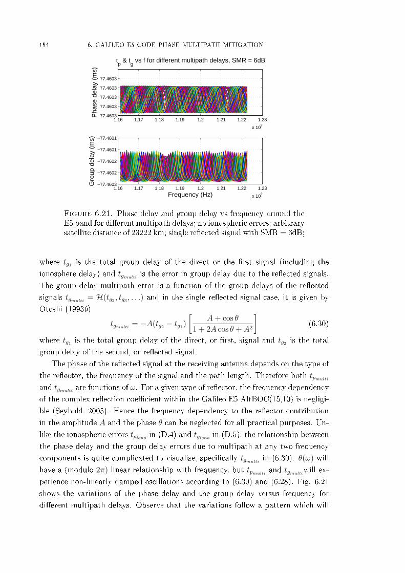
154 6. GALILEO E5 CODE PHASE MULTIPATH MITIGATION
1.16 1.17 1.18 1.19 1.2 1.21 1.22 1.23
x 109
77.4603
77.4603
77.4603
77.4603
77.4603
Pha
se d
elay
(m
s)
tp & t
g vs f for different multipath delays, SMR = 6dB
1.16 1.17 1.18 1.19 1.2 1.21 1.22 1.23
x 109
−77.4603
−77.4602
−77.4602
−77.4601
−77.4601
Gro
up d
elay
(m
s)
Frequency (Hz)
Figure 6.21. Phase delay and group delay vs frequency around theE5 band for di�erent multipath delays; no ionospheric errors; arbitrarysatellite distance of 23222 km; single re�ected signal with SMR = 6dB;
where tg1 is the total group delay of the direct or the �rst signal (including the
ionosphere delay) and tgmulti is the error in group delay due to the re�ected signals.
The group delay multipath error is a function of the group delays of the re�ected
signals tgmulti = H(tg2 , tg3 , . . .) and in the single re�ected signal case, it is given by
Otoshi (1993b)
tgmulti = −A(tg2 − tg1)[
A+ cos θ
1 + 2A cos θ + A2
](6.30)
where tg1 is the total group delay of the direct, or �rst, signal and tg2 is the total
group delay of the second, or re�ected signal.
The phase of the re�ected signal at the receiving antenna depends on the type of
the re�ector, the frequency of the signal and the path length. Therefore both tpmultiand tgmulti are functions of ω. For a given type of re�ector, the frequency dependency
of the complex re�ection coe�cient within the Galileo E5 AltBOC(15,10) is negligi-
ble (Seybold, 2005). Hence the frequency dependency to the re�ector contribution
in the amplitude A and the phase θ can be neglected for all practical purposes. Un-
like the ionospheric errors tpiono in (D.4) and tgiono in (D.5), the relationship between
the phase delay and the group delay errors due to multipath at any two frequency
components is quite complicated to visualise, speci�cally tgmulti in (6.30). θ(ω) will
have a (modulo 2π) linear relationship with frequency, but tpmulti and tgmultiwill ex-
perience non-linearly damped oscillations according to (6.30) and (6.28). Fig. 6.21
shows the variations of the phase delay and the group delay versus frequency for
di�erent multipath delays. Observe that the variations follow a pattern which will

6.5. A GROUP DELAY COMPENSATION VIEWPOINT FOR THE SCPC METHOD 155
be further explored later in this chapter.
Relation between the phase/group delay and the phase measurement
errors in GNSS. From (D.4) and (6.28) it can be inferred that the phase delay
results in carrier phase measurement error. The relation is straightforward; if the
phase delay is tp, then the carrier phase measurement will incur a phase error of
the same amount. On the other hand, the relationship between the group delay in
(D.5) and (6.30), and the code phase measurement error is not easy to visualise.
The optimal tracking circuitry for synchronising the spreading code involves a delay
locked loop Parkinson and Spilker (1995). In an attempt to measure the group
delay in spread spectrum systems, Otoshi (1993a) shows that the timing error of an
early/late code correlator indicates the group delay experienced by the signal and
is explored further in the following sub sections for the AltBOC(15,10) signal.
6.5.1. The received signal and the tracking architecture. The received
signal along with N − 1 re�ected signals can be expressed as
r(t) = <{P0 · s(t− tgiono − tgoth) · exp (jωeff (t+ tpiono + tpoth)) +
N−1∑i=1
Pi · s(t− tgiono − tgimulti − tgoth) · exp (jωeff (t+ tpiono + tpimulti + tpoth))} (6.31)
where tpoth and tgoth represent the phase delay and group delay respectively, due
to all other sources than the ionosphere and the multipath, P denotes the received
signal power, ωeff denotes the e�ective frequency (including Doppler). These sources
mainly include the signal transit time, the troposphere error, antenna-induced errors,
and the errors in the receiver due to the RF down converter and �lter(s). Depending
on the method of down conversion, r(t) could be either complex or real. However,
bandpass sampling to a moderate IF is assumed in this work and as a result r(t) is
real.
The tracking architecture used in the following sections is the architecture used
for the SCPC method as shown in Fig. 6.11. Note that the code phase estimates
of the wideband E5 AltBOC(15,10) tracking are provided to the code generation
modules of the sideband tracking.
6.5.2. Mitigating the ionospheric and multipath errors.
6.5.2.1. Mitigating the e�ects of ionosphere (in the absence of multipath errors).
One of the main features of Galileo E5 AltBOC modulation is that the E5a and
E5b sidebands can be processed independently of each other. Hence it is possible to
obtain three code and carrier phase measurements from E5a , E5b and the wideband
E5 that can be used to obtain estimates of ionosphere-induced errors.

156 6. GALILEO E5 CODE PHASE MULTIPATH MITIGATION
0 10 20 30 40 50 60 70 80 90 100−1
−0.5
0
0.5
1x 10
−8
∆ t p(s)
0 10 20 30 40 50 60 70 80 90 100−4
−3
−2
−1
0x 10
−10
∇∆t p(s
)
Ionospheric error at E5 (m)
E5−E5aE5−E5b
∆tpE5−E5a
− ∆tpE5−E5b
Figure 6.22. Di�erence in the phase delays in E5a and E5b withrespect to E5 (top); di�erence of the two curves in the top �gure(bottom)
Figures 6.22 and 6.23 show the di�erence in the phase delay and the correlation
values (note the di�erence in scales). The corresponding parameters at the centre
frequency are used as references to obtain the di�erences. An interesting point to
note is that within the E5 band, due to the near-symmetric nature of the ionospheric
group delay dispersion, the code phase estimates from the E5a and E5b tracking
loops are a�ected in an opposite manner when referred to the code phase estimates
of the wideband E5 signal tracking loop. Observe that the di�erence between E5-E5a
and E5-E5b is only up to 0.33 ns (0.33 ns is for a very high ionospheric delay of 100
m) which shows that one can use the combination of E5a and E5b measurements to
obtain a good estimate of the ionospheric delay at the centre frequency. Nevertheless,
the quality of such estimate depends on the contribution of the receiver noise.
6.5.2.2. Mitigating the e�ects of multipath (in the absence of ionospheric errors).
The e�ect of the phase delay and the group delay for di�erent multipath delays and
di�erent frequency components around the E5 band was shown in the previous
section. It is important to observe the behaviour of the phase and group delays at
the E5a, E5b and E5 centre frequencies. Fig. 6.24 shows the di�erence of phase
delay and group delay between E5a and E5b frequencies. This plot is generated
using (6.28) and (6.30). It should be noted that the equation only involves the
carrier frequencies and does not include the e�ects of the spreading code.
With the spreading code in place, the errors at larger multipath delays are at-
tenuated, following the shape of the correlation function. The composite phase
delay and the composite group delay for a single re�ection case at the output of the

6.5. A GROUP DELAY COMPENSATION VIEWPOINT FOR THE SCPC METHOD 157
0 10 20 30 40 50 60 70 80 90 1000
0.2
0.4
0.6
0.8
1
Cor
rela
tion
loss
(dB
)
0 10 20 30 40 50 60 70 80 90 1000
0.01
0.02
0.03
0.04∆
corr
elat
ion
loss
es (
dB)
Ionospheric error at E5 (m)
E5aE5b
E5a − E5b
Figure 6.23. Di�erence in the correlation values in E5a and E5bsignal components with respect to Ionosphere free situation (top);di�erence of the two curves in the top �gure (bottom)
0 5 10 15 20 25 30−2
−1
0
1
2x 10
−10
t p E5b
−t p E
5a
(s)
0 5 10 15 20 25 30−2
−1
0
1
2x 10
−7
t g E5b
−t g E
5a
(s)
Multipath delay (m)
Figure 6.24. Di�erence of E5a and E5b phase and group delaysfor di�erent multipath delays (analytical); single re�ected signal case;A=0.5;
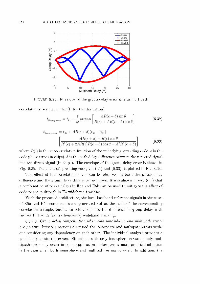
158 6. GALILEO E5 CODE PHASE MULTIPATH MITIGATION
0 5 10 15 20 25 30−6
−4
−2
0
2
4
6
Multipath Delay (m)
Gro
up D
elay
(m
)
E5 LBE5 UBE5a UBE5a LB
Figure 6.25. Envelope of the group delay error due to multipath
correlator is (see Appendix (I) for the derivation):
tpcomposite = tp1 −1
ωarctan
[AR(ε+ δ) sin θ
R(ε) + AR(ε+ δ) cos θ
](6.32)
tgcomposite = tg1 + AR(ε+ δ)(tg2 − tg1)[AR(ε+ δ) +R(ε) cos θ
R2(ε) + 2AR(ε)R(ε+ δ) cos θ + A2R2(ε+ δ)
](6.33)
where R(.) is the autocorrelation function of the underlying spreading code, ε is the
code phase error (in chips), δ is the path delay di�erence between the re�ected signal
and the direct signal (in chips). The envelope of the group delay error is shown in
Fig. 6.25. The e�ect of spreading code, via (I.1) and (6.33), is plotted in Fig. 6.26.
The e�ect of the correlation shape can be observed in both the phase delay
di�erence and the group delay di�erence responses. It was shown in sec. (6.3) that
a combination of phase delays in E5a and E5b can be used to mitigate the e�ect of
code phase multipath in E5 wideband tracking.
With the proposed architecture, the local baseband reference signals in the cases
of E5a and E5b components are generated not at the peak of the corresponding
correlation triangle, but at an o�set equal to the di�erence in group delay with
respect to the E5 (centre frequency) wideband tracking.
6.5.2.3. Group delay compensation when both ionospheric and multipath errors
are present. Previous sections discussed the ionosphere and multipath errors with-
out considering any dependency on each other. The individual analysis provides a
good insight into the errors. Situations with only ionosphere errors or only mul-
tipath error may occur in some applications. However, a more practical situation
is the case when both ionosphere and multipath errors co-exist. In addition, the

6.5. A GROUP DELAY COMPENSATION VIEWPOINT FOR THE SCPC METHOD 159
0 5 10 15 20 25 30−2
−1
0
1
2x 10
−10
t p E5b
−t p E
5a
(s)
0 5 10 15 20 25 30−2
−1
0
1
2x 10
−7t g E
5b
−t g E
5a
(s)
Multipath delay (m)
Without the spreading codeWith the spreading code
Without the spreading codeWith the spreading code
Figure 6.26. Di�erence of E5a and E5b phase and group delays fordi�erent multipath delays (analytical); single re�ected signal; A=0.5
receiver may experience range estimation errors from sources such as troposphere
errors, estimation of the clock error (both satellite and the receiver), satellite posi-
tion and velocity estimation (due to orbit parameters / ephemeris), previous epoch
pseudorange estimation error and other secondary e�ects. It is assumed in this work
that all errors from the other sources are frequency independent.
Fig. 6.27 shows the phase delay and group delay for E5a, E5b and E5 frequencies
vs. multipath delay for three ionospheric delays, viz. 0m, 50m and 100m, experi-
enced at the centre frequency. The error shape due to the multipath is not visible
because the magnitude of the multipath error is small compared to the scale of the
plots.
Fig. 6.28 shows the phase delay and group delay di�erences at di�erent iono-
spheric delays and multipath delays. Observe that the di�erence in phase delay
shows an o�set depending on the ionospheric delay. The error due to multipath
is around this o�set. The group delay di�erence also shows a similar behaviour.
However, the error due to multipath is of an order comparable to the ionosphere
errors for the delays shown in Fig. 6.28. The phase delay di�erences
tpbc = tpE5b− tpE5
tpca = tpE5− tpE5a
tpba = tpE5b− tpE5a
(6.34)
provide an easy computation of the ionosphere-a�ected phase at the E5 centre fre-
quency due to the similar di�erences with respect to both the side bands. This
is expected as the ionospheric delay is almost symmetrical around the E5 centre

160 6. GALILEO E5 CODE PHASE MULTIPATH MITIGATION
0 5 10 15 20 25 30−4
−2
0
2
4
t p (ra
d)
0 5 10 15 20 25 304708
4709
4710
4711
4712
4713
t g (ch
ips)
Multipath delay (m)
E5a, 0mE5a, 50mE5a, 100mE5b, 0mE5b, 50mE5b, 100mE5, 0mE5, 50mE5, 100m
Figure 6.27. Phase delay and group delay for E5a, E5b and E5frequencies under multipath condition for di�erent ionospheric delay;nominal satellite distance of 23222km; single re�ected signal; A=0.5
frequency. It should be noted that the knowledge of integer number of cycles is not
required for two reasons:
(1) Because the phase di�erence method experiences the oscillations at the
frequency di�erence (30.690 MHz for E5b-E5a and 15.345 MHz for E5b-
E5c or E5b-E5) there can be a maximum of 3 cycles di�erence between E5a
and E5b for ionospheric delays of up to 100 m (1.5 cycles in the other two
cases).
(2) The availability of three phase measurements helps isolate the ionosphere
error at the centre frequency.
To mitigate the e�ects of multipath the, SCPC method discussed in sec. (6.3) is
used here. Referring back to Fig. 6.28, a two-step approach is followed here, �rst to
resolve the ionospheric error and second to apply the SCPC algorithm to mitigate
the multipath error. The di�erence in the phase delays of the E5a and E5b signal
component tracking is nothing but the slope of the phase response over the entire
band and hence represents the group delay at the centre frequency E5=1191.795
MHz.
E�ect of previous epoch pseudorange errors on the ionosphere and
multipath mitigation process. As mentioned earlier, apart from the two major
errors under consideration, the receiver may experience other frequency-independent
errors. As an example assume that the pseudorange is in error. The �rst consequence
of this erroneous pseudorange is that the phase and the chip shift (fractional) of the
incoming signal di�er from the actual values. However, this error will be common

6.5. A GROUP DELAY COMPENSATION VIEWPOINT FOR THE SCPC METHOD 161
0 5 10 15 20 25 30−3
−2
−1
0
1
2
t p diff
(ra
d)
0 5 10 15 20 25 30−0.4
−0.2
0
0.2
0.4
t g diff
(ch
ips)
Multipath delay (m)
E5b−E5a, 0mE5b−E5a, 50mE5b−E5a, 100mE5b−E5, 0mE5b−E5, 50mE5b−E5, 100mE5−E5a, 0mE5−E5a, 50mE5−E5a, 100m
Figure 6.28. Phase delay and group delay di�erences at di�erentionospheric delays and multipath delays
to all three components E5, E5a and E5b of the signal and the method of obtaining
the di�erence in phase delay and the di�erence in group delays nulli�es this common
error. The second consequence is the e�ect of this pseudorange error on the code
multipath error. In (I.1) and (6.33), the ε parameter which indicates the error in the
pseudorange alters the multipath error characteristics. Thanks to the SCPC method
the code delay estimates from the E5 AltBOC(15,10) tracking loop are provided to
the code delay estimates of the two sidebands. With this sort of aiding, all the three
components of the signal calculate the pseudorange estimates from a single source
(of the previous instant) and keep the noise characteristics undisturbed. Hence the
e�ect of pseudorange error on the multipath error is removed by the tracking loop
architecture.
E�ect of Doppler frequency on the ionosphere and multipath miti-
gation process. In moderate to high dynamics applications, each frequency com-
ponent of the wideband signal experiences di�erent Doppler shifts. In the case of
Galileo E5 AltBOC(15,10), the Doppler frequencies observed on the E5a and E5b
components di�er from those of the wideband AltBOC tracking that experiences a
Doppler corresponding to the centre frequency E5. However, aiding the E5a and
E5b carrier tracking loops with the frequency estimate of the E5 AltBOC tracking
loop eliminates the e�ect of any di�erence in Doppler frequency estimation in the
sideband tracking loops. Second, the e�ect of the rate of change of the user dynam-
ics on the multipath is discussed in Nedic (2009). In the case of E5a and E5b, these
errors will be opposing each other when referenced to the E5 centre frequency. Hence
the di�erence of E5a and E5b carrier phase measurements is devoid of range-rate
e�ects.

162 6. GALILEO E5 CODE PHASE MULTIPATH MITIGATION
E�ect of antenna induced errors on the ionosphere and multipath miti-
gation process. Due to practical limitations in the antenna design, some properties
of the antenna depend on the frequency (Orban and Moernaut, 2009). Of interest
to this chapter are the phase centre and the axial ratio. The phase centre of the
antenna varies with frequency and boresight angle. The axial ratio of the antenna
which is an indicator of the amount of the rejection of a LHCP (re�ected) signal
varies with the frequency and the incidence angle (Yun et al., 2008; Zhuang and
Tranquilla, 1995). Knowing the frequency dependent variation will help in calibrat-
ing for that e�ect. However, the variation caused by the incidence angle cannot be
calibrated a priori because the angle of incidence of the re�ected signal will not
be known. A possible solution is to employ multiple closely spaced antennas (Ray,
2000). A detailed analysis of the antenna-induced errors is beyond the scope of this
thesis.
6.5.3. Simulation results and discussion. To test the multipath mitigation
technique in the presence of ionosphere, the GIOVE-A E5 AltBOC(15,10) signal
structure is used as a reference. Two types of veri�cation of the technique mentioned
in the previous section are performed. In the �rst case, the signal with the multipath
and the ionosphere e�ects is generated in a Matlab environment. In the second, an IF
signal is collected from the GIOVE-A satellite, ensuring that there are no re�ectors
within a distance of 30 metres that can cause multipath errors. Then, ionosphere
and multipath errors are added using Matlab (at the IF stage) to this signal. This
signal is termed a �pseudo-real� signal. The IF samples of the GIOVE-A satellite
signal were collected using the Septentrio GeNeRx1 receiver which has the capability
to output 150 ms of IF signal sampled at 112 MHz. The bandwidth of the receiver
is 55 MHz around the E5 centre frequency. The simulated delay distortions are
added to the signal from the 60th ms. Figs. 6.29 and 6.30 show the results of the
SCPC method with simulated ionosphere errors.Fig. 6.29 shows the performance
of the group delay compensation technique at a particular multipath delay for two
ionospheric delay errors of 50 m and 100 m. Again, the reduction in the code phase
error is clear from the simulated signal. With the real signal the error itself is small,
as shown in the top left portion of Fig. 6.30. However, the group delay compensation
brings down a signi�cant part of this error.
6.6. Summary
In this chapter, a code phase multipath mitigation method called SCPC (Side-
band Carrier Phase Combination) was presented. The SCPC method makes use of
the carrier phases of E5a and E5b sidebands to estimate the code phase multipath
at the centre of the E5 band that is experienced by a Direct AltBOC tracking. An

6.6. SUMMARY 163
0 50 100−0.04
−0.03
−0.02
−0.01
0
0.01
0.02Code phase
0 50 100−10
−8
−6
−4
−2
0
2
4x 10
−3 Difference in cp
0 20 40 60 80 100 120 140−0.01
−0.005
0
0.005
0.01
0.015Code minus scaled cp diff
Time (ms)
50m iono100m iono
Figure 6.29. Multipath mitigation with the simulated signal withmultipath at 5.4m and ionospheric delays of 50m and 100m at E5
0 50 100 150−0.2
0
0.2
0.4
0.6Code phase (chips)
0 50 100 150−0.3
−0.2
−0.1
0
0.1
0.2Code minus scaled cp diff
Time (ms)
0 50 100 150−0.15
−0.1
−0.05
0
0.05Difference in carrier phases
50m100m
Figure 6.30. Multipath mitigation with the pseudo-real signal withmultipath at 5.4m and ionospheric delays of 50m and 100m at E5

164 6. GALILEO E5 CODE PHASE MULTIPATH MITIGATION
architecture to realise the SCPC method was described. The applicability of the
SCPC method was discussed and the results obtained with real satellite signal tests
were presented. It is shown that the method can reduce the code multipath error
to less than 0.5 metres for the E5 AltBOC.
The proposed SCPC technique compensates for the propagation delay distortion
without the need of estimating the absolute value of either the ionospheric or multi-
path delay. In summary, the proposed group delay compensation technique exploits
the multi-frequency, wideband feature of the AltBOC modulation to generate an
accurate range measurement.

CHAPTER 7
Galileo E5 Baseband Hardware
7.1. Introduction
This chapter mainly deals with two aspects of the Galileo E5 baseband hardware.
The �rst part addresses the problem of e�ciently computing the FFTs required
to acquire signals of varying code lengths. The requirements of FFT-based algo-
rithms for a multi-band receiver are discussed and the application of prime-factor
and mixed-radix FFT algorithms is analysed. A novel way of factorising di�erent
transform lengths into smaller transforms and then combining these smaller-point
FFTs to compute the larger required FFTs is described.
The second part of this chapter describes an e�cient way of realising the core cor-
relator functionality for the E5 signal, estimates the hardware resource requirement
and power consumption, and compares it with other signals.
Sec. 7.2 to sec. 7.7 of this chapter contain work published in Journal of GPS,
2009 (Shivaramaiah et al., 2009b), while sec. 7.8 contains the work published in
ISCAS 2010 (Shivaramaiah and Dempster, 2010b).
The chapter is organised as follows. Sec. 7.2 describes the receiver model and
search dimensions in the context of a multi-band GNSS receiver, sec. 7.3 describes
the FFT requirements of new GNSS signals, and sec. 7.4 describes the proposed
mixed-radix approach along with the result of transform length factorisation for the
di�erent signal types. Sec. 7.5 discusses computational complexity by comparing
the standard and proposed approaches. Sec. 7.6 describes the FPGA resource
utilisation of the proposed methods, followed by a comparison for some of the signal
combinations in sec. 7.7. Sec. 7.8 compares the resource utilisation and power
consumption of the core correlator used for signal tracking.
7.2. GNSS Receiver Model and Search Dimensions
7.2.1. The receiver model. The received signal in a multi-band GNSS re-
ceiver capable of receiving the open access signals (or components of these signals)
GPS L1 C/A, L2 and L5, Galileo E1 and E5 is down converted, sampled and digi-
tised to obtain an Intermediate Frequency (IF) equivalent. Assuming separate down
conversion paths for the L1, L2 and L5 bands, the received signal is transformed
165

166 7. GALILEO E5 BASEBAND HARDWARE
RF front-end
Digitized IF samples
Clock Source
Carrier Removal
Code Correlation Controller
Antenna
Commands
Decision
Correlation Values
Correlator
r(t) r1(n)
r2(n)
r5(n)
Figure 7.1. Block diagram of a multi-band receiver
into three equivalent IF signals:
r(t)down-conversion
=⇒ r1(t) + r2(t) + r5(t) (7.1)
with the individual signals being (for one satellite from each system)
r1(t) = AL1sL1(t− τL1) cos ((ωIF1 + ωdL1) t+ θL1)
+AE1sE1(t− τE1) cos ((ωIF1 + ωdE1) t+ θE1) (7.2)
r2(t) = AL2sL2(t− τL2) cos ((ωIF2 + ωdL2) t+ θL2) (7.2a)
r5(t) = AL5sL5(t− τL5) exp {j [(ωIF5 + ωdL5) t+ θL5]}
+AE5sE5(t− τE5) exp {j [(ωIF5 + ωdE5) t+ θE5]} (7.2b)
where AX is the amplitude, sX is the modulating baseband component, τX is the
delay and θX is the phase of the signal X, and ωIF1 ,ωIF2 ,wIF5 are the intermediate
frequencies. As the �rst stage within the receiver the nominal carrier frequency is
removed. The output of this carrier removal process then comprises only the base-
band component of the received signal plus any Doppler. It is this baseband version
that is considered for the proposed code acquisition approach in the discussions
throughout the remainder part of this chapter. Fig. 7.1 illustrates such a receiver.
Because of their signal structure, each of these signals has a di�erent requirement of
the minimum sampling frequency. As will be explained later, the minimum number
of cells to search within the code acquisition block depends on the length of the
spreading code and the modulation rather than on the sampling frequency. Note
that only the baseband signal is of interest and the RF down converter and antenna
are beyond the scope of this discussion. In addition, depending on the design, the
receiver may process any combination of the above signals.
7.2.2. Search dimensions for signal acquisition in a multi-band GNSS
receiver. In this section new parameters associated with the concept of search
engine dimensions are introduced. Acquisition has been discussed in the literature
as a two-dimensional search (Kaplan and Hegarty, 2006) when the receiver knows

7.2. GNSS RECEIVER MODEL AND SEARCH DIMENSIONS 167
PRN Code Number
Code Delay
Doppler Frequency
Code Length
Signal TypePRN Code Number
Doppler Frequency
(a) (b)
Figure 7.2. Search dimensions in a (a) single-band GNSS receiveremploying the time domain correlation approach (b) multi-band GNSSreceiver employing the FFT-based code acquisition approach
the PRN code which it is searching for, or as a three-dimensional search otherwise
(Djebouri et al., 2006). When the acquisition process is considered as a whole
(search engine plus the controller) instead of just the search engine, the search is
three-dimensional. The parameter along the code dimension in a GNSS receiver
employing a time domain correlation approach for acquisition is the code delay (see
Fig. 7.2a). In a single-band receiver employing an FFT-based acquisition approach
there is no parameter along the code dimension as the search is performed over the
entire code space at once. The size of the FFT block depends on the code length
and the desired resolution of the code search. However in a multi-band receiver the
code length is still a varying parameter and this is used along the code dimension.
With the new GNSS signals in context, because of the varying code length and
varying search step requirements, the acquisition engine needs to be re-arranged
whenever the same hardware resource needs to be used across di�erent signals.
Hence this parameter introduces another dimension in the search process which is
referred to here as the `signal' dimension. Fig. 7.2b depicts the four dimensions in
the context of a multi-band GNSS receiver. Note that the variables in each dimension
are not totally independent. For example the same PRN may have di�erent code
delay search requirements depending on the signal type.
During the signal acquisition process, the selection of the resolution of the coarse
estimates of chip delay and Doppler frequency depends on the requirements of the
succeeding tracking stage - typical values for GPS L1 C/A being 0.5 chips for the
code delay and 500 Hz (for one millisecond coherent integration) for the Doppler
frequency. The number of time cells to search depends on the code length. The
number of frequency cells to search depends on the total frequency ambiguity and
also on the coherent integration time. As an example, for an L5 code length of
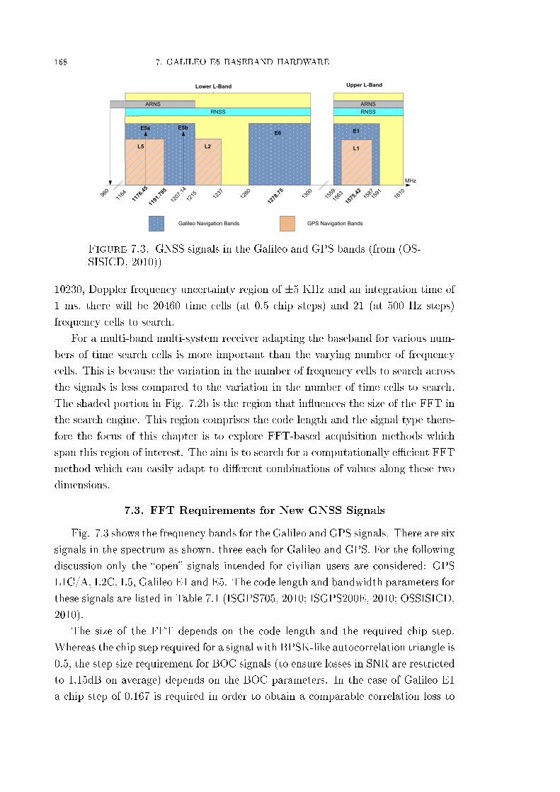
168 7. GALILEO E5 BASEBAND HARDWARE
ARNSRNSS
ARNSRNSS
960
1164
1176
.45
1191
.795
1207
.14
1215 12
3712
60
1278
.75 1300
156315
59
1575
.42 1587
1591
1610
Lower L-Band Upper L-Band
E5a E5b
L5 L2 L1
E6 E1
Galileo Navigation Bands GPS Navigation Bands
MHz
Figure 7.3. GNSS signals in the Galileo and GPS bands (from (OS-SISICD, 2010))
10230, Doppler frequency uncertainty region of ±5 KHz and an integration time of
1 ms, there will be 20460 time cells (at 0.5 chip steps) and 21 (at 500 Hz steps)
frequency cells to search.
For a multi-band multi-system receiver adapting the baseband for various num-
bers of time search cells is more important than the varying number of frequency
cells. This is because the variation in the number of frequency cells to search across
the signals is less compared to the variation in the number of time cells to search.
The shaded portion in Fig. 7.2b is the region that in�uences the size of the FFT in
the search engine. This region comprises the code length and the signal type there-
fore the focus of this chapter is to explore FFT-based acquisition methods which
span this region of interest. The aim is to search for a computationally e�cient FFT
method which can easily adapt to di�erent combinations of values along these two
dimensions.
7.3. FFT Requirements for New GNSS Signals
Fig. 7.3 shows the frequency bands for the Galileo and GPS signals. There are six
signals in the spectrum as shown, three each for Galileo and GPS. For the following
discussion only the �open� signals intended for civilian users are considered: GPS
L1C/A, L2C, L5, Galileo E1 and E5. The code length and bandwidth parameters for
these signals are listed in Table 7.1 (ISGPS705, 2010; ISGPS200E, 2010; OSSISICD,
2010).
The size of the FFT depends on the code length and the required chip step.
Whereas the chip step required for a signal with BPSK-like autocorrelation triangle is
0.5, the step size requirement for BOC signals (to ensure losses in SNR are restricted
to 1.15dB on average) depends on the BOC parameters. In the case of Galileo E1
a chip step of 0.167 is required in order to obtain a comparable correlation loss to

7.3. FFT REQUIREMENTS FOR NEW GNSS SIGNALS 169
Table 7.1. GPS and Galileo signal parameters of interest
Signal Name Code Length Chipping
Rate (MHz)
Receiver
Bandwidth
in MHz
(typical)
GPS L1 C/A 1023 1.023 2
GPS L2C-CM 20460 0.5115 2
GPS L2C-CL* 767250 0.5115 2
GPS L5 10230 10.23 20
Galileo E1B/ E1C 4092 1.023 4
Galileo E5 10230 10.23 50
Galileo E5a /E5b 10230 10.23 20
*L2C-CL is generally not targetted in the �rst stage of acquisition (Dempster, 2006) and
hence not included in the discussions in this chapter.
Table 7.2. Transform length requirements Case 1 � 0.5 chip step
Signal Name Chip StepSize
RequiredTransform Length
GPS L1 C/A 0.5 2046Galileo E1B/C� SA 0.5(Side-band
Acquisition)8184
GPS L2C 0.5 40920GPS L5 0.5 20460
Galileo E5a/E5b 0.5 20460
that for the BPSK 0.5 chip step (De Wilde et al., 2006). Hence for the Galileo
E1B/C signal, the number of time cells to search increases from 8184 to 24552
for one millisecond coherent integration duration, despite the signal bandwidth only
doubling. For the analysis of the FFT requirements and of the proposed approaches,
a coherent integration time of one primary code period is considered in this chapter.
As already mentioned, the transform length can be reduced to as much as twice
the code length for some of the signals. This is true for the GPS L1, L2, L5, Galileo
E5a and E5b signals where the shape of the autocorrelation function allows half chip
(or less) alignment between the received and local signals with an e�ective sample
size of twice the code length. For these signals the transform length requirements
are given in Table 7.2 (Case 1).
For the Galileo E1B/C and E5 signals, the e�ective sample sizes for one millisec-
ond, which is the transform length, are shown in Table 7.3 (Case 2). Note that for
the Galileo E1B/C, the signal can be acquired with 0.5 chip spacing with the Side-
band Acquisition (SA) method (but with 3dB correlation loss compared to BPSK
0.5 chip spacing), or the Direct Acquisition (DA) method with a 0.167 chip spacing

170 7. GALILEO E5 BASEBAND HARDWARE
Table 7.3. Transform length requirements Case 2 � other chip steps
Signal Name Chip Step Size RequiredTransform Length
Galileo E1B/C� DA 0.167(Direct Acquisition) 24552Galileo E5a/E5b 0.083 122760
Table 7.4. Transform length requirement summary
Signal Name Required Transform Length
GPS L1 C/A 2046Galileo E1B/C� SA 8184
GPS L5, Galileo E5a/E5b 20460Galileo E1B/C � DA 24552
GPS L2C 40920Galileo E5a/E5b 122760
(no loss compared to BPSK 0.5 chip spacing).
It is clear from the discussions so far that there is a common transform length
requirement among the signals. Table 7.4 combines all the signals with respect
to the transform length and summarises the requirements for the signals under
consideration. The chip step size for each signal is the same as in Tables 7.2 and
7.3.
A typical implementation of FFT-based acquisition has two problems. The �rst
problem is due to the transform length. In order to simplify the FFT implementa-
tion, often a �next immediate of power-of-two� transform length is chosen instead
of the transform lengths listed in Table 7.4, by zero-padding the input sequence.
Even though this works well for the GPS L1 signal (1024 instead of 1023), for the
codes with longer lengths one might have to unnecessarily increase the transform
length by a signi�cant amount (e.g. 65536 instead of 40920 for the GPS L2C) which
also may reduce the SNR of the correlation output (Yang 2001). It should be noted
that there are di�erent contexts where the method of zero-padding is used. Yang
(2001) describes the method of zero-padding to perform circular correlation and
linear correlations at arbitrary lengths. On the other hand Dempster (2006) de-
scribes a method of zero-padding for the L2C signal acquisition. In the discussions
this zero-padding is considered as a consequence of making the transform length a
power-of-two (including any acquisition concept related zero-padding as in the case
of L2C). The second problem is the fact that di�erent signals require FFT blocks
of di�erent sizes. For example, assuming one millisecond coherent integration, a
receiver processing GPS L1 C/A and Galileo E1B/C will have to have both 2046
point, as well as 8184 point FFTs (in the case of the SA method for E1). This
results in allocating dedicated FFT blocks for each signal, which is a very expensive

7.4. THE PROPOSED FFT BASED CODE CORRELATION APPROACH 171
Table 7.5. 1023 point FFT factorisation
Transform length Factors
1023 3, 11, 31
Table 7.6. Transform length factorisation
Signal Name Transform Length Factors
GPS L1 C/A 2046 2, 1023Galileo E1B/C� SA 8184 8, 1023
GPS L5, Galileo E5a/E5b 20460 4, 5, 1023Galileo E1B/C � DA 24552 3, 8, 1023
GPS L2C 40920 5, 8, 1023Galileo E5a/E5b 122760 3, 5, 8, 1023
approach.
7.4. The Proposed FFT Based Code Correlation Approach
In this section, �rst the rationale behind the factorisation of large-point FFTs
is described. Next, the computational complexity of the small-point FFT blocks is
discussed and it is shown that a small modi�cation to the �brute-force� factorisa-
tion method can result in the e�cient computation of the small-point FFT blocks.
Finally, with the revised factorisation, a table of required small-point FFT blocks is
given.
7.4.1. Factoring of FFT transform lengths. The basic idea is to factor N
(for an N -Point FFT) into two or more smaller integers, implement the small-point
building blocks, and combine them to obtain the �nal result. Thus for the two-factor
case, i.e., if N can be factored into N = P · Q then, Q number of P -point FFTs
and P number of Q-point FFTs are combined to form the N -point FFT. Appendix
C describes two methods of factoring the FFT transform lengths, the prime-factor
method and the mixed-radix method.
All the transform length requirements listed in Table 7.4 are multiples of 1023.
It should be noted that 1023 is easily factored into three prime numbers: 3, 11 and
31 (Table 7.5). All other transform lengths can be factorised such that the factors
are relatively prime to 1023. This factorisation is shown in Table 7.6. It can be
seen that the transform of length 1023 is common across all the transform lengths,
hence it makes sense to have the 1023-point FFT as a single block, which can be
implemented using the prime-factor approach. The basic small-point building blocks
required for all transform lengths under consideration are listed in Table 7.7. This
list assumes a 1023-point block as a single entity (as mentioned above).

172 7. GALILEO E5 BASEBAND HARDWARE
Table 7.7. FFT blocks required for GNSS signals in consideration
Basic Building Blocks
2, 3, 4, 5, 8, 11, 31, 1023
Table 7.8. Complexity of small-point blocks
Transform Length Additions Multiplications
2 4 03 12 44 16 05 34 108 52 411 168 4016 148 2031 776 160
7.4.2. Complexity of small-point blocks. Many algorithms are available
for computing the small-point FFTs, such as the Winograd, Rader, SWIFT, Prime-
length, etc (Smith, 1995). Each algorithm has its own complexity (number of ad-
ditions and multiplications). For the sake of commonality amongst di�erent combi-
nations of small-point blocks, Table 7.8 lists the number of real additions and mul-
tiplications that are required (Smith, 1995; Burrus and Selesnick, 1995). Note that
if there exists a method which can more e�ciently compute the small-point FFTs,
the improvement is directly observed in the proposed prime-factor and mixed-radix
approaches as well because the proposed method uses a combination of the basic
small-point blocks.
7.4.3. A note on 1023-point and 1024-point FFTs. As mentioned previ-
ously, 1023 is a common factor in the transform lengths of all the signals under
consideration. But because 1024 is the next immediate power-of-two number for
1023 it can be implemented using Radix-2, Radix-4 or other optimised algorithms.
Therefore it is necessary to compare the performance of the prime-factor approach
for a 1023-point FFT with a 1024-point FFT (with padding of one zero). It was
shown in Proakis and Manolakis (1995) that the Split-radix FFT algorithm requires
fewer multiplications and additions compared to the Radix-2 and Radix-4 algo-
rithms. Split-radix is a method in which at each stage the transform is divided into
Radix-2 and Radix-4 branches (not FFTs) and then blended in the next stage. It
should not be confused with the Mixed-radix which uses the factors (i.e. the smaller
FFTs) of the transform length at each stage. Table 7.9 lists the operation count
comparison for the 1023-point FFT using the prime-factor approach and the 1024-
point FFT using the Radix-2, Radix-4 and Split-radix approaches. Note that the

7.5. COMPUTATIONAL COMPLEXITY OF THE PROPOSED APPROACH 173
Table 7.9. Operation count for 1023 and 1024 point FFTs
Transform Length Algorithm Additions Multiplications
1023 Prime-factor 45324 103641024 Radix-2 46080 153601024 Radix-4 49920 115201024 Split-radix 27652 7172
Table 7.10. Revised transform lengths for di�erent signals
Signal Name Required Transform Length Factors
GPS L1 C/A 2048 2, 1024Galileo E1B/C� SA 8192 8, 1024
GPS L5, Galileo E5a/E5b 20480 4, 5, 1024Galileo E1B/C � DA 24576 3, 8, 1024
GPS L2C 40960 5, 8, 1024Galileo E5 122880 3, 5, 8, 1024
Table 7.11. FFT blocks required for GNSS signals in consideration� revised
Basic Building Blocks
2, 3, 4, 5, 8, 1024
Split-radix approach is the �cheapest� of all the considered approaches for the 1023
or 1024-point FFT. With this information it is therefore wise to choose 1024 as the
common factor instead of 1023.
7.4.4. Revised FFT transform lengths and their factors. The revised
transform length requirements are given in Table 7.10. The revised requirements of
the basic building blocks are given in Table 7.11. Since the factors are not relatively
prime, the method to be used to combine the small-point blocks is the Mixed-radix
method.
7.5. Computational Complexity of the Proposed Approach
In order to compare the complexity of the proposed approaches, the Split-radix
algorithms for the power-of-two approaches with the number of real additions and
real multiplications according to Sorensen et al. (1986) (the complex multiplications
are treated as 3 real multiplications and 3 real additions) are used. Table 7.12 gives a
comparison of the Split-radix approach and the Mixed-radix approach. To compute
the number of operations for the Mixed-radix algorithms, the factorisation according
to Tables 7.10 and 7.4 has been used. As an example, consider the transform length
2048 for which 2-point and 1024-point FFT blocks are needed. In the �rst stage,
all the 1024 two-point FFTs are computed. The outputs of these FFTs are then

174 7. GALILEO E5 BASEBAND HARDWARE
Table 7.12. Computational complexity comparison
Split Radix Mixed Radix
Transform
Length
Additions Multipli-
cations
Transform
Length
Additions Multipli-
cations
2048 61444 16388 2048 62649 17413
4096 135172 36868 4096 136199 37895
8192 294916 81924 8192 295947 82955
16384 638980 180228 16384 640019 181267
32768 1376260 393220 20480 869399 279575
-NA- -NA- -NA- 24576 1035291 330779
65536 2949124 851972 40960 1856555 594987
131072 6291460 1835012 122880 6110331 1866875
0 1 2 3 4 5 6 7
x 106Number of Real Additions
Sig
nal T
ype
Split−radix FFT ApproachMixed−radix FFT Approach
L1 C/A
E1B/C−SA
L5, E5a/b
E1 B/C −DA
L2C
E5
Figure 7.4. Number of real additions comparison for FFT of dif-ferent GNSS signals (Split-radix method is used for the standard ap-proach)
multiplied with the (1024-1)*(2-1) = 1023 complex coe�cients (the other coe�cients
are unity). In the last stage two 1024-point FFTs are computed to obtain the �nal
output. Comparing the complexity of these two approaches suggests that the Mixed-
radix algorithm requires only a small amount of additional computations. Moreover,
because the Mixed-radix FFT approach makes use of small-point FFTs, the required
FFT can be built using the smaller-point FFTs. Hence Mixed-radix algorithms are
proposed to construct the di�erent sizes of FFTs that are required. Figs. 7.4 and
7.5 show the computational complexity for di�erent GNSS signals using the data
given in Table 7.12.
7.5.1. Comparing the complexity of the FFT-based correlator with the
time-based correlator. To obtain the same search time, the time-based correla-

7.5. COMPUTATIONAL COMPLEXITY OF THE PROPOSED APPROACH 175
0 0.5 1 1.5 2
x 106Number of Real Multiplications
Sig
nal T
ype
Split−radix FFT ApproachMixed−radix FFT Approach
L1 C/A
E1B/C−SA
E1 B/C −DA
L5, E5a/b
L2C
E5
Figure 7.5. Number of real multiplications comparison for FFT ofdi�erent GNSS signals (Split-radix method is used for the standardapproach)
tion process should provide the correlation values simultaneously for all code delays
since the FFT-based method does the same. The acquisition performance of such
parallel time-domain correlators was experimentally studied in Malik et al. (2009b)
and Malik et al. (2009a). A time-based correlator with 2-bit input and 2-bit local
carrier signal should typically process a 4-bit input for the code correlation (the
code correlation is a simple signum function) and the output of the code correlator
is then fed to the input port of an accumulator. For the GPS L1 C/A signal, compu-
tation of each correlation value involves 2046 additions/subtractions. Thus, with an
acquisition code phase resolution of half a chip, the time-based correlator requires
2046*2046 = 4186116 add/subtract operations. The accumulator width depends on
the integration duration, but for one millisecond integration a 16-bit accumulator is
su�cient (the details will be explained in sec. 7.8).
With FFT-based correlation, the number of additions and multiplications to
obtain all the correlation values can be computed using Table 7.12 and Fig. 2.12, and
considering that the FFT of the local code is pre-computed and stored in memory.
Table 7.13 illustrates the FFT-based and time-based correlator complexities for the
GPS L1 C/A signal with 2046 cell searches (2048-point FFT). Note that according to
Fig. 2.12, the FFT operations in Table 7.12 should be multiplied by two (there is an
FFT and an IFFT to execute in real-time), with a complex multiplication in between.
For the time-based correlator the number of accumulators has to be doubled because
of I and Q local carriers. The code correlation part of the time-based correlator when
implemented on a Altera Cyclone family FPGA device consumes 39 Logic Elements
(LEs) for each of the I and Q accumulators (i.e. an accumulator with a feature of

176 7. GALILEO E5 BASEBAND HARDWARE
Table 7.13. Operations count for the entire correlator employingtime-based (2046-tap) and FFT-based (2048-point) methods
FFT-based Time-based
Additions 125301 8372232Logic Elements 11229 159588Multiplications 34829 0Multipliers 39 0
add/subtract based on the code bit input). The correlation values for all the delays
are obtained by cycling 2046 times through each of the 2046 correlators. It can be
observed from Table 7.13 that even though there are no multipliers required, the
time-based correlator consumes a huge number of LEs. Having saved 93% of LEs,
the multiplier requirement is easily addressed using the multiplier blocks available
in existing FPGAs. As a result, other signals are not considered due to the high
resource consumption of the time-based correlators. For the same reason, the time
domain correlators are not considered in the results section.
7.6. Implementation and Resource Utilisation on an FPGA
As discussed in the previous section, application of the proposed methods re-
duces the number of computations compared to directly computing the transforms
of power-of-two lengths. In addition, instead of having separate FFT blocks for each
signal in the receiver, the proposed algorithm uses basic building blocks in order to
construct the required larger FFTs. (`Constructing' here means the combination
of smaller blocks using the Mixed-radix approach.) The main task of the combi-
nation process is to con�gure the complex multiplication coe�cients between the
small-point FFT blocks as shown in Fig.C.2.
For hardware resource comparisons the number of LEs and multipliers of the
Altera Cyclone family FPGA devices are used. For the sake of commonality, a data
and twiddle precision of 16 is chosen across all the stages of the FFT. Note that in
the case of the Mixed-radix approach, by arranging the factors in an increasing order
it is possible to use smaller bit widths during the initial stages of the FFT. Also, it
is possible make use of the fully parallel architecture for the small-point FFT blocks
wherein each 16-bit addition consumes 16 LEs and each multiplication consumes
one multiplier block. The number of LEs and multiplier consumption was evaluated
for the small-point FFTs and are listed in Table 7.14. The reason for selecting a
fully parallel architecture is that the blocks can be operated at higher throughput
which helps when building larger length FFTs. Table 7.15 lists the FPGA resource
utilisation for the 1024-point FFT with streaming I/O architecture (Altera, 2007).

7.6. IMPLEMENTATION AND RESOURCE UTILISATION ON AN FPGA 177
Table 7.14. FPGA resource utilisation for the basic building blocks
Transform Length LEs Multipliers
2 9 03 192 44 256 05 544 108 832 4
Table 7.15. FPGA resource utilisation for 1024-point FFT
Transform Length Altera MegaCore IP (v7.2)LEs Multipliers
1024 5552 18
2-point FFT
1024
1 1024-point FFT
12
Multipliers
Complex Coefficients
Figure 7.6. Example of Mixed-radix method for a 2048-point FFT
For the other transform lengths the pipelined streaming input method is used
by combining the appropriate smaller-point FFTs. Hence the resource utilisation is
in�uenced by the resource consumed by the combination pattern of the basic build-
ing blocks. The requirements of the memory increases only by an amount of highest
value (P − 1) · (Q− 1) (which is required to hold the complex multiplication coe�-
cients, P and Q being the two factors in consideration) among all the desired signal
combinations. For example, as shown in Fig. 7.6, a 2048-point FFT will require one
2-point block which is serially operating on the input streaming data 1024 times and
one 1024-point FFT block which is operated twice, with 1023 complex multiplica-
tions in between. The depth [1...1024] and [1, 2] indicates the serial operation of the
corresponding FFT blocks. Table 7.16 lists the resource utilisation for longer length
FFTs. The * indicates that the Altera core does not exist for these sizes and has

178 7. GALILEO E5 BASEBAND HARDWARE
Table 7.16. FPGA resource utilisation for di�erent transform lengths
Standard Approach (Altera
MegaCore IP )
Proposed Approach
(Time-shared architecture)
Transform
Length
LEs Multipliers Transform
Length
LEs Multipliers
2048 7610 36 2048 5556 18
4096 8011 36 4096 5808 18
8192 7760 36 8192 6384 22
32768 17337 80 20480 9008 58
-NA- -NA- -NA- 24576 9584 62
*65536 34864 160 40960 1464 118
*131072 69720 352 122880 38768 478
been computed by combining the N/2 point FFTs as explained in (Altera, 2004).
7.7. Case Studies and Discussion
The combinations considered here are:
• Combination-I: GPS L1 C/A and Galileo E1B/C-SA
• Combination-II: GPS L1 C/A and GPS L2C
• Combination-III: GPS L1 C/A, Galileo E1B/C-SA and Galileo E5a/E5b
/GPS L5
When using the proposed approach, depending on the acquisition engine design,
either the FFT blocks can be time-shared among di�erent signals, or each signal
can have its own (independent) FFT processing block. The time-sharing referred
to here is di�erent to the time-sharing referred to in the previous section. In the
previous section the computation of a particular length FFT is carried out by time-
sharing the smaller FFT blocks. In this section time-sharing indicates the re-use
of FFT blocks among di�erent signals that require FFTs of di�erent lengths. The
hardware resource required is the same as that required by the largest FFT among
the signals considered. This is referred to as the �signal-time-sharing� approach.
An example of the signal-time-sharing FFT architecture for Combination-I is
shown in Fig. 7.7. In a GPS L1 C/A + Galileo E1B/C receiver, �rst the GPS
satellites can be searched and then the Galileo satellites, or, for example, half the
number of channels can search for GPS satellites and the other half can search
for Galileo satellites or any other scheme. The basic FFT blocks required for this
combination are 2, 8 and 1024. For the GPS L1 C/A signal, 1024 serial operations
of the 2-point FFT block and two operations of the 1024-point FFT are performed
as explained in the Mixed-radix example described in the previous section. For the
Galileo E1 B/C signals, 1024 serial operations of the 8-point FFT block and eight
operations of 1024-point FFT are required. Note that the complex multiplication

7.7. CASE STUDIES AND DISCUSSION 179
8-point FFT
1024
1
12
Multipliers
Complex Coefficients
2-point FFT
1024
1
1024-point FFT
8
Figure 7.7. Example of the signal-time-sharing FFT architecture forCombination-I
and the coe�cients should accommodate the largest FFT under consideration, 8184-
point in this case.
Thanks to the Mixed-radix algorithm, the complex multiplication process and
coe�cients for the 2048-point FFT (the smaller FFT) are subsets of the 8184-point
FFT (the larger FFT), and hence no additional memory or multipliers are required
for the 2048-point FFT. Another advantage of the Mixed-radix algorithm is that
only a quarter of the number of coe�cients need to be stored, and hence the mem-
ory required is 4196 (2048 real and 2048 imaginary) locations in the current example.
Therefore in this signal-time-sharing approach the memory required is that of the
largest FFT when implemented in the standard power-of-two approach plus a mem-
ory of depth equal to a quarter of the length of largest FFT under consideration.
In addition there is no increase in the routing resources except for reading the 2048
depth memory into the multipliers. In the independent FFT block approach of the
Mixed-radix method, the hardware and routing resources and the memory of the
individual FFTs have to be added, and hence the requirements increase compared to
the signal-time-sharing approach. However, these numbers remain less when com-
pared to the standard power-of-two approach. Note that time-sharing is not possible
with the standard approach as each FFT block has to be independently instantiated.

180 7. GALILEO E5 BASEBAND HARDWARE
L1 C/A + E1 B/C −SA L1 C/A + L2C L1 C/A + E1 B/C + L5/E5a/b0
0.5
1
1.5
2
2.5
3
3.5
4
4.5x 10
4
Signal Combination
Num
ber
of L
ogic
Ele
men
ts
StandardProposed − SimultaneousProposed − Time Shared
Figure 7.8. Comparison of number of LEs for di�erent signal com-binations
L1 C/A + E1 B/C −SA L1 C/A + L2C L1 C/A + E1 B/C + L5/E5a/b0
20
40
60
80
100
120
140
160
180
200
Signal Combination
Num
ber
of M
ultip
lier
Blo
cks
StandardProposed − SimultaneousProposed − Time Shared
Figure 7.9. Comparison of number of multipliers for di�erent signalcombinations
7.7.1. Resource utilisation results for di�erent combinations. Figs. 7.8
and 7.9 give the performance comparison of the standard and proposed approaches
for the selected signal combinations respectively. For Combination-I, the saving is
about 22% in the number of LEs, and for Combination-III the saving is around 35%.
7.7.2. Proposed FFT test result with the data collected from the real
signal: A case study. The proposed FFT method has been tested with data col-
lected from real signals for the Combination-I to acquire GPS L1 C/A and GIOVE-B
E1C signals in the same platform. The GeNeRx1 receiver from Septentrio was used

7.7. CASE STUDIES AND DISCUSSION 181
0 500 1000 1500 2000 25000
100
200
300
400
500
Cor
rela
tion
Val
ue
0 500 1000 1500 2000 2500−2
−1
0
1
2
Sample Number
Cor
rela
tion
Err
or (
%)
ProposedStandard
% Error
Figure 7.10. Acquisition results for the GPS L1 C/A signal; PRN17; 2048-point FFT; 1ms integration
0.5 1 1.5 2 2.5 3 3.5 4 4.5
x 104
0
1000
2000
3000
Cor
rela
tion
Val
ue
0.5 1 1.5 2 2.5 3 3.5 4 4.5
x 104
−2
−1
0
1
2
Sample NumberCor
rela
tion
Err
or (
%)
ProposedStandard
% Error
Figure 7.11. Acquisition results for the GIOVE-A E1 C signal;16364-point FFT realised using standard approach and the proposedMixed-radix (2*8*1024) approach; 8ms integration
to collect the IF signal samples. The IF samples were re-sampled to two samples per
chip (so as to obtain 0.5 chip spacing) and the samples were then fed to the Altera
FPGA for processing. The design with the FFT blocks used Altera DSPBuilder tool
in the Matlab Simulink and then programmed to the FPGA. The integration dura-
tion of one millisecond for the GPS L1 C/A and 8 ms for the GIOVE-B E1C signals
were selected. Figs. 7.10 and 7.11 show the correlation value (top half) from the
standard and the proposed FFT methods respectively. Note that the proposed ap-
proach (2*1024 point and 2* 8*1024 point FFTs) closely matched the standard (i.e.
2048-point and 16384-point FFTs) approach. The errors in the correlation values

182 7. GALILEO E5 BASEBAND HARDWARE
Table 7.17. Some new GNSS signals and their parameters of interest
Signal name Centre
frequency
(typical
receiver
bandwidth) in
MHz
Modulation type Code length *
(memory
code? Y/N)
Chipping
rate (MHz)
GPS L1 C/A 1575.42 (2) BPSK 1023 (N) 1.023
GPS L2C 1227.6 (2) BPSK CM-20460 (N),
CL-7672501.023
GPS L5 1176.45 (20) BPSK 20460 (N) 10.23
GPS L1C,
Galileo E1,
Compass B1
1575.42 (4) MBOC / CBOC 1023 (N), 4096
(Y), **
1.023
Galileo E5,
Compass B2
1191.795 (50) AltBOC 10230 (N), ** 10.23
* Primary code only, ** Yet to be available for the Compass signal
are also plotted in the bottom half of Figs. 7.10 and 7.11. Note that the proposed
approach has less than two percent error compared to the standard approach. This
di�erence is due to the rounding used during the complex multiplications between
the stages in the Mixed�radix method. The loss due to this error is less than 0.1 dB
in the correlation value and hence negligible for all practical purposes.
7.8. E�cient Design of Core Correlator Blocks for Tracking
Table 7.17 revisits the centre frequency, bandwidth and code lengths of some of
the new open service signals. The important points to note here are: a) increased
signal bandwidths which demand higher sampling frequencies, which in turn in-
creases the minimum operating frequency of the baseband hardware; b) increased
spreading code lengths and chipping rates, which demand higher shift register clock
frequencies; c) use of multi-level sub-carriers, as in the case of AltBOC type of mod-
ulation, which increases the number of bits in the local reference signal; and d) use
of memory codes which demand additional memory to hold the spreading code for
all the satellites.
7.8.1. Generic baseband architecture for the tracking process in a
GNSS receiver. The GNSS baseband hardware in its usual de�nition is comprised
of all the signal processing circuit, bounded on the input side by the sampled and
digitised IF signal, and on the output side by the received signal measurements (car-
rier phase, code phase, navigation data bits, signal strength, etc.). Fig. 7.12 shows
the functional diagram of generic GNSS baseband hardware for a single component
of a signal. The functionality of each block is described in detail in the literature

7.8. EFFICIENT DESIGN OF CORE CORRELATOR BLOCKS FOR TRACKING 183
Carrier
Mixer
Local
Reference
Mixers
Carrier
Generator
Carrier
NCO
Code NCO
Code
Generator
Sub-carrier
Generator
Subcarrier
NCO
Subcarrier
Modulator
Shift
Register
... R1
...
1
2R
Nacc -bit
Accumulators
...
1
2R
Decision and
Feedback
ControlMeasurements
Convolution
Decoder
Navigation
data
Timing
Control (to
all
sequential
blocks)
CLK
Nif
Ncar
N1
Nref
N2
Nref
Nacc
Nnco1
Nnco2
Nnco3
Core hardware (correlator)
IF samples
Figure 7.12. A functional diagram of the baseband hardware (thicklines carry N• bits, dashed boxes are optional )
(e.g. Kaplan and Hegarty, 2006) and will not be discussed here. R is the number
of local reference signal �arms� (typically three).
7.8.2. Bit-width requirements of the correlator components. The pa-
rameter of interest for the complexity analysis of the core correlator is the number
of bits required to represent the intermediate signals, the bit-width of the accu-
mulator and other registers and the minimum frequency of operation required for
a particular signal (or any component of a signal thereof). The notations for the
number of bits at di�erent stages are shown in Fig. 7.12, as N• along with the
thick lines. In the following paragraphs a brief description on each of the underlying
modules is given and the number of bits required for the accumulator is derived.
ADC/IF (Nif): the signal loss due to the quantisation beyond 2-bits is in-
signi�cant as long as the sampling thresholds are sensibly set (Hegarty, 2009). How-
ever, 3-bits and more have been used to alleviate the problems with the AGC in
the presence of RF interference (Kaplan and Hegarty, 2006). Commercial mass-
market receivers normally use 2-bit uniform sign-magnitude quantisation with 4
levels {±1,±3}(Zarlink, 1999, 2001).Local Carrier Generator (Ncar): The loss due to the local carrier quanti-
sation is studied in Namgoong et al. (2000). Typically, 3-bit uniform NCO phase
quantisation and 2-bit amplitude quantisation with 4 levels {±1,±2} is used. More
bits in the phase and amplitude quantisation increases the Spurious-Free-Dynamic-
Range (SFDR) and reduces the quantisation noise. However this has a signi�cant
impact on the size of succeeding stages.

184 7. GALILEO E5 BASEBAND HARDWARE
Carrier Mixer (N1): Since the resulting values will only have 8 levels {±1,±2,
±3,±6}, a 3-bit encoding is su�cient.
Subcarrier Generator & Subcarrier Modulator (Nref): Depends on the
number of levels in the subcarrier used for the modulation. BOC signals use a 2-
level {±1} subcarrier whereas AltBOC uses 4-levels (dominant component of the
sub-carrier) which can be approximated to {±1,±2}. In addition, the local spread-
ing code modi�es only the sign of the sub-carrier at the output of the subcarrier
modulation. Hence, upon encoding, Nref will be either 1 or 2.
Local Reference Mixer (N2): This can be easily determined from the number
of levels of the two inputs. However, the succeeding stage (the accumulator) is an
arithmetic operation and requires binary representation. This leads to an additional
bit at the output. For example, with the 8-level N1 {±1,±2,±3,±6} and the 4-levelNref{±1,±2}, the resultant set will have only 12 levels {±1,±2,±3,±4,±6,±12},but due to the later requirement of signed binary representation the output has to
be 5-bit wide. Let the sample-maximum (magnitude) of the output at this stage be
denoted by A2.
Accumulator (Nacc): The interval between two consecutive accumulator resets
is determined by the coherent integration duration. Let N′acc denote the number of
bits required to represent the worst-case value at the output of the accumulator.
Then
N′
acc =
⌈log−1
2
(A2
⌊fsfco
McL
⌋)+ C + 1
⌉(7.3)
where fs ∈ R+ is the sampling frequency in Hz, fco ∈ R+ is the chipping rate
(with any associated Doppler frequency) in Hz, L ∈ N is the primary code length,
M c ∈ Q is the number (or fraction) of primary code periods in the coherent integra-
tion and C is the complex modulation indicator, C ∈ {0 = Normal, 1 = Complex}.(7.3) clearly satis�es the Design-For-Test (DFT) guidelines, but it is an overkill as
all the samples may not end up with a value of A2. In reality the sample-maximum
is controlled by the input signal strength and the local carrier frequency. Hence the
required accumulator width Nacc < N′acc.
An R-arm correlator will have 2R(C+ 1) accumulators (due to the in-phase and
quadrature carrier components) and hence accumulator width plays a very important
role in correlator complexity. Some correlators use re-sampling prior to the local
reference mixer stage (e.g. Namgoong et al., 2000), to reduce the number of samples
input to the accumulator. However those special techniques are outside the scope
of the discussion here.
7.8.3. E�cient realisation of the correlator core. In the correlator core
of Fig. 7.12, all the blocks do not require sequential logic. The carrier mixer, sub-

7.8. EFFICIENT DESIGN OF CORE CORRELATOR BLOCKS FOR TRACKING 185
16x4 LUT
IF Signal
Local Carrier
Local Code
Sample Correlation2
2
4
Accumulator
Add/Sub
Dat
a
Correlation value
16
Figure 7.13. Realisation of the core correlator block for the GPS L1C/A signal
carrier modulation and the local reference mixer are implemented as combinational
logic. For the single-bit reference signals, the circuit can be further simpli�ed by
feeding the local code to select the add or subtract operation of the accumulator.
Fig. 7.13 shows an e�cient realisation of this combinational logic using the Look-
Up-Table (LUT) method for the GPS L1 C/A signal.
7.8.4. Impact of signal structure on core correlator architecture.
Longer Codes (or Longer Code Period). Longer codes are usually obtained by a
shift register with more bits. For the shift register generated codes, more bits should
be allocated to the accumulator (i.e. the Nacc requirement increases), in addition to
increasing shift register bits.
Sub-carrier Modulation. With the sub-carrier modulation an additional NCO,
sub-carrier generator and subcarrier modulator may be required depending on the
tracking architecture. In addition the reference signal could be multi-valued, and
hence cannot be used directly as an input to the accumulator.
Modulation Type. The BOC family of signals have a narrow autocorrelation main
peak. As a result of this the spacing between the R delayed and advanced versions of
the reference signals should be reduced (Shivaramaiah and Dempster, 2009a). This
constrains the minimum clock frequency requirement of the sub-carrier NCO, and
hence constrains the overall operating frequency of the correlator.
Memory Codes. Memory codes eliminate the need for code generator shift regis-
ters. However the codes for all the satellites must be stored in a FIFO/ memory. In
addition, multiple GNSS correlator channels cannot use the same memory to acquire
or track the signal unless the memory block has multiple ports.
Multiple Signal Components. When a signal has more than one component (say
data carrying and data-less components), it is wise to compute the correlation values
independently for each signal component, thus allowing the subsequent processing
blocks to use the e�cient tracking techniques as described in Chapter5.
Receiver Bandwidth. Receiver bandwidth has a direct impact on the sampling
frequency and hence the operating frequency of the circuit. Bandwidth reduction

186 7. GALILEO E5 BASEBAND HARDWARE
32x5 LUTsIrI
Carrier Mixer Output
Sample Correlation
3
3
32x5 LUTsQrQ
32x5 LUTsIrQ
32x5 LUTsQrI
sI
sQ
Reference Signal
22
rI
rQ
6
6+
+
Figure 7.14. Local reference mixer for the complex modulation signals
while processing the signal may result in blunt auto-correlation peaks, which in turn
result in noisier range measurements.
Complex Modulation. In the case of AltBOC signals the lines generated within
the core correlator portion in Fig. 7.12 carry complex signals. The local refer-
ence mixer LUT must cater for the complex correlation. An architecture for the
AltBOC(15,10) used in Galileo E5 and Compass B3 is shown in Fig. 7.14.
7.8.5. Core resource and power requirements for the new signals. In
order to gauge the resource requirements in terms of the number of registers and
combinational logic, the core correlators for the GPS and Galileo open service signals
have been implemented on the Altera Cyclone-III family device EP3C120F780C8.
The FPGA resource utilisation parameters are listed in Table 7.18.
The ratio of the power consumption estimate with respect to the GPS L1 C/A
is shown in Fig.7.15. The power consumption was estimated using the PowerPlay
Analyzer tool with the real IF signal samples provided as an input1 to the baseband
module. Major contributors in the resource utilisation for the new signals compared
to the GPS L1 C/A are listed below.
L2C - CM. Instead of the 10-bit code generator shift register in the L1 C/A
signal, the L2C - CM code generation requires a 27-bit shift register. This in turn
increases the code generator read /write and control register widths. The operating
frequency remains the same, and hence the power consumption is slightly more.
L2C (CM and CL). The only addition to the L2C - CM component is another
27-bit shift register. Since the CM and CL codes are time-multiplexed, the number
1The PowerPlay tool estimates the toggle rate of the internal nets and the output pins based onthe input signal and the associated clock-frequency
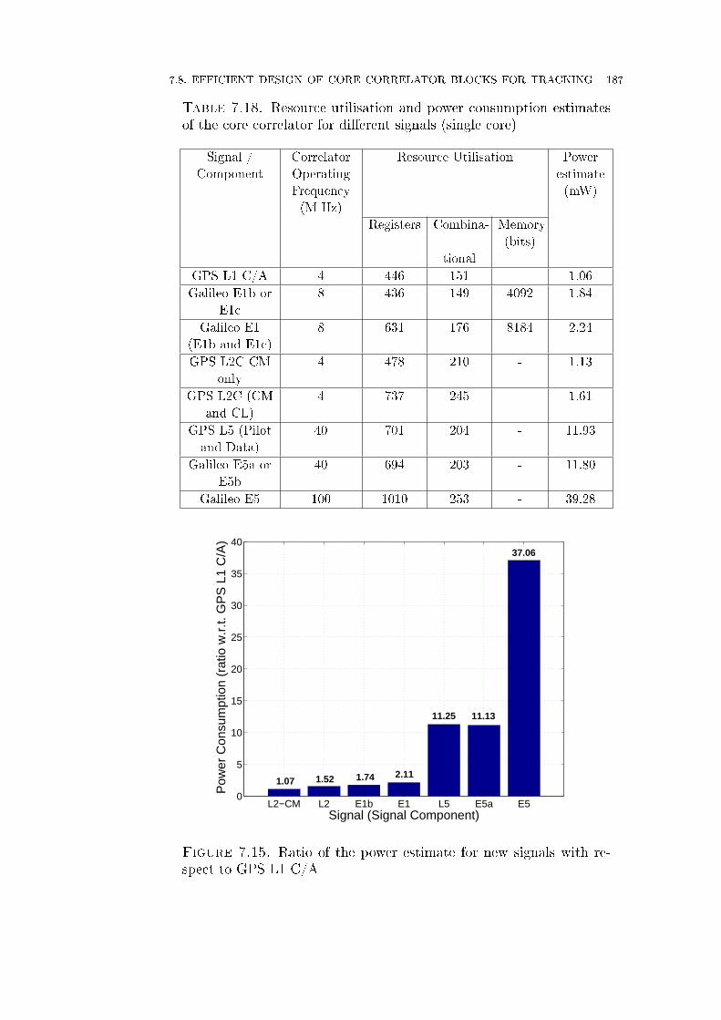
7.8. EFFICIENT DESIGN OF CORE CORRELATOR BLOCKS FOR TRACKING 187
Table 7.18. Resource utilisation and power consumption estimatesof the core correlator for di�erent signals (single core)
Signal /
Component
Correlator
Operating
Frequency
(M Hz)
Resource Utilisation Power
estimate
(mW)
Registers Combina-
tional
Memory
(bits)
GPS L1 C/A 4 446 151 - 1.06
Galileo E1b or
E1c
8 436 149 4092 1.84
Galileo E1
(E1b and E1c)
8 631 176 8184 2.24
GPS L2C CM
only
4 478 210 - 1.13
GPS L2C (CM
and CL)
4 737 245 - 1.61
GPS L5 (Pilot
and Data)
40 701 204 - 11.93
Galileo E5a or
E5b
40 694 203 - 11.80
Galileo E5 100 1010 253 - 39.28
L2−CM L2 E1b E1 L5 E5a E50
5
10
15
20
25
30
35
40
Signal (Signal Component)
Pow
er C
onsu
mpt
ion
(rat
io w
.r.t.
GP
S L
1 C
/A)
1.07 1.52 1.74 2.11
11.25 11.13
37.06
Figure 7.15. Ratio of the power estimate for new signals with re-spect to GPS L1 C/A

188 7. GALILEO E5 BASEBAND HARDWARE
of accumulators remain the same. Hence the increase in the power consumption
with respect to the L2C- CM signal is negligible.
E1b or E1c. The 10-bit shift register is absent and instead the local spreading
code is stored in memory. Hence the number of registers used is less by 10 compared
to the GPS L1 C/A. However, because of the 8 MHz sampling frequency requirement,
the power consumption increases.
E1b and E1c. Here two sets of memory codes are used each occupying 4092 bits.
In addition the local reference mixer and the accumulator need to operate on the
data of both the E1b and E1c signals. For this reason the power consumption is
close to twice that of the GPS L1 C/A.
L5 (Pilot and Data). The code generator shift register requires only 13 bits,
but the major contributors are the two signal components and the operating fre-
quency (which is 40 MHz). Hence the power consumption requirement is drastically
increased.
E5a or E5b (Pilot and Data). The code generator shift register requires only
14-bits and all the other circuit parameters remain the same as that of L5 signal.
Hence the estimated power consumption closely matches that of L5.
E5 Wideband. The code generators require only 14 bits. However, due to the
four signal components and the complex modulation the local reference mixer is
computationally intensive (more LUTs). In addition, a quadruple number of accu-
mulators are required. As mentioned earlier, independent correlation for all the four
signals is performed to allow design freedom for the subsequent stages in combining
these four components. As a result of a very high operating frequency the power
consumption shoots up to almost 37 times that of the GPS L1 C/A signal. The
power consumption for the E5 signal can be reduced a little bit further by focusing
more on how the complex mixers are realised as discussed in Chapter 8.
7.8.6. Complexity comparison results for di�erent baseband con�gu-
rations. Fig. 7.16 shows the power consumption of di�erent signals vs. the number
of channels. A �channel� comprises the core correlator, timing control, address data
multiplexer/demultiplexer (for a memory mapped interface to the subsequent stage),
and some housekeeping operations. Although the resource consumption is not de-
scribed in detail here, it should be mentioned that the two major memory spreading
code sets in the case of the Galileo signal occupy around 410K bits (E1, 4092 bits,
2 signal components, 50 satellites) of memory and 10K bits (E5 secondary code,
100 bits, 2 components, 50 satellites) which are totally new additions to the GNSS
receiver baseband hardware.
Fig. 7.17 shows the power consumption for di�erent combinations of signals
where each signal has been assumed to be using 12 channels. It is interesting to

7.9. SUMMARY 189
2 4 6 8 10 12 140
50
100
150
200
250
300
Number of channels
Pow
er c
onsu
mpt
ion
estim
ate
(mW
)
L1L2E1L5E5aE5
Figure 7.16. Power consumption of the entire baseband circuit
note that a GNSS receiver designed to process all the civilian signals of GPS and
Galileo would require slightly less than short one watt for the baseband hardware
(using the Altera Cyclone-III family device EP3C120F780C8), which is 38 times
that of GPS L1 C/A baseband hardware.
7.9. Summary
This chapter discussed the requirements for the FFT transform lengths used in
GNSS receivers to process multiple signals. The proposed method of factorising
large FFT transform lengths into smaller-point FFT blocks eliminates the need for
having separate FFTs for di�erent signals. It was demonstrated that the proposed
approach of combining the small-point blocks to build the required large FFTs pro-
vides bene�ts both in terms of reduced computational complexity and increased
resource sharing. It was also shown that for the GPS L1 C/A and Galileo E1B/C
signal combinations the reduction in complexity is about 22%. The percentage re-
duction is also high for other signal combinations.
From these results it can be concluded that the proposed approach has two
advantages:
• Code acquisition with longer codes can be achieved in practice via the FFT-based method (through the use of small-point FFT blocks) without having
to implement a FFT of large transform length.

190 7. GALILEO E5 BASEBAND HARDWARE
0 200 400 600 800 1000Power consumption estimate (mW)
Sig
nal C
ombi
natio
n
L1
L1+L2
L1+L2+E1+L5 +E5
E1+E5a
L1+E1
L5+E5a
L1+L2+L5
L1+L2+E1+L5 +E5a
L1+E1+L5+E5
E1+E5
Figure 7.17. Power consumption for di�erent multi-signal con�gurations
• Multi-band GNSS receivers can make use of small-point FFTs from a com-
mon set of building blocks, hence reducing the design complexity and in-
creasing the re-usability.
It was shown that apart from reducing the resource requirements due to the employ-
ment of the small-point FFT blocks, the Mixed-radix method of combining small-
point FFT blocks to build the large required FFT block also reduces the number of
additions and subtractions compared to the direct FFT computation method.
The proposed method does not depend on the acquisition architecture and hence
can be used in conjunction with the other two design category options (acquisition
architecture modi�cation and assistance information) to further reduce the compu-
tational burden. Apart from the reduction in the computational complexity, the
proposed method is also useful for resource sharing in a multi-band receiver.
It was shown that the use of the proposed FFT architecture reduces the com-
putational load (or number of processor cycles) and increases the re-usability of the
acquisition search engine to process di�erent signals. The proposed method is a
potential candidate for acquisition engines in future multi-band GNSS receivers.
This chapter also analysed the core correlator complexities of modernised GNSS
receiver baseband hardware. A core correlator architecture description has been
given and the number of bits for the accumulator has been derived. Power con-
sumption estimates were provided for the new signals at the core correlator level
and at the channel level.

7.9. SUMMARY 191
It was shown that a multi-frequency all-civil signal GPS and Galileo receiver
baseband hardware would consume approximately 38 times the power of a GPS L1
C/A baseband hardware. The dominant contributor to this increased complexity
and power consumption is the Galileo E5 AltBOC signal. This calls for a thoughtful
and e�cient design for future GNSS signals rather than the use of a sophisticated
signal only targetting system performance with less emphasis on receiver complexity,
and is the topic of next chapter.


CHAPTER 8
Time-Multiplexed O�set-Carrier QPSK for GNSS
8.1. Introduction
In this chapter a new method of time-multiplexing QPSK signals modulated by
complex sub-carriers is proposed. This chapter contains the work from a journal
paper currently under review (Shivaramaiah et al., 2010) in the IEEE Transactions
on Aerospace and Electronics Systems, and an extension of that manuscript's work
published in ION ITM 2011 (Shivaramaiah et al., 2011).
First, a detailed description of the new modulation scheme called Time-Multiplexed
O�set-Carrier (TMOC) QPSK is given, in which two QPSK signals are combined
to form the transmitted signal. The design of the proposed TMOC-QPSK aims
to address the complexity and power consumption issues that a receiver faces with
the constant-envelope AltBOC currently used for the Galileo E5 signal. The signal
structure is described, focusing on the signal generation methodology, power spec-
tral density and correlation function in comparison with the AltBOC modulation. A
method to realise the correlator for the proposed TMOC-QPSK signal is described
and its complexity is compared to AltBOC.
Next, a Time-Multiplexed Multi-Carrier (TMMC) modulation scheme is pro-
posed where the multiplexing scheme in TMOC is extended to accommodate more
than two QPSK signals. The potential bene�ts of using TMMC for a wideband
GNSS signal are discussed.
This chapter is organised as follows. Sec. 8.2 brie�y discusses the AltBOC
modulation complexities used for the Galileo E5 signal. Sec. 8.3 describes time-
multiplexing in the context of other GNSS signals as well as the general QPSK
modulation variants. Sec. 8.4 describes the proposed TMOC-QPSK technique as
well as its signal properties. Sec. 8.5 describes the correlator architecture for the
proposed modulation scheme, followed by an analysis of the architecture details, re-
source utilisation and power consumption in sec. 8.6. Sec. 8.7 describes an extension
of the TMOC-QPSK modulation, for use in wideband GNSS signals. Conclusions
are provided in sec. 8.8.
193
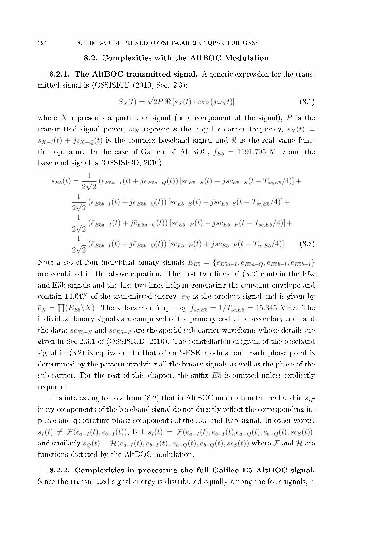
194 8. TIME-MULTIPLEXED OFFSET-CARRIER QPSK FOR GNSS
8.2. Complexities with the AltBOC Modulation
8.2.1. The AltBOC transmitted signal. A generic expression for the trans-
mitted signal is (OSSISICD (2010) Sec. 2.3):
SX(t) =√
2P < [sX(t) · exp (jωXt)] (8.1)
where X represents a particular signal (or a component of the signal), P is the
transmitted signal power, ωX represents the angular carrier frequency, sX(t) =
sX−I(t) + jsX−Q(t) is the complex baseband signal and < is the real value func-
tion operator. In the case of Galileo E5 AltBOC, fE5 = 1191.795 MHz and the
baseband signal is (OSSISICD, 2010)
sE5(t) =1
2√
2(eE5a−I(t) + jeE5a−Q(t)) [scE5−S(t)− jscE5−S(t− Tsc,E5/4)] +
1
2√
2(eE5b−I(t) + jeE5b−Q(t)) [scE5−S(t) + jscE5−S(t− Tsc,E5/4)] +
1
2√
2(eE5a−I(t) + jeE5a−Q(t)) [scE5−P (t)− jscE5−P (t− Tsc,E5/4)] +
1
2√
2(eE5b−I(t) + jeE5b−Q(t)) [scE5−P (t) + jscE5−P (t− Tsc,E5/4)] (8.2)
Note a set of four individual binary signals EE5 = {eE5a−I , eE5a−Q, eE5b−I , eE5b−I}are combined in the above equation. The �rst two lines of (8.2) contain the E5a
and E5b signals and the last two lines help in generating the constant-envelope and
contain 14.64% of the transmitted energy. eX is the product-signal and is given by
eX =∏
(EE5\X). The sub-carrier frequency fsc,E5 = 1/Tsc,E5 = 15.345 MHz. The
individual binary signals are comprised of the primary code, the secondary code and
the data; scE5−S and scE5−P are the special sub-carrier waveforms whose details are
given in Sec 2.3.1 of (OSSISICD, 2010). The constellation diagram of the baseband
signal in (8.2) is equivalent to that of an 8-PSK modulation. Each phase point is
determined by the pattern involving all the binary signals as well as the phase of the
sub-carrier. For the rest of this chapter, the su�x E5 is omitted unless explicitly
required.
It is interesting to note from (8.2) that in AltBOC modulation the real and imag-
inary components of the baseband signal do not directly re�ect the corresponding in-
phase and quadrature phase components of the E5a and E5b signal. In other words,
sI(t) 6= F(ea−I(t), eb−I(t)), but sI(t) = F(ea−I(t), eb−I(t),ea−Q(t), eb−Q(t), scS(t)),
and similarly sQ(t) = H(ea−I(t), eb−I(t), ea−Q(t), eb−Q(t), scS(t)) where F and H are
functions dictated by the AltBOC modulation.
8.2.2. Complexities in processing the full Galileo E5 AltBOC signal.
Since the transmitted signal energy is distributed equally among the four signals, it

8.2. COMPLEXITIES WITH THE ALTBOC MODULATION 195
Reference
Baseband Signal
Generator
Complex
Carrier
( )IFr t
Code
Loop
Filter
Code
NCO
,mz( )y t
( )y t
( )x t
0( ) [ ( ) ( ) ( )]y t y t y t y t
1
1( 1)
kT
k T
dt
1T
1T
,mz * ˆs t
* ˆs t
*
0ˆs t
Carrier
Loop
Filter
Carrier
discrimin
ator
Carrier
NCO
0 ( )y t 0,lz
2T
Code
discrimin
ator
Filter and
Resampler
(optional)
1
1( 1)
kT
k T
dt
2
2( 1)
kT
k T
dt
, 0, ,[ ]m m l mz z z z
Figure 8.1. A generalised tracking architecture for AltBOC signals
would be bene�cial if the received signal energy input to the acquisition or tracking
processes can be maximised by combining the individual signal components. There
are several ways to combine the signal components, each with its own advantages and
disadvantages (for details see Chapter 5). Fig. 8.1 shows an architecture where the
reference baseband signal dictates the signal component(s) tracked. The input to the
acquisition/tracking stage is assumed to be a wideband signal (> 50 MHz) centred
around 1191.795 MHz. The following is a summary of the key items that contribute
to the complexity and power consumption requirements of AltBOC receivers:
• To generate the AltBOC sub-carrier waveform scS(t) or the code modulated
sub-carrier waveform s(t), at least 4-bit amplitude quantisation is required
for a su�ciently accurate representation. This is because the values in
the sub-carrier waveform have four levels {±1.2071, ±0.5}. In addition,
due to unequal spacing between the amplitudes, anything less than 4-bit
quantisation will result in correlation loss. As mentioned in the sec. 2.11
section, using a 1-bit (two level) sub-carrier, such as those used in BOC
modulation, as a reference sub-carrier will incur about 1.38 dB correlation
loss (Soellner and Erhard, 2003).
• Multiple bits used for the sub-carrier in turn generate additional require-
ments (dealt with in detail in Sec. 8.6). First, mixing the code (or tiered
code while tracking) with the sub-carrier to generate the local reference sig-
nal requires a Look-Up-Table (LUT) instead of simple XOR logic. Second,
the reference signal shift register must carry more than 1 bit, and hence code
mixers demand either large LUTs or multipliers with adders/subtractors.
This is true even if the AltBOC code-plus-sub-carrier replica is gener-
ated like an 8-PSK constellation (OSSISICD, 2010) with output values of
{0,±0.7071,±1} which requires 4 bits. Third, the bit-width requirement
increases in the case of the wideband (or full) signal frequency domain code
acquisition technique.

196 8. TIME-MULTIPLEXED OFFSET-CARRIER QPSK FOR GNSS
e1(tk) e2(tk)
sc1(t)
s(t)
e1(tk+1) e2(tk+1)
s1(tk) s2(tk)
s(t)
s1(tk+1) s2(tk+1) sc1(tk) sc2(tk)
e(t)
s(t)
sc1(tk+1) sc2(tk+1)
t t
t
(a) (b) (c)
tk = t - kTM TM is the multiplex interval
Figure 8.2. Time-multiplexing methods to construct the basebandsignal (a) spreading codes with optional data are time-multiplexed;(b) sub-carriers are time-multiplexed; and (c) spreading codes withsub-carriers are time-multiplexed
• Even if the computational resources (logic gates in hardware or processor
load in software) can be provided in a receiver these complexities result in
a signi�cant increase in the power consumption per correlation compared
to that of a BOC modulation (as described in Chapter 7).
Since most of the parameters that trigger the complexities are related to making
the phase-multiplexing a constant-envelope signal, the next section revisits time-
multiplexing techniques to explore possibilities of creating a signal that would permit
a reduction in receiver complexity.
8.3. Time-Multiplexed Modulations
This section discusses existing time-multiplexed modulations. A �time-multiplexed
modulation� within the scope of this chapter refers to the modulation in which the
transmitted signal is constructed by time-multiplexing some or all of the compo-
nents that constitute the signal. Further, the time-multiplex operation could have
taken place at any one or more stages of the signal construction.
8.3.1. Existing time-multiplexing methods. A transmitted ranging signal
S(t) in general comprises of at least one independent stream of primary spreading
code c(t) and a carrier exp(jωt). Additional streams of primary spreading codes,
secondary or overlay codes, sub-carriers sc(t) and data d(t) may be present in the
signal. Usually, the primary code and secondary (or overlay) codes are combined
to form a tiered code and hence in this chapter, the notation c(t) is retained to
represent the tiered code as well (and distinguished appropriately when required).
As mentioned in the previous section, c(t) & d(t) constitute e(t) and the baseband
signal s(t) is constructed using e(t) and sc(t).
8.3.1.1. Time-multiplexing during the baseband signal generation. Fig. 8.2 shows
three possible time-multiplexing methods for constructing a GNSS baseband signal,
TM representing the multiplex interval. In Fig. 8.2(a), two spreading codes with
optional data are time-multiplexed and combined with the optional (the dashed box)

8.3. TIME-MULTIPLEXED MODULATIONS 197
sub-carrier. GPS L2C modulation is an example of this method with TM = Tc, the
chip period (there is no overlay code - one signal carries data, and no sub-carrier
is used). In Fig. 8.2(b), a single spreading code bit stream is combined with the
time-multiplexed sub-carrier. GPS L1C modulation is an example of this method
with TM = Tc, but the multiplex operation occurs at irregular intervals (but with
a repeated pattern of irregularity). Fig. 8.2(c) generalises (a) and (b), s1(t) and
s2(t) appropriately representing the code and sub-carrier combinations. In addition,
8.2(c) also accommodates two independent codes combined with two independent
sub-carrier streams. This last option is discussed later in detail.
8.3.1.2. Time-multiplexing during the carrier modulation. In general, the base-
band signal in GNSS is phase modulated onto the carrier using the Phase Shift
Keying (PSK) technique. A signal with a single component uses BPSK, and those
with two signal components (or two signals modulated on to the same carrier) use
QPSK. For example, the C/A code and the P(Y) codes on the GPS L1 carrier are
modulated onto the quadrature phases of the carrier, and the GPS L5 signal also
uses quadrature phases for its pilot and data signal components.
To deal with more than two signals either the number of phase points can be in-
creased or some other technique must be used. One such technique for multiplexing
three signals moves the signal energy of the third signal away from the centre such
that it does not overlap the dominant lobe of the �rst two signals. This spectral
separation requirement is one of the main reasons for adopting BOC modulation in
GNSS. The M code on the GPS L1 frequency is an example of this third signal.
For the M code the BOC (10,5) modulation was preferred mainly to enable inde-
pendent control of the power level of the L1M signal without a�ecting the C/A and
P(Y) signals. A complicated situation is encountered in situations when more than
three signals have to be combined without compromising the spectral separation
performance (Dafesh and Cahn, 2009).
Using additional frequency spectrum may not always be possible (due to fre-
quency availability or bandwidth and signal design constraints), in which case in-
creasing the number of phase points on the same carrier becomes inevitable. The
Galileo E5 signal faced this situation initially (Lestarquit et al., 2008) while trying
to combine four signal components. One of the design requirements was to exploit
the available bandwidth (~50 MHz) and at the same time ensure QPSK-like demod-
ulation of both E5a (which would allow the receivers to process E5a with GPS L5
(ISGPS705, 2010)) and E5b signals. Hence using more phase points by employing
the AltBOC modulation was the preferred choice.
In communication systems, a variant of the QPSK known as π4-QPSK has been
used (Proakis, 2000; Rappaport, 2002) to combine two QPSK signals. This is an

198 8. TIME-MULTIPLEXED OFFSET-CARRIER QPSK FOR GNSS
π/4S1=(0,0)
S2=(0,1)
S2=(1,1) S2=(1,0)
S1=(0,1)
S1=(1,1)
S1=(1,0)
may be alternate symbols of a single bit streamS1 S2and
two independent bit streamsS1 S2and
OR t
S1k
S2=(0,0)
S2k S1k+1 S2k+1 S1k+2
S2k S2k+1 S1k+2
S1k S1k+1 S1k+2
cos[ωt+Φ(S1k)] cos[ωt+Φ(S2k)] cos[ωt+Φ(S1k+1)] cos[ωt+Φ(S2k+1)]
Ts
Ts Modulated Carrier
t
Figure 8.3. Illustration of phase points in π4-QPSK modulation
alternative option to 8-PSK to obtain eight phase points. In π4-QPSK, the two sym-
bol (two-bit) streams that use QPSK have a carrier phase o�set of π4radians and a
time o�set of half a bit between them. As a result the constellation diagram resem-
bles that of the 8-PSK. Fig. 8.3 shows the phase points in a π4-QPSK modulation.
Observe that the two symbols can come from the same bit stream or di�erent bit
streams. It can be inferred from the �gure that the π4-QPSK modulation can be
considered as a time-multiplexed modulation with the time-multiplexing operation
performed during the carrier modulation. An advantage of the π4-QPSK modulation
over the 8-PSK modulation is that the successive phase change between any two
symbol transitions is limited to 135◦ instead of 180◦. As a consequence, zero cross-
ings are avoided, and hence the higher frequency components in the signal spectrum
are suppressed. This chapter makes use of a concept similar to π4-QPSK modulation,
but using sub-carriers instead of carriers.
8.3.2. Time-multiplexing example - GPS L2C. One of the constraints for
the GPS L2 civilian signal design was to place both the data and pilot components
of the signal onto the same phase of the carrier (Cheung et al., 2001; Fontana
et al., 2001). This resulted in combining the L2-CM (data carrying) and the L2-
CL (pilot) baseband signal components via a time-multiplexing method followed
by carrier modulation to form the GPS L2C signal (ISGPS200E, 2010). Other
constraints such as the spectral separation between GPS L2 M and the GPS L2C
signals also in�uenced the signal design, but the time-multiplexing methodology and
its consequences are more important in the context of this chapter.
The L2-CM and L2-CL signals are multiplexed chip-by-chip, each having a chip-
ping rate of 511.5 kHz (Fig. 8.4). Acquisition and tracking techniques have been
described in Fontana et al. (2001). It is shown in Fontana et al. (2001) that the
reduction in the chipping rate does not a�ect the code tracking performance of the
signal.

8.3. TIME-MULTIPLEXED MODULATIONS 199
CMk CLk CMk+1 CLk+1
CMk
CLk
CMk+1
CLk+1CLk-1
CMk+2
511.5 kHz CM Code eL2CM (t)
511.5 kHz CL Code eL2CL (t)
1.023 MHz L2C Code sL2C (t)
Figure 8.4. Code-multiplexing in GPS L2C signal
The baseband L2C signal can be represented in the time domain as
eL2C(t) =+∞∑
k=−∞
[cL2CM,|k|LL2CM
dL2CM,[k]NL2CMpTc,L2C/2 (t− kTc,L2C)
+cL2CL,|k|LL2CLpTc,L2C/2 (t− kTc,L2C + Tc,L2C/2)
](8.3)
=sL2C(t)
where cX,k is the kth chip of the spreading code; LX is the spreading code length;
dX,k is the kth symbol of the navigation data; NX is the number of code chips per
data symbol; Tc,X is the code chipping rate of the resultant signal (= twice the code
chipping rate of the two signal components); pT (t) is the rectangular function which
is unity from 0 < t < T and zero elsewhere; X represents the signal components L2-
CM and L2-CL in this case. Observe that the �nal baseband signal sL2C(t) = eL2C(t)
since there is no sub-carrier modulation onto the binary signal eL2C(t).
8.3.3. Time-multiplexing example - GPS L1C. The GPS L1C signal was
proposed for use in Block III satellites (Avila-Rodriguez et al., 2008) under an agree-
ment between the GPS Program O�ce and the Galileo Program O�ce. The com-
mon criterion for the Galileo E1 open service signal and the GPS L1C signal was to
transmit the signal with similar spectral characteristics using the Multiplexed Binary
O�set Carrier (MBOC) modulation technique. The mutually agreed MBOC modu-
lation dictates a power spectrum formed by combining a BOC(1,1) and a BOC(6,1)
signal with power ratio of 10/11 and 1/11 respectively (Avila-Rodriguez et al., 2008;
ISGPS800, 2010) to form the �nal signal. In the case of the Galileo E1 signal this
power requirement is handled by multiplexing the BOC(1,1) and BOC(6,1) signals
with appropriate power levels and is called a Composite BOC (CBOC) signal. More
discussions on CBOC modulation can be found in OSSISICD (2010).
Of interest in the context of this chapter is the GPS L1C signal. The pilot com-
ponent of this signal, L1C-P, adopts Time-multiplexed BOC (TMBOC) to achieve
the power spectrum properties of the MBOC modulation1(ISGPS800, 2010). Since
1Detailed theoretical background for the TMBOC and the related time multiplexing BOC modu-lations are available in Hegarty et al. (2004); Spilker (2010).

200 8. TIME-MULTIPLEXED OFFSET-CARRIER QPSK FOR GNSS
L1CPm L1CPm+2
COk COk+1 COk+2
L1CP TMBOC Sequence
COk+3 COk+4 COk+5L1CO Overlay Code (1800 bits @100 bps)
10 ms
33 Chips
L1CP Code (10230 chips @1.023 Mbps)
Time Multiplexed Subcarrier BOC (1,1) Subcarrier
BOC(6,1) Subcarrier
0 4 6 29
XOR operation
L1CPm+1
Figure 8.5. The proposed L1C pilot code generation scheme usingthe TMBOC technique
the L1C-D channel uses BOC(1,1) modulation with 25% of the total power, the L1C-
P, which uses 75% of the power employs BOC(6,1,4/33) for the time-multiplexing
scheme to achieve the desired power ratio between BOC(1,1) and BOC(6,1). Fig.8.5
illustrates the code generation scheme for the L1C-P signal. In this particular time-
multiplexing scheme the L1C-Overlay code is modulated with the time-multiplexed
sub-carrier. The time-multiplexed sub-carrier comprises 4 cycles of the BOC(6,1)
sub-carrier and 29 cycles of the BOC(1,1) sub-carrier for every 33 chips.
8.4. Time-Multiplexed O�set-Carrier QPSK : The Signal Structure
This section introduces the proposed TMOC-QPSK modulation. The signal
structure is explained by referring the task of combining four signal components. The
Galileo E5 signal components E5a-I, E5a-Q, E5b-I and E5b-Q, denoted henceforth
in this chapter as aI,aQ,bI and bQ respectively, are used as examples for the four
signal combination task.
8.4.1. Signal generation. Since two signals can be combined with QPSK
modulation, the task is now to formulate these two signals from the four that are to
be combined. A straightforward way is to combine two of these signals via a time-
multiplexing method. Under the constraint that the I and Q signal components
should occupy the in-phase and quadrature phase of the carrier and that the phase
relation between I and Q signal components should be identical for a and b signals,
there are two possibilities:
• I = TI(aI, bI) and Q = TQ(aQ, bQ) referred to as �TMOC-QPSK-ab� : in
this case, aI and aQ components are transmitted on in-phase and quadra-
ture phase respectively in the �rst (even) slot , bI and bQ components are
transmitted on in-phase and quadrature phase respectively in the second
(odd) slot; and

8.4. TIME-MULTIPLEXED OFFSET-CARRIER QPSK : THE SIGNAL STRUCTURE 201
eP1(tk) eP2(tk) eP1(tk+1) eP2(tk+1)
Subcarrier
TC
ePx(t)
scL(tk) scH(tk) scL(tk+1) scH(tk+1)
eP1(tk) eP2(tk) eP1(tk+1)ePx(t) eP2(tk+1)
scL(tk)Subcarrier
TC
s(t)= sI(t) +j sQ(t)
scH(tk) scL(tk+1) scH(tk+1)
(a) TMOC-QPSK-ab
(b) TMOC-QPSK-IQ
(c) Subcarrier Waveform
eD1(tk) eD2(tk) eD1(tk+1)eDy(t) eD2(tk+1)
scL(tk)Subcarrier
TC
scH(tk) scL(tk+1) scH(tk+1)
eD2(tk) eD1(tk) eD2(tk+1) eD1(tk+1)
Subcarrier
TC
eDy(t)
scH(tk) scL(tk) scH(tk+1) scH(tk+1)
scL(t) = sc(t) – j sc(t-Tsc/4) = scI(t) – j scQ(t)
scH(t) = sc(t) + j sc(t-Tsc/4) = scI(t) + j scQ(t)
x,y {1,2}
x,y {1,2}
s(t)= sI(t) +j sQ(t)
sc(t)1
-1
0Tsc
sco(t)1
-1
0TSC
(d) π/4 phase shifted Subcarrier
Tsc /2 Tsc /2Tsc /8
Figure 8.6. Time-multiplexing methods and the corresponding sub-carrier waveform: (a) TMOC-QPSK-ab multiplexing method; (b)TMOC-QPSK-IQ; (c) one cycle of sub-carrier waveform
• a = Ta(aI, aQ) and b = Tb(bI, bQ) referred to as �TMOC-QPSK-IQ�: in
this case, aI and bI components are transmitted on in-phase and quadra-
ture phase respectively in the �rst (even) slot, bQ and aQ components are
transmitted on in-phase and quadrature phase respectively in the second
(odd) slot;
where Ta, Tb, TI , TQ are the functions representing the time-multiplexing operations
with the requirement of an ordered pair of signal components as the parameters. In
order to avoid low frequency inter-modulation components, chip-by-chip multiplex-
ing has been used in the case of the L2C signal, and the same approach is adopted
for the proposed time-multiplexing method. In addition it is assumed that all four
signal components possess similar properties (code length, chipping rate and indi-
vidual signal transmit power) as in the case of the Galileo E5 signal components.
This allows the use of an identical time-multiplexing method for both the groupings
i.e. Ta= T b = TI = TQ = T . (Note: It not a necessary condition that all four signal
components possess similar properties but further discussion is beyond of the scope
of this thesis). Fig. 8.6 shows the two multiplexing schemes in detail, tk is used as a
time parameter to represent one chip duration of the corresponding signal. It is clear
that the TMOC-QPSK-ab method would result in an alternating spectrum corre-

202 8. TIME-MULTIPLEXED OFFSET-CARRIER QPSK FOR GNSS
sponding to the a and b signals. In other words, a and b signals, when considered
individually, will have discontinuities in the time domain. However the duration of
this discontinuity depends on the chipping rate. When the chipping rate is high,
for example 10.23 MHz as in the Galileo E5a or E5b signal, the RF front-end can
still see the signal as nearly-continuous because the typical Automatic Gain Control
(AGC) time constant is much higher than 97.75ns (i.e. 110.236
) (Zarlink, 1999). In the
TMOC-QPSK-IQ method, the pilot signals are time-multiplexed with each other
(the other group has data signals).
8.4.1.1. TMOC-π4-QPSK : a variant of the TMOC-QPSK. It is possible to make
use of eight phases of the sub-carrier with the TMOC-QPSK method. In TMOC-π4-QPSK, the time-multiplexing scheme is exactly the same as the corresponding
TMOC-QPSK method but the sub-carrier phase assignments for the signal compo-
nents in odd slots are shifted by π4. This is equivalent to advancing the sub-carrier
phase by a factor of π4, i.e. sco(t) = sc(t). exp(j π
4) = sc(t + Tsc
8) (see Fig. 8.6). The
advantage of TMOC-π4-QPSK is that successive sub-carrier phase changes between
the even and odd chips are limited to 135 degrees instead of 180 degrees for the
TMOC-QPSK method.
8.4.2. Signal representation, phase assignments and the transmitted
signal. The generalised complex baseband TMOC-QPSK signal for a combination
of four signal components (assuming two data and two pilot signal components) can
be written as
s(t) =1
2√
2eP1(t)
[sc(t)− jsc(t− Tsc
4)
]+
1
2√
2· jeD1(t)
[sc(t)− jsc(t− Tsc
4)
]+
1
2√
2eP2(t)
[sc(t) + jsc(t− Tsc
4)
]+
1
2√
2· jeD2(t)
[sc(t) + jsc(t− Tsc
4)
](8.4)
where
ePx(t) =+∞∑
k=−∞
cPx,|k|LCpTM/2 (t− kTM) , x ∈ {1, 2}
eDy(t) =+∞∑
k=−∞
cDy,|k|LCdy,|k|NC pTM/2 (t− kTc + TM/2) , y ∈ {1, 2} (8.5)
where e• represents the spreading code with optional data, su�xes P and D denote
the pilot and data respectively, sc(t) denotes the sub-carrier with period Tsc, TM is
the multiplex interval and Tc is the chip period. Observe from (8.4) and (8.5) that
the TMOC-QPSK-ab is achieved when x = y and TMOC-QPSK-IQ is achieved
when x 6= y. In the case of TMOC-π4-QPSK, s(t) should be replaced with sco(t).
The transmitted signal equation and the constellation diagram are shown in Fig. 8.7.

8.4. TIME-MULTIPLEXED OFFSET-CARRIER QPSK : THE SIGNAL STRUCTURE 203
Time Slot
Even Chip
Odd Chip
Transmitted Signal S(t)
sI(t) cos(jωct+Φ) - sQ(t) sin(jωct+Φ)
sI(t) cos(jωct+Φ) - sQ(t) sin(jωct+Φ)
SubcarrierUsed
(a) TMOC-QPSK
sc(t)
sc(t)
Time Slot
Even Chip
Odd Chip
Transmitted Signal S(t)
sI(t) cos(jωct+Φ) - sQ(t) sin(jωct+Φ)
sI(t) cos(jωct+Φ) - sQ(t) sin(jωct+Φ)
SubcarrierUsed
(b) TMOC-π/4-QPSK
sc(t)
sc(t+Tsc/8)
Figure 8.7. TMOC-QPSK and TMOC-π4-QPSK transmitted signal
Table 8.1 lists the phase assignments that results from a TMOC-QPSK modulation.
It can be observed that only four phases are used due to the time-multiplexing
method.
8.4.2.1. Nomenclature. In line with the AltBOC modulation, the TMOC-QPSK
modulation described in this chapter is denoted as TMOC-QPSK(m,n), e.g. TMOC-
QPSK(15,10) meaning fsc = 15.345 MHz and fco = 10.230 MHz.
8.4.3. Power spectral density. The power spectral density (PSD) of a constant-
envelope AltBOC signal is given in Rebeyrol et al. (2005), and repeated here for com-
pleteness. For 2fscfco
odd, the normalised PSD of the constant-envelope AltBOC(m,n)
is given by
GAltBOC(f) =4
π2f 2Tc
cos2(πfTc)
cos2(πf Tsc2
)(8.6)[
cos2
(πf
Tsc2
)− cos
(πf
Tsc2
)− 2 cos
(πf
Tsc2
)cos
(πf
Tsc4
)+ 2
]The TMOC-QPSK essentially contains a sine-phased sub-carrier and a cosine-phased
sub-carrier. This is because (see Fig. 8.6) if the in-phase sub-carrier component
scI(t) corresponds to the cosine sub-carrier, scQ(t) = sc(t − Tsc4
) corresponds to
the sine sub-carrier. In other words, this is equivalent to the spectrum of a non-
constant-envelope AltBOC (AltBOC-NCE). The PSD of a TMOC-QPSK signal can
be obtained by combining the PSDs of Sine-BOC and Cosine-BOC (Betz, Winter
2001-2002; Rebeyrol et al., 2005). Thus for 2fscfco
odd the PSD of TMOC-QPSK(m,n)
is given by (Appendix J):
GTMOC−QPSK(f) =4
π2f 2Tc
cos2(πfTc)
cos2(πf Tsc2
)
[sin2
(πf
Tsc2
)+
{cos
(πf
Tsc2
)− 1
}2]
(8.7)
For the TMOC-π4-QPSK signal, the sub-carrier in the alternate slots are phase
shifted by π4w.r.t their phases in the preceding slots. The equation for the PSD of a

204 8. TIME-MULTIPLEXED OFFSET-CARRIER QPSK FOR GNSSTable8.1.Tran
smitted
sub-carrier
signal
phases
intheprop
osedmodulation
Meth
od
TMOC-Q
PSK-IQ
/TMOC-π4 -Q
PSK-IQ
TMOC-Q
PSK-ab
/TMOC-π4 -Q
PSK-ab
aI
11
-1-1
--
--
11
-1-1
--
--
bQ1
-11
-1-
--
--
--
-1
-11
-1bI
--
--
11
-1-1
--
--
11
-1-1
aQ
--
--
1-1
1-1
1-1
1-1
--
--
Even
chip
sc=1
π47π4
3π4
5π4
--
--
π47π4
3π4
5π4
--
--
sc=-1
5π4
3π4
7π4
π4-
--
-5π4
3π4
7π4
π4-
--
-Oddchip
sc=1
--
--
π47π4
3π4
5π4
--
--
π47π4
3π4
5π4
sc=-1
--
--
5π4
3π4
7π4
π4-
--
-5π4
3π4
7π4
π4
Oddchip
sc=1
--
--
π22π
π3π2
--
--
π22π
π3π2
π4 -QPSK
sc=-1
--
--
3π2
π2π
π2-
--
-3π2
π2π
π2
Even
chip
constella-tion
E5aI
E5bI
E5aI
E5aQ
Oddchip
constella-tion
E5bQ
E5aQ
E5bI
E5bQ
Oddchip
constellation
π4 -QPSK
E5bQ
E5aQ
E5bI
E5bQ

8.4. TIME-MULTIPLEXED OFFSET-CARRIER QPSK : THE SIGNAL STRUCTURE 205
−100 −50 0 50 100−110
−105
−100
−95
−90
−85
−80
−75
−70
−65
−60
Frequency (MHz)
Pow
er/fr
eque
ncy
(dB
/Hz)
AltBOCAltBOC−NCETMOC−QPSKTMOC−pi/4−QPSK
Figure 8.8. PSD of the AltBOC, AltBOC-NCE, TMOC-QPSK andTMOC-π
4-QPSK; analytical
TMOC-π4-QPSK(m,n) signal when 2fsc
fcois odd (derived in Appendix J) is given by:
GTMOC−QPSK(f) =2
π2f 2Tc
cos2(πfTc)
cos2(πf Tsc2
)
[sin2
(πf
Tsc2
)+
{cos
(πf
Tsc2
)− 1
}2
+ cos2
(πf
Tsc2
)− 2 cos
(πf
Tsc2
)cos
(πf
Tsc4
)+ 1
](8.8)
Fig. 8.8 plots (8.6),(8.7) and(8.8) for the case with fco = 10.23 MHz and fsc = 15.345
MHz (i.e. 2fscfco
= 3). In Fig. 8.9 the PSD is plotted for the three types of signals
simulated using the GIOVE-B primary and secondary codes. It is interesting to note
that the magnitude spectrum of the AltBOC(15,10) and the TMOC-π4-QPSK(15,10)
match very closely; this is because both the modulations are making use of eight
phases. However, as explained in the previous section, in TMOC-π4-QPSK all the
spectrum energy is due to the four component signals only (i.e. does not include
any product signals).
8.4.4. Transmit power level. It is evident from the previous sections that it
is possible to keep the total transmit power level for the TMOC-QPSK modulation
the same as the AltBOC modulation, and hence at the receiver utilise the complete
transmit power - as opposed to AltBOC which loses 15% due to the product signal
component. Table 8.2 compares the transmit power levels of AltBOC and TMOC-
QPSK signals assuming that the wideband AltBOC signal transmitted power is
100%.

206 8. TIME-MULTIPLEXED OFFSET-CARRIER QPSK FOR GNSS
−100 −50 0 50 100−100
−95
−90
−85
−80
−75
−70
−65
−60
Frequency (MHz)
Pow
er/fr
eque
ncy
(dB
/Hz)
Welch Power Spectral Density Estimate
AltBOCAltBOC−NCETMOC−QPSKTMOC−pi/4−QPSK
Figure 8.9. PSD of the AltBOC, AltBOC-NCE, TMOC-QPSK andTMOC-π
4-QPSK; simulation
Table 8.2. Comparison of relative transmit signal power levels
Signal
Component /
Modulation
AltBOC TMOC-QPSK-ab TMOC-QPSK-IQ
Wideband
Signal
100% 100% 100%
aI 21.34% 25% (even chip
50%, odd chip
0%)
25% (even chip 50%,
odd chip 0%)
aQ 21.34% 25% (even chip 50%,
odd chip 0%)
25% (even chip 0%,
odd chip 50%)
bI 21.34% 25% (even chip 0%,
odd chip 50%)
25% (even chip 0%,
odd chip 50%)
bQ 21.34% 25% (even chip 0%,
odd chip 50%)
25% (even chip 50%,
odd chip 0%)
a (aI and aQ) 42.68% 50% (even chip 100%,
odd chip 0%)
50% (even chip 50%,
odd chip 50%)
b (bI and bQ) 42.68% 50% (even chip 0%,
odd chip 100%)
50% (even chip 50%,
odd chip 50%)
both a and b 85.36% 100% 100%

8.5. CORRELATOR ARCHITECTURE FOR THE TMOC-QPSK SIGNAL 207
Carrier Generator
( )IFr t
( )IF dj te
Carrier Mixer
Code Mixer
Ref. signal Generator
ˆ( )s t
ˆ( )ks t 1
ˆ( )ks t
( )kx t1( )kx t ( )x t
ˆ( )s t
( ) ( )k ks t n t( )x t contains 1 1( ) ( )k ks t n t
Code mixer input
Reference signal
( )x t
2Tc
Even/Odd Chip Select (EOCS)
( )y t I Accumulator Q Accumulator
Corr. Values
Figure 8.10. Correlator architecture to process the widebandTMOC-QPSK signal
8.5. Correlator Architecture for the TMOC-QPSK Signal
This section describes the correlator architectures for processing the TMOC-
QPSK signal and compares the correlator output with that of the AltBOC modu-
lation, both for wideband processing and sideband processing.
8.5.1. Correlator architecture : wideband processing. Fig. 8.10 shows
the architecture to process the wideband TMOC-QPSK signal, with all lines carrying
complex signals. The signal at IF plus associated Doppler is mixed with the local
carrier to obtain the baseband signal x(t), which comprises two sidebands separated
at equal spacings from the centre (zero frequency plus any residual Doppler) and
carries both a and b signal components. The reference signal generates s(t− τ) and
comprises the code and the sub-carrier. The Even/Odd Chip Select (EOCS) is a
gating signal of duration Tc used to select the reference signal a or b. The complex
code mixer multiplies the signal to produce y(t) which is fed to the accumulators.
The detailed implementation of the reference signal generator and code mixer is
described in the next section.
8.5.2. Correlator output and the correlation waveform : wideband
processing. The received IF signal for a particular satellite employing a complex
sub-carrier modulation (AltBOC or TMOC-QPSK) can be written as:
rIF (t) =√
2Pr [sI(t− τ) cos (ωIF t+ ωdt+ θ)− sQ(t− τ) sin (ωIF t+ ωdt+ θ)]+nW (t)
(8.9)
where Pr = A2
2is the power, τ is the delay (s), θ is the phase (rad) and ωd is
the Doppler frequency (rad/s) of the received signal and nW is the additive white
Gaussian noise with two-sided power spectral density N0
2W/Hz. The carrier signal

208 8. TIME-MULTIPLEXED OFFSET-CARRIER QPSK FOR GNSS
√2 exp
[−j(ωIF t+ ωdt+ θ
)]generated in the receiver with the estimated Doppler
ωd and the estimated phase θ is mixed with rIF (t) to obtain:
x(t) =A√2{[sI(t− τ) cos (∆ωdt+ ∆θ)− sQ(t− τ) sin (∆ωdt+ ∆θ)]
j [sQ(t− τ) cos (∆ωdt+ ∆θ) + sQ(t− τ) sin (∆ωdt+ ∆θ)]}+ nI(t) + jnQ(t)
(8.10)
where ∆ωd = ωd − ωd and ∆θ = θ − θ . The local reference signal generated is
s(t− τ) = sI(t− τ)− jsQ(t− τ). The signal s(t) di�ers from s(t) due to the absence
of secondary codes and the data. However, assuming that the correlation opera-
tion is considered within one secondary code period (or data bit period whichever
is minimum) allows one to write s(t− τ) = s∗(t− τ) where ∗ denotes the conjugateoperation (see Chapter 5). The output of the reference signal mixer y(t) is accumu-
lated (typically over one code period duration) to obtain the correlation result. The
output of the accumulator is (see Appendix K for the derivation):
zk+ =√
2ATcohR (∆τ)Rsc (∆τ) sinc
(∆ωd
Tcoh2
)ej∆θ +R′ + n′ (t) (8.11)
where R (∆τ) denotes the autocorrelation of the codes (all four codes are assumed
to have equal autocorrelation values), Rsc (∆τ), the sub-carrier correlation denotes
the combined correlation of the sub-carrier component pairs, R′ contains the cross
correlation noise contributed by all the code pairs, n′(t) contains the noise terms
obtained via the mixing operation of nI(t) + jnQ(t) with s∗(t− τ), Tcoh = LTc is the
coherent integration duration and L is the primary code length.
For the TMOC-QPSK and the TMOC-π4-QPSK modulations the equation for
the output of the correlator remains the same as in (8.11) except that the sub-
carrier correlation is di�erent. The number of autocorrelation and the number of
cross correlation terms remain the same. The sub-carrier correlation for the AltBOC
modulation Rsc,AltBOC (∆τ) is provided in (K.5) in Appendix K. It is the task now to
derive the sub-carrier correlation for the two modulations. The complete derivations
of all the terms have been carried out individually for all the three modulations, but
only the results are discussed here.
8.5.2.1. Incoming and reference sub-carrier correlations in TMOC-QPSK. In
this case, the sub-carrier is a complex square wave, i.e. sc(t) can be written as
sc(t) = sgn (cos (ωsct)) + j sgn (sin (ωsct)). Moreover, the correlation between the
sub-carrier phases are equal because integration of the product of both the cosine and
sine square wave functions yields a triangular function. Following the same proce-
dure as for the AltBOC modulation described in Appendix K, Rsc,TMOC−QPSK (∆τ)

8.5. CORRELATOR ARCHITECTURE FOR THE TMOC-QPSK SIGNAL 209
is found to be:
Rsc,TMOC−QPSK (∆τ) = 8RscI ,scI (∆τ) (8.12)
8.5.2.2. Incoming and reference sub-carrier correlations in TMOC-π4-QPSK. In
TMOC-π4-QPSK, there are essentially two sets of sub-carriers. The �rst set used
in even numbered slots is the same as the sub-carriers used in TMOC-QPSK. The
second set used in the odd numbered slots is o�set by π4rads with respect to. the
�rst set and is given by sco(t) = sgn(cos(ωsct+ π
4
))+ j sgn
(sin(ωsct+ π
4
)). The
sub-carrier correlation contains the correlation due to eight pairs RscI ,scI , RscQ,scQ ,
RscoI ,scoI , RscoQ,scoQ , RscI ,scoI , RscQ,scoQ , RscoI ,scI and RscoQ,scQ . Since the correlation
depends on the relative phase shift, the �rst four pairs are the same. In the last four
pairs, there are two types, one with the phase advance and the other with the phase
delay, and hence result in corresponding phase shifted triangular waves. Finally,
Rsc,TMOC−π4−QPSK (∆τ) is found to be:
Rsc,TMOC−π4−QPSK (∆τ) = 4RscI ,scI + 2RscI ,scoI + 2RscoI ,scI (8.13)
The sub-carrier correlations for all three types of modulations are plotted in Fig.
8.11. Rsc,AltBOC (∆τ) is the correlation between two quantised cosine waves and re-
sembles a smoothed triangular wave. Rsc,TMOC−QPSK (∆τ) is the correlation of pairs
of square waves and is a triangular wave. Rsc,TMOC−π4−QPSK (∆τ) not only resembles
a smoother triangular wave, but also closely matches the sub-carrier correlations of
the AltBOC modulation. The Alternate Linear O�set Carrier (AltLOC) uses Sine
and Cosine sub-carriers and hence the cosine waveform (which is the correlation be-
tween incoming and the reference sub-carrier) is shown for reference. Observe that
the cosine function serves as a good approximation for all three sub-carrier types.
8.5.3. Correlator output waveform : wideband processing. Fig. 8.12
shows the normalised auto-correlation waveforms of the modulations under consid-
eration. Observe that the auto-correlation waveform of TMOC-QPSK matches that
of the AltBOC-NCE and the auto-correlation waveform of TMOC-π4-QPSK matches
that of the AltBOC. At the boundaries (close to +1 or -1 chip shifts) the AltBOC
and TMOC-π4-QPSK exhibit peaks of very low magnitude which are absent in the
TMOC-QPSK. This is justi�ed by noting that those small peaks are also absent in
the autocorrelation waveform of AltBOC-NCE. The di�erences in autocorrelation
values among the modulations are greatly reduced when the �ltering is considered,
as shown in Fig. 8.13.
8.5.4. Correlator architecture : independent sideband processing. Be-
cause the spectrum of the TMOC-QPSK signal closely resembles the AltBOC signal,
the individual signals can be obtained following the same procedure as in the Al-
tBOC case (the following discussion applies to TMOC-π4-QPSK as well). That is,

210 8. TIME-MULTIPLEXED OFFSET-CARRIER QPSK FOR GNSS
−1.5 −1 −0.5 0 0.5 1 1.5−1
−0.8
−0.6
−0.4
−0.2
0
0.2
0.4
0.6
0.8
1
Time delay in number of subcarrier cycles
Nor
mal
ized
Cor
rela
tion
Val
ue
AltBOCTMOC−QPSKTMOC−pi/4−QPSKAltLOC
Figure 8.11. Incoming and reference sub-carrier correlations for Al-tBOC, TMOC-QPSK, TMOC-π
4-QPSK and AltLOC modulations
−2 −1.5 −1 −0.5 0 0.5 1 1.5 2−0.8
−0.6
−0.4
−0.2
0
0.2
0.4
0.6
0.8
1
1.2
Chip Shift
Nor
mal
ized
Aut
ocor
rela
tion
Val
ue
AltBOCAltBOC−NCETMOC−QPSKTMOC−pi/4−QPSK
Figure 8.12. Normalised auto-correlation waveforms ofAltBOC,TMOC-QPSK,TMOC-π
4-QPSK and AltBOC-NCE; in�-
nite bandwidth; simulation

8.5. CORRELATOR ARCHITECTURE FOR THE TMOC-QPSK SIGNAL 211
−2 −1.5 −1 −0.5 0 0.5 1 1.5 2−0.6
−0.4
−0.2
0
0.2
0.4
0.6
0.8
1
Chip Shift
Nor
mal
ized
Aut
ocor
rela
tion
Val
ue
AltBOCAltBOC−NCETMOC−QPSKTMOC−pi/4−QPSK
Figure 8.13. Normalised auto-correlation waveforms ofAltBOC,TMOC-QPSK,TMOC-π
4-QPSK and AltBOC-NCE; 50
MHz bandwidth; simulation
the signal components a and b can be obtained by translating the individual bands
to an appropriate IF (or zero-IF) and then treating them as QPSK signals. The
e�ect of time-multiplexing is that the �signal-plus-noise� and �noise-only� alternate
with every chip slot in the case of TMOC-QPSK-ab, as seen from the centre of
any one sideband. However this e�ect is absent in the case of TMOC-QPSK-IQ as
the spectrum is either always occupied by the I or the Q signal component. Fig.
8.14 shows a correlator architecture for obtaining the individual signals a and b
independent of each other; all lines carry complex signals. In Fig. 8.14(a), the re-
ceived IF version of the TMOC-QPSK-ab signal is mixed with the locally generated
carrier at a frequency of ωIF + ωd ± ωsc, where the sign used for the sub-carrier
frequency in the equation determines whether signal a is being processed or signal
b. The resultant signal x(t) contains the baseband signal (with residual Doppler)
and noise components without any sub-carrier. The signal-plus-noise component
e′a(t) = ea(t) + n(t) {or e
′
b(t) = eb(t) + n(t)} and the noise-only term n(t) alternate
between chips. The gating signal �Code Enable� (CEN) will ensure the exclusion of
the noise-only component during the correlation process.
The correlator in Fig. 8.14(b) is suitable for the TMOC-QPSK-IQ modulation
and follows the same process as in the case of TMOC-QPSK-ab for the carrier re-
moval. The di�erence would be in the code mixing stage where individual I and
Q code enable signals (ICEN and QCEN respectively) are used to enable the cor-
responding code mixing and the subsequent accumulation path. Observe from Fig.
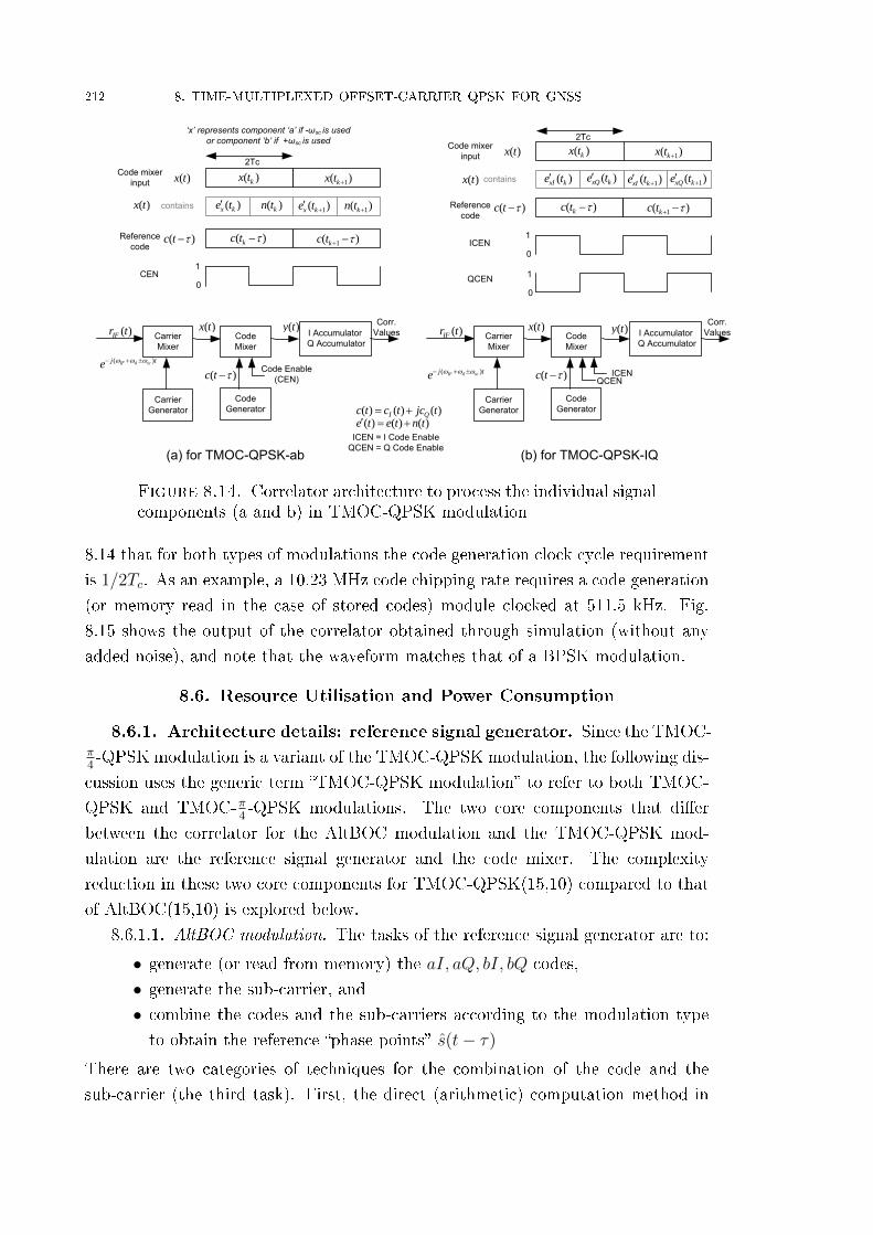
212 8. TIME-MULTIPLEXED OFFSET-CARRIER QPSK FOR GNSS
Carrier Generator
( )IFr t
( )IF d scj te
Carrier Mixer
Code Mixer
Code Generator
( )c t
( ) ( ) ( )( ) ( ) ( )
I Qc t c t jc te t e t n t
Code Enable (CEN)
I Accumulator Q Accumulator
Carrier Generator
( )IFr t
( )IF d scj te
Carrier Mixer
Code Mixer
Code Generator
( )c t ICENQCEN
ICEN = I Code Enable QCEN = Q Code Enable(a) for TMOC-QPSK-ab (b) for TMOC-QPSK-IQ
( )kc t 1( )kc t
1
0
1
0
( )kx t1( )kx t ( )x t
( )c t
( )xI ke t( )x t contains ( )xQ ke t1( )xI ke t
1( )xQ ke t
Code mixer input
Reference code
ICEN
QCEN
( )kc t 1( )kc t
1
0
( )kx t1( )kx t ( )x t
( )c t
( )x ke t( )x t contains ( )kn t1( )x ke t
1( )kn t
Code mixer input
Reference code
CEN
‘x’ represents component ‘a’ if -ωsc is used or component ‘b’ if +ωsc is used
( )x t ( )x t
2Tc
2Tc
Corr. Values( )y t ( )y t I Accumulator
Q Accumulator
Corr. Values
Figure 8.14. Correlator architecture to process the individual signalcomponents (a and b) in TMOC-QPSK modulation
8.14 that for both types of modulations the code generation clock cycle requirement
is 1/2Tc. As an example, a 10.23 MHz code chipping rate requires a code generation
(or memory read in the case of stored codes) module clocked at 511.5 kHz. Fig.
8.15 shows the output of the correlator obtained through simulation (without any
added noise), and note that the waveform matches that of a BPSK modulation.
8.6. Resource Utilisation and Power Consumption
8.6.1. Architecture details: reference signal generator. Since the TMOC-π4-QPSK modulation is a variant of the TMOC-QPSK modulation, the following dis-
cussion uses the generic term �TMOC-QPSK modulation� to refer to both TMOC-
QPSK and TMOC-π4-QPSK modulations. The two core components that di�er
between the correlator for the AltBOC modulation and the TMOC-QPSK mod-
ulation are the reference signal generator and the code mixer. The complexity
reduction in these two core components for TMOC-QPSK(15,10) compared to that
of AltBOC(15,10) is explored below.
8.6.1.1. AltBOC modulation. The tasks of the reference signal generator are to:
• generate (or read from memory) the aI, aQ, bI, bQ codes,
• generate the sub-carrier, and• combine the codes and the sub-carriers according to the modulation type
to obtain the reference �phase points� s(t− τ)
There are two categories of techniques for the combination of the code and the
sub-carrier (the third task). First, the direct (arithmetic) computation method in

8.6. RESOURCE UTILISATION AND POWER CONSUMPTION 213
−2 −1.5 −1 −0.5 0 0.5 1 1.5 2−0.2
0
0.2
0.4
0.6
0.8
1
Chip Shift
Nor
mal
ized
Cor
rela
tion
Val
ue
’a’ Component’b’ Component
Figure 8.15. Output of the correlator for independent sideband pro-cessing; simulation
which the complex code and the complex sub-carrier are multiplied to obtain the
complex output s(t − τ). This method is suitable for software implementations,
e.g. Matlab/C on a desktop or embedded processor. Since �oating point arithmetic
is expensive in terms of computation, scaled integer arithmetic often replaces such
computations. Fig. 8.16 shows the direct computation method of generating the
reference signal in the case of AltBOC(15,10). The �rst two troughs of the scaled
integer approximation error function result in representing the values taken by the
sub-carrier as {±2,±5} and {±5,±12} with errors of 3.5% and 0.6% respectively
(tables of di�erent representations and errors are provided in Appendix L). Hence
the complex multiplication operation results in eight sign change operations on 4 (or
5)-bit numbers and four addition/subtraction operations on 6 (or 7)-bit numbers.
Even if the �rst approximation is chosen, 6 bits are required to accommodate the
result. This is an enormous amount of computation compared, to say, a complex
BOC(m,n) modulation case where the result is 1 bit and two XOR gates (one each
for I and Q) are required to combine the code and the sub-carrier. (Note: to simplify
the discussion this model omits the product-signal components and incurs a 14.64%
loss in received signal energy; including the product-signal components would further
increase the computation requirements.)
The second method is the Look-Up-Table (LUT) method, better suited for hard-
ware implementations, e.g. in an FPGA or an ASIC. (Note: the LUT method can
also be used in software implementations especially for an embedded processor, but
often it is not the choice for higher level programming languages.) Fig. 8.17 shows

214 8. TIME-MULTIPLEXED OFFSET-CARRIER QPSK FOR GNSS
-1
Codes
+1
-0.5Subcarriers
+1.2071
0.5
-1.2071
Operation ( )( ) ( )( )aI aQ I Q bI bQ I Qc jc sc jsc c jc sc jsc
Integer Arithmetic
(Approximation #1)
Integer Arithmetic
(Approximation #2)
±1 (2 bits)
{±0.5, ±1.2071}
~= {±2, ±5}
=> 4 bits
3.5% error
±1 (2 bits)
{±0.5, ±1.2071}
~= {±5, ±12}
=> 5 bits
0.6% error
Max. I & Q result
= ±20 => 6 bits
Max. I & Q result
= ±48 => 7 bitsEight sign change operations on 4(or 5)-bit numbers,
Four add/sub operations on 6(or 7)-bit numbers
Figure 8.16. Direct computation method of AltBOC reference sig-nal generation
AltBOC
Modulat
ion
Sub-carrier
NCO
ˆ ˆ( ) ( )I Qs t js t aI
aQ
bI
bQ
cc
cc
3 MS bits
(subcarrier phase)
{0, ±0.7071, ±1}
Arithmetic Representation
(Approximation #1)
{0, ±0.7071, ±1} ~=
{0, ±2, ±3} => 3 bits
5.7% error
Arithmetic Representation
(Approximation #2)
{0, ±0.7071, ±1} ~=
{0, ±5, ±7} => 4 bits
1% error
128x3
128x3
LUT
128x4
128x4
LUT
Mapped Representation of
Approximation #2
{0, ±5, ±7}
=> 5 levels
=> 3 bits
128x3
128x3
LUT
Two 128x3 LUTs Two 128x4 LUTs Two 128x3 LUTs
Figure 8.17. LUT method of AltBOC reference signal generation
the LUT method of AltBOC signal generation. OSSISICD (2010) suggests this
method because it is comparatively simple to implement. The three most signif-
icant (MS) bits of the sub-carrier NCO (which represent the eight phases of the
sub-carrier) and the four codes act as address inputs to the LUT. The output (in-
cluding the product components) can be represented using approximated integer
arithmetic. Representing {0,±0.7071,±1} as {0,±5,±7} incurs only 1% error but
requires 4 bits (Appendix L). In most situations, the code mixer which is the next
stage is also implemented as a LUT and hence s(t− τ) which is an input to the code
mixer, does not require true value representation (see sec. (7.8)). The third option
for mapping the values can now be presented. Since there are only 5 levels, 3 bits
are su�cient to represent s(t− τ). As a result, the LUT method requires two (one
for I and one for Q) 128x3 LUTs. This requirement is also very expensive compared
to a complex BOC(m,n) case.
8.6.1.2. TMOC-QPSK modulation. Fig. 8.18 illustrates the direct computation
method of generating the reference signal. The sub-carriers in the TMOC-QPSK
modulation are two-valued and hence logical representation is possible. s(t − τ)
requires only 1 bit for the representation, and, interestingly the computation load is
just four 3-bit XOR gates (two for each I and Q). Additional two 2 bit XOR gates
are required to incorporate the EOCS signal. The LUT method of implementation
shown in Fig. 8.19 would be an overkill for the TMOC-QPSK modulation, as
it requires a 128x1 LUT. The sub-carrier phase identi�cation in TMOC-π4-QPSK

8.6. RESOURCE UTILISATION AND POWER CONSUMPTION 215
-1
Codes
+1
Subcarriers
Operation ˆ +
ˆ + I aI I bI I
Q aQ Q bQ Q
s c EOCS sc c EOCS sc
s c EOCS sc c EOCS sc
Logical
Representation
1,0 => 1-bit
I and Q result
1-bit
-1
+1
1,0 => 1-bit
0
EOCS
1
1,0 => 1-bit
Four 3-bit XOR operations, Two 2-bit XOR operations
Figure 8.18. Direct computation method of TMOC-QPSK referencesignal generation
TMOC-
QPSK
Modulat
ion
Sub-carrier
NCO
ˆ ˆ( ) ( )I Qs t js t aI
aQ
bI
bQ
cc
cc
2 MS bits
(subcarrier phase)
{±1}
Logical Representation
(Also a mapped representation)
±1 => 0,1 =>
1-bit
128x1
128x1
LUT
Even/Odd Chip
Select (EOCS)
Two 128x1 LUTs
Figure 8.19. LUT method of TMOC-QPSK reference signal generation
requires 3 MS-bits, however the amplitude is still represented using 1 bit and hence
the size of the LUT does not change.
8.6.1.3. Implications for architectures for correlation in the frequency domain.
Reducing the number of bits in the local reference signal has a huge impact on the
architectures that employ the frequency domain approach for correlation. Usually,
computing the FFT of the reference signal is required as part of the frequency domain
correlation approach. It is well known (Oppenheim and Schafer, 1998) that the
number of guard bits necessary to compensate for the maximum possible bit growth
for an N-point FFT is log2N + 1. Given that the code length of AltBOC signals is
10230, a 10230-point FFT requires 14 guard bits. A 2-bit input (representing ±1,
which would be the case for TMOC-QPSK signal) will require 16-bit words for the
FFT. On the other hand, for the AltBOC case, 20-bit words would be required and
this results in a larger footprint.
8.6.2. Architecture details: Code mixer. For a 2-bit IF signal representing
the levels {±1,±3} and a 2-bit local carrier representing {±1,±2}, the carrier mixer
output will be {±1,±2,±3,±6} requiring 4 bits for an arithmetic representation and

216 8. TIME-MULTIPLEXED OFFSET-CARRIER QPSK FOR GNSS
Code Mixer
ˆ( )s t
( )x t{±1,±2,±3,±6}
(4 bits)
Max. ±20 (6 bits)
Six Multiplications, Ten Additions/Subtractions
Max. ±240 (9 bits)
Code Mixer
ˆ( )s t
( )x t
{±1,±2,±3,±6}(8 levels, 3 bits)
{0, ±5, ±7} (5 levels, 3 bits)
Four 64x8 LUTs, Two Addition/Subtractions
Max. ±84 (8 bits)
(a) Direct (Arithmetic) Computation Method (b) LUT Method
I Accumulator Q Accumulator
Correlation Values
Correlation Values( )y t ( )y t I Accumulator
Q Accumulator
Figure 8.20. Direct computation and LUT method of code mixerimplementation in AltBOC modulation
Code Mixer
ˆ( )s t
( )x t{±1,±2,±3,±6}
(4 bits)
1-bit
Four sign change operations, Two Additions/Subtractions
Max. ±12 (5 bits)
Code Mixer
ˆ( )s t
( )x t
{±1,±2,±3,±6}(8 levels, 3 bits)
1-bit
Four 16x3 LUTs, Two Additions/Subtractions
Max. ±12 (5 bits)
(a) Direct (Arithmetic) Computation Method (b) LUT Method
I AccumulatorQ Accumulator
Correlation Values
Correlation Values( )y t ( )y t I Accumulator
Q Accumulator
Figure 8.21. Code mixing operation in TMOC-QPSK modulation
3 bits (eight levels) for a mapped representation (see Chapter 7). The direct com-
putation method and the LUT method of code mixing for the AltBOC modulation
are shown in Fig. 8.20. If the reference signal generation uses an arithmetic rep-
resentation then the code mixer must use the direct computation method, and in
that case the code mixer requires six multiplications and ten addition/subtraction
operations (two complex multiplications, one each for I and Q). In the case of the
LUT method, four 64x8 tables are required. The output of the code mixer, y(t)
grows to 8 bits, thus resulting in wider accumulators to obtain the correlation val-
ues (note: the accumulators have to accumulate a large number of samples; typically
the duration is one code period). In the case of TMOC-QPSK it is interesting to
note that the computation is greatly reduced (Fig. 8.21). Given that for the wide-
band AltBOC(15,10), the number of samples per integration period is very high due
to a high sampling frequency, the lower bit-width requirement for y(t) results in a
signi�cant advantage over the AltBOC modulation.
8.6.2.1. Correlator with multiple taps. In the architecture discussions in this sec-
tion, the role of the shift register has not been explicitly mentioned. However, when
the correlator is used for tracking the signal, the delay locked loops require more
than one tap, typically three; the �early�, the �prompt� and the �late�. For this
reason, s(t− τ) will be a 3-element vector (for the early, prompt and late reference
signals) and the bit-width of the shift registers is a�ected by the number of bits used
to represent the reference signal. As a result, the requirement of the number of code
mixers and the number of accumulators also increases.

8.6. RESOURCE UTILISATION AND POWER CONSUMPTION 217
Table 8.3. Correlator complexity comparison summary for AltBOCand TMOC-QPSK modulations
AltBOC TMOC-QPSK
Ref.signalgen-erator
DirectCom-puta-tion
8 sign changeops, 4
Add/Sub(excludingthe product-
signalgeneration)
Four 3-bitXOR, two2-bit XOR
LUTMethod
Two 128x3LUTs
Two 128x1LUTs
Code mixer DirectCom-puta-tion
6 Mult, 10Add/Sub
4 signchange ops,2 Add/Sub
LUTMethod
Four 64x8LUTs, 2Add/Sub
Four 16x3LUTs, 2Add/Sub
Table 8.4. Logic resource and estimated power consumption for Al-tBOC and TMOC-QPSK correlators
Number of Logic Elements Power Con-sumptionEstimate
AltBOC 1186 31.98 mWTMOC-QPSK 802 24.59 mW% Reduction 32.37 23.10
8.6.3. Complexity comparison summary. Table 8.3 summarises the com-
parison and highlights (in green) the best options to realise the reference signal gen-
erator and the code mixer in both the AltBOC modulation and the TMOC-QPSK
modulation.
8.6.4. Hardware resource utilisation and power consumption estimate.
In order to gain more insight into the complexity reductions the correlators for the
AltBOC and TMOC-QPSK modulations were implemented on a Altera Cyclone-
III FPGA. With the help of Altera's Power Play Power Analyzer tool the power
consumption for both types of modulations were estimated and are listed in Table
8.4. Best options (minimum resource, those highlighted in Table 8.3) were chosen
to implement the reference signal generator and the code mixer.

218 8. TIME-MULTIPLEXED OFFSET-CARRIER QPSK FOR GNSS
8.7. On E�cient Wideband GNSS Signal Design
This section aims at extending the TMOC-QPSK signal to e�ciently utilise a
given bandwidth. This modulation, referred to as Time-Multiplexed Multi-Carrier
(TMMC), divides the available bandwidth intoN sub-bands such that each sub-band
resembles a Quadrature Phase Shift Keying (QPSK) modulation and at the same
time allows the receiver to exploit the bene�ts of a wideband signal. The generation
of the new signal and its properties are described. The bene�ts of using TMMC
modulation for wideband signals in order to overcome the errors due to propagation
channel impairments, continuous wave interference mitigation and receiver design
complexity is discussed.
8.7.1. Wideband GNSS signals.
8.7.1.1. How wide is a wideband signal? Since this chapter deals with wideband
signals, it is necessary to discuss what bandwidth can be referred to as �wideband�
in the context of GNSS or more generally, in the context of navigation and ranging
signals.
The accuracy of the position, velocity and time solution in GNSS depends on
many factors, both internal and external to the system. The internal error sources
are from the space, ground and control segments of GNSS and the rest arise form
external factors, such as the atmosphere and other ground-based systems that in-
terfere with GNSS. Let these errors be grouped into two categories, those that are
attributed to the �signal structure� and those that are not. In general, wideband
signals o�er better performance than narrowband signals. As the signal bandwidth
increases, there would be a �breakeven point� around which the errors due to the
signal structure are comparable to the combined contribution of all other errors.
Beyond the breakeven bandwidth the errors due to the signal structure diminish
further (though it may asymptotically reach a constant, eventually), but the other
errors remain the almost the same. It can be argued that the wideband signals are
the signals whose bandwidth is greater than this breakeven bandwidth.
As an example, consider the GPS L1 C/A code signal, which has a certain
multipath-free code ranging accuracy, certain multipath performance. etc., which
can be attributed to the signal structure. Consider a hypothetical signal �L1 X�
in the same system, that has ten times the signal bandwidth (only the dominant
frequency lobes) compared to the GPS L1 C/A but at the same carrier frequency.
Further, assume that the L1 X signal o�ers better ranging accuracy and multipath
mitigation capabilities that result in lower code ranging errors compared to the L1
C/A. However, the L1 X signal experiences almost the same errors as does the L1
C/A due to the ground segment, the ionosphere, etc., that are not related to the
signal structure. Assuming a breakeven bandwidth of 20MHz, the GPS L1 C/A

8.7. ON EFFICIENT WIDEBAND GNSS SIGNAL DESIGN 219
can be considered a narrowband signal and the L1 X can be considered a wideband
signal. The discussions in this chapter continue this assumption of 20MHz as the
breakeven bandwidth.
8.7.1.2. Drawbacks of current wideband GNSS signal modulations. A given fre-
quency band can be used to transmit one of the several possible variants of the
existing signals. For example, assuming an integer multiple of 1.023MHz for the
code chipping rate, a bandwidth of 20.46MHz can accommodate any of the follow-
ing modulations: BPSK(10), BOC(5,5), BOC(6,4), BOC(8,2), BOC(9,1) or any of
the AltBOC counterparts of the corresponding BOC (details will be provided later in
this section, see Fig. (8.22)). However, each of these options has its own advantages
and disadvantages. On the one hand BPSK(10) with a 10.23MHz spreading code
occupies the entire band, o�ers a simple correlation function but is more prone to
continuous wave (CW) interference. On the other hand AltBOC(9,1) has dominant
lobes present at the boundaries of the spectrum which can be independently de-
modulated. This allows the receiver to mitigate CW interference to some extent (by
excluding the interference-a�ected lobe, resulting in only half of the signal energy
being used) but su�ers from the problem of several strong correlation side-peaks.
Considering AltBOC modulation as an example, it was discussed in Chapter
6 that the total group delay error due to signal propagation (including that due
to multipath) as seen from the centre of the band (E5 signal in this case) can
be compensated for by estimating the di�erential phase delays of two equidistant
points from the centre (E5a and E5b in this case). In other words, independently
demodulating and estimating the phase delays of QPSK signals like those on the E5a
and E5b bands can help in compensating for the group delay error of the AltBOC
E5 signal. The two-point estimate is a trivial solution and cannot address the second
order errors. Moreover having several such virtually independent sub-bands allows
a receiver to isolate the interference-a�ected sub-bands.
Hence the modulation options mentioned in the previous paragraph do not o�er
any signi�cant advantage in dealing with frequency selective channel impairments.
The Time-Multiplexed Multi-Carrier modulation introduced in this chapter can be
used to generate a wideband signal that has the potential to address these drawbacks.
8.7.1.3. Desired signal modulation type and properties. The question now is : is
it possible to have a signal within the 20.46MHz bandwidth that has the following
features?
• The signal should have several sub-bands, that can be independently de-
modulated as QPSK(1) signals and also as a wideband signal,
• a combination of the ten QPSK(1) signals or the single whole signal should
produce a narrow correlation triangle with suppressed side-peaks,

220 8. TIME-MULTIPLEXED OFFSET-CARRIER QPSK FOR GNSS
• the baseband signal should o�er a constant-envelope when the individual
sub-bands are combined onto a single central carrier at the transmitter,
• the sub-bands should not interfere with each other, and
• processing the signal, especially the baseband signal processing, should be
simple and relatively inexpensive.
The AltBOC modulation currently used for the Galileo E5 signal exhibits features
similar to the above for a two sub-band case. Hence it would be wise to use AltBOC
as a starting point. However, extending the AltBOC modulation scheme to include
more than two sub-bands (i.e. using more than one complex sub-carrier) a�ects the
constant-envelope property. This is because all the components should be combined
onto one single central carrier so as to use a single transmit ampli�er, and the
combination of several components result in varying amplitudes in the complex
plane. Even if there is a possibility to obtain a constant-envelope, the sub-carrier
waveform design becomes extremely di�cult. In other words, the AltBOC type of
modulation is not scalable.
8.7.2. Some wideband signal candidates with AltBOC modulation.
Within a given bandwidth the AltBOC modulation can be used to accommodate
some of the signals that satisfy at least a sub-set of the desired signal features. In-
vestigating these signals will provide an insight into the gap between the desired
signal and AltBOC.
The AltBOC(m,n) modulation results in two dominant frequency lobes with
null-null bandwidth 2 · fco Hz and 2mn− 2 suppressed frequency lobes with null-null
bandwidth fco Hz. Thus a bandwidth of B Hz can be used to accommodate any
AltBOC signal that satis�es the criterion m = B2·1.023e6
− n, with the constraint of n
and m to be integers and B to be a multiple of fco.
Fig. 8.22 shows the possible AltBOC signals within a 20.46MHz bandwidth
(�rst two dominant lobes) choosing n to be an integer. The BPSK(10) modulation
is also shown for reference. The correlation functions for the two extreme cases
AltBOC(5,5) and AltBOC(9,1) are shown in Fig. 8.23.
As mentioned in sec. (8.7.1), although AltBOC(9,1) provides a narrow corre-
lation peak, there are several side-peaks. This is due to the fact that the useful
information in AltBOC(9,1) is contained only in the two 2.046MHz lobes at the
extreme ends of the band and hence that modulation does not e�ciently utilise
the entire spectrum. On the other hand, AltBOC(5,5) is closer in its features to
BPSK(10) due to the presence of wide frequency lobes which are more prone to
interference, though the spectrum usage is more e�cient compared to AltBOC(9,1).
The next section discusses a multi-carrier modulation that combines the bene�ts of

8.7. ON EFFICIENT WIDEBAND GNSS SIGNAL DESIGN 221
−10 −5 0 5 10−85
−80
−75
−70
−65
−60
−55
Frequency (MHz)
Pow
er/F
requ
ency
(dB
/Hz)
BPSK(10)AltBOC(5,5)AltBOC(6,4)AltBOC(7.5,2.5)AltBOC(8,2)AltBOC(9,1)
Figure 8.22. Possible AltBOC signals within a 20.46MHz band
−2 −1.5 −1 −0.5 0 0.5 1 1.5 2−0.8
−0.6
−0.4
−0.2
0
0.2
0.4
0.6
0.8
1
Chip Shift
Nor
mal
ized
Aut
ocor
rela
tion
Val
ue
BPSK(10)AltBOC(5,5)AltBOC(9,1)
Figure 8.23. Correlation functions for BPSK(10), AltBOC(5,5) andAltBOC(9,1)

222 8. TIME-MULTIPLEXED OFFSET-CARRIER QPSK FOR GNSS
−10 −5 0 5 10−85
−80
−75
−70
−65
−60
−55
Frequency (MHz)
Pow
er/F
requ
ency
(dB
/Hz)
AltBOC(1,1)AltBOC(3,1)AltBOC(5,1)AltBOC(7,1)AltBOC(9,1)
Figure 8.24. A 20.46MHz band used with AltBOC variants; odd m
better spectral usage and at the same time preserves a narrow correlation function
with suppressed side-peaks.
8.7.3. Multi-carrier modulation. The multi-carrier actually refers to the use
of more than one sub-carrier, and the �sub-� is left out - this is also the case for modu-
lation schemes used in other wireless communication systems (Pun et al., 2007). The
use of multiple sub-carriers seeks to �ll the gaps in the frequency spectrum within the
given bandwidth. The time-multiplexing technique aims to generate a signal that
uses multiple sub-carriers, which is otherwise not possible with the AltBOC mod-
ulation. This section explains the proposed multi-carrier modulation and the next
section describes the generation of the proposed signal using a time-multiplexing
method.
Instead of the AltBOC modulation �lling in the whole of the given bandwidth
with one signal, it is possible to use the given bandwidth in smaller non-overlapping
portions, each portion used by one signal. This is the basis of the requirement
that the desired signal should allow independent demodulation of smaller portions
of itself (how it can be �independently� demodulated will be discussed later in this
chapter). To do this one can start from the AltBOC(1,1) signal which �lls the
4.092MHz (-2.046MHz to +2.046MHz) at the centre of the given 20.46MHz band.
Next, the AltBOC(3,1) signal places its dominant lobes beyond 4.092MHz, and now
the coverage is (including the �rst signal) -4.092MHz to +4.092MHz. This can be
continued until the whole of the 20.46MHz is occupied by dominant lobes of di�erent
AltBOC variants.
Fig. 8.24 shows the spectrum obtained with all the variants with �odd� m from
AltBOC(1,1) to AltBOC(9,1) such that the dominant lobes do not overlap. This
non-overlapping is a constraint at this stage because the individual signals should

8.7. ON EFFICIENT WIDEBAND GNSS SIGNAL DESIGN 223
−2 −1.5 −1 −0.5 0 0.5 1 1.5 2−0.5
0
0.5
1
Chip Shift
Nor
mal
ized
Aut
ocor
rela
tion
Val
ue
AltBOC(1,1)+AltBOC(3,1)+AltBOC(5,1)+AltBOC(7,1)+AltBOC(9,1)BPSK(10)
Figure 8.25. Combined correlation waveform of AltBOC variants; odd m
−10 −5 0 5 10−85
−80
−75
−70
−65
−60
−55
Frequency (MHz)
Pow
er/F
requ
ency
(dB
/Hz)
AltBOC(2,1)AltBOC(4,1)AltBOC(6,1)AltBOC(8,1)
Figure 8.26. A 20.46MHz band used with AltBOC variants; even m
not interfere with each other (later in the chapter it will be shown that the time-
multiplexing eliminates this constraint). Now it is of interest to look into the corre-
lation waveform of the signal which combines all these individual signals. Fig. 8.25
shows the correlation waveform along with that of BPSK(10) for reference. Observe
that the correlation main peak is narrow, but there are two side-peaks at a distance
of 0.5 chips.
Instead of using the odd values for m the other option is to use �even� values for
m which gives AltBOC(2,1) to AltBOC(8,1) signals. The power spectral densities
are shown in Fig. 8.26 and the correlation waveform obtained by combining the
signals is shown in Fig. 8.27.
Observe again that the main correlation peak is narrow but there are two side-
peaks at 0.5 chip o�sets. The combination of odd m variants or the even m variants

224 8. TIME-MULTIPLEXED OFFSET-CARRIER QPSK FOR GNSS
−2 −1.5 −1 −0.5 0 0.5 1 1.5 2−0.4
−0.2
0
0.2
0.4
0.6
0.8
1
1.2
Chip Shift
Nor
mal
ized
Aut
ocor
rela
tion
Val
ue
AltBOC(2,1)+AltBOC(4,1)+AltBOC(6,1)+AltBOC(8,1)BPSK(10)
Figure 8.27. Combined correlation waveform of AltBOC variants; even m
−10 −5 0 5 10−85
−80
−75
−70
−65
−60
−55
Frequency (MHz)
Pow
er/F
requ
ency
(dB
/Hz)
AltBOC(1,1)AltBOC(2,1)AltBOC(3,1)AltBOC(4,1)AltBOC(5,1)AltBOC(6,1)AltBOC(7,1)AltBOC(8,1)AltBOC(9,1)
Figure 8.28. A 20.46MHz band used with AltBOC variants; bothodd and even m
produce side-peaks because there is still the gap between the dominant lobes of
the signals. However, there is a di�erence, the side-peaks in the odd type have a
negative correlation value, and they are positive in the case of the even type. The
very next option would be to combine both the types, thus having all the variants
from AltBOC(1,1) to AltBOC(9,1) and allowing the overlap of dominant lobes. Fig.
8.28 shows the power spectral density and Fig. 8.29 shows the correlation waveform
of combining all the odd and even variants.
Observe now that the side-peaks have been highly suppressed and also that

8.7. ON EFFICIENT WIDEBAND GNSS SIGNAL DESIGN 225
−2 −1.5 −1 −0.5 0 0.5 1 1.5 2−0.2
0
0.2
0.4
0.6
0.8
1
1.2
Chip Shift
Nor
mal
ized
Aut
ocor
rela
tion
Val
ue
BPSK(10)AltBOC(1,1)+AltBOC(2,1)+AltBOC(3,1)+AltBOC(4,1)+AltBOC(5,1)+AltBOC(6,1)+AltBOC(7,1)+AltBOC(8,1)+AltBOC(9,1)
Figure 8.29. Combined correlation waveform of all AltBOC vari-ants; both odd and even m
the correlation main peak is narrower than that of the BPSK(10). The centre
2.046MHz (assuming a similar overlap like other lobes in the spectrum) of the band
is still un�lled, but this would require a BPSK(1) modulation unlike other sub-
bands which are the byproducts of AltBOC modulation. Interestingly, BPSK(1)
modulation can be treated as AltBOC(0.5,1) and hence becomes a speci�c case of
the AltBOC modulation. The AltBOC(0.5,1) signal is included as the tenth signal
and the correlation waveform is only slightly altered (not plotted in the �gures in
this chapter) with the addition of this signal. Hence, the total number of sub-bands
becomes 19 and the total number of signals is now 10.
This section used the term �combined� without going into details of how the
individual signals are combined. The next section discusses a time-multiplexing
method to realise the combination of individual signals.
At this point it is worth mentioning that the ideal spectrum for the desired signal
would have a rectangular shape in the power spectral density, which means almost
no gap between the sub-bands. Realisation of such a signal would require a very high
number of sub-bands (in other words sub-carriers) like those used in other wireless
communication systems and the feasibility of generation of such a signal has to be
studied in detail, which is beyond the current scope of this thesis.
8.7.4. Time-multiplexed multi-carrier modulation. One of the require-
ments for the desired signal is to ensure that there is little or no interference between
sub-bands. However the previous section discussed the bene�ts of overlapping the
sub-bands in suppressing the side-peaks. Avoiding interference by using di�erent
spreading codes for di�erent side-bands (say one code for one sub-carrier) would
have two issues at the outset. First, the cross-correlation between the codes will not

226 8. TIME-MULTIPLEXED OFFSET-CARRIER QPSK FOR GNSS
AltBOC (5,1)
exp{ jq(k)ωc(t-kTc) }
q=[-4 4], k = [0 8], q,k Ƶ
Multiplexedsignal
Figure 8.30. AltBOC(5,1) covering a 20.46MHz band in the �scantype� time-multiplexing
be eliminated completely just outside the dominant lobe, and may lead to correla-
tion sub-peaks (Issler et al., 2003). Second, the requirement for numerous spreading
codes that should be employed increases as the number of side-bands increases. For
these reasons, multiplexing the individual signals in time would be is a good option
to explore further.
A method of multiplexing the individual signals for a single complex sub-carrier
(two side-bands), with the example of replacing the AltBOC modulation, has been
proposed earlier in this chapter.
There are many ways to realise the multi-carrier signal whose spectrum is shown
in Fig. 8.28. This section describes three straightforward schemes.
8.7.4.1. AltBOC signals are time-multiplexed. The sub-bands can be time-multip
-lexed, chip-by-chip, one sub-band pair at a time, if each pair uses the constant-
envelope AltBOC modulation.
Case 1. Spread type: The sequence of signals transmitted in this case is Al-
tBOC(1,1), AltBOC(2,1), AltBOC(3,1), AltBOC(4,1), AltBOC(5,1), Al-
tBOC(6,1), AltBOC(7,1), AltBOC(8,1), AltBOC(9,1), and then this se-
quence repeats for the next chip. This is called �spread type� because in
the frequency domain, the sequence of side-bands transmitted follows the
two �nger points of a �spread� operation on a touchscreen device.
Case 2. Scan type: In this case, only AltBOC(5,1) modulation is used for all
the sub-band pairs. In the �rst slot, AltBOC(5,1) is multiplied by a -4MHz
complex tone to shift the baseband signal such that the left dominant lobe
occupies the space of leftmost desired signal lobe. In the second slot the
translation is -3MHz, and so on up to +4MHz in the ninth slot. This process
is depicted in Fig. 8.30.
However, doing so requires four spreading codes and a multi-level sub-carrier wave-
form. Since one of the requirements is to reduce receiver complexity it would be
preferable to use a simple two-level (square wave) sub-carrier waveform and to use

8.7. ON EFFICIENT WIDEBAND GNSS SIGNAL DESIGN 227
eP(t)
sc1LSubcarrier
TC
s(t)= sI(t) +j sQ(t)
sc1H sc2L sc2H
eD(t)
TC
Subcarrier
+ =
eP(tk+1)
scNH sc1L sc1H
eD(tk+1)
2NTC
scNL
sciL= sci(t)-jsci(t-Tsci/4) sciH= sci(t)+jsci(t-Tsci/4)
eP(tk)
eD(tk)
sc1L sc1H sc2L sc2H scNH sc1L sc1HscNL
Figure 8.31. An illustration of time-multiplexing with multiple sub-carriers: �spread type�
only two spreading codes, one for the I channel and the other for the Q channel. This
leads to a scheme of extending TMOC-QPSK to multiplex the sub-bands, instead
of AltBOC.
8.7.4.2. TMOC-QPSK signals are time-multiplexed. TMOC-QPSK can be used
instead of AltBOC in the two cases similar to those ones mentioned in the previous
sub-section.
Case 1. Spread type: Fig. 8.31 shows the time-multiplexing considering N
complex sub-carriers (2N sub-bands). The sequence illustrated in Fig. 8.31
results in transmitting TMOC-QPSK(1,1), TMOC-QPSK(2,1), TMOC-QPSK
(3,1), ..., TMOC-QPSK(9,1), and then the sequence repeats.
Case 2. Scan type: A variant of the above method is also possible where the
two bands in the TMOC-QPSK pair are not transmitted one after the other.
In this case the sequence of multiplexing is sequential when viewed from the
frequency domain perspective. Fig. 8.32 shows the �scan type� of time-
multiplexing considering N complex sub-carriers (2N sub-bands or 2N + 1
sub-bands if BPSK(1) signal is also included). The sequence can be written
as QPSK−9(1), QPSK−8(1),...,QPSK−1(1), QPSK1(1),QPSK2(1),...,QPSK9(1),
where the subscript denotes the multiplier (in multiples of fcerror is reduced)
used to o�set of the QPSK signal from the centre of the band. Observe that
the sequence is repeated after all the sub-carriers are used.
8.7.4.3. Nomenclature. TMMC can be identi�ed with the bandwidth (B) and
the chipping frequency (fco) of the individual components, both represented as in-
teger multipliers of 1.023MHz. For example, the 20.46MHz bandwidth, 1.023MHz
chipping frequency case considered in the previous sections, which is implemented

228 8. TIME-MULTIPLEXED OFFSET-CARRIER QPSK FOR GNSS
eP(t)
sc9LSubcarrier
TC
s(t)= sI(t) +j sQ(t)
sc8L sc(N-1)H
eD(t)
TC
Subcarrier
+ =
eP(tk+1)
scNH sc9L
eD(tk+1)
2NTC
sciL= sci(t)-jsci(t-Tsci/4) sciH= sci(t)+jsci(t-Tsci/4)
eP(tk)
eD(tk)
sc1L sc8L
sc9L sc8L sc(N-1)H scNH sc9L sc8L
scNHsc1H sc2H
sc1L sc1H sc2H
Figure 8.32. An illustration of time-multiplexing with multiple sub-carriers: �scan type�
Tc
c(t)
Re [sc(t)]
Figure 8.33. Code and sub-carrier for a partial sequence ofTMMC(10,1); only the real component of the complex sub-carrieris shown
with 10 sub-carriers (including the AltBOC(0.5,1) signal) signal with 19 sub-bands
of 2.046MHz width (with 1.023MHz overlap between sub-bands) is represented as
TMMC(10,1).
8.7.4.4. Receiver baseband signal processing. This section discusses a method to
acquire and track a TMMC signal, speci�cally TMMC(10,1). During the discussion,
BPSK(10) with (I and Q channels) and AltBOC(5,5) are referred to when necessary
to emphasise the di�erences.
Acquiring the complete signal: The acquisition of a TMMC(10,1) signal
requires the generation of one spreading code and nine sub-carrier waveforms as
shown in Fig. 8.33.
Acquiring individual sub-bands: Individual sub-bands can be acquired by
translating the desired band to baseband (frequency translation) and then corre-
lating with the local spreading code. However, any one particular sub-band is not
continuous in time, for example, QPSK−5 will only be present in every 5th slot and
repeats every 18 slots (19 slots if the BPSK(1) is also included). This is not a prob-
lem for three reasons: (i) the same spreading code is used for all the sub-bands; (ii)

8.7. ON EFFICIENT WIDEBAND GNSS SIGNAL DESIGN 229
0 10 20 30 40 50 60−2.5
−2
−1.5
−1
−0.5
0
0.5
1
1.5
2
2.5
Multipath delay (m)
Cod
e m
ultip
ath
erro
r (m
)
Code multipath error comparison, SMR = 6dB
E5a−20MHz; δ=0.15TMMC(10,1)−20MHz; δ=0.15
Figure 8.34. Comparison of code multipath error-envelope forTMMC(10,1) and BPSK(10) signals
the local code repeats in each slot; and (iii) the time-multiplexing is carried out chip-
by-chip. As a result the only issue is that the initial code phase ambiguity due to
time-multiplexing is up to one chip duration and has to be resolved. A non-coherent
combination of all the individually acquired sub-bands will produce a BPSK(1)-like
correlation waveform.
8.7.5. Potential performance bene�ts of using TMMC for wideband
signals.
8.7.5.1. Code multipath error envelope comparison. Fig. 8.34 shows the code
multipath error-envelope for BPSK(10) and TMMC(10,1) signals. Observe that
even though the error for low multipath delays is reduced, there are oscillations
in the error-envelope for multipath delays beyond one chip duration. This is also
evident from the correlation waveform in Fig. 8.29. This is one drawback of the
TMMC modulation that needs to be addressed in future work.
8.7.5.2. Continuous wave (CW) interference. When the signal is a�ected by
narrow-band CW interference only the sub-band where the CW interference is
present, sideband would have the signal strength attenuated, as illustrated in Fig.
8.35. In the worst case if the frequency of the CW interference happens to lie midway
between two sub-bands, then two sub-bands will be a�ected. Since any one sub-
band has 1/19th of the total weight in a TMMC(10,1), the total signal degradation
due to one CW interfering tone will be approximately 5.2% or about 0.47dB in the
best case and about 0.95dB in the worst case. When there is knowledge about the
sub-band being a�ected, the local code/sub-carrier portion for that sub-band could
be initialised to zeros, thus avoiding any noise creeping into the processing. When
there is no knowledge about the a�ected sub-band, it is also possible to compare the

230 8. TIME-MULTIPLEXED OFFSET-CARRIER QPSK FOR GNSS
CW Interference
Figure 8.35. Illustration of CW interference a�ecting only one sub-band
signal strengths of all the sub-bands by tracking the individual sub-bands. This may
allow the receiver to isolate that particular sub-band. However tracking individual
sub-bands may lead to additional processing requirements.
8.7.5.3. DME/TACAN interference. The DME/TACAN interference is known
to be present in the L5/E5 band and occurs at multiples of 1MHz. It is interesting
to note that if the centre of the band is aligned to a frequency mid-way between the
1MHz boundary (i.e. the centre frequency is not a multiple of 1MHz) then all the
multiples of 1MHz frequencies will coincide with the centre of the gap that exists
between the sub-bands in the TMMC(10,1). However, design practice in GNSSs
will allow only integer multiples of 10.23MHz to be chosen as carrier frequencies.
For example the L5 carrier frequency is 1176.45MHz, which is 115 x 10.23MHz. So
in this example there is only a slight o�set between the 0.5MHz and 0.45MHz and
the interfering frequency will be �just inside� the 3dB bandwidth of any sub-band,
which is better than the interfering signal a�ecting the peak of the frequency lobe.
This situation is illustrated in Fig. 8.36.
8.7.5.4. Frequency selective propagation delay distortion. GNSS signals su�er
from several types of propagation delay distortions. Some of the distortions that
seriously a�ect the ranging performance are frequency dependent, ionosphere and
multipath being the two major sources.
The ionosphere causes phase advances and time delays for signals that travel
through it. The ionosphere delay is inversely proportional to the square of the carrier
frequency of the signal. When there are multiple carriers within a wideband signal,
the parameter of interest is the ionosphere dispersion. Signals with a bandwidth
of 20.46MHz at about 1.2GHz carrier frequency experience a dispersion of about
0.34 metres for a 10m ionosphere delay up to 3.4 metres for a 100m ionosphere
delay. For a 51.15MHz signal these dispersion values become about 0.85 m and
about 8.5 m respectively. The code measurement noise standard deviation for a
20.46MHz BPSK(10) signal is about 0.28 meters (Sleewaegen et al., 2004). For
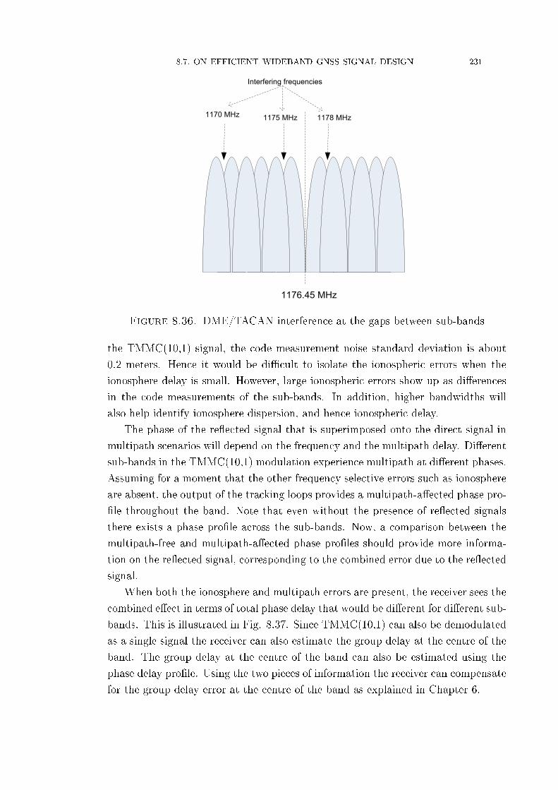
8.7. ON EFFICIENT WIDEBAND GNSS SIGNAL DESIGN 231
1176.45 MHz
1175 MHz 1178 MHz1170 MHz
Interfering frequencies
Figure 8.36. DME/TACAN interference at the gaps between sub-bands
the TMMC(10,1) signal, the code measurement noise standard deviation is about
0.2 meters. Hence it would be di�cult to isolate the ionospheric errors when the
ionosphere delay is small. However, large ionospheric errors show up as di�erences
in the code measurements of the sub-bands. In addition, higher bandwidths will
also help identify ionosphere dispersion, and hence ionospheric delay.
The phase of the re�ected signal that is superimposed onto the direct signal in
multipath scenarios will depend on the frequency and the multipath delay. Di�erent
sub-bands in the TMMC(10,1) modulation experience multipath at di�erent phases.
Assuming for a moment that the other frequency selective errors such as ionosphere
are absent, the output of the tracking loops provides a multipath-a�ected phase pro-
�le throughout the band. Note that even without the presence of re�ected signals
there exists a phase pro�le across the sub-bands. Now, a comparison between the
multipath-free and multipath-a�ected phase pro�les should provide more informa-
tion on the re�ected signal, corresponding to the combined error due to the re�ected
signal.
When both the ionosphere and multipath errors are present, the receiver sees the
combined e�ect in terms of total phase delay that would be di�erent for di�erent sub-
bands. This is illustrated in Fig. 8.37. Since TMMC(10,1) can also be demodulated
as a single signal the receiver can also estimate the group delay at the centre of the
band. The group delay at the centre of the band can also be estimated using the
phase delay pro�le. Using the two pieces of information the receiver can compensate
for the group delay error at the centre of the band as explained in Chapter 6.

232 8. TIME-MULTIPLEXED OFFSET-CARRIER QPSK FOR GNSS
Pha
se d
elay
Figure 8.37. Illustration of forming a phase delay pro�le with theaim of aiding the compensation of group delay at the centre of theband.
8.8. Summary
A new constant-envelope modulation technique TMOC-QPSK, and its vari-
ant TMOC-π4-QPSK, which use a time-multiplexing method to combine complex
sub-carrier modulated spreading codes were presented in this chapter. The power
spectral density and correlation function of TMOC-QPSK and TMOC-π4-QPSK are
shown to match that of the non-constant-envelope AltBOC and constant-envelope
AltBOC respectively. The TMOC-π4-QPSK modulation technique uses the time-
multiplexing scheme with two QPSK signals separated in time and sub-carrier phase
to achieve the AltBOC-like correlation function. Within the TMOC-QPSK and
the TMOC-π4-QPSK modulation techniques, two methods of arranging the signal
components for time-multiplexing, TMOC-QPSK-ab and TMOC-QPSK-IQ are dis-
cussed. It is shown that the correlators for the TMOC-QPSK methods are simpler to
realise and that the proposed modulation techniques utilise ~32% less logic resources
and consume ~23% less power compared to the constant-envelope AltBOC modu-
lation. The proposed modulation technique is elegant yet simple and an alternative
to the AltBOC modulation.
Starting with the desired properties of a wideband signal this chapter also ex-
plored the possible options for a wideband signal and their drawbacks. Then a new
modulation scheme called Time-multiplexed Multi-carrier (TMMC) was proposed
to address some of the drawbacks of existing wideband signals. Four ways of gen-
erating a TMMC signal were described with a discussion on their advantages and
disadvantages. The receiver processing (especially the places where it di�ers from

8.8. SUMMARY 233
Table 8.5. Comparison summary of AltBOC, TMOC-QPSK andTMMC modulations
AltBOC TMOC-QPSK
TMMC
Constant Envelope? Yes Yes YesMultiplexing Technique Phase Time TimeCarrier modulation
(Complex)Single Carrier Single Carrier Multi-carrier
Subcarrier levels Multi-level Two-level(square)
Two-level(square)
Baseband Complexity High Low MediumRobustness to frequency
selective propagation delaydistortions and CW
interference
Low Low High
Suitable for narrow tomoderatebandwidth
narrow tomoderatebandwidth
moderate towide
bandwidthSpectrum resembles -NA- AltBOC MC-CDMA /
OFDM
the processing of other GNSS signals) of a TMMC signal was discussed. Finally,
the potential use of TMMC in mitigating narrow band CW interference and the
frequency selective propagation delay distortion was discussed. It was shown that
a single CW interfering tone degrades the TMMC signal by less than 1 dB, making
the rest of the band still usable for navigation. Future work will involve an anal-
ysis of the similarities of TMMC with other modulation schemes such as OFDM,
MC-CDMA and OFDMA (Pun et al., 2007; Mateu et al., 2010)used in wireless com-
munications. Table 8.5 provides a comparitive summary of AltBOC, TMOC-QPSK
and TMMC modulations.


CHAPTER 9
Conclusions and Recommendations
9.1. A Review of the Objectives
The Galileo E5 signal not only has the most sophisticated signal structure among
all the current GNSS signals but also o�ers unprecedented ranging performance.
The performance advantages of the AltBOC(15,10) modulation used for Galileo E5
have already attracted the attention of the Chinese Compass navigation system
designers, who have indicated that they will use the same modulation scheme at the
same carrier frequency of 1191.795 MHz in the L5 band for their B2 signal planned
for Phase III. Moreover, with GPS L5, Galileo E5, Compass B2, GLONASS L3OC
and the planned GLONASS L5OC signals, the L5/E5/L3 band will be crowded with
high performance signals.
All of the developments mentioned above, except the L5OC, will happen in the
next 4-5 years, and a GNSS receiver designed to receive wideband signals in the
L5/E5 band will have access to these signals from a signi�cant number of satellites.
Since these signals are �open service� /civilian signals, there is likely to be a drive
from the user community to track these high performance signals. Semiconductor
technology advancements will accelerate demand and propel low form-factor and
low-power requirements in such receivers. Due to its performance bene�ts, Galileo
E5 AltBOC is likely to get more attention in the L5/E5 band.
The primary objectives of the thesis as stated in chapter 1 were to:
� explore e�cient signal acquisition and signal tracking algorithms for the Galileo
E5 AltBOC(15,10) signal,
� exploit the unique features of AltBOC such as frequency diversity, independent
demodulation of the sidebands in acquisition, tracking and multipath mitigation,
� study the complexity of Galileo E5 AltBOC(15,10) baseband hardware,
� investigate acquisition engine architectures to realise multi-frequency receivers
including Galileo E5, and
� explore the possibility of devising a new signal in place of the existing Alt-
BOC(15,10) that reduces the GNSS receiver complexity.
The outcomes of this thesis are summarised in the following sections.
235

236 9. CONCLUSIONS AND RECOMMENDATIONS
9.2. Acquisition, Tracking and Multipath Mitigation
9.2.1. Galileo E5 signal acquisition. Di�erent acquisition methods described
in the literature that exploit the features of the AltBOC modulation were categorised
into two main groups: the �search strategy� based methods and the �correlation
scheme� based methods. Since the acquisition performance depends directly on the
strength of the received signal, the foremost criterion for selection between the can-
didate acquisition methods was the degree of utilisation of the complete received
signal power. Though the Double Sideband (DSB) acquisition method o�ers almost
the same amount of received signal energy as the Direct AltBOC acquisition method,
a detailed inspection of the acquisition methods revealed that the Direct AltBOC
acquisition method needed further investigation for two reasons. First, the Direct
AltBOC acquisition approach avoids the use of frequency translators and �lters that
are required for the DSB method; second, the Direct AltBOC correlator can be im-
plemented using Look-Up-Tables (LUTs) instead of correlators for individual signal
components.
However, the e�ect of code search step size during code acquisition in direct
acquisition of the Galileo E5 AltBOC(15,10) signal was shown to have a serious
e�ect on the acquisition performance, degrading the probability of detection by
between 2.2 dB (average case) and 6.3 dB (worst case) for 0.5 chip steps. Then it
was shown that combining the correlation values separated in time by one quarter of
a sub-carrier period can reduce the e�ect of code search step size on the acquisition
performance. In the AltBOC(15,10) case this method not only reduces the loss from
2.2 dB to 0.4 dB in the average case, but also improves the mean acquisition time
by about 41% compared to the Direct AltBOC approach.
It was also shown that, unlike the navigation data, the knowledge of secondary
codes can be exploited to increase the coherent integration duration during the ac-
quisition. A novel way of applying the principles used in decoding the convolutional
codes was introduced, and a method to de�ne and determine the �characteristic
length� of memory codes (analogous to the register length of pseudorandom codes
generated using shift registers) was developed. It was shown that the chip shift of
the 100-chip length Galileo E5 secondary codes (memory codes) can be identi�ed by
looking at less than 20 consecutive chip values. As a consequence, the acquisition
time of the Galileo E5 secondary codes is able to sped up by more than 80%.
9.2.2. Galileo E5 signal tracking. As in the case of acquisition, the pros and
cons of di�erent tracking architectures for the Galileo E5 signal were discussed, each
architecture employing a di�erent local reference signal. A generalised tracking
architecture was introduced and an equation for the code tracking error of this
generalised tracking architecture was derived. In order to overcome the issue with

9.2. ACQUISITION, TRACKING AND MULTIPATH MITIGATION 237
two data carrying signals (while the other two are pilot signals) three hybrid tracking
architectures were studied. Two of these, the data wipe-o� and the coherent pilot
signal components are, in principle, extensions of similar architectures used for the
GPS L5. However, formulating the inputs to the AltBOC LUT in the data wipe-o�
architecture was a novel contribution. The data wipe-o� architecture uses 12 code
mixers and accumulators, per correlation output, but provides the best code and
carrier tracking error performance. The coherent pilot architecture uses only 5 code
mixers and accumulators per correlator but has 38% higher core tracking error and
43% higher carrier tracking error at moderate to low signal strengths (<35 dB-Hz)
compared to the data wipe-o� architecture.
Another contribution was devising a third architecture referred to as the �pre-
correlation combination� architecture. It was shown that the pre-correlation com-
bination architecture o�ers a good trade-o� between resource utilisation and per-
formance. The pre-correlation combination architecture requires the same number
of code mixers and accumulators as the coherent pilot tracking architecture (i.e. 5)
but has only 15% higher noise in code and about 18% in carrier tracking; in other
words, a reduction in performance loss of more than 50% compared to the coherent
pilot architecture. Apart from the lower resource utilisation the biggest advantage
of the pre-correlation combination method compared to the data wipe-o� method is
that the integration duration can be extended beyond the data-bit boundary (4ms in
Galileo E5), which helps recover performance losses. In principle the correlation out-
puts (of one data bit duration) can also be accumulated across data bit boundaries
in the data wipe-o� architecture, however the �max� operation has to be performed
only on the correlation values within one data bit duration, which would have an
adverse e�ect on the performance - especially at low signal strengths (depending on
the integration duration).
It was shown that the tracking range of the delay-locked-loop (DLL) is limited
by the shape of the correlation waveform and AltBOC(15,10), which has a narrow
correlation main peak, will su�er from this problem. A novel way of combining
the discriminator outputs that produce an AltBOC(15,10) correlation function (e.g.
the wideband 8-PSK AltBOC tracking architecture) and the BPSK(10) correlation
function (e.g. sideband tracking architecture) was proposed. This hybrid DLL
increases the code tracking range of the E5 signal from 0.33 chips (±0.167 chips
from the main peak) up to 1 chip (±0.5 chips) without being a�ected by the side-
peaks. Moreover it was shown that within ±0.167 chips from the peak, the code
tracking error performance of the hybrid DLL remains the same as that of the 8-PSK
AltBOC tracking.

238 9. CONCLUSIONS AND RECOMMENDATIONS
9.2.3. Galileo E5 code phase multipath mitigation. An innovative method
to mitigate the code phase multipath in Galileo E5 AltBOC receivers was presented.
This method, called the Sideband Carrier Phase Combination (SCPC) method, com-
bines the carrier phases of the E5a and E5b tracking loops with the code phase mea-
surement of the wideband E5 tracking loop to mitigate the code multipath errors in
the wideband E5 code phase measurement. It was shown that the maximum error
due to a single re�ected signal half the amplitude of the direct signal can be reduced
to 0.5 metres with the SCPC method, compared to about 2 metres (max) error of
the standard 8-PSK AltBOC tracking architecture.
The underlying concept that makes the SCPC method mitigate the multipath
error was further investigated. It was shown that the code phase error at the centre
of the E5 band is related to the group delay and the carrier phase at the centre of
the E5a and E5b bands is related to the corresponding phase delays. The SCPC
method was shown to be based on the principle that the di�erence in the phase
delay between two equidistant points from the centre of the band represents the
group delay at the centre frequency.
The study on the group delay compensation suggests that frequency diversity
in GNSS plays an important role in mitigating the frequency selective propagation
delay distortions. Closer the frequency bands, better will be the ability of the
receiver to distinguish relative carrier phase errors that result due to multipath.
However it is well known that the carrier phase error due to ionosphere can be
estimated by having at least two frequency bands that are far away (but not too far
away) from each other in frequency, L1/E1 - L5/E5 is a good example. Therefore it
can be concluded that it would be bene�cial for a GNSS to have both �inter-signal�
and �intra-signal� frequency diversities. Though the same modulation scheme can
be used for the inter-signal frequency diversity property, the multipath mitigation
capability depends on this intra-signal modulation scheme. AltBOC modulation,
which o�ers a basic frequency diversity is a good candidate for the intra-signal
modulation.
9.3. Baseband Hardware Complexity
During the signal acquisition stage in a multi-frequency GNSS receiver the need
for FFTs with varying transform lengths was identi�ed. It would be di�cult for any
current or near future digital hardware (in an embedded system) to accommodate
a requirement for varying transform lengths in either a dedicated or programmable
way, due to the high resource (area and power consumption) demands. In order to
reduce the resource utilisation of the FFT blocks, a novel application of Mixed-radix
FFT algorithms to GNSS signals was described. The key steps are:
9.3. BASEBAND HARDWARE COMPLEXITY 239
• to �factorise� the various transform lengths required by various signals and
make a union of the set of all the factors,
• e�ciently implement the small-point FFTs corresponding to these factors,
and
• combine the small-point FFT blocks using the Mixed radix FFT algorithm
to realise the required large FFT.
The set of small factors that can best satisfy the FFT requirements of GPS L1 C/A,
GPS L2C, GPS L5, GPS L1C, Galileo E1B/C and Galileo E5a/E5b/E5 were found
to be {2, 3, 4, 5, 8, 1024}. Two variants of the proposed FFT method were described:
the �simultaneous� and the �time shared� approaches. Three case studies of multi-
frequency receivers were conducted, Case-I: GPS L1 C/A and Galileo E1, Case-II:
GPS L1 C/A and Galileo E1, and Case-III: GPS L1 C/A, Galileo E1, GPS L5 and
Galileo E5a/E5b. The combined (adders and multipliers) reduction in the resource
utilisation for the simultaneous approach in the proposed FFT method compared to
the dedicated FFT method ranges from 33% to 41% for the combinations studied.
For the time shared approach the resource savings are much larger, ranging from
53% to 64%.
In addition, optimised core correlation logic (complex correlation circuit com-
prised of carrier generator, carrier mixers, code generator, code mixers and accumu-
lators) for the Galileo E5 that is generally useful for the signal tracking was described
and an equation for the number of accumulator bits required for the correlation was
derived. The core correlators for the GPS and Galileo civil signals (except GPS
L1C) were implemented on an FPGA to estimate the resource utilisation and power
consumption during the tracking stage. It was shown that the core correlator of an
E5 AltBOC(15,10) signal requires almost double the logic resource and has about
37 times the power consumption of a GPS L1 C/A core correlator.
As a consequence it was shown that a 12 channel GPS L1C/A + Galileo E1
+ GPS L5 + Galileo E5 baseband hardware (baseband hardware = core corre-
lator + timing control + address data multiplexer/demultiplexer + housekeeping
operations) would require approximately 19 times the power of a 12 channel GPS
L1 C/A baseband hardware, and a 12 channel all civil signal (except GPS L1C)
GPS+Galileo baseband hardware would require about 38 times the power. As a
rough guide, the core GPS L1 C/A correlator implemented on an Altera Cyclone-
III family FPGA consumed around 1 mW (core voltage 1.2V), and a 12 channel
baseband hardware consumed around 25 mW, which implies a value of close to half
a Watt for the L1/E1-L5/E5 case and close to 1 Watt for the GPS+Galileo all-civil
signal baseband hardware.
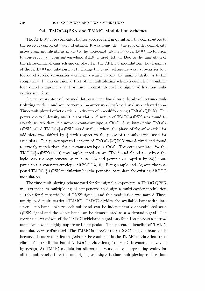
240 9. CONCLUSIONS AND RECOMMENDATIONS
9.4. TMOC-QPSK and TMMC Modulation Schemes
The AltBOC core correlator blocks were studied in detail and the contributors to
the receiver complexity were identi�ed. It was found that the root of the complexity
arises from modi�cations made to the non-constant-envelope AltBOC modulation
to convert it to a constant-envelope AltBOC modulation. Due to the limitation of
the phase-multiplexing scheme employed in the AltBOC modulation, the designers
of the AltBOC modulation had to change the two-level square wave sub-carrier to a
four-level special sub-carrier waveform - which became the main contributor to the
complexity. It was envisioned that other multiplexing schemes could help combine
four signal components and produce a constant-envelope signal with square sub-
carrier waveform.
A new constant-envelope modulation scheme based on a chip-by-chip time- mul-
tiplexing method and square wave sub-carrier was developed, and was referred to as
Time-multiplexed o�set-carrier quadrature-phase-shift-keying (TMOC-QPSK). The
power spectral density and the correlation function of TMOC-QPSK was found to
exactly match that of a non-constant-envelope AltBOC. A variant of the TMOC-
QPSK called TMOC-π4-QPSK was described where the phase of the sub-carrier for
odd slots was shifted by π4with respect to the phase of the sub-carrier used for
even slots. The power spectral density of TMOC-π4-QPSK was derived and found
to exactly match that of a constant-envelope AltBOC. The core correlator for the
TMOC-π4-QPSK(15,10) was implemented on an FPGA and found to reduce the
logic resource requirement by at least 32% and power consumption by 23% com-
pared to the constant-envelope AltBOC(15,10). Being simple and elegant, the pro-
posed TMOC-π4-QPSK modulation has the potential to replace the existing AltBOC
modulation.
The time-multiplexing scheme used for four signal components in TMOC-QPSK
was extended to multiple signal components to design a multi-carrier modulation
suitable for future wideband GNSS signals, and this modulation was named Time-
multiplexed multi-carrier (TMMC). TMMC divides the available bandwidth into
several sub-bands, where each sub-band can be independently demodulated as a
QPSK signal and the whole band can be demodulated as a wideband signal. The
correlation waveform of the TMMC wideband signal was found to possess a narrow
main peak with highly suppressed side-peaks. The potential bene�ts of TMMC
modulation were discussed. The TMMC is superior to AltBOC in a given bandwidth
because: 1) more than four signals can be combined in the TMMC modulation (thus
eliminating the limitation of AltBOC modulation), 2) TMMC is constant envelope
by design, 3) TMMC modulation allows the re-use of same spreading codes for
all the sub-bands since the underlying technique is time-multiplexing rather than

9.5. RECOMMENDATIONS FOR FUTURE WORK 241
phase-multiplexing, 4) TMMC is more robust to interference, multipath and other
frequency selective sources of errors and 5) TMMC is simpler to realise, (i.e. more
�receiver friendly� than AltBOC). Hence TMMC modulation is a better candidate
than AltBOC for the intra-signal modulation discussed in sec. 9.2.3.
9.5. Recommendations for Future Work
9.5.1. Multi-frequency, Multi-GNSS receiver baseband signal process-
ing algorithms. The Galileo E5 AltBOC signal can be considered a super-set of
all the other signals. The research work carried out in this thesis pertaining to the
acquisition and tracking has focussed on the following:
1) Maximising the received signal energy at the output of the correlator (such
as the pre-correlation combination architecture).
2) Combining di�erent signal components to tap the bene�ts o�ered by each
component (such as combining the higher robustness of the wider BPSK-like corre-
lation waveform and higher performance o�ered by the narrow main peak, as in the
hybrid DLL method).
3) Developing simple, but generalised and con�gurable architectures to accom-
modate more than one signal or signal component (such as the hybrid tracking
architecture and the Mixed-radix FFT approach).
The objectives mentioned above can be thought of as the initial design criteria for
the baseband signal processing modules in a multi-frequency, multi-GNSS receiver,
and the methods described in this thesis can be extended.
In addition, speci�c sections that can be improved are:
• A theoretical expression for the threshold can be derived that helps to end
the iterations in the branch elimination method proposed (sec. 4.7) for
extended integration with secondary codes
• A feasibility study of the application of the pre-correlation combination
method (sec. 5.5.3 ) to other GNSS signals could be carried out and its per-
formance evaluated. This is signi�cant because the proposed pre-correlation
combination architecture for the Galileo E5 AltBOC signal o�ers the ad-
vantage of extending the coherent integration duration beyond the data-bit
period
9.5.2. Recon�gurable (hardware / software-de�ned hardware / soft-
ware) multi-GNSS receiver baseband processor. Even if a dedicated Applica-
tion Speci�c Integrated Circuit (ASIC) replaces the FPGA baseband hardware, as a
rule of thumb, and the author's own experience with multiple generations of GPS L1
C/A correlator ASIC design, there will be a best case reduction of the FPGA power
consumption by a factor of 5. In other words, a baseband ASIC will consume about

242 9. CONCLUSIONS AND RECOMMENDATIONS
100 mW for the L1-L5 and about 200-mW for the all civil GPS+Galileo baseband.
This power consumption is very high given that it is only for the baseband hardware
and not for the entire receiver. Finally, if other global and regional satellite naviga-
tion systems (such as GLONASS, Compass, QZSS, IRNSS) are included, then, the
�200 times� estimate of Dempster (2007) mentioned in sec. 2.10.1 would not be far
away. Hence it can be concluded that development of a commercial general purpose
multi-GNSS receiver is still a challenging task.
To address this issue a recon�gurable / time sharing correlator module could
be developed extending the FFT level recon�gurability work carried out for the
acquisition module described in Chapter 7. The author envisages that the following
types of recon�gurability options can be explored:
1) Code generation level recon�gurability - (such work has already commenced
and has been reported in Mumford et.al. (2011).
2) Core correlator or channel level recon�gurability (recon�guring the channel
comprising of carrier generator, code generator, carrier mixer, code mixer and accu-
mulator).
3) Baseband hardware level or signal component level recon�gurability - that is,
a baseband hardware from digitised intermediate frequency bits up to the correlation
values / status/ control passed through a memory mapped interface, is completely
recon�gured for other signals as the need arises.
9.5.3. Performance evaluation of wideband GNSS signals with TMMC
modulation. Chapter 6 suggests that the frequency diversity present in AltBOC
can be used to measure the carrier phases at two points in the frequency spectrum
in order to compensate for the frequency selective code delay distortions midway
between the two points. Using the TMMC modulation, which allows independent
demodulation of all the sub-bands spanning the entire bandwidth in a wideband sig-
nal, more accurate estimation of the frequency selective channel impairments can be
obtained. This needs further investigation. In addition, the potential bene�ts of the
TMMC modulation as explained in sec. 8.7.5 such as continuous wave interference
and DME interference, could be investigated further.
There is an active search for a wideband GNSS signal in the S-band as described
in Mateu et al. (2010). The feasibility of using the TMMC modulation can be anal-
ysed and the advantages with respect to other modulations could also be evaluated.

Bibliography
ABIResearch (2009), Internet. Accessed on 01 Nov 2010.
URL: http://www.abiresearch.com/press/3336
Altera (2004), `FFT 32K Point Design Example v1.0.0'.
URL: http://www.altera.com/support/examples/verilog/ver-�t-32k.html.
Altera (2007), FFT MegaCore Function User Guide Version 7.2, Altera Corpora-
tion.
Altman, F. and Sichak, W. (1956), `A simpli�ed diversity communication system
for beyond-the-horizon links', Communications Systems, IRE Transactions on
4(1), 50 �55.
Antcom (2010), Antcom New GNSS Antennas, Antcom Corporation.
Arthur, B. W. (2009), The Nature of Technology: What it is and how it Evolves,
Free Press, New York.
Avila-Rodriguez, J.-A., Hein, G. W., Wallner, S., Issler, J.-L., Ries, L., Lestarquit,
L., Latour, A. d., Godet, J., Bastide, F., Pratt, T. and Owen, J. (2008), `The
MBOC Modulation: The Final Touch to the Galileo Frequency and Signal Plan',
NAVIGATION: Journal of The Institute of Navigation 55(1), 14�28.
Barker, B., Betz, J. and Clark, J. (2000), Overview of the GPS M code signal, in
`CDROM Proceedings of the ION National Meeting :Navigating into the New
Millennium', Anaheim, Calif, USA.
Barnes, J., Rizos, C., Kanli, M. and A., P. (2006), A Positioning Technology for
Classically Di�cult GNSS Environments from Locata, in `IEEE PLANS', pp. 715�
721.
Bedford, L., Brown, N. and Walford, J. (2009), Leica AR25 White Paper, White
paper, Leica Geosystems.
Betz, J. (Winter 2001-2002), `Binary O�set Carrier Modulations for Radionaviga-
tion', NAVIGATION: Journal of The Institute of Navigation 48, 227�246.
Betz, J. and Goldstein, D. (2002), Candidate designs for an additional civil signal
in GPS spectral bands, Technical report, MITRE, Bedford, Mass, USA.
Bhuiyan, M. Z. H., Lohan, E. S. and M., R. (2007), Peak tracking algorithm for
Galileo-based positioning in multipath fading channels, in `IEEE ICC', Glasgow,
Scotland, UK, pp. 5927�5932.
243

244 Bibliography
Bird, J. (1995), `Calculating the performance of linear and square-law detectors',
Aerospace and Electronic Systems, IEEE Transactions on 31(1), 39 �51.
Bishop, G. J., Klobuchar, J. A. and Doherty, P. H. (1985), `Multipath e�ects on
the determination of absolute ionospheric time delay from GPS signals', Radio
Science 20(3), 388�396.
Borre, K., Akos, D. M., Bertelsen, N., Rinder, P. and Jensen, H. (2007), A Software
De�ned GPS and Galileo Receiver : A Single-Frequency Approach, Birkhauser.
Braasch, M. (1996), GPS Theory and Applications, Vol. 1, AIAA, chapter 14: Mul-
tipath E�ects.
Braasch, M. (2001), Performance comparison of multipath mitigating receiver ar-
chitectures, in `IEEE Aerospace Conf', Vol. 3, Mont, USA, pp. 1309�1315.
Braasch, M. and van Dierendonck, A. (1999), GPS receiver architectures and mea-
surements, in `Proceedings of the IEEE'.
Brown, A. and Mathews, B. (2005), GPS Multipath Mitigation. Using a Three
Dimensional Phased Array, in `ION GNSS', Long Beach, CA.
Burian, A., Lohan, E. and Renfors, M. (2006), BPSK-like Methods for Hybrid-
Search Acquisition of Galileo Signals, in `IEEE ICC'.
Burrus, C. and Selesnick, I. (1995), On programs for prime length �ts and circular
convolution, in `Acoustics, Speech, and Signal Processing, 1995. ICASSP-95., 1995
International Conference on', Vol. 2, pp. 1137 �1140 vol.2.
Butman, S. and Timor, U. (1972), `Interplex�an e�cient multichannel psk/pm
telemetry system', Communications, IEEE Transactions on 20(3), 415 � 419.
Cahn, C., Wang, C., Hegarty, C., Sklar, D., Ma, H. and Betz, J. (2007), `Enhancing
the Future of Civil GPS: Overview of the L1C Signal', Inside GNSS pp. 42�49.
Cameron, A. (2010), `The System: GLONASS Forecast Bright and Plentiful', GPS
World .
URL: http://www.gpsworld.com/gnss-system/the-system-glonass-forecast-bright-
and-plentiful-10580
Chan, A. and Games, R. (1990), `On the linear span of binary sequences obtained
from Q-ary M-sequences, Q odd', Information Theory, IEEE Transactions on
36(3), 548 �552.
Cherubini, G. and Benvenuto, N. (2002), Algorithms for Communications Systems
and their Applications, Wiley Publications.
Cheung, W., Stansell, T. and Fontana, R. D. (2001), `The Modernized L2 Civil
Signal', GPS World .
Corazza, G. E., Palestini, C., Pedone, R. and Villanti, M. (2007), Galileo Primary
Code Acquisition Based on Multi-hypothesis Secondary Code Ambiguity Elimina-
tion, in `Proceedings of the 20th International Technical Meeting of the Satellite
Division of The Institute of Navigation (ION GNSS 2007)', Fort Worth, TX,

Bibliography 245
pp. 2459�2465.
Counselman, C. (1999), Multipath-Rejecting GPS Antennas, in `IEEE', Vol. 87.
Dafesh, P. and Cahn, C. (2009), Phase-Optimized Constant-Envelope Transmission
(POCET) Modulation Method for GNSS Signals, in `Proceedings of the 22nd
International Technical Meeting of The Satellite Division of the Institute of Nav-
igation', Savannah, GA, pp. 2860 � 2866.
De Wilde, W., Sleewaegen, J.-M. and Grnados, S. G. (2007), `Method and Device
for Demodulating Galileo Alternate Binary O�set Carrier (Alt-BOC) signals'.
De Wilde, W., Sleewaegen, J.-M., Simsky, A., Vandewiele, C., Peeters, E., Grauwen,
J. and Boon, F. (2006), Fast signal Acquisition technology for new GPS/Galileo
Receivers, in `IEEE PLANS'.
Dempster, A. G. (2006), `Correlators for L2C: Some Considerations', Inside GNSS
pp. 32�37.
Dempster, A. G. (2007), Satellite navigation: New signals, new challenges, in
`Circuits and Systems, 2007. ISCAS 2007. IEEE International Symposium on',
pp. 1725 �1728.
Dempster, A. G. and Rizos, C. (2009), Implications of a System of Systems Receiver,
in `Surveying & Spatial Sciences Institute Biennial International Conference', Ade-
laide, Australia.
Dierendonck, A. J. V. (1996), Global Positioning System: Theory and Applications,
Vol. 1, American Institute of Aeronautics and Astronautics, chapter 8 GPS Re-
ceivers, pp. 329�407.
Diggelen, F.-v. (2009), A-GPS Assisted GPS, GNSS and SBAS, Artech House.
Djebouri, D., A, D. and M, D. (2006), `Robust GPS Satellite Signal Acquisition
Using Lifting Wavelet Transform', Radio Engineering 15(1).
Dovis, F., Mulassano, P. and Margaria, D. (2007), Multiresolution Acquisition En-
gine Tailored to the Galileo AltBOC Signals, in `ION GNSS'.
Eissfeller, B., Amer, G., Kropp, V. and Sanroma, D. (2007), Performance of GPS,
GLONASS and Galileo, in `Photogrammetric Week 07', Wichmann, Stuttgart.
Ettus, M. (2010), The USRP Product Family, Ettus Research.
EuropeanCommission (Internet). Accessed 01 Nov 2010.
URL: http://ec.europa.eu/enterprise/policies/satnav/galileo/programme/index_en.htm
Falcone, M., Erhard, P. and Hein, G. (2006), Understanding GPS: Principles and
Applicatio, 2 edn, Artech House, chapter 10: Galileo.
Fan, T., Lin, V., Wang, G. and Dafesh, P. (2008), Study of Signal Combining
Methodologies for Future GPS Flexible Navigation Payload, in `Proceedings of
IEEE/ION PLANS', Monterey, CA, pp. 1079 � 1089.
Fante, R. L. (2003), Unambiguous tracker for GPS Binary O�set Carrier signals,
in `ION 59th AM / CIGTF 22nd guidance test symposium', Albuquerque New

246 Bibliography
Mexico.
Feng, Y. and Rizos, C. (2005), Three Carrier Approaches for Future Global, Regional
and Local GNSS Positioning Services: Concepts and Performance Perspectives,
in `ION GNSS', Long Beach, CA, pp. 2277�2787.
Fine, P. and Wilson, W. (1999), Tracking algorithm for GPS o�set carrier signals,
in `ION NTM'.
Fischer, S., Guerin, A. and Berberich, S. (2004), Acquisition concepts for galileo
boc(2,2) signals in consideration of hardware limitations, in `Vehicular Technology
Conference, 2004. VTC 2004-Spring. 2004 IEEE 59th', Vol. 5, pp. 2852 � 2856
Vol.5.
Fontana, R. D., Cheung, W., Novak, P. M. and Stansell, T. A. (2001), The New L2
Civil Signal, in `Proceedings of the 14th International Technical Meeting of the
Satellite Division of The Institute of Navigation', Salt Lake City, UT, pp. 617�631.
Gao, G., Datta-Barua, S., Walter, T. and Enge, P. (2007), Ionosphere E�ects for
Wideband GNSS Signals, in `ION NTM'.
Garin, L. J. (2005), The Shaping Correlator, Novel Multipath Mitigation Technique
Applicable to GALILEO BOC(1,1) Modulation Waveforms in High Volume. Mar-
kets, in `ENC GNSS', Munich.
Garin, L. and Rousseau, J. (1997), Enhanced Strobe Correlator Multipath Rejection
for Code and Carrier, in `ION GPS', Kansas City, Missouri, pp. 559�568.
Gerein, N. (2007), `Hardware Architectures for Processing Galileo Binary O�set
Carrier Signals'.
GIOVEABICD (2008), `GIOVE-A+B Navigation Signal-In-Space Interface Control
Document'.
Giunta, G. and Benedetto, F. (2007), `Spread-spectrum code acquisition in the
presence of cell correlation', Communications, IEEE Transactions on 55(2), 257
�261.
GLOANSSICD (n.d.), `GLONASS Interface Control Document (Rev. 1995)'. Eng-
lish Translation of Russian Document.
Goldsmith, A. (2005), Wireless Communications, Cambridge University Press.
GPSGALPERF (2010), COMBINED PERFORMANCES FOR OPEN
GPS/GALILEO RECEIVERS, Combsps, EU-US Cooperation on Satellite
Navigation, Working Group C.
GPSJPO (2000), Global Positioning System (GPS) Modernization, Technical report,
U.S. Air Force,GPS Joint Program O�ce,Los Angeles AFB.
GPSSPS (2001), `Global Positioning System Standard Positioning Service Perfor-
mance Standard'.
GPSSPS (2008), `Global Positioning System Standard Positioning Service Perfor-
mance Standard'.

Bibliography 247
GSA (2009), `Gnss market monitor', Internet. Accessed 01 Nov 2010.
URL: http://www.egnos-portal.eu/index.cfm?objectid=65117DB1-14B7-11DF-
93B6005056861A4B
Haber, F. and Noorchashm, M. (1974), `Negatively Correlated Branches in Fre-
quency Diversity Systems to Overcome Multipath Fading', IEEE Transactions on
Communications 22(2), 180�190.
Hegarty, C. (1999), Evaluation of the Proposed Signal Structure for the New Civil
GPS Signal at 1176.45 MHz, Working Note WN99W0000034, MITRE Corpora-
tion.
Hegarty, C. (2006), Optimal and Near Optimal Detectors for Acquisition of the GPS
L5 Signal, in `Proceedings of the National Technical Meeting of The Institute of
Navigation', Monterey, CA, pp. 717�725.
Hegarty, C. (2009), Analytical Model for GNSS Receiver Implementation Losses, in
`U.S. Institute of Navigation International Technical Meeting, ION GNSS'.
Hegarty, C., Betz, J. W. and Saidi, A. (2004), Binary Coded Symbol Modulations
for GNSS, in `Proceedings of the Annual Meeting of The Institute of Navigation',
Dayton, OH, pp. 56�64.
Heiries, V., Roviras, D., Ries, L. and Calmettes, V. (2004), Analysis of Non Am-
biguous BOC Signal Acquisition Performance, in `ION GNSS'.
Ho�mann-Wellenhof, B., Lichtenegger, H. and Wasle, E. (2008), GNSS : Global
Navigation Satellite Systems : GPS, GLONASS, Galileo & more, SpringerWein-
NewYork.
Holmes, J. (1982), Coherent Spread Spectrum Systems, John Wiley & Sons.
Holmes, J. (2007), Spread Spectrum Systems For GNSS and Wireless Communica-
tion Systems, Artech House.
Hu, J. and Beaulieu, N. (2005a), `Accurate closed-form approximations to Ricean
sum distributions and densities', Communications Letters, IEEE 9(2), 133 � 135.
Hu, J. and Beaulieu, N. (2005b), `Accurate simple closed-form approximations
to Rayleigh sum distributions and densities', Communications Letters, IEEE
9(2), 109 � 111.
Irsigler, M. and Eissfeller, B. (2003), Comparison of Multipath Mitigation Tech-
niques with Consideration of Future Signal Structures, in `ION GPS/GNSS',
Portland, OR.
ISGPS200E (2010), `Navstar GPS Space Segment/Navigation User Interfaces IN-
TERFACE SPECIFICATION'.
URL: http://www.gps.gov/technical/icwg/IS-GPS-200E.pdf
ISGPS705 (2010), `Navstar GPS Space Segment / User Segment L5 Interfaces IN-
TERFACE SPECIFICATION'.
URL: http://www.gps.gov/technical/icwg/IS-GPS-705A.pdf
248 Bibliography
ISGPS800 (2010), `Navstar GPS Space Segment/User Segment L1C Interface IN-
TERFACE SPECIFICATION'.
URL: http://www.gps.gov/technical/icwg/IS-GPS-800A.pdf
Issler, J.-L., Ries, L., Lestarquit, L., Nouvel, O. and Jeandel, Q. (2003), Spectral
Measurement of GNSS Satellite Signals Need for Wide Transmitted Bands, in
`ION GPS/GNSS', pp. 445�460.
Jacobson, L. (2007), GNSS Markets and Applications, Artech House, chapter 6
Future GNSS Markets, pp. 95�114.
Kaplan, E. D. and Hegarty, C. J., eds (2006), Understanding GPS: Principles and
Applications, Artech House.
Kelly, J. M. and Braasch, M. S. (1999), Mitigation of GPS multipath via exploitation
of signal dynamics, in `ION Annual Meeting', Cambridge, MA, pp. 619�624.
Kelly, J. M., Braasch, M. S. and M, D. (2003), `Characterization of the e�ects of
high multipath phase rates in GPS', GPS Solutions 7(1).
Kunysz, W. (2003), A Three Dimensional Choke Ring. Ground Plane Antenna, in
`ION GNSS', Portland, OR, pp. 1883�1888.
Lestarquit, L., Artaud, G. and Issler, J.-L. (2008), AltBOC for Dummies or Ev-
erything You Always Wanted To Know About AltBOC, in `Proceedings of the
21st International Technical Meeting of the Satellite Division of The Institute of
Navigation', Savannah, GA, USA, pp. 961�970.
Lohan, E., Lakhzouri, A. and Renfors, M. (2006), `Complex double-binary-o�set-
carrier modulation for a unitary characterisation of Galileo and GPS signals',
Radar, Sonar and Navigation, IEE Proceedings - 153(5), 403�408.
Lu, M. (2010), Status of compass development, in `Stanford PNT Symposium'.
Lyusin (1998), Fast Acquisition by Matched Filter Technique for GPS/GLONASS
Receivers, in `Institute of Navigation: Satellite Division-International technical
meeting, Proceedings of ION GPS'.
Malik, S. A., Shivaramaiah, N. C. and Dempster, A. G. (2009a), FPGA-based GNSS
Search Engine using Parallel Techniques in the Time-Domain, in `IGNSS Symp',
Gold Coast, Australia.
Malik, S. A., Shivaramaiah, N. C. and Dempster, A. G. (2009b), Search engine trade-
o�s in FPGA-based GNSS receiver designs, in `European Navigation Conference
ENC-GNSS', Naples, Italy.
Marcum, J. (1960), `A statistical theory of target detection by pulsed radar: Math-
ematical appendix', Information Theory, IRE Transactions on 6(2), 145 �267.
Margaria, D. and Dovis, F. (2008), `An Innovative Data Demodulation Technique
for Galileo AltBOC Receivers', Journal of Global Positioning System 6(1), 89�96.
Martin, N., Leblond, V., Guilliotel, G. and Heiries, V. (2003), BOC(x,y) Signal
Acquisition Techniques and Performances, in `ION GPS/GNSS'.

Bibliography 249
Mateu, I., Paonni, M., Issler, J.-L. and Hein, G. W. (2010), `A search for spectrum:
GNSS signals in S-band, Part II', Inside GNSS pp. 46�53.
Mattos, P. (2006), The Implications of Simultaneous Processing of the Galileo L1b/c
signals, in `ION-GNSS', Fortworth, Texas, pp. 1861�1865.
McDonough, R. N. and Whalen, A. D. (1995), Detection of Signals in Noise, second
edn, Academic Press.
McGraw, G. A. (2010), GNSS Receiver Panel Discussion: Modernized GNSS Re-
ceiver System Issues, in `ION GNSS', Portland, OR.
McGraw, G. A. and Braasch, M. (1999), GNSS Multipath Mitigation Using Gated
and High Resolution Correlator Concepts, in `ION NTM', San Diego, CA, pp. 333�
342.
Moelker, D. (1997), Multiple Antennas for Advanced GNSS Multipath Mitigation
and Multipath Direction Finding, in `ION GPS', Kansas City, pp. 541�550.
Namgoong, W., Reader, S. and Meng, T. (2000), `An all-digital low-power IF GPS
synchronizer', Solid-State Circuits, IEEE Journal of 35(6), 856�864.
Nedic, S. (2009), On GPS Signal Multipath Modeling in Dynamic Environments, in
`Aerospace Conference'.
NovAtel (2010), GPS-704X Antenna Design and Performance, Technical report,
NovAtel Inc.
Nuñes, F., F., S. and J., L. (2004), Multipath Mitigation Technique for BOC signals
Using Gating Functions, in `NAVITEC Workshop', Noordwijk, NL.
Nunes, F., Sousa, F. and Leitao, J. (2007), `Gating functions for Multipath mitiga-
tion in BOC Signals', IEEE Transactions on Aerospace and Electronic Systems
43(3).
Oleynik, E. (2010), GLObal Navigation Satellite System(GLONASS) , Central Re-
search Institute of Machine Building, PNT Center, Chisinau, Moldova.
Oppenheim, A. V. and Schafer, R. W. (1998), Discrete-Time Signal Processing, 2
edn, Prentice Hall.
Orban, D. and Moernaut, G. (2009), `GNSS Antennas: An Introduction to Band-
width, Gain Pattern, Polarization and All That', GPS World .
OSSISICD (2010), `European gnss (galileo) open service signal in space interface
control document'.
Otoshi, T. (1993a), `The E�ect of Multipath on the Antenna Time Delays', IEEE
Antenna and Propagation Magazine 35(5), 28�36.
Otoshi, T. (1993b), `The e�ects of multipath on the measurement of antenna time
delays', Antennas and Propagation Magazine, IEEE 35(5), 28�36.
Pany, T., M., I. and B., E. (2005), S-curve shaping: a new method for optimum dis-
criminator based code multi-path mitigation, in `ION GPS/GNSS', Long Beach,
CA, pp. 2139�2154.

250 Bibliography
Parkinson, B. and Spilker, J., eds (1995), Global Positioning System: Theory and
Applications, American Institute of Aeronautics and Astronautics.
Peterson, R. L., Roger, Z. E. and Borth, D. E. (1995), Introduction To Spread
Spectrum Communications, Prentice Hall.
Polydoros, A. and Weber, C. (1984a), `A Uni�ed Approach to Serial Search Spread-
Spectrum Code Acquisition�Part I: General Theory', Communications, IEEE
Transactions on [legacy, pre - 1988] 32(5), 542�549.
Polydoros, A. and Weber, C. (1984b), `A Uni�ed Approach to Serial Search Spread-
Spectrum Code Acquisition�Part II: A Matched-Filter Receiver', Communica-
tions, IEEE Transactions on [legacy, pre - 1988] 32(5), 550�560.
Pratt, A. and Owen, J. (2005), Signal Multiplex Techniques in Satellite Channel
Availability Possible Applications to Galileo, in `Proceedings of the 18th Interna-
tional Technical Meeting of the Satellite Division of The Institute of Navigation',
Long Beach, California, USA.
Proakis, J. G. (2000), Digital Communications, 4 edn, Mcgraw-hill Professional.
Proakis, J. G. and Manolakis, D. (1995), Digital Signal Processing, Principles, Al-
gorithms, and Applications, Prentice Hall.
Pun, M., Morelli, M. and Kuo, C.-C. J. (2007), Multi-Carrier Techniques for Broad-
band Wireless Communications: A Signal Processing Perspective, Imperial College
Press.
Qaisar, S. U., Shivaramaiah, N. C. and Dempster, A. G. (2008), Exploiting the
spectrum envelope for GPS-L2C signal acquisition, in `European Navigation Con-
ference, ENC-GNSS', Toulouse, France.
Qaisar, S. U., Shivaramaiah, N. C., Dempster, A. G. and Rizos, C. (2008), Filtering
IF samples to reduce computational load of frequency domain acquisition in GNSS
receivers, in `21st Int. Tech. Meeting of the Satellite Division of the U.S. Inst. of
Navigation ION-GNSS', Savannah, Georgia, pp. 236�243.
Rappaport, T. S. (2002), Wireless Communications: Principles and Practice, 2 edn,
Prentice Hall.
Ray, J. (2000), Mitigation of GPS Code and Carrier Phase Multipath E�ects Using
a Multi-Antenna System, PhD thesis, University of Calgary.
Ray, J. K., Cannon, M. and P., F. (1999), Code Range and Carrier Phase Multi-
path Mitigation using SNR, Range and Phase Measurements in a Multi-Antenna
System, in `ION GPS', Nashville.
Rebeyrol, E. (2007), Galileo Signals and Payload Optimization, PhD thesis, Ecole
Nationale Supérieure des. Télécommunications.
Rebeyrol, E., Macabiau, C., Lestarquit, L., Ries, L., Issler, J.-L., Boucheret, M.-
L. and Bousquet, M. (2005), BOC Power Spectrum Densities, in `ION National
Technical Meeting'.

Bibliography 251
Rebeyrol, E., Macabiau, C., Ries, L., Issler, J.-L., Bousquet, M. and Boucheret,
M.-L. (2006), Interplex Modulation for Navigation Systems at the L1 Band, in
`Proceedings of the 2006 National Technical Meeting of The Institute of Naviga-
tion', Monterey, CA, pp. 100�111.
Ries, L., Legrand, F., Lestarquit, L., Vigneau, W. and Issler, J.-L. (2003), Tracking
and Multipath Performance Assessments of BOC Signals Using a Bit-Level Signal
Processing Simulator, in `ION GPS/GNSS', Portland, OR, USA, pp. 1996�2010.
Ries, L., Lestarquit, L., Armengou-Miret, E., Legrand, F., Vigneau, W., Bourga,
C., Erhard, P. and Issler, J.-L. (2002), A Software Simulation Tool for GNSS2
BOC Signals, in `ION GPS', Portland, OR, USA, pp. 2225�2239.
Rodríguez, J.-n. v. (2008), On Generalized Signal Waveforms for Satellite Naviga-
tion, PhD thesis, Faculty of Aerospace Engineering, Universität der Bundeswehr
München.
Sajabi, C., Chen, C.-I., Lin, D. and Tsui, J. (2006), Fpga frequency domain based
gps coarse acquisition processor using �t, in `Instrumentation and Measurement
Technology Conference, 2006. IMTC 2006. Proceedings of the IEEE', pp. 2353
�2358.
Sarwate, D. and Pursley, M. (1980), `Crosscorrelation properties of pseudorandom
and related sequences', Proceedings of the IEEE 68(5), 593�619.
Septentrio (2006), GeNeRx1 Data sheet, Septentrio.
Seybold (2005), Introduction to RF Propagation, Wiley Interscience.
Sheen, W.-H., Tzeng, J.-K. and Tzou, C.-K. (1999), `E�ects of cell correlations in a
matched-�lter pn code acquisition for direct-sequence spread-spectrum systems',
Vehicular Technology, IEEE Transactions on 48(3), 724 �732.
Shivaramaiah, N. C. (2004), A Fast Acquisition Hardware GPS Correlator, Master's
thesis, Center for Electronics Design and Technology, Indian Institute of Science,
Bangalore, India.
Shivaramaiah, N. C. (2009), Code phase multipath mitigation by exploiting the
frequency diversity in Galileo E5 AltBOC, in `22nd Int. Tech. Meeting of the
Satellite Division of the U.S. Inst. of Navigation ION GNSS', Savannah, Georgia.
Shivaramaiah, N. C. and Dempster, A. G. (2008a), An Analysis of Galileo E5 Sig-
nal Acquisition Strategies, in `European Navigation Conference, ENC-GNSS',
Toulouse, France.
Shivaramaiah, N. C. and Dempster, A. G. (2008b), An unambiguous detector archi-
tecture for galileo es signal acquisition, in `Signals, Systems and Computers, 2008
42nd Asilomar Conference on', pp. 2076 �2080.
Shivaramaiah, N. C. and Dempster, A. G. (2009a), A novel extended tracking range
DLL for AltBOC signals, in `Vehicular Technology Conference, 2009. VTC Fall
2009. IEEE 70th'.

252 Bibliography
Shivaramaiah, N. C. and Dempster, A. G. (2009b), `Processing complex-modulated
signals involving spreading code and subcarrier in ranging systems'.
Shivaramaiah, N. C. and Dempster, A. G. (2010a), Group delay compensation in
altboc receivers to mitigate the e�ect of frequency selective propagation delay
distortions, in `Position Location and Navigation Symposium (PLANS), 2010
IEEE/ION', pp. 227 �235.
Shivaramaiah, N. C. and Dempster, A. G. (2010b), On the baseband hardware
complexity of modernized GNSS receivers, pp. 3565 �3568.
Shivaramaiah, N. C., Dempster, A. G. and Rizos, C. (2008), Exploiting the sec-
ondary codes to improve signal acquisition performance in Galileo receivers, in
`21st Int. Tech. Meeting of the Satellite Division of the U.S. Inst. of Navigation
ION-GNSS', Savannah, Georgia, pp. 1497�1506.
Shivaramaiah, N. C., Dempster, A. G. and Rizos, C. (2009a), A hybrid tracking loop
architecture for Galileo E5 signal, in `European Navigation Conference', Naples,
Italy.
Shivaramaiah, N. C., Dempster, A. G. and Rizos, C. (2009b), `Application of Prime-
factor and Mixed-radix FFT Algorithms in Multi-band GNSS Receivers', Journal
of GPS 8, 174�186.
Shivaramaiah, N. C., Dempster, A. G. and Rizos, C. (2010), `Time-Multiplexed-
O�set-Carrier Modulations for GNSS', IEEE Trans. AES (under review) .
Shivaramaiah, N. C., Dempster, A. G. and Rizos, C. (2011), On E�cient Wideband
GNSS Signal Design, in `To appear in the proceedings of ION ITM 2011', San
Diego, CA.
Shnidman, D. A. (1989), `The Calculation of the Probability of Detection and
the Generalized Marcum Q Function', IEEE Transaction on Information The-
ory 35(2).
Simon, M. (2002), Probability Distributions Involving Gaussian Random Variables,
Springer.
Sleewaegen, J.-M., De Wilde, W. and Hollreiser, M. (2004), Galileo AltBOC Re-
ceiver, in `ENC GNSS'.
Smith, W. (1995), Handbook of Real-Time Fast Fourier Transforms : Algorithms to
Product Testing, John Wiley & Sons.
Soellner, M. and Erhard, P. (2003), Comparison of AWGN Code Tracking Accuracy
for Alternative-BOC, Complex-LOC and Complex-BOC Modulation Options in
Galileo E5-Band, in `ENC GNSS'.
Sorensen, H., Heideman, M. and Burrus, C. (1986), `On computing the split-radix
�t', Acoustics, Speech and Signal Processing, IEEE Transactions on 34(1), 152 �
156.

Bibliography 253
Spilker, J. (1977), Digital Communications by Satellite, Prentice-Hall, Englewood
Cli�s, NJ.
Spilker, J. J. J. (2010), Generalized Binary Coded Symbol Modulation Theoreti-
cal Performance with Multipath and Noise, in `Proceedings of the International
Technical Meeting of The Institute of Navigation', San Diego, CA, pp. 750�764.
Stansell, T. (Online), `Update on GPS L1C Signal Modernization (Presentation)'.
URL: http://www.spirentfederal.com/documents/Stansell-L1C-Update-v03.pdf
Starzyk, J. and Zhu, Z. (2001), Averaging correlation for c/a code acquisition and
tracking in frequency domain, in `Circuits and Systems, 2001. MWSCAS 2001.
Proceedings of the 44th IEEE 2001 Midwest Symposium on', Vol. 2, pp. 905 �908
vol.2.
Ta, T. H., Shivaramaiah, N. C., Dempster, A. G. and Lo Presti, L. (accepted for
publication), `Signi�cance of Cell Correlations in GNSS Matched Filter Acquisi-
tion Engines', IEEE Transactions on Aerospace and Electronic Systems .
TheWhiteHouse (2000), `Statement By The President Regarding The United States
Decision To Stop Degrading Global Positioning System Accuracy'.
URL: http://www.ngs.woc.noaa.gov/FGCS/info/sans_SA/docs/statement.html
Townsend, B. and Fenton, P. (1995), Ll Carrier Phase Multipath Error Reduction
Using MEDLL Technology, in `ION GPS', Palm Springs, CA.
Tran, M. (2004), `Performance Evaluation of the New GPS L5 and L2 Civil (L2C)
Signals', Navigation 51(3), 199�212.
Tran, M.and Hegarty, C. (2002), Receiver Algorithms for the New Civil GPS Signals,
in `ION NTM', San Diego, California, pp. 778�789.
Tse, D. and Viswanath, P. (2005), Fundamentals of Wireless Communication, Cam-
bridge University Press.
TychoUSNO (Interneta).
URL: ftp://tycho.usno.navy.mil/pub/gps/gpsb2.txt
TychoUSNO (Internetb), `USNO NAVSTAR Global Positioning System', Internet.
URL: http://tycho.usno.navy.mil/gpsinfo.html
USCG (Internet), `General information on GPS', Internet.
URL: http://www.navcen.uscg.gov/?pageName=GPS
van den Berg, A., Willems, T., Pye, G., de Wilde, W., Morgan-Owen, R., de Mateo,
J., Scara�a, S. and Hollreiser, M. (2010), `Galileo Test User Receiver', GPS World
.
Van Nee, R. and Coenen, A. (1991), `New Fast GPS code-acquisition technique
using FFT', Electronics Letters 27(2), 158�160.
Veitsel, V., Zhdanov, A. and Zhodzishsky, M. (1998), `The mitigation of multipath
errors by strobe correlators in GPS/GLONASS receivers', GPS Solutions 2(2), 38�
45.

254 Bibliography
Viterbi, A. J. and Omura, J. K. (1979), Principles of Digital Communication and
Coding, 1st edn, McGraw-Hill, Inc., New York, NY, USA.
WAASSPS (2008), `Global positioning system wide area augmentation system
(waas) performance standard'.
Ward, P., Betz, J. and Hegarty, C. (2006), Understanding GPS: Principles and Ap-
plications, 2 edn, Artech House, chapter Interference, Multipath and Scintillation.
Watson, G. (2008), `Ionosphere Delay Measurement Using Carrier Phase'.
Wilde, A. (1995), Extended tracking range delay-locked loop, in `International Con-
ference on Communications ICC', pp. 1051�1054.
Wilde, A. (1998a), `Correlation branch selection for extended tracking range delay-
locked loops', European Transactions on Telecommunications 9(1), 57�64.
Wilde, A. (1998b), `The generalized delay-locked loop', Wireless Personal Commu-
nications 8(2), 113�130.
Won, J.-H. and Lee, J.-S. (2005), `A Note on the Group De and Phase Advance
Phenomenon Associated with GPS Signal Progpagation through the Ionosphere',
Navigation: Journal of the Institute of Navigation 52, 95�97.
Yang, C. (2001), FFT Acquisition of Periodic, Aperiodic, Punctured and Overlaid
Code Sequences in GPS, in `ION GPS', Salt Lake City, Utah.
Yang, C., Hegarty, C. and Tran, M. (2004), Acquisition of the GPS L5 Signal Us-
ing Coherent Combining of I5 and Q5, in `ION-GNSS', Long Beach, California,
pp. 2184�2195.
Yoon, S., Song, I., Kim, S. Y. and Park, S. R. (2000), `A DS-CDMA code acquisition
scheme robust to residual code phase o�set variation', Vehicular Technology, IEEE
Transactions on 49(6), 2405�2418.
Yun, S., Chang, D. and Yom, I. (2008), Wideband Receive Antennas of Sensor Sta-
tions for GPS/Galileo Satellite, in `Advanced Satellite Mobile Systems', pp. 210�
212.
Zarlink (1999), GPS Receiver Hardware Design Application Note AN4855, 2.0 edn,
Zarlink Semiconductor.
Zarlink (2001), GPS 12 channel correlator, issue 3.2 edn, Zarlink Semiconductor.
Zhuang and Tranquilla (1995), `E�ects of multipath and antenna on GPS observ-
ables', IEE Radar Sonar and Navigation 142(5), 267�275.

APPENDIX A
Fundamentals of AltLOC and AltBOC-NCE modulation
This appendix describes the Alternate Linear O�set Carrier (AltLOC) and the
non-constant envelope Alternate Binary O�set Carrier (AltBOC-NCE) with a slightly
di�erent treatment to that available in Lestarquit et al. (2008).
The baseband signal - AltLOC modulation. The baseband signal is a com-
plex signal which comprises four codes modulated onto the orthogonal components of
a complex subcarrier. In order to understand the basic concept of AltBOC modula-
tion, it is useful �rst to understand the AltLOC equivalent, because the sub-carriers
in AltLOC modulation are pure tones and hence simpler to deal with than AltBOC.
The baseband signal in AltLOC can be expressed as (CAL = CosAltLOC)
sCAL(t) = sb(t) ejωsct + sa(t) e
−jωsct
= (sbI(t) + jsbQ(t)) ejωsct + (saI(t) + jsaQ(t)) e−jωsct
= sbI(t) ejωsct + saI(t) e
−jωsct + sbQ(t) ej(ωsct+π2
) (A.1)
+saQ(t) e−j(ωsct−π2
)
The modulated signal can thus be represented as
SCAL(t) =√
2PT<[(sbI(t) ejωsct + saI(t) e
−jωsct (A.2)
+ sbQ(t) ej(ωsct+π2
) + saQ(t) e−j(ωsct−π2
)) ejωct]
=√
2PT<[sbI(t) ej(ωc+ωsc)t + saI(t) e
j(ωc−ωsc)t
+ sbQ(t) ej((ωc+ωsc)t+π2
) + saQ(t) ej((ωc−ωsc)t+π2
)]
= sbI(t) cos((ωc + ωsc)t) + saI(t) cos((ωc − ωsc)t)− sbQ(t) sin((ωc + ωsc)t)
− saQ(t) sin((ωc − ωsc)t) (A.3)
= sbI(t) cos(ωbt)− sbQ(t) sin(ωbt) + saI(t) cos(ωat)− saQ(t) sin(ωat)
(A.4)
where ωb = (ωc + ωsc) and ωa = (ωc − ωsc) are the E5b and E5a centre frequencies
(see Table (1.1)) respectively.
From the above equation it can be inferred that the transmitted signal spectrum
is real and has two lobes centred at ωb and ωa. A pictorial representation of this
equation is shown in Fig. A.1. Also note (through (A.3)) how the spreading code
(with data) phase modulates the sum and di�erence carriers.
255

256 A. FUNDAMENTALS OF ALTLOC AND ALTBOC-NCE MODULATION
ω-ωc
-ωc-ω
s
-ωc+ω s
E5a
-I
E5b
-I
E5a-QE5b-Q
ω c
ω c-ωs
ω c+ω s
E5a
-I
E5b
-I
E5a-QE5b-Q
0
Figure A.1. spectrum of the cosine-AltLOC
Note that because the baseband complex signal is formulated by addition of
two exponential functions, this modulation is in fact Cosine-AltLOC (CAL). If the
baseband complex signal is formulated by the di�erence of two exponential functions,
then the modulation will be SineAltLOC. The equation for the Sine-AltLOC (SAL)
is then
sSAL(t) = −j ·(sb(t) e
jωsct − sa(t) e−jωsct)
= e−jπ2 ·(sb(t) e
jωsct − sa(t) e−jωsct)
(A.5)
= (sbI(t) + jsbQ(t)) ej(ωsct−π2
) − (saI(t) + jsaQ(t)) e−j(ωsct+π2
)
= sbI(t) ej(ωsct−π2 ) − saI(t) e−j(ωsct+
π2
) (A.6)
+sbQ(t) ejωsct − saQ(t) e−jωsct
The corresponding transmitted signal becomes
SSAL(t) =√
2PT<[(sbI(t) ej(ωsct−π2 ) − saI(t) e−j(ωsct+
π2
) (A.7)
+ sbQ(t) ejωsct − saQ(t) e−jωsct) ejωct]
=√
2PT<[sbI(t) ej((ωc+ωsc)t−π2 ) − saI(t) ej((ωc−ωsc)t−
π2
)
+ sbQ(t) ej(ωc+ωsc)t − saQ(t) ej(ωc−ωsc)t]
= sbI(t) sin((ωc + ωsc)t)− saI(t) sin((ωc − ωsc)t) + sbQ(t) cos((ωc + ωsc)t)
− saQ(t) cos((ωc − ωsc)t) (A.8)
= sbI(t) sin(ωbt) + sbQ(t) cos(ωbt)− saI(t) sin(ωat)− saQ(t) cos(ωat)
(A.9)
The spectrum representation of SAL is shown in Fig. A.2. The spectrum is
similar to that of the CAL except that the baseband components occupy di�erent
phases of the carrier.
The baseband signal - AltBOC-NCE modulation. The subcarrier in the
case of AltBOC-NCE modulation is a complex square wave, unlike the pure tone
used for AltLOC. Using the square wave instead of a pure tone greatly reduces
the burden on the subcarrier generation hardware (or software). Mathematically,
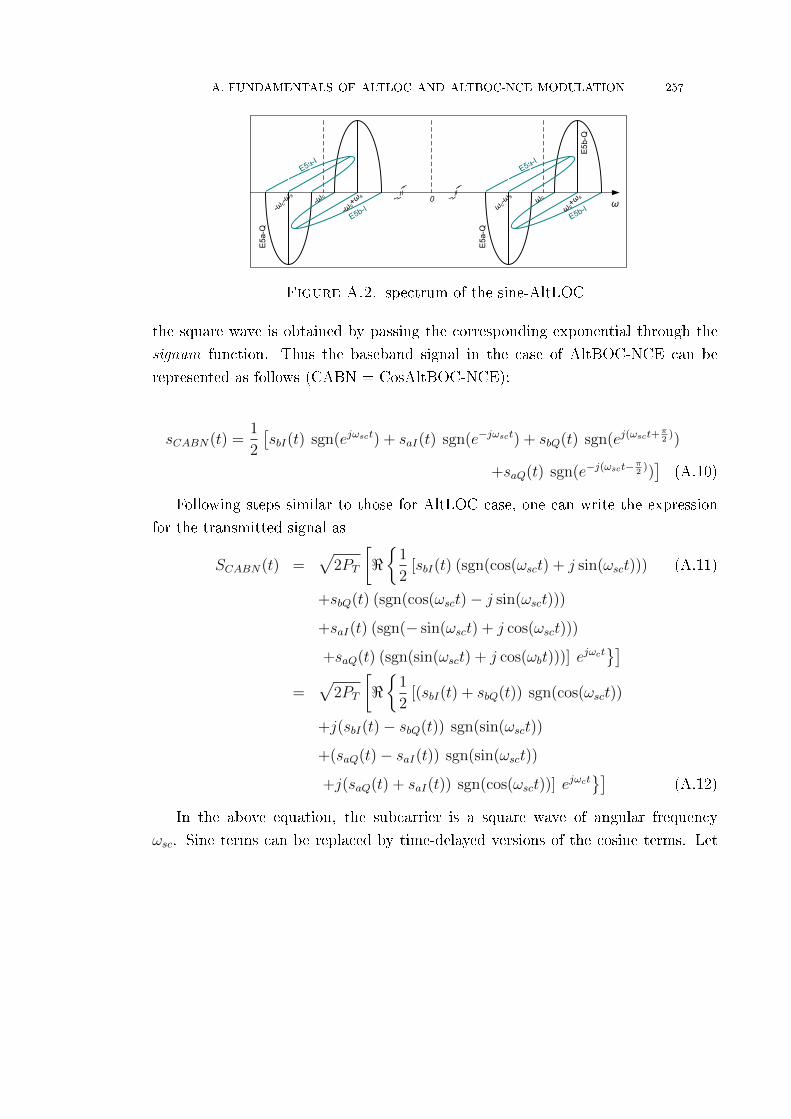
A. FUNDAMENTALS OF ALTLOC AND ALTBOC-NCE MODULATION 257
ω
E5b
-Q
0 ω c
ω c-ωs
ω c+ω s
E5a
-Q
E5a-I
E5b-I-ω
c
-ωc-ω
s
-ωc+ω s
E5a
-Q
E5a-I
E5b-I
Figure A.2. spectrum of the sine-AltLOC
the square wave is obtained by passing the corresponding exponential through the
signum function. Thus the baseband signal in the case of AltBOC-NCE can be
represented as follows (CABN = CosAltBOC-NCE):
sCABN(t) =1
2
[sbI(t) sgn(ejωsct) + saI(t) sgn(e−jωsct) + sbQ(t) sgn(ej(ωsct+
π2
))
+saQ(t) sgn(e−j(ωsct−π2
))]
(A.10)
Following steps similar to those for AltLOC case, one can write the expression
for the transmitted signal as
SCABN(t) =√
2PT
[<{
1
2[sbI(t) (sgn(cos(ωsct) + j sin(ωsct))) (A.11)
+sbQ(t) (sgn(cos(ωsct)− j sin(ωsct)))
+saI(t) (sgn(− sin(ωsct) + j cos(ωsct)))
+saQ(t) (sgn(sin(ωsct) + j cos(ωbt)))] ejωct}]
=√
2PT
[<{
1
2[(sbI(t) + sbQ(t)) sgn(cos(ωsct))
+j(sbI(t)− sbQ(t)) sgn(sin(ωsct))
+(saQ(t)− saI(t)) sgn(sin(ωsct))
+j(saQ(t) + saI(t)) sgn(cos(ωsct))] ejωct}]
(A.12)
In the above equation, the subcarrier is a square wave of angular frequency
ωsc. Sine terms can be replaced by time-delayed versions of the cosine terms. Let

258 A. FUNDAMENTALS OF ALTLOC AND ALTBOC-NCE MODULATION
Tsc = 1fsc
be the period of the square wave. Then (A.12) can be written as
SCABN(t) =√
2PT
[<{
1
2[(sbI(t) + sbQ(t)) sgn(cos(ωsct))
+ j(sbI(t)− sbQ(t)) sgn(cos(ωsct− Tsc4
))
+ (saQ(t)− saI(t)) sgn(cos(ωsct− Tsc4
))
+j(saQ(t) + saI(t)) sgn(cos(ωsct))] ejωct}]
(A.13)
=√
2PT
[<{
1
2
[(sbI(t) + sbQ(t)) sc(t) + j(sbI(t)− sbQ(t)) sc(t− Tsc
4)
+ (saQ(t)− saI(t)) sc(t− Tsc4
)) + j(saQ(t) + saI(t)) sc(t)]ejωct
}](A.14)
where sc(t) = sgn(cos(ωsct)) is the subcarrier component. As an example, a single
cycle of the subcarrier waveform for AltBOC-NCE(15,10) which has fsc=15.345 MHz
and the code frequency fco=10.23 MHz is shown in Fig. A.3.
0 0.1 0.2 0.3 0.4 0.5 0.6 0.7 0.8 0.9 1−2
−1.5
−1
−0.5
0
0.5
1
1.5
2
Am
plitu
de
tTsc
sc(t)
sc(t − Tsc
4 )
Figure A.3. subcarrier in AltBOC-NCE
Note that the complex baseband signal may take the values of the sum and
di�erence of {−1, 0, 1}. In the complex domain this gives the normalised values
{−1, 1, 0, j,−j, 12
+ j 12, 1
2− j 1
2,−1
2+ j 1
2,−1
2− j 1
2}. The constellation diagram of the
baseband signal is shown in Fig. A.4. The magnitude of these values is not constant.
This modulation is known as �non-constant envelope AltBOC modulation�.
When this baseband signal is used to modulate the carrier at the transmitter,
the ampli�er has to cater to varying amplitudes of the signal. Also there is a zero
in the baseband signal which results in no energy transmitted. Such an ampli�er
design will be ine�cient and also non-linearities creep in during the modulation.
For this reason, AltBOC-NCE modulation is not used in practice.
The Power Spectral Density (PSD). The PSD of an non-constant envelope
AltBOC signal is derived in Rebeyrol et al. (2005) with 2fscfco
representing the number

A. FUNDAMENTALS OF ALTLOC AND ALTBOC-NCE MODULATION 259
1
j
-1
-j
0
Figure A.4. AltBOC-NCE modulation : constellation diagram
of sub-carrier periods in one chip period,
GAltBOC−NCE(f) =8
Tcπ2f 2
sin2(πfTc)
cos2(πf Tsc
2
) (1− cos(πf
Tsc2
)),
2fscfco
even (A.15)
GAltBOC−NCE(f) =8
Tcπ2f 2
cos2(πfTc)
cos2(πf Tsc
2
) (1− cos(πf
Tsc2
)), n odd (A.16)
Equations (A.16) and (2.15) (which describes the PSD for the Galileo E5 AltBOC
signal) are plotted in Fig. A.5 for the parameters fco = 10.23MHz and fsc =
15.345MHz.
−6 −4 −2 0 2 4 6
x 107
−110
−105
−100
−95
−90
−85
−80
−75
−70
−65
−60
frequency (Hz)
Am
plitu
de (
dBW
)
AltBOC − Non Const. Env.AltBOC − Const. Env.
Figure A.5. PSD of the constant envelope AltBOC(15,10)


APPENDIX B
Signi�cance of the Product Signal in AltBOC(15,10)
It is observed that in order to make the envelope constant, two special sub-carrier
waveforms were chosen. Of these two waveforms, the product sub-carrier waveform
scp carries the product codes. The power spectral density for an extended frequency
range is shown in Fig. B.1. It can be seen that the e�ect of the product sub-
−1 −0.5 0 0.5 1
x 108
−110
−105
−100
−95
−90
−85
−80
−75
−70
−65
−60
Frequency (Hz)
Am
plitu
de (
dBW
)
AltBOC − Non Const. Env.AltBOC − Const. Env.
Figure B.1. PSD of the AltBOC-NCE(15,10) in a wider frequency range
carrier is to re-arrange the signal into slightly di�erent frequency ranges (Lestarquit
et al., 2008). The two main lobes remain almost the same as in AltBOC-NCE
(Fig.2.5). This is due to the fact that the product sub-carrier has its centre frequency
component at ±45 MHz (six zero crossings instead of two of the single subcarrier).
The product signal is formulated as (using the same notations as the Galileo
ICD):
E5prod =1
2√
2·(
eaI(t− τ)±j · eaQ(t− τ)
)· scp(t− τ)+
1
2√
2·(
ebI(t− τ)±j · ebQ(t− τ)
)· sc∗p(t− τ) (B.1)
The product signal has a very interesting feature to play in the total signal, apart
from that of helping in producing a constant envelope modulation. The auto-
correlation function (ACF) of the product signal for the in�nite bandwidth and
70 MHz receiver bandwidth is shown in Fig. B.2. Because the correlation function
261

262 B. SIGNIFICANCE OF THE PRODUCT SIGNAL IN ALTBOC(15,10)
−2 −1.5 −1 −0.5 0 0.5 1 1.5 2−0.1
−0.05
0
0.05
0.1
0.15
Time delay (chips)
Nor
mal
ized
cor
rela
tion
valu
e
E5prod
: Inf BW
E5prod
: 70 MHz BW
Figure B.2. ACF of the product signal
has a very sharp peak, it in�uences the sharpness of the ACF of AltBOC (15,10).
Figs. (B.3) and (B.4) show the correlation function of the AltBOC(15,10) signal
with and without considering the product component, along with the zoom ver-
sion around the peak. One can observe that neglecting the product signal yields
slightly inferior performances (due to a less sharp main correlation peak) for very
high bandwidths. However the same is not true for lower bandwidths.
Because the product sub-carrier frequency is thrice that of the sum-sub-carrier
(6 zero crossings as against 2 of the sum sub-carrier), the product signal energy will
be concentrated around +/- 45 MHz from the centre. Hence a 70 MHz �ltering
(i.e. +/- 35 MHz) will �lter out the product signal. Due to this reason, the ACF
of AltBOC (15,10) in 70 MHz bandwidth with and without considering the product
signal will be very close to each other, as observed in Fig. (B.4).

B. SIGNIFICANCE OF THE PRODUCT SIGNAL IN ALTBOC(15,10) 263
−2 −1.5 −1 −0.5 0 0.5 1 1.5 2−0.8
−0.6
−0.4
−0.2
0
0.2
0.4
0.6
0.8
1
Time delay (chips)
Nor
mal
ized
cor
rela
tion
valu
e
With E5prod
Without E5prod
−0.1 0 0.10.5
0.6
0.7
0.8
0.9
1
Figure B.3. ACF of the AltBOC(15,10) signal with and without theproduct signal with in�nite bandwidth; zoom version around the peak(inset)
−2 −1.5 −1 −0.5 0 0.5 1 1.5 2−0.8
−0.6
−0.4
−0.2
0
0.2
0.4
0.6
0.8
1
Time delay (chips)
Nor
mal
ized
cor
rela
tion
valu
e
With E5prod
Without E5prod
−0.1 0 0.10.5
0.6
0.7
0.8
0.9
Figure B.4. ACF of the AltBOC(15,10) signal with and withoutthe product signal with 70 MHz bandwidth; zoom version around thepeak (inset)


APPENDIX C
Factorisation of the FFT Transform Lengths
This section brie�y describes the prime factor and Mixed-radix approaches. De-
tailed descriptions of the prime factor and Mixed-radix algorithms can be found in
(Smith 1995) and citations therein.
Prime-factor FFT algorithm. The basic idea is to factor N (for an N -Point
FFT) into two or more relatively prime numbers, implement the small-point building
blocks, and combine them to obtain the �nal result. Hence prime factor algorithms
are characterised by small-point building blocks. Thus if N can be factored into
N = P · Q then the transform can be implemented as shown in Fig. C.1. The
small-points can be further factored along the same lines. The algorithm involves
Q P -point FFT computations, P Q-point FFT computations and data re-ordering
in between. If is N factored into n relatively prime factors Pi then the number of
real additions and real multiplications is given by
AP =n∑i=1
N
Pi· Ai (C.1a)
MP =n∑i=1
N
Pi·M i (C.1b)
where Ai is the number of real additions in the Pi-point building block and Mi is
the number of real multiplications in the Pi-point building block.
Mixed-radix FFT algorithm. The basic idea is similar to the prime factor
approach except that there is no constraint on the factors. The penalty paid is that
complex-multiplications should be used while combining the results of small-point
blocks instead of just re-ordering. Thus if N can be factored into N = P · Q then
the transform can be implemented as shown in Fig. C.2. The small-points can
be further factored along the same lines. The algorithm involves Q P -point FFT
computations, and P Q-point FFT computations, data re-ordering and complex
Data Re-ordering P-Point FFT
Data Re-ordering Q-Point FFT
Figure C.1. Prime factor FFT approach
265

266 C. FACTORISATION OF THE FFT TRANSFORM LENGTHS
Data Re-ordering P-Point
FFT
Data Re-ordering Q-Point
FFT
Complex Multipliers
Figure C.2. Mixed radix FFT approach
multiplications in between. For the two-factor approach the number of real additions
and real multiplications is
AM = P · AQ +Q · AP + 3 · (P − 1) · (Q− 1)
MM = P ·MQ +Q ·MP + 3 · (P − 1) · (Q− 1)
where A(orM) and P (or Q) indicates the number of real additions (or multiplica-
tions) in the P (or Q)-point building blocks respectively. In the above equations it
is assumed that the complex multiplications are achieved by three multiplications
and three additions.

APPENDIX D
Frequency Selective Propagation Delay Distortions
Phase delay, group delay and the frequency selectivity. It is well known
that the channel through which the GNSS signal traverses from the satellite to the
receiver acts like a �lter. Let Θ(ω) be the radian phase shift experienced by each
sinusoid component of the signal when the signal passes through a �lter (ω denoting
the angular frequency). The phase delay is de�ned by
tp(ω) , −Θ(ω)
ω(D.1)
i.e. the phase delay expresses the phase response as time delay. The group delay is
nothing but the time delay of the amplitude envelope of a sinusoid at frequency ω
and is de�ned by
tg(ω) , − d
dωΘ(ω) (D.2)
If the phase response is linear over the observation bandwidth, the group delay at a
particular frequency ω gives the slope of the phase response.
The channel for the GNSS signal in practice is not a Linear Time Invariant
(LTI) �lter. In addition, for wideband signals like Galileo E5 AltBOC(15,10), the
frequency selectivity within the signal bandwidth plays a major role in determining
the overall channel response to the signal. The two main properties of the channel
that a�ect the channel response are the ionosphere and multipath propagation.
Phase delay, group delay and Ionospheric errors. The ionosphere is a
dispersive medium such that whenever a signal passes through the ionosphere, it
speeds-up the signal (compared to that in the free space). This results in a phase
advance of the signal and the amount of that phase advance is dictated by the
electron density of the ionosphere (at that particular pierce point and time). For
the sake of dealing with causal systems, usually the ionospheric e�ect is speci�ed in
terms of the propagation delay which is given by Won and Lee (2005)
tpiono(ω) = −bc· TECω2
(D.3)
where c is the speed of the signal in free space, TEC represents the total electron
content and the constant b = 40.3× 4π2.
The e�ect of ionospheric dispersion in the E5 AltBOC(15,10) is studied in Slee-
waegen et al. (2004). If I0 is the delay experienced by the signal at the centre of
267

268 D. FREQUENCY SELECTIVE PROPAGATION DELAY DISTORTIONS
the band (1191.795 MHz), then the phase delay and the group delay at any other
frequency is given by
tpiono(ω) = I0
(ωE5
ω
)2
(D.4)
tgiono(ω) = −I0
(ωE5
ω
)2
(D.5)
It is very clear from (D.4) and (D.5) that the phase delay and the group delay
ionosphere errors are proportional to the square of the ratio of frequencies referenced
to the centre frequency.

APPENDIX E
Envelope and Squared Envelope Detectors
This section provides a brief background to the two basic types of detectors, the
Envelope detector and the Squared-envelope detector. Fig. E.1 shows the functional
diagram of a typical receiver depicting detector outputs for both the types and the
nomenclature is self explanatory. The �nal summation is �non-coherent�. These de-
tectors are sometimes referred to as �Linear Law� and �Square-Law� in the literature
(Bird, 1995; Marcum, 1960). Di�erent terminology is used here since the envelope
operation is not a linear process. Results of earlier analysis of these detectors (Bird,
1995; Marcum, 1960; McDonough and Whalen, 1995) applied to the unambiguous
detector architecture, are discussed below.
Let the input to the detector be represented as
rs(t) = Ac(t− τ)d(t− τ) cos ((ωc + ωd) t+ θ) + nW (t) (E.1)
where A= signal amplitude, c(t)= PRN code modulation, d(t)= data modulation,
ωc = 2πfc= carrier frequency (E5), ωd=Doppler frequency, τ is the unknown delay, θ
is the unknown carrier phase and nW (t) is the AWGN process. The received signal is
multiplied by a locally generated complex carrier, correlated with a locally generated
replica of the spreading code, integrated coherently over a speci�ed duration and
the result is sampled. Typical integration duration is Tcoh= one code period and the
sampling interval is ∆Tc where Tc is the chip duration ( 1/10.23e6 in case of E5) and
∆ ∈ (0, 1] is the code search step size (which is a design parameter). The in-phase
and quadrature phase correlation results are then squared and added to obtain the
�Squared Envelope� output or the magnitude is computed to obtain the �Envelope�
output. These results can then be accumulated over M samples, �non-coherently�
Code
Generator
Complex
Carrier
2
)(ny
2
Envelope
Sq.
Envelope
t Tc
ze
zs
t Tc
)(trs
Figure E.1. Typical quadrature detector
269

270 E. ENVELOPE AND SQUARED ENVELOPE DETECTORS
to obtain the �nal decision statistic ze or zs:
ze =M∑k=1
ek, ek =√I2k +Q2
k (E.2a)
zs =M∑k=1
sk, sk = I2k +Q2
k (E.2b)
Squared envelope detector. The two correlation outputs can be considered
as independent and identically distributed (i.i.d.) Gaussian processes. With this
assumption, the squared envelope detector statistic will have a Chi-squared distri-
bution in the noise-only case with 2M degrees of freedom. In the signal plus noise
case, this distribution will be a non-central Chi-square with 2M degrees of freedom
and non-centrality parameter N = 2M · SNR · R2(τ − τ), τ being the estimated
code delay. The probability of detection (Fischer et al., 2004; Simon, 2002) is:
Pd = QM
(a
σ,
√η
σ
)(E.3)
where a =√N , σ is the noise standard deviation, η is the decision threshold and
QM is the generalised Marcum's Q function of order M .
Envelope detector. Under the same i.i.d. Gaussian process assumption, the
input to the non-coherent integration, ek will have a Ricean distribution (Simon,
2002) where signal is present (non-zero mean) along with the noise. In the noise
only situation (zero-mean), ek will have a Rayleigh distribution. To the authors'
knowledge, there is no closed form expression for the probability density function
of a sum of any M Ricean (or Rayleigh, except for M=2 (Altman and Sichak,
1956)) distributed processes. Only closed form approximations to the in�nite series
expressions are available (Hu and Beaulieu, 2005b,a). Hence the computation of the
probability of detection is not straightforward.
This problem has been analysed and the e�ect of these two detectors on the
probability of detection compared (Bird, 1995; Marcum, 1960). When M=1, both
detectors perform alike. The envelope detector performs better for small values
of M< 70 with a peak di�erence of 0.11 dB at M=10. For M> 70, the squared
envelope detector performs better asymptotically reaching 0.19 dB as M →∞.

APPENDIX F
Code Phase Jitter for the Generalised Tracking Architecture
The steps followed to arrive at the code phase error variance for the code tracking
loop, that uses a non-coherent early-late power discriminator are (similar to the
analysis given in Holmes (2007);pp. 483-492):
(1) Multiply rIF (t) given in (5.1) with the local carrier x(t) = exp(−j(ω0t+ θ
))to get y(t).
(2) Obtain y1(t) = y(t) · s1(t) and y2(t) = y(t) · s2(t).
(3) Obtain y1 and y2 from y1(t) and y2(t) respectively, after the integrate and
dump operation: y1m =∫ mT1
(m−1)T1y1(t) dt and y2m =
∫ mT1(m−1)T1
y2(t) dt.
(4) Assuming that the integration over T1 is su�cient to form the autocorrela-
tion function, form the discriminator output for the non-coherent early-late
discriminator as: E(t) = |y1|2−|y2|2. Note that the subscript m is omitted
since the outputs correspond to only one integration duration.
(5) The error in code delay estimate is ε, which is actually a time varying pa-
rameter. The discriminator output is a function of the ε(t). De�ning the
code tracking loop transfer function, forming a stochastic di�erential equa-
tion, assuming that the error contribution is only from the loop noise (i.e.
assuming that the input timing is constant over the integration duration)
and that the loop is much less than the integration duration, the linearised
tracking loop error variance due to thermal noise can be approximated to
σ2ε u 2BLSN (0)
K2P 2T 41
where K is the slope of the S-curve, BL is the one sided
close-loop noise bandwidth and SN(0) is the noise power spectral density
at zero frequency.
(6) Evaluate SN(0) using the noise-related terms of E(t) to obtain σ2ε .
The result of each step is given below.
y(t) = rIF (t) ·√
2(
cos(ω0t+ θ
)− j sin
(ω0t+ θ
))=ysignal(t) + ynoise(t) (F.1)
271

272 F. CODE PHASE JITTER FOR THE GENERALISED TRACKING
ysignal(t) =√P ·
s′c(t−τ)︷ ︸︸ ︷
sc (t− τ) · cos (θe)− ss (t− τ) · sin (θe)
j
s′s(t−τ)︷ ︸︸ ︷
(−sc (t− τ) · sin (θe) + ss (t− τ) · cos (θe))
(F.2)
where it is assumed that during tracking ∆ω0 = ω0 − ω0 = 0, θe = θ − θ and
s′(t) = s
′c(t) + js
′s(t).
ynoise(t) =
n′c(t)︷ ︸︸ ︷
nc (t) · cos (θe)− ns (t) · sin (θe) + j
n′s(t)︷ ︸︸ ︷
(−nc (t) · sin (θe) + ns (t) · cos (θe))
(F.3)
with n′(t) = n
′c(t)+n
′s(t). Using the subscript z = 1, 2 to indicate both the reference
signals,
yz =√P
∫ T1
0
(s′(t− τ) + n
′(t))sz(t− τ) dt
=√PT1Rz + nz (F.4)
where Rz indicates the correlation between input signal and the reference signal,
and nz indicates the correlation between the noise and the reference signal.
E(t) = T 21P[|R1|2 − |R2|2
]+[|n1|2 − |n2|2
]+ 2√PT1 [R1n1c −R2n1c] (F.5)
where the �rst term is related to �signal/signal� , second term is �noise/noise� and
the third term is related to �signal/noise�. Now
SN(0) u T1
[σ2noise/noise + σ2
signal/noise
](F.6)
and the noise variances can be computed from (F.5) as
σ2noise/noise = 2N2
0T21
[1− |Rr|2
](F.7)
σ2signal/noise = 2PT 3
1 [R1R∗2 (1−R∗r) +R∗1R2 (1−Rr)] (F.8)
Substituting (F.7) and (F.8) in (F.6), according to step 6 one obtains (5.7):
σ2ε =
4N0BL
K2P
[(|R1|2 + |R2|2 −R1 ·R∗2 ·R∗r −R∗1 ·R2 ·Rr
)+N0
(1− |Rr|2
)PT1
](F.9)

APPENDIX G
EMLP Discriminator Function for AltBOC Signals in
Multipath
Consider the direct signal with one re�ected signal component at the input of
the base band processing where the IF signal is:
rIF (t) =√
2P ·(sc (t− t0) · cos (ω0t+ θ0)−ss (t− t0) · sin (ω0t+ θ0)
)+
√2aiP ·
(sc (t− t0 − τi) · cos (ω0t+ θ0 + φi)−ss (t− t0 − τi) · sin (ω0t+ θ0 + φi)
)(G.1)
The output of the complex carrier mixer can be written as:
y(t) = rIF (t) · x(t)
=rIF (t) ·√
2(
cos(ω0t+ θ0
)− j sin
(ω0t+ θ0
))(G.2)
Assuming perfect carrier frequency synchronisation (for the DLL analysis purpose)
with ω0 = ω0, neglecting the second harmonics and after some trigonometric sim-
pli�cation one obtains:
y(t) =√P ·(sc (t− t0) · cos (θe)− ss (t− t0) · sin (θe)−jsc (t− t0) · sin (θe) + jss (t− t0) · cos (θe)
)+
√α1P ·
(sc (t− t0 − τ1) · cos (θe + φ1)− ss (t− t0 − τ1) · sin (θe + φ1)−jsc (t− t0 − τ1) · sin (θe + φ1) + jss (t− t0 − τ1) · cos (θe + φ1)
)(G.3)
where θe = θ0 − θ0 is the error in the carrier phase estimate. Multiplication with
the reference signals produces the outputs y1(t) and y2(t). For the case of early and
273

274 G. EMLP DISCRIMINATOR FUNCTION FOR ALTBOC SIGNALS IN MULTIPATH
late arms, the reference signals are given by (5.4a) and (5.4b).
y1(t) = y(t) · s∗ (t− τ + δTc)
=y(t) · (sc (t− τ + δTc)− jss (t− τ + δTc))
=√P ·
sc (t− t0) · sc (t− τ + δTc) · cos (θe) +
jsc (t− t0) · sc (t− τ + δTc) · sin (θe) +
jss (t− t0) · ss (t− τ + δTc) · sin (θe)−ss (t− t0) · ss (t− τ + δTc) · cos (θe)
+
√P ·
sc (t− t0 − τ1) · sc (t− τ + δTc) · cos (θe + φ1) +
jsc (t− t0 − τ1) · sc (t− τ + δTc) · sin (θe + φ1) +
jss (t− t0 − τ1) · ss (t− τ + δTc) · sin (θe + φ1)−ss (t− t0 − τ1) · ss (t− τ + δTc) · cos (θe + φ1)
(G.4)
Note that in (G.4) the sc(·)xss(·) terms have been neglected because they are the
result of combination of di�erent PRN codes modulated onto the orthogonal carriers
and hence have negligible correlation value. Strictly speaking, these terms should
have been omitted in the next step, but is done so here to shorten the equation.
Let ε = t0 − τ be the error in the code delay estimate. After the integration
followed by the sample and hold operation, assuming that carrier phase error θe is
zero, one gets (after some algebraic manipulation):
y1m =√P
Rc (ε+ δTc) +Rs (ε+ δTc) +√α1 [Rc (ε+ δTc + τ1) +Rs (ε+ δTc + τ1)] cos (φ1)
+j√α1 [Rc (ε+ δTc + τ1) +Rs (ε+ δTc + τ1)] sin (φ1)
(G.5)
where Rc/s(ε) is the normalised correlation function. (G.5) is normalised with the
integration time T1. Following similar steps for the second output:
y2m =√P
Rc (ε− δTc) +Rs (ε− δTc) +√α1 [Rc (ε− δTc + τ1) +Rs (ε− δTc + τ1)] cos (φ1)
+j√α1 [Rc (ε− δTc + τ1) +Rs (ε− δTc + τ1)] sin (φ1)
(G.6)
The EMLP DLL forms the error:
Demlp (ε) = |y1m|2 − |y2m|2 (G.7)

G. EMLP DISCRIMINATOR FUNCTION FOR ALTBOC SIGNALS IN MULTIPATH 275
Now the square of the �rst output is (after some algebraic steps and grouping the
terms together to obtain terms):
|y1m|2 = P
|R (ε+ δTc)|2 + α1 |R (ε+ δTc + τ1)|2 +
2√α1 cos (φ1)
Rc (ε+ δTc)Rc (ε+ δTc + τ1) +
Rs (ε+ δTc)Rs (ε+ δTc + τ1) +
Rc (ε+ δTc)Rs (ε+ δTc + τ1) +
Rs (ε+ δTc)Rc (ε+ δTc + τ1)
(G.8)
The last term inside the brackets, comprising the correlation functions, can be
thought of as the correlation indicator of the complex correlations and is de�ned
as:
R′((ε+ δTc) , τ1) =
Rc (ε+ δTc)Rc (ε+ δTc + τ1) +
Rs (ε+ δTc)Rs (ε+ δTc + τ1) +
Rc (ε+ δTc)Rs (ε+ δTc + τ1) +
Rs (ε+ δTc)Rc (ε+ δTc + τ1)
(G.9)
|||ly the square of the second output gives:
|y2m|2 = P
(|R (ε− δTc)|2 + α1 |R (ε− δTc + τ1)|2 +
2√α1 cos (φ1)R
′((ε− δTc) , τ1)
)(G.10)
Substituting (G.8) and(G.10) into (G.7), (6.6) is obtained.
Even though the above derivation uses the early and late correlator concept,
recall that the reference signals can take any form and the equation still holds good.
In this generic case:
Demlp (ε) = T 21P
|R1 (ε)|2 − |R2 (ε)|2 + α1
(|R1 (ε+ τ1)|2−|R2 (ε+ τ1)|2
)+2√α1 cos(φ1)
(R′1 (ε, τ1)−R′2 (ε, τ1)
) (G.11)
where R1(·) and R2(·) are the complex correlation functions between the input and
�rst reference signal and the input and the second reference signal respectively.
Similarly, R′1 and R
′2 can be de�ned.
With (G.5) and (G.6), the discriminator error for the coherent early minus late
discriminator can be derived and it follows that
Dceml (ε) = P
(|R1 (ε)| − |R2 (ε)|+
√α1 cos(φ1) (|R1 (ε+ τ1)| − |R2 (ε+ τ1)|)
)(G.12)


APPENDIX H
Carrier Phase Multipath Error for AltBOC Signals
Under the same assumption of single re�ected signal component one can start
with (G.2). Let ωe = ω0 − ω0 be the error in frequency estimation. Without loss
of generality it can be assumed that the phase of the direct signal θ0 is zero. Then
(neglecting the second harmonic terms):
y(t) =√P ·
sc (t− t0) · cos(ωet− θ
)− ss (t− t0) · sin
(ωet− θ
)−
jsc (t− t0) · sin(ωet− θ
)+ jss (t− t0) · cos
(ωet− θ
) +
√α1P ·
sc (t− t0 − τ1) · cos(ωet− θ + φ1
)− ss (t− t0 − τ1) · sin
(ωet− θ + φ1
)+
jsc (t− t0 − τ1) · sin(ωet− θ + φ1
)+ jss (t− t0 − τ1) · cos
(ωet− θ + φ1
) (H.1)
Multiplication with the generic reference signals (5.4c), followed by integration
and sample and hold produces the output:
y0m =1
T2
nT2∫(n−1)T2
y(t)· s∗(t− τ)dt
=√P ·
(Rc(ε) + jRs(ε)) ·(
cos (ωet) cos(θ) + sin (ωet) sin(θ))
+
(Rc(ε) + jRs(ε)) ·(
sin (ωet) cos(θ)− cos (ωet) sin(θ))
+√α1P ·
(Rc(ε+ τ1) + jRs(ε+ τ1)) ·(
cos (ωet) cos(θ + φ1) + sin (ωet) sin(θ + φ1))
+ (Rc(ε+ τ1) + jRs(ε+ τ1)) ·(sin (ωet) cos(θ + φ1)− cos (ωet) sin(θ + φ1)
)
(H.2)
The discriminator of the carrier tracking loop (PLL) drives the sin(ωet) terms to
zero. In addition, the loop estimates the composite phase of the signal. Hence
θ = θc. Equating sin(ωet) terms to zero:
T2
√P
( (R(ε) +
√α1R(ε+ τ1) cos(φ1)
)sin(θc)
−√α1R(ε+ τ1) sin(φ1) cos(θc)
)+
jT2
√P
( (R(ε) +
√α1R(ε+ τ1) cos(φ1)
)cos(θc)
+√α1R(ε+ τ1) sin(φ1) sin(θc)
)= 0 (H.3)
277
278 H. CARRIER PHASE MULTIPATH ERROR FOR ALTBOC SIGNALS
Since the output has real and imaginary terms, both of them should be zero to satisfy
the equality. In addition, it can be veri�ed that both result in the same expression
for the composite phase. Equating the real term to zero and rearrangement will
give:
tan(θc) =
√α1 |R (ε+ τ1)| sin (φ1)
|R (ε)|+√α1 |R (ε+ τ1)| cos (φ1)(H.4)
For any non-zero phase shift of the direct signal, φc = θc − θ0 gives (6.8).

APPENDIX I
Group Delay Error Caused by Multipath
The multipath phase error observed at the output of the correlator when the
direct signal is a�ected by a single re�ected signal can be obtained by re-writing
(6.8) as
tpmulti =1
ωarctan
[AR(ε+ δ) sin θ
R(ε) + AR(ε+ δ) cos θ
](I.1)
where ε is the code phase error caused by the delay locked loop, and δ is the time
di�erence between the direct and the re�ected signal, θ is the phase di�erence be-
tween the direct and the re�ected signal and A is the amplitude ratio of the re�ected
signal to the direct signal.
Using the de�nition of group delay, the error due to multipath is
tgmulti = − d
dω[tpmulti ]
tgmulti = − d
dω
[arctan
(AR(ε+ δ) sin θ
R(ε) + AR(ε+ δ) cos θ
)]The phase di�erence θ can be written as θ = βω where β = δTc
C, C being the speed
of light. Using the di�erentiation rules for the nested functions,
tgmulti = − 1(1 +
(AR(ε+δ) sin(βω)
R(ε)+AR(ε+δ) cos(βω)
)2) .
d
dω
(AR(ε+ δ) sin(βω)
R(ε) + AR(ε+ δ) cos(βω)
)
tgmulti =−AβR(ε)R(ε+ δ) cos(βω)− A2βR2(ε+ δ)
R2(ε) + A2R2(ε+ δ) + 2R(ε)AR(ε+ δ) cos(βω)
Substituting β = −(tg2 − tg1) and reverting back to the phase di�erence representa-
tion θ,
tgmulti =AR(ε+ δ) (tg2 − tg1) [AR(ε+ δ) +R(ε) cos θ]
R2(ε) + A2R2(ε+ δ) + 2R(ε)AR(ε+ δ) cos θ
279

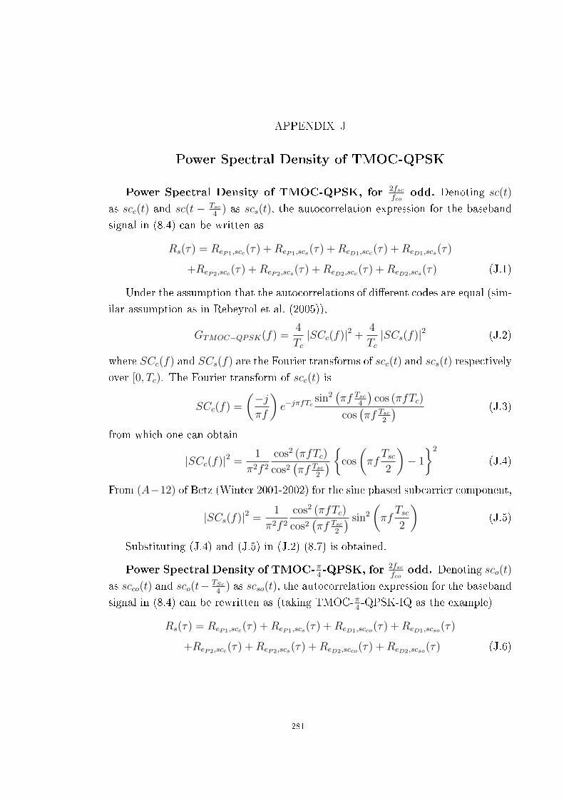
APPENDIX J
Power Spectral Density of TMOC-QPSK
Power Spectral Density of TMOC-QPSK, for 2fscfco
odd. Denoting sc(t)
as scc(t) and sc(t − Tsc4
) as scs(t), the autocorrelation expression for the baseband
signal in (8.4) can be written as
Rs(τ) = ReP1,scc(τ) +ReP1,scs(τ) +ReD1,scc(τ) +ReD1,scs(τ)
+ReP2,scc(τ) +ReP2,scs(τ) +ReD2,scc(τ) +ReD2,scs(τ) (J.1)
Under the assumption that the autocorrelations of di�erent codes are equal (sim-
ilar assumption as in Rebeyrol et al. (2005)),
GTMOC−QPSK(f) =4
Tc|SCc(f)|2 +
4
Tc|SCs(f)|2 (J.2)
where SCc(f) and SCs(f) are the Fourier transforms of scc(t) and scs(t) respectively
over [0, Tc). The Fourier transform of scc(t) is
SCc(f) =
(−jπf
)e−jπfTc
sin2(πf Tsc
4
)cos (πfTc)
cos(πf Tsc
2
) (J.3)
from which one can obtain
|SCc(f)|2 =1
π2f 2
cos2 (πfTc)
cos2(πf Tsc
2
) {cos
(πf
Tsc2
)− 1
}2
(J.4)
From (A−12) of Betz (Winter 2001-2002) for the sine phased subcarrier component,
|SCs(f)|2 =1
π2f 2
cos2 (πfTc)
cos2(πf Tsc
2
) sin2
(πf
Tsc2
)(J.5)
Substituting (J.4) and (J.5) in (J.2) (8.7) is obtained.
Power Spectral Density of TMOC-π4-QPSK, for 2fsc
fcoodd. Denoting sco(t)
as scco(t) and sco(t− TSc4
) as scso(t), the autocorrelation expression for the baseband
signal in (8.4) can be rewritten as (taking TMOC-π4-QPSK-IQ as the example)
Rs(τ) = ReP1,scc(τ) +ReP1,scs(τ) +ReD1,scco(τ) +ReD1,scso(τ)
+ReP2,scc(τ) +ReP2,scs(τ) +ReD2,scco(τ) +ReD2,scso(τ) (J.6)
281

282 J. POWER SPECTRAL DENSITY OF TMOC-QPSK
Hence, the power spectral density can be expressed as
GTMOC−π4−QPSK(f) =
2
TC|SCc(f)|2 +
2
TC|SCs(f)|2 +
2
TC|SCco(f)|2 +
2
TC|SCso(f)|2
(J.7)
Now with 2p = 2fscfco
,
sc(t) =
2p−1∑k=0
(−1)k µTsc2
(t− kTsc
2
)(J.8)
where, for the cosine phased π4phase-shifted subcarrier scco(t),
µTsc2
(t) =
1[0, Tsc
8
)−1
[Tsc8, Tsc
2
) (J.9)
The Fourier transform SCco(f) can be derived as
SCco(f) =
(1
πf
)e−jπf
Tsc8 e−j(
2TcTsc−1)πf Tsc
2cos (πfTc)
cos(πf Tsc
2
) ·[sin
(πf
Tsc8
)− e−jπf Tsc2 sin
(3πf
Tsc8
)](J.10)
For the sine phased π4phase-shifted subcarrier scs(t),
µTsc2
(t) =
1[0, 3Tsc
8
)−1
[3Tsc
8, Tsc
2
) (J.11)
and it can be shown that SCso(f) evaluates to the same expression as (J.10). Hence
|SCco(f)|2 = |SCso(f)|2 =1
π2f 2
cos2 (πfTc)
cos2(πf Tsc
2
) ·[cos2
(πf
Tsc2
)− 2 cos
(πf
Tsc2
)cos
(πf
Tsc4
)+ 1
](J.12)
Substituting (J.12), (J.4) and (J.5) in (J.7) (8.8) is obtained.

APPENDIX K
Output of the Correlator and Reference Signal Correlations
With (8.10) as one input and s(t− τ) = sI(t− τ)− jsQ(t− τ) as the other input,
the output of the reference signal mixer can be written as
y(t) =A√2{[sI(t− τ)sI(t− τ) cos (∆ωdt+ ∆θ) + sQ(t− τ)sQ(t− τ) cos (∆ωdt+ ∆θ)]
+j [sQ(t− τ)sQ(t− τ) sin (∆ωdt+ ∆θ) + sI(t− τ)sI(t− τ) sin (∆ωdt+ ∆θ)]
+ [sI(t− τ)sQ(t− τ) sin (∆ωdt+ ∆θ)− sQ(t− τ)sI(t− τ) sin (∆ωdt+ ∆θ)]
− j [sI(t− τ)sQ(t− τ) cos (∆ωdt+ ∆θ)− sQ(t− τ)sI(t− τ) cos (∆ωdt+ ∆θ)]}+ny(t) (K.1)
The output of the accumulator is
zk =
kTcoh∫(k−1)Tcoh
y(t)dt (K.2)
The individual correlations between the baseband component of the input signal
and the corresponding component of the reference signal have to be evaluated. Since
the baseband component and the reference signal component depend on the type of
modulation, one needs to evaluate all the four correlations present in (K.1) for the
three types of modulations viz. AltBOC, TMOC-QPSK and TMOC-π4-QPSK. One
example is shown here in detail and the results are provided for others. Consider the
�rst of the eight terms of (K.1) populated in (K.2). For AltBOC, with the subcarrier
signal representing the corresponding waveform (and neglecting the inter-modulation
product terms for simplicity), the baseband component of the input signal (real part
here) is
sI,AltBOC(t− τ) = eaI(t− τ)scI(t− τ) + eaQ(t− τ)scQ(t− τ)
+ebI(t− τ)scI(t− τ)− ebQ(t− τ)scQ(t− τ)
and the reference signal (real part) is
sI,AltBOC(t− τ) = eaI(t− τ)scI(t− τ) + eaQ(t− τ)scQ(t− τ)
−ebI(t− τ)scI(t− τ) + ebQ(t− τ)scQ(t− τ)
283

284K. OUTPUT OF THE CORRELATOR AND REFERENCE SIGNAL CORRELATIONS
Hence the �rst term of zk can be evaluated as
kTcoh∫(k−1)Tcoh
sI,AltBOC(t− τ)sI,AltBOC(t− τ) cos (∆ωdt+ ∆θ) dt =
Tcoh2
[RaI,aI (∆τ)RscI ,scI (∆τ) + 3Rc +RaQ,aQ (∆τ)RscQ,scQ (∆τ) + 3Rc
RbI,bI (∆τ)RscI ,scI (∆τ) + 3Rc +RbQ,bQ (∆τ)RscQ,scQ (∆τ) + 3Rc]·
sinc
(∆ωd
Tcoh2
)cos (∆θ)
=Tcoh
24R (∆τ)Rsc,AltBOC (∆τ) sinc
(∆ωd
Tcoh2
)cos (∆θ) + 12Rc (∆τ) (K.3)
where Rsc,AltBOC (∆τ) represents the combined correlations of all the subcarrier
pairs and Rc (∆τ) represents the cross correlation value of a single primary code
pair. It can be shown that the correlation between the subcarrier pairs are equal
i.e. RscI ,scI (∆τ) = RscQ,scQ (∆τ).
Similarly, the correlation due to sQ,AltBOC(t − τ)sQ,AltBOC(t − τ) can be shown
to be equivalent to (K.3). The correlation due to sI,AltBOC(t − τ)sQ,AltBOC(t − τ)
and sQ,AltBOC(t− τ)sI,AltBOC(t− τ) result in only cross correlation noise 12Rc. The
correlation between noise and the reference signal can be grouped together as n′(t) =∫ kTcoh(k−1)Tcoh
ny(t)s(t− τ)dt . Finally the output of the correlation can be written as
zk =√
2ATcohR (∆τ)Rsc,AltBOC (∆τ) sinc
(∆ωd
Tcoh2
)ej∆θ +R′ + n′ (t) (K.4)
where
Rsc,AltBOC (∆τ) = 8RscI ,scI (∆τ) (K.5)
and
R′ =A√2
24Rc (∆τ) sinc
(∆ωd
Tcoh2
)ej∆θ (K.6)
is the combined contribution due to the cross correlation terms.

APPENDIX L
Approximation Tables
The criteria for the best possible representation are (a) the error for all possible
representations for a given bit-width should be small and (b) the representation
values themselves should be small. Moreover if the errors in any two possible repre-
sentations are small and comparable to each other, then criterion (b) is given higher
priority. This is because, it is better to use the smaller values so that the growth
of the �nal correlation value after code mixing is kept to a minimum. For example
given 4 bits, {±1.2071,±0.5} can be represented either as {±5,±2} which results
in an error of 3.55% or as {±7,±3} which results in an error of 3.35%. Since the
di�erence between both the errors are negligible, {±5,±2} is selected according to
criterion (b). In the last column, the percentage error is calculated as (actual ratio -
integer representation ratio)/actual ratio.
Table L.1. Scaled integer approximations for {±1.2071,±0.5}
Bit-width Best possible representation % Error
(2's complement) ±1.2071 ±0.52 ±1 ±1 58.58
3 ±2 ±1 17.16
4 ±5 ±2 3.55
5 ±12 ±5 0.59
6 ±29 ±12 0.10
7 ±41 ±17 0.10
Table L.2. Scaled integer approximations for {±1,±0.7071}
Bit-width Best possible representation % Error
(2's complement) ±1 ±0.70712 ±1 ±1 29.29
3 ±3 ±2 6.07
4 ±7 ±5 1.00
5 ±14 ±10 1.00
6 ±17 ±12 0.17
7 ±58 ±41 0.03
285