A radio wave scattering algorithm and irregularity model for scintillation predictions

A radio wave scattering algorithm and irregularity model

for scintillation predictions

Emanoel Costa

Centro de Estudos em Telecomunicaco00es, Pontifıcia Universidade Catolica do Rio de Janeiro, Rio de Janeiro, Brazil

Santimay Basu

Space Vehicles Directorate, Air Force Research Laboratory, Hanscom Air Force Base, Massachusetts, USA

Received 23 May 2001; revised 3 October 2001; accepted 10 October 2001; published 27 June 2002.

[1] An algorithm for calculations of phase and amplitude scintillation of satellite signalsin the equatorial region will be described in detail. The algorithm will be developed byinitially transforming the discrete version of the Huygens-Fresnel integral into aconvolution involving a series of coefficients with decreasing amplitudes. Next, theFourier transform of the corresponding series of coefficients is stored for all thefrequencies of interest, and the fast Fourier transform algorithm is used to evaluate discreteconvolutions. Two phase screen models will be described. The first assumes that the phasefluctuations of the wave front emerging from the bottom of the irregularity layer areproportional to electron density fluctuations directly obtained from satellite in situmeasurements. The second assumes that the same phase fluctuations can be obtained fromtheir power spectral densities and phase spectra, represented by analytical functions withparameters provided by physics-based or morphological models of ionosphericirregularities. The propagation algorithm will be applied to both phase screen models,assuming five frequencies in the high-VHF to low-SHF band (suffering strong to weakscattering), to display its potential in the prediction of phase and amplitude scintillation ofsatellite signals. INDEX TERMS: 2439 Ionosphere: Ionospheric irregularities; 2447 Ionosphere:

Modeling and forecasting; 2487 Ionosphere: Wave propagation (6934); KEYWORDS: ionospheric irregularity,

radio wave scattering, phase screen, amplitude scintillation, phase scintillation

1. Introduction

[2] The phase-screen theory has been frequently usedto study the fluctuations of a radio signal due to itspropagation through an irregularity layer in the iono-sphere. This theory assumes that the medium is equiv-alent to a diffracting screen with random phasefluctuations that are proportional to the irregularities inthe total electron content. The theory further assumesthat the phase fluctuations are frozen in the uniformbackground and move with a fixed velocity. As the wavepropagates in free space beyond the screen, fluctuationsin amplitude begin to develop. This approach was usedby many authors to derive different moments of theamplitude and the phase of the received signal [Bowhill,1961; Mercier, 1962; Briggs and Parkin, 1963; Budden,1965; Salpeter, 1967; Tatarskii, 1971; Yeh and Liu,

1982]. These analytical studies were performed both inthe thin-screen (small RMS phase fluctuation) and in thethick-screen (large RMS phase fluctuation) regimes,assuming appropriate statistics for the phase fluctuationsof the emerging wave front.[3] An alternative to the above analytical studies is the

application of the Huygens-Fresnel diffraction theory[Goodman, 1968] to an irregular ionosphere representedby single or multiple phase screens to numerically char-acterize the signals received on the ground. This approachrepeatedly applies the known field at a certain screen intoa convolution integral to determine the field at the nextscreen. It can be used when scattering is relatively strongand can also be applied to a diffracting screen with phasefluctuations characterized from in situ measurements orby models assuming arbitrary shapes for their powerspectral densities [Knepp, 1983; Rino and Owen, 1984].The most general version of this approach is equivalent tothe numerical solution of the parabolic equation thatdescribes wave propagation when partial reflection can

RADIO SCIENCE, VOL. 37, NO. 3, 1046, 10.1029/2001RS002498, 2002

Copyright 2002 by the American Geophysical Union.

0048-6604/02/2001RS002498

18 - 1

be neglected [Wagen and Yeh, 1989; Martin, 1993]. Thisequation has been solved directly, using classical techni-ques such as the Crank-Nicholson algorithm [Wernik etal., 1980]. It can also be solved by the Fourier split-stepalgorithm [Kuttler and Dockery, 1991].[4] In addition to the known field the Huygens-Fresnel

convolution integral involves a unit-amplitude term thatoscillates increasingly faster. Therefore a threshold willbe eventually reached beyond which the field can beconsidered as a constant within each cycle of the secondterm. The numerical evaluation of the integral shouldonly be performed up to this threshold. Otherwise, thefast oscillations in the second term will not be adequatelysampled, and errors will rapidly accumulate. However,since the second term of the convolution integral has unitamplitude, it is not so easy to determine this threshold.One of the main objectives of this paper is to show thatthe discrete version of the Huygens-Fresnel integral canbe written as the convolution between a series ofsampled values of the field and a series of coefficientswith decreasing amplitudes. The use of these coefficientsprovides an alternative approach that is capable ofcircumventing the described difficulty. Additionally, anefficient propagation algorithm can be designed by apriori calculating these coefficients and storing the Four-ier transform of the corresponding series for all thefrequencies of interest, combined with use of the fastFourier transform (FFT) algorithm to evaluate discreteconvolutions.[5] Sections 2–5 will also describe models for the

phase fluctuations in a diffracting screen and will applythe designed algorithm to the prediction of phase andamplitude scintillation of satellite signals in the equatorialionosphere. The phase screen models and the propagationalgorithm can be easily integrated with physics-based ormorphological models of ionospheric irregularities toforecast equatorial scintillation.

2. Slant Propagation Through an

Irregularity Layer

[6] The slant propagation of a plane wave through abidimensional irregularity layer of thickness L and bot-tom height h can be represented by the wave equation

@2U

@ x2þ @2U

@ z2þ k 2n2U ¼ 0: ð1Þ

In the above equation, k is the free space wave numberand n is the refractive index of the medium. The horizontalx axis is aligned with the bottom of the layer, and the z axispoints downward. Without any loss of generality the fieldU(x, z) can be represented by

U x; zð Þ ¼ u x; zð Þeik sin q xþcos q zð Þ; ð2Þ

where q is the zenith angle of the wave vector.Substituting the right-hand side of equation (2) for Uinto equation (1) and assuming that the scale size of thevertical fluctuations of the complex amplitude u is largein comparison with (2k cos q)�1, one gets

@2u

@ x2þ 2ik sin q

@ u

@ xþ cos q

@ u

@ z

� �þ k 2 n2 � 1

� �u ¼ 0: ð3Þ

Under the above approximation the second derivative ofu with respect to z becomes much smaller than the thirdterm in equation (3) and can be discarded. Thisapproximation is reasonable for sufficiently highfrequencies and small zenith angles. It is seen that theslant propagation of the plane wave is now representedby a parabolic equation, indicating that backscatteringhas been neglected.[7] The Fourier split-step algorithm [Kuttler and Dock-

ery, 1991] can be used to numerically solve equation (3).This algorithm assumes that u(x, �L) = 1, divides thelayer into thin horizontal slabs, and substitutes the Four-ier representation

u x; zð Þ ¼ 1

2p

Zþ1

�1

~u p; zð Þeipxdp ð4Þ

into equation (3) to obtain

@~u

@zþ k2 n2 � 1ð Þ � 2kp sin q� p2

2ik cos q~u ¼ 0: ð5Þ

Equation (5) yields

~u p; zþ dzð Þ ¼ ~u p; zð Þ exp ik n2 � 1ð Þ2cos q

dz� �

�exp �ip2 þ 2 kp sin q

2 k cos qdz

� �: ð6Þ

Calculating the inverse Fourier transform of the aboveequation, it follows that

u xþ tan q dz; zþ dz;ð Þ ¼ exp ik n2 � 1ð Þ2 cos q

dz� �

�ffiffiffiffiffiffiffiffiffiffiffiffiffik cos qi 2p dz

r( Zþ1

�1

u x0; zð Þexp ik cos q2dz

x� x0ð Þ2� �

dx0

)

¼ exp ik n2 � 1ð Þ2 cos q

dz� �

n x; zþ dzð Þ: ð7Þ

In the above equation, dz is the step size. Thisequation should be repeatedly applied to produce thefield from the top to the bottom of the layer. It shouldthen be applied once more with dz = h and n = 1 toproduce the field on the ground. It should be observed

18 - 2 COSTA AND BASU: RADIO WAVE SCATTERING ALGORITHM AND IRREGULARITY MODEL

that each step in the solution of the parabolic equationby the Fourier split-step algorithm begins with theapplication of the Huygens-Fresnel diffraction integralwithin curly brackets [Goodman, 1968] to the field atthe top of each slab. A phase shift and a displacementare then performed to produce the field at the bottomof the same slab. Note that phase shift and thedisplacement are not necessary when n = 1 and q = 0�,respectively.[8] Equation (7) is only an exact solution to the para-

bolic equation (3) when (n2 � 1) is constant. There areerrors associated with the above solution when therefractive index is position-dependent [Knepp, 1983],which is the case of interest. Adapting the derivationby Kuttler and Dockery [1991] to slant propagation ofplane waves through an irregularity layer in the iono-sphere, one obtains the following conditions for negli-gible errors in each step:

dz 2ffiffiffiffiffiffiffiffiffifficos q

p ffiffiffiffiffiffiffiffiffiffiffiffiffiffiffiffin2 � 1j j

p@ n2�1j j

@x

; 2k cos qn2 � 1 @ n2�1j j

@x

u@u@x

: ð8Þ

In their application of equation (7) to propagation in thetroposphere (with q = 0�) the first upper bound in theright-hand side of inequality (8) was equal to 20 km.Kuttler and Dockery claimed that their numericalexperiments using the Fourier split-step algorithmrevealed that the ratio within the absolute value barsin the second upper bound is greater than 1, except inthe vicinities of nulls in the field. Additionally, theyclaimed that the dimensions and the number of thesevicinities increase with the frequency. As a result, themaximum acceptable value for dz should decrease withthe frequency. Kuttler and Dockery [1991] thenreminded their readers that the total error in thecalculations depended on the accumulation of the errorsfrom each step. No analytical treatment of erroraccumulation is available. However, they observed thatstep sizes of several hundred wavelengths wereadequate for the convergence of the solution in theirapplication and presented an excellent agreementbetween corresponding results from the Fourier split-step algorithm and from a waveguide mode propagationmodel.[9] In the application of the Fourier split-step algo-

rithm to analyze the slant propagation of plane wavesthrough an irregularity layer in the ionosphere, the upperbounds in the right-hand side of inequality (8) can berewritten in the forms

dzkm223fMHz LNð Þmffiffiffiffiffiffiffiffiffifficos q

p ffiffiffiffiffiffiffiffiffiffiNm�3

p.;

0:0419 fMHz LNð Þmcos q u�

@u

@x

km

; ð9Þ

where N is the electron density and LN is its gradientscale size, if upper VHF or even higher frequenciesare assumed. The minimum value of LN has beenestimated, on the basis of a reconstruction of the high-resolution electron density in situ data displayed byMcClure et al. [1977], to be of the order of 200 m.Therefore the first upper bound for the step size in thepresent application is consistent with the valueobtained by Kuttler and Dockery [1991]. Consideringthe arguments presented in the previous paragraph inrelation to the second bound, one could expect thatstep sizes of several hundred wavelengths would alsobe adequate for the convergence of the solution in thepresent application. However, it is important toobserve the convergence of the solution as the stepsize is reduced to determine a value of dz that isadequate to the present application.[10] It has already been mentioned that the maximum

acceptable value for dz should decrease with the fre-quency. This will increase the processing time necessaryto perform the calculations. Additionally, the secondterm in the convolution integral within curly bracketsin equation (7) oscillates increasingly faster with |x � x0|,and this behavior is intensified as the frequency of theplane wave also increases. Therefore, in the evaluation ofthe convolution integral, a threshold in |x � x0| will bereached beyond which these oscillations become so fastthat u(x0, z) can be considered a constant within eachcycle of the second term. Beyond this threshold, whichcharacterizes an effective integrating interval, the con-tribution of the integrand becomes negligible and can bediscarded. Note that the length of the effective integrat-ing interval decreases (indicating that propagationbecomes increasingly localized) as the frequencyincreases, approaching the optical regime.[11] The straightforward numerical evaluation of the

convolution integral should only be performed over theeffective integrating interval; that is, it should be asso-ciated with truncation. Otherwise, the fast oscillations inthe second term of the convolution integral will not beadequately sampled (assuming a uniform sampling), anderrors will rapidly accumulate. Simply decreasing thesampling interval will only delay the beginning of theerror accumulation process, in addition to unnecessarilyincreasing the processing time spent in the calculations.However, note that all the sampled elements of thesecond term of the convolution integral in equation (7)have unit amplitudes. Therefore it is not easy to deter-mine the length of the effective integrating interval in thex domain.[12] In section 3 the discrete version of the integral will

be written as the convolution between a series ofsampled values of the plane wave at a fixed height anda series of coefficients with decreasing amplitudes. Theuse of these coefficients provides an alternative approach

COSTA AND BASU: RADIO WAVE SCATTERING ALGORITHM AND IRREGULARITY MODEL 18 - 3

that is capable of circumventing the difficulty describedin the previous paragraph.

3. Description of the Scattering Algorithm

[13] As mentioned in section 2, the term within curlybrackets in equation (7), denoted v(x, z + dz), results fromthe convolution of two functions. Therefore it has adiscrete representation that can be written in the form

vm zþ dzð Þ ¼XQq¼�Q

Cqum�q: ð10Þ

In the above equation, m and q play roles analogous tothose of x and x0 in equation (7), respectively. Equation(10) allows an efficient calculation of the signal vm(z +dz) through an ‘‘a priori’’ calculation of the coefficientsCq and the storage of the Fourier transform of thecorresponding series for each frequency of interest,combined with use of the FFT algorithm to evaluatediscrete convolutions.[14] To derive an expression for the coefficients Cq

displaying decreasing absolute values with the index q,the horizontal variables x and x0 will be initially normal-ized by the horizontal sampling interval dx. That is, thechanges of variables x = mdx and x0 = s dx will beintroduced into equation (7), and the result will bewritten as a summation of integrals over unit s-intervalsas follows:

vm zþ dzð Þ ¼ffiffiffiffiffig

ip

r Xþ1

n¼�1

Znþ1

n

u s; zð Þeig m�sð Þ2ds

g ¼ 2pcos q dx�zf

� �2;

ð11Þ

where zf = (2l dz)1/2 is the Fresnel scale size and l is thewavelength of the transmitted signal.[15] It will then be assumed that u(s, z) is a piecewise

linear function of the first variable, with breakpoints at itsinteger values. That is,

u s; zð Þ¼ nþ1ð Þun�n unþ1þ unþ1�unð Þs n� s � nþ1:

ð12Þ

Note that the samples un and un+1 are obtained at thealtitude z. To simplify notation, this dependence has beenomitted in expression (12). Substituting its right-handside for u(s, z) in equation (11), it follows that

vm zþ dzð Þ ¼ 1ffiffiffiffi2i

pXþ1

n¼�1nþ 1ð ÞI1m�n � I2m�n

� �un

(

�Xþ1

n¼�1n I1m�n � I2m�n

� �unþ1

); ð13Þ

where

I1m�n ¼ffiffiffiffiffiffi2g

p

r Znþ1

n

eig m�sð Þ2ds ¼Zb m�nð Þ

b m�n�1ð Þ

ei p=2ð ÞV2dV;

ð14Þ

I2m�n ¼ffiffiffiffiffiffi2g

p

r Znþ1

n

s eig m�sð Þ2ds ¼ m I1m�n

þffiffiffiffiffiffi2g

p

r Znþ1

n

m� sð Þ eig m�sð Þ2d m� sð Þ

¼ mI1m�n �1

b

Zb m�nð Þ

b m�n�1ð Þ

V ei p=2ð ÞV2dV ¼ mI1m�n � J 2m�n;

ð15Þ

b ¼ffiffiffiffiffiffiffiffiffiffiffi2g=p

p¼ 2

ffiffiffiffiffiffiffiffiffifficos q

pdx�zf : ð16Þ

[16] Substituting the right-hand side of equation (15)for I2m � n in equation (13), collecting terms that multiplythe same sample un in this equation (or, equivalently,changing indices n +1! n in the second summation), onegets

vm zþ dzð Þ ¼ 1ffiffiffiffi2i

pXþ1

n¼�1n� mþ 1ð ÞI1m�n

�� m� nþ 1ð ÞI1m�nþ1 þ J 2m�n � J 2m�nþ1�un:

ð17Þ

A final change of indices n = m � q yields

vm zþ dzð Þ ¼Xþ1

q¼�1

1ffiffiffiffi2i

p �qþ 1ð ÞI1q � qþ 1ð Þh�

I1qþ1

þJ 2q �J 2qþ1

i�um�q: ð18Þ

It should be observed that the above equation has exactlythe same format as equation (10) and that its term withincurly brackets should be identified with the coefficientCq.[17] The right-hand side of equation (14) can be

written in terms of Fresnel integrals [Abramowitz andStegun, 1972]

I1q ¼Zbq

b q�1ð Þ

ei p=2ð ÞV2dV ¼ C bqð Þ � C b q� 1ð Þ½ � þ iS bqð Þ

�iS b q� 1ð Þ½ �: ð19Þ


On the other hand, a straightforward integration yields

J 2q ¼ 1

b

Zbqb q�1ð Þ

V ei p=2ð ÞV2dV ¼ �iei p=2ð Þ bqð Þ2 � ei p=2ð Þ b q�1ð Þ½ �2

pb:

ð20Þ

Substituting the right-hand sides of expressions (19) and(20) for Iq

1 and Jq2, respectively, into the term within

curly brackets in expression (18), with appropriateconsideration for their indices, one gets

Cq ¼ Cqþ1 bð Þ þ Cq�1 bð Þ � 2Cq bð Þ; ð21Þ

where

Cq bð Þ ¼ 1ffiffiffiffi2i

pp b

p bqð Þ C bqð Þ þ iS bqð Þ½ � þ iei p=2ð Þ bqð Þ2n o

:

ð22Þ

Computationally, it is convenient to express the Fresnelintegrals in expression (22) in terms of the auxiliaryfunctions f (bq) and g(bq) [Abramowitz and Stegun,1972]. Therefore

C0 ¼ 1þ 2 c1 bð Þ � c0 bð Þright�;½ ð23Þ

Cq ¼ cqþ1 bð Þ þ cq�1 bð Þ � 2cq bð Þ; ð24Þwhere

cq bð Þ ¼ 1ffiffiffiffi2i

pp b

p bqð Þf bqð Þ � 1½ �sin p2

bqð Þ2h in

� p bqð Þg bqð Þ½ �cos p2

bqð Þ2h io

� i1ffiffiffiffi2i

pp b

p bqð Þf bqð Þ � 1½ �cos p2

bqð Þ2h in

þ p bqð Þg bqð Þ½ �sin p2

bqð Þ2h io

: ð25Þ

The coefficients cq(b) can be calculated using both thesmall-argument and asymptotic expansions for f (x) andg(x) provided by Abramowitz and Stegun [1972].Expression (24) indicates that the coefficients Cq canbe obtained iteratively. More specifically, since thevalues cq�1(b) and cq(b) are available from previousiterations, only the value of cq+1(b), calculated usingexpression (25), is necessary to obtain Cq. Note that inaddition to this prescription (that is, in addition to c1(b)),c0(b) should also be calculated to produce C0 at the firstiteration.[18] From expressions (21) and (22), as well as from

the properties of the Fresnel integrals (both are oddfunctions of their arguments), it can be shown that Cq

= C�q. Furthermore, the dominant terms in the asymp-

totic expansions of the auxiliary functions f (bq) andg(bq) are such that [Abramowitz and Stegun, 1972]

p bqð Þf bqð Þ � 1 e �3

p bqð Þ2h i2 ; ð26Þ

and

p bqð Þg bqð Þ e 1

p bqð Þ2: ð27Þ

Therefore the dominant term in the asymptotic expansionof the coefficient cq(b) is

cq bð Þ e � 1ffiffiffiffi2i

ppb

ei p=2ð Þ bqð Þ2

p bqð Þ2: ð28Þ

It is seen that the absolute value of cq(b) decreasesasymptotically with the second power of the index q andthe third power of the parameter b. Expression (24)shows that Cq is the second central difference of cq(b).Therefore it should decrease asymptotically at least asfast as the right-hand side of expression (28), as desired.

4. Phase Screen Models

[19] The scattering algorithm will be applied todescribe the slant propagation through an irregularitylayer, represented by two different phase screen models.These phase screen models characterize an irregularitylayer by its bottom height h (also the height of phasescreen), the thickness L and the average electron densityNo and neglect amplitude fluctuations in the wave frontemerging from the bottom of the irregularity layer.[20] The first phase screen model assumes that the

phase fluctuations j(x) of the wave front emerging fromthe bottom of the irregularity layer are proportional toelectron density fluctuations dN(x) resulting from satel-lite in situ measurements such as those reported in theliterature [McClure et al., 1977; Basu et al., 1983]. As anexample of the first model, Figure 7 of McClure et al.[1977], displaying electron density fluctuations detectedby the AE-C satellite was enlarged and digitized. Next, itwas sampled at a constant interval to simulate a samplingdistance of in situ measurements equal to 40 m. Finally,it was low-pass filtered to remove digitization-inducednoise.[21] The thick solid curve in the upper panel of Figure 1

shows the normalized (zero-mean, unit standard devia-tion) phase fluctuation function j(x) resulting from thismodel. The middle panel of Figure 1 shows the corre-sponding maximum-entropy method (MEM) powerspectrum (thick solid curve). This curve displays anouter scale size Lo � 25.0 km and a power law spectralindex p = 1.86 for spatial frequencies between fo = 1/Lo


� 0.04 km�1 and a breakpoint located at the spatialfrequency fb = 1/Lb � 2.50 km�1. For spatial frequencieshigher than fb a power law spectral index q = 3.00 isobserved. These parameters are consistent with the onesobtained by Basu et al. [1983], except for the spatialfrequency fb, which surpasses their highest value. On the

other hand, rocket in situ electron density data [Hysellet al., 1994; Hysell, 2000] from altitudes above 280 kmhave shown double-slope spectra with spectral indicesbetween 1.7 and 2.5 for large-scale sizes and between 4.5and 5.0 for small-scale sizes. The scale size of thespectral breakpoint has been found in the vicinity of

Figure 1. (top) Normalized phase fluctuations j(x) resulting from the first model (thick curve,in situ data reproduced from McClure et al. [1977]) and the second model (thin curve), assumingfo = 0.04 km�1, fb = 2.50 km�1, p = 1.86, and q = 3.00). (middle) Corresponding MEM powerspectral densities (same curve code). (bottom) Corresponding phases of the FFT components afterthe original ±p discontinuities have been eliminated, and the resulting curve has been artificiallybroken into sections, to allow the phase curve to be displayed within the selected vertical scale(same curve code).


100 m (spatial frequency fb = 10 km�1). These resultsseem to indicate that spread F irregularities sampled inthe east-west direction by satellites display power spectrawith larger breakpoint scale sizes and smaller slopes inthe small-scale size regime than those obtained fromsampling the same irregularities in the vertical directionby rockets.[22] The lower panel of Figure 1 shows the phase y( fx)

of the FFT components of j(x) as a function of the spatialfrequency fx (thick curve). Initially, the original ±p dis-continuities have been eliminated to produce a continuouscurve that fits (in the least squares sense) the function

y fxð Þ ¼ p� 66:166 fx þ 1:434 f 2x ð29Þ

with RMS error equal to 7.80 rad. Next, the resultingcurve has been artificially broken into sections, to allowall the phase curve to be displayed within the selectedvertical scale.[23] The second phase screen model assumes that the

power spectral density function Sj( fx) of the phasefluctuations j(x) is represented by

Sj fxð Þ ¼ 1 fx � fo; ð30aÞ

Sj fxð Þ ¼ fx=foð Þ�pfo < fx � fb; ð30bÞ

Sj fxð Þ ¼ fb=foð Þ�pfx=fbð Þ�q

fb < fx: ð30cÞ

The second phase screen model initially generates F( fx),a realization of the desired phase fluctuation j(x) in theFourier transform domain, using

F fxð Þ ¼ Sj fxð Þ� �1=2

eiy fxð Þ: ð31Þ

That is, the square root of the right-hand side of expression(30)–(30c) is sampled at equally spaced spatial frequen-cies, and each sample is multiplied by a phase factorcharacterized by a prescribed random variable y( fx)[Franke and Liu, 1983]. The inverse Fourier transform ofexpression (31) then provides a realization of the randomphase fluctuations j(x) at the bottom of the irregularitylayer. Fougere [1985] used a more involved approach forthe generation of j(x).[24] The example using the second model assumes that

Lo = 1/fo = 25.0 km, Lb = 1/fb = 0.40 km, p = 1.86, andq = 3.00, which are the parameters of the first model. Italso assumes that the samples of y( fx) are mutuallyindependent random variables uniformly distributedbetween 0 and 2p. Additionally, attempts have beenmade to use the second model to produce realizationsof j(x) that display phase distributions of their FFTcomponents closely matching that of the first model.The thin solid curves in the three panels of Figure 1display the corresponding results.[25] It should be observed that the normalized phase

screen curve created from the in situ data is character-

istically different from the results provided by the secondmodel. The thick curve in the upper panel of Figure 1displays, particularly in the first 15 km of data, asym-metric structures with steep edges. Many rocket [Kelleyet al., 1976; Morse et al., 1977; Hysell et al., 1994] andsatellite data [Dyson et al., 1974; Basu et al., 1983] alsoshow similar features. These were accepted as an indi-cation that steep edges resulting from the nonlinearsteepening of individual waves by plasma instabilityprocesses could dominate the power spectrum of theelectron density fluctuations and produce the observedspectral shape [Costa and Kelley, 1978; Wernik et al.,1980]. This process would exhibit some degree of self-similar scale invariance and of coherence in the phasedistribution of the Fourier components of the electrondensity fluctuations [Costa and Kelley, 1978; Hysellet al., 1994]. On the other hand, the asymmetric struc-tures with steep edges are not present in the thin curve ofthe upper panel, which is more representative of aturbulence-like process, also resulting in essentially thesame power spectrum for the wave amplitudes, but withuniformly distributed random phase.[26] The realizations provided by the models should

then be adjusted for the proper average fluctuationamplitude. They are normalized to create a zero-mean,unit standard deviation series of values, which are thenmultiplied by [Costa and Kelley, 1977; Rino, 1979]

C ¼ G relð ÞffiffiffiffiffiffiffiffiffiffiffiffiffiffiffiffiffiLoL sec q

pNo

dN2� �N 2o

� �1=2: ð32Þ

In the above expression, re = 2.8179 � 10�15 m is theclassical electron radius, l is the wavelength, and q is thezenith angle of the incident rays. Further, Lo, L, and No

have been previously defined, and hdN2i is the varianceof the (zero-mean) electron density fluctuations. That is,the last term in expression (32) is the fractional RMSelectron density fluctuation. Naturally, the parametersassociated with the first model are defined by the data setin this case and, to make the overall model self-consistent, should be used in expression (32). Finally,the geometric factor G combines the effects of theanisotropy in the three-dimensional power spectraldensity of the electron density fluctuations with theorientation of the propagation direction with respect tothe geomagnetic field [Rino, 1979].

5. Amplitude and Phase Scintillation of the

Signal Received on the Ground

[27] Figure 2 displays the variations with the index qand the frequency of the absolute values of the coef-ficients Cq (decibels) defined in equations (10) and (23)to (25), assuming h = 400 km, dx = 40 m, q = 30�, andf = 136 MHz, 360 MHz, 800 MHz, 1500 MHz, 4000


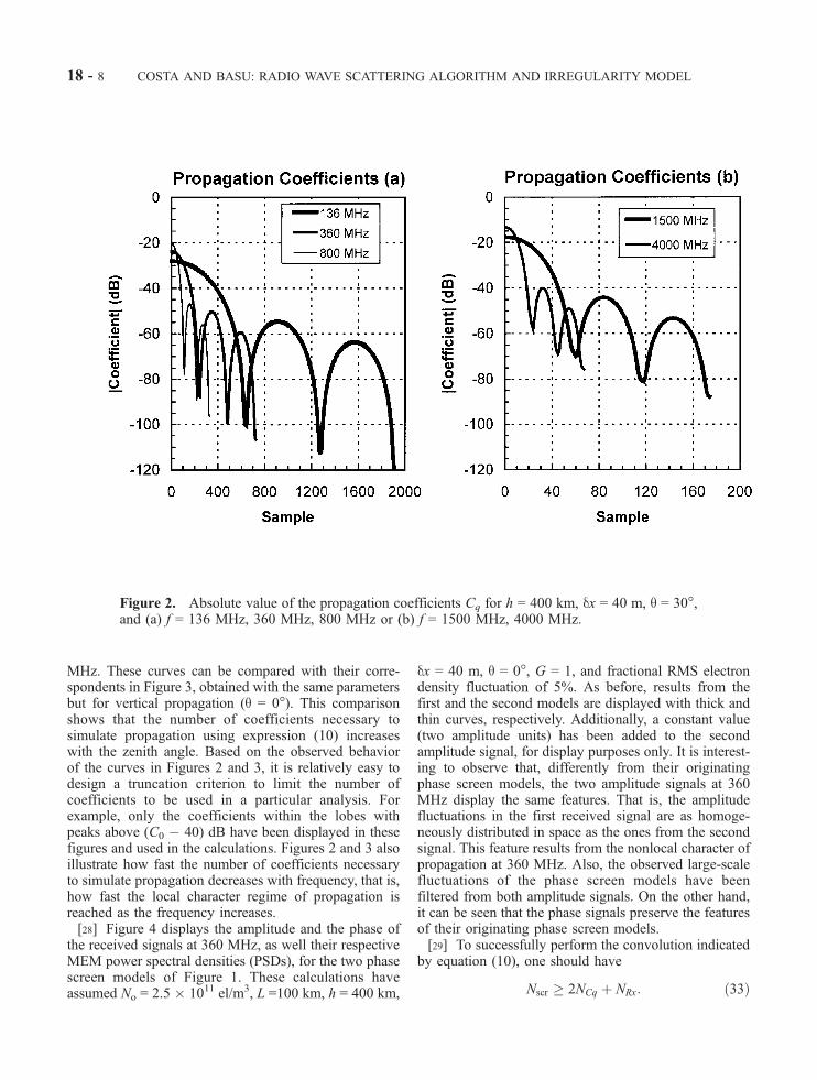
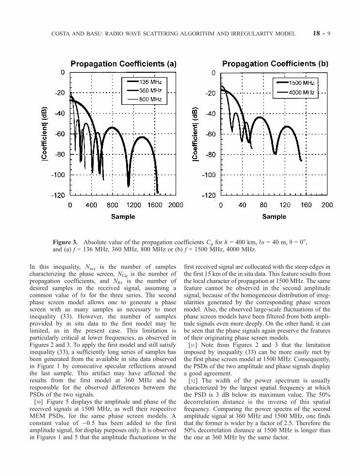
MHz. These curves can be compared with their corre-spondents in Figure 3, obtained with the same parametersbut for vertical propagation (q = 0�). This comparisonshows that the number of coefficients necessary tosimulate propagation using expression (10) increaseswith the zenith angle. Based on the observed behaviorof the curves in Figures 2 and 3, it is relatively easy todesign a truncation criterion to limit the number ofcoefficients to be used in a particular analysis. Forexample, only the coefficients within the lobes withpeaks above (C0 � 40) dB have been displayed in thesefigures and used in the calculations. Figures 2 and 3 alsoillustrate how fast the number of coefficients necessaryto simulate propagation decreases with frequency, that is,how fast the local character regime of propagation isreached as the frequency increases.[28] Figure 4 displays the amplitude and the phase of

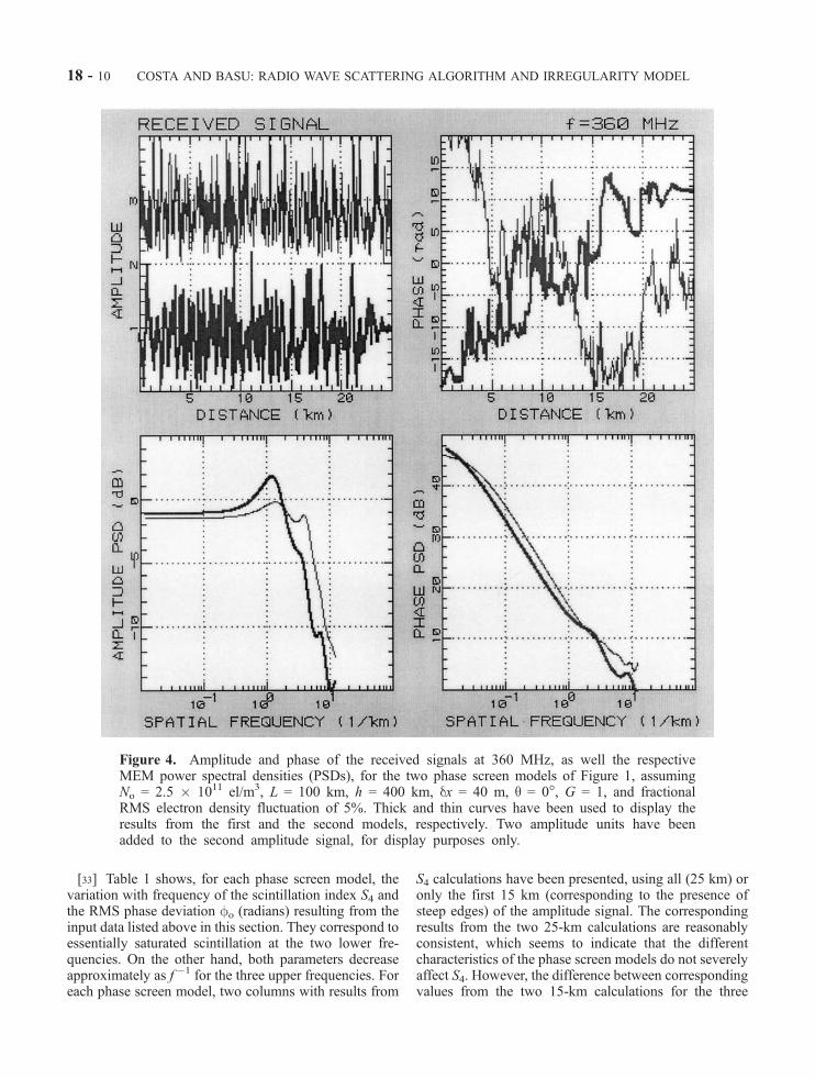
the received signals at 360 MHz, as well their respectiveMEM power spectral densities (PSDs), for the two phasescreen models of Figure 1. These calculations haveassumed No = 2.5 � 1011 el/m3, L =100 km, h = 400 km,

dx = 40 m, q = 0�, G = 1, and fractional RMS electrondensity fluctuation of 5%. As before, results from thefirst and the second models are displayed with thick andthin curves, respectively. Additionally, a constant value(two amplitude units) has been added to the secondamplitude signal, for display purposes only. It is interest-ing to observe that, differently from their originatingphase screen models, the two amplitude signals at 360MHz display the same features. That is, the amplitudefluctuations in the first received signal are as homoge-neously distributed in space as the ones from the secondsignal. This feature results from the nonlocal character ofpropagation at 360 MHz. Also, the observed large-scalefluctuations of the phase screen models have beenfiltered from both amplitude signals. On the other hand,it can be seen that the phase signals preserve the featuresof their originating phase screen models.[29] To successfully perform the convolution indicated

by equation (10), one should have

Nscr � 2NCq þ NRx: ð33Þ

Figure 2. Absolute value of the propagation coefficients Cq for h = 400 km, dx = 40 m, q = 30�,and (a) f = 136 MHz, 360 MHz, 800 MHz or (b) f = 1500 MHz, 4000 MHz.


In this inequality, Nscr is the number of samplescharacterizing the phase screen, NCq is the number ofpropagation coefficients, and NRx is the number ofdesired samples in the received signal, assuming acommon value of dx for the three series. The secondphase screen model allows one to generate a phasescreen with as many samples as necessary to meetinequality (33). However, the number of samplesprovided by in situ data to the first model may belimited, as in the present case. This limitation isparticularly critical at lower frequencies, as observed inFigures 2 and 3. To apply the first model and still satisfyinequality (33), a sufficiently long series of samples hasbeen generated from the available in situ data observedin Figure 1 by consecutive specular reflections aroundthe last sample. This artifact may have affected theresults from the first model at 360 MHz and beresponsible for the observed differences between thePSDs of the two signals.[30] Figure 5 displays the amplitude and phase of the

received signals at 1500 MHz, as well their respectiveMEM PSDs, for the same phase screen models. Aconstant value of �0.5 has been added to the firstamplitude signal, for display purposes only. It is observedin Figures 1 and 5 that the amplitude fluctuations in the

first received signal are collocated with the steep edges inthe first 15 km of the in situ data. This feature results fromthe local character of propagation at 1500MHz. The samefeature cannot be observed in the second amplitudesignal, because of the homogeneous distribution of irreg-ularities generated by the corresponding phase screenmodel. Also, the observed large-scale fluctuations of thephase screen models have been filtered from both ampli-tude signals even more deeply. On the other hand, it canbe seen that the phase signals again preserve the featuresof their originating phase screen models.[31] Note from Figures 2 and 3 that the limitation

imposed by inequality (33) can be more easily met bythe first phase screen model at 1500 MHz. Consequently,the PSDs of the two amplitude and phase signals displaya good agreement.[32] The width of the power spectrum is usually

characterized by the largest spatial frequency at whichthe PSD is 3 dB below its maximum value. The 50%decorrelation distance is the inverse of this spatialfrequency. Comparing the power spectra of the secondamplitude signal at 360 MHz and 1500 MHz, one findsthat the former is wider by a factor of 2.5. Therefore the50% decorrelation distance at 1500 MHz is longer thanthe one at 360 MHz by the same factor.

Figure 3. Absolute value of the propagation coefficients Cq for h = 400 km, dx = 40 m, q = 0�,and (a) f = 136 MHz, 360 MHz, 800 MHz or (b) f = 1500 MHz, 4000 MHz.


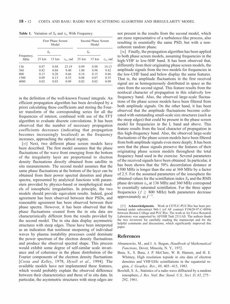
[33] Table 1 shows, for each phase screen model, thevariation with frequency of the scintillation index S4 andthe RMS phase deviation fo (radians) resulting from theinput data listed above in this section. They correspond toessentially saturated scintillation at the two lower fre-quencies. On the other hand, both parameters decreaseapproximately as f �1 for the three upper frequencies. Foreach phase screen model, two columns with results from

S4 calculations have been presented, using all (25 km) oronly the first 15 km (corresponding to the presence ofsteep edges) of the amplitude signal. The correspondingresults from the two 25-km calculations are reasonablyconsistent, which seems to indicate that the differentcharacteristics of the phase screen models do not severelyaffect S4. However, the difference between correspondingvalues from the two 15-km calculations for the three

Figure 4. Amplitude and phase of the received signals at 360 MHz, as well the respectiveMEM power spectral densities (PSDs), for the two phase screen models of Figure 1, assumingNo = 2.5 � 1011 el/m3, L = 100 km, h = 400 km, dx = 40 m, q = 0�, G = 1, and fractionalRMS electron density fluctuation of 5%. Thick and thin curves have been used to display theresults from the first and the second models, respectively. Two amplitude units have beenadded to the second amplitude signal, for display purposes only.


upper frequencies clearly shows the important effects ofsteep edges observed in the first phase screen model ongigahertz scintillation [Wernik et al., 1980].

6. Conclusion

[34] In this paper, the Huygens-Fresnel convolutionintegral has been explored to describe the slant prop-

agation of a plane wave through a bidimensional irreg-ularity layer. Instead of the straightforward application ofthe integral, one of the main contributions has been toshow that its discrete version can be transformed into aconvolution between a series of sampled values of thefield and a series of propagation coefficients withdecreasing amplitudes. These coefficients have beenexpressed in terms of the auxiliary functions involved

Figure 5. Amplitude and phase of the received signals at 1500 MHz, as well as the respectiveMEM power spectral densities (PSDs), for the two phase screen models of Figure 1, assumingNo = 2.5 � 1011 el/m3, L = 100 km, h = 400 km, dx = 40 m, q = 0�, G = 1, and fractionalRMS electron density fluctuation of 5%. Thick and thin curves have been used to display theresults from the first and the second models, respectively. A constant value (�0.5) has beenadded to the first amplitude signal, for display purposes only.


in the definition of the well-known Fresnel integrals. Anefficient propagation algorithm has been developed by apriori calculating these coefficients and storing the Four-ier transform of the corresponding series for all thefrequencies of interest, combined with use of the FFTalgorithm to evaluate discrete convolutions. It has beenobserved that the number of necessary propagationcoefficients decreases (indicating that propagationbecomes increasingly localized) as the frequencyincreases, approaching the optical regime.[35] Next, two different phase screen models have

been described. The first model assumes that the phasefluctuations of the wave front emerging from the bottomof the irregularity layer are proportional to electrondensity fluctuations directly obtained from satellite insitu measurements. The second model assumes that thesame phase fluctuations at the bottom of the layer can beobtained from their power spectral densities and phasespectra, represented by analytical functions with param-eters provided by physics-based or morphological mod-els of ionospheric irregularities. In principle, the twomodels should provide equivalent results. Indeed, goodagreement has been observed between their PSDs, andreasonable agreement has been observed between theirphase spectra. However, it has been observed that thephase fluctuations created from the in situ data arecharacteristically different from the results provided bythe second model. The in situ data display asymmetricstructures with steep edges. These have been interpretedas an indication that nonlinear steepening of individualwaves by plasma instability processes could dominatethe power spectrum of the electron density fluctuationsand produce the observed spectral shape. This processwould exhibit some degree of self-similar scale invari-ance and of coherence in the phase distribution of theFourier components of the electron density fluctuations[Costa and Kelley, 1978; Hysell et al., 1994]. Theavailable models have not implemented these features,which would probably explain the observed differencebetween their characteristics and those of in situ data. Inparticular, the asymmetric structures with steep edges are

not present in the results from the second model, whichare more representative of a turbulence-like process, alsoresulting in essentially the same PSD, but with a non-coherent random phase.[36] Finally, the propagation algorithm has been applied

to both phase screen models, assuming frequencies in thehigh-VHF to low-SHF band. It has been observed that,differently from their originating phase screen models, theamplitude signals from the two models for frequencies inthe low-UHF band and below display the same features.That is, the amplitude fluctuations in the first receivedsignal are as homogeneously distributed in space as theones from the second signal. This feature results from thenonlocal character of propagation in this relatively lowfrequency band. Also, the observed large-scale fluctua-tions of the phase screen models have been filtered fromboth amplitude signals. On the other hand, it has beenobserved that the amplitude fluctuations become collo-cated with outstanding small-scale size structures (such asthe steep edges) that could be present in the phase screenmodel for frequencies in the L band and above. Thisfeature results from the local character of propagation inthis high-frequency band. Also, the observed large-scalefluctuations of the phase screen models have been filteredfrom both amplitude signals even more deeply. It has beenseen that the phase signals preserve the features of theiroriginating phase screen models throughout the totalfrequency band used in the exercise. Several parametersof the received signals have been obtained. In particular, ithas been shown that the 50% decorrelation distance at1500 MHz is longer than the one at 360 MHz by a factorof 2.5. For the assumed parameters of the ionosphere theobtained values for the scintillation index S4 and the RMSphase deviation fo at 136 MHz and 360 MHz correspondto essentially saturated scintillation. For the three upperfrequencies ( f � 800 MHz) both parameters decreaseapproximately as f �1.

[37] Acknowledgments. Work at CETUC-PUC/Rio has been per-formed under subcontract 966-1 (of AF contract F19628-97-C-0094)between Boston College and PUC/Rio. The work at Air Force ResearchLaboratory was supported by AFOSR Task 2311AS. The authors thankthe two reviewers for carefully reading the manuscript and for thehelpful comments and discussions, which significantly improved thispaper.

References

Abramowitz, M., and I. A. Stegun, Handbook of Mathematical

Functions, Dover, Mineola, N. Y., 1972.

Basu, S., S. Basu, J. P. McClure, W. B. Hanson, and H. E.

Whitney, High resolution topside in situ data of electron

densities and VHF/GHz scintillations in the equatorial re-

gion, J. Geophys. Res., 88, 403–415, 1983.

Bowhill, S. A., Statistics of a radio wave diffracted by a random

ionosphere, J. Res. Natl. Bur. Stand. U.S., Sect. D, 65, 275–

292, 1961.

Table 1. Variation of S4 and fo With Frequency

Frequency,MHz

First Phase ScreenModel

Second Phase ScreenModel

S4 S4

25 km 15 km fo, rad 25 km 15 km fo, rad

136 0.97 0.94 23.19 0.99 0.98 19.13360 0.82 0.88 9.40 1.00 0.98 9.42800 0.15 0.20 0.66 0.16 0.15 0.661500 0.09 0.13 0.35 0.08 0.07 0.354000 0.02 0.03 0.09 0.02 0.02 0.09


Briggs, B. H., and I. A. Parkin, On the variation of radio star

and satellite scintillations with zenith angle, J. Atmos. Terr.

Phys., 25, 339–365, 1963.

Budden, K. G., The amplitude fluctuations of the radio wave

scattered from a thick ionospheric layer with weak irregula-

rities, J. Atmos. Terr. Phys., 27, 155–172, 1965.

Costa, E., and M. C. Kelley, Ionospheric scintillation calcula-

tions based on in situ irregularity spectra, Radio Sci., 12,

797–809, 1977.

Costa, E., and M. C. Kelley, On the role of steepened structures

and drift waves in equatorial spread F, J. Geophys. Res., 83,

4359–4364, 1978.

Dyson, P. L., J. P. McClure, and W. B. Hanson, In situ measure-

ments of the spectral characteristics of F region ionospheric

irregularities, J. Geophys. Res., 79, 1497–1502, 1974.

Fougere, P. F., On the accuracy of spectrum analysis of red

noise processes using maximum entropy and periodogram

methods: Simulation studies and application to geophysical

data, J. Geophys. Res., 90, 4355–4366, 1985.

Franke, S. J., and C. H. Liu, Observations and modeling of

multi-frequency VHF and GHz scintillations in the equator-

ial region, J. Geophys. Res., 88, 7075–7085, 1983.

Goodman, J. W., Introduction to Fourier Optics, McGraw-Hill,

New York, 1968.

Hysell, D. L., An overview and synthesis of plasma irregula-

rities in equatorial spread F, J. Atmos. Sol. Terr. Phys., 62,

1037–1056, 2000.

Hysell, D. L., M. C. Kelley, W. E. Swartz, R. F. Pfaff, and C. M.

Swenson, Steepened structures in equatorial spread F, 1,

New observations, J. Geophys. Res., 99, 8827–8840, 1994.

Kelley, M. C., G. Haerendel, H. Kappler, A. Valenzuela, B. B.

Balsley, D. A. Carter, W. L. Ecklund, C. W. Carlson,

B. Hausler, and R. Torbet, Evidence for a Rayleigh-Taylor

type instability and upwelling of depleted density regions

during equatorial spread F, Geophys. Res. Lett., 3, 448–

450, 1976.

Knepp, D., Multiple phase-screen calculation of the temporal

behavior of stochasticwaves, Proc. IEEE,71, 722–737, 1983.

Kuttler, J. R., and G. D. Dockery, Theoretical description of the

parabolic approximation/Fourier split-step method of repre-

senting electromagnetic propagation in the troposphere,

Radio Sci., 26, 381–393, 1991.

Martin, J., Simulation of wave propagation in random media:

Theory and applications, in Wave Propagation in Random

Media (Scintillation), edited by V. I. Tatarskii, A. Ishimaru,

and V. U. Zavorotny, pp. 463–486, SPIE Press, Bellingham,

Wash., 1993.

McClure, J. P., W. G. Hanson, and J. H. Hoffman, Plasma

bubbles and irregularities in the equatorial ionosphere,

J. Geophys. Res., 82, 2650–2656, 1977.

Mercier, R. P., Diffraction by a screen causing large random

phase fluctuations, Proc. Cambridge Philos. Soc., 58, 382–

400, 1962.

Morse, F. A., et al., Equion, an equatorial ionospheric irregu-

larity experiment, J. Geophys. Res., 82, 578–592, 1977.

Rino, C. L., A power law phase screen model for ionospheric

scintillation, 1, Weak scatter, Radio Sci., 14, 1135–1145,

1979.

Rino, C. L., and J. Owen, Numerical simulation of intensity

scintillation using the power law phase screen model, Radio

Sci., 19, 891–908, 1984.

Salpeter, E. E., Interplanetary scintillation, 1, Theory, Astro-

phys. J., 147, 433–448, 1967.

Tatarskii, V. I., The Effects of the Turbulent Atmosphere on

Wave Propagation, Isr. Program for Sci. Transl., Jerusalem,

1971. (Available as TT-68-50464 from Natl. Tech. Inf. Serv.,

Springfield, Va.)

Wagen, J. F., and K. C. Yeh, Simulation of HF propagation and

angle of arrival in a turbulent ionosphere, Radio Sci., 24,

196–208, 1989.

Wernik, A. W., C. H. Liu, and K. C. Yeh, Model computations

of radio wave scintillation caused by equatorial ionospheric

plasma bubbles, Radio Sci., 15, 559–572, 1980.

Yeh, K. C., and C. H. Liu, Radio wave scintillation in the

ionosphere, Proc. IEEE, 70, 324–360, 1982.

��S. Basu, Space Vehicles Directorate, Air Force Research

Laboratory, 29 Randolph Road, Hanscom AFB, MA 01731,

USA. ([email protected])

E. Costa, CETUC- PUC/Rio, R. Marques de Sao Vicente 225,

22453-900 Rio de Janeiro RJ, Brazil. ([email protected])


A radio wave scattering algorithm and irregularity model for scintillation predictions

Documents

Transcript of A radio wave scattering algorithm and irregularity model for scintillation predictions