Bipolar climatology of GPS ionospheric scintillationat solar minimum

Lucilla Alfonsi,1 Luca Spogli,1 Giorgiana De Franceschi,1 Vincenzo Romano,1,2

Marcio Aquino,2 Alan Dodson,2 and Cathryn N. Mitchell3

Received 29 November 2010; revised 25 February 2011; accepted 4 April 2011; published 24 June 2011.

[1] High‐rate sampling data of Global Navigation Satellite Systems ionosphericscintillation acquired by a network of GPS Ionospheric Scintillation and TEC Monitorreceivers located in the Svalbard Islands, in Norway and in Antarctica have been analyzed.The aim is to describe the “scintillation climatology” of the high‐latitude ionosphereover both the poles under quiet conditions of the near‐Earth environment. For climatologywe mean to assess the general recurrent features of the ionospheric irregularities dynamicsand temporal evolution on long data series, trying to catch eventual correspondenceswith scintillation occurrence. In spite of the fact that the sites are not geomagneticallyconjugate, long series of data recorded by the same kind of receivers provide a rareopportunity to draw a picture of the ionospheric features characterizing the scintillationconditions over high latitudes. The method adopted is the Ground Based ScintillationClimatology, which produces maps of scintillation occurrence and of total electron contentrelative variation to investigate ionospheric scintillations scenario in terms of geomagneticand geographic coordinates, interplanetary magnetic field conditions and seasonalvariability. By means of such a novel and original description of the ionosphericirregularities, our work provides insights to speculate on the cause‐effect mechanismsproducing scintillations, suggesting the roles of the high‐latitude ionospheric trough, of theauroral boundaries and of the polar cap ionosphere in hosting those irregularities causingscintillations over both the hemispheres at high latitude. The method can constitute afirst step toward the development of new algorithms to forecast the scintillations duringspace weather events.

Citation: Alfonsi, L., L. Spogli, G. De Franceschi, V. Romano, M. Aquino, A. Dodson, and C. N. Mitchell (2011), Bipolarclimatology of GPS ionospheric scintillation at solar minimum, Radio Sci., 46, RS0D05, doi:10.1029/2010RS004571.

1. Introduction

[2] The scintillation of radio wave signals is a consequenceof the existence of refractive index fluctuations associatedwith electron density irregularities within the ionosphere andcan be described as rapid, random variations of the amplitudeand phase of radio waves passing through the ionosphere.Occurrence of scintillation is characterized by considerablespatial and temporal variability, which depends on the signalfrequency, local time, season, solar and magnetic activity; itdepends also on the satellite zenith angle and on the anglebetween the raypath and the Earth’s magnetic field. Scintil-lation is most intense in the band around 20° on either side ofthe magnetic equator, and in the auroral and polar cap regions

[Aarons, 1982, 1993; Basu and Basu, 1985; Kersley et al.,1988; MacDougall, 1990a, 1990b].[3] Ionospheric scintillations may have a considerable

effect on the performance of the satellite communication andnavigation. In the case of Global Navigation Satellite Systems(GNSS), such as GPS, GLONASS and the forthcomingEuropean GALILEO, scintillation may reduce the accuracyof the pseudorange and phase measurements, consequentlyincreasing the positioning errors. During intense scintillationevents, the signal power drops below the threshold limit, thereceiver loses lock to the signal and the GPS positioning is notpossible, as happened, for instance, during the Halloweenstorm in 2003 [Webb and Allen, 2004].[4] As clearly described by Wernik et al. [2007], two

ways of modeling ionospheric scintillations can be followed:(1) modeling of the wave propagation in the irregular iono-sphere and (2) modeling of the climatology of scintillation.This paper contributes with some new insights supporting thedevelopment of empirical models able to reproduce scintil-lation climatology. Our contribution, derived from a detailedstudy of an entire year of TEC (total electron content) andscintillation data acquired at high latitudes of both thehemispheres, provides a picture of ionospheric scintillations

1Istituto Nazionale di Geofisica e Vulcanologia, Rome, Italy.2Institute of Engineering Surveying and Space Geodesy, University of

Nottingham, Nottingham, UK.3Department of Electronic and Electrical Engineering, University of

Bath, Bath, UK.

Copyright 2011 by the American Geophysical Union.0048‐6604/11/2010RS004571

RADIO SCIENCE, VOL. 46, RS0D05, doi:10.1029/2010RS004571, 2011

RS0D05 1 of 21

even during low solar activity conditions. Our characteriza-tion allows the investigation of the seasonal and IMF (inter-planetary magnetic field) Bz dependence of the distribution ofthe plasma irregularities causing L band scintillations at highlatitudes. After our first encouraging results, obtained ana-lyzing data acquired in the period October–December 2003and 2008 [Spogli et al., 2009, 2010], we have applied ouroriginal method, the Ground Based Scintillation Climatology(GBSC), on a larger and less perturbed data set consideringthe entire 2008, year of solar minimum. To our knowledge thework here described is the first attempt to characterize thescintillation climatology analyzing such a huge ground baseddata set in terms of temporal and spatial coverage. Recently,Li et al. [2010] have analyzed almost one year of databetween 2007 and 2008 from Ny‐Ålesund and LasermanHills reaching interesting results that are generally confirmedin our study. By means of the GBSC method we haveinvestigated the scintillations occurrence and TEC variationssorting the experimental information according to AltitudeAdjusted Corrected Geomagnetic Coordinates [Baker andWing, 1989] and geographic reference and further charac-terizing the observations through the distinction between IMFBz positive and negative conditions and separating the sea-sonal patterns. Moreover, this work presents the TEC cli-matology not only using the time rate of change of thedifferential carrier phase, termed ROT, but, to our knowledgefor the first time, its root mean square (ROTrms), evaluated asdescribed in section 3. This heavy computational exerciseallows to: show the different nature of the ionospheric pro-cesses favoring amplitude and phase scintillations at highlatitude, demonstrate the usefulness of 2‐D TEC variationmaps to draw the plasma structuring configuration, confirmthe seasonality of the small scale ionospheric irregularitiesappearance and attempt an interpretation of the E and Fregions role in the production of the irregularities causing theobserved scintillations. Instead of being a drawback, the verydifferent coverage of the southern and northern observationalfields of view and the higher offset between the austral geo-graphic and geomagnetic positions (dip pole is offset by about24°) [see, e.g., Rodger and Smith, 1989] is here considered asa good opportunity to derive the ionospheric characterizationmainly from the diversity of the experimental sites. Thechoice of the time interval, the entire 2008, a period charac-terized by very quiet helio‐geophysical conditions, supportsthe aim of drawing a ionospheric scintillations portrait intowhich, on average, anomalies of the plasma distributionshould not be included.[5] The paper starts with the introduction of the experi-

mental observations used in the data analysis (section 2), thenit describes the GBSC method (section 3) and it closes withthe discussion of the results and the concluding remarks(sections 4 and 5, respectively).

2. Measurements and Parameters Adopted

[6] The present investigation is based on the observationsacquired by means of a chain of GSV4004 GPS IonosphericScintillation TECMonitors (GISTM), that consist of NovAtelOEM4 dual‐frequency receivers with special firmware spe-cifically able to compute in near real time, from 50 Hz sam-plings, the amplitude and the phase scintillation from the GPSL1 (1575.42MHz) frequency signal, and the ionospheric TEC

(total electron content) from the GPS L1 and L2 (1227.6MHz)carrier phase signals. The receiver provides the amplitudescintillation by computing the S4 index, which is the standarddeviation of the received power normalized by its mean value.In this case it is derived from the detrended received signalintensity. A high‐pass filter was used for detrending the rawamplitude measurements [Van Dierendonck et al., 1993, andreferences therein]. A fixed choice of a 0.1 Hz 3 dB cutofffrequency for both phase and amplitude filtering has beenused here. For a more comprehensive discussion about theeffects of filtering parameters on scintillation studies thereader is referred to Forte and Radicella [2002]. Phase scin-tillation computation was accomplished by monitoring thestandard deviation sΦ of the detrended carrier phase. A high‐pass sixth‐order Butterworth filter was used for detrendingraw phase measurements. Both S4 and sΦ are computed over1, 3, 10, 30 and 60 s intervals. The receiver provides also TECand relative TEC values computed over 15, 30, 45 and 60 s[Van Dierendonck et al., 1993]. In order to reduce the impactof nonscintillation related tracking errors (such as multipath),only indices computed from observations at elevation anglesaelev, calculated from the receiver to the selected satellite,greater than 20° are considered. Scintillation indices can alsobe projected to the vertical, in order to account for varyinggeometrical effects on the measurements made at differentelevation angles, as in the following formulae:

Svert4 ¼ Sslant4 = F �elevð Þð Þb ð1Þ

�vertΦ ¼ �slant

Φ = F �elevð Þð Þa ð2Þ

where sΦslant and S4

slant are the indices directly provided by thereceiver at a given elevation angle along the slant path. In thetwo above formulae, F(aelev) is the obliquity factor, that isdefined as [Mannucci et al., 1993]:

F �elevð Þ ¼ 1� Re cos�elevð Þ= Re þ HIPPð Þ½ ��1=2 ð3Þ

where Re is the Earth radius and HIPP is the height of theIonospheric Piercing Point. According to the formula (19) ofRino [1979a, 1979b], which describes the signal phase vari-ance as a function of the zenith angle, and as described bySpogli et al. [2009], the exponent a is assumed to be 0.5,while b depends on the spectral index of the phase scintilla-tion spectrum p, and on the anisotropy of the irregularity.Currently, the value is reasonably chosen to be p = 2.6, cor-responding to b = 0.9.[7] The GISTMs network considered in this investigation

consists of: two receivers located at Ny‐Ålesund (NYA0 andNYA1: 78.9°N, 11.9°E; CGMLat 76.0°N), one at Long-yearbyen (LYB0: 78.2°N, 16.0°E; CGMLat 74.7°N), oneat Trondheim (NSF1: 63.4°N, 10.4°E; CGMLat 63.0°N)in the Northern Hemisphere, observing subauroral, auroral,cusp and cap latitudes; in Antarctica one receiver is located atMario Zucchelli station (BTN0: 74.7°S, 164.1°E; CGMLat77.1°S), looking at cusp and cap regions, and another oneis at Concordia station (DMC0: 74.7°S, 164.1°E; CGMLat77.1°S), looking at the polar cap (Table 1 and Figure 1).[8] The data availability and distribution for each station is

sketched into the pie charts in Figure 2, where the data per-centage is evaluated as: N(days of data in the period for the

ALFONSI ET AL.: BIPOLAR CLIMATOLOGY OF SCINTILLATION RS0D05RS0D05

2 of 21

receiver)/N(days of data in the period for all receivers). Thestations concur in similar portions to cover the Northernand Southern Hemisphere fields of view, except during theJanuary/February period when the NYA0 station miss. AsNYA1 station is practically colocated with NYA0 (they areabout 1 km far apart), the NYA0 data gaps do not compromisethe coverage of that particular field of view. Figure 3 illus-trates the data coverage over Northern and Southern Hemi-spheres in terms of geographic (Figure 3, top) and correctedgeomagnetic (Figure 3, bottom) longitude, highlighting thedifferent sectors of coverage over the boreal and australregions of investigation. In particular, the geographic framesof the two hemispheres are almost complementary (Figure 3,top), while looking at the corrected geomagnetic longitudefew regions of overlapping can be found (Figure 3, bottom).[9] The characterization of the IMF conditions has been

done through the measurements made onboard the AdvancedComposition Explorer (ACE) spacecraft, orbiting around theLagrangian L1 libration point. The field component, Bx‐By‐Bz, measured by the ACEMagnetic Field Experiment (MAG)[Smith et al., 1998] at L1 point must be propagated to themagnetopause to consider the time taken by the solar windto propagate to the Earth’s vicinity from the point of mea-surements. By consequence the universal time of the IMFmeasurement done at the L1, tACE, propagated to the mag-netopause is delayed of Dt, such that:

tmagnetopause ¼ tACE þDt ¼ tACE þ RACE=vSW; ð4Þ

where tmagnetopause is the universal time at the magnetopause,RACE is the position of the ACE satellite and vSW is thesolar wind velocity. The delay Dt ranges between 30 minand 100 min with an average of 59 min, in agreement withthe delay adopted by Jayachandran et al. [2003]. The solarwind velocity vSW is measured by the ACE Solar WindElectron, Proton, and AlphaMonitor (SWEPAM) [McComaset al., 1998], while RACE is measured by both MAG andSWEPAM. These quantities measured by ACE can beexpressed in terms of different coordinates systems: forthe remainder of the paper we refer to the Geocentric SolarMagnetospheric (GSM) system. Data elaborated by MAGand SWEPAM are available over different time intervals:as we are dealing with a statistical representation of the IMForientation, we choose to merge the information over 1 h.

3. GBSC Method

[10] Data obtained merging the observation of the network,separating the northern and the southern contribution, havebeen analyzed using the GBSC technique. The originalGBSC method has been recently used to analyze scintillationdata acquired during the descending phase of the last solarmaximum with very promising results [Spogli et al., 2009,2010]. The core of the GBSC is the maps of phase andamplitude scintillation occurrence. Starting from thesequantities, calculated over the 1 min interval (see scintillationindices definition in section 2), the method produces maps of

Figure 1. Location of the receivers considered in the data analysis.

Table 1. Receiver Identifier, Location, Geographic and Geomagnetic (AACGM Corrected at the IPP ‐ 350 km) Coordinates of theGISTM Receiver Sitesa

ID Location Latitude Longitude CGLat CGLon Days of Data Percent

NYA0 Ny‐Ålesund 78.9°N 11.9°E 76.0°N 112.3°E 192 52.5NYA1 Ny‐Ålesund 78.9°N 11.9°E 76.0°N 112.3°E 317 86.6LYB0 Longyearbyen 78.2°N 16.0°E 74.7°N 129.2°E 295 80.6NSF1 Trondheim 63.4°N 10.4°E 63.0°N 103.2°E 295 80.6DMC0 Concordia Station 75.1°S 123.2°E 84.4°S 222.6°E 356 97.3BTN0 Mario Zucchelli Station 74.7°S 164.1°E 77.1°S 275.9°E 333 91.0

aThe last two columns are the available days of data of each receiver and the corresponding percentage evaluated with respect to the 365 days of the year.ID, receiver identifier.

ALFONSI ET AL.: BIPOLAR CLIMATOLOGY OF SCINTILLATION RS0D05RS0D05

3 of 21

the percentage occurrence of the available scintillation indi-ces. All the satellites in view at each epoch are considered toproduce the maps. The maps can be defined in a bidimen-sional coordinate system expressed in terms of couples of twoof the followings: geographic coordinates (latitude and longi-tude), Altitude Adjusted Geomagnetic Coordinates, expressedat the Ionospheric Piercing Point (magnetic latitude and mag-netic longitude) [Baker and Wing, 1989], universal time andmagnetic local time.[11] The binning is typically selected according to the

available statistics and to a meaningful fragmentation of themap. The percentage occurrence O is evaluated in each bin ofthe map as:

O ¼ Nthr=Ntot ð5Þ

where Nthr is the number of data points corresponding to theinvestigated scintillation index above a given threshold andNtot is the total number of data points in the bin. Thresholdsare chosen in order to distinguish between different scintil-lation scenarios: for moderate/strong scintillations, typicalthreshold values are 0.25 radians for sΦ and 0.25 for S4, whilefor weak conditions, they are 0.1 radians and 0.1, respec-tively. In this paper we used the higher threshold to identify

the areas of the ionosphere affected by moderate/strongscintillation even under quiet conditions of the ionosphere.[12] To remove the contribution of bins with poor statistics

the selected accuracy, defined as [Taylor, 1997]:

R% ¼ 100 � Ntotð Þ=Ntot ¼ 100= Ntotð Þ1=2 ð6Þ

must be set. In the above formula s (Ntot) = (Ntot)1/2 is the

standard deviation of the number of data points in each bin.Typically, a threshold value of Rthr = 2.5–5% is a goodcompromise between the necessity to include every mean-ingful bin in the map and to avoid possible overestimations ofthe accuracy due to scarce statistics. For the remainder of thepaper we refer to Rthr = 5%.[13] In order to help identifying the electron density gra-

dients possibly leading to ionospheric scintillation, the GBSCis supported by the information on Rate of TEC changes(ROT). ROT is computed over 1 min intervals, calculatingthe difference between the relative (slant) TEC values pro-vided by the receiver (section 2), resulting in a correspondingNyquist period of 2 min. The scale length corresponding tothe Nyquist period is given by the components of the iono-spheric projection of the satellite motion and the irregularitiesin a direction perpendicular to the propagation path. From the

Figure 2. Pie charts of the data percentage from each stations.

ALFONSI ET AL.: BIPOLAR CLIMATOLOGY OF SCINTILLATION RS0D05RS0D05

4 of 21

statistical analysis of the line of sight velocity measured bySuperDARN HF radars, the plasma convection velocity athigh latitudes is known to range between 100 m/s and 1 km/s[Ruohoniemi and Greenwald, 2005]. Consequently, thevector sum of the two velocities can vary between suchmagnitudes even during quiet periods, then the irregularityscale lengths sampled by ROT span form few to tens ofkilometers [Basu et al., 1999].[14] As we are dealing with several stations that provide

not‐calibrated TEC and to remove the unknown bias in TECmeasurements [Coco et al., 1995], this work considers onlythe relative variation of TEC to identify the ionosphericplasma structures possibly causing scintillations. In particu-lar, we have produced maps of ROT mean and root meansquare (rms) values defined in the same coordinates system ofthe scintillation occurrence maps andmade applying the samethresholds on the elevation angle and on the accuracy. Toproduce the ROT and ROTrms maps, the distribution of allthe ROT values is evaluated in each bin. The correspondingbins of the mean and root mean square maps are then filledwith the distributionmean value and rms, respectively. Largerabsolute values of ROT (∣ROT∣) in a bin are associated withgradients of the electron density at the above mentioned

spatial scale (few to tens of kilometers). ROTrms values areassociated with the intrinsic variability of the ROT in the bin:a small value indicates that the associated ROT is weaklyvariable, confirming the sensitivity of that bin to host gra-dients at that scale, while larger ROTrms indicates that theassociated gradient is in a wider scale range. According to theopen literature about scintillation production mechanisms,the amplitude scintillation, differently from the phase scin-tillation is biased by irregularities probing size (on L band) ofhundreds meters [Aarons, 1997, and references therein]. Infact, the amplitude and phase response of an electromagneticwave to structure is determined by Fresnel filtering, whichstrongly suppresses the contribution amplitude for scaleslarger than the Fresnel scale. So that, irregularities smallerthan about the radius of the first Fresnel zone (Df) pro-duce amplitude scintillation [Hunsucker and Hargreaves,2003], considering that Df = (l · HIPP)

1/2, where l is the radiowavelength (∼19 cm for L1), and assuming HIPP = 350 km,Df is about 250 m.[15] The choice to adopt TEC derived parameters (ROT,

ROTrms) is driven by our hypothesis possibly ruling theionospheric scenario giving (or not) scintillation effects. Asalready described above, ROT is not a direct measure of

Figure 3. (top) Geographic and (bottom) geomagnetic longitude distribution of the data (blue for north,red for south).

ALFONSI ET AL.: BIPOLAR CLIMATOLOGY OF SCINTILLATION RS0D05RS0D05

5 of 21

the electron density gradients, but it can vary by an order ofmagnitude due to the pierce point velocity variation with thezenith angle and its dependence on the spectral index ofphase. High ∣ROT∣ is expected to respond to very large scalesthat have no associated amplitude variation, but if associatedwith high ROTrms indicate that other size scales are possiblypresent in the bin. What we guess from the ROT and ROTrmsclimatology is listed in Table 3, where all the permutationsof ∣ROT∣ and ROTrms are associated with the possibleirregularities scale sizes and with the corresponding scintil-lation index expected to occur accordingly. The verificationof such hypothesis is discussed in section 4.[16] All the output maps of the GBSC can be characterized

by the geomagnetic conditions of the geospace through theKp index and the IMF components. The Kp index is used toidentify the quiet or disturbed behavior of a given day of theconsidered period, accordingly with what already describedby Spogli et al. [2009, 2010]. As 2008 was a very quietyear, no distinction between different values of Kp has beendone in this analysis.[17] The characterization through the IMF allows to pro-

duce GBSC maps considering only the contribution ofGISTM data acquired under the specified condition, that isfor the ith component Bi ≥ 0 or < 0, with i = x, y or z. In thispaper the GBSC maps are made separating the contributionfor Bz ≥ 0 and Bz < 0, by means of the ACE measurementsas described in section 2 (Table 2).

4. Results and Discussion

[18] The logical thread driving the GBSC exercise is:(1) start with a simple geographic representation of scintilla-tion occurrence and of the TEC variations; (2) sort the resultsaccording to a geomagnetic reference frame supported by theinformation of the auroral oval boundaries position given bythe Feldstein, Holtzworth and Meng model [Feldstein, 1963;Holzworth and Meng, 1975]; (3) include, for the first time inthe GBSC method, the distinction between IMF Bz condi-tions. These successive steps produce results here presentedmainly in form of maps of the following parameters: S4 andsΦ > 0.25 occurrences, ROT and ROTrms.[19] The low level of solar activity during 2008 can be seen

as an advantage because the analysis is based on data acquiredduring a period in which the ionosphere should follow a quietbehavior, suitable to the climatological purpose of this study;on the other hand a low solar activity results in a low scin-tillation occurrence, particularly evident in the S4 occurrencemaps here presented. Anyhow, as a first step toward a robustassessment of the ionospheric scintillation scenario, our dis-cussions deals with the S4 occurrence as well, even if ourconsiderations are referred mainly to the presence of S4occurrence instead of discussing its rate in details as in thecase of the other mapped parameters.[20] Figure 4 reports the occurrence of sΦ and S4 and the

distribution of ROT and ROTrms as a function of geographic

latitude and longitude over both the hemispheres for 2008. Atfirst glance it is easily to recognize that over the northernregions the fields of view are approximately meridional dis-tributed, while the southern coverage is almost zonal dis-tributed. In this latter case the contribution coming from theDMC0 (left circle) and the one from the BTN0 station (rightcircle) are recognizable. Figures 5 and 6 describe the samequantities but separating the northern (Figure 5) and southern(Figure 6) seasonality, assuming as winter (summer) theperiod January/February and as summer (winter) the periodJuly/August for the Northern (Southern) Hemisphere. Fromthese maps some features are worth noting: the largeroccurrence of phase with respect to amplitude scintillation isconfirmed over both the hemispheres; the northern regionsshow a clear structure of high ROTrms around 63° of latitudein wintertime (Figure 5, left), narrower in latitude and lon-gitude during summer (Figure 5, right). As ROTrms providesan information on the spreading of the ROT distribution, itsenhancement observed over the Northern Hemisphere clearlyidentifies a narrow region where the irregularities at all scalesizes can exist (as expected from Table 3). In agreement withwhat described by radio tomography techniques by Pryseet al. [2005, 2006], we suppose that this region signs theposition of the high‐latitude trough: a persistent feature of theauroral ionosphere. As clearly stated by Pryse et al. [2006],other concurrent mechanisms could play a role in that area,because the main trough forms at the interface between themidlatitude ionosphere and the auroral region as a result ofcomplex interplay between different geophysical processes.Other concurrent mechanisms, such as high density solarEUV ionized plasma transport to and away from the polar cap[Foster et al., 2005], could play a role in the formation of thathigh ROTrms zone, but it is beyond the capability of ourmethod to provide a more detailed explanation of what found.The southern data coverage does not allow observation of thesubauroral sector in which the trough should reside.[21] Analogously to Figures 4–6, in Figures 7–9 we have

reported the same quantities versus the Corrected Geomag-netic Latitude (CGMLat) and the Magnetic Local Time(MLT), superimposing also the auroral oval boundaries givenby the Feldstein, Holzworth and Meng model [Feldstein,1963; Holzworth and Meng, 1975] for quiet and moderatemagnetic activity levels (IQ = 0, IQ = 3). Sorting the clima-tology according to the geomagnetic reference some inter-esting features are shown up (Figure 7): an higher occurrenceof the phase scintillation in the premidnight sector in thepoleward edge of auroral boundary (IQ = 3), clearly visibleover the north and envisaged also over the Southern Hemi-sphere in spite of the poor auroral coverage over Antarctica.Such results confirm our expectation (Table 3): regions withsignificant gradients (high ∣ROT∣) and low ROTrms arephase scintillations effective. The clear cusp signature in thesouthern ROTmap between −74° and −78°CGMLat between10:00 and 15:00 MLT with an associated low ROTrms pro-duces, as expected (Table 3), a colocated phase scintillation

Table 2. Available Data in Both Hemispheres for the Different Conditions of the IMF and for the Considered Periods

Period North Bz ≥ 0 (%) North Bz < 0 (%) South Bz ≥ 0 (%) South Bz < 0 (%)

Winter 1482082 (53.2%) 1302388 (46.8%) 937724 (53.5%) 815387 (46.5%)Summer 1223875 (53.8%) 1050867 (46.2%) 845930 (54.6%) 703273 (45.4%)All 8169158 (55.4%) 6581939 (44.6%) 5509729 (55.7%) 4385566 (44.3%)

ALFONSI ET AL.: BIPOLAR CLIMATOLOGY OF SCINTILLATION RS0D05RS0D05

6 of 21

Figure 4. (top to bottom) Maps of the sΦ percentage occurrence, of the S4 occurrence as well, even if ourconsiderations are referred mainly to the presence of S4 occurrence instead of discussing its percentageoccurrence, of ROT and ROTrms in geographic coordinates. (left) Northern Hemisphere and (right) South-ern Hemisphere.

ALFONSI ET AL.: BIPOLAR CLIMATOLOGY OF SCINTILLATION RS0D05RS0D05

7 of 21

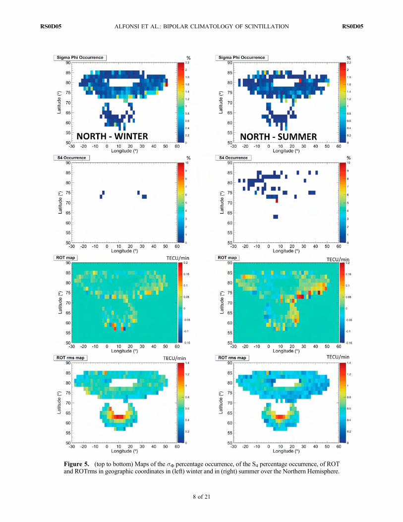
Figure 5. (top to bottom) Maps of the sΦ percentage occurrence, of the S4 percentage occurrence, of ROTand ROTrms in geographic coordinates in (left) winter and in (right) summer over the Northern Hemisphere.

ALFONSI ET AL.: BIPOLAR CLIMATOLOGY OF SCINTILLATION RS0D05RS0D05

8 of 21

Figure 6. Similar to Figure 5 over the Southern Hemisphere.

ALFONSI ET AL.: BIPOLAR CLIMATOLOGY OF SCINTILLATION RS0D05RS0D05

9 of 21

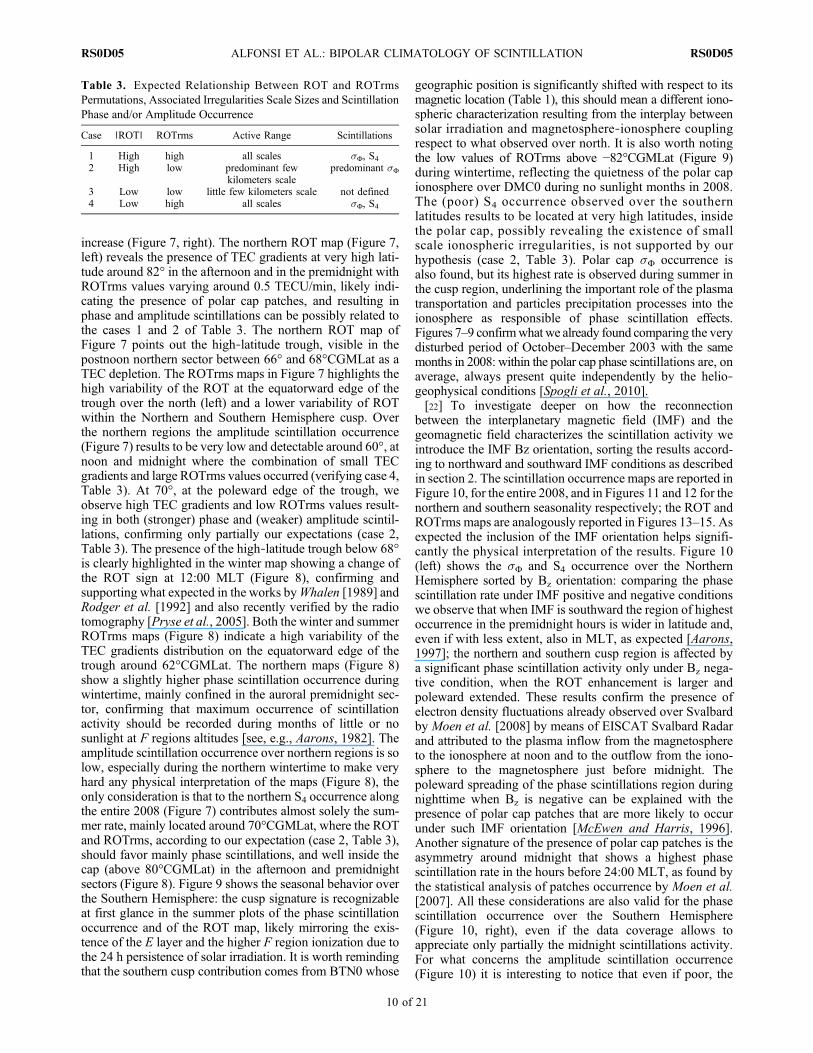
increase (Figure 7, right). The northern ROT map (Figure 7,left) reveals the presence of TEC gradients at very high lati-tude around 82° in the afternoon and in the premidnight withROTrms values varying around 0.5 TECU/min, likely indi-cating the presence of polar cap patches, and resulting inphase and amplitude scintillations can be possibly related tothe cases 1 and 2 of Table 3. The northern ROT map ofFigure 7 points out the high‐latitude trough, visible in thepostnoon northern sector between 66° and 68°CGMLat as aTEC depletion. The ROTrms maps in Figure 7 highlights thehigh variability of the ROT at the equatorward edge of thetrough over the north (left) and a lower variability of ROTwithin the Northern and Southern Hemisphere cusp. Overthe northern regions the amplitude scintillation occurrence(Figure 7) results to be very low and detectable around 60°, atnoon and midnight where the combination of small TECgradients and large ROTrms values occurred (verifying case 4,Table 3). At 70°, at the poleward edge of the trough, weobserve high TEC gradients and low ROTrms values result-ing in both (stronger) phase and (weaker) amplitude scintil-lations, confirming only partially our expectations (case 2,Table 3). The presence of the high‐latitude trough below 68°is clearly highlighted in the winter map showing a change ofthe ROT sign at 12:00 MLT (Figure 8), confirming andsupporting what expected in the works byWhalen [1989] andRodger et al. [1992] and also recently verified by the radiotomography [Pryse et al., 2005]. Both the winter and summerROTrms maps (Figure 8) indicate a high variability of theTEC gradients distribution on the equatorward edge of thetrough around 62°CGMLat. The northern maps (Figure 8)show a slightly higher phase scintillation occurrence duringwintertime, mainly confined in the auroral premidnight sec-tor, confirming that maximum occurrence of scintillationactivity should be recorded during months of little or nosunlight at F regions altitudes [see, e.g., Aarons, 1982]. Theamplitude scintillation occurrence over northern regions is solow, especially during the northern wintertime to make veryhard any physical interpretation of the maps (Figure 8), theonly consideration is that to the northern S4 occurrence alongthe entire 2008 (Figure 7) contributes almost solely the sum-mer rate, mainly located around 70°CGMLat, where the ROTand ROTrms, according to our expectation (case 2, Table 3),should favor mainly phase scintillations, and well inside thecap (above 80°CGMLat) in the afternoon and premidnightsectors (Figure 8). Figure 9 shows the seasonal behavior overthe Southern Hemisphere: the cusp signature is recognizableat first glance in the summer plots of the phase scintillationoccurrence and of the ROT map, likely mirroring the exis-tence of the E layer and the higher F region ionization due tothe 24 h persistence of solar irradiation. It is worth remindingthat the southern cusp contribution comes from BTN0 whose

geographic position is significantly shifted with respect to itsmagnetic location (Table 1), this should mean a different iono-spheric characterization resulting from the interplay betweensolar irradiation and magnetosphere‐ionosphere couplingrespect to what observed over north. It is also worth notingthe low values of ROTrms above −82°CGMLat (Figure 9)during wintertime, reflecting the quietness of the polar capionosphere over DMC0 during no sunlight months in 2008.The (poor) S4 occurrence observed over the southernlatitudes results to be located at very high latitudes, insidethe polar cap, possibly revealing the existence of smallscale ionospheric irregularities, is not supported by ourhypothesis (case 2, Table 3). Polar cap sΦ occurrence isalso found, but its highest rate is observed during summer inthe cusp region, underlining the important role of the plasmatransportation and particles precipitation processes into theionosphere as responsible of phase scintillation effects.Figures 7–9 confirmwhat we already found comparing the verydisturbed period of October–December 2003 with the samemonths in 2008: within the polar cap phase scintillations are, onaverage, always present quite independently by the helio‐geophysical conditions [Spogli et al., 2010].[22] To investigate deeper on how the reconnection

between the interplanetary magnetic field (IMF) and thegeomagnetic field characterizes the scintillation activity weintroduce the IMF Bz orientation, sorting the results accord-ing to northward and southward IMF conditions as describedin section 2. The scintillation occurrence maps are reported inFigure 10, for the entire 2008, and in Figures 11 and 12 for thenorthern and southern seasonality respectively; the ROT andROTrms maps are analogously reported in Figures 13–15. Asexpected the inclusion of the IMF orientation helps signifi-cantly the physical interpretation of the results. Figure 10(left) shows the sΦ and S4 occurrence over the NorthernHemisphere sorted by Bz orientation: comparing the phasescintillation rate under IMF positive and negative conditionswe observe that when IMF is southward the region of highestoccurrence in the premidnight hours is wider in latitude and,even if with less extent, also in MLT, as expected [Aarons,1997]; the northern and southern cusp region is affected bya significant phase scintillation activity only under Bz nega-tive condition, when the ROT enhancement is larger andpoleward extended. These results confirm the presence ofelectron density fluctuations already observed over Svalbardby Moen et al. [2008] by means of EISCAT Svalbard Radarand attributed to the plasma inflow from the magnetosphereto the ionosphere at noon and to the outflow from the iono-sphere to the magnetosphere just before midnight. Thepoleward spreading of the phase scintillations region duringnighttime when Bz is negative can be explained with thepresence of polar cap patches that are more likely to occurunder such IMF orientation [McEwen and Harris, 1996].Another signature of the presence of polar cap patches is theasymmetry around midnight that shows a highest phasescintillation rate in the hours before 24:00 MLT, as found bythe statistical analysis of patches occurrence by Moen et al.[2007]. All these considerations are also valid for the phasescintillation occurrence over the Southern Hemisphere(Figure 10, right), even if the data coverage allows toappreciate only partially the midnight scintillations activity.For what concerns the amplitude scintillation occurrence(Figure 10) it is interesting to notice that even if poor, the

Table 3. Expected Relationship Between ROT and ROTrmsPermutations, Associated Irregularities Scale Sizes and ScintillationPhase and/or Amplitude Occurrence

Case ∣ROT∣ ROTrms Active Range Scintillations

1 High high all scales sΦ, S42 High low predominant few

kilometers scalepredominant sΦ

3 Low low little few kilometers scale not defined4 Low high all scales sΦ, S4

ALFONSI ET AL.: BIPOLAR CLIMATOLOGY OF SCINTILLATION RS0D05RS0D05

10 of 21

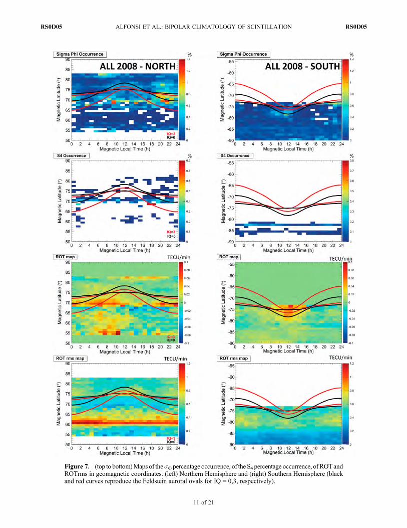
Figure 7. (top to bottom)Maps of thesΦ percentage occurrence, of the S4 percentage occurrence, ofROTandROTrms in geomagnetic coordinates. (left) Northern Hemisphere and (right) Southern Hemisphere (blackand red curves reproduce the Feldstein auroral ovals for IQ = 0,3, respectively).

ALFONSI ET AL.: BIPOLAR CLIMATOLOGY OF SCINTILLATION RS0D05RS0D05

11 of 21

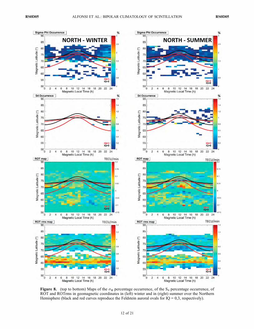
Figure 8. (top to bottom) Maps of the sΦ percentage occurrence, of the S4 percentage occurrence, ofROT and ROTrms in geomagnetic coordinates in (left) winter and in (right) summer over the NorthernHemisphere (black and red curves reproduce the Feldstein auroral ovals for IQ = 0,3, respectively).

ALFONSI ET AL.: BIPOLAR CLIMATOLOGY OF SCINTILLATION RS0D05RS0D05

12 of 21

Figure 9. Similar to Figure 8 over the Southern Hemisphere.

ALFONSI ET AL.: BIPOLAR CLIMATOLOGY OF SCINTILLATION RS0D05RS0D05

13 of 21

Figure 10. (top to bottom) Maps of the sΦ percentage occurrence, of the S4 percentage occurrence in geo-magnetic coordinates separating the IMF Bz positive and negative conditions. (left) Northern Hemisphereand (right) Southern Hemisphere (black and red curves reproduce the Feldstein auroral ovals for IQ = 0,3,respectively).

ALFONSI ET AL.: BIPOLAR CLIMATOLOGY OF SCINTILLATION RS0D05RS0D05

14 of 21

Figure 11. (top to bottom) Maps of the sΦ percentage occurrence and of the S4 percentage occurrence ingeomagnetic coordinates separating the IMF Bz positive and negative conditions in (left) winter and in(right) summer over the Northern Hemisphere (black and red curves reproduce the Feldstein auroral ovalsfor IQ = 0,3, respectively).

ALFONSI ET AL.: BIPOLAR CLIMATOLOGY OF SCINTILLATION RS0D05RS0D05

15 of 21

Figure 12. Similar to Figure 11 over the Southern Hemisphere.

ALFONSI ET AL.: BIPOLAR CLIMATOLOGY OF SCINTILLATION RS0D05RS0D05

16 of 21

Figure 13. (top to bottom) Maps of the ROT and ROTrms in geomagnetic coordinates separating the IMFBz positive and negative conditions over the (left) Northern Hemisphere and over the (right) SouthernHemisphere (black and red curves reproduce the Feldstein auroral ovals for IQ = 0,3, respectively).

ALFONSI ET AL.: BIPOLAR CLIMATOLOGY OF SCINTILLATION RS0D05RS0D05

17 of 21

Figure 14. (top to bottom) Maps of the ROT and ROTrms in geomagnetic coordinates separating the IMFBz positive and negative conditions over the Northern Hemisphere. (left) Winter and (right) summer (blackand red curves reproduce the Feldstein auroral ovals for IQ = 0,3, respectively).

ALFONSI ET AL.: BIPOLAR CLIMATOLOGY OF SCINTILLATION RS0D05RS0D05

18 of 21

Figure 15. Similar to Figure 14 over the Southern Hemisphere.

ALFONSI ET AL.: BIPOLAR CLIMATOLOGY OF SCINTILLATION RS0D05RS0D05

19 of 21

S4 climatology suggests that the regions more sensitive tohost small‐scale irregularities result to be the subauroral andauroral areas (visible in the northern maps) and the polar cap(visible in the northern and southern maps). Moreover, theobservations over both the hemispheres demonstrate that theamplitude scintillation within the cap is weakly dependent bythe Bz conditions. Over the northern regions (Figure 10, left)theMLT sector sensitive to subauroral amplitude scintillationchanges according to IMF orientation: when Bz is positive S4enhances around noon, while when Bz is negative S4 peaksaround noon and midnight. The cusp sector reveals to be veryeffective in producing phase scintillations, especially undersouthward IMF condition, and very ineffective in triggeringamplitude scintillations, independently by the IMF orien-tation. Our results indicate that, statistically under solarminimum, the presence of small‐scale irregularities (up tohundreds of meter) does not prevail in the cusp sector. Theassociation between high ROTrms and the spreading of ROTdistribution within the cusp could support such hypothesis:Figure 13 shows independently by the Bz sign and especiallyover the Southern Hemisphere, a low level of ROTrmsaround noon and an increase of ROT during the same hours.This could mean that at the cusp ionospheric irregularitiesat larger scales (ROT values correspond roughly to few/tenskilometers scales, see section 3), likely producing phasescintillations [Aarons, 1997], prevail to the ones at smallerscales (case 2, Table 3). The northern seasonality sorted byIMF orientation (Figure 11) shows a higher phase scintilla-tion in the winter premidnight auroral sector, particularlywhen Bz is negative. According to the homologous ROT andROTrmsmaps (Figure 14) in this region TEC gradients at fewkilometers scales are almost absent with low ROTrms asso-ciated values. From our hypothesis (case 3, Table 3) we arenot able to derive any explanation referred to the involvedirregularities scale sizes, so we can try to attribute the phasescintillation enhancement to the high plasma dynamics typi-cal of the southward IMF condition. Independently by theIMF orientation, we observe an absence of S4 occurrenceduring northern wintertime and a significant amplitudescintillation in summer, detectable especially at latitudesabove 70° during nighttime and afternoon hours and at about80° in the afternoon and pre midnight hours (Figure 11). Itshould indicate that in winter small‐scale irregularities in theNorthern Hemisphere are almost absent, while during sum-mer such irregularities could be present where we observeamplitude scintillation. Around 60° we observe, on average,that when an area shows the presence of intense gradients(high ROT) in coincidence with a lowering of ROTrms values(Figure 14) that area, independently by the season, is inef-fective in producing amplitude scintillations and effective inproducing phase scintillation (case 2, Table 3). Only theMLTdistribution of phase scintillation changes with the Bz sign(Figures 11 and 14). The southern seasonality (Figures 12and 15) shows clearly a significant ROT and ROTrmsenhancement in the cusp during summertime, that, under Bz

negative condition is even more extended in MLT. Asguessed in Table 3 (case 1), high ∣ROT∣ and ROTrms shouldactivate irregularities at all scale sizes. From our results, onlysΦ occurrence increases during summer (Figure 12), possiblyconfirming what found by Vickrey and Kelley [1982] andmore recently discussed by Kivanc and Heelis [1997]: during

summer is present a conducting E region whose effect is toshort out the electric fields followed by the increased ionsdiffusion across the magnetic field. Such conditions wouldproduce a significantly bigger loss of irregularities intensitiesat smaller scales compared to those at larger scales resultingin steepening of the irregularity spectra. Inside the polarcap above −80° both ∣ROT∣ and ROTrms are low, and S4occurrence shows up perhaps indicating the presence ofirregularities at smaller scales; polar cap phase scintillation,as expected, results to be produced by a variety of irregular-ities sizes. Figure 13 shows how the ROTrms within thepolar cap is IMF independent.

5. Summary and Conclusions

[23] Our work deals with the scintillation and TEC clima-tology, termed GBSC, derived from a high‐latitude networkof receivers acquiring 50 Hz amplitude and phase data fromthe GPS satellites constellation. The network consists of fourreceivers in the Northern Hemisphere and two in the southernone that does not allow a conjugated study of the scintillationoccurrence, but that permits an investigation mainly basedon the very different coverage. The northern array allowsthe observation of subauroral, auroral, cusp and cap sectors,while the southern array covers essentially the cusp and capregions. The climatology has been derived using the mea-surements collected during 2008, a period of very quiet helio‐geophysical conditions. Our climatology assesses the Rate OfTEC (ROT) scenario on irregularities scales of few to tens ofkilometers and its related distribution by means of ROTrmsmapping. As on L band the probing size is of the order ofhundreds of meters, the ROT and ROTrms mapping shouldprovide information on intensity and distribution of largerscale irregularities. In particular high ROTrms values wouldsuggest the presence of other scale sizes, possibly includingthe smaller ones.[24] The achievements of our study here presented have to

be considered as preliminary but present promising potenti-alities for the future development of forecasting algorithms aswell as for testing irregularities and scintillation models, suchas: WBMOD [Secan et al., 1997, and references therein],or WAM [Wernik et al., 2007].[25] The major results can be summarized as follows:[26] 1. At high latitudes, on average under low solar activ-

ity, scintillation is more likely to occur on the phase than onthe amplitude of the received signal.[27] 2. Different combinations of ROT and ROTrms

changes result in different scintillation scenarios: from ourhypothesis, generally verified by the results, high level of∣ROT∣ and ROTrms results in amplitude and phase scintil-lations; high level of ∣ROT∣ and low ROTrms values favorphase scintillations; low level of ∣ROT∣ and high ROTrmsvalues results in amplitude and phase scintillations.[28] 3. Cusp sector results to be very effective in causing

phase scintillations and almost ineffective in giving ampli-tude scintillations.[29] 4. Polar cap patches can cause phase and amplitude

scintillations.[30] 5. The seasonal variability is observed mainly over the

cusp, where the E layer appearance likely results in a ROTenhancement in the noon sector.

ALFONSI ET AL.: BIPOLAR CLIMATOLOGY OF SCINTILLATION RS0D05RS0D05

20 of 21

[31] 6. The IMF orientation influences mainly the scintil-lations distribution in magnetic local time, highlighting theimportant role of the plasma inflow and outflow from and tothe magnetosphere in the noon and midnight hours.

[32] Acknowledgments. Authors thank the Programma Nazionale diRicerche in Antartide (PNRA), CNR (Consiglio Nazionale delle Ricerche),the Physical Sciences Research Council of the UK (EPSRC) and the RoyalSociety. The authors also thank the National Space Science Data Center(NSSDC) for the software calculating the auroral oval position, the modelauthors, Holzworth and Meng, and NASA for the ACE data.

ReferencesAarons, J. (1982), Global morphology of ionospheric scintillation, Proc.IEEE, 70, 360–378, doi:10.1109/PROC.1982.12314.

Aarons, J. (1993), The longitudinal morphology of equatorial F‐layerirregularities relevant to their occurrence, Space Sci. Rev., 63, 209–243,doi:10.1007/BF00750769.

Aarons, J. (1997), Global Positioning System phase fluctuations at aurorallatitudes, J. Geophys. Res., 102(A8), 17,219–17,231, doi:10.1029/97JA01118.

Baker, K. B., and S. Wing (1989), A new magnetic coordinate system forconjugate studies at high latitudes, J. Geophys. Res., 94, 9139–9143,doi:10.1029/JA094iA07p09139.

Basu, S., K. M. Groves, J. M. Quinn, and P. Doherty (1999), A comparisonof TEC fluctuations and scintillations at Ascension Island, J. Atmos. Sol.Terr. Phys., 61(16), 1219–1226, doi:10.1016/S1364-6826(99)00052-8.

Basu, Su., and S. Basu (1985), Equatorial scintillations: Advances sinceISEA‐6, J. Atmos. Terr. Phys., 47, 753–768, doi:10.1016/0021-9169(85)90052-2.

Coco, D. S., T. L. Gaussiran, and C. Coker (1995), Passive detection ofsporadic E using GPS phase measurements, Radio Sci., 30, 1869–1874,doi:10.1029/95RS02453.

Feldstein, Y. I. (1963), On morphology and auroral and magnetic distur-bances at high latitudes, Geomagn. Aeron., 3, 138.

Forte, B., and S. M. Radicella (2002), Problems in data treatment for iono-spheric scintillation measurements, Radio Sci., 37(6), 1096, doi:10.1029/2001RS002508.

Foster, J. C., et al. (2005), Multiradar observations of the polar tongue ofionization, J. Geophys. Res., 110, A09S31, doi:10.1029/2004JA010928.

Holzworth, R. H., and C.‐I. Meng (1975), Mathematical representationof the auroral oval, Geophys. Res. Lett., 2, 377–380, doi:10.1029/GL002i009p00377.

Hunsucker, R. D., and J. K. Hargreaves (2003), The High‐Latitude Iono-sphere and Its Effects on Radio Propagation, 1st ed., Cambridge Univ.Press, Cambridge, U. K.

Jayachandran, P. T., J. W. MacDougall, E. F. Donovan, J. M. Ruohoniemi,K. Liou, D. R. Moorcroft, and J.‐P. St‐Maurice (2003), Substorm asso-ciated changes in the high‐latitude ionospheric convection, Geophys.Res. Lett., 30(20), 2064, doi:10.1029/2003GL017497.

Kersley, L., S. E. Pryse, and N. S. Wheadon (1988), Amplitude and phasescintillation at high latitudes over northern Europe, Radio Sci., 23,320–330, doi:10.1029/RS023i003p00320.

Kivanc, O., and R. A. Heelis (1997), Structures in ionospheric numberdensity and velocity associated with polar cap ionization patches,J. Geophys. Res., 102, 307–318, doi:10.1029/96JA03141.

Li, G., B. Ning, Z. Ren, and L. Hu (2010), Statistics of GPS ionosphericscintillation and irregularities over polar regions at solar minimum,GPS Solut., 14, 331–341, doi:10.1007/s10291-009-0156-x.

MacDougall, J. W. (1990a), Distribution of irregularities in the northernpolar region determined from HILAT observations, Radio Sci., 25,115–124, doi:10.1029/RS025i002p00115.

MacDougall, J. W. (1990b), The polar‐cap scintillation zone, J. Geomag.Geoelectr., 42, 777–788.

Mannucci, A. J., B. D. Wilson, and C. D. Edwards (1993), A new methodfor monitoring the Earth ionosphere total electron content using the GPSglobal network, paper presented at ION GPS‐93, Inst. of Navig., SaltLake City, Utah.

McComas, D. J., S. J. Bame, P. Barker, W. C. Feldman, J. L. Phillips,P. Riley, and J. W. Griffee (1998), Solar Wind Electron Proton AlphaMonitor (SWEPAM) for the Advanced Composition Explorer, SpaceSci. Rev., 86(1), 563–612.

McEwen, D. J., and D. P. Harris (1996), Occurrence patterns of F layerpatches over the north magnetic pole, Radio Sci., 31(3), 619–628,doi:10.1029/96RS00312.

Moen, J., N. Gulbrandsen, D. A. Lorentzen, and H. C. Carlson (2007), Onthe MLT distribution of F region polar cap patches at night, Geophys.Res. Lett., 34, L14113, doi:10.1029/2007GL029632.

Moen, J., X. C. Qiu, H. C. Carlson, R. Fujii, and I. W. McCrea (2008), Onthe diurnal variability in F2‐region plasma density above the EISCATSvalbard radar, Ann. Geophys., 26, 2427–2433, doi:10.5194/angeo-26-2427-2008.

Pryse, S. E., K. L. Dewis, R. L. Balthazor, H. R. Middleton, and M. H.Denton (2005), The dayside high‐latitude trough under quiet geomag-netic conditions: Radio tomography and the CTIP model, Ann. Geophys.,23, 1199–1206, doi:10.5194/angeo-23-1199-2005.

Pryse, S. E., L. Kersley, D. Malan, and G. J. Bishop (2006), Parameteriza-tion of the main ionospheric trough in the European sector, Radio Sci.,41, RS5S14, doi:10.1029/2005RS003364.

Rino, C. L. (1979a), A power law phase screen model for ionosphericscintillation: 1. Weak scatter, Radio Sci., 14(6), 1135–1145.

Rino, C. L. (1979b), A power law phase screen model for ionosphericscintillation: 2. Strong scatter, Radio Sci., 14(6), 1147–1155.

Rodger, A. S., and J. Smith (1989), Antarctic studies of the coupledionosphere‐magnetosphere system, Philos. Trans. R. Soc. London, Ser. A,328, 271–287, doi:10.1098/rsta.1989.0036.

Rodger, A. S., R. J. Moffett, and S. Quegan (1992), The role of ion driftin the formation of ionisation troughs in the mid‐ and high‐latitudeionosphere—A review, J. Atmos. Terr. Phys., 54(1), 1–30, doi:10.1016/0021-9169(92)90082-V.

Ruohoniemi, J. M., and R. A. Greenwald (2005), Dependencies of high‐latitude plasma convection: Consideration of interplanetary magneticfield, seasonal and universal time factors in statistical patterns, J. Geophys.Res., 110, A09204, doi:10.1029/2004JA010815.

Secan, J. A., R. M. Bussey, E. J. Fremouw, and S. Basu (1997), High‐latitude upgrade to the Wideband ionospheric scintillation model, RadioSci., 32, 1567–1574, doi:10.1029/97RS00453.

Smith, C. W., J. L’Heureux, N. F. Ness, M. H. Acuña, L. F. Burlaga, andJ. Scheifele (1998), The ACE Magnetic Fields Experiment, Space Sci.Rev., 86(1), 613–632.

Spogli, L., L. Alfonsi, G. De Franceschi, V. Romano, M. H. O. Aquino,and A. Dodson (2009), Climatology of GPS ionospheric scintillationsover high and mid‐latitude European regions, Ann. Geophys., 27,3429–3437, doi:10.5194/angeo-27-3429-2009.

Spogli, L., L. Alfonsi, G. De Franceschi, V. Romano, M. H. O. Aquino,and A. Dodson (2010), Climatology of GNSS ionospheric scintillationat high and mid latitudes under different solar activity conditions, NuovoCimento B, doi:10.1393/ncb/i2010-10857-7.

Taylor, J. R. (1997), An Introduction to Error Analysis: The Study ofUncertainties in Physical Measurement, 2nd ed., Univ. Sci., Sausalito,Calif.

Van Dierendonck, A. J., J. Klobuchar, and Q. Hua (1993), Ionosphericscintillation monitoring using commercial single frequency C/A codereceivers, paper presented at the Sixth International Technical Meeting(ION GPS‐93), Satell. Div., Inst. of Navig., Salt Lake City, Utah,22–24 Sept.

Vickrey, J. F., and M. C. Kelley (1982), The effects of a conducting E layeron classical F region cross‐field plasma diffusion, J. Geophys. Res., 87,4461–4468, doi:10.1029/JA087iA06p04461.

Webb, D. F., and J. H. Allen (2004), Spacecraft and ground anomaliesrelated to the October‐November 2003 solar activity, Space Weather,2, S03008, doi:10.1029/2004SW000075.

Wernik, A. W., L. Alfonsi, and M. Materassi (2007), Scintillation modellingusing in‐situ data, Radio Sci., 42, RS1002, doi:10.1029/2006RS003512.

Whalen, J. A. (1989), The daytime F layer trough and its relationto ionospheric‐magnetospheric convection, J. Geophys. Res., 94,17,169–17,184.

L. Alfonsi, G. De Franceschi, V. Romano, and L. Spogli, IstitutoNazionale di Geofisica e Vulcanologia, Via di Vigna Murata 605,I‐00143 Rome, Italy.M. Aquino and A. Dodson, Institute of Engineering Surveying and Space

Geodesy, University of Nottingham, Triumph Road, Nottingham NG72TU, UK.C. N. Mitchell, Department of Electronic and Electrical Engineering,

University of Bath, Bath BA2 7AY, UK.

ALFONSI ET AL.: BIPOLAR CLIMATOLOGY OF SCINTILLATION RS0D05RS0D05

21 of 21