Travelling ionospheric disturbance over California mid 2000

Nonlinear Processes in Geophysics, 13, 1–7, 2006SRef-ID: 1607-7946/npg/2006-13-1European Geosciences Union© 2006 Author(s). This work is licensedunder a Creative Commons License.

Nonlinear Processesin Geophysics

Travelling ionospheric disturbance over California mid 2000

M. Hawarey

Purdue University, West Lafayette, Indiana, USA

Received: 12 July 2005 – Revised: 16 November 2005 – Accepted: 16 November 2005 – Published: 16 January 2006

Part of Special Issue “Turbulent transport in geosciences”

Abstract. In this paper, the GPS data collected by more than130 permanent GPS stations that belong to the Southern Cal-ifornia Integrated GPS Network (SCIGN) around the launchof a Minuteman-II missile on 8 July 2000 (UTC) is processedto reveal traveling ionospheric disturbance (TID) all over thenetwork on average 15 min after the launch. This TID wasinitially perceived to be excited by the launch itself, but thisconclusion is challenged by the propagation direction. Thisis because this TID seems to travel towards the air force basefrom where the launch took place, not far away from it. Thischallenge is based on the assumption that TID is occurringat one single ionospheric altitude. While the nature of iono-sphere supports such horizontally-guided propagation, multi-altitude ionospheric pierce points are hypothesized, whichwould support the suggestion that detected TID is excitedby the missile launch itself, despite the apparent reverse di-rection of propagation. The overall analysis rules out anyextra-terrestrial sources like solar flares, or seismic sourceslike earthquakes, which confirms the conclusion of TID exci-tation by the launch. There is apparent coherence of the TIDfor about 45 min and the propagation speed of TID within thelayer of ionosphere is calculated to be approximately equal to1230 m/s. While the usual assumption for TID is that they oc-cur around an altitude of 350 km, such sound speed can onlyoccur at much higher altitudes. Further research is recom-mended to accurately pinpoint the ionospheric pierce pointsand develop an algorithm to locate the source of TID in caseit is totally unknown.

1 Introduction

Observations collected by dual-frequency GPS receivershave proven to be efficient in calculating absolute TotalElectron Content (TEC) along the paths of incoming sig-nals, thus enabling the mapping of the ionosphere and the

Correspondence to:M. Hawarey([email protected])

identification of disturbance in the density of TEC. Usingthis GPS-assisted methodology, traveling ionospheric distur-bance (TID) excited by earthquakes (e.g. Afraimovich et al.,2001; Hawarey, 2002; Hawarey and Ayan, 2004), rocketlaunches (e.g. Afraimovich et al., 2000) and other sourceshave been reported. Researchers with no thorough back-ground are advised to refer to Beach et al. (1997), Fitzger-ald (1997), Ho et al. (1996), Matsunaga et al. (2003), Pi etal. (1997), Saito et al. (1998), Warnant and Pottiaux (2000).Although dual-frequency GPS observations provide an easytool to calculate absolute values of TEC, this information isredundant for the mere purpose of investigating TID and anybias in the TEC values would not influence the algorithm.

In this paper the data collected by more than 130 SCIGNstations are processed to show this network’s, and thus anysimilar dense GPS network’s capability to identify and an-alyze TID over a big geographical region, and to determinethe direction and speed of the propagation of TID.

2 Algorithm

For a detailed mathematical formulation, the reader is kindlyreferred to Hawarey and Ayan (2005). On the other hand, theredundancy of absolute TEC values for this particular appli-cation of TID detection is emphasized herewith. The onlyformula deemed necessary is:

TECb =(L1f2 − L2f1)

f1

λ2

40.3

(f 21 f 2

2 )

(f 22 − f 2

1 )(1)

where the subscriptb indicates biased TEC values, L1 andL2 are phase observations provided in RINEX files, f1 andf2 are the famous GPS frequencies (i.e. f1=1575.42 MHzand f2=1227.60 MHz), andλ2 is the wavelength of f2(i.e. 24.42 cm).

In order to detect TID in the raw time series provided byEq. (1), various filters need to be tested (i.e. low-pass, high-pass, and band-pass) with various cut-off values, to makesure all types of potential TID are covered. Decision was

2 M. Hawarey: Travelling ionospheric disturbance over California mid 2000

11

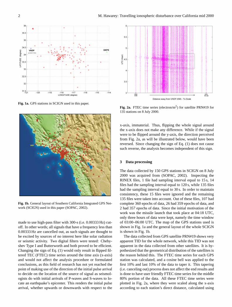
Figure 1a. GPS stations in SCIGN used in this paper. Fig. 1a. GPS stations in SCIGN used in this paper.

12

Figure 1b. General layout of Southern California Integrated GPS Network (SCIGN) used in

this paper (SOPAC, 2002).

Fig. 1b. General layout of Southern California Integrated GPS Net-work (SCIGN) used in this paper (SOPAC, 2002).

made to use high-pass filter with 300-s (i.e. 0.00333 Hz) cut-off. In other words; all signals that have a frequency less than0.00333 Hz are cancelled out, as such signals are thought tobe excited by sources of no interest here like solar radiationor seismic activity. Two digital filters were tested: Cheby-shev Type I and Butterworth and both proved to be efficient.Changing the sign of Eq. (1) would only result in flipped fil-tered TEC (FTEC) time series around the time axis (x-axis)and would not affect the analysis procedure or formulatedconclusions, as this field of research has not yet reached thepoint of making use of the direction of the initial pulse arrivalto decide on the location of the source of signal as seismol-ogists do with initial arrivals of P-waves and S-waves to lo-cate an earthquake’s epicenter. This renders the initial pulsearrival, whether upwards or downwards with respect to the

13

Figure 2a: FTEC time series (electron/meter^2) for satellite PRN#19 for 135 stations on 8

July 2000.

Fig. 2a. FTEC time series (electron/m2) for satellite PRN#19 for135 stations on 8 July 2000.

x-axis, immaterial. Thus, flipping the whole signal aroundthe x-axis does not make any difference. While if the signalwere to be flipped around the y-axis, the direction perceivedfrom Fig. 2a, as will be illustrated below, would have beenreversed. Since changing the sign of Eq. (1) does not causesuch reverse, the analysis becomes independent of this sign.

3 Data processing

The data collected by 150 GPS stations in SCIGN on 8 July2000 was acquired from (SOPAC, 2002). Inspecting theRINEX files, 1 file had sampling interval equal to 15 s, 14files had the sampling interval equal to 120 s, while 135 fileshad the sampling interval equal to 30 s. In order to maintainconsistency, these 15 files were ignored and the remaining135 files were taken into account. Out of these files, 107 hadcomplete 360 epochs of data, 26 had 359 epochs of data, and2 had 357 epochs of data. Since the initial motivation of thework was the missile launch that took place at 04:18 UTC,only three hours of data were kept, namely the time windowof 03:00–06:00 UTC. The map of the GPS stations used isshown in Fig. 1a and the general layout of the whole SCIGNis shown in Fig. 1b.

The data collected from GPS satellite PRN#19 shows veryapparent TID for the whole network, while this TID was notapparent in the data collected from other satellites. It is hy-pothesized that the geometrical distribution of the satellites isthe reason behind this. The FTEC time series for each GPSstation was calculated, and a cosine bell was applied to thefirst 10% and last 10% of the data to taper it. This tapering(i.e. canceling out) process does not affect the end results andis done to have user friendly FTEC time series for the middle80% portion of the data. All these FTEC time series wereplotted in Fig. 2a, where they were scaled along the x-axisaccording to each station’s direct distance, calculated using

M. Hawarey: Travelling ionospheric disturbance over California mid 2000 3

14

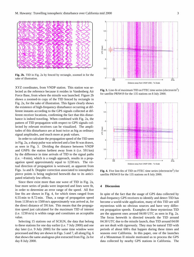
Figure 2b: TID in figure 2a by fenced by rectangle, zoomed in for the sake of illustration. Fig. 2b. TID in Fig. 2a by fenced by rectangle, zoomed in for thesake of illustration.

XYZ coordinates, from VNDP station. This station was se-lected as the reference because it resides in Vandenberg AirForce Base, from where the missile was launched. Figure 2bshows a zoomed-in copy of the TID fenced by rectangle inFig. 2a, for the sake of illustration. This figure clearly showsthe existence of high-frequency disturbance occurring at dif-ferent instants according to the GPS signals collected at dif-ferent receiver locations, confirming the fact that this distur-bance is indeed traveling. When combined with Fig. 2a, thepattern of TID propagation with respect to GPS signals col-lected by relevant receivers can be visualized. The ampli-tudes of this disturbance are at least twice as big as ordinarysignal amplitudes, and much more at peak values.

In order to calculate the propagation speed of the TID seenin Fig. 2a, a sharp pulse was selected and a line fit was drawn,as seen in Fig. 3. Dividing the distance between VNDPand GNPS: the station farthest away from it (i.e. 591 km)by the difference in time arrivals of TID to the signal paths(i.e. ∼8 min), which is a rough approach, results in a prop-agation speed approximately equal to 1230 m/s. The vir-tual direction of propagation is westward, as apparent fromFigs. 1a and b. Doppler correction associated to ionosphericpierce points is being neglected herewith due to its antici-pated relatively low effects.

Since there exist more than one wave of TID in Fig. 2a,four more series of peaks were inspected and lines were fit,in order to determine an error range of the speed. All fiveline fits are shown in Fig. 4, for which times ranged from6.55 min to 8.72 min. Thus, a range of propagation speedfrom 1130 m/s to 1500 m/s approximately was arrived at, forthe direct distance of 591 km. This means that the propaga-tion speed just calculated for the maximum TID of interest(i.e. 1230 m/s) is within range and constitutes an acceptablevalue.

Selecting 15 stations out of SCIGN, the data that belongto these stations for one day earlier (i.e. 7 July 2000) and oneday later (i.e. 9 July 2000) for the same time window wereprocessed and they are shown in Figs. 5 and 7, all along Fig. 6that shows the same analogous plot extracted from Fig. 2a forday 8 July 2000.

15

Figure 3: Line-fit of maximum TID on FTEC time series (electron/meter^2) for satellite

PRN#19 for the 135 stations on 8 July 2000.

Fig. 3. Line-fit of maximum TID on FTEC time series (electron/m2)for satellite PRN#19 for the 135 stations on 8 July 2000.

16

Figure 4: Five line-fits of TID on FTEC time series (electron/meter^2) for satellite PRN#19

for the 135 stations on 8 July 2000.

Fig. 4. Five line-fits of TID on FTEC time series (electron/m2) forsatellite PRN#19 for the 135 stations on 8 July 2000.

4 Discussion

In spite of the fact that the usage of GPS data collected bydual-frequency GPS receivers to identify and detect TID hasbecome a world-wide application, many of this TID are stillmysterious with no obvious sources and have very differ-ent propagation speeds. Examples of these mysterious TIDare the apparent ones around 04:00 UTC as seen in Fig. 2a.The focus herewith is directed towards the TID around04:30 UTC due to the missile launch, thus TID around 04:00are not dealt with rigorously. They may be natural TID withperiods of about 600 s that happen during these times andseasons over California. In this paper, one of the launchesof a Minuteman II missile motivated us to process the GPSdata collected by nearby GPS stations in California. The


17

Figure 5: FTEC time series (electron/meter^2) for satellite PRN#19 for 15 selected stations on

7 July 2000.

Fig. 5. FTEC time series (electron/m2) for satellite PRN#19 for 15selected stations on 7 July 2000.

18


8 July 2000.


initial perception indicated the detection of TID excited bythis launch, with TID showing peak values around 15 min af-ter the launch, as the missile launch took place at 04:18 UTCand the initial strikes of pulse (the series of peaks), as seenin Fig. 2a, occured from 04:26 UTC thru 04:35 UTC. Af-ter inspection of the density of peaks, 04:33 o’clock wastaken as an average; 15 min after 04:18 UTC. This wouldindicate a propagation speed from the launch pad towardsthe IPs (Ionospheric Points: points of intersection betweenGPS signal rays and ionospheric layer with maximum elec-tron density, often called ionospheric pierce points) equiva-lent to sound speeds. Taking 300 km as the approximate alti-tude at which IPs occurred, an average value of propagationspeed of TID from the launch pad towards IPs was calculatedapproximately equal to 334 m/s. While other altitude values

19


9 July 2000.


Fig. 8. Orbit of satellite PRN#19 over SCIGN on 8 July 2000.

could have been selected (Hawarey et al., 2005), this value isdeemed appropriate to get a good impression and idea of howthe disturbance is traveling. Processing few stations’ datarendered the acquired propagation speed sensible. However,as the results have been acquired for 135 stations, the virtualVNDPward propagation direction suggests that the detectedTID perhaps have not been excited by the launch. The prop-agation speed calculated from Fig. 3 (i.e. 1230 m/s) suggestsa higher value than the one calculated assuming excitationby the launch (i.e. 334 m/s). On the other hand, it must bekept in mind that the value of 1230 m/s is an approximation,in the presence of other waves as seen in Fig. 4. Also, the1230 m/s is a propagation speed within the ionosphere itself,while 334 m/s is a propagation speed within the lower atmo-spheric layers towards the ionosphere. This point deservesfurther inspection, thus further research is recommended.

It should be noticed that despite the calculation of propa-gation speed from Fig. 3 being approximate; the position of


21

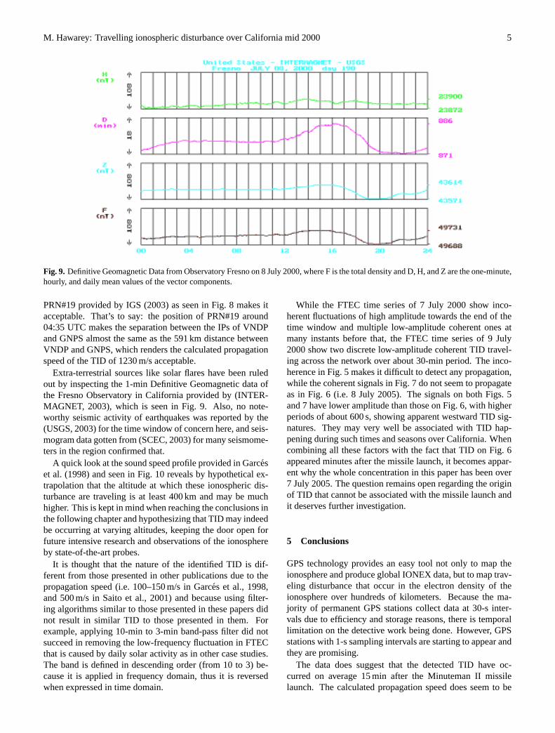
Figure 9: Definitive Geomagnetic Data from Observatory Fresno on 8 July 2000, where F is

the total density and D, H, and Z are the one-minute, hourly, and daily mean values of the

vector components.

Fig. 9. Definitive Geomagnetic Data from Observatory Fresno on 8 July 2000, where F is the total density and D, H, and Z are the one-minute,hourly, and daily mean values of the vector components.

PRN#19 provided by IGS (2003) as seen in Fig. 8 makes itacceptable. That’s to say: the position of PRN#19 around04:35 UTC makes the separation between the IPs of VNDPand GNPS almost the same as the 591 km distance betweenVNDP and GNPS, which renders the calculated propagationspeed of the TID of 1230 m/s acceptable.

Extra-terrestrial sources like solar flares have been ruledout by inspecting the 1-min Definitive Geomagnetic data ofthe Fresno Observatory in California provided by (INTER-MAGNET, 2003), which is seen in Fig. 9. Also, no note-worthy seismic activity of earthquakes was reported by the(USGS, 2003) for the time window of concern here, and seis-mogram data gotten from (SCEC, 2003) for many seismome-ters in the region confirmed that.

A quick look at the sound speed profile provided in Garceset al. (1998) and seen in Fig. 10 reveals by hypothetical ex-trapolation that the altitude at which these ionospheric dis-turbance are traveling is at least 400 km and may be muchhigher. This is kept in mind when reaching the conclusions inthe following chapter and hypothesizing that TID may indeedbe occurring at varying altitudes, keeping the door open forfuture intensive research and observations of the ionosphereby state-of-the-art probes.

It is thought that the nature of the identified TID is dif-ferent from those presented in other publications due to thepropagation speed (i.e. 100–150 m/s in Garces et al., 1998,and 500 m/s in Saito et al., 2001) and because using filter-ing algorithms similar to those presented in these papers didnot result in similar TID to those presented in them. Forexample, applying 10-min to 3-min band-pass filter did notsucceed in removing the low-frequency fluctuation in FTECthat is caused by daily solar activity as in other case studies.The band is defined in descending order (from 10 to 3) be-cause it is applied in frequency domain, thus it is reversedwhen expressed in time domain.

While the FTEC time series of 7 July 2000 show inco-herent fluctuations of high amplitude towards the end of thetime window and multiple low-amplitude coherent ones atmany instants before that, the FTEC time series of 9 July2000 show two discrete low-amplitude coherent TID travel-ing across the network over about 30-min period. The inco-herence in Fig. 5 makes it difficult to detect any propagation,while the coherent signals in Fig. 7 do not seem to propagateas in Fig. 6 (i.e. 8 July 2005). The signals on both Figs. 5and 7 have lower amplitude than those on Fig. 6, with higherperiods of about 600 s, showing apparent westward TID sig-natures. They may very well be associated with TID hap-pening during such times and seasons over California. Whencombining all these factors with the fact that TID on Fig. 6appeared minutes after the missile launch, it becomes appar-ent why the whole concentration in this paper has been over7 July 2005. The question remains open regarding the originof TID that cannot be associated with the missile launch andit deserves further investigation.

5 Conclusions

GPS technology provides an easy tool not only to map theionosphere and produce global IONEX data, but to map trav-eling disturbance that occur in the electron density of theionosphere over hundreds of kilometers. Because the ma-jority of permanent GPS stations collect data at 30-s inter-vals due to efficiency and storage reasons, there is temporallimitation on the detective work being done. However, GPSstations with 1-s sampling intervals are starting to appear andthey are promising.

The data does suggest that the detected TID have oc-curred on average 15 min after the Minuteman II missilelaunch. The calculated propagation speed does seem to be


Fig. 10.Sound speed profile up to 200 km altitude in the atmosphere(Garces et al., 1998).

consistent with the overall phenomena, too. The major chal-lenge against such conclusion of launch detection would risefrom the apparent westward direction of propagation, whichis somehow similar to Afraimovich et al. (2003), where itwas stated that the TID that occurred after high-altitude ex-plosion had a propagation direction not supporting the hy-pothesis that the explosion had excited them. Such a chal-lenge is based on the assumption that the entire ionosphericdisturbance took place at the same altitude. While the natureof the layer of ionosphere may support such horizontally-guided propagation, it certainly does not exclude the varying-altitude propagation, thus the challenge is arguable. Actually,if it is hypothesized to have high-altitude pierce points nearthe launch pad and low-altitude pierce points faraway fromit, in the absence of tangible evidence that proves the im-possibility of this hypothesis, then westward direction wouldbe acceptable for TID excited by the missile launch. In theabsence of any other source that may have excited the TID,like solar flares or seismic activity, the conclusion of mis-sile launch detection is strengthened. This leads us to con-clude, at the same time, the potential capability of pinpoint-ing the location of the source (i.e. launch pad in this case)using GPS data. Further research and full geophysical anal-ysis is deemed necessary to try to decide on the exact piercepoints’ locations and to develop an algorithm to pinpoint thesource, in case it is unknown. Such research would show ifthere are relationships among TID occurring after the missilelaunch and those appearing one day before and one day after,which are thought in this paper to be associated with seasonalTID over California during such times.

The varying values of propagation speeds reported in theliterature and in this paper indicate the existence of differenttypes of disturbances traveling across the ionosphere withdifferent speeds and at different heights. Further extensiveresearch is recommended to classify the different types ofTID and to develop a standard documentation format forthem (e.g. TIDEX).

Acknowledgements.The author would like to thank everyone as-sisting in having the websites of Scripps Orbit and Permanent ArrayCenter (SOPAC), International GPS Service (IGS), United StatesGeological Survey (USGS) and Southern California EarthquakeData Center (SCEC) fully functional and available to the usageof everyone world-wide, free of charge. Also, INTERMAGNETis acknowledged for providing the complete sets of DefinitiveGeomagnetic Data, free of charge.

Edited by: J. M. RedondoReviewed by: H. Schuh and two other referees

References

Afraimovich, E. L., Kosogorov, E. A., Palamarchouk, K. S.,Perevalova, N. P., and Plotnikov, A. V.: The use of GPS arraysin detecting the ionospheric response during rocket launchings,Earth, Planets, and Space, 52, N11, 1061–1066, 2000.

Afraimovich, E. L., Perevalova, N. P., Plotnikov, A. V. and Uralov,A. M.: The shock-acoustic waves generated by the earthquakes,Ann. Geophys., 19, 395–409, 2001,SRef-ID: 1432-0576/ag/2001-19-395.

Afraimovich, E. L., Voyeikov, S. V., Lesyuta, O. S., Perevalova,N. P., and Nagorsky, P. M.: The traveling ionospheric distur-bance conceivably initiated by a high altitude explosion duringthe testing of the US anti-missile system on July 15, 2001, Solar-Terrestrial Physics, 3, Institute of Solar-Terrestrial Physics SBRAS, Irkutsk, 73–79, 2003.

Beach, T. L., Kelley, M. C., and Kintner, P. M.: Total electron con-tent variations due to nonclassical traveling ionospheric distur-bances: Theory and Global Positioning System observations, J.Geophys. Res., 102, 7279–7292, 1997.

Fitzgerald, T. J.: Observations of total electron content perturba-tions on GPS signals caused by a ground level explosion, J. At-mos. Terr. Phys., 59, 829–834, 1997.

Garces, M. A., Hansen, R. A., and Lindquist, K. G.: Trav-eltimes for infrasonic waves propagating in a stratified at-mosphere, Geophys. J. Int., 135(1), 255, doi:10.1046/j.1365-246X.1998.00618.x, 1998.

Hawarey, M.: GPS Detection of Izmit Earthquake and Shape Modelof already GPS-Detected Space Shuttle Launch in 1993, WeikkoA. Heiskanen Symposium in Geodesy, The Ohio State Univer-sity, 1–4 October 2002.

Hawarey, M. and Ayan, T.: GPS detection of ionospheric pertur-bations excited by space shuttle ascent, earthquake, and missilelaunch, itudergisi, Ser. d, 3, No. 2-3-4-5, ISSN 1303-703X, 45–56, 2004.

Hawarey, M. and Ayan, T.: GPS Detection of Minuteman II Launchand Positioning of Launch Site, J. Surveying Eng., 131, 3, 78–86,doi:10.1061/(ASCE)0733-9453(2005)131:3(78), 2005.

Hawarey, M., Hobiger, T., and Schuh, H.: Effects of the 2nd orderionospheric terms on VLBI measurements, Geophys. Res. Lett.,32(11), L11304, doi:10.1029/2005GL022729, 2005.

http://direct.sref.org/1432-0576/ag/2001-19-395


Ho, C. M., Mannucci, A. J., Lindqwister, U. J., Pi, X., and Tsuru-tani, B. T.: Global ionosphere perturbations monitored by theworldwide GPS network, Geophys. Res. Lett., 23(22), 3219–3222, 1996.

INTERMAGNET: International Real-time Magnetic ObservatoryNetwork, CD of Definitive Geomagnetic Data of 2000, France,2003.

IGS: International GPS Service’s website:http://igscb.jpl.nasa.gov/index.html, 2003.

Matsunaga, K., Hoshinoo, K., and Igarashi, K.: Observations ofIonospheric Scintillation on GPS Signals in Japan, Navigation,50, 1, 2003.

Pi, X., Mannucci, A. J., Lindqwister, U. J., and Ho, C. M.: Monitor-ing of global ionospheric irregularities using the worldwide GPSnetwork, Geophys. Res. Lett., 24(18), 2283–2286, 1997.

Saito, A., Fukao, S., and Miyazaki, S.: High resolution mapping ofTEC perturbations with the GSI GPS network over Japan, Geo-phys. Res. Lett., 25(16), 3079–3082, 1998.

Saito, A., Nishimura, M., Yamamoto, M., Kubota, M., Shiokawa,K., Otsuka,Y., Tsugawa, T., Fukao, S., Ogawa, T., Ishii, M.,Sakanoi, T., and Miyazaki, S.: Traveling ionospheric distur-bances detected in the FRONT campaign, Geophys. Res. Lett.,28(4), 689–692, 2001.

SCEC: Southern California Earthquake Data Center’s website:http://www.data.scec.org, 2003.

SOPAC: Scripps Orbit and Permanent Array Center’s website:http://sopac.ucsd.edu, 2002.

USGS: United States Geological Survey’s website,http://www.usgs.gov, 2003.

Warnant R. and Pottiaux, E.: The increase of the ionospheric ac-tivity as measured by GPS, Earth Planets Space, 52, 1055–1060,2000.

http://igscb.jpl.nasa.gov/index.html

http://igscb.jpl.nasa.gov/index.html

http://www.data.scec.org

http://www.data.scec.org

http://sopac.ucsd.edu

http://sopac.ucsd.edu

http://www.usgs.gov

http://www.usgs.gov

Travelling ionospheric disturbance over California mid 2000

Documents

Transcript of Travelling ionospheric disturbance over California mid 2000