Ionospheric measurement with GPS: Receiver techniques and methods

Ionospheric measurement with GPS: Receiver techniques

and methods

Lars Dyrud,1 Aleksandar Jovancevic,1 Andrew Brown,1 Derek Wilson,1

and Suman Ganguly1

Received 6 November 2007; revised 23 July 2008; accepted 19 August 2008; published 8 November 2008.

[1] Accurate characterization of ionospheric parameters such as total electron content(TEC) and scintillation (signal fluctuation due to ionospheric irregularities) is critical to allusers of GPS, whether the ultimate goal is measurement in navigation, geodesy,ionospheric, or atmospheric studies. Improved absolute TEC measurement accuracy isdemanded by many global ionospheric characterization schemes, where small errors canbe magnified in 3-D tomographic profile reconstructions. We present research showingthat there are three errors, or biases that typically result from characterizing TECwith GPS receiver data. These biases are (1) estimation, instead of measurement ofreceiver differential code bias (DCB); (2) ionospheric divergence of pseudorange-code-derived TEC resulting from code smoothing; and (3) delay of pseudorange TEC as aresult of code smoothing. We present results of ionospheric data collected with areceiver that mitigates these biases to demonstrate the utility of improved accuracy,particularly for ingestion into tomographic reconstructions, but also for conversionfrom slant to vertical TEC.

Citation: Dyrud, L., A. Jovancevic, A. Brown, D. Wilson, and S. Ganguly (2008), Ionospheric measurement with GPS:

Receiver techniques and methods, Radio Sci., 43, RS6002, doi:10.1029/2007RS003770.

1. Introduction

[2] GPS receivers have been profitably employed byresearchers for investigations into ionospheric and atmo-spheric science for 20 years, yet a number of improve-ments in measurement accuracy are necessary for today’sapplications. These applications include systems (re-ceiver, monitoring system, control segment) associatedwith increasing requirements from Precise Navigationand Timing (PNT) to the space weather effects on theionosphere. This paper describes the issues associatedwith the ionospheric effects on GPS, the deficiencies ofconventional receivers for precise ionospheric observa-tions, and results obtained with a precise ionosphericmonitoring receiver developed by celestial referencesystem (CRS), which mitigates many measurementerrors. The primary focus is on mitigating biases andeliminating bias in absolute total electron content (TEC)(see Dyrud et al. [2006] regarding ionospheric scintil-lation measurements).

[3] The next section presents research demonstratingthat three primary biases can result from characterizingTEC with GPS receiver data. These biases can range inmagnitude from approximately 1–5 total electron con-tent unit (TECU, 1 TECU = 1016 el m�2) for normalconditions and become as a large as 10s of TECU foractive conditions. Ciraolo et al. [2007] have investigatedthe effects of receiver bias as well and found effects fromphase smoothing to be has high as 5 TEC and that theintraday receiver bias could vary by as much as 8.8 TEC.This paper demonstrates how these biases occur andprovides and demonstrates techniques for their mitiga-tion using a CRS Ionospheric Monitoring GPS Receiver.

2. Measurement of TEC

[4] The perturbation to the measured pseudorange dueto the ionosphere represents one of the largest sources oferror to accurate positioning using GPS. This delay canbe characterized by a measurement of the TEC betweenGPS receiver and satellite, which is achieved using dualfrequency measurements (GPS L1 and L2). The follow-ing relation for group delay due to propagation throughplasma applies when the radio frequency vastly exceeds

RADIO SCIENCE, VOL. 43, RS6002, doi:10.1029/2007RS003770, 2008

1Center for Remote Sensing, Inc., Fairfax, Virginia, USA.

Copyright 2008 by the American Geophysical Union.

0048-6604/08/2007RS003770

RS6002 1 of 11

the plasma frequency (peak ionospheric plasma frequen-cies are below 10 MHz),

Dr ¼ 40:3

f 2� TEC; ð1Þ

where the group delay,Dr, is measured in meters, TEC isthe column density of electrons measured in electrons m�2

(1 TECU = 1016 electrons m�2), and the radio frequencyf is in Hz. One TECU of electrons induces a delay of0.163 m on L1 signals, and on L2 the delay is 0.267 m. Itcan thus be readily seen that every excess 10 cm ofpseudorange on L2 � L1 corresponds to 1 TECU ofelectron content, or more formally,

TECr ¼rL2 � rL1

0:104mTECU�1; ð2Þ

where the pseudorange measurements, r, are provided inmeters. We shall refer to this measurement of TEC asabsolute code-derived TEC. Similarly, GPS carrier phasecan be used to derive TEC, because the phase of theradio wave advances during propagation through aplasma by an equivalent distance as the group velocityis retarded. After converting phase from radians tometers for the L1 and L2 wavelengths, the phase TECcounterpart to equation (2) is written as follows,

TECf ¼ �fL2 þ fL1

0:104mTECU�1: ð3Þ

[5] Because carrier phase is measured with far greaterprecision than pseudoranges derived from code correla-tion, this GPS carrier-phase-derived TEC provides a

smooth and precise, albeit relative measurement of iono-spheric TEC. The relativity is due to ambiguities in thetotal number of wave cycles between satellite andreceiver. Excluding effects such as multipath, the code-derived TEC in equation (2) provides an absolute, yetnoisy measurement of TEC, where this noise is due tothe inherent meter level precision in pseudorange meas-urements. Therefore, scientific quality TEC estimates aretypically arrived by using some form of least squaresfitting of the phase-derived TEC to the code-derivedTEC for the epoch of an entire satellite pass, normally4–6 h in duration at U.S. latitudes. A typical form of theprocedure, and that used in this paper follows:

TECfinal ¼ TECf � TECphase offest; ð4Þ

where TECphase offset represents an estimate for the DCoffset between the relative phase TEC and the absolutecode TEC. It is calculated in this paper by conducting astandard least squares fit of a DC value to the collectionof points comprising the difference of phase and codeTEC as a function of time, i.e.,

TECphase offest ¼ LSF½TECðtÞr � TECðtÞf�: ð5Þ

[6] Using such a procedure provides a smooth andabsolute measure of the slant TEC for each satellite foran entire satellite pass. The research presented hereindicates that there are three errors, or biases thattypically result from this procedure. These biases are(1) delay of pseudorange TEC as a result of codesmoothing; (2) estimation, instead of measurement, ofreceiver differential code bias (DCB); and (3) iono-

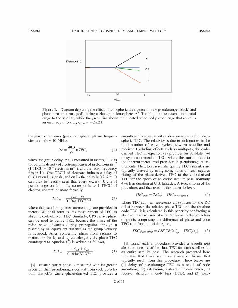
Figure 1. Diagram depicting the effect of ionospheric divergence on raw pseudorange (black) andphase measurements (red) during a change in ionosphere DI. The blue line represents the actualrange to the satellite, while the green line shows the updated smoothed pseudorange that containsan error equal to rangeerror = �2wDI.

RS6002 DYRUD ET AL.: IONOSPHERIC MEASUREMENT WITH GPS

2 of 11

RS6002

spheric divergence of pseudorange TEC resulting fromcode smoothing. We continue with a presentation of thesebiases, together with techniques for their mitigation.

3. Effects of Code Smoothing

[7] To mitigate inherent fluctuations in pseudorangedue to bandwidth limited precision, receiver noise, andmultipath, typical GPS receivers generally employ so-called phase smoothing or leveling of code. Phasesmoothing is essentially some combination of the noisycode pseudorange with the comparatively smoothlyvarying carrier phase. These smoothed pseudorangesare typically the only pseudorange output available to aGPS receiver user. As the following derivations demon-strate, this smoothness is achieved at the expense ofimposing bias on the code TEC estimate [Walter et al.,2004].[8] A standard definition for smoothed pseudorange

generally takes the following form, and is known as aHatch filter [Hatch, 1982],

Si ¼ wri þ ð1� wÞðSi�1 þ fi � fi�1Þ; ð6Þ

where Si is the smoothed pseudorange at time step i, r isthe raw pseudorange and ’ is the carrier phase, and w isa weight factor, between 0 and 1, that controls theeffective length of the smoothing filter in time.Generally, values of w are much less then 1 (0.01–0.001), which entails smoothing times ranging from 100to 1000 s. All the terms in equation (6) are written inunits of meters, so the carrier phase ’ = c/f’true, where cis the speed of light and f is the carrier frequency.[9] We can define raw pseudorange as having the

following components, still working in units of distancefor all quantities of interest,

ri ¼ ri þ Ii þMi þ biasr; ð7Þ

and similarly, the carrier phase can be defined as havingthe following components

fi ¼ ri � Ii þ biasf; ð8Þ

where ri represents the terms in common betweenpseudorange and phase, particularly range to the satellitein meters, troposphere delay, and receiver clock offset, Iirepresents the ionospheric correction in meters at timestep i, and Mi is the contribution of multipath, which hasbeen ignored in the phase measurements since itrepresents at least 1 order of magnitude smaller errorin phase than it does in pseudorange. As discussed inthe introduction, the ionospheric correction terms inequation (7) and equation (8) contain a negative sign forthe phase and a positive sign for the pseudorange. Thisproperty is known as ionospheric divergence and its

effect on navigation accuracy has been highlighted in anumber of recent articles [McGraw, 2006; Walter et al.,2004; Kim et al., 2006].[10] The following paragraphs demonstrate why this

phase smoothing may be desirable for navigation and aidin multipath mitigation, but it introduces two unwantedbiases in the calculation of absolute ionospheric TEC.These biases are:[11] 1. Phase smoothing of the code using a Hatch type

filter results in ionospheric divergence error. The error inpseudorange is approximately equal to �2DITsmooth, andthe error in code-derived ionospheric TEC is approxi-mately �DITsmooth.[12] 2. Such smoothing also causes the output of the

code calculated ionospheric correction to be delayedapproximately 0.3 Tsmooth, which introduces an errorapproximately equal to 0.3DI Tsmooth, where DI is theionospheric TEC rate of change represented in meters persecond and Tsmooth is the duration of the smoothing filter.[13] Smoothing induced bias arises when the iono-

spheric TEC changes from one time step to the next.This change in TEC can occur because of natural iono-spheric fluctuations and diurnal changes, or simplyduring each satellite pass through increasing and de-creasing elevation angles. Under such changes, even ifthe true satellite range does not change, equation (7) andequation (8) show that, the raw pseudorange will growlarger, and the phase will decrease by an equivalentamount. This divergence for one time step is depictedin Figure 1. If the ionospheric TEC continues to change,the smoothed pseudorange will continue to deviate fromthe actual range and will only recover once the iono-sphere stops changing for at least Tsmooth.

4. Ionospheric Divergence Effects on the

Calculation of Ionospheric Correction and

TEC

[14] Since receiver output pseudorange on L1 and L2

are used to derive the absolute ionospheric correction tothe pseudorange for navigation, and the absolute TEC forscientific measurement, ionospheric divergence errors inthe individual pseudoranges will bias the estimate ofionospheric correction (TEC). We continue with a deri-vation demonstrating this mathematically, and continuewith examples of ionospheric divergence bias in realGPS data.[15] The ionospheric correction in meters for L1 or the

equation for absolute code TEC (1 TEC unit = 16.3 cmof ionospheric correction on L1), is calculated as follows,

IonoSL1 ¼SL1i � SL2i

1� fL1=fL2� �2 ; ð9Þ


3 of 11

RS6002

and the phase TEC is calculated in a similar manner,

IonofL1 ¼�fL1i þ fL2i

1� fL1=fL2� �2 : ð10Þ

If we replace the definition of S from equation (6) intoequation (9), and assuming the weight factors for L1 andL2 are the same, and that DI from the previous time stepwas zero, we can examine the effect of ionosphericdivergence on ionospheric correction for 1 time step,

IonoSL1 ¼wrL1i þ ð1� wÞðSiL1�1 þ fL1i � fL1i�1Þ � wrL2i þ ð1� wÞðSL2i�1 þ fL2i � fL2i�1Þ

1� fL1=fL2� �2 : ð11Þ

[16] We continue by inserting the definitions for ’ andr from equations (7) and (8) and simplify by applyingthe definition, F = 1� fL1=fL2

� �2, and to avoid recursive

calculations we assume that the I of the previous timestep is zero such that SL1i�1 = SL2i�1, and that wL1 = wL2

yielding,

IonoSL1 ¼wðIL1 � IL2Þ þ ð1� wÞðDIL1 �DIL2Þ

F; ð12Þ

and since, DI = Ii and IL2 = IL1fL1=fL2� �2

, the equationreduces to

IonoSL1 ¼ �ð1� 2wÞIL1: ð13Þ

Now we may see that the difference between the trueionospheric correction on L1 and that estimated fromsmoothed pseudorange is opposite in direction andnearly (w 1) equal in magnitude. Therefore, iono-spheric divergence not only corrupts individual pseudor-anges, but this corruption is carried through to thecalculation of code TEC or ionospheric correction.

5. Mitigating Ionospheric Divergence With

a Divergence-Free Filter

[17] The use of a dual frequency GPS receiver allowsfor the novel mitigation of code smoothing inducedionospheric divergence. If we replace fi � fi�1 inequation (6) with a corrected ionospheric term, theeffects of ionospheric divergence are easily removed.

SDivFreei ¼ wri þ ð1� wÞðSi�1 þ fi � fi�1 þDIÞ;ð14Þ

where the change in ionosphere is obtained from the dualfrequency phase measurements,

DI ¼ �DfL1i þDfL2i

1� fL1=fL2� �2 : ð15Þ

It can thus be shown that such a smoothing algorithmwill not accumulate ionospheric divergence errors during

ionospheric changes. The following section demonstratesthese procedures on GPS data collected in Fairfax,Virginia.

6. Examples of Ionospheric Divergence and

Delay of TEC From GPS Data

[18] Figure 2 demonstrates an example of code TECand phase TEC from the celestial reference system GPS

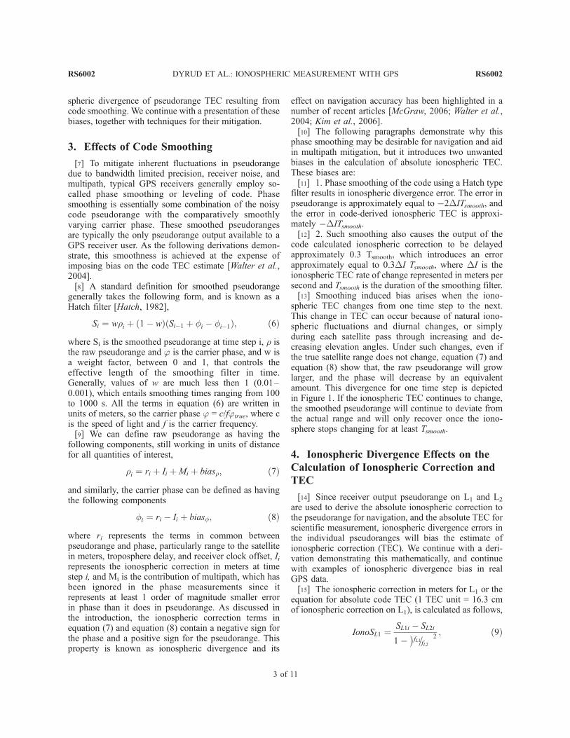
receiver for the first 10,000 s of observation of pseudo-random number 2 (PRN 2) on 30 November 2006. Thisdate, time, and PRN were chosen arbitrarily as a dem-onstration of typical data for a GPS receiver in thecontinental U.S. Figure 2 plots ionospheric TEC inmeters of L1 ionospheric correction. The plot displaysraw code TEC, with no smoothing, obtained from raw L1

and L2 pseudoranges in black. It should be noted herethat the raw code TEC displayed here has been smoothedby a centered 20 point boxcar average, so that 10 m pointto point fluctuations do not overwhelm Figure 2. Thiswas done only for plotting and not during the analysis.The phase TEC has been fit using the LSF methoddescribed above to the raw code TEC and is also shownin black. Two additional code TEC estimates are shown,which were calculated using two smoothing techniques.The first is the standard Hatch filter using a 500 ssmoothing time and is shown in blue. The second is a500 s ionospheric divergence free (Divfree) filter that isavailable using the CRS receiver and is shown in yellow.Both smoothed code TEC estimates are considerablysmoother then the raw TEC estimate that shows noiseand multipath fluctuations. Here the TEC is decreasingfrom 9 to 4 m over the course of 10,000 s as the satelliteincreases in elevation. The ionospheric change rate of 1 mper 2000 s induces between a 0.5–1 m ionosphericdivergence error over the 500 s smoothing time, as seenby comparing the yellow line to the blue. An additionalerror is induced by the delay effect of applying a trailingsmoothing such as the Hatch filter. This effect is shownto be between 0.5 and 1 m as well, as evidenced bycomparing the yellow code TEC to the black raw codeTEC. These data were collected raw at 50 Hz and thesmoothing was applied in post processing to demonstratethe effects of delay and ionospheric divergence with asfew other factors as possible. Comparisons using simul-taneously operating receivers in raw, Hatch-smoothed,and Divfree smoothing modes showed similar results asthese postprocessing results presented here. Additionalexamples of ionospheric divergence are shown in


4 of 11

RS6002

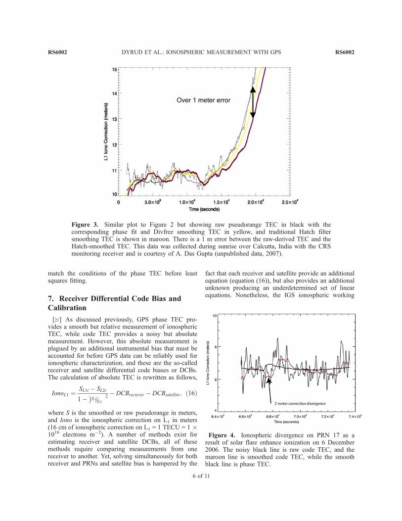
Figures 3 and 4. Figure 3 shows a rapid enhancement inionospheric TEC during sunrise in Calcutta, India, andFigure 4 shows a TEC enhancement during a solar flareon 6 December 2006. Our analysis of the solar flare datahas shown that all PRNs were subject to a, temporary, 2 mionospheric correction error during this period, whichcaused a persistent positioning error for nearly 30 min.[19] The fact that all code smoothing is conducted by a

trailing filter, imposes an unavoidable delay on thepseudorange output and particularly, code estimatedTEC. Figure 5 demonstrates the delay between smoothedpseudorange and raw pseudorange code TEC for theCRS receiver operating in raw mode and commonreceiver architecture used for TEC measurements theNovatel OEM 4 receiver. Our research has shown thatthe delay between true code TEC and smoothed codeTEC is approximately one-third Tsmooth. The observed30 s delay of the Novatel receiver indicates that itsmoothes using an approximately 100 s filter.[20] Figure 2 also demonstrates the effects that these

biases have on fitting the phase TEC to a biased codeTEC. Figure 2 showed that both the delay induced by

smoothing and the ionospheric divergence cause a com-bined 1.5 m bias in the TECFinal estimate. This error inabsolute TEC estimation of nearly 10 TECU, and issubstantial. Clearly a number of methods can be appliedto avoid these situations, such as using only high-elevation portions of satellite passes to conduct the leastsquares fit. However, doing so dramatically reduces thenumber of points available for the fit, diminishing theinherent accuracy of the fit. Further, such techniques areimpractical if quality real time or near real time TECestimates are required, since satellites always come intoview at low elevation angles, and demonstrate a decreas-ing ionosphere as that elevation increases. For the mostscientifically accurate postprocessed TEC estimation, wehave found that raw pseudoranges, with no smoothing,avoid both biases. If multipath is a significant concern,employing a ionospheric divergence free smoothing,such as the Divfree smoothing mode of the CRS Iono-spheric monitoring receiver to mitigate multipath, with-out inducing ionospheric divergence issues presents acompromise. Delay effects can then be mitigated byshifting code TEC ahead in time 0.3 Tsmooth to best

Figure 2. TEC estimation for PRN 2 from 30 November 2006. The plot displays rawpseudorange TEC (black) and smoothed using the ionospheric divergence free filter (yellow) andstandard Hatch smoothing filter (blue). Both smoothing times are 500 s. The corresponding phaseTEC fitted to each code TEC is shown by the smooth lines with corresponding color. Here theionospheric correction on L1 is decreasing from 9 to 4 m over the course of 10,000 s. Theionospheric change rate of 1 m per 2000 s induces at least a 0.5 m ionospheric divergence errorover the 500 s smooth. An additional error induced by the smoothing delay is shown to be nearly1 m as well. These data were collected raw at 50 Hz, and the smoothing was applied inpostprocessing to demonstrate the effects of delay and ionospheric divergence with as few otherfactors as possible.


5 of 11

RS6002

match the conditions of the phase TEC before leastsquares fitting.

7. Receiver Differential Code Bias and

Calibration

[21] As discussed previously, GPS phase TEC pro-vides a smooth but relative measurement of ionosphericTEC, while code TEC provides a noisy but absolutemeasurement. However, this absolute measurement isplagued by an additional instrumental bias that must beaccounted for before GPS data can be reliably used forionospheric characterization, and these are the so-calledreceiver and satellite differential code biases or DCBs.The calculation of absolute TEC is rewritten as follows,

IonoL1 ¼SL1i � SL2i

1� fL1=fL2� �2 � DCBreciever � DCBsatellite; ð16Þ

where S is the smoothed or raw pseudorange in meters,and Iono is the ionospheric correction on L1 in meters(16 cm of ionospheric correction on L1 = 1 TECU = 1 1016 electrons m�2). A number of methods exist forestimating receiver and satellite DCBs, all of thesemethods require comparing measurements from onereceiver to another. Yet, solving simultaneously for bothreceiver and PRNs and satellite bias is hampered by the

fact that each receiver and satellite provide an additionalequation (equation (16)), but also provides an additionalunknown producing an underdetermined set of linearequations. Nonetheless, the IGS ionospheric working

Figure 4. Ionospheric divergence on PRN 17 as aresult of solar flare enhance ionization on 6 December2006. The noisy black line is raw code TEC, and themaroon line is smoothed code TEC, while the smoothblack line is phase TEC.

Figure 3. Similar plot to Figure 2 but showing raw pseudorange TEC in black with thecorresponding phase fit and Divfree smoothing TEC in yellow, and traditional Hatch filtersmoothing TEC is shown in maroon. There is a 1 m error between the raw-derived TEC and theHatch-smoothed TEC. This data was collected during sunrise over Calcutta, India with the CRSmonitoring receiver and is courtesy of A. Das Gupta (unpublished data, 2007).


6 of 11

RS6002

group compiles a daily list of satellite DCBs and thecorresponding receiver DCB for about 100 worldwidereceivers using a Kalman Filter approach for combiningGPS data [Dow et al., 2005; Komjathy et al., 2005].These results are used to generate a publish GlobalIonosphere Maps (GIM) that have a quoted 2–9 TECUaccuracy and available for download at the NASA JetPropulsion Laboratory (JPL) website via ftp (http://igscb.jpl.nasa.gov/components/prods.html).[22] An additional common technique for estimating

receiver DCB is to assume that TEC is never negative, ornighttime vertical TEC values are near 1–3 TECU andtherefore the receiver DCB is the number necessary toeliminate negative TEC from all slant TEC observations.Such techniques yield approximate DCBs, and limit thetype of scientific study that can be conducted with theresulting data. However, instead of estimating receiverDCB, here we present a technique for measurement ofreceiver DCB to better than 1 cm, or less then 0.1 TECU.[23] In order to properly measure receiver DCB, the

CRS GPS receiver contains a patented internal calibratorthat measures absolute code delay and phase offset on L1

and L2 frequencies [Ganguly et al., 2007]. This isaccomplished by attaching a cable from a GPS signalgenerator with an output on the receiver box, to the

antenna input of the receiver. This allows for the directcharacterization of receiver DCB and any drift in phaseoffset that may occur between subsequent calibrations.Example results using this calibrator to derive accurateabsolute TEC are shown in Figure 6. Figure 6 comparesTEC from 7 December 2006 for a National GeodeticSurvey (NGS) Continuously Operating Reference Sta-tion GPS receiver LWX1 located in Sterling, Virginiaand the CRS GPS receiver located 15 km away inFairfax, Virginia. Slant TEC estimates are shown inred, and vertical TEC estimates are blue. Both receivers’TEC estimates have been adjusted for satellite DCBsusing the NASA JPL estimates available via ftp. TheCRS receiver DCB was adjusted using the internalcalibrator, and was found to be 13.3 TECU. TheLWX1 receiver DCB is unknown, but is clearly approx-imately �42 TECU. Figure 6 shows that without propercharacterization of the receiver DCB, the resulting TECestimates of NGS and IGS monitoring receivers do notprovide absolute TEC. Using the CRS internal calibratorwe have collected over 1 year of TEC data without evermeasuring negative TEC, a testament to the accuracy ofthe calibrator.[24] An additional, more detailed, test of instrumental

measurement of receiver DCB comes from comparing

Figure 5. Plot demonstrating the cross correlation between the CRS raw pseudorange TECestimation and the Novatel code pseudorange TEC estimation for simultaneous receiver operationusing the same antenna. The smoothing filter of the Novatel receiver clearly lags the rawpseudorange by approximately 30 s. This cross correlation was conducted over 20,000 s of datafrom PRN 1 on 29 November 2006.


7 of 11

RS6002

Figure 6. Twenty-four hours of slant and vertical TEC from 7 December 2006 for NationalGeodetic Survey Continuously Operating Reference Station GPS receiver LWX1 located inSterling, Virginia and the CRS GPS receiver in Fairfax, Virginia. These receivers are separated byapproximately 15 km. Slant TEC estimates are shown in red, and vertical TEC estimates are blue.Both receivers have been adjusted for satellite DCBs using the NASA Jet Propulsion Laboratoryestimates available via ftp. The CRS receiver DCB was measured using the internal calibrator andwas found to be 13.3 TECU. The LWX1 receiver DCB is unknown but is clearly approximately�42 TECU.


8 of 11

RS6002

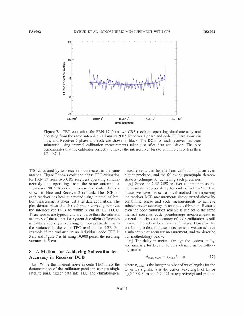
TEC calculated by two receivers connected to the sameantenna. Figure 7 shows code and phase TEC estimationfor PRN 17 from two CRS receivers operating simulta-neously and operating from the same antenna on1 January 2007. Receiver 1 phase and code TEC areshown in blue, and Receiver 2 in black. The DCB foreach receiver has been subtracted using internal calibra-tion measurements taken just after data acquisition. Theplot demonstrates that the calibrator correctly removesthe interreceiver DCB to within 5 cm or 1/2 TECU.These results are typical, and are worse than the inherentaccuracy of the calibration system due slight differencesin cabling and signal splitting, but are primarily due tothe variance in the code TEC used in the LSF. Forexample if the variance in an individual code TEC is5 m, and Figure 7 is fit using 10,000 points the resultingvariance is 5 cm.

8. A Method for Achieving Subcentimeter

Accuracy in Receiver DCB

[25] While the inherent noise in code TEC limits thedemonstration of the calibrator precision using a singlesatellite pass, higher data rate TEC and climatological

measurements can benefit from calibrations at an evenhigher precision, and the following paragraphs demon-strate a technique for achieving such precision.[26] Since the CRS GPS receiver calibrator measures

the absolute receiver delay for code offset and relativephase, we have devised a novel method for improvingthe receiver DCB measurements demonstrated above bycombining phase and code measurements to achievesubcentimeter accuracy in absolute calibration. Becauseeven the code calibration scheme is subject to the samethermal noise as code pseudorange measurements ingeneral, the absolute accuracy of code calibration is stilllimited in practice to a few centimeters. However, bycombining code and phase measurements we can achievea subcentimeter accuracy measurement, and we describeour methodology below.[27] The delay in meters, through the system on L1,

and similarly for L2, can be characterized in the follow-ing manner,

dcode=phase ¼ ncycleslþ f; ð17Þ

where ncycles is the integer number of wavelengths for theL1 or L2 signals, l is the center wavelength of L1 orL2(0.190294 m and 0.24421 m respectively) and ’ is the

Figure 7. TEC estimation for PRN 17 from two CRS receivers operating simultaneously andoperating from the same antenna on 1 January 2007. Receiver 1 phase and code TEC are shown inblue, and Receiver 2 phase and code are shown in black. The DCB for each receiver has beensubtracted using internal calibration measurements taken just after data acquisition. The plotdemonstrates that the calibrator correctly removes the interreceiver bias to within 5 cm or less then1/2 TECU.


9 of 11

RS6002

calibrator measured phase offset. ncycles is measuredusing the calibrator code delay in the following fashion,

ncyclesL1 ¼ ðdcodeL1 �modðcode offset;lL1ÞÞ=lL1; ð18Þ

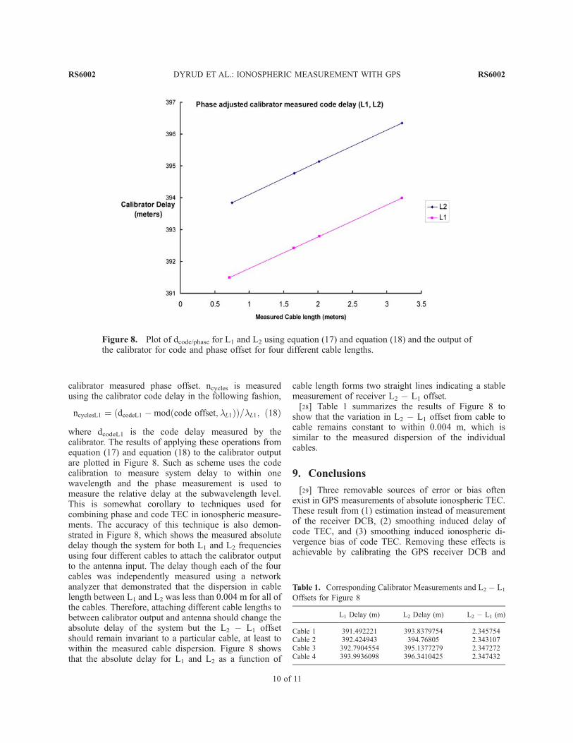
where dcodeL1 is the code delay measured by thecalibrator. The results of applying these operations fromequation (17) and equation (18) to the calibrator outputare plotted in Figure 8. Such as scheme uses the codecalibration to measure system delay to within onewavelength and the phase measurement is used tomeasure the relative delay at the subwavelength level.This is somewhat corollary to techniques used forcombining phase and code TEC in ionospheric measure-ments. The accuracy of this technique is also demon-strated in Figure 8, which shows the measured absolutedelay though the system for both L1 and L2 frequenciesusing four different cables to attach the calibrator outputto the antenna input. The delay though each of the fourcables was independently measured using a networkanalyzer that demonstrated that the dispersion in cablelength between L1 and L2 was less than 0.004 m for all ofthe cables. Therefore, attaching different cable lengths tobetween calibrator output and antenna should change theabsolute delay of the system but the L2 � L1 offsetshould remain invariant to a particular cable, at least towithin the measured cable dispersion. Figure 8 showsthat the absolute delay for L1 and L2 as a function of

cable length forms two straight lines indicating a stablemeasurement of receiver L2 � L1 offset.[28] Table 1 summarizes the results of Figure 8 to

show that the variation in L2 � L1 offset from cable tocable remains constant to within 0.004 m, which issimilar to the measured dispersion of the individualcables.

9. Conclusions

[29] Three removable sources of error or bias oftenexist in GPS measurements of absolute ionospheric TEC.These result from (1) estimation instead of measurementof the receiver DCB, (2) smoothing induced delay ofcode TEC, and (3) smoothing induced ionospheric di-vergence bias of code TEC. Removing these effects isachievable by calibrating the GPS receiver DCB and

Figure 8. Plot of dcode/phase for L1 and L2 using equation (17) and equation (18) and the output ofthe calibrator for code and phase offset for four different cable lengths.

Table 1. Corresponding Calibrator Measurements and L2 � L1

Offsets for Figure 8

L1 Delay (m) L2 Delay (m) L2 � L1 (m)

Cable 1 391.492221 393.8379754 2.345754Cable 2 392.424943 394.76805 2.343107Cable 3 392.7904554 395.1377279 2.347272Cable 4 393.9936098 396.3410425 2.347432


10 of 11

RS6002

operating a GPS receiver with no code smoothing orDivfree smoothing with delay adjustment to code TEC.Improved accuracy in absolute ionospheric TEC meas-urements will enhance the accuracy of global ionosphericreconstructions, and reduce error in conversion fromslant to vertical TEC, see Ganguly and Brown [2001].

[30] Acknowledgments. The authors would like to thankJeanette Johnson for her help in preparation of this paper.

References

Brown, A., and S. Ganguly (2001), Ionospheric tomography:

Issues, sensitivities, and uniqueness, Radio Sci., 36(4), 745–

755, doi:10.1029/1999RS002414.

Ciraolo, L., F. Azpilicueta, C. Brunini, A. Meza, and S. M.

Radicella (2007), Calibration errors on experimental slant

total electron content (TEC) determined with GPS, J. Geod.,

81(2), 111–120, doi:10.1007/s00190-006-0093-1.

Dow, J. M., R. E. Neilan, and G. Gendt (2005), The Interna-

tional GPS Service (IGS): Celebrating the 10th anniversary

and looking to the next decade, Adv. Space Res., 36(3),

320–326, doi:10.1016/j.asr.2005.05.125.

Dyrud, L., N. Bhatia, S. Ganguly, and A. Jovancevic (2006),

Performance analysis of software based GPS receiver using

a generic ionosphere scintillation model, paper presented at

19th International Technical Meeting, Satell. Div. of the Inst.

of Navig., Fort Worth, Tex.

Ganguly, S., and A. Brown (2001), Real-time characterization

of the ionosphere using diverse data and models, Radio Sci.,

36(5), 1181–1197, doi:10.1029/1999RS002412.

Ganguly, S., A. Jovancevic, and A. Brown (2007), Ionospheric

receiver with calibrator, Patent 722131 B2, U. S. Patent and

Trademark Off., Washington, D. C.

Hatch, R. R. (1982), The synergism of GPS code and carrier

measurements, J. Geod., 57(1–4), 207–208.

Kim, E., T. Walter, and J. D. Powell (2006), Optimizing WAAS

accuracy/stability for a single frequency receiver, paper pre-

sented at 19th International Technical Meeting, Satell. Div.

of the Inst. of Navig., Fort Worth, Tex.

Komjathy, A., L. Sparks, B. Wilson, and A. J. Mannucci (2005),

Automated daily processing of more than 1000 ground-based

GPS receivers to study intense ionospheric storms, Radio

Sci., 40, RS6006, doi:10.1029/2005RS003279.

McGraw, G. (2006), GNSS solutions, Inside GNSS, 1(5),

16–19.

Walter, T., J. Blanch, and J. Rife (2004), Treatment of biased

error distributions in SBAS, paper presented at Int. Symp. on

GPS/GNSS, Univ. of N. S. W., Sydney, Aust.

��A. Brown, L. Dyrud, S. Ganguly, A. Jovancevic, and

D. Wilson, Center for Remote Sensing, Inc., 3702 Pender

Drive, Suite 170, Fairfax, VA 22030, USA. (www.cfrsi.com)


11 of 11

RS6002

Ionospheric measurement with GPS: Receiver techniques and methods

Documents

Transcript of Ionospheric measurement with GPS: Receiver techniques and methods