1 1966

^ecknical rlote 92o. 337

ADVANCES IN IONOSPHERIC MAPPING BY

NUMERICAL METHODS

WILLIAM B. JONES, RONALD P. GRAHAM AND MARGO LEFTIN

U. S. DEPARTMENT OF COMMERCENATIONAL BUREAU OF STANDARDS

THE NATIONAL BUREAU OF STANDARDS

The National Bureau of Standards is a principal focal point in the Federal Government for assuring

maximum application of the physical and engineering sciences to the advancement of technology in

industry and commerce. Its responsibilities include development and maintenance of the national stand-

ards of measurement, and the provisions of means for making measurements consistent with those

standards; determination of physical constants and properties of materials; development of methodsfor testing materials, mechanisms, and structures, and making such tests as may be necessary, particu-

larly for government agencies; cooperation in the establishment of standard practices for incorpora-

tion in codes and specifications; advisory service to government agencies on scientific and technical

problems; invention and development of devices to serve special needs of the Government; assistance

to industry, business, and consumers in the development and acceptance of commercial standards andsimplified trade practice recommendations; administration of programs in cooperation with United

States business groups and standards organizations for the development of international standards of

practice; and maintenance of a clearinghouse for the collection and dissemination of scientific, tech-

nical, and engineering information. The scope of the Bureau's activities is suggested in the following

listing of its four Institutes and their organizational units.

Institute for Basic Standards. Electricity. Metrology. Heat. Radiation Physics. Mechanics. Ap-plied Mathematics. Atomic Physics. Physical Chemistry. Laboratory Astrophysics.* Radio Stand-

ards Laboratory: Radio Standards Physics; Radio Standards Engineering.** Office of Standard Ref-

erence Data.

Institute for Materials Research. Analytical Chemistry. Polymers. Metallurgy. Inorganic Mate-

rials. Reactor Radiations. Cryogenics.** Office of Standard Reference Materials.

Central Radio Propagation Laboratory.** Ionosphere Research and Propagation. Troposphereand Space Telecommunications. Radio Systems. Upper Atmosphere and Space Physics.

Institute for Applied Technology. Textiles and Apparel Technology Center. Building Research.

Industrial Equipment. Information Technology. Performance Test Development. Instrumentation.

Transport Systems. Office of Technical Services. Office of Weights and Measures. Office of Engineer-

ing Standards. Office of Industrial Services.

* NBS Group, Joint Institute for Laboratory Astrophysics at the University of Colorado.** Located at Boulder, Colorado.

NATIONAL BUREAU OF STANDARDS

technical ^ote 337ISSUED May 12, 1966

ADVANCES IN IONOSPHERIC MAPPINGBY NUMERICAL METHODS

William B. Jones, Ronald P. Graham and Margo Leftin

Institute for Telecommunication Sciences and Aeronomy :

Environmental Science Services Administration

Boulder, Colorado

NBS Technical Notes are designed to supplement the Bu-reau's regular publications program. They provide a

means for making available scientific data that are of

transient or limited interest. Technical Notes may belisted or referred to in the open literature.

"" Formerly the Central Radio Propagation Laboratory of the National Bureau of Standards.

CRPL was transferred to ESSA in October 1965, but will temporarily use NBS publicationseries pending inauguration of their ESSA counterparts.

For sale by the Superintendent of Documents, U. S. Government Printing Office

Washington, D.C. 20402

P rice: 4 5 <t

CONTENTS

Page

1. Introduction 1

2. Screen Analysis k

3. Second Analysis 16

3-1 Geographic Variation 17

3.2 Diurnal Variation 22

h. Comparison of Different Analyses „ . 28

5. Application of Numerical Maps 31

5.1 Simplified Expression of Q(\,9,T) 31

5.2 Calculation of Magnetic Dip I 36

5.3 Fortran Program 38

6. References kk

Appendix A Fourier Coefficients for foF2 Monthly Median . . Vf

Appendix B Contour Maps of Orthonormal Functions 57

Appendix C Diurnal Variation of Orthonormal Coefficients d, 63

Appendix D SAMPLE Program Listing 68

111

ADVANCES IN IONOSPHERIC MAPPING BY NUMERICAL METHODS

by

William B. Jones, Ronald P. Graham and Margo Leftin

Paper describes recent progress made at ITSA ( formerlyCRPL) to improve numerical methods for mapping and predictingionospheric characteristics used in telecommunication. Twomajor problems are considered: (l) tendency of maps to smoothout physical properties of the ionosphere, particularly atlow latitudes and (2) ambiguous values at geographic polesand resulting distortions in immediate surroundings. Thesecond problem is overcome by means of a universal timeanalysis. Significant improvement is made in the firstproblem by the use of a modified magnetic dip coordinate. Ageneral description is given of the new procedures for forming

numerical maps, including a number of illustrations. Alsoincluded are a discussion of the use of numerical maps in therevised form and a Fortran Program for evaluating numericalmaps of ionospheric characteristics and for calculating the

MQF(ZER0)F2 and MUF( IjOOO )F2

.

1. Introduction

In recent years the Institute for Telecommunication Sciences and

Aeronomy (formerly the Central Radio Propagation Laboratory) has been

engaged in the development of numerical methods and computer programs

for mapping and predicting characteristics of the ionosphere used in

telecommunication. Work along these lines was initiated prior to the

International Geophysical Year, with the first descriptive publication

appearing in the Telecommunication Journal [Jones and Gallet, i960]

.

Since that time numerous technical papers have been written to describe

the further advances in: (a) methods for data analysis and representat-

ion of ionospheric characteristics [Jones, 1962; Jones and Gallet,

1962a, 1965a, 1965b], (b) methods for applying numerical maps of

ionospheric characteristics [Jones and Gallet, 1962b], and

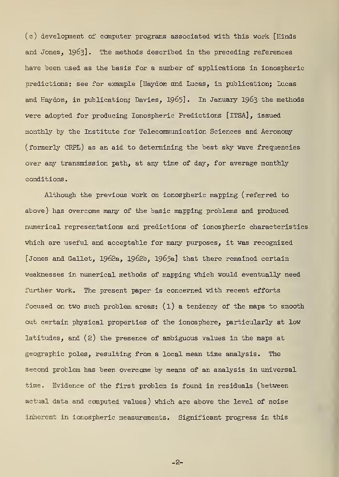
( c ) development of computer programs associated with this work [Hinds

and Jones, 1963] • ^e methods described in the preceding references

have been used as the basis for a number of applications in ionospheric

predictions: see for example [Haydon and Lucas, in publication; Lucas

and Haydon, in publication; Davies, 1965] • ^n January I963 the methods

were adopted for producing Ionospheric Predictions [ITSA], issued

monthly by the Institute for Telecommunication Sciences and Aeronomy

(formerly CRPL) as an aid to determining the best sky wave frequencies

over any transmission path, at any time of day, for average monthly

conditions.

Although the previous work on ionospheric mapping ( referred to

above) has overcome many of the basic mapping problems and produced

numerical representations and predictions of ionospheric characteristics

which are useful and acceptable for many purposes, it was recognized

[Jones and Gallet, 1962a, 1962b, 1965a] that there remained certain

weaknesses in numerical methods of mapping which would eventually need

further work. The present paper is concerned with recent efforts

focused on two such problem areas: (l) a tendency of the maps to smooth

out certain physical properties of the ionosphere, particularly at low

latitudes, and (2) the presence of ambiguous values in the maps at

geographic poles, resulting from a local mean time analysis. The

second problem has been overcome by means of an analysis in universal

time. Evidence of the first problem is found in residuals (between

actual data and computed values) which are above the level of noise

inherent in ionospheric measurements. Significant progress in this

-2-

area has "been achieved by taking into account more explicitly the

relationship between ionospheric characteristics and the magnetic field.

Previous studies have indicated the dependence of the ionosphere on the

magnetic field, particularly at low latitudes.

The revised methods and programs described in this paper have been

used to produce a provisional Atlas of Ionospheric Characteristics for

consideration at the 12th Plenary Assembly of CCIR to be held at Oslo,

Norway, June 1966. For this Atlas, two characteristics have been

analyzed: monthly median of the F2 layer critical frequency (foF2) for

all months of the five year period extending from 195^ through 1958, and

monthly median of M(3000)F2 for all months of 195^ and I958. The revised

method will also soon be used as the basis for ITSA Ionospheric Predict-

ions.

The intention of the present paper is to give a general descript-

ion of the new procedures for ionospheric mapping, with emphasis on

illustrating various main steps by means of graphs, maps, and tables.

Also included are: (l) a comparison of results from two different types

of analyses, (2) a careful discussion of how to apply numerical maps of

ionospheric characteristics in their present (revised) form and (3) a

FORTRAN program for evaluating numerical maps of ionospheric character-

istics and for calculating MUF(ZER0)F2 and MUF(^000)F2 (Appendix D).

By way of illustration we have used only the characteristic, foF2

median, since it is the most interesting and important for telecommunic-

ation.

[GHQ United States Army, 19^6; Appleton, 191*6; Bailey, 191*8]

-3-

2. Screen Analysis

As in the previous paper by Jones and Gallet [1965a] the numerical

mapping procedures described here involve two principal analyses of the

data, both performed in one pass on the computer. First, a so-called

"screen analysis" is made of available A- and B-data to produce approx-

imate values of the ionospheric characteristic (called "C-data") at

carefully chosen locations ("screen points") in large regions, such as

oceans, where no stations are available. These regions will be called

the critical areas. The C-data are then combined with the original A-

and B-data in forming a second (and final) analysis. The purpose of

C-data, discussed at length in the preceding reference, is to control

instabilities in the maps, which tend to develop in the critical areas.

The screen analysis is started by Fourier analyzing the monthly

medians of foF2 for each station for the 2k hours of the day. Thus the

diurnal variation at each place is decomposed into eleven harmonics

a . cos jt + b . sin jt = c . cos( jt - ^ . ), 1 = j = 11, ( l)J J J J

2and a constant term a which is the arithmetic mean of the 2^+ medians .

o

Here t denotes the local mean hour angle ( -l80° ^ t =? l80° , t = 0° at

noon IMT). Each harmonic is defined by an amplitude c. and phase i|r.,

<J

The terms A- and B-data are defined in the above references. In short,

A-data refer to measurements at stations taken during the actual monthin question. B-data refer to values of the characteristic obtained frominterpolation or extrapolation in time at a station which did not reportdata for the specific month in question but was active for a period of

time before or after. B-data are used to fill gaps where A-data are notavailable (Fig. l).

2There is also an additional term a cos 12t which is omitted since itdoes not form a complete harmonic and is produced mainly by noise.

-4-

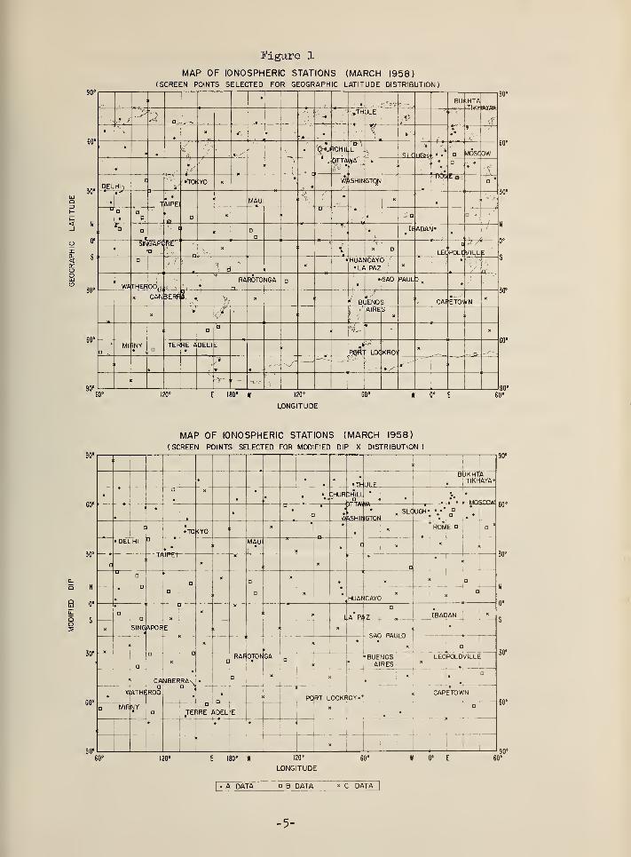
Figure 1

MAP OF IONOSPHERIC STATIONS (MARCH 1958)(SCREEN POINTS SELECTED FOR GEOGRAPHIC LATITUDE DISTRIBUTION)

< N -

2f S

i

•. % .. .,,, . BUICHTA

90

>'J:>

i2... a . •

""Hi''

-,,'THULE.$»

'•' r *

tfc

• "<

t

'i'. s r#~ .• 'i v";

.*•»

' •

.~/(l

«/-''"

•

•

'Chu RCHIL 1 .

h si rJJSii;.* • a MOSCOW

60

:

;'s(il IA

fa'?*, *

> :

'

\- #•

\

DEL HIt

c

r•Tor ;yo X w) kSHIN GTO^J

• RON K ,D i

a'

30

•»TAIPEI MAU "\V 1

•/•«

.:

P a «

• ,

* id - '

N

s

^1

t

'••'{

j caa

'%: '• IE ADAH*

Sll> GAPtjift£; v x i :

* *'

i'i

LECPOLCVILL I

..''. i'

:

«HUAr•u

JCAYI

PAZ> i

X /

•

vj

WATHEF°°rii

aRAROTO JGA D

.

* SAO PAULD,.

'

30'

« CANBERRV->

« 3 : LIe'no:

CAf ETOWN«

«V // ] :

1 )f

'

AIRE 3

:

J a i c k. -«

60

D, t

Ml WYD

TEF RE * DELIt

ROFh' LOCKRO^tX

T

;j,r— ^''

,

—

"Vir

%E 180" W 120'

LONGITUDE

W 1E

MAP OF IONOSPHERIC STATIONS (MARCH 1958)

(SCREEN POINTS SELECTED FOR MODIFIED DIP X DISTRIBUTION)w

60°

3

• \ •

•TH III F

BIJKHTOTIKHAYA-

*

-. •"

a X

•

•

• • v :hur :hill•

. wnprnuu

•C t w«Hliifimiv

' tSLC UGH' • .* D

O

•DEI

d•TOKYO

XX *ROME a a

-HI D3 c

MAU) [

•c *

*

N

0°

S

30°

3

60"

3

90"

D3 t

"-

X

)

xa

•

0.

ua

— o- -

—

D

D o

a

X.

ICAYC

X X D

nX •

HUAfI

>

1

UJ

»

o

SING

a

APOfi

D

X

E

NBEF

a

•

RAvo \

t

X

>

3 :

J. AJ?<kZ_D

IBAC AN

O5 >

3 :

•

X a

—i

RAF^OTONGA '

Q

.i

3 ;

»BUEANOSRES

LEOI

*

POLDVILLE

1 CAo

ATHEROO

)

PClRT L

!

[

~i

'

ockRoy.'

«! .

•

E

(x CAPETOWN

D»

a MIR NYD

n*RE ADEL

i .•

:

•" •

i

• i

120° E 180" W 120*

LONGITUDE

W 0* E

• A DATA a B DATA C DATA

-5-

equivalently, by cosine and sine coefficients a. and b ., respectively.

Harmonics above the eighth order are dropped since they are produced more

by noise than by real physical variation [ Jones, 1962; Jones and

Gallet, 1962a and 1965b ].

Basically, the purpose of the screen analysis is to reduce the major

part of the two-dimensional geographic variation of each Fourier

coefficient a. and b. (j s8) to that of a single variable x, "which inj J

general may be a function of both geographic latitude \ and longitude 0.

Since there will be no large gaps in the distribution of stations in the

one dimension of x, an approximate representation of the ionospheric

characteristic can be obtained as a function of x "without the danger of

instability. Accordingly, the Fourier coefficients a. and b. areJ d

represented geographically (to a first approximation) by a series of the

formK

Ik=0

\ Gfc(x), (2)

"where the functions G, (x) may be powers of x or sin x, or some other

functions. The coefficients D are determined by the method of least

squares and the cutoff K is made (by the computer) using a Student's t

test [Jones and Gallet, 1962a] . Thus the approximate representation of

the ionospheric characteristic has the form

8

T(x, t) = aQ(x) + \ a (x) cos jt + b^x) sin jtl , (3)

j=l

where a.(x) and b.(x) represent the Fourier coefficients as functions ofJ J

x in the form ( 2 )

.

-6-

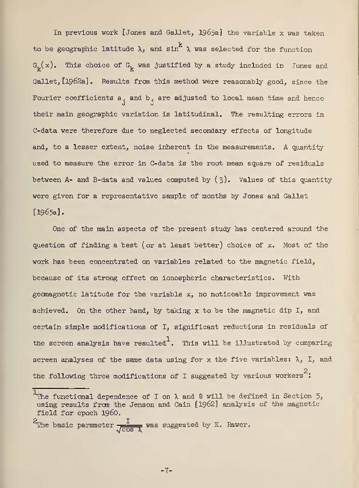
In previous work [Jones and Gallet, 1965a] the variable x was taken

to be geographic latitude X, and sin X was selected for the function

G, (x). This choice of G, was justified by a study included in Jones and

Gallet, [1962a] . Results from this method were reasonably good, since the

Fourier coefficients a . and b . are adjusted to local mean time and henced J

their main geographic variation is latitudinal. The resulting errors in

C-data were therefore due to neglected secondary effects of longitude

and, to a lesser extent, noise inherent in the measurements. A quantity

used to measure the error in C-data is the root mean square of residuals

between A- and B-data and values computed by (3)« Values of this quantity

were given for a representative sample of months by Jones and Gallet

[1965a]

.

One of the main aspects of the present study has centered around the

question of finding a best (or at least better) choice of x. Most of the

work has been concentrated on variables related to the magnetic field,

because of its strong effect on ionospheric characteristics. With

geomagnetic latitude for the variable x, no noticeable improvement was

achieved. On the other hand, by taking x to be the magnetic dip I, and

certain simple modifications of I, significant reductions in residuals of

the screen analysis have resulted . This will be illustrated by comparing

screen analyses of the same data using for x the five variables: X, I, and

2the following three modifications of I suggested by various workers :

1The functional dependence of I on X and 9 will be defined in Section 5,

using results from the Jenson and Cain [1962] analysis of the magnetic

field for epoch i960.2 IThe basic parameter r "was suggested by K. Rawer.

^cos X

-7-

Tan-1

vcos X

w

Tan-1 tan I

>Tc

(5)cos X

x = Tan-1 tan I

j/cos (x - 5)_

(6)

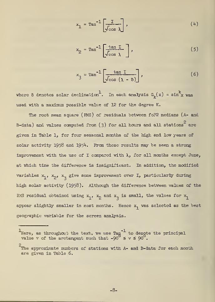
where 5 denotes solar declination . In each analysis G, (x) = sin x was

used with a maximum possible value of 12 for the degree K.

The root mean square (EMS) of residuals between foF2 medians (A- and

B-data) and values computed from (3) for all hours and all stations are

given in Table 1, for four seasonal months of the high and low years of

solar activity 1958 and 19 5^ • From these results may be seen a strong

improvement with the use of I compared with X, for all months except June,

at which time the difference is insignificant. In addition, the modified

variables x , x„, x give some improvement over I, particularly during

high solar activity (1958). Although the difference between values of the

RMS residual obtained using x , xp

and x is small, the values for x_

appear slightly smaller in most months. Hence x.. was selected as the best

geographic variable for the screen analysis.

iiere, as throughout the text, we use Tan to denote the principalvalue v of the arctangent such that -90 ^ v ^ 90 .

2The approximate numbers of stations with A- and B-data for each monthare given in Table 6.

-8-

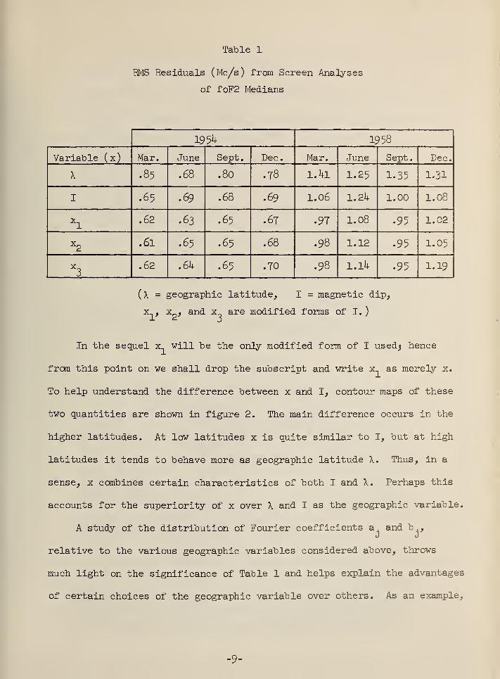
Table 1

RMS Residuals (Mc/s) from Screen Analyses

of foF2 Medians

1954 1958

Variable (x) Mar. June Sept. Dec. Mar. June Sept. Dec.

X •85 .68 .80 .78 1.41 1.25 1.35 1^31

I .65 .69 .68 .69 1.06 1.24 1.00 1.08

Xl

.62 .63 .65 .67 • 97 1.08 • 95 1.02

X2

.61 .65 .65 .68 .98 1.12 • 95 1.05

X3

.62 .64 .65 .70 • 98 1.14 • 95 1.19

( X - geographic latitude, I - magnetic dip,

x , x , and x are modified forms of I.

)

In the sequel x will be the only modified form of I usedj hence

from this point on ve shall drop the subscript and write xn

as merely x.

To help understand the difference between x and I, contour maps of these

two quantities are shown in figure 2. The main difference occurs in the

higher latitudes. At low latitudes x is quite similar to I, but at high

latitudes it tends to behave more as geographic latitude X. Thus, in a

sense, x combines certain characteristics of both I and X. Perhaps this

accounts for the superiority of x over X and I as the geographic variable.

A study of the distribution of Fourier coefficients a. and b ,J J

relative to the various geographic variables considered above, throws

much light on the significance of Table 1 and helps explain the advantages

of certain choices of the geographic variable over others. As an example,

-9-

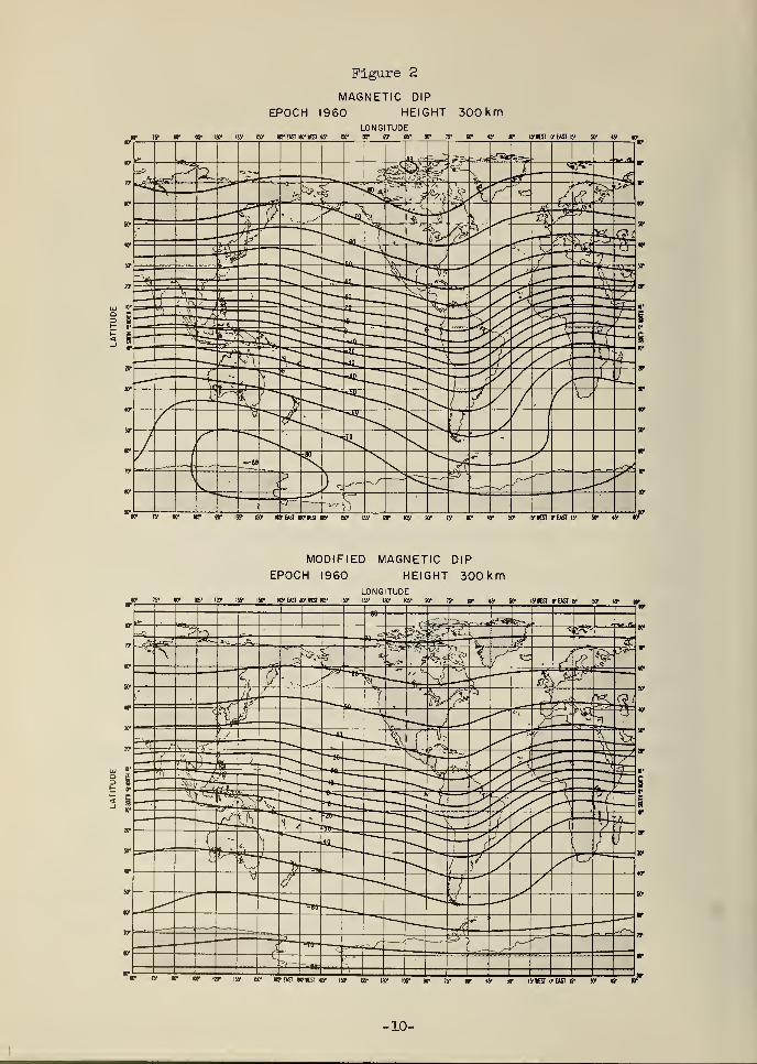
Figure 2

MAGNETIC DIP

EPOCH I960 HEIGHT 300 kmLONGITUDE

kw is- ijy w «S"Ejsi Kritstus1 ar ii> ar « w is1 <y air is-kst cr east b- w w tr

M" 73' »• W Of \5t BO" WEASI KTIESr

MODIFIED MAGNETIC DIP

EPOCH I960 HEIGHT 300 km

«• w ij? bc trust wkst us- iw !»• w kb- »• »• w «• » ii-iesi o-easi iv »• w

10-

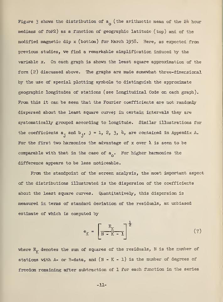
Figure 3 shows the distribution of a ( the arithmetic mean of the 2k hour

medians of foF2) as a function of geographic latitude (top) and of the

modified magnetic dip x (bottom) for March 1958. Here, as expected from

previous studies, we find a remarkable simplification induced by the

variable x. On each graph is shown the least square approximation of the

form (2) discussed above. The graphs are made somewhat three-dimensional

by the use of special plotting symbols to distinguish the approximate

geographic longitudes of stations (see Longitudinal Code on each graph).

From this it can be seen that the Fourier coefficients are not randomly

dispersed about the least square curve; in certain intervals they are

systematically grouped according to longitude. Similar illustrations for

the coefficients a. and b ., j =1, 2, 3, k, are contained in Appendix A.

For the first two harmonics the advantage of x over X is seen to be

comparable with that in the case of a . For higher harmonics the

difference appears to be less noticeable.

From the standpoint of the screen analysis, the most important aspect

of the distributions illustrated is the dispersion of the coefficients

about the least square curves. Quantitatively, this dispersion is

measured in terms of standard deviation of the residuals, an unbiased

estimate of which is computed by

(T)

where E^ denotes the sum of squares of the residuals, N is the number of

stations with A- or B-data, and (N - K - l) is the number of degrees of

freedom remaining after subtraction of 1 for each function in the series

o — rek

l2

eK

"N - K - 1

-11-

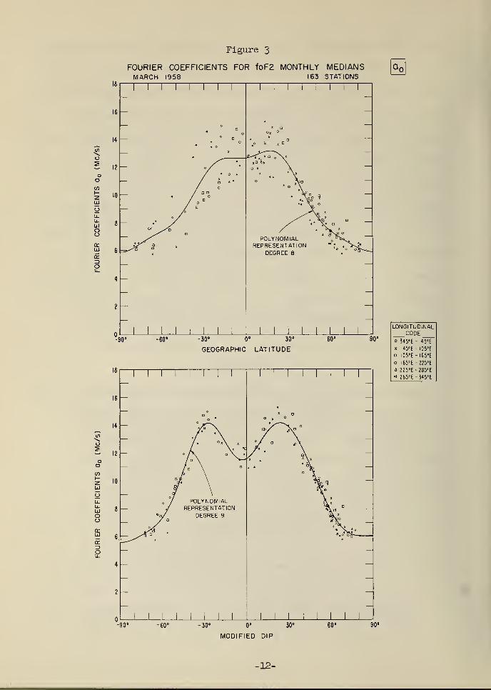
Figure 3

FOURIER COEFFICIENTS FOR foF2 MONTHLY MEDIANSMARCH 1958 163 STATIONS

16—

4—

2—

-90°

-90°

a - d

POLYNOMIALREPRESENTATION

DEGREE 8

-60° -30° 0° 30° 60°

GEOGRAPHIC LATITUDE

-60° -30" 0° 30°

MODIFIED DIP

60°

90°

id1 1 1 1 1 1 1 1 1 1 1 1

1 1 1

16

Oo x

DO

14— Vr\ \*>/ A?

—(/) «/ \o 1 * °x\ x °y ° i>\? / \ k

*:

11!— O /X o \ K o\

—o / ° \ —

'

* ^ Ao — /d \ ° * *d\ —

in o

h-z 10

— "a? \ ^k SI

—LiJ f \ *&*o —

o/—

U_ / POLYNOMIAL A *

u_» / REPRESENTATION V ° —

o »o/ DEGREE 9 & <

o / a «V —rr */^ *

* ^s^,*«

UJ6

/"a a

a:->

£4

2

n 11 1 1 1 1 1 1

1 11

1

1 1 1

90°

LONGITUDINALCODE

o 345°E • 45'E

« 45'E I05'E

a 1 05°E - I65"E

o I65'E -225'E

fl 225'E •285'E

« 285'E -345°E

12-

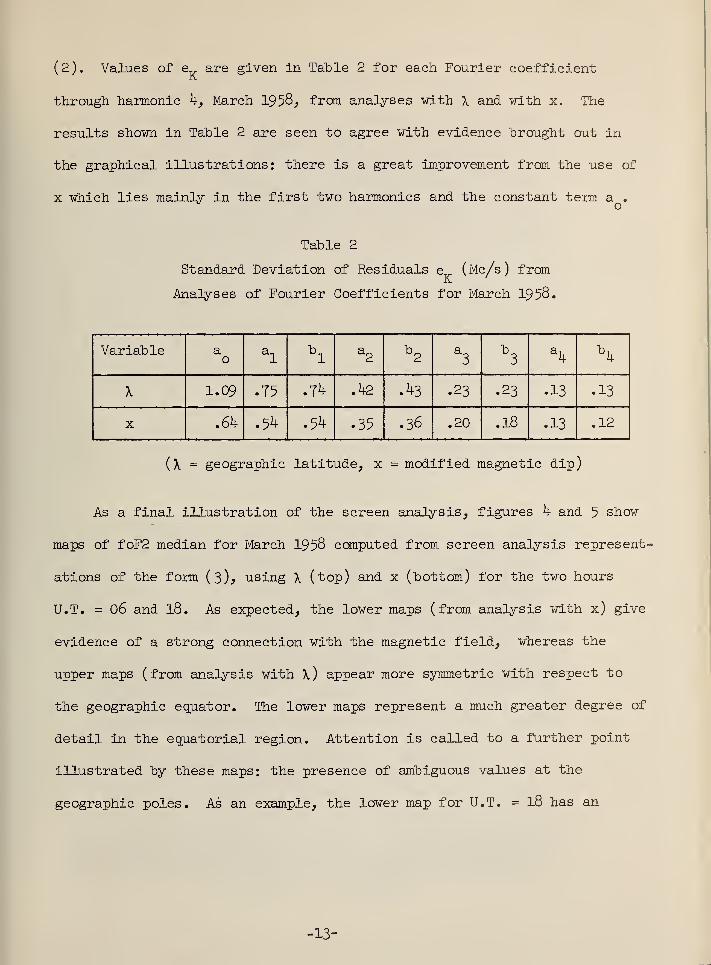
(2). Values of e are given in Table 2 for each Fourier coefficient

through harmonic 4, March 1958, from analyses with \ and with x. The

results shown in Table 2 are seen to agree with evidence brought out in

the graphical illustrations: there is a great improvement from the use of

x which lies mainly in the first two harmonics and the constant term a .^ o

Table 2

Standard Deviation of Residuals e (Mc/s) from

Analyses of Fourier Coefficients for March 1958.

Variable ao

al

bl

a2 \ a

3b3

a4

b4

X 1.09 .75 .74 .42 M .23 .23 .13 .13

X .64 • 54 .& • 35 .36 .20 .18 .13 .12

(X = geographic latitude, x = modified magnetic dip)

As a final illustration of the screen analysis, figures 4 and 5 show

maps of foF2 median for March 1958 computed from screen analysis represent-

ations of the form (3), using \ (top) and x (bottom) for the two hours

U.T. = 06 and 18. As expected, the lower maps (from analysis with x) give

evidence of a strong connection with the magnetic field, whereas the

upper maps (from analysis with \) appear more symmetric with respect to

the geographic equator. The lower maps represent a much greater degree of

detail in the equatorial region. Attention is called to a further point

illustrated by these maps: the presence of ambiguous values at the

geographic poles. As an example, the lower map for U.T. = 18 has an

-13-

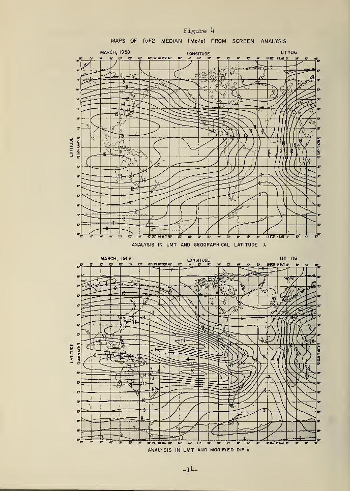
Figure h

MAPS OF foF2 MEDIAN (Mc/s) FROM SCREEN ANALYSIS

MARCH, 1958 LONGITUDE UT =06so- is- w ids' w ny isc CEASTm-tsr^' «r ay w «• »• ts

1 jc ty iir lynsr o-east s* »• 4y to*

75' 9C 105" US' ISO* IS? EAST WIEST «y ISO1

US' 120" 105' »• 75' 6T 45' JC IS- WEST 0" EAST IS* XT «f «P

ANALYSIS IN LMT AND GEOGRAPHICAL LATITUDE X

MARCH, 1958 LONGITUDE UT=06jr Ty w ipy ize- 'is* or ig eastw ibt ny B'gififffiyi'ii' 30* lyitsi ceast ry ate w

»• ts- nr m » ijj> w «t easi ncriea «s- w v i!ir »' v is' v c v lyRSi ceast ly

ANALYSIS IN LMT AND MODIFIED DIP x

-lk-

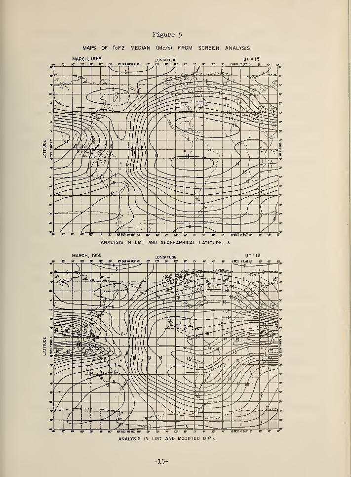
Figure 5

MAPS OF foF2 MEDIAN (Mc/s) FROM SCREEN ANALYSIS

MARCH, 1958 LONGITUDE UT = 18

n> 75' UT «»• ar u? mr c-EASHo-isnty isc i» w us- w ry or <y iy gust o-asi b- jp « «•

80- 15' W KB- BT UP ISO- IW EAST WIEST 165* ISO- US- HP 105' 90' 15' SO* «• JO- IS1(EST 0- EAST IS- XT «•

ANALYSIS IN LMT AND GEOGRAPHICAL LATITUDE X

UT=I8

D1 IT V V * V «BS W«S W" OT US' 1ST W 10" IS1 • «5* »" ITKSI if EAST S- » «T

ANALYSIS IN LMT AND MODIFIED DIP x

-15-

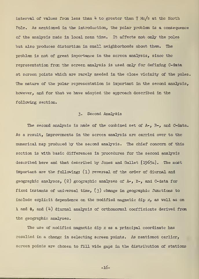
interval of values from less than k to greater than 7 Mc/s at the North

Pole. As mentioned in the introduction, the polar problem is a consequence

of the analysis made in local mean time. It affects not only the poles

but also produces distortion in small neighborhoods about them. The

problem is not of great importance in the screen analysis, since the

representation from the screen analysis is used only for defining C-data

at screen points which are rarely needed in the close vicinity of the poles,

The nature of the polar representation is important in the second analysis,

however, and for that we have adopted the approach described in the

following section.

3. Second Analysis

The second analysis is made of the combined set of A-, B-, and C-data.

As a result, improvements in the screen analysis are carried over to the

numerical map produced by the second analysis. The chief concern of this

section is with basic differences in procedures for the second analysis

described here and that described by Jones and Gallet [1965a]. The most

important are the following: (l) reversal of the order of diurnal and

geographic analyses, (2) geographic analyses of A-, B-, and C-data for

fixed instants of universal time, '( 3 ) change in geographic functions to

include explicit dependence on the modified magnetic dip x, as well as on

X and 9, and (k) diurnal analysis of orthonormal coefficients derived from

the geographic analyses.

The use of modified magnetic dip x as a principal coordinate has

resulted in a change in selecting screen points. As mentioned earlier,

screen points are chosen to fill wide gaps in the distribution of stations

-16-

where instabilities might develop. The use of x and 9 as principal

coordinates ( instead of X and 8 ) has the effect of transforming the

station distribution and hence of changing the shape and size of the gaps.

Thus it is necessary to select different screen points from those used in

previous analyses. As an illustration, the station distribution for

March 1958 is shown in figure l(a) in (\, 9) coordinates and figure l(b)

in (x, 9) coordinates. The sets of screen points selected for the former

distribution and for the transformed distributions are shown in the

respective maps by the use of special plotting symbols (see captions). As

in the previous case, the set of screen points changes very little from

month to month.

3.1 Geographic Variation

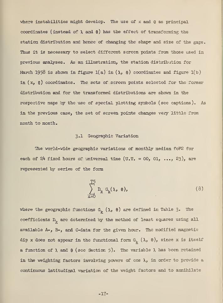
The world-wide geographic variations of monthly median foF2 for

each of 2k fixed hours of universal time (U.T. = 00, 01, ..., 23), are

represented by series of the form

75

X^U, e), (8)

k=0

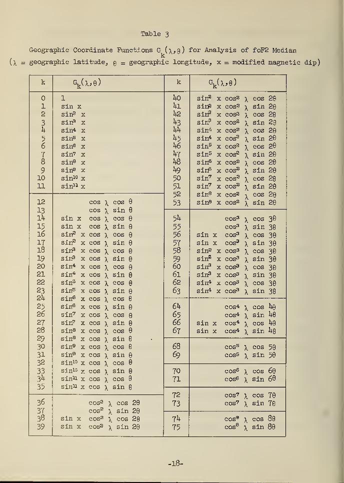
where the geographic functions G, (X, 9) are defined in Table 3. The

coefficients D, are determined by the method of least squares using all

available A-, B-, and C-data for the given hour. The modified magnetic

dip x does not appear in the functional form G, (X, 9), since x is itself

a function of X and 9 (see Section 5)» The variable X has been retained

in the weighting factors involving powers of cos X, in order to provide a

continuous latitudinal variation of the weight factors and to annihilate

-IT-

(x =

Table 3

Geographic Coordinate Functions G (\,q) for Analysis of foF2 Mediank

geographic latitude, 9 = geographic longitude, x = modified magnetic dip)

k \(\,b) k \(x,e)

12

3

4

5

6

78

91011

1

sin xsin2 xsin3 xsin* xsin5 xsin6 xsin''' xsin8 xsin9 xsin10 xsin11 x

4o4i42

4344

4546

47k8

49

50

51

52

53

sin2 x cos2 x cos 20sin2 x cos2 x sin 20sin3 x cos2 x cos 20sin3 x cos2 x sin 20sin* x cos2 x cos 20sin* x cos2 x sin 20

sin5 x cos2 x cos 20

sin5 x cos2 x sin 20sin6 x cos2 x cos 20

sin6 x cos2 x sin 20sin7 x cos2 x cos 20sin7 x cos2 x sin 20sin8 X COS2 y cos 29sin8 x cos2 x sin 2912

13141516IT18

19202122

232425262728

29303132

333435

cos x cos

cos x sinsin x cos x cos

sin x cos x sinsin2 x cos x cos

sin2 x cos x sinsin3 x cos x cossin3 x cos x sinsin* x cos x cossin* x cos x sinsin5 x cos x cos

sin5 x cos x sinsin6 x cos x cos

sin6 x cos x sinsin7 x cos x cos 9

sin7 x cos x sinsin8 x cos x cossin8 x cos x sinsin9 x cos x cossin9 x cos x sinsin10 x cos x cossin10 x cos x sinsin^ x cos x cossinU x cos x sin

54

5556

5758

59606162

63

cos3 x cos 30cos3 x sin 30

sin x cos3 x cos 30sin x cos3 x sin 30sin2 x cos3 x cos 30sin2 x cos3 x sin 30sin3 x cos3 x cos 30sin3 x cos3 x s in 30sin* x cos3 x cos 30sin* x cos3 x sin 30

646566

61

cos* x cos 40

cos* x sin 40

sin x cos* x cos 40

sin x cos* x sin 40

68

69

cos5x cos 50

cos5 x sin 50

7071

cos6 x cos 60

cos6 x sin 60

72

73

cos7 x cos 70cos7 x sin 7036

3738

39

cos2 x cos 20

cos2 x sin 20sin x cos2 x cos 20sin x cos2 x sin 20

74

75

cos8x cos 80

cos8 x sin 80

-18-

functions involving 9, at the geographic poles. This prevents further

ambiguous values at the poles. The variable x could also have been used

in the "weight factors, in place of X, since cos x = 0, when X = ± 90 .

This change could be considered in future work, although its effect would

perhaps be negligible.

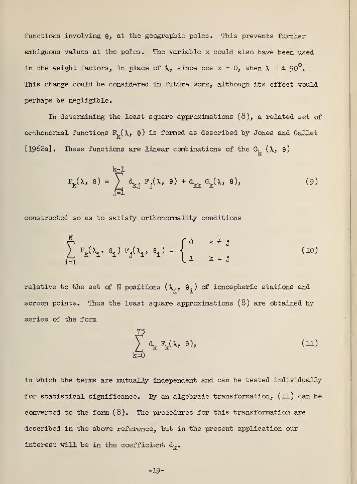
In determining the least square approximations (8), a related set of

orthonormal functions ~FA\, 0) is formed as described by Jones and Gallet

[1962a]. These functions are linear combinations of the G, (\, 0)

k-1

Fk(x, e) = £ \j FjU, e) + d^ G

k(x,e), (9)

3=1

constructed so as to satisfy orthonormality conditions

f (0 k* J

l_Wei)-(Ve1)={i k = j

(io)

relative to the set of N positions (X.> 0.) of ionospheric stations and

screen points. Thus the least square approximations (8) are obtained by

series of the form

75

\ FkU» e), (11)

k=0

in which the terms are mutually independent and can be tested individually

for statistical significance. By an algebraic transformation, (ll) can be

converted to the form (8). The procedures for this transformation are

described in the above reference, but in the present application our

interest will be in the coefficient dk .

-19-

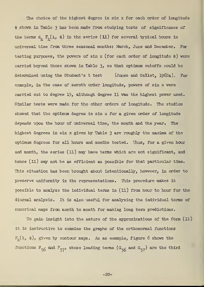
The choice of the highest degree in sin x for each order of longitude

9 shown in Table 3 has been made from studying tests of significance of

the terms d, F, (\, 9) in the series (ll) for several typical hours in

universal time from three seasonal months: March, June and December. For

testing purposes, the powers of sin x (for each order of longitude 9) were

carried beyond those shown in Table J>, so that optimum cutoffs could be

determined using the Student's t test [Jones and Gallet, 1962a], For

example, in the case of zeroth order longitude, powers of sin x were

carried out to degree 15, although degree 11 was the highest power used.

Similar tests were made for the other orders of longitude. The studies

showed that the optimum degree in sin x for a given order of longitude

depends upon the hour of universal time, the month and the year. The

highest degrees in sin x given by Table 3 are roughly the maxima of the

optimum degrees for all hours and months tested. Thus, for a given hour

and month, the series (ll) may have terms which are not significant, and

hence (ll) may not be as efficient as possible for that particular time.

This situation has been brought about intentionally, however, in order to

preserve uniformity in the representations. This procedure makes it

possible to analyze the individual terms in (ll) from hour to hour for the

diurnal analysis. It is also useful for analyzing the individual terms of

numerical maps from month to month for making long term predictions.

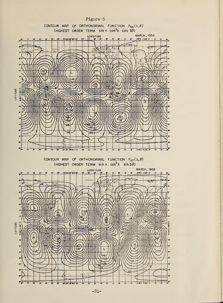
To gain insight into the nature of the approximations of the form (ll)

it is instructive to examine the graphs of the orthonormal functions

Fv(^> 9); given by contour maps. As an example, figure 6 shows the

functions F g and F , whose leading terms (G^g and G „) are the third

-20-

tr W tr ins'

Figure 6

CONTOUR MAP OF ORTHONORMAL FUNCTION F56 (X,0)

(HIGHEST ORDER TERM sin x C0S3X COS 30)

LONGITUDE MARCH, 1958ijy isir Krvavrtsiisy car iiy iff us1 ay Ty w ty w lyicsr o-East ly »• «y tr

'5' tr IDS' Iff US' ISO* B? EAST BO-HEST 165' 1ST U51IB- 105* SO' IS

1 60" «' IS'IEST IP EAST IS" X- Kf

CONTOUR MAP OF ORTHONORMAL FUNCTION F57 (X,0)

(HIGHEST ORDER TERM sin X COS3 X sin 3(9)

LONGITUDE MARCH, 1958

w w tr ids1 iff '» ar its' east wigiic a1 iff bt a1 »r ly ir v v s-iest peast &• jo- «• tr

tr w iff iw isr «jeast b-kst tr isr as1 iff «• so* ry tr w w is'itsi it east iy *r *y

-21-

3 3order longitude functions sin x cos \ cos 3 8 and sin x cosJ X sin 3 9>

respectively. Several additional examples are contained in Appendix B.

Among the properties illustrated are the close relation to magnetic dip

and the position of zeros and relative maximum and minimum points.

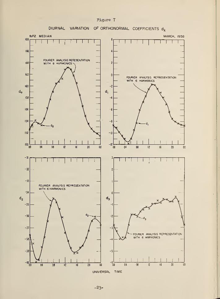
3.2 Diurnal Variation

A numerical map representing "both the geographic .and diurnal

variations of the ionospheric characteristic can now he formed by Fourier

analyzing the orthonormal coefficients d, (k fixed) obtained from the

geographic analyses for the 2k hours of universal time, Typical examples

of these coefficients are shown in figure 7 for k = 0, 1, 2, 3 (March

1958)» Also shown in these graphs are the Fourier representations of the

form

6

d. (T) = a'k

' + \ a\k

) cos jT + b\k

' sin JT|

, (12)

j=l

where T denotes the universal time hour angle ( -180 ^ T ^ 180 , T =

at 12 noon U.T.). Further examples of this type are given in Appendix

C. Only six harmonics are used for this representation since it was known

from previous work [Jones, 1962; Jones and Gallet, 1962a and 1965b] that

at most eight harmonics are needed for the diurnal variation and since

experiments made in this application showed that harmonics seven and eight

gave no significant contribution. The d, have a remarkable degree of

smoothness and continuity over a 2k hour period, in spite of the fact that

the coefficients for each hour are obtained independently. Further studies

have shown that the diurnal variations of the coefficients D, in (8) are

not as smooth as for the V-22-

fbF2 MEDIAN168

164

do

Figure 7

DIURNAL VARIATION OF ORTHONORMAL COEFFICIENTS d k

6

MARCH, 1958

FOURIER ANALYSIS RERESENTATIONWITH 6 HARMONICS "

FOURIER ANALYSIS REPRESENTATIONWITH 6 HARMONICS

CO 04 08 12 16 20 00 04 08 12 16 20 00

-32

FOURIER ANALYSIS REPRESENTATIONWITH 6 HARMONICS

00 04 20 00 00 04

UNIVERSAL TIME

-23-

The numerical map of the ionospheric characteristic can now be

written in the form

75

'(x, e, t) =^T d^ (t) Fk (x, e), (13)

k=0

where the functions cL'(T) have the form (12). For use in practical

applications, q (\, 9, T) is expressed in terms of the simpler functions

Gv (\» 9) in Section 5. Examples of graphical contour maps of foF2 median

for March 1958 computed from q (\, q, t) are shown in figures 8 and 9> for

the hours U.T. = 00, 06, 12, 18. As can be seen, the problem of ambiguous

polar values is no longer present. Also, by comparison with graphical

contour maps from former analyses such as Jones and Gallet, [1965a], it

is evident that the new maps represent more detail in the equatorial

region. Further comparison of different analyses will be dealt with

in the following section.

To conclude this section we shall mention a few of the strong

connections between the various steps of the mapping procedures described

above. The use of a universal time analysis eliminated polar ambiguities

but, at the same time, created another difficulty: increased complication

of geographic variations. To take account of that fact, it was necessary

to use a larger number of geographic functions (including higher orders

of longitude). This placed even more importance on C-data to control

instability; hence more screen points had to be used. Since the geographic

analysis is far more difficult than the diurnal, it was decided to analyze

the geographic variations of the A-, B- and C- data for fixed hours of UT,

-2k-

rather than the Fourier coefficients from the diurnal analysis, adjusted

to UT. The latter approach, though perhaps more desirable from the

viewpoint of reducing the overall number of terms needed to define a

numerical map, would he more complicated since the Fourier coefficients

have extremely different types of variations from one coefficient to the

next. Hence a careful study would he required for each (of approximately

17) Fourier coefficient. Perhaps this is an area worthy of further

investigation.

-25-

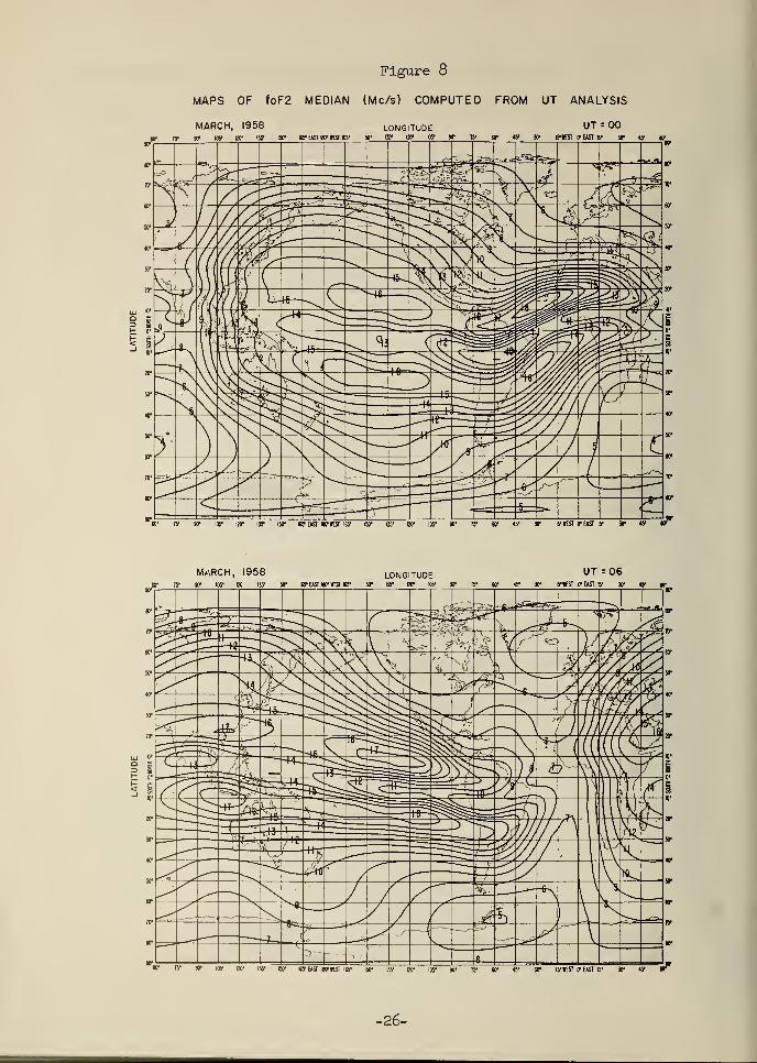
Figure 8

MAPS OF foF2 MEDIAN (Mc/s) COMPUTED FROM UT ANALYSIS

MARCH, 1958 LONGITUDE UT = 00tr w tr IPS' ar 'ff fig 163* east w «st iss- isc iff ar «• sc ry w «y y lyttST ir east ry »• «y y

to- iy ar ice* iv us- iscr *?east

M^RCH, 1958 UT =06W 75- W 105* IZO Iff ISO" »• EAST IKf WEST «• ISO

1 Iff 00" KB1 XT 75" SO" «• ff WIEST 0" EAST 6' »• «• «•_

» » » » Iff ISO*

•26-

Figure 9

MAPS OF foF2 MEDIAN (Mc/s) COMPUTED FROM UT ANALYSIS

MARCH, 1958 LONGITUDE«• is* ac w in- iw im* KyEASTwigng' iso* iiy w *&• so

- ty

UT = I2

<y »• lyKST irEAST 6- » «y «r

MARCH, 1958 LONGITUDEJIT 7S' 30" IW IZO* IM1 ISP 165' EAST Iff «sr W 150* !»• Hr US' XT 75"

UT = I8

45' W lylEST CTEAST 15- »• »? ff

iw !»• ley east wpiest «• isr •»• izo* las'

-27-

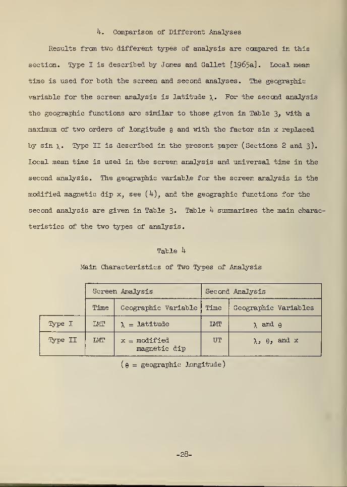
k. Comparison of Different Analyses

Results from two different types of analysis are compared in this

section. Type I is described "by Jones and Gallet [1965a]. Local mean

time is used for both the screen and second analyses. The geographic

variable for the screen analysis is latitude \. For the second analysis

the geographic functions are similar to those given in Table 3, with a

maximum of two orders of longitude 9 and with the factor sin x replaced

by sin \. Type II is described in the present paper (Sections 2 and 3).

Local mean time is used in the screen analysis and universal time in the

second analysis. The geographic variable for the screen analysis is the

modified magnetic dip x, see (h), and the geographic functions for the

second analysis are given in Table 3* Table k summarizes the main charac-

teristics of the two types of analysis.

Table k

Main Characteristics of Two Types of Analysis

Screen Analysis Second Analysis

Time Geographic Variable Time Geographic Variables

Type I LMT X = latitude LMT \ and e

Type II IMT x = modifiedmagnetic dip

UT \, e, and x

( 9 = geographic longitude

)

-28-

For comparison, the two types of analysis have been applied to the

same sets of A- and B-data for the characteristic foF2 median for four

seasonal months of the high and low years of solar activity, 1958 and

195^. For each type analysis and each month, the root mean square (RMS)

residual has been computed using residuals between A- and B-data and

numerical map values for all stations and all 2k hours. The values of

the EMS residual, which estimate the standard deviation of residuals,

are given in Table 5« As can be seen, there is a major improvement in

the representation of the given data. The reduction in the RMS residual

for Type II ranges from 30 to kj per cent. The values of the RMS residual

Table 5

RMS of Residuals of (Mc/s) of A- and B-data for Two Types of Analysis

(All hours and all stations of foF2 medians)

195^ 1958

Analysis Mar. June Sept. Dec. Mar. June.

Sept. Dec.

Type I •72 .58 .69 .66 1.10 1.06 1.09 .98

Type II .38 .36 .kl ,k2 .63 .59 .60 •67

in Table 5 for Type I are considerably higher than those reported in the

previous paper [Jones and Gallet, 1965a] . This is due to the use of about

30 additional B-data stations. The number of stations with A- or B-data

and the number of screen points for each month used in the present study

are summarized in Table 6.

-29-

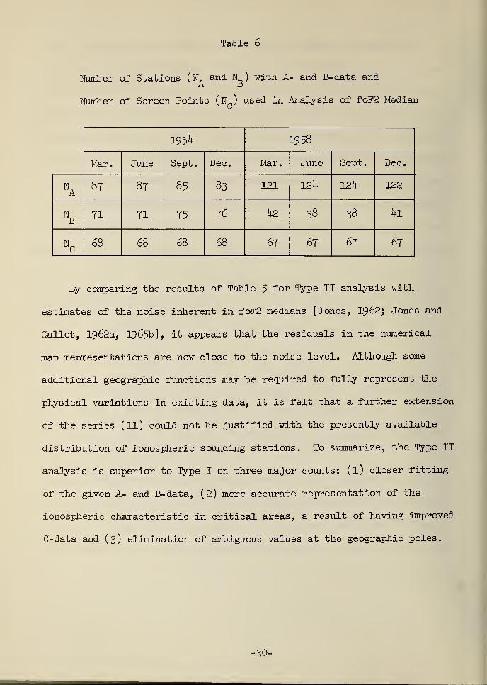
Table 6

Number of Stations (n. and H_) with A- and B-data and

Number of Screen Points (N ) used in Analysis of foF2 Median

1954 1958

Mar. June Sept. Dec. Mar. June Sept. Dec.

NA

87 87 85 83 121 124 124 122

NB

71 71 75 76 42 38 38 41

Nc

68 68 68 68 67 67 67 67

By comparing the results of Table 5 for Type II analysis with

estimates of the noise inherent in foF2 medians [Jones, 1962; Jones and

Gallet, 1962a, 1965b], it appears that the residuals in the numerical

map representations are now close to the noise level. Although some

additional geographic functions may be required to fully represent the

physical variations in existing data, it is felt that a further extension

of the series (ll) could not be justified with the presently available

distribution of ionospheric sounding stations. To summarize, the Type II

analysis is superior to Type I on three major counts: (l) closer fitting

of the given A- and B-data, (2) more accurate representation of the

ionospheric characteristic in critical areas, a result of having improved

C-data and (3) elimination of ambiguous values at the geographic poles.

30-

5. Application of Numerical Maps

5.1 Simplified Expression of q (\, 9, T)

As an aid to evaluating numerical maps, this section reduces the

function q (\, 9, T) to a form expressed in terms of the geographic

functions G, (\, 9). Also included in this section are the formulas

necessary for calculating magnetic dip I. To obtain increased generality,

so that the discussion will apply to numerical maps of any ionospheric

characteristic, we introduce a set of geographic functions G, (\, 9) in

Table J, of which Table 3 is a special case. Here the integer q.,

i = 0, 1, ..., m, denotes the highest power of sin x for the i order

harmonic in longitude, and m denotes the highest order of longitude.

The parameters q. and m may change from one ionospheric characteristic

to another. However, the general form of the numerical maps will remain

fixed. For indexing purposes it is sometimes convenient to introduce

the sequence k., i = 0, 1, ..., m, such that G (\, 9) is the last of1 j£ .

th1

the geographic functions of i order longitude:

Gk (x, 9) = sin^xo

cii ±G (\, 9) = sin x cos \ sin ig, i = 1, 2, ..., m. (1*0K..1

Thus

% = V q±=

kj-

"kj'

1, i = 1, 2, ..., m, (15)

and the total number of geographic functions in Table 7 is given by

K + 1 = k +1 .

m

-31-

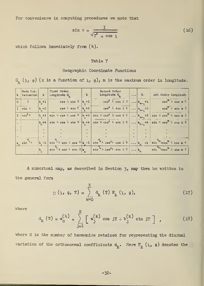
For convenience in computing procedures we note that

Isin x =

^I3 + cos \

which follows immediately from {h).

(16)

Table 7

Geographic Coordinate Functions

Gt (\> 9) (x is a function of \, 0), m is the maximum order in longitude,

k

Main Lat

.

Variation k

First OrderLongitude G, k

Second OrderLongitude G, k mth Order Longitude

1 k +1 cos X cos 8 k +1l

cos3 X cos 2 8

• • •

k +1m-i

k +2m-i

k +3

k +4

k -1m

cos X cos m 8

1 sin X k +2 cos X sin S k +2l

cos2 X sin 2 8 cos X sin m 8

sin X cos X cos in 8

sin X cos X s in m 6

2 sin X k +3 sin X cos X cos 9

sin X cos X sin 8

qsin 1 X cos X cos 8

k +3l

k +4l

k -12

sin X cos2 X cos 2 8

...

k

k +4

k -11

sin X cos2 X sin 2 8

qsin °X

qgsin X cos

2 X cos 2 8 sin Xcos X cos m 8

k1

4sin X cos X sin 6 k

s

4sin

SX cos2 X sin 2 8 ... k

msin Xcos X sin m 8

A numerical map, as described in Section 3> may then be written in

the general form

K

Q (\, S, T) = \ d^ (T) Fk (x, e),

k=0

whereH

^ (T) = a^k)

+ ) fa(k)

cos jT + b(k)

sin jT

j=l

(IT)

(18)

where H is the number of harmonics retained for representing the diurnal

variation of the orthonormal coefficients cL. Here F. (x* 0) denotes the

-32-

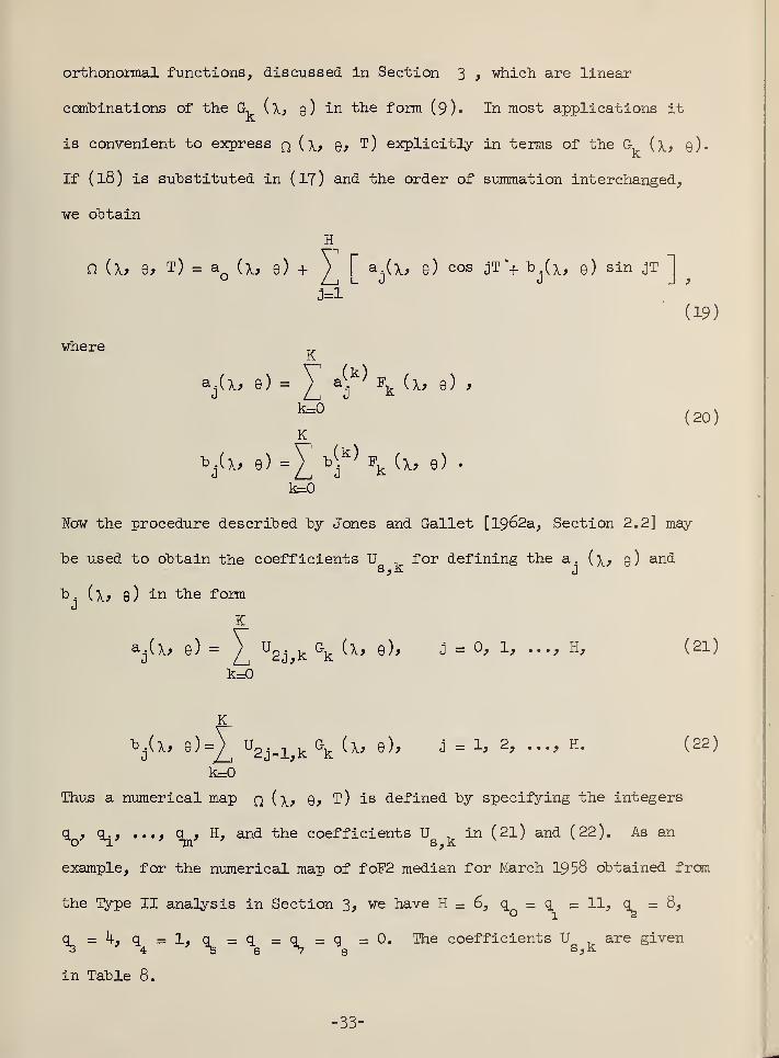
orthonormal functions, discussed in Section 3 , which are linear

combinations of the G. {\, 9) in the form (9). In most applications it

is convenient to express q (\, 9, T) explicitly in terms of the G, (\, 9).

If (l8) is substituted in (IT) and the order of summation interchanged,

we obtain

H

Q (\, B, T) = aQ (\, 9) + \ 1 a^(x, e) cos jT *+ b (\, 9) sin jT

3=1

(19)

j t

whereK

aj(x, e) = ) a^k)

Fk (x, e) ,

16=0(20)

K

b.(x, e)=£ *(/°\(^ e) •

k=0

Now the procedure described by Jones and Gallet [1962a, Section 2.2] may

be used to obtain the coefficients U , for defining the a. (\, 9) and

"b • ( Xf 9 ) in ^he formJ

K

aj(x* e) = V u2^ k

Gk (x, e), J = 0, 1, ..., H, (21)

k=0

K

Dj(\, 9)=^ u2j-i,k

Gk (^ e) > J = X>

2, •••» H - ( 22 )

k=0

Thus a numerical map q (x, Q, T) is defined by specifying the integers

9. 9 <!*> ••*> q, H, and the coefficients U in (2l) and (22). As an

example, for the numerical map of foF2 median for March 1958 obtained from

the Type II analysis in Section 3, we have H - 6, q = q = 11, q = 8,

a = kj q = 1, q = q =q=q =0. The coefficients U are given

in Table 8.

-33-

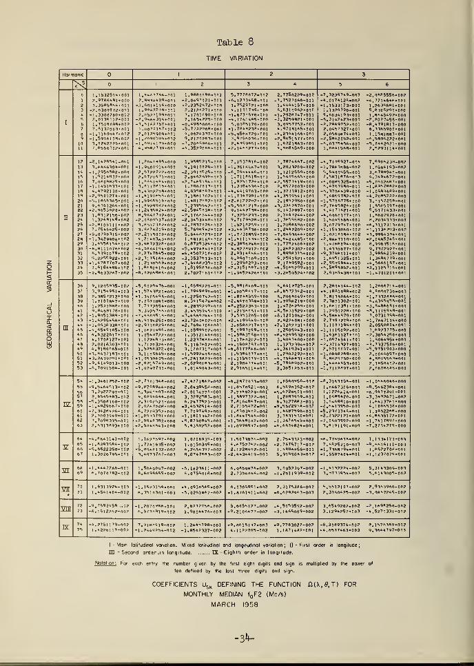
Table 8

TIME VARIATION

1.1532.9783.358

-2.O30-1 .3302.0131.7S17. "13

-1.116-1.5913. 024"'.055

2514*0016481*0005864*00]0872*om8700*0028112*001Bo9B.o022003*0010Q47.nnjhlO».O0?2225*0016302*001

-3.60 ] 6 1 16

-3.61 .02.0

6771966*311*775

•001

•Oil

'000001001oo 1

•001

002001

1 ,988oo9o-ool-?. 0497021-001-7.2352*72*0002.212*271 *0007. 1701 090*0007.1654275*000

-8.4988no**000-5. 7772968. O ol4.0624337*0009.2120283.001

-7 ,2066066-001-4.35?9oo*.nol

-1.7-5.9

77B072-002233468-001529721 .0001 1 739*000730S7fl*001761405. 000085170*001

23B.001S6a7?g*00175*036*001369061*001

273.001

2.775o2?9.-3.7527066-1.4444)57.8.63109*2'

-1.292B747.-3.3259921.3.6957762.4.97081*5.

-4. 23441*6.-2.965)677.

1 .6721863-4.9686569.

-7.3239749.-4.017412B.-1.1533173<

1 .1329790-9.60J4193--5.3142423.-2,286975?.2.0457327.2.0569B74.-2.5B42052.-6.0376456.

1 ,0ft41 568.

003002000001000000001001001001

0001)01

-2.0885556--4.771464ft.

1 .2638681-5.8306790.1 .B645492.

-7.8027468.-B.4791B13"6.3365900'1.15B1BB3.

-6.5B96222.-5.0442021

.

2.52931 14.

002

001001000000ooi000001001ooi000001

2223

2728

30

-2.1428541.3.6468304-

-1 .29505B2.I.9214B32"

7.060BU29.-1 .1451633'4.4792)30.

-2.9501274.-5.1B68385<9.4361264.

-2.9653920.1 .B312156.1 .3248J49.

-?.B105111<7. '546425.

-5.0790315"-1 .3929906^3.45581S4.

-8.811 1076-6.3390079.5.2255922.

-1 .47877Q7.3.6184486.

-2.8633267.

.9S01'>16'

.67222V?.

.672167].

Ml' M6.8.4302258

-1 .4)91655-1.59655)6-

1 .8929982-1 .24359248.966779?

-2.0BOO5373.86173a?.3.8B74219

-2.21150004.21403*3

-3.4B7732B'-4.5B64194'2.2747645.

-2.3175164-1 .21305681 .86804)6.

-8.02058B*

00000000)00)00)000

00200100200200200200200200200200200200200)

1 .95882)5.4.191002B-

-2.39)0525.?.04*?696.

-?. 74*9154.1 .780701 3.

4.8358BB7.3.186130?.1.4B1?"B?.3.2396542.

-2.5945038.-2.176*544.-2.3453440.-3.783702*-5.769*94?.5.6448723"1.491816'"6.8729324.-5,497484]

.

-6.4507710.-3.3537013.-3.6468?35.

1 .8)95830.2.70271*1-

7.153781*.-1.351*8*7.-6.7944446.1.7118*,fl.

1.9?5I7?4.1.338463*.

-4,4419703--1.73479B].-2.6)2??o?.-5.5081219.9.144?73Q,7.329*233.9.71 79*28.1.52ia?69.

-3.4438736.-1.7730859.-1.4))1434.-2.389o?46.4.827M9) 2.

2.9314B66.6.9907)09.).295»293.

-2.31518B7.-1,9*5?4?*.

00?OOI

000001ooo001000001OOI002001002001002001001001002001

7,78746*7.3.2033209-1.1212659.). 64056*5.

-2.55774J9.2.867?003.

-). 37)3912.-4.3809541.2.189?950.

-3.3?*?870.6.143?997.2.7647244.

-1 .3*65582.1.2088690.

-1.2942209.-7.0463644.-9.4466695.-1.779?406<1.2*82302.7.B99R375.9.?59]8?1.9.1749592.

-4.51*5299.-3.2*59524.

-4.71 06927.-1 .7863586-6.6400656.7.5831876-

-*. 0085325-6.6763980--8.3708439.7.48*9782--1.6706775.-2.7*45924.4.4173621--4.6060177.

1 .6045666.3.0779747.

-1.1543060.1.0?18)B4.-2.9867110.

1 .4768094-1.433SB77.

-9.3748011.1.6951325-

-2.9509844.-6.5898852.2.9369438-

002001003001001000000000000001onl00100000200200)00000200)001000001001

7,6906238.1 .0564193-3.67BB940.4.349467?-

-6. 0512687--1 .B957BB2--1 .06B3689.-4.208822?.3.015728a-

1.8666097.

6.5171433.1.B607920'a. 2034333--6.31173)3--1. 1136293--3.9964334--2.08B6346-8.9963518-9.7372977-3.9856239-) .3696779.

-4.5666187.-3.1108716.-1.4701201-

00200200100100100000100000100100100100000100200100100100)00)001001001001

4142

9.1205935-3.9154951-2.3857212-1 .7100R47-1. 7573888-9.8468178-

-1 .9051389--1 .6295466--1.0938338-.4.8549185.4.6322617.4.1708127-2.0218303-4.9)80065--3.8437183--3.2639201--9.4149013.-8.7091504.

-5. 6029476.•1 ,5743820--1 ,3406498-7.7871880-7.7172664.3.3978766.-7.4860518--6.4094280--2.971 r-829-

-1 .1621496,1 .054072?"1.177*833.4.7170376.1.60503??,

3.110864b.-1 .0510605--2.6216749.-1 .0797730.

001

001001001OOO000001000

000001001001

000001001

-1.6594??].-1.7949890--1 .225074?-R.34)6o?6-4.2839799.3.4535946.

-3.4660744.-3.7240602.-2.7684700.-1 .0899902.1.3512140.1.2237B80.5.1167602'3.1707317.

-1 .5992406.-9.2B13B29.-2.6290183.

1 .0149043-

-5,991 8409.-1.0058617.-1 .B74B5S9.-2.B470369.-8.2527363.-1.2156061.7.5363205.-2.4199649.3.0580217"5.0997099,-1.5963580.1.1760202.-4.180O7B7.-6.8177866.

1 .5384077.-1.1158079.2.1904774,2.9166] 14.

001

000OOO001000001000000001001001001001001

00)001

8.64)7725.-6.6572342-8,2068049-

-1.705r219-1 .4726269.

-8.6631529.-8.1201062-2.8224081"

-7.1267731"3.2606943,

-8.4?49S32"3.8043400"1.1232394"

-4.3619341.1 .2902292'

-4,7548831..5,7948902.2.3051263.

2.28041 44.

-4.18B109B.7.8)38066.2.3B71302-

-1 ,**1039l.1 .2951228-

-8.5B64879-2.7397279.1.1107195.

-1.1115097.1 .4361127.

-1 .0674541.-2.3714327.2.6710037.

-1 .0848289.8.8679750'1 .4484B53.

-1 .71 17B97.

00200200100100000000000000100100100)00)001001000001001

1.2066214.4.B060730--1.7332886-4.6345958--3.8486681--8.1115969-7,0731768.

-1.76671 14.

2.0558804-3.8923775.

-2.3054260'1.5064954.

-3.7337506--6,9751903-2.0044097-4.8016563.2.185O407.7.0*78686-

001

003001001000001001000001OOOOOO000001000000001001000

IE

-1 .3461782-002-9.5464613-0023.3922297-0012.6545463-002

-6. 3508100-00?-1 .4929667.000-7.3428426-0017.3003949-0017.7096396-0017.6313893.000

-2. '301 348-001-9.87OB944-0026.3060403-0024.6890644-0012.3100620*0002.0267526.0006.7209352-001

•1 ,0933791 .000•2.9948 382.000.7.6040843.000

-7.4771887-00?2.8439556-001

-2. 0136770-00!3.3292683-0016.2477823-00]

-3.46326)4.0007. 7097492-00)

-) ,)B0)342*O0O-fl. 8750945-00)5.4389282*000

-6.2877033-002-).857o921-0032.7749279-001'.). 8897377.00)7.8]648a7-0012.7156472-0011.8303902-002

-1 .8447846-001-1 .3648)02.000-1 .0998937.000

] .0560956-0026.5890352-002

-6.4229601-0011,2083959-0016.31278B3-001-9.5622918-0021.46B7696.0003.3831630-00)

-).367*5»b.O00-4.6834824-00)

-8,3)63058-001

] .0667306*0001.1224r1(S-0011 .06B942O.0OO3.64698)0*000-2.64) 3950*0005.23^3348-001•2.2322121*000-7.0603997.0003.8J91 J90.000

•1 .0646046*000-8.5462384-001-6.0437391-001-3. 3497671-00?

1 .6413761*0004.1 006838*0001 .085226B.0O0

-4.B635177-001-1 ,7417897*000-7. 2734279. OOO

-4.8641 141-002-1 .8283684-002-8.6522250-0021.3026795-001

.1677597-002

.774]635-002

.0960132-002

.4073767-003

1 .0706939-0031 .0150306-0014.2854347-0028.8747SO3-002

1.6073676-0024.6752752-0022.1226492-001-2.4434419-003

2.7543373-00?-2.76767] 7-00?1.4B86456-00)5.9)89883-00?

-6.7769638-0027.6B252)0-003). 7368794-00)-1 .5587404-00)

) .1334173-003-9.66)61 11-003

1 .8822708-001-). 1237079-00)

21-1 .4447260-0016.7078782-002

1.5069047-0028.6098689-002

-5.182361 1-0024.07560] 8-O02

6.9669676-0022.7354046-002

3.0957397-002-1.20H939-O02

4) 37224-0021733954-003

5.3143309-0036.6)43006-00?

¥H ] .6313974-0031.4541404-00?

-1 . 1573154-0018.36)0301-003

-4,09305*6-00?-5.026)067-002

6. 0306951-002-) .876)9) ]-002

2.3)76386-002-6.62929*3-003

6.5612)07-002 2.9 3*3960-00?7.3760425-002 -3.06*7246-002

VIA-4. 7892458 .,02

-6.16)2262-002-1 .2070486-0016.573n6]9-002

2. 6237786-00?1 .9004476-003

5.6056177-002 -4.6053592-002-9.2106477-002 -3.1466009-002

3.6549202-002 -2.1698250-0023.1294257-003 -4 .5270 331 -002

rx-4.2751179-002

1 .42761 17-00?7.91009)9-00?

•I .2444754-002] .2446798-001

-1 .8567377-00?-9.0615137-003 -9.7783027-00?4.1127705-002 1.1871482-001

5.3089374-002-4.6637463-003

2.1576389-0029.3644797-003

I - Mam latitudinal variation. Mixed latitudinal and longitudinal variation; II - First order in longitude;

HI -Second order, in longitude IX -Eighth order in longitude.

Nototion: For each entry the number given by the first eight digits and sign is multiplied by the power of

ten defined by the last three digits and sign.

COEFFICIENTS USK DEFINING THE FUNCTION fi(X,0, T) FOR

MONTHLY MEDIAN f F2 (Mc/s)

MARCH 1958

-3^

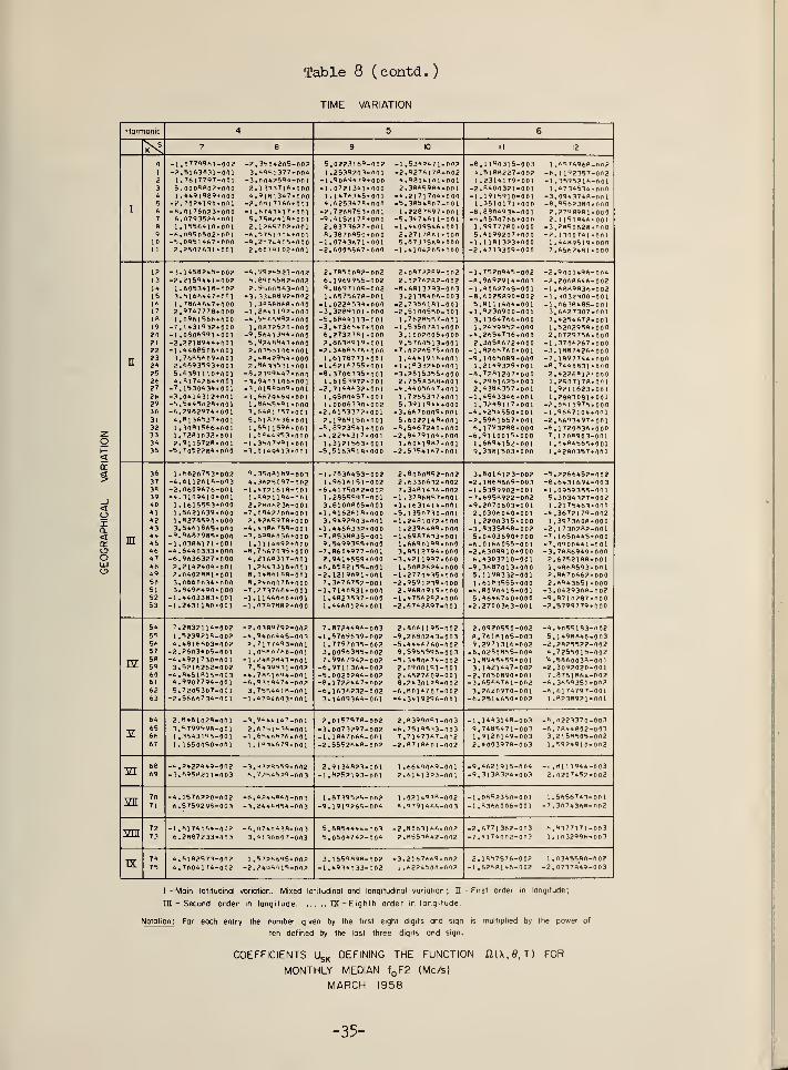
Table 8 (contd.

)

TIME VARIATION

10

.0779961-002

.6163831-001

.7617707-00]

.0008802.000,449i989+ooo,7o24j9o.ooi.0176023*000.0793524*00).]6564io.ooi,o96o502*ooi.095)467*000.2507631.001

,36o42o5-oo?.496] 377-004. 0042594-001. 1 337716*000.9l«l347.OO0.001 7166*00

1

.6743417*001

.76874)8.001,l?667o?.001.S7R 1 004*001.2074405*000.60701 02*001

5.0223169.1 .2539203.

-1.9069479.-1.0721341.1.1476345'4.6253470.

-2.7268753--9.4152178.2.9373627.B.3B70BSO.

-1 .0743671.-2.6005567.

-1.5342471-002-2.9276178-0024.9B041OJ-0012.3865984-00]

-4.2171704*000-5.3854807-0011. 2287897. 001

-5.347461 1-001-1 .4409546.0012.2717B61 .0005.97J3569.000

-1. 4104205.000

-8.1190315-0034.518B227-0021.2314179-001

-2.B400321-001-1 .19159] 0-001

1 .3510171.000-8.8R04934-001-4.0530766*000

1 .9977780*0005.4099207*000

-1 .1 181323*000-2.4713309*000

1 .6576968.002-6.1 192357-002-1 .3596216-001

1 .4734534.000-3. 0943748-001-8.9662380.0002.27989B1.0002.118)846.001

-3.285062fl.oo0-2. 1300741*001

1 .4489519*0007.6562481 *000

<IQ_<or

O

- 1. 1458745--2.2159441-1.6053418-3.5166447-1 .7864647.2.974777B.1.0961566.

-7.1431932.-1 .0806991.-2.2218944.-1.4468506"3.7685609.2.6693593.5.63811 10<4.A174284.-7.1530434.-3.0414312<-5.5445028.-6.2982974.4.B]36537.

1 .3081566.1 .7281032.2.9H572B.-5.7Q52284.

002002002001

000000000000001001001001001001001001001001001001001001001ooo

-6.99?*.523-6.8906682-2.9600663-

-3.3348892-1 .3066868.

-1 .2841192.-4.666690?.1.0872520-

-9.5641394.5.924BH43.2.0365106'2.4842964.2. 8633531-

-8.2399447.-3.9411 106'-3.0168509.-3.6679469.1.8666491.3.6481 757,5.6]87436.1.661 1596.1 .6644053,

-1 .3607991.-3.0] 494 1 3.

2.7850082-6.1969955-9.86971 06-

1.657567B--1.022«534.-3.3289101.-5.6844113--3.4736647.6.27327B1

.

2. 86389)9.-2.346H676.

1 .617B77]

.

-1.62)6765.-8.3706335"1.6153972.

-2.9144632.1 .9500457.1 .0006330.

-2.615337?.2.1969]50.-8.892364]

.

-4.2244317.1.3121563.

-5.5163618-

002002002001000000001000ooo001000001001001001oni001002001001000001001000

2.0872289.2.02762P2-

-B. 6813793-3.2136406.

-2.7356181.-2.5100560.

1 .7628657.-1 .5350781

,

3.1002005.9.57605] 3-

-7.0226575.1.4441918.

-1. 1°33240.-3.2815365.2.756B368.

.4.4406647,1 .7266337.5.391 1944,

-3.6670009.5.602214A,

-8.5467240,-2.8479104,1.604)987,

-2.5354167.

-1.7620945.-8. 9692914--1.4062745--8.6025890-5.8111404.-1,9230900.3.1364766.1.2499962

-4.2654736.2.3058672

-1 .B266760'-9. 1066089.1.2149329.

-8.72B1207.4.2961625.2.4386357.

-1.4543346.1.3248] 17.

.4.4264550'-2.5961657-6.1793288.-6.9H0015,1.6694152.9.3381503.

002003001002001001000000000000001000001000001001001001001001000000001000

-2.9001496--2.2068646--1 .6689836--1 .3032300--1.0638485.3.6627307.3.4254672-1 .5202958,2.0729766.

-1 .3706267.-3. 1B87426--7.1897744.-8.7440831-2.4226812'1 .2607178.1.9211623.1 .2883081 •

-2.06] 0975.-1 .9667104.-2.6693497.-6.1720B36.7.1708903-1 .0484565.1 .4280357.

002002001001001001000000000000ooo000000001001001000001001000001001001

m

1.6620763--4.6112616--2.0609676'-4.3109410'1.1615553'1 .56216391.8278590'3.5461865.

-9.9687985'-1 .03881 71'

-4.6440333--6.9636327-2.2142404'2.0402881'3.0660034-3.8498490-

-1 .4403383--1.2431 180-

002003001001000000000000000001ooo000001001000000001001

9.3608169.4.3625097-

-1.477161 A-

1 .8621 194-2.2x06236-

-7.0842'00-2.4266978.

-4.4386768--3.B9O6056'1.1] 14892'

-8.7667035-4.216P317-1 .2843316.8.048M 08-

8.24*0076.-7.2737664--1 .1166680.-1.0787882.

-1.7836453-1.96161S1-

-6.4176082-1 .2856697-3.8100805-

-1 .4162618.3.9492903--1.4466332--7.8538835-9.5499365.-7.8604977-2.9414659.-6.65B2165.-2.1219091.7.3676752--1.7140831.1.4823637.1 .4460124.

002002002001001000001000001000001000001001001ooo000001

2.Bo6o862-2.6330632-7.3481416-

-1 .3786857--1.1631414--5.1350730--1.2481072.1.2396489.

-1.6987633-1 .6690199.3.A512794.

-3.4211997.1 .5082624.

-1.2770435.-2.9591239.2.9680919.

-1.4756202.-2.6742897-

3.8016123--2,1868669--1.5399902--7.6958922'-9.2070603-2.0306040-1.22003)5.

-3.8335868-5.0403690'-6.0166065.-2.63O9910"6.4303710--9.36S7013.5.1 198332-1.6183655.

-4.8090416-5.4646740"-2.2700363-

002003001002001001000002000001000001000001000001000001

-5.2266452--8.6431694--1.0959355-5.3034327'1.2175463.

-4.3672179.1 .3973608.

-2.17302A2--7. 1 650445--7.0900441.-3.7886949.2.6752188.1 .4868593.2.B670662'2.6943651.

-3.0429308.-9.87] 0287,-2.5799779.

002003001002000002000001000001000001001000ooo002ooo000

nr

7.28321 14-0021 .5239218-0024.4816603-002

-2.2603405-001-4.4921730-0013.5216262-002

-4.8451816-0034.9907794-0015.7206307-001

-2.5666734-001

-2.0389792-002-4.9400445-0032.7177493-0011 ,058nf60-001

-1.2482843-0017.5439931-00?

-4. 7801604-00]-6.9308474-0023.7554418-001

-1 .4704603-001

7.8724406-003-1.6769639-0021.7797035-0023.0096385-0027.9967942-002-6.9711364-00?-5. 0020704-00?-8.1772447-002-6.1636232-0023.1409364-00!

2.806] 195-002-9.26B0243-003-5.4446760-0028.5966596-003-5.3480674-0022.0900]5]-0012.6827609-001B. 2430128-002-6.8016707-002-4.3419296-001

2.0920650-00?8. 7618165-0039.297] 316-002-6.0280865-004-1 .8945459-0013.1421447-002

-2. 7050890-001-3.6666761-0023.2620970-001-6.2514650-002

-4.4055183-0025, 1498840-003-2.282S622-0024.7256015-002'4.5860038-001-2.3092020-0017.8751864-002

-6.3669351-002-6.6174797-001

1 .8238921-001

m

2.8461028-0013.5799998-0011 .3643195-0011 .1660050-00]

.7,9644147-0012.6751«36-00]

-1 ,6640676-0011.1814679-001

7.0157678.002-3.0073297-002-1.1847066-001-2.5552640-002

2.8399061-003-6.7519633-0037,7147367-002-2.B71O6O1-002

-1.1443148-0039.7486471-0031,9120149-0032.4003978-003

.0223370-003

.7844802-003

.2150505-002

.6924910-002

-4.2422449-002-3.695821 1-003

-3. -.370559-0026.7?645?9_oo3

2.9134823-001-1.8252193-001

1 .6649069-0012.614) 373-001

-9.4621915-004-9.3138324-003

-.-..81 1 1944-0032.0207452-002

SR•4.1576220-002 -H. 4746860-0036.5759298-003 -3.2448864-003

1.6739626-002 1.0214918-002-9.1919266-004 8.9791466-003

-1.OS52350-001 1.5656743-001-1.8366006-001 -7.3074368-002

WT -1.6174064-00? _6,07404?8_0036.2887233-003 3.4)30607-003

5.6854444-003 -2. 80b31 66-0025.0504742-004 2.8563642-002

-2.677)362-003-7.4)74002-003

6.8377171-0031 . 1032996-003

IX4.61A2573-002 1 . 57?O695-0074.7004174-002 -2.24060)5-002

3.1569A9O-002 -3.2167669-002-1.4934033-002 , .6274500-00?

2.1867676-002 1.0 345580-002-1 .6266146-002 -2.0737849-003

1 - Main latitudinal variation. Mixed latitudinal and longitudinal variation; U - First order in longitude;

HI - Second order in longitude EX -Eighth order in longitude.

Notation: For each entry the number given by the first eight digits ond sign is multiplied by the power of

ten defined by the last three digits and sign.

COEFFICIENTS USK DEFINING THE FUNCTION n(X,/9, T) FOR

MONTHLY MEDIAN f F2 (Mc/s)

MARCH 1958

-35-

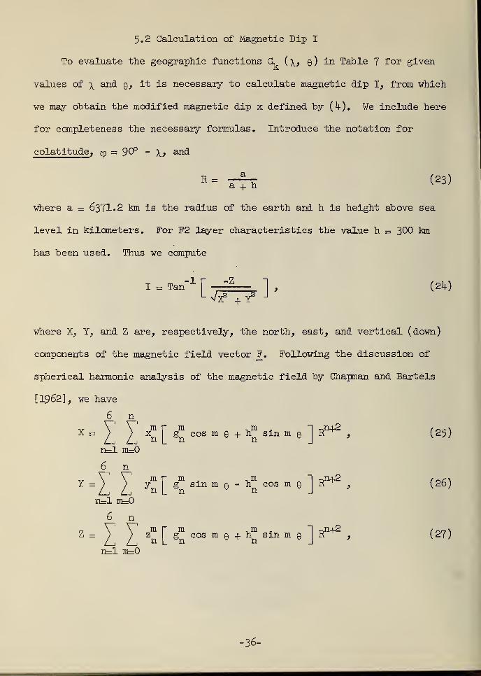
5.2 Calculation of Magnetic Dip I

To evaluate the geographic functions G, ( \, 9 ) in Table 7 for given

values of \ and q, it is necessary to calculate magnetic dip I, from which

we may obtain the modified magnetic dip x defined by (h). We include here

for completeness the necessary formulas. Introduce the notation for

cplatitude , cp = 9°° - \? and

R =a

a + h

where a = 6371-2 km is the radius of the earth and h is height above sea

level in kilometers. For F2 layer characteristics the value h = 300 km

has been used. Thus we compute

(23)

I = Tan-1 r -Z

Wf+y2 J(210

where X, Y, and Z are, respectively, the north, east, and vertical (down)

components of the magnetic field vector F. Following the discussion of

spherical harmonic analysis of the magnetic field by Chapman and Bartels

[1962], we have

6 n

X -T.T.*n=l m=0

6 n

Y-j: >: *n=l m=0

6 n

Z>; >: <n=l m=0

m , m5 cos m Q + h sin mn n

m , m1 cos m 9 + h sin mn ° n

RP+2

m , m 1 r.n+2g sin m 9 - h cos m 9 R^ ,n n J

R,n42

(25)

(26)

(27)

-36-

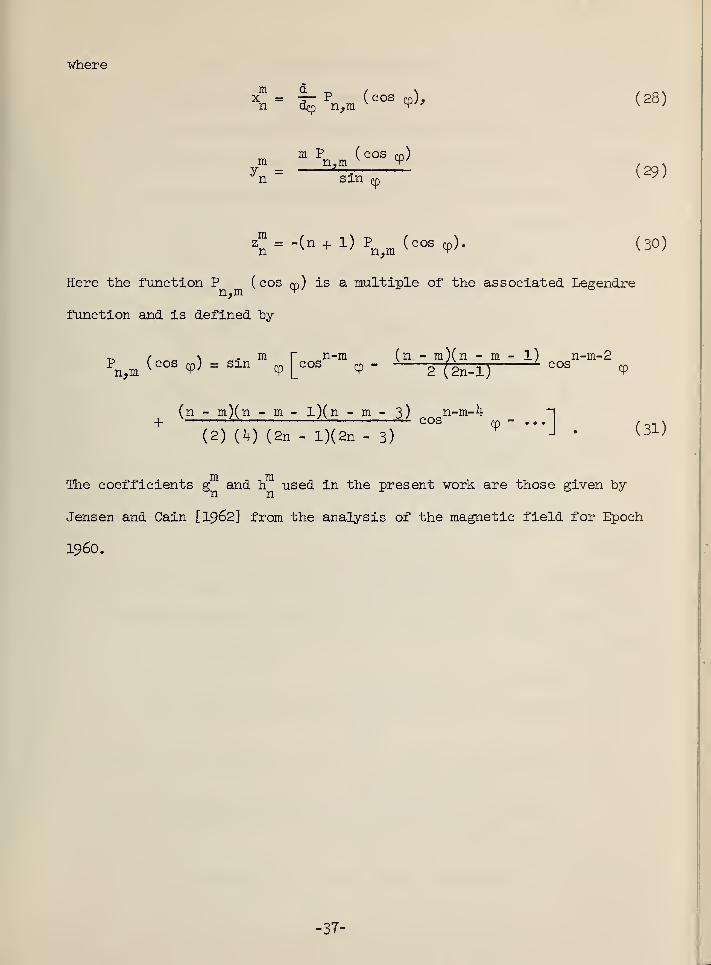
where

x = — P (cos m), (28)n dp n,m ^" v '

m P ( cos co )m n.m ^ ^'yn= 'HT^ («)

mz = -(n + l) P (cos m). (30)n n,m ^ \ -> /

Here the function P (cos m) is a multiple of the associated Legendren,m

function and is defined hy

~ 1 \ . m r n-m (n - m)(n - m - l) n-m-2V ( ^ = ^ VlCOS * 2 (2n-l)icOS

cp

(n - m)(n - m - l)(n - m - 3) n-m- h+

1 ° " m^ n:m

: 1^ n " m ~ 3; cosn-m- 4

_ . 1

(2) (It) (2n - l)(2n - 3) " * ' J '(3l)

The coefficients g and h used in the present work are those given byn n

Jensen and Cain [1962] from the analysis of the magnetic field for Epoch

i960.

-37-

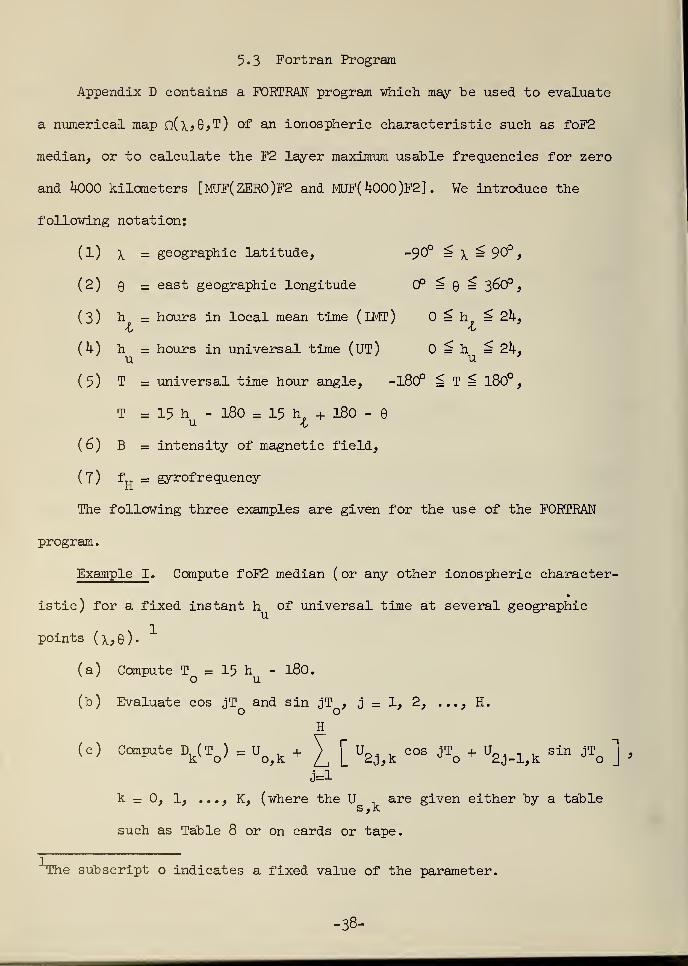
5.3 Fortran Program

Appendix D contains a FORTRAN program which may be used to evaluate

a numerical map q(\>6jT) of an ionospheric characteristic such as foF2

median, or to calculate the F2 layer maximum usable frequencies for zero

and ij-000 kilometers [MJF(ZER0)F2 and MJF( toOO )F2 ] . We introduce the

following notation:

(1) \ = geographic latitude, -90° ^ \ ^ 90°,

(2) q = east geographic longitude 0° = 9 = 3^0°,

(3) h = hours in local mean time (IMT) ^ h ^ 2h}\, '{j

(h) h = hours in universal time (UT) = h = 2k.u u

(5) T = universal time hour angle, -l80° ^ T ^ l80°,

T = 15 h - 180 = 15 h + 180 - 9

(6) B = intensity of magnetic field,

(7) ftt = gyrofrequencyh.

The following three examples are given for the use of the FORTRAN

program

.

Example I . Compute foF2 median ( or any other ionospheric character-

istic) for a fixed instant h of universal time at several geographicu

points (\,6).

(a) Compute T = 15 h - 180.o u

(b) Evaluate cos jT and sin jT , j = 1, 2, . . ., H.

H

(c) Compute D^) = U^ + £ [ U^ cos JTq+ U^^ sin JT

q ] ,

j=l

k - 0, 1, ..., K, (where the U are given either by a tables , k

such as Table 8 or on cards or tape.

The subscript o indicates a fixed value of the parameter.

-38-

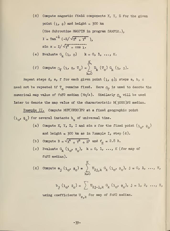
(d) Compute magnetic field components X, Y, Z for the given

point (\ f 9) and height = 300 km

(Use Subroutine MAGFIN in program SAMPLE.)*

I = Tan"1

( -Z/ n/x2 + Y2 ),

sin x = 1/ Vl2 1 cos \.

(e) Evaluate G, (\, 9) Is. = 0, 1, ..., K.

K

(f) Computefy (x, 9, T

Q) =Y \ (T

q) G

fe(\, e).

k=0

Repeat steps d, e, f for each given point (\, 9); steps a., "b, c

need not he repeated if T remains fixed. Here q is used to denote the

numerical map value of foF2 median (Mc/s). Similarly n "will he used

later to denote the map value of the characteristic M(3000)F2 median.

Example II. Compute MUF( ZERO )F2 at a fixed geographic point

(\ , 9 ) for several instants h of universal time.

(a) Compute X, Y, Z, I and sin x for the fixed point (\ , 9 )

and height = 300 km as in Example I, step (d).

(h) Compute B = ^X3 + Y3 + Z2 and fH

= 2 - 8 B -

(c) Evaluate G, (\ } 9 ), k = 0, 1, ..., K (for map ofJ£ O O

foF2 median).

K

(d) Compute a^ (\Q, qq) = ) Ug^

kGR (\q, qq ), 3 = 0, 1, ..., H,

k=0

h. (V e ) = JTu2 ._1A

Gk (XQ, e o ), J = 1, 2, ..., H,

using coefficients U for map of foF2 median.S «J£

-39-

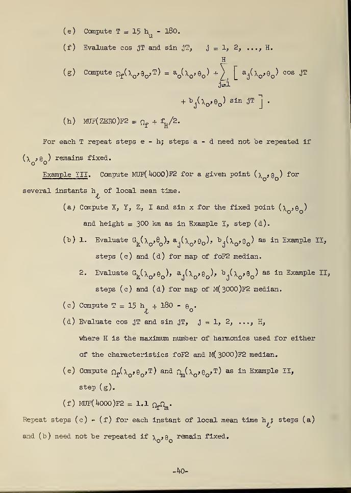
(e) Compute T = 15 h - 180.

(f) Evaluate cos jT and sin jT, j = 1, 2, . .., H.

H

(g) Compute Qt(\ of Q ,T) = aQ(\ >QQ ) +) |

aj(X ^9 ) cos jT

+ bj(X ^9 ) sin JT j.

(h) MJF(ZER0)F2 =Qf

+ fH/2.

For each T repeat steps e - h; steps a - d need not "be repeated if

( \ , Q ) remains fixed

.

o o

Example III . Compute MUE( il-000 )F2 for a given point (\ ,9 ) for

several instants h of local mean time.I

(a) Compute X, Y, Z, I and sin x for the fixed point (\ ,9 )

and height = 300 km as in Example I, step (d).

(To) 1. Evaluate &k(\

>® ), &j(\ >& ), ^^(\ ,Q Q) as in Example II,

steps (c) and (d) for map of foF2 median.

2. Evaluate G, (\ ,9 ), a.(\ *9 )> b.(\ >9 ) as in Example II,k V o ' j o °o 7

j ^00 '

steps (c) and (d) for map of M(3000)F2 median.

(c) Compute T = 15 h + 180 - 9 .

(d) Evaluate cos jT and sin jT, j = 1, 2, . .., H,

where H is the maximum number of harmonics used for either

of the characteristics foF2 and M(3000)F2 median.

(e) Compute Qf(XQ,9^T) and Q^X^Q^T) as in Example II,

step (g).

(f) MUF( 1K)00 )F2 =1.1 q^.

Repeat steps (c) - (f) for each instant of local mean time h ; steps (a)

and (b) need not he repeated if \ ,9 remain fixed.

-40-

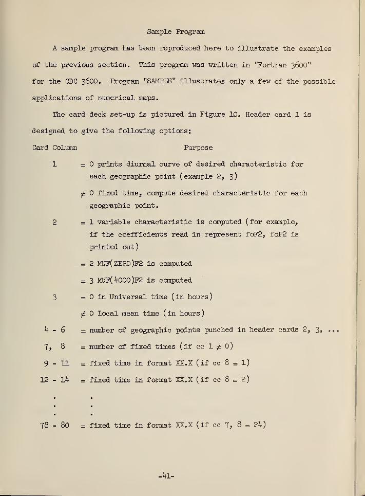
Sample Program

A sample program has been reproduced here to illustrate the examples

of the previous section. This program was written in "Fortran 3600"

for the GDC 3600. Program "SAMPLE" illustrates only a few of the possible

applications of numerical maps.

The card deck set-up is pictured in Figure 10. Header card 1 is

designed to give the following options:

Card Column Purpose

1 =0 prints diurnal curve of desired characteristic for

each geographic point ( example 2, 3

)

fi fixed time, compute desired characteristic for each

geographic point.

2 =1 variable characteristic is computed ( for example,

if the coefficients read in represent foF2, foF2 is

printed out)

= 2 MJF(ZER0)F2 is computed

= 3 MUF(^000)F2 is computed

3 = in Universal time (in hours)

^ Local mean time ( in hours

)

k - 6 = number of geographic points punched in header cards 2, 3, . .

,

J, 8 = number of fixed times (if cc 1 ^ 0)

9-11 = fixed time in format XX.X (if cc 8 = l)

12-1^ = fixed time in format XX. X (if cc 8 = 2)

78 - 80 = fixed time in format XX. X ( if cc J, 8 = 2k)

-M-

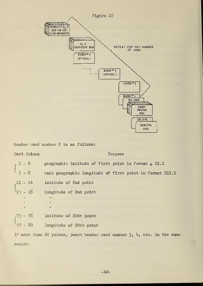
Figure 10

M(3000)F2 US,K

DECK FOR COM-

PUTING MUFW000)F2

REPEAT FOR ANY NUMBEROF JOBS

HEADER * 1

rRUN CARD

BINARY

PROGRAM

DECK

JOB CARD

SUBMITTAL

CARD

Header card number 2 is as follows:

Card Column Purpose

1 - k geographic latitude of first point in format ± XX.

X

5-8 east geographic longitude of first point in format XXX.

X

11 - Ik latitude of 2nd point

{

{15 - 18 longitude of 2nd point

73 - 76 latitude of 20th point

77 - 80 longitude of 20th point

If more than 20 points, punch header card number 3> kf etc. in the same

manner

.

-1(2-

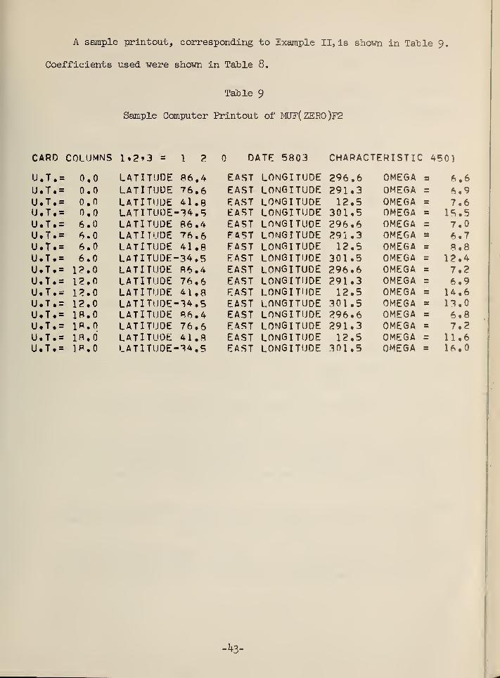
A sample printout, corresponding to Example II, is shown in Table 9,

Coefficients used were shown in Table 8.

Table 9

Sample Computer Printout of MJF( ZERO )F2

CARD COLUMNS 1«2»3 = 1 DATE 5803 CHARACTERISTIC 4501

U.T,= 0.0 LATITUDE 86,4 EAST LONGITUDE 296.6 OMEGA a 6.6U.T.= 0.0 LATITUDE 76,6 EAST LONGITUDE 291,3 OMEGA s 6.9U.T,= 0,0 LATITUDE 41.8 EAST LONGITUDE 12.5 OMEGA s 7.6U.T.= 0.0 LATITUDE-34.5 EAST LONGITUDE 301.5 OMEGA = 15.5U.T.= 6.0 LATITUDE 86,4 EAST LONGITUDE 296.6 OMEGA a 7.0U.T.= 6.0 LATITUDE 76.6 EAST LONGITUDt 291.3 OMEGA J 6.7U.T.= 6.0 LATITUDE 41.8 EAST LONGITUDE 12.5 OMEGA a 8.8U.T.= 6.0 LATITUDE--34,5 EAST LONGITUDE 301,5 OMEGA a 12.4U.T.= 12.0 LATITUDE 86.4 EAST LONGITUDE 296.6 OMEGA r 7.2U.T.= 12.0 LATITUDE 76,6 EAST LONGITUDE 291,3 OMEGA = 6.9U.T.* 12.0 LATITUDE 41,8 EAST LONGITUDE 12.5 OMEGA a 14.6U.T.= 12.0 LATITUDE-•34,5 EAST LONGITUDE 301.5 OMEGA s 13.0U.T.= 18.0 LATITUDE 86,4 EAST LONGITUDE 296.6 OMEGA s 6.8U.T.= 18.0 LATITUDE 76,6 EAST LONGITUDE 291,3 OMEGA a 7.2U.T.= 18.0 LATITUDE 41,8 EAST LONGITUDE 12.5 OMEGA a 11.6U.T.= 1B.0 LATITUDE-34.5 EAST LONGITUDE 301.5 OMEGA = 16.0

-2tf-

6. References

Appleton, E.V. (19*1-6), Nature, vol. 157, p. 691.

Bailey, D.K. (19W), Terr. Mag. and Atmos. Elect., vol jg, No. 1, 35-39-

Chapman, S. and Bartels, J., (1962), Geomagnetism, vol II, Oxford atthe Clarendon Press.

Davies, K. (1965), "Ionospheric radio Propagation," National Bureau ofStandards Monograph 80 (Chap. 7).

GHQ United States Army Forces, Office of the Chief Signal Officer,Pacific, Tokyo (May 19^6), "Report on Japanese research on radiowave propagation.

"

Haydon, G.W. and Lucas, D.L., "Theoretical considerations in the selec-tion of optimum frequencies for high frequency sky-wave communicationservices," (to he published).

Hinds, M. and Jones, W.B. (July I963), "Computer program for ionosphericmapping by numerical methods," NBS Tech. Note l8l.

ITSA Ionospheric Predictions, issued monthly 3 months in advance, U.S.Government Printing Office, Washington, D.C., 20^02.

Jensen, D.C. and Cain, J.C. (August 1962), "Interim geomagnetic field,"J. Geoph. Res., No. 9, 3568-3569.

Jones, W.B. (April 1962), "Atlas of Fourier coefficients of diurnalvariations of foF2, " NBS Tech Note 1^2.

Jones, W.B. and Gallet, R.M. (Dec. i960), "Ionospheric Mapping bynumerical methods, " ITU Telecomm. Journal No. 12, 260-26*f.

Jones, W.B. and Gallet, R.M. (May 1962a), "Representation of diurnaland geographic variations of ionospheric data by numerical methods,"ITU Telecomm. Journal 29, No. 5, 129-1*1-9; also published ( July-August 1962) Journal of Research NBS 66D (Radio Propagation),No. k, ^19-^38.

Jones, W.B. and Gallet, R.M. (Nov. -Dec. 1962b), "Methods for applyingnumerical maps of ionospheric characteristics," Journal of ResearchNBS 66D (Radio Propagation), No. 6, 6*1-9-662.

Jones, W.B. and Gallet, R.M. (Jan. 1965a), "Representation of diurnaland geographic variations of ionospheric data by numerical methods, II.

Control of instability," ITU Telecomm. Journal 32, No. 1, 18-28.

-kk-

Jones, W.B. and Gallet, R.M. (Feb. 1965b), "Atlas of Fourier coefficients

of diurnal variation of foF2. Part II. Distribution of amplitude

and phase," NBS Tech Note 305.

Lucas, D.L., Haydon, G.W., et al, "Predicting statistical performanceindexes for high frequency ionospheric telecommunication systems,"

(to be published).

-fc5-

Appendix A

Fourier Coefficients

for

foF2 Monthly Median

-hi-

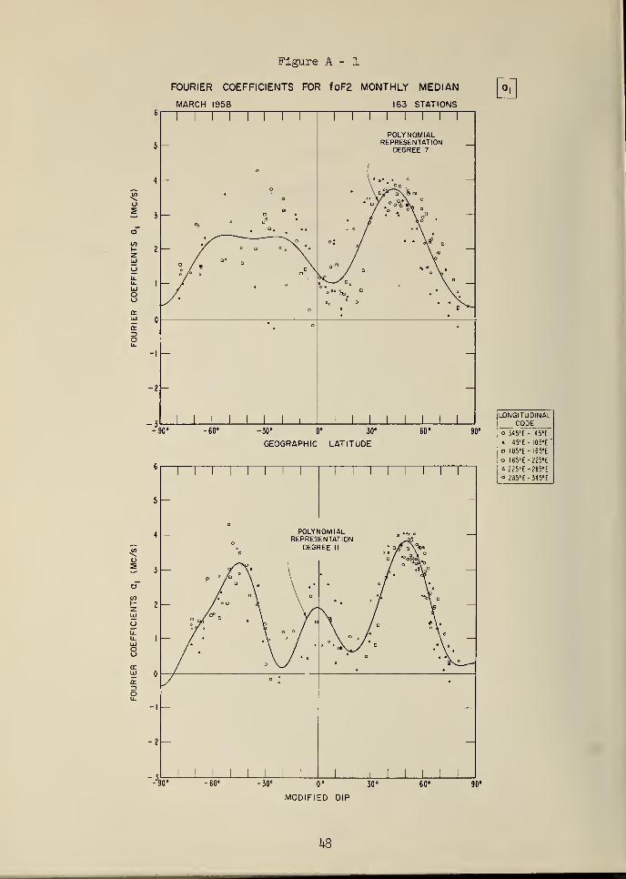
Figure A - 1

FOURIER COEFFICIENTS FOR foF2 MONTHLY MEDIAN

MARCH 1958 163 STATIONS

- J-

1 1 1 1 1 1 1 11 1 1 1 1 1

POLYNOMIAL

o

REPRESENTATION _DEGREE 7

—"

o •'

/ OV o

°*"

D

a

N. o °* /

9 *4 \ Ox ho '

a ° o \ 4

\ *\°

1 /a \ (l /•«' \ X

O /• X D N

\

«

G

xx

* °J,>^

—

1 | | 1

G

1 i 1 1 1 1 1 1 1 1

-90' -30" 0" 30* 60*

GEOGRAPHIC LATITUDE

-90 GO -30' 0° 30'

MODIFIED DIP

60°

jLONGlTUDINALCODE

,

o 345'E 45'E

« 45'E I05°E*

|

o 105-E I65'E

!o I65°E 225°E

a 225«E - 285-E

« 2B5'E -345»E

90'

k3

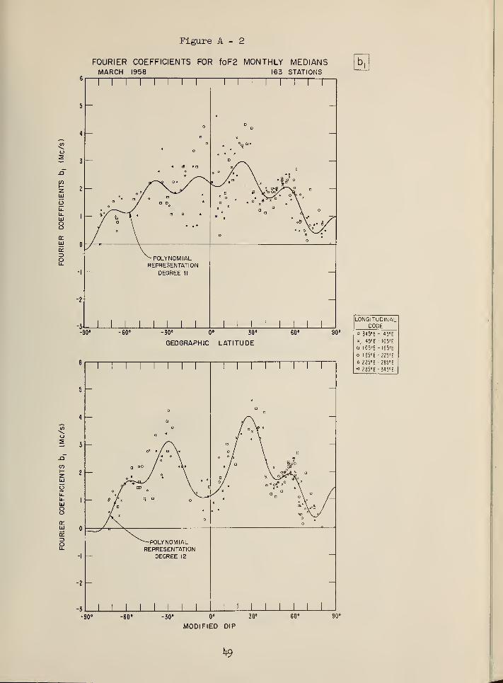
Figure A - 2

FOURIER COEFFICIENTS FOR foF2 MONTHLY MEDIANSMARCH 1958 163 STATIONS

-90"

-90°

POLYNOMIALREPRESENTATION

DEGREE 11

-60° -30° 0° 30'

GEOGRAPHIC LATITUDE

60° 90°

-POLYNOMIALREPRESENTATION

DEGREE 12

LONGITUDINALCODE

o 345°E 45°E

«. 45°E 105'E

o I05"E I65°E

o I65"E 225°E

a 225°E 285" E

« m°i 345»E

-60° -30° 0° 30°

MODIFIED DIP

60" 90°

h9

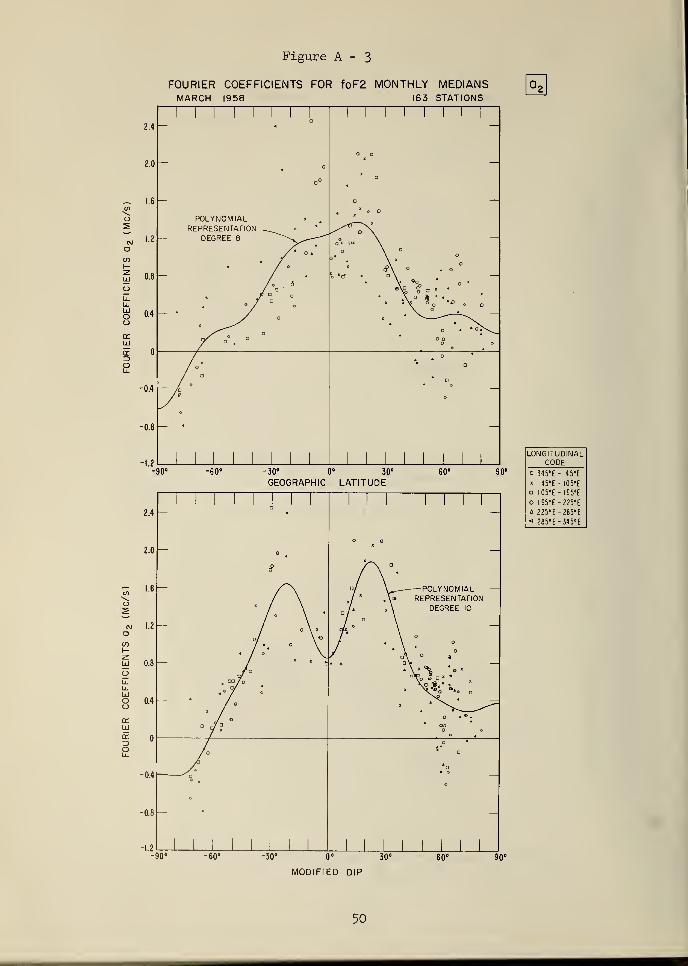
Figure A - 3

FOURIER COEFFICIENTS FOR foF2 MONTHLY MEDIANSMARCH 1958 163 STATIONS

1 1 1 1 1 1 1

ol 1 1 1 1 1 1

i

1

•IA

2.0

0°D

1.6 O —c/> x

o a

o POLYNOMIAL X*

^ REPRESENTATION _ o *

C\J1.2 DEGREE 8

o° ( , \—

o J °* o

(/)

1- < / ° « A o . o °

Ll)

Ou.u.

0.8

A a

J c

, 6

O

*o 'a 4 D \* \ °o * Q *

a\p & - x *

X ° i "

•,o

UJo 0.4 /

O\ ° 4 —

o' ^/

o ". °^\cc

*

UJ o.

I]

) » *

o / o* D

u_

/ D *

-0.4

•

-0.8

-1 ? 1 1 1 1 1 , ,

-90° -60" -30° 0" 30°

GEOGRAPHIC LATITUDE60° 90°

LONGITUDINALCODE

o 345°E m« 45°E -I05«E

o I05'E -I65*E

o I65°E -225'E

a nvi - 285-Eo 285«E •345'E

-30" 0" 30°

MODIFIED DIP

60° 90°

50

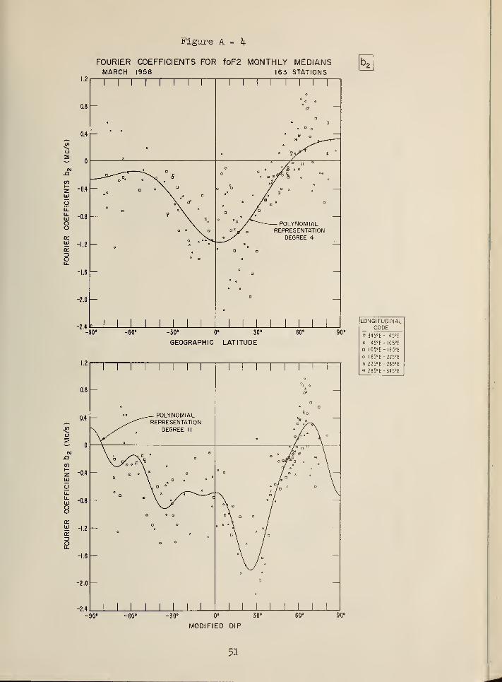
Figure A - k

FOURIER COEFFICIENTS FOR foF2 MONTHLY MEDIANSMARCH 1958 163 STATIONS

-Q

-z.

UJ

Idoo

-30" 0° 30°

GEOGRAPHIC LATITUDE

90°

LONGITUDINALCODE

o 545'E - 45'E

« 45°E I05'E

I05°E -I65°E

o I65°E -225°E

a 225°E 285'E« 2B5"E - 345-E

-30' 0° 30°

MODIFIED DIP

51

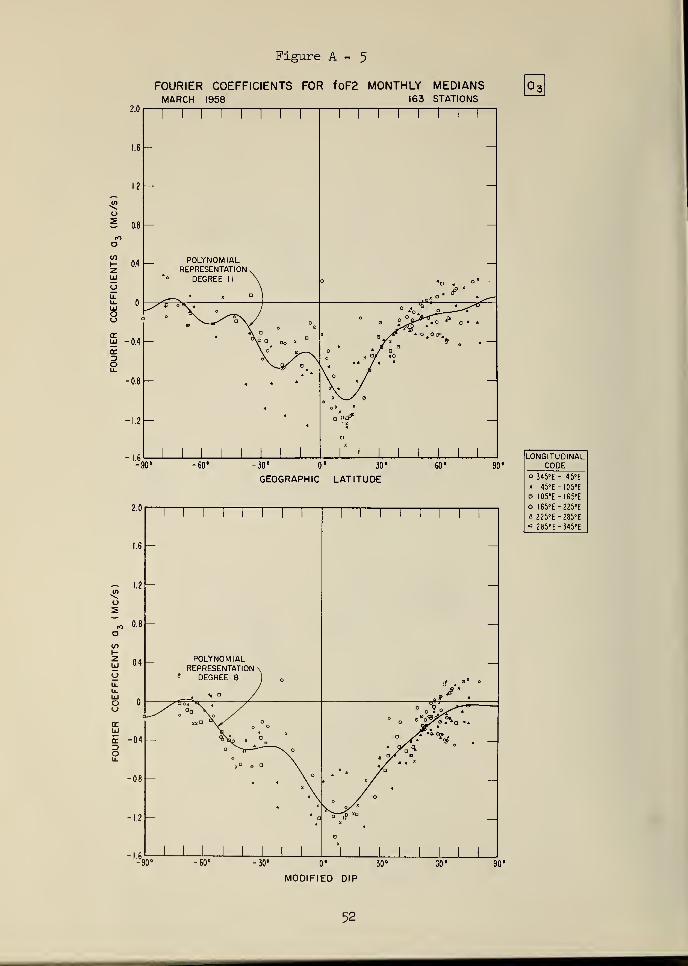
Figure A - 5

FOURIER COEFFICIENTS FOR foF2 MONTHLY MEDIANSMARCH 1958 163 STATIONS

2.0

1.6

- 1.2</>\o

to

o

0.8

0.4

-1.6

-30° 0° 30'

GEOGRAPHIC LATITUDE

POLYNOMIALREPRESENTATION

* DEGREE 8

i i—i—

r

•30° 0° 30°

MODIFIED DIP

90°

LONGITUDINALCODE

o 345°E - 45'E

x 45°E I05*E

d I05°E •I65'E

o I65°E 225'Ea ?25"E - 285°E

« 285°E -345°E

90°

52

Figure A - 6

FOURIER COEFFICIENTS FOR foF2 MONTHLY MEDIANSMARCH 1958 163 STATIONS

£ 0.

-O

CO

LL-

O

2.0

1.6-

1.2—

- 0.8

ro

CO

t 0.4

uj -0.4

o

-0.8-

-1.2-

•1.6

-60 -30" 0° 30°

GEOGRAPHIC LATITUDE

1 1 1 1 1 1 1 1

POLYNOMIAL— /-REPRESENTATION/ DEGREE II

to u

© a

a

o __ >

' "^%

u°** \ n x *y » \

o / * \

/ \ U h ° o

:i i

'

eJe." V Y

— « a

o

1

LONGITUDINALCODE

o 345-E - 45"E

« 45°E I05'Ed I05°E -I65-E

o 1 65-E •225°E

a 225-E -285°E

« ?85°E •345'E

-90° -30° 0" 30"

MODIFIED DIP

53

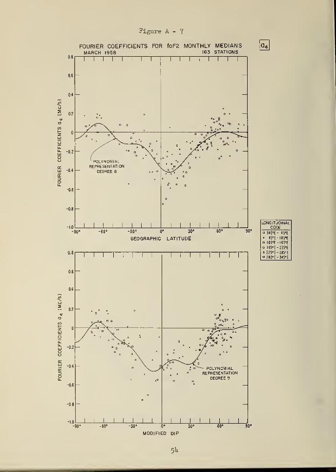
Figure A - 7

0.8

0.6

0.4

t. 0.2

UJOOa:uj -0.4

orZ>o

FOURIER COEFFICIENTS FOR foF2 MONTHLY MEDIANSMARCH 1958 163 STATIONS

t~] i i r

-0.6 —

-0.8

-1.0

-90'

0.8

0.6

0.4 _

- 0.2

oCO

£LlJ

o

-0.2

Oo

y -0.4

orz>o

-0.6 -

•0.8

-1.0

90"

POLYNOMIALREPRESENTATION

DEGREE 8

i r

o. g

*, %

¥ o

-60° -30' 0° 30" 60°

GEOGRAPHIC LATITUDE

90°

1 1 1 11 1 1 1 1 1 1 1 1 1 1 1

-

o

n^Ao " B

G *

;•„ : -

-

/ % \

o c

° oo

«

O

4 / —

-o

E" ° POLYNOMIAL

° REPRESENTATION

-

-

G

oDEGREE 9

D -

1 1 1 1 1 11 1 1

I 1 1 1 1 1

-60° -30" 0° 30°

MODIFIED DIP

60° 90'

a4

LONGITUDINALCODE

o 345°E- 45"E

* 45°E - I05*E

a 1 0S°E - I65°E

o I65°E-225»E

a 225°E-285°E< 285'E-345°E

5h

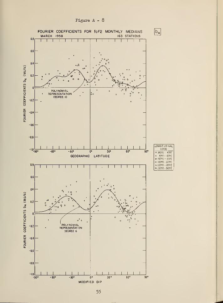
Figure A - 8

08

FOURIER COEFFICIENTS FOR foF2 MONTHLY MEDIANSMARCH 1958 163 STATIONS

0.6—

0.4

0.2-

-0.2-

UJ

oLuU.UJoo<r

y -0.4ec=>o

-0.6

-0.8

-1.0

1 1 1 1 1 1 1 1

'A aD

o a x « / o \— » ^ ~-2^/ mP \° xX „ o o Kg

/ G / V_/* D * / »

1 1 1 1 1 1 1 1

» o xX D

o ax

G —

•/ v* * •D ~

/ a * rife a " ° %D o

° PSS^ £ _ « >^"

POLYNOMIAL ,/REPRESENTATION

DEGREE 10

1 1 1 1 1 1 1 1

O X* oG * O

So . • *° °.

o

90° -60°

-90°

-30° 0° 30° 60°

GEOGRAPHIC LATITUDE

-60 -30° 0° 30'

MODIFIED DIP

60°

90°

LONGITUDINALCODE

° 345°E • 45'E

* 45°E I05"E

a 1 05°E I65*E

o I65°E 225°Ea 225-E 285'E<• 285'E 345°E

55

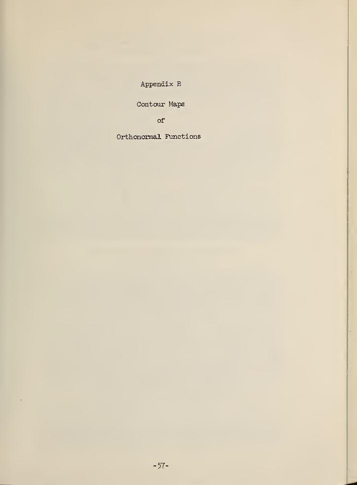
Appendix B

Contour Maps

of

Orthonormal Functions

-57-

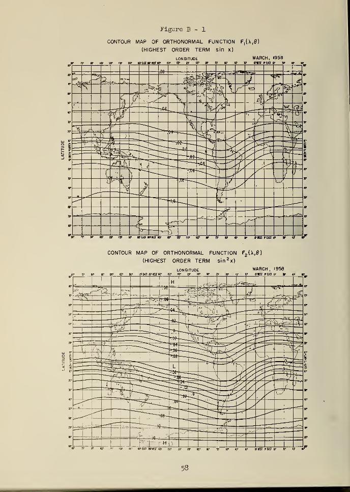
Figure B - 1

CONTOUR MAP OF ORTHONORMAL FUNCTION F,(X,0)

(HIGHEST ORDER TERM Sin x)

u »•

• ?y w w or ijt «• hjeast (piest w is- ay ar «• «• re- «• «• r is-Ka <r east » r «r

CONTOUR MAP OF ORTHONORMAL FUNCTION F2(X,0)

(HIGHEST ORDER TERM sin 2x)

SO- 75- W 105'

LONGITUDE1JS- 150- I65

-EAST ISO* WEST «• ISO* IJ5* W KB'

MARCH, 195875' to* 4V Yf 15-lfSI (T EAST 6- JO- «• »•_

»• « «• Iff 45' JT IS'IESI (PEAST IS1 Xr

58

Figure B - 2

CONTOUR MAP OF ORTHONORMAL FUNCTION F 4 (X,0)

(HIGHEST ORDER TERM sin 4 x)

LONGITUDEis

1 w ioy i»» '3y isc w east ib- iest «y w iiy gr «»• sc iy

MARCH, 1958<y »! iyitST y[Asr 6- iy «y v

60' 75' 90" IB" l»" IJ? 150- 16? EAST KTKSI 165" ISC 155" IW 105' IS' 60- «• »• 15' RSI 0-EAST IS1 nr Kf tr

CONTOUR MAP OF ORTHONORMAL FUNCTION F5 (X,0)

(HIGHEST ORDER TERM sin 5x)

LONGITUDE MARCH, 1958jr ry w my vsr >sy la1 «y east to- rer «y ar isy gr jg xr iy «r ty 30- iyitST o-east b- w ty

«• w tr or w w w «teasi wks «y isr uy w «• «r ry «r «y »• lynsr crusi v «• «r

59

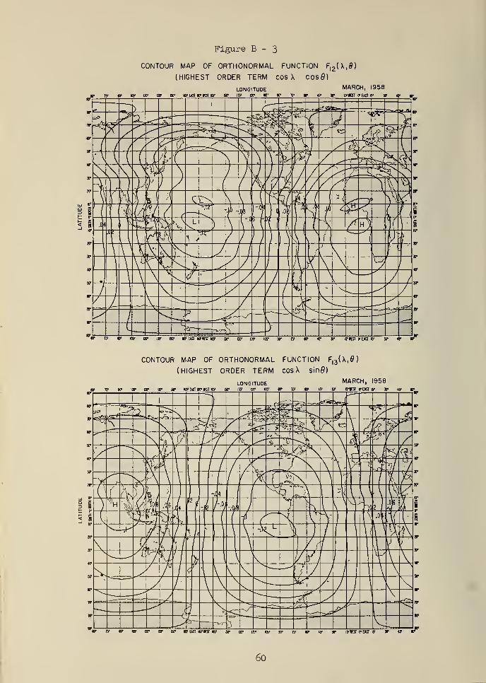
Figure B - 3

CONTOUR MAP OF ORTHONORMAL FUNCTION F|2(X,0)

(HIGHEST ORDER TERM COS X COsB)

MARCH, 1958

M I 1_«• if w w lit tiosi wrws w? «r us- iw ks* 90* is- «r «• xr lyiEST irast iy w w

CONTOUR MAP OF ORTHONORMAL FUNCTION F|3(X,0)

(HIGHEST ORDER TERM COS X sin0)

LONGITUDE MARCH.I958

«r w w wy or w isp «• ost w iet «y «r iff gr as* w ly «r «• xr lyiKt ir east y xr w p_

if tr m or i» or mua wms w ar v iir «' io- iv v w xr lyitsr ceasi ly xr w

60

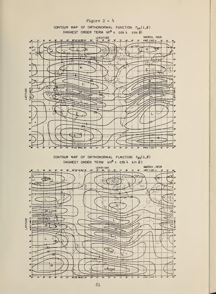
75' XT !»•

Figure B - h

CONTOUR MAP OF ORTHONORMAL FUNCTION F24 (X,0)

(HIGHEST ORDER TERM sin6 x COS X COS 6)

LONGITUDE MARCH, 1958us- iw igE*sTw»GTBy ariifBTifffii'i'ii'if lyitsi irasr y »• «• e

75' W 105- !»• IS? ISO- «? EAST KTIEST 165' ISO- 85' 130* IDS' 90' 75- »• 45' JC I5'KST 0" EAST 15* Hr «• «T

CONTOUR MAP OF ORTHONORMAL FUNCTION F25 (X,0)

(HIGHEST ORDER TERM sin6

x COS X sine)

LONGITUDEsr 75* so- ids- iw i» iso* it? east w iest is- bo1 w w kjs- so* w

MARCH , 1958«• SO" IS'lEST V EAST t,' 30- « «T

IS" »• I0S" IZ0* l» 150- S» EAST W1EST «• 1ST US' IW I0S- »• 15' «• so- lyitsi feast is- v «y

61

Appendix C

Diurnal Variation

of

Orthonormal Coefficients d.k

-63-

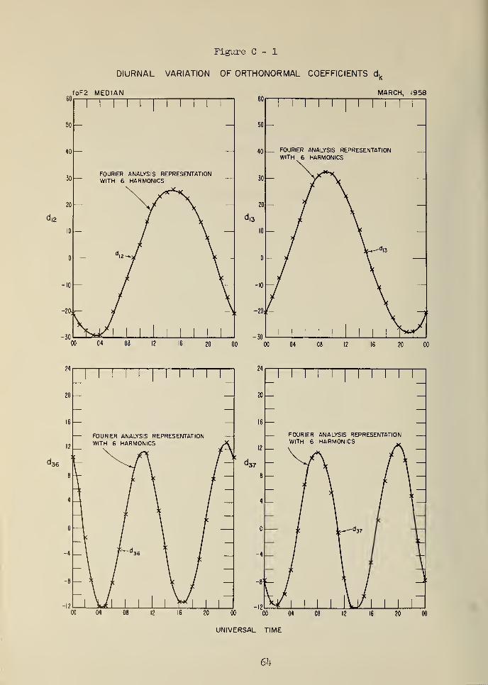
Figure C - 1

60

DIURNAL VARIATION OF ORTHONORMAL COEFFICIENTS dk

IEDIAN MARCH, 1958

40

FOURIER ANALYSIS REPRESENTATIONWITH 6 HARMONICS

60

50

40 FOURIER ANALYSIS REPRESENTATIONWITH 6 HARMONICS

20

J 36

FOURIER ANALYSIS REPRESENTATIONWITH 6 HARMONICS

00 04

24

FOURIER ANALYSIS REPRESENTATIONWITH 6 HARMONICS

20 00 00 04

UNIVERSAL TIME

6h

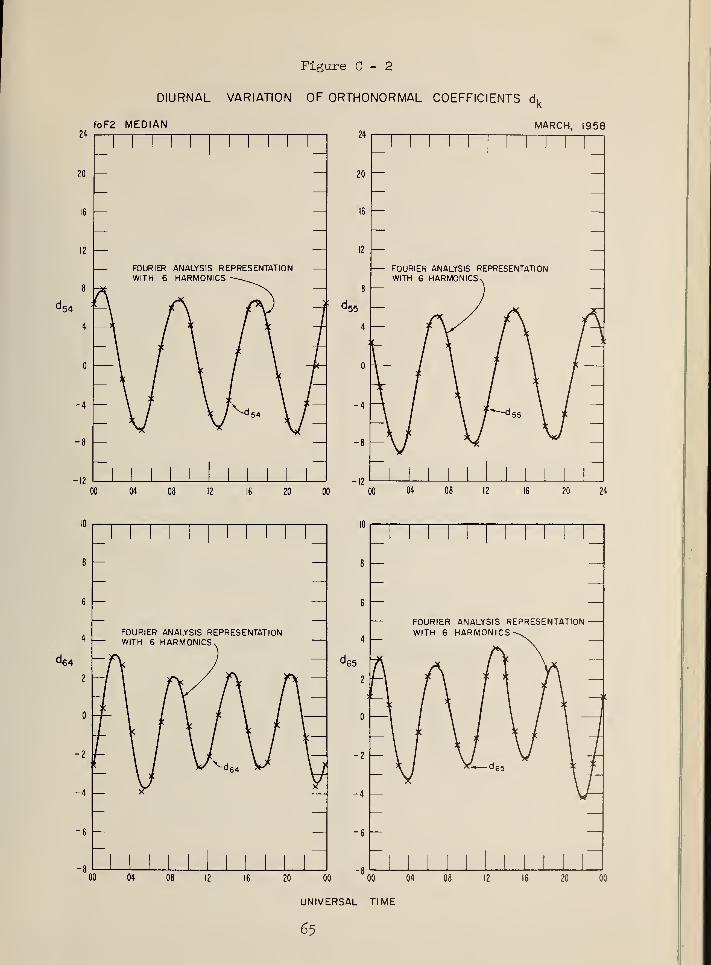
Figure C - 2

DIURNAL VARIATION OF ORTHONORMAL COEFFICIENTS dk

foF2 MEDIAN MARCH, 1958

20

—16

FOURIER ANALYSIS REPRESENTATIONWITH 6 HARMONICS

24

20

FOURIER ANALYSIS REPRESENTATIONWITH 6 HARMONICS «

20 24

^64

FOURIER ANALYSIS REPRESENTATIONWITH 6 HARMONICS,

00 04

FOURIER ANALYSIS REPRESENTATIONWITH 6 HARMONICS-

20 00 00 04

UNIVERSAL TIME

65

20 00

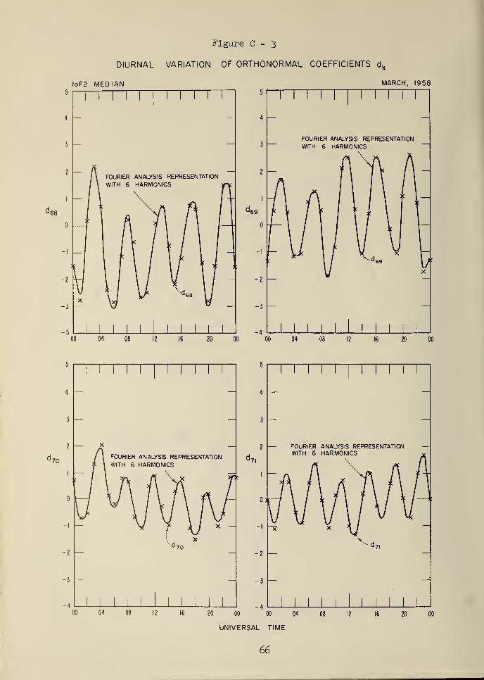
Figure C - 3

DIURNAL VARIATION OF ORTHONORMAL COEFFICIENTS dk

foF2 MEDIAN MARCH, 1958

J68

-5

00 04

4 —

FOURIER ANALYSIS REPRESENTATIONWITH 6 HARMONICS

12 16 20 04 08 12 16 20

3—

J 70

-3

FOURIER ANALYSIS REPRESENTATIONWITH 6 HARMONICS

04 08 12 16

-4

FOURIER ANALYSIS REPRESENTATIONWITH 6 HARMONICS

20 00 00 04

UNIVERSAL TIME

12 16 20 00

66

foF2 MEDIAN

Figure C - h

DIURNAL VARIATION OF ORTHONORMAL COEFFICIENTS d k

MARCH, 1958

FOURIER ANALYSIS REPRESENTATIONWITH 6 HARMONICS

3 —

4 —

FOURIER ANALYSIS REPRESENTATIONWITH 6 HARMONICS -

3 —

00 04 08 12 16 20 00 00 04 08 12 16 20 24

2.0

d™ -

FOURIER ANALYSIS REPRESENTATIONWITH 6 HARMONICS-

X

2.0

1.6 —

-FOURIER ANALYSIS REPRESENTATIONWITH 6 HARMONICS -

20 00 00

UNIVERSAL TIME

67

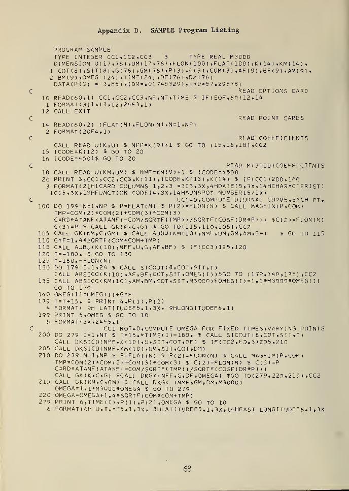
Appendix D. SAMPLE Program Listing

PROGRAM SAMPLETYPE INTEGER CC1,CC2»CC3 $ TYPE REAL M3000DIMENSION U( 17 »76) »UM( 17,76) »FLON ( 100 ) ,FLAT ( 100 ) »KL( 14 ) *KM ( 14 ) »

1 COT(8 ) »SIT( 8) ,G(76) ,GM( 76) »P(3 ) »C(3 ) ,COM< 3 ) ,AF ( 9 ) ,BF ( 9 ) , AM ( 9 )

,

2 BM(9)»OMEG ( 24) , T IME ( 24 ) ,DF ( 76 ) ,DM ( 76

)

DATA(P(3) = 3. E5 )» (DR=. 01745329) , <RD=57. 29578)READ OPTIONS CARD

10 READ(60,1) CC1 ,CC2 ,CC3 ,NP,NT,T IME $ I F ( EOF ,60 ) 12 14

1 FORMAT

(

311 ,13, 12, 24F3.1 )

12 CALL EXITREAD POINT CARDS

14 READ(60,2) ( FLAT ( N ) , FLON ( N ) , N= 1 ,NP

)

2 FORMAT ( 20F4.1 )

READ COEFFICIENTSCALL READ U(K,U) $ NFF = K(9) + 1 $ GO TO ( 1 5 , 16 , 1 8 ) ,CC2

15 ICODE=K(12) $ GO TO 2016 ICODE=4501$ GO TO 20

READ M(3000 (COEFFICIENTS18 CALL READ U(KM,UM) $ NMF=KM(9)+1 $ ICODE=450820 PRINT 3,CC1,CC2,CC3,K{ 11) ,ICODE,K( 13) ,K(14) $ IF ( CC1 ) 200 . 1"03 FORMAT

(

21H1CARD COLUMNS 1,2,3 = 3 I 3 , 3X ,4HDATE I 5 , 3X , 14HCHAR ACT ER I ST I

1CI5,3X , 13HFUNCTION CODE I 4 , 3X , 14HSUNSP0T NUMBERI5/1X)CC1=0, COMPUTE DIURNAL CURVE, EACH PT

.

100 DO 199 N=1,NP $ P=FLAT(N) $ P(2)=FL0N(N) £ CALL MAGFI N ( P ,C0M

)

TMP=COM( 2 )*COM(2 ) +COM ( 3 ) *COM ( 3

)

C=RD*ATANF(ATANF< -COM/SQRTF( TMP ) ) /SQRTF ( COSF ( DR*P ) ) ) SC ( 2 )=FLON(N

)

C(3)=P $ CALL GK(K,C,G) J GO TO ( 1 1 5 , 1 1 , 1 05 ) ,CC2105 CALL GK(KM,C,GM) J CALL A J3 J ( KM ( 1 ) ,NMF , UM ,GM , AM , 6M ) $ GO TO 115110 GYF=1.4*SQRTF ( COM*COM+TMP

)

115 CALL AJBJ(K( 10) ,NFF,U,G,AF,BF) $ I F ( CC3 ) 12 5 , 1 2

120 T=-180. $ GO TO 130125 T=180.-FLON( N)130 DO 179 1 = 1,24 $ CALL S I COJT ( 8 ,COT , S I T , T )

CALL ABSICCf K( 10 ) ,AF,BP,COT,SIT,OMEG( I ) ) JGO tq ( 1 79 , ] 40 , 1 35 ) ,CC2135 CALL ABSICCI KM ( 10 ) , AM ,BM , COT ,S I T ,M300 ) SOMEG ( I ) =1 . 1*M3000*OMEG I I

)

GO TO 179140 OMEGt I ) =OMEG( I )+GYF179 T=T+15. S PRINT 4,P(1),P(2)

4 FORMAT ( 9H LAT I TUDEF5 . 1 , 3X , 9HLONG I TUDEF6 . 1

)

199 PRINT 5,OMEG S GO TO 105 FORMAT ( 3X,24F5.1 )

CC1 NOT = 0, COMPUTE OMEGA FOR FIXED T

I

MES , VARY I NG POINTS200 DO 279 1=1, NT $ T = 15 .*T IME ( I )- 180 . $ CALL S I COJT ( 8 ,COT , 8 I T , T

)

CALL DKSICO( NFF,K ( 10) ,U, SIT, GOT ,DF ) S I F ( CC2 . EQ . 3 ) 20 5 , 2 1

205 CALL DKSICOt NMF,KM( 10) ,UM,SIT ,COT ,DM)210 DO 279 N=1,NP $ P = FLAT(N) $ P(2)=FLON{N) $ CALL MAGF I N ( P , COM )

TMP=COM(2)*COM(2 )+COM( 3 )*COM(3 ) £ C(2)=FLON(N) $ C(3)=PC=RD*ATANF ( ATANF ( -COM /SQRT P

( TMP) ) /SQRTF (COSF ( DR*P ) ) )

CALL GK(K,C,G) $CALL DKGK ( NFF , G , DF ,OM EGA ) $GO TO ( 2 79 , 220 , 2 1 5 ) , CC2215 CALL GK(KM,C,GM) $ CALL DKGK ( NMF , GM , DM , M3000

)

OMEGA=l. l*M3U00*OMEGA $ GO TO 27922 OMEGA=OMEGA+ 1.4* SQRTF (COM*COM+TMP

)

279 PRINT 6, TIME ( I ) ,P( 1 ) ,P(2) , OMEGA $ GO TO 106 FORMAT(6H U . T . = F5 . 1 , 3x , 8HLA T I TUOE F5 . 1 , 3X , 14HE AST LONG I TUDEF6 . 1 , 3X

68

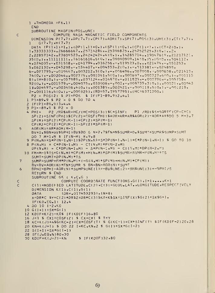
1 ,7H0MEGA =F6.1)ENDSUBROUTINE MAGFI N ( POS »UNE

)

C COMPUTE NASA MAGNETIC FIELD COMPONENTSDIMENSION P(7,7),DP(7,7),CP<7) , AOR ( 7) ,SP (7 ) ,POS( 3 ) ,UNE ( 3 ) ,CT ( 7 , 7 ) ,

1 G(7*7) *H( 7,7)DATA (P(1»1)=1.),(DP(1,1)=0.),(SP(1)=0.),(CP(1)=].),(CT=2(0.)»1.33333 333 » .26666667 , .2 5714286,. 25396825 , • 25252 525 ,3 ( 0. ) ». 2,2. 22857 142 *• 2 3809523,. 24242424,4 ( 0. ) ,.14285 714,. 190476 19,. 212 12121,35(0.) ,.11111111,. 16161616, 6(0.) , . 09090909 , 14 ( . )'),( G=0. » .304112 ,

4.024035,-.031518,-.041794,.016256,-.019523,0.,.02 1474,-.0512 53

,

5. 062 13 0, -.04 52 98, -.0 3440 7, -.004 3 5 3, 2 (0.),-. 013381, -.024898,6-. 02 17 95, -.019447, .00 3212, 3(0.) ,-.006496,. 00 7 00 8, -.0006 8 ,.021413

,

74(0.), -.00 2044, .002 775,. 00 1051, 5(0.), . 00069 7 ,. 000227 , 6 ' . ) -.0011158), (H = 8(0.),-. 057989, .033 124, .01 4870, -.011825, -.000796, -.005758,92(0. )

,-.0015 79,-.OO4O7 5,.010OO6,-.O02,-.OO873 5,3(0. ) , .0002 1 , . 00O431 J.00459 7,-.003406,4(0. ) , . 001385 ,. 00242 1 ,-.000113 ,5(0.!, -.00 1213,2-. 001116, 6(0.) ,-.0003 2 5 ),(RD= 57. 2957795), (HC =6371200.)P2 = POS(2) $ Pl=POS $ IF(P1-89.9)2,4,1

1 Pl=89.9 $ P2 = $ GO TO 4

2 IF(Pl+89.9)3,4,43 Pl=-89.9 $ P2 =

4 PHI= P2 /RD$AR=HC/ (HC+POS( 3 ) )$C=SINF( PI /RD) $S=SQRTF (CP-C*C

)

SP(2)=SINF(PHI)SCP(2 )=COSF(PHI ) $AOR=AR*ARSAOR ( 2 )=AOR*AR$DO 5 M=3,7SP(M)=SP(2 )*CP(M-1 )+CP(2)*SP(M-l)CP(MJ=CP(2)*CP(M-1)-SP(2 )*SP(M-1)

5 AOR (M)=AR*AOR(M-l )

BV=0.$BN=bV$bPHI =8v$DO 6 N = 2 ,7$FN=NSSUMR=0. $SUMT = S'JMR$SUMP=SUMTDO 7 M=l ,N $ IF(N-M) 8,9,8

9 P(N,N) =S*P(N-1 ,N-1 )$DP (N,N) =S*DP ( N- 1 ,N-1 )+C*P( N-l ,N-1 ) $ GO TO 10

8 P(N,M) = C*P(N-1,M) - CT (N»M)*P(N-2 ,M

)

DP(N,M) = C*DP(N-1,M) - S*P<N-1,M) - CT ( N ,M ) *DP ( N-2 ,M

)

10 FM =M-1STS = G( N,M> *CP(M) +H( N,M)*SP(M) $SUMR =SUMR+P ( N ,M) *TSSUMT=SUMT+DP(N,M) *TS

7 SUMP=SUMP+FM*P(N,M)* ( -G ( N ,M ) *SP ( M ) +H ( N ,M ) *CP ( M )

)

BV=BV+AOR(N) *FN*SUMR $ BN=BN-A0R ( N ) *SU^T6 BPHI=BPHI-AOR(N)*SUMPSijNE ( 1 ) =-BV$UNE ( 2 )=BN$ljNE (3)=-BPHI /S

RETURN $ ENDSUBROUTINE GK ( K,C,G )

C COMPUTE COORDINATE FUNCT IONS ,G ( I ) , 1=1 »• . • »K+1C C(

1

)=MODIFItD LATITUDE. C( 2>» C(3)=GEOG. LA T. , LONG I TUDE , RESPEC TI VELY

DIMENSION <( 1) ,C( 1) ,G(1

)

DATA (DR=. 017453293) , (N=8)X=DR*C $Y=C( 2)*DR$Z=DR*C(3)4K0=K$SX=SINF(X)SG(2)=SXSG=1.IF(KO.EQ.l) 12,4

4 DO 10 1=2, KO10 G( I+1)=SX*G( I

)

12 KDIF=K(2)-K0S I F ( KDI F ) 16 , 8016 J=l $ CX1=C0SF(Z) $ CX=CX1 $ T=Y18 KC=K< J)+4$G(KC-2 )=CX*COSF(T) $ G ( K.C-1 ) =CX*SI NF ( T ) $ I F ( KD I F-2 ) 20 , 28

20 KN=K(J+1) $ DO 22 I=KC,KN,2 $ G { I) =SX*G ( 1-2

)

22 G( I+1)=SX*G( 1-1)28 IF( J.EQ.N)80,3030 KDIF=K( J+2 )-<N S I F

(

KDI F ) 32 , 80

69

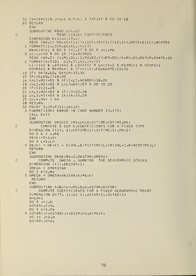
32 CX=CX*CX1$ J = J+1 $ FJ=J 1 T=FJ*Y $ GO TO 18

80 RETURNENDSUBROUTINE READ U(K.U)

READ U(S»K) COEFFICIENTSDIMENSION K( 1 ) ,U( 17,1

)

READ (60,1) KD, (K( I ) , I =1 , 10) , <K( I ) , 1 = 12 ,14 ) ,DATA,K ( 11 ) ,NCARDS1 FORMATt II ,13I5,6X,A1 ,14, 13)MX=K(9)+1 $ DO 5 1=1,17 f DO 5 J=l ,MX

5 U(I,J)=0 $ DO 25 I=1,NCARDSREAD (60,2) II, Ml ,D1 , I2,M2,D2, I3,M3,D3, I 4, M4 , D4 , DATUM , KDATE , ID

2 FORMAT (4(2 12, E 14. 7 ) , Al , 14 , I 3

)

L1=I1+1 $ L2=I2+1 $ L3=I3+I $ L4=I4+1 $ M1=M1+1 $ M2=M2+1M3=M3+1 $ M4=M4+1 S I F ( K ( 1 1 ) . EQ.KDA TE ) 1 , 30

10 IF( DATA.EQ. DATUM)15,3015 IF( ID.EQ.I ) 16,3016 U(L1,M1)=D1 5 IF( I .LT.NCARDS) 18,2018 U(L2,M2)=D2 J U(L3,M3)=D3 $ GO TO 2520 IF( 12)21,2821 U(L2,M2)=D2 $ IF(I3)22,2822 U(L3,M3)=D3 S IF(I4)25,2825 U(L4,M4) = D428 RETURN30 PRINT 3,ID,K( 11 ) ,K( 12

)

3 F0RMAT(23H1 ERROR IN CARD NUMBER 13,215)CALL EXITENDSUBROUTINE DKSICO ( MX ,LH , D ,S I T I ME ,COT I ME ,DK

)

COMPUTE D SUB K ,COEFF I C I ENTS FOR A FIXED TIMEDIMENSION D(17, 1 ) ,COT I ME ( 1 ) ,S I T I ME ( 1 ) ,DK ( 1

)

DO 5 K = 1 ,MXDK(K )=D( 1 ,K)DO 5 L=1,LH

5 DK(K) = DK(K) + D ( 2*L , K ) * S I T I ME ( L ) +D ( 2*L + 1 , K ) *COT I ME ( L

)

RETURNENDSUBROUTINE DKGK ( MX ,G ,DKST AR , OMEGA

)

COMPUTE OMEGA , SUMMING THE GEOGRAPHIC SERIESDIMENSION G( 1 ) ,DKSTAR( 1

)

OMEGA = G*DKSTARDO 5 K=2,MX

5 OMEGA = OMEGA+DKSTAR(K)*G(K)RETURN

ENDSUBROUTINE A JBJ ( LH ,MX D ,G , AS TAR ,BSTAR

)

COMPUTE COEFFICIENTS FOR A FIXED GEOGRAPHIC POINTDIMENSION D(17, 1),G( 1 ) , ASTAR ( 1 ) , BSTAR ( 1

)

N=LH+1DO 5 J=1,NASTARt J) =0.DO 5 K=1,MX

5 ASTAR(J)=ASTAR(J)+D(2*J-1,K)*G(<)DO 10 J=2,NBSTAR( J)=0.

TO

DO 10 K=1,MX10 BSTAR(J)=BSTAR(J)+D(2*J-2»K)*G(K)

RETURNENDSUBROUTINE ABSI CO ( LH , AST AR ,BSTAR , COT I ME , S I T I ME , CM EGA

)

COMPUTE OMEGA , SUMMING THE FOURIER SERIESDIMENSION C0TIME(1),SITIME(1),ASTAR(1),BSTAR(1)OMEGA=ASTARDO 5 J=1,LH

5 OMEGA =OMEGA+ AST AR ( J+l

)

*COTIME ( J ) +BSTAR ( J+l ) *SI TIMEf J

)

RETURNENDSUBROUTINE S I COJT ( L ,C , S * A )

COMPUTE SIN( JT) ,COS( JT) »J=1»... »LDIMENSION C( 1 ) ,S ( 1

)

T=.01745329*A $ C = COSF ( T ) S S = SINF(T)C( I )=C*C( 1-1 )-S*S( 1-1

)

10 S( I )=C*S( 1-1 )+S*C( 1-1 ) i RETURNEND

FOR ANGLE A

$ DO 10 1=2,

L

71 GPO 857-880

U.S. DEPARTMENT OF COMMERCEWASHINGTON, D.C. 20230

OFFICIAL BUSINESS

POSTAGE AND FEES PAID

U.S. DEPARTMENT OF COMMERC

TECHNICAL NOTE no. 338 - NOT ISSUED