Jyotish: Constructive approach for context predictions of ...

Pervasive and Mobile Computing ( ) –

Contents lists available at SciVerse ScienceDirect

Pervasive and Mobile Computing

journal homepage: www.elsevier.com/locate/pmc

Jyotish: Constructive approach for context predictions of peoplemovement from joint Wifi/Bluetooth traceLong Vu ∗, Quang Do, Klara NahrstedtDepartment of Computer Science, University of Illinois, IL61801, USA

a r t i c l e i n f o

Article history:Available online xxxx

Keywords:People movement predictionPeople movement traceWifi traceBluetooth trace

a b s t r a c t

It is well known that people movement exhibits a high degree of repetition since peoplevisit regular places andmake regular contacts for their daily activities. This paper1 presentsa novel framework named Jyotish,2 which constructs a predictive model by exploiting theregularity of peoplemovement found in the real jointWifi/Bluetooth trace. The constructedmodel is able to answer three fundamental questions: (1) where the person will stay,(2) how long she will stay at the location, and (3) who she will meet.

In order to construct the predictive model, Jyotish includes an efficient clusteringalgorithm to clusterWifi access point information in theWifi trace into locations. Then, weconstruct a Naive Bayesian classifier to assign these locations to records in the Bluetoothtrace and obtain a fine granularity of people movement. Next, the fine grain movementtrace is used to construct the predictive model including location predictor, stay durationpredictor, and contact predictor to provide answers for three questions above. Finally, weevaluate the constructed predictive model over the real Wifi/Bluetooth trace collected by50 participants in University of Illinois campus from March to August 2010. Evaluationresults show that Jyotish successfully constructs a predictive model, which provides aconsiderably high prediction accuracy of people movement.

© 2011 Elsevier B.V. All rights reserved.

1. Introduction

The ability to accurately predict people movement is crucial to numerous domains such as wireless networks, HCI, socialscience, urban planning, transportation, etc. While predicting the movement of a person, we seek the answers to threefundamental questions: (1) where will the person stay at a future time (i.e., location)? (2) how long will she stay at thelocation (i.e., stay duration)? and (3) who will she meet (i.e., contact)? Providing answers to the three questions altogetherremains challenging due to the: (1) complex nature of people movement, and (2) lack of a realistic people movement traceused to construct an accurate predictive model of people movement. On the other hand, it has been shown that peoplemovement exhibits a high degree of repetition, in which people visit regular places for their daily activities [1]. As a result,there have been previous projects that exploited the regularity in past movement to predict future movement of people.

The first class of prediction methods focused on predicting location of people movement [2–5], which essentially onlyanswered the first question above regarding the future location of people. In particular, a large number of previous papersused the association trace between the laptop/PDA and the Wifi access points (i.e., WLAN trace) to derive and evaluatetheir location predictors [4,3]. However, there was a fundamental weakness of using WLAN trace [6–10] in constructinglocation predictor since the laptop user did not always turn on the laptop and did not always carry it with her. So, the

∗ Corresponding author.E-mail addresses: [email protected], [email protected] (L. Vu), [email protected] (Q. Do), [email protected] (K. Nahrstedt).

1 This work is supported by Boeing Trusted Software Center at the Information Trust Institute, University of Illinois.2 In Sanskrit, Jyotish (Ji-o-tish) is the person who predicts future events.

1574-1192/$ – see front matter© 2011 Elsevier B.V. All rights reserved.doi:10.1016/j.pmcj.2011.07.004

http://dx.doi.org/10.1016/j.pmcj.2011.07.004

http://www.elsevier.com/locate/pmc

http://www.elsevier.com/locate/pmc

mailto:[email protected]




http://dx.doi.org/10.1016/j.pmcj.2011.07.004

2 L. Vu et al. / Pervasive and Mobile Computing ( ) –

collected associations of laptops and theWifi access points could be potentially used to understand thewireless usage ratherthan to accurately predict the location of people. Other previous projects used cellular data trace to construct the locationpredictor [11,12], in which the location was inferred from the cellular base station. However, since the transmission rangeof the cellular base station was ranging from several hundred meters (e.g., 500 m) to kilometers (e.g., 30 km), the locationpredictor derived by this inferred location might not provide needed fine granularity and accuracy.

The second class of prediction methods answered the first two questions by providing predictions for the stayduration [13] or location and stay duration [8,14]. McNamara et al. predicted the stay duration of commuters of the subwaysto select the best source of media content [13]. Lee and Hou modeled user mobility by a semi-Markov process and deviseda timed location prediction algorithm that predicted the future access point (i.e., the location in the paper’s context) of theuser and the association duration [8]. Since the model was constructed and evaluated by the WLAN trace, it suffered fromthe same fundamental weaknesses as discussed in the previous paragraph.

Recently, there have been several projects collecting ad hoc contact traces using portable experiment devices such asiMote, cellphone and PDA [15–19]. These traces can be used to answer the third question about future contact. However,these traces did not have the location information and thus could not be used to answer the first two questions.

We recently deployed the UIM scanning system on Google Android phones (i.e., UIM stands for University of IllinoisMovement) to collect MAC addresses of Wifi access points and Bluetooth devices in the proximity of the experimentparticipants [20,21]. We observe that Wifi access point information can be used to infer location [22] while Bluetooth MACscan be used to infer contact [15,16]. The joint Wifi/Bluetooth trace thus can be used to study people movement. This paperpresents the Jyotish framework, which exploits the regularity of people movement found in the joint Wifi/Bluetooth tracecollected by the UIM system to construct a predictive model of people movement. In summary, our paper has the followingcontributions:

1. To the best of our knowledge, Jyotish is the first framework, which constructs a predictive model of people movementfrom the joint Wifi/Bluetooth trace.

2. Also, to the best of our knowledge, the constructed predictive model is the first to predict future location, stay durationat the location, and contact all together.

3. We present an efficient clustering algorithm to cluster Wifi access point information into locations by exploiting theregularity of people movement. Our algorithm overcomes the Wifi signal fluctuation in previous work [23,24] andprovides a finer grain of location than that derived from cellular base station [12].

4. We evaluate the constructed predictive model over the Wifi/Bluetooth trace collected by 50 experiment participants inUniversity of Illinois campus from March to August 2010.

This paper is organized as follows. We present the trace collected by the UIM system and an overview of the Jyotishframework in Section 2. Then, we present a clustering algorithm to cluster Wifi access point information into locations inSection 3. These locations will be assigned to records in the Bluetooth trace in Section 4. Then, the Bluetooth trace withassigned location will be used to construct the predictive model in Section 5. Finally, we evaluate the predictive model inSection 6 and conclude the paper in Section 7.

2. Overview of UIM trace and Jyotish

2.1. UIM collected trace

We deployed the UIM scanning system [20] on Google phones carried by 123 participants fromMarch to August 2010 atthe University of Illinois campus, with three rounds: from the beginning of March to the end of March, from the beginningof April to the mid of May, and from the end of May to the mid of August. Table 1 shows the overall statistics of the collectedtrace.Many participantswere involved fromonemonth to twomonths of experiment.More details of theUIM systemand itscollected data set can be found in our previous paper [20]. Note that in Section 6, we evaluate Jyotish over theWifi/Bluetoothtraces collected by 50 participants in the set of 123 participants.

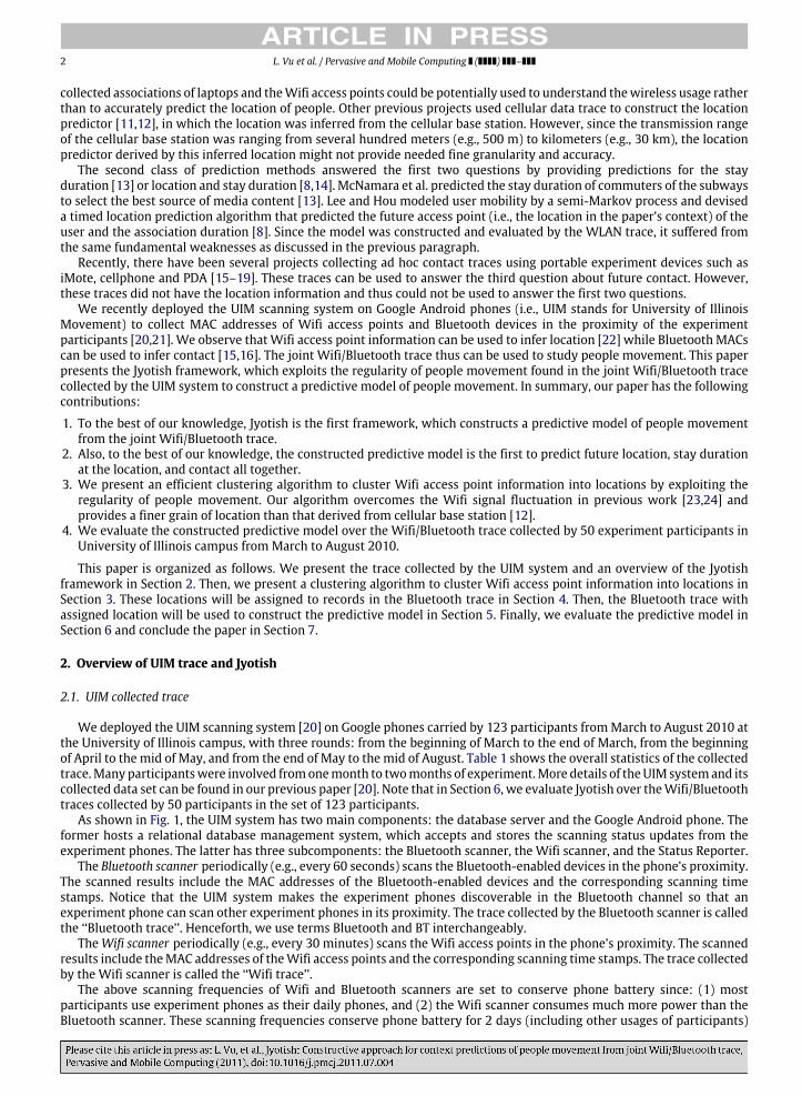
As shown in Fig. 1, the UIM system has two main components: the database server and the Google Android phone. Theformer hosts a relational database management system, which accepts and stores the scanning status updates from theexperiment phones. The latter has three subcomponents: the Bluetooth scanner, the Wifi scanner, and the Status Reporter.

The Bluetooth scanner periodically (e.g., every 60 seconds) scans the Bluetooth-enabled devices in the phone’s proximity.The scanned results include the MAC addresses of the Bluetooth-enabled devices and the corresponding scanning timestamps. Notice that the UIM system makes the experiment phones discoverable in the Bluetooth channel so that anexperiment phone can scan other experiment phones in its proximity. The trace collected by the Bluetooth scanner is calledthe ‘‘Bluetooth trace’’. Henceforth, we use terms Bluetooth and BT interchangeably.

TheWifi scanner periodically (e.g., every 30 minutes) scans the Wifi access points in the phone’s proximity. The scannedresults include theMAC addresses of theWifi access points and the corresponding scanning time stamps. The trace collectedby the Wifi scanner is called the ‘‘Wifi trace’’.

The above scanning frequencies of Wifi and Bluetooth scanners are set to conserve phone battery since: (1) mostparticipants use experiment phones as their daily phones, and (2) the Wifi scanner consumes much more power than theBluetooth scanner. These scanning frequencies conserve phone battery for 2 days (including other usages of participants)

L. Vu et al. / Pervasive and Mobile Computing ( ) – 3

Table 1Overall characteristics of UIM collected trace.

Overall characteristics

Number of participants 28 79 16Experiment period 03/01–03/20 04/08–05/15 05/24–08/16Number of days 19 38 85BT scanning period (sec, δB) 60 60 60Wifi scanning period (min, δW ) 30 20 30Number of scanned BT MACs 8508 17080 7360Number of scanned Wifi AP MACs 7004 29324 6822

Participant information

Number of CS faculties 2 2 0Number of CS staff 1 1 0Number of CS grads 14 30 12Number of CS undergrads 8 43 1Number of ECE grads 2 2 2Number of ABE grad 1 1 1

Fig. 1. UIM system architecture.

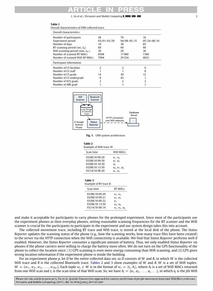
Table 2Example of Wifi traceW .

Scan time Wifi MACs

03/08/10 09:20 a1, a303/08/10 09:50 a1, a503/08/10 10:20 a603/08/10 13:50 a4, a7, a903/14/10 08:20 a1, a3

Table 3Example of BT trace B.

Scan time BT MACs

03/08/10 09:20 u1, u303/08/10 09:21 u1, u303/08/10 09:22 u103/08/10 13:50 u4, u903/14/10 08:14 u1, u3, u8

and make it acceptable for participants to carry phones for the prolonged experiment. Since most of the participants usethe experiment phones as their everyday phones, setting reasonable scanning frequencies for the BT scanner and the Wifiscanner is crucial for the participants to participate in the experiment and our system design takes this into account.

The collected movement trace, including BT trace and Wifi trace, is stored at the local disk of the phone. The StatusReporter updates the scanning status of the phone (e.g., how the scanning works, how many trace files have been created)to the server via the HTTP connection when the Wifi connectivity is available. We find that Status Reporter performs well ifenabled. However, the Status Reporter consumes a significant amount of battery. Thus, we only enabled Status Reporter onphones if the phone carriers were willing to charge the battery more often. We do not turn on the GPS functionality of thephone to collect the location since: (1) GPS scanning is even more energy consuming than Wifi scanning, and (2) GPS giveswrong location information if the experiment phone is inside the building.

For an experiment phone p, let D be the entire collected data set, so D consists of W and B, in which W is the collectedWifi trace and B is the collected Bluetooth trace. Tables 2 and 3 show examples of W and B. W is a set of Wifi tuples:W = w1, w2, w3, . . . , w|W |. Each tuple wi ∈ W is in the format of wi = ⟨ti, Ai⟩, where Ai is a set of Wifi MACs returnedfrom one Wifi scan and ti is the scan time of that Wifi scan. So, we have Ai = a1, a2, . . . , aj, . . ., in which aj is the jth Wifi


Fig. 2. Overview of Jyotish framework.

MAC scanned by the Wifi scanner of p during the entire experiment period. In Table 2, each row is one tuple wi. Let WA bethe set of all Wifi MACs scanned by theWifi scanner for the entire experiment period of one experiment phone. For Table 2,WA = a1, a3, a4, a5, a6, a7, a9.

Similarly, B is a set ofmultiple BT tuples: B = b1, b2, b3, . . . , b|B|. Each tuple bi ∈ B is in the format of bi = ⟨ti,Ui⟩, whereUi is a set of BTMACs returned fromoneBT scan and ti is the scan timeof that BT scan. So,wehaveUi = u1, u2, . . . , uj, . . ., inwhich uj is the jth BTMAC scanned by the BT scanner of p during the entire experiment period. Let BA be the set of all BTMACsscanned by the BT scanner for the entire experiment period of one experiment phone. For Table 3, BA = u1, u3, u4, u8, u9.Notice that since the Wifi scanner and the BT scanner run concurrently, the scan times of tuples of W and B overlap. Thisinformation is used in Section 4 to assign location to BT records.

Since the collected data set is in the tabular format, in this paper, we use the terms ‘‘table’’ and ‘‘set interchangeably,record’’ and ‘‘tuple’’ interchangeably. Also, we use the terms ‘‘person’’ and ‘‘phone’’, ‘‘stay duration’’ and ‘‘duration’’interchangeably.

2.1.1. Contact definitionWe say the experiment phone p has a contact with a device q whose BT MAC is uj if uj appears in one tuple of p’s BT trace B.

This contact definition can also be found in previous papers [15,16]. We assume that when p and q have a contact, the userof p and the user of q have a social contact. Henceforth, we use the term ‘‘social contact’’ and ‘‘contact’’ interchangeably.

2.2. Jyotish overview

Fig. 2 shows steps of the Jyotish framework to construct the predictive model from the joint Wifi/Bluetooth trace D. Inthe first and the second steps, we clusterWifi records inW into locations (see Section 3). Then, in steps 3 and 4, we constructa Naive Bayesian classifier to assign locations for records in BT trace B (see Section 4). In steps 5 and 6, the BT trace withassigned location is used as the input to construct location predictor, stay duration predictor, and contact predictor (seeSection 5).

3. Clustering Wifi records into locations

This section presents an algorithm called ‘‘UIM Clustering’’ to cluster Wifi records into clusters, which are used torepresent locations. This section focuses on steps 1 and 2 in Fig. 2.

3.1. UIM Clustering algorithm overview

There are several challenges in obtaining locations fromWifi records ofW . First, since theWifi signal fluctuates, althoughthe phone stays in one fixed position, it may obtain different results for different Wifi scans. Previous work [23,24] used thesignal strength to cluster Wifi MACs into locations and suffered from Wifi signal fluctuation. Second, if the phone is in themiddle of two adjacent buildings, the Wifi scanned result might be partially overlapped with the scanned results obtainedwhen the phone stays inside either of the buildings. Fortunately, the movement pattern of people is relatively regular sincethey tend to stay more frequently at their regular places. So, if two Wifi MACs a1, a3 coexist more frequently than twoWifiMACs a1, a5 in the records of Wifi trace W , then it is likely that a1, a3 stay close in a physical building. That means, it isbetter to group a1 and a3 into the same location than a1 and a5. So, we exploit the regularity of people movement to cluster


Step 1 Step 2 Step 3 Step 4

θc F

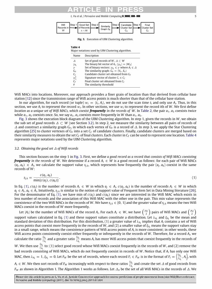
Fig. 3. Execution of UIM Clustering algorithm.

Table 4Major notations used by UIM Clustering algorithm.

Name Description

∆ Set of good records ofW , ∆ ⊂ WγAi The binary bit vector of Ai, |γAi | = |WA|

γ Set of binary vectors: γAi ∈ γ where Ai ∈ ∆

Gθ The similarity graph: Gθ = ⟨Vθ , Eθ ⟩

CC Candidate cluster set obtained from Gθ

γ SCi

Signature vector of cluster Ci ∈ CC

CF Final cluster set obtained from CCθ The similarity threshold

Wifi MACs into locations. Moreover, our approach provides a finer grain of location than that derived from cellular basestation [12] since the transmission range of Wifi access points is much shorter than that of the cellular base station.

In our algorithm, for each record (or tuple) wi = ⟨ti, Ai⟩, we do not use the scan time ti and only use Ai. Thus, in thissection, we use Ai to represent the record wi. In other sections, we use wi to represent the record ith of W . We first definelocation as a unique set of Wifi MACs, which coexist frequently in the records of W . In Table 2, the pair a1, a3 coexists twicewhile a1, a5 coexists once. So, we say a1, a3 coexists more frequently inW than a1, a5.

Fig. 3 shows the execution block diagram of the UIM Clustering algorithm. In step 1, given the records in W , we obtainthe sub set of good records ∆ ⊂ W (see Section 3.2). In step 2, we measure the similarity between all pairs of records of∆ and construct a similarity graph Gθ , in which each vertex of Gθ is a record of ∆. In step 3, we apply the Star Clusteringalgorithm [25] to cluster vertexes of Gθ into a set CC of candidate clusters. Finally, candidate clusters are merged based ontheir similaritymeasures to obtain the set CF of final clusters. Each cluster in CF can be used to represent one location. Table 4represents major notations used by the UIM Clustering algorithm.

3.2. Obtaining the good set ∆ of Wifi records

This section focuses on the step 1 in Fig. 3. First, we define a good record as a record that consists of Wifi MACs coexistingfrequently in the records of W . We determine if a record Ai ∈ W is a good record as follows: for each pair of Wifi MACs(aj, ak) ∈ Ai, we calculate the support value sj,k, which represents how frequently the pair (aj, ak) coexist in the samerecords ofW :

sj,k =c(aj, ak)

minc(aj), c(ak). (1)

In Eq. (1), c(aj) is the number of records Ai ∈ W in which aj ∈ Ai. c(aj, ak) is the number of records Ai ∈ W in whichaj ∈ Ai, ak ∈ Ai. Intuitively, sj,k is similar to the notion of support value of Frequent Item Set in Data Mining literature [26].For the denominator of Eq. (1), we have min of c(aj) and c(ak) since we are interested in the Wifi MAC which exists inless number of records and the association of this Wifi MAC with the other one in the pair. This min value represents thecoexistence of the twoWifi MACs in the records ofW . We have sj,k ∈ [0, 1] and the greater value of sj,k means the twoWifiMACs coexist in the records ofW more frequently.

Let |Ai| be the number of Wifi MACs of the record Ai. For each Ai ∈ W , we have

|Ai|2

pairs of Wifi MACs and

|Ai|2

support values calculated in Eq. (1) and these support values constitute a distribution. Let λAi and ξAi be the mean andstandard deviation of this distribution. For this distribution, (1) a greater value of λAi implies that Ai contains a set of Wifiaccess points that coexist more frequently in the records ofW , and (2) a smaller value of ξAi means the support values stayin a small range, which means the coexistence pattern of Wifi access points of Ai is more consistent; in other words, theseWifi access points consistently coexist either frequently or infrequently in the records of W . Therefore, for a record Ai, wecalculate the ratio

ξAiλAi

and a greater ratioξAiλAi

means Ai has more Wifi access points that coexist frequently in the records of

W . We then useξAiλAi

to: (1) select good record whose Wifi MACs coexist frequently in the records of W , and (2) remove thebad records consisting of Wifi MACs, which do not frequently coexist in records of W . Notice that, if Ai has only one WifiMAC, then λAi = 1, ξAi = 0. Let FW be the set of records, where each record Fi ∈ FW is in the format of Fi =

ξAiλAi

, Ai

, with

Ai ∈ W . We then sort records of FW increasingly with respect to these ratiosξAiλAi

and create the set ∆ of good records fromFW as shown in Algorithm 1. The Algorithm 1 works as follows. Let ∆A be the set of all Wifi MACs in the records of ∆. We


1 2 3 4 5 9 10 11 |WA|

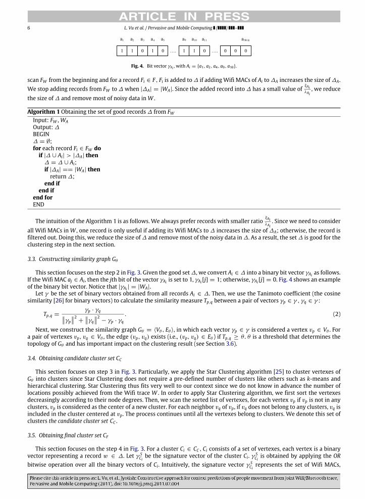
Fig. 4. Bit vector γAi , with Ai = a1, a2, a4, a9, a10.

scan FW from the beginning and for a record Fi ∈ F , Fi is added to ∆ if addingWifi MACs of Ai to ∆A increases the size of ∆A.We stop adding records from FW to ∆ when |∆A| = |WA|. Since the added record into ∆ has a small value of

ξAiλAi

, we reducethe size of ∆ and remove most of noisy data inW .

Algorithm 1 Obtaining the set of good records ∆ from FWInput: FW , WAOutput: ∆

BEGIN∆ = ∅;for each record Fi ∈ FW do

if |∆ ∪ Ai| > |∆A| then∆ = ∆ ∪ Ai;if |∆A| == |WA| then

return ∆;end if

end ifend forEND

The intuition of the Algorithm 1 is as follows. We always prefer records with smaller ratioξAiλAi

. Since we need to considerall Wifi MACs in W , one record is only useful if adding its Wifi MACs to ∆ increases the size of ∆A; otherwise, the record isfiltered out. Doing this, we reduce the size of ∆ and remove most of the noisy data in ∆. As a result, the set ∆ is good for theclustering step in the next section.

3.3. Constructing similarity graph Gθ

This section focuses on the step 2 in Fig. 3. Given the good set ∆, we convert Ai ∈ ∆ into a binary bit vector γAi as follows.If theWifi MAC aj ∈ Ai, then the jth bit of the vector γAi is set to 1, γAi [j] = 1; otherwise, γAi [j] = 0. Fig. 4 shows an exampleof the binary bit vector. Notice that |γAi | = |WA|.

Let γ be the set of binary vectors obtained from all records Ai ∈ ∆. Then, we use the Tanimoto coefficient (the cosinesimilarity [26] for binary vectors) to calculate the similarity measure Tp,q between a pair of vectors γp ∈ γ , γq ∈ γ :

Tp,q =γp · γqγp

2+

γq2

− γp · γq

. (2)

Next, we construct the similarity graph Gθ = ⟨Vθ , Eθ ⟩, in which each vector γp ∈ γ is considered a vertex vp ∈ Vθ . Fora pair of vertexes vp, vq ∈ Vθ , the edge (vp, vq) exists (i.e., (vp, vq) ∈ Eθ ) if Tp,q ≥ θ . θ is a threshold that determines thetopology of Gθ and has important impact on the clustering result (see Section 3.6).

3.4. Obtaining candidate cluster set CC

This section focuses on step 3 in Fig. 3. Particularly, we apply the Star Clustering algorithm [25] to cluster vertexes ofGθ into clusters since Star Clustering does not require a pre-defined number of clusters like others such as k-means andhierarchical clustering. Star Clustering thus fits very well to our context since we do not know in advance the number oflocations possibly achieved from the Wifi trace W . In order to apply Star Clustering algorithm, we first sort the vertexesdecreasingly according to their node degrees. Then, we scan the sorted list of vertexes, for each vertex vp if vp is not in anyclusters, vp is considered as the center of a new cluster. For each neighbor vq of vp, if vq does not belong to any clusters, vq isincluded in the cluster centered at vp. The process continues until all the vertexes belong to clusters. We denote this set ofclusters the candidate cluster set CC .

3.5. Obtaining final cluster set CF

This section focuses on the step 4 in Fig. 3. For a cluster Ci ∈ CC , Ci consists of a set of vertexes, each vertex is a binaryvector representing a record w ∈ ∆. Let γ S

Cibe the signature vector of the cluster Ci. γ S

Ciis obtained by applying the OR

bitwise operation over all the binary vectors of Ci. Intuitively, the signature vector γ SCi

represents the set of Wifi MACs,


Table 5Example of table F .

Scan time Wifi MACs Loc

03/08/10 09:20 a1, a3 L103/08/10 09:50 a1, a5 L103/08/10 10:20 a6 L503/08/10 13:50 a4, a7, a9 L803/14/10 08:20 a1, a3 L1

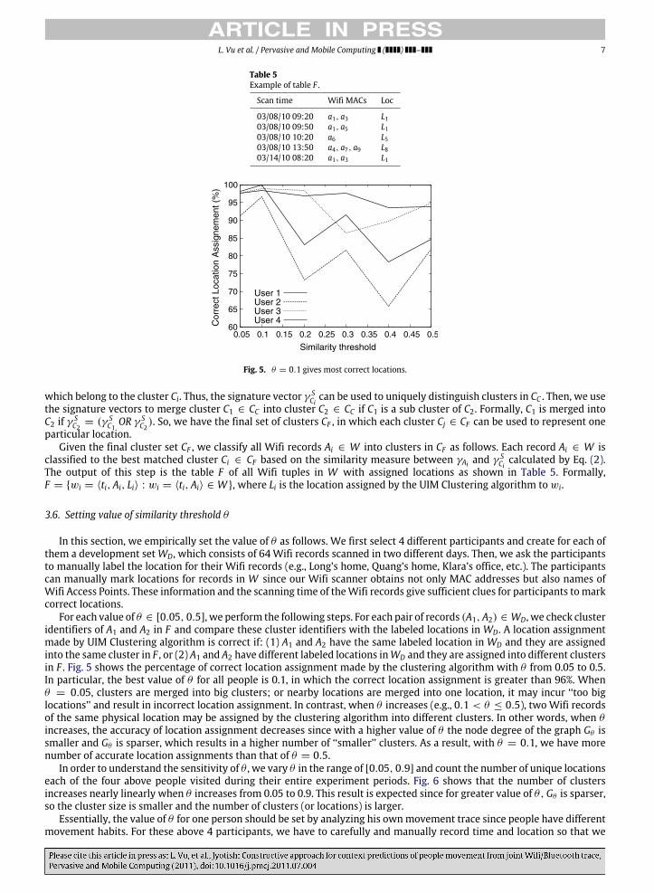
Fig. 5. θ = 0.1 gives most correct locations.

which belong to the cluster Ci. Thus, the signature vector γ SCican be used to uniquely distinguish clusters in CC . Then, we use

the signature vectors to merge cluster C1 ∈ CC into cluster C2 ∈ CC if C1 is a sub cluster of C2. Formally, C1 is merged intoC2 if γ S

C2= (γ S

C1OR γ S

C2). So, we have the final set of clusters CF , in which each cluster Cj ∈ CF can be used to represent one

particular location.Given the final cluster set CF , we classify all Wifi records Ai ∈ W into clusters in CF as follows. Each record Ai ∈ W is

classified to the best matched cluster Ci ∈ CF based on the similarity measure between γAi and γ SCi

calculated by Eq. (2).The output of this step is the table F of all Wifi tuples in W with assigned locations as shown in Table 5. Formally,F = wi = ⟨ti, Ai, Li⟩ : wi = ⟨ti, Ai⟩ ∈ W , where Li is the location assigned by the UIM Clustering algorithm to wi.

3.6. Setting value of similarity threshold θ

In this section, we empirically set the value of θ as follows. We first select 4 different participants and create for each ofthem a development setWD, which consists of 64 Wifi records scanned in two different days. Then, we ask the participantsto manually label the location for their Wifi records (e.g., Long’s home, Quang’s home, Klara’s office, etc.). The participantscan manually mark locations for records in W since our Wifi scanner obtains not only MAC addresses but also names ofWifi Access Points. These information and the scanning time of theWifi records give sufficient clues for participants tomarkcorrect locations.

For each value of θ ∈ [0.05, 0.5], we perform the following steps. For each pair of records (A1, A2) ∈ WD, we check clusteridentifiers of A1 and A2 in F and compare these cluster identifiers with the labeled locations in WD. A location assignmentmade by UIM Clustering algorithm is correct if: (1) A1 and A2 have the same labeled location in WD and they are assignedinto the same cluster in F , or (2) A1 and A2 have different labeled locations inWD and they are assigned into different clustersin F . Fig. 5 shows the percentage of correct location assignment made by the clustering algorithm with θ from 0.05 to 0.5.In particular, the best value of θ for all people is 0.1, in which the correct location assignment is greater than 96%. Whenθ = 0.05, clusters are merged into big clusters; or nearby locations are merged into one location, it may incur ‘‘too biglocations’’ and result in incorrect location assignment. In contrast, when θ increases (e.g., 0.1 < θ ≤ 0.5), two Wifi recordsof the same physical location may be assigned by the clustering algorithm into different clusters. In other words, when θincreases, the accuracy of location assignment decreases since with a higher value of θ the node degree of the graph Gθ issmaller and Gθ is sparser, which results in a higher number of ‘‘smaller’’ clusters. As a result, with θ = 0.1, we have morenumber of accurate location assignments than that of θ = 0.5.

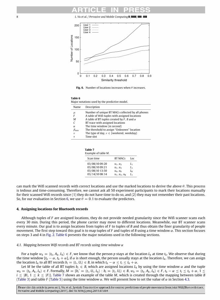
In order to understand the sensitivity of θ , we vary θ in the range of [0.05, 0.9] and count the number of unique locationseach of the four above people visited during their entire experiment periods. Fig. 6 shows that the number of clustersincreases nearly linearly when θ increases from 0.05 to 0.9. This result is expected since for greater value of θ,Gθ is sparser,so the cluster size is smaller and the number of clusters (or locations) is larger.

Essentially, the value of θ for one person should be set by analyzing his ownmovement trace since people have differentmovement habits. For these above 4 participants, we have to carefully and manually record time and location so that we


Fig. 6. Number of locations increases when θ increases.

Table 6Major notations used by the predictive model.

Name Description

µ Number of unique BT MACs collected by all phonesF A table of Wifi tuples with assigned locationsM A table of BT tuples created by F , B and α

C BT trace with assigned locationsα The time window (in second)βmin The threshold to assign ‘‘Unknown’’ locationν The type of day, ν ∈ weekend,weekdayτ Time slot

Table 7Example of table M .

Scan time BT MACs Loc

03/08/10 09:20 u1, u3 L103/08/10 09:21 u1, u3 L103/08/10 13:50 u4, u9 L803/14/10 08:14 u1, u3, u8 L1

can mark the Wifi scanned records with correct locations and use the marked locations to derive the above θ . This processis tedious and time-consuming. Therefore, we cannot ask all 50 experiment participants to mark their locations manuallyfor their scannedWifi records since (1) they do not have time to do so, and (2) they may not remember their past locations.So, for our evaluation in Section 6, we use θ = 0.1 to evaluate the predictors.

4. Assigning locations for Bluetooth records

Although tuples of F are assigned locations, they do not provide needed granularity since the Wifi scanner scans eachevery 30 min. During this period, the phone carrier may move to different locations. Meanwhile, our BT scanner scansevery minute. Our goal is to assign locations from tuples of F to tuples of B and thus obtain the finer granularity of peoplemovement. The first step toward this goal is to map tuples of F and tuples of B using a time window α. This section focuseson steps 3 and 4 in Fig. 2. Table 6 presents the major notations used in the following sections.

4.1. Mapping between Wifi records and BT records using time window α

For a tuple wk = ⟨tk, Ak, Lk⟩ ∈ F , we know that the person p stays at the location Lk at time tk. We observe that duringthe time window [tk − α, tk + α], if α is short enough, the person usually stays at the location Lk. Therefore, we can assignthe location Lk to all BT records bi = ⟨ti,Ui⟩ ∈ B, in which tk − α ≤ ti ≤ tk + α.

Let M be the table of all BT tuples bi ∈ B, which are assigned locations Lk by using the time window α and the tuplewk = ⟨tk, Ak, Lk⟩ ∈ F . Formally, M = bi′ = ⟨ti,Ui, Lk⟩ : bi = ⟨ti,Ui⟩ ∈ B, wk = ⟨tk, Ak, Lk⟩ ∈ F , tk − α ≤ ti ≤ tk + α, 1 ≤

i ≤ |B|, 1 ≤ k ≤ |F |. Table 7 shows an example of the table M , which is created through the mapping between table B(Table 3) and table F (Table 5) using the time window α. We will present how to set the value of α in Section 4.3.


4.2. Assigning locations for Bluetooth records

We construct a Naive Bayesian classifier NB to predict the locations of all BT records in B. Basically, we use the tableM totrain the Naive Bayesian classifier NB and then use NB to assign locations to all records bi ∈ B.

4.2.1. Training Naive Bayesian classifier NB

For a BT record bi ∈ B, the probability that bi belongs to a location Lk is calculated by using the Bayesian Theorem asfollows:

P(Lk|bi) =P(bi|Lk)P(Lk)

P(bi). (3)

Then, bi belongs to the location Lbi calculated as follows:

Lbi = arg maxk

P(bi|Lk)P(Lk)P(bi)

. (4)

Since P(bi) is the same for all locations Lk, we calculate f (Lk) = P(bi|Lk)P(Lk). To calculate P(bi|Lk), we assume that foru1 ∈

bi3 and u2 ∈ bi, u1 and u2 are conditionally independent, or u1 and u2 appear conditionally independent in the proximity ofthe experiment phone when they are scanned (and bi is created) by the BT scanner. This assumption usually holds in realitysince people (with their Bluetooth-enable devices) appear at locations independently.4 Let f (Lk) = Πuj∈biP(uj|Lk)P(Lk), wehave:

Lbi = arg maxk

f (Lk). (5)

The tableM is used to calculate f (Lk) in Eq. (5) as follows. P(Lk) =c(Lk)|M|

, where |M| is the size ofM and c(Lk) is the numberof tuples bi′ = ⟨ti,Ui, Li⟩ ∈ M , in which Li = Lk. For P(uj|Lk), we have:

P(uj|Lk) =c(uj)

c(Lk). (6)

In Eq. (6), c(uj) is the number of records bi′ = ⟨ti,Ui, Li⟩ ∈ M , in which Li = Lk and uj ∈ Ui. Applying Eqs. (5) and (6) forall records ofM , we have the trained classifier NB.

4.2.2. Applying additive smoothing techniqueIn Section 4.1, since we only use a small time window α to create M,M does not cover all BT MACs in B. Thus, applying

the trained classifier NB for a record bi ∈ B, the value c(uj) in Eq. (6) might be 0 if uj does not belong to any tuples of M .Thus, c(uj) cancels out the value of P(ul|Lk) of BT MACs ul ∈ bi (i.e., j = l) in Eq. (5). To avoid this, we apply the AdditiveSmoothing technique [27] for Eq. (6) as follows:

P(uj|Lk) =c(uj) + 1c(Lk) + µ

. (7)

In Eq. (7), µ is the number of unique BT MACs collected by all participants for the entire experiment period from Marchto August 2010. Adding µ to the denominator of Eq. (7) means we take into account all possible BT MACs in calculating theprobability of the BT MAC uj. With Eq. (7), P(uj|Lk) = 0 for all uj and we have:

f (Lk) = Πuj∈bic(uj) + 1c(Lk) + µ

P(Lk). (8)

So, we have a new trained classifier N ′

B by applying Eqs. (5) and (8) for all tuples ofM .

4.2.3. The ‘‘Unknown’’ locationApplying N ′

B to assign locations to BT records bi ∈ B, we encounter records bi whose value of f (Lbi) calculated by Eqs. (4)and (7) is extremely small. These records bi are scanned in the middle of two consecutive Wifi scans (the period betweentwo Wifi scans is 30 min) when the phone carrier moves to another location, which is not captured by the Wifi scanner.Therefore, assigning any known location from the Wifi trace to bi results in a wrong assignment. To avoid this, we define anew location named ‘‘Unknown’’ location and assign the ‘‘Unknown’’ location to bi.

3 The correct notation should be u1 ∈ Ui and bi = ⟨ti,Ui⟩. However, to shorten the notation, we use u1 ∈ bi in this section.4 We are aware that this assumption will not hold if a group of people move together. However, we believe that themovement of group is not as popular

as the movement of individual in working environment.


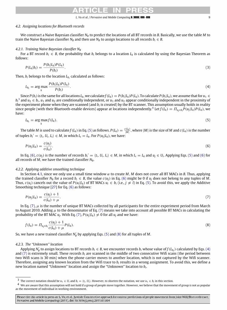
Fig. 7. Time window α = 60(s) gives most correct locations.

The next question is ‘‘How small the value of f (Lbi) is’’ so that the record bi is assigned to ‘‘Unknown’’ location. To answerthis question, we use Eq. (8) to calculate f (Lbi ′) for all records bi

′∈ M . Let βmin = minbi ′∈M f (Lbi). We then use βmin as the

threshold value to assign ‘‘Unknown’’ location to a BT record bi ∈ B. The intuition is as follows. We assume that records inM are ‘‘good records’’ whose locations are assigned correctly by the time window α. So, the minimum value of f (Lbi ′) of allrecords bi′ ∈ M represents the cutoff value for all records whose locations are assigned correctly. For a record bi ∈ B, wehave:

Lbi =

arg max

if (Lk) if f (Lbi) ≥ βmin

‘‘Unknown’’ otherwise.(9)

Eq. (9) means bi will be assigned Lbi location only if f (Lbi) ≥ βmin. Otherwise, bi will be assigned the ‘‘Unknown’’ location.Although this approach seems to be conservative in assigning correct locations to BT records, it does provide good resultin our evaluation of the predictive model in Section 6. Let C be the table consisting of all records in B, which are assignedlocations. Then, we sort C increasingly according to the scan times of its tuples and use C as the input to construct ourpredictors in Section 5.

4.3. Setting value of time window α

As we presented in Section 4.1, the value of α decides the mapping between Wifi records and BT records and the size oftable M , which is used to train the Naive Bayesian classifier NB. In this section, we use the same technique in Section 3.6 toempirically set value for α.

Particularly, we select 4 participants and for each of them, we create a set BD of BT records of two days and ask theparticipants to manually label locations for records in his BD. For two days, each BD has 960 records. The participants canmanually mark locations for records in B since our BT scanner obtains not only MAC addresses but also names of Bluetooth-enabled devices. These information and the scanning time of the BT records give sufficient clues for participants to markcorrect locations.

For each pair of records (b1, b2) ∈ BD, we check locations of b1 and b2 in C assigned by our Naive Bayesian classifier andcompare these locations with the labeled locations in BD. Fig. 7 shows that when α = 60(s), the table C outputted by theNaive Bayesian classifier obtains the best location assignment, in which the correct prediction for all 4 people is greater than95%.With α = 30(s), the tableM consists of too few records to train a good Naive Bayesian classifier. Meanwhile, α > 60(s)is too large a time window, which incurs noisy data in the table M since BT records may be assigned wrong locations ifthey fall into this big time window. The trained classifier NB then performs worse with α = 60(s). So, we use α = 60(s) toevaluate the performance of our predictive model in Section 6.

5. Constructing location predictor, duration predictor, and contact predictor

Given the table C , we construct the location predictor, duration predictor, and contact predictor. This section focuseson step 5 and step 6 in Fig. 2. To construct our predictors, we use two parameters: type of day and time slot. Let νbe the ‘‘type of day’’ and τ be the ‘‘time slot’’. Particularly, we classify days into two types: weekend and weekday, soν ∈ weekday,weekend, and divide time of a day into time slot of size 1, 2, 4, etc. hours. The motivation for the use ofthese two parameters is that people may visit different places and contact different people for the weekday and weekend.For each record r ∈ C , we map r ’s scan time into type of day ν and time slot τ . Table 8 shows an example of the table C inwhich its tuples are mapped into type of day and time slot of size 2 hours. The table C in this new format is used to constructour predictors.


Table 8Example of BT trace with assigned location C .

ν τ Scan time Loc BT MACs

Weekday 08–10 03/08/10 09:20 L1 u1, u3Weekday 08–10 03/08/10 09:21 L1 u1, u3Weekday 08–10 03/08/10 09:22 L1 u1, u8Weekday 12–14 03/08/10 13:50 L8 u4, u9Weekend 08–10 03/14/10 08:12 L8 u4, u12Weekday 08–10 03/15/10 09:47 L1 u1Weekend 14–16 03/20/10 15:23 L3 u15

For a person p, the input query for p’s movement prediction is a record X in the format of X = ν1, τX , in which νXrepresents the type of day and τX represents the time slot. The output will be location p stays at, the duration p stays at thelocation, and contacts p has for the type of day νX and during time slot τX .

5.1. Location predictor

We use the Bayesian classifier to predict the location of the person as follows.

LX = arg maxi

P(ν = νX , τ = τX |Li)P(Li). (10)

Eq. (10) outputs the most likely location LX for the input query X . Moreover, Eq. (10) can be easily customized to returnthe top-k of the most likely locations for the input query X . In this case, LX is the set of top-k most likely locations and wehave a top-k location predictor.

In Eq. (10), we do not assume the conditional independence between ν = νX and τ = τX as presented in [21], since inreality a person may visit different locations in the weekdays and weekend for the same time slot. For example, in the timeslot from 9 AM to 11 AM, the person may stay in the office in her workplace for the weekdays but she may be at home atthe weekend.

5.2. Duration predictor

The duration predictor is constructed based on the location predictor. If the location predictor returns the top-k locations,the duration predictor will return the predicted stay duration for each of k locations.

We first define the ‘‘stay session at the location Lk’’ is the continuous time period that the person stays at Lk. In our context,since the BT scanner obtains BT records every minute, the ‘‘stay session at the location Lk in minute’’ is the size of the table Φ

of consecutive tuples in table C such that for two consecutive tuples r1, r2 ∈ Φ , the difference of scan times between r1 and r2 isexactly 1 min. Let |Φ| denote the session length of one stay session of Lk.

We first use location predictor to obtain the location Lk for the input query X = (νX , τX ). Then, we create a sub tableC ′ by selecting all records of C , which has ν = νX , τ = τX , and Loc = Lk. Then, we calculate the session lengths for Lkfrom the table C ′ using the above session definition. Let Γk be the set of all stay session lengths for the location Lk obtainedfrom table C ′, Γk = Φ1, Φ2, Φ3, . . . , Φ|Γk|, Γk forms a distribution of session lengths. Let λk and ξk denote the mean andstandard deviation of this distribution. For example, the location L1 in Table 8 has Γ1 = 3, 1, here |Φ1| = 3 and |Φ2| = 1(Φ1 consists of the first three records). The output of the duration predictor includes λk, and ξk for each location Lk.

On the one hand, the duration predictor can predict how long the person stays at one location. On the other hand, sinceour location is inferred from the collected Wifi access point trace, the duration predictor essentially predicts the potentialwireless connection opportunity. Thus, the duration predictor can be used as the fundamental building block for the designof network protocols in mobile wireless networks.

5.3. Contact predictor

In order to construct the contact predictor, we assume that each BT MAC scanned by the BT scanner is associated witha distinct person. As a result, each scanned BT MAC in a record of the BT trace represents a contact. We apply the Bayesianclassifier to find the most likely contact the person p will have for the input X = νX , τX as follows:

UX = arg maxj

P(ν = νX , τ = τX |uj)P(uj). (11)

Eq. (11) outputs the most likely contact UX for the input query X . Eq. (11) can be easily customized to return the top-kof the most likely contacts for the input query X . In this case, UX is the set of top-kmost likely contacts and we have a top-kcontact predictor. The contact predictor predicts the future contacts, which is crucial for the design of routing protocols andcontent distribution protocols in MANET and DTN [28].

Note that in Eq. (11), we do not assume the conditional independence between ν = νX and τ = τX as presented in [21],since in reality a personmaymeet different sets of people in theweekdays andweekend for the same time slot. For example,


Fig. 8. Location predictor.

in the time slot from 2 PM to 4 PM, the person may meet friends in class for the weekdays but she may meet his familymembers at the weekend.

6. Evaluation of the predictive model

6.1. Evaluation settings

We take 50 joint Wifi/Bluetooth traces from the entire set of traces as shown in Table 1. Each selected trace is from 20to 50 days. Let Di be the Wifi/Bluetooth trace of the ith participant in 50 participants: Di = Wi ∪ Bi, where Wi is the Wifitrace and Bi is the BT trace. For ith participant, we first apply the UIM Clustering Algorithm overWi to obtain locations. Then,we apply steps in Section 4 to assign locations to records in Bi. For the ith user, let Ci be the Bluetooth trace with assignedlocation. We divide the table Ci into two distinct sub sets called training set Ψi and testing set Ωi, in which Ψi ∩ Ωi = ∅.The training set Ψi has 80% of records in Ci and Ωi has 200 records randomly picked from the set Ci \ Ψi. We use Ψi to trainthree predictors (i.e., location, stay duration, and contact) and use Ωi to evaluate these predictors. Each record r ∈ Ωi isconverted into the format of X = νX , τX and used as the input for our predictors. We set θ = 0.1, α = 60(s), and time slotto 2 h in the following plots. We run the experiment 20 times (i.e., each time a new set Ωi is created at random) and plotthe average with the 95% confident interval. Notice that results in this section are new in comparison with results presentedin [21] since we take into account of non-independent assumptions in Eqs. (10) and (11).

6.2. Correctness of predictors

6.2.1. Location predictorLet Lip be the location predictor of the ith experiment participant. For each record r ∈ Ωi, we use Lip to predict the location

of r using technique in Section 5.1. Let Lr be the location of r ∈ Ωi. Notice that we only evaluate the correctness of Lip forrecord r whose Lr is not ‘‘Unknown’’. Since the predictor Lip can output the top-kmost likely locations, let Lpred be the set ofpredicted locations outputted by Lip so |Lpred| = k. Lip makes a correct prediction if Lr ⊆ Lpred.

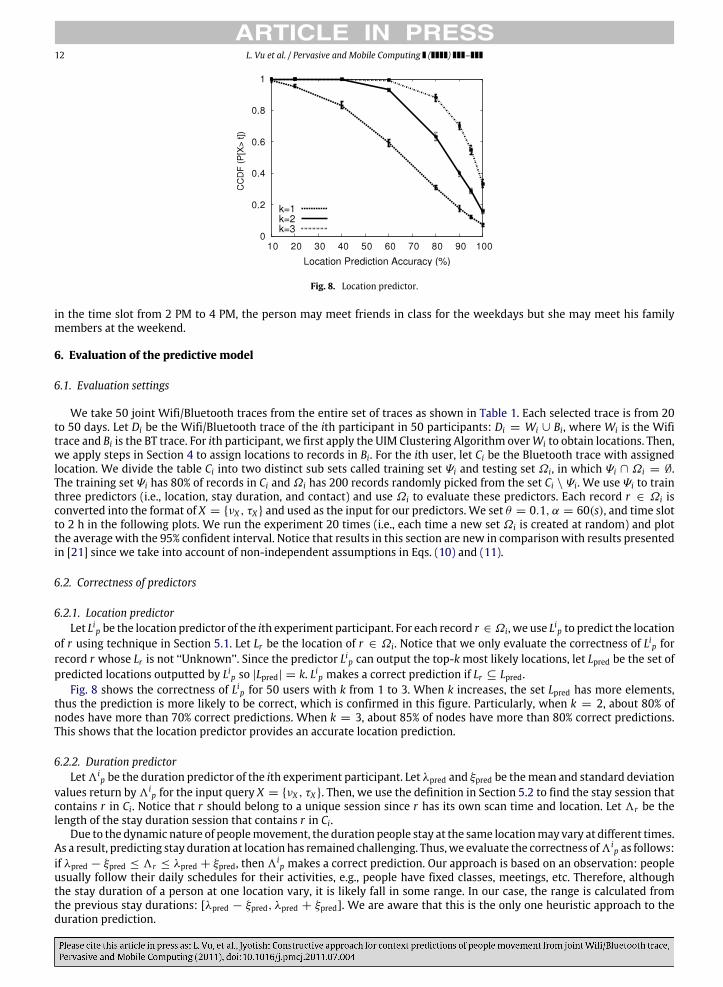
Fig. 8 shows the correctness of Lip for 50 users with k from 1 to 3. When k increases, the set Lpred has more elements,thus the prediction is more likely to be correct, which is confirmed in this figure. Particularly, when k = 2, about 80% ofnodes have more than 70% correct predictions. When k = 3, about 85% of nodes have more than 80% correct predictions.This shows that the location predictor provides an accurate location prediction.

6.2.2. Duration predictorLet3i

p be the duration predictor of the ith experiment participant. Let λpred and ξpred be themean and standard deviationvalues return by 3i

p for the input query X = νX , τX . Then, we use the definition in Section 5.2 to find the stay session thatcontains r in Ci. Notice that r should belong to a unique session since r has its own scan time and location. Let 3r be thelength of the stay duration session that contains r in Ci.

Due to the dynamic nature of peoplemovement, the duration people stay at the same locationmay vary at different times.As a result, predicting stay duration at location has remained challenging. Thus,we evaluate the correctness of3i

p as follows:if λpred − ξpred ≤ 3r ≤ λpred + ξpred, then 3i

p makes a correct prediction. Our approach is based on an observation: peopleusually follow their daily schedules for their activities, e.g., people have fixed classes, meetings, etc. Therefore, althoughthe stay duration of a person at one location vary, it is likely fall in some range. In our case, the range is calculated fromthe previous stay durations: [λpred − ξpred, λpred + ξpred]. We are aware that this is the only one heuristic approach to theduration prediction.


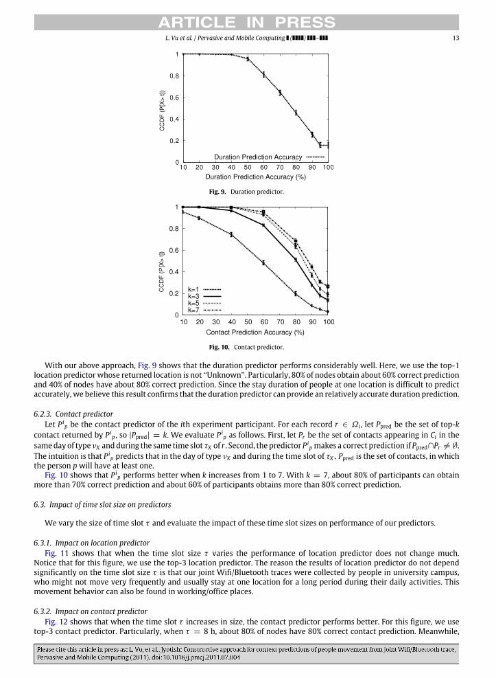
Fig. 9. Duration predictor.

Fig. 10. Contact predictor.

With our above approach, Fig. 9 shows that the duration predictor performs considerably well. Here, we use the top-1location predictor whose returned location is not ‘‘Unknown’’. Particularly, 80% of nodes obtain about 60% correct predictionand 40% of nodes have about 80% correct prediction. Since the stay duration of people at one location is difficult to predictaccurately, we believe this result confirms that the duration predictor can provide an relatively accurate duration prediction.

6.2.3. Contact predictorLet P i

p be the contact predictor of the ith experiment participant. For each record r ∈ Ωi, let Ppred be the set of top-kcontact returned by P i

p, so |Ppred| = k. We evaluate P ip as follows. First, let Pr be the set of contacts appearing in Ci in the

sameday of type νX andduring the same time slot τX of r . Second, the predictor P ip makes a correct prediction if Ppred∩Pr = ∅.

The intuition is that P ip predicts that in the day of type νX and during the time slot of τX , Ppred is the set of contacts, in which

the person p will have at least one.Fig. 10 shows that P i

p performs better when k increases from 1 to 7. With k = 7, about 80% of participants can obtainmore than 70% correct prediction and about 60% of participants obtains more than 80% correct prediction.

6.3. Impact of time slot size on predictors

We vary the size of time slot τ and evaluate the impact of these time slot sizes on performance of our predictors.

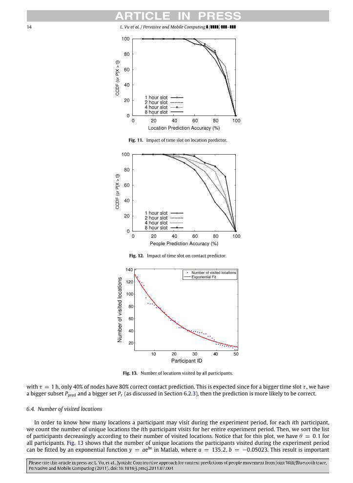
6.3.1. Impact on location predictorFig. 11 shows that when the time slot size τ varies the performance of location predictor does not change much.

Notice that for this figure, we use the top-3 location predictor. The reason the results of location predictor do not dependsignificantly on the time slot size τ is that our joint Wifi/Bluetooth traces were collected by people in university campus,who might not move very frequently and usually stay at one location for a long period during their daily activities. Thismovement behavior can also be found in working/office places.

6.3.2. Impact on contact predictorFig. 12 shows that when the time slot τ increases in size, the contact predictor performs better. For this figure, we use

top-3 contact predictor. Particularly, when τ = 8 h, about 80% of nodes have 80% correct contact prediction. Meanwhile,


Fig. 11. Impact of time slot on location predictor.

Fig. 12. Impact of time slot on contact predictor.

Fig. 13. Number of locations visited by all participants.

with τ = 1 h, only 40% of nodes have 80% correct contact prediction. This is expected since for a bigger time slot τ , we havea bigger subset Ppred and a bigger set Pr (as discussed in Section 6.2.3), then the prediction is more likely to be correct.

6.4. Number of visited locations

In order to know how many locations a participant may visit during the experiment period, for each ith participant,we count the number of unique locations the ith participant visits for her entire experiment period. Then, we sort the listof participants decreasingly according to their number of visited locations. Notice that for this plot, we have θ = 0.1 forall participants. Fig. 13 shows that the number of unique locations the participants visited during the experiment periodcan be fitted by an exponential function y = aebx in Matlab, where a = 135.2, b = −0.05023. This result is important


since it gives a concrete model for the number of locations for mobile nodes, which can be used for simulation purpose inmobile networking research. Particularly, instead of taking a random number as the number of locations for a mobile nodein simulations, researchers might take a number following an exponential function as shown in Fig. 13.

7. Conclusion

Jyotish framework provides an efficient solution to construct a predictive model of people movement from jointWifi/Bluetooth trace. Evaluation over the Wifi/Bluetooth trace collected by 50 participants shows that the constructedpredictive model predicts location, stay duration, and contact with a considerably high accuracy.

To the best of our knowledge, Jyotish framework is the first to derive a predictive model from a real joint Wifi/Bluetoothtrace. The constructed model is also the first to provide prediction of location, stay duration, and contact altogether. Sincefuture knowledge of people movement is fundamental for numerous domains such as mobile wireless networks, HCI,social science, environmental science, etc., we thus believe Jyotish framework and its derived predictive model are widelyapplicable.

References

[1] M.C. Gonzalez, C.A. Hidalgo, A.-L. Barabasi, Understanding individual human mobility pattern, Nature 453 (2008) 779–782.[2] G. Liu, G. Maguire, A class of mobile motion prediction algorithms for wireless mobile computing and communications, Mobile Networks and

Applications 1 (1996) 113–121.[3] W. Gao, G. Gao, Fine-grained mobility characterization: steady and transient state behaviors, in: Proceedings of Mobihoc, 2010.[4] L. Song, D. Kotz, R. Jain, X. He, Evaluating location predictors with extensive Wi-Fi mobility data,

in: Proceedings of Infocom, 2004.[5] M. Sun, D. Blough, Mobility prediction using future knowledge, in: Proceedings of MSWiM, 2007.[6] W. Hsu, T. Spyropoulos, K. Psounis, A. Helmy, Modeling time-variant user mobility in wireless mobile networks, in: Proceedings of Infocom, 2007.[7] R. Jain, A. Shivaprasad, D. Lelescu, X. He, Towards a model of user mobility and registration patterns, ACM SIGMOBILE Mobile Computing and

Communications Review 8 (2004) 59–62.[8] J.-K. Lee, J.C. Hou, Modeling steady-state and transient behaviors of user mobility: formulation, analysis, and application, in: Proceedings of Mobihoc,

2006.[9] M. Balazinska, P. Castro, Characterizing mobility and network usage in a corporate wireless local-area network, in: Proceedings of Mobisys, 2003.

[10] T. Henderson, D. Kotz, I. Abyzov, The changing usage of a mature campus-wide wireless network, in: Proceedings of Mobicom, 2004.[11] P.N. Pathirana, A.V. Savkin, S. Jha, Mobility modelling and trajectory prediction for cellular networks with mobile base stations, in: Proceedings of

MobiHoc, 2003.[12] M.A. Bayira, M. Demirbasa, Mobility profiler: a framework for discovering mobility profiles of cell phone users, Pervasive and Mobile Computing

(2010).[13] L. McNamara, C. Mascolo, L. Capra, Media sharing based on colocation prediction in urban transport, in: Proceedings of Mobicom, 2008.[14] S. Scellato, M. Musolesi, C. Mascolo, V. Latora, A. Campbell, Nextplace: a spatio-temporal prediction framework for pervasive systems, in: Proceedings

of Ninth International Conference on Pervasive Computing, 2011.[15] A. Chaintreau, P. Hui, J. Crowcroft, C. Diot, R. Gass, J. Scott, Impact of human mobility on the design of opportunistic forwarding algorithms, in:

Proceedings of Infocom, 2006.[16] P. Hui, A. Chaintreau, J. Scott, R. Gass, J. Crowcroft, C. Diot, Pocket switched networks and humanmobility in conference environments, in: Proceedings

of the ACM SIGCOMMWorkshop on Delay-Tolerant Networking, 2005.[17] J. Leguay, A. Lindgren, J. Scott, T. Friedman, J. Crowcroft, Opportunistic content distribution in an urban setting, in: Proceedings of CHANTS, 2006.[18] E.P.S. Gaito, G.P. Rossi, Opportunistic forwarding in workplaces, in: Proceedings of ACMWOSN, 2009.[19] P.-U. Tournoux, J. Leguay, F. Benbadis, V. Conan, M.D. de Amorim, J. Whitbeck, The accordion phenomenon: analysis, characterization, and impact on

DTN routing, in: Proceedings of IEEE Infocom, 2010.[20] L. Vu, K. Nahrstedt, S. Retika, I. Gupta, Joint Bluetooth/Wifi scanning framework for characterizing and leveraging people movement in university

campus, in: Proceedings of MSWiM, 2010.[21] L. Vu, Q. Do, K. Nahrstedt, Jyotish: a novel framework for constructing prediction model of people movement from joint Wifi/Bluetooth trace, in:

Proceedings of Percom, 2011.[22] Skyhook. http://www.skyhookwireless.com.[23] J. Krumm, K. Hinckley, The nearme wireless proximity server, in: Proceedings of Ubicomp, 2004.[24] A. LaMarca, J. Hightower, I. Smith, S. Consolvo, Self-mapping in 802.11 location systems, in: Proceedings of Ubicomp, 2005.[25] J. Aslam, K. Pelekhov, D. Rus, Static and dynamic information organization with star clusters, in: Proceedings of the Conference on Information

Knowledge Management, 1998, pp. 208–217.[26] J. Han, M. Kamber, Data Mining: Concepts and Techniques, 2nd ed., Morgan Kaufmann Publishers, 2001, pp. 225–276.[27] C.D. Manning, H. Schütze, Foundations of Statistical Natural Language Processing, MIT Press, Cambridge, MA, USA, 1999.[28] L. Vu, Q. Do, K. Nahrstedt, 3R: fine-grained encounter-based routing in delay tolerant networks, in: Proceedings of 12th IEEE International Symposium

on a World of Wireless, Mobile and Multimedia Networks, WoWMoM, 2011.

http://www.skyhookwireless.com

Jyotish: Constructive approach for context predictions of ...

Documents

Transcript of Jyotish: Constructive approach for context predictions of ...