A Constructive Approach to Hardware/Software Partitioning

Formal Methods in System Design, 24, 45–90, 2004c© 2004 Kluwer Academic Publishers. Manufactured in The Netherlands.

A Constructive Approachto Hardware/Software Partitioning

LEILA SILVA [email protected] de Ciencia da Computacao e Estatıstica, Universidade Federal de Sergipe, Campus Universitario“Prof. Jose Aloısio Campos”, CEP 49100-000, Sao Cristovao, SE, Brazil

AUGUSTO SAMPAIO [email protected] BARROS [email protected] de Informatica, Universidade Federal de Pernambuco, Caixa Postal 7851, Cidade Universitaria,CEP 50732-970 Recife, PE, Brazil

Received November 14, 2001; Revised April 1, 2003; Accepted June 20, 2003

Abstract. A crucial point in hardware/software co-design is how to perform the partitioning of a system intohardware and software components. Although several algorithms to partitioning have been recently proposed,the formal verification of the partitioning procedure is an emergent research topic. In this paper we present aninnovative and automatic approach to partitioning with emphasis on correctness. The formalism used is occam andthe algebraic laws that define its semantics. In the proposed approach, the partitioning procedure is characterisedas a program transformation task and the partitioned system is derived from the original description of the systemby applying transformation rules, all of them proved from the basic laws of occam. A tool has been developed toallow the partitioning to be carried out automatically. The entire approach is illustrated here through a small casestudy.

Keywords: co-design, hardware/software partitioning, formal verification, algebraic laws, occam

1. Introduction

Embedded systems are dedicated to a specific target application and the majority of themare implemented using general programmable (software) components and specific appli-cation (hardware) components. They can be found in a large variety of applications suchas telecommunication systems, intelligent home devices, and in systems for the defence ofterritory and the environment.

Hardware/Software co-design or simply co-design is a new design paradigm for the jointspecification, design and synthesis of mixed hardware/software systems. The interest inautomatic co-design techniques is driven by the increasing diversity and complexity ofapplications employing embedded systems and the need for a decreasing cost in the designand test of hardware/software systems, with the aim of reducing the time-to-market.

In the last years several methodologies and tools supporting hardware/software co-designfor embedded systems have been published (among them, we single out the approachespresented in [9, 11, 15, 23]). The typical flow of co-design, which is common to most ofthe approaches published in the literature, is given in figure 1.

46 SILVA, SAMPAIO AND BARROS

Figure 1. Typical co-design methodology.

Basically, the application is specified in a high-level language (such as C or VHDL [17])and after that it is translated into an internal model of representation (for example, graphs[9] or finite state machines [15]). Next, in the partitioning phase, a systematic procedureis applied to decide which parts of the system will be implemented in a software or ina hardware component, as well as the way the processes into each component should becombined (in sequence or in parallel). Then, the software description is compiled andthe hardware is synthesised. The interface among hardware and software components isalso synthesised. The results of the compilation and the synthesis phases are integratedinto a prototyping platform. The hardware and interface components are coupled with aprocessor that executes the software partition. Finally, the application is co-simulated andif the tests are successful, the chip is designed, giving rise to a physical implementation. Allphases of the co-design flow involve system transformations; thus, system verification isfundamental to ensure that the original behaviour of the specification is preserved in thesephases. Validation is also crucial to ensure that the initial specification does embody somedesired properties, such as deadlock freedom.

This work focuses on the formal verification of the partitioning procedure. Partitioningis a well-known NP-complete problem and recently many heuristics have been proposedto guide the partitioning of a system into hardware and software components (see, forexample, [2, 21, 24, 26]). These approaches validate the partitioned system by simulation(for instance, [9, 11, 23]) or by using formal methods to prove that some desired propertiesof the original system are preserved after partitioning [15, 16]. In particular, the validationapproach of POLIS [15] separates the concerns of functional correctness and timing, anidea also explored in this paper.

As embedded systems become increasingly complex and are often used in life criticalsituations, the simulation of the partitioned system is no longer sufficient to guarantee safetynor is the validation of specific properties. Thus, formal verification of the partitioningprocess is a crucial task in the co-design flow.

In [3] Barros and Sampaio presented some initial ideas towards a partitioning approachwith emphasis on correctness. This work was the seed of the PISH project [4], which

A CONSTRUCTIVE APPROACH TO HARDWARE/SOFTWARE PARTITIONING 47

comprises all the steps from the partitioning of (an initial description of) the system intohardware and software components to the layout generation of the hardware. The PISHproject addresses some key points not covered by the approaches mentioned before: thecharacterisation of the partitioning process as a program transformation task; the use of asame specification and reasoning mechanism (the occam language [20]); the use of formalverification techniques to ensure the correctness of the partitioned system; and the automaticgeneration of the interface among hardware and software components, which is designedto be correct by construction.

The PISH partitioning approach accepts as input an occam description (according tothe grammar given in Section 2) and applies transformation rules to derive the descriptionof the partitioned system. The main reason for choosing occam is that the algebraic lawsof occam [25] can be used to carry out program transformation with the preservation ofsemantics. Furthermore, occam includes features to express parallelism and communication.Note that these are essential to express the result of the partitioning in the programminglanguage itself: the hardware and the software components generated by the partitioningare represented as communicating processes.

The approach for partitioning comprises three main phases: splitting, definition of compo-nents and joining. The aim of the splitting phase [28] is to transform the original descriptionof the system into a description which is a set of simple parallel processes. These processeshave a suitable form for the partitioning analysis regarding their implementation either inhardware or in software. As parallelism in occam is commutative and associative, this trans-formation allows full flexibility when grouping processes into components. In the phase ofdefinition of components, an algorithm is applied [2] to decide which processes will com-pose each component and the way they should be combined (in sequence or in parallel).By considering this decision, in the joining phase [29] these processes are effectively com-bined and the description of the partitioned system is generated. During the combinationprocedure it may be necessary to serialise parallel processes (due to resources sharing inthe final implementation). A strategy to accomplish this task [31] is a crucial issue of thejoining strategy, as the introduction of deadlock must be avoided when performing serial-isations. Transformations of the system description are carried out in the splitting and inthe joining phases (called the verification phases). In these phases algebraic rules specificfor partitioning (and some laws of occam) are applied, as part of an automatic strategy togenerate the partitioned description of the system. These rules are all proved from the basiclaws of occam, as shown in [30].

The aim of this paper is to describe the PISH approach to partitioning verification, aswell as to illustrate it by using a small case study. In this paper we integrate and consolidatethe ideas presented in [28, 29] and [31]. Moreover, we further detail the joining strategy, as[29] presents only a preliminary and incomplete version of this strategy. The verificationstrategy here presented is orthogonal to the heuristics applied to partitioning. In this paperwe have intentionally avoided detailing the heuristics used in the PISH project to emphasizethe independence between the correctness and the efficiency issues of the partitioning.

We are not aware of any other work which presents a complete formal characterisation ofthe partitioning problem as we propose here. The co-design system TOSCA [1] also uses oc-cam as internal model of representation and suggests that the correctness of the partitioning


is ensured by the application of some user-driven occam laws. Nevertheless, as far as we areconcerned, no formal or automatic strategy to partitioning verification was published by theTOSCA authors. However, it is worth mentioning that, in the scope of hardware synthesis,Van Berkel et al. [6] derive a hardware implementation from a description expressed in anoccam-like language, called Tangram, by applying syntax-driven rules. Also, Wu et al. [32]propose a methodology which generates, by applying transformation rules, a synthesiz-able model from high-level, function oriented system description, expressed in Haskell [7].Other approaches to hardware verification, which are not based on transformation rules, aresummarised in [22]. This paper surveys a variety of frameworks and techniques proposedin the literature. The specification frameworks include temporal logics, predicate logic,abstraction and refinement. The verification techniques include model-checking, automatatheoretic techniques, automated theorem proving and approaches that integrate the abovemethods.

In addition, the kind of algebraic framework used here to formalise the partitioningprocess has been used previously to characterise and reason about a number of other appli-cations. For example, Roscoe and Hoare develop a strategy which allows WHILE-free occamprograms to be reduced to a normal form suitable for comparison. In [27], Sampaio showshow to reduce the compiler design problem to one of program transformation; his reasoningframework is also a procedural language and its algebraic laws. In [13], He, Page and Bowenshow how the same framework can be used to design hardware compilers. All these worksand the one presented here can be regarded as applications of refinement algebra.

This paper is organised as follows. Section 2 briefly describes the subset of occam usedin this work, as well as presents some laws of occam and useful definitions. The approach topartitioning is briefly described in Section 3. In Section 4 we present the informal descriptionof a simple case study which allows us to illustrate the overall approach to partitioning.Then, the splitting and the joining strategies are presented in Sections 5 and 6, respectively.In Section 7 we discuss some implementation features of the partitioning strategy and,in Section 8, a tool which mechanises our approach. Finally, in Section 9 we present theconclusions and some directions for future work. Apart from the main sections of the paper,in Appendix A we illustrate the style adopted for proving the rules presented in this work.

2. A language of communicating processes

The goal of this section is to present the subset of occam used in this work, defined bythe BNF-style syntax given below, some laws of ocam and useful definitions. For conve-nience, we sometimes linearise occam syntax in this paper. For example, we may writeSEQ(P1, P2,..., Pn) instead of the standard vertical style.

P ::= SKIP | STOP | x := e | ch ? x | ch ! e| IF(c1 P1, c2 P2,..., cn Pn)| ALT(c1&g1 P1, c2&g2 P2,..., cn&gn Pn)| SEQ(P1, P2,..., Pn) | PAR(P1, P2..., Pn)| VAR x: P | CHAN ch: P


In what follows we give a short description of these commands. The SKIP construct hasno effect and always terminates successfully. STOP is the canonical deadlock process whichcan make no further progress. The command x:= e is executed by evaluating the expressione and then assigning it to the variable x. Parallel assignments of a list of expressions to a listof variables are also allowed. The commands ch?x and ch!e are the input and the outputcommands, respectively; the communication in occam is synchronous. The termsx ande canbe a list of variables and expressions, respectively. The conditional commands (IF) selectsa process Pi to execute based on the evaluation of a boolean condition. The lowest indexboolean condition that is true activates the corresponding Pi. If no condition is satisfiedthe conditional behaves like STOP. The ALT command selects a process to execute basedon a guard. The first guard to be satisfied activates the corresponding process. If more thanone guard is satisfied, the choice is non-deterministic; if no guard is satisfied ALT behaveslike STOP. The commands SEQ and PAR denote the sequential and parallel compositionof processes, respectively. Processes within a PAR constructor run concurrently, with thepossibility of communication among them, and cannot share variables. The constructs VARand CHAN declare local variables and channels, respectively. Here we avoid mentioning aparticular type for the declared variables or channels. A more detailed description of thesecommands can be found, for example, in [20].

Although in this paper we do not consider iteration, due to conciseness and didactic rea-sons, in [30] Silva presents the extension of the strategy proposed here to include replicatorsin all commands listed above. The use of replicated structures is convenient to deal with arrayof processes. A very common kind of such structures is the sequential replicated construct,which expresses a fixed iteration. For example, SEQ i = 0 FOR 3 (a[i] := b[i]) is thesame as SEQ(a[0] := b[0], a[1] := b[1], a[2] := b[2]).

To conduct the partitioning strategy we have extended occam syntax with some newconstructs: BOX, CON, PARhw, PARsw, PARpar, PARser, PARparFail and PARserFail.These constructs have no semantic effect and can be regarded as annotations added to theoccam description. The aim of the BOX construct is to mark a chunk of code to be consideredas a whole during the partitioning procedure. The CON construct serves to indicate that agiven process is generated during the partitioning and does not belong to the originaldescription of the system, as will be better explained in Section 5. The PARhw and PARswconstructs are used to indicate a hardware and a software component, respectively. ThePARpar and PARser constructs indicate the way the processes should be combined in eachcomponent, that is, in parallel or in series, respectively. The two last constructs indicatethat a parallelisation (PARparFail) or a serialisation (PARserFail) of processes, requiredby the partitioning algorithm, cannot be implemented, as it would be inconsistent with thebehaviour of the original description.

2.1. Some useful definitions and algebraic laws

Throughout this text we use the following definitions.

Definition 2.1 (Free and bound variables). If P is an occam process and x is a variable,we say that an occurrence of x in P is free if it is not in the scope of any declaration of x inP, and bound otherwise.


Definition 2.2 (Variable (channel) disjoint processes). Two processes P1 and P2 are vari-able (channel)-disjoint if they have no free variable (channel) in common.

Definition 2.3 (Variable-independent processes). Two processes P1 and P2 are variable-independent if no variable assigned by P1 is free in P2, and, on the other hand, no variableassigned by P2 is free in P1.

Definition 2.4 (Independent and disjoint processes). Two processes are independent ifthey are variable-independent and channel-disjoint. Two processes are disjoint if they arevariable- and channel-disjoint.

We also adopt the next abbreviations:

IFnk=1 ck Pk IF(c1 P1, c2 P2, ..., cn Pn),ALTnk=1 ck & gk Pk ALT(c1&g1 P1,c2& g2 P2, ...,cn&gn Pn),SEQnk=1 Pk SEQ(P1, P2, ..., Pn),PARnk=1 Pk PAR(P1, P2, ..., Pn),VARnk=1 ck VAR c1, c2, ..., cn,CHANnk=1 chk CHAN ch1, ch2, ..., chn,LHS and RHS left- and right-hand sides of an equation,P[e/x] the result of substituting each expression

ei of e for each free occurrence of eachvariable xi of x,

free(P) the set of all variables appearing free in P,ass(P) the set of all free variables assigned within P.

As mentioned in Section 1, occam obeys a set of algebraic laws [25] which can be usedto carry out program transformation with the preservation of semantics. Here we present avery small subset of them. Each law is given a number and a name suggestive of its use,and the operational justification for each law is taken from [25].

The SKIP process is the identity of sequential composition.

Law 2.1 (SEQ-SKIP unit). SEQ(SKIP, P) = SEQ(P, SKIP) = P

The SEQ operator runs a number of processes in sequence. If it has no arguments it simplyterminates. Otherwise it runs the first argument until it terminates and then runs the rest insequence. Therefore it obeys the following associative law:

Law 2.2 (SEQ assoc). SEQ(P1, P2,..., Pn) = SEQ(P1, SEQ(P2, P3,..., Pn))

A PAR command terminates as soon as all its components have; the empty PAR terminatesimmediately. Furthermore, PAR is an associative operator.

Law 2.3 (PAR-SKIP unit). PAR(P, SKIP) = PAR(P) = P

Law 2.4 (PAR assoc). PAR(P1, P2,..., Pn) = PAR(P1, PAR(P2, P3,..., Pn))


It is possible to use the previous laws to transform all occurrences of SEQ and PARoperators within a program to binary form. This is why the next laws are cast in binaryform. The PAR operator is also commutative.

Law 2.5 (PAR sym). PAR(P1, P2) = PAR(P2, P1)

We can change the name of a bound variable, provided the new name is not already usedfor a free variable. If the new name is bound in the relevant scope, the name clashing issolved implicitly, by the substitution operator in a standard way (safe substitution).

Law 2.6 (VAR rename). VAR x: P = VAR y: P[y/x], if y �∈ free(P)

The next law expresses the fact that it does not matter whether the variables are declaredin one list or singly.

Law 2.7 (VAR assoc). VAR x1: (VAR x2: (...VAR xn:P))...) = VAR x1, x2,...,xn: P

The next laws distributes VAR and CHAN over PAR, respectively.

Law 2.8 (VAR-PAR). PAR((VAR x: P),Q) = VAR x: PAR(P, Q), if x �∈ free(Q)

Law 2.9 (CHAN-PAR). PAR(CHAN ch: P), Q) = CHAN ch: PAR(P, Q), providedch does not occur in Q

As we have mentioned, the new constructs have no semantic effect and this fact is capturedby algebraic laws, not given in [25]. Thus, for example:

Law 2.10 (CON unit). CON P = P

Law 2.11 (PARser unit). PARser P = PAR P

3. The partitioning approach

The general structure of the partitioning approach is depicted in figure 2. The shaded boxesare concerned with the functional issues of the partitioning (the preservation of semantics),

Figure 2. The partitioning phases.


whereas the phase of definition of components is related to the non-functional issues of thepartitioning (the efficient mapping of the system into hardware/software components). Infigure 2 the implementation box encapsulates the phases of the co-design flow performedafter partitioning (see figure 1).

There is a clear orthogonality between the phases related to partitioning verification(splitting and joining) and the phase of definition of components. The phase of definitionof components makes no relevant transformation on the description of the system. On theother hand, the splitting and the joining phases make no assumption or decision about thepartitioning of the processes into hardware and software components. These phases serveonly as a technical support to implement that decision correctly.

In this work we assume that the initial occam description, say P, satisfies the followingrestrictions:

1. P is deadlock free;2. every channel in P has only one point of synchronisation, that is, it appears only twice

(once for input an once for output) in the text of the program.

The aim of the splitting phase [28] is to transform the original description of the systeminto a description which is a set of parallel processes, called simple processes. The splittingnormal form has the structure below:

CHAN ch1, ch2,..., chm: PAR(P1, P2,..., Pr)

where the term CHAN introduces the channels through which the simple processes P1, P2,..., Pr, running in parallel, communicate.

Each simple process has a particular form (given by Definition 5.1), which reflects thegranularity of processes adopted. In the context of co-design, this granularity can vary fromfine (primitive processes of the specification language) to coarse (chunks of code). Thegranularity default adopted in this work is fine, but the BOX constructor allows flexibility inestablishing the adequated granularity for a given application, as we can mark a chunk ofcode to be considered as a single process by the partitioning procedure.

To achieve the normal form, a reduction strategy is necessary. This strategy appliesalgebraic rules specific for partitioning, as detailed in Section 5, and some laws of occam.All the proposed rules are proved from the basic laws of occam. As parallel processes inoccam cannot share variables, sequential processes with data-dependency cannot be directlytransformed into parallel processes. So, to achieve the splitting normal form, communicationneeds to be introduced during the splitting phase. The splitting strategy can be summarisedby the following theorem, proved in [28, 30]:

Theorem 3.1 (Splitting strategy). An arbitrary program P (according to the syntax definedin Section 2),deadlock-free and allowing only one point of synchronisation for each channel,can be reduced to the splitting normal form.

The description generated by the splitting phase is the input of the phase of definition ofcomponents, where heuristics are applied to decide which simple processes will compose


the hardware and the software components, as well as in which way these processes shouldbe combined (in sequence or in parallel). As mentioned before, this phase is completelyindependent of the splitting and joining phases. Thus, for the scope of this paper we canabstract away from any particular heuristics used for identifying the components. Never-theless, to give an overview of the tasks accomplished in this phase, we briefly describe thepartitioning algorithm used in the PISH project.

In our approach the design space exploration includes two main phases: the analysis ofhardware implementation possibilities for all processes and the analysis of how processesshould be grouped in order to satisfy the design constraints. In this last phase hardware andsoftware implementations are considered.

When analysing all possible hardware implementations, distinct degree of parallelism aswell as pipeline implementation are taken into account. Basically four distinct features areconsidered, for each process: degree of parallelism, mutual exclusion, data dependence andcommunication costs.

After establishing all possible implementations, one alternative is chosen as the currentone. Such choice can be either manual or automatic. The criteria for choosing the currentalternative are the minimisation of the parallelism co-variance, as well as the minimisationof the cost function (dependent on area and delay). Hence, the algorithm tries to equalisethe parallelism degree of all processes, without having the objective function being greaterthan a pre defined threshold.

Once a hardware implementation alternative has been chosen for each process, thedesign space is explored by grouping similar processes and by analysing the possibil-ity of implementing each group either in hardware or in software. Distinct processesscheduling are taken into account when analysing hardware implementation of a group ofprocesses.

In order to reduce the computational complexity when exploring the design space, thefollowing heuristics are applied: (1) one process is chosen to be implemented in the softwarecomponent (software implementation); (2) the processes are grouped by using a cluster-ing algorithm, where the closeness function includes similarity and communication costand (3) distinct schedulings for each cluster are analysed and the sequence cluster (whosescheduling minimises the cost function) is the resulting process grouping. The similar-ity issue considers various features, such as non-determinism, mutual exclusion, data-dependency, functional similarity, as well as the communication cost and the parallelismdegree.

By grouping processes which are data dependent or which have a similar degree of par-allelism, the design space of all possible implementations is reduced. The exploration ofimplementation alternatives is completed by analysing all possible scheduling for each clus-ter. This is done pairwise in a cluster sequence; the scheduling minimising the cost functionfor a given cluster is taken into account when analysing the next cluster. If two clustersshould share the same resource and in one of them all processes are to be implemented insoftware, the processes of the other one will also have a software implementation.

The result of the phase of definition of components is expressed by using the associa-tivity and commutativity of the PAR operator, and the new constructors PARhw, PARsw,PARpar and PARser, as given in what follows. As these constructors have no semantic


effect, the description generated by this phase can be seen as a permutation of the split-ting description extended with some useful annotations to guide the joining phase. In thefollowing description, the sequence P′

1, P′2, . . . , P

′r is a permutation of P1, P2, . . . , Pr.

The processes inside either a PARhw or a PARsw construct are derived from the origi-nal description of the system, and the processes P′

n to P′r are controlling processes, an-

notated with CON, including only communication commands, introduced by the splittingphase.

CHAN ch1, ch2, ...,chm:PAR

PARsw(...PARpar(...PARser(P′1, ..., P′

i)...)...)PARhw(...PARpar(...PARser(P′

j, ..., P′k)...)...)

PARhw ...P′

n, ..., P′r

The phase of definition of components is responsible only for determining which pro-cesses should be combined (in sequence or in parallel) to form the components, but it doesnot actually carry out the necessary transformations to combine the processes. Such trans-formations are performed by the joining phase. Like the splitting phase, algebraic rulesare applied to effectively combine the processes of the components, according to the wayestablished by the partitioning heuristics. During the combination procedure, the communi-cation introduced by the splitting phase is eliminated, whenever this happens to be local tothe cluster. It is important to remark that if the phase of definition of components requires atransformation which violates the semantics of the original description, this transformationis not performed by the joining phase and an error is annotated for future designer analysis.For example, if it is determined that two original data-dependent assignments should beput in parallel in the final description, this transformation is not performed. In fact, the ruleapplied in this case includes a condition that is satisfied only when the processes do notshare variables. To check this fact, the names of the variables are compared (in this work,all local variables are renamed to avoid name conflicts). The joining strategy can also besummarised by a theorem, proved in [30].

Theorem 3.2 (Joining strategy). A program P in the splitting normal form

CHAN ch1, ch2,..., chm: PAR(P1, P2, ..., Pr),

with some annotations (PARhw, PARsw, PARpar and PARser), can be reduced to the joiningnormal form

CHAN ch1, ch2,..., chs: PAR(Q1, Q2, ..., Qt),

where s≤ m, t≤ r and each Pi, 1≤ i≤ r, belongs to exactly one Qj, 1≤ j≤ t. Moreover,the reduced description has two characteristics:(1) Either it follows what was established by the phase of definition of components or

includes an indication of an error of the requirements, and


(2) The communication and variables introduced by the splitting phase are eliminated,

whenever the transformation preserves the semantics of the splitting description.

A process Qj represents either a software or a hardware component or the interfaceprocess, which includes the communication protocol among components.

During the phase of definition of components it may be required that processes origi-nally in parallel be combined in series, in the partitioned system, in order to allow resourcesharing. The set of rules to perform the serialisation of parallel processes [31] is a cru-cial issue of the joining strategy, as the introduction of deadlock must be avoided whenperforming serialisations. Due to its inherent complexity, the serialisation strategy is a rel-evant point of this work and also can be summarised by the following theorem, proved in[30].

Theorem 3.3 (Serialisation strategy). Let P be a deadlock-free program and allowingonly one point of synchronisation for each channel. Let Q and T be two arbitrary pro-cesses in P. The strategy for serialising Q and T is convergent and preserves the semanticsof P.

Together, these results solve the partitioning problem. They are all proved by structuralinduction on the language constructors. In addition to the basic laws of occam, about ninetyrules are proposed to carry out the necessary transformations automatically. Most of theserules are used in the joining phase. In Sections 5 and 6 we present a condensed descriptionof the splitting and the joining strategies.

It is relevant to mention that although the target architecture adopted in the PISH projectincludes one software component and several hardware ones, the verification strategy herepresented is independent of the number of software and hardware components. Thus, it canbe used when a more complex target architecture is considered. As it will become clear inSections 5 and 6, software and hardware components are treated in a uniform way; they arejust occam processes.

4. A case study

To illustrate the splitting and the joining strategies, we use the convolution program, depictedin figure 3(a) (where labels are introduced for didactic purposes, and the arrows show thecorresponding indentation).

The computation of the convolution (whose result is stored in y) occurs frequently indigital signal processing. In this paper we concentrate on the partitioning related transfor-mations applied to the program, rather than on the explanation about the behaviour of theprogram, which can be found in [2, Chap. 3].

Although this example includes replicated structures, for conciseness reasons in this paperwe emphasise the transformations which do not deal with such structures. For instance, itis enough to mention that replicated structures including only one primitive process are in asimple form. For example, processes P13 and P15 are simple, as they are parallel replicatedprocesses including only one assignment (to e in P13 and to y in P15).


Figure 3. A simple case study.

The application of the heuristics of Barros [2] to this example identifies that it shouldbe implemented partially into a software component and a hardware one (figure 3(b)). Thesoftware component should include the input (process P1) and the output (process P16) ofthe program, as well as the computation of the variables c and d (processes P3 and P4). Thehardware component should include the processes that perform the main computations ofthe convolution. Moreover, the heuristics indicates that P3 and P4, belonging to the softwarecomponent, should execute in series in the final system.

After applying the overall proposed approach to partitioning we achieve the descriptionshown in figure 4. Observe that processes P1, P3, P4 and P16 are implemented in soft-ware (they belong to a PARsw construct) as required, whereas the remaining processesare implemented in hardware. The interface component is the one necessary to integrateboth components. Moreover, processes P3 and P4 originally running in parallel, executein sequence in the final description, as required by the heuristics applied to partitioning.In Sections 5 and 6 we detail the steps to derive the partitioned system from the originaldescription, as an illustration of the proposed strategies.

5. The splitting strategy

As mentioned in Section 3, the aim of the splitting phase is to transform the originaldescription of the system into a description which is a set of parallel processes, calledsimple processes. Each simple process has a particular form, given by the definition in whatfollows. Basically each simple process executes at most one atomic process, which can be


Figure 4. The partitioning result of the example of figure 3.

either a primitive or a BOX process. Conditional and ALT commands have a restricted form,given by (i), (ii) and (iv) and all sequential processes include communication commands astheir first and last subprocesses to execute. The usefulness of that form will become clearwhen detailing the overall strategy to partitioning.

Definition 5.1 (Simple process). A process P is simple if it is primitive (SKIP, STOP, x:= e,ch ? x, ch ! e), or has one of the following forms:

(i) ALTnk=1(bk&gk ck := TRUE);(ii) IFnk=1(bk ck := TRUE);

(iii) BOX(Q), where Q is an arbitrary process;(iv) IF(c Q, TRUE SKIP), where Q is primitive or a process as in (i), (ii) or (iii);(v) SEQ(Ti,Q,Tj), where Q is simple and Ti and Tj are communication processes, pos-

sibly combined in sequence or in parallel;(vi) VAR x: Q, where Q is simple;

(vii) CON Q, where Q is as in (v) and (vi).

To achieve the splitting normal form, two steps are necessary: (1) IF/ALT reduction and(2) the generation of the description into a parallel form.


5.1. Step S1: IF/ALT reduction

The goal of this step is to transform the original program into one in which all IF’s andALT’s are simple processes. To accomplish this we use some basic laws of occam [25] andintroduce some transformation rules.

According to Definition 5.1 (Simple process), conditional commands with multiplebranches, outside a BOX constructor, must be broken. Rule 5.1 (IF fragmentation) trans-forms an arbitrary conditional into a sequence of binary conditionals, one for each branchof the original conditional. The aim of this transformation is to isolate each branch of a con-ditional as a separate process. This allows freedom concerning the implementation (eitherin hardware or in software) of the processes inside each branch.

Rule 5.1 (IF fragmentation).

IFnk=1 bk Pk=VARnk=1 ckSEQ

BOX(SEQnk=1 ck := FALSE)

IFnk=1 bk ck := TRUE

SEQnk=1 IF(ck Pk, TRUE SKIP

)

provided each ck is a fresh variable (occurring only where

explicitly shown).

Note that the first conditional on the right-hand side of the equation is a simple process;its role is to make the choice and to allow the subsequent conditionals to be carried out insequence. This is why we need the fresh variables c1, c2,..., cn. Otherwise, the executionof one conditional could interfere in the condition of a subsequent one in the sequence, assome variable in bj can be assigned in Pi, when i < j.

All the rules presented in this section have particular cases. For example, when thevariables of bk are not assigned by any Pk, in Rule 5.1 (IF fragmentation), we could avoidintroducing the corresponding variable declaration ck and use bk itself. These improvementsare considered straightforward optimisations and will not be explored in this paper.

In the same way as the conditional commands, the ALT command may have multiplebranches. The rule to break the ALT construct is very similar to Rule 5.1 (IF fragmentation).The only difference is that, on the right-hand side of the equation, the first conditional isreplaced by an ALT construct, in the simple form given by (i) of Definition 5.1 (Simpleprocess).

After reducing IF and ALT commands with multiple branches, it remains to considerbinary conditionals. According to Definition 5.1 (Simple process), a binary conditionalis not simple if it includes another binary conditional, a sequential or a parallel process.To simplify binary conditionals we introduce rules to deal with these cases. For example,Rule 5.2 (IF-SEQ distrib) distributes IF over SEQ. The role of the fresh variable c is


Figure 5. Transforming process P5 into a simple form.

the same as in the previous rule. There is a similar rule for the parallel operator and theconditional.

Rule 5.2 (IF-SEQ distrib).

IF(b VAR x : SEQnk=1 Pk, TRUE SKIP)

=VAR c: SEQ

(c := b, VAR x : SEQnk=1 IF(c Pk, TRUE SKIP)

)

provided c is a fresh variable.

After applying the rules of this step, all IF and ALT constructs are simple and in the mostinternal level of the description. Externally we have an hierarchy of parallel and sequentialconstructs, to be reduced in the next step.

By considering the example of figure 3(a), notice that processes P3 and P4 are insideBOX constructors, and so they are not transformed in this step. Nevertheless, process P5(figure 5(a)) needs to be reduced to a simple form. The necessary transformations areperformed by applying Rule 5.1 (IF fragmentation) (see figure 5(b)), and after that, Rule 5.2(IF-SEQ distrib) (see figure 5(c)).

5.2. Step S2: Transforming the description into a set of parallel processes

The aim of this step is to transform the intermediate description generated by Step 1 into adescription in the splitting normal form. To achieve this form, we begin by


Figure 6. Transforming the current description into a binary description.

transforming the description generated by Step 1 into a description in binary form, by apply-ing Laws 2.2 (SEQ assoc), 2.1 (SEQ-SKIP unit), 2.3 (PAR-SKIP unit) and 2.4 (PAR assoc).Moreover, when necessary, we rename the local variables to make them distinct from theglobal variables by applying Law 2.6 (VAR rename).

The application of these laws to the description of figure 3(a) (with process P5 replacedaccording transformation resulted in figure 5(c)) is shown in figure 6. Observe that eachsequential or parallel command has exactly two subprocesses. Moreover, all conditionalsare simple and at the most internal level of the description.

Next, the following rules are applied to deal with the sequential and parallel operator(outside a BOX constructor). Rule 5.3 (SEQ splitting) parallelises two original sequentialprocesses. As sequential processes may be data-dependent and as parallel processes in


Figure 7. Three alternative solutions to parallelise sequential processes.

occam cannot share variables, to perform this transformation we need to introduce commu-nication. There are many forms to do this as shown in figure 7.

For example, we can make x local to P and then implement the sequential flow usingsynchronisation, as shown in figure 7(b). Observe that the first action to happen is thesynchronisation between P1 and Q1 on the channel ch1. As a result, the value of x (whichis still global to Q1) is sent to P1 and assigned to the local variable x declared in P1. ThenP1 executes the assignment x := x + 2 and sends the updated value of x back to Q1. Inthis way, the parallel composition of P1 and Q1 behaves in the same way as the sequentialcomposition of P and Q.

Another way of achieving the same result is by making x local to Q, rather than to P. Inthis case, we need a single channel, as shown in figure 7(c). Yet another alternative is tomake x local to both P and Q, and create a new process which controls the communicationbetween them, as shown in figure 7(d).

The third alternative is the most expensive one, since the communication between P3 andQ3 is indirect, through the controlling process, labelled by con. Nevertheless, this solutionis more uniform because it avoids the asymmetry of making global variables local to oneprocess or another. Rather, we turn the original processes (P and Q) into closed processesin the sense that all their variables are local, and the only way each one interacts withthe environment is through communication with the controlling process, except, of course,in the case that the original processes include input or output commands. The controllingprocess acts as an interface between P3 and Q3, and between them and their environment.Due to its uniformity, we found this solution more suitable for generalisation, as capturedby Rule 5.3 (SEQ splitting) given in what follows. In this work we annotate the controllingprocess by using the CON operator, introduced in Section 2.

Rule 5.3 (SEQ splitting).

VAR z : SEQ(P1, P2)

=CHAN ch1, ch2, ch3, ch4 :


PAR

VAR x1, z1 : SEQ(ch1 ? x1, z1, P1, ch2 ! x′1, z

′1)

VAR x2, z2 : SEQ(ch3 ? x2, z2, P2, ch4 ! x′2, z

′2)

CON(VAR z: SEQ(SEQ(ch1 ! x1, z1, ch2 ? x′1, z

′1),

SEQ(ch3 ! x2, z2, ch4 ? x′2, z

′2)))

provided free(P1) = x1 ∪ z1, free(P2) = x2 ∪ z2, x := x1 ∪ x2,

z = z1 ∪ z2, x′i ∪ z′

i = ass(Pi), i = 1,2, ch1, ch2, ch3 and ch4occur only where explicitly shown.

The term z is a list of local variables of SEQ(P1, P2). Recall, from Section 2, that free(P)stands for global variables which appear in P; ass(P) stands for free variables which are as-signed within P. We need to pass assigned variables (and not only the ones on the right-handside of the expression of Pi) because P1 or P2 may be a conditional command including anassignment that can or cannot be executed. Observe that, although all processes are in par-allel on the right-hand side of Rule 5.3 (SEQ splitting), the controlling process guaranteesthat P2 executes in sequence with P1 (P2 executes only after the synchronisation throughchannel ch2). Moreover, notice that the communication introduced by the rules of this step(represented by processes Ti and Tj in Definition 5.1(v)) also allows only one point of syn-chronisation. In this rule we distinguish the list of local variables introduced by the splittingstrategy (xi) from the list of local variables already existing in the original description (zi).In some transformations performed during the joining strategy this distinction is useful.

In principle, parallel processes do not need communicating through controlling processes.Nevertheless, to reduce the number of possible patterns to consider in the joining phase, wehave introduced a similar rule for the parallel operator, referred here as Rule PAR splitting.

If P1 and P2 are simple processes, after reducing sequential and parallel processes, thesplitting is done. Otherwise, as our strategy is bottom-up, both P1 and P2 must already bein the form PAR(VAR x1:Q1,VAR x2: Q2, ..., Qn), where each Qk, 1 ≤ k ≤ n - 1, issimple and in the form of Definition 5.1(v) or (vii), and Qn is the most external controllingprocess of the parallel composition, in the form of the third process of the right-hand sideof either Rule 5.3 (SEQ splitting) or Rule PAR splitting. Thus, we need to introduce Rule5.4 (Communication distrib) to distribute the communication (through channels ch1, ch2ch3 and ch4) to Qn, to achieve the splitting normal form. In this rule, the process Qn isexpressed as CON(Tn), where Tn has the form of the processes inside the constructor CONon the right-hand side of one of the previous rules.

Rule 5.4 (Communication distrib).

VAR x:SEQ(ch1?x, CHAN ch:PAR

(PARn-1k=1 VAR xk : Qk, CON(Tn)

), ch2!x′)

=CHAN ch:

PAR

PARn-1k=1 VAR xk : Qk

VAR x : CON(SEQ(ch1 ? x, Tn, ch2 ! x′))


provided x is not free in each Qk and ch1 and ch2 do not belong

to ch (which may be a list of channels).

Note that x may be free in Qn. This will be usually the case since Qn is the most ex-ternal controlling process of PAR(VAR x1: Q1,VAR x2:Q2,..., Qn). In particular, as aresult of the application of Rule 5.3 (SEQ splitting) and the equivalent one for the paralleloperator we can be sure that the processes Q1, Q2, . . . , Qn-1 have no global variables. Fur-thermore, because Qn is the most external controlling process, the communication betweenthe environment and each Qk is (directly or indirectly) distributed by Qn.

After exhaustively applying these rules, the only remaining task is to increase the scopeof some channel declarations and to eliminate nested occurrences of PAR constructors; thisis achieved using Laws 2.9 (CHAN-PAR) and 2.4 (PAR assoc), respectively.

To illustrate the application of these rules, we focus on the parallelisation of processesP13, P14 and P15 of figure 6. Firstly, the parallel processes P14 and P15 are transformed intoparallel processes on the form of figure 8(b), by applying Rule PAR splitting. Next, Rule 5.3(SEQ splitting) is applied to put P13 in parallel with the previous transformed processes, asshown in figure 8(c). After that, Rule 5.4 (Communication distrib) is applied to distributethe communication through channels spch7 and spch8, as depicted in (d) of the samefigure.

5.3. The splitting tree

We can represent the description generated by the splitting phase as a binary tree, wherethe nodes are the parallel simple processes and the edges represent the introduced commu-nication between the controlling process and each process under its control. To distinguishoriginal processes from controlling processes, we represent the former ones by circles andthe latter ones by boxes if they are sequential controllers, and by diamonds if they areparallel controllers (see figure 9). Moreover, we use triangles to represent a subtree and anew symbol (a mixture of box and diamond), depicted in figure 9(c), to represent either aparallel or a sequential controlling process.

This kind of representation will be useful when describing the joining strategy. A se-quential controlling process (see figure 9(a)) first synchronises with its left son, by sendingthe values of the variables the son needs and then by receiving the result of its computa-tion. After that, the controlling process activates the execution of the right son. Observethat this picture represents the diagrammatic version of the right-hand side of Rule 5.3(SEQ splitting). A parallel controlling process (see figure 9(b)) can activate either theleft or the right son in any order (even simultaneously). Figure 9(c) illustrates the casein which the subtrees which include processes P1 and P2 are under the same sequentialor parallel controlling process. These subtrees may include other processes above P1 andP2; functions F and G represent the contexts into which P1 and P2 are immersed in thesesubtrees.

Furthermore, we distinguish between the list of local variables introduced by the splittingphase (placed outside the geometric form) and the one already existing in the original de-scription of the system (placed inside the geometric form). Thus, for example, in figure 9(a),


Figure 8. Transforming processes P13 to P15 into a set of parallel processes.

the list of original local variables z is placed inside the box that represents the sequentialcontrolling process. On the other hand, the lists of the variables introduced by the splittingphase, x1, z1 and x2, z2 are placed outside the circle which represents processes P1 and P2,respectively.


Figure 9. A diagrammatic representation of processes under a sequential and parallel controlling processes.

Figure 10 shows the splitting tree for our case study. By comparing this figure with figure 6notice that the parallel and sequential processes are represented by the controlling processes(boxes and diamonds) and the processes P1 to P16 are represented by circles. Due to legibilityreasons, we omit the indication of the variables. The edges represent the communicationintroduced by the splitting phase. Thus, the communication through channels spch9 andspch10 of figure 8 is represented by the edge that links process P14 to its father in the tree.The thick box means replication.

Although the description can be abstracted as a binary tree, all processes are, in fact,executing in parallel. The splitting description associated with this tree is shown on theleft side of figure 10. The notation Qi means the description of the original process Pi,including the communication introduced by the splitting phase. The notation CPj representsa controlling process.

6. The joining strategy

As mentioned in Section 3, after the splitting phase, the phase of definition of compo-nents takes place and some heuristics are applied to decide which processes will com-pose the software and the hardware components. Moreover, it is also decided the waythe processes of a given component will be combined into the partitioned system, thatis, if they will be combined in sequence or in parallel. It is relevant to remark that theoriginal order of execution of some processes may change, for either efficiency or costreasons. Thus, it may be necessary that processes originally in sequence are combinedin parallel in the final system, to satisfy efficiency metrics. On the other hand, it maybe required that processes originally in parallel are serialised, to reach costrestrictions.

The decision taken by the phase of definition of components is expressed by using someof the new constructs. To the current example, the application of the heuristics of Barros[2] results in a description shown in figure 11.

Note that the program transformation performed during the definition of componentscan be entirely justified by the associativity and commutativity of PAR, and by the fact thatPARsw, PARhw, PARser and PARpar are mere annotations; semantically they behave justlike the PAR construct.


Figure 10. The splitting tree of the case study.

Figure 11. The result of the phase of definition of components.


The goal of the joining phase is to transform the description generated by the splittingphase,

CHAN ch1, ch2,..., chm: PAR(P1, P2, ..., Pr),

with annotations (PARsw, PARhw, PARpar and PARser) introduced by the phase of definitionof components, into a description in the joining normal form

CHAN ch1, ch2,..., chs: PAR(Q1, Q2, ..., Qt),

where s≤ m, t≤ r and each Pi, 1≤ i≤ r, belongs to exactly one Qj, 1≤ j≤ t. Each Qk, 1≤ k ≤ t-1 represents a software or a hardware component, and Qt represents the interfaceprocess. Moreover, the joining normal form has two characteristics: (1) either it followswhat was established by the phase of definition of components or it includes an indicationof an error of the requirements and (2) the communication and variables introduced bythe splitting phase are eliminated, whenever the semantics of the splitting description ispreserved.

The strategy to achieve the joining normal form has three main steps:

Step J1: Combine in sequence or in parallel the processes of each component and alsogenerate the interface process;

Step J2: Reconstruct the IF and ALT constructs, if conditionals are broken in the splittingphase, and then eliminate the variables introduced by the splitting phase;

Step J3: Perform some final optimisations.

The first step of the joining strategy is performed by applying algebraic rules to transformconfigurations in the tree that represents the current description of the system. In the restof this section, we call this tree by the joining tree. At the beginning of the joining process,the joining tree is the splitting tree, described in Section 5.3. During the combination ofprocesses all local communication among them is eliminated.

If during the first step the phase of definition of components requires an invalid trans-formation, a failure of the combination procedure is indicated, for this component. Forthis purpose, the new constructs PARparFail and PARserFail are used, as mentioned inSection 2. In a later stage of the partitioning flow, this component should be revised bythe designer. If no error condition is detected, the last two steps are performed by applyingalgebraic rules which make no additional transformation in the joining tree.

Unlike the splitting rules, the majority of the joining rules depend on the context in whichthe processes to transform are immersed. Such rules are expressed as

PAR(P, E) = PAR(Q, E),provided E must offer the possibility to satisfy S.

where E is the environment (context) in which the process P to transform is immersed andS is a list of synchronisation restrictions which E must offer the possibility to satisfy. Forconciseness reasons, in this work we abbreviate rules in that form to P =(E,S) Q. The syn-chronisation restrictions, defined in what follows, are related to the order of synchronisation


of the channels included into P, and have the aim of assuring that deadlock is not introducedinto the transformed system.

Definition 6.1 (Synchronisation restriction). Let P be an occam program. Let Tj and Tk betwo independent set of processes of P. (In particular, this set could be unitary.) We call byrestriction TjTk the following constraint in the order of synchronisation of the channels usedby Tj and Tk with the environment E: the channels used by Tj must synchronise before anychannel of Tk. In particular, if either Tj or Tk does not include a communication command,we say that the restriction TjTk is void. If the channels of Tj and Tk are free to synchronisein an arbitrary order with the environment, we say that Tj and Tk are under no restrictionand we denote this fact by TjTk.

Remember that the splitting normal form is a set of parallel processes. So, in the contextof our approach, it is always possible to express the environment E as a process running inparallel with the process to transform (see [30, Chap. 8] for a detailed discussion).

To illustrate the application of one of these rules, consider the program PAR(PAR(ch1?x,ch2?y), E). To transform this program into PAR(SEQ(ch1?x, ch2?y), E) we needto check the order of synchronisation of ch1 and ch2 with E. If E has either the formSEQ(ch1!e,ch2!f) or PAR(ch1!e, ch2!f) this transformation is valid. Nevertheless, ifE has the form SEQ(ch2!f, ch1!e) this transformation introduces deadlock in the system.Thus, we can write the following immediate rule for serialisation:

Rule 6.1 (Serialisation-1). PAR(P1, P2) =(E,P1P2) SEQ(P1, P2).

Observe that if E has the form SEQ(ch1!e, ch2!f) it satisfies restriction P1P2, and thus,the rule is applied to serialise P1 and P2, in this order. If the environment is a parallel process,it offers as one of the possibilities the synchronisation which satisfies P1P2 and in this casethe transformation is also valid. Nevertheless, when E has the form SEQ(ch2!f, ch1!e)it cannot satisfy restriction P1P2 and in this case the rule is not applied.

In what follows we describe the three steps of the joining strategy mentioned above.

6.1. Step J1: Combining processes

The strategy to combine processes has three stages: (1) the combination of processes insidethe same level of the component hierarchy, (2) the rearrangement of the communicationof processes inside different levels of the component hierarchy, to meet the requirementsestablished by the phase of definition of components, and (3) the generation of the interfaceprocess.

For conciseness reasons, here we detail only the first stage, which is the most complexof the joining strategy (see [30] for a full description of the other ones).

For the sake of legibility, we present most of the rules of this section in a diagrammaticversion. In Appendix A, we give the occam version of one of these rules, Rule 6.6 (PAR-SEQ-SEQ-1), to show the correspondence between the diagrammatic and the textual versions, aswell as its proof. The proofs of all partitioning rules can be found in [30].


Figure 12. The two possible cases into which P1 and P2 are structured in the joining tree.

The combination strategy follows the system description hierarchy, in the sense that,firstly, processes of the most internal PARpar or PARser construct are combined. Then, theother levels of the hierarchy are successively analised until the external level is reached. Itdoes not matter the order in which processes at the same hierarchy level are considered forcombination.

There are basically two cases in which the processes (of a same PARpar or a PARserconstruct) to combine, say P1 and P2, are structured in the joining tree:

1. P1 and P2 are brothers, that is, they are under the same controlling process (seefigure 12(a));

2. P1 and P2 are not brothers, in which case we say they are distant processes. Figure 12(b)illustrates this case, where the functions F and G express the context (subtree) into whichP1 and P2 are included, respectively.

The dashed lines in figure 12 mean that these edges may not exist. Notice that thecontrolling processes depicted can be either the root of the joining tree, (and in this case theedges do not exist) or an intermediate node of that tree, and in this case the edges exist.

The proposed strategy firstly combines all brother processes of the description, followingthe hierarchy of parallel constructors. After that, the description is again analysed to combinedistant processes. The main idea is to approximate distant processes of each PARpar orPARser construct, until they become brothers, if possible. Then, the processes are combined.To do this, for each construct analysed, a list of pair of processes to combine is constructed.This list is necessary to control the convergence of the strategy, as the approximationprocedure may stop before the processes to combine, say Px and Py, become brothers. (Thiscan happen when, for example, there is a process Pz, between Px and Py, data-dependentof Px and Py.) Each pair (Px, Py) is analysed only once by the approximation procedure. Itis tried to move Px in the tree closer to Py, and also Py closer to Px. The detailed algorithmto perform this task can be found in [30]. Here we show some rules applied to combinebrother processes and to approximate distant ones.

When combining brother processes, the communication among them is eliminated, andthus the number of nodes of the joining tree is reduced. In this situation, there are four casesto consider:

Case B1: P1 and P2 were originally in sequence and will be combined in sequence;Case B2: P1 and P2 were originally in sequence and will be combined in parallel;


Case B3: P1 and P2 were originally in parallel and will be combined in parallel;Case B4: P1 and P2 were originally in parallel and will be combined in sequence.

The rules applied to solve cases B1 and B3 are very similar to the splitting rules for thesequential and parallel operator, respectively. Here we shown only the rule to solve CaseB1. The rules to solve cases B2 and B4 depend on the context the transformation is appliedand here we show the rule to solve Case B4.

Rule 6.2 (SEQ-1) is applied to solve Case B1. Observe that, on the left-hand side ofRule 6.2 (SEQ-1), the processes P1 and P2 execute in sequence, as the controlling process(box) is a sequential one. On the right-hand side, the new process P1;2 expresses the effectivecombination of P1 and P2, by the elimination of the controlling process. The process P1;2(possibly) communicates with the environment using the same channels as the controllingprocess uses. Moreover, the list of local variables z (originally in the system) of the control-ling process is the list of original local variables of P1;2 (and this is why it is placed insidethe circle). Furthermore, the list of local variables x (introduced by the splitting strategy)of the controlling process, are the list of introduced local variables of P1;2.

Rule 6.2 (SEQ-1).

Figure 13.

Rule 6.3 (PAR-2) is applied to solve Case B4. To perform the combination of P1 and P2,a strategy for serialising parallel processes is required. In this rule, we use the symbol ∗ (inP1;2

∗) to indicate that P1 and P2 are combined by a serialisation strategy, if the combinationis possible. Due to the prominence of the serialisation problem, a brief discussion aboutthis strategy is presented in Section 6.4.

Rule 6.3 (PAR-2).

Figure 14.


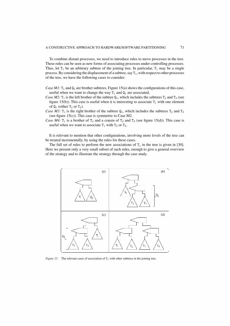
To combine distant processes, we need to introduce rules to move processes in the tree.These rules can be seen as new forms of associating processes under controlling processes.Thus, let T1 be an arbitrary subtree of the joining tree. In particular, T1 may be a singleprocess. By considering the displacement of a subtree, say T1, with respect to other processesof the tree, we have the following cases to consider:

Case M1: T1 and Q1 are brother subtrees. Figure 15(a) shows the configurations of this case,useful when we want to change the way T1 and Q1 are associated.

Case M2: T1 is the left brother of the subtree Q1, which includes the subtrees T2 and T3 (seefigure 15(b)). This case is useful when it is interesting to associate T1 with one elementof Q1 (either T2 or T3).

Case M3: T1 is the right brother of the subtree Q1, which includes the subtrees T2 and T3(see figure 15(c)). This case is symmetric to Case M2.

Case M4: T1 is a brother of T2 and a cousin of T3 and T4 (see figure 15(d)). This case isuseful when we want to associate T1 with T3 or T4.

It is relevant to mention that other configurations, involving more levels of the tree canbe treated incrementally, by using the rules for these cases.

The full set of rules to perform the new associations of T1 in the tree is given in [30].Here we present only a very small subset of such rules, enough to give a general overviewof the strategy and to illustrate the strategy through the case study.

Figure 15. The relevant cases of association of T1 with other subtrees in the joining tree.


The rules of Case M1 are similar to the ones of brother processes and we omit an ex-ample here. In Cases M2 and M3, we need to introduce rules for the situation in whichthe controlling processes involved are: both sequential, both parallel and mixed (one par-allel and the other one sequential). Moreover, we need to introduce rules to associate T1with T2 and also T1 with T3. Here we will give only two of the rules applied in thesecases.

Rule 6.4 (PAR-PAR-1) is of Case M2. This rule is used to associate subtrees T1 andT2 as brother subtrees and is directly derived from the associativity of the paralleloperator.

Rule 6.4 (PAR-PAR-1).

Figure 16.

Rule 6.5 (SEQ-PAR-3) is of Case M3, when mixed controlling processes are involved.This rule is also used to associate the subtrees T1 and T2 as brothers subtrees. Neverthe-less, in this case the execution of either the subtrees T2 and T3 or T1 and T3 changes.Thus, this rule has two cases. In Case A, the configuration on the left-hand side of therule is transformed into the configuration of the right-hand side of the rule, if T2 is inde-pendent of T3 and the environment offers the possibility to synchronise the channels ofT3 before synchronising with any channel of T2. The transformation expressed by CaseB is possible when T1 is independent of T3 and the environment offers the possibilityto synchronise the channels of T3 before synchronising with any channel of T1. More-over, in Case B, the local variables of the sequential controlling process is now the lo-cal variable of the parallel controlling process. The transformations expressed by theserules involve basically a rearrangement of the communication inside the controlling pro-cesses shown and, in Case A, the parallel controlling process is replaced by a sequentialone.


Rule 6.5 (SEQ-PAR-3).

Figure 17.

In Case M4, the relevant configurations to consider are the ones whose external controllingprocess is different from the internal ones. The other cases may be reduced to cases M2and M3. One rule applied in Case M4 is Rule 6.6 (PAR-SEQ-SEQ-1), which associates T1with T3 and, as a consequence, T2 with T4. It can be applied if T1 is independent of T4, T2is independent of T3, the environment offers the possibility to synchronise the channels ofT1 (T3) before synchronising with any channel of T4 (T2).

The rules to approximate and combine processes are applied to all pair of processes insidea PARpar or PARser construct. If all these processes are combined, the construct will beunitary. By applying Law 2.11 (PARser unit) and a similar one for the PARpar construct,the combined process is considered as a new process of the immediate upper level of thedescription hierarchy. Nevertheless, it may be the case that the approximation procedurestops, in order to avoid that the semantics of the description be violated. In this case, theconstruct is not completely reduced and its remaining processes are not considered on thecomposition of the pairs, when the immediate upper PARpar or PARser construct is analisedduring the first stage. Only combined processes or processes derived from the splitting phaseare considered on the composition of the pairs. When, after the first stage, some PARpar orPARser constructs remain unreduced, the second stage of the combination procedure takesplace, with the aim of guaranteeing that the final description will follow what is required bythe phase of definition of components. In this stage, the way of execution of the processesbelonging to different levels of the component hierarchy is analysed and eventually some


additional movement of processes in the tree is performed, by using the rules for casesM1 and M2. The characteristic of such transformations is that the communication is noteliminated, as processes are not effectively combined in the second stage; at most thecommunication among them is rearranged in a convenient form.

Rule 6.6 (PAR-SEQ-SEQ-1).

Figure 18.

The description of the components is a byproduct of the rules applied in the first and(eventually) in the second stages. In the third stage, to generate the interface process bycombining controlling processes, it is necessary to introduce rules to eliminate the commu-nication among them. We need to deal with the case in which a sequential and a parallelcontrolling processes are involved. Here we show the rule to solve the former case and werefer to the rule for the latter case as Rule par. communication elim.

The aim of Rule 6.7 (seq. communication elim.) is to eliminate the communication throughchannels ch1 and ch2. Observe that no additional transformation is performed and the orderof execution of the processes involved is the same, on both sides of the rule. The role ofthe processes P1 and P3 is to allow the use of the same rule to eliminate the left and theright communication of sequential controlling processes. In the former case, P1 is SKIPand, in the latter case, P3 is SKIP. The controlling process may include communicationwith the environment, depending on whether it is the root of the joining tree. This possiblecommunication is expressed by processes Q1 and Q2. If the controlling process is the rootof the joining tree, Q1 and Q2 are SKIP. Otherwise, if the controlling process is an internalnode of the tree, Q1 has the form ch?x and Q2 has the form ch’!x’, where ch and ch’ arechannels introduced by the splitting phase. The role of process T1 is to express the otherpossible processes of the PAR construct. Observe that this rule does not include the CONconstructor. We assume that Law 2.10 (CON unit) is applied before this rule.

Rule 6.7 (seq. communication elim.).

PAR

VAR x2, z2 : SEQ(ch1 ? x2, z2, P2, ch2 ! x′2, z′

2)

VAR x : SEQ(Q1, VAR z : SEQ(P1, SEQ(ch1!x2, z2, ch2?x′2, z

′2), P3), Q2)

T1


=PAR(VAR x : SEQ(Q1, VAR z : SEQ(P1, P2, P3), Q2), T1)

provided free(P2) = x2 ∪ z2, free(P1) ⊆ (x ∪ z), free(P3) ⊆ (x ∪ z),

free(Q1) ⊆ x and free(Q2) ⊆ x.

As mentioned before, the strategy can fail, in the case a transformation, required by thephase of definition of components, violates the semantics of the original description ofthe system. Thus, we need to introduce rules to deal with such failure situations. Rule 6.8(fail-1) is one of these rules and expresses the fact that two sequential brother processescannot be combined in parallel, if they are data-dependent.

Rule 6.8 ( fail-1).

PARpar

PAR

VAR x1, z1 : SEQ(ch1 ? x1,z1, P1, ch2 ! x′1,z

′1)


′2)

VAR x: CON(SEQ(Q1, VAR z: SEQ(SEQ(ch1 ! x1,z1, ch2 ?x′1,z

′1),

SEQ(ch3 ! x2,z2, ch4 ? x′2,z

′2)), Q2))

T1=PARpar(VAR x : SEQ(Q1, PARparFail(VAR z : SEQ(P1, P2)), Q2), T1)

provided free(P1) = x1 ∪ z1, free(P2) = x2 ∪ z2, free(Q1) ⊆ x,

free(Q2) ⊆ x and dependency((x1, z1), (x′1, z

′1), (x2, z2), (x′

2, z′2)).

The boolean function dependency returns TRUE if the following condition is satisfied(P1 and P2 have data-dependency),

(x1 ∪ z1) ∩ (x′2 ∪ z′

2) �= {} ∨ (x2 ∪ z2) ∩ (x′1 ∪ z′

1) �= {}

otherwise, the function returns FALSE.If two processes of a given component cannot be combined as required by the phase of

definition of components, it does not make sense to continue the application of the joiningstrategy to combine processes in a higher level of this component hierarchy. In a later stageof the design flow the description of this component should be revised by the designer.Thus, we have also rules to propagate the failure of an internal PARpar or PARser constructto the higher levels of the component hierarchy (see [30, Chap. 5]).

To illustrate the application of the strategy of combining processes, consider processes Q3to Q15 of figure 10. Recall that the description of each Qi includes the process Pi (depictedin the tree of the same figure) inserted into a replicated context and the communicationintroduced by the splitting phase (represented by the edges of the tree). We focus on thetransformations which do not involve the replicated structures and we assume that the


Figure 19. Combining brother processes of the case study.

replicated construct is part of the context into which these transformations are applied.Thus, we show transformations in the subtree included into the thick big box of figure 10.

By considering the description generated by the phase of definition of components, firstlythe joining strategy combines all brother processes belonging to a same PARpar or PARserconstruct, starting from the most internal level of the component descriptions to the externalone. Thus, the first transformation performed is the combination of processes Q14 and Q15,by applying the rule to solve Case B2, which basically eliminates the controlling process.After this transformation, each component includes only onePARser construct. The strategyproceeds by combining the brother processes of the PARser constructs. Then, process Q13is combined with process Q14‖15, and process Q10 is combined with process Q11, as shownin figure 19 (compare with figure 10). Both transformations use Rule 6.2 (SEQ-1). (Thesymbols ; and ‖ stand for sequential and parallel composition.)

The combination of Q10 and Q11 generates another pair of brother processes, formed by Q9and Q10;11. Thus, again Rule 6.2 (SEQ-1) is applied to reduce this new pair. This procedureis repeated until the tree meets the configuration depicted in figure 20.


Figure 20. Additional combination of the brother processes of the case study.

Notice that all brother processes belonging to the same PARser construct have beencombined; thus, we proceed by combining distant processes. So, processes Q3 and Q4 in thesoftware component are approximated, as well as the processes of the hardware component.These processes are in the same level of the description hierarchy; Q3 and Q4 are structuredas in Case A1, whereas the processes of the hardware component are structured as in CaseA2. Rule 6.4 (PAR-PAR-1) is applied to approximate processes Q3 and Q4, resulting in theconfiguration of figure 21(a).

After that, these processes are combined by applying Rule 6.3 (PAR-2) and the seri-alisation strategy, briefly described in Section 6.4 (see figure 21(b)). Then, Case A ofRule 6.5 (SEQ-PAR-3) is applied to approximated the processes of the hardware compo-nent (see figure 21(c)). Next, these processes are combined by applying Rule 6.2 (SEQ-1)(see figure 21(d)). Due to the replicated structure and data-dependency among processes,the combination procedure of the first step stops.

As all processes are executing as required by the phase of definition of components, atsecond stage no additional transformations are necessary. Then, the strategy proceeds bygenerating the interface process. Rule 6.7 (seq. communication elim.) is used to eliminateall communication among controlling processes, resulting the description of figure 22.

6.2. Step J2: Reconstructing IF and ALT commands

If the reconstruction of IF and ALT commands are total, in the sense that all original branchesare put together after partitioning, the splitting rules of Step 1 can be applied in this case.Nevertheless, if some branches of these constructs are spread into distinct components, weneed to introduce rules to partially reconstruct such commands. For conciseness reasons


Figure 21. Additional transformations of the example of figure 19.

we omit these rules (see [30] for details). The third conditional of the original example (seefigure 3(a)), fragmented during the splitting phase is reconstructed by applying the sameset of rules of the splitting phase (from right to left), as all branches belong to the hardwarecomponent; to see this transformation, compare the form of the conditionals (in the hardwarecomponent) in figure 4 (which represents the final result of the partitioning) and 22.

6.3. Step J3: Performing some optimisations

This step performs some optimisations in the description of the partitioned system with theaim of eliminating unnecessary variables and communication between the interface process


Figure 22. The description of the case study generated after the step of combining processes.

and some components. For example, Rule 6.9 (otim-1) is applied in the following situation:two sequential processesP1 andP2 of a same component receive the variabley from the inter-face process, and the interface process does not receivey from any other process that executesbetween P1 and P2. In this case, only P1 needs to receive y. Nevertheless, both processes maysend y (if y is assigned in these processes), as this variable may be used by another processthat executes between P1 and P2. In the description of this rule, a higher-order function Fis used to abstract the context of the interface process, making explicit only the channels ofthis process, in the textual order they appear. The higher-order functions H and I abstract thecontext in which P1 and P2 are immersed. The term T1 represents all the other components.

Rule 6.9 (otim-1).

CHAN ch1, ch′1, ch2, ch′

2, . . . , chm, ch′m :

PAR

VAR x: CON(F(ch1 ! x1, ch′1 ? x′

1, . . . , chi ! xi, y, ch′i ? x′

i, y, . . . ,

chj ! xj, y, ch′j ? x′

j, y, . . . , chm ! xm, ch′m ? x′

m))

H(SEQ(VAR xi, y : SEQ(chi ? xi, y, P1, ch′i ! x′

i, y),

I(VAR xj, y : SEQ(chj ? xj, y, P2, ch′j ! x′

j, y))))

T1


=CHAN ch1, ch′

1, ch2, ch′2, . . . , chm, ch′

m :

PAR

VAR x: CON(F(ch1 ! x1, ch′1 ? x′

1, . . . , chi ! xi, y, ch′i ? x′

i, . . . ,

chj ! xj, ch′j ? x′

j, y, . . . , chm ! xm, ch′m ? x′

m))

H(VAR y:SEQ(VAR xi : SEQ(chi ? xi, y, P1, ch′i ! x′

i),

I(VAR xj : SEQ(chj ? xj, P2, ch′j ! x′

j, y))))

T1

provided all bound variables of the first process have

distinct names and y does not appear in any xk, i < k < j.

For example, this rule is used to eliminate the passage of variables aux, b, e, w andy through channel spch3 of the description of figure 22. By applying some optimisationrules, and some laws of occam to linearise the description, the example achieves the formgiven in figure 4.

6.4. The serialisation strategy

A very important part of the joining strategy is a strategy to serialise parallel processes.This strategy is fully described in [30, 31]. Basically, if Rule 6.1 (Serialisation-1) cannotbe applied, the serialisation of P1 and P2 is performed gradually, by analysing each of theirsubprocesses. For example, figure 23 shows a simple example of a gradual serialisation ofprocesses Pu and Pv, where the environment is represented by process Pz. Observe that as thechannels of Pu and Pv synchronise in an interleaved way with Pz, Rule 6.1 (Serialisation-1) cannot be applied (either the restriction PuPv or PvPu is violated). Nevertheless, wecan perform the serialisation of Pu and Pv by exhaustively serialising their subprocesses,according to the order of execution of the channels in Pz, as shown in figure 23(b) and (c).

To perform the gradual serialisation some laws of occam and Lemma 6.1 (PAR-SEQresult) (and some results derived from it) are applied. This lemma is a generalisation of asimilar result for disjoint processes presented in [14, Chap. 7].

Lemma 6.1 (PAR-SEQ result).

PAR(SEQ(Q1, Q2), SEQ(T1, T2)) =(E,(Q1T2,T1Q2)) SEQ(PAR(Q1, T1), PAR(Q2, T2))

Figure 23. An example of a gradual serialisation of Pu and Pv.


As processes P3 and P4 of figure 3 have no communication command and they are dataindependent, Rule 6.1 (Serialisation 1) is applied to perform the serialisation.

7. Implementation

The basic laws of occam, the splitting rules and some of the joining rules can be easilyencoded as rewrite rules (in a term rewriting system) or as functions in a functional pro-gramming language. Nevertheless, the majority of the joining rules are applied only if theenvironment offers the possibility of respecting the order of synchronisation of the listof restriction S. Thus, when implementing these rules, we need to provide an automaticmechanism to capture the environment, and to identify the order of execution of events.

As the splitting normal form is a set of parallel processes, to capture the environment E,when the joining rules are applied, we basically apply Law 2.4 (PAR assoc). The environmentis formed by all processes not included into the subtree, whose root is the first commonancestor of the processes to combine. For example, figure 24 shows the environment of Pxand Py, when these processes are approximated.

To identify the order of execution of events a simple possibility is to derive a directedgraph from the environment description, called here sequence graph, defined in the sequel.

Definition 7.1 (Sequence graph). Let P be a deadlock-free occam process allowing onlyone point of synchronisation. The sequence graph of P, denoted by GS(P) is a directedgraph whose set of vertices is the set of channel variables of P. Two vertices ch1 and ch2in GS(P) are connected by a directed path from ch1 to ch2 if and only if ch1 synchronisesbefore ch2 in P.

Thus, to identify if restriction PxPy is satisfied by the environment E, it is enough togenerate GS(E) and to check the following condition:

∀ chi ∈ Px, chj ∈ Py . not(path(chj, chi, GS(E)))

Figure 24. An example of how to capture the environment when joining rules are applied.


where path is a function which returns TRUE if there exists a path from chj to chi inGS(E); otherwise, it returns FALSE. This function may be implemented by using the classicdepth-first search algorithm, by taking chj as the root of the search. The algorithm to deriveGS of a process P is given in [30], as well as a proof of its correctness.

8. The ParTS tool

To carry out the partitioning verification automatically, a tool, the Partitioning Transforma-tion System (ParTS), has been developed [18, 19]. This tool has been implemented as anextension of the occam Transformation System (OTS) [10], which performs general trans-formations of occam programs. While the basic laws of occam [25] implemented in OTSare useful for program transformation in general, they are not suitable to capture the parti-tioning problem. ParTS extends OTS with the implementation of the splitting, joining andserialisation rules, as well as the strategies which guide the application of these rules. Eachtransformation rule is captured in ParTS by a function in the SML [12] language. The strate-gies are also coded as functions, taking advantage of the pattern matching facilities of SML.

Figure 25 shows the interface of ParTS, which is implemented in Java [8] and allows usersto manipulate several occam processes in different windows. Moreover, the portability ofJava allows one to use the same version of ParTS on different platforms. The tool provides a

Figure 25. The ParTS interface.


file menu (including open and save options), zoom facilities and a combo box which allowsthe user to select a law or a rule to be applied to the current process. It contains rules namedas split and join which perform the transformations to carry out the hardware/softwarepartitioning.

9. Conclusions

This paper presents an innovative approach to hardware/software partitioning, with em-phasis on correctness. We characterise partitioning as a program transformation task, andpropose a partitioning methodology comprising three main phases: splitting, definition ofcomponents and joining. The main contribution of this paper is a formal strategy to carryout the splitting and joining phases automatically in a constructive way.

There are some key points addressed by this work which do not seem to have been exploredin the literature. One of them is uniformity: the specification and reasoning mechanism isthe same, the occam language. In all approaches to partitioning mentioned in Section 1, thespecification language is distinct from the internal model in which the system is represented.The semantic gap between language and model makes the verification of the partitionedsystem an extremely difficult task. Moreover, the fact that the output of the partitioning isstill an occam program may be very useful to carry out simulation in a very early stage ofthe co-design flow, without the need of any translation.

Although we have used occam all the way through the partitioning process, this workcould be adapted, so that occam is used only as an internal model. However, in this casea translation from the specification language into occam (and/or from occam to the targetlanguage) would be required. Ideally, such translations should be provably correct, forobvious reasons.

Another important point to single out is the orthogonality between functional and non-functional issues of the partitioning. This means that the program transformation phaseswhich guarantees the correctness of the functional behaviour (splitting and joining) may beused in conjunction with several published heuristics to partitioning provided, of course, thatthe description language is the subset of occam considered here and the interfaces amongthe partitioning phases are respected. More than that, the splitting and joining phases areindependent of the evolution of partitioning algorithms, and this is a trend, as co-designmethodologies are all in an initial stage.

Furthermore, our approach to verification is absolutely independent of the target architec-ture in which the system will be implemented. The majority of the partitioning approachesconsiders only one software component and several hardware ones. Nevertheless, it is atrend in co-design to enlarge the number of software components considered. The correct-ness phases deal with hardware and software components indistinctly: they are just occamprocesses. Thus, the number of such components is irrelevant for the verification task.

As a byproduct of the strategy proposed, the interface process is generated automatically.As mentioned before, this process includes the communication among hardware and soft-ware components. The explicit generation of this communication makes easier and less errorprone the interface synthesis task. In all approaches mentioned in Section 1, the generationof the interface process is not carried out automatically.


Our approach provides full flexibility of exploring the design space, as well as allowinguser interaction. In the splitting and joining phases the former characteristic is related tothe fact that the normal form of the splitting phase is a set of parallel processes. Since par-allelism in occam is associative and commutative, this form allows the designer to analyseany permutation of processes, when grouping them in components. The latter characteristicis related to the introduction of the BOX constructor. By using this constructor, the designercan interfere in the granularity of the original processes to be analysed by the partitioning al-gorithm. As the granularity of processes considered by the several heuristics to partitioningvaries from fine (primitive commands) to coarse (chunks of code), this constructor is spe-cially useful to allow the use of the correctness phases in conjunction with these heuristics.

Moreover, the proposed rules for partitioning do not incorporate any co-design particu-larity. Thus, we believe that they could be used in other contexts.

Most importantly, what we consider the main contribution of this work is its originality. Asmentioned before, we are not aware of any other approach which formalises the partitioningproblem as a program transformation task as we have done here. Few approaches (POLIS[15] and LAMBDA [16]) use formal methods to validate the partitioning. The TOSCA co-design system [1] suggests the use of some user-driven occam laws to prove the correctnessof some transformations. Nevertheless, none of them develop a formal strategy to ensurethat the partitioning preserves the functionality of the original description.

By using the ParTS tool briefly described in Section 8, some small case studies havebeen developed, among them the convolution program (here illustrated), an ATM controllerswitch [19] and an intravenous infusion control system [5]. In the first example, the hard-ware/software mixed implementation achieves the time constraints and have an area cost53% smaller than a hardware implementation. For the infusion controller system, a mixedimplementation has reduced drastically the setup time: 54 ns for a software implementationagainst 15,2 ns for a hardware/software mixed implementation. To develop medium andlarge case studies is the immediate task of the PISH team.

As mentioned in Section 2, the strategy presented here was extended to consider repli-cators in all constructs of the occam grammar, given in that section, enlarging in this waythe expressiveness of the subset of occam adopted. The next step is to extend the strategyto consider functions, procedures and arbitrary loops (as we have considered only fixediteration).

Appendix A: Proving Rule 6.6 (PAR-SEQ-SEQ-1)

To illustrate how the hardware/software partitioning in the style suggested in this workmay be proved to be a semantic-preserving transformation process, we prove Rule 6.6(PAR-SEQ-SEQ-1). By chosing this rule, we also illustrate that the occam version of thejoining rules can be straightforwardly derived from the diagrammatic version of such rules,as shown in the sequel. The role of processes Q1 and Q2 is the same as mentioned in Rule 6.7(seq. communication elim.). In the occam version the subtrees T1 to T4 may be representedby a process derived from the original description of the system (if the subtree is unitary) orby the controlling process which is the root of the subtree (when the subtree includes morethan one process). The role of function H is to abstract the CON construct, if this is the case.


Rule 6.6 (PAR-SEQ-SEQ-1).

PAR

VAR x11, z1 : H(SEQ(ch5 ? x11,z1, P1, ch6 ! x′1,z

′1))

VAR x12, z2 : H(SEQ(ch7 ? x12,z2, P2, ch8 ! x1 ′2,z

′2))

VAR x21, t1 : H(SEQ(ch9 ? x21,t1, P3, ch10 ! x2 ′1,t

′1))


′2))

VAR x1 : CON(SEQ(ch1 ? x1,

VAR z: SEQ(SEQ(ch5 ! x11,z1, ch6 ? x1 ′1,z

′1),

SEQ(ch7 ! x12,z2, ch8 ? x1 ′2,z

′2)),

ch2 ! x′1))

VAR x2 : CON(SEQ(ch3 ? x2,

VAR t: SEQ(SEQ(ch9 ! x21,t1, ch10 ? x2 ′1,t

′1),

SEQ(ch11 ! x22,t2, ch12 ? x2 ′2,t

′2)),

ch4 ! x′2))

VAR x: CON(SEQ(Q1,PAR(SEQ(ch1 ! x1, ch2 ? x′1),

SEQ(ch3 ! x2, ch4 ? x′2)),Q2))

=(E,P1P4,P2P3)

PAR

VAR x11, z1 : H(SEQ(ch5 ? x11,z1, P1, ch6 ! x′1,z

′1))

VAR x12, z2 : H(SEQ(ch7 ? x12,z2, P2, ch8 ! x1 ′2,z

′2))


′1))


′2))

VAR x11, z1,x21, t1 :

CON(SEQ(ch1 ? x11,z1,x21,t1,

PAR(SEQ(ch5 ! x11, z11, ch6 ? x1 ′1, z1

′1),

SEQ(ch9 ! x21,t1, ch10 ? x2 ′1,t

′1)),

ch2 ! x′1,z

′1,x2

′1,t

′1))

VAR x12, z2, x22, t2 :

CON(SEQ(ch3 ? x2,z2,x22,t2,

PAR(SEQ(ch7 ! x12,z2, ch8 ? x1 ′2,z

′2),

SEQ(ch11 ! x22,t2, ch12 ? x2 ′2,t

′2)),

ch4 ! x′2,z

′2,x2

′2,t

′2))

VAR x: CON(SEQ(Q1,VAR z, t:

SEQ(SEQ(ch1 ! x11,z1,x21,t1, ch2 ? x′1,z

′1,x2

′1,t

′1),

SEQ(ch3 ! x12,z2,x22,t2, ch4 ? x1 ′2,z

′2,x2

′2,t

′2)),

Q2))

provided free(P1) = x11 ∪ z1, free(P2) = x12 ∪ z2,

free(P3) = x21 ∪ t1, free(P4) = x22 ∪ t2,


free(Qi) ⊆ x,i = 1,2,

not(dependency((x11, z11), (x1 ′1,z

′1), (x22,t2), (x2 ′

2,t′2))),

not(dependency((x12,z2), (x1 ′2,z

′2), (x21,t2), (x2 ′

1,t′2))).

Proof:LHS

= {Laws 2.10 (CON unit), 2.4 (PAR assoc) 2.5 (PAR sym),

2.2 (SEQ assoc), 2.1 (SEQ-SKIP unit)}PAR


′1)

VAR x1 : SEQ(ch1 ? x1,

VAR z: SEQ(SKIP, SEQ(ch5 ! x11,z1, ch6 ? x1 ′1,z

′1),

SEQ(ch7 ! x12,z2, ch8 ? x1 ′2,z

′2)),

ch2 ! x′1)

PAR

VAR x12, z2 : SEQ(ch7 ? x12,z2, P2, ch8 ! x1 ′2,z

′2)

PAR

VAR x21, t1 : SEQ(ch9 ? x21,t1, P3, ch10 ! x2 ′1,t

′1)


VAR t: SEQ(SKIP,

SEQ(ch9 ! x21,t1, ch10 ? x2 ′1,t

′1),

SEQ(ch11 ! x22,t2, ch12 ? x2 ′2,t

′2)),

ch4 ! x′2)

PAR

VAR x22,t2 : SEQ(ch11 ? x22,t2, P4, ch12 ! x2 ′2,t

′2)

VAR x:SEQ(Q1,PAR(SEQ(ch1 ! x1, ch2 ? x′1),

SEQ(ch3 ! x2, ch4 ? x′2)),Q2)

= {Rule 6.7 (seq. communication elim.)}PAR


VAR z: SEQ(SKIP, P1,

SEQ(ch7 ! x12,z2, ch8 ? x1 ′2,z

′2)),

ch2 ! x′1)

PAR


′2)

PAR


VAR t: SEQ(SKIP, P3,

SEQ(ch11 ! x22,t2, ch12 ? x2 ′2,t

′2)),

ch4 ! x′2)


PAR

VAR x22,t2 : SEQ(ch11 ? x22,t2, P4, ch12 ! x2 ′2,t

′2)


SEQ(ch3 ! x2, ch4 ? x′2)),Q2)

= {Laws 2.4 (PAR assoc) 2.5 (PAR sym)}

PAR


′2)


VAR z: SEQ(SKIP, P1,

SEQ(ch7 ! x12,z2, ch8 ? x1 ′2,z

′2)),

ch2 ! x′1)

PAR

VAR x22,t2 : SE Q(ch11 ? x22,t2, P4, ch12 ! x2 ′2,t

′2)


VAR t: SEQ(SKIP, P3,

SEQ(ch11 ! x22,t2, ch12 ? x2 ′2,t

′2)),

ch4 ! x′2)


SEQ(ch3 ! x2, ch4 ? x′2)),Q2)

= {Laws 2.2 (SEQ assoc), 2.1 (SEQ − SKIP unit)

and Rule 6.7 (seq. communication elim.)}PAR


VAR z: SEQ(P1, P2, SKIP),

ch2 ! x′1)

PAR


VAR t: SEQ(P3, P4, SKIP)

ch4 ! x′2)


SEQ(ch3 ! x2, ch4 ? x′2)),Q2)

= {Laws 2.1 (SEQ–SKIP unit), 2.2 (SEQ assoc)

2.3 (PAR–SKIP unit), 2.4 (PAR assoc)

2.5 (PAR sym) and Rule (par. communication elim.)}PAR


VAR z: SEQ(P1, P2),ch2 ! x′

1)



VAR t: SEQ(P3, P4)),Q2)

SKIP

= {Rule (par. communication elim.)}VAR x: SEQ(Q1, PAR(VAR z: SEQ(P1, P2),

VAR t: SEQ(P3, P4)), Q2)

= {Laws 2.8 (VAR − PAR), 2.5 (PAR sym)

and 2.7 (VAR assoc)}VAR x: SEQ(Q1,VAR z,t:PAR(SEQ(P1,P2),SEQ(P3,P4)), Q2)

=(E,P1P4,P2P3) {Lemma 6.1 (PAR–SEQ result)}VAR x: SEQ(Q1, VAR z,t : SEQ(PAR(P1,P3), SEQ(P2,P4)), Q2)

= {Laws 2.2 (SEQ assoc), 2.1 (SEQ–SKIP unit),

2.3 (PAR–SKIP unit), rules par. communication elim.,

6.7 (seq. communication elim.) and Laws 2.4 (PAR assoc)

2.5 (PAR sym) and 2.10 (CON unit)}RHS

In general, in all proofs of the joining rules the communication of the left-hand side isfirst eliminated using rules (par. communication elim.) and 6.7 (seq. communication elim.).After that, Lemma 6.1 (PAR-SEQ result) is applied or some results derived from this lemma.Finally, Rules (par. communication elim.) and 6.7 (seq. communication elim.) are againapplied to reconstruct the communication of the right-hand side of the rule. Additionally,Law 2.10 (CON unit) is used to eliminate (and after to introduce) the CON constructor andLaws 2.4 (PAR assoc) and 2.5 (PAR sym) are used to rearrange, in a convenient form, theparallel processes before and after the main transformation.

Acknowledgments

The authors acknowledge Juliano Iyoda, He Jifeng, Geraint Jones, George Justo, AnaCavalcanti and Paulo Borba for discussing this work and making some valuable suggestions.We also would to thank the anonymous referees for the very datailed and useful comments.The authors also acknowledge the financial support given by the Brazilian research agencies,CNPq and CAPES.

References

1. A. Balboni, W. Fornaccari, and D. Sciuto, “TOSCA: A pragmatic approach to co-design automation of control-dominated systems,” in Hardware/Software Co-design, Kluwer Academic Publisher, 1996, pp. 265–294.

2. E. Barros, Hardware/Software Partitioning Using UNITY. PhD thesis, Tubingen University, 1993.3. E. Barros and A. Sampaio, “Towards probably correct hardware/software partitioning using occam,” in Pro-

ceedings of the Third International Workshop on Hardware/Software Co-Design CODES/CASHE94, IEEEPress, 1994, pp. 210–217.


4. E. Barros, A. Sampaio, M.E. Lima, L. Silva, R. Jacobi, and N. Calazans, “The PISH methodology forhardware/software co-design,” in Workshop of ProTem-CC, CNPq, 1998, pp. 65–98.

5. E. Barros and M.V.D. Santos, “A safe, accurate intravenous infusion control system,” IEEE Micro Magazine,1998.

6. K.V. Berkel, J. Kessels, M. Ronchin, R. Saeijs, and F. Schalij, “The VLSI-programming language tangram andits translation into handshake circuits,” in Proceedings of the European Conference on Design Automation,1991, pp. 384–391.

7. R. Bird, Introduction to Functional Programming Using Haskell, Prentice Hall, 1998.8. M. Campione and K. Walrath, The Java Tutorial: Oject-Oriented Programming for Internet, Addison-Wesley,

1998.9. R. Ernst and J. Henkel, “Hardware-software co-design of embedded controllers based on hardware extraction,”

in Handouts of the International Workshop on Hardware-Software Co-Design, 1992.10. M. Goldsmith, The Oxford occam Transformation System. Technical report, Oxford University Computing

Laboratory, Jan. 1988.11. R. Gupta and G. De Micheli, “System-level synthesis using re-programmable components,” in Proceedings

of EDAC, IEEE Press, 1992, pp. 2–7.12. R. Harper, D. MacQueen, and R. Milner, Standard ML. Edinburgh University LFCS report series ECS-LFCS-

86-2, 1986.13. J. He, I. Page, and J. Bowen, “A provable hardware implementation of occam,” Correct Hardware Design

and Verification Methods (Advanced Research Working Conference, CHARME’ 93), Vol. 693, Lecture Notesin Computer Science, Springer Verlag, 1993, pp. 214–225.

14. C.A.R Hoare and J. He, Unifying Theories of Programming, Prentice-Hall, 1998.15. H. Hsieh, A. Sangiovanni-Vicentelli, F. Ballarin, and L. Lavagno, “Synchronous equivalence for embedded

systems: A tool for design exploration,” in Proceedings of the International Conference on Computer-AidedDesign, 1999, pp. 505–509.

16. R.B. Hughes and G. Musgrave, “The lambda approach to system verification,” in Hardware/Software Coo-design, Kluwer Academic Publisher, 1996, pp. 427–451.

17. Institute of Electrical and Electronics Engineers, New York, USA, IEEE Standard VHDL Language ReferenceManual (IEEE Std 1076-1987), 1987.

18. J. Iyoda, A. Sampaio, and L. Silva, “ParTS: A partitioning transformation system,” in Proceedings of FM99(World Congress on Formal Methods), Vol. 1709, Lecture Notes in Computer Science, 1999, pp. 1400–1419.

19. J. Iyoda, ParTS: A Support Tool to Hardware/Software Partitioning. Master thesis, Federal University ofPernambuco, Brazil, May 2000 (in Portuguese).

20. G. Jones and M. Goldsmith, Programming in Occam 2, Prentice-Hall, 1988.21. A. Kalavade and E. Lee, “The extended partitioning problem: Hardware/software mapping, scheduling and

implementation-bin selection,” Design Automation for Embedded Systems, Vol. 2, No. 2, pp. 125–163, 1997.22. C. Kern and M. Greenstreet, “Formal verification in hardware design: A survey,” ACM Transactions in Design

Automation of Electronic Systems, Vol. 4, No. 2, pp. 123–193, 1999.23. J. Madsen, J. Groge, P.V. Knudsen, M.E. Petersen, and A. Haxthausen, “Lycos: The lyngby co-synthesis

system,” Design Automation of Embedded Systems, Vol. 2, No. 2, pp. 195–235, 1997.24. R. Niemann and P. Marwedel, “An algorithm for hardware/software partitioning using mixed integer linear

programming,” Design Automation of Embedded Systems, Vol. 2, No. 2, pp. 165–193, 1997.25. A.W. Roscoe and C.A.R. Hoare, “The laws of occam programming,” Theoretical Computer Science, Vol. 60,

pp. 177–229, 1988.26. D. Saha, R.S. Mitra, and A. Basu, “Hardware/software partitioning using genetic algorithm,” in Proc. of 10th

International Conference on VLSI Design, India, 1997, pp. 155–160.27. A. Sampaio, An Algebraic Approach to Compiler Design. Vol. 4 of Algebraic Methodology and Software

Technology (AMAST) Series in Computing, World Scientific, 1997.28. L. Silva, A. Sampaio, and E. Barros, “A normal form reduction strategy for hardware/software partitioning,”

in Formal Methods Europe (FME) 97. Vol. 1313, Lecture Notes in Computer Science, 1997, pp. 624–643.29. L. Silva, A. Sampaio, E. Barros, and J. Iyoda, “An algebraic approach to combining processes in a hard-

ware/software partitioning environment,” in 7th International Conference on Algebraic Methodology andSoftware Technology (AMAST) 98, Vol. 1548, Lecture Notes in Computer Science, 1999, pp. 308–324.


30. L. Silva, An Algebraic Approach Hardware/Software Partitioning. PhD. thesis, Federal University of Pernam-buco, Recife, Brazil, July 2000.

31. L. Silva, A. Sampaio, and G. Jones, “Serialising parallel processes in a hardware/software partitioning context,”in Proceedings of Formal Method Europe (FME) 2001, Vol. 2021, Lecture Notes in Computer Science, 2001,pp. 344–363.

32. W. Wu, I. Sader, and A. Jantsch, “Transformational system design based on a formal computational modeland skeletons,” in Proceedings of the Forum on Design Languages, 2000.

A Constructive Approach to Hardware/Software Partitioning

Documents

Transcript of A Constructive Approach to Hardware/Software Partitioning