Huang et al. Geothermal Energy (2015) 3:13 DOI 10.1186/s40517-015-0030-8

RESEARCH Open Access

Extending the persistent primary variablealgorithm to simulate non-isothermaltwo-phase two-component flow with phasechange phenomenaYonghui Huang1,2†, Olaf Kolditz1,2 and Haibing Shao1,3*†

*Correspondence:haibing.shao@ufz.de†Equal contributors1Helmholtz Centre forEnvironmental Research - UFZ,Permoserstr. 15, 04318 Leipzig,Germany3Freiberg University of Mining andTechnology, Gustav-Zeuner-Strasse1, 09596 Freiberg, GermanyFull list of author information isavailable at the end of the article

Abstract

In high-enthalpy geothermal reservoirs and many other geo-technical applications,coupled non-isothermal multiphase flow is considered to be the underlying governingprocess that controls the system behavior. Under the high temperature and highpressure environment, the phase change phenomena such as evaporation andcondensation have a great impact on the heat distribution, as well as the pattern offluid flow. In this work, we have extended the persistent primary variable algorithmproposed by (Marchand et al. Comput Geosci 17(2):431–442) to the non-isothermalconditions. The extended method has been implemented into the OpenGeoSys code,which allows the numerical simulation of multiphase flow processes with phasechange phenomena. This new feature has been verified by two benchmark cases. Thefirst one simulates the isothermal migration of H2 through the bentonite formation in awaste repository. The second one models the non-isothermal multiphase flow ofheat-pipe problem. The OpenGeoSys simulation results have been successfully verifiedby closely fitting results from other codes and also against analytical solution.

Keywords: Non-isothermal multiphase flow; Geothermal reservoir modeling;Phase change; OpenGeoSys

BackgroundIn deep geothermal reservoirs, surface water seepages through fractures in the rockand moves downwards. At a certain depth, under the high temperature and pressurecondition, water vaporizes from liquid to gas phase. Driven by the density difference, thegas steam then migrates upwards. Along with its path, it will condensate back into theliquid form and release its energy in the form of latent heat. Often, this multiphase flowprocess with phase transition controls the heat convection in deep geothermal reservoirs.Besides, suchmultiphase flow and heat transport are considered to be the underlying pro-cesses in a wide variety of applications, such as in geological waste repositories, soil vaporextraction of Non-Aqueous Phase Liquid (NAPL) contaminants (Forsyth and Shao 1991),and CO2 capture and storage (Park et al. 2011; Singh et al. 2012). Throughout the process,different phase zones may exist under different temperature and pressure conditions. Atlower temperatures, water flows in the form of liquid. With the rise of temperature, gas

© 2015 Huang et al. This is an Open Access article distributed under the terms of the Creative Commons Attribution License(http://creativecommons.org/licenses/by/4.0), which permits unrestricted use, distribution, and reproduction in any medium,provided the original work is properly cited.

Huang et al. Geothermal Energy (2015) 3:13 Page 2 of 23

and liquid phases may co-exist. At higher temperature, water is then mainly transportedin the form of gas/vapor. Since the physical behaviors of these phase zones are different,they are mathematically described by different governing equations. When simulatingthe geothermal convection with phase change phenomena, this imposes challenges to thenumerical models. To numerically model the above phase change behavior, there existseveral different algorithms so far. The most popular one is the so-called primary vari-able switching method proposed byWu and Forsyth (2001). InWu’s method, the primaryvariables are switched according to different phase states. For instance, in the two phaseregion, liquid phase pressure and saturation are commonly chosen as the primary vari-ables; whereas in the single gas or liquid phase region, the saturation of the missing phasewill be substituted by the concentration or mass fraction of one light component. Thisapproach has already been adopted by the multiphase simulation code such as TOUGH(Pruess 2008) and MUFTE (Class et al. 2002). Nevertheless, the governing equationsdeduced from the varying primary variables are intrinsically non-differentiable and oftenlead to numerical difficulties. To handle this, Abadpour and Panfilov (2009) proposedthe negative saturation method, in which saturation values less than zero and bigger thanone are used to store extra information of the phase transition. Salimi et al. (2012) laterextended this method to the non-isothermal condition, and also taking into account thediffusion and capillary forces. By their efforts, the primary variable switching has beensuccessfully avoided. Recently, Panfilov and Panfilova (2014) has further extended thenegative saturation method to the three-component three-phase scenario. As the nega-tive saturation value does not have a physical meaning, further extension of this approachto general multi-phase multi-component system would be difficult. For deep geothermalreservoirs, it requires the primary variables of the governing equation to be persistentthroughout the entire spatial and temporal domain of the model. Following this idea,Neumann et al. (2013) chose the pressure of non-wetting phase and capillary pressureas primary variables. The two variables are continuous over different material layers,which make it possible to deal with heterogeneous material properties. The drawbackof Neumann’s approach is that it can only handle the disappearance of the non-wettingphase, not its appearance. As a supplement, Marchand et al. (2013) suggested to use meanpressure and molar fraction of the light component as primary variables. This allows bothof the primary variables to be constructed independently of the phase status and allowsthe appearance and disappearance of any of the two phases. Furthermore, this algorithmcould be easy to be extended to multi-phases (≥ 3) multi-components (≥ 3) system.In this work, as the first step of building a multi-component multi-phase reactive

transport model for geothermal reservoir simulation, we extend Marchand’s component-basedmulti-phase flow approach (Marchand et al. 2013) to the non-isothermal condition.The extended governing equations (‘Governing equations’ section), together with theEquation of State (EOS) (‘Constitutive laws’ section), were solved by nested Newton iter-ations (‘Numerical solution of the global equation system’ section). This extended modelhas been implemented into the OpenGeoSys software. To verify the numerical code, twobenchmark cases were presented here. The first one simulates the migration of H2 gasproduced in a waste repository (‘Benchmark I: isothermal injection of H2 gas’ section).The second benchmark simulates the classical heat-pipe problem, where a thermal con-vection process gradually develops itself and eventually reaches equilibrium (‘BenchmarkII: heat pipe problem’ section). The numerical results produced by OpenGeoSys were

Huang et al. Geothermal Energy (2015) 3:13 Page 3 of 23

verified against analytical solution and also against results from other numerical codes(Marchand et al. 2012). Furthermore, details of numerical techniques regarding how tosolve the non-linear EOS system were discussed (‘Numerical solution of EOS’ section). Inthe end, general ideas regarding how to include chemical reactions into the current formof governing equations are introduced.

MethodGoverning equations

Following Hassanizadeh and Gray (1980), we write instead the mass balance equations ofeach chemical component by summing up their quantities over every phase. Accordingto Gibbs Phase Rule (Landau and Lifshitz 1980), a simplest multiphase system can beestablished with two phases and two components. Considering a system with water andhydrogen as constitutive components (with superscript h and w), they distribute in liquidand gas phase, with the subscript α ∈ L,G. The component-basedmass balance equationscan be formulated as

�∂(SLρw

L + SGρwG )

∂t+ ∇(ρw

L vL + ρwGvG) + ∇(jwL + jwG) = Fw (1)

�∂(SLρh

L + SGρhG)

∂t+ ∇(ρh

LvL + ρhGvG) + ∇(jhL + jhG) = Fh, (2)

where SL and SG indicate the saturation in each phase. ρiα (i ∈ {h,w},α ∈ {L,G}) repre-

sents the mass density of i-component in α phase. � refers to the porosity. Fh and Fw arethe source and sink terms. The Darcy velocity vL and vG for each fluid phase are regulatedby the general Darcy Law

vL = −KKrLμL

(∇PL − ρLg) (3)

vG = −KKrGμG

(∇PG − ρGg). (4)

Here, K is the intrinsic permeability, and g refers to the vector for gravitational force.The terms jwL , jhL, jwG, and jhG represent the diffusive mass fluxes of each component indifferent phases, which are given by Fick’s Law as

j(i)α = −�SαραD(i)α ∇C(i)

α . (5)

Here D(i)α is the diffusion coefficient, and C(i)

α the mass fraction. When the non-isothermal condition is considered, a heat balance equation is added, with the assumptionthat gas and liquid phases have reached local thermal equilibrium and share the sametemperature.

�∂[ (1 − SG)ρLuL + SGρGuG]∂t

+ (1 − �)∂(ρScST)

∂t(6)

+∇[ρGhGvG]+∇[ρLhLvL]−∇(λT∇T)

= QT + �hvap(

�∂(ρLSL)

∂t− ∇(ρLvL)

)

In the above equation, the phase density ρG, ρL, the specific internal energy in differentphase uL, uG and specific enthalpy in different phase hL and hG are all temperature and

Huang et al. Geothermal Energy (2015) 3:13 Page 4 of 23

pressure dependent. While ρS and cS are the density and specific heat capacity of thesoil grain, λT refers to the heat conductivity, and QT is source term, �hvap(�∂(ρLSL)

∂t −∇(ρLvL)) represents the latent heat term according to (Gawin et al. 1995). Generally, thespecific enthalpy in Eq. 6 can be described as follows

hα = cpαT . (7)

Here cpα is the specific heat capacity of phase α at given pressure. At the same time,relationship between internal energy and enthalpy can be described as

hα = uα + PαVα , (8)

where Pα and Vα are the pressures and volumes of phase α. Since we consider the liquidphase is incompressible, its volume change can be ignored, i.e. h = u.

Non-isothermal persistent primary variable approach

Here in this work, we follow the idea of Marchand et al. (2013), where the ‘PersistentPrimary Variable’ concept were adopted. A new choice of primary variables consists of:

• P [Pa] is the weighted mean pressure of gas and liquid phase, with each phase volumeas the weighting factor. It depends mainly on the liquid saturation S.

P = γ (S)PG + (1 − γ (S))PL (9)

Here γ (S) stands for a monotonic function of saturation S, withγ (S) ∈[ 0, 1] , γ (0) = 0, γ (1) = 1 . In Benchmark I (‘Benchmark I: isothermalinjection of H2 gas’ section), we choose

γ (S) = 0

In Benchmark II (‘Benchmark II: heat pipe problem’ section), we choose

γ (S) = S2

When one phase disappears, its volume converges to zero, making the P value equalto the pressure of the remaining phase. If we assume the local capillary equilibrium,the gas and liquid phase pressure can both be derived based on the capillary pressurePc, that is also a function of saturation S.

PL = P − γ (S)Pc(S) (10)

PG = P + (1 − γ (S))Pc(S) (11)

• X [-] refers to the total molar fraction of the light component in both fluid phases.Similar to the mean pressure P, it is also a continuous function throughout the phasetransition zones. We formulate it as

X = SNGXhG + (1 − S)NLXh

LSNG + (1 − S)NL

(12)

In a hydrogen-water system, XhL and Xh

G refer to the molar fraction of the hydrogen inthe two phases, and NL and NG are the respective molar densities [mol m−3].Based on the choice of new primary variables, the mass conservation Eqs. 1 and 2 canbe transformed to the molar mass conservation. The governing equations of thetwo-phase two-component system are then written as

Huang et al. Geothermal Energy (2015) 3:13 Page 5 of 23

�∂((SNG + (1 − S)NL)X (i))

∂t(13)

+∇(NLX(i)

L vL + NGX(i)G vG

)+ ∇

(NLSLW (i)

L + NGSGW (i)G

)= F(i)

with i ∈ (h,w) and the flow velocity v regulated by the generalized Darcy’s law,referred to Eqs. 3 and 4.The molar diffusive flux can be calculated following Fick’s law

Wiα = −D(i)

α �∇X(i)α . (14)

• T [ K] refers to the Temperature. If we consider the temperature T as the thirdprimary variable, the energy balance equation can then be included.

�∂[(1 − SG)NL

(∑X(i)L M(i)

)uL + SGNG

(∑X(i)G M(i)

)uG

]∂t

(15)

+ (1 − �)∂(ρScST)

∂t− ∇

[NG

(∑X(i)G M(i)

)hGvG

]

−∇[NL

(∑X(i)L M(i)

)hLvL

]− ∇ (λT∇T) = QT

The non-isothermal system can thus be simulated by the solution of combined Eqs. 13and 15, with P, X, and T as primary variables. Once these three primary variables aredetermined, the other physical quantities are then constrained by them and can beobtained by the solution of EOS system. These secondary variables were listed in Table 1.Compared to the primary variable switching (Wu and Forsyth 2001) and the negativesaturation (Abadpour and Panfilov 2009) approach, the choice of P and X as primary vari-ables fully covers all three possible phase states, i.e., the single-phase gas, two-phase, andsingle-phase liquid regions. It also allows the appearance or disappearance of any of thetwo phases. Instead of switching the primary variable, the non-linearity of phase changebehavior was removed from the global partial differential equations and was embeddedinto the solution of EOS.

Closure relationships

Mathematically, the solution for any linear system of equations is unique if and only ifthe rank of the equation system equals the number of unknowns. In this work, the com-bined mass conservation of Eqs. 1, 2, and the energy balance Eq. 6 must be determinedby three primary variables. Other variables are dependent on them and considered to besecondary. Such nonlinear dependencies form the necessary closure relationships.

Table 1 List of secondary variables and their dependency on the primary variables

Parameters Symbol Unit

Gas phase saturation S(P, X) [-]

Molar density of phase α Nα(P, X , T) [ mol m−3]

Molar fraction of component i in phase α X(i)α (P, X , T) [-]

Capillary pressure Pc(S) [Pa]

Relative permeability of phase α Krα(S) [-]

Specific internal energy of phase α uα(P, X , T) [ J mol−1]

Specific enthalpy of phase α Hα(P, X , T) [ J mol−1]

Heat conduction coefficient λpm(P, X , S, T) [ W m−1 K−1]

Huang et al. Geothermal Energy (2015) 3:13 Page 6 of 23

Constitutive laws

Dalton’s Law regulates that the total pressure of a gas phase is equal to the sum of partialpressures of its constitutive non-reacting chemical component. In our case, a gas phasewith two components, i.e., water and hydrogen is considered. Then the gas phase pressurePG writes as

PG = PhG + PwG. (16)

Ideal Gas Law In our model, the ideal gas law is assumed, where the response of gasphase pressure and volume to temperature is regulated as

PG = nRTV

, (17)

where R is the Universal Gas Constant (8.314 J mol−1K−1), V is the volume of the gasand n stands for the mole number gas. Reorganizing the above equation gives the molardensity of gas phase NG

NG = nV

= PGRT

. (18)

Combining Dalton’s Law of Eq. 16, we have

NhG = PhG

RT,Nw

G = PwGRT

. (19)

Furthermore, the molar fraction of component i can be obtained by normalizing itspartial pressure with the total gas phase pressure,

XiG = PiG

PG. (20)

Incompressible Fluid Unlike the gas phase, the liquid phase in our model is consid-ered to be incompressible, i.e., the density of the fluid is linearly dependent on the molaramount of the constitutive chemical component. By assuming standard water molar den-sity Nstd

L = ρstdwMw , with ρstd

w refers to the standard water mass density (1000 kg m−3 in ourmodel), the in-compressibility of the liquid phase writes as

NL = NstdL

1 − XhL. (21)

Henry’ LawWe assume that the distribution of light component (hydrogen in our case)can be regulated by the Henry’s coefficient Hh

W (T), which is a temperature-dependentparameter.

PhGHhW (T) = NLXh

L (22)

Raoult’s Law For the heavy component (water), we apply Raoult’s Law that the partialpressure of the water component in the gas phase changes linearly with its molar fractionin the liquid.

PwG = XwL P

wGvapor(T) (23)

Here XwL is the molar fraction of the water component in the liquid phase. PwGvapor(T)

is the vapor pressure of pure water, and it is a temperature-dependent function in non-isothermal scenarios.EOS for isothermal systems Based on the constitutive laws discussed in the ‘Constitutive

laws’ section, we have:

Huang et al. Geothermal Energy (2015) 3:13 Page 7 of 23

X hL N

stdL

XwL H

hW (T)

+ XwL P

wGvapor(T) = PG (24)

PGXhG = N std

LHhW (T )

X hL

XwL

(25)

According to Eqs. 24 and 25, XhL and Xh

G can be calculated explicitly, under thecondition:

G(T) = HhW (T )PwGvapor(T )

N stdL

<14

(26)

which is obviously satisfied in water-air and water-hydrogen system, i.e., under the con-dition that the temperature T is 25 ◦C, with H h

W (T) = 7.8 × 10−6[mol m−3 Pa−1],PwGvapor(T) = 3173.07[ Pa], then we could have G(T) = 4.54 × 10−7 � 1

4 . Here, if weonly consider isothermal condition, the temperature is assumed to be fixed with T0. Insummary, Xh

L and XhG could be expressed as:

XhL = Xm(PL, S,T0) = Nstd

L + (PL + Pc)HhW (T0)

2HhW (T0)PwGvapor(T0)

(27)

+(√

(NstdL + (PL + Pc)Hh

W (T0))2 − 4(PL + Pc)HhW (T0)Nstd

L PwGvapor(T0))

2HhW (T0)PwGvapor(T0)

XhG = XM(PG, S,T0) = Xh

LNstdL

HhW (T0)PG(1 − Xh

L)(28)

Where S is the saturation of light component, and Pc represents the capillary pressure.The above equations are the most general way of calculating the distribution of molarfraction. In Benchmark I (‘Benchmark I: isothermal injection of H2 gas’ section), we followMarchand’s idea (Marchand and Knabner 2014), by assuming there is no water vaporiza-tion and the gas phase contains only hydrogen, which indicate PG ≡ PhG and Xh

G ≡ 1.Therefore Eqs. 27 and 28 could be reformulated as:

XhL = Xm(PL, S,T0) = (PL + Pc)Hh

W (T0)

(PL + Pc)HhW (T0) + Nstd

L(29)

XhG ≡ 1 (30)

Here, for simplification purpose, if we combined with Eqs. 10 and 11, XhL and Xh

G couldbe expressed as functions of mean pressure P and gas phase saturation S, and the aboveformulation can be transformed to

XhL = Xm(PL(P, S(P,X )), S(P,X),T0) = Xm(P, S,T0) (31)

XhG = XM(PG(P, S(P,X )), S(P,X ),T0) = XM(P, S,T0). (32)

Assuming the local thermal equilibrium of the multi-phase system is reached, then theEquations of State (EOS) are formulated accordingly based on the three different phasestates.

Huang et al. Geothermal Energy (2015) 3:13 Page 8 of 23

• In two phase regionMolar fraction of hydrogen (Xh

L and XhG) and molar density in each phase (NG and

NL) are all secondary variables that are dependent on the change of pressure andsaturation. They can be determined by solving the following non-linear system.

XhL = Xm(P, S,T0) (33)

XhG = XM(P, S,T0) (34)

NG = PG(P, S )

RT0(35)

NL = NstdL

1 − XhL

(36)

SNG(X − XhG) + (1 − S )NL(X − Xh

L)

SNG + (1 − S )NL= 0 (37)

• In the single liquid phase regionIn a single liquid phase scenario, the gas phase does not exist, i.e., the gas phasesaturation S always equals to zero. Meanwhile, the molar fraction of light componentin the gas phase Xh

G can be any value, as it will be multiplied with the zero saturation(see Eqs. 13 to 14) and vanish in the governing equation. This also applies to the gasphase molar density NG, whereas the two parameters can be arbitrarily given, andhave no physical impact. So to determine the EOS, we only need to solve for theliquid phase molar fraction and density.

XhL = X (38)

NL = NstdL

1 − X(39)

• In the single gas phase regionSimilarly, in a single gas phase scenario, the liquid phase does not exist, i.e., the gasphase saturation S always equals to 1, whereas the liquid phase saturation remainszero. Meanwhile, the molar fraction of light component in the liquid phase Xh

L can beany value, as it will be multiplied with the zero liquid phase saturation (see Eqs. 13to 14) and vanish in the governing equation. This also applies to the liquid phasemolar density NG, whereas the two parameters can be arbitrarily given, and have nophysical meaning. So to determine the EOS, we only need to solve for the gas phasemolar fraction and density.

XhG = X

NG = PRT0

EOS for non-isothermal systems

As the energy balance of Eq. 6 has to be taken into account under the non-isothermalcondition, all the secondary variables not only are dependent on the pressure P butalso rely on the temperature T. Except for the parameters mentioned above, severalother physical properties are also regulated by the T/P dependency. Furthermore, in

Huang et al. Geothermal Energy (2015) 3:13 Page 9 of 23

a non-isothermal transport, high non-linearity of the model exists in the complex varia-tional relationships between secondary variables and primary variables. Therefore, howto set up an EOS system for each fluid is a big challenge for the non-isothermal multi-phase modeling. In the literature, (Class et al. 2002; Olivella and Gens 2000; Peng andRobinson 1976; Singh et al. 2013a, and Singh et al. 2013b) have given detailed proceduresof solving EOS to predicting the gas and liquid thermodynamic and their transport prop-erties. Here in our model, we follow the idea by Kolditz and De Jonge (2004). Detailedprocedure regarding how to calculate the EOS system is discussed in the following.Vapor pressure As we discussed in the ‘Constitutive laws’ section, vapor pressure

is a key parameter for determining the molar fractions of different components ineach phase. The equilibrium restriction on vapor pressure of pure water is given byClausius-Clapeyron equation (Çengel and Boles 1994).

PwGvapor(T ) = P0 exp[(

1T0

− 1T

) hwGMw

R

](40)

where hwG is enthalpy of vaporization,Mw is molar mass of water. P0 represents the vaporpressure of pure water at the specific Temperature T0. In our model, we choose T0 =373K,P0 = 101, 325Pa. An alternative method is using the Antoine equation, written as

log10(PwGvapor(T )) = A − BC + T

(41)

with A, B, and C as the empirical parameters. Details regarding this formulation can befound in Class et al. (2002).Specific enthalpy Specific enthalpy hα [J mol−1] is the enthalpy per unit mass. Accord-

ing to Eq. 6, we need to know the specific enthalpy of a certain phase. In particular, sincecomponent-based mass balance is considered, we calculate the phase enthalpy as the sumof mole (mass) specific enthalpy of each component in this phase. Here we assume thatthe energy of mixing is ignored. For instance, the water-air system applied in the secondbenchmark is formulated as

hG = hairG XairG + hwvap

G XwvapG (42)

hL = hairL XairL + hwliq

L XwliqL (43)

Here hairG is the specific enthalpy of air in gas phase, hwvapG is specific enthalpy of vapor

water in gas phase, hairL represents the specific enthalpy of the air dissolved in the liquidphase, while hwliq

L donates the specific enthalpy of the liquid water in liquid phase. WhileXairG , Xwvap

G , XairL and Xwliq

L represent molar fraction [-] of each component (air and water)in the corresponding phase (gas and liquid).Henry coefficientWe assumeHenry’s Law is valid under the non-isothermal condition.

Therefore Henry coefficient is a secondary variable. In the water-air system, it can bedefined as (Kolditz and De Jonge 2004)

HhW (T) = (0.8942 + 1.47 exp(−0.04394T)) × 10−10 (44)

with T the temperature value in ◦C.Heat conductivity Since the local thermal equilibrium is assumed, the heat conduc-

tivity λpm [W m−1 K−1] of the fluid-containing porous media is averaged from the heatconductivities of the fluid phases and the solid matrix. Thus, it is a function of saturationonly.

Huang et al. Geothermal Energy (2015) 3:13 Page 10 of 23

λpm = λSL=SG=0pm + √

SL(λSL=1pm − λSL=0

pm ) + √SG(λSG=1

pm − λSG=0pm ) (45)

Fugacity When the thermal equilibrium is reached, the chemical potentials of compo-nent i in gas and liquid phase equal with each other. This equilibrium relationship can beformulated as the equation of chemical potential ν

ν(i)G (PG,X(i)

L ,X(i)G ,T) = ν

(i)L

(PL,X(i)

L ,X(i)G ,T

)

In our model, the fugacity was applied instead of chemical potential. The aboverelationship is then transformed to the equivalence of component fugacities, where

f (i)G = f (i)

L

holds for each component i in each phase. In order to compute the fugacity of acomponent in a particular phase, the following formulation is used

f (i)α = PαX(i)

α φ(i)α (46)

where φ(i)α is the respective fugacity coefficient of component.

Numerical schemeNumerical solution of EOS

Physical constraints of EOS

Since the pore space should be fully occupied by either or both the gas and liquid phases,the sum of phase saturation should equal to one. By definition, the saturation for eachphase should be no less than zero and no larger than one. This constraint is summarizedas ∑

α

Sα = 1 ∧ Sα > 0 (α ∈ G, L) (47)

Similarly, the sum of the molar fraction for all components in a single phase should alsobe in unity, and this second constraint can be formulated as∑

iX(i)G = 1 ∧

∑iX(i)L = 1 with X(i)

G > 0 ∧ X(i)L > 0 (i ∈ h,w) (48)

Combining these constraints, we have

S = 0 ∧ XhL ≤ Xm(P, 0,T) (49)

0 ≤ S ≤ 1 ∧ Xm(P, S,T) − XhL = 0,Xh

G − XM(P, S,T) = 0 (50)

S = 1 ∧ XhG ≥ XM(P, 1,T) (51)

For the Eqs. 49 to 51, they contain both equality and inequality relationships, whichimpose challenges for the numerical solution. In order to solve it numerically, we intro-duce a minimum function (Kanzow 2004; Kräutle 2011), to transform the inequalities. Itis defined as

Ψ (a, b) := min{a, b} (52)

Combined with Eqs. 49 to 51, they can be transformed to

�(S,Xm(P, S,T) − XhL) = 0 (53)

Huang et al. Geothermal Energy (2015) 3:13 Page 11 of 23

�(1 − S,XhG − XM(P, S,T)) = 0 (54)

SNG(X − XhG) + (1 − S)NL(X − Xh

L)

SNG + (1 − S)NL= 0 (55)

Then Eqs. 53 to 55 formulates the EOS system, which needs to be solved on each meshnode of the model domain.

Numerical scheme of solving EOS

For the EOS, the primary variables P and X are input parameters and act as the externalconstraint. The saturation S, gas and liquid phase molar fraction of the light componentXhG and Xh

L are then the unknowns to be solved. Once they have been determined, othersecondary variables can be derived from them. When saturation is less than zero or big-ger than one, the second argument of the minimization function in Eq. 53 will be chosen.Then it effectively prevents the saturation value from moving into unphysical value. Thistransformation will result in a local Jacobian matrix that might be singular. Therefore, apivoting action has to be performed before the Jacobian matrix is decomposed to cal-culating the Newton step. An alternative approach to handle this singularity is to treatthe EOS system as a nonlinear optimization problem with the inequality constraints. Ourtests showed that the optimization algorithms such as Trust-Region method are veryrobust in solving such a local problem, but the calculation timewill be considerably longer,compared to the Newton-based iteration method.

Numerical solution of the global equation systemIn this work, we solve the global governing equation Eqs. 13 to 15 with all the closurerelationships simultaneously satisfied. To handle the non-linearities, a nested Newtonscheme was implemented (see the flow chart in Fig. 1). All the derivatives in the EOS sys-tem Eqs. 53 to 55 are computed exactly and the local Jacobian matrix is constructed inan analytical way, while the global Jacobian matrix is numerically evaluated based on thefinite difference method. For the global equations, the time was discretized with the back-ward Euler scheme, and the spatial discretization was performed with the Galerkin FiniteElement method. In each global Newton iteration, the updated global variables P, X, andT from the previous iteration were passed to the EOS system, and acted as constraints tosolve for secondary variables. The solution of Eqs. 53 to 55 was performed one after theother on each mesh node of the model domain.For Newton iterations, the following convergence criteria was applied.

∥∥Residual(Step(k))∥∥2 ≤ ε (56)

where ‖‖2 denotes the Euclidean norm. A tolerance value ε = 1×10−14 were adopted forthe EOS and 1 × 10−9 for the global Newton iterations.

Handling unphysical values during the global iterationIn the ‘Numerical scheme of solving EOS’ section, we have discussed the procedure ofhandling physical constraint of the EOS system. However, during the global iterations,if the initial value of X is small enough, it may happen that X ≤ 0 can appear. Sincethe negative value of X would cause failures of further iteration, it is necessary to forcethe non-negativity constraint on X. To achieve this, a widely used method is extending the

Huang et al. Geothermal Energy (2015) 3:13 Page 12 of 23

Fig. 1 Scheme of the algorithm for global equation system

definition of the physical variables such as NG, NL for X < 0, as was done in (Marchandet al. 2013), (Marchand and Knabner (2014), and (Abadpour and Panfilov 2009). In ourimplementation, we chose an alternative and more straightforward method, which isadding a damping factor in each global Newton iteration when updating the unknownvector. The damping factor δ are chosen as follows,

1δ

= max{1, 2 ∗ �P(j)P(j)

, 2 ∗ �X(j)X(j)

, 2 ∗ �T(j)T(j)

} (57)

where P(j), X(j) and T(j) denote pressure/molar fraction/temperature at node j.

Results and DiscussionsIn our work, the model verification was carried out in two separate cases, one underisothermal and the other under non-isothermal conditions. In the first case, a simplebenchmark case was proposed by GNR MoMaS (Bourgeat et al. 2009). We simulated thesame H2 injection process with the extended OpenGeoSys code (Kolditz et al. 2012), andcompared our results against those from other code (Marchand and Knabner 2014). Forthe non-isothermal case, there exists no analytical solution, which explicitly involves thephase transition phenomenon. Therefore, we compared our simulation result of the clas-sical heat pipe problem to the semi-analytical solution from Udell and Fitch (1985). Thissemi-analytical solution was developed for the steady state condition without the consid-eration of phase change phenomena. Despite of this discrepancy, the OpenGeoSys codedelivered very close profile as by the analytical approach.

Huang et al. Geothermal Energy (2015) 3:13 Page 13 of 23

Benchmark I: isothermal injection of H2 gas

The background of this benchmark is the production of hydrogen gas due to the corro-sion of the metallic container in the nuclear waste repository. Numerical model is built toillustrate such gas appearance phenomenon. Themodel domain is a two-dimensional hor-izontal column representing the bentonite backfill in the repository tunnel, with hydrogengas injected on the left boundary. This benchmark was proposed in the GNR MoMaSproject by French National Radioactive Waste Management Agency. Several researchgroups has made contributions to test the benchmark and provided their reference solu-tions (Ben Gharbia and Jaffré 2014; Bourgeat et al. 2009; Marchand and Knabner 2014;Neumann et al. 2013). Here we adopted the results proposed in Marchand’s paperMarchand and Knabner 2014 for comparison.

Physical scenario

Here a 2D rectangular domain � =[ 0, 200]×[−10, 10] m (see Fig. 2) was consideredwith an impervious boundary at �imp =[ 0, 200]×[−10, 10] m, an inflow boundary at�in = {0}×[−10, 10] m, and an outflow boundary at �out = {200}×[−10, 10] m. Thedomain was initially saturated with water, hydrogen gas was injected on the left-hand-side boundary within a certain time span ([ 0, 5 × 104century]). After that the hydrogeninjection stopped and no flux came into the system. The right-hand-side boundary iskept open throughout the simulation. The initial condition and boundary conditions weresummarized as

• X(t = 0) = 10−5 and PL(t = 0) = PoutL = 106 [ Pa] on �.• qw · ν = qh · ν = 0 on �imp.• qw · ν = 0, qh · ν = Qh

d = 0.2785 [mol century−1m−2] on �in.• X = 0 and Pl = PoutL = 106 [ Pa] on �out .

Model parameters and numerical settings

The capillary pressure Pc and relative permeability functions are given by thevan-Genuchten model (Van Genuchten 1980).

Pc = Pr(S− 1

mle − 1

) 1n

KrL = √Sle

(1 −

(1 − S

1mle

)m)2

KrG = √1 − Sle

(1 − S

1mle

)2m

Fig. 2 Geometry and boundary condition for the H2 injection benchmark

Huang et al. Geothermal Energy (2015) 3:13 Page 14 of 23

where m = 1 − 1n , Pr and n are van-Genuchten model parameters and the effective

saturation Sle is given by

Sle = 1 − Sg − Slr1 − Slr − Sgr

(58)

here Slr and Sgr indicate the residual saturation in liquid and gas phases, respectively.Values of parameters applied in this model are summarized in Table 2.We created a 2D triangular mesh here with 963 nodes and 1758 elements. The mesh

element size varies between 1m and 5m. A fixed time step size of 1 century is applied. Theentire simulated time from 0 to 104 centuries were simulated. The entire execution timeis around 3.241 × 104s.

Results and analysis

The results of this benchmark are depicted in Fig. 3. The evolution of gas phase satura-tion and the gas/liquid phase pressure at the inflow boundary �in over the entire timespan are shown. In additional, we compare results from our model against those givenin Marchand’s paper (Marchand and Knabner 2014). In Fig. 3, solid lines are our simula-tion results while the symbols are the results from Marchand et al. It can be seen that agood agreement has been achieved. Furthermore, the evolution profile of the gas phasesaturation Sg , the liquid phase pressure PL, and the total molar fraction of hydrogen Xare plotted at different time (t = 150, 1 × 103, 5 × 103, 6 × 103 centuries) in Fig. 4a−c,respectively.By observing the simulated saturation and pressure profile, the complete physical

process of H2 injection can be categorized into five subsequent stages.1) The dissolution stage: After the injection of hydrogen at the inflow boundary, the

gas first dissolved in the water. This was reflected by the increasing concentration ofhydrogen in Fig. 4c. Meanwhile, the phase pressure did not vary much and was keptalmost constant (see Fig. 4b).2) Capillary stage: Given a constant temperature, the maximal soluble amount of H2

in the water liquid is a function of pressure. In this MoMaS benchmark case, our simula-tion showed that this threshold value was about 1 × 10−3 mol H2 per mol of water at apressure of 1× 106 [Pa]. Once this pressure was reached, the gas will emerge and formeda continuous phase. As shown in Fig. 4a, at approximately 150 centuries, the first phasetransition happens. Beyond this point, the gas and liquid phase pressure quickly increase,while hydrogen gas is transported towards the right boundary driven by the pressure andconcentration gradient. In the meantime, the location of this phase transition point alsoslowly shifted towards the middle of the domain.

Table 2 Fluid and porous medium properties applied in the H2 migration benchmark

Parameters Symbol Value Unit

Intrinsic permeability K 5 × 10−20 [m2]

Porosity � 0.15 [-]

Residual saturation of liquid phase Slr 0.4 [-]

Residual saturation of gas phase Sgr 0 [-]

Viscosity of liquid μl 10−3 [Pa · s]Viscosity of gas μg 9 × 10−6 [Pa · s]van Genuchten parameter Pr 2 × 106 [Pa]

van Genuchten parameter n 1.49 [-]

Huang et al. Geothermal Energy (2015) 3:13 Page 15 of 23

Fig. 3 Evolution of pressure and saturation over time

3) Gas migration stage: The hydrogen injection process continued until the 5000thcentury. Although the gas saturation continues to increase, pressures in both phases beginto decline due to the existence of the liquid phase gradient. Eventually, the whole systemwill reach steady state with no liquid phase gradient.4) Recovery stage: After hydrogen injection was stopped at the 5000th century, the

water came back from the outflow boundary towards the left, which was driven bythe capillary effect to occupy the space left by the disappearing gas phase. During thisstage, the gas phase saturation begins to decline, and both phase pressures drop evenbelow the initial pressure. The whole process will not stop until the gas phase completelydisappeared.5) Equilibrium stage: After the complete disappearance of the gas phase, the satura-

tion comes to zero again, and the whole system will reach steady state, with pressure andsaturation values same as the ones given in the initial condition.

Benchmark II: heat pipe problem

To verify our model under the non-isothermal condition, we adopted the heat pipe prob-lem proposed by Udell and Fitch (1985). They have provided a semi-analytical solution fora non-isothermal water-gas system in porous media, where heat convection, heat conduc-tion as well as capillary forces were considered. A heater installed on the right-hand-sideof the domain generated constant flux of heat, and it was then transferred through the

Huang et al. Geothermal Energy (2015) 3:13 Page 16 of 23

Fig. 4 Evolution of (a) gas phase saturation, (b) liquid phase pressure, and (c) total hydrogen molar fractionover the whole domain at different time

porous media by conduction, as well as the enthalpy transport of the fluids. The semi-analytical solution was developed for the steady state condition, and the liquid phaseflowed in the opposite direction to the gas phase. If gravity was neglected, the systemcan be simplified to a system of six ordinary differential equations (ODE), the solutionof which was then be obtained in the form of semi-analytical solution. Detailed deriva-tion procedure is available in (Helmig 1997), and the parameters used in our comparison

Huang et al. Geothermal Energy (2015) 3:13 Page 17 of 23

are listed in Table 3. Interested readers may also refer to the supplementary materialregarding how this solution was deducted (see Additional file 1-6).

Physical scenario

As shown in Fig. 5, the heat pipe was represented by a 2D horizontal column (2.25 m inlength and 0.2 m in diameter) of porous media, which was partially saturated with a liquidphase saturation value of 0.7 at the beginning. A constant heat flux (QT = 100 [W m−2])was imposed on the right-hand-side boundary �in, representing the continuously operat-ing heating element. At the left-hand-side boundary �out , Dirichlet boundary conditionswere imposed for Temperature T = 70 ◦C, liquid phase pressure PG = 1×105 [ Pa], effec-tive liquid phase saturation Sle = 1, and air molar fraction in the gas phase Xa

G = 0.71.Detailed initial and boundary condition are summarized as follows.

• P(t = 0) = 1 × 105 [ Pa], SL(t = 0) = 0.7, T(t = 0) = 70 [◦ C] on the entiredomain.

• qw · ν = qh · ν = 0 on �imp.• qw · ν = qh · ν = 0, qT · ν = QT on �in.• P = 1 × 105 [ Pa], SL = 0.7, T = 70 [◦ C] on �out .

Model parameters and numerical settings

For the capillary pressure−saturation relationship, van Genuchten model was applied.The parameters used in the van Genuchten model are listed in Table 3. The water−airrelative permeability relationships were described by the Fatt and Klikoffv formulations(Fatt and Klikoff Jr 1959).

KrG = (1 − Sle)3 (59)

KrL = S3le (60)

where Sle is the effective liquid phase saturation, referred to Eq. 58.

Table 3 Parameters applied in the heat pipe problem

Parameters name Symbol Value Unit

Permeability K 10−12 [m2]

Porosity � 0.4 [-]

Residual liquid phase saturation Slr 0.4 [-]

Heat conductivity of fully saturatedporous medium

λSw=1pm 1.13 [W m−1 K−1]

Heat conductivity of dry porousmedium

λSw=0pm 0.582 [W m−1 K−1]

Heat capacity of the soil grains cs 700 [J kg−1 K−1]

Density of the soil grain ρs 2600 [kg m−3]

Density of the water ρw 1000 [kg m−3]

Density of the air ρ 0.08 [kg m−3]

Dynamic viscosity of water μw 2.938 × 10−4 [Pa · s]Dynamic viscosity of air μa

g 2.08 × 10−5 [Pa · s]Dynamic viscosity of steam μw

g 1.20 × 10−5 [Pa · s]Diffusion coefficient of air Da

g 2.6 × 10−5 [m2 s−1]

van Genuchten parameter Pr 1 × 104 [Pa]

van Genuchten parameter n 5 [-]

Huang et al. Geothermal Energy (2015) 3:13 Page 18 of 23

Fig. 5 Geometry of the heat pipe problem

We created a 2D triangular mesh here with 206 nodes and 326 elements. The averagedmesh element size is around 6m. A fixed size time stepping scheme has been adopted,with a constant time step size of 0.01 day. The entire simulated time from 0 to 104 daywere simulated.

Results

The results of our simulation were plotted along the central horizontal profile over themodel domain at y = 0.1 m, and compared against semi-analytical solution. Tempera-ture and saturation profiles at day 1, 10, 100, 1000 are depicted in Fig. 6a, b respectively.As the heat flux was imposed on the right-hand-side boundary, the temperature keptrising there. After 1 day, the boundary temperature already exceeded 100 ◦C, and thewater in the soil started to boil. Together with the appearance of steam, water saturation

Fig. 6 Evolution of (a) temperature and (b) liquid phase saturation over the whole domain at different time

Huang et al. Geothermal Energy (2015) 3:13 Page 19 of 23

on the right-hand-side began to decrease. After 10 days, the boiling point has almostmoved to the middle of the column. Meanwhile, the steam front kept boiling and shiftedto the left-hand-side, whereas liquid water was drawn back to the right. After about1000 days, the system reached a quasi-steady state, where the single phase gas, twophase and single phase liquid regions co-exist and can be distinguished. A pure gasphase region can be observed on the right and liquid phase region dominates the leftside.

Discussion

Analysis of the differences in benchmark II

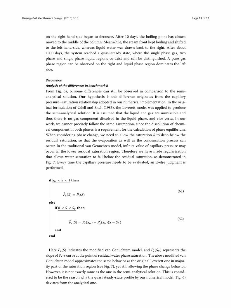
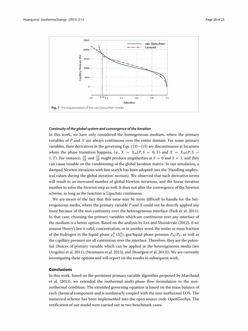
From Fig. 6a, b, some differences can still be observed in comparison to the semi-analytical solution. Our hypothesis is this difference originates from the capillarypressure−saturation relationship adopted in our numerical implementation. In the orig-inal formulation of Udell and Fitch (1985), the Leverett model was applied to producethe semi-analytical solution. It is assumed that the liquid and gas are immiscible andthus there is no gas component dissolved in the liquid phase, and vice versa. In ourwork, we cannot precisely follow the same assumption, since the dissolution of chemi-cal component in both phases is a requirement for the calculation of phase equilibrium.When considering phase change, we need to allow the saturation S to drop below theresidual saturation, so that the evaporation as well as the condensation process canoccur. In the traditional van Genuchten model, infinite value of capillary pressure mayoccur in the lower residual saturation region. Therefore we have made regularizationthat allows water saturation to fall below the residual saturation, as demonstrated inFig. 7. Every time the capillary pressure needs to be evaluated, an if-else judgment isperformed.

if Slr < S < 1 then

P̄c(S) = Pc(S)(61)

elseif 0 < S < Slr then

P̄c(S) = Pc(Slr) − P′c(Slr)(S − Slr)

(62)

endend

Here P̄c(S) indicates the modified van Genuchtem model, and P′c(Slr) represents the

slope of Pc-S curve at the point of residual water phase saturation. The abovemodified vanGenuchten model approximates the same behavior as the original Leverett one in major-ity part of the saturation region (see Fig. 7), yet still allowing the phase change behavior.However, it is not exactly same as the one in the semi-analytical solution. This is consid-ered to be the reason why the quasi steady-state profile by our numerical model (Fig. 6)deviates from the analytical one.

Huang et al. Geothermal Energy (2015) 3:13 Page 20 of 23

Fig. 7 The regularization of the van Genuchten model

Continuity of the global system and convergence of the iteration

In this work, we have only considered the homogeneous medium, where the primaryvariables of P and X are always continuous over the entire domain. For some primaryvariables, their derivatives in the governing Eqs. (13)−(15) are discontinuous at locationswhere the phase transition happens, i.e., X = Xm(P, S = 0,T) and X = XM(P, S =1,T). For instance, ∂S

∂X and ∂S∂P might produce singularities at S = 0 and S = 1, and they

can cause trouble on the conditioning of the global Jacobian matrix. In our simulation, adamped Newton iterations with line search has been adopted (see the ‘Handling unphys-ical values during the global iteration’ section). We observed that such derivative termswill result in an increased number of global Newton iterations, and the linear iterationnumber to solve the Newton step as well. It does not alter the convergence of the Newtonscheme, as long as the function is Lipschitz continuous.We are aware of the fact that this issue may be more difficult to handle for the het-

erogeneous media, where the primary variable P and X could not be directly applied anymore because of the non-continuity over the heterogeneous interface (Park et al. 2011).In that case, choosing the primary variables which are continuous over any interface ofthe medium is a better option. Based on the analysis by Ern and Mozolevski (2012), if weassume Henry’s law is valid, concentration, or in another word, the molar or mass fractionof the hydrogen in the liquid phase ρh

L (XhL), gas/liquid phase pressure PG/PL, as well as

the capillary pressure are all continuous over the interface. Therefore, they are the poten-tial choices of primary variable which can be applied in the heterogeneous media (see(Angelini et al. 2011); (Neumann et al. 2013), and (Bourgeat et al. 2013)). We are currentlyinvestigating these options and will report on the results in subsequent work.

ConclusionsIn this work, based on the persistent primary variable algorithm proposed by Marchandet al. (2013), we extended the isothermal multi-phase flow formulation to the non-isothermal condition. The extended governing equation is based on the mass balance ofeach chemical component and is nonlinearly coupled with the non-isothermal EOS. Thenumerical scheme has been implemented into the open source code OpenGeoSys. Theverification of our model were carried out in two benchmark cases.

Huang et al. Geothermal Energy (2015) 3:13 Page 21 of 23

• For the GNR MoMaS (Bourgeat et al. 2009) benchmark (‘Benchmark I: isothermalinjection of H2 gas’ section), the extended model is capable of simulating themigration of H2 gas including its dissolution in aqueous phase. The simulated resultsfitted well with those from other codes (Marchand et al. 2013; Marchand andKnabner 2014).

• For the non-isothermal benchmark, we simulated the heat pipe problem and verifiedour result against the semi-analytical solution (‘Benchmark II: heat pipe problem’section). Furthermore, our numerical model extended the original heat pipe problemto include the phase change behavior.

Currently, we are working on the incorporation of equilibrium reactions, such as themineral dissolution and precipitation, into the EOS system. As our global mass-balanceequations are already component based, one governing equation can be written for eachbasis component. Pressure, temperature, and molar fraction of the chemical componentscan be chosen as primary variables. Inside the EOS problem, the amount of secondarychemical components can be calculated based on the result of basis, which can furtherlead to the phase properties as density and viscosity. The full extension of includingtemperature-dependent reactive transport system will be the topic of a separate work inthe near future.

NomenclatureGreek symbolsε Tolerance value for Newton iteration. [-]λT Heat Conductivity. [W m−1 K−1]μα Viscosity in α phase. [Pa · s]νiα Chemical potential of i-component in α phase. [Pa]� Porosity. [-]φi

α fugacity coefficient of i-component in α phase. [-]ρi

α Mass density of i-component in α phase. [Kg m−3]

Operators

∧ Logical "and"‖‖2 Euclidean normΨ (a, b) Minimum function

Roman symbols

g Vector for gravitational force. [m s−2]cpα Specific heat capacity in phase α at given pressure. [J Kg−1 K−1]cS Specific heat capacity of soil grain. [J Kg−1 K−1]Di

α Diffusion coefficient of i-component in phase α. [m2 s−1]Fi Mass source/sink term for i-component. [Kg m−3 s−1]f iα Fugacity of i-component in α phase. [Pa]HhW Henry coefficient. [mol Pa−1 m−3]

hα Specific enthalpy. [J Kg−1]jiα Diffusive mass flux of i-component in α phase. [mol m−2 s−1]K Intrinsic Permeability. [m2]Nα Molar density in α phase. [mol m−3]Pα Pressure in α phase. [Pa]PwGvapor Vapor pressure of pure water. [Pa]Pc Capillary pressure. [Pa]QT Heat source/sink term. [W s−2]

Huang et al. Geothermal Energy (2015) 3:13 Page 22 of 23

R Universal Gas Constant. [J mol−1 K−1]Sαr Residual saturation in α phase. [-]Sα Saturation in α phase. [-]Sle Effective saturation. [-]T Temperature. [K]uα Specific internal energy. [J Kg−1]Vα Volume in α phase. [m3]vα Darcy velocity in α phase. [m s−1]X Total molar fraction of light component in two phases. [-]Xi

α Molar Fraction of i-component in α phase. [-]

Additional files

Additional file 1: This document introduces how this analytical solution is deducted.

Additional file 2: This is the main matlab script file, which will be executed to produce the analytical solution.

Additional file 3: This file constructs the four coupled differential equations.

Additional file 4: This file calculates the relative permeability of gas phase.

Additional file 5: This file calculates the relative permeability of liquid phase.

Additional file 6: This file calculates the capillary pressure, with water saturation as the input parameter.

Competing interestsThe authors declare that they have no competing interests.

Authors’ contributionsYH implemented the extended method into the OpenGeoSys software, produced simulation results of the twobenchmarks, and also drafted this manuscript. HS designed the numerical algorithm of solving the coupled PDEs, andalso contributed to the code implementation. OK coordinated the development of OpenGeoSys, and contributed to themanuscript writing. All authors read and approved the final manuscript.

AcknowledgementsWe would thank to Dr. Norihito Watanabe for his thoughtful scientific suggestions and comments on this paper. Thiswork has been funded by the Helmholtz Association through the program POF III-R41 ‘Geothermal Energy Systems’. Thefirst author would also like to acknowledge the financial support from Chinese Scholarship Council (CSC).

Author details1Helmholtz Centre for Environmental Research - UFZ, Permoserstr. 15, 04318 Leipzig, Germany. 2Technical University ofDresden, Helmholtz-Strane 10, 01062 Dresden, Germany. 3Freiberg University of Mining and Technology,Gustav-Zeuner-Strasse 1, 09596 Freiberg, Germany.

Received: 17 December 2014 Accepted: 7 May 2015

ReferencesAbadpour A, Panfilov M (2009) Method of negative saturations for modeling two-phase compositional flow with

oversaturated zones. Transp Porous Media 79(2):197–214Angelini O, Chavant C, Chénier E, Eymard R, Granet S (2011) Finite volume approximation of a diffusion–dissolution

model and application to nuclear waste storage. Math Comput Simul 81(10):2001–2017Ben Gharbia I, Jaffré J (2014) Gas phase appearance and disappearance as a problem with complementarity constraints.

Math Comput Simul 99:28–36Bourgeat A, Jurak M, Smaï F (2009) Two-phase, partially miscible flow and transport modeling in porous media;

application to gas migration in a nuclear waste repository. Comput Geosci 13(1):29–42Bourgeat, A, Jurak M, Smaï F (2013) On persistent primary variables for numerical modeling of gas migration in a nuclear

waste repository. Comput Geosci 17(2):287–305Çengel YA, Boles MA (1994) Thermodynamics: an engineering approach. Property Tables, Figures and Charts to

Accompany. McGraw-Hill Ryerson, Limited, Singapore. https://books.google.de/books?id=u2-SAAAACAAJClass H, Helmig R, Bastian P (2002) Numerical simulation of non-isothermal multiphase multicomponent processes in

porous media: 1. an efficient solution technique. Adv Water Resour 25(5):533–550Ern A, Mozolevski I (2012) Discontinuous galerkin method for two-component liquid–gas porous media flows. Comput

Geosci 16(3):677–690Fatt I, Klikoff Jr WA (1959) Effect of fractional wettability on multiphase flow through porous media. Trans., AIME (Am. Inst.

Min. Metall. Eng.), 216:426–432Forsyth P, Shao B (1991) Numerical simulation of gas venting for NAPL site remediation. Adv Water Resour 14(6):354–367Gawin D, Baggio P, Schrefler BA (1995) Coupled heat, water and gas flow in deformable porous media. Int J Numer

Methods Fluids 20(8-9):969–987. doi:10.1002/fld.1650200817Hassanizadeh M, Gray WG (1980) General conservation equations for multi-phase systems: 3. constitutive theory for

porous media flow. Adv Water Resour 3(1):25–40

Huang et al. Geothermal Energy (2015) 3:13 Page 23 of 23

Helmig R (1997) Multiphase flow and transport processes in the subsurface: a contribution to the modeling ofhydrosystems. Springer, Berlin

Kanzow C (2004) Inexact semismooth newton methods for large-scale complementarity problems. OptimizationMethods Softw 19(3-4):309–325

Kolditz O, De Jonge J (2004) Non-isothermal two-phase flow in low-permeable porous media. Comput Mech33(5):345–364

Kolditz O, Bauer S, Bilke L, Böttcher N, Delfs JO, Fischer T, Görke UJ, Kalbacher T, Kosakowski G, McDermott CI,Park CH, Radu F, Rink K, Shao H, Shao HB, Sun F, Sun YY, Singh AK, Taron J, Walther M, Wang W, Watanabe N,Wu Y, Xie M, Xu W, Zehner B (2012) Opengeosys: an open-source initiative for numerical simulation ofthermo-hydro-mechanical/chemical (THM/C) processes in porous media. Environ Earth Sci 67(2):589–599.http://dx.doi.org/10.1007/s12665-012-1546-x

Kräutle S (2011) The semismooth newton method for multicomponent reactive transport with minerals. Adv WaterResour 34(1):137–151

Landau L, Lifshitz E (1980) Statistical physics, part i. Course Theoretical Phys 5:468Marchand E, Müller T, Knabner P (2012) Fully coupled generalised hybrid-mixed finite element approximation of

two-phase two-component flow in porous media. part ii: numerical scheme and numerical results. Comput Geosci16(3):691–708

Marchand, E, Müller T, Knabner P (2013) Fully coupled generalized hybrid-mixed finite element approximation oftwo-phase two-component flow in porous media. part i: formulation and properties of the mathematical model.Comput Geosci 17(2):431–442

Marchand E, Knabner P (2014) Results of the momas benchmark for gas phase appearance and disappearance usinggeneralized mhfe. Adv Water Resour 73:74–96

Neumann R, Bastian P, Ippisch O (2013) Modeling and simulation of two-phase two-component flow with disappearingnonwetting phase. Comput Geosci 17(1):139–149

Olivella S, Gens A (2000) Vapour transport in low permeability unsaturated soils with capillary effects. Transp PorousMedia 40(2):219–241

Park CH, Taron J, Görke UJ, Singh AK, Kolditz O (2011) The fluidal interface is where the action is in CO2 sequestration andstorage: Hydro-mechanical analysis of mechanical failure. Energy Procedia 4:3691–3698

Panfilov M, Panfilova I (2014) Method of negative saturations for flow with variable number of phases in porous media:extension to three-phase multi-component case. Comput Geosci:1–15

Park CH, Böttcher N, Wang W, Kolditz O (2011) Are upwind techniques in multi-phase flow models necessary?. J ComputPhys 230(22):8304–8312

Pruess K (2008) On production behavior of enhanced geothermal systems with CO2 as working fluid. Energy ConversManag 49(6):1446–1454

Peng DY, Robinson DB (1976) A new two-constant equation of state. Ind Eng Chem Fundam 15(1):59–64Salimi H, Wolf KH, Bruining J (2012) Negative saturation approach for non-isothermal compositional two-phase flow

simulations. Transp Porous Media 91(2):391–422Singh A, Baumann G, Henninges J, Görke UJ, Kolditz O (2012) Numerical analysis of thermal effects during carbon dioxide

injection with enhanced gas recovery: a theoretical case study for the altmark gas field. Environ Earth Sci 67(2):497–509Singh A, Delfs JO, Böttcher N, Taron J, Wang W, Görke UJ, Kolditz O (2013a) A benchmark study on non-isothermal

compositional fluid flow. Energy Procedia 37:3901–3910Singh A, Delfs JO, Shao H, Kolditz O (2013b) Characterization of co2 leakage into the freshwater body. In: EGU General

Assembly Conference Abstracts Vol. 15. p 11474Udell K, Fitch J (1985) Heat and mass transfer in capillary porous media considering evaporation, condensation, and

non-condensible gas effects. In: 23rd ASME/AIChE National Heat Transfer Conference, Denver, CO. pp 103–110Van Genuchten MT (1980) A closed-form equation for predicting the hydraulic conductivity of unsaturated soils. Soil Sci

Soc Am J 44(5):892–898Wu YS, Forsyth PA (2001) On the selection of primary variables in numerical formulation for modeling multiphase flow in

porous media. J Contam Hydrol 48(3):277–304

Submit your manuscript to a journal and benefi t from:

7 Convenient online submission

7 Rigorous peer review

7 Immediate publication on acceptance

7 Open access: articles freely available online

7 High visibility within the fi eld

7 Retaining the copyright to your article

Submit your next manuscript at 7 springeropen.com