USING REGIONAL CLIMATE MODELS TO

SIMULATE HYDROMETEOROLOGICAL

PROCESSES OVER EUROPE

D i ss e r ta t i on z u r Er l angung des Dok to rg rades an de r Faku l t ä t f ü r

Geow iss ens cha f ten de r Ludw ig -M ax im i l i ans - Un iv e rs i t ä t Münc hen

v o rge leg t von

Ben jam in Posch lod

a us M ünc hen

e i ngere i ch t am 07 .0 9 .2020 , München

Date of the application for admission to the doctoral procedure: 20.12.2018

Date of the disputation: 17.12.2020

Supervisor: Prof. Dr. Ralf Ludwig, Department of Geography, Ludwig-Maximilians-Universität,

Munich, Germany

2nd supervisor: Dr. Jana Sillmann, Center for International Climate Research, Oslo, Norway

Date of the oral examination: XX.XX.2020

Acknowledgments

This thesis represents an important step in my scientific and professional career, which I owe

in this form to a number of people to whom I would like to express my deepest gratitude in the

following.

First, I want to thank Prof. Dr. Ralf Ludwig for giving me the opportunity to start my doctorate

and conduct my research under his supervision. I am grateful for his professional advice, our

trustful relationship and for giving me the possibility to spend some time for further educational

trips in Germany and abroad. Furthermore, my entire education as natural scientist, from bach-

elor to doctorate, benefited greatly from his dedication to teaching, his supervision of the Bach-

elor’s and Master‘s courses, and his support during the doctorate.

Special thanks goes to Dr. Jana Sillmann, who welcomed me at CICERO and supervised me

during a research internship in Oslo and accompanied me during my doctorate in the context

of my research and publications. Moreover, I want to thank her whole research group as well

as Gunnar, Kari and Øivind at CICERO, who welcomed me very friendly and took their time to

discuss and support my work at an early stage of my career.

Another cordial thanks goes to Dr. Jakob Zscheischler, who introduced me to the world of

compound events and multivariate statistics. I am also very grateful to him and all other organ-

izers for the invitation to the “Training School on Statistical Modelling of Compound Events“ in

Como. It was an instructive and exciting time during which I was able to meet future colleagues

and make friendships.

I am also grateful to Julia Schneider and Flo Zabel for our regular visits to Baresta, which

combined Italian coffee pleasure and discussions about science, non-science and basically

anything under the sun. Further, I want to thank my officemates and project colleagues Andrea

and Magdalena for fruitful discussions and the collaboration within many short-duration pro-

jects. Also, I am grateful to the whole “ClimEx-group“ Flo, Raul and Fabi for their big amount

of work within the ClimEx project, for their advices, and help with Matlab or Python. Also a

warm thanks to Vera Erfurth for handling all the bureaucratic work for me, ranging from con-

tracts, permits to approvals and while always being available for a nice talk.

Finally, I want to thank my partner Susi, who accompanied and supported me throughout my

time at the university and diverted me from my work at the right moments. I also thank my

family, and all my friends (especially the best Master’s class of all times) for their support and

confidence in me.

Zusammenfassung I

Zusammenfassung

Klima ist ein dynamisches und komplexes System, das durch seine Strahlungs- und Energie-

bilanz, atmosphärische Zirkulationssysteme, Interaktionen zwischen Boden und Atmosphäre

sowie durch die geographische Breite, Topographie und viele weitere Zusammenhänge be-

stimmt wird. Globale Klimamodelle simulieren die damit verbundenen Prozesse auf Basis phy-

sikalischer Zusammenhänge, wobei sie in ihrer Eigenschaft als Modell die Abläufe vereinfa-

chend abbilden und die Ergebnisse verschiedenen Unsicherheiten unterliegen. Um die Reprä-

sentation dieser natürlichen Prozesse auf regionaler Ebene zu verbessern, werden regionale

Klimamodelle (RCM) eingesetzt, die die Simulationen globaler Modelle dynamisch in eine hö-

here Auflösung skalieren. Gerade für heterogene Regionen wie Europa, das über eine kom-

plexe Topographie verfügt sowie von starken Nord-Süd und West-Ost Gradienten bei Lufttem-

peratur und Feuchte gekennzeichnet ist, erhöhen regionale Klimamodelle die Qualität der Er-

gebnisse.

Die Hydrometeorologie beschäftigt sich dabei mit allen Komponenten des Wasserkreislaufs,

nämlich Verdunstung, Niederschlag, Abfluss und Speicherung. Damit bewegt sich die Hydro-

meteorologie in einem Überlappungsbereich der Meteorologie, Klimatologie und Hydrologie.

Die vorliegende Doktorarbeit behandelt anhand vier wissenschaftlicher Veröffentlichungen

ausgewählte hydrometeorologische Prozesse auf lokaler bis kontinentaler Ebene, deren Si-

mulation mithilfe regionaler Klimamodelle mittels observierter Daten evaluiert wird. Es handelt

sich dabei um (1) Extremniederschlag in Europa, (2) zusammengesetzte Ereignisse (com-

pound events) aus Starkniederschlag und Schneeschmelze sowie Starkniederschlag und ho-

her Bodenfeuchte in der südlichen Hälfte Norwegens, (3) die Saisonalität und Abflusshöhe der

Flussregime in Bayern, und (4) die lokalen Niederschlagseigenschaften in Oslo, Norwegen.

Neben der Validierung der Modellergebnisse durch Messdaten liegt ein besonderes Augen-

merk auf der Diskussion von Unsicherheiten. Klimaprojektionen unterliegen dabei zwei großen

Quellen für Unsicherheit. Die Vereinfachungen der physikalischen Prozesse in Klimamodellen

führt zur Modellunsicherheit, weshalb unterschiedliche Klimamodelle unter denselben Rand-

bedingungen abweichende Ergebnisse erzeugen. Der zweite Unsicherheitsfaktor liegt in der

internen Variabilität des Klimasystems begründet. Ein einziges Klimamodell berechnet be-

trächtlich voneinander abweichende Simulationen, wenn sich die Startbedingungen des Mo-

dells auch nur minimal unterscheiden. Diese Schwankungsbreite der Ergebnisse kann als

Bandbreite interpretiert werden, innerhalb derer das reale Klima variieren kann.

Eine dritte Unsicherheitsquelle ergibt sich dann, wenn Projektionen zukünftige klimatische Ver-

hältnisse abbilden sollen. Das zugrundeliegende Emissionsszenario ist unsicher, da die zu-

künftigen Emissionen nicht bekannt sind, aber im Rahmen von Szenarien geschätzt werden.

II

Die ersten drei Publikationen behandeln ihren thematischen Schwerpunkt anhand eines Mo-

dellensembles des kanadischen regionalen Klimamodells Version 5 (CRCM5) mit einer räum-

lichen Auflösung von 12 km. Dieses RCM wurde 50-mal mit gering abweichenden Startbedin-

gungen gerechnet, um die interne Variabilität des Klimasystems in Europa zu repräsentieren,

was als „single model initial-condition large ensemble“ (SMILE) bezeichnet wird. Die Klimapro-

jektionen reichen in die Zukunft bis zum Jahr 2099, wobei den Modellrechnungen das extreme

Emissionsszenario RCP 8.5 ab 2006 zugrunde liegt. Die Ergebnisse der ersten drei Studien

sollen im Folgenden zusammenfassend präsentiert werden: (1) Das CRCM5 Ensemble ist ge-

eignet, um Extremniederschlagshöhen für Dauerstufen zwischen 3 und 24 Stunden zu simu-

lieren. Die observationsbasierten Daten aus 16 Ländern und 32 Quellen stehen in etwa 80 %

der Landfläche in Übereinstimmung mit den Modellergebnissen, wobei sich die größten Dis-

krepanzen in topographisch komplexen Regionen und Gebieten mit häufiger und starker Kon-

vektion ergeben. Die Schwankungsbreite der internen Variabilität ergibt eine Unsicherheit von

etwa -15 % bis +18 %. Der sich daraus ergebende Datensatz mit Niederschlagshöhen der

Jährlichkeit 10 a wurde für jedermann zugänglich veröffentlicht. (2) Das CRCM5 Ensemble

kann das Timing von Starkniederschlagsereignissen, die gleichzeitig mit Schneeschmelze o-

der hoher vorhergehender Bodenfeuchte auftreten, für die Region Südnorwegen reproduzie-

ren. In einem quantil-basierten Framework wurden die Zeitrahmen 1980–2009 und 2070–2099

verglichen. Durch den Klimawandel verringert sich die Eintrittswahrscheinlichkeit von Stark-

niederschlag und Schneeschmelze um 48 %, wohingegen sich die Wahrscheinlichkeit von

Starkniederschlag auf gesättigten Boden um 38 % erhöht. Die interne Variabilität des Kli-

masystems bedingt dabei eine große Varianz in den Eintrittswahrscheinlichkeiten dieser biva-

riaten Ereignisse. (3) An das CRCM5 Ensemble wurde das hydrologische Modell WaSiM ge-

koppelt, um den Abfluss in 98 Flusseinzugsgebieten in und um Bayern zu simulieren. Die Sai-

sonalität der Abflüsse kann mit einem Fehler von 9% reproduziert werden. Die Gruppierung

der 98 Einzugsgebiete mittels eines agglomerativen hierarchischen Clusteringverfahrens

ergibt sechs Klassen an Abflussregimen. Durch das sich im Verhältnis zum Zeitraum 1981–

2010 ändernde Klima verschiebt sich die räumliche Ausbreitung dieser Klassen, so dass bis

2011–2040 etwa 8 %, bis 2041–2070 etwa 23 %, und bis 2071–2099 etwa 43 % der Einzugs-

gebiete einer anderen Regimeklasse zugehörig sein werden. Die Verwendung eines Ensem-

bles mit 50 Klimarealisationen trägt dabei maßgeblich zur Robustheit des Clusteringverfahrens

bei und verringert Unsicherheiten durch die interne Variabilität.

Die vierte Veröffentlichung basiert auf einem Datensatz, der mithilfe des sehr hoch aufgelösten

Weather and Research Forecasting Model (WRF; 3 km räumliche Auflösung) über einer Do-

mäne in Südnorwegen erzeugt wurde. Während RCMs mit einer gröberen Auflösung als 4 km

konvektive Prozesse mittels statistischer Parametrisierungen umschreiben müssen, wird Kon-

Zusammenfassung III

vektion in höher aufgelösten Modellen explizit simuliert. Die Studie hat dabei untersucht, in-

wieweit die Niederschlagscharakteristika von zehn Messstationen im Großraum Oslo zwi-

schen 2000 und 2017 durch das RCM reproduziert werden können. Das RCM wurde dabei

von Reanalysedaten angetrieben, um Kontinuität mit den Beobachtungen zu gewährleisten.

Es konnten das Verhältnis von trockenen zu nassen Stunden, die zeitliche Autokorrelation, die

Anzahl feuchter Stunden im Monat, die Anzahl und Dauer nasser Perioden, die räumliche Kor-

relation, und die Intensitäten von Starkniederschlägen für Aggregationen von 6 und 12 Stun-

den mit Abweichungen von weniger als 10 % reproduziert werden. Starkniederschläge zwi-

schen 1 und 3 Stunden wurden unterschätzt.

Auch wenn alle vier Publikationen unterschiedliche Teilbereiche der Hydrometeorologie in ver-

schiedenen Regionen untersucht haben, ergeben sich aus diesen Studien dennoch wertvolle

und allgemeingültige Erkenntnisse für die Forschungsgemeinschaft im Bereich der regionalen

Klimamodellierung, die sich wie folgt zusammenfassen lassen. Interne Variabilität spielt eine

große Rolle bei der Abschätzung von Extremniederschlägen, bei der Auftrittswahrscheinlich-

keit von zusammengesetzten Ereignissen, aber auch bei der Saisonalität aller Komponenten

des Wasserkreislaufs. Die damit verbundene Unsicherheit lässt sich mithilfe von SMILEs

quantifizieren. Diese Unsicherheiten treten nicht nur bei der Nutzung einzelner Modellläufe

von Klimamodellen auf, sondern auch bei der Applikation von Observationsdaten. Das ver-

gangene Klima ist seinerseits nur eine der unendlich vielen möglichen Realisationen des Kli-

mas im Rahmen seiner internen Variabilität. Dementsprechend bilden SMILEs eine wertvolle

Datenbasis, um sehr seltene oder extreme Ereignisse zu detektieren und ihre Wahrscheinlich-

keiten einzuschätzen. Während die momentan räumlich am höchsten aufgelösten Ensembles

Gitterzellen mit 12 x 12 km² aufweisen, hat die vierte Publikation gezeigt, dass höhere Auflö-

sungen es ermöglichen, komplexe Topographie abzubilden und zeitliche wie räumliche Nie-

derschlagscharakteristika auf lokaler Ebene zu simulieren.

Es wäre daher für zukünftige Projekte von großem Nutzen, SMILEs in einer räumlichen Auflö-

sung zu erschaffen, die konvektive Prozesse und komplexe Topographie abbilden können.

Diese Modellrechnungen wären allerdings aufgrund der immensen Anforderungen an die

Hochleistungsrechenzentren nur unter einer weiterhin exponentiellen Entwicklung der Re-

chenleistung in absehbarer Zukunft realistisch.

IV

Summary

Climate is a dynamic and complex system that is determined by its radiation and energy bal-

ance, atmospheric circulation systems, soil-atmosphere interactions, latitude, topography and

many other interrelationships. Global climate models simulate the associated processes on

the basis of physical equations and relationships. In their capacity as models, they simplify the

processes and the results are subject to various uncertainties. In order to improve the repre-

sentation of these natural processes on a regional level, regional climate models (RCM) are

used, which dynamically downscale the simulations of global models to a higher resolution.

Especially for heterogeneous regions such as Europe, which has a complex topography and

is characterized by strong north-south and west-east gradients in air temperature and humidity,

regional climate models increase the quality of the results.

Hydrometeorology addresses all components of the hydrological cycle, namely evaporation,

precipitation, runoff and storage. Hydrometeorology is thus in an overlapping area of meteor-

ology, climatology and hydrology.

The present doctoral thesis deals with selected hydrometeorological processes on a local to

continental level, where the simulation of these processes by regional climate models is eval-

uated using observed data. These processes are (1) extreme precipitation in Europe, (2) com-

pound events consisting of joint heavy precipitation and snowmelt as well as joint heavy pre-

cipitation and high soil moisture in the southern half of Norway, (3) the seasonality and runoff

levels of river regimes in Bavaria, and (4) local precipitation characteristics in Oslo, Norway.

Besides the validation of the model results by measured data, special attention is paid to the

discussion of uncertainties. Climate projections are subject to two major sources of uncertainty.

The simplification of physical processes in climate models leads to model uncertainty, which

is why different climate models produce different results despite being driven by the same

boundary conditions. The second source of uncertainty is the internal variability of the climate

system. A single climate model produces simulations that differ considerably from each other

even if the initial conditions of the model differ minimally. This variability of the results can be

interpreted as the range within which the real climate can vary.

A third source of uncertainty arises when projections try to reflect future climatic conditions.

The underlying emission scenario is uncertain because the future emissions are not known,

but are estimated within the framework of emission scenarios.

Within the first three publications the research is conducted applying an ensemble of the Ca-

nadian Regional Climate Model version 5 (CRCM5) with a spatial resolution of 12 km. This

RCM was run 50 times with slightly different initial conditions to represent the internal variability

of the climate system in Europe, which is called a single model initial-condition large ensemble

Summary V

(SMILE). The climate projections extend into the future up to the year 2099, with the model

calculations being based on the extreme emission scenario Representative Concentration

Pathways (RCP) 8.5 from 2006 onwards. The results of the first three studies will be presented

in the following: (1) The CRCM5 ensemble is suitable for simulating extreme precipitation lev-

els for durations between 3 and 24 hours. The observation-based data from 16 countries and

32 sources are consistent with the model results in about 80 % of the land area, with the largest

deviations in topographically complex regions and areas with frequent and strong convection.

The range of internal variability results in an uncertainty of about -15 % to +18 %. The resulting

dataset with 10-year return levels has been published for public access. (2) The CRCM5 en-

semble can reproduce the timing of heavy precipitation events occurring simultaneously with

snow melt or high preceding soil moisture for the region of Southern Norway. In a quantile-

based framework the time frames 1980–2009 and 2070–2099 were compared. Climate

change reduces the probability of occurrence of heavy precipitation and snowmelt by 48 %,

whereas the probability of heavy precipitation on saturated soil increases by 38 %. The internal

variability of the climate system causes a large variance in the occurrence probabilities of these

bivariate events. (3) The hydrological model WaSiM was coupled to the CRCM5 ensemble to

simulate runoff in 98 river basins in and around Bavaria. The seasonality of the discharges can

be reproduced with an error of 9 %. The grouping of the 98 river basins by means of an ag-

glomerative hierarchical clustering method results in six classes of runoff regimes. Due to the

changing climate in relation to the period 1981–2010 the spatial distribution of these classes

shifts, so that by 2011–2040 about 8 %, by 2041–2070 about 23 %, and by 2071–2099 about

43 % of the catchments will belong to another regime class. The use of an ensemble with 50

climate realizations contributes significantly to the robustness of the clustering results and re-

duces uncertainties due to internal variability.

The fourth publication is based on a data set generated using the very high resolution Weather

and Research Forecasting Model (WRF; 3 km spatial resolution) over a domain in southern

Norway. While RCMs with a resolution broader than 4 km have to describe convective pro-

cesses by statistical parameterizations, convection is explicitly simulated in higher resolution

models. The study investigated to what extent the precipitation characteristics of ten rain

gauges in the Oslo area can be reproduced by the RCM between 2000 and 2017. The RCM

was driven by reanalysis data to ensure continuity with the observations. The dry proportion,

the temporal autocorrelation, the number of wet hours per month, the number and duration of

wet spells, the spatial correlation, and the intensities of 6- and 12-hourly heavy precipitation

could be reproduced with deviations of less than 10 %. Hourly and 3-hourly heavy precipitation

was underestimated.

Even though all four publications have investigated different sub-areas of hydrometeorology in

various regions, these studies nevertheless provide valuable and generally valid findings for

VI

the research community in the field of regional climate modelling, which can be summarised

as follows. Internal variability plays a major role in the estimation of extreme precipitation, in

the probability of occurrence of compound events, but also in the seasonality of all components

of the hydrological cycle. The associated uncertainty can be quantified using SMILEs. These

uncertainties occur not only when using individual model runs of climate models, but also when

applying observation data. The past climate is only one of the possible realizations of the cli-

mate within the range of its internal variability. Accordingly, SMILEs provide a valuable data-

base for detecting very rare or extreme events and estimating their probabilities. While the

currently highest spatially resolved SMILEs have grid cells with 12 x 12 km², the fourth publi-

cation has shown that higher resolutions allow to map complex topography and to simulate

temporal and spatial precipitation characteristics on a local scale.

Therefore, it would be of great benefit for future projects to create SMILEs in a spatial resolution

that is able to resolve convective processes and complex topography. However, due to the

immense demands on high-performance computing centres, these model runs would only be

realistic in the foreseeable future if computing power continued to develop exponentially.

Table of Contents VII

Table of Contents

Page

Zusammenfassung I

Summary IV

Table of Contents VII

Abbreviations IX

List of Figures X

1 Introduction 11

1.1 Climate models 11

1.1.1 History of numerical climate models 11

1.1.2 How climate models work 12

1.1.3 Why should we use regional climate models? History, problems, added value

and the current state 14

1.1.4 Using regional climate models to drive impact models 20

1.2 Uncertainties 21

1.2.1 Uncertainties of climate model projections 21

1.2.2 Observational uncertainty 23

1.2.3 Uncertainty due to bias adjustment 24

1.2.4 Uncertainty of hydrological impact models 26

1.3 Thematic focus and associated research questions 26

2 Publications 29

2.1 Publication I: Return levels of sub-daily extreme precipitation over Europe (Earth

System Science Data) 31

2.2 Transition to Publication II 67

2.3 Publication II: Climate change effects on hydrometeorological compound events

over southern Norway (Weather and Climate Extremes) 68

2.4 Transition to Publication III 81

2.5 Publication III: Impact of Climate Change on the Hydrological Regimes in Bavaria

(Water) 82

VIII

2.6 Transition to Publication IV 104

2.7 Publication IV: Comparison and Evaluation of Statistical Rainfall Disaggregation

and High-Resolution Dynamical Downscaling over Complex Terrain (Journal of

Hydrometeorology) 105

3 Conclusion and Outlook 117

References 123

Abbreviations IX

Abbreviations

AOGCM Atmosphere-Ocean General Circulation Model

AORCM Atmosphere-Ocean Regional Climate Model

BA Bias Adjustment

CanESM2 Canadian Earth System Model version 2

CPM Convection-Permitting Model

CRCM5 Canadian Regional Climate Model version 5

ESM Earth System Model

GCM General Circulation Model / Global Climate Model

IPCC Intergovernmental Panel on Climate Change

LAM Limited-Area Model

LBC Lateral Boundary Conditions

LSM Land Surface Model

MME Multi-Model Ensemble

MoF Method of Fragments

NWP Numerical Weather Prediction

RCM Regional Climate Model

RCP Representative Concentration Pathways

RESM Regional Earth System Model

SMILE Single Model Initial-condition Large Ensemble

WaSiM Water balance Simulation Model

WRF Weather Research and Forecasting Model

X

List of Figures

Page

Figure 1: Schematic representation of a one-dimensional radiative-convective model. 12

Figure 2: Schematic representation of an atmosphere-ocean general circulation model

(AOGCM; adapted from NOAA 2020). 14

Figure 3: Representation of the topography in the western United States by (a) 500 km

resolution and (b) 50 km resolution (adapted from Giorgi, 2019). 15

Figure 4: Schematic representation of dynamical downscaling via one-way nesting. 17

Figure 5: Relative contribution of internal variability, scenario uncertainty and model

uncertainty to overall uncertainty of the climate projection (adapted from Hawkins & Sutton,

2009). 22

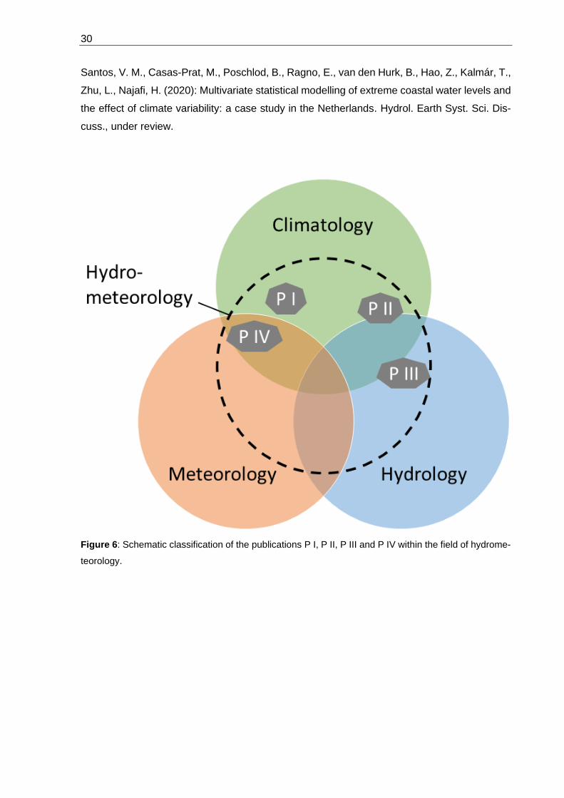
Figure 6: Schematic classification of the publications P I, P II, P III and P IV within the field of

hydrometeorology. 30

Introduction 11

1 Introduction

First, a short introduction to the topic of climate modelling shall be given in order to provide an

overview of the history, the current state of research and the uncertainties associated with

climate modelling. Further, the thematic focus of this dissertation will be described in an intro-

ductory way and the research questions that will be addressed in the four publications will be

defined.

1.1 Climate models

1.1.1 History of numerical climate models

Climate models as such try to represent the real climate system, but in their capacity as models

they can only embody an approximation of reality. The main tasks of climate models, however,

consist in two major fields (Flato et al., 2013): (1) Improvement of the understanding of the

climate system including its feedbacks and complex interactions, and (2) creating projections

of future climate conditions covering time periods of the century scale. There are different ways

to capture climatic processes in a simplified form, such as a purely descriptive approach, a

statistical approach or an approach based on physical relationships. Here, only climate models

applying quantitative methods are introduced, which are often referred to as numerical climate

models (McGuffie & Henderson-Sallers, 2001). As the climate system is governed by mass

and energy fluxes on several scales, the simplest model describes the radiation equilibrium of

the Earth,

(1 − 𝛼)𝑆𝜋𝑟2 = 4𝜋𝑟2𝜖𝜎𝑇4 (1),

where the left part of the equation defines the incoming shortwave radiation and the right part

represents the outgoing longwave radiation following the Stefan-Boltzmann law. Thereby, α is

the albedo of the Earth (~ 0.3), S the solar constant (1367 W/m²), and r the radius of the Earth

(6371 ×106 m). ϵ represents the effective emissivity of the Earth (~ 0.612) and σ is the Stefan-

Boltzmann constant amounting to approximately 5.67×10−8 J·K−4·m−2·s−1. Equation 1 can be

solved to achieve the average radiative temperature of the Earth T:

𝑇 = √(1−𝛼)𝑆

4𝜖𝜎

4 (2),

where T amounts to ~ 288.15 K or 15.15 °C. This model inhibits a large degree of simplification,

as neither the spatial distribution nor any mass and energy fluxes on Earth are represented.

Therefore, it is called zero-dimension model (McGuffie & Henderson-Sallers, 2001). Within the

model, the albedo α and the emissivity ϵ represent dynamic terms, which are affected by land

cover and climate change.

12

Adding a vertical component leads to a one-dimensional model, which is referred to as radia-

tive-convective model. There, the thermal (vertical) structure of the atmosphere is included by

representing up- and downwelling radiative transfers, and convection is parametrized in order

to describe its heat transfer (Schneider & Dickenson, 1974; see Fig. 1). Also ice-albedo feed-

back can be incorporated (Wang & Stone, 1980).

Figure 1: Schematic representation of a one-dimensional radiative-convective model. Energy and mass

fluxes are simulated between each atmospheric layer with its temperature, pressure, and moisture. If

the stratification gets unstable, convection is implemented in a simplified form as heat transfer to the

upper layer.

This degree of simplification was not caused by a limited understanding of the physical pro-

cesses and feedbacks involved, but mainly by limited computational power in order to solve

the associated equations (Lynch, 2008). The principles of a multidimensional numerical de-

scription of the atmospheric conditions were already discussed by Richardson (1922). As com-

puters have not been invented yet, he naively estimated that roughly 64000 people with me-

chanical calculators would be needed to keep pace with the atmosphere and create weather

predictions. This imagination actually described (human) parallel computing, before the re-

spective electronic devices were invented. By the middle of the 20th century, computing power

had sufficiently increased to include mass and energy flow on a horizontally and vertically re-

solved grid (Lynch, 2008). The first global circulation model was then developed by Phillips

(1956), where the horizontal spatial resolution of 16 × 17 grid cells and the simulated time

period of one month were still restricted by computation time. During the second half of the

20th century, computing power grew exponentially following the empirical relationship postu-

lated by Moore (1965).

1.1.2 How climate models work

In order to understand, why numerical climate models place high demands on computing

power, the functionality of these models has to be explained first. As imagined by Richardson

Introduction 13

(1922) and carried out by Phillips (1956), the Earth is divided into a three-dimensional grid of

cells, representing specific geographical regions and its atmosphere above (see Fig. 2). Nu-

merical models describe the state of the atmosphere within each grid cell at a given time and

apply the equations of thermodynamics, continuity and fluid dynamics to calculate the state of

the atmosphere at the next time step (White & Bromley, 1995). Therefore, energy and mass

fluxes are represented by a set of partial differential equations, which have to be numerically

solved. This time consuming task is growing exponentially, when the spatial resolution is im-

proved (Flato, 2011). Smaller spatial scales also require better temporal resolution (Courant

et al., 1967). Hence, for doubling the resolution, computing time increases by factor 16 (factor

two for each dimension in space and time). Hausfather et al. (2020) investigated the ability of

these past climate models of the 1970s and 1980s to project global surface temperature in the

years after publication. Even though these atmospheric models still neglected major interac-

tions within the climate system, Hausfather et al. found generally good agreement with obser-

vations, even for the simple early climate modelling approaches like the one-dimensional radi-

ative-convective models.

While further computational progress enabled the improvement of the spatial and temporal

resolution of general circulation models, the description of the atmospheric system was also

supplemented by more sophisticated representations of the ocean. Early GCMs only featured

a two-dimensional motionless representation of the ocean. Adding the vertical dimension en-

abled reproducing ocean circulation and heat transfers (Flato, 2011). These models are called

atmosphere-ocean general circulation models (AOGCMs) and were used for the first IPCC

scientific assessment (Houghton et al., 1990). Also the thermodynamics of sea-ice and sea-

ice advection have been included (Hewitt et al., 2001). While these models simulated green-

house gases and aerosols in the atmosphere, many biochemical interactions were still not

resolved, which contribute to the climate system. Therefore, including the simulation of various

biochemical cycles, such as the carbon cycle, sulphur cycle and ozone improved also the re-

production of the climate system. These models are named Earth System Models (ESMs;

Flato, 2011). Hence, the degree of complexity constantly increased placing even higher de-

mands on computational power.

14

Figure 2: Schematic representation of an atmosphere-ocean general circulation model (AOGCM;

adapted from NOAA 2020).

1.1.3 Why should we use regional climate models? History, problems, added value and the current state

As explained in section 1.1.2, global climate models are based on the conservation of mass,

energy and momentum. Modern ESMs include a variety of relevant processes. ESMs typically

show a horizontal grid spacing of 1° to 5°, equalling roughly 100 km to 550 km. Their vertical

resolution typically features about 30 levels for 30–50 km of the atmosphere, with finer resolu-

tion close to the Earth’s surface in the boundary layer and broader resolution in the strato-

sphere (Räisänen, 2007). This means that all processes that take place below the resolution

of a grid cell cannot be explicitly simulated. Such subgrid-scale physical processes include

convection, clouds and precipitation, planetary boundary layer turbulence, interaction of solar

and terrestrial electromagnetic radiation with matter (Laprise, 2008). These processes are

therefore parameterized, that is, estimated based on the current atmospheric state of the grid

cell. These estimations, deduced from various parametrization schemes still relate to the phys-

ical background, but cannot explicitly describe these physical processes and therefore apply

Introduction 15

statistical relationships (Räisänen, 2007). Further, the horizontal spatial resolution also simpli-

fies the representation of the Earth’s surface including topography and elevation, coastlines,

inland water bodies or heterogeneous land cover, which interacts closely with atmospheric

processes. The missing representation of elevation in a GCM was the reason for the first im-

plementation of a regional climate model in 1989 (Dickinson et al., 1989, see Fig. 3).

Figure 3: Representation of the topography in the western United States by (a) 500 km resolution and

(b) 50 km resolution (adapted from Giorgi, 2019). The red dot shows the location of the Yucca moun-

tains.

Within the Yucca project at the National Center for Atmospheric Research (NCAR), the Yucca

mountains were considered as a possible nuclear waste repository (Giorgi, 2019). The re-

search question was addressed, if any climate change could affect the present dry climate at

this site. As the site is located at the lee side of the Sierra Nevada mountain ridge (see Fig.

3b), precipitation from advective systems coming from the west is intercepted by the topogra-

phy. The simplified representation of the elevation by the coarse 500 km horizontal resolution

GCM (see Fig. 3a) could not capture this topographical feature. In contrast, the simplified to-

pography lead to the study location “shifting” to the luv side of a slope with exposition to the

west inducing orographic enhancement of precipitation (Dickinson et al., 1989). They applied

a RCM one-way nested within a GCM, where boundary conditions of the RCM were given by

the GCM, but no information from the RCM was passed to the GCM. This RCM setup is called

limited-area model (LAM). Starting from this first application, Giorgi and Bates (1989), Giorgi

et al. (1993), Christensen et al. (1997), Kida et al. (1991), Caya and Laprise (1999), and many

more studies investigated the use of RCMs over several regions of the world.

16

In the LAM setup, also referred to as dynamical downscaling, RCMs obtain their lateral bound-

ary conditions (LBC) by a driving GCM/ESM or by observation-based reanalysis data (see Fig.

4). The latter setup produces hindcasts, which can be applied to evaluate the skill of the RCM

at reproducing observed climate (Laprise, 2008). The LBCs typically consist of winds, pres-

sure, water vapor, and temperature (Davies, 2014). Though, major problems arise due to the

shift in spatial and temporal resolution (Warner et al., 1997). As the vertical levels of the climate

models are often governed by the pressure levels, there is a mismatch between GCM/ESM

and RCM, as their simulated pressures differ. Furthermore, LBCs are often produced at much

lower frequency by the GCM/ESM than the time step used in the LAM. If information changes

rapidly at the boundary (e.g. a fast-moving depression system enters through the boundary)

then the LBCs might not reflect the actual changes in the state of the atmosphere (Termonia

et al., 2009). The common strategy to minimize these problems features the introduction of a

transition zone between the GCM/ESM and RCM, also called relaxation zone or rim and blend

(Davies, 2014), in order to provide a smoother transition between both models. Therefore, in

this zone, a relaxation term is added to the equations describing the momentum, mass and

energy flow. Still, the ratio between the resolutions of the driving fields and the nested LAM

should be below a value of 12 (empirically derived by Denis et al., 2003). The size of the

relaxation zone has to be chosen carefully depending on the LBC resolution (Matte et al.,

2017).

A second major issue arising is the differences in the representation of large-scale circulation

of the model results. On the one hand, the main aim of RCMs consists in adding valuable fine-

scale details to the GCM/ESM simulations, but on the other hand, the RCM simulations should

keep the large-scale circulation of the driving GCM/ESM (Laprise, 2008). This issue can be

addressed by the implementation of spectral nudging, where all large-scale components of

RCM fields are forced towards the corresponding large-scale components of the driving fields

(von Storch et al., 2000). Though this technique enables better consistency between

GCM/ESM and RCM (Giorgi, 2019), it limits the internal RCM physics in turn and even raises

the problem of concealing systematic biases of RCM (Laprise, 2008). Hence, there are exper-

iments with and without the application of nudging, whereby evaluation of the climate statistics

by comparison to observations often shows higher agreement for nudged simulations (e.g.

Collier & Mölg, 2020).

Also the size of the RCM domain can have an influence on the simulation results. The domain

size has to be large enough to allow the RCM the full development of small-scale features

(Leduc & Laprise, 2009). However, larger LAM domains also increase the deviation from the

forcing fields, which is why nudging is applied. There are no precise rules, but guidelines for

the selection of an appropriate domain size and location. Domain boundaries and the relaxa-

tion zone should not be placed over complex terrain, as the differences in elevation between

Introduction 17

the driving field and the LAM due to differing spatial resolutions are problematic when interpo-

lating the LBCs onto the RCM grid. Further, the region of interest should be well within the

inner study domain (see Fig. 4) and far away from the domain boundaries to ensure that bound-

ary effects are avoided (Giorgi & Gutkowski, 2015).

Furthermore, when dynamically downscaling reanalysis data or GCM/ESM simulation, one has

to account for the spin-up time of all physical processes to evolve in the higher-resolution do-

main. Atmospheric processes occur at the time scale of single days, whereas the evolution of

snow cover or soil moisture takes place at the scale of months or years. This spin-up time has

to be removed from the analysis period. The choice of an appropriate length is still matter of

research (Jerez et al., 2020).

Figure 4: Schematic representation of dynamical downscaling via one-way nesting. Instead of the GCM,

also an ESM or reanalysis data could deliver the lateral boundary conditions (LBCs) to the RCM.

For even higher-resolution experiments, a multiple nesting strategy can be applied, which

means that a second or even third higher-resolution RCM domain is nested within the outer

RCM domain, driven by a GCM/ESM or reanalysis data. Therefore, two major approaches

have been developed. Some RCMs are able to run nested domains in two‐way coupled mode,

18

such as the most-used RCM, the Weather Research and Forecasting (WRF) regional model

(Powers et al., 2017; Poschlod et al., 2018). Thereby, the finest-resolution inner RCM domain

is coupled with the outer RCM domain. The second approach applies multiple one-way nest-

ing, where an intermediate-resolution RCM provides the LBC for the higher‐resolution RCM

without any coupling (Gao et al., 2006; Im et al., 2008).

In contrast to LAM, a second approach to model the regional climate can be applied. Variable-

resolution GCMs/ESMs with a stretched grid can be set up, so that the respective region of

interest is highly resolved, whereas other regions on the globe feature the typical coarse

GCM/ESM resolution (e.g. Gibelin & Déqué, 2003). Though bypassing the issues of LBCs,

spin-up time, nesting and nudging, this strategy is applied not as often as LAM.

Due to the progress in computational power, RCMs have been further developed. As for the

GCMs/ESMs, the spatial resolution has improved from the scale of 50 km to single kilometres.

These spatial scales enabled a better representation of atmospheric and land surface pro-

cesses. Typical RCMs feature the implementation of land surface schemes, which simulate

the hydrological cycle and (non-dynamically) represent the land cover and soils (Laprise,

2008). However, in contrast to the development of the GCMs towards ESMs, the coupling of

the atmospheric RCM with ocean models is rarely explored (Giorgi & Gao, 2018). Starting in

the late 2000s (e.g. Somot et al., 2008), AORCMs were investigated and proved to be useful

especially in the tropics (Bender et al., 2010; Samson et al., 2014), but also in the Mediterra-

nean (Dubois et al., 2012; Sevault et al., 2014). In arctic regions, the representation of sea-ice

dynamics improves regional climate simulations (Döscher et al., 2010).

While atmospheric aerosols have been implemented within the driving GCMs/ESMs, typical

RCMs include these processes only implicitly due to the LBCs given by the GCM/ESM (Giorgi

& Gao, 2018). However, Nabat et al. (2015) have shown that implementing direct and semi-

direct aerosol effects in the RCM improves the explanation of the spatio-temporal structure of

solar radiation and temperature over Europe. Also in East Asia, interactions between aerosols

and processes of the regional climate play a major role (Wang et al., 2015).

While numerous studies have investigated the impact of land cover changes applying RCMs,

these changes were artificially imposed within the initial conditions of the simulations. A two-

way coupling of atmospheric RCMs and vegetation processes is still not part of most RCMs.

Smith et al. (2011) implemented a plant individual‐based vegetation dynamics‐ecosystem bio-

geochemistry scheme within a RCM showing that the coupling can modulate local tempera-

tures due to changing albedos of the dynamic land cover. Zabel et al. (2012) have demon-

strated that an interactive coupling of a land surface model (LSM) with the driving RCM signif-

icantly affects simulated surface air temperature, annual precipitation and evapotranspiration.

The 2-way coupling is also found to improve the representation of the hydrology compared to

Introduction 19

observations (Zabel & Mauser, 2013). While the RCM resolution at the beginning of the 2010s

required a two-way coupling with higher-resolution LSMs, the current RCM resolutions allow

an improved integration of land surface processes in the RCM, e.g. within WRF-Hydro (Rumm-

ler et al., 2019).

Hence, it can be concluded that the evolvement from atmospheric global circulation models to

Earth System Models similarly takes place for RCMs. Feedbacks from the ocean, interactions

with aerosols and the biochemical dynamics also affect the climate on a regional scale. Includ-

ing these processes implicitly via LBCs does not allow for a dynamical coupling, which is why

the development of regional earth system models (RESMs) will receive increasing attention in

the future (Giorgi & Gao, 2018).

As for GCMs/ESMs, sub-grid scale processes have to be parametrized in RCMs. Convectional

processes can be resolved with spatial resolutions of less than 4 km (Prein et al., 2015; Tabari

et al., 2016). Regional climate models at this scale are referred to as convection-permitting

models (CPMs). However, cloud microphysics and shallow convection still has to be para-

metrized at kilometre-scale (Hirt et al., 2019). Simulations at these scales have already been

carried out in the field of numerical weather prediction (NWP; e.g., Benoit et al., 2002; Ducrocq

et al., 2002; Weisman et al., 1997). Weather models applied within NWP are generally similar

to RCMs and especially CPMs. This is illustrated as some RCMs are based on NWP models

(e.g. WRF), whereas other RCMs are based on GCMs (e.g. CRCM5; Giorgi, 2019). The main

difference between NWP and climate modelling lies within the model initialization and the

length of the simulations. For NWP, the initialization is based on observational data 24–48 h

before the simulated event, and the simulated period typically covers up to two weeks (Coppola

et al., 2018). The initial conditions of RCMs are chosen according to an appropriate spin-up

time and the simulation periods cover years, decades or centuries.

Considering all the efforts and problems described in this section, it is necessary to raise the

question of added value of dynamical downscaling (Rummukainen, 2016). If one is interested

in mean climate conditions on scales of several hundred kilometres, downscaling may not be

necessary (Giorgi, 2019). Though, if the region of interest is governed by complex topography

or the variables of interest consist of short-duration extremes, dynamical downscaling definitely

adds value (Giorgi, 2019; Rummukainen, 2016). Especially for variables with a high temporal

and spatial variability, the finer resolution improves the simulation results. Therefore, in the

context of this thesis dealing with hydrometeorological processes, one can conclude that es-

pecially the representation of hydrometeorology benefits from the added value brought by the

application of RCMs (Coppola et al., 2018; Giorgi, 2019; Rummukainen, 2016).

20

1.1.4 Using regional climate models to drive impact models

Although the climatological results of the climate models already have a direct influence on the

economy and society, the stakeholders and authorities are often interested in other additional

variables, which are not simulated by climate models, but affected by climate conditions (Ma-

raun et al., 2010). These typically cover the sectors of water, food, energy, ecology, such as

biodiversity and ecosystem services, migration, health and tourism (Giorgi, 2019; Warszawski

et al., 2014). Impact models are applied to translate the climatological information of climate

model simulations to information, which is relevant for the investigated sector. Impact sectors

in which regional to local processes play a role therefore benefit from RCM simulations as input

(Hattermann et al., 2017; Mearns et al., 2015). In the context of hydrometeorology, hydrological

models are of great importance when simulating the water cycle at the scale of river catch-

ments. There is a big variety of such models, which differ in their spatial and temporal resolu-

tion as well as their complexity (Her et al., 2019). The spatial representation reaches from

lumped models, which spatially aggregate all processes for the studied catchment, up to fully

distributed models, which divide the catchment into grid cells of variable sizes. The represen-

tation of hydrological processes usually determines the classification of the model as statistical,

conceptual and physically based. When driving the hydrological model with RCM simulations

in a one-way nesting setup, the RCM provides the climatological variables, which are relevant

for the simulation of the hydrological cycle. Often precipitation, air temperature, shortwave ra-

diation and wind speed are chosen (Willkofer et al., 2018). In order to be able to simulate the

hydrological processes from this climatological basis, information on topography and topology

of the river network, land surface and soil is also required. In this thesis, the fully distributed

hydrological model WaSiM (Water balance Simulation Model; Schulla, 2012) is applied, which

describes the majority of hydrological processes based on physical relationships and leads to

deterministic simulations (Willkofer et al., 2020). Often, hydrological models are used to simu-

late the discharge of a river, whereby the simulations can be compared with measured river

levels. However, other components of the water cycle are also modelled, such as evaporation,

infiltration, percolation, interception, soil moisture, subsurface and surface lateral flows, snow

accumulation and melt (Paniconi & Putti, 2015). The hydrological model output can be then

applied for impact studies within various environmental, economic and societal fields. The

commonly investigated sectors cover flood risk management, low water management, water

resources management and drink water supply, groundwater, river ecology, agriculture, hy-

dropower, and many more applications (e.g. Gampe et al., 2016; Hank et al., 2015; Koch et

al., 2011; Krysanova et al., 2015; Ludwig et al., 2003; Mauser & Bach, 2009; Vrzel et al., 2019).

Introduction 21

1.2 Uncertainties

The simulations of GCMs/ESMs and RCMs show deviations compared to observational da-

tasets, and the results of impact models differ from measured impacts. These differences are

caused by uncertainties within the climate and impact modelling, but also by uncertainties re-

garding the observations. In the following, several sources of uncertainty regarding climate

models, observations, bias adjustment and impact models are discussed in order to provide a

basis to critically review the four peer-reviewed scientific publications within this thesis, but

also to understand the applied strategies and resulting findings.

1.2.1 Uncertainties of climate model projections

Generally, climate projections for future climate conditions based on climate models suffer from

three distinct sources of uncertainty (Hawkins & Sutton, 2009). (1) The chosen emission sce-

nario for future climate is uncertain, as future emissions are not known but estimated. This

source of uncertainty only applies for climate projections covering future time periods. There

is no strategy to narrow scenario uncertainty, but the development of different emission path-

ways, such as the Representative Concentration Pathways (RCP; Moss et al., 2010), creates

a range of scenarios. Hence, climate projections applying a range of emission scenarios pro-

vide a range of possible future climates dependent on the future emissions. (2) Following Box’

aphorism “all models are wrong” (1976), also climate models can only represent a simplified

recreation of the climate system. Hence, model uncertainty affects all climate projections (Haw-

kins & Sutton, 2009). Even though all numerical climate models are governed by the conser-

vation of mass, momentum and energy, they apply different methods to solve the respective

equations. Sub-grid processes are parametrized using differing schemes, spatial and temporal

resolutions deviate (Kay et al., 2015). Therefore, model uncertainty can be illustrated if different

climate models are driven by the same forcing and initial conditions, resulting in differing sim-

ulated climates. Multi-model ensembles (MME) have been created to account for this source

of uncertainty (Collins et al., 2011). (3) The internal variability of the climate system (also “nat-

ural variability”) represents the third major source of uncertainty (Deser et al., 2012). The cli-

mate system behaves highly non-linear and chaotic, which is why the smallest deviations in

the atmospheric state at one point in time can lead to large deviations at later times. This

behaviour is often explained with the analogy of the “butterfly effect”, which was first formulated

by the meteorologist E. Lorenz in 1972 during his talk “Predictability: Does the Flap of a But-

terfly’s Wings in Brazil set off a Tornado in Texas?”. This analogy describes the uncertainty of

weather predictions due to the internal variability of the climate system, where the smallest

deviation in the atmospheric state (wind induced by the wings of a butterfly in Brazil) could

induce large deviations at later times (Tornado in Texas). The theoretical background of his

22

findings in the context of modelling was discovered by accident (Lorenz, 1963). In the course

of a simplified NWP, Lorenz stored intermediate results of the system state with an accuracy

of 3 decimal places, whereby the computer continued calculating with an accuracy of 6 decimal

places. His calculation based on the interim results deviated significantly from the transient

calculations (Lorenz, 1963). The basically same strategy is applied to climate models in order

to investigate uncertainties due to internal variability. Single model initial-condition large en-

sembles (SMILEs) use only one climate model driven by one scenario, but the initial conditions

of several model runs are slightly perturbed. These perturbations lead to different realizations

of the climate, though based on the same model and scenario. The resulting range of possible

climates can be interpreted as model representation of the internal variability of the climate

system (Deser et al., 2012).

Dealing with these three sources of uncertainty is non-trivial, as their relative contribution to

total uncertainty of climate projections changes in time and space, and it differs for each vari-

able considered (Aalbers et al., 2018; Coppola et al., 2018; Hawkins & Sutton, 2009; Santos

et al., 2020). A schematic representation of their contribution for a hypothetic climate variable

is given in Figure 5.

Figure 5: Relative contribution of internal variability, scenario uncertainty and model uncertainty to over-

all uncertainty of the climate projection (adapted from Hawkins & Sutton, 2009). The axes are without

any scale on purpose, as the fraction of contribution is different for any variable, time scale and spatial

extent.

Introduction 23

Internal variability is generally higher for smaller areas of interest, for which the variable of

interest is investigated (Hawkins & Sutton, 2009). It is also higher for shorter time periods, over

which the climate conditions are aggregated. For rare events, such as compound events or

extreme events, internal variability plays a larger role than for monthly or annual means

(Poschlod et al., 2020a, b). Further, Aalbers et al. (2018) and Poschlod et al. (2020c) have

found that the internal variability of extreme precipitation is higher for shorter-duration rainfall.

The scenario uncertainty is found to constantly increase over time (Hawkins & Sutton, 2009),

where larger differences between the scenarios start to evolve during the mid-21st century

(Lehner et al., 2020; Prein et al., 2011). These differences are found to be significant for “sta-

ble” variables such as air temperature, geopotential height and humidity only. However, climate

variables, which are highly variable (such as precipitation or wind speed, especially their ex-

tremes), are governed by internal variability and model uncertainties to such a degree that

differences due to emission scenarios cannot be significantly detected until the end of the 21st

century (Berg et al., 2019; Prein et al., 2011).

Furthermore, when applying MMEs, one has to be careful not to interpret the differences be-

tween various models as result of model uncertainty only. Single runs of climate models are

governed by internal variability, which is why the range of climates simulated by MMEs repre-

sents a mixture of model uncertainty and internal variability (von Trentini et al., 2019). It is

difficult to disentangle these two sources of uncertainty within MME simulations.

1.2.2 Observational uncertainty

The uncertainty of observational data is governed by two major components, namely meas-

urement errors and limited representativeness of the observations in a spatial and temporal

context (Kotlarski et al., 2017; WMO, 2008). Measurement errors directly affect the measured

value inducing a deviation to the unknown true value (Merchant et al., 2017). As this thesis

deals with hydrometeorological processes, typical measurement errors of tipping-bucket rain

gauges are discussed in the following. The largest precipitation measurement error is induced

by deformations of the airflow above the collector. This is dependent on the wind speed, the

shape of precipitation, the exposition of the measurement device and also the shape of the

collector (Behrangi et al., 2018; Molini et al., 2005; WMO, 2008). For solid precipitation these

errors are found to reach up to -66 % in the Alps (Grossi et al., 2017), whereas for rainfall they

are estimated as a range of 2–10 % (WMO, 2008). During a rainfall event, rain drops can

splash out of the funnel, which amounts to an undercatch of 1–2 % (WMO, 2008). Furthermore,

evaporation of water from the funnel, wetting losses on the funnel surface, and the higher

friction of a dry funnel compared to an already wet funnel surface are estimated to induce an

undercatch of 2–14 % (Sevruk, 1985; Westra et al., 2014; WMO, 2008). Hence, these errors

24

are highly relevant for longer-term accumulations, whereas short-duration heavy rainfall is less

affected (Kunkel et al., 2013). For extreme sub-daily rainfall intensities, mechanical limitations

of the tipping-bucket rain gauges can play a major role, depending on the age and maintenance

of the equipment (Molini et al., 2005).

The representativeness of a measurement is the degree to which the value of the chosen

variable needed for a specific purpose is accurately described. It is not a qualitative rating of

any measurement, but results from the instrumentational setup, measurement interval and de-

pends on the requirements of the specific application (WMO, 2008).

As for all in-situ data, the spatial representativeness of the measurement network should be

considered relative to the requirements by the investigation (Briggs & Cogley, 1996). When

assessing short-duration extreme rainfall events, the measurement density may not be high

enough to sample convective events at a scale of single kilometres. The same network may

be sufficient though for the investigation of monthly precipitation, when mainly governed by

stratiform structures.

Furthermore, the length of the observational time period needs to be representative for the

studied processes. The observed climate is governed by the internal variability of the climate

system. For meteorological quantities, which are highly variable, such as extreme precipitation

or winds, time series of 30 or 50 years may not be long enough to sample the range of internal

variability (Santos et al., 2020; Poschlod et al., 2020c).

All these uncertainties add up and propagate in the further course of data processing. When

evaluating climate models, in-situ data are often spatially interpolated in order to provide an

areal estimation. Even though there are sophisticated strategies to include as much infor-

mation as possible in order to interpolate (e.g. Lussana et al., 2018), the areal estimations

suffer from additional uncertainty (Chen et al., 2017). When not only used for comparison, but

applied for bias adjustment, the sum of these uncertainties propagates in the bias-adjusted

climate model data as well (Gampe et al., 2019). This is illustrated within Poschlod et al.

(2020b), where the simulated mean flow based on bias-adjusted climate model data is under-

estimated for Alpine catchments due to the undercatch of solid precipitation.

1.2.3 Uncertainty due to bias adjustment

When comparing climate model output to observations, deviations on all temporal and spatial

scales remain due to the errors and uncertainties described in sections 1.2.1 and 1.2.2. Many

approaches have been developed to adjust the climate model simulations, which are referred

to as bias adjustment (BA; also “bias correction”) methods (Maraun, 2016). BA methods modify

Introduction 25

the distributions of the simulated variables to fit the corresponding distributions of the obser-

vational variables. Although after BA the physical basis of the adjusted variables is affected,

further use for impact studies may benefit from this empirical adaption (Dosio, 2016; Muerth et

al., 2013; Teutschbein & Seibert, 2012).

Statistical BA methods vary considerably leading to a large influence on the expected regional

impacts of climate change. Many widely used BA methods assume the bias during the current

climate conditions to be stationary under future conditions (e.g. Linear Scaling: Lenderink et

al., 2007; Distribution Mapping: Déqué et al., 2007; Quantile Mapping: Gudmundsson et al.,

2012), which is a simplified assumption (Maraun, 2012). Other BA methods preserve model-

projected relative changes and trends, while at the same time adjusting systematic biases in

quantiles of a modelled time series with respect to observed values (e.g. Quantile Delta Map-

ping: Cannon et al., 2015; Quantile Delta Change: Olsson et al., 2009; Quantile Perturbation:

Willems & Vrac, 2011).

As most BA methods adjust the bias for each variable at each grid cell individually, the inter-

variable dependency and the spatial dependence are altered (Cannon, 2018). Switanek et al.

(2017) argue that applying BA to different meteorological variables independently (e.g. sepa-

rately to precipitation and temperature) may alter the thermodynamically consistent spatiotem-

poral fields provided by climate models. Hence, multivariate BA methods have evolved, which

address this problem by adjusting the dependence structure (Cannon, 2018). Though these

multivariate BA methods still suffer from drawbacks in the adjustment of the univariate distri-

butions and the reproduction of the temporal structure of the variables (François et al., 2020).

The problem of the temporal structure was addressed by Mehrotra and Sharma (2016). They

argue that univariate BA approaches usually adjust the variable at daily or monthly time scales.

While being effective at the chosen predefined time scale, the adjusted time series still exhibits

significant biases at other time scales and also in persistence-related attributes. Therefore,

they developed a “multivariate quantile-matching bias correction approach with auto- and

cross-dependence across multiple time scales” (Mehrotra & Sharma, 2016).

As the adjusted climate data of these different BA methods differ, uncertainties remain present.

The various BA methods show different strengths and weaknesses, whereby the further appli-

cation may determine which BA method is most suitable. However, critical questions stay un-

solved for all BA algorithms (Switanek et al., 2017). BA methods may push the adjusted values

beyond physically realistic limits as they do not represent any physical relationships but statis-

tical approaches. Also, substantial model errors could be falsely treated as bias and therefore

adjusted as such. Further research is therefore needed in this field (Maraun, 2016).

26

1.2.4 Uncertainty of hydrological impact models

In addition to the uncertainties induced by the meteorological forcing (Sections 1.2.1 to 1.2.3),

hydrological impact models are governed by two major sources of uncertainty: (1) the (hydro-

logical) model uncertainty and (2) parameter uncertainty (Addor et al., 2014). The first source

of uncertainty is illustrated by many studies, where different hydrological models are driven by

the same meteorological forcing yielding different runoff simulations (e.g. Ludwig et al., 2009;

Velázquez et al., 2013). This can be explained by the different implementations of the hydro-

logical processes in the models, differing spatial and temporal resolution and the overall de-

gree of model complexity. The second major source of uncertainty, the parameter uncertainty,

is caused by the structure of hydrological models and their need for calibration. Even if the

model is classified as physically based, there are parameters which can be tuned to adapt the

model output to observations. This process is called calibration or tuning (Vormoor et al.,

2018). Therefore, model simulations are compared to observations, whereby the model pa-

rameters are adjusted with the aim of adapting the simulations as well as possible to the ob-

servations. Depending on the model structure these parameters can be empirical or represent

physical processes. A further problem may arise from this process, since different parameter

sets can achieve equally good results. This problem is referred to as equifinality (Beven, 2006).

To deal with these uncertainties, the simulated outputs of calibrated hydrological models are

again compared with another observation-based time series. This process is called validation

and quantifies the performance of the hydrological model using objective functions (Klemeš

1986). The contribution of the hydrological model uncertainty to the overall uncertainty of the

simulated impact variable is discussed in several publications. Some studies identify uncer-

tainties induced by the meteorological forcing as the main uncertainty source (e.g. Addor et

al., 2014; Chen et al., 2011; Dobler et al., 2012; Kay et al., 2009), whereby other studies em-

phasize that hydrological model uncertainty is a major contributor to the overall uncertainty

dependent on the choice of models, the study area, and the impact variable (e.g. Hattermann

et al., 2018; Ludwig et al., 2009; Maurer et al., 2010).

1.3 Thematic focus and associated research questions

In order to be able to model hydrometeorological processes, it is on the one hand important to

be able to depict past observed characteristics. Therefore, the modelled results are evaluated

applying observational data. On the other hand, a changing climate may lead to large shifts in

the non-linear, dynamic system of hydrometeorology. Hence, regional climate models and im-

pact modelling are important tools to project future changes, which is why adaptation experts

and decision makers take these projections into account. The current state of research and

Introduction 27

scientific application within regional climate and impact modelling as well as the associated

uncertainties were described in sections 1.1 and 1.2. The thematic focus of this thesis is the

presentation and quantification of uncertainties due to internal variability and the use of novel

RCM setups, such as CPMs and SMILEs, to simulate hydrometeorological processes and im-

pacts on a local to continental scale. In order to evaluate the application of the models, great

importance was attached to the validation of the model results using observational data. The

research focus of this thesis as well as the applied data sets and methods go well beyond

current state-of-the-art research by addressing the following scientific research questions

(RQ):

• RQ1: Can the high-resolution CRCM5 ensemble simulate hydrometeorogical pro-

cesses and extremes over Europe?

• RQ2: Can the hydrological ensemble (WaSiM driven by CRCM5) reproduce the sea-

sonality of river runoff in Bavaria? And how will it be affected by climate change?

• RQ3: Can a very high-resolution convection-permitting RCM reproduce observed rain-

fall characteristics at local scales (especially over complex terrain)?

• RQ4: To what degree is the internal variability of the climate system contributing to

uncertainty in the field of hydrometeorology?

• RQ5: Does the big data base of the SMILE add value for the investigation of hydrome-

teorogical processes? Or are the data redundant?

• RQ6: Which methodical approaches are enabled or favoured by the large ensemble

data base?

28

Publications 29

2 Publications

This thesis is based on four peer-reviewed scientific publications. Publication II, III and IV have

already been published, whereas Publication I is accepted by the editor of the journal and is,

therefore, under review. As all four publications deal with different hydrometeorological pro-

cesses, an overview is given in the following and their topical focus is classified within the field

of hydrometeorology (Fig. 6). Their order is not based on the chronology of their submission,

but allows a storyline to be told by means of short transitions between the publications.

Furthermore, an introduction is given for each publication consisting of a plain language sum-

mary, the detailed author’s contributions, and a short background of the scientific journal.

Thereby, the author’s work and the four publications represent the interpretation of a modern

physical geography pursued at the LMU within the “Physical Geography and Environmental

Modelling” group. In its original sense of the word, geography comprises the description of the

earth (γεωγραφία / geographía, consisting of γῆ / gē ‚earth‘ and γράφειν / gráphein ‚describe‘),

where the adjective “physical” emphasizes the focus on the natural environment without ne-

glecting the human influence on it (Ellis, 2017). Whereas classical physical geography had

used language and pens to describe and illustrate the relationships in the Earth system, envi-

ronmental modelling based on physical relationships now describes the processes in the Earth

system using modern computer science. The former descriptive character gives way to quan-

titative analysis and process understanding, whereby interdisciplinary methods from the fields

of statistics, computer sciences and spatial sciences were used to analyse climatological, me-

teorological and hydrological processes. Furthermore, a relation to the impact of the simulated

processes on the civil society was established, which is relevant for engineering applications,

water management, insurances, agriculture, and many more fields.

In addition to the four publications, the author has contributed to research as co-author in the

following articles:

Bueche, T., Wenk, M., Poschlod, B., Giadrossich, F., Pirastru, M., Vetter, M. (2020): glmGUI

v1.0: an R-based graphical user interface and toolbox for GLM (General Lake Model) simula-

tions. Geosci. Model Dev., 13, 565–580.

Willkofer, F., Wood, R. R., von Trentini, F., Weismüller, J., Poschlod, B., Ludwig, R. (2020): A

holistic modelling approach for the estimation of return levels of peak flows in Bavaria. Water,

12, 2349.

30

Santos, V. M., Casas-Prat, M., Poschlod, B., Ragno, E., van den Hurk, B., Hao, Z., Kalmár, T.,

Zhu, L., Najafi, H. (2020): Multivariate statistical modelling of extreme coastal water levels and

the effect of climate variability: a case study in the Netherlands. Hydrol. Earth Syst. Sci. Dis-

cuss., under review.

Figure 6: Schematic classification of the publications P I, P II, P III and P IV within the field of hydrome-

teorology.

Publications 31

2.1 Publication I: Return levels of sub-daily extreme precipitation over Europe (Earth System Science Data)

Reference: Poschlod, B., Ludwig, R., Sillmann, J. (2020): Return levels of sub-daily extreme

precipitation over Europe. Earth Syst. Sci. Data Dis., under review, doi:10.5194/essd-2020-

145

Status: under review; accepted by the editor

Plain language summary: Sub-daily extreme precipitation events can cause high societal

and economic impact, as they induce several kinds of flooding and mass movements, such as

flash floods, urban flooding, riverine flooding, landslides and areal erosion. Hence, public au-

thorities, civil security departments and engineers need information about the frequency and

intensity of these events. Observational coverage of sub-daily rainfall measurements is sparse

in several regions of Europe and often not publicly available. Therefore, this study provides a

homogeneous data set of 10-year rainfall return levels for hourly to 24-hourly durations, which

is based on 50 simulations of the regional climate model CRCM5 for the time period 1980–

2009. In order to evaluate its quality, the return levels are compared to a large data set of

observation-based rainfall return levels of 16 European countries from 32 different sources.

The rainfall return levels of the CRCM5 are able to reproduce the general spatial pattern of

observed extreme precipitation. Also, the rainfall intensity of the observational data set is in

the range of the climate model generated intensities in roughly 80 % of the area for durations

of 3 hours and longer. The 10-year return level data are made publicly available online.

Author’s contribution: BP, JS and RL designed the concept of the study. BP carried out the

data analysis, wrote the software code, and generated the figures. BP prepared the manuscript

with contributions from both co-authors.

Scope of the journal: “Earth System Science Data (ESSD) is an international, interdisciplinary

journal for the publication of articles on original research data (sets), furthering the reuse of

high-quality data of benefit to Earth system sciences” (Copernicus GmbH, 2020).

Impact factor: 9.197 (2019)

1

Return levels of sub-daily extreme precipitation over Europe Benjamin Poschlod1, Ralf Ludwig1, Jana Sillmann2 1Department of Geography, Ludwig-Maximilians-Universität München, Munich, 80333, Germany 2Center for International Climate and Environmental Research (CICERO), Oslo, 0318, Norway

Correspondence to: Benjamin Poschlod (Benjamin.Poschlod@lmu.de) 5

Abstract. Information on the frequency and intensity of extreme precipitation is required by public authorities, civil security

departments and engineers for the design of buildings and the dimensioning of water management and drainage schemes.

Especially for sub-daily resolution, at which many extreme precipitation events occur, the observational data are sparse in

space and time, distributed heterogeneously over Europe and often not publicly available. We therefore consider it necessary

to provide an impact-orientated data set of 10-year rainfall return levels over Europe based on climate model simulations and 10

evaluate its quality. Hence, to standardize procedures and provide comparable results, we apply a high-resolution single-model

large ensemble (SMILE) of the Canadian Regional Climate Model version 5 (CRCM5) with 50 members in order to assess

the frequency of heavy precipitation events over Europe between 1980 and 2009. The application of a SMILE enables a robust

estimation of extreme rainfall return levels with the 50 members of 30-year climate simulations providing 1500 years of rainfall

data. As the 50 members only differ due to the internal variability of the climate system, the impact of internal variability on 15

the return level values can be quantified.

We present 10-year rainfall return levels of hourly to 24-hourly duration with a spatial resolution of 0.11° (12.5 km), which

are compared to a large data set of observation-based rainfall return levels of 16 European countries. This observation-based

data set was newly compiled and homogenized for this study from 32 different sources. The rainfall return levels of the CRCM5

are able to reproduce the general spatial pattern of extreme precipitation for all sub-daily durations with centred Pearson 20

product-moment coefficients of linear correlation > 0.7 for the area covered with observations. Also, the rainfall intensity of

the observational data set is in the range of the climate model generated intensities in 52 % (77 %, 79 %, 84 %, 78 %) of the

area for hourly (3-hourly, 6-hourly, 12-hourly, 24-hourly) durations. This results in biases between -19.3 % (hourly) to +8.0

% (24-hourly) averaged over the study area. The range, which is introduced by the application of 50 members, shows a spread

of -15 % to +18 % around the median. 25

We conclude that our data set shows good agreement with the observations for 3-hourly to 24-hourly durations in large parts

of the study area. Though, for hourly duration and topographically complex regions such as the Alps and Norway, we argue

that higher-resolution climate model simulations are needed to improve the results. The 10-year return level data are publicly

available (Poschlod, 2020; https://doi.org/10.5281/zenodo.3878887).

https://doi.org/10.5194/essd-2020-145

Ope

n A

cces

s Earth System

Science

DataD

iscussio

ns

Preprint. Discussion started: 4 August 2020c© Author(s) 2020. CC BY 4.0 License.

2

1 Introduction 30

Sub-daily precipitation extremes affect our daily lives with a wide range of consequences that can have impacts on

infrastructure, economy and even health. Short-duration events of minutes up to several hours can cause urban flooding, trigger

landslides, flash floods, snow avalanches or induce heavy erosion (Arnbjerg-Nielsen et al., 2013; Bruni et al., 2015; Gill &

Malamud, 2014; Marchi et al., 2010; Ochoa-Rodriguez et al., 2015; Panagos et al., 2017). Heavy rainfall events of several

hours up to days can lead to river flooding or coastal flooding as singular trigger or as contributing process of compound 35

flooding events such as rain-on-snow or coastal compound floods due to joint river runoff and storm surge (Bevacqua et al.,

2017 and 2019; Cohen et al. 2015; van den Hurk et al, 2015; Poschlod et al., 2020). These hazards have large impacts on the

European infrastructure of urban drainage systems, roads and railroads, waterway transport, electricity and communication

networks (Forzieri et al, 2018; Groenemeijer et al., 2015; Nissen & Ulbrich, 2017). The agricultural sector is directly affected

by flooded crop fields and therefore lost yields and on the longer term by eroding soils and leaching nutrients (Mäkinen et al., 40

2018; Panagos et al., 2017). Due to the increased settlement in flood-prone areas, the financial impact on the economic,

societal and private sector has risen in Europe over the past decades (Barredo, 2009; Forzieri et al., 2018; Rojas et al., 2013).

Human health is also affected, as these hazards can cause accidents or even fatalities (Krøgli et al., 2018; Petrucci et al., 2019).

The Munich Re NatCatSERVICE reports financial losses of around 173 billion EUR for the 33 member states of the European

Environment Agency between 1980 and 2017 due to floods and mass movements (EEA, 2019). Over 4600 people have lost 45

their lives because of these hazards.

Hence, we conclude that the frequency and intensity of heavy precipitation events as trigger of high-impact floods, mass

movements and erosion is of great financial and societal relevance. In this study, we analyse precipitation dynamics at the sub-

daily time scale. For these durations, the observational network for precipitation over Europe is distributed quite

heterogeneously. The density of observations is sparse and the time periods of observed data are often too short to assess 50

extreme events (Lewis et al., 2019a). The data availability is limited and the “data processing stage” varies for each country

or even region. The provided rainfall products cover the range of in-situ annual maxima of sub-daily precipitation, in-situ time

series of sub-daily precipitation, in-situ return levels, areal time series and areal return levels. It depends on the respective

meteorological office, if the data are available via open access or only by registration and in which format the data are provided.

Additionally, access to the data is often complicated by the fact that the relevant information, often provided on websites or 55

data sheets, is only available in the national language. These difficulties may be partly solved by the Global Sub-Daily Rainfall

Dataset (GSDR; Lewis et al., 2019a), which has not been accessible yet during the conduct of this study. However, the GSDR

provides in-situ data covering limited time periods and participating countries only.

Therefore, we see the need to generate a homogeneous data set of rainfall return levels over Europe based on climate model

simulations and evaluate its quality. We choose 10-year return periods of hourly, 3-hourly, 6-hourly, 12-hourly and 24-hourly 60

duration. The limited time period of observational data suggests that a relatively moderate return period should be chosen to

ensure comparability with observations. Additionally, the 10-year return level as threshold for the detection of extreme events

https://doi.org/10.5194/essd-2020-145

Ope

n A

cces

s Earth System

Science

DataD

iscussio

ns

Preprint. Discussion started: 4 August 2020c© Author(s) 2020. CC BY 4.0 License.

3

has already been chosen by Nissen and Ulbrich (2017) based on legislation and stakeholder interviews. Also, the recent study

of Berg et al. (2019) calculates this return level for nine selected regional climate models of the EURO-CORDEX multi model

ensemble. 65

The durations between one hour and 24 hours cover a variety of rainfall generating mechanisms such as convection, advection

and orographic precipitation. The complexity of these processes inducing extreme precipitation, its inherent intermittency

properties and its variability are still not well understood and matter of recent climate and weather research (Trenberth et al.,

2017; Das et al., 2020). Hence, the comparison to observational data is also relevant for the evaluation of the process knowledge

within the regional climate model and the applied parametrization schemes. 70

2 Data and methods

2.1 The Canadian Regional Climate Model Version 5 Large Ensemble (CRCM5-LE)

The global climate for this study is based on a large ensemble of global climate model (GCM) simulations, which was

performed with the Canadian Earth System Model version 2 (CanESM2) at the rather broad spatial resolution of 2.8° (Arora

et al., 2011; Fyfe et al., 2017). The CanESM2 was run for 1000 years forced by constant preindustrial conditions. After 75

applying small random atmospheric perturbations, five runs with differing initial conditions were set up starting in January

1850 (Leduc et al., 2019). On 1 January 1950, ten new random atmospheric perturbations were applied to each of the five runs

resulting in an ensemble of 50 members in sum. These 50 simulations were forced with estimations of historical CO2 and non-

CO2 greenhouse gas emissions, aerosol concentrations, and land use until December 2005 (Arora et al., 2011). From 2006 to

2099, the climate projections follow the radiative forcing from the representative concentration pathway (RCP) 8.5. 80

Implementing slight atmospheric perturbations in 1850 and 1950 results in different climate realizations, though neither the

atmospheric forcing nor the model dynamics, physics or structure were changed (Arora et al., 2011). The climate projections

only differ due to the internal variability of the climate system, which is caused by non-linear dynamical processes intrinsic to

the atmosphere (Deser et al., 2012; Hawkins and Sutton, 2009; von Trentini et al., 2019).

The framework for the design of the single-model large ensemble (SMILE) of the regional climate model (RCM) as well as 85

the simulations of the CRCM5-LE were then carried out within the ClimEx project (Climate change and hydrological extreme

events – risks and perspectives for water management in Bavaria and Québec). Each of the 50 CanESM2 simulations were

dynamically downscaled with the CRCM5 applying the EURO-CORDEX grid specifications (0.11° horizontal resolution

equalling around 12.5 km).

The precipitation related physical parameterization schemes in the CRCM5 setup include the following modules (Bresson et 90

al., 2017; Martynov et al., 2012; 2013): subgrid-scale orographic gravity-wave drag by McFarlane (1987) is implemented and

low-level orographic blocking is parametrized via Zadra et al. (2003). The planetary boundary layer scheme (Benoit et al.,

1989; Delage, 1997; Delage & Girard, 1992) was used in a modified version by McTaggart-Cowan and Zadra (2015) in order

to introduce hysteresis effects. The Sundquist (1978; 1989) scheme is applied as condensation scheme to diagnose large-scale

https://doi.org/10.5194/essd-2020-145

Ope

n A

cces

s Earth System

Science

DataD

iscussio

ns

Preprint. Discussion started: 4 August 2020c© Author(s) 2020. CC BY 4.0 License.

4

precipitation. Shallow convection is parameterized with the Kuo-transient scheme (Bélair et al., 2005; Kuo, 1965) and deep 95

convection is described with the Kain and Fritsch (1990) scheme. Land surface processes are simulated by the Canadian Land

Surface Scheme, version 3.5 (CLASS3.5; Verseghy, 1991, 2009) and lakes are modeled with the one-dimensional freshwater

lake model (FLake; Martynov et al., 2012; 2013). For the details of the whole CRCM5 setup the reader may be referred to

Martynov et al. (2012) or Hernández-Díaz et al. (2012).

RCM SMILEs are relatively rare due to the high demands on computing power. In addition to the CRCM5-LE only the 21-100

member CESM-COSMO-CLM SMILE with a horizontal spatial resolution of 0.44° (Addor & Fischer, 2015) and the 16-

member EC-EARTH-RACMO2 SMILE with a horizontal spatial resolution of 0.11° (Aalbers et al., 2018) are available for a

European domain. Although newer model versions are already available, such as CanESM5 (Swart et al., 2019), the existing

CRCM5-LE provides a unique database with the highest number of members, largest domain and highest spatial resolution

available. 105

In this study, we focus on the precipitation during the time period of 1980 to 2009, which is simulated by the CRCM5 and

stored in hourly resolution. Hence, for the calculation of return periods, 1500 years of hourly precipitation under conditions of

this climate period are available. Leduc et al. (2019) evaluate mean precipitation during 1980 to 2012 by comparing the annual

rainfall with E-OBS data over the whole European domain. Generally, the CRCM5-LE shows a wet bias in mean precipitation

of up to 2 mm d-1 during the winter and less than 1 mm d-1 for the summer, spring and fall periods. Regions with higher biases 110

are located at the west coasts of Spain, Portugal, Ireland, UK, Norway, Croatia, Albania and Greece and in the topographically

complex areas of the Alps, Carpathians and Pyrenees (Leduc et al., 2019). These precipitation biases are in the range of the

EURO-CORDEX models as well (Kotlarski et al., 2014).

2.2 Calculation of rainfall return periods 115

In climate science, extreme precipitation is mostly assessed via the analysis of high quantiles, such as the 99.7 % quantile,

which equals the occurrence probability of an event happening once per year (Santos et al., 2015; Hennemuth et al., 2013).

Risk analysis, engineering guidelines and also legislative thresholds are often expressed as return levels. Applying Extreme

Value Theory (EVT), return periods can be calculated by fitting extreme value distributions to a selection of independent and

identically distributed samples of extreme events (Coles, 2001). By choosing annual block maxima as sampling strategy, we 120

ensure that the extreme samples are independent from each other. Due to the hourly resolution of the CRCM5-LE data, the

hourly maxima are constrained to the fixed window at the full hour (e.g. 6:00 to 7:00). For all other durations we allow moving

windows for the selection of maxima.

We applied a Mann-Kendall-test with p = 0.05 (0.01) on the 50 series of 30 annual maxima and five different durations

revealing a trend for less than 6 % (1 %) of all grid cells over all durations. The affected grid cells vary in location within the 125

50 climate model simulations and we therefore do not apply any de-trending methods.

https://doi.org/10.5194/essd-2020-145

Ope

n A

cces

s Earth System

Science

DataD

iscussio

ns

Preprint. Discussion started: 4 August 2020c© Author(s) 2020. CC BY 4.0 License.

5

Following the Fisher-Tippett theorem, the distribution of block maxima samples converges to the Generalized Extreme Value

(GEV) distribution Eq. (1) for very high sample sizes:

𝐺𝐺(𝑥𝑥; 𝜉𝜉) = �exp(−�1 + 𝜉𝜉 �𝑥𝑥−𝜇𝜇𝜎𝜎��−1

𝜉𝜉� ) , 𝜉𝜉 ≠ 0

exp(− exp(−𝑥𝑥−𝜇𝜇𝜎𝜎

)) , 𝜉𝜉 = 0 , (1)

where µ, σ and ξ represent the location, scale and shape parameters of the distribution. The shape parameter ξ governs the tail 130

behaviour of the GEV distribution. According to the value of ξ, the GEV corresponds to the Gumbel (ξ = 0), Fréchet (ξ > 0)

or Weibull (ξ < 0) distribution (Coles, 2001). We fit the location, scale and shape parameters separately for each of the 50

differing 30-year block maxima via the method of L-moments (Hosking et al., 1985) using the software package by Gilleland

and Katz (2016). The goodness-of-fit is assessed applying the Anderson-Darling test with 5 % significance level following

Chen and Balakrishnan (1995). The goodness-of-fit test with 5 % significance level at 280 × 280 grid cells for 50 members 135

would yield 196000 locations on average, where the null hypothesis is erroneously rejected, also called typ I error or false

positives (Ventura et al., 2004). Hence, we apply the false discovery rate (FDR) (Benjamini and Hochberg, 1995) following

the approach of Wilks (2016), which adjusts the critical p-value for statistical testing at many locations. Less than 0.1 % of all

fits are rejected for all durations. The median values of µ, σ and ξ, as well as the respective standard deviation over the 50

members are shown within the Supplementary Materials. The 10-year return periods are calculated inverting Eq. (1). For the 140

most robust estimation at each grid cell, the median of the 50 return periods is chosen.

3 Observational rainfall return periods

The observational data are combined from many different national precipitation data sets. This special effort had to be made,

since reanalysis products underrepresent extreme events due to the interpolation methods, especially in regions with low

measuring network density and for short-duration events at local scales (Hofstra et al., 2008). In order to compare the national 145

observational data to the climate model output, areal precipitation data sets of observations are linearly rescaled to the 0.11°

CRCM5 grid. Point observations are spatially interpolated via ordinary kriging and aggregated to the 0.11° grid of the CRCM5-

LE. We describe the data processing for each national data set in the following.

3.1 National data

3.1.1 Germany 150

The German weather service provides an estimation of rainfall return periods based on 5-minute resolution gauge observations

between 1951 and 2010 (DWD, 2020; publicly available). The documentation of the data processing is given in Malitz and

Ertel (2015). A Peak-over-Threshold (POT) approach was chosen to sample extreme events. Events between May and

September were de-clustered to guarantee for independent samples. After fitting an exponential distribution, the calculated

https://doi.org/10.5194/essd-2020-145

Ope

n A

cces

s Earth System

Science

DataD

iscussio

ns

Preprint. Discussion started: 4 August 2020c© Author(s) 2020. CC BY 4.0 License.

6

return periods are spatially interpolated over Germany resulting in grid cells of approximately 8 km. We rescale these grids 155

linearly to the 0.11° specifications of the CRCM5-LE.

3.1.2 Austria

The Austrian data set is publicly available for single grid cells on a web-portal by the ministry of agriculture, regions and

tourism (BMLRT, 2020). For the generation of the return periods, the rain gauge data are supplemented by a convective

weather model in order to improve the density of observations (Kainz et al., 2007). Similar to the German dataset, a POT 160

approach was applied. Details are reported in BMLRT (2006). We linearly interpolate the Austrian data to the 0.11° grid.

3.1.3 Belgium

Return periods of extreme precipitation in Belgium were calculated by van de Vyver (2012). Therefore, a spatial GEV model

was applied considering multisite data. The GEV parameters are related to geographical and climatological covariates through

a regression relationship. The data are provided by the Belgian Royal Meteorological Institute (RMI, 2020; publicly available) 165

for each commune. We interpolate the communal point data on the CRCM5-LE grid via ordinary kriging.

3.1.4 France

Embedded in the framework of SHYPRE (Simulated HYdrographs for flood PREdiction; Arnaud and Lavabre, 2002), Arnaud

et al. (2008) apply an hourly stochastic rainfall model to derive return periods of extreme precipitation in France. The data are

not publicly available and were provided already with the CRCM5-LE grid specifications by Patrick Arnaud with permission 170

of Méteo France.

3.1.5 Switzerland

In Switzerland, return periods of hourly, 3-hourly, 6-hourly and 12-hourly precipitation are available at 67 rain gauges for the

time period 1981 to 2019 (MeteoSwiss, 2020). They were calculated by fitting a GEV to seasonal maxima via Bayesian

estimation. As 24-hourly return periods are not provided, we use the estimates for daily extreme precipitation, which cover a 175

time period from 1966 to 2015 at 337 sites. We apply an adjustment factor of 1.14 to transfer the daily fixed window return

levels to 24-hourly moving window levels as this relation has been found to be rather stable (Barbero et al., 2019; Boughton

& Jakob, 2008). Within the CRCM5-LE, we find a factor of 1.13 between daily and 24-hourly return periods, which confirms

this relationship. We interpolate the pointwise estimations of the return levels to the CRCM5 grid applying ordinary kriging.

3.1.6 Norway 180

Dyrrdal et al. (2015) generate a spatially coherent map of extreme hourly precipitation return levels in Norway. They link GEV

distributions with latent Gaussian fields in a Bayesian hierarchical model to overcome the sparse observational network. The

https://doi.org/10.5194/essd-2020-145

Ope

n A

cces

s Earth System

Science

DataD

iscussio

ns

Preprint. Discussion started: 4 August 2020c© Author(s) 2020. CC BY 4.0 License.

7

precipitation gauges only operate during an extended summer season, whereas the highest 12-hourly and 24-hourly rainfall

sums occur during fall and winter in western Norway. Due to this limitation, the data have to be classified as experimental.

Hence, for 24-hourly return levels, we use the daily gridded precipitation data set seNorge2 at 1 km resolution (Lussana & 185

Tveito, 2017; publicly available; Lussana et al., 2018), which covers the time period from 1957 to 2019. We fit the GEV to

the annual maxima of each 1 km grid cell and apply the adjustment factor of 1.14 to transfer the daily estimates to moving

windows of 24 hours. The resulting return levels are then linearly interpolated to the 0.11° grid.

3.1.7 Slovenia

The Slovenian Environment Agency provides rainfall return periods at 63 gauges (SEA 2020; publicly available), which they 190

derived by fitting a Gumbel distribution (see Eq. (1) with ξ = 0). The time periods differ for each site. We interpolate the return

levels to the 0.11° grid via ordinary kriging.

3.1.8 United Kingdom (without Northern Ireland)

For the United Kingdom, we use the gridded estimates of hourly areal rainfall for Great Britain (CEH-GEAR1hr; Lewis et al.,

2019b; publicly available), which covers a time period of 1990 to 2014 in 1 km spatial resolution. For every grid cell and 195

duration, we sample the annual maxima, fit the GEV and calculate the return levels. Then, we aggregate the areal rainfall

return levels to the 0.11° grid.

3.1.9 Denmark

For the Danish climate, the rainfall return levels are assumed to be almost constant with very low variability across the whole

country (Madsen et al., 2017). They used data of 83 rain gauges with minute-resolution covering the period 1979 to 2012 with 200

more than 10 years of observations. For the extreme value analysis, a partial duration series model is applied to estimate the

intensity duration frequency relationships of extreme precipitation. We use their average values of 24.9 mm (33.3 mm, 40.2

mm, 46.7 mm, 55.3 mm) as 10-year return levels for hourly (3-hourly, 6-hourly, 12-hourly, 24-hourly) durations.

3.1.10 Netherlands

As for Denmark, the return levels show very low variability in the Netherlands, which is why the KNMI provides single values 205

for the whole country (Beersma et al., 2018). The 10-year return levels amount to 31 mm h-1, 39.8 mm (3 h)-1, 46.0 mm (6 h)-

1 and 52.9 mm (12 h)-1. As no estimation for 24-hourly return levels is provided, we use daily precipitation sums of the 1 km

resolution gridded data set between 1951 and 2010 (KNMI, 2020; publicly available). The data is based on 300 measurement

stations and interpolated via ordinary kriging. After extracting the annual maxima, we fit the GEV and rescale the resulting

return level of daily precipitation to the 0.11° grid. Furthermore, we apply the adjustment factor of 1.14 to transfer the return 210

level to a 24-hourly estimate.

https://doi.org/10.5194/essd-2020-145

Ope

n A

cces

s Earth System

Science

DataD

iscussio

ns

Preprint. Discussion started: 4 August 2020c© Author(s) 2020. CC BY 4.0 License.

8

3.1.11 Sweden

In Sweden, the variability of return periods of extreme precipitation is also assumed to be very low. Olsson et al. (2018) provide

tables of hourly, 3-hourly, 6-hourly and 12-hourly return levels for four regions of Sweden. The estimations are based on over

120 rain gauges covering the period 1996 to 2017. For each of the four regions, all rain gauge data were concatenated to one 215

single time series. A POT approach was carried out and the Generalized Pareto Distribution (GPD) was fitted via maximum

likelihood estimation. The domain of the CRCM5-LE covers only the middle, south-eastern and south-western Swedish sub-

regions. The 24-hourly duration is not available and we therefore apply an extrapolated value for the three regions, which is

adapted to the values of the neighbouring countries Finland and Denmark.

3.1.12 Finland 220

Within a project about short-duration rainfall extremes in urban areas, radar measurements over whole Finland between 2000

and 2005 have been used to estimate the hourly return level of 10-year rainfall (Aaltonen et al., 2008). The radar measurements

of the whole country were pooled to enlarge the database for extreme value analysis. The hourly 10-year return level amounts

to 22.9 mm h-1 for the whole country. For longer durations of 6 and 24 hours, Venäläinen et al. (2007) have calculated return

levels for different sites in Finland. As for Denmark, we take one average value for the whole country from the stations, which 225

are covered by the CRCM5-LE domain. For 3-hourly and 12-hourly estimate we interpolate according to the values of the

neighbouring countries Sweden and Denmark. The final countrywide return levels amount to 22.9 mm (27.0 mm, 34.0 mm,

44.0 mm, 53.1 mm) as 10-year return levels for hourly (3-hourly, 6-hourly, 12-hourly, 24-hourly) durations.

3.1.13 Italy

In Italy, meteorological observations are the responsibility of the provincial administration. The data availability, the data 230

format and the available products differ within all 21 regional authorities. A good overview of this issue is given in Libertino

et al. (2018), who also analyse the combined product “Italian Rainfall Extremes Database”. Though, the authors are not allowed

to pass on this database, unless the permission of all individual provincial administrations has been obtained. We therefore

focus on data, which are available, and gathered information for 14 provinces. Annual maxima for rain gauges are provided

for Basilicata (Manfreda et al., 2015), Calabria (ARPACAL, 2020; personal registration needed), Friuli Venezia Giulia 235

(ARPAFVG, 2020), Marche (PCRM, 2020; user account necessary), Piemonte (ARPAP, 2020; Java application of database

has to be downloaded and run), Toscana (RT, 2020), Trento (Meteotrentino, 2020), Umbria (Morbidelli et al., 2016) and Valle

d’Aosta (CFRAVA, 2020). We fitted the GEV and calculated the 10-year return levels. Rainfall return levels are directly

available for stations in Lazio (CFRRL, 2020), Liguria (ARPAL, 2013) and Veneto (ARPAV, 2020). Fitted parameters for the

LSPP model (linea segnalatrice di probabilità pluviometrica) are given for rain gauges in Lombardia by de Michele et al. 240

(2005), which can be used to derive rainfall intensities for the 10-year return period. For the stations in the region of Molise,

https://doi.org/10.5194/essd-2020-145

Ope

n A

cces

s Earth System

Science

DataD

iscussio

ns

Preprint. Discussion started: 4 August 2020c© Author(s) 2020. CC BY 4.0 License.

9

fitted parameters for an exponential model are provided (RM, 2001). All derived point data of return levels were interpolated

applying ordinary kriging.

3.1.14 Spain

For Spain, we have only gathered information about daily rainfall return levels. Herrera et al. (2012) have developed a gridded 245

data set of daily precipitation sums based on 2756 measurement stations for the period 1950 to 2003. They used a two-stage

kriging approach to interpolate the data. Due to the dense station network, extreme precipitation events are accurately

reproduced in opposite to typical reanalysis data sets. The data are publicly available (SMG, 2020). We extracted the annual

maxima, fitted the GEV and applied the adjustment factor of 1.14 to transfer the daily data to 24-hour moving window

estimations. Then we rescaled the gridded data to the specifications of the 0.11° CRCM5 grid. 250

3.1.15 Portugal

Following the same approach as the Spanish data set, Belo-Pereira et al. (2011) have created grid data of daily precipitation.

The data set is based on 806 stations and therefore the dense station network again ensures an accurate reproduction of extremes

after the interpolation process. Data are available at IPMA (2020; publicly available). We used the same process as for the

Spanish data to estimate 24-hour return levels. 255

3.1.16 Poland

Berezwoski et al. (2016) applied the interpolation by Herrera et al. (2012) on up to 816 meteorological station data for the time

period of 1951 to 2013. The data are publicly available (Berezwoski et al., 2015). We used the same process as for the Spanish

data to estimate 24-hour return levels.

260

3.2 Post-processing for the comparison to areal data

Most of the observational data sets are based on point measurements, whereas the climate model simulates areal estimates of

precipitation. In order to improve the comparability of these two kinds of data, Areal Reduction Factors (ARF) are often

applied on the point measurements (Wilson, 1990). ARF are empirically derived factors and are dependent on the temporal 265

and spatial resolution as well as the local climate (Sunyer et al., 2016). In addition to the difference in space, we need to apply

a correction to the hourly data, as the observations are based on hourly maxima with moving windows, whereas the hourly

data of the climate model is constrained to the fixed window between full hours. We apply ARF from Berg et al. (2019) for 3-

hourly (ARF3h = 1.06), 6-hourly (ARF6h = 1.02) and 12-hourly (ARF12h = 1.01) durations. For the 24-hourly data, no

adjustment is needed. For the hourly resolution we apply the ARF1h = 1.279 from Sunyer et al. (2016) following Wilson (1990). 270

https://doi.org/10.5194/essd-2020-145

Ope

n A

cces

s Earth System

Science

DataD

iscussio

ns

Preprint. Discussion started: 4 August 2020c© Author(s) 2020. CC BY 4.0 License.

10

As the areal correction is already implemented within the SHYPRE process chain of the French data, we only apply temporal

correction factors of 1.03, 1.02 and 1.01 for hourly, 3-hourly and 6-hourly durations following Berg et al. (2019).

For the combination of the overlapping national data sets, the mean of the two overlapping data sets is calculated.

4 Results

The median at each grid point of the 10-year return levels of hourly, 3-hourly, 6-hourly, 12-hourly and 24-hourly precipitation 275

of the 50 CRCM5-LE members is generated and stored as comma separated textfiles (Poschlod 2020). For each duration we

store one file with five columns containing the return level, the 5 %-quantile and the 95 %-quantile at each grid cell as well as

the geographical coordinates. We use this format because of a possible application within a non-scientific environment,

whereas within climate science, the netcdf-format is widely used. Figure 1 shows the rainfall sums for hourly and 12-hourly

precipitation return levels for the whole European domain. The figure can be compared to the 10-year return levels of nine 280

selected RCM setups of the EURO-CORDEX ensemble, which were calculated for summer-time precipitation only (Berg et

al., 2019). We chose the same colour scaling for a better comparability. The median return levels of the CRCM5-LE show a

more homogeneous regional distribution with less scattering than the single RCM members in Berg et al. (2019). Also single

members of the CRCM5-LE show this smooth regional distribution, but the use of the median of 50 SMILE members enhances

this behaviour, as it filters out the internal variability of the climate system within individual 30-year periods. For the hourly 285

return levels, the combination of CanESM2 and CRCM5 shows relatively high intensities such as the two most intense model

setups HIRHAM5--ECEARTH-r03 and REMO2009--MPI-ESM-RL in Berg et al. (2019). Though, the spatial pattern differs,

as the CRCM5-LE produces lower hourly rainfall intensities in the eastern part of the study area and shows a higher sensitivity

to the topography of the Alps. In the central Alpine areas, the CRCM5-LE simulates very low hourly rainfall intensities of 6

to 15 mm h-1. The highest rainfall intensities are simulated south of the Alps and at the Adriatic coast. 290

For the 12-hourly duration, these areas also show the highest rainfall sums, with the Norwegian west coast and the Atlantic

coast of northern Portugal and Spain also exhibiting high values. The lowest 12-hourly return levels are produced for the

southwest and the north of the study area (northern Africa, UK, Scandinavia and north-eastern Europe). The 12-hourly 10-

year return levels of the CRCM5-LE are similar to all nine RCM-GCM combinations of Berg et al. (2019) in terms of spatial

patterns as well as rainfall intensities. Hence, we argue that the differences between the parametrization of convection induces 295

the big deviations within the hourly return levels, as for this duration convection is the main driver of extreme precipitation in

large parts of Europe (Berg et al., 2013; Coppola et al., 2018; Lenderink & Meijgaard, 2008; Kendon et al., 2014).

In order to compare the return levels of the CRCM5-LE to observational data, we present both data sets as well as the

percentage deviation in Fig. 2, 3 and 4 for all durations.

The combined observational dataset shows quite smooth transitions between most of the different data sources and methods. 300

The biggest deviation is found at the border of Norway and Sweden, as the estimate of the rainfall return level for western

Sweden by Olsson et al. (2018) is a lot higher than the estimate by Dyrrdal et al. (2015) for eastern Norway. This is due to the

https://doi.org/10.5194/essd-2020-145

Ope

n A

cces

s Earth System

Science

DataD

iscussio

ns

Preprint. Discussion started: 4 August 2020c© Author(s) 2020. CC BY 4.0 License.

11

sparse sampling of observations and differing approaches to derive return levels (see Sect. 3.1). We also find slight deviations

for the Netherlands, where the return levels by Beersma et al. (2018) are higher than the surrounding levels for northern

Belgium and western Germany. These deviations emphasize the need for homogeneous data sets of extreme precipitation. 305

As the 50 members of the CRCM5-LE also provide a range of equally probable estimations of return levels, we hatch areas,

where the observations are not within the range of the regional climate model ensemble. The rainfall intensity of the

observational data set is within the range of the climate model generated intensities in 52 % (77 %, 79 %, 84 %, 78 %) of the

area for hourly (3-hourly, 6-hourly, 12-hourly, 24-hourly) durations. This fraction of areas is gradually increasing between

hourly and 12-hourly durations, whereas it slightly decreases for the 24-hourly duration. For the 24-hourly return period, data 310

for the Iberian Peninsula and Poland was added, whereby no data for these countries was available for the hourly to 12-hourly

evaluation. Without these additional data sets, the fraction of areas, where 24-hourly observational return levels are within the

CRCM5-LE return levels, would amount to 81 %.

The hourly intensities are generally underestimated by the CRCM5-LE except for England and Wales, resulting in an areal

average bias of -19.3 %. There is also an area-wide underestimation in the Mediterranean as well as Scandinavia in all 50 315

members of the large ensemble, which is why the observations are not in the range of the CRCM5-LE for large parts of these

areas (see Fig. 1). For durations of three to twelve hours, the biases over the whole area decrease to -3.0 %, -1.7 % and -0.3 %.

The high intensities of southern France, southern Switzerland and parts of Italy are underestimated (see Fig. 2 & 3). Also in

Sweden and Finland the observational data sets report higher rainfall intensities. For the 24-hourly aggregation, the bias

amounts to +8.0 %. The CRCM5 overestimates 24-hourly rainfall intensities in western Norway and at the Atlantic coast of 320

the northern Iberian Peninsula, which is why the observations are not in the range of the 50 CRCM-LE members (see Fig. 4).

We calculate the centred Pearson product-moment coefficient ρ as a measure to compare the spatial patterns. The coefficient

is defined between -1 and 1, where ρ = 1 equals an ideal correlation. For the median of the return levels of the CRCM5-LE

and the observational data the coefficient amounts to 0.79 (0.82, 0.85, 0.86, 0.71, respectively) of the area for hourly (3-hourly,

6-hourly, 12-hourly, 24-hourly, respectively) durations. These values confirm the visual impression of a high spatial pattern 325

correlation when comparing both data sets.

5 Discussion

Generally, the overall low bias of the return levels based on climate model data as well as the high spatial correlation between

the observational and modelled return levels prove that the CRCM5-LE is able to capture the features of the heterogeneous set

of drivers which govern the European climate of heavy and extreme precipitation. 330

Especially for countries without any sub-daily precipitation measurement, the data set based on climate model simulations can

provide valuable estimations. But also for countries offering return levels of extreme sub-daily precipitation, our results show

that the sparse observational network can be supported by climate model simulations. Accordingly, the Austrian return level

data (Sect. 3.1.) are supplemented by a convective permitting weather model (Kainz et al., 2007).

https://doi.org/10.5194/essd-2020-145

Ope

n A

cces

s Earth System

Science

DataD

iscussio

ns

Preprint. Discussion started: 4 August 2020c© Author(s) 2020. CC BY 4.0 License.

12

5.1 Uncertainties of observational data 335

Due to differing methods, temporal resolution of the rain gauges, available time periods and areal coverage, we do not regard

the combined observational data set as “truth”, but as the largest possible comparison product, which is directly based on

hourly observations. The uncertainties within these data are caused by different sources. First, the rain gauge measurements

systematically underestimate precipitation due to splashing raindrops, wetting of the funnel surface, evaporation from the

funnel and wind effects (Førland et al., 1996; Richter, 1995; Westra et al., 2014). The choice of the sampling approach as well 340

as the choice of the extreme value distribution leads to differing estimations of return levels (Lazoglou & Anagnostopoulou,

2017). Also, the fitting of the parameters of the respective extreme value distribution to the extreme precipitation samples

induces additional uncertainty (Muller et al., 2009). As described in Sect. 3.1, the applied EVT approaches differ for the

national data sets. Lazoglou and Anagnostopoulou (2017) have shown that the estimations of 50-year return levels of daily

precipitation at ten different mediterranean stations differ between 5 % and 15 % according to the application of GEV or GPD 345

and three different fitting methods.

The national data sets of Norway and Germany do not refer to all seasons, but cover only summer-time events (Dyrrdal et al.,

2015; Malitz & Ertel, 2015). The available time periods of observations differ for all countries, but also differ within the

countries, as new rain gauges were installed over time and other measurement stations were discarded. Short time periods

increase the uncertainties of the parameter fits of the extreme values distribution (Cai & Hames, 2011). Additionally, extreme 350

precipitation, especially when caused by convectional processes, is spatially highly variable (Zolina et al., 2014). Therefore,

the representativeness of single point observations is limited.

Transferring these rather uncertain point-scale observation-based data to areal estimates can be carried out with various spatial

interpolation methods such as inverse distance weighting, multivariate splines, machine learning approaches, or different

versions of kriging, where auxiliary geographical or climatological covariates can be added via regression fields (e.g. Malitz 355

& Ertel, 2015; van de Vyver, 2012). In combination with low spatial coverage of the rain gauges (Isotta et al., 2014), this step

induces additional methodical uncertainties. The regionalization of extreme precipitation is subject to a wide field of research,

where many sophisticated methods are applied, which show different interpolation results (Hu et al., 2019). As for most

countries only the return level itself and not the time series of rainfall is provided, we applied ordinary kriging to regionalize

the observational point data. 360

The linear scaling to the 0.11° CRCM5-LE grid was applied to the national data, which are provided as areal estimates with

different spatial resolution. The aggregation and linear scaling to the spatial resolution of 0.11° smooths extreme values of

single grid cells.

The last step to make observation data and climate model data comparable features the application of the areal reduction factor

(ARF). The ARFs are derived empirically and therefore differ between different studies, which also causes uncertainty (Berg 365

et al., 2019; Sunyer et al., 2016; Wilson, 1990).

Junghänel et al. (2017) estimate a tolerance range of ±15 % for 10-year return levels of the German national data (Sect. 3.1.1).

https://doi.org/10.5194/essd-2020-145

Ope

n A

cces

s Earth System

Science

DataD

iscussio

ns

Preprint. Discussion started: 4 August 2020c© Author(s) 2020. CC BY 4.0 License.

13

Even though the combined observational data set is subject to different limitations and uncertainties, it is a necessary approach

to evaluate the return levels of climate models not only locally or countrywide, but to perform a validation on (almost)

continental scale. To our knowledge, such an assessment has not been carried out before. 370

5.2 Natural variability within the CRCM5-LE

Extreme precipitation events show a high variability due to the natural variability of the climate system (Aalbers et al., 2018).

By the application of a 50-member SMILE, we assume the range of natural variability of extreme rainfall to be represented by

the ensemble (Deser et al., 2012; Hawkins and Sutton, 2009; von Trentini et al., 2019). In consequence, while all 50 members 375

are forced by the same emissions and are simulated by the same model structure and physics, the resulting return levels differ

from each other.

In order to visualize this range, we show the standard deviation, as well as the 5 % and 95 %-quantiles of all 50 members at

each grid cell representing the 10-year return level of 3-hourly precipitation (Fig. 5). The standard deviation amounts to 3.33

mm as areal average. Areas with higher rainfall intensity also show higher standard deviation. The 5 % and 95 %-quantile 380

return levels differ by -4.7 mm and +5.8 mm from the median, respectively, which equals a percentage range of -14 % to +17

%. This range is quite stable for other durations as well (-15 % to +18 % for hourly, -15 % to +14 % for 6-hourly, -14 % to

+17 % for 12-hourly and -13 % to +17 % for 24-hourly durations). Thereby, the overall variability is mainly caused by natural

variability of the rainfall intensity. The spatial patterns of the minimum and maximum estimates show high agreement with a

centred Pearson product-moment coefficient of ρ = 0.96. Hence, we conclude that the application of annual maxima of 30-385

year periods and EVT can filter out the spatial variability of single extreme events, but the estimates of 10-year return levels

are still governed by the natural variability within the 30-year periods.

For a local scale visualization, we provide the range of the CRCM5-LE return levels as well as the observational return levels

for all considered durations at six different European cities (see Fig. 6). Oslo, London, Brussels, Paris, Munich and Rome show

different climates and distances to the ocean. We also include the city of Rome as example, where the observational data are 390

not within the range of the climate model simulations. We find that the absolute range of natural variability is dependent on

the intensity of rainfall, which is also visible in the standard deviation in Fig. 5. We argue that convective processes are more

affected by natural variability and, therefore, the return levels in Rome and Paris show greater variability than in Oslo or

London.

Due to the application of a SMILE, natural variability of return levels of extreme rainfall can now be quantitatively assessed 395

at local, regional and continental scales. Before, it has been included within uncertainty estimations of observational return

levels as additional source of uncertainty (Junghänel et al., 2017), but was only estimated rather arbitrarily.

https://doi.org/10.5194/essd-2020-145

Ope

n A

cces

s Earth System

Science

DataD

iscussio

ns

Preprint. Discussion started: 4 August 2020c© Author(s) 2020. CC BY 4.0 License.

14

5.3 Limitations of the CRCM5-LE 400

The return levels simulated by the CRCM5-LE are limited by the spatial resolution of the model setup, by the temporal

resolution of the stored precipitation output and by the non-explicit calculation of convectional precipitation using

parametrization schemes. Short-duration rainfall extremes over Europe are mainly governed by convectional processes, which

can only be resolved by regional climate models with explicit convection schemes, i.e. spatial resolutions of 4 km or less

(Tabari et al., 2016). Prein et al. (2015) have shown that improved spatial resolution also leads to better reproduction of 405

convectional rainfall. Several studies have reported that the application of convection-permitting models (CPMs) improves the

reproduction of heavy rainfall events over Europe (Berthou et al., 2018; Kendon et al., 2014; 2017; Poschlod et al., 2018). In

addition to the benefit of explicitly calculating convection, complex topography is better resolved with a better spatial

resolution. The 0.11° resolution of the CRCM5-LE equals around 12.5 km, which leads to systematic shifts of the location of

high orographic precipitation. This phenomenon is visible for steep mountainous slopes with a westward exposition, such as 410

the Black Forest in south-western Germany, or the Appenine in central Italy (see Fig. 3). The CRCM5-LE simulates the areas

of high intensity orographically enhanced precipitation one to two grid cells further in the west than the observational data set.

These deviations are not affecting the bias as quality measure, as the areal average intensity is reproduced, but the location is

not correctly estimated. However, the centred Pearson product-moment coefficient includes these local deviations. We argue

that a higher spatial resolution would be able to lower these errors. 415

Generally, the CRCM5-LE setup shows a high sensitivity to orographic features, as the return levels at the central Alpine areas

are simulated with lower intensities than the selection of EURO-CORDEX RCMs by Berg et al. (2019). Observations also

show an intense gradient from high-intensity rainfall at the Alpine slopes and low-intensity precipitation in the inner Alps.

Though, the area of low-intensity rainfall is smaller than simulated by the CRCM5 (see Fig. 2, 3 & 4).

The already existing 30-member CPM multi model ensemble (Coppola et al., 2018) has provided promising results for 420

convective events over complex topography in Europe. Though, the inter-model spread is governed by model uncertainty as

well as natural variability. We conclude that a convection permitting version of SMILE is needed to improve the reproduction

of sub-daily convectional extreme rainfall, to resolve complex topography over Europe and to disentangle natural variability

and model uncertainty. As even the simulation of the 50-member SMILE with 0.11° spatial resolution was very cost-intensive

in terms of computing power and data storage, a CPM SMILE would place high demands on high performance computing 425

centres.

6 Data availability

Data are accessible under Creative Commons Attribution 4.0 International Public License (Poschlod, 2020;

https://doi.org/10.5281/zenodo.3878887). 430

https://doi.org/10.5194/essd-2020-145

Ope

n A

cces

s Earth System

Science

DataD

iscussio

ns

Preprint. Discussion started: 4 August 2020c© Author(s) 2020. CC BY 4.0 License.

15

7 Summary and conclusion

We provide a data set of 10-year return levels of hourly to 24-hourly rainfall over Europe. The results are compared to an

observation-based return level product, which was combined by several national or even sub-national data sets. The CRCM5

setup has shown good agreement to the observational data for large parts of the study area in terms of bias and spatial

correlation, with highest agreement for 3-hourly to 24-hourly durations. The application of a SMILE has enabled to assess the 435

impact of natural variability on the estimation of sub-daily rainfall return periods. The range of natural variability has to be

added as uncertainty range to any observational data set, as the observed weather can be interpreted as only one possible

realization of the climate within the ranges of natural variability of the climate system.

The provided data are a good source of information for countries with low observational coverage of sub-daily rainfall.

Although, we do not necessarily recommend to apply the data for the planning and design of infrastructure, as the model results 440

are governed by the limitations of temporal and spatial resolution and parametrization of convection, we conclude that the

study delivers a homogenized data set of sub-daily heavy precipitation across most of Europe and supports an improved

description and understanding of precipitation dynamics in high resolution. Given the very promising findings of our study

and acknowledging its observable limitations, we argue that a convection-permitting single-model initial-condition large

ensemble would be very valuable to further improve the analysis of extreme precipitation and its natural variability. 445

We conclude with the serious demand that sub-daily observational data should be homogeneously processed, registered and

stored centrally with public access, at least for scientific applications. Even the national data sets, which are publicly available

already, are very difficult to find and access due to the restrictions reported in Sect. 3. We hope that the Global Sub-Daily

Rainfall Dataset (GSDR; Lewis et al., 2019a) can start to bridge these gaps and we encourage all meteorological offices to

provide their data. 450

Author contribution

BP, JS and RL designed the concept of the study. BP carried out the data analysis and the visualization. BP prepared the

manuscript with contributions from both co-authors.

Competing interests

The authors declare that they have no conflict of interest. 455

Acknowledgement

We cordially thank all meteorological offices and study authors, which calculated and provided the observational rainfall data:

Aaltonen et al. (2008), Arnaud et al. (2008), ARPA Calabria, ARPA Friuli Venezia Giulia, ARPA Liguria, ARPA Piemonte,

https://doi.org/10.5194/essd-2020-145

Ope

n A

cces

s Earth System

Science

DataD

iscussio

ns

Preprint. Discussion started: 4 August 2020c© Author(s) 2020. CC BY 4.0 License.

16

ARPA Veneto, Beersma et al. (2018), Belo-Pereira et al. (2011), Berezowski et al. (2015), Bundesministerium für

Landwirtschaft, Regionen und Tourismus Austria, Centro Funzionale Regionale Autonomico Valle d’Aosta, Centro 460

Funzionale Regionale: Regione Lazio, Deutscher Wetterdienst, Dyrrdal et al. (2015), Méteo France, Herrera et al. (2012),

Instituto Português do Mar e da Atmosfera, Kainz et al. (2007), Koninklijk Nederlands Meteorologisch Instituut, Lussana &

Tveito (2017), Lewis et al. (2019b), Madsen et al. (2017), Malitz & Ertel (2015), Manfreda et al. (2015), MeteoSwiss,

Meteotrentino, de Michele et al. (2005), Morbidelli et al. (2016), MET Norway as well as the Norwegian Computing Center,

Olsson et al (2018), Protezione Civile Regionale Marche, Regione Molise, Royal Meteorological Institute Belgium, Regione 465

Toscana, Slovenian Environment Agency, Santander Meteorological Group, Venäläinen et al. (2007) and van de Vyver (2012).

We thank all members of the ClimEx project working group for their contributions to produce and analyze the CanESM2-LE

and CRCM5-LE. The ClimEx project is funded by the Bavarian State Ministry of the Environment and Consumer Protection.

The CRCM5 was developed by the ESCER centre of Université du Québec a Montréal (UQAM; http://www.escer.uqam.ca)

in collaboration with Environment and Climate Change Canada. We thank the Canadian Centre for Climate Modelling and 470

Analysis (CCCma) for executing and making available the CanESM2 Large Ensemble simulations used in this study, and the

Canadian Sea Ice and Snow Evolution (CanSISE) Network for proposing the simulations. Computations with the CRCM5 for

the ClimEx project were made on the SuperMUC supercomputer at Leibniz Supercomputing Centre (LRZ) of the Bavarian

Academy of Sciences and Humanities. The operation of this supercomputer is funded via the Gauss Centre for Supercomputing

(GCS) by the German Federal Ministry of Education and Research and the Bavarian State Ministry of Education, Science and 475

the Arts. Additionally, BP and RL acknowledge the support within the project StarTrEx (Starkniederschlag und

Trockenheitsextreme; Heavy precipitation and drought extremes; Az. 81-0270-82467/2019) by the Bavarian Environment

Agency. JS is supported by the Norwegian Research Council funded project SUPER (Grant nr. 250573).

References

Aalbers, E. E., Lenderink, G., van Meijgaard, E., and van den Hurk, B. J. J. M.: Local-scale changes in mean and heavy 480

precipitation in western Europe, climate change or internal variability?, Clim. Dynam., 50, 4745–4766, doi:10.1007/s00382-

017-3901-9, 2018.

Aaltonen, J., Hohti, H., Jylhä, K., Karvonen, T., Kilpeläinen, T., Koistinen, J., Kotro, J., Kuitunen, T., Ollila, M., Parvio, A.,

Pulkkinen, S., Silander, J., Tiihonen, T., Tuomenvirta, H., and Vajda, A.: Rankkasateet ja taajamatulvat (RATU), Tech. Rep.,

Helsinki, Finland, 126 pp., 2008. 485

Addor, N., and Fischer, E. M.: The influence of natural variability and interpolation errors on bias characterization in RCM

simulations, J. Geophys. Res. Atmos., 120, 10,180–195, doi:10.1002/2014JD022824, 2015.

Arnaud, P., and Lavabre, J.: Coupled rainfall model and discharge model for flood frequency estimation, Water Resour. Res.,

38, 1–11, doi:10.1029/2001WR000474, 2002.

https://doi.org/10.5194/essd-2020-145

Ope

n A

cces

s Earth System

Science

DataD

iscussio

ns

Preprint. Discussion started: 4 August 2020c© Author(s) 2020. CC BY 4.0 License.

17

Arnaud, P., Lavabre, J., Sol, B., and Desouches, C.: Régionalisation d’un générateur de pluies horaires sur la France 490

métropolitaine pour la connaissance de l’aléa pluviographique/Regionalization of an hourly rainfall generating model over

metropolitan France for flood hazard estimation, Hydrol. Sci. J., 53, 34–47, doi:10.1623/hysj.53.1.34, 2008.

ARPACAL (ARPA Calabria): Consultazioni Banca Dati Storici, http://www.cfd.calabria.it/index.php/dati-stazioni/dati-

storici, last access: 30 January 2020.

Arnbjerg-Nielsen, K., Willems, P., Olsson, J., Beecham, S., Pathirana, A., Gregersen, I. B., Madsen, H., and Nguyen, V. T. 495

V.: Impacts of climate change on rainfall extremes and urban drainage systems: a review, Water Sci. Technol., 68, 16–28,

doi:10.2166/wst.2013.251, 2013.

Arora, V. K., Scinocca, J. F., Boer, G. J., Christian, J. R., Denman, K. L., Flato, G. M., Kharin, V. V., Lee, W. G., and

Merryfield, W. J.: Carbon emission limits required to satisfy future representative concentration pathways of greenhouse gases,

Geophys. Res. Lett., 38, L05805, doi:10.1029/2010GL046270, 2011. 500

ARPAFVG (ARPA Friuli Venezia Giulia): ARPA FVG meteo, https://www.osmer.fvg.it/clima.php?ln=, last access: 10

January 2020.

ARPAL (ARPA Liguria): Atlante Climatico Della Liguria, Tech. Rep., Genova, Italy, 130 pp., 2013.

ARPAP (ARPA Piemonte): Accesso ai dati » Annali meteorologici ed idrologici » Banca dati meteorologica,

https://www.arpa.piemonte.it/rischinaturali/accesso-ai-dati/annali_meteoidrologici/annali-meteo-idro/banca-dati-505

meteorologica.html, last access: 20 January 2020.

ARPAV (ARPA Veneto): Dati delle precipitazioni di massima intensità,

https://www.arpa.veneto.it/bollettini/storico/precmax/, last access: 03 January 2020.

Barbero, R., Fowler, H. J., Blenkinsop, S., Westra, S., moron, V., Lewis, E., Chan, S., Lenderink, G., Kendon, E., Guerreiro,

S., Li, X.-F., Villalobos, R., Ali, H., and Mishra, V.: A synthesis of hourly and daily precipitation extremes in different climatic 510

regions, Weather. Clim. Extremes, 26, 100219, doi:10.1016/j.wace.2019.100219, 2019.

Barredo, J. I.: Normalised flood losses in Europe: 1970-2006, Nat. Hazards Earth Syst. Sci., 9, 97–104, doi:10.5194/nhess-9-

97-2009, 2009.

Beersma, J., Versteeg, R., and Hakvoort, H.: Neerslagstatistieken voord korte duren, Tech. Rep., STOWA, Amersfoort,

Netherlands, 58 pp., 2018. 515

Belo-Pereira, M., Dutra, E., and Viterbo, P.: Evaluation of global precipitation data sets over the Iberian Peninsula, J. Geophys.

Res., 116, D20101, doi:10.1029/2010JD015481, 2011.

Bélair, S., Mailhot, J., Girard, C., and Vaillancourt, P.: Boundary layer and shallow cumulus clouds in a medium-range forecast

of a large-scale weather system, Mon. Wea. Rev., 133, 7, 1938–1960, doi:10.1175/MWR2958.1, 2005.

Benjamini, Y., and Hochberg, Y.: Controlling the false discovery rate - a practical and powerful approach to multiple testing, 520

J. Roy. Stat. Soc. B., 57, 289–300, doi:10.2307/2346101, 1995.

https://doi.org/10.5194/essd-2020-145

Ope

n A

cces

s Earth System

Science

DataD

iscussio

ns

Preprint. Discussion started: 4 August 2020c© Author(s) 2020. CC BY 4.0 License.

18

Benoit, R., Côté, J., and Mailhot, J.: Inclusion of a TKE boundary layer parameterization in the Canadian regional finite-

element model. Mon. Wea. Rev., 117, 8, 1726–1750, doi:10.1175/1520-0493(1989)117%3C1726:IOATBL%3E2.0.CO;2,

1989.

Berezowski, T., Piniewski, M., Szcześniak, M., Kardel, I., and Michałowski R.: CHASE-PL Forcing Data: Gridded Daily 525

Precipitation & Temperature Dataset 5 km (CPLFD-GDPT5). Warsaw University of Life Sciences WULS-SGGW. Dataset,

doi:10.4121/uuid:e939aec0-bdd1-440f-bd1e-c49ff10d0a07, 2015.

Berezowski, T., Szcześniak, M., Kardel, I., Michałowski R., Okruszko, T., Mezghani, A., and Piniewski, M.: CPLFD-GDPT5:

High-resolution gridded daily precipitation and temperature data set for two largest Polish river basins, Earth Syst. Sci. Data,

8, 127–139, doi:10.5194/essd-8-127-2016, 2016. 530

Berg, P., Moseley, C., and Haerter, J. O.: Strong increase in convective precipitation inresponse to higher temperatures, Nat.

Geosci., 6, 181–185, doi:10.1038/ngeo1731, 2013.

Berg, P., Christensen, O. B., Klehmet, K., Lenderink, G., Olsson, J., Teichmann, C., and Yang, W.: Summertime precipitation

extremes in a EURO-CORDEX 0.11° ensemble at an hourly resolution, Nat. Hazards Earth Syst. Sci., 19, 957–971,

doi:10.5194/nhess-19-957-2019, 2019. 535

Berthou, S., Kendon, E. J., Chan, S. C., Ban, N., Leutwyler, D., Schär, C., and Fosser, G.: Pan-European climate at convection-

permitting scale: a model intercomparison study, Clim. Dyn., doi:10.1007/s00382-018-4114-6, 2018.

Bevacqua, E., Maraun, D., Hobæk Haff, I., Widmann, M., and Vrac, M.: Multivariate statistical modelling of compound events

via pair-copula constructions: analysis of floods in Ravenna (Italy), Hydrol. Earth Syst. Sci. 21, 2701–2723, doi: 10.5194/hess-

21-2701-2017, 2017. 540

Bevacqua, E., Maraun, D., Vousdoukas, M., Voukouvalas, E., Vrac, M., Mentaschi, L., and Widmann, M.: Higher potential

compound flood risk in northern Europe under anthropogenic climate change, Sci. Adv., 5, doi:10.1126/sciadv. aaw5531,

2019.

BMLRT (Bundesministerium für Landwirtschaft, Regionen und Tourismus): Forschungsprojekt “Bemessungsniederschläge

in der Siedlungswasserwirtschaft”, Tech. Rep., Vienna, Austria, 79pp., 2006. 545

BMLRT (Bundesministerium für Landwirtschaft, Regionen und Tourismus): eHYD, https://ehyd.gv.at/, last access: 22

October 2019.

Boughton, W., and Jakob, D. Adjustment factors for restricted rainfall, Aust. J. Water Resour., 12, 37–47,

doi:10.1080/13241583.2008.11465332, 2008.

Bresson, É., Laprise, R., Paquin, D., Thériault, J. M., and de Elía, R.: Evaluating the Ability of CRCM5 to Simulate Mixed 550

Precipitation, Atmos. Ocean, 55, 2, 79–93, doi:10.1080/07055900.2017.1310084, 2017.

Bruni, G., Reinoso, R., van de Giesen, N. C., Clemens, F. H. L. R., and ten Veldhuis, J. A. E.: On the sensitivity of urban

hydrodynamic modelling to rainfall spatial and temporal resolution, Hydrol. Earth Syst. Sci., 19, 691–709, doi:10.5194/hess-

19-691-2015, 2015.

https://doi.org/10.5194/essd-2020-145

Ope

n A

cces

s Earth System

Science

DataD

iscussio

ns

Preprint. Discussion started: 4 August 2020c© Author(s) 2020. CC BY 4.0 License.

19

Cai, Y., and Hames, D.: Minimum Sample Size Determination for Generalized Extreme Value Distribution, Commun. Stat. 555

Simul. C., 40, 1 87–98, doi:10.1080/03610918.2010.530368, 2011.

CFRAVA (Centro Funzionale Regionale Autonomico Valle d’Aosta): Seleziona dati dalle stazioni,

http://presidi2.regione.vda.it/str_dataview_download, last access: 05 January 2020.

CFRRL (Centro Funzionale Regionale: Regione Lazio): Curve di possibilità pluviometrica (aggiornamento maggio 2018),

http://www.idrografico.regione.lazio.it/std_page.aspx-Page=curve_pp.htm, last access: 08 January 2020. 560

Chen, G., and Balakrishnan, N.: A general purpose approximate goodness-of-fit test, J. Qual. Technol., 27, 154–161,

doi:10.1080/00224065.1995.11979578, 1995.

Cohen, J., Ye, H., and Jones, J.: Trends and variability in rain-on-snow events, Geophys. Res. Lett., 42, 7115–7122,

doi:10.1002/2015GL065320, 2015.

Coles, S.: An introduction to statistical modeling of extreme values, Springer, London, UK, 2001. 565

Coppola, E., Sobolowski, S., Pichelli, E., Raffaele, F., Ahrens, B., Anders, I., Ban, N., Bastin, S., Belda, M., Belušić, D.,

Caldas-Alvarez, A., Cardoso, R. M., Davolio, S., Dobler, A., Fernandez, J., Fita, L., Fumiere, Q., Giorgi, F., Goergen, K.,

Güttler, I., Halenka, T., Heinzeller, D., Hodnebrog, Ø., Jacob, D., Kartsios, S., Katragkou, E., Kendon, E., Khodayar, S.,

Kunstmann, H., Knist, S., Lavín-Gullón, A., Lind, P., Lorenz, T., Maraun, D., Marelle, L., van Meijgaard, E., Milovac, J.,

Myhre, G., Panitz, H.-J., Piazza, M., Raffa, M., Raub, T., Rockel, B., Schär, C., Sieck, K., Soares, P. M. M., Somot, S., Srnec, 570

L., Stocchi, P., Tölle, M. H., Truhetz, H., Vautard, R., de Vries, H., and Warrach-Sagi, K.: A first-of-its-kind multi-model

convection permitting ensemble for investigating convective phenomena over Europe and the Mediterranean, Clim. Dynam.,

doi:10.1007/s00382-018-4521-8, 2018.

Das, S., Narula, P., and Sarkar, K.: Design of intermittent rainfall-pattern for structures with gridded data: Validation and

implementation, J. Build. Eng., 27, 100939, doi:10.1016/j.jobe.2019.100939, 2020. 575

Delage, Y.: Parameterising sub-grid scale vertical transport in atmospheric models under statically stable conditions,

Boundary-Layer Meteorol., 82, 1, 23–48, doi:10.1023/A:1000132524077, 1997.

Delage, Y., and Girard, C.: Stability functions correct at the free convection limit and consistent for both the surface and Ekman

layers, Boundary-Layer Meteorol., 58, 1–2, 19–31, doi:10.1007/BF00120749, 1992.

Deser, C., Phillips, A., Bourdette, V., and Teng, H.: Uncertainty in climate change projections: the role of internal variability, 580

Clim. Dynam., 38, 527–546, doi:10.1007/s00382-010-0977-x, 2012.

DWD (Deutscher Wetterdienst): KOSTRA_DWD_2010R,

https://opendata.dwd.de/climate_environment/CDC/grids_germany/return_periods/precipitation/KOSTRA/KOSTRA_DWD

_2010R/asc/, last access: 21 October 2019.

Dyrrdal, A. V., Lenkoski, A., Thorarinsdottir, T. L., and Stordal, F.: Bayesian hierarchical modeling of extreme hourly 585

precipitation in Norway. Environmetrics, 26(2), 89–106, doi:10.1002/env.2301, 2015.

EEA (European Environment Agency): Economic losses from climate-related extremes in Europe, Tech. Rep., Copenhagen,

Denmark, 28pp., 2019.

https://doi.org/10.5194/essd-2020-145

Ope

n A

cces

s Earth System

Science

DataD

iscussio

ns

Preprint. Discussion started: 4 August 2020c© Author(s) 2020. CC BY 4.0 License.

20

Førland, E. J., Allerup, P., Dahlström, B., Elomaa, E., Jónsson, T., Madsen, H., Perälä, J., Rissanen, P., Vedin, H., and Vejen,

F.: Manual for operational correction of nordic precipitation data, Tech. Rep., Norwegian Meteorological Institute, Oslo, 590

Norway, 1996.

Forzieri, G., Bianchi, A., Batista e Silva, F., Herrera, M. A. M., Leblois, A., Lavalle, C., Aerts, J. C. J. H., and Feyen, L.:

Escalating impacts of climate extremes on critical infrastructures in Europe, Glob. Env. Chan., 48, 97-107,

doi:10.1016/j.gloenvcha.2017.11.007, 2018.

Fyfe, J. C., Derksen, C., Mudryk, L., Flato, G. M., Santer, B. D., Swart, N. C., Molotch, N. P., Zhang, X., Wan, H., Arora, V. 595

K., Scinocca, J., and Jiao, Y.: Large near-term projected snowpack loss over the western United States, Nat. Comm., 8, 14996,

doi:10.1038/ncomms14996, 2017.

Gill, J. C., and Malamud, B. D.: Reviewing and visualizing the interactions of natural hazards, Rev. Geophys., 52, 680–722,

doi:10.1002/2013RG000445, 2014.

Gilleland, E., and Katz, R. W.: extRemes 2.0: An Extreme Value Analysis Package in R, J. Stat. Softw., 72, 8, 600

doi:10.18637/jss.v072.i08, 2016.

Groenemeijer, P., Becker, N., Djidara, M., Gavin, K., Hellenberg, T., Holzer, A. M., Juga, I., Jokinen, P., Jylhä, K., Lehtonen,

I., Mäkelä, H., Morales Napoles, O., Nissen, K. M., Paprotny, D., Prak, P., Púčik, T., Tijssen, L., and Vajda, A.: Past cases of

extreme weather impact on critical infrastructure in Europe, Tech. Rep., Wesssling, Germany, 130 pp., 2015.

Hawkins, E., and Sutton, R.: The potential to narrow uncertainty in regional climate predictions, Bull. Am. Meteorol. Soc., 90, 605

1095–1108, doi:10.1175/ 2009BAMS2607.1, 2009.

Hennemuth, B., Bender, S., Buelow, K., Dreier, N., Keup-Thiel, E., Krueger, O., Muddersbach, C., Radermacher, D., and

Schoetter, R.: Statistical methods for the analysis of simulated and observed climate data, applied in projects and institutions

dealing with climate change impact and adaptation, CSC Report 13, Climate Service Center, Germany, 2013.

Hernández-Díaz L., Laprise, R., Sushama, L., Martynov, A., Winger, K., Dugas, B.: Climate simulation over the CORDEX-610

Africa domain using the fifth-generation Canadian Regional Climate Model (CRCM5), Clim Dyn., doi:10.1007/s00382-012-

1387-z, 2012.

Herrera, S., Gutiérrez, J. M., Ancell, R., Pons, M. R., Frias, M. D., and Fernandez, J.: Development and analysis of a 50-year

high-resolution daily gridded precipitation dataset over Spain (Spain02), Int. J. Climatol., 32, 74–85, doi:10.1002/joc.2256,

2012. 615

Hofstra, N., Haylock, M., New, M., Jones, P., and Frei, C.: Comparison of six methods for the interpolation of daily, European

climate data, J. Geophys. Res., 113, D21110, doi:10.1029/2008JD010100, 2008.

Hosking, J. R. M., Wallis, J. R., and Wood, E. F.: Estimation of the Generalized Extreme-Value Distribution by the

Method of Probability-Weighted Moments, Technometrics, 27, 251–261, doi:10.1080/00401706.1985.10488049, 1985.

Hu, Q., Li, Z., Wang, L., Huang, Y., Wang, Y., and Li, L.: Rainfall Spatial Estimations: A Review from Spatial 620

Interpolation to Multi-Source Data Merging, Water, 11, 579, doi:10.3390/w11030579.

https://doi.org/10.5194/essd-2020-145

Ope

n A

cces

s Earth System

Science

DataD

iscussio

ns

Preprint. Discussion started: 4 August 2020c© Author(s) 2020. CC BY 4.0 License.

21

van den Hurk, B., van Meijgaard, E., de Valk, P., van Heeringen, K.J., and Gooijer, J.: Analysis of a compounding surge and

precipitation event in The Netherlands, Environ. Res. Lett., 10, 035001, doi:10.1088/1748-9326/10/3/035001, 2015.

IPMA (Instituto Português do Mar e da Atmosfera): Daily gridded precipitation dataset over mainland Portugal,

https://www.ipma.pt/en/produtoseservicos/index.jsp?page=dataset.pt02.xml, last access: 12 October 2019. 625

Isotta, F. A., Frei, C., Weilguni, V., Tadić, M. P., Lassègues, P., Rudolf, B., Pavan, V., Cacciamani, C., Antolini, G., Ratto, S.

M., Munari, M., Micheletti, S., Bonati, V., Lussana, C., Ronchi, C., Panettieri, E., Marigo, G., and Vertačnik, G.: The climate

of daily precipitation in the Alps: development and analysis of a high-resolution grid dataset from pan-Alpine rain-gauge data,

Int. J. Climatol., 34, 1657–1675, doi:10.1002/joc.3794, 2014.

Junghänel, T., Ertel, H., and Deutschländer, T.: Bericht zur Revision der koordinierten Starkregenregionalisierung und -630

auswertung des Deutschen Wetterdienstes in der Version 2010, Tech. Rep., Deutscher Wetterdienst, Offenbach a. M.,

Germany, 30 pp., 2017.

Kain, J. S., and Fritsch, J. M.: A one-dimensional entraining/detraining plume model and its application in convective

parameterization, J. Atmos. Sci., 47, 2784–2802, doi:10.1175/1520-0469(1990)047%3C2784:AODEPM%3E2.0.CO;2, 1990.

Kainz, H., Beutle, K., Ertl, T., Fenz, R., Flamisch, N., Fritsch, E., Fuchsluger, H., Gruber, G., Hackspiel, A., Hohenauer, R., 635

Klager, F., Lesky, U., Nechansky, N., Nipitsch, M., Pfannhauser, G., Posch, A., Rauch, W., Schaar, W., Schranz, J., Sprung,

W., Telegdy, T., and Lehner, F.: Niederschlagsdaten zur Anwendung der ÖWAV-Regelblätter 11 und 19, Tech. rep., ÖWAV,

2007.

Kendon, E. J., Roberts, N. M., Fowler, H. J., Roberts, M. J., Chan, S. C., and Senior, C. A.: Heavier summer downpours with

climate change revealed by weather forecast resolution model, Nat. Clim. Change, 4, 7, 570–576, 2014. 640

Kendon, E. J., Ban, N., Roberts, N. M., Fowler, H. J., Roberts, M. J., Chan, S. C., Evans, J. P., Fosser, G.,and Wilkinson, J.

M.: Do Convection-Permitting Regional Climate Models Improve Projections of Future Precipitation Change?, Bull. Amer.

Meteor. Soc., 98, 79–93, doi:10.1175/BAMS-D-15-0004.1, 2017.

KNMI (Koninklijk Nederlands Meteorologisch Instituut): precipitation - daily precipitation sum in the Netherlands,

https://data.knmi.nl/datasets/Rd1/5, last access: 02 October 2019. 645

Kotlarski, S., Keuler, K., Christensen, O. B., Colette, A., Déqué, M., Gobiet, A., Goergen, K., Jacob, D., Lüthi, D., van

Meijgaard, E., Nikulin, G., Schär, C., Teichmann, C., Vautard, R., Warrach-Sagi, K., and Wulfmeyer, V.: Regional climate

modeling on European scales: a joint standard evaluation of the EURO-CORDEX RCM ensemble, Geosci. Model Dev., 7,

1297–1333, doi:10.5194/gmd-7-1297-2014, 2014.

Krøgli, I. K., Devoli, G., Colleuille, H., Boje, S., Sund, M., and Engen, I. K.: The Norwegian forecasting and warning service 650

for rainfall- and snowmelt-induced landslides, Nat. Hazards Earth Syst. Sci., 18, 1427–1450, doi:10.5194/nhess-18-1427-2018,

2018.

Kuo, H.-L.: On formation and intensification of tropical cyclones through latent heat release by cumulus convection, J. Atmos.

Sci., 22, 1, 40–63, doi:10.1175/1520-0469(1965)022%3C0040:OFAIOT%3E2.0.CO;2, 1965.

https://doi.org/10.5194/essd-2020-145

Ope

n A

cces

s Earth System

Science

DataD

iscussio

ns

Preprint. Discussion started: 4 August 2020c© Author(s) 2020. CC BY 4.0 License.

22

Lazoglou, G., and Anagnostopoulou, C.: An Overview of Statistical Methods for Studying the Extreme Rainfalls in 655

Mediterranean, Proceedings, 1, 681; doi:10.3390/ecas2017-04132, 2017.

Leduc, M., Mailhot, A., Frigon, A., Martel, J. L., Ludwig, R., Brietzke, G. B., Giguère, M., Brissette, F., Turcotte, R., Braun,

M., and Scinocca, J.: The ClimEx project: a 50- member ensemble of climate change projections at 12-km resolution over

Europe and northeastern north America with the Canadian regional climate model (CRCM5), J. Appl. Meteorol. Climatol., 58,

663–693, doi:10.1175/ JAMC-D-18-0021.1, 2019. 660

Lenderink G., and van Meijgaard E.: Increase in hourly precipitation extremes beyond expectations from temperature changes,

Nat. Geosci., 1, 8, 511–514, doi:10.1038/ngeo262, 2008.

Lewis, E., Fowler, H., Alexander, L., Dunn, R., McClean, F., Barbero, R., Guerreiro, S., Li, X.-F., and Blenkinsop, S.: GSDR:

A Global Sub-Daily Rainfall Dataset, J. Clim., 32, 4715-4729, doi:10.1175/JCLI-D-18-0143.1, 2019a.

Lewis, E., Quinn, N., Blenkinsop, S., Fowler, H. J., Freer, J., Tanguy, M., Hitt, O., Coxon, G., Bates, P., and Woods, R.: 665

Gridded estimates of hourly areal rainfall for Great Britain (1990-2014) [CEH-GEAR1hr], NERC Environmental Information

Data Centre, doi:10.5285/d4ddc781-25f3-423a-bba0-747cc82dc6fa, 2019b.

Libertino, A., Ganora, D., and Claps, P.: Technical note: Space–time analysis of rainfall extremes in Italy: clues from a

reconciled dataset, Hydrol. Earth Syst. Sci., 22, 2705–2715, doi:10.5194/hess-22-2705-2018, 2018.

Lussana, C., Saloranta, T., Skaugen, T., Magnusson, J., Tveito, O.E., and Andersen, J.: senorge2 daily precipitation, an 670

observational gridded dataset over Norway from 1957 to the present day, Earth Syst. Sci. Data, 10, 235–249, doi:10.5194/

essd-10-235-2018, 2018.

Lussana, C., and Tveito, O.E.: senorge2, doi:10.5281/zenodo.845733, 2017.

Mäkinen, H., Kaseva, J., Balek, J., Kersebaum, K., Nendel, C., Gobin, A., Olesen, J., Bindi, M., Ferrise, R., Moriondo, M.,

Rodríguez, A., Ruiz-Ramos, M., Takáč, J., Bezák, P., Ventrella, D., Ruget, F., Capellades, G., and Kahiluoto, H.: Sensitivity 675

of European wheat to extreme weather, Field Crop. Res., 222, 209–217, doi:10.1016/j.fcr.2017.11.008, 2018.

Madsen, H., Gregersen, I. B., Rosbjerg, D., and Arnbjerg-Nielsen, K.: Regional frequency analysis of short duration rainfall

extremes using gridded daily rainfall data as co-variate, Water Sci. Technol., 75, 8, 1971-1981, doi:10.2166/wst.2017.089,

2017.

Malitz, G., and Ertel, H.: KOSTRA-DWD2010: Starkniederschlagshöhen für Deutschland (Bezugszeitraum 1951 bis 680

2010), Tech. Rep., Deutscher Wetterdienst, Offenbach a. M., Germany, 40 pp., 2015.

Manfreda S., Sole A., and De Costanzo G.: Le precipitazioni estreme in Basilicata, Editrice Universo sud Società Cooperativa,

Italy, 148 pp., 2015.

Marchi, L., Borga, M., Preciso, E., and Gaume, E.: Characterisation of selected extreme flash floods in Europe and implications

for flood risk management, J. Hydrol., 394, 118–133, doi:10.1016/j.jhydrol.2010.07.017, 2010. 685

Martynov, A., Sushama, L., Laprise, R., Winger, K., and Dugas, B.: Interactive lakes in the Canadian Regional Climate Model,

version 5: the role of lakes in the regional climate of North America, Tellus A, 64, 16226, doi:10.3402/tellusa.v64i0.16226,

2012.

https://doi.org/10.5194/essd-2020-145

Ope

n A

cces

s Earth System

Science

DataD

iscussio

ns

Preprint. Discussion started: 4 August 2020c© Author(s) 2020. CC BY 4.0 License.

23

Martynov, A., Laprise, R., Sushama, L., Winger, K., Šeparović, L., and Dugas, B.: Reanalysis-driven climate simulation over

CORDEX North America domain using the Canadian Regional Climate Model, version 5: model performance evaluation, 690

Clim. Dynam., 41, 2973–3005, doi:10.1007/s00382-013-1778-9, 2013.

McFarlane, N.: The effect of orographically excited gravity wave drag on the general circulation of the lower stratosphere and

troposphere. J. Atmos. Sci., 44, 14, 1775–1800, doi:10.1175/1520-0469(1987)044%3C1775:TEOOEG%3E2.0.CO;2, 1987.

McTaggart-Cowan, R., and Zadra, A.: Representing Richardson number hysteresis in the NWP boundary layer, Mon. Wea.

Rev., 143, 4, 1232–1258, doi:10.1175/MWR-D-14-00179.1, 2015. 695

MeteoSwiss: Standard period 1966 – 2015, https://www.meteoswiss.admin.ch/home/climate/swiss-climate-in-detail/extreme-

value-analyses/standard-period.html?station=int, last access: 11 October 2019.

Meteotrentino: Stazioni Meteorologiche, http://storico.meteotrentino.it/web.htm, last access: 21 December 2019.

de Michele, C., Rosso, R., and Rulli, M. C.: Il regime delle precipitazioni intense sul territorio della Lombardia. ARPA

Lombardia, 2005. 700

Morbidelli, R., Saltalippi, C., Cifrodelli, M., Flammini, A., Corradini, C., Brocca, L., and Stelluti, M.: Analisi delle

precipitazioni intense in Umbria, Perugia, Italy, 472 pp., 2016.

Muller, A., Arnaud, P., Lang, M., and Lavabre, J.: Uncertainties of extreme rainfall quantiles estimated by a stochastic rainfall

model and by a generalized Pareto distribution / Incertitudes des quantiles extrêmes de pluie estimés par un modèle

stochastique d'averses et par une loi de Pareto généralisée, Hydrol. Sci. J., 54, 3, 417–429, doi:10.1623/hysj.54.3.417, 2008. 705

Nissen, K., and Ulbrich, U.: Increasing frequencies and changing characteristics of heavy precipitation events threatening

infrastructure in Europe under climate change, Nat. Hazards Earth Syst. Sci., 17, 1177–1190, doi:10.5194/nhess-17-1177-

2017, 2017.

Ochoa-Rodriguez, S., Wang, L.-P., Gires, A., Pina, R. D., Reinoso-Rondinel, R., Bruni, G., Ichiba, A., Gaitan, S., Cristiano,

E., van Assel, J., Kroll, S., Murlà-Tuyls, D., Tisserand, B., Schertzer, D., Tchiguirinskaia, I., Onof, C., Willems, P., and ten 710

Veldhuis, M.-C.: Impact of spatial and temporal resolution of rainfall inputs on urban hydrodynamic modelling outputs: A

multi-catchment investigation, J. Hydrol., 531, 389–407, doi:10.1016/j.jhydrol.2015.05.035, 2015.

Olsson, J., Berg, P., Eronn, A., Simonsson, L., Södling, J., Wern, L., and Yang, W.: Extremregn i nuvarande och framtida

klimat: analyser av observationer och framtidsscenarier, Klimatologi 47, SMHI, 83 pp., 2018.

Panagos, P., Ballabio, C., Meusburger, K., Spinoni, J., Alewell, C., and Borrelli, P.: Towards estimates of future rainfall 715

erosivity in Europe based on REDES and WorldClim datasets, J. Hydrol., 548, 251–262, doi:10.1016/j.hydrol.2017.03.006,

2017.

PCRM (Protezione Civile Regionale Marche): Regional Meteorological-Hydrological Information System,

http://app.protezionecivile.marche.it/sol/indexjs.sol?lang=en&Ok=1, last access: 20 December 2019.

Petrucci, O., Aceto, L., Bianchi, C., Bigot, V., Brázdil, R., Pereira, S., Kahraman, A., Kılıç, Ö., Kotroni, V., Llasat, M.C., 720

Llasat-Botija, M., Papagiannaki, K., Pasqua, A.A., Řehoř, J., Rossello Geli, J., Salvati, P., Vinet, F., and Zêzere, J. L.: Flood

Fatalities in Europe, 1980–2018: Variability, Features, and Lessons to Learn, Water, 11, 1682, doi:10.3390/w11081682, 2019.

https://doi.org/10.5194/essd-2020-145

Ope

n A

cces

s Earth System

Science

DataD

iscussio

ns

Preprint. Discussion started: 4 August 2020c© Author(s) 2020. CC BY 4.0 License.

24

Poschlod, B., Hodnebrog, Ø., Wood, R. R., Alterskjær, K., Ludwig, R., Myhre, G., and Sillmann, J.: Comparison and

evaluation of statistical rainfall disaggregation and high-resolution dynamical downscaling over complex terrain, J.

Hydrometeorol., 19, 1973–1982, doi:10.1175/JHM-D-18-0132.1, 2018. 725

Poschlod, B.: 10-year return levels of precipitation over Europe based on the CRCM5-LE, doi:10.5281/zenodo.3878887, 2020.

Poschlod, B., Zscheischler, J., Sillmann, J., Wood, R. R., and Ludwig, R.: Climate change effects on hydrometeorological

compound events over southern Norway, Weather. Clim. Extremes, 28, 100253, doi:10.1016/j.wace.2020.100253, 2020.

Prein, A. F., Langhans, W., Fosser, G., Ferrone, A., Ban, N., Goergen, K., Keller, M., Tölle, M., Gutjahr, O., Feser, F., Brisson,

E., Kollet, S., Schmidli, J., van Lipzig, N. P. M., and Leung, R.: A review on regional convection‐permitting climate modeling: 730

Demonstrations, prospects, and challenges, Rev. Geophys., 53, 323–361, doi:10.1002/2014RG000475, 2015.

Richter, D.: Ergebnisse methodischer Untersuchungen zur Korrektur des systematischen Meßfehlers des Hellmann-

Niederschlagsmessers, Tech. Rep., Deutscher Wetterdienst, Offenbach a. M., Germany, 1995.

RM (Regione Molise): Studio del rischio idrogeologico nella regione. Analisi idrologica B.1.2, 65 pp., 2001.

RMI (Royal Meteorological Institute): Le climat dans votre commune, https://www.meteo.be/fr/climat/atlas-735

climatique/climat-dans-votre-commune, last access: 01 October 2019.

Rojas, R., Feyen, L., and Watkiss, P.: Climate change and river floods in the European Union: Socio-economic consequences

and the costs and benefits of adaptation, Glob. Env. Chan., 23, 1737–1751, doi:10.1016/j.gloenvcha.2013.08.006, 2013.

RT (Regione Toscana): SIR DATI / Archivio storico, http://www.sir.toscana.it/consistenza-rete, last access: 11 December

2019. 740

Santos, E. B., Lucio, P. S., and Santos e Silva, C.M.: Estimating return periods for daily precipitation extreme events over the

Brazilian Amazon, Theor. Appl. Climatol., 126, 585–595, doi:10.1007/s00704-015-1605-9, 2016.

SEA (Slovenian Environment Agency): Povratne dobe za ekstremne padavine (novejša različica),

http://meteo.arso.gov.si/met/sl/climate/tables/precip_return_periods_newer/, last access: 30 January 2020.

SMG (Santander Meteorological Group): Dataset: Spain02 v5.0 0.11, 745

https://meteo.unican.es/tds5/catalog/pr_Spain02_v5.0_011rot/catalog.html?dataset=pr_Spain02_v5.0_011rot/Spain02_v5.0_

DD_011rot_aa3d_pr.nc, last access: 11 November 2019.

Sundquist, H.: A parameterization scheme for non-convective condensation including prediction of cloud water content, Q. J.

R. Meteorol. Soc., 104, 677–690, doi:10.1002/qj.49710444110, 1978.

Sundqvist, H., Berge, E., and Kristjansson, J. E.: Condensation and cloud parameterization studies with a mesoscale numerical 750

weather prediction model, Mon. Weather Rev., 117, 1641–1657, 1989.

Sunyer, M. A., Luchner, J., Onof, C., Madsen, H., and Arnbjerg-Nielsen, K.: Assessing the importance of spatio-temporal

RCM resolution when estimating sub-daily extreme precipitation under current and future climate conditions, Int. J.

Climatol., 37, 688–705, doi:10.1002/joc.4733, 2016.

Swart, N. C., Cole, J. N. S., Kharin, V. V., Lazare, M., Scinocca, J. F., Gillett, N. P., Anstey, J., Arora, V., Christian, J. R., 755

Hanna,S., Jiao, Y., Lee, W. G., Majaess, F., Saenko, O. A., Seiler, C., Seinen, C., Shao, A., Sigmond, M., Solheim, L., von

https://doi.org/10.5194/essd-2020-145

Ope

n A

cces

s Earth System

Science

DataD

iscussio

ns

Preprint. Discussion started: 4 August 2020c© Author(s) 2020. CC BY 4.0 License.

25

Salzen, K.,Yang, D., and Winter, B.: The Canadian Earth System Model version 5 (CanESM5.0.3), Geosci. Model

Dev., 12, 4823–4873, doi:10.5194/gmd-12-4823-2019, 2019.

Tabari, H., De Troch, R., Giot, O., Hamdi, R., Termonia, P., Saeed, S., Brisson, E., Van Lipzig, N., and Willems, P.: Local

impact analysis of climate change on precipitation extremes: Are high-resolution climate models needed for realistic 760

simulations?, Hydrol.Earth Syst. Sci., 20, 3843–3857, doi:10.5194/hess-20-3843-2016, 2016.

Trenberth, K. E., Zhang, Y., and Gehne, M.: Intermittency in precipitation: Duration, frequency, intensity, and amounts

using hourly data, J. Hydrometeor., 18, 1393–1412, doi:10.1175/JHM-D-16-0263.1, 2017.

von Trentini, F., Leduc, M., and Ludwig, R.: Assessing natural variability in RCM signals: comparison of a multi model

EURO-CORDEX ensemble with a 50-member single model large ensemble, Clim. Dynam., 53, 1963–1979, 765

doi:10.1007/s00382-019-04755-8, 2019.

Venäläinen, A., Saku, S., Kilpeläinen, T., Jylhä, K., Tuomenvirta, H., Vajda, A., Räisänen, J. and Ruosteenoja, K.: Sään ääri-

ilmiöistä Suomessa. (Aspects about climate extremes in Finland. Abstract in English.) Ilmatieteen laitos, Helsinki, Finland, 82

pp., 2007.

Ventura, V., Paciorek, C. J., and Risbey, J. S.: Controlling the proportion of falsely rejected hypotheses when conducting 770

multiple tests with climatological data, J. Clim., 17, 4343–4356, doi:10.1175/3199.1, 2004.

Verseghy, D. L.: CLASS – a Canadian land surface scheme for GCMS. I. Soil model, Int. J. Climatol. 11, 111–133,

doi:10.1002/joc.3370110202, 1991.

Verseghy, D. L.: CLASS – the Canadian Land Surface Scheme (Version 3.4) – Technical Documentation (Version 1.1), Tech.

Rep., Climate Research Division, Science and Technology Branch, Environment Canada, Toronto, Ontario, Canada, 183 pp. 775

2009.

Westra, S., Fowler, H. J., Evans, J. P., Alexander, L. V., Berg, P., Johnson, F., Kendon, E. J., Lenderink, G., and Roberts, N.

M.: Future changes to the intensity and frequency of short-duration extreme rainfall, Rev. Geophys., 52, 522–555,

doi:10.1002/2014RG000464, 2014.

Wilks, D. S.: “The stippling shows statistically significant grid points”: How research results are routinely overstated and 780

overinterpreted, and what to do about it, Bull. Am. Meteorol. Soc., 97, 2263–2273, doi:10.1175/BAMS-D-15-00267.1, 2016.

Wilson, E. M.: Engineering Hydrology, Macmillan Education UK, London, 1–49, doi:10.1007/978-1-349-11522-8_1, 1990.

van de Vyver, H.: Spatial regression models for extreme precipitation in Belgium, Water Resour. Res., 48, W09549,

doi:10.1029/2011WR011707, 2012.

Zadra, A., Roch, M., Laroche, S., and Charron, M.: The subgrid-scale orographic blocking parametrization of the GEM Model. 785

Atmos. Ocean, 41, 155–170, doi:10.3137/ao.410204, 2003.

Zolina, O., Simmer, C., Kapala, A., Shabanov, P., Becker, P., Mächel, H., Gulev, S., and Groisman, P.: Precipitation Variability

and Extremes in Central Europe: New View from STAMMEX Results, Bull. Amer. Meteor. Soc., 95, 995–1002,

doi:10.1175/BAMS-D-12-00134.1, 2014.

790

https://doi.org/10.5194/essd-2020-145

Ope

n A

cces

s Earth System

Science

DataD

iscussio

ns

Preprint. Discussion started: 4 August 2020c© Author(s) 2020. CC BY 4.0 License.

26

795

Figure 1: 10-year return levels of hourly (left) and 12-hourly (right) precipitation over Europe.

800

https://doi.org/10.5194/essd-2020-145

Ope

n A

cces

s Earth System

Science

DataD

iscussio

ns

Preprint. Discussion started: 4 August 2020c© Author(s) 2020. CC BY 4.0 License.

27

Figure 2: 10-year return levels of hourly (upper row) and 3-hourly (lower row) precipitation over Europe. The CRCM5-LE data (left) are compared to an observational data set (middle) and the percentage deviation (right) is shown. Areas where the observations are not in the range of the CRCM5-LE are hatched.

805

https://doi.org/10.5194/essd-2020-145

Ope

n A

cces

s Earth System

Science

DataD

iscussio

ns

Preprint. Discussion started: 4 August 2020c© Author(s) 2020. CC BY 4.0 License.

28

810 Figure 3: 10-year return levels of 6-hourly (upper row) and 12-hourly (lower row) precipitation over Europe. The CRCM5-LE data (left) are compared to an observational data set (middle) and the percentage deviation (right) is shown. Areas where the observations are not in the range of the CRCM5-LE are hatched.

815

https://doi.org/10.5194/essd-2020-145

Ope

n A

cces

s Earth System

Science

DataD

iscussio

ns

Preprint. Discussion started: 4 August 2020c© Author(s) 2020. CC BY 4.0 License.

29

Figure 4: 10-year return levels of 24-hourly precipitation over Europe. The CRCM5-LE data (upper left) are compared to an 820 observational data set (upper right) and the percentage deviation (lower left) is shown. Areas where the observations are not in the range of the CRCM5-LE are hatched.

https://doi.org/10.5194/essd-2020-145

Ope

n A

cces

s Earth System

Science

DataD

iscussio

ns

Preprint. Discussion started: 4 August 2020c© Author(s) 2020. CC BY 4.0 License.

30

Figure 5: 5%-quantile (left), 95%-quantile (middle) and standard deviation (right) of the 50 CRCM5-LE members for 10-year return levels of 3-hourly precipitation over Europe. 825

https://doi.org/10.5194/essd-2020-145

Ope

n A

cces

s Earth System

Science

DataD

iscussio

ns

Preprint. Discussion started: 4 August 2020c© Author(s) 2020. CC BY 4.0 License.

31

830 Figure 6: The range of the 10-year return levels of the CRCM5-LE at six cities is shown as boxplot, where the median corresponds to the orange line. The boxes are defined by the first and third quartiles. Outliers exceed the first or third quartile, respectively, plus 1.5 times the interquartile range. They are depicted as black circles. The observational return levels are marked as blue crosses.

835

840

845

https://doi.org/10.5194/essd-2020-145

Ope

n A

cces

s Earth System

Science

DataD

iscussio

ns

Preprint. Discussion started: 4 August 2020c© Author(s) 2020. CC BY 4.0 License.

32

Table 1: Overview of the national observational precipitation data sets in the same order as in section 3.1.

Country / State

Source DOI / URL / ISBN Access

Germany DWD https://opendata.dwd.de/climate_environment/CDC/grids_germany/ return_periods/precipitation/KOSTRA/KOSTRA_DWD_2010R/asc/

Open access; last accessed on 21 October 2019

Austria BMLRT https://ehyd.gv.at/ Open access; last accessed on 22 October 2019

Belgium RMI https://www.meteo.be/fr/climat/atlas-climatique/climat-dans-votre-commune Open access; last accessed on 01 October 2019

France Patrick Arnaud / Metéo France

- No open access; data were provided by P. Arnaud with permission by Metéo France

Switzerland MeteoSwiss https://www.meteoswiss.admin.ch/home/climate/swiss-climate-in-detail/extreme-value-analyses/standard-period.html?station=int

Open access; last accessed on 11 October 2019

Norway (1 h-12 h)

Dyrrdal et al. (2015) / NMI

- No open access; data were provided by NMI for research only

Norway (24 h)

Lussana & Tveito (2017)

doi:10.5281/zenodo.845733 Open access; last accessed on 11 January 2020

Slovenia SEA http://meteo.arso.gov.si/met/sl/climate/tables/ precip_return_periods_newer/

Open access; last accessed on 30 January 2020

United Kingdom

Lewis et al. (2019b)

doi:10.5285/d4ddc781-25f3-423a-bba0-747cc82dc6fa Open access; last accessed on 23 January 2020

https://doi.org/10.5194/essd-2020-145

Ope

n A

cces

s Earth System

Science

DataD

iscussio

ns

Preprint. Discussion started: 4 August 2020c© Author(s) 2020. CC BY 4.0 License.

33

Denmark Madsen et al. (2017)

- Single numbers for the whole country are given in section 3.1.9

Netherlands (1 h-12 h)

Beersma et al. (2018)

- Single numbers for the whole country are given in section 3.1.10

Netherlands (24 h)

KNMI https://data.knmi.nl/datasets/Rd1/5 Open access; last accessed on 02 October 2019

Sweden Olsson et al. (2018)

https://www.smhi.se/polopoly_fs/1.134304!/klimatologi_47_4.pdf Open access; last accessed on 30 July 2020

Finland (1 h)

Aaltonen et al. (2008)

https://helda.helsinki.fi/bitstream/handle/10138/38381/SY_31_2008.pdf Open access; last accessed on 30 July 2020

Finland (6 h, 24 h)

Venäläinen et al. (2007)

https://helda.helsinki.fi/bitstream/handle/10138/1138/Korjattu2007nro%204.pdf Open access; last accessed on 30 July 2020

Italy

Basilicata Manfreda et al. (2015)

http://www.centrofunzionalebasilicata.it/it/pdf/pioggia_download.pdf Open access; last accessed on 30 July 2020

Calabria ARPACAL http://www.cfd.calabria.it/index.php/dati-stazioni/dati-storici Open access; personal registration needed ; last accessed on 30 January 2020

Friuli Venezia Giulia

ARPAFVG https://www.osmer.fvg.it/clima.php?ln= Open access; last accessed on 10 January 2020

https://doi.org/10.5194/essd-2020-145

Ope

n A

cces

s Earth System

Science

DataD

iscussio

ns

Preprint. Discussion started: 4 August 2020c© Author(s) 2020. CC BY 4.0 License.

34

Marche PCRM http://app.protezionecivile.marche.it/sol/indexjs.sol?lang=en&Ok=1 Open access; user account necessary ; last accessed on 20 December 2019

Piemonte ARPAP https://www.arpa.piemonte.it/rischinaturali/accesso-ai-dati/annali_meteoidrologici/annali-meteo-idro/banca-dati-495 meteorologica.html

Open access; Java application; last accessed on 20 January 2020

Toscana RT http://www.sir.toscana.it/consistenza-rete Open access; last accessed on 11 December 2019

Trento Meteotrentino http://storico.meteotrentino.it/web.htm Open access; last accessed on 21 December 2019

Umbria Morbidelli et al. (2016)

ISBN / EAN: 978-88-6074-805-8 -

Valle d’Aosta

CFRAVA http://presidi2.regione.vda.it/str_dataview_download Open access; last accessed on 05 January 2020

Lazio CFRRL http://www.idrografico.regione.lazio.it/std_page.aspx-Page=curve_pp.htm Open access; last accessed on 08 January 2020

Liguria ARPAL https://www.arpal.liguria.it/contenuti_statici/clima/atlante/ Atlante_climatico_della_Liguria.pdf

Open access; last accessed on 30 July 2020

Veneto ARPAV https://www.arpa.veneto.it/bollettini/storico/precmax/ Open access; last accessed on 03 January 2020

Lombaria De Michele et al. (2005)

http://idro.arpalombardia.it/manual/lspp.pdf Open access; last accessed on 30 July 2020

https://doi.org/10.5194/essd-2020-145

Ope

n A

cces

s Earth System

Science

DataD

iscussio

ns

Preprint. Discussion started: 4 August 2020c© Author(s) 2020. CC BY 4.0 License.

35

Molise RM (2001) http://regione.molise.it/llpp/pdfs/b-1-2.pdf Open access; last accessed on 30 July 2020

Spain SMG https://meteo.unican.es/tds5/catalog/pr_Spain02_v5.0_011rot/ catalog.html?dataset=pr_Spain02_v5.0_011rot/Spain02_v5.0_DD_011rot_aa3d_pr.nc

Open access; last accessed on 11 November 2019

Portugal IPMA https://www.ipma.pt/en/produtoseservicos/index.jsp?page=dataset.pt02.xml Open access; last accessed on 12 October 2019

Poland Berezwoski et al. (2015)

doi:10.4121/uuid:e939aec0-bdd1-440f-bd1e-c49ff10d0a07 Open access; last accessed on 21 November 2019

https://doi.org/10.5194/essd-2020-145

Ope

n A

cces

s Earth System

Science

DataD

iscussio

ns

Preprint. Discussion started: 4 August 2020c© Author(s) 2020. CC BY 4.0 License.

Publications 67

2.2 Transition to Publication II

Publication I has shown that the CRCM5-LE is able to capture the spatial distribution and the

intensity of extreme precipitation events over Europe. Even though extreme rainfall can cause

large impacts, the majority of annual maximum flood events in Europe is not caused by the

highest annual rainfall, but by the joint occurrence of several drivers, such as concurrent rainfall

and snow melt or rainfall on already saturated soil. This kind of events, where more than one

driver contributes to the impact, is referred to as compound event. This term has been intro-

duced by the Intergovernmental Panel on Climate Change (IPCC) Special Report on Climate

Extremes (SREX) in 2012 (Seneviratne et al., 2012). Zscheischler et al. (2018) define these

events as follows: “Compound events refer to the combination of multiple drivers and/or haz-

ards that contributes to societal or environmental risk.” Thereby, the univariate drivers do not

necessarily have to be extreme. As compound events occur rarely and are multivariate, they

are difficult to investigate (Hao et al., 2018).

Furthermore, Zscheischler et al. (2020) provide a categorization of compound events, where

the categories are not mutually exclusive: (a) events with an amplified impact due to a precon-

dition (preconditioned); (b) events where multiple jointly occurring drivers cause an impact

(multivariate); (c) events where sequential hazards lead to an impact (temporally compound-

ing); (d) events where spatially co-occurring hazards result in an impact (spatially compound-

ing). The scientific investigation of compound events includes climate science, climate-impact

research, engineering and statistics, which is why interdisciplinary connections are needed.

Publication II deals with two kinds of hydrometeorological compound events over southern

Norway: (1) Heavy rainfall on saturated soil during the summer months (SES) and (2) Concur-

rent heavy rainfall and snowmelt (ROS). Following the categorization of Zscheischler et al.

(2020), SES can be grouped into the category of preconditioned compound events, whereby

also a temporally compounding series of rainfall can lead to the precondition of saturated soil.

The ROS event belongs to multivariate compound events. For the investigation of these

events, the CRCM5-LE is applied. The use of a RCM SMILE to explore compound events is a

quite novel approach, as it has been first and only carried out by van den Hurk et al. (2015)

and Khanal et al. (2019). The large sample size of SMILEs offers a broad data base to explore

the dependence of the drivers and the probability of their joint occurrence.

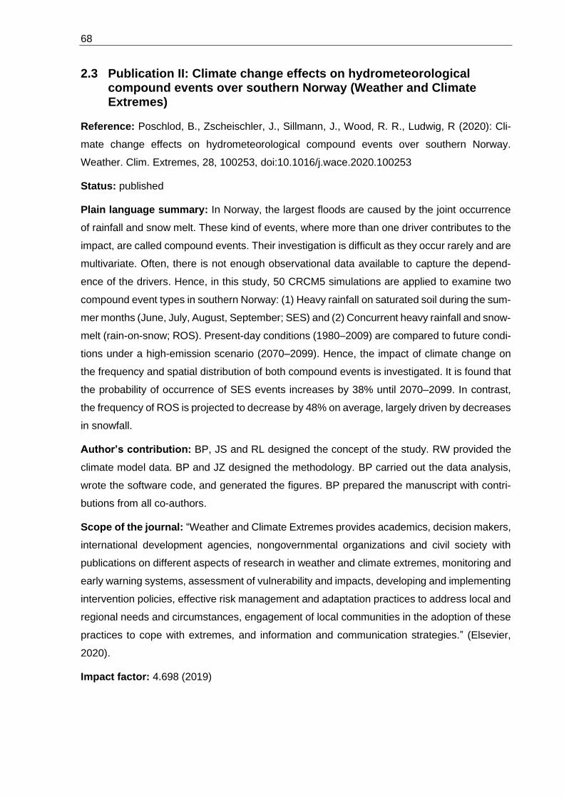
68

2.3 Publication II: Climate change effects on hydrometeorological compound events over southern Norway (Weather and Climate Extremes)

Reference: Poschlod, B., Zscheischler, J., Sillmann, J., Wood, R. R., Ludwig, R (2020): Cli-

mate change effects on hydrometeorological compound events over southern Norway.

Weather. Clim. Extremes, 28, 100253, doi:10.1016/j.wace.2020.100253

Status: published

Plain language summary: In Norway, the largest floods are caused by the joint occurrence

of rainfall and snow melt. These kind of events, where more than one driver contributes to the

impact, are called compound events. Their investigation is difficult as they occur rarely and are

multivariate. Often, there is not enough observational data available to capture the depend-

ence of the drivers. Hence, in this study, 50 CRCM5 simulations are applied to examine two

compound event types in southern Norway: (1) Heavy rainfall on saturated soil during the sum-

mer months (June, July, August, September; SES) and (2) Concurrent heavy rainfall and snow-

melt (rain-on-snow; ROS). Present-day conditions (1980–2009) are compared to future condi-

tions under a high-emission scenario (2070–2099). Hence, the impact of climate change on

the frequency and spatial distribution of both compound events is investigated. It is found that

the probability of occurrence of SES events increases by 38% until 2070–2099. In contrast,

the frequency of ROS is projected to decrease by 48% on average, largely driven by decreases

in snowfall.

Author’s contribution: BP, JS and RL designed the concept of the study. RW provided the

climate model data. BP and JZ designed the methodology. BP carried out the data analysis,

wrote the software code, and generated the figures. BP prepared the manuscript with contri-

butions from all co-authors.

Scope of the journal: “Weather and Climate Extremes provides academics, decision makers,

international development agencies, nongovernmental organizations and civil society with

publications on different aspects of research in weather and climate extremes, monitoring and

early warning systems, assessment of vulnerability and impacts, developing and implementing

intervention policies, effective risk management and adaptation practices to address local and

regional needs and circumstances, engagement of local communities in the adoption of these

practices to cope with extremes, and information and communication strategies.” (Elsevier,

2020).

Impact factor: 4.698 (2019)

Weather and Climate Extremes 28 (2020) 100253

Available online 18 March 20202212-0947/© 2020 The Authors. Published by Elsevier B.V. This is an open access article under the CC BY license (http://creativecommons.org/licenses/by/4.0/).

Climate change effects on hydrometeorological compound events over southern Norway

Benjamin Poschlod a,*, Jakob Zscheischler b,c, Jana Sillmann d, Raul R. Wood a, Ralf Ludwig a

a Department of Geography, Ludwig-Maximilians-University Munich, Luisenstr. 37, 80333, Munich, Germany b Climate and Environmental Physics, University of Bern, Sidlerstrasse 5, 3012, Bern, Switzerland c Oeschger Centre for Climate Change Research, University of Bern, 3012, Bern, Switzerland d Center for International Climate and Environmental Research (CICERO), Pb. 1129, Blindern, N-0318, Oslo, Norway

A R T I C L E I N F O

Keywords: Compound events Climate change Large ensemble Heavy rainfall Rain-on-snow Soil saturation Norway

A B S T R A C T

Hydrometeorological compound events cause severe economical, societal and environmental damage, but their investigation is difficult as they occur rarely and are multivariate. Here we use 50 high-resolution climate simulations from the single model initial condition large ensemble CRCM5-LE to examine two such compound event types in southern Norway: (1) Heavy rainfall on saturated soil during the summer months (June, July, August, September; SES) and (2) Concurrent heavy rainfall and snowmelt (rain-on-snow; ROS). We compare present-day conditions (1980–2009) with future conditions under a high-emission scenario (2070–2099) and investigate the impact of climate change on the frequency and spatial distribution of SES and ROS events. We find that the probability of occurrence of SES events during the summer increases by 38% until 2070–2099 over the whole study area. The areas with the highest occurrence probability extend from the west coast into the interior. In contrast, the frequency of ROS is projected to decrease by 48% on average, largely driven by de-creases in snowfall. Moreover, the spatial pattern of ROS are projected to change, with the most frequently affected areas shifting from the west coast towards the inner country. Our study highlights the benefits of single model large ensemble simulations for the analysis of compound events.

1. Introduction

A recent study of Berghuijs et al. (2019) has shown that most annual maximum floods in Europe are not caused by the highest annual rainfall peaks, but by the co-occurrence of rainfall and snowmelt or rainfall on saturated soil. These findings also hold for southern Norway as the combination of rainfall and snowmelt has resulted in the largest floods, for instance in south-eastern Norway in 1995 and 2013 (Krøgli et al., 2018). Concurrent heavy rainfall and snowmelt can also lead to several types of mass movements such as landslides, debris flow or slush flow. This type of event is often referred to as rain-on-snow (ROS) event. ROS events affect the local climate and hydrology by altering snowmelt, runoff, and soil temperatures and, therefore, it further affects vegeta-tion, wildlife and humans (Cohen et al., 2015; Putkonen and Roe, 2003). Seen globally, ROS events are a relatively rare phenomenon. However, they are often the main flood generating process in high latitudes (Cohen et al., 2015) and mountainous areas (McCabe et al., 2007; Merz and Bl€oschl, 2003). ROS events are therefore frequently found in the Arctic,

Scandinavia, Canada, Greenland and Spitsbergen (Putkonen and Roe, 2003). In Norway, ROS events typically occur during spring when the snow masses accumulated during the winter have not melted yet but temperature starts to rise (Benestad and Haugen, 2007; Pall et al., 2019).

Heavy rainfall on already saturated soil also regularly causes mass movements in southern Norway, such as landslides and flash floods (Dyrrdal et al., 2018). It leads to saturation excess surface runoff, which is often referred to as Dunne runoff (Zhenghui et al., 2003). In southern Norway, flood hazards and mass movements often severely impact infrastructure, economy, personal property, and may even cause fatal-ities (Krøgli et al., 2018).

ROS events and heavy rainfall on saturated soil are excellent exam-ples for compound events with often severe consequences. Compound events refer to the combination of multiple drivers and/or hazards that contributes to societal or environmental risk (Zscheischler et al., 2018). The individual contributing variables may not have to reach extreme values, but their joint occurrence may lead to a large impact (Bevacqua et al., 2017). The Intergovernmental Panel on Climate Change (IPCC)

* Corresponding author. E-mail address: Benjamin.Poschlod@lmu.de (B. Poschlod).

Contents lists available at ScienceDirect

Weather and Climate Extremes

journal homepage: http://www.elsevier.com/locate/wace

https://doi.org/10.1016/j.wace.2020.100253 Received 10 September 2019; Received in revised form 9 December 2019; Accepted 9 March 2020

Weather and Climate Extremes 28 (2020) 100253

2

has first introduced the term compound events within their Special Report on Managing the Risks of Extreme Events and Disasters to Advance Climate Change Adaptation, stressing the need to further explore the influence of climate change on compound events (Senevir-atne et al., 2012).

Compound events are rare and multivariate, and observational data only offer limited coverage and sparse sampling of the corners of a multidimensional space (Hao et al., 2018; Zscheischler et al., 2018). Hence, empirical analyses based on observational data are subject to substantial uncertainties due to the limited amount of available data. Conventional univariate statistical modeling is also not an appropriate method to study compound events, as long as there is any dependence between the contributing variables (Bevacqua et al., 2017; Wahl et al., 2015). Therefore, advanced multivariate methods are often applied to investigate the occurrence of compound events as the modeling of these events is complex (Leonard et al., 2014; Zscheischler and Seneviratne, 2017).

Copula theory and multivariate extreme value theory are frequently used to study compound events (Hao et al., 2018). These approaches can handle different types of dependencies between the contributing vari-ables of compound events and model them together with their marginal distributions (Bevacqua et al., 2017). Nevertheless, in many applications the sample size is very small (<< 1000), leading to large uncertainties (Serinaldi, 2013). To overcome the prevailing limitation of small sample sizes, ensembles of climate model simulations can be used to analyze compound events (van den Hurk et al., 2015; Zscheischler and Sen-eviratne, 2017).

Within this study, we use high-resolution climate simulations from the single model initial-condition large ensemble of the ClimEx project (www.climex-project.org) to investigate two different hydrometeoro-logical compound events in southern Norway and to explore the impact of a changing climate on these events: (1) Heavy rainfall on saturated soil during the summer months (June, July, August, September), which will be referred to as SES events (saturation excess during summer) and (2) Concurrent heavy rainfall and snowmelt, which will be referred to as ROS (rain-on-snow) events. The application of large ensembles of high- resolution climate simulations to study compound events is a relatively new approach (van den Hurk et al., 2015; Khanal et al., 2019; Zhou and Liu, 2018) even though they are ideally suited for this task due to their large sample size. The aim of this paper is to examine the probability of occurrence of SES and ROS events to map the spatial patterns and to evaluate the change between the reference period (1980–2009) and the far future (2070–2099) due to a changing climate under strong

greenhouse gas forcing.

2. Data and method

2.1. Study area

The study area covers southern Norway and parts of southwestern Sweden (Fig. 1a). The complex orography of the region is governed by the Scandinavian Mountains (or Langfjella) reaching from the northeast to the southwest (see Fig. 1b), whereas the western coastline is deeply indented by fjords. Southwestern Sweden shows little variation at low altitude.

Generally, three types of precipitation occur in southern Norway: (1) frontal, (2) orographic and (3) convective precipitation (Dyrrdal et al., 2016; Roe, 2005). The west coast is exposed to mainly large-scale frontal precipitation driven by the low pressure systems in the North Atlantic, which induce the biggest part of annual precipitation (Heikkil€a et al., 2011). Orography adds up to this, whereby the zone of maximum orographic precipitation is found 50 km inland (Sandvik et al., 2018; Tjelta and Mamen, 2014) with total annual precipitation above 3000 mm.

As these large weather systems mainly come from the west, the southeastern parts of the country are lee areas and the annual precipi-tation drops to 300–800 mm. Despite this, the highest hourly rainfall intensities occur in the region around the Oslofjord (Hanssen-Bauer et al., 2015). Convective showers and embedded convective cells within frontal systems can induce intensities of up to 40 mm/h with convection mainly occurring during the summer months from June to September (Dyrrdal et al., 2016; Poschlod et al., 2018). Hence, the precipitation amounts and intensities vary significantly within the study area depending on the types of precipitation systems and the orographic exposure.

The range in annual mean air temperature in southern Norway is mainly governed by the distance to the sea as well as the altitude (Hanssen-Bauer et al., 2015). Due to the heat content of the ocean, the mean temperatures are quite mild despite the high latitudes (Tjelta and Mamen, 2014). In southern Norway, they range from � 6 �C in the mountainous areas up to 8 �C at the coasts (Hanssen-Bauer et al., 2015). Soil moisture in southern Norway follows a weak seasonal cycle with averages around 0.3 m3/m3 (Pan et al., 2019) according to remote sensing products (ESA Soil Moisture CCI; Gruber et al., 2019) as well as reanalysis data (ERA-INTERIM; Dee et al., 2011). During winter and spring (December to May) soil moisture is slightly lower than in summer

Fig. 1. (a) Location of the study area over southern Norway. (b) Elevation of the study area.

B. Poschlod et al.

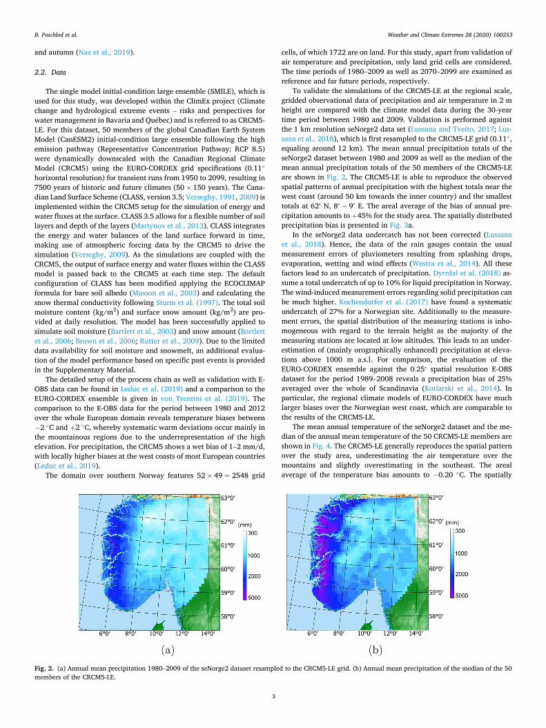
Weather and Climate Extremes 28 (2020) 100253

3

and autumn (Naz et al., 2019).

2.2. Data

The single model initial-condition large ensemble (SMILE), which is used for this study, was developed within the ClimEx project (Climate change and hydrological extreme events – risks and perspectives for water management in Bavaria and Qu�ebec) and is referred to as CRCM5- LE. For this dataset, 50 members of the global Canadian Earth System Model (CanESM2) initial-condition large ensemble following the high emission pathway (Representative Concentration Pathway: RCP 8.5) were dynamically downscaled with the Canadian Regional Climate Model (CRCM5) using the EURO-CORDEX grid specifications (0.11�

horizontal resolution) for transient runs from 1950 to 2099, resulting in 7500 years of historic and future climates (50� 150 years). The Cana-dian Land Surface Scheme (CLASS, version 3.5; Verseghy, 1991, 2009) is implemented within the CRCM5 setup for the simulation of energy and water fluxes at the surface. CLASS 3.5 allows for a flexible number of soil layers and depth of the layers (Martynov et al., 2013). CLASS integrates the energy and water balances of the land surface forward in time, making use of atmospheric forcing data by the CRCM5 to drive the simulation (Verseghy, 2009). As the simulations are coupled with the CRCM5, the output of surface energy and water fluxes within the CLASS model is passed back to the CRCM5 at each time step. The default configuration of CLASS has been modified applying the ECOCLIMAP formula for bare soil albedo (Masson et al., 2003) and calculating the snow thermal conductivity following Sturm et al. (1997). The total soil moisture content (kg/m2) and surface snow amount (kg/m2) are pro-vided at daily resolution. The model has been successfully applied to simulate soil moisture (Bartlett et al., 2003) and snow amount (Bartlett et al., 2006; Brown et al., 2006; Rutter et al., 2009). Due to the limited data availability for soil moisture and snowmelt, an additional evalua-tion of the model performance based on specific past events is provided in the Supplementary Material.

The detailed setup of the process chain as well as validation with E- OBS data can be found in Leduc et al. (2019) and a comparison to the EURO-CORDEX ensemble is given in von Trentini et al. (2019). The comparison to the E-OBS data for the period between 1980 and 2012 over the whole European domain reveals temperature biases between � 2 �C and þ2 �C, whereby systematic warm deviations occur mainly in the mountainous regions due to the underrepresentation of the high elevation. For precipitation, the CRCM5 shows a wet bias of 1–2 mm/d, with locally higher biases at the west coasts of most European countries (Leduc et al., 2019).

The domain over southern Norway features 52� 49 ¼ 2548 grid

cells, of which 1722 are on land. For this study, apart from validation of air temperature and precipitation, only land grid cells are considered. The time periods of 1980–2009 as well as 2070–2099 are examined as reference and far future periods, respectively.

To validate the simulations of the CRCM5-LE at the regional scale, gridded observational data of precipitation and air temperature in 2 m height are compared with the climate model data during the 30-year time period between 1980 and 2009. Validation is performed against the 1 km resolution seNorge2 data set (Lussana and Tveito, 2017; Lus-sana et al., 2018), which is first resampled to the CRCM5-LE grid (0.11�, equaling around 12 km). The mean annual precipitation totals of the seNorge2 dataset between 1980 and 2009 as well as the median of the mean annual precipitation totals of the 50 members of the CRCM5-LE are shown in Fig. 2. The CRCM5-LE is able to reproduce the observed spatial patterns of annual precipitation with the highest totals near the west coast (around 50 km towards the inner country) and the smallest totals at 62∘ N, 8∘ � 9∘ E. The areal average of the bias of annual pre-cipitation amounts to þ45% for the study area. The spatially distributed precipitation bias is presented in Fig. 3a.

In the seNorge2 data undercatch has not been corrected (Lussana et al., 2018). Hence, the data of the rain gauges contain the usual measurement errors of pluviometers resulting from splashing drops, evaporation, wetting and wind effects (Westra et al., 2014). All these factors lead to an undercatch of precipitation. Dyrrdal et al. (2018) as-sume a total undercatch of up to 10% for liquid precipitation in Norway. The wind-induced measurement errors regarding solid precipitation can be much higher. Kochendorfer et al. (2017) have found a systematic undercatch of 27% for a Norwegian site. Additionally to the measure-ment errors, the spatial distribution of the measuring stations is inho-mogeneous with regard to the terrain height as the majority of the measuring stations are located at low altitudes. This leads to an under-estimation of (mainly orographically enhanced) precipitation at eleva-tions above 1000 m a.s.l. For comparison, the evaluation of the EURO-CORDEX ensemble against the 0:25∘ spatial resolution E-OBS dataset for the period 1989–2008 reveals a precipitation bias of 25% averaged over the whole of Scandinavia (Kotlarski et al., 2014). In particular, the regional climate models of EURO-CORDEX have much larger biases over the Norwegian west coast, which are comparable to the results of the CRCM5-LE.

The mean annual temperature of the seNorge2 dataset and the me-dian of the annual mean temperature of the 50 CRCM5-LE members are shown in Fig. 4. The CRCM5-LE generally reproduces the spatial pattern over the study area, underestimating the air temperature over the mountains and slightly overestimating in the southeast. The areal average of the temperature bias amounts to � 0.20 �C. The spatially

Fig. 2. (a) Annual mean precipitation 1980–2009 of the seNorge2 dataset resampled to the CRCM5-LE grid. (b) Annual mean precipitation of the median of the 50 members of the CRCM5-LE.

B. Poschlod et al.

Weather and Climate Extremes 28 (2020) 100253

4

distributed bias is presented in Fig. 3b. For comparison, the evaluation of the EURO-CORDEX ensemble against the E-OBS data shows an annual temperature bias of � 0.35 �C over Scandinavia (Kotlarski et al., 2014). We conclude that the CRCM5-LE performs sufficiently well at repro-ducing the spatial distribution of precipitation and temperature and that the data are suitable for analyzing the southern Norwegian climate in more detail.

2.3. Methods

Because of the uncertainties due to the biases regarding precipitation and temperature, compound events in the CRCM5-LE cannot be defined by absolute thresholds derived from observations. The bias of precipi-tation and temperature can be corrected if the deviations are not caused by major model errors (Maraun et al., 2017), but would require multi-variate bias correction if compound events are to be captured adequately (Zscheischler et al., 2019). Furthermore, for this study, variables apart from precipitation and air temperature will be used, which cannot be bias corrected due to the lack of observations, for instance soil moisture and surface snow amount. We therefore apply a quantile-based approach to investigate the occurrence of compound events. Due to the very low compound exceedance of very high or low quantiles,

typically very long time series are required to obtain a sufficiently high number of events for robust statistical analysis (Zscheischler and Sen-eviratne, 2017). Here we have such conditions by using the CRCM5-LE with its 50 members, delivering a database of 1500 years of climate simulations for each 30-year period respectively.

We choose the 98th percentile P98 for each process contributing to the respective compound event based on the following considerations: The 98th percentile threshold includes the most extreme events in the far tail of the distribution, which are expected to cause the most severe damages, but it includes also relatively moderate extremes, which are impact-relevant as well (Martius et al., 2016; Zhang et al., 2011). Using the data from the CRCM5-LE, this threshold provides a sufficiently large number of samples for a robust statistical assessment of compound events (Sch€ar et al., 2016).

The P98 is calculated for each grid cell separately on the basis of the daily data and the respective time period including all 50 members of the CRCM5-LE. The daily sum of liquid precipitation is directly retrieved from the CRCM5-LE variable for each day d, whereas the soil moisture content of the previous day d � 1 is gathered from the CRCM5-LE to account for the soil state before the heavy precipitation event. Given that Norway is not in a dry or transitional climate, the soil is assumed to be very moist or saturated if P98 is exceeded. To estimate the amount of

Fig. 3. (a) Bias of the annual mean precipitation of the median of the 50 members of the CRCM5-LE compared to the seNorge2 dataset in 1980–2009. (b) Bias of the air temperature in 2 m height.

Fig. 4. (a) Annual mean air temperature in 2 m height 1980–2009 of the seNorge2 dataset resampled to the CRCM5-LE grid. (b) Annual mean air temperature of the median of the 50 members of the CRCM5-LE.

B. Poschlod et al.

Weather and Climate Extremes 28 (2020) 100253

5

melting snow for each grid cell at day d, we calculated the difference of surface snow amount on day d � 1 and dþ 1. We define two types of compound events. (1) The SES event is assumed to occur when liquid precipitation and soil moisture exceed their respective P98. (2) The occurrence of the ROS event is defined by liquid precipitation and snowmelt exceeding their respective P98. Being based on percentiles, the approach is insensitive to any bias in the variable means. The definition of ROS events based on a daily resolved analysis has also been applied by Musselman et al. (2018).

If both processes were independent, the probability of a simulta-neous occurrence would be 0.02 ⋅ 0.02 ¼ 0.0004, or 0:04%. In order to test whether both processes are significantly positively dependent, an independent reference dataset is created for each raster cell. For this, the values for one process variable (liquid precipitation) are randomly shuffled 1000 times and the occurrence probability for the compound event is calculated. A two-sample t-test with 1% significance level is then applied to test whether the re-sampled probability distribution and the original probability distribution of the CRCM5-LE 50 member ensemble originate from the same population. A statistical test with significance level α at n locations would yield n⋅α locations on average, where the null hypothesis is erroneously rejected, also called false positives

(Ventura et al., 2004). In our case, even the strict significance level of 1% would lead to 0:01⋅1722 ¼ 17:22 false positives on average. We there-fore correct the false discovery rate (FDR) (Benjamini and Hochberg, 1995) following Wilks (2016). More specifically, we reject H0 at all lo-cations i for which pi � pFDR, where

pFDR¼ maxi¼1;…;n

�

i : pðiÞ � αFDR ⋅�

in

��

;

with pðiÞ; i ¼ 1;…; n as the p-values of the statistical test sorted in ascending order, pð0Þ ¼ 0, and αFDR ¼ 2⋅α ¼ 0:02 (Ventura et al., 2004; Wilks, 2016). If the distributions do not originate from the same popu-lation and the average probability of occurrence in the CRCM5-LE is higher than in the independent reference data, it is assumed that both processes are positively dependent.

The comparison of the resulting probabilities of compound event occurrence between the present day and the far future period will be carried out in two ways: (1) The 98th percentile of the reference period (1980–2009) P98;ref is used as threshold for the future period and (2) the 98th percentile is re-calculated for the data of the future period (P98;fut). The latter variant is a “real” percentile-based method, whereas the first

Fig. 5. (a) Occurrence probability of SES events in the reference period 1980–2009 calculated with the median of the 50 members of the CRCM5-LE and applying P98;ref . Crosses denote regions where the underlying processes are significantly positively dependent (pi � pFDR). (b) Occurrence probability of SES events in the far future period 2070–2099 calculated with the median of the 50 members of the CRCM5-LE and applying P98;ref . (c) Change of the occurrence probability of SES events between the reference period and far future period. Crosses denote regions where the change is significant (pi � pFDR). (d) Occurrence probability of SES events the far future period 2070–2099 calculated with the median of the 50 members of the CRCM5-LE and applying P98;fut . Crosses denote regions where the underlying processes are significantly positively dependent (pi � pFDR).

B. Poschlod et al.

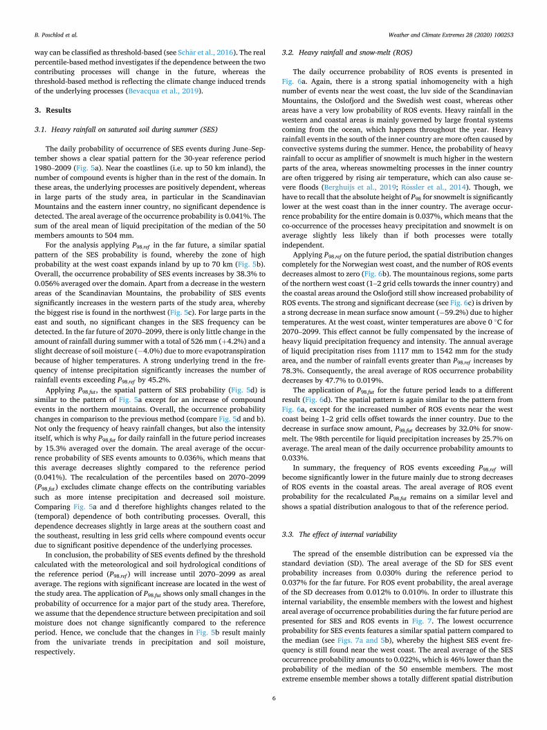
Weather and Climate Extremes 28 (2020) 100253

6

way can be classified as threshold-based (see Sch€ar et al., 2016). The real percentile-based method investigates if the dependence between the two contributing processes will change in the future, whereas the threshold-based method is reflecting the climate change induced trends of the underlying processes (Bevacqua et al., 2019).

3. Results

3.1. Heavy rainfall on saturated soil during summer (SES)

The daily probability of occurrence of SES events during June–Sep-tember shows a clear spatial pattern for the 30-year reference period 1980–2009 (Fig. 5a). Near the coastlines (i.e. up to 50 km inland), the number of compound events is higher than in the rest of the domain. In these areas, the underlying processes are positively dependent, whereas in large parts of the study area, in particular in the Scandinavian Mountains and the eastern inner country, no significant dependence is detected. The areal average of the occurrence probability is 0.041%. The sum of the areal mean of liquid precipitation of the median of the 50 members amounts to 504 mm.

For the analysis applying P98;ref in the far future, a similar spatial pattern of the SES probability is found, whereby the zone of high probability at the west coast expands inland by up to 70 km (Fig. 5b). Overall, the occurrence probability of SES events increases by 38.3% to 0.056% averaged over the domain. Apart from a decrease in the western areas of the Scandinavian Mountains, the probability of SES events significantly increases in the western parts of the study area, whereby the biggest rise is found in the northwest (Fig. 5c). For large parts in the east and south, no significant changes in the SES frequency can be detected. In the far future of 2070–2099, there is only little change in the amount of rainfall during summer with a total of 526 mm (þ4.2%) and a slight decrease of soil moisture (� 4.0%) due to more evapotranspiration because of higher temperatures. A strong underlying trend in the fre-quency of intense precipitation significantly increases the number of rainfall events exceeding P98;ref by 45.2%.

Applying P98;fut , the spatial pattern of SES probability (Fig. 5d) is similar to the pattern of Fig. 5a except for an increase of compound events in the northern mountains. Overall, the occurrence probability changes in comparison to the previous method (compare Fig. 5d and b). Not only the frequency of heavy rainfall changes, but also the intensity itself, which is why P98;fut for daily rainfall in the future period increases by 15.3% averaged over the domain. The areal average of the occur-rence probability of SES events amounts to 0.036%, which means that this average decreases slightly compared to the reference period (0.041%). The recalculation of the percentiles based on 2070–2099 (P98;fut) excludes climate change effects on the contributing variables such as more intense precipitation and decreased soil moisture. Comparing Fig. 5a and d therefore highlights changes related to the (temporal) dependence of both contributing processes. Overall, this dependence decreases slightly in large areas at the southern coast and the southeast, resulting in less grid cells where compound events occur due to significant positive dependence of the underlying processes.

In conclusion, the probability of SES events defined by the threshold calculated with the meteorological and soil hydrological conditions of the reference period (P98;ref ) will increase until 2070–2099 as areal average. The regions with significant increase are located in the west of the study area. The application of P98;fut shows only small changes in the probability of occurrence for a major part of the study area. Therefore, we assume that the dependence structure between precipitation and soil moisture does not change significantly compared to the reference period. Hence, we conclude that the changes in Fig. 5b result mainly from the univariate trends in precipitation and soil moisture, respectively.

3.2. Heavy rainfall and snow-melt (ROS)

The daily occurrence probability of ROS events is presented in Fig. 6a. Again, there is a strong spatial inhomogeneity with a high number of events near the west coast, the luv side of the Scandinavian Mountains, the Oslofjord and the Swedish west coast, whereas other areas have a very low probability of ROS events. Heavy rainfall in the western and coastal areas is mainly governed by large frontal systems coming from the ocean, which happens throughout the year. Heavy rainfall events in the south of the inner country are more often caused by convective systems during the summer. Hence, the probability of heavy rainfall to occur as amplifier of snowmelt is much higher in the western parts of the area, whereas snowmelting processes in the inner country are often triggered by rising air temperature, which can also cause se-vere floods (Berghuijs et al., 2019; R€ossler et al., 2014). Though, we have to recall that the absolute height of P98 for snowmelt is significantly lower at the west coast than in the inner country. The average occur-rence probability for the entire domain is 0.037%, which means that the co-occurrence of the processes heavy precipitation and snowmelt is on average slightly less likely than if both processes were totally independent.

Applying P98;ref on the future period, the spatial distribution changes completely for the Norwegian west coast, and the number of ROS events decreases almost to zero (Fig. 6b). The mountainous regions, some parts of the northern west coast (1–2 grid cells towards the inner country) and the coastal areas around the Oslofjord still show increased probability of ROS events. The strong and significant decrease (see Fig. 6c) is driven by a strong decrease in mean surface snow amount (� 59.2%) due to higher temperatures. At the west coast, winter temperatures are above 0 �C for 2070–2099. This effect cannot be fully compensated by the increase of heavy liquid precipitation frequency and intensity. The annual average of liquid precipitation rises from 1117 mm to 1542 mm for the study area, and the number of rainfall events greater than P98;ref increases by 78.3%. Consequently, the areal average of ROS occurrence probability decreases by 47.7% to 0.019%.

The application of P98;fut for the future period leads to a different result (Fig. 6d). The spatial pattern is again similar to the pattern from Fig. 6a, except for the increased number of ROS events near the west coast being 1–2 grid cells offset towards the inner country. Due to the decrease in surface snow amount, P98;fut decreases by 32.0% for snow-melt. The 98th percentile for liquid precipitation increases by 25.7% on average. The areal mean of the daily occurrence probability amounts to 0.033%.

In summary, the frequency of ROS events exceeding P98;ref will become significantly lower in the future mainly due to strong decreases of ROS events in the coastal areas. The areal average of ROS event probability for the recalculated P98;fut remains on a similar level and shows a spatial distribution analogous to that of the reference period.

3.3. The effect of internal variability

The spread of the ensemble distribution can be expressed via the standard deviation (SD). The areal average of the SD for SES event probability increases from 0.030% during the reference period to 0.037% for the far future. For ROS event probability, the areal average of the SD decreases from 0.012% to 0.010%. In order to illustrate this internal variability, the ensemble members with the lowest and highest areal average of occurrence probabilities during the far future period are presented for SES and ROS events in Fig. 7. The lowest occurrence probability for SES events features a similar spatial pattern compared to the median (see Figs. 7a and 5b), whereby the highest SES event fre-quency is still found near the west coast. The areal average of the SES occurrence probability amounts to 0.022%, which is 46% lower than the probability of the median of the 50 ensemble members. The most extreme ensemble member shows a totally different spatial distribution

B. Poschlod et al.

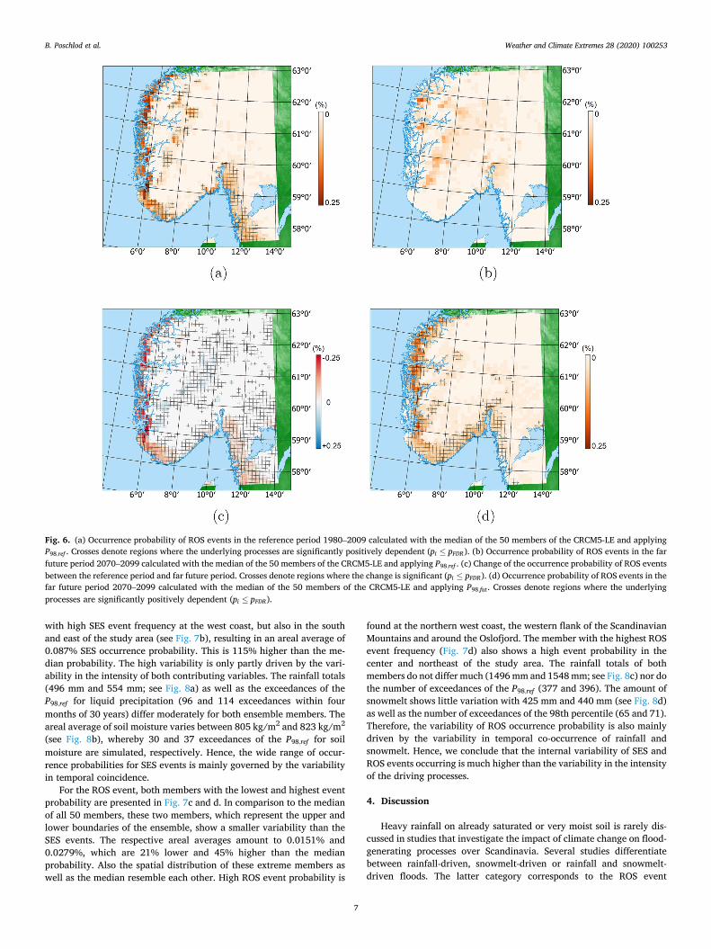
Weather and Climate Extremes 28 (2020) 100253

7

with high SES event frequency at the west coast, but also in the south and east of the study area (see Fig. 7b), resulting in an areal average of 0.087% SES occurrence probability. This is 115% higher than the me-dian probability. The high variability is only partly driven by the vari-ability in the intensity of both contributing variables. The rainfall totals (496 mm and 554 mm; see Fig. 8a) as well as the exceedances of the P98;ref for liquid precipitation (96 and 114 exceedances within four months of 30 years) differ moderately for both ensemble members. The areal average of soil moisture varies between 805 kg/m2 and 823 kg/m2

(see Fig. 8b), whereby 30 and 37 exceedances of the P98;ref for soil moisture are simulated, respectively. Hence, the wide range of occur-rence probabilities for SES events is mainly governed by the variability in temporal coincidence.

For the ROS event, both members with the lowest and highest event probability are presented in Fig. 7c and d. In comparison to the median of all 50 members, these two members, which represent the upper and lower boundaries of the ensemble, show a smaller variability than the SES events. The respective areal averages amount to 0.0151% and 0.0279%, which are 21% lower and 45% higher than the median probability. Also the spatial distribution of these extreme members as well as the median resemble each other. High ROS event probability is

found at the northern west coast, the western flank of the Scandinavian Mountains and around the Oslofjord. The member with the highest ROS event frequency (Fig. 7d) also shows a high event probability in the center and northeast of the study area. The rainfall totals of both members do not differ much (1496 mm and 1548 mm; see Fig. 8c) nor do the number of exceedances of the P98;ref (377 and 396). The amount of snowmelt shows little variation with 425 mm and 440 mm (see Fig. 8d) as well as the number of exceedances of the 98th percentile (65 and 71). Therefore, the variability of ROS occurrence probability is also mainly driven by the variability in temporal co-occurrence of rainfall and snowmelt. Hence, we conclude that the internal variability of SES and ROS events occurring is much higher than the variability in the intensity of the driving processes.

4. Discussion

Heavy rainfall on already saturated or very moist soil is rarely dis-cussed in studies that investigate the impact of climate change on flood- generating processes over Scandinavia. Several studies differentiate between rainfall-driven, snowmelt-driven or rainfall and snowmelt- driven floods. The latter category corresponds to the ROS event

Fig. 6. (a) Occurrence probability of ROS events in the reference period 1980–2009 calculated with the median of the 50 members of the CRCM5-LE and applying P98;ref . Crosses denote regions where the underlying processes are significantly positively dependent (pi � pFDR). (b) Occurrence probability of ROS events in the far future period 2070–2099 calculated with the median of the 50 members of the CRCM5-LE and applying P98;ref . (c) Change of the occurrence probability of ROS events between the reference period and far future period. Crosses denote regions where the change is significant (pi � pFDR). (d) Occurrence probability of ROS events in the far future period 2070–2099 calculated with the median of the 50 members of the CRCM5-LE and applying P98;fut . Crosses denote regions where the underlying processes are significantly positively dependent (pi � pFDR).

B. Poschlod et al.

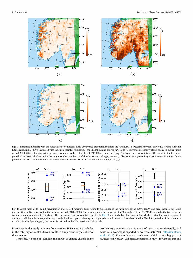
Weather and Climate Extremes 28 (2020) 100253

8

introduced in this study, whereas flood-causing SES events are included in the category of rainfall-driven events, but represent only a subset of these events.

Therefore, we can only compare the impact of climate change on the

two driving processes to the outcome of other studies. Generally, soil moisture in Norway is expected to decrease until 2100 (Hanssen-Bauer et al., 2015). For the Glomma catchment, which covers big parts of southeastern Norway, soil moisture during 15 May - 15 October is found

Fig. 7. Ensemble members with the most extreme compound event occurrence probabilities during the far future. (a) Occurrence probability of SES events in the far future period 2070–2099 calculated with the single member number 3 of the CRCM5-LE and applying P98;ref . (b) Occurrence probability of SES events in the far future period 2070–2099 calculated with the single member number 11 of the CRCM5-LE and applying P98;ref . (c) Occurrence probability of ROS events in the far future period 2070–2099 calculated with the single member number 21 of the CRCM5-LE and applying P98;ref . (d) Occurrence probability of ROS events in the far future period 2070–2099 calculated with the single member number 48 of the CRCM5-LE and applying P98;ref .

Fig. 8. Areal mean of (a) liquid precipitation and (b) soil moisture during June to September of the far future period (2070–2099) and areal mean of (c) liquid precipitation and (d) snowmelt of the far future period (2070–2099). The boxplots show the range over the 50 members of the CRCM5-LE, whereby the two members with maximum/minimum SES (a,b) and ROS (c,d) occurrence probability, respectively (Fig. 7), are marked as blue squares. The whiskers extend up to a maximum of one and a half times the interquartile range, and all values beyond this range are regarded as outliers (marked as a black circle). (For interpretation of the references to colour in this figure legend, the reader is referred to the Web version of this article.)

B. Poschlod et al.

Weather and Climate Extremes 28 (2020) 100253

9

to decrease moderately until 2070–2099, whereby precipitation stays on a similar level (Wong et al., 2011). This experiment was carried out using two different GCMs (ECHAM4 and HadCM3) under the Special Report on Emissions Scenarios (SRES) A2 and B2. The change of rainfall totals during June, July and August over southern Norway is estimated to be between � 5% and þ15% within the EURO-CORDEX ensemble under the RCP 8.5 scenario, whereby heavy precipitation is found to increase by 15–25% (Jacob et al., 2014). These findings regarding soil moisture and precipitation during summer are consistent with the trends discovered in this study.

Regarding the change of ROS event frequency until the far future under RCP 8.5, similar results have been found for other mountainous regions, for instance by Musselman et al. (2018) for western North America. They discovered a significant decrease of ROS event frequency at coastal areas and lower elevations due to snowpack declines. At higher elevations with seasonally persisting snowcover, ROS is found to become more frequent due to a shift from snowfall to rain. Though, their study applies lower thresholds to define ROS events with rainfall greater than 10 mm/d and snowmelt greater than 2 mm/d. Benestad and Haugen (2007) investigated the occurrence of heavy rainfall together with snowmelt in Norway based on 50 km resolution HIRHAM simula-tions from 1980 to 1999 and 2030–2049. They focused only on spring time temperature and precipitation and assumed the snow amount to be constant between the two time periods. They found that spring time floods due to concurrent rainfall and snowmelt will increase in the future because of rising temperatures and increasing spring-time pre-cipitation. We also find rising temperatures and precipitation during spring, but our findings regarding ROS events challenge the results of Benestad and Haugen (2007) since a stable surface snow amount is an unrealistic assumption with continuous warming. In the CRCM5-LE, the mean snow surface amount averaged over the study area until 2070–2099 decreases by 59.2% in comparison to 1980–2009 for the median of the 50 ensemble members.

Also, Pall et al. (2019) find a negative trend of ROS event frequency in historical observational data (1961–2010), whereby Vormoor et al. (2016) state that the importance of snowmelt as flood driver decreased between 1962 and 2012. This trend is found to continue within the CRCM5-LE simulations, as the areal average of the ratio of P98 of snowmelt divided by P98 of liquid precipitation almost decreases to half (Fig. 9). Several hydrological studies report the decreasing importance of snowmelt as flood driver in the far future as well, whereas increasing rainfall totals and intensities lead to higher flood magnitudes in rainfall-driven catchments (Lawrence and Hisdal, 2011; Madsen et al., 2014; Rojas et al., 2012; Vormoor et al., 2015). Therefore, our findings

regarding future trends tie in with the results of these studies on past, present and future climate change induced trends.

In our analysis, the ROS and SES events are defined by the respective meteorological and hydrological drivers exceeding the 98th percentile. Zscheischler et al. (2018) propose that the investigation of compound events should focus on the impact rather than on the drivers, which would mean in our case that the change in frequency, intensity and extent of the floods resulting from ROS and SES events should be assessed. Implementing this focus within the framework of SMILE is a computationally expensive and labor-intensive task. Although out of scope for the present study, within the ClimEx project, it is planned to apply bias adjustment and further spatial downscaling to all 50 members of the climate simulations of the CRCM5-LE in order to run a hydro-logical impact model over Bavaria and Qu�ebec (Leduc et al., 2019).

As with all analyses based on climate simulations, there are un-certainties within this study as well. Generally, the overall uncertainty of climate projections can be addressed to three different sources: (1) scenario uncertainty arising from the fact that future emissions are un-known, (2) model or response uncertainty, as different models yield different climate simulations though driven by the same radiative forcing and (3) internal or natural variability, which is caused by non- linear dynamical processes intrinsic to the atmosphere (Deser et al., 2012; Hawkins and Sutton, 2009; von Trentini et al., 2019). A SMILE such as the CRCM5-LE does not address scenario or model/response uncertainties as only one set of global circulation model (GCM: Can-ESM2), regional climate model (RCM: CRCM5) and emission pathway (RCP 8.5) is used (Leduc et al., 2019). Nonetheless, the large ensemble size of 50 members offers a broad database of 50 equally probable climate simulations, which differ only due to the internal variability of the climate system (Deser et al., 2012). This enables a robust estimate of the occurrence probability of very rare events such as compound events under the assumptions of the chosen emission scenario and the model-internal representation of the physical processes within the RCM and GCM. Though one has to keep in mind that the numerical analysis of occurrence probabilities in section 3 is based on the median representing only the center of the ensemble, whereas single members at the edges of the ensemble distribution feature more extreme scenarios.

To better understand the role of internal variability and also extreme events in current climate projections, several SMILE experiments were set up in the last years (Leduc et al., 2019; Aalbers et al., 2018; Addor and Fischer, 2015). They are a particularly powerful tool for the inves-tigation of compound events. Continuous advances in computational speed allow to run an unprecedented size of ensemble members. For instance, the simulations of the Grand Ensemble of the MPI-ESM have

Fig. 9. (a) Ratio of the P98;ref of snowmelt/ P98;ref of liquid precipitation for the reference period as relative indicator for the importance as flood driver (Fassnacht and Records, 2015) (b) Ratio of the P98;fut of snowmelt/ P98;fut of liquid precipitation for the far future period.

B. Poschlod et al.

Weather and Climate Extremes 28 (2020) 100253

10

been recently completed, which include 100 ensemble members for the historical time period and four different emission scenarios (Maher et al., 2019). Therefore, scenario uncertainty can be addressed in addition to the internal variability of the 100 members though the broader spatial resolution of GCMs is not suitable for research questions that relate to features of a regional climate and topography (Giorgi et al., 2016; Prein et al., 2016). The dynamical downscaling of the CanESM2 runs by CRCM5-LE with a final resolution of 0.11� allows a represen-tation of the topography to map mesoscale processes such as orographic precipitation. Especially for the complex topography and different pre-cipitation types over Scandinavia, Heikkil€a et al. (2011) and Mayer et al. (2015) emphasize the value added by dynamical downscaling and spatial resolutions of 10 km and 8 km, respectively. Though, even higher resolutions are recommended by Barstad and Caroletti (2013) and Poschlod et al. (2018) to recreate topographical features on a local scale and explicitly resolve convectional processes. Within the CRCM5-LE convection is parameterized as the physical processes leading to shallow convection can only sufficiently be resolved at resolutions of 4 km or less (Prein et al., 2015; Tabari et al., 2016).

5. Conclusion

We apply a quantile-based analysis on two compound events (heavy rainfall on saturated soil during summer (SES) and concurrent heavy rainfall and snowmelt (ROS)) in southern Norway using data from the single model initial condition large ensemble CRCM5-LE. This analysis illustrates the impact of a changing climate on the frequency and spatial distribution of those events. The occurrence probability of heavy rainfall events on very moist soil increases by 38% from 1980 to 2009 to 2070–2099, whereas the frequency of ROS events decreases by 48% for the whole study area in a high emission scenario (RCP 8.5). Applying a regional climate model large ensemble with 0.11� resolution enables the representation of topographical features and investigation of (hydro-) meteorological processes at finer spatial scales than are typically avail-able in global climate models. Hence, spatial patterns and in-homogeneity relating to regional features and processes could be mapped. The regions with high occurrence probability for SES events are located at the Norwegian west coast. Until 2070–2099, these regions expand towards the inner country, whereby the zone with the highest probability is found in the northwest. Despite the strong decrease in ROS event probability over most of the study region due to a reduction in snowfall, there are still areas of high event frequency in the far future. These areas are located mainly on the western flanks of the Scandinavian Mountains, but also at the northwestern coast and around the Oslofjord. The importance of these three drivers of compound floods will shift towards a flood regime less governed by snowmelt, but increasingly triggered by heavy rainfall and saturation excess. Using a large ensemble with 50 members leads to a sufficiently high number of events with very rare occurrence probabilities. Therefore, the analysis results in statisti-cally robust estimations of event probabilities and alterations of these probabilities due to climate change. We show that for single ensemble members, the occurrence probabilities of especially SES events, but also ROS events vary greatly. We attribute this variation to the variability in the timing of the co-occurrence of the contributing processes, which is found to be governed by the internal variability of the climate system. Therefore, a large ensemble size is required to assess the occurrence probability. A similar approach can be applied to examine other types of compound events and how climate change affects their occurrence.

Declaration of competing interest

The authors declare that they have no known competing financial interests or personal relationships that could have appeared to influence the work reported in this paper.

CRediT authorship contribution statement

Benjamin Poschlod: Conceptualization, Methodology, Formal analysis, Software, Visualization, Writing - original draft, Writing - re-view & editing. Jakob Zscheischler: Writing - review & editing, Methodology, Funding acquisition. Jana Sillmann: Writing - review & editing, Conceptualization, Project administration. Raul R. Wood: Writing - review & editing, Resources. Ralf Ludwig: Writing - review & editing, Conceptualization, Supervision, Funding acquisition.

Acknowledgement

We thank all members of the ClimEx project working group for their contributions to produce and analyze the CanESM2-LE and CRCM5-LE. The ClimEx project is funded by the Bavarian State Ministry of the Environment and Consumer Protection. The CRCM5 was developed by the ESCER centre of Universit�e du Qu�ebec a Montr�eal (UQAM; http: //www.escer.uqam.ca) in collaboration with Environment and Climate Change Canada. We thank the Canadian Centre for Climate Modelling and Analysis (CCCma) for executing and making available the CanESM2 Large Ensemble simulations used in this study, and the Ca-nadian Sea Ice and Snow Evolution (CanSISE) Network for proposing the simulations. Computations with the CRCM5 for the ClimEx project were made on the SuperMUC supercomputer at Leibniz Supercomputing Centre (LRZ) of the Bavarian Academy of Sciences and Humanities. The operation of this supercomputer is funded via the Gauss Centre for Supercomputing (GCS) by the German Federal Ministry of Education and Research and the Bavarian State Ministry of Education, Science and the Arts. Additionally, we acknowledge the European COST Action DAMOCLES (CA17109) which supported a Short-Term Scientific Mission of BP at CICERO in Oslo, which contributed significantly to the conception of this study. JZ acknowledges funding from the Swiss Na-tional Science Foundation (Ambizione grant 179876). JS is supported by the Norwegian Research Council funded project TWEX (Grant nr. 255037).

Appendix A. Supplementary data

Supplementary data to this article can be found online at https://doi. org/10.1016/j.wace.2020.100253.

References

Aalbers, E.E., Lenderink, G., van Meijgaard, E., van den Hurk, B.J.J.M., 2018. Local-scale changes in mean and heavy precipitation in western Europe, climate change or internal variability? Clim. Dynam. 50, 4745–4766. https://doi.org/10.1007/s00382- 017-3901-9.

Addor, N., Fischer, E.M., 2015. The influence of natural variability and interpolation errors on bias characterization in RCM simulations. J. Geophys. Res.: Atmosphere 120, 10180–10195. https://doi.org/10.1002/2014JD022824.

Barstad, I., Caroletti, G., 2013. Orographic precipitation across an island in southern Norway: model evaluation of time-step precipitation. Q. J. R. Meteorol. Soc. 139, 1555–1565. https://doi.org/10.1002/qj.2067.

Bartlett, P.A., Harry McCaughey, J., Lafleur, P.M., Verseghy, D.L., 2003. Modelling evapotranspiration at three boreal forest stands using the CLASS: tests of parameterizations for canopy conductance and soil evaporation. Int. J. Climatol. 23, 427–451. https://doi.org/10.1002/joc.884.

Bartlett, P.A., MacKay, M.D., Verseghy, D.L., 2006. Modified snow algorithms in the Canadian land surface scheme: model runs and sensitivity analysis at three boreal forest stands. Atmos.-Ocean 44, 207–222. https://doi.org/10.3137/ao.440301.

Benestad, R.E., Haugen, J.E., 2007. On complex extremes: flood hazards and combined high spring-time precipitation and temperature in Norway. Climatic Change 85, 381–406. https://doi.org/10.1007/s10584-007-9263-2.

Benjamini, Y., Hochberg, Y., 1995. Controlling the false discovery rate - a practical and powerful approach to multiple testing. J. Roy. Stat. Soc. B 57, 289–300. https://doi. org/10.2307/2346101.

Berghuijs, W.R., Harrigan, S., Molnar, P., Slater, L.J., Kirchner, J.W., 2019. The relative importance of different flood-generating mechanisms across Europe. Water Resour. Res. 55, 4582–4593. https://doi.org/10.1029/2019WR024841.

Bevacqua, E., Maraun, D., Hobæk Haff, I., Widmann, M., Vrac, M., 2017. Multivariate statistical modelling of compound events via pair-copula constructions: analysis of floods in Ravenna (Italy). Hydrol. Earth Syst. Sci. 21, 2701–2723. https://doi.org/ 10.5194/hess-21-2701-2017.

B. Poschlod et al.

Weather and Climate Extremes 28 (2020) 100253

11

Bevacqua, E., Maraun, D., Vousdoukas, M., Voukouvalas, E., Vrac, M., Mentaschi, L., Widmann, M., 2019. Higher potential compound flood risk in northern Europe under anthropogenic climate change. Sci. Adv. 5 https://doi.org/10.1126/sciadv. aaw5531.

Brown, R., Bartlett, P., MacKay, M., Verseghy, D., 2006. Evaluation of snow cover in CLASS for SnowMIP. Atmos.-Ocean 44, 223–238. https://doi.org/10.3137/ ao.440302.

Cohen, J., Ye, H., Jones, J., 2015. Trends and variability in rain-on-snow events. Geophys. Res. Lett. 42, 7115–7122. https://doi.org/10.1002/2015GL065320.

Dee, D.P., Uppala, S.M., Simmons, A.J., Berrisford, P., Poli, P., Kobayashi, S., Andrae, U., Balmaseda, M.A., Balsamo, G., Bauer, P., Bechtold, P., Beljaars, A.C.M., van de Berg, L., Bidlot, J., Bormann, N., Delsol, C., Dragani, R., Fuentes, M., Geer, A.J., Haimberger, L., Healy, S.B., Hersbach, H., H�olm, E.V., Isaksen, L., Kållberg, P., K€ohler, M., Matricardi, M., McNally, A.P., Monge-Sanz, B.M., Morcrette, J.J., Park, B.K., Peubey, C., de Rosnay, P., Tavolato, C., Th�epaut, J.N., Vitart, F., 2011. The ERA-Interim reanalysis: configuration and performance of the data assimilation system. Q. J. R. Meteorol. Soc. 137, 553–597. https://doi.org/10.1002/qj.828.

Deser, C., Phillips, A., Bourdette, V., Teng, H., 2012. Uncertainty in climate change projections: the role of internal variability. Clim. Dynam. 38, 527–546. https://doi. org/10.1007/s00382-010-0977-x.

Dyrrdal, A.V., Skaugen, T., Stordal, F., Førland, E.J., 2016. Estimating extreme areal precipitation in Norway from a gridded dataset. Hydrol. Sci. J. 61, 483–494. https:// doi.org/10.1080/02626667.2014.947289.

Dyrrdal, A.V., Stordal, F., Lussana, C., 2018. Evaluation of summer precipitation from EURO-CORDEX fine-scale RCM simulations over Norway. Int. J. Climatol. 38, 1661–1677. https://doi.org/10.1002/joc.5287.

Fassnacht, S.R., Records, R.M., 2015. Large snowmelt versus rainfall events in the mountains. J. Geophys. Res.: Atmosphere 120, 2375–2381. https://doi.org/ 10.1002/2014JD022753.

Giorgi, F., Torma, C., Coppola, E., Ban, N., Sch€ar, C., Somot, S., 2016. Enhanced summer convective rainfall at alpine high elevations in response to climate warming. Nat. Geosci. 9, 584–589. https://doi.org/10.1038/ngeo2761.

Gruber, A., Scanlon, T., van der Schalie, R., Wagner, W., Dorigo, W., 2019. Evolution of the ESA CCI Soil Moisture climate data records and their underlying merging methodology. Earth Syst. Sci. Data 11, 717–739. https://doi.org/10.5194/essd-11- 717-2019.

Hanssen-Bauer, I., Drange, H., Førland, E.J., Roald, L.A., Børsheim, K.Y., Hisdal, H., Mayer, S., Nesje, A., Nilsen, J.E.Ø., Sandven, S., Sandø, A.B., Sorteberg, A., Ådlandsvik, B., 2015. Klima I Norge 2100. Kunnskapsgrunnlag for Klimatilpasning Oppdatert I 2015. Technical Report. Norsk klimaservicesenter, Oslo, Norway.

Hao, Z., Singh, V.P., Hao, F., 2018. Compound extremes in hydroclimatology: a review. Water 10. https://doi.org/10.3390/w10060718.

Hawkins, E., Sutton, R., 2009. The potential to narrow uncertainty in regional climate predictions. Bull. Am. Meteorol. Soc. 90, 1095–1108. https://doi.org/10.1175/ 2009BAMS2607.1.

Heikkil€a, U., Sandvik, A., Sorteberg, A., 2011. Dynamical downscaling of ERA-40 in complex terrain using the WRF regional climate model. Clim. Dynam. 37, 1551–1564. https://doi.org/10.1007/s00382-010-0928-6.

van den Hurk, B., van Meijgaard, E., de Valk, P., van Heeringen, K.J., Gooijer, J., 2015. Analysis of a compounding surge and precipitation event in The Netherlands. Environ. Res. Lett. 10, 035001 https://doi.org/10.1088/1748-9326/10/3/035001.

Jacob, D., Petersen, J., Eggert, B., Alias, A., Christensen, O.B., Bouwer, L.M., Braun, A., Colette, A., D�equ�e, M., Georgievski, G., Georgopoulou, E., Gobiet, A., Menut, L., Nikulin, G., Haensler, A., Hempelmann, N., Jones, C., Keuler, K., Kovats, S., Kr€oner, N., Kotlarski, S., Kriegsmann, A., Martin, E., van Meijgaard, E., Moseley, C., Pfeifer, S., Preuschmann, S., Radermacher, C., Radtke, K., Rechid, D., Rounsevell, M., Samuelsson, P., Somot, S., Soussana, J.F., Teichmann, C., Valentini, R., Vautard, R., Weber, B., Yiou, P., 2014. EURO-CORDEX: new high- resolution climate change projections for European impact research. Reg. Environ. Change 14, 563–578. https://doi.org/10.1007/s10113-013-0499-2.

Khanal, S., Lutz, A.F., Immerzeel, W.W., Vries, H.d., Wanders, N., Hurk, B.v.d., 2019. The impact of meteorological and hydrological memory on compound peak flows in the Rhine river basin. Atmosphere 10. https://doi.org/10.3390/atmos10040171.

Kochendorfer, J., Rasmussen, R., Wolff, M., Baker, B., Hall, M.E., Meyers, T., Landolt, S., Jachcik, A., Isaksen, K., Brækkan, R., Leeper, R., 2017. The quantification and correction of wind-induced precipitation measurement errors. Hydrol. Earth Syst. Sci. 21, 1973–1989. https://doi.org/10.5194/hess-21-1973-2017.

Kotlarski, S., Keuler, K., Christensen, O.B., Colette, A., D�equ�e, M., Gobiet, A., Goergen, K., Jacob, D., Lüthi, D., van Meijgaard, E., Nikulin, G., Sch€ar, C., Teichmann, C., Vautard, R., Warrach-Sagi, K., Wulfmeyer, V., 2014. Regional climate modeling on European scales: a joint standard evaluation of the EURO- CORDEX RCM ensemble. Geosci. Model Dev. (GMD) 7, 1297–1333. https://doi.org/ 10.5194/gmd-7-1297-2014.

Krøgli, I.K., Devoli, G., Colleuille, H., Boje, S., Sund, M., Engen, I.K., 2018. The Norwegian forecasting and warning service for rainfall- and snowmelt-induced landslides. Nat. Hazards Earth Syst. Sci. 18, 1427–1450. https://doi.org/10.5194/ nhess-18-1427-2018.

Lawrence, D., Hisdal, H., 2011. Hydrological Projections for Floods in Norway under a Future Climate. Technical Report 5. Norwegian Water Resources and Energy Directorate, Oslo, Norway.

Leduc, M., Mailhot, A., Frigon, A., Martel, J.L., Ludwig, R., Brietzke, G.B., Gigu�ere, M., Brissette, F., Turcotte, R., Braun, M., Scinocca, J., 2019. The ClimEx project: a 50- member ensemble of climate change projections at 12-km resolution over Europe and northeastern north America with the Canadian regional climate model (CRCM5). J. Appl. Meteorol. Climatol. 58, 663–693. https://doi.org/10.1175/ JAMC-D-18-0021.1.

Leonard, M., Westra, S., Phatak, A., Lambert, M., van den Hurk, B., McInnes, K., Risbey, J., Schuster, S., Jakob, D., Stafford-Smith, M., 2014. A compound event framework for understanding extreme impacts. Wiley Interdiscipl. Rev.: Clim. Change 5, 113–128. https://doi.org/10.1002/wcc.252.

Lussana, C., Saloranta, T., Skaugen, T., Magnusson, J., Tveito, O.E., Andersen, J., 2018. senorge2 daily precipitation, an observational gridded dataset over Norway from 1957 to the present day. Earth Syst. Sci. Data 10, 235–249. https://doi.org/10.5194/ essd-10-235-2018.

Lussana, C., Tveito, O.E., 2017. senorge2 Dataset. https://doi.org/10.5281/ zenodo.845733.

Madsen, H., Lawrence, D., Lang, M., Martinkova, M., Kjeldsen, T., 2014. Review of trend analysis and climate change projections of extreme precipitation and floods in Europe. J. Hydrol. 519, 3634–3650. https://doi.org/10.1016/j.jhydrol.2014.11.003.

Maher, N., Milinski, S., Suarez-Gutierrez, L., Botzet, M., Dobrynin, M., Kornblueh, L., Kr€oger, J., Takano, Y., Ghosh, R., Hedemann, C., Li, C., Li, H., Manzini, E., Notz, D., Putrasahan, D., Boysen, L., Claussen, M., Ilyina, T., Olonscheck, D., Raddatz, T., Stevens, B., Marotzke, J., 2019. The Max Planck Institute Grand Ensemble: enabling the exploration of climate system variability. J. Adv. Model. Earth Syst. 11, 2050–2069. https://doi.org/10.1029/2019MS001639.

Maraun, D., Shepherd, T.G., Widmann, M., Zappa, G., Walton, D., Gutierrez, J.M., Hagemann, S., Richter, I., Soares, P.M.M., Hall, A., Mearns, L.O., 2017. Towards process-informed bias correction of climate change simulations. Nat. Clim. Change 7, 764–773. https://doi.org/10.1038/NCLIMATE3418.

Martius, O., Pfahl, S., Chevalier, C., 2016. A global quantification of compound precipitation and wind extremes. Geophys. Res. Lett. 43, 7709–7717. https://doi. org/10.1002/2016GL070017.

Martynov, A., Laprise, R., Sushama, L., Winger, K., �Separovi�c, L., Dugas, B., 2013. Reanalysis-driven climate simulation over CORDEX North America domain using the Canadian Regional Climate Model, version 5: model performance evaluation. Clim. Dynam. 41, 2973–3005. https://doi.org/10.1007/s00382-013-1778-9.

Masson, V., Champeaux, J.L., Chauvin, F., Meriguet, C., Lacaze, R., 2003. A global database of land surface parameters at 1-km resolution in meteorological and climate models. J. Clim. 16, 1261–1282. https://doi.org/10.1175/1520-0442- 16.9.1261.

Mayer, S., Fox Maule, C., Sobolowski, S., Christensen, O., Sørup, H., Sunyer, M., Arnbjerg-Nielsen, K., Barstad, I., 2015. Identifying added value in high-resolution climate simulations over Scandinavia. Tellus 67. https://doi.org/10.3402/tellusa. v67.24941.

McCabe, G.J., Clark, M.P., Hay, L.E., 2007. Rain-on-snow events in the western United States. Bull. Am. Meteorol. Soc. 88, 319–328. https://doi.org/10.1175/BAMS-88-3- 319.

Merz, R., Bl€oschl, G., 2003. A process typology of regional floods. Water Resour. Res. 39 https://doi.org/10.1029/2002WR001952.

Musselman, K., Lehner, F., Ikeda, K., Clark, M., Prein, A., Liu, C., Barlage, M., Rasmussen, R., 2018. Projected increases and shifts in rain-on-snow flood risk over western north America. Nat. Clim. Change 8. https://doi.org/10.1038/s41558-018- 0236-4.

Naz, B.S., Kurtz, W., Montzka, C., Sharples, W., Goergen, K., Keune, J., Gao, H., Springer, A., Hendricks Franssen, H.J., Kollet, S., 2019. Improving soil moisture and runoff simulations at 3 km over Europe using land surface data assimilation. Hydrol. Earth Syst. Sci. 23, 277–301. https://doi.org/10.5194/hess-23-277-2019.

Pall, P., Tallaksen, L.M., Stordal, F., 2019. A climatology of rain-on-snow events for Norway. J. Clim. https://doi.org/10.1175/JCLI-D-18-0529.1.

Pan, Wang, Liu, Zhao, Fu, 2019. Global surface soil moisture dynamics in 1979 – 2016 observed from ESA CCI SM dataset. Water 11, 883. https://doi.org/10.3390/ w11050883.

Poschlod, B., Hodnebrog, Ø., Wood, R.R., Alterskjær, K., Ludwig, R., Myhre, G., Sillmann, J., 2018. Comparison and evaluation of statistical rainfall disaggregation and high-resolution dynamical downscaling over complex terrain. J. Hydrometeorol. 19, 1973–1982. https://doi.org/10.1175/JHM-D-18-0132.1.

Prein, A., Langhans, W., Fosser, G., Ferrone, A., Ban, N., Goergen, K., Keller, M., T€olle, M., Gutjahr, O., Feser, F., Brisson, E., Kollet, S., Schmidli, J., van Lipzig, P.M. N., Leung, L., 2015. A review on regional convection-permitting climate modeling: demonstrations, prospects, and challenges: convection-permitting climate modeling. Rev. Geophys. 53 https://doi.org/10.1002/2014RG000475.

Prein, A.F., Gobiet, A., Truhetz, H., Keuler, K., Goergen, K., Teichmann, C., Fox Maule, C., van Meijgaard, E., D�equ�e, M., Nikulin, G., Vautard, R., Colette, A., Kjellstr€om, E., Jacob, D., 2016. Precipitation in the EURO-CORDEX 0.11� and 0.44�simulations: high resolution, high benefits? Clim. Dynam. 46, 383–412. https://doi. org/10.1007/s00382-015-2589-y.

Putkonen, J., Roe, G., 2003. Rain-on-snow events impact soil temperatures and affect ungulate survival. Geophys. Res. Lett. 30 https://doi.org/10.1029/2002GL016326.

Roe, G.H., 2005. Orographic precipitation. Annu. Rev. Earth Planet Sci. 33, 645–671. https://doi.org/10.1146/annurev.earth.33.092203.122541.

Rojas, R., Feyen, L., Bianchi, A., Dosio, A., 2012. Assessment of future flood hazard in Europe using a large ensemble of bias-corrected regional climate simulations. J. Geophys. Res.: Atmosphere 117. https://doi.org/10.1029/2012JD017461.

R€ossler, O., Froidevaux, P., B€orst, U., Rickli, R., Martius, O., Weingartner, R., 2014. Retrospective analysis of a nonforecasted rain-on-snow flood in the Alps – a matter of model limitations or unpredictable nature? Hydrol. Earth Syst. Sci. 18, 2265–2285. https://doi.org/10.5194/hess-18-2265-2014.

Rutter, N., Essery, R., Pomeroy, J., Altimir, N., Andreadis, K., Baker, I., Barr, A., Bartlett, P., Boone, A., Deng, H., Douville, H., Dutra, E., Elder, K., Ellis, C., Feng, X., Gelfan, A., Goodbody, A., Gusev, Y., Gustafsson, D., Hellstr€om, R., Hirabayashi, Y., Hirota, T., Jonas, T., Koren, V., Kuragina, A., Lettenmaier, D., Li, W.P., Luce, C., Martin, E., Nasonova, O., Pumpanen, J., Pyles, R.D., Samuelsson, P., Sandells, M.,

B. Poschlod et al.

Weather and Climate Extremes 28 (2020) 100253

12

Sch€adler, G., Shmakin, A., Smirnova, T.G., St€ahli, M., St€ockli, R., Strasser, U., Su, H., Suzuki, K., Takata, K., Tanaka, K., Thompson, E., Vesala, T., Viterbo, P., Wiltshire, A., Xia, K., Xue, Y., Yamazaki, T., 2009. Evaluation of forest snow processes models (snowmip2). J. Geophys. Res.: Atmosphere 114. https://doi.org/ 10.1029/2008JD011063.

Sandvik, M.I., Sorteberg, A., Rasmussen, R., 2018. Sensitivity of historical orographically enhanced extreme precipitation events to idealized temperature perturbations. Clim. Dynam. 50, 143–157. https://doi.org/10.1007/s00382-017-3593-1.

Sch€ar, C., Ban, N., Fischer, E.M., Rajczak, J., Schmidli, J., Frei, C., Giorgi, F., Karl, T.R., Kendon, E.J., Klein Tank, A.M.G., O’Gorman, P.A., Sillmann, J., Zhang, X., Zwiers, F. W., 2016. Percentile indices for assessing changes in heavy precipitation events. Climatic Change 137, 201–216. https://doi.org/10.1007/s10584-016-1669-2.

Seneviratne, S., Nicholls, N., Easterling, D., Goodess, C., Kanae, S., Kossin, J., Luo, Y., Marengo, J., Mcinnes, K., Rahimi, M., Reichstein, M., Sorteberg, A., Vera, C., Zhang, X., 2012. Changes in climate extremes and their impacts on the natural physical environment. In: Field, C., Barros, V., Stocker, T.F., Qin, D., Dokken, D.J., Ebi, K.L., Mastrandrea, M.D., Mach, K.J., Plattner, G.K., Allen, S.K., Tignor, M., Midgley, P.M. (Eds.), Managing the Risks of Extreme Events and Disasters to Advance Climate Change Adaptation. A Special Report of Working Groups I and II of the Intergovernmental Panel on Climate Change. Cambridge University Press, Cambridge, pp. 109–230.

Serinaldi, F., 2013. An uncertain journey around the tails of multivariate hydrological distributions. Water Resour. Res. 49, 6527–6547. https://doi.org/10.1002/ wrcr.20531.

Sturm, M., Holmgren, J., K€onig, M., Morris, K., 1997. The thermal conductivity of seasonal snow. J. Glaciol. 43, 26–41. https://doi.org/10.3189/ S0022143000002781.

Tabari, H., De Troch, R., Giot, O., Hamdi, R., Termonia, P., Saeed, S., Brisson, E., Van Lipzig, N., Willems, P., 2016. Local impact analysis of climate change on precipitation extremes: are high-resolution climate models needed for realistic simulations? Hydrol. Earth Syst. Sci. 20, 3843–3857. https://doi.org/10.5194/hess- 20-3843-2016.

Tjelta, T., Mamen, J., 2014. Climate trends and variability of rain rate derived from long- term measurements in Norway. Radio Sci. 49, 788–797. https://doi.org/10.1002/ 2014RS005477.

von Trentini, F., Leduc, M., Ludwig, R., 2019. Assessing natural variability in RCM signals: comparison of a multi model EURO-CORDEX ensemble with a 50-member single model large ensemble. Clim. Dynam. 53, 1963–1979. https://doi.org/ 10.1007/s00382-019-04755-8.

Ventura, V., Paciorek, C.J., Risbey, J.S., 2004. Controlling the proportion of falsely rejected hypotheses when conducting multiple tests with climatological data. J. Clim. 17, 4343–4356. https://doi.org/10.1175/3199.1.

Verseghy, D.L., 1991. CLASS – a Canadian land surface scheme for GCMS. I. Soil model. Int. J. Climatol. 11, 111–133. https://doi.org/10.1002/joc.3370110202.

Verseghy, D.L., 2009. CLASS – the Canadian Land Surface Scheme (Version 3.4) – Technical Documentation (Version 1.1). Technical Report. Climate Research Division, Science and Technology Branch, Environment Canada, Toronto, Ontario, Canada.

Vormoor, K., Lawrence, D., Heistermann, M., Bronstert, A., 2015. Climate change impacts on the seasonality and generation processes of floods – projections and uncertainties for catchments with mixed snowmelt/rainfall regimes. Hydrol. Earth Syst. Sci. 19, 913–931. https://doi.org/10.5194/hess-19-913-2015.

Vormoor, K., Lawrence, D., Schlichting, L., Wilson, D., Wong, W.K., 2016. Evidence for changes in the magnitude and frequency of observed rainfall vs. snowmelt driven floods in Norway. J. Hydrol. 538, 33–48. https://doi.org/10.1016/j. jhydrol.2016.03.066.

Wahl, T., Jain, S., Bender, J., Meyers, S.D., Luther, M.E., 2015. Increasing risk of compound flooding from storm surge and rainfall for major US cities. Nat. Clim. Change 5, 1093.

Westra, S., Fowler, H.J., Evans, J.P., Alexander, L.V., Berg, P., Johnson, F., Kendon, E.J., Lenderink, G., Roberts, N.M., 2014. Future changes to the intensity and frequency of short-duration extreme rainfall. Rev. Geophys. 52, 522–555. https://doi.org/ 10.1002/2014RG000464.

Wilks, D.S., 2016. “The stippling shows statistically significant grid points”: How research results are routinely overstated and overinterpreted, and what to do about it. Bull. Am. Meteorol. Soc. 97, 2263–2273. https://doi.org/10.1175/BAMS-D-15- 00267.1.

Wong, W.K., Beldring, S., Engen-Skaugen, T., Haddeland, I., Hisdal, H., 2011. Climate change effects on spatiotemporal patterns of hydroclimatological summer droughts in Norway. J. Hydrometeorol. 12, 1205–1220. https://doi.org/10.1175/ 2011JHM1357.1.

Zhang, X., Alexander, L., Hegerl, G.C., Jones, P., Klein Tank, A., Peterson, T.C., Trewin, B., Zwiers, F.W., 2011. Indices for monitoring changes in extremes based on daily temperature and precipitation data. Wiley Interdiscipl. Rev.: Clim. Change 2, 851–870. https://doi.org/10.1002/wcc.147.

Zhenghui, X., Fengge, S., Xu, L., Qingcun, Z., Zhenchun, H., Yufu, G., 2003. Applications of a surface runoff model with horton and dunne runoff for VIC. Adv. Atmos. Sci. 20, 165–172. https://doi.org/10.1007/s00376-003-0001-z.

Zhou, P., Liu, Z., 2018. Likelihood of concurrent climate extremes and variations over China. Environ. Res. Lett. 13, 094023 https://doi.org/10.1088/1748-9326/aade9e.

Zscheischler, J., Fischer, E.M., Lange, S., 2019. The effect of univariate bias adjustment on multivariate hazard estimates. Earth Syst. Dynam. 10, 31–43. https://doi.org/ 10.5194/esd-10-31-2019.

Zscheischler, J., Seneviratne, S.I., 2017. Dependence of drivers affects risks associated with compound events. Sci. Adv. 3 https://doi.org/10.1126/sciadv.1700263.

Zscheischler, J., Westra, S., Hurk, B., Seneviratne, S., Ward, P., Pitman, A., AghaKouchak, A., Bresch, D., Leonard, M., Wahl, T., Zhang, X., 2018. Future climate risk from compound events. Nat. Clim. Change 8, 469–477. https://doi.org/ 10.1038/s41558-018-0156-3.

B. Poschlod et al.

Publications 81

2.4 Transition to Publication III

In Publication II, the CRCM5-LE has been evaluated for the study area of southern Norway,

but biases still remained present, especially for precipitation. Biases of snow melt and soil

moisture could not be adjusted due to missing observational data. This is why a quantile-based

statistical framework has been applied for the analysis of the CRCM5-LE data. A totally impact-

orientated analysis would have made use of a hydrological model to investigate potential com-

pound floods. Though, impact models such as hydrological models need bias-adjusted mete-

orological input data in order to prevent the biases propagating to the representation of the

water cycle (Ehret et al., 2012; Muerth et al., 2013). Classical bias adjustment methods do not

keep the dependence between the bias-corrected drivers, whereby new multivariate bias cor-

rections suffer from drawbacks in the adjustment of the univariate distributions and the repro-

duction of the temporal structure of the variables (François et al., 2020). Furthermore, bias

adjustment is dependent on the applied reference data set, whose quality is again dependent

on the observational coverage.

In order to nevertheless achieve an impact-oriented investigation of the hydrology of Bavaria,

a first-of-its-kind hydrological large ensemble was created within the ClimEx project

(www.climex-project.org). The CRCM5-LE was bias-adjusted and downscaled with state-of-

the-art methods of the time, during which the project was conducted. The physically based

hydrological Water balance Simulation Model (WaSiM; Schulla, 2012) was then driven by

these bias-adjusted meteorological conditions resulting in 50 time series of riverine runoff in

98 sub-catchments in and around Bavaria.

Publication III analyses the runoff regimes of these 98 catchments with a special focus on the

seasonality and the impact of climate change on the regimes. In addition, the problems of

observational uncertainties within the meteorological reference data set are revealed and illu-

minated from a hydrological point of view.

82

2.5 Publication III: Impact of Climate Change on the Hydrological Regimes in Bavaria (Water)

Reference: Poschlod, B.; Willkofer, F.; Ludwig, R. Impact of Climate Change on the Hydro-

logical Regimes in Bavaria. Water 2020, 12, 1599.

Status: published

Plain language summary: The rivers in and around Bavaria show a very heterogeneous sea-

sonal runoff behaviour, which is governed by a strong north-south gradient. The southern

catchments are largely influenced by snow melt, whereas the runoff regimes in the northern

catchments are mainly driven by the respective rainfall regime. In this study, the seasonal

runoff characteristics of 98 catchments are simulated for the reference period of 1981–2010,

and in the near future (2011–2040), mid future (2041–2070) and far future (2071–2099). There-

fore, 50 simulations of the CRCM5 are coupled with a hydrological model, leading to 50 reali-

zations of hydrological time series. A clustering method is applied to group the runoff charac-

teristics into six flow regime classes. It is found that the characteristics of all six regime groups

are severely affected by climate change in terms of the amplitude and timing of the monthly

peaks and sinks. Following these projections, 8 % of catchments will shift to another regime

class until 2011–2040, whereas until 2041–2070 and 2071–2099, 23 % and 43 % will shift to

another class, respectively. These changes may have large impacts on the water management

in Bavaria, as well as the water supply for irrigation, the industrial water demand, and the

navigability of waterways.

Author’s contribution: BP designed the concept and the methodology of the study, carried

out the data analysis, wrote the software code, and generated the figures. FW carried out the

hydrological modelling. BP prepared the manuscript with contributions from both co-authors.

Scope of the journal: “Water (…) is a peer-reviewed open access journal on water science

and technology, including the ecology and management of water resources” (MDPI, 2020).

Impact factor: 2.544 (2019)

water

Article

Impact of Climate Change on the HydrologicalRegimes in Bavaria

Benjamin Poschlod * , Florian Willkofer and Ralf Ludwig

Department of Geography, Ludwig-Maximilians-Universität München, 80333 Munich, Germany;Florian.Willkofer@lmu.de (F.W.); r.ludwig@lmu.de (R.L.)* Correspondence: Benjamin.Poschlod@lmu.de

Received: 11 May 2020; Accepted: 1 June 2020; Published: 4 June 2020�����������������

Abstract: This study assesses the change of the seasonal runoff characteristics in 98 catchmentsin central Europe between the reference period of 1981–2010, and in the near future (2011–2040),mid future (2041–2070) and far future (2071–2099). Therefore, a large ensemble of 50 hydrologicalsimulations featuring the model WaSiM-ETH driven by a 50-member ensemble of the CanadianRegional Climate Model, version 5 (CRCM5) under the emission scenario RepresentativeConcentration Pathway (RCP 8.5) is analyzed. A hierarchical cluster analysis is applied to group therunoff characteristics into six flow regime classes. In the study area, (glacio-)nival, nival (transition),nivo-pluvial and three different pluvial classes are identified. We find that the characteristics of all sixregime groups are severely affected by climate change in terms of the amplitude and timing of themonthly peaks and sinks. According to our simulations, the monthly peak of nival regimes will occurearlier in the season and the relative importance of rainfall increases towards the future. Pluvialregimes will become less balanced with higher normalized monthly discharge during January toMarch and a strong decrease during May to October. In comparison to the reference period, 8% ofcatchments will shift to another regime class until 2011–2040, whereas until 2041–2070 and 2071–2099,23% and 43% will shift to another class, respectively.

Keywords: climate change; hydrology; mean flow; Alps; Pardé coefficient; runoff regime;hierarchical clustering

1. Introduction

Several regional studies based on observational data report that a changing climate has alreadyaffected the hydrology in the Alps as well as in central Europe, for example [1–4]. Other studies applyingclimate simulations show that future changes will further impact hydrological processes in theseregions [5–8]. Thereby, climate change has an impact on the behavior of mean flows, the seasonality ofthe catchment, and also the intensity and frequency of extreme runoff events [9,10]. Especially, alpineand pre-alpine catchments are very sensitive to climate change-induced shifts of hydrometeorologicalprocesses [11].

The runoff regime of a catchment can be described by the coefficient according to Pardé [12],which corresponds to the behavior and seasonality of mean flows. The Pardé coefficient is definedby the ratio of mean monthly flow and mean annual flow [12]. Though developed in 1933, the Pardécoefficient is still applied to compare the seasonality of runoff in different river basins [13]. Changes inthe regime can severely impact different environmental and economic sectors, such as the riverecology [14–18], industrial water supply for hydropower plants [19,20] as well as for cooling [21],agricultural water supply for irrigation [22], the navigability of rivers [23,24], the tourism sector [5],but also hydraulic engineering issues as the dimensioning of reservoirs or management of transitioncanals [24–27]. Therefore, it is highly important to assess the impact of a changing climate on the

Water 2020, 12, 1599; doi:10.3390/w12061599 www.mdpi.com/journal/water

Water 2020, 12, 1599 2 of 21

runoff characteristics, as the outcome is of great interest for stakeholders and decision makers in theaffected catchments.

Generally, all hydrological analyses based on climate simulations suffer not only from theuncertainties induced by the model uncertainty of the hydrological model, uncertainty due to the biascorrection and statistical downscaling, but also from uncertainties regarding the driving climate [28].These climate uncertainties can be addressed to three different sources [29–31]: (1) Scenario uncertaintyoccurs because the actual emissions in the future are not known but estimated within the emissionscenarios. (2) Additionally, there is model uncertainty caused by the global and regional climatemodels (GCM, RCM). Though climate models may be structurally similar to each other, they differ inspatial resolution, in the degree of detail regarding the implementation of different atmospheric andoceanic processes and in the use of varying parametrization schemes. Therefore, climate simulations ofvarious GCM and RCM combinations differ though driven by the same radiative forcing and emissionscenario. (3) Internal variability is caused by non-linear dynamical processes, which are inherent tothe chaotic nature of the climate system [32]. Hence, climate simulations based on combinations ofthe same GCM, RCM, radiative forcing and emission scenario will differ if the initial atmosphericconditions of the GCM are very slightly perturbed [29,33].

Many studies regarding the impact of climate change on runoff characteristics in central Europehave been conducted on different scales, with various climate simulations and analysis methods.Most of these studies apply modeling chains featuring multi-model ensembles of climate simulationsto account for the climate model uncertainty [7,34,35]. Some of the studies are carried out with differentemission scenarios to address the scenario uncertainty [8,36,37]. Other experiments also set up differenthydrological models to account for the hydrological model uncertainty [38–40]. The uncertainty due todifferent bias correction algorithms is addressed by Meyer et al. [41]. To our knowledge, there is nostudy yet which assesses the impact of internal variability of the climate system on the runoff regimein Europe. Champagne et al. [42] use the CRCM5-LE and WaSiM-ETH to assess the internal variabilityof streamflow simulations in southern Ontario.

Other projects apply large climate model ensembles in order to model the effect of climatechange on socio-economic impacts such as heatwaves, droughts or wildfire [43,44], wind [45,46],agriculture [47–50], storm surges [51,52] and floods [53].

Within this study, we use 50 high-resolution climate simulations from the single model initialcondition large ensemble (SMILE) CRCM5-LE to drive the hydrological model WaSiM-ETH [54]resulting in 50 hydrological simulations, which differ only due to the internal variability of the climatesystem. After calculating the Pardé coefficients in the 98 catchments of the study area for the referenceperiod (1981–2010), we apply a hierarchical cluster analysis on this broad database in order to classifythe 50 × 98 = 4900 regimes into six groups. Hierarchical clustering has been successfully appliedon various hydrological parameters [55]. Clustering of regimes based on observational data wascarried out by Lebiedzinski and Fürst [56] and Berhanu et al. [57]. For the six regime clusters withinthis study, the change of the runoff characteristics according to the Pardé coefficient between thereference period and the near future (2011–2040), mid future (2041–2070) and far future (2071–2099) isanalyzed. These changes are addressed to the climate change-induced seasonal shifts, which increasesand decreases in the components of the water cycle. The cluster analysis is again applied on thehydrological simulations of the near, mid and far future in order to test whether the shifts in the runoff

characteristics of each catchment causes its regime class to change.

2. Study Area and Data

2.1. Study Area

The study region covers an area of 103,201 km2 with elevations between 90 m above sea levelat Frankfurt Osthafen (Main outlet) and 4019 m above sea level at Piz Bernina (Figure 1). For thehydrological modeling, the study area is divided into 98 sub-catchments according to the size of the

Water 2020, 12, 1599 3 of 21

respective catchment and to its importance for water management. The whole region is referredto as “hydrological Bavaria”, as it corresponds to the political Bavaria, but is slightly extendedaccording to the location of the catchments, mainly towards the west and south. Hence, also gauges inBaden-Württemberg, Austria and Switzerland contribute to the study.

Figure 1. Elevation of the study area [58]. The study area is marked as red line and the violet dashedline denotes the political border of Bavaria.

The spatial distribution of annual precipitation is governed by the elevation, slope and exposition.The northern and central parts of the study area between 50.5◦N and 48◦N show an annual precipitationof 500–1000 mm during the reference period, whereby the low mountain ranges, such as the FichtelMountains, Swabian and Franconian Jura as well as the Bavarian Forest feature annual precipitationaround 1000 mm. South of 48◦ N, precipitation is orographically enhanced due to the rising elevationin the Alpine Foreland and Pre-Alps resulting in annual totals of 1500 up to 2500 mm at the southernpolitical border of Bavaria at around 47.5◦ N. South of that, the Inn catchment consists of inner-alpinedry valleys with annual precipitation lower than 1000 mm, whereas the mountains within the Inncatchment show values beyond 1000 mm. In the Salzach catchment, annual precipitation totals between1000 and 2000 mm are observed. Annual air temperatures in the north of the study area are around

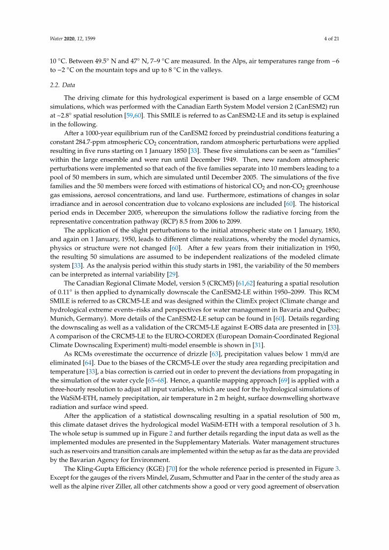
Water 2020, 12, 1599 4 of 21

10 ◦C. Between 49.5◦ N and 47◦ N, 7–9 ◦C are measured. In the Alps, air temperatures range from −6to −2 ◦C on the mountain tops and up to 8 ◦C in the valleys.

2.2. Data

The driving climate for this hydrological experiment is based on a large ensemble of GCMsimulations, which was performed with the Canadian Earth System Model version 2 (CanESM2) runat ~2.8◦ spatial resolution [59,60]. This SMILE is referred to as CanESM2-LE and its setup is explainedin the following.

After a 1000-year equilibrium run of the CanESM2 forced by preindustrial conditions featuring aconstant 284.7-ppm atmospheric CO2 concentration, random atmospheric perturbations were appliedresulting in five runs starting on 1 January 1850 [33]. These five simulations can be seen as “families”within the large ensemble and were run until December 1949. Then, new random atmosphericperturbations were implemented so that each of the five families separate into 10 members leading to apool of 50 members in sum, which are simulated until December 2005. The simulations of the fivefamilies and the 50 members were forced with estimations of historical CO2 and non-CO2 greenhousegas emissions, aerosol concentrations, and land use. Furthermore, estimations of changes in solarirradiance and in aerosol concentration due to volcano explosions are included [60]. The historicalperiod ends in December 2005, whereupon the simulations follow the radiative forcing from therepresentative concentration pathway (RCP) 8.5 from 2006 to 2099.

The application of the slight perturbations to the initial atmospheric state on 1 January, 1850,and again on 1 January, 1950, leads to different climate realizations, whereby the model dynamics,physics or structure were not changed [60]. After a few years from their initialization in 1950,the resulting 50 simulations are assumed to be independent realizations of the modeled climatesystem [33]. As the analysis period within this study starts in 1981, the variability of the 50 memberscan be interpreted as internal variability [29].

The Canadian Regional Climate Model, version 5 (CRCM5) [61,62] featuring a spatial resolutionof 0.11◦ is then applied to dynamically downscale the CanESM2-LE within 1950–2099. This RCMSMILE is referred to as CRCM5-LE and was designed within the ClimEx project (Climate change andhydrological extreme events–risks and perspectives for water management in Bavaria and Québec;Munich, Germany). More details of the CanESM2-LE setup can be found in [60]. Details regardingthe downscaling as well as a validation of the CRCM5-LE against E-OBS data are presented in [33].A comparison of the CRCM5-LE to the EURO-CORDEX (European Domain-Coordinated RegionalClimate Downscaling Experiment) multi-model ensemble is shown in [31].

As RCMs overestimate the occurrence of drizzle [63], precipitation values below 1 mm/d areeliminated [64]. Due to the biases of the CRCM5-LE over the study area regarding precipitation andtemperature [33], a bias correction is carried out in order to prevent the deviations from propagating inthe simulation of the water cycle [65–68]. Hence, a quantile mapping approach [69] is applied with athree-hourly resolution to adjust all input variables, which are used for the hydrological simulations ofthe WaSiM-ETH, namely precipitation, air temperature in 2 m height, surface downwelling shortwaveradiation and surface wind speed.

After the application of a statistical downscaling resulting in a spatial resolution of 500 m,this climate dataset drives the hydrological model WaSiM-ETH with a temporal resolution of 3 h.The whole setup is summed up in Figure 2 and further details regarding the input data as well as theimplemented modules are presented in the Supplementary Materials. Water management structuressuch as reservoirs and transition canals are implemented within the setup as far as the data are providedby the Bavarian Agency for Environment.

The Kling-Gupta Efficiency (KGE) [70] for the whole reference period is presented in Figure 3.Except for the gauges of the rivers Mindel, Zusam, Schmutter and Paar in the center of the study area aswell as the alpine river Ziller, all other catchments show a good or very good agreement of observation

Water 2020, 12, 1599 5 of 21

and simulation (KGE > 0.5). Due to the undercatch of mountainous precipitation gauges [41,71,72],most alpine and pre-alpine catchments show a KGE between 0.5 and 0.7.

Figure 2. Schematic representation of the hydrometeorological model and processing chain.

Figure 3. KGE for all 98 catchments in hydrological Bavaria during the reference period (1981–2010).

Water 2020, 12, 1599 6 of 21

3. Methods

The hydrological regime characterized by the Pardé coefficient is governed by the climate(temperature and precipitation), topography (elevation and exposition) and further features (land use,soils, geology) of the catchment [2]. To evaluate the WaSiM-ETH setup for this experiment, the Pardécoefficients are calculated for the reference period using observed runoffs and WaSiM-ETH simulationsdriven by observational meteorological data. After that, monthly Pardé coefficients are calculated usingthe climate model data for all 98 catchments and 50 members during the reference period resultingin 4900 regimes. An agglomerative hierarchical clustering using the complete linkage algorithmwith Euclidean distance is applied on these 4900 regimes [56,73–75]. The number of clusters for thisalgorithm is chosen by the user. As this choice is arbitrary, there are several strategies to evaluate thenumber of clusters. On one hand, external criteria such as class labels (“nival”, “nivopluvial”, “pluvial”)can be applied to compare the results of the cluster analysis to these labels, which are known to the userbeforehand [76]. On the other hand, relative criteria can be found, which evaluate different clusteringschemes, resulting by the same algorithm but with a varying number of clusters [77]. Charrad et al. [77]provide a toolbox containing a set of different indices to evaluate clustering schemes. For this study,we apply 27 indices, constraining them to a cluster number between 4 and 10 (see SupplementaryMaterials for further details). Following the rule of majority [77], the highest number of indices, namely10, propose six clusters. Therefore, we apply the hierarchical clustering algorithm with six clusters toall 4900 runoff regimes.

If more than 10 regimes of the 50 total regimes per catchment are classified within a cluster,the catchment is categorized into the respective class. This also allows a regime to belong to two ormore classes. The large ensemble of 50 members thereby contributes to the robustness of this clusteranalysis, as the application of this method using single members of the WaSiM-LE leads to differingresults. Furthermore, this methodology allows the internal variability of the climatic drivers to bereflected in the classification of runoff regimes.

4. Results

The spatial distribution of the cluster analysis for the reference period is presented in Figure 4.The validation of the hydrological model setup applying observational meteorological data for eachclustering region is shown in Figure 5. Thereby, a root-mean-square error (RMSE) of 0.09 on averagefor all months and catchments shows sufficient agreement of the model and observations. For mainlyrainfall-driven catchments (Region 4, 5 and 6), the comparison of simulated and observed Pardécoefficients show very good agreement. In the snowmelt-influenced catchments, the height andposition of the peak is not fully reproduced. Partially, this can be explained with the observationalmeteorological data underestimating solid precipitation. The undercatch of snow can amount up to40% for shielded gauges and 80% for unshielded gauges [71,78–80]. Grossi et al. [81] find deviationsof −15% to −66% in the northern Italian Alps. Additionally, the station density in the Alps is nothigh enough [82]. As these observations influence the snowfall in the WaSiM-LE as part of the biascorrection, the snowmelt-induced runoff is underestimated as well. Apart from these deviations,the general characteristics of each regime class are preserved.

Region 1 shows a (glacio-)nival regime with its peak in June and July (see Figure 6). The threealpine gauges of the Inn and the Oetztaler Ache belong to this regime class, whereby the OetztalerAche has its peak flow in July, which is why it is classified as glacio-nival regime [37]. Region 2 alsohas its peak flow in June, but it is simulated earlier during May due to the underestimation of snowfalland snowmelt. The regime is more balanced than the (glacio-)nival regime with a less spiky peak andhigher flows during the winter. Therefore, it is classed as a nival transition regime. The respectivecatchments are located in the Pre-Alps and Alpine Foreland. Region 3 can be categorized as nivo-pluvialregime. The peak in April is caused by a combination of rainfall and snowmelt processes, whereasthe coefficients > 1 during June to September are governed by the rain regime only. Region 4 showsa very balanced flow regime. The catchments are located in the center of the study area near the

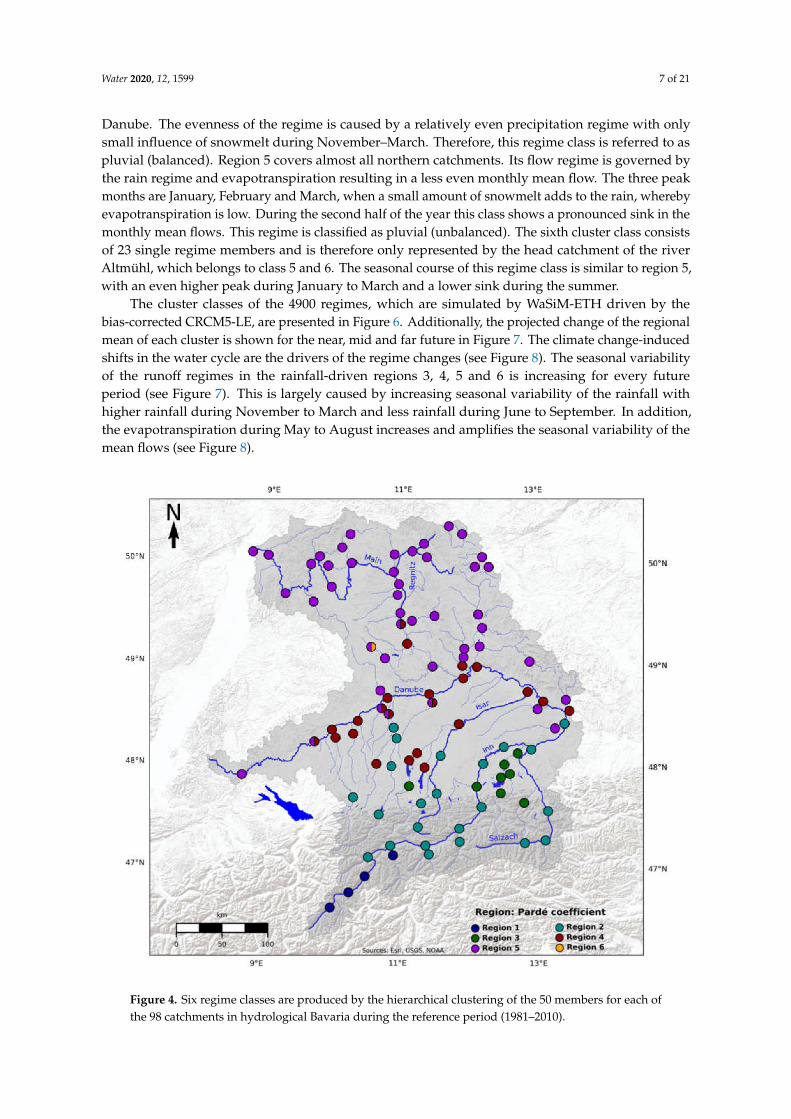
Water 2020, 12, 1599 7 of 21

Danube. The evenness of the regime is caused by a relatively even precipitation regime with onlysmall influence of snowmelt during November–March. Therefore, this regime class is referred to aspluvial (balanced). Region 5 covers almost all northern catchments. Its flow regime is governed bythe rain regime and evapotranspiration resulting in a less even monthly mean flow. The three peakmonths are January, February and March, when a small amount of snowmelt adds to the rain, wherebyevapotranspiration is low. During the second half of the year this class shows a pronounced sink in themonthly mean flows. This regime is classified as pluvial (unbalanced). The sixth cluster class consistsof 23 single regime members and is therefore only represented by the head catchment of the riverAltmühl, which belongs to class 5 and 6. The seasonal course of this regime class is similar to region 5,with an even higher peak during January to March and a lower sink during the summer.

The cluster classes of the 4900 regimes, which are simulated by WaSiM-ETH driven by thebias-corrected CRCM5-LE, are presented in Figure 6. Additionally, the projected change of the regionalmean of each cluster is shown for the near, mid and far future in Figure 7. The climate change-inducedshifts in the water cycle are the drivers of the regime changes (see Figure 8). The seasonal variabilityof the runoff regimes in the rainfall-driven regions 3, 4, 5 and 6 is increasing for every futureperiod (see Figure 7). This is largely caused by increasing seasonal variability of the rainfall withhigher rainfall during November to March and less rainfall during June to September. In addition,the evapotranspiration during May to August increases and amplifies the seasonal variability of themean flows (see Figure 8).

Figure 4. Six regime classes are produced by the hierarchical clustering of the 50 members for each ofthe 98 catchments in hydrological Bavaria during the reference period (1981–2010).

Water 2020, 12, 1599 8 of 21

Figure 5. Pardé coefficients for the reference period 1981–2010. The coefficients calculated withmeasurements are marked as solid line, whereas the dashed lines represent WaSiM-ETH simulationsdriven by observational meteorological data. The colored lines show the mean for each region and thegray lines show every single catchment.

Figure 6. Pardé coefficients for the reference period 1981–2010 are calculated on the basis of all 50members of the WaSiM-LE (gray lines). The colored lines show the regional mean for each cluster.

Water 2020, 12, 1599 9 of 21

Figure 7. The regional mean Pardé coefficients during the reference period, near, mid and far future.Shaded areas represent the range of all catchments within each cluster class.

Figure 8. Components of the water cycle simulated by the WaSiM-LE for the reference period, near,mid and far future (same color signatures as in Figure 7). The lines represent the regional mean overthe catchments of each cluster class (weighted by the area of the catchment) and the shaded areas showthe range of all catchments within the cluster.

Water 2020, 12, 1599 10 of 21

The catchments with mainly snowmelt-driven (glacio-)nival and nival transition regimes arelocated in the Alps, pre-alpine regions and the Alpine Foreland, whereby the sources of these rivers arein the Alps and Pre-Alps. Climate change-induced higher temperatures and earlier snowmelt causethe monthly peak to occur less pronounced and earlier in the season during the mid and far future,respectively. The relative importance of snowmelt for the monthly discharge decreases, whereas liquidprecipitation will increasingly contribute to the runoff during winter and early spring. Generally,catchments of these both regime types will show a more balanced seasonal runoff in the future.

The monthly peak of the nivo-pluvial catchments shifts from April to March in the far future,whereby this peak gets more intense. The normalized monthly discharge from December to Marchincreases in every future period, while from July to October a severe decline is found. The contributionof snowmelt decreases by every future period, leading to a higher relative importance of rainfall.

The normalized monthly runoff of all three pluvial regime types increases in the first half ofthe year by every future period and decreases in the second half of the season. These shifts can beaddressed to changes in the rainfall regime and rising evapotranspiration during May to August.These results are consistent with several regional studies, which analyze climate change impacts onhydrological characteristics on catchments in the Alps and Alpine Foreland [7,11,34,35,37,38,83,84].

In order to assess this impact on the categorization of the runoff regimes, the Euclidean distancesof the 4900 Pardé coefficients of the reference period to the 3 × 4900 coefficients of the near, mid and farfuture are calculated. According to these distances, the regimes of the future are categorized into thecluster classes of the reference period. The result of this classification shows if the changing climate iscausing a shift of the regime class until 2011–2040, 2041–2070 or 2071–2099 (see Figures 9–11). Table 1summarizes the number of catchments within each cluster class.

Compared to the reference period, eight catchments will change their regime classes in the nearfuture. These are nival and nivo-pluvial catchments in the Alpine Foreland, where the influenceof snow decreases, which causes a shift towards a pluvial class. However, these catchments arecategorized belonging to both regime classes. This means that the change in their regimes is within therange of natural variability for the near future.

During the mid-future, a shift in the regime class is examined for 23 catchments, which equalsto 23% of all 98 catchments (see Figure 10). The number of catchments within the snowmelt-relatedclasses ((glacio-)nival, nival transition, nivo-pluvial) decreases from 35 to 30. These shifting catchmentsare located in the Alpine Foreland, where the importance of snowmelt declines. In this region, thepluvial categories gain new members. In the center and north of the study area, both pluvial classesstill dominate, whereby some catchments of the Danube and near the Danube change their categoryfrom balanced to both balanced and unbalanced.

For the far future, an even more severe shift of regime classes is found (see Figure 11). Almost allcatchments in the Alpine Foreland except for two Inn gauges turn into pluvial or nivo-pluvial regimes.From the (glacio-)nival class, only the Oetztaler Ache remains. The former nivo-pluvial regimesaround Lake Chiemsee change to pluvial regimes. The number of catchments within the (glacio-)nival,nival transition and nivo-pluvial classes further decreases to 22. The unbalanced pluvial regime class(Region 5) becomes the dominant regime class with 61% of all catchments.

In sum, 42 of 98 catchments shift their regime class compared to the reference period, which amountsto 43%. From the mid to far future, the most severe change is found. In comparison to 2041–2070,30 catchments change their respective regime class, which equals 31%.

Water 2020, 12, 1599 11 of 21

Figure 9. Hierarchical clustering of the mean regime of the 50 members of each catchment during thenear future (2011–2040) into the cluster classes of the reference period.

Figure 10. Hierarchical clustering of the mean regime of the 50 members of each catchment during themid-future (2041–2070) into the cluster classes of the reference period.

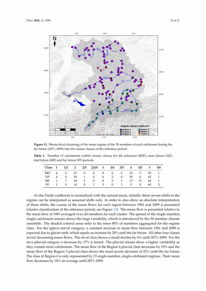
Water 2020, 12, 1599 12 of 21

Figure 11. Hierarchical clustering of the mean regime of the 50 members of each catchment during thefar future (2071–2099) into the cluster classes of the reference period.

Table 1. Number of catchments within cluster classes for the reference (REF), near future (NF),mid future (MF) and far future (FF) periods.

Class 1 1/2 2 2/3 2/3/4 3 3/4 3/5 4 4/5 5 5/6

REF 4 0 23 0 0 8 0 0 18 5 39 1NF 4 0 18 1 0 6 2 0 18 6 42 1MF 1 1 18 0 0 8 0 1 13 11 44 1FF 1 0 14 0 1 5 0 1 5 8 60 3

As the Pardé coefficient is normalized with the annual mean, initially, these severe shifts in theregime can be interpreted as seasonal shifts only. In order to also allow an absolute interpretationof these shifts, the course of the mean flows for each region between 1981 and 2099 is presented(cluster classification of the reference period; see Figure 12). The mean flow is presented relative tothe mean flow of 1981 averaged over all members for each cluster. The spread of the single-member,single-catchment courses shows the large variability, which is introduced by the 50-member climateensemble. The shaded colored areas refer to the inner 80% of members aggregated for the regimeclass. For the (glacio-)nival category, a constant increase in mean flow between 1981 and 2099 isexpected due to glacier melt, which equals an increase by 20% until the far future. All other four classesreveal decreasing mean flows. The nival class shows a small decline by 6% until 2071–2099. For thenivo-pluvial category a decrease by 17% is found. The pluvial classes show a higher variability asthey contain more catchments. The mean flow of the Region 4 pluvial class decreases by 19% and themean flow of the Region 5 pluvial class shows the most severe decrease of 22% until the far future.The class of Region 6 is only represented by 23 single-member, single-catchment regimes. Their meanflow decreases by 18% on average until 2071–2099.

Water 2020, 12, 1599 13 of 21

Figure 12. Annual MQ for each region relative to the average MQ of 1981 (mean over all catchments ofthe cluster). Gray lines denote every member of each catchment. The colored line shows the mean ofall members and catchments per region. The colored shaded area corresponds to the range between the10th and 90th percentile of each cluster.

The variability of annual mean flows introduced by the spread of the 50-member large ensemblecan also be expressed with the coefficient of variation (CV). The CV is defined as the standard deviationnormalized by the mean. In Table 2, we present the CV of the mean 30-year MQ for the reference andthe three future periods, whereby the CV of all contributing catchments is averaged for the respectiveregion. The values illustrate that the variability of individual extreme years (Figure 12) is filtered outby averaging the mean flows over 30 years. Nevertheless, coefficients of variation between 2% and 8%are shown, with a steady increase in variability projected for the future periods.

Table 2. Coefficient of variation of the mean 30-year MQ within cluster classes for the reference (REF),near future (NF), mid future (MF) and far future (FF) periods.

Region 1 Region 2 Region 3 Region 4 Region 5 Region 6

REF 4.90% 2.01% 2.73% 3.60% 5.13% 6.05%NF 6.40% 2.80% 3.71% 4.70% 6.68% 7.12%MF 6.84% 3.00% 4.27% 5.82% 7.26% 6.87%FF 7.40% 3.01% 4.61% 6.35% 7.78% 7.39%

5. Discussion

5.1. Advantages of the Clustering Approach

The application of hierarchical clustering on a large ensemble of Pardé coefficients enables a robustclassification. The driving climate just differs by internal variability, and due to that also the simulatedrunoff regimes vary. As the driving climate has a big impact on the runoff regime, the most extrememembers at the edges of the ensemble in terms of rainfall, snowfall and air temperature would lead toa different categorization for some catchments. Hence, the broad database of 1500 years simulatedrunoff per 30-year period ensures that individual extreme members do not distort the classification.Furthermore, this approach allows catchments to be assigned to more than one regime category.This shows the variability of the flow regime according to its driving climate. As hydrological systems

Water 2020, 12, 1599 14 of 21

behave non-linearly, the internal variability of the climate system leads to an internal variability withinthe flow regimes. This can be represented by shared categories.

Pardé [12], Grimm ([85] for Europe) or subsequent studies (Mader et al. [86] for Austria) suggesteda categorization of regimes for different regions based on the timing and order of the monthly maximumand minimum coefficients. Since runoff regimes represent a dynamical system [87], these kinds ofrigid categorization would lead to non-representative classification results, especially for catchments,where the peak of mean flows is not pronounced [56].

In contrast, the agglomerative hierarchical clustering featuring the complete linkage algorithmuses the Euclidean distance to cluster the regimes, which includes the whole course of the regime,not only the position of the peaks. In our case, region 4 shows a mixed regime without pronouncedpeaks and sinks, as it is driven by southern tributaries with nival or nivo-pluvial regimes as well asby the rainfall regime, which directly affects the catchment. The clustering algorithm includes theseasonal runoff information of all 12 months leading to a robust classification, which is also representedby the spatial distribution of region 4 in Figure 4. Furthermore, the pluvial regimes of regions 5 and 6show a similar timing of the peak and sink. The classical categorizations of Pardé [12], Grimm [85] orMader et al. [86] would have included both classes in one category. Though, the Euclidean distance ofregions 5 and 6 causes the hierarchical clustering algorithm to divide both classes. As region 6 shows avery pronounced sink during July to October (Figure 6) and the mean flow in this region decreases(Figure 12), it is important that the categorization reflects this behavior.

Moreover, the choice of the number of clusters is objectively determined by the use of the set ofindices by Charrad et al. [77]. Hence, the whole procedure of selecting the number of clusters, creatingthe classes and analyzing the regime changes due to climate change are only driven by the data andare therefore objective and generally applicable in any region of the world.

Therefore, this classification method is on the one hand more flexible than methods focusing onthe peaks only and on the other hand this method is nonarbitrary [56].

5.2. Socio-Economic Impacts of the Runoff Regime Change in Bavaria

The changes in the runoff regime impact several socio-economic sectors as well as the ecologyof the river and its surrounding areas [16]. In order to assess the ecological impact, river basinswould have to be considered individually and other factors such as changes in water temperature,chemical composition, flood frequency and low water frequency would have to be additionally takeninto account.

Therefore, we discuss possible socio-economic impacts in the following. Generally, changes in thehydrological regime have the potential to increase competition over water, as the availability of waterchanges in terms of time and quantity [3]. Therefore, sustainable water resource management has toadapt not only to the physical changes, which are projected within this study, but also to socio-economicshifts in land and water use.

One of these possible changes relates to the water use for irrigation. In Bavaria, which coversbig parts of the study area, there are 93,300 forestry companies and agricultural enterprises growingcereals, vegetables, grapes and hops, producing fodder for livestock and keeping dairy cattle andlivestock (status: 2013 [88]). During the past decades, only 1% of all agricultural land in Bavaria wasirrigated regularly and officially [89,90]. The need for irrigation was mainly dependent on the crop,with predominantly various vegetables and potatoes being irrigated. Due to rising evapotranspirationand less rainfall during the summer (see Figure 7), the water demand for irrigation is expected toincrease drastically [91,92]. In the study area, especially the cultivation of maize and vegetables, such aspotatoes, cabbage, carrots and onions will be affected by the decline in summer precipitation leadingto increasing irrigation demands. In the catchments north of the Danube, the dry and hot summerof 2018 has already induced many farmers to irrigate their fields. Irrigation water is drawn fromgroundwater or from riverbanks by wells, or it is directly pumped from reservoirs, lakes and rivers [88].

Water 2020, 12, 1599 15 of 21

Since groundwater levels are expected to fall [93] and the mean flows during summer decrease in thepluvial regime classes (Figure 7), there is an increasing risk of irrigation water scarcity.

Hydropower contributes 14.4%, equaling 12.2 TWh, to the power generation in Bavaria (status:2017, [94]). Most of the hydropower plants are located at the southern tributaries to the Danube,the Danube itself and the river Main [95]. The seasonality of the runoff regime has a big impacton run-of-river power plants as they are dependent on the actual runoff, whereas reservoir powerplants can bridge low-flow periods by damming up water. The hydropower plants at the Main aswell as around 70% of the power plants of the Danube tributaries are run-of-river power plants [20].As the amount of generated power can be expressed as approximately linearly dependent on therunoff volume [20], we can include the changes in seasonality (Figure 7) and the course of mean flows(Figure 12) to estimate the impact on seasonal hydropower power generation. For the hydropowerplants in the pluvial regions, the potential for power generation sinks severely during the second halfof the year due to lower mean flow periods. However, the hydropower plants, which are located closerto the Alps in the nival regions, show a more balanced power generation potential in the future asincreasing rainfall and decreasing snow storage during the winter ensure an even flow seasonality.Though, the annual power generation is projected to decrease according to the mean flows (Figure 12).These findings tie in with the results of the study of Koch et al. [20], which focuses on the hydropowerin the Upper Danube basin.

Fossil fuel-based power plants, such as coal-, gas-, waste- and oil-fired as well as nuclear plantsalso demand water in order to cool down the steam in the condenser. The biggest power plants inthe study area are located at the larger rivers, the Danube, Isar and Main. Their water demand isdependent on the power plant utilization, but also on the meteorological conditions [21], wherebyat a constant utilization more cooling water is needed during the summer. The decline of annualmean flows and seasonal mean flows during the second half of the year in pluvial regimes shouldbe considered when power plants are managed. However, due to the nuclear and coal phaseout inGermany until 2022 and 2038 [96,97], the effect on power plant cooling due to regime changes areunlikely to have big impact by the mid or far future.

The inland waterway transport in the study area is mainly focused on the federal waterways Mainand Danube and their interconnection, the Main-Danube canal, with a cargo handling of 6–15 Mt/aduring the last 30 years [98]. Conditions of lower flow reduce the possible maximum draught of vessels,which thereby decrease the efficiency of inland water transport [24]. Furthermore, the risk of groundingand collisions rises due to reduced depth and width of the fairway. The analysis of the mean flowsdoes not include any extreme low-flow conditions, but the trend of decreasing mean flows betweenAugust and October at the rivers Danube and Main may cause limitations for the shipping. For allgauges along the German federal waterways, the mean flow of August to October decreases by 21%,25% and 44% on average until the near, mid and far future, respectively. Further analysis of extremelow-flow events is necessary to assess the frequency and duration of periods, where navigability is notonly reduced, but severely affected or even completely restricted.

6. Conclusions

The WaSiM-LE, a large ensemble of hydrological simulations, which is driven by the regionalclimate simulations of the CRCM5-LE, is used to categorize runoff regimes in hydrological Bavaria.The application of a large ensemble for this analysis provides added value as the 50 members covera range of climatic internal variability representing the dynamical characteristics of runoff regimes.This leads to a broad database of regimes per catchment and time period, which enables a robustclustering analysis. In the study area, six regime classes are found for the reference period: (glacio-)nival,nival (transition), nivo-pluvial, pluvial (balanced), pluvial (unbalanced) and a second, more unbalancedpluvial class.

The CRCM5-LE featuring the high-emission scenario RCP 8.5 shows major changes in the drivingclimate for all future periods. The findings of earlier snowmelt, less snowfall, more evapotranspiration

Water 2020, 12, 1599 16 of 21

and a changing rainfall regime towards the future tie in with the results of other local and regionalstudies. Due to these severe impacts of climate change on the water cycle, a shift of the regimeclass is found for 8%, 23% and 43% of the catchments until the near, mid and far future, respectively.Until 2070–2099, no kind of nival regime will persist in the Alpine Foreland except for two gauges ofthe river Inn. The sinks during summer of all regimes north of the Alps become more pronounced foreach future period resulting in a big increase of the unbalanced pluvial region 5. This class shows avery distinct seasonal behavior with Pardé coefficients around 0.2 during August to October in thefar future.

The change of the seasonal mean flows will be a major challenge for water management and willhave a big impact on stakeholders in the respective catchments. We discussed impacts on the watersupply for irrigation, the industrial water demand, and the navigability of waterways. Especially forrun-of-river hydropower plants located in catchments in a pluvial regime class, the more pronouncedseasonality with decreasing mean flows in the second half of the year will lead to severe losses in thepotential of power generation.

Supplementary Materials: The following refer to [99–104] and are available online at http://www.mdpi.com/2073-4441/12/6/1599/s1, Figure S1: Median of the seasonal temperatures for the uncorrected (BC0) and biascorrected (BC1) climate model ensemble as well as their difference (BC0–BC1), Figure S2: Median of the seasonalprecipitation for the uncorrected (BC0) and bias corrected (BC1) climate model ensemble as well as their difference(BC0–BC1), Table S1: Data used for the WaSiM-ETH setup, Table S2: Modules applied in the WaSiM-ETH setup,Table S3: Optimal number of clusters for 4900 Pardé coefficients chosen by 27 different indices. The indices havebeen restricted to the range of four to ten cluster classes.

Author Contributions: Conceptualization, B.P.; WaSiM-ETH setup, F.W.; methodology of clustering analysis, B.P.;software, B.P. and F.W.; validation, F.W.; formal analysis, B.P.; investigation, B.P.; resources, R.L.; data curation,B.P., F.W.; writing—original draft preparation, B.P.; writing—review and editing, B.P., F.W. and R.L.; visualization,B.P. and F.W.; supervision, R.L.; project administration, R.L.; funding acquisition, R.L. All authors have read andagreed to the published version of the manuscript.

Funding: This research was funded by the Bavarian State Ministry for the Environment and ConsumerProtection. Computations with the CRCM5 and WaSiM-ETH for the ClimEx project were made on the SuperMUCsupercomputer at Leibniz Supercomputing Centre (LRZ) of the Bavarian Academy of Sciences and Humanities.The operation of this supercomputer is funded via the Gauss Centre for Supercomputing (GCS) by the GermanFederal Ministry of Education and Research and the Bavarian State Ministry of Education, Science and the Arts.

Acknowledgments: We thank all members of the ClimEx project working group for their contributions to produceand analyze the CanESM2-LE, CRCM5-LE and WaSiM-LE. Especially, we want to thank Raul Wood for thecreation of the meteorological reference data, which was used for the bias adjustment and Magdalena Mittermeierfor the analysis of the differences between BC0 and BC1. The CRCM5 was developed by the ESCER centre ofUniversité du Québec a Montréal (UQAM; http://www.escer.uqam.ca) in collaboration with Environment andClimate Change Canada. We acknowledge Environment and Climate Change Canada’s Canadian Centre forClimate Modelling and Analysis for executing and making available the CanESM2 Large Ensemble simulationsused in this study, and the Canadian Sea Ice and Snow Evolution Network for proposing the simulations. We alsothank the developer of WaSiM-ETH (http://www.wasim.ch/de/), Jörg Schulla for his support.

Conflicts of Interest: The authors declare no conflict of interest. The funders had no role in the design of thestudy; in the collection, analyses, or interpretation of data; in the writing of the manuscript, or in the decision topublish the results.

References

1. Messerli, B.; Viviroli, D.; Weingartner, R. Mountains of the World: Vulnerable Water Towers for the 21stCentury. In Special Report Number 13. The Royal Colloquium: Mountain Areas: A Global Resource; Springer:Berlin/Heidelberg, Germany, 2004; pp. 29–34. [CrossRef]

2. Bormann, H. Runoff regime changes in German rivers due to climate change. Erdkunde 2010, 64, 257–279.[CrossRef]

3. Strasser, U.; Marke, T.; Braun, L.; Escher-Vetter, H.; Juen, I.; Kuhn, M.; Maussion, F.; Mayer, C.; Nicholson, L.;Niedertscheider, K.; et al. The Rofental: A high Alpine research basin (1890 m–3770 m a.s.l.) in the ÖtztalAlps (Austria) with over 150 years of hydro-meteorological and glaciological observations. Earth Syst. Sci.Data 2018, 10, 151–171. [CrossRef]

Water 2020, 12, 1599 17 of 21

4. Ionita, M.; Badaluta, C.-A.; Scholz, P.; Chelcea, S. Vanishing river ice cover in the lower part of the Danubebasin—Signs of a changing climate. Sci. Rep. 2018, 8, 7948. [CrossRef] [PubMed]

5. Beniston, M. Impacts of climatic change on water and associated economic activities in the Swiss Alps.J. Hydrol. 2012, 412–413, 291–296. [CrossRef]

6. Gobiet, A.; Kotlarski, S.; Beniston, M.; Heinrich, G.; Rajczak, J.; Stoffel, M. 21st century climate change in theEuropean Alps—A review. Sci. Total Environ. 2014, 493, 1138–1151. [CrossRef]

7. Milano, M.; Reynard, E.; Bosshard, N.; Weingartner, R. Simulating future trends in hydrological regimes inWestern Switzerland. J. Hydrol. Reg. Stud. 2015, 4, 748–761. [CrossRef]

8. Stagl, J.; Hattermann, F. Impacts of Climate Change on the Hydrological Regime of the Danube River and ItsTributaries Using an Ensemble of Climate Scenarios. Water 2015, 7, 6139–6172. [CrossRef]

9. Rojas, R.; Feyen, L.; Bianchi, A.; Dosio, A. Assessment of future flood hazard in Europe using a large ensembleof bias-corrected regional climate simulations. J. Geophys. Res. 2012, 117, D17109. [CrossRef]

10. Schneider, C.; Laizé, C.L.R.; Acreman, M.C.; Flörke, M. How will climate change modify river flow regimesin Europe? Hydrol. Earth Syst. Sci. 2013, 17, 325–339. [CrossRef]

11. Köplin, N.; Viviroli, D.; Schädler, B.; Weingartner, R. How does climate change affect mesoscale catchmentsin Switzerland?—A framework for a comprehensive assessment. Adv. Geosci. 2010, 27, 111–119. [CrossRef]

12. Pardé, M. Fleuves et Rivières; Armand Colin: Paris, France, 1933; p. 224.13. Gaudry, M.M.C.; Gutknecht, D.; Parajka, J.; Perdigão, R.A.P.; Blöschl, G. Seasonality of runoff and precipitation

regimes along transects in Peru and Austria. J. Hydr. Hydromech. 2017, 65, 347–358. [CrossRef]14. Cañedo-Argüelles, M.; Kefford, B.J.; Piscart, C.; Prat, N.; Schäfer, R.B.; Schulz, C.-J. Salinisation of rivers:

An urgent ecological issue. Environ. Pollut. 2013, 173, 157–167. [CrossRef] [PubMed]15. Poff, N.L.; Allan, J.D.; Bain, M.B.; Karr, J.R.; Prestegaard, K.L.; Richter, B.D.; Sparks, R.E.; Stromberg, J.C.

The Natural Flow Regime. A paradigm for river conservation and restoration. BioScience 1997, 47, 769–784.[CrossRef]

16. Poff, N.L.; Zimmerman, J.K.H. Ecological responses to altered flow regimes: A literature review to informthe science and management of environmental flows. Freshw. Biol. 2010, 55, 194–205. [CrossRef]

17. Bruckerhoff, L.A.; Leasure, D.R.; Magoulick, D.D. Flow–ecology relationships are spatially structured anddiffer among flow regimes. J. Appl. Ecol. 2019, 56, 398–412. [CrossRef]

18. Schleuter, M. Computing the degradation of riparian floodplains by means of a water-level difference curve.Hydrol. Wasserbewirtsch. 2010, 54, 360–367.

19. Gaudard, L.; Romerio, F. The future of hydropower in Europe: Interconnecting climate, markets and policies.Environ. Sci. Policy 2014, 37, 172–181. [CrossRef]

20. Koch, F.; Prasch, M.; Bach, H.; Mauser, W.; Appel, F.; Weber, M. How Will Hydroelectric Power GenerationDevelop under Climate Change Scenarios? A Case Study in the Upper Danube Basin. Energies 2011, 4,1508–1541. [CrossRef]

21. Koch, H.; Vögele, S. Dynamic modelling of water demand, water availability and adaptation strategies forpower plants to global change. Ecol. Econ. 2009, 68, 2031–2039. [CrossRef]

22. Bär, R.; Rouholahnejad, E.; Rahman, K.; Abbaspour, K.C.; Lehmann, A. Climate change and agriculturalwater resources: A vulnerability assessment of the Black Sea catchment. Environ. Sci. Policy 2015, 46, 57–69.[CrossRef]

23. Jonkeren, O.; Rietveld, P.; van Ommeren, J.; te Linde, A. Climate change and economic consequences forinland waterway transport in Europe. Reg. Environ. Chang. 2014, 14, 953–965. [CrossRef]

24. Nilson, E.; Krahe, P. Navigation on the rhine river and climate change. Geogr. Rundsch. 2013, 65, 26–33.25. Stoelzle, M.; Blauhut, V.; Kohn, I.; Weiler, M.; Stahl, K. Niedrigwasser in Süddeutschland Analysen, Szenarien und

Handlungsempfehlungen; Arbeitskreis KLIWA, Ed.; Bayerisches Landesamt für Umwelt: Hof, Germany, 2018;p. 95.

26. Ehsani, N.; Vörösmarty, C.J.; Fekete, B.M.; Stakhiv, E.Z. Reservoir operations under climate change: Storagecapacity options to mitigate risk. J. Hydrol. 2017, 555, 435–446. [CrossRef]

27. Fatichi, S.; Rimkus, S.; Burlando, P.; Bordoy, R.; Molnar, P. High-resolution distributed analysis of climate andanthropogenic changes on the hydrology of an Alpine catchment. J. Hydrol. 2015, 525, 362–382. [CrossRef]

28. Willkofer, F.; Schmid, F.-J.; Komischke, H.; Korck, J.; Braun, M.; Ludwig, R. The impact of bias correctingregional climate model results on hydrological indicators for Bavarian catchments. J. Hydrol. Reg. Stud. 2018,19, 25–41. [CrossRef]

Water 2020, 12, 1599 18 of 21

29. Deser, C.; Phillips, A.; Bourdette, V.; Teng, H. Uncertainty in climate change projections: The role of internalvariability. Clim. Dyn. 2012, 38, 527–546. [CrossRef]

30. Hawkins, E.; Sutton, R. The potential to narrow uncertainty in regional climate predictions. Bull. Am.Meteorol. Soc. 2009, 90, 1095–1108. [CrossRef]

31. Von Trentini, F.; Leduc, M.; Ludwig, R. Assessing natural variability in RCM signals: Comparison of a multimodel EURO-CORDEX ensemble with a 50-member single model large ensemble. Clim. Dyn. 2019, 53,1963–1979. [CrossRef]

32. Martel, J.-L.; Mailhot, A.; Brissette, F.; Caya, D. Role of Natural Climate Variability in the Detection ofAnthropogenic Climate Change Signal for Mean and Extreme Precipitation at Local and Regional Scales.J. Clim. 2018, 31, 4241–4263. [CrossRef]

33. Leduc, M.; Mailhot, A.; Frigon, A.; Martel, J.-L.; Ludwig, R.; Brietzke, G.; Giguère, M.; Brissette, F.; Turcotte, R.;Braun, M.; et al. The ClimEx Project: A 50-Member Ensemble of Climate Change Projections at 12-kmResolution over Europe and Northeastern North America with the Canadian Regional Climate Model(CRCM5). J. Appl. Meteorol. Clim. 2019, 58, 663–693. [CrossRef]

34. Coppola, E.; Raffaele, F.; Giorgi, F. Impact of climate change on snow melt driven runoff timing over theAlpine region. Clim. Dyn. 2018, 51, 1259–1273. [CrossRef]

35. Farinotti, D.; Usselmann, S.; Huss, M.; Bauder, A.; Funk, M. Runoff evolution in the Swiss Alps: Projectionsfor selected high-alpine catchments based on ENSEMBLES scenarios. Hydrol. Process. 2012, 26, 1909–1924.[CrossRef]

36. Döll, P.; Schmied, H.M. How is the Impact of Climate Change on River Flow Regimes Related to the Impact on MeanAnnual Runoff? A Global-Scale Analysis; IOP Publishing Ltd: Bristol, UK, 2012; Volume 7. [CrossRef]

37. Hanzer, F.; Förster, K.; Nemec, J.; Strasser, U. Projected cryospheric and hydrological impacts of 21st centuryclimate change in the Ötztal Alps (Austria) simulated using a physically based approach. Hydrol. Earth Syst.Sci. 2018, 22, 1593–1614. [CrossRef]

38. Addor, N.; Rössler, O.; Köplin, N.; Huss, M.; Weingartner, R.; Seibert, J. Robust changes and sources ofuncertainty in the projected hydrological regimes of Swiss catchments. Water Resour. Res. 2014, 50, 7541–7562.[CrossRef]

39. Ludwig, R.; May, I.; Turcotte, R.; Vescovi, L.; Braun, M.; Cyr, J.-F.; Fortin, L.-G.; Chaumont, D.; Biner, S.;Chartier, I.; et al. The role of hydrological model complexity and uncertainty in climate change impactassessment. Adv. Geosci. 2009, 21, 63–71. [CrossRef]

40. Velázquez, J.A.; Schmid, J.; Ricard, S.; Muerth, M.; Gauvin St-Denis, B.; Minville, M.; Chaumont, D.; Caya, D.;Ludwig, R.; Turcotte, R. An ensemble approach to assess hydrological models’ contribution to uncertaintiesin the analysis of climate change impact on water resources. Hydrol. Earth Syst. Sci. 2013, 17, 565–578.[CrossRef]

41. Meyer, J.; Kohn, I.; Stahl, K.; Hakala, K.; Seibert, J.; Cannon, A.J. Effects of univariate and multivariatebias correction on hydrological impact projections in alpine catchments. Hydrol. Earth Syst. Sci. 2019, 23,1339–1354. [CrossRef]

42. Champagne, O.; Arain, A.; Leduc, M.; Coulibaly, P.; McKenzie, S. Future shift in winter streamflow modulatedby internal variability of climate in southern Ontario. Hydrol. Earth Syst. Sci. Discuss. 2019, 1–30. [CrossRef]

43. Shiogama, H.; Hirata, R.; Hasegawa, T.; Fujimori, S.; Ishizaki, N.N.; Chatani, S.; Watanabe, M.; Mitchell, D.;Lo, Y.T.E. Historical and future anthropogenic warming effects on droughts, fires and fire emissions of CO2

and PM2.5 in equatorial Asia when 2015-like El Niño events occur. Earth Syst. Dynam. 2020, 11, 435–445.[CrossRef]

44. Barcikowska, M.J.; Muñoz, Á.G.; Weaver, S.J.; Russo, S.; Wehner, M. On the potential impact of a half-degreewarming on cold and warm temperature extremes in mid-latitude North America. Environ. Res. Lett. 2019,14, 124040. [CrossRef]

45. Ohba, M. The Impact of Global Warming on Wind Energy Resources and Ramp Events in Japan. Atmosphere2019, 10, 265. [CrossRef]

46. Hosking, J.S.; MacLeod, D.; Phillips, T.; Holmes, C.R.; Watson, P.; Shuckburgh, E.F.; Mitchell, D.M. Changesin European wind energy generation potential within a 1.5 ◦C warmer world. Environ. Res. Lett. 2018, 14,054032. [CrossRef]

Water 2020, 12, 1599 19 of 21

47. Iizumi, T.; Shiogama, H.; Imada, Y.; Hanasaki, N.; Takikawa, H.; Nishimori, M. Crop production lossesassociated with anthropogenic climate change for 1981–2010 compared with preindustrial levels. Int. J.Climatol. 2018, 38, 5405–5417. [CrossRef]

48. Schleussner, C.F.; Deryng, D.; Müller, C.; Elliott, J.; Saeed, F.; Folberth, C.; Liu, W.; Wang, X.; Pugh, T.A.M.;Thiery, W.; et al. Crop productivity changes in 1.5 ◦C and 2 ◦C worlds under climate sensitivity uncertainty.Environ. Res. Lett. 2018, 13, 064007. [CrossRef]

49. Gaupp, F.; Hall, J.; Mitchell, D.; Dadson, S. Increasing risks of multiple breadbasket failure under 1.5 and2 ◦C global warming. Agric. Syst. 2019, 175, 34–45. [CrossRef]

50. Faye, B.; Webber, H.; Naab, J.B.; MacCarthy, D.S.; Adam, M.; Ewert, F.; Lamers, J.P.A.; Schleussner, C.-F.;Ruane, A.; Gessner, U.; et al. Impacts of 1.5 versus 2.0 ◦C on cereal yields in the West African Sudan Savanna.Environ. Res. Lett. 2018, 13, 034014. [CrossRef]

51. Mohit, M.A.A.; Yamashiro, M.; Hashimoto, N.; Mia, M.B.; Ide, Y.; Kodama, M. Impact Assessment of a MajorRiver Basin in Bangladesh on Storm Surge Simulation. J. Mar. Sci. Eng. 2018, 6, 99. [CrossRef]

52. Mori, N.; Shimura, T.; Yoshida, K.; Mizuta, R.; Okada, Y.; Fujita, M.; Khujanazarov, T.; Nakakita, E. Futurechanges in extreme storm surges based on mega-ensemble projection using 60-km resolution atmosphericglobal circulation model. Coast. Eng. J. 2019, 61, 295–307. [CrossRef]

53. Uhe, P.F.; Mitchell, D.M.; Bates, P.D.; Sampson, C.C.; Smith, A.M.; Islam, A.S. Enhanced flood risk with 1.5 ◦Cglobal warming in the Ganges–Brahmaputra–Meghna basin. Environ. Res. Lett. 2019, 14, 074031. [CrossRef]

54. Schulla, J. Model Description WaSiM (Water Balance Simulation Model); Hydrology Software Consulting J.Schulla: Zürich, Switzerland, 2012; p. 305.

55. Olden, J.D.; Reidy Liermann, C.A.; Pusey, B.J.; Kennard, M.J. Protocols for Hydrologic Classification and aReview of Australian Applications. In Ecohydrological regionalisation of Australia: A Tool for Management andScience; Land & Water Australia: Canberra, Australia, 2009; pp. 1–28.

56. Lebiedzinski, K.; Fürst, J. Entwicklung der alpinen Abflussregime in Österreich im Zeitraum 1961–2010.Österr. Wasser Abfallw. 2018, 70, 474–484. [CrossRef]

57. Berhanu, B.; Seleshi, Y.; Demisse, S.S.; Melesse, A.M. Flow Regime Classification and HydrologicalCharacterization: A Case Study of Ethiopian Rivers. Water 2015, 7, 3149–3165. [CrossRef]

58. Copernicus Land Monitoring Service—EU-DEM. Available online: https://www.eea.europa.eu/data-and-maps/data/copernicus-land-monitoring-service-eu-dem (accessed on 24 October 2019).

59. Arora, V.K.; Scinocca, J.F.; Boer, G.J.; Christian, J.R.; Denman, K.L.; Flato, G.M.; Kharin, V.V.; Lee, W.G.;Merryfield, W.J. Carbon emission limits required to satisfy future representative concentration pathways ofgreenhouse gases. Geophys. Res. Lett. 2011, 38, L05805. [CrossRef]

60. Fyfe, J.C.; Derksen, C.; Mudryk, L.; Flato, G.M.; Santer, B.D.; Swart, N.C.; Molotch, N.P.; Zhang, X.; Wan, H.;Arora, V.K.; et al. Large near-term projected snowpack loss over the western United States. Nat. Comm. 2017,8, 14996. [CrossRef]

61. Martynov, A.; Laprise, R.; Sushama, L.; Winger, K.; Šeparovic, L.; Dugas, B. Reanalysis-driven climatesimulation over CORDEX North America domain using the Canadian Regional Climate Model, version 5:Model performance evaluation. Clim. Dyn. 2013, 41, 2973–3005. [CrossRef]

62. Šeparovic, L.; de Elía, R.; Laprise, R. Impact of spectral nudging and domain size in studies of RCM responseto parameter modification. Clim. Dyn. 2012, 38, 1325–1343. [CrossRef]

63. Dai, A. Precipitation Characteristics in Eighteen Coupled Climate Models. J. Clim. 2006, 19, 4605–4630.[CrossRef]

64. Kjellström, E.; Boberg, F.; Castro, M.; Christensen, J.H.; Nikulin, G.; Sánchez, E. Daily and monthlytemperature and precipitation statistics as performance indicators for regional climate models. Clim. Res.2010, 44, 135–150. [CrossRef]

65. Ehret, U.; Zehe, E.; Wulfmeyer, V.; Warrach-Sagi, K.; Liebert, J. “Should we apply bias correction to globaland regional climate model data?”. Hydrol. Earth Syst. Sci. 2012, 16, 3391–3404. [CrossRef]

66. Maraun, D. Bias Correcting Climate Change Simulations—A Critical Review. Curr. Clim. Change Rep. 2016,2, 211–220. [CrossRef]

67. Muerth, M.J.; Gauvin St-Denis, B.; Ricard, S.; Valázquez, J.A.; Schmid, J.; Minvie, M.; Caya, D.; Chaumont, D.;Ludwig, R.; Turcotte, R. On the need for bias correction in regional climate scenarios to assess climate changeimpacts on river runoff. Hydrol. Earth Syst. Sci. 2013, 17, 1189–1204. [CrossRef]

Water 2020, 12, 1599 20 of 21

68. Teutschbein, C.; Seibert, J. Bias correction of regional climate model simulations for hydrologicalclimate-change impact studies: Review and evaluation of different methods. J. Hydrol. 2012, 29, 12–29.[CrossRef]

69. Mpelasoka, F.S.; Chiew, F.H.S. Influence of Rainfall Scenario Construction Methods on Runoff Projections.J. Hydrometeorol. 2009, 10, 1168–1183. [CrossRef]

70. Gupta, H.V.; Kling, H.; Yilmaz, K.K.; Martinez, G.F. Decomposition of the mean squared error and NSEperformance criteria: Implications for improving hydrological modelling. J. Hydrol. 2009, 377, 80–91.[CrossRef]

71. Prein, A.F.; Gobiet, A. Impacts of uncertainties in European gridded precipitation observations on regionalclimate analysis. Int. J. Climatol. 2017, 37, 305–327. [CrossRef] [PubMed]

72. Rauthe, M.; Steiner, H.; Riediger, U.; Mazurkiewicz, A.; Gratzki, A. A Central European precipitationclimatology—Part I: Generation and validation of a high-resolution gridded daily data set (HYRAS). Meteorol.Z. 2013, 22, 235–256. [CrossRef]

73. Lance, G.N.; Williams, W.T. A general theory of classificatory sorting strategies. 1. Hierarchical systems.Comput. J. 1967, 9, 373–380. [CrossRef]

74. Sørensen, T.A. A Method of Establishing Groups of Equal Amplitude in Plant Sociology Based on Similarityof Species and its Application to Analyses of the Vegetation on Danish Commons. Biologiske Skrifter 1948, 5,1–34.

75. Montero, P.; Vilar, J. TSclust: An R Package for Time Series Clustering. J. Stat. Softw. 2014, 62, 1–43. [CrossRef]76. Theodoridis, S.; Koutroumbas, K. Pattern Recognition, 4th ed.; Academic Press: Burlington, VT, USA, 2008;

p. 984. [CrossRef]77. Charrad, M.; Ghazzali, N.; Boiteau, V.; Niknafs, A. NbClust: An R Package for Determining the Relevant

Number of Clusters in a Data Set. J. Stat. Softw. 2014, 61, 1–36. [CrossRef]78. Førland, E.J.; Allerup, P.; Dahlström, B.; Elomaa, E.; Jónsson, T.; Madsen, H.; Perälä, J.; Rissanen, P.; Vedin, H.;

Vejen, F. Manual for Operational Correction of Nordic Precipitation Data; Norwegian Meteorological Institute:Oslo, Norway, 1996; p. 66.

79. Goodison, B.E.; Louie, P.Y.T.; Yang, D. WMO Solid Precipitation Measurement Intercomparison; Final Report;World Meteorological Organization: Geneva, Switzerland, 1998; p. 212.

80. Behrangi, A.; Gardner, A.; Reager, J.T.; Fisher, J.B.; Yang, D.; Huffman, G.J.; Adler, R.F. Using GRACE toEstitmate Snowfall Accumulation and Assess Gauge Undercatch Corrections in High Latitudes. J. Clim.2018, 31, 8689–8704. [CrossRef]

81. Grossi, G.; Lendvai, A.; Peretti, G.; Ranzi, R. Snow Precipitation Measured by Gauges: Systematic ErrorEstimation and Data Series Correction in the Central Italian Alps. Water 2017, 9, 461. [CrossRef]

82. Isotta, F.A.; Frei, C.; Weilguni, V.; Tadic, M.P.; Lassègues, P.; Rudolf, B.; Pavan, V.; Cacciamani, C.; Antolini, G.;Ratto, S.M.; et al. The climate of daily precipitation in the Alps: Development and analysis of a high-resolutiongrid dataset from pan-Alpine rain-gauge data. Int. J. Climatol. 2014, 34, 1657–1675. [CrossRef]

83. Bosshard, T.; Kotlarski, S.; Zappa, M.; Schär, C. Hydrological Climate-Impact Projections for the Rhine River:GCM–RCM Uncertainty and Separate Temperature and Precipitation Effects. J. Hydrometeorol. 2014, 15,697–713. [CrossRef]

84. Jenicek, M.; Seibert, J.; Stauinger, M. Modeling of Future Changes in Seasonal Snowpack and Impacts onSummer Low Flows in Alpine Catchments. Water Resour. Res. 2018, 54, 538–556. [CrossRef]

85. Grimm, F.D. Das Abflußverhalten in Europa: Typen und regionale Gliederung; Verlag Enzyklopädie: Leipzig,Germany, 1968; p. 180.

86. Mader, H.; Steidl, T.; Wimmer, R. Abflussregime Österreichischer Fließgewässer. Beitrag zu Einer BundesweitenFliessgewässertypologie; Umweltbundesamt: Wien, Austria, 1996; p. 192.

87. Krasovskaia, I.; Gottschalk, L.; Kundzewicz, Z.W. Dimensionality of Scandinavian river flow regimes.Hydrolog. Sci. J. 1999, 44, 705–723. [CrossRef]

88. Bayerisches Landesamt für Statistik und Datenverarbeitung (Ed.) Betriebswirtschaftliche Ausrichtungen derlandwirtschaftlichen Betriebe in Bayern 2013; Bayerisches Landesamt für Statistik und Datenverarbeitung:Munich, Germany, 2014; p. 13.

89. Bayerische Landesanstalt für Landwirtschaft (Ed.) Bewässerung im Ackerbau und in GärtnerischenFreilandkulturen; Bayerische Landesanstalt für Landwirtschaft Institut für Agrarökologie, ÖkologischenLandbau und Bodenschutz: Freising, Germany, 2008; p. 23.

Water 2020, 12, 1599 21 of 21

90. Wasserentnahmen für die Bewässerung. Available online: https://www.lfu.bayern.de/wasser/bewaesserung/

index.htm (accessed on 28 August 2019).91. Drastig, K.; Prochnow, A.; Libra, J.; Koch, H.; Rolinski, S. Irrigation water demand of selected agricultural

crops in Germany between 1902 and 2010. Sci. Total Environ. 2016, 569–570, 1299–1314. [CrossRef]92. Kreins, P.; Henseler, M.; Anter, J.; Herrmann, F.; Wendland, F. Quantification of Climate Change Impact

on Regional Agricultural Irrigation and Groundwater Demand. Water Resour. Manag. 2015, 29, 3585–3600.[CrossRef]

93. Barthel, R.; Janisch, S.; Nickel, D.; Trifkovic, A.; Hörhan, T. Using the Multiactor-Approach in GLOWA-Danubeto Simulate Decisions for theWater Supply Sector Under Conditions of Global Climate Change. Water Resour.Manag. 2010, 24, 239–275. [CrossRef]

94. Daten & Fakten: Energiedaten Bayern—Kompakt. Available online: https://www.stmwi.bayern.de/energie-rohstoffe/daten-fakten/ (accessed on 29 August 2019).

95. Wasserkraft in Bayern. Available online: https://www.lfu.bayern.de/wasser/wasserkraft/index.htm (accessedon 29 August 2019).

96. Bundesregierung Beschließt Ausstieg aus der Kernkraft bis 2022. Available online: https://www.bundesregierung.de/breg-de/suche/bundesregierung-beschliesst-ausstieg-aus-der-kernkraft-bis-2022-457246 (accessed on 4 March 2020).

97. Bundesministerium für Wirtschaft und Energie (Ed.) Kommission Wachstum, “Strukturwandel undBeschäftigung“ Abschlussbericht; Druck- und Verlagshaus Zarbock: Frankfurt am Main, Germany, 2019;p. 275.

98. Luft- und Schienenverkehr, Binnenschifffahrt. Available online: https://www.statistik.bayern.de/statistik/

wirtschaft_handel/verkehr/index.html (accessed on 30 August 2019).99. Fritsch, F.N.; Carlson, R.E. Monotone piecewise cubic interpolation. SIAM J. Numer. Anal. 1980, 17, 238–246.

[CrossRef]100. Panagos, P.; Van Liedekerke, M.; Jones, A.; Montanarella, L. European Soil Data Centre: Response to

European policy support and public data requirements. Land Use Policy 2012, 29, 329–338. [CrossRef]101. CLC 2012 v18. Available online: https://land.copernicus.eu/pan-european/corine-land-cover/clc-2012?tab=

metadata (accessed on 8 January 2018).102. Hydrogeologische Übersichtskarte von Deutschland (HÜK250). Available online: https:

//produktcenter.bgr.de/terraCatalog/OpenSearch.do?search=61ac4628-6b62-48c6-89b8-46270819f0d6&type=/Query/OpenSearch.do (accessed on 6 July 2017).

103. Internationale Hydrogeologische Karte von Europa 1:1.500.000 (IHME1500). Available online:https://produktcenter.bgr.de/terraCatalog/OpenSearch.do?search=341255A9-180F-4BF9-B96F-D085339EA86D&type=/Query/OpenSearch.do (accessed on 6 July 2017).

104. Warscher, M.; Strasser, U.; Kraller, G.; Marke, T.; Franz, H.; Kunstmann, H. Performance of complex snowcover descriptions in a distributed hydrological model system: A case study for the high Alpine terrain ofthe Berchtesgaden Alps. Water Resour. Res. 2013, 49, 2619–2637. [CrossRef] [PubMed]

© 2020 by the authors. Licensee MDPI, Basel, Switzerland. This article is an open accessarticle distributed under the terms and conditions of the Creative Commons Attribution(CC BY) license (http://creativecommons.org/licenses/by/4.0/).

104

2.6 Transition to Publication IV

Publications I, II, and III have dealt with precipitation extremes, hydrometeorological compound

events and the seasonality of mean flows, where the climate model data of a 12 x 12 km² RCM

ensemble was used. Even though this spatial resolution can be classified as “high-resolution”

within the field of RCMs and SMILEs, this setup is not able to resolve complex topography and

convectional processes. However, the following publication IV applies the Weather Research

and Forecasting model (WRF) with 3 x 3 km² resolution as representative of the “next genera-

tion” convection-permitting regional climate models (CPMs). The higher spatial resolution is

found to improve the reproduction of the daily cycle of precipitation as well as the intensity of

extreme events (Langhans et al., 2012; 2013; Kendon et al., 2014; 2019). Many studies em-

ploying CPMs investigate the quality of their results aggregated for the whole study area (e.g.,

Collier & Mölg, 2020), or try to recreate meteorological conditions during short time spans with

single extreme events (Coppola et al., 2018; Langhans et al., 2012). However, Publication IV

analyses rainfall characteristics of 17 summer half-years on a local scale. Temporal and spatial

characteristics as well as rainfall intensity are assessed compared to ten rain gauges in the

area of Oslo. The WRF model is driven by reanalysis data and, therefore, no bias adjustment

is applied.

The motivation for these simulations and their analysis was given by a very extreme convective

rainfall event in Oslo (Blindern) in July 2014, next to the Centre for International Climate Re-

search (CICERO), where the study was conducted. At that time, a small-scale convectional

event lead to rainfall intensities of roughly 40 mm/h with direct impact on the Oslo Science

Park, where CICERO is situated in, as water seeped into the cellar of the building.

Publications 105

2.7 Publication IV: Comparison and Evaluation of Statistical Rainfall Disaggregation and High-Resolution Dynamical Downscaling over Complex Terrain (Journal of Hydrometeorology)

Reference: Poschlod, B., Hodnebrog, Ø., Wood, R. R., Alterskjær, K., Ludwig, R., Myhre, G.,

and Sillmann, J.: Comparison and evaluation of statistical rainfall disaggregation and high-

resolution dynamical downscaling over complex terrain, J. Hydrometeorol., 19, 1973–1982,

doi:10.1175/JHM-D-18-0132.1, 2018.

Status: published

Plain language summary: In this study, two totally different methodical approaches are com-

pared with the aim to reproduce observed rainfall characteristics of ten rain gauges in the Oslo

area. The physically based regional climate model WRF is driven by reanalysis data as bound-

ary conditions and run in the very high resolution of 3 km. The statistical Method of Fragments

(MoF) uses observed hourly data from rain gauges nearby in order to transfer their rainfall

characteristics to the location of interest. Both approaches can reproduce basic characteristics

such as the dry proportion, wet hours per month, number and length of wet spells per rainy

day. However, the MoF cannot capture the spatial coherence and temporal inter-day connec-

tivity of precipitation events due to random elements involved in the algorithm. Furthermore,

the MoF is dependent on the availability of nearby rain gauges. The WRF Model is able to

reproduce the temporal autocorrelation and spatial correlation, but it underestimates the inten-

sity of extreme hourly and 3-hourly rainfall.

Author’s contribution: ØH carried out and provided the WRF simulations. BP, RL, JS and

RW designed the concept of the study. RW provided the basic MoF algorithm. BP carried out

the data analysis, wrote the software code, modified the MoF algorithm, and generated the

figures. BP prepared the manuscript with contributions from all co-authors.

Scope of the journal: “The Journal of Hydrometeorology (JHM) publishes research on mod-

eling, observing, and forecasting processes related to fluxes and storage of water and energy,

including interactions with the boundary layer and lower atmosphere, and processes related

to precipitation, radiation, and other meteorological inputs.” (AMS, 2020).

Impact factor: 3.891 (2019)

Comparison and Evaluation of Statistical Rainfall Disaggregation andHigh-Resolution Dynamical Downscaling over Complex Terrain

B. POSCHLOD,a Ø. HODNEBROG,b R. R. WOOD,a K. ALTERSKJÆR,b R. LUDWIG,a

G. MYHRE,b AND J. SILLMANNb

aDepartment of Geography, Ludwig-Maximilians-Universit€at M€unchen, Munich, GermanybCenter for International Climate and Environmental Research2Oslo, Oslo, Norway

(Manuscript received 27 June 2018, in final form 30 October 2018)

ABSTRACT

Representative methods of statistical disaggregation and dynamical downscaling are compared in terms of

their ability to disaggregate precipitation data into hourly resolution in an urban area with complex terrain.

The nonparametric statisticalMethod of Fragments (MoF) uses hourly data from rain gauges to split the daily

data at the location of interest into hourly fragments. The high-resolution, convection-permitting Weather

Research and Forecasting (WRF) regional climate model is driven by reanalysis data. The MoF can re-

construct the variance, dry proportion, wet hours per month, number and length of wet spells per rainy day,

timing of the maximum rainfall burst, and intensities of extreme precipitation with errors of less than 10%.

However, the MoF cannot capture the spatial coherence and temporal interday connectivity of precipitation

events due to the random elements involved in the algorithm. Otherwise, the statistical method is well suited

for filling gaps in subdaily historical records. The WRF Model is able to reproduce dry proportion, lag-1

autocorrelation, wet hours per month, number and length of wet spells per rainy day, spatial correlation, and

6- and 12-h intensities of extreme precipitation with errors of 10% or less. The WRF approach tends to

underestimate peak rainfall of 1- and 3-h aggregates but can be used where no observations are available or

when areal precipitation data are needed.

1. Introduction

There is a broad range of applications for temporally

high-resolution precipitationdata, such as the designof urban

water infrastructure (Bruni et al. 2015; Ochoa-Rodriguez

et al. 2015), the simulation of runoff in catchments with

short response time (Bennett et al. 2016; Reynolds et al.

2017), and the understanding and modeling of meteo-

rological short-duration extreme events (Sillmann et al.

2017). In Norway, heavy precipitation events cause dam-

age to the infrastructure by triggering floods, landslides,

and avalanches (Dyrrdal et al. 2018; Heikkilä et al. 2011).

In urban areas, such as Oslo, short intense rainfall can

lead tourbanflooding if thedrainage system is not sufficient

(Arnbjerg-Nielsen et al. 2013; Hanssen-Bauer et al. 2009).

The urban hydrological response system is very sensitive

to small temporal scales of 1 h or less due to a typically

high degree of soil sealing and therefore imperviousness

of the ground (Bruni et al. 2015; Ochoa-Rodriguez et al.

2015). Hence, it is important that the temporal dis-

aggregation methods can preserve the high-resolution

rainfall intensities.

In general, the measurement stations of hourly pre-

cipitation data are distributed quite sparsely and un-

evenly, with the existing gauges often delivering only

short time series including more or fewer data gaps.

Precipitation data originating from climate models,

both global climate models (GCMs) and conventional

regional climate models (RCMs), lack the spatial reso-

lution to sufficiently represent temporally high-resolution

precipitation fields in complex terrain. Therefore,

there is a strong need to fill the data gaps of hourly

observations and to disaggregate coarser-resolution

precipitation data from observations, reanalysis, and

climate models.

In this paper, two different approaches are evaluated

to address these problems. The nonparametrical Method

Supplemental information related to this paper is available at

the Journals Online website: https://doi.org/10.1175/JHM-D-18-

0132.s1.

Corresponding author: Benjamin Poschlod, benjamin.poschlod@

campus.lmu.de

DECEMBER 2018 PO SCHLOD ET AL . 1973

DOI: 10.1175/JHM-D-18-0132.1

� 2018 American Meteorological Society. For information regarding reuse of this content and general copyright information, consult the AMS CopyrightPolicy (www.ametsoc.org/PUBSReuseLicenses).

of Fragments (MoF; Sharma and Srikanthan 2006; see

also Li et al. 2018; Pui et al. 2012; Westra et al. 2012)

uses statistical distributions from (nearby) high-

resolution data to split temporally coarse-resolution

data into fine-resolution fragments. The second ap-

proach features the high-resolution Weather Re-

search and Forecasting (WRF) Model (Skamarock

and Klemp 2008), driven by reanalysis data and set up

in 3-km resolution.

The objectives of this paper are 1) to draw a comparison

between a statistical precipitation disaggregation method

and a high-resolution physically based climate model in

terms of reproducing the characteristics of hourly pre-

cipitation and 2) to evaluate the ability of the MoF and

theWRFModel to capture the intensity of precipitation

extreme events.

This comparison is not meant to be competitive, as

both techniques differ in their scope of application as

well as the degree of their computational cost and data-

intensive setup, but it highlights the advantages and

limitations of each method in terms of providing high-

resolution precipitation information in a complex-

terrain urban environment.

2. Study area and data

Located north of the Oslofjord, the city of Oslo

(598550N, 108450E) is characterized by a humid con-

tinental climate (Köppen–Geiger climate classifi-

cation Dfb) with an annual mean temperature of

68C (Benestad 2011; Kottek et al. 2006). The average

annual precipitation of 800mm follows a seasonal

cycle with more rainfall during summer (Tjelta and

Mamen 2014). Despite having less annual precipitation

than western Norway, the highest minute-to-hour rain-

fall intensities in Norway can be measured in the region

around the Oslofjord (Hanssen-Bauer et al. 2009).

This is due to southeastern Norway being exposed to

mixed-type precipitation systems, such as isolated

convective showers, stratiform frontal systems, and

embedded convective cells within frontal systems

(Dyrrdal et al. 2016).

The spatial distribution of the rain gauges (see

Fig. 1) includes elevations from 12 to 200m above sea

level in a complex terrain with mountainous slopes

and a coastline toward the Oslofjord. The gauges

are tipping-bucket pluviometers with a resolution of

0.1mm. Covering the period from 2000 to 2017, the

data are provided by the Norwegian Meteorological

Institute (NMI 2018) and have been aggregated from

minute to hourly resolution. Over this 18-yr period,

no significant trends were observed at the daily and

subdaily time scale.

The blue-marked stations (see Fig. 1, Table 1) are

the 10 locations to be disaggregated from daily to

hourly precipitation, whereas the red-marked sta-

tions only contribute to the MoF database because

of limited record length and big data gaps. As the

high precipitation intensities and convective extreme

events predominantly occur during the summer sea-

son, this study focuses on the period from April to

September.

FIG. 1. Location and elevation of the rain gauges in Oslo. Blue-marked stations are to be disaggregated, and red-marked stations

contribute to theMoF database only [DEM in 10-m resolution byGeonorge (2018) and coastline byEEA (2018)]. The gray dashed lines in

the overview map denote the outer 15-km and inner 3-km model domain of the WRF Model setup.

1974 JOURNAL OF HYDROMETEOROLOGY VOLUME 19

3. Methods

a. Method of Fragments

The MoF is a temporal disaggregation method that

was developed to disaggregate streamflow data but was

adapted to precipitation data (Sharma and Srikanthan

2006). It is applied using temporally coarser-resolution

precipitation data of the location of interest (LOI) as

well as fine-resolution precipitation data of rain gauges

nearby. In this paper, every station of the 10 blue-

marked stations (see Fig. 1) is disaggregated using the

hourly precipitation data of the respective remaining

blue- and red-marked stations in a leave-one-out cross-

validation scheme. Subdaily data of the LOI are not

used. The applied MoF algorithm can be described as

follows:

Step 1: Obtain a daily rainfall time series RLOI(d) at

the LOI, with d denoting the day.

Step 2: GroupRLOI(d) into four classes, depending on

the precipitation of RLOI(d 2 1) and RLOI(d 1 1):

Class 1:RLOI

(d2 1)5 0 ^ RLOI

(d1 1)5 0

Class 2:RLOI

(d2 1). 0 ^ RLOI

(d1 1)5 0

Class 3:RLOI

(d2 1)5 0 ^ RLOI

(d1 1). 0

Class 4:RLOI

(d2 1). 0 ^ RLOI

(d1 1). 0: (1)

The RLOI(d) with missing data for RLOI(d 6 1) is

assigned to every possible class.

Group the daily precipitation RS(d) at the nearby

stations S into these classes as well. The splitting of

RLOI(d) and RS(d) into these classes is done to account

for the interday connectivity of rainfall events (Li

et al. 2018). This restriction ensures that only days

with the same previous-day and next-day wetness

state are available for selection. This constraint

has also been used by other studies featuring the

MoF independently of the region (Li et al. 2018;

Pui et al. 2012; Sharma and Srikanthan 2006;

Westra et al. 2012).

Step 3: To take into account the seasonality of precip-

itation, a moving window of only 615days around

the day of year (doy) of RLOI(d) is considered, with

doy being the corresponding day of year for d.

Create a look-up-table (LUT) for every RLOI(d)

using {RS(doy 2 w), RS[doy 2 (w 2 1)], . . . ,

RS(doy), . . . , RS[doy 1 (w 2 1)], RS(doy 1 w)} of

every year of historical records of all stations S

with corresponding classes only, where w denotes

the window size.

Step 4: Sort the entries of the LUT by the difference

of daily precipitationD5 jRLOI(d)2 RS(doy)j andselect the k entries with smallestD, with k5 On and

n5 number of entries in the LUT. If n, 10, k is set

to n.

Step 5: If there are entries with D 5 0, choose one of

these entries randomly. Else, assign the probability

P(k) (Lall and Sharma 1996) to every entry, where

P(k)5

1

D(k)

�k

i51

1

D(i)

, (2)

and choose one of the k entries randomly according

to P(k).

Step 6: Obtain the subdaily precipitation for the

chosen station and day. Form the fragment vector

F(d) 5 [f1(d), f2(d), . . . , f23(d), f24(d)], with

fh(d)5

R(h)

R(d), (3)

as ratio of the hourly precipitation R(h) and the daily

precipitation sum R(d). The subdaily precipitation

HLOI(d) is calculated with

TABLE 1. Data coverage and observed and WRF Model precipitation sum in summer for the rain gauges. Missing data have been

flagged as missing or qualified as ‘‘slightly uncertain’’ and less certain. Days with missing data are not considered in the WRF Model

precipitation sums either.

Station No. Station name Latitude (8N) Longitude (8E) Time period

Missing data

April–September

Precipitation sum

April–September

WRF Model

precipitation

18920 Besserud 59.957 10.704 2001–17 27% 422mm 401mm

18701 Blindern 59.942 10.720 2000–17 6% 468mm 438mm

18420 Disen 59.946 10.790 2000–17 3% 517mm 502mm

18269 Haugenstua 59.954 10.905 2004–17 5% 528mm 486mm

18320 Hausmannsgt 59.931 10.755 2000–12 15% 393mm 384mm

18210 Hovin 59.923 10.804 2000–17 15% 433mm 404mm

18020 Lambertseter 59.878 10.786 2000–17 7% 434mm 406mm

18980 Lilleaker 59.920 10.634 2004–17 7% 465mm 457mm

17980 Ljabruveien 59.843 10.824 2000–17 11% 425mm 387mm

18270 Vestli 59.967 10.933 2000–17 11% 462mm 462mm

DECEMBER 2018 PO SCHLOD ET AL . 1975

HLOI

(d)5F(d)3RLOI

(d) . (4)

As the algorithm is nondeterministic because of the

probabilistic selection in step 5, the results of the

individual MoF runs differ. For computational time

reasons, 100 runs are calculated. Furthermore, the

calculated statistics always relate to the median

(arithmetic mean of the upper and lower median)

of the 100 runs.

b. WRF Model

The WRF Model was originally developed for re-

gional simulation and forecasting of weather, but it can

also be used for regional climate modeling driven by

GCM simulations. Released in 2000, WRF is by now the

most-used atmospheric model (Powers et al. 2017).

Flato et al. (2013) declare in the IPCC Fifth Assessment

Report with high confidence that dynamical downscaling

via RCMs is able to add value to GCM simulations re-

garding mesoscale phenomena and extreme events, es-

pecially in regions with complex terrain. Tabari et al.

(2016) claim that dynamical downscaling is expected to

be a possible way to decrease the systematic biases and

narrow the gap between coarse GCM outputs and the

need for fine-resolution precipitation in hydrological

and water engineering studies. The WRF Model has

been successfully applied in Scandinavia by Heikkiläet al. (2011; 30 and 10km) andMayer et al. (2015; 8 km),

proposing that a higher resolution would improve the

performance.

In this study, the WRF-ARW 3.8.1 model is set up

with a spatial resolution of 3 km with a model domain of

480 km (north–south) 3 510km (west–east; see Fig. 1)

nested in a 15-km grid with a model domain of 2400km

(north–south) 3 2550km (west–east). It is driven by

NCEP FNL reanalysis data (18 horizontal resolution;

NCEP 2000) as initial and boundary conditions in 6-h

resolution. The WRF simulation was divided into 18

one-year time slices, where each of the years were ini-

tialized on 1 December the previous year, allowing for

4 months of spinup. While the 15-km domain uses the

convection scheme by Grell and Freitas (2014), con-

vection is assumed to be sufficiently resolved at resolu-

tions up to 4 km (Prein et al. 2015; Tabari et al. 2016).

The detailed model setup is documented in Table 2 and

has been optimized to minimize precipitation bias over

Scandinavia. Therefore, several 1-yr test runs were carried

out with different combinations of cumulus, microphysics,

and radiation schemes. Results were compared against ob-

servations, and the setup that gave the lowest bias was used.

The comparison of results and observations uses the

nearest grid point of the WRF Model data to the rain

gauges. Despite the spatial resolution of themodel setup

being very high (3 km), the difference of the elevation of

the model grid point to the digital elevation model

(DEM) is governed by the mountainous terrain. The

error reaches up to 56-m overestimation in Haugenstua

and 45-m underestimation in Blindern (see Fig. S1 in the

online supplemental material).

However, it has to be kept in mind that the data from

rain gauges are point measurements. Due to the high

spatial variability of precipitation events, it is unknown

how representative these point measurements are for

the surrounding grid cell area, especially in complex

terrain (Cristiano et al. 2017).

4. Results and discussion

To compare observed and modeled precipitation,

appropriate measures have to be used for validation,

which are adapted to the spatiotemporal character of

precipitation data (Koutsoyiannis 2003; Pui et al. 2012).

As the MoF algorithm makes use of the daily pre-

cipitation sum at the LOI, the validation measures aim

at subdaily time scales only. The focus is set on the fol-

lowing performances: 1) reproducing the standard vali-

dation statistics, 2) rebuilding the amount of wet hours

per month as well as the number and length of in-

traday wet spells, 3) restoring the spatial correlation

between each station, and 4) reconstructing the timing

TABLE 2. Physical options of the WRF Model setup.

Physical option Chosen setup Source

Radiation CAM radiation scheme Collins et al. (2004)

Convection Grell–Freitas ensemble scheme (only used in the 15-km domain) Grell and Freitas (2014)

Shallow convection University of Washington scheme Park and Bretherton (2009)

Boundary layer YSU PBL scheme Hong et al. (2006)

Microphysics WSM 6-class graupel scheme Hong and Lim (2006)

Surface processes Revised MM5 Monin–Obukhov scheme Jimenez et al. (2012)

Land surface Unified Noah land surface model Tewari et al. (2004)

Vertical levels 50

Spectral nudging Spectral nudging of temperature, horizontal winds, and

geopotential height in the outer (15 km 3 15 km) domain

1976 JOURNAL OF HYDROMETEOROLOGY VOLUME 19

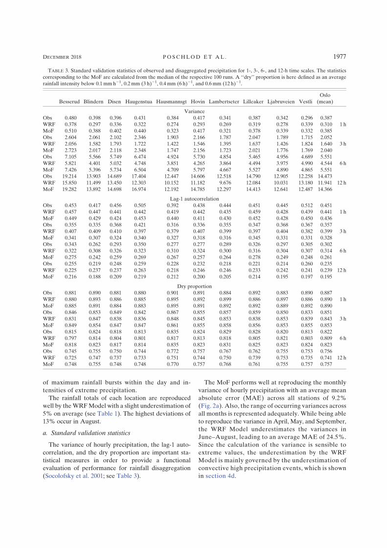
of maximum rainfall bursts within the day and in-

tensities of extreme precipitation.

The rainfall totals of each location are reproduced

well by theWRFModel with a slight underestimation of

5% on average (see Table 1). The highest deviations of

13% occur in August.

a. Standard validation statistics

The variance of hourly precipitation, the lag-1 auto-

correlation, and the dry proportion are important sta-

tistical measures in order to provide a functional

evaluation of performance for rainfall disaggregation

(Socolofsky et al. 2001; see Table 3).

The MoF performs well at reproducing the monthly

variance of hourly precipitation with an average mean

absolute error (MAE) across all stations of 9.2%

(Fig. 2a). Also, the range of occurring variances across

all months is represented adequately. While being able

to reproduce the variance in April, May, and September,

the WRF Model underestimates the variances in

June–August, leading to an average MAE of 24.5%.

Since the calculation of the variance is sensible to

extreme values, the underestimation by the WRF

Model is mainly governed by the underestimation of

convective high precipitation events, which is shown

in section 4d.

TABLE 3. Standard validation statistics of observed and disaggregated precipitation for 1-, 3-, 6-, and 12-h time scales. The statistics

corresponding to the MoF are calculated from the median of the respective 100 runs. A ‘‘dry’’ proportion is here defined as an average

rainfall intensity below 0.1mmh21, 0.2mm (3 h)21, 0.4mm (6 h)21, and 0.6mm (12 h)21.

Besserud Blindern Disen Haugenstua Hausmannsgt Hovin Lambertseter Lilleaker Ljabruveien Vestli

Oslo

(mean)

Variance

Obs 0.480 0.398 0.396 0.431 0.384 0.417 0.341 0.387 0.342 0.296 0.387

WRF 0.378 0.297 0.336 0.322 0.274 0.293 0.269 0.319 0.278 0.339 0.310 1 h

MoF 0.510 0.388 0.402 0.440 0.323 0.417 0.321 0.378 0.339 0.332 0.385

Obs 2.604 2.061 2.102 2.346 1.903 2.166 1.787 2.047 1.789 1.715 2.052

WRF 2.056 1.582 1.793 1.722 1.422 1.546 1.395 1.637 1.426 1.824 1.640 3 h

MoF 2.723 2.017 2.118 2.348 1.747 2.156 1.723 2.021 1.776 1.769 2.040

Obs 7.105 5.566 5.749 6.474 4.924 5.730 4.854 5.465 4.956 4.689 5.551

WRF 5.821 4.401 5.032 4.748 3.851 4.265 3.864 4.494 3.975 4.990 4.544 6 h

MoF 7.426 5.396 5.734 6.504 4.709 5.797 4.667 5.527 4.890 4.865 5.551

Obs 19.214 13.903 14.689 17.404 12.447 14.606 12.518 14.790 12.905 12.258 14.473

WRF 15.850 11.499 13.450 12.303 10.152 11.182 9.676 12.084 10.031 13.180 11.941 12 h

MoF 19.282 13.892 14.698 16.974 12.192 14.785 12.297 14.413 12.641 12.487 14.366

Lag-1 autocorrelation

Obs 0.453 0.417 0.456 0.505 0.392 0.438 0.444 0.451 0.445 0.512 0.451

WRF 0.457 0.447 0.441 0.442 0.419 0.442 0.435 0.459 0.428 0.439 0.441 1 h

MoF 0.449 0.429 0.424 0.453 0.440 0.411 0.430 0.452 0.428 0.450 0.436

Obs 0.355 0.335 0.368 0.421 0.316 0.336 0.355 0.347 0.368 0.367 0.357

WRF 0.407 0.409 0.410 0.397 0.379 0.407 0.399 0.397 0.404 0.382 0.399 3 h

MoF 0.341 0.307 0.324 0.340 0.327 0.318 0.316 0.345 0.331 0.331 0.328

Obs 0.343 0.262 0.293 0.350 0.277 0.277 0.289 0.326 0.297 0.305 0.302

WRF 0.322 0.308 0.326 0.323 0.310 0.324 0.300 0.316 0.304 0.307 0.314 6 h

MoF 0.275 0.242 0.259 0.269 0.267 0.257 0.264 0.278 0.249 0.248 0.261

Obs 0.255 0.219 0.248 0.259 0.228 0.232 0.218 0.221 0.214 0.260 0.235

WRF 0.225 0.237 0.237 0.263 0.218 0.246 0.246 0.233 0.242 0.241 0.239 12 h

MoF 0.216 0.188 0.209 0.219 0.212 0.200 0.205 0.214 0.195 0.197 0.195

Dry proportion

Obs 0.881 0.890 0.881 0.880 0.901 0.891 0.884 0.892 0.883 0.890 0.887

WRF 0.880 0.893 0.886 0.885 0.895 0.892 0.899 0.886 0.897 0.886 0.890 1 h

MoF 0.885 0.891 0.884 0.883 0.895 0.891 0.892 0.892 0.889 0.892 0.890

Obs 0.846 0.853 0.849 0.842 0.867 0.855 0.857 0.859 0.850 0.833 0.851

WRF 0.831 0.847 0.838 0.836 0.848 0.845 0.853 0.838 0.853 0.839 0.843 3 h

MoF 0.849 0.854 0.847 0.847 0.861 0.855 0.858 0.856 0.853 0.855 0.853

Obs 0.815 0.824 0.818 0.813 0.835 0.824 0.829 0.828 0.820 0.813 0.822

WRF 0.797 0.814 0.804 0.801 0.817 0.813 0.818 0.805 0.821 0.803 0.809 6 h

MoF 0.818 0.823 0.817 0.814 0.835 0.823 0.831 0.825 0.823 0.824 0.823

Obs 0.745 0.755 0.750 0.744 0.772 0.757 0.767 0.762 0.755 0.753 0.756

WRF 0.725 0.747 0.737 0.733 0.751 0.744 0.750 0.739 0.753 0.735 0.741 12 h

MoF 0.748 0.755 0.748 0.748 0.770 0.757 0.768 0.761 0.755 0.757 0.757

DECEMBER 2018 PO SCHLOD ET AL . 1977

The lag-1 autocorrelation represents the dependence

of the precipitation at two consecutive times. It is esti-

mated by the autocorrelation coefficient L1,

L15�N21

t51

R(t)2R� �

R(t1 1)2R� �

�N

t51

R(t)2R� �2

(5)

with R(t) as rainfall at time t of a series of length N with

mean precipitation R. Both methods perform well at

reconstructing this statistical measure at the 1-h time

scale with an average MAE across all stations of 5.8%

(WRF) and 6.0% (MoF).

However, the performance decreases for 3-h aggre-

gates with still acceptable MAEs of 13.2% (WRF) and

8.4% (MoF). At the aggregated time scales of 6 and 12h

the WRF Model outperforms the MoF with errors of

8.4% (WRF 6h) and 7.6% (WRF 12h) compared to

13.6% (MoF 6h) and 12.7% (MoF 12h). For all temporal

aggregations the MoF generally underestimates the lag-1

autocorrelation. This systematic underestimation was also

reported by Li et al. (2018) for the application in Singapore

and China. This can be explained by the MoF being un-

able to preserve the interday connectivity of precipitation

events. On average, 11.7 precipitation events per 6-month

period occurring overnight from one day to another are

observed. These events are defined as raining in the last

hour of the day and in the first hour of the following day.

The MoF can reconstruct 5.1 of these events leading to

a reduced autocorrelation coefficient L1, whereas the

WRF Model can reproduce 11.5 events per 6-month

period. For the aggregated time scales, this effect has a

greater impact on the value of L1 due to the higher

differences of rainfall at consecutive times entering in

Eq. (5).

To evaluate the reproduction of dry and wet times,

the dry proportion is calculated. It is important for the

further application of the disaggregated data that they

show no bias having too many dry or wet times. ‘‘Dry’’ is

defined as less than 0.1mmh21 mean rainfall intensity

due to the minimal resolution of the rain gauges. This is

necessary to provide consistency between the observa-

tional and WRF modeled datasets. For the aggregated

periods of 3, 6, and 12 h the threshold value cannot be

derived from scaling down the daily threshold for drizzle

of 1mmday21 (Sun et al. 2006) linearly, as the daily

threshold does not account for drizzle for every hour of

the 24h. Therefore, adapted thresholds of 0.2mm (3h),

0.4mm (6h), and 0.6mm (12 h) are introduced. The

MoF is able to reproduce these dry proportions with a

MAE of less than 0.5% for all time scales. TheMAEs of

theWRFModel amount to 0.7% (1h), 1.2% (3h), 1.6%

(6h), and 1.9% (12h). Hence, both models can preserve

FIG. 2. (a) Averagemonthly variance of hourly precipitation, (b) average of wet hours per month, (c) number, and (d) length of intraday

wet spells per rainy day, aggregated for all stations in Oslo. The range of variation across all stations is presented as box plots. The boxes

denote the interquartile range (IQR), which equals the six middle stations of 10 in total.

1978 JOURNAL OF HYDROMETEOROLOGY VOLUME 19

the percentage of wet and dry periods at the respective

time scales.

b. Wet hours per month, and number and length ofintraday wet spells

The amount of wet hours per month is considered to

assess the ability of both methods to capture the tem-

poral and site-specific variety of wet and dry periods.

The threshold value of 0.1mmh21 is again applied to

distinguish between wet and dry. The MoF is capable of

estimating the monthly sum of wet hours with an MAE

of 4.9% (see Fig. 2b) and of representing the range of

minima and maxima of all stations for each month. The

WRF Model also performs satisfyingly with an error of

9.6%, but overestimates the amount of wet hours in

April and underestimates it in August.

The number and length of intraday wet spells is of

great importance for the soil moisture conditions and

infiltration rates. Therefore, disaggregated precipitation

data preserving these characteristics are crucial for hy-

drological modeling and subsequent estimation of de-

sign floods (Haberlandt et al. 2008). An intraday wet

spell is defined by consecutive hours of precipitation $

0.1mmh21 within a day.

The number of intraday wet spells per rainy day (see

Fig. 2c) is reconstructed adequately with anMAE across

all stations and months of 4.5% (WRF) and 3.2% (MoF).

Both methods underestimate the maxima in August and

September, which are caused by just one station differ-

ing significantly during these two months (Vestli). The

corresponding durations of the intraday wet spells vary

across the whole summer season, with shorter, often

convective events during June–August and longer spells

in April, which are more frequently caused by stratiform

frontal systems.

The MoF can reproduce the duration with a MAE of

3.4% (Fig. 2d), whereas the WRF Model tends to ex-

aggerate the seasonal cycle, underestimating the dura-

tion in June–August and overestimating the duration in

April and September (MAE: 7.2%).

c. Spatial correlation

The preservation of the spatial correlation of each

rain gauge to its surrounding rain gauges is assessed by

calculating the Kendall rank coefficient t of all pairs of

stations for every month, as this measure does not rely

on any assumptions on the distribution or the linearity of

correlation.

The values for t for the station pairs of observed

hourly precipitation range from 0.40 to 0.86 (see Fig. 3).

The MoF fails to reconstruct this spatial correlation,

underestimating it systematically with a range from 0.14

to 0.52. TheWRFModel performs better at reproducing

the spatial correlation, but generally overestimates t by

10% on average, ranging from 0.60 to 0.92.

This can be explained by the neighboring conditions

of the grid cells leading to a too high similarity between

the cells and therefore too high correlation. Addition-

ally, the simulation of 9-km2 areal average precipitation

lowers the differences between the sites compared to the

point observations (Gregersen et al. 2013).

d. Timing of maximum rainfall bursts andexceedance probability of extremerainfall intensities

The MoF is able to reconstruct the timing of maxi-

mum rainfall bursts within a day very well for the mean

of all sites, as the daily cycle is quite similar at every

location (Fig. S3). The MAE for the median of the 100

runs for every single station and month amounts to

9.0%. The MoF reproduces the monthly cycle with the

interval of 12–17 h (see Fig. 4a) increasing from April to

June and decreasing from June to September due to

convective precipitation occurring more frequently in

the afternoon. The WRFModel is capable of rebuilding

the characteristics of the monthly cycle in the interval

of 12–17 h, but generally underestimates the percentage

of maximum rainfall bursts during 6–11h while over-

estimating it during 18–23 h (MAE: 15.5%). To set the

calculated MAEs into relation, they can be compared

to a uniform distribution of timings for every site (a

quarter of maximum bursts for each 6-h period), which

would result in a MAE of 13.3%. Therefore, the MoF

can clearly add value, whereas the WRF cannot re-

produce the overall timing.

In the following section, extreme events with an em-

pirical annual exceedance probability (AEP), 1 to occur

FIG. 3. Intersite Kendall rank correlation between the hourly

precipitation of all pairs of stations for every month.

DECEMBER 2018 PO SCHLOD ET AL . 1979

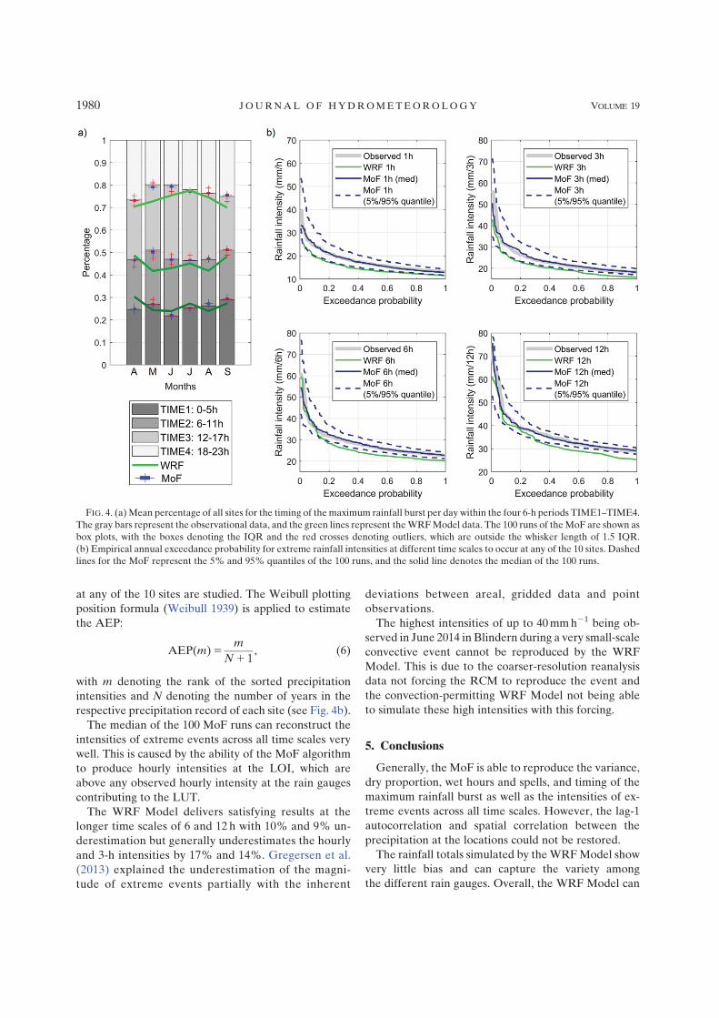
at any of the 10 sites are studied. The Weibull plotting

position formula (Weibull 1939) is applied to estimate

the AEP:

AEP(m)5m

N1 1, (6)

with m denoting the rank of the sorted precipitation

intensities and N denoting the number of years in the

respective precipitation record of each site (see Fig. 4b).

The median of the 100 MoF runs can reconstruct the

intensities of extreme events across all time scales very

well. This is caused by the ability of the MoF algorithm

to produce hourly intensities at the LOI, which are

above any observed hourly intensity at the rain gauges

contributing to the LUT.

The WRF Model delivers satisfying results at the

longer time scales of 6 and 12 h with 10% and 9% un-

derestimation but generally underestimates the hourly

and 3-h intensities by 17% and 14%. Gregersen et al.

(2013) explained the underestimation of the magni-

tude of extreme events partially with the inherent

deviations between areal, gridded data and point

observations.

The highest intensities of up to 40mmh21 being ob-

served in June 2014 in Blindern during a very small-scale

convective event cannot be reproduced by the WRF

Model. This is due to the coarser-resolution reanalysis

data not forcing the RCM to reproduce the event and

the convection-permitting WRF Model not being able

to simulate these high intensities with this forcing.

5. Conclusions

Generally, the MoF is able to reproduce the variance,

dry proportion, wet hours and spells, and timing of the

maximum rainfall burst as well as the intensities of ex-

treme events across all time scales. However, the lag-1

autocorrelation and spatial correlation between the

precipitation at the locations could not be restored.

The rainfall totals simulated by theWRFModel show

very little bias and can capture the variety among

the different rain gauges. Overall, the WRF Model can

FIG. 4. (a)Mean percentage of all sites for the timing of themaximum rainfall burst per day within the four 6-h periods TIME1–TIME4.

The gray bars represent the observational data, and the green lines represent theWRFModel data. The 100 runs of theMoF are shown as

box plots, with the boxes denoting the IQR and the red crosses denoting outliers, which are outside the whisker length of 1.5 IQR.

(b) Empirical annual exceedance probability for extreme rainfall intensities at different time scales to occur at any of the 10 sites. Dashed

lines for the MoF represent the 5% and 95% quantiles of the 100 runs, and the solid line denotes the median of the 100 runs.

1980 JOURNAL OF HYDROMETEOROLOGY VOLUME 19

reproduce the lag-1 autocorrelation, dry proportion, the

amount of wet hours, number and length of intraday wet

spells, and spatial correlation. The partial underestimation

of variance is mainly governed by the 9%–17% un-

derestimation of precipitation extremes, which can be

partially referred to the difference of grid-based simu-

lations to point measurements.

The performance of the MoF shows high suitability

for filling data gaps of subdaily historical records and

also disaggregation of data from rain gauges measuring

only daily precipitation. The preservation of hourly in-

tensities of heavy precipitation events makes the MoF

especially relevant for flood modeling of hydrological

systems with short response time. The MoF can also be

set up in minute resolution, which shows high potential

for applications within urban hydrology. However, it

requires a sufficient amount of high-resolution rainfall

observation stations and relies on historical data, restrict-

ing its scope of application regarding future scenarios.

The WRFModel has not only proven that it adds value

to the reanalysis data, but also has the ability to generate

hourly-resolution precipitation data, reproducing themain

characteristics of the observations. The biggest advantage

over statistical models is that the WRF Model can be ap-

plied in regions without observations. Due to its capability

of producing areal precipitation data the WRFModel can

serve as a data source for spatially distributed models.

Acknowledgments. The work has been carried out

within the SUPER project (250573) and the HYPRE

project (243942), both funded by the Research Council

of Norway and the ClimEx project funded by the Bavarian

State Ministry for the Environment and Consumer

Protection. The work has been supported by the European

Communities 7th Framework Programme Funding under

Grant Agreement 603629-ENV-2013-6.2.1-GLOBAQUA.

We acknowledge the precipitation data by the Norwe-

gian Meteorological Institute and the reanalysis data by

the National Centers for Environmental Prediction

(NCEP; data sources in references).

REFERENCES

Arnbjerg-Nielsen,K., P.Willems, J.Olsson, S. Beecham,A. Pathirana,

I. B. Gregersen, H. Madsen, and V. T. V. Nguyen, 2013: Impacts

of climate change on rainfall extremes and urban drainage sys-

tems: a review. Water Sci. Technol., 68, 16–28, https://doi.org/

10.2166/wst.2013.251.

Benestad, R. E., 2011: Updated temperature and precipitation

scenarios for Norwegian climate regions. Met.no Rep. 16/2011,

111 pp., https://www.met.no/publikasjoner/met-report/met-

report-2011.

Bennett, J. C., D. E. Robertson, P. G. D. Ward, H. A. Prasantha

Hapuarachchi, and Q. J. Wang, 2016: Calibrating hourly rainfall-

runoff models with daily forcings for streamflow forecasting

applications in meso-scale catchments. Environ. Modell. Soft-

ware, 76, 20–36, https://doi.org/10.1016/j.envsoft.2015.11.006.

Bruni, G., R. Reinoso, N. C. van de Giesen, F. H. L. R. Clemens,

and J. A. E. ten Veldhuis, 2015: On the sensitivity of urban

hydrodynamic modelling to rainfall spatial and temporal res-

olution. Hydrol. Earth Syst. Sci., 19, 691–709, https://doi.org/

10.5194/hess-19-691-2015.

Collins, W. D., and Coauthors, 2004: Description of the NCAR

Community Atmosphere Model (CAM 3.0). NCAR Tech.

Note NCAR/TN-4641STR, 214 pp., https://doi.org/10.5065/

D63N21CH.

Cristiano, E., M.-C. ten Veldhuis, and N. van de Giesen, 2017:

Spatial and temporal variability of rainfall and their effects

on hydrological response in urban areas – A review. Hydrol.

Earth Syst. Sci., 21, 3859–3878, https://doi.org/10.5194/hess-21-

3859-2017.

Dyrrdal, A. V., T. Skaugen, F. Stordal, and E. J. Førland, 2016:Estimating extreme areal precipitation in Norway from a

gridded dataset. Hydrol. Sci. J., 61, 483–494, https://doi.org/

10.1080/02626667.2014.947289.

——, F. Stordal, and C. Lussana, 2018: Evaluation of summer

precipitation from EURO-CORDEX fine-scale RCM simu-

lations over Norway. Int. J. Climatol., 38, 1661–1677, https://

doi.org/10.1002/joc.5287.

EEA, 2018: Europe coastline shapefile. European Environment

Agency, accessed 27 April 2018, https://www.eea.europa.eu/

data-and-maps/data/eea-coastline-for-analysis-1/gis-data/europe-

coastline-shapefile.

Flato, G., and Coauthors, 2013: Evaluation of climate models.

Climate Change 2013: The Physical Science Basis, T. F. Stocker

et al., Eds., Cambridge University Press, 741–866.

Geonorge, 2018: DTM 10 Terrengmodell (UTM32). Accessed

26 April 2018, https://kartkatalog.geonorge.no/metadata/

kartverket/dtm-10-terrengmodell-utm32/fd851873-f363-46f9-

9fc6-bb1b403575df.

Gregersen, I., H. Sørup, H. Madsen, D. Rosbjerg, P. Mikkelsen,

and K. Arnbjerg-Nielsen, 2013: Assessing future climatic

changes of rainfall extremes at small spatio-temporal scales.

Climatic Change, 118, 783–797, https://doi.org/10.1007/s10584-

012-0669-0.

Grell, G. A., and S. R. Freitas, 2014: A scale and aerosol aware

stochastic convective parameterization for weather and air

quality modeling. Atmos. Chem. Phys., 14, 5233–5250, https://

doi.org/10.5194/acp-14-5233-2014.

Haberlandt, U., A.-D. Ebner von Eschenbach, and I. Buchwald,

2008: A space-time hybrid hourly rainfall model for derived

flood frequency analysis. Hydrol. Earth Syst. Sci., 12, 1353–

1367, https://doi.org/10.5194/hess-12-1353-2008.

Hanssen-Bauer, I., and Coauthors, 2009: Klima i Norge 2100.

Bakgrunnsmateriale til NOU klimatilpassing. NCCS Rep.

2/2015, 204 pp.

Heikkilä, U., A. Sandvik, and A. Sorteberg, 2011: Dynamical

downscaling of ERA-40 in complex terrain using the WRF

regional climate model. Climate Dyn., 37, 1551–1564, https://

doi.org/10.1007/s00382-010-0928-6.

Hong, S.-Y., and J.-O. J. Lim, 2006: The WRF single-moment

6-class microphysics scheme (WSM6). J. Korean Meteor. Soc.,

42 (2), 129–151.

——, Y. Noh, and J. Dudhia, 2006: A new vertical diffusion package

with an explicit treatment of entrainment processes.Mon. Wea.

Rev., 134, 2318–2341, https://doi.org/10.1175/MWR3199.1.

Jimenez, P. A., J. Dudhia, J. F. Gonzalez–Rouco, J. Navarro, J. P.

Montavez, and E. Garcia–Bustamante, 2012: A revised scheme

DECEMBER 2018 PO SCHLOD ET AL . 1981

for the WRF surface layer formulation. Mon. Wea. Rev., 140,

898–918, https://doi.org/10.1175/MWR-D-11-00056.1.

Kottek,M., J.Grieser, C. Beck, B.Rudolf, andF.Rubel, 2006:World

Map of the Köppen-Geiger climate classification updated. Me-

teor. Z., 15, 259–263, https://doi.org/10.1127/0941-2948/2006/0130.

Koutsoyiannis, D., 2003: Rainfall disaggregation methods: Theory

and applications. Proc. Workshop on Statistical and Math-

ematical Methods for Hydrological Analysis, Rome, Italy,

University of Rome, 1–23, http://itia.ntua.gr/getfile/570/1/

documents/2003RainDisag.pdf.

Lall, U., and A. Sharma, 1996: A nearest neighbor bootstrap for

time series resampling. Water Resour. Res., 32, 679–693,https://doi.org/10.1029/95WR02966.

Li, X., and Coauthors, 2018: Three resampling approaches based

on method of fragments for daily-to-subdaily precipitation

disaggregation. Int. J. Climatol., 38, e1119–e1138, https://

doi.org/10.1002/joc.5438.

Mayer, S., C. FoxMaule, S. Sobolowski, O. B. Christensen, H. J. D.

Sørup, M. A. Sunyer, K. Arnbjerg-Nielsen, and I. Barstad,

2015: Identifying added value in high-resolution climate sim-

ulations over Scandinavia. Tellus, 67A, 24941, https://doi.org/

10.3402/tellusa.v67.24941.

NCEP, 2000: NCEP FNLOperationalModel Global Tropospheric

Analyses, continuing from July 1999. Research Data Archive

at the National Center for Atmospheric Research, Com-

putational and Information Systems Laboratory, accessed

22 February 2018, https://doi.org/10.5065/D6M043C6.

NMI, 2018: eKlima. Norwegian Meteorological Institute, accessed

12 February 2018, http://eKlima.met.no.

Ochoa-Rodriguez, S., and Coauthors, 2015: Impact of spatial and

temporal resolution of rainfall inputs on urban hydrodynamic

modelling outputs: A multi-catchment investigation. J. Hydrol.,

531, 389–407, https://doi.org/10.1016/j.jhydrol.2015.05.035.

Park, S., and C. S. Bretherton, 2009: The University of Washington

shallow convection and moist turbulence schemes and their

impact on climate simulations with the Community Atmo-

sphere Model. J. Climate, 22, 3449–3469, https://doi.org/

10.1175/2008JCLI2557.1.

Powers, J. G., J. B. Klemp, W. C. Skamarock, C. A. Davis,

J. Dudhia, D. O. Gill, J. L. Coen, and D. J. Gochis, 2017: The

Weather Research and Forecasting (WRF)Model: Overview,

system efforts, and future directions.Bull. Amer. Meteor. Soc.,

98, 1717–1737, https://doi.org/10.1175/BAMS-D-15-00308.1.

Prein, A. F., and Coauthors, 2015: A review on regional

convection-permitting climate modeling: Demonstrations,

prospects, and challenges. Rev. Geophys., 53, 323–361, https://

doi.org/10.1002/2014RG000475.

Pui, A., A. Sharma, R. Mehrotra, B. Sivakumar, and E. Jeremiah,

2012: A comparison of alternatives for daily to sub-daily

rainfall disaggregation. J. Hydrol., 470–471, 138–157, https://

doi.org/10.1016/j.jhydrol.2012.08.041.

Reynolds, J. E., S.Halldin, C.Y.Xu, J. Seibert, andA.Kauffeldt, 2017:

Sub-daily runoff predictions using parameters calibrated on the

basis of data with a daily temporal resolution. J. Hydrol., 550,

399–411, https://doi.org/10.1016/j.jhydrol.2017.05.012.

Sharma, A., and S. Srikanthan, 2006: Continuous rainfall simu-

lation: A nonparametric alternative. 30th Hydrology & Wa-

ter Resources Symp.: Past, Present & Future, Launceston,

Australia, Institution of Engineers, 86–91.

Sillmann, J., and Coauthors, 2017: Understanding, modeling and

predicting weather and climate extremes: Challenges and op-

portunities. Wea. Climate Extremes, 18, 65–74, https://doi.org/10.1016/j.wace.2017.10.003.

Skamarock, W., and J. Klemp, 2008: A time-split nonhydrostatic

atmospheric model for weather research and forecasting ap-

plications. J. Comput. Phys., 227, 3465–3485, https://doi.org/10.1016/j.jcp.2007.01.037.

Socolofsky, S., E. E. Adams, and D. Entekhabi, 2001: Disaggre-

gation of daily rainfall for continuous watershed modeling.

J. Hydrol. Eng., 6, 300–309, https://doi.org/10.1061/(ASCE)

1084-0699(2001)6:4(300).

Sun, Y., S. Solomon, A. Dai, and R.W. Portmann, 2006: How often

does it rain? J. Climate, 19, 916–934, https://doi.org/10.1175/JCLI3672.1.

Tabari, H., and Coauthors, 2016: Local impact analysis of climate

change on precipitation extremes: Are high-resolution cli-

mate models needed for realistic simulations? Hydrol.

Earth Syst. Sci., 20, 3843–3857, https://doi.org/10.5194/hess-

20-3843-2016.

Tewari, M., and Coauthors, 2004: Implementation and verification

of the unified NOAH land surface model in the WRF Model.

20th Conf. on Weather Analysis and Forecasting/16th Conf. on

Numerical Weather Prediction, Seattle, WA, Amer. Meteor.

Soc., 14.2a, https://ams.confex.com/ams/84Annual/techprogram/

paper_69061.htm.

Tjelta, T., and J. Mamen, 2014: Climate trends and variability of

rain rate derived from long-term measurements in Norway.

Radio Sci., 49, 788–797, https://doi.org/10.1002/2014RS005477.

Weibull, W., 1939: A statistical theory of the strength of materials.

Ing. Vetensk. Akad. Handl., 151, 1–45.

Westra, S., R. Mehrotra, A. Sharma, and R. Srikanthan, 2012:

Continuous rainfall simulation: 1. A regionalized subdaily

disaggregation approach. Water Resour. Res., 48, W01535,

https://doi.org/10.1029/2011WR010489.

1982 JOURNAL OF HYDROMETEOROLOGY VOLUME 19

116

Conclusion and Outlook 117

3 Conclusion and Outlook

The present thesis covers a wide range of hydrometeorological processes on different tem-

poral and spatial scales. The following chapter summarizes the main findings of the publica-

tions and, in this context, answers the research questions posed in Section 1.3. Furthermore,

based on these findings, recommendations for similar studies will be given and future devel-

opments in regional climate modelling will be discussed.

• RQ1: Can the high-resolution CRCM5 ensemble simulate hydrometeorogical pro-

cesses and extremes over Europe?

All three publications featuring the CRCM5-LE included a careful evaluation of the model per-

formance applying observational data and have, therefore, shown that regional climate models

are able to capture many features of the hydrometeorology over Europe. Nevertheless, in all

publications deviations between observations and simulations occurred, which were dealt with

in different ways. In Publication I (Poschlod et al., 2020c), no bias adjustment was applied. The

regional climate ensemble could reproduce extreme rainfall intensity in large parts of Europe.

However, over complex terrain and regions with high convective activity, the CRCM5-LE un-

derestimated short-duration extremes. Within Publication II, the spatial pattern of temperature

and precipitation was captured by the CRCM5 over southern Norway revealing that annual

rainfall was overestimated by the climate model. The other variables used, such as soil mois-

ture and snow melt, could not be validated area-wide due to missing observations. As com-

pound events were investigated, BA should have been multivariate, but could not be carried

out due to the lack of data. This problem was therefore circumvented by choosing a quantile-

based framework, which focuses on the joint occurrence of the driving variables rather than on

their absolute values.

• RQ2: Can the hydrological ensemble (WaSiM driven by CRCM5) reproduce the sea-

sonality of river runoff in Bavaria? And how will it be affected by climate change?

For the investigation of the seasonality of mean flows in Bavaria, the hydrological impact model

WaSiM was applied. In order to drive this model, biases of temperature, precipitation, humidity

and winds were adjusted. Although observations also suffer from measurement errors. Publi-

cation III (Poschlod et al., 2020b) has shown from a hydrological point of view, that observa-

tional rainfall undercatch is largely affecting the quality of runoff simulations in areas, where

snow melt significantly contributes to runoff generation. Especially solid precipitation is under-

estimated by rain gauges, which is well-known for decades (Richter, 1995; Sevruk, 1985).

When adjusting the bias of a RCM, the reference data should be first corrected for undercatch.

In the largest part of the study area, however, the resulting simulated runoff of the processing

chain can reproduce the observed mean flows and their seasonality very well. The changing

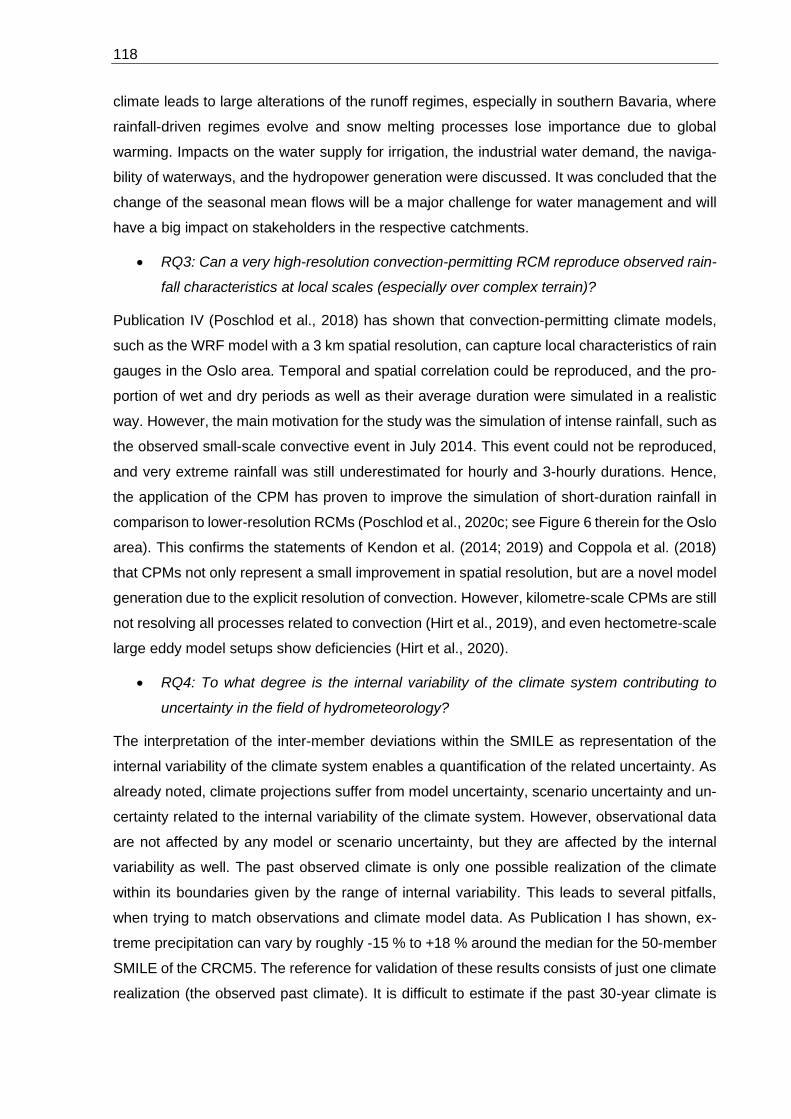
118

climate leads to large alterations of the runoff regimes, especially in southern Bavaria, where

rainfall-driven regimes evolve and snow melting processes lose importance due to global

warming. Impacts on the water supply for irrigation, the industrial water demand, the naviga-

bility of waterways, and the hydropower generation were discussed. It was concluded that the

change of the seasonal mean flows will be a major challenge for water management and will

have a big impact on stakeholders in the respective catchments.

• RQ3: Can a very high-resolution convection-permitting RCM reproduce observed rain-

fall characteristics at local scales (especially over complex terrain)?

Publication IV (Poschlod et al., 2018) has shown that convection-permitting climate models,

such as the WRF model with a 3 km spatial resolution, can capture local characteristics of rain

gauges in the Oslo area. Temporal and spatial correlation could be reproduced, and the pro-

portion of wet and dry periods as well as their average duration were simulated in a realistic

way. However, the main motivation for the study was the simulation of intense rainfall, such as

the observed small-scale convective event in July 2014. This event could not be reproduced,

and very extreme rainfall was still underestimated for hourly and 3-hourly durations. Hence,

the application of the CPM has proven to improve the simulation of short-duration rainfall in

comparison to lower-resolution RCMs (Poschlod et al., 2020c; see Figure 6 therein for the Oslo

area). This confirms the statements of Kendon et al. (2014; 2019) and Coppola et al. (2018)

that CPMs not only represent a small improvement in spatial resolution, but are a novel model

generation due to the explicit resolution of convection. However, kilometre-scale CPMs are still

not resolving all processes related to convection (Hirt et al., 2019), and even hectometre-scale

large eddy model setups show deficiencies (Hirt et al., 2020).

• RQ4: To what degree is the internal variability of the climate system contributing to

uncertainty in the field of hydrometeorology?

The interpretation of the inter-member deviations within the SMILE as representation of the

internal variability of the climate system enables a quantification of the related uncertainty. As

already noted, climate projections suffer from model uncertainty, scenario uncertainty and un-

certainty related to the internal variability of the climate system. However, observational data

are not affected by any model or scenario uncertainty, but they are affected by the internal

variability as well. The past observed climate is only one possible realization of the climate

within its boundaries given by the range of internal variability. This leads to several pitfalls,

when trying to match observations and climate model data. As Publication I has shown, ex-

treme precipitation can vary by roughly -15 % to +18 % around the median for the 50-member

SMILE of the CRCM5. The reference for validation of these results consists of just one climate

realization (the observed past climate). It is difficult to estimate if the past 30-year climate is

Conclusion and Outlook 119

close to the edges of the boundaries of internal variability or if it reflects a rather probable

realization.

Having this in mind, also the bias adjustment of climate model data has to be critically re-

viewed, especially for processes, which are highly variable, such as precipitation and winds. A

“typical” impact-related model chain features a bias adjustment of the climate model data in

relation to observation-based reference data, often carried out via quantile mapping or quantile

delta mapping (Cannon et al., 2015; Willkofer et al., 2018). Thereby, the physically-based re-

sults of the climate model are adjusted with scaling factors that force the distribution of each

adjusted variable to the distribution of the observations. However, the internal variability of the

observations and the climate model should be taken into account (Zscheischler et al., 2019).

The variability is varying for different regions of the distributions, with the highest variability in

the tails (e.g. Aalbers et al., 2018; Poschlod et al., 2020c). Hence the scaling factors of the

bias adjustment should allow more degrees of freedom according to the range of internal var-

iability in order to carry out a “relaxed bias adjustment”. This issue has been discussed by

Chen et al. (2016) and Kim et al. (2016), but is still rarely implemented.

Another crucial impact of the missing representation of internal variability within observations

can be too high confidence in the estimation of occurrence probability of extreme events. Leg-

islative boundaries and engineering guidelines are often based on return levels. A common

design parameter for flood protection is HF100, a flood discharge which statistically occurs

once in 100 years (LfU, 2020). The design rainfall for roof drainage is a rain event with a sta-

tistical frequency of 5 years and a rain duration of 5 minutes (Röder, 2008). The estimation of

these return levels are based on observations, where extreme value distributions are fitted to

the empirical distributions. Thereby, a confidence interval can be calculated for the respective

return level for the requested confidence level α. However, this confidence interval describes

exclusively the uncertainty that exists on the basis of the fit of the extreme value distribution to

the empirical distribution. Uncertainty due to internal variability affecting the observations

providing the empirical distribution is not considered. Almost no return level assessment dis-

cusses these uncertainties due to internal variability or even tries to quantify them. Publication

I (Poschlod et al., 2020c) has proven that internal variability plays a major role for the estima-

tion of rainfall return levels, although the application of a theoretical extreme value distribution

does not fully smooth out the variability in the samples. In addition, Publication II (Poschlod et

al., 2020a) has shown that the joint occurrence of flood drivers is also highly variable, which

leads to an even bigger impact of internal variability within the non-linear system of river hy-

drology. This will be further analysed for the study area of hydrological Bavaria applying the

runoff data of the ClimEx project.

Research questions RQ5 and RQ6 shall be answered collectively.

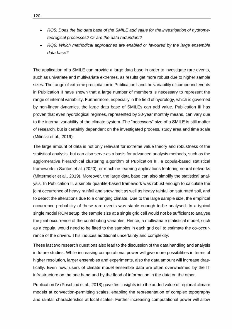
120

• RQ5: Does the big data base of the SMILE add value for the investigation of hydrome-

teorogical processes? Or are the data redundant?

• RQ6: Which methodical approaches are enabled or favoured by the large ensemble

data base?

The application of a SMILE can provide a large data base in order to investigate rare events,

such as univariate and multivariate extremes, as results get more robust due to higher sample

sizes. The range of extreme precipitation in Publication I and the variability of compound events

in Publication II have shown that a large number of members is necessary to represent the

range of internal variability. Furthermore, especially in the field of hydrology, which is governed

by non-linear dynamics, the large data base of SMILEs can add value. Publication III has

proven that even hydrological regimes, represented by 30-year monthly means, can vary due

to the internal variability of the climate system. The “necessary” size of a SMILE is still matter

of research, but is certainly dependent on the investigated process, study area and time scale

(Milinski et al., 2019).

The large amount of data is not only relevant for extreme value theory and robustness of the

statistical analysis, but can also serve as a basis for advanced analysis methods, such as the

agglomerative hierarchical clustering algorithm of Publication III, a copula-based statistical

framework in Santos et al. (2020), or machine-learning applications featuring neural networks

(Mittermeier et al., 2019). Moreover, the large data base can also simplify the statistical anal-

ysis. In Publication II, a simple quantile-based framework was robust enough to calculate the

joint occurrence of heavy rainfall and snow melt as well as heavy rainfall on saturated soil, and

to detect the alterations due to a changing climate. Due to the large sample size, the empirical

occurrence probability of these rare events was stable enough to be analysed. In a typical

single model RCM setup, the sample size at a single grid cell would not be sufficient to analyse

the joint occurrence of the contributing variables. Hence, a multivariate statistical model, such

as a copula, would need to be fitted to the samples in each grid cell to estimate the co-occur-

rence of the drivers. This induces additional uncertainty and complexity.

These last two research questions also lead to the discussion of the data handling and analysis

in future studies. While increasing computational power will give more possibilities in terms of

higher resolution, larger ensembles and experiments, also the data amount will increase dras-

tically. Even now, users of climate model ensemble data are often overwhelmed by the IT

infrastructure on the one hand and by the flood of information in the data on the other.

Publication IV (Poschlod et al., 2018) gave first insights into the added value of regional climate

models at convection-permitting scales, enabling the representation of complex topography

and rainfall characteristics at local scales. Further increasing computational power will allow

Conclusion and Outlook 121

for higher-resolution SMILEs and MMEs, up to convection-permitting scales. This will create

the data base to explore the internal variability and model uncertainty of small scale features

and short-duration events, such as extreme rainfall at sub-hourly time scales, which is relevant

for the dimensioning of roofs, urban drainage systems and also the trigger for mass move-

ments such as flash floods and splash erosion. The development towards RESMs will also

increase the number of simulated processes and thus resulting variables. The methods of

analysis, therefore, have to evolve as well.

122

References 123

References

Aalbers, E. E., Lenderink, G., van Meijgaard, E., van den Hurk, B. J. J. M. (2018): Local-scale

changes in mean and heavy precipitation in western Europe, climate change or internal varia-

bility? Clim. Dynam., 50, 4745–4766.

Addor, N., Rössler, O., Köplin, N., Huss, M., Weingartner, R., Seibert, J. (2014): Robust

changes and sources of uncertainty in the projected hydrological regimes of Swiss catchments.

Water Resour. Res., 50, 7541–7562.

AMS (American Meteorological Society; Ed.): Journal of Hydrometeorology. URL: https://jour-

nals.ametsoc.org/jhm (accessed on 18.07.2020).

Behrangi, A., Gardner, A., Reager, J. T., Fisher, J. B., Yang, D., Human, G. J., Adler, R. F.

(2018): Using GRACE to Estimate Snowfall Accumulation and Assess Gauge Undercatch Cor-

rections in High Latitudes. J. Clim., 31, 8689–8704.

Bender, M. A., Knutson, T. R., Tuleya, R. E., Sirutis, J. J., Vecchi, G. A., Garner, S. T., Held,

I. M. (2010): Modeled Impact of Anthropogenic Warming on the Frequency of Intense Atlantic

Hurricanes. Science, 327, 454–458.

Benoit, R., Schär, C., Binder, P., Chamberland, S., Davies, H. C., Desgagné, M., Girard, C.,

Keil, C., Kouwen, N., Luthi, D., Maric, D., Müller, E., Pellerin, P., Schmidli, J., Schubiger, F.,

Schwierz, C., Sprenger, M., Walser, A., Willemse, S., Yu, W., Zala, E. (2002): The real-time

ultra finescale forecast support during the special observing period of the MAP. Bull. Amer.

Meteor. Soc., 83, 85–109.

Berg, P., Christensen, O. B., Klehmet, K., Lenderink, G., Olsson, J., Teichmann, C., Yang, W.

(2019): Summertime precipitation extremes in a EURO-CORDEX 0.11° ensemble at an hourly

resolution. Nat. Haz. Earth Sys. Sci., 19, 4, 957–971.

Beven, K. (2006): A manifesto for the equifinality thesis. J. Hydrol., 320, 18–36.

Box, G. E. P. (1976): Science and statistics. Journal of the American Statistical Association,

71, 356, 791–799.

Briggs, P. R., Cogley, J. G. (1996): Topographic bias in mesoscale precipitation networks. J.

Clim., 9, 1, 205–218.

Cannon, A. J., Sobie, S. R., Murdock, T. Q. (2015): Bias correction of simulated precipitation

by quantile mapping: how well do methods preserve relative changes in quantiles and ex-

tremes? J. Clim., 28, 17, 6938–6959.

124

Cannon, A.J. (2018): Multivariate quantile mapping bias correction: an N-dimensional proba-

bility density function transform for climate model simulations of multiple variables. Clim. Dyn.,

50, 31–49.

Caya, D., Laprise, R. (1999): A semi‐implicit, semi‐Lagrangian regional climate model: The

Canadian RCM. Monthly Weather Review, 127, 341–362.

Chen, J., Brissette, F. P., Poulin, A., Leconte, R. (2011): Overall uncertainty study of the hy-

drological impacts of climate change for a Canadian watershed. Water Resour. Res., 47,

W12509.

Chen, J., St-Denis, B. G., Brissette, F. P., Lucas-Picher, P. (2016): Using Natural Variability as

a Baseline to Evaluate the Performance of Bias Correction Methods in Hydrological Climate

Change Impact Studies. J. Hydrometeor., 17, 2155–2174.

Chen, T., Ren, L., Yuan, F., Yang, X., Jiang, S., Tang, T., Liu, Y., Zhao, C., Zhang, L. (2017):

Comparison of spatial interpolation schemes for rainfall data and application in hydrological

modeling. Water, 9, 5, 342.

Christensen, J. H., Machenhauer, B., Jones, R. G., Schär, C., Ruti, P. M., Castro, M., Visconti,

G. (1997): Validation of present day regional climate simulations over Europe: LAM simulations

with observed boundary conditions. Clim. Dyn., 13, 7‐8, 489–506.

Collier, E., Mölg, T. (2020): BAYWRF: a convection-resolving, present-day climatological at-

mospheric dataset for Bavaria. Earth Syst. Sci. Data Discuss., in review.

Collins, M., Booth, B. B., Bhaskaran, B., Harris, G. R., Murphy, J. M., Sexton, D. M., Webb, M.

J. (2011): Climate model errors, feedbacks and forcings: a comparison of perturbed physics

and multi-model ensembles. Clim. Dyn., 36, 9-10, 1737–1766.

Copernicus GmbH (Ed.): Earth System Science Data. URL: https://www.earth-system-sci-

ence-data.net/ (accessed on 18.07.2020).

Coppola, E., Sobolowski, S., Pichelli, E., Raffaele, F., Ahrens, B., Anders, I., Ban, N., Bastin,

S., Belda, M., Belušić, D., Caldas-Alvarez, A., Cardoso, R. M., Davolio, S., Dobler, A., Fernan-

dez, J., Fita, L., Fumiere, Q., Giorgi, F., Goergen, K., Güttler, I., Halenka, T., Heinzeller, D.,

Hodnebrog, Ø., Jacob, D., Kartsios, S., Katragkou, E., Kendon, E., Khodayar, S., Kunstmann,

H., Knist, S., Lavín-Gullón, A., Lind, P., Lorenz, T., Maraun, D., Marelle, L., van Meijgaard, E.,

Milovac, J., Myhre, G., Panitz, H.-J., Piazza, M., Raffa, M., Raub, T., Rockel, B., Schär, C.,

Sieck, K., Soares, P. M. M., Somot, S., Srnec, L., Stocchi, P., Tölle, M. H., Truhetz, H., Vautard,

R., de Vries, H., Warrach-Sagi, K. (2018): A first-of-its-kind multi-model convection permitting

ensemble for investigating convective phenomena over Europe and the Mediterranean, Clim.

Dyn., 55, 3–34.

References 125

Courant, R., Friedrichs, K., Lewy, H. (1967): On the partial difference equations of mathemat-

ical physics. IBM journal of Research and Development, 11, 2, 215–234.

Davies, T. (2014): Lateral boundary conditions for limited area models. Q. J. R. Meteorol. Soc.,

140, 185–196.

Denis, B., Laprise, R., Caya, D. (2003): Sensitivity of a regional climate model to the spatial

resolution and temporal updating frequency of the lateral boundary conditions. Clim. Dyn., 20,

107–126.

Déqué, M., Rowell, D. P., Lüthi, D., Giorgi, F., Christensen, J. H., Rockel, B., Jacob, D., Kjell-

ström, E., De Castro, M., van den Hurk, B. J. J. M. (2007): An intercomparison of regional

climate simulations for Europe: assessing uncertainties in model projections. Clim. Change,

81, 53–70.

Deser, C., Phillips, A., Bourdette, V., Teng, H. (2012): Uncertainty in climate change projec-

tions: the role of internal variability. Clim. Dyn., 38, 3-4, 527–546.

Dickinson, R. E., Errico, R. M., Giorgi, F., Bates, G. T. (1989): A regional climate model for the

western United States. Clim. Change, 15, 383–422.

Dobler, C., Hagemann, S., Wilby, R., Stötter, J. (2012): Quantifying different sources of uncer-

tainty in hydrological projections in an Alpine watershed. Hydrol. Earth Syst. Sci., 16, 4343–

4360.

Döscher, R., Wyser, K., Meier, H. E. M., Qian, M., Redler., R. (2010): Quantifying Arctic Con-

tributions to Climate Predictability in a Regional Coupled Ocean-Ice-Atmosphere Model. Clim.

Dyn., 34, 1157–1176.

Dosio, A. (2016): Projections of climate change indices of temperature and precipitation from

an ensemble of bias-adjusted high-resolution EURO-CORDEX regional climate models. Jour-

nal of Geophysical Research: Atmospheres, 121, 10, 5488–5511.

Dubois, C., Somot, S., Calmanti, S., Carillo, A., Déqué, M., Dell’Aquilla, A., Elizalde, A. (2012):

Future Projections of the Surface Heat and Water Budgets of the Mediterranean Sea in an

Ensemble of Coupled Atmosphere-Ocean Regional Climate Models. Clim. Dyn., 39, 1859–

1884.

Ducrocq, V., Ricard, D., Lafore, J. P., Orain, F. (2002): Storm-scale numerical rainfall predic-

tion for five precipitating events over France: on the importance of the initial humidity field.

Weather Forecast, 17, 1236–1256.

Ehret, U., Zehe, E., Wulfmeyer, V., Warrach-Sagi, K, Liebert, J. (2012): Should we apply bias

correction to global and regional climate model data? Hydrol. Earth Syst. Sci., 16, 3391–3404.

126

Ellis, E. C. (2017): Physical geography in the Anthropocene. Progress in Physical Geography:

Earth and Environment, 41, 5, 525–532.

Elsevier (Ed.): Weather and Climate Extremes. URL: https://www.sciencedirect.com/jour-

nal/weather-and-climate-extremes/about/aims-and-scope (accessed on 18.07.2020).

Flato, G. M. (2011): Earth system models: an overview. Wiley Interdisciplinary Reviews: Clim.

Change, 2, 6, 783–800.

Flato, G., J. Marotzke, B. Abiodun, P. Braconnot, S.C. Chou, W. Collins, P. Cox, F. Driouech,

S. Emori, V. Eyring, C. Forest, P. Gleckler, E. Guilyardi, C. Jakob, V. Kattsov, C. Reason and

M. Rummukainen, (2013): Evaluation of Climate Models. In: Stocker, T.F., D. Qin, G.-K. Platt-

ner, M. Tignor, S.K. Allen, J. Boschung, A. Nauels, Y. Xia, V. Bex and P.M. Midgley (Eds.):

Climate Change 2013: The Physical Science Basis. Contribution of Working Group I to the

Fifth Assessment Report of the Intergovernmental Panel on Climate Change Cambridge Uni-

versity Press, Cambridge, United Kingdom and New York, NY, USA.

François, B., Vrac, M., Cannon, A. C., Robin, Y., Allard, D. (2020): Multivariate bias corrections

of climate simulations: which benefits for which losses? Earth Syst. Dynam., 11, 537–562.

Gampe, D., Nikulin, G., Ludwig, R. (2016): Using an ensemble of regional climate models to

assess climate change impacts on water scarcity in European river basins. Science of the Total

Environment, 573, 1503–1518.

Gampe, D., J. Schmid, R. Ludwig (2019): Impact of Reference Dataset Selection on RCM

Evaluation, Bias Correction, and Resulting Climate Change Signals of Precipitation. J. Hydro-

meteor., 20, 1813–1828.

Gao, X., Pal, J. S., Giorgi, F. (2006): Projected changes in mean and extreme precipitation

over the Mediterranean region from high resolution double nested RCM simulations. Geophys.

Res. Lett., 33, L03706.

Gibelin, A. L., Déqué, M. (2003): Anthropogenic climate change over the Mediterranean region

simulated by a global variable resolution model. Clim. Dyn., 20, 327–339.

Giorgi, F. (2019): Thirty Years of Regional Climate Modeling: Where Are We and Where Are

We Going next? Journal of Geophysical Research: Atmospheres, 124, 5696–5723.

Giorgi, F., Bates, G. T. (1989): The climatological skill of a regional model over complex terrain.

Mon. Wea. Rev., 117, 2325–2347.

Giorgi, F., Bates, G. T., Nieman, S. J. (1993): The multi‐year surface climatology of a regional

atmospheric model over the western United States. Journal of Climate, 6, 75–95.

Giorgi, F., Gao, X. J. (2018): Regional Earth system modeling: Review and future directions.

Atmospheric and Oceanic Science Letters, 11, 189–197.

References 127

Giorgi, F., Gutowski, W. L. (2015): Regional dynamical downscaling and the CORDEX initia-

tive. Annual Review of Environment and Resources, 40, 467–490.

Grossi, G., Lendvai, A., Peretti, G., Ranzi, R. (2017): Snow Precipitation Measured by Gauges:

Systematic Error Estimation and Data Series Correction in the Central Italian Alps. Water, 9,

461.

Gudmundsson, L., Bremnes, J. B., Haugen, J. E., Engen-Skaugen, T. (2012): Technical Note:

Downscaling RCM precipitation to the station scale using statistical transformations – a com-

parison of methods. Hydrol. Earth Syst. Sci., 16, 3383–3390.

Hank, T. B., Bach, H., Mauser, W. (2015): Using a Remote Sensing-Supported Hydro-Agroe-

cological Model for Field-Scale Simulation of Heterogeneous Crop Growth and Yield: Applica-

tion for Wheat in Central Europe. Remote Sens., 7, 3934–3965.

Hao, Z., Singh, V.P., Hao, F. (2018): Compound extremes in hydroclimatology: a review. Wa-

ter, 10, 6, 718.

Hattermann, F. F., Krysanova, V., Gosling, S., Dankers, R., Daggupati, P., Donnelly, C., Flörke,

M., Huang, S., Motovilov, Y., Buda, S., Yang, T., Müller, C., Leng, G., Tang, Q., Portmann, F.

T., Hagemann, S., Gerten, D., Wada, Y., Masaki, Y., Alemayehu, T., Satoh, Y., Samaniego, L.

(2017): Cross-scale intercomparison of climate change impacts simulated by regional and

global hydro-logical models in eleven large river basins. Clim. Change, 141, 561–576.

Hattermann, F., Vetter, T., Breuer, L., Su, B., Daggupati, P., Donnelly, C., Fekete, B., Flörke,

F., Gosling, S. N., Hoffmann, P., Liersch, S., Masaki, Y., Motovilov, Y., Müller, C., Samaniego,

L., Stacke, T., Wada, Y., Yang, T., Krysnaova, V. (2018): Sources of uncertainty in hydrological

climate impact assessment: a cross-scale study. Environ. Res. Lett., 13, 1, 015006.

Hausfather, Z., Drake, H. F., Abbott, T., Schmidt, G. A. (2020): Evaluating the performance of

past climate model projections. Geophys. Res. Lett., 47, e2019GL085378.

Hawkins, E., Sutton, R. (2009): The potential to narrow uncertainty in regional climate predic-

tions. Bulletin of the American Meteorological Society, 90, 8, 1095–1107.

Her, Y., Yoo, S. H., Cho, J., Hwang, S., Jeong, J., Seong, C. (2019): Uncertainty in hydrological

analysis of climate change: Multi-parameter vs. multi-GCM ensemble predictions. Sci. Rep.,

9, 1–22.

Hewitt, C. D., Senior, C. A., Mitchell, J. F. B. (2001): The impact of dynamic sea-ice on the

climatology and climate sensitivity of a GCM: a study of past, present, and future climates.

Clim. Dyn., 17, 655–668.

128

Hirt, M., Rasp, S., Blahak, U., Craig, G. C. (2019): Stochastic Parameterization of Processes

Leading to Convective Initiation in Kilometer-Scale Models. Mon. Wea. Rev., 147, 11, 3917–

3934.

Hirt, M., Craig, G. C., Schäfer, S. A. K., Savre, J., Heinze, R. (2020): Cold‐pool‐driven convec-

tive initiation: using causal graph analysis to determine what convection‐permitting models are

missing. Q. J. R. Meteorol. Soc., 146, 2205–2227.

Houghton, J. T., Jenkins, G. J., Ephraums, J. J. (Eds.) (1990): Climate Change: The IPCC

Scientific Assessment. Report Prepared for the IPCC by Working Group 1. Cambridge, Cam-

bridge University Press, 358pp.

van den Hurk, B. J. J. M., van Meijgaard, E., de Valk, P., van Heeringen, K.-J., Gooijer, J.

(2015): Analysis of a compounding surge and precipitation event in the Netherlands. Environ.

Res. Lett., 10, 035001.

Im, E. S., Park, E.‐H., Kwon, W.‐T., Giorgi, F. (2008): Multi‐decadal scenario simulation over

Korea using a RegCM3 one‐way doublenested system. Part 2: Future climate projection

(2021‐2050). Clim. Dyn., 30, 239–254.

Jerez, S., López‐Romero, J. M., Turco, M., Lorente‐Plazas, R., Gómez‐Navarro, J. J., Jimé-

nez‐Guerrero, P., Montávez, J. P. (2020): On the spin‐up period in WRF simulations over Eu-

rope: Trade‐offs between length and seasonality. Journal of Advances in Modeling Earth Sys-

tems, 12, e2019MS001945.

Kay, A., Davies, H., Bell, V., Jones, R. (2009): Comparison of uncertainty sources for climate

change impacts: flood frequency in England. Clim. Change. 92, 41–63.

Kay, J., Deser, C., Phillips, A., Mai, A., Hannay, C., Strand, G., Arblaster, J., Bates, S., Danaba-

soglu, G., Edwards, J., Holland, M., Kushner, P., Lamarque, J.-F., Lawrence, D., Lindsay, K.,

Middleton, A., Munoz, E., Neale, R., Oleson, K., Polvani, L., Vertenstein, M. (2015): The Com-

munity Earth System Model (CESM) large ensemble project: A community resource for stud-

ying climate change in the presence of internal climate variability. Bulletin of the American

Meteorological Society, 96, 8, 1333–1349.

Kendon, E. J., Roberts, N. M., Fowler, H. J., Roberts, M. J., Chan, S. C., Senior, C. A. (2014):

Heavier summer downpours with climate change revealed by weather forecast resolution

model. Nat. Clim. Change, 4, 570–576.

Kendon, E.J., Stratton, R.A., Tucker, S., Marsham, J. H., Berthou, S., Rowell, D. P., Senior, C.

A. (2019): Enhanced future changes in wet and dry extremes over Africa at convection-permit-

ting scale. Nat. Commun., 10, 1794.

References 129

Khanal, S., Lutz, A. F., Immerzeel, W. W., de Vries, H., Wanders, N., van den Hurk, B. (2019):

The impact of meteorological and hydrological memory on compound peak flows in the Rhine

River basin. Atmosphere 10, 1–19.

Kida, H., Koide, T., Sasaki, H., Chiba, M. (1991): A new approach to coupling a limited area

model with a GCM for regional climate simulations. Journal of the Meteorological Society of

Japan, 69, 723–728.

Kim, K. B., Kwon, H.-H., Han, D. (2016): Precipitation ensembles conforming to natural varia-

tions derived from a regional climate model using a new bias correction scheme. Hydrol. Earth

Syst. Sci., 20, 2019–2034.

Klemeš, V. (1986): Operational testing of hydrological simulation models. Hydrological Sci-

ences Journal, 31, 13–24.

Koch, F., Prasch, M., Bach, H., Mauser, W., Appel, F., Weber, M. (2011): How Will Hydroelec-

tric Power Generation Develop under Climate Change Scenarios? A Case Study in the Upper

Danube Basin. Energies, 4, 1508–1541.

Kotlarski, S., Szabó, P., Herrera, S., Räty, O., Keuler, K., Soares, P. M. M., Cardoso, R. M.,

Bosshard, T., Pagé, C., Boberg, F., Guitiérrez, J., Isotta, F., Jaczewski, A., Kreienkamp, F.,

Liniger, M. A., Lussana, C., and Pianko-Kliczýnska, K. (2017): Observational uncertainty and

regional climate model evaluation: a pan - European perspective. International Journal of Cli-

matology, 39, 3730–3749.

Krysanova, V., Hattermann, F., Huang, S., Hesse, C., Vetter, T., Liersch, S., Koch, H., Kun-

dzewicz, Z. W. (2015): Modelling climate and land-use change impacts with SWIM: lessons

learnt from multiple applications. Hydrological Sciences Journal, 60, 4, 606–635.

Kunkel, K. E., Karl, T. R., Brooks, H., Kossin, J., Lawrimore, J., Arndt, D., Bosart, L., Changnon,

D., Cutter, S., Doesken, N., Emanuel, K., Ya, P., Groisman, R., Katz, W., Knutson, T., O’Brien,

J., Paciorek, C., Peterson, T., Redmond, K., Robinson, D., Trapp, J., Vose, R., Weaver, S.,

Wehner, M., Wolter, K., Wuebbles, D. (2013): Monitoring and understanding changes in ex-

treme storm statistics: state of knowledge. Bull. Am. Meteorol. Soc., 94, 499–514.

Langhans, W., Schmidli, J., Schär, C. (2012): Bulk convergence of cloud-resolving simulations

of moist convection over complex terrain. J. Atmos. Sci., 69, 2207–2228.

Langhans, W., Schmidli, J., Fuhrer, O., Bieri, S., Schär, C. (2013): Long-term simulations of

thermally driven flows and orographic convection at convection-parameterizing and cloud-re-

solving resolutions. J. Appl. Meteorol. Climatol., 52, 1490–1510.

Laprise, R. (2008). Regional climate modeling. Journal of Computational Physics, 227, 3641–

3666.

130

Leduc, M., Laprise, R. (2009): Regional climate model sensitivity to domain size. Clim. Dyn.,

32, 833–854.

Lehner, F., Deser, C., Maher, N., Marotzke, J., Fischer, E. M., Brunner, L., et al. (2020): Parti-

tioning climate projection uncertainty with multiple large ensembles and CMIP5/6. Earth Syst.

Dyn., 11, 2, 491–508.

Lenderink, G., Buishand, A., Van Deursen, W. (2007): Estimates of future discharges of the

river Rhine using two scenario methodologies: direct versus delta approach. Hydrol. Earth

Syst. Sci., 11, 3, 1145–1159.

LfU (Bayerisches Landesamt für Umwelt; Ed.): Anpassung an Hochwasser. URL:

https://www.lfu.bayern.de/wasser/klima_wandel/wawi_anpassung/hochwasser/index.htm (ac-

cessed on 21.07.2020).

Lorenz, E. N. (1963): Deterministic Nonperiodic Flow. J. Atmos. Sci., 20, 130–141.

Lorenz, E. N. (1972): Predictability: Does the flap of a butterfly's wings in Brazil set off a tornado

in Texas? Conference talk at the American Association for the Advancement of Science.

Ludwig, R., Mauser, W., Niemeyer, S., Colgan, A., Stolz, R., Escher-Vetter, H., Kuhn, M.,

Reichstein, M., Tenhunen, J., Kraus, A., Ludwig, M., Barth, M., Hennicker, R. (2003): Web-

based modelling of energy, water and matter fluxes to support decision making in mesoscale

catchments – the integrative perspective of GLOWA-Danube. Physics and Chemistry of the

Earth, 28, 621–634.

Ludwig, R., May, I., Turcotte, R., Vescovi, L., Braun, M., Cyr, J.-F., Fortin, L.-G., Chaumont,

D., Biner, S., Chartier, I., Caya, D., Mauser, W. (2009): The role of hydrological model com-

plexity and uncertainty in climate change impact assessment. Adv. Geosci., 21, 63–71.

Lussana, C., Saloranta, T., Skaugen, T., Magnusson, J., Tveito, O.E., Andersen, J. (2018):

senorge2 daily precipitation, an observational gridded dataset over Norway from 1957 to the

present day. Earth Syst. Sci. Data 10, 235–249.

Lynch, P. (2008): The origins of computer weather prediction and climate modelling. Journal

of Computational Physics, 227, 3431–3444.

Maraun, D., Wetterhall, F., Ireson, A. M., Chandler, R. E., Kendon, E. J., Widmann, M., Bri-

enen, S., Rust, H. W., Sauter, T., Themeßl, M., Venema, V. K. C., Chun, K. P., Goodess, C.

M., Jones, R. G., Onof, C., Vrac, M., Thile-Eich, I. (2010): Precipitation downscaling under

climate change. Recent developments to bridge the gap between dynamical models and the

end user, Rev. Geophys., 48, RG3003.

Maraun, D. (2012): Nonstationarities of regional climate model biases in European seasonal

mean temperature and precipitation sums. Geophys. Res. Lett., 39, L06706.

References 131

Maraun, D. (2016): Bias Correcting Climate Change Simulations – A Critical Review. Curr.

Clim. Change Rep., 2, 211–220.

Matte, D., Laprise, R., Thériault, J.M., Lucas-Picher, P. (2017): Spatial spin-up of fine scales

in a regional climate model simulation driven by low-resolution boundary conditions. Clim.

Dyn., 49, 563–574.

Maurer, E. P., Brekke, L. D., Pruitt, T. (2010): Contrasting Lumped and Distributed Hydrology

Models for Estimating Climate Change Impacts on California Watersheds. Journal of the Amer-

ican Water Resources Association, 46, 1024–1035.

Mauser, W., Bach, H. (2009): PROMET – Large scale distributed hydrological modelling to

study the impact of climate change on the water flows of mountain watersheds. J. Hydrol., 376,

362–377.

McGuffie, K., Henderson-Sallers, A. (2001): Forty years of numerical climate modelling. Int. J.

Climatol., 21, 1067–1109.

MDPI (Ed.): Water – Open Access Journal. URL: https://www.mdpi.com/journal/water (ac-

cessed on 18.07.2020).

Mearns, L. O., Lettenmaier, D. P., McGinnis, S. (2015): Uses of Results of Regional Climate

Model Experiments for Impacts and Adaptation Studies: the Example of NARCCAP. Curr.

Clim. Change Rep., 1, 1–9.

Mehrotra, R., Sharma, A. (2016): A Multivariate Quantile-Matching Bias Correction Approach

with Auto- and Cross-Dependence across Multiple Time Scales: Implications for Downscaling.

J. Climate, 29, 3519–3539.

Merchant, C. J., Paul, F., Popp, T., Ablain, M., Bontemps, S., Defourny, P., Hollmann, R.,

Lavergne, T., Laeng, A., de Leeuw, G., Mittaz, J., Poulsen, C., Povey, A. C., Reuter, M., Sathy-

endranath, S., Sandven, S., Sofieva, V. F., Wagner, W. (2017): Uncertainty information in cli-

mate data records from Earth observation. Earth Syst. Sci. Data, 9, 511–527.

Milinski, S., Maher, N., Olonscheck, D. (2019): How large does a large ensemble need to be?

Earth Syst. Dynam. Discuss., in review.

Mittermeier, M., Braun, M., Hofstätter, M., Wang, Y., Ludwig, R. (2019): Detecting climate

change effects on Vb cyclones in a 50‐member single‐model ensemble using machine learn-

ing. Geophys. Res. Lett., 46, 14653–14661.

Molini, A., Lanza, L. G., La Barbera, P. (2005): Improving the accuracy of tipping‐bucket rain

records using disaggregation techniques. Atmos. Res., 77, 1‐4, 203–217.

Moore, G. E. (1965): Cramming more components onto integrated circuits. Electronics, 38, 8.

132

Moss, R. H., Edmonds, J. A., Hibbard, K. A., Manning, M. R., Rose, S. K., van Vuuren, D. P.,

Timothy, R., Carter, T. R., Emori, S., Kainuma, M., Kram, T., Meehl, G. A., Mitchell, J. F. B.,

Nakićenović, N., Riahi, K., Smith, S. J., Stouffer, R. C., Thomson, A. M., Weyant, J. P., Wil-

banks, T. W. (2010): The next generation of scenarios for climate change research and as-

sessment. Nature, 463, 747–756.

Muerth, M.J., Gauvin St-Denis, B., Ricard, S., Valázquez, J.A., Schmid, J., Minvie, M., Caya,

D., Chaumont, D., Ludwig, R., Turcotte, R. (2013): On the need for bias correction in regional

climate scenarios to assess climate change impacts on river runoff. Hydrol. Earth Syst. Sci.,

17, 1189–1204.

Nabat, P., Somot, S., Mallet, M., Sevault, F., Chiacchio, M., Wild, M. (2015): Direct and Semi–

Direct Aerosol Radiative Effect on the Mediterranean Climate Variability Using a Coupled Re-

gional Climate System Model. Clim. Dyn., 44, 1127–1155.

NOAA (Ed.): Atmospheric Model Schematic. URL: https://www.climate.gov/file/atmospheric-

modelschematicpng (accessed on 24.07.2020).

Olsson, J., Berggren, K., Olofsson, M., Viklander, M. (2009): Applying climate model precipi-

tation scenarios for urban hydrological assessment: A case study in Kalmar City, Sweden.

Atmos. Res., 92, 364–375.

Paniconi, C., Putti, M. (2015): Physically based modeling in catchment hydrology at 50: Survey

and outlook. Water Resour. Res., 51, 7090–7129.

Phillips, N. A. (1956): The general circulation of the atmosphere: A numerical experiment.

Quarterly Journal of the Royal Meteorological Society, 82, 352, 123–164.

Poschlod, B., Hodnebrog, Ø., Wood, R. R., Alterskjær, K., Ludwig, R., Myhre, G., Sillmann, J.

(2018): Comparison and evaluation of statistical rainfall disaggregation and high-resolution dy-

namical downscaling over complex terrain. J. Hydrometeorol., 19, 1973–1982.

Poschlod, B., Zscheischler, J., Sillmann, J., Wood, R. R., Ludwig, R (2020a): Climate change

effects on hydrometeorological compound events over southern Norway. Weather. Clim. Ex-

tremes, 28, 100253.

Poschlod, B., Willkofer, F., Ludwig, R. (2020b): Impact of Climate Change on the Hydrological

Regimes in Bavaria. Water, 12, 1599.

Poschlod, B., Ludwig, R., Sillmann, J. (2020c): Return levels of sub-daily extreme precipitation

over Europe. Earth Syst. Sci. Data Dis., under review.

Powers, J. G., Klemp, J. B., Skamarock, W. C., Davis, C. A., Dudhia, J., Gill, D. O., Coen, J.

L., Gochis, D. J. (2017): The Weather Research and Forecasting (WRF) Model: Overview,

system efforts, and future directions. Bull. Amer. Meteor. Soc., 98, 1717–1737.

References 133

Prein, A. F., Gobiet, A., Truhetz, H. (2011): Analysis of uncertainty in large scale climate

change projections over Europe. Meteorologische Zeitschrift, 20, 4, 383–395.

Prein, A. F., Langhans, W., Fosser, G., Ferrone, A., Ban, N., Goergen, K., Keller, M., Tölle, M.,

Gutjahr, O., Feser, F., et al. (2015): A review on regional convection‐permitting climate mod-

eling: Demonstrations, prospects, and challenges. Rev. Geophys., 53, 323–361.

Räisänen, J. (2007): How reliable are climate models? Tellus, 59A, 2–29.

Richardson, L. F. (1922): Weather Prediction by Numerical Process. Cambridge University

Press, Cambridge, 248pp.

Richter, D. (1995): Ergebnisse methodischer Untersuchungen zur Korrektur des systemati-

schen Messfehlers des Hellmann-Niederschlagsmessers. Bericht Deutschen Wetterdienstes

194, 93 pp.

Röder, J. (2008): Dachentwässerungen im Zuge geänderter normativer Anforderungen und

sich ändernder klimatischer Einwirkungen – eine Planungsaufgabe? Bauphysik, 30, 2, 109–

116.

Rummler, T., Arnault, J., Gochis, D., Kunstmann, H. (2019): Role of lateral terrestrial water

flow on the regional water cycle in a complex terrain region: Investigation with a fully coupled

model system. Journal of Geophysical Research: Atmospheres, 124, 507–529.

Rummukainen, M. (2016): Added value in regional climate modeling. WIREs Climate Change,

7, 145–159.

Samson, G., Masson, S., Lengaigne, M., Keerthi, M. G., Vialard, J., Pous, S., Madec, G., et al.

(2014): The NOW Regional Coupled Model: Application to the Tropical Indian Ocean Climate

and Tropical Cyclone Activity. Journal of Advances in Modeling Earth Systems, 6, 700–722.

Santos, V. M., Casas-Prat, M., Poschlod, B., Ragno, E., van den Hurk, B., Hao, Z., Kalmár,

T., Zhu, L., Najafi, H. (2020): Multivariate statistical modelling of extreme coastal water levels

and the effect of climate variability: a case study in the Netherlands. Hydrol. Earth Syst. Sci.

Discuss., under review.

Schneider, S. H., Dickinson, R. E. (1974): Climate modeling. Rev. Geophys. Scape Phys., 12,

447–493.

Schulla, J. (2012): Model Description WaSiM (Water balance Simulation Model). Publisher:

Hydrology Software Consulting J. Schulla, Zürich, Switzerland, pp. 305.

134

Seneviratne, S. I., et al. (2012): Changes in climate extremes and their impacts on the natural

physical environment, in Managing the Risks of Extreme Events and Disasters to Advance

Climate Change Adaptation, A Special Report of Working Groups I and II of the Intergovern-

mental Panel on Climate Change (IPCC), edited by C. B. Field et al., pp. 109–230, Cambridge

Univ. Press, Cambridge, U. K.

Sevault, F., Somot, S., Alias, A., Dubois, C., Lebeaupin-Brossier, C., Nabat, P., Adloff, F.,

Déqué, M., Decharme, B. (2014): A Fully Coupled Mediterranean Regional Climate System

Model: Design and Evaluation of the Ocean Component for the 1980–2012 Period. Tellus a:

Dynamic Meteorology and Oceanography, 66, 23967.

Sevruk, B. (1985): Systematischer Niederschlagmessfehler in der Schweiz. Der Niederschlag

in der Schweiz, Beiträge zur Geologischen Karte der Schweiz-Hydrologie, 31, 65–75.

Smith, B., Samuelsson, P., Wramneby, A., Rummukainen, M. (2011): A Model of the Coupled

Dynamics of Climate, Vegetation and Terrestrial Ecosystem Biogeochemistry for Regional Ap-

plications. Tellus a: Dynamic Meteorology and Oceanography, 63, 87–106.

Somot, S., Sevault, F., Déqué, M., Crépon. M. (2008): 21st Century Climate Change Scenario

for the Mediterranean Using a Coupled Atmosphere–Ocean Regional Climate Model. Global

and Planetary Change, 63, 112–126.

von Storch, H., Langenberg, H., Feser, F. (2000): A spectral nudging technique for dynamical

downscaling purposes, Mon. Wea. Rev., 128, 3664–3673.

Switanek, M. B., Troch, P. A., Castro, C. L., Leuprecht, A., Chang, H.-I., Mukherjee, R.,

Demaria, E. M. C. (2017): Scaled distribution mapping: a bias correction method that preserves

raw climate model projected changes. Hydrol. Earth Syst. Sci., 21, 2649–2666.

Tabari, H., De Troch, R., Giot, O., Hamdi, R., Termonia, P., Saeed, S., Brisson, E., Van Lipzig,

N., Willems, P.: Local impact analysis of climate change on precipitation extremes: are high-

resolution climate models needed for realistic simulations? Hydrol. Earth Syst. Sci., 20, 3843–

3857.

Termonia, P., Deckmyn, A., Hamdi, R. (2009): Study of the lateral boundary condition temporal

resolution problem and a proposed solution by means of boundary error restarts. Mon. Wea.

Rev., 137, 3551–3566.

Teutschbein, C., Seibert, J. (2012): Bias correction of regional climate model simulations for

hydrological climate-change impact studies: Review and evaluation of different methods. Jour-

nal of Hydrology, 456, 12–29.

References 135

von Trentini, F., Leduc, M., Ludwig, R. (2019): Assessing natural variability in RCM signals:

comparison of a multi model EURO-CORDEX ensemble with a 50-member single model large

ensemble. Clim. Dyn., 53, 1963–1979.

Velázquez, J. A., Schmid, J., Ricard, S., Muerth, M., Gauvin St-Denis, B., Minville, M., Chau-

mont, D., Caya, D., Ludwig, R., Turcotte, R. (2013): An ensemble approach to assess hydro-

logical models’ contribution to uncertainties in the analysis of climate change impact on water

resources. Hydrol. Earth Syst. Sci., 17, 565–578.

Vormoor, K., Heistermann, M., Bronstert, A., Lawrence, D. (2018): Hydrological model param-

eter (in)stability – “crash testing” the HBV model under contrasting flood seasonality conditions,

Hydrological Sciences Journal, 63, 7, 991–1007.

Vrzel, J., Ludwig, R., Gampe, D., Ogrinc, N. (2019): Hydrological system behaviour of an allu-

vial aquifer under climate change. Sci. Total Environ., 649, 1179–1188.

Wang, W. C., Stone, P. H. (1980): Effect of ice-albedo feedback on global sensitivity in a one-

dimensional radiative-convective climate model. J. Atmos. Sci., 37, 3, 545–552.

Wang, T. J., Zhuang, B. L., Li, S., Liu, J., Xie, M., Yin, C. Q., Zhang, Y., et al. (2015): The

Interactions between Anthropogenic Aerosols and the East Asian Summer Monsoon Using

RegCCMS. Journal of Geophysical Research: Atmospheres, 120, 5602–5621.

Warner, T. T., Peterson, R. A., Treadon, R. E. (1997): A tutorial on lateral conditions as a basic

and potentially serious limitation to regional numerical weather prediction. Bull. Am. Meteor.

Soc., 78, 11, 2599–2617.

Warszawski, L., Frieler, K., Huber, V., Piontek, F., Serdeczny, O., Schewe, J. (2014): The Inter-

Sectoral Impact Model Intercomparison Project (ISI–MIP): Project framework. PNAS, 111, 9,

3228–3232.

Weisman, M. L., Skamarock, W., Klemp, J. B. (1997): The resolution dependence of explicitly

modeled convective systems. Mon. Wea. Rev., 125, 527–548.

Westra, S., Fowler, H. J., Evans, J. P., Alexander, L. V., Berg, P., Johnson, F., Kendon, E. J.,

Lenderink, G., Roberts, N. M. (2014): Future changes to the intensity and frequency of short-

duration extreme rainfall. Rev. Geophys., 52, 522–555.

White, A. A., Bromley, R. A. (1995): Dynamically consistent, quasi-hydrostatic equations for

global models with a complete representation of the Coriolis force. Q. J. R. Meteorol. Soc.,

121, 399–418.

Willems, P., Vrac, M. (2011): Statistical precipitation downscaling for small-scale hydrological

impact investigations of climate change. J. Hydrol., 402, 193–205.

136

Willkofer, F., Schmid, F.-J., Komischke, H., Korck, J., Braun, M., Ludwig, R. (2018): The impact

of bias correcting regional climate model results on hydrological indicators for Bavarian catch-

ments. J. Hydrol. Reg. Stud., 19, 25–41.

Willkofer, F., Wood, R. R., von Trentini, F., Weismüller, J., Poschlod, B., Ludwig, R. (2020): A

holistic modelling approach for the estimation of return levels of peak flows in Bavaria. Water,

12, 2349.

WMO (World Meteorological Organization, Ed.) (2008): Guide to hydrological practices, Vol-

ume 1 Hydrology—From measurement to hydrological information, Rep. Geneva.

Zabel, F., Mauser, W., Marke, T., Pfeiffer, A., Zängl, G., Wastl, C. (2012): Inter-comparison of

two land-surface models applied at different scales and their feedbacks while coupled with a

regional climate model, Hydrol. Earth Syst. Sci., 16, 1017–1031.

Zabel, F., Mauser, W. (2013): 2-way coupling the hydrological land surface model PROMET

with the regional climate model MM5. Hydrol. Earth Syst. Sci., 17, 1705–1714.

Zscheischler, J., Westra, S., van den Hurk., B. J. J. M., Seneviratne, S. I., Ward, P. J., Pitman,

A., AghaKouchak, A., Bresch, D. N., Leonard, M., Wahl, T., Zhang, X. (2018): Future climate

risk from compound events. Nature Climate Change, 8, 6, 469–477.

Zscheischler, J., Fischer, E. M., Lange, S. (2019): The effect of univariate bias adjustment on

multivariate hazard estimates. Earth Syst. Dynam., 10, 31–43.

Zscheischler, J., Martius, O., Westra, S., Bevacqua, E. Raymond, C., Horton, R. M., van den

Hurk, B. J. J. M., AghaKouchak, A., Jézéquel, A., Mahecha, M. D., Maraun, D., Ramos, A.M.,

Ridder, N., Thiery, W., Vignotto E. (2020): A typology of compound weather and climate

events. Nat. Rev. Earth Environ., 1, 333–347.