
Consequences of Future Climate Policy: Regional Economies ...
218
95 2021 Consequences of Future Climate Policy: Regional Economies, Financial Markets, and the Direction of Innovation Marie-Theres von Schickfus
-
Upload
khangminh22 -
Category
Documents
-
view
0 -
download
0
Transcript of Consequences of Future Climate Policy: Regional Economies ...
952021
Consequences of Future Climate Policy: Regional Economies, Financial Markets, and the Direction of InnovationMarie-Theres von Schickfus
Herausgeber der Reihe: Clemens FuestSchriftleitung: Chang Woon Nam
Consequences of Future Climate Policy: Regional Economies, Financial Markets, and the Direction of InnovationMarie-Theres von Schickfus
952021

Bibliografische Information der Deutschen Nationalbibliothek
Die Deutsche Nationalbibliothek verzeichnet diese Publikationin der Deutschen Nationalbibliografie; detaillierte bibliografischeDaten sind im Internet überhttp://dnb.d-nb.deabrufbar.
ISBN: 978-3-95942-096-9
Alle Rechte, insbesondere das der Übersetzung in fremde Sprachen, vorbehalten. Ohne ausdrückliche Genehmigung des Verlags ist es auch nicht gestattet, dieses Buch oder Teile daraus auf photomechanischem Wege (Photokopie, Mikrokopie) oder auf andere Art zu vervielfältigen.© ifo Institut, München 2021
Druck: ifo Institut, München
ifo Institut im Internet:http://www.ifo.de

Preface
With the Paris Agreement of 2016, 189 nations signed a legally binding document to keep
global warming below 2◦C, and to pursue e�orts to limit the temperature increase to 1.5◦C. It
was recognized that this would reduce climate change impacts substantially. All signatories
submitted “Intended Nationally Determined Contributions” (INDCs) where they specified
their national emission reduction goals and pathways to achieve them. However, the INDCs
submitted for the Paris Agreement “imply a median warming of 2.6-3.1 degrees Celsius by
2100” (Rogelj et al. 2016). A temperature increase by 2◦C would already carry a very high risk
for systems such as the Arctic sea ice and coral reefs. For awarming of 3◦C above pre-industrial
levels though, we are expected to face extensive losses of biodiversity and ecosystems; ac-
celerated economic damages; and a high risk for abrupt and irreversible changes (“tipping
points”), such as the melting of the Greenland ice sheet and the accompanying sea level rise
(IPCC 2014b).
The Paris Agreement stipulates that countries can update and strengthen their contributions,
and some have already done so. Most INDCs, however, do not even provide clear policies on
how to achieve their targets. It is therefore obvious that further policies and large investment
shi�s are necessary to stay below 2◦C warming, let alone 1.5◦C (Rogelj et al. 2018). This thesis
studies the economic implications of (expected) future climate policies.
To assess the economic e�ects of climate action, a typical first approach is to measure the
cost of avoiding emissions from an engineering perspective. For instance, replacing coal-fired
power generation with large-scale solar photovoltaic (PV) systems incurs an estimated cost
of 28$ per avoided ton of CO2 as of 2017 (in 2017 $) (Gillingham and Stock 2018). However,
private costs can change over time and space, and emissions abatement has more e�ects
than just private costs – it can even have economic benefits beyond reducing the damages
of climate change. It is therefore important to consider systemic, dynamic, and expectation
e�ects of climate policies as well. The installation of solar PV, for instance, requires changes
in the design of power markets, and in the skills and intermediate inputs needed to run
these new energy systems. Since the available natural and economic resources may di�er
between regions, these changes imply heterogeneous e�ects. Furthermore, dynamic e�ects
I
Preface
need to be considered. The development and installation of solar PV leads to economies
of scale, learning-by-doing e�ects, and innovation spillovers, reducing the future cost of
avoiding emissions (Gillinghamand Stock 2018). Finally, the cost of future abatement crucially
depends on investment decisions taken today (Erickson et al. 2015; IPCC 2014a; IRENA 2017a),
and therefore on expectations about future policies. Given the inherent uncertainties in the
political economy process, it is by nomeans clear that all actors believe in the enforcement of
the Paris Agreement.
Using di�erent models and data sources, this thesis examines and connects some of these
aspects. It sheds light on future policies and their broader economic implications; on how
investors’ expectations of climatepolicies are shapedby thepolitical process; andon investors’
strategies to deal with climate policy risk. When assessing the economic consequences of
future climate policy, one guiding idea of this thesis is the role of economic input factors. It
can therefore also be read as a story on the enabling factors of decarbonization, touching
upon capital allocation, availability of skilled labor, and green technology.
The first and second chapters look at financialmarkets and their expectations of climate policy.
It is part of the core business of financial markets to price in expectations about the future.
However, researchers, activists, central banks, and investors themselves have voiced the
concern that the “transition risk” due to climate policymay not be fully priced in. The resulting
delay in investment shi�s can lead to a lock-in of fossil infrastructure, andmake the transition
to clean capital more expensive (Erickson et al. 2015; IRENA 2017b). Moreover, a sudden
devaluation of assets following stricter climate regulation could then lead to substantial
losses in financial markets, implying a risk for financial stability (van der Ploeg and Rezai 2020;
Battiston et al. 2017; Batten et al. 2016; European Systemic Risk Board 2016a; HSBC 2012). It
is therefore vital to understand what shapes investors’ expectations with respect to climate
policies, and how they deal with transition risks.
Chapter 1 aims to answer the question what investors’ priors are regarding future climate
policy, and how these priors are changed by new information. It tracks the evolution of a
climate-related policy proposal in Germany and the reactions in financial markets. Following
pressure from lobby groups and coalition partner politicians, the proposal was transformed
from a carbon pricing instrument to a compensation scheme: Companies would receive
payments for not running their emission-intensive power plants. Compensations have been
suggested in various climate policy contexts, such as to enable international climate agree-
II
Preface
ments, reduce the cost of emission reductions, prevent carbon leakage, and avoid stranded
assets (Harstad 2012; Peterson and Weitzel 2014; Collier and Venables 2014). In the context at
hand, compensations were an attempt to reconcile di�erent interests. Such political economy
processes are not rare: investors have good reasons to expect a “bail-out”. Chapter 1 thus
highlights how the expectation of a compensation can cause financial markets to remain in
fossil investments.
The second chapter studies a particular type of transition risk: technological risk. Innovation
for clean technologies is a key component of worldwide decarbonization, and innovation
today crucially influences future abatement cost. To align with climate goals, technological
change is likelymore relevant thanownemission reductions in somesectors (e.g., automotive).
Do financial markets expect and address technological risk? To answer this question, Chapter
2 turns to the active role of institutional investors, such as asset managers or pension funds,
in the context of climate action. With their large owner shares and dedicated personnel,
institutional investors can influence firms via direct conversations, or change voting outcomes
inannualmeetings. Theycanalsobeconducive to innovatione�ortsbybridging timesof costly
R&D investments which a�ect firm performance in the short run (Aghion et al. 2013; Bushee
1998). A growing literature provides evidence for successful engagement in environmental
contexts (Dyck et al. 2019; Dimson et al. 2015; Azar et al. 2020). These outcomes seem to reflect
the concern about transition risk that many institutional investors have expressed. According
to a recent survey, 84% of investors consider technological risk to be financially relevant today
or within the next 5 years (Krueger et al. 2020). Using patents in green and fossil technologies
as outcome variables, Chapter 2 thus tests whether institutional investors have an impact on
the direction of firms’ innovation.
The third chapter shi�s the focus to future policy implementation. It looks at a case where
an individual region plans to take climate action in its own hands and decarbonize its en-
ergy sector until 2035. The aim of the study was to develop amodel to quantify the regional
economic e�ects of such an endeavor, taking into account inter-industry linkages via inter-
mediate goods. Together with further interdisciplinary analyses, the results of this study are
feeding into the policy process in the region.1 Beyond this direct use in local policymaking,
the regional analysis provides a helpful case study for ambitious policies based on precise
local data on natural resource availability and regional economic structures.
1 See also the “INOLA tool for value added and employment e�ects”, https://inola-region.de/hp877/INOLA-Tool-fuer-Wertschoepfungs-und-Beschaeftigungseffekte.htm.
III
Preface
The chapter provides amethodological framework to study value added and employment
e�ects of increased investments in renewable energy sources. Previous studies have largely
focused on the initial impacts of the investment only, and ignored crowding-out e�ects. In
our approach, we explicitly model the use phase of the new investments as well as scarcity
of factors of production. Chapter 3 therefore draws attention to the availability andmobility
of labor and capital as enabling factors for energy system transformations. The analysis
is a useful case study in the current Covid-19 recession. To counter the e�ects of Covid-19
measures, (green) fiscal stimulus programs are being designed. Since the studymodels energy
policy as exogenous increased investment in renewables, the implications are comparable to
those of economic stimulus programs. These should therefore address non-financial barriers
to renewables expansion, e.g. skilled labor shortage; be aware of the spatially heterogeneous
conditions and e�ects; and address the mobility of labor between sectors and regions.
In the following, I provide an overview of each chapter.
Chapter 1, co-authored by Suphi Sen,2 explores whether and how investors price in the riskof asset stranding due to specific climate policies. We exploit the gradual development of
a climate policy proposal in Germany which targeted the most emission-intensive type of
electricity production: lignite-fired power plants. If they are phased out, both the power plants
as well as the lignite deposits situated next to them become stranded assets. We investigate
how the steps in the policy process have a�ected the market valuation of firms active in
electricity production from lignite. In a short-run event study analysis, we examine whether
there are abnormal returns associated with the events. To ensure identification of the event
e�ect, we control for contemporaneous shocks at the firm and industry level, and we test
di�erent counterfactuals, i.e. the market index and a synthetic control group.
We find that investors did not react to announcements of the initial “climate levy” proposal,
which was directed at stranding lignite assets by charging an extra fee on carbon emissions
(Stage 1). When the proposal was turned into a compensation mechanism (Stage 2), paying
plant owners for not running their units, this did not have a significant e�ect on stock valua-
tions either. Only announcements that the compensation mechanismmight not go through
due to violating state aid rules (Stage 3) resulted in a significant and negative reaction. This
suggests that investors have already priced in the stranded asset risk, but they also expect
2 Chapter 1 has been published in the Journal of Environmental Economics and Management (Sen and vonSchickfus 2020).
IV
Preface
a compensation mechanism for the a�ected firms. We further support this interpretation
by showing strong reactions in electricity future markets to the initial proposal, indicating
that it surprised participants in these markets; the non-reaction in stock markets can best be
explained by compensation expectations.
With our research, we contribute to the literature on financial markets and transition risk.
Our paper is the first to look at the role that individual climate policies play for investors’
expectations. More importantly, we find two results which are relevant for the discussion
on stranded asset risk and climate policy design. First, we conclude that financial market
investors seem to follow the climate policy process. The concern that investorsmay be “blind”
to carbon risk (Leggett 2014) can therefore be allayed somewhat. However, our second result
shows how investors trust in political economy and lobbying success, and that they expect
firms to be compensated for stranded assets. Therefore, financial markets are still likely to
misallocate resources instead of channelling them away from fossil assets.
Compensations, then, are almost a self-fulfilling prophecy: if they are expected, they will
be necessary in order to avoid larger shocks. It is therefore essential for policymakers and
researchers alike to understand the interaction between policy making and investors’ expec-
tations when designing climate policies aimed at fostering a transition to clean capital. A
credible commitment to non-compensation, combined with a clear pathway toward clean
capital, may be a way to avoid macro shocks as well as costly compensation payments.
Chapter 2 uses an international firm-level panel to test for the impact of institutional investorson climate-relevant innovation in firms. Policy-accelerated technological change entails a
risk for firms relying on fossil-related technological knowledge. The question of Chapter 2
is whether institutional investors address this technological risk as part of their climate risk
strategies.
Institutional investors play an increasingly large role in equity markets, and have been shown
toa�ect the firms they invest in throughengagement: they canexert influenceonmanagement
appointments, strategic decisions, and even CO2 emissions and environmental, social and
governance (ESG) ratings (Appel et al. 2018; Dimson et al. 2015; Dyck et al. 2019; Azar et al.
2020). Many large investors have joined initiatives for sustainable or responsible investment;
according to a recent survey, the concern about technological risk is relevant for their risk
V
Preface
assessments, and their preferred strategy to deal with this risk is to engagewith firms (Krueger
et al. 2020).
Contributing to the literature on climate risk in financial markets, the analysis in Chapter 2 is
only the second paper to empirically assess the e�ects of institutional owners’ engagement on
climate-relevant outcomes in firms.3 I add to this literature by usinggreen and fossil innovation
as an outcomemeasure, and thus providing insights on investors’ awareness of technological
risk.
Using an international panel covering 1,261 firmsover the years 2009-2018, I employ adynamic
panel data approach in the spirit of Aghion et al. (2016). Patenting depends on previous
knowledge, knowledge spillovers, and R&D e�orts; the share of institutional ownership is
added as an additional explanatory variable. The model includes firm fixed e�ects using
the pre-sample meanmethod (Blundell et al. 1999). To control for patent quality, I focus on
granted patents filed at one of the main patenting o�ices (EU, US, Japan). To account for
potential bias through endogenous selection of investors, I apply a control function approach.
A firm’s institutional ownership share is instrumented by the inclusion of the firm in a large
stock index.
Despite robust evidence for increased overall innovation with more institutional ownership, I
find no evidence for institutional owners’ influence on green or fossil patenting, neither in
the energy nor in the transport sector. This also holds for investor types for which we would
expect a stronger interest in the issue, such as signatories of the UN Principles for Responsible
Investment (UN PRI) initiative. Green innovation is found to be positively associated with
climate-related topics mentioned in firms’ conference calls with investors. It is di�icult to
interpret this as a causal e�ect. Nevertheless, the result shows that there is su�icient variation
in the data to measure a nonzero relationship between the importance of climate issues
in firms, and firms’ green innovation activities. I therefore conclude that the insignificant
e�ect of institutional owner shares can likely be interpreted as a zero e�ect. The timing of
the analysis may still be an issue: Climate risk has probably not been at the top of investors’
minds especially in the beginning ofmy sample. Since the awareness for climate risk has been
increasing in the last years, repeating the analysis in the future may deliver di�erent results.
3 The only other paper to do so – to the best of the author’s knowledge – is Azar et al. (2020), who measurethe influence of the Big Three index investors (BlackRock, Vanguard, and State Street) on firm-level carbonemissions.
VI
Preface
Chapter 3, co-authored by Ana Maria Montoya Gómez and Markus Zimmer,4 analyzes the eco-nomic e�ects of regional decarbonization e�orts. The subject of our research is the southern
German “Bavarian Oberland” region (∼400,000 inhabitants), which has set itself the target ofmeeting their electricity and heat consumption with own renewable sources by 2035. This
commitment requires substantial investments in renewable energy and storage capacity as
well as energy e�iciencymeasures. We consider both the installation and the use phase of the
required investments and examine their e�ects on regional value added and employment di-
vided in three qualification levels (low-skilled, medium-skilled and high-skilled employment).
Wemodel energy policy as an exogenous increase in investment in renewable energy sources,
and otherwise assume a finite availability of factors of production (capital and labor). Based
on the Rybczynski theorem, we use the approach developed by Fisher and Marshall (2011)
and Benz et al. (2014) to calculate an international Rybczynski matrix, which yields sectoral
changes in output for an increase in factors of production. The main channel of these e�ects
are the direct and indirect (via intermediates) factor requirements of the di�erent sectors:
following an endowment change in one specific factor, all other factors need to reallocate
between sectors for maximum aggregate output.
Our twomain contributions are to apply thismethodology to the energy context, and to adjust
it to the regional level. First, to use themethodology for an energy-economic question, we
combine disaggregated economic data for the energy sector and incorporate the assumption
of sector-specific capital. This allowsus to calculateRybczynski e�ects of four capital types, i.e.,
capital specific to four renewable energy technologies. Second, we produce a multiregional
input-output table (consisting of the three districts of the region, and the rest of Germany)
including a disaggregated energy sector. We also adapt the methodology to improve its
performance in a regional context. In combination, this enables us to quantify the e�ects of
additional investment in renewables specifically for the Oberland region.
With this approach, we go beyond traditional input-output multiplier analysis o�en used
in regional economic analyses, where any investment creates additional demand, but no
crowding-out or reallocation of resources takes place. We argue that such reallocation e�ects
are important, and that it is relevant to know which sectors or regions may be negatively
a�ected. We also highlight the importance of considering both the investment and the opera-
tion phase in an analysis of economic e�ects. Our methodology o�ers a relatively easy way
4 This paper is available in the CESifo Working Paper Series (Montoya Gómez et al. 2020).
VII
Preface
to model e�ects of factor scarcity and could be used for many other regional-economic and
energy-economic applications.
We find that the three districts in the Oberland region benefit from investments towards
the regional energy transition, both in terms of additional value added and employment.
The benefits vary by district mostly due to availability of natural resources and location of
relevant intermediate input providers. Yet, the overall positive development comes at the
expense of value added and employment in the rest of Germany. Moreover, our analysis shows
that medium-skilled employment increases most across all scenarios. Due to the low labor
intensity of renewable power generation, the employment results aremostly driven by sectors
providing intermediate inputs, most notably construction and trade. This finding shows the
importance of medium-skilled, sector-specific labor for a successful energy transition. In our
model, the additionally required labor force can be drawn from the rest of the country. In case
of an economy-wide investment increase in renewables, this possibility would be limited.
In summary, this thesis assesses the economic implications of future climate policy, with
a particular focus on the required input factors for the transition to a Paris-aligned world.
It provides insights on capital allocation mechanisms and investment e�ects, shows the
importance of skilled labor to complement investments, and examines the influence of future
policy expectations on green innovation. By highlighting the role of these enabling factors
and of expectations, especially for capital allocation in financial markets, it calls for an early
commitment to (specific) climate policies. In addition, against the current background of the
Covid-19 recession and the ensuing economic stimulus packages, the insights of this thesis on
limiting factors besides investment money are relevant for the design of stimulus programs
which deliver for the economy as well as for the climate.
Keywords: Stranded assets, climate policy, expectations, utilities, event study, green
innovation, patents, panel analysis, green finance, climate risk, intangible
assets, institutional investors, renewable energy, crowding-out, regional
economics, input-output analysis
JEL-No: C67, G14, G23, O34, Q35, Q38, Q43, Q55, R15
VIII

Acknowledgements
This thesis would not have been possible without a great environment of some remarkable
people. First of all, I have to thankmy supervisor, Karen Pittel. With her trust and confidence in
my abilities, she enabled me to figure out my own direction of research andmethods, and to
grow and learn a lot in the process. I also thank her for creating the friendly, open and always
fun atmosphere in our department which mademe look forward to every day in the o�ice. I
am also grateful to our group’s Research Director, Christian Traeger. His feedback shaped and
sharpened the first chapter – but probably more importantly, his enthusiasm about my ideas
helpedme to keep going. I thank him as well as Oliver Falck for kindly agreeing to be the my
third and second thesis examiners.
I would like to thankmy coauthors, Suphi Sen, AnaMariaMontoyaGómez, andMarkus Zimmer.
It has been a privilege to work with such talented people. In the process of collaboration,
we have complemented each other, learned from each other, and become friends. A special
thanks goes also to my other colleagues in the department, who have broadened my horizon,
discussed ideas, introducedme into the quirks of the academic world, and who it was (and
is) simply a pleasure to be with: my o�icemates Anna Ciesielski and Julian Dieler, as well as
Niko Jaakkola, Matthias Huber, Johannes Pfei�er, Valeriya Azarova, Alex Schmitt, Christina
Littlejohn, Julius Berger, Jana Lippelt, Christoph Weissbart, and Mathias Mier. Many more
people have provided comments and constructive discussions which improved this thesis:
I am grateful to Sebastian Schwenen, Martin Watzinger, Feodora Teti, Andreas Steinmayr,
Stefano Ramelli, and Ken Gillingham.
I have received excellent support with the collection of data and preparation of datasets. The
incredibly professional and helpful team of the LMU-ifo Economics and Business Data Center
(EBDC) – Heike Mittelmeier, Sebastian Wichert, Valentin Reich, and Oliver Falck – provided
easy access to datasets which half of my thesis is based on. I also thank the LMU Department
for Finance and Banking for data access. Jana Lippelt, Mathias Mier, Christoph Weissbart,
Konrad Bierl, Julius Berger, and Patrick Ho�mann shared their knowledge on data sources
and assisted in the preparation of datasets and results.
IX

Acknowledgements
I am also grateful to the ifo Institute for providing a stimulating and at the same time stable
environment allowingme to develop this thesis. I did not only have the privilege of working
in one of the most beautiful o�ices in Munich, but also profited from the extraordinary op-
portunities the institute creates for academic exchange. The support for attending academic
conferences and the numerous opportunities to meet international experts at the institute
were vital for me to get inspiration, feedback, support and a sense of belonging to a commu-
nity. I should also mention the support program for female doctoral students, which provided
helpful trainings and a space for very open exchange among peers.
Part of the research for this thesis was conducted while visiting the Grantham Research
Institute on Climate Change and the Environment at London School of Economics, funded
by the German Academic Exchange Service (DAAD). I thank Misato Sato and Simon Dietz
for making this research stay possible, and all members of the institute for turning it into a
memorable, insightful, and fun experience.
The research for this thesis was financially supported by the German Federal Ministry of
Education and Research (BMBF) through the projects “Fossil Resource Markets and Climate
Policy: Stranded Assets, Expectations and the Political Economy of Climate Change (FoReSee)”
(Chapters 1 and 2) and “Innovationen für ein nachhaltiges Land- und Energiemanagement auf
Regionaler Ebene (INOLA)” (Chapter 3). I am thankful for the financial support, but also for the
opportunities that the project created to exchange with the project partners and colleagues
in the funding lines.
I am deeply grateful to my parents, who have been with me through all better or worse
decisions, andwho have givenme unmeasurable amounts of emotional and practical support
in the last years. Words are not enough to describe the gratitude I feel towards Christian. With
his unconditional love, understanding, humor, and the constant will to challenge himself, he
enriches and inspires my life. Without his selfless support, the conclusion of this thesis would
not have been possible. Finally, I want to thankmy son Raphael. He taughtme to see wonders
in everyday life, and I hope he will grow to still see the wonders of nature as I have been able
to. He is my everyday motivation to be a role model, and to continue working on strategies to
preserve a world worth living in.
X
Consequences of Future Climate Policy:Regional Economies, Financial Markets,
and the Direction of Innovation
Inaugural-Dissertation
Zur Erlangung des Grades
Doctor oeconomiae publicae (Dr. oec. publ.)
eingereicht an der
Ludwig-Maximilians-Universität München
2020
vorgelegt von
Marie-Theres von Schickfus
Referent: Prof. Dr. Karen Pittel
Korreferent: Prof. Dr. Oliver Falck
Promotionsabschlussberatung: 03.02.2021
XI

Contents
Preface I
Acknowledgements IX
List of Figures XVII
List of Tables XIX
1 Climate Policy, Stranded Assets, and Investors’ Expectations 1
1.1 Introduction . . . . . . . . . . . . . . . . . . . . . . . . . . . . . . . . . . . 1
1.2 Event description . . . . . . . . . . . . . . . . . . . . . . . . . . . . . . . . . 4
1.3 Theory . . . . . . . . . . . . . . . . . . . . . . . . . . . . . . . . . . . . . . 9
1.3.1 Environment . . . . . . . . . . . . . . . . . . . . . . . . . . . . . . . 9
1.3.2 Estimation of the merit order curve . . . . . . . . . . . . . . . . . . . 11
1.3.3 Policy shocks . . . . . . . . . . . . . . . . . . . . . . . . . . . . . . . 12
1.3.4 Merit order e�ects . . . . . . . . . . . . . . . . . . . . . . . . . . . . 14
1.3.5 Profits . . . . . . . . . . . . . . . . . . . . . . . . . . . . . . . . . . . 16
1.3.6 Remarks and summary . . . . . . . . . . . . . . . . . . . . . . . . . 16
1.4 Potential reactions and investors’ priors . . . . . . . . . . . . . . . . . . . . 18
1.5 Empirical methods . . . . . . . . . . . . . . . . . . . . . . . . . . . . . . . . 19
1.6 Baseline results . . . . . . . . . . . . . . . . . . . . . . . . . . . . . . . . . . 22
1.7 Robustness analysis . . . . . . . . . . . . . . . . . . . . . . . . . . . . . . . 27
1.7.1 Placebo tests andmodel specification . . . . . . . . . . . . . . . . . 27
1.7.2 Confounding events . . . . . . . . . . . . . . . . . . . . . . . . . . . 30
1.8 Discussion . . . . . . . . . . . . . . . . . . . . . . . . . . . . . . . . . . . . 34
1.9 Conclusion . . . . . . . . . . . . . . . . . . . . . . . . . . . . . . . . . . . . 35
2 Institutional Investors, Climate Policy Risk, and Directed Innovation 39
2.1 Introduction . . . . . . . . . . . . . . . . . . . . . . . . . . . . . . . . . . . 39
2.2 Patents: background and classification . . . . . . . . . . . . . . . . . . . . . 44
XIII
Contents
2.3 Empirical approach . . . . . . . . . . . . . . . . . . . . . . . . . . . . . . . . 47
2.3.1 Path dependency model . . . . . . . . . . . . . . . . . . . . . . . . . 47
2.3.2 Firm fixed e�ects . . . . . . . . . . . . . . . . . . . . . . . . . . . . . 50
2.3.3 Selection issues and control function . . . . . . . . . . . . . . . . . . 50
2.3.4 Heterogeneity of sectors and institutional owners . . . . . . . . . . . 52
2.3.5 Informational value of nonsignificant results . . . . . . . . . . . . . . 54
2.4 Data . . . . . . . . . . . . . . . . . . . . . . . . . . . . . . . . . . . . . . . . 57
2.5 Results . . . . . . . . . . . . . . . . . . . . . . . . . . . . . . . . . . . . . . 61
2.5.1 Institutional owners and climate-relevant innovation . . . . . . . . . 61
2.5.2 Institutional owners and total innovation . . . . . . . . . . . . . . . 65
2.5.3 Climate exposure and climate-relevant innovation . . . . . . . . . . 67
2.6 Conclusion . . . . . . . . . . . . . . . . . . . . . . . . . . . . . . . . . . . . 70
3 Economic E�ects of Regional Energy System Transformations: An Applicationto the Bavarian Oberland Region 73
3.1 Introduction . . . . . . . . . . . . . . . . . . . . . . . . . . . . . . . . . . . 73
3.2 Methodology . . . . . . . . . . . . . . . . . . . . . . . . . . . . . . . . . . . 77
3.2.1 Disaggregation of the energy sector . . . . . . . . . . . . . . . . . . . 77
3.2.2 Construction of the multi-regional IO table . . . . . . . . . . . . . . . 79
3.2.3 Economic e�ects: extended IO analysis . . . . . . . . . . . . . . . . . 89
3.3 Data . . . . . . . . . . . . . . . . . . . . . . . . . . . . . . . . . . . . . . . . 98
3.3.1 Input-output table . . . . . . . . . . . . . . . . . . . . . . . . . . . . 98
3.3.2 Regional data . . . . . . . . . . . . . . . . . . . . . . . . . . . . . . . 98
3.3.3 Factors of production . . . . . . . . . . . . . . . . . . . . . . . . . . 99
3.3.4 Future renewables deployment and investments . . . . . . . . . . . 99
3.4 Results . . . . . . . . . . . . . . . . . . . . . . . . . . . . . . . . . . . . . . 102
3.4.1 E�ects on value added . . . . . . . . . . . . . . . . . . . . . . . . . . 102
3.4.2 E�ects on employment . . . . . . . . . . . . . . . . . . . . . . . . . 104
3.5 Conclusions . . . . . . . . . . . . . . . . . . . . . . . . . . . . . . . . . . . . 107
Appendices 109
A Appendix to Chapter 1 111
A.1 Google trends statistics . . . . . . . . . . . . . . . . . . . . . . . . . . . . . 111
XIV

Contents
A.2 Details on the theoretical analysis . . . . . . . . . . . . . . . . . . . . . . . . 112
A.2.1 Electricity market data . . . . . . . . . . . . . . . . . . . . . . . . . . 112
A.2.2 Capacity utilization . . . . . . . . . . . . . . . . . . . . . . . . . . . 112
A.2.3 Capacities a�ected by the policies . . . . . . . . . . . . . . . . . . . 113
A.2.4 Non-constant marginal costs . . . . . . . . . . . . . . . . . . . . . . 113
A.3 Data and descriptive statistics . . . . . . . . . . . . . . . . . . . . . . . . . . 119
A.4 Details on estimation strategies . . . . . . . . . . . . . . . . . . . . . . . . . 121
A.4.1 Endogeneity of the market price index . . . . . . . . . . . . . . . . . 123
A.4.2 Controlling for industry-wide shocks . . . . . . . . . . . . . . . . . . 124
A.4.3 Other specifications . . . . . . . . . . . . . . . . . . . . . . . . . . . 125
A.5 Robustness checks on the choices for baseline specification . . . . . . . . . 126
A.6 Robustness checks on the baseline distributional assumption . . . . . . . . 128
A.7 Confounding events investigation . . . . . . . . . . . . . . . . . . . . . . . . 131
A.8 Estimation of earnings surprise . . . . . . . . . . . . . . . . . . . . . . . . . 131
A.9 Additional tables and figures . . . . . . . . . . . . . . . . . . . . . . . . . . . 136
B Appendix to Chapter 2 149B.1 Patent example and patent classification codes . . . . . . . . . . . . . . . . 149
B.2 Mapping of investor types . . . . . . . . . . . . . . . . . . . . . . . . . . . . 152
B.3 Background on climate exposure variable . . . . . . . . . . . . . . . . . . . 153
B.4 Further summary statistics . . . . . . . . . . . . . . . . . . . . . . . . . . . . 154
B.5 Further estimation results . . . . . . . . . . . . . . . . . . . . . . . . . . . . 157
C Appendix to Chapter 3 163C.1 Sectors . . . . . . . . . . . . . . . . . . . . . . . . . . . . . . . . . . . . . . 163
C.2 Details on disaggregation of capital stocks . . . . . . . . . . . . . . . . . . . 165
C.3 Scenarios . . . . . . . . . . . . . . . . . . . . . . . . . . . . . . . . . . . . . 166
C.4 Additional figures . . . . . . . . . . . . . . . . . . . . . . . . . . . . . . . . . 167
Bibliography 175
XV

List of Figures
Figure 1.1: Electricity supply and demand . . . . . . . . . . . . . . . . . . . . . . . . 10
Figure 1.2: Electricity prices and residual load . . . . . . . . . . . . . . . . . . . . . 12
Figure 1.3: Excess emission by plants subject to the climate levy . . . . . . . . . . . 13
Figure 1.4: Merit order e�ects . . . . . . . . . . . . . . . . . . . . . . . . . . . . . . 15
Figure 1.5: Profit e�ects . . . . . . . . . . . . . . . . . . . . . . . . . . . . . . . . . 17
Figure 1.6: Power-futures market around the announcement of climate levy . . . . . 26
Figure 1.7: Impact of state aid assessments . . . . . . . . . . . . . . . . . . . . . . . 28
Figure 1.8: Synthetic control estimations . . . . . . . . . . . . . . . . . . . . . . . . 29
Figure 1.9: Pseudo tests on EnBW . . . . . . . . . . . . . . . . . . . . . . . . . . . . 31
Figure 1.10: CARs by using EnBW as a control unit . . . . . . . . . . . . . . . . . . . . 32
Figure 1.11: CARs for announcement (3b) corrected for earnings surprise . . . . . . . 34
Figure 3.1: Installed capacity by scenario, yearly average . . . . . . . . . . . . . . . . 101
Figure 3.2: Aggregated e�ects on value added, by scenario . . . . . . . . . . . . . . 103
Figure 3.3: E�ects on value added, by scenario and region . . . . . . . . . . . . . . . 103
Figure 3.4: E�ects on value added for selected sectors, GREEN LARGE scenario . . . . 104
Figure 3.5: Aggregated e�ects on categories of employment in the Oberland region,
by scenario . . . . . . . . . . . . . . . . . . . . . . . . . . . . . . . . . . 105
Figure 3.6: E�ects on employment by category and region, GREEN LARGE scenario . 105
Figure 3.7: Aggregated e�ects on employment by category, selected sectors and ag-
gregated region, GREEN LARGE scenario . . . . . . . . . . . . . . . . . . 106
Figure A.1: Google trends statistics for the term “Klimabeitrag” in Germany . . . . . 111
Figure A.2: Electricity prices and residual load in Germany in 2015 . . . . . . . . . . 113
Figure A.3: Density of residual load and the merit order . . . . . . . . . . . . . . . . 114
Figure A.4: Distribution of power generation by technology . . . . . . . . . . . . . . 115
Figure A.5: Technology-specific linear fits . . . . . . . . . . . . . . . . . . . . . . . . 116
Figure A.6: Climate levy and the supply curve . . . . . . . . . . . . . . . . . . . . . . 116
Figure A.7: Changes in prices . . . . . . . . . . . . . . . . . . . . . . . . . . . . . . . 117
Figure A.8: Changes in profits . . . . . . . . . . . . . . . . . . . . . . . . . . . . . . 117
Figure A.9: Distribution of the returns . . . . . . . . . . . . . . . . . . . . . . . . . . 120
XVII
List of Figures
Figure A.10: CARs and bootstrap prediction intervals . . . . . . . . . . . . . . . . . . 130
Figure A.11: Distribution of SUE . . . . . . . . . . . . . . . . . . . . . . . . . . . . . . 132
Figure A.12: E�ect of announcement (3b) corrected for earnings surprise . . . . . . . 134
Figure A.13: Abnormal returns in the placebo tests . . . . . . . . . . . . . . . . . . . . 143
Figure A.14: Abnormal returns around event (1a) . . . . . . . . . . . . . . . . . . . . . 144
Figure A.15: Abnormal returns from the synthetic control estimations . . . . . . . . . 145
Figure A.16: Abnormal returns: EnBW as the control unit . . . . . . . . . . . . . . . . 146
Figure A.17: ARs for announcement (3b) corrected for earnings Surprise . . . . . . . . 147
Figure B.1: Patent example . . . . . . . . . . . . . . . . . . . . . . . . . . . . . . . . 149
Figure C.1: Installed capacity for heat generation by scenario, yearly average . . . . . 167
Figure C.2: E�ects on employment by category and region, BAU SMALL scenario . . 167
Figure C.3: E�ects on employment by category and region, BAU LARGE scenario . . . 168
Figure C.4: E�ects on employment by category and region, GREEN SMALL scenario . 168
Figure C.5: E�ects on value added for selected sectors, BAU SMALL scenario . . . . . 169
Figure C.6: E�ects on value added for selected sectors, BAU LARGE scenario . . . . . 170
Figure C.7: E�ects on value added for selected sectors, GREEN SMALL scenario . . . 171
Figure C.8: Aggregated e�ects on employment by category, selected sectors and ag-
gregated region, BAU SMALL scenario . . . . . . . . . . . . . . . . . . . . 172
Figure C.9: Aggregated e�ects on employment by category, selected sectors and ag-
gregated region, BAU LARGE scenario . . . . . . . . . . . . . . . . . . . . 173
Figure C.10: Aggregated e�ects on employment by category, selected sectors and ag-
gregated region, GREEN SMALL scenario . . . . . . . . . . . . . . . . . . 174
XVIII
List of Tables
Table 1.1: Event Dates . . . . . . . . . . . . . . . . . . . . . . . . . . . . . . . . . . 6
Table 1.2: Scenarios for investors’ priors and reactions . . . . . . . . . . . . . . . . . 19
Table 1.3: ACARs by the stages of the proposal . . . . . . . . . . . . . . . . . . . . . 22
Table 1.4: CARs by the Announcements for the State aid Assessments . . . . . . . . 23
Table 2.1: Mean number of patents, family size and citations over time . . . . . . . . 45
Table 2.2: Top 10 bigrams contributing to climate exposure measures . . . . . . . . 56
Table 2.3: Summary statistics . . . . . . . . . . . . . . . . . . . . . . . . . . . . . . 57
Table 2.4: Green and fossil patents . . . . . . . . . . . . . . . . . . . . . . . . . . . . 61
Table 2.5: Patents split into transport and energy sectors . . . . . . . . . . . . . . . 63
Table 2.6: Special investor types and green patenting . . . . . . . . . . . . . . . . . 64
Table 2.7: Institutional investors and total patents . . . . . . . . . . . . . . . . . . . 67
Table 2.8: Climate exposure and carbon-relevant patenting . . . . . . . . . . . . . . 68
Table 3.1: Disaggregation of the intersectoral transactions of the energy sector . . . 78
Table 3.2: Technologies, measures and type of investor . . . . . . . . . . . . . . . . 100
Table A.1: Summary statistics for data on the electricity market . . . . . . . . . . . . 112
Table A.2: Phase-out schedule . . . . . . . . . . . . . . . . . . . . . . . . . . . . . . 118
Table A.3: Descriptive statistics . . . . . . . . . . . . . . . . . . . . . . . . . . . . . 120
Table A.4: ACARs by the stages of the proposal: three-days event window . . . . . . 126
Table A.5: ACARs by the stages of the proposal: extended covariate set . . . . . . . . 127
Table A.6: Specification tests and alternative estimates of standard errors . . . . . . 129
Table A.7: CARs and bootstrapped standard errors . . . . . . . . . . . . . . . . . . . 129
Table A.8: Marginal e�ect of earnings surprise . . . . . . . . . . . . . . . . . . . . . 133
Table A.9: Predicted CARs and ARs due to earnings surprise . . . . . . . . . . . . . . 133
Table A.10: CARs by announcement: baseline specification . . . . . . . . . . . . . . . 136
Table A.11: CARs by announcement: three-day event window . . . . . . . . . . . . . . 137
Table A.12: CARs by announcement: robustness to estimation window . . . . . . . . . 138
Table A.13: CARs by announcement: extended covariate set . . . . . . . . . . . . . . . 139
Table A.14: Synthetic control: CARs and non-parametric p-values . . . . . . . . . . . 139
XIX

List of Tables
Table A.15: ACARs by the stages of the proposal: EnBW as the control unit . . . . . . . 140
Table A.16: CARs by announcement: EnBW as the control unit . . . . . . . . . . . . . 140
Table A.17: Type and number of company-related news around event (3b), RWE . . . 141
Table A.18: Type and number of company-related news around event (3b), E.ON . . . 141
Table A.19: Type and number of company-related news around event (3c), RWE . . . . 142
Table A.20: Type and number of company-related news around event (3c), E.ON . . . 142
Table B.1: Patent classification codes: transport . . . . . . . . . . . . . . . . . . . . 150
Table B.2: Patent classification codes: energy . . . . . . . . . . . . . . . . . . . . . . 151
Table B.3: Mapping of shareholder types . . . . . . . . . . . . . . . . . . . . . . . . 153
Table B.4: Average patent numbers per firm and year . . . . . . . . . . . . . . . . . . 154
Table B.5: Mean number of fossil, green and all patents, family size and citations over
time . . . . . . . . . . . . . . . . . . . . . . . . . . . . . . . . . . . . . . 155
Table B.6: Summary statistics for di�erent investor types . . . . . . . . . . . . . . . 155
Table B.7: Summary statistics for climate change exposure sample . . . . . . . . . . 156
Table B.8: Family size and grey patents . . . . . . . . . . . . . . . . . . . . . . . . . 157
Table B.9: Ownership concentration and two-year lag . . . . . . . . . . . . . . . . . 158
Table B.10: Special investor types and green patenting, full table . . . . . . . . . . . . 159
Table B.11: Special investor types and fossil patenting . . . . . . . . . . . . . . . . . . 160
Table B.12: Institutional investors and totel patents, full table . . . . . . . . . . . . . . 161
Table B.13: Baseline results with climate exposure sample . . . . . . . . . . . . . . . 162
Table C.1: Sector description and numbers . . . . . . . . . . . . . . . . . . . . . . . 163
Table C.2: Available regional gross value added values . . . . . . . . . . . . . . . . . 164
Table C.3: Scenario description . . . . . . . . . . . . . . . . . . . . . . . . . . . . . 166
XX

1 Climate Policy, Stranded Assets, and Investors’Expectations
1.1 Introduction
As early as 2012, global financial services companies drew attention to the risk of coal invest-
ments becoming stranded as a consequence of the 2◦C “carbon budget.”1 This carbon budget
specifies the maximal amount of cumulative carbon emissions that can be emitted without
surpassing a 2◦C temperature increase above the preindustrial levels (Meinshausen et al. 2009;
Allen et al. 2009). Therefore, climate policies might render fossil-fuel assets worthless prior to
the end of their economic life time. We study whether the current market valuation of compa-
nies owning fossil fuel assets reflect this risk of stranding assets.2 A failure to price in this risk
can lead to costly consequences for the whole economy. First, the resulting misallocation of
capital due to delayed divestment could render the transition to clean capital more expensive
(IPCC 2014a; IRENA 2017a). Second, a sudden and unexpected tightening of carbon emission
policies (Batten et al. 2016) or sudden changes in expectations in the presence of tipping
points (Krugman 1991) can lead to abrupt repricing of fossil fuel assets. This situation can
result in a negative supply shock through changes in energy use and second-round e�ects in
financial markets.3 Financial institutions such as the Bank of England, the Dutch Central Bank
(DNB), the Inter-American Development Bank (IDB), and the European Systemic Risk Board
(ESRB) have identified the mispricing of stranded asset risk as a potential systemic risk and
threat to financial stability.4
1 For example, see the report by HSBC on “Coal and Carbon. Stranded Assets: Assessing the Risk,” picking upon the 2011 report by the Climate Tracker Initiative on “Unburnable Carbon – Are the World’s Financial MarketsCarrying a Carbon Bubble?”2 See Caldecott (2017) for various definitions of the term “stranded assets”.3 Weyzig et al. (2014) analyze the risk associatedwith the carbon bubble, and conclude that a slow and uncertaintransition to clean energy is likely to be costlier than a quick transition.4 See Batten et al. (2016), Schotten et al. (2016), Caldecott et al. (2016), and European Systemic Risk Board(2016a). Bank of England governor Mark Carney warns “..., once climate change becomes a defining issue forfinancial stability, it may already be too late” (speech given at Lloyd’s of London, September 9, 2015). Tomitigatethe risk, the Finance Ministers and Central Bank Governors of the Group of Twenty (G20) requested the FinancialStability Board to create an industry-led Task Force on Climate-Related Financial Disclosures (TCFD 2017). Theprivate sector is becoming increasingly aware and active as well, with, for example, the rating agency Moody’sannouncing that it will analyze firms’ carbon transition risk in its credit ratings (Moody’s 2016).
1

1 Climate Policy, Stranded Assets, and Investors’ Expectations
Therefore, we analyze the interaction between investors’ expectations and the development of
climatepolicies. Investors’ reactions tonewpolicies dependon their prior expectations, which,
in turn, are shaped by previous policies. This interaction is central to the current paper: What
are investors’ priors regarding stranded asset risk, and (how) do these priors change when
climate policy proposals are announced? In particular, we analyze (i) whether investors have
already priced in expected losses due to the carbon budget, (ii) whether they only respond
to concrete policies, and (iii) whether they expect firms to be financially compensated for
stranded assets. To answer these questions, we exploit the gradual development of a climate
policy proposal in Germany targeting lignite assets and investigate how adjustments of this
proposal have a�ected the market valuation of firms active in electricity production. We
find that investors did not react to announcements of the initial “climate levy” proposal,
which was directed at stranding lignite assets by charging an extra fee on carbon emissions
(Stage 1). Investors also did not respond when the proposal transformed into a compensation
mechanism (Stage 2), paying plant owners for not running their units. Only announcements
that the compensation mechanismmay not go through due to violating state aid rules (Stage
3) resulted in a significant and negative reaction. Our findings show that investors do care
about the stranded asset risk, but with an expectation of a compensation mechanism.
Our analysis starts from the notion that the evolution of climate policies and the expectations
of investors are interrelated. First, climate policies and policy proposals provide signals that
shape how the investors percieve the stranded asset risk. For instance, setting a price on
CO2 emissions or imposing a cost on fossil resource extraction5 can reduce demand, slow
down investment in fossil infrastructure, and cause asset stranding. Alternatively, policies
addressing fossil-fuel reductionsmay compensate fossil-fuel owners for leaving their reserves
unburned. For example, Harstad (2012) proposed that, in the absence of a global climate
agreement, “the coalition’s best policy is to simply buy foreign deposits and conserve them”.6
Second, investors’ reactions to policy signals depend on their prior expectations regarding
the likelihood of asset stranding and the credibility of climate policy announcements. For
example, they may have already devalued assets following information on the carbon budget
implied by the Paris Agreement, or theymay find it di�icult to translate the concept of a carbon
5 For instance, by reducing subsidies or imposing taxes on production, exports, or capital rents (Faehn et al.2014; Richter et al. 2015; Sinn 2008).6 Such as the failed compensation attempt for the oil under Yasuni National Park in Ecuador. Compensationmechanisms have been suggested in various contexts, such as to enable an international climate agreement,reduce the cost of emission reductions, prevent carbon leakage, and avoid stranded assets (Harstad 2012;Peterson and Weitzel 2014; Collier and Venables 2014).
2
1 Climate Policy, Stranded Assets, and Investors’ Expectations
budget into stranded asset risk.7 In the latter case, they would wait for further information on
climate policies with clear asset stranding implications. Even the announcement of climate
policies does not necessarily lead investors to reassess the likeliness of asset stranding, if
they expect a compensation mechanism. The policy proposal we investigate provides the
opportunity to disentangle the e�ects of these policy signals and expectations. By tracking
the stock market response to di�erent stages of the proposal, we can draw conclusions about
investors’ prior expectations and how they evolved in the course of the policy’s development.
Our baseline estimation strategy is a short-run event study analysis. We investigate whether
there are abnormal returns to the assets of three publicly listed energy companies that can be
associated with the three stages of the policy proposal.8 The pattern in the reactions to the
di�erent stages of the proposal helps us to identify whether an individual event surprised the
investors. Furthermore, we test for e�ects in the power futures market to establish surprise
empirically. Finally, we provide anectodal evidence for our empirical findings on the presence
of surprise. We provide an extensive robustness analysis related to the identification of the
event e�ects. First, we conduct placebo tests for the nonevent days just prior to the event
days to verify themodel’s performance in predicting the counterfactual returns. Second, as an
alternative to using amarket price index to control for averagemarket conditions, we estimate
a synthetic portfolio aiming to produce a counterfactual control unit.9 These estimations
show that our results are not driven by the endogeneity of the market price index to the event
shocks. Third, in order to control for industry-wide shocks, we use an energy utility company
without any lignite-related assets as the control unit, leading to a di�erence-in-di�erences
estimation of abnormal returns. Finally, by using a news search engine, we identify a small
number of potentially confounding events and verify that our results are not driven by these
events.
Our paper contributes to the literature on empirical assessments of market reactions to
emission reduction policies, o�en in the form of event studies. Lemoine (2017) and Di Maria
et al. (2014) find that market players do act in anticipation of demand-side policies. Ramiah
et al. (2013) and Linn (2010) show that stock investors react to announcements of national7 See Rook and Caldecott (2015) for how a wide range of cognitive biases in the decision-making process of oilindustry managers can hamper risk perceptions and exacerbate the risk of asset stranding.8 Short-run event study methodology has been a widely employed approach in identifying how specific eventsa�ect asset returns. See MacKinlay (1997) for a comprehensive description of event study methodology.9 See Abadie and Gardeazabal (2003) and Abadie et al. (2010) for the synthetic control approach. We apply thisapproach to the classic short-run event study methodology. See Guidolin and La Ferrara (2007) for a similarapproach.
3
1 Climate Policy, Stranded Assets, and Investors’ Expectations
carbon emission pledges or the introduction of emission trading programs, respectively.
Koch et al. (2016) find evidence that regulatory events drove EU ETS allowance prices. In the
German power market context, Oberndorfer et al. (2013) investigate the stock market e�ects
of voluntary actions such as the inclusion of firms in a sustainability stock index. However, to
date, investor expectations with regard to specific policies directed at stranding assets or to
compensation mechanisms have not been studied.
There are few papers investigating empirically how investors price in unburnable carbon risk.
Batten et al. (2016) conclude that the announcement of the Paris Agreement in December
2015 had a positive e�ect on the valuation of renewable energy companies, but no significant
e�ect on fossil fuel companies. Mukanjari and T. Sterner (2018) report similar results both
for the Paris Agreement and the U.S. presidential election in 2016. Gri�in et al. (2015) find
that the publication of the Meinshausen et al. (2009) article in Nature led to a statistically
significant, yet fairly small, reduction in the stock returns of oil and gas firms. They mention
several reasons why this e�ect might be so small. One reason is investors’ expectations with
respect to technological developments: this is what Byrd and Cooperman (2016) examine,
concluding that investors are aware of the relevance of carbon capture and storage (CCS) in
allowing continued carbon use, but that they have already priced in stranded asset risk. A
second potential reason is that investors are more concerned with specific energy policies,
which is what this article examines in detail.
The remainder of the paper is organized as follows: Section 1.2 describes the development of
the specific German policy proposal and the a�ected companies. In Section 1.3, we present
a theoretical discussion on the potential e�ects of the proposed policies. In Section 1.4, we
present di�erent scenarios with regard to investors’ expectations. The empirical methodology
is outlined in Section 1.5, and Section 1.6 presents themain results. We present the robustness
tests in Section 1.7. Section 1.8 presents a general discussion of our results, and Section 1.9
concludes.
1.2 Event description
We track investors’ reactions to eachof the three steps in thedevelopment of aGerman climate
policy proposal known as the “climate levy” (Klimabeitrag) that was first publicly announced
in March 2015. The development of this proposal provides a convenient empirical setting
4

1 Climate Policy, Stranded Assets, and Investors’ Expectations
for investigating investors’ expectations. Each stage in the development of this proposal
represents a di�erent event within our analysis. The first stage of the policy development, the
introduction of the climate levy proposal, was designed to retire lignite assets. The second
stage is the amendment of the proposal to include a compensation mechanism. In the third
stage, the compensation mechanism came under o�icial scrutiny for being inconsistent with
the EU state aid rules.
Event study methodology is a widely employed approach to analyze the e�ects of regulatory
changes or policy announcements (Lamdin 2001). In regulatory event studies, it is necessary
to identify the potential dates on which new information might have changed investors’
expectations (Binder 1985a). We extensively examined several news search engines to identify
the date on which the related information regarding each stage of the proposal might have
been publicized in the media. In the next stage, we carefully searched for (i) prior events
which might have led to information leakages, and (ii) later events which might represent an
additional piece of information for investors’ assessment. Our search resulted in three or four
announcement dates for each stage. Table 1.1 presents the stages of the policy proposal and
the announcement dates in their chronological order. In the remainder of this section, we
describe the proposal development, our strategy to establish surprise for each of the stages
of the proposal, and some important characteristics of the a�ected companies.
Stage 1: Climate levy proposal - uncompensated policy: In March 2015, the German Ministry of
Economy and Energy presented its first proposal of the climate levy legislation. This proposal
suggests charging an extra levy on CO2 emissions from all power generating units older than
20 years whose emissions exceed a certain yearly threshold (a levy-free allowance). The aim
of the proposal was to save 22 million tons of CO2, as Germany needed to cut emissions from
the electricity sector by that amount in order to reach its national emission reduction targets.
The climate levy proposal directly targeted the stranding of assets by focusing on old units
and incentivizing non-use if the allowance is exceeded. The excess levy was to be applied
independently of technology. Therefore, the most emission-intensive energy carrier, lignite,
would have been the most, or the only one, a�ected.10
German lignite power plants are designed to provide base load electricity. They are all situated
next to mines, since lignite is essentially not transported over long distances due to the high
10 For the details and implications of the climate levy, see, e.g., Peterson (2015), Bundesministerium fürWirtscha�und Energie (2015), and Oei et al. (2015). Lignite provided 24% of German electricity production in 2014.
5

1 Climate Policy, Stranded Assets, and Investors’ Expectations
Table 1.1 : Event Dates
No Date Events and Announcements
Stage 1: Climate levy proposal(1a) March 20 First news on climate levy proposal(1b) March 26 Climate levy proposal presented in parliament(1c) May 19 Ministry provides new, less stringent proposal for climate levy
Stage 2: Security reserve proposal(2a) May 23a IG BCE trade union presents proposal of turning lignite plants into capacity reserve(2b) May 28 Media reports that Ministry is positively considering the IG BCE proposals(2c) June 24 Minister debating between two options: climate levy and security reserve. Coalition
summit will decide on July 1(2d) July 2 Press reports: Coalition summit decided on security reserve
Stage 3: State aid assessments(3a) July 23b Academic service of German Parliament assesses security reserve as violating EU state
aid rules(3b) August 14 Media reports on the state aid assessment(3c) September 14 European Commission considers state aid procedurea The date of Announcement (2a) corresponds to Saturday. In our estimations, we take its announcement dateas the following Monday. Note that events (2a) and (2b) are very close andmay overlap depending on theevent window.
b This is the date of the report; it seems that the media reports on August 14 were the first public news on thistopic.
transport cost per energy content. O�en, operators of lignite power plants own and operate
the mines. Thus, if the power plant is not run, then the fuel input of the plant is le� in the
ground. Consequently, a policy targeting CO2 emissions from lignite strands the power plant
assets as well as their fuel resources.
The climate levy proposal was the first stage of the policy development and we classify this
proposal as an “uncompensated policy.” Unsurprisingly, the proposal sparked protest among
industry, trade unions, and politicians. In response, the Ministry presented an amended
proposal in May 2015, permitting operators to transfer the allowances to other installations,
and allowing some flexibility in the levy price. However, this was not enough to placate the
levy’s opponents.
Stage 2: Security reserve proposal – compensated policy: Only a few days later, the trade union
for mining, chemicals, and energy (IG BCE) presented its own proposal, which was to turn
six Gigawatts of lignite capacity into a capacity reserve. That is, they suggested to take this
capacity out of the regular electricity market, pay them for holding capacity ready, and use
the capacity only in the case of unexpected shortfalls. This marks the beginning of the second
6
1 Climate Policy, Stranded Assets, and Investors’ Expectations
stage of the policy development. Following IG BCE statements that the Ministry was positively
considering this alternative proposal (May 28), various newspapers reported that the climate
levywould not be introduced (June 6). On June 24, Minister Gabriel declared that both options
were currently on the table for discussion and that the coalition summit would decide. On July
2, 2015, the federal coalition decided at its energy summit not to introduce the climate levy,
but a security reserve (Sicherheitsbereitscha�, literally security readiness11), mothballing
2.7 Gigawatts of capacity.12 The targeted units were equivalent to 13% of installed lignite
capacity and were supposed to be compensated for their foregone revenues (to be financed
via network fees) until they were gradually decommissioned.
Stage 3: State aid assessments – challenge to the compensation: It turned out that the com-
pensation proposal had to overcome another hurdle, which brings us to the third stage. In
July 2015, the German Parliament academic service concluded that the security reserve could
violate EU state aid rules. Spiegel onlinewas the first to report this state aid assessment on
August 14, stating that it could cause the security reserve plans to fail. On September 14,
the European Commission announced that it was considering a state aid procedure on the
security reserve plans. We classify this news as a “challenge to the compensation”.
Surprise. Event studies aim to understand whether investors use new information revealed by
an event (surprise) in their valuation of firms. In the absence of any confounding events, a
significant market reaction indicates that the announcement of interest contains a surprise
element. On the other hand, absence of reaction might simply mean that the announcement
does not constitute a surprise. Our empirical design is a novel approach which helps to
understand the nature of surprise element in the announcements by tracking reactions to a
sequence of related events. The idea is that, significant reactions for some events inform us
about the expectations of investors in certain periods, which can be useful to figure out the
expectations of investors before and/or a�er a related event with nomarket reaction. This
indirect information can be helpful to understand whether an event with nomarket reaction
did contain a surprise element or not.
In such a sequential event study analysis, it might be important to establish surprise for the
first announcement, as there is no previous event to track a change in expectations. Press
11 The term“capacity reserve” (Kapazitätsreserve) describedanothermechanism in the energymarket legislationand thus could not be used to describe the mothballing of lignite power plants.12 The term “mothballing” is used for power plants (or any other production facilities) that are not in operation,but preserved for potential future use.
7
1 Climate Policy, Stranded Assets, and Investors’ Expectations
reports on the first announcement of the proposal give interesting insights. According to the
weekly newspaper Der Spiegel, the first public news on the climate levy proposal were the
result of a leak a couple of days before the o�icial presentation of the proposal (see Table 1.1).
Minister Gabriel, of the Social Democrats (SPD), had not even informed the coalition partner
(the Christian Democrats, CDU) about the proposal. Irritated by this “rush” without prior
consultation, the CDU called o� a plannedmeeting of energy experts from both parties.13 If
not even all government members were aware of the proposal, it is unlikely that markets had
prior knowledge of it. In Appendix A.1, we show that this point is supported by the googling
trends for the term “Klimabeitrag” (climate levy) in Germany between January and September
2015. The patterns show that this was not a marginal topic — we observe a general public
interest in the issue coinciding with the event dates we identified. The term “Klimabeitrag”
became a trend only a�er the first news on the proposal which we identified. The search
pattern does suggest that the first announcement of the proposal came as a surprise. The
details are provided in Appendix A.1.
A�er presenting our baseline results in Section 1.6, we empirically establish whether there is a
surprise or not for all stages of the policy proposal by following three strategies: (i) analyzing a
sequence of related events as explained earlier, (ii) providing an extensive analysis to rule out
that significant market reactions are not driven by confounding events, and (iii) tracking the
intensity of market activity for electricity futures, based on the idea that the initial proposal
would result in a significant reduction in baseload electricity capacity a�er 2016. The third
strategy turns out to be particularly useful in establishing surprise for the initial stage. Our
empirical findingson thepresenceof surprise are in linewith theanecdotal evidencepresented
previously.
Companies.We focus on the three publicly listed German companies that were active in the
lignite business in 2015: RWE AG, E.ON SE, and EnBW AG.14 The climate levy proposal targeted
plants older than 20 years and was intended to be implemented in 2017. Considering the
share of each firm’s lignite plants that were commissioned before 1997 in its overall electricity
generation capacity, RWE was the most lignite-intensive electricity producer. The share of
lignite plants older than 20 years in RWE’s total capacity was 31% by 2015. For E.ON, this
13 See http://www.spiegel.de/wirtschaft/service/gabriel-neue-klimaschutzabgabe-fuer-kohlekraftwerke-geplant-a-1024554.html.14 Twomore firms were operating with lignite: Vattenfall GmbH and Mibrag mbH. As they are not publicly listed,we cannot consider them in the event study.
8

1 Climate Policy, Stranded Assets, and Investors’ Expectations
share would have been 8%.15 On the other hand, EnBW holds shares only in one plant that
was commissioned in 1999 and thus the policy proposal would not a�ect EnBW. Moreover, in
contrast to RWE, which largely owns the lignite mines next to its plants, E.ON and EnBW only
operate the power plants and buy the fuel from amine operator. Therefore, their stranded
asset risk is limited to their power plants, whereas RWE would have had to strand its fossil
assets as well.
While the climate levy proposal did not target specific plants (apart from selecting by age), the
security reserve proposal clearly specified the individual plants scheduled for mothballing.16
Of the three publicly listed companies, only RWE was a�ected by this bill: two of its units in
Frimmersdorf were scheduled to bemothballed onOctober 1, 2017, two units in Niederaußem
on October 1, 2018, and one unit in Neurath on October 1, 2019. The final decommissioning is
always scheduled for four years later. Nevertheless, E.ON was impacted by the coalition deci-
sion on the security reserve because it implied that the climate levy would not be introduced.
All announcements related to a potential state aid procedure against compensation plan are
relevant for all lignite-owning companies because they introduce uncertainty about future
policies.
1.3 Theory
In this section, we use a simple theoretical setup in order to provide intuition for the potential
e�ects of the proposed policies and give a feeling for the magnitude of their e�ects on the
profits of the firms. We focus on RWE for brevity. In the following, we start by describing
the economic environment, how wemap this environment to data, and our policy scenarios.
Finally, we present the theoretical predictions from our scenario analyses.
1.3.1 Environment
We assume that demand is fully inelastic and firms operate in a perfectly competitive market.
Each firmdeterminesoutputbymaximizingprofits subject to the capacities of their plants. The
numberofplantsownedbya firmand their generationcapacities areexogenous. In this setting,
the so-called merit order of various technologies determines the supply curve, such that the
capacity with lower marginal cost of producing power has priority in meeting the demand for15 The underlying data for these calculations is described in the next section.16 See Table A.2 in the Appendix for a list of units to be transferred into the security reserve.
9
1 Climate Policy, Stranded Assets, and Investors’ Expectations
Figure 1.1 : Electricity supply and demand
Nuclear Lignite Hard Coal Gas
Q
Generation Capacity
Price
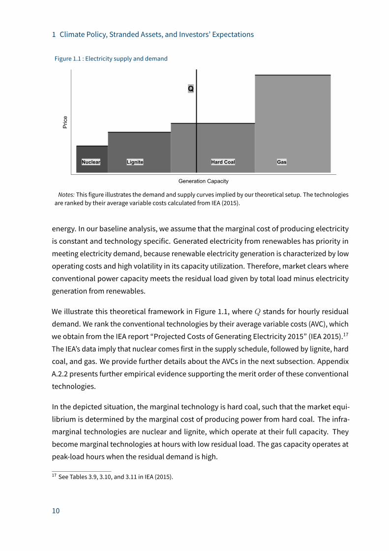
Notes: This figure illustrates the demand and supply curves implied by our theoretical setup. The technologiesare ranked by their average variable costs calculated from IEA (2015).
energy. In our baseline analysis, we assume that themarginal cost of producing electricity
is constant and technology specific. Generated electricity from renewables has priority in
meeting electricity demand, because renewable electricity generation is characterized by low
operating costs and high volatility in its capacity utilization. Therefore, market clears where
conventional power capacity meets the residual load given by total load minus electricity
generation from renewables.
We illustrate this theoretical framework in Figure 1.1, where Q stands for hourly residual
demand. We rank the conventional technologies by their average variable costs (AVC), which
we obtain from the IEA report “Projected Costs of Generating Electricity 2015” (IEA 2015).17
The IEA’s data imply that nuclear comes first in the supply schedule, followed by lignite, hard
coal, and gas. We provide further details about the AVCs in the next subsection. Appendix
A.2.2 presents further empirical evidence supporting themerit order of these conventional
technologies.
In the depicted situation, the marginal technology is hard coal, such that the market equi-
librium is determined by the marginal cost of producing power from hard coal. The infra-
marginal technologies are nuclear and lignite, which operate at their full capacity. They
becomemarginal technologies at hours with low residual load. The gas capacity operates at
peak-load hours when the residual demand is high.
17 See Tables 3.9, 3.10, and 3.11 in IEA (2015).
10

1 Climate Policy, Stranded Assets, and Investors’ Expectations
1.3.2 Estimation of themerit order curve
In this section, we describe how we map our economic environment to data. We conduct
this analysis in two steps. First, we determine the ranking of conventional technologies in
the supply schedule as breifly explained in the previous subsection. Second, we estimate
technology specific supply curves by using data onmarket prices. Next, we explain each of
these steps in detail.
As we will illustrate later in this section, our policy scenarios mainly change the ranking of
some part of the lignite capacity in the supply schedule. Therefore, we need to be able to
identify which generation capacities are subject to our policy shocks. Unfortunately, we do
not have the required data to achieve this identification at the level of capacity unit or at the
plant level. However, our assumption of technology-specific constant marginal cost enables
this analysis in two ways. First, we can rank the conventional technologies by their AVCs from
the IEA data. Second, as the marginal cost is assumed to be constant for each technology,
which part of the lignite capacity is replaced by the shock is irrelevant. The AVCs based on
the IEA data are depicted in Figure 1.2.18 We impose the illustrated ranking of conventional
technologies throughout our analysis. However, we do not prefer to use the AVCs themselves
as an approximation for the merit order curve. The reason is that the AVCs are not completely
in line with the market outcomes within our theoretical framework, which we show in the
following.
Under an inelastic demand assumption, the functional relation between electricity prices and
residual load traces a supply curve.19 Figure 1.2 also presents the observed prices and the
average prices within each technological supply range.20 The average price where hard coal
is assumed to be the marginal technology is quite close to the AVC of hard coal. However,
there are considerable di�erences between the AVCs and the average prices in the case of
lignite and gas. Therefore, we conduct our analysis with the average prices bymaintaining
18 In calculating these average variable costs, we include the fuel, carbon, andoperational andmaintenance costsreported in IEA (2015). However, we set the carbon price to $10 per tonne of CO2 which is a rough approximationof the ETSprice in 2015, instead of a $30 per tonne of CO2 carbonprice assumedby IEA. The range of technologicalcapacities are given by their net installed generation capacities obtained from thewebsite of Fraunhofer Institutefor Solar Energy Systems (ISE). See https://www.energy-charts.de/index.htm.19 See, for example, Bessembinder and Lemmon (2002) and Cludius et al. (2014) for estimations of electricitysupply curve from data onmarket outcomes.20 We obtain the residual load and price data at hourly resolution from the Open Energy Modeling Initiative(OEMI 2019). The prices are the day-ahead prices in the European Energy Exchange (EEX) for the German powermarket. Appendix A.2.1 presents further details about this dataset.
11
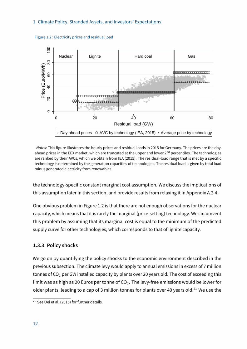
1 Climate Policy, Stranded Assets, and Investors’ Expectations
Figure 1.2 : Electricity prices and residual load
Nuclear Lignite Hard coal Gas
020
40
60
80
100
0 20 40 60 80
Day ahead prices AVC by technology (IEA, 2015) Average price by technology
Price
(E
uro
/MW
h)
Residual load (GW)
Notes: This figure illustrates the hourly prices and residual loads in 2015 for Germany. The prices are the day-ahead prices in the EEXmarket, which are truncated at the upper and lower 2nd percentiles. The technologiesare ranked by their AVCs, which we obtain from IEA (2015). The residual-load range that is met by a specifictechnology is determined by the generation capacities of technologies. The residual load is given by total loadminus generated electricity from renewables.
the technology-specific constant marginal cost assumption. We discuss the implications of
this assumption later in this section, and provide results from relaxing it in Appendix A.2.4.
One obvious problem in Figure 1.2 is that there are not enough observations for the nuclear
capacity, which means that it is rarely the marginal (price-setting) technology. We circumvent
this problem by assuming that its marginal cost is equal to the minimum of the predicted
supply curve for other technologies, which corresponds to that of lignite capacity.
1.3.3 Policy shocks
We go on by quantifying the policy shocks to the economic environment described in the
previous subsection. The climate levy would apply to annual emissions in excess of 7 million
tonnes of CO2 per GW installed capacity by plants over 20 years old. The cost of exceeding this
limit was as high as 20 Euros per tonne of CO2. The levy-free emissions would be lower for
older plants, leading to a cap of 3 million tonnes for plants over 40 years old.21 We use the
21 See Oei et al. (2015) for further details.
12
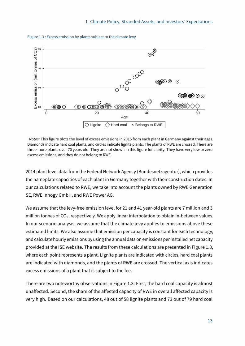
1 Climate Policy, Stranded Assets, and Investors’ Expectations
Figure 1.3 : Excess emission by plants subject to the climate levy0
12
3E
xcess e
mis
sio
n (
mil.
tonnes o
f C
O2)
0 20 40 60Age
Lignite Hard coal Belongs to RWE
Notes: This figure plots the level of excess emissions in 2015 from each plant in Germany against their ages.Diamonds indicate hard coal plants, and circles indicate lignite plants. The plants of RWE are crossed. There arethree more plants over 70 years old. They are not shown in this figure for clarity. They have very low or zeroexcess emissions, and they do not belong to RWE.
2014 plant level data from the Federal Network Agency (Bundesnetzagentur), which provides
the nameplate capacities of each plant in Germany together with their construction dates. In
our calculations related to RWE, we take into account the plants owned by RWE Generation
SE, RWE Innogy GmbH, and RWE Power AG.
We assume that the levy-free emission level for 21 and 41 year-old plants are 7 million and 3
million tonnes of CO2, respectively. We apply linear interpolation to obtain in-between values.
In our scenario analysis, we assume that the climate levy applies to emissions above these
estimated limits. We also assume that emission per capacity is constant for each technology,
andcalculatehourly emissionsbyusing theannual dataonemissionsper installednet capacity
provided at the ISE website. The results from these calculations are presented in Figure 1.3,
where each point represents a plant. Lignite plants are indicated with circles, hard coal plants
are indicated with diamonds, and the plants of RWE are crossed. The vertical axis indicates
excess emissions of a plant that is subject to the fee.
There are two noteworthy observations in Figure 1.3: First, the hard coal capacity is almost
una�ected. Second, the share of the a�ected capacity of RWE in overall a�ected capacity is
very high. Based on our calculations, 48 out of 58 lignite plants and 73 out of 79 hard coal
13
1 Climate Policy, Stranded Assets, and Investors’ Expectations
plants were over 20-years old by 2017. However, the policy is hardly binding for the hard coal
capacity as the average emissions from hard coal plants per GW-installed capacity were 3.4
million tonnes of CO2 in 2015. According to our calculations, the levy would be binding for
less than 4% of the hard coal capacity. Therefore, we ignore this point in our analysis. On
the other hand, the average emissions from lignite plants per GW installed capacity were 7.5
million tonnes of CO2. As a result, 29% of the lignite capacity would be subject to the climate
levy. Taking into account the average emissions per MWh of generation from lignite plants,
the marginal cost of a�ected lignite plants would increase by 28 Euros/MWh.22 This fee would
apply to 41% of RWE’s lignite capacity.
Themerit order e�ect of the climate levy is indirect through the resulting change in prices. On
the other hand, the security reserve proposal implies a direct change in the merit order. This
policy scenario phases out 2.7 GW lignite capacity andmoves it into a security reserve. In our
analysis, we ignore the latter implication and simply remove this capacity from the supply
schedule.23
1.3.4 Merit order e�ects
Next, we explain howour policy shocks a�ect the estimated supply curve. Figure 1.4 illustrates
the implications of our policy scenarios on the supply curve. In this figure, the capacities
that are a�ected by the policies and the generation capacity by technology are based on our
dataset. On the other hand, we set the cost levels in order to clarify the exposition. However,
the illustration preserves all the qualitative implications of our calculations. The average
residual demand for conventional power capacity in 2015 is indicated with Q. The figure
shows that, hard coal is the marginal technology at the average demand. This is in line with
the higher variability of generation from hard coal plants in Germany. We support this result
with further empirical evidence in Appendix A.2.2.24
The climate levy scenario leads to a drastic change in the merit order curve as illustrated in
the first panel of Figure 1.4. A considerable hard coal capacity replaces the a�ected lignite
capacity, which leads to a higher average cost ofmeeting the average load. The a�ected lignite
22 We obtain emission and generation data for lignite plants from the ISE charts, and calculate average emissionsper MWh of generation.23 See Table A.2 in Appendix A.2.3 for the list of units to be transferred into the security reserve.24 Also see the charts presented on the website of ISE for the variability of generation (https://www.energy-charts.de/index.htm).
14
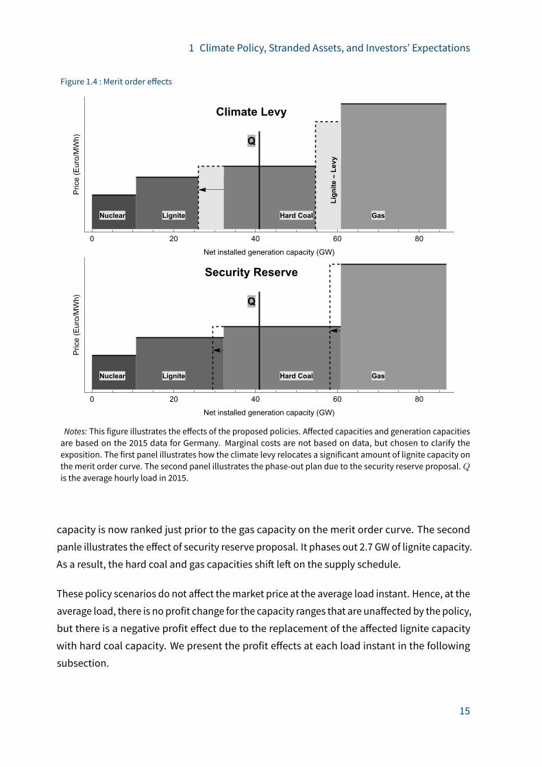
1 Climate Policy, Stranded Assets, and Investors’ Expectations
Figure 1.4 : Merit order e�ects
Nuclear Lignite Hard Coal Gas
Lignite-Levy
Q
Climate Levy
0 20 40 60 80
Net installed generation capacity (GW)
Price(Euro/MWh)
Nuclear Lignite Hard Coal Gas
Q
Security Reserve
0 20 40 60 80
Net installed generation capacity (GW)
Price(Euro/MWh)
Notes: This figure illustrates the e�ects of the proposed policies. A�ected capacities and generation capacitiesare based on the 2015 data for Germany. Marginal costs are not based on data, but chosen to clarify theexposition. The first panel illustrates how the climate levy relocates a significant amount of lignite capacity onthe merit order curve. The second panel illustrates the phase-out plan due to the security reserve proposal.Qis the average hourly load in 2015.
capacity is now ranked just prior to the gas capacity on the merit order curve. The second
panle illustrates the e�ect of security reserve proposal. It phases out 2.7 GW of lignite capacity.
As a result, the hard coal and gas capacities shi� le� on the supply schedule.
These policy scenarios do not a�ect themarket price at the average load instant. Hence, at the
average load, there is no profit change for the capacity ranges that are una�ected by the policy,
but there is a negative profit e�ect due to the replacement of the a�ected lignite capacity
with hard coal capacity. We present the profit e�ects at each load instant in the following
subsection.
15
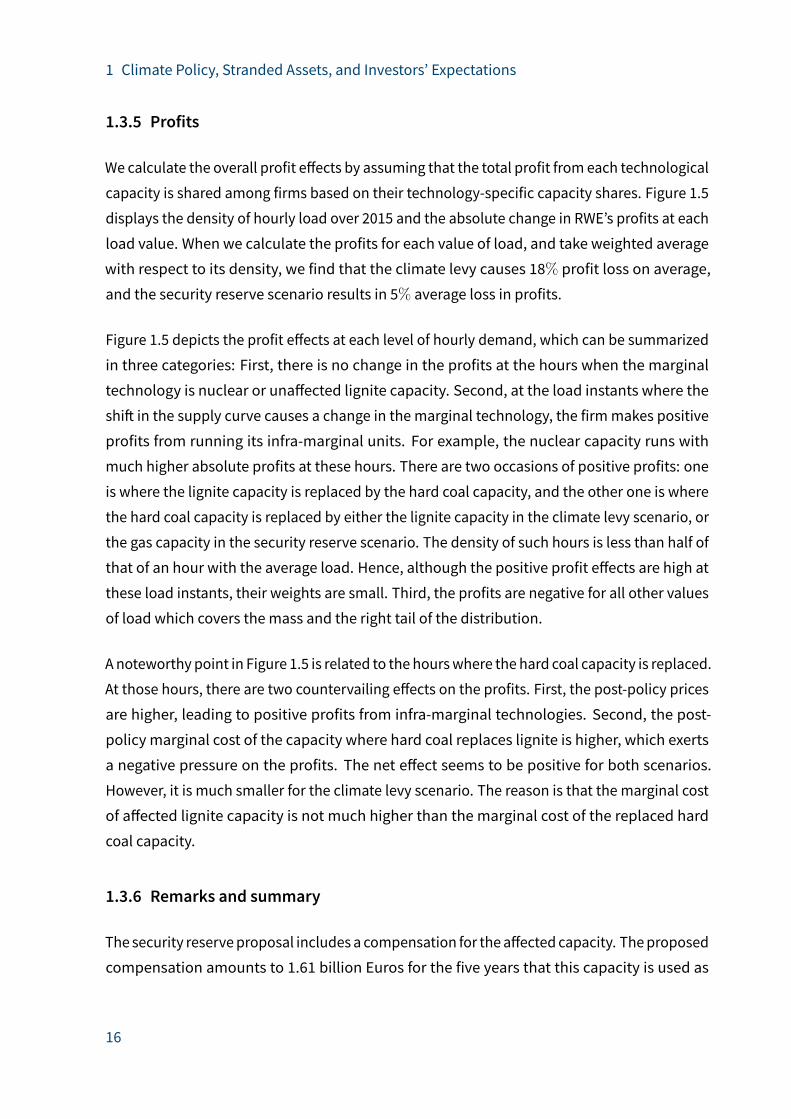
1 Climate Policy, Stranded Assets, and Investors’ Expectations
1.3.5 Profits
We calculate the overall profit e�ects by assuming that the total profit from each technological
capacity is shared among firms based on their technology-specific capacity shares. Figure 1.5
displays the density of hourly load over 2015 and the absolute change in RWE’s profits at each
load value. When we calculate the profits for each value of load, and take weighted average
with respect to its density, we find that the climate levy causes 18% profit loss on average,
and the security reserve scenario results in 5% average loss in profits.
Figure 1.5 depicts the profit e�ects at each level of hourly demand, which can be summarized
in three categories: First, there is no change in the profits at the hours when the marginal
technology is nuclear or una�ected lignite capacity. Second, at the load instants where the
shi� in the supply curve causes a change in the marginal technology, the firmmakes positive
profits from running its infra-marginal units. For example, the nuclear capacity runs with
much higher absolute profits at these hours. There are two occasions of positive profits: one
is where the lignite capacity is replaced by the hard coal capacity, and the other one is where
the hard coal capacity is replaced by either the lignite capacity in the climate levy scenario, or
the gas capacity in the security reserve scenario. The density of such hours is less than half of
that of an hour with the average load. Hence, although the positive profit e�ects are high at
these load instants, their weights are small. Third, the profits are negative for all other values
of load which covers the mass and the right tail of the distribution.
A noteworthy point in Figure 1.5 is related to the hourswhere the hard coal capacity is replaced.
At those hours, there are two countervailing e�ects on the profits. First, the post-policy prices
are higher, leading to positive profits from infra-marginal technologies. Second, the post-
policy marginal cost of the capacity where hard coal replaces lignite is higher, which exerts
a negative pressure on the profits. The net e�ect seems to be positive for both scenarios.
However, it is much smaller for the climate levy scenario. The reason is that the marginal cost
of a�ected lignite capacity is not much higher than the marginal cost of the replaced hard
coal capacity.
1.3.6 Remarks and summary
The security reserveproposal includes a compensation for thea�ected capacity. Theproposed
compensation amounts to 1.61 billion Euros for the five years that this capacity is used as
16
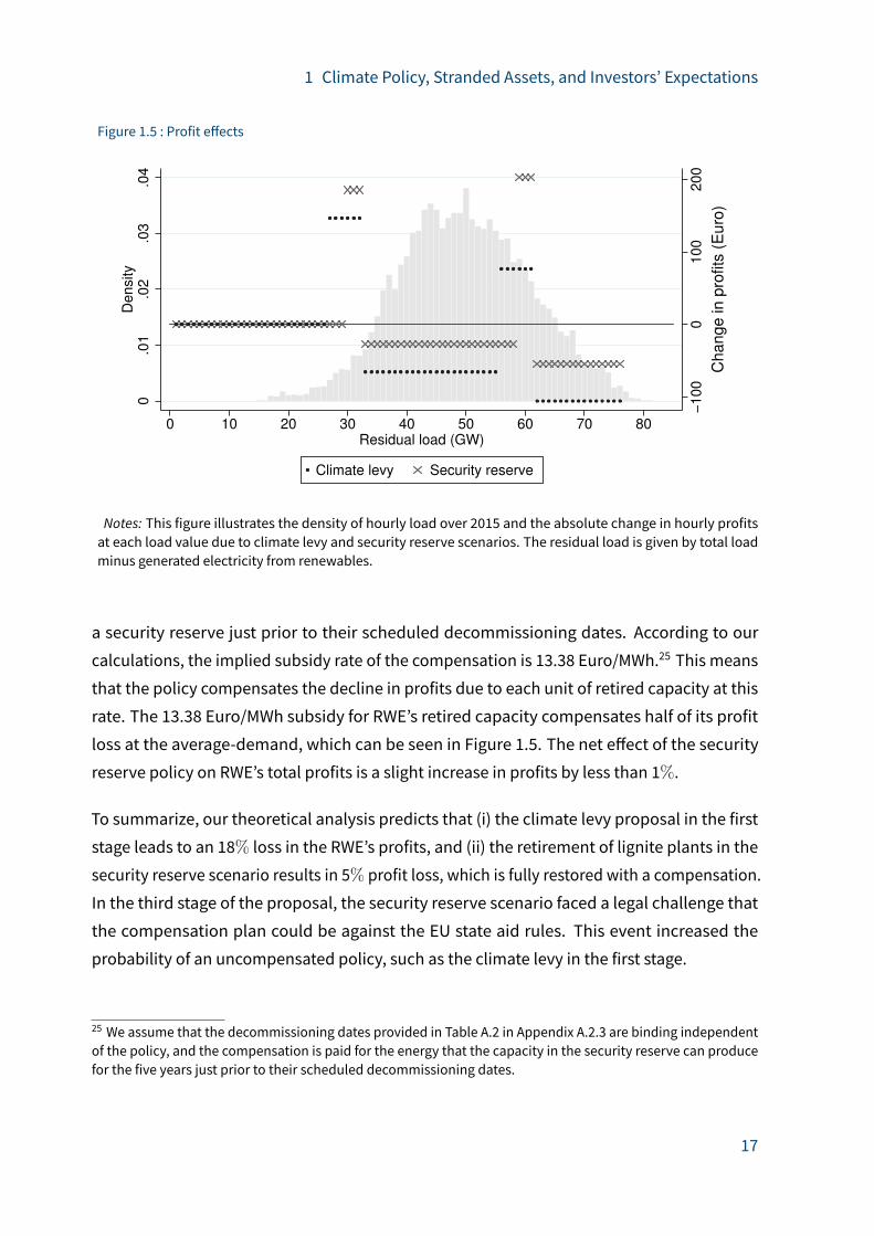
1 Climate Policy, Stranded Assets, and Investors’ Expectations
Figure 1.5 : Profit e�ects
−100
0100
200
0.0
1.0
2.0
3.0
4D
ensity
0 10 20 30 40 50 60 70 80Residual load (GW)
Climate levy Security reserve
Ch
an
ge
in
pro
fits
(E
uro
)
Notes: This figure illustrates the density of hourly load over 2015 and the absolute change in hourly profitsat each load value due to climate levy and security reserve scenarios. The residual load is given by total loadminus generated electricity from renewables.
a security reserve just prior to their scheduled decommissioning dates. According to our
calculations, the implied subsidy rate of the compensation is 13.38 Euro/MWh.25 This means
that the policy compensates the decline in profits due to each unit of retired capacity at this
rate. The 13.38 Euro/MWh subsidy for RWE’s retired capacity compensates half of its profit
loss at the average-demand, which can be seen in Figure 1.5. The net e�ect of the security
reserve policy on RWE’s total profits is a slight increase in profits by less than 1%.
To summarize, our theoretical analysis predicts that (i) the climate levy proposal in the first
stage leads to an 18% loss in the RWE’s profits, and (ii) the retirement of lignite plants in the
security reserve scenario results in 5% profit loss, which is fully restored with a compensation.
In the third stage of the proposal, the security reserve scenario faced a legal challenge that
the compensation plan could be against the EU state aid rules. This event increased the
probability of an uncompensated policy, such as the climate levy in the first stage.
25 We assume that the decommissioning dates provided in Table A.2 in Appendix A.2.3 are binding independentof the policy, and the compensation is paid for the energy that the capacity in the security reserve can producefor the five years just prior to their scheduled decommissioning dates.
17

1 Climate Policy, Stranded Assets, and Investors’ Expectations
In our analysis, we assume constant marginal cost per technology, and use the average prices
to approximate themerit order curve. An alternativeway is to allow for non-constantmarginal
costs by fitting technology-specific lines to the market data. We prefer the former method for
three reasons. First, it is much easier to illustrate the e�ect of these policy scenarios on the
supply schedule, which is the main goal of the current section. Second, each capacity unit
of lignite would have di�erent marginal cost under non-constant marginal cost assumption,
whereas we do not have data to identify the lignite units a�ected by the climate levy. This
point is not important under a constant marginal cost assumption. Third, the estimations of a
linear supply curve su�ers from simultaneity. As a result, estimated slopes based onmarket
data can be biased. Proper estimation of the supply curve is beyond the scope of our paper.
With a positively-sloped supply curve, however, the policy shocks lead to an increase in prices
at each point that the supply curve shi�s to le�. An increase in equilibrium prices a�ects
profits positively, in particular for infra-marginal nuclear and lignite capacities. Therefore,
relaxing the constantmarginal cost per technology assumptionmight yield lower profit e�ects
in absolute terms. We illustrate this e�ect in Appendix A.2.4 based on a naive supply curve
estimation.
1.4 Potential reactions and investors’ priors
Wewill draw conclusions about investors’ initial beliefs from their reactions to the di�erent
stages of the policy development. Table 1.2 outlines plausible belief updating scenarios.
Scenario 0 is no reaction: here, investors simply do not care about stranded asset risk and do
not react to any policy proposals or related news. In Scenario 1, the investors’ prior is that
unburnable carbon is of no concern. However, they do care about stranded asset risk induced
by specific policies, and react to such news. They are positively surprised by the compensation
mechanism and negatively by its challenge. In Scenario 2, investors have already priced in
stranded asset risk due to unburnable carbon: for example, they are aware of a nationwide
or worldwide emission reduction target and have already considered this overall target in
their firm valuation. Therefore, a policy introduced to achieve the target does not impact their
valuation of the a�ected firms. However, the compensation mechanism is unexpected for
these investors and they value it positively.26 When the compensation is challenged, they
26 Note that in this case, we would not expect a positive reaction for E.ON: only RWE receives compensationpayments, and investors are not concerned about introduction of the uncompensated policy in this scenario, asthey have already priced in general unburnable carbon risk.
18
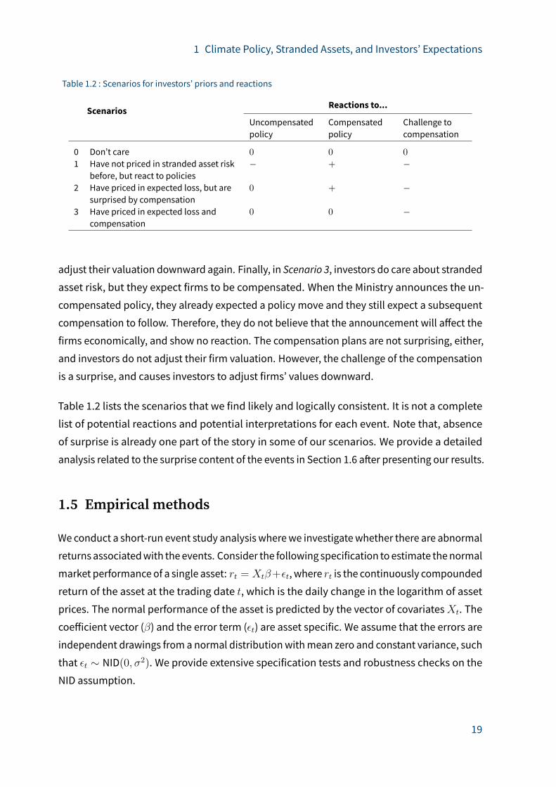
1 Climate Policy, Stranded Assets, and Investors’ Expectations
Table 1.2 : Scenarios for investors’ priors and reactions
ScenariosReactions to...
Uncompensatedpolicy
Compensatedpolicy
Challenge tocompensation
0 Don’t care 0 0 0
1 Have not priced in stranded asset riskbefore, but react to policies
− + −
2 Have priced in expected loss, but aresurprised by compensation
0 + −
3 Have priced in expected loss andcompensation
0 0 −
adjust their valuation downward again. Finally, in Scenario 3, investors do care about stranded
asset risk, but they expect firms to be compensated. When the Ministry announces the un-
compensated policy, they already expected a policy move and they still expect a subsequent
compensation to follow. Therefore, they do not believe that the announcement will a�ect the
firms economically, and show no reaction. The compensation plans are not surprising, either,
and investors do not adjust their firm valuation. However, the challenge of the compensation
is a surprise, and causes investors to adjust firms’ values downward.
Table 1.2 lists the scenarios that we find likely and logically consistent. It is not a complete
list of potential reactions and potential interpretations for each event. Note that, absence
of surprise is already one part of the story in some of our scenarios. We provide a detailed
analysis related to the surprise content of the events in Section 1.6 a�er presenting our results.
1.5 Empirical methods
We conduct a short-run event study analysis wherewe investigatewhether there are abnormal
returns associatedwith theevents. Consider the following specification toestimate thenormal
market performance of a single asset: rt = Xtβ+εt, where rt is the continuously compounded
return of the asset at the trading date t, which is the daily change in the logarithm of asset
prices. The normal performance of the asset is predicted by the vector of covariatesXt. The
coe�icient vector (β) and the error term (εt) are asset specific. We assume that the errors are
independent drawings from a normal distributionwithmean zero and constant variance, such
that εt ∼ NID(0, σ2). We provide extensive specification tests and robustness checks on the
NID assumption.
19
1 Climate Policy, Stranded Assets, and Investors’ Expectations
Event study approach is based on comparing realized returns on the event date with normal
returns. The normal return, which is an estimate of E[rt|Xt], is the predicted return given
by rt = Xtβ. We define the relative time index τ = t − T to measure the distance to
the event date T in terms of trading days. Then, the abnormal returns (AR) are given by
γT+τ = rT+τ − E[rT+τ |XT+τ ], and their estimates are the prediction errors, given by γT+τ =
rT+τ − rT+τ .
The null hypothesis that the event does not have an e�ect over the eventwindow is formulated
asH0:∑τ=h
τ=−h γT+τ = 0, where h is the half-width of the event window. Hence, the event
window spans the L = 2h+ 1 trading days from t = T − h to t = T + h. The sum over the
abnormal returns gives the cumulative abnormal return (CAR).
In order to apply the classical t-test, the variance of the CAR can be calculated as var(CAR) =
ι′V ι, where V is the L× L covariance matrix of abnormal returns and ι is an L× 1 vector of
ones. The variance of prediction errors has two components: sampling uncertainity in the
estimation of the model parameters and the error uncertainty. If the estimation sample is
su�iciently large, one can ignore the samplinguncertainty. Although the samplinguncertainity
in our application is small and does not a�ect any of our results, we do not ignore it. Sampling
uncertainty causes serial correlation among abnormal returns. Hence, V has non-zero o�-
diagonal elements. Its influence is typically very small in short-run event studies, which is
the case in our application too. In all our estimations, taking the correlation structure into
account does not lead to any visible di�erences. When the o�-diagonal elements are taken as
zero, var(CAR) =∑τ=h
τ=−h var(γT+τ ), where var(γT+τ ) is given by var(rT+τ ) + σ2. The first
term is due to sampling uncertainity, and the second term is the error variance.
To interpret the AR as the event e�ect, the required assumption is that the model is correctly
specified such that the predicted returns for the event window are the counterfactual returns
to the asset in the absence of the event. The choice of the covariate set is generally motivated
by well-known statistical and theoretical models of asset returns. We provide an extensive
robustness analysis with respect to this choice. In our baseline estimations, we simply use a
constant and returns to a market performance index (the so-called market model), which is
generally considered su�icient for short-run event studies (Campbell et al. 1997).
Valid estimation requires that the normal market performance is uncorrelated with the event-
induced abnormal returns. To control for potential feedback from the event to the normal
20
1 Climate Policy, Stranded Assets, and Investors’ Expectations
market performance, the common approach is to exclude the event window observations in
the estimation of expected returns. Given that abnormal returns are simply the prediction
errors, the natural choice for the estimation window is to use the observations prior to the
event window, potentially leaving a gap between the end of the estimation sample and the
beginning of the event window, which we call the “pseudo window”. In the absence of any
other event, the pseudo-window abnormal returns are expected to be insignificant. We
conduct performance tests for the predictive power of our model by calculatingL-days CARs
for each date in the pseudo window as if an event has occurred on that date.
Themost important threat to identification of the event e�ect is the presence of other contem-
poraneous shocks in the event window. There are several ways to control for such potential
biases. First, when there is a limited number of assets or announcements, it is feasible to
review the news around the event dates. We undertake this approach by using a news search
engine and we identify a small number of such potential confounding events, which will be
discussed in Section 1.7.2. Second, the event window should be kept reasonably small to
rule out other asset-specific events around the event window. Third, the market model can
capture the average e�ect of market-wide shocks via themarket price index. However, the
market price index is not a proper counterfactual control unit because the event-a�ected units
might participate in this portfolio, leaving the price index endogenous to the event shock. Also,
the weights of the market index are not intended to produce a control unit for the a�ected
company, but to reflect the average market conditions. In order to take care of this concern,
we apply a synthetic control approachwhich allows choosing assets to create a counterfactual
portfolio and estimating their weights.27 We provide a detailed description of this approach in
Appendix A.4.
To control for industry-wide shocks, we use EnBW as the control unit, a company in the same
industry but without any relevant lignite asset. Therefore, a priori, we do not expect the
series of events subject to our analysis to have any e�ect on EnBW. This gives a di�erence-in-
di�erences estimate of the abnormal returns by removing biases from industry-wide shocks
to returns to asset i.28 We provide a technical description of this approach in Appendix A.4.
27 See Abadie and Gardeazabal (2003) for the synthetic control estimation. See, for example, Guidolin andLa Ferrara (2007) for an application of synthetic control estimation in an event study analysis. An alternativeapproach might be to use a di�erent market index. This approach is less preferable, since our goal is to capturethe common shocks in the market that are most relevant for the subject firms.28 In terms of the synthetic control approach, this can be considered as assigning a weight of 1 to EnBW and 0 toall other assets in the donor pool.
21
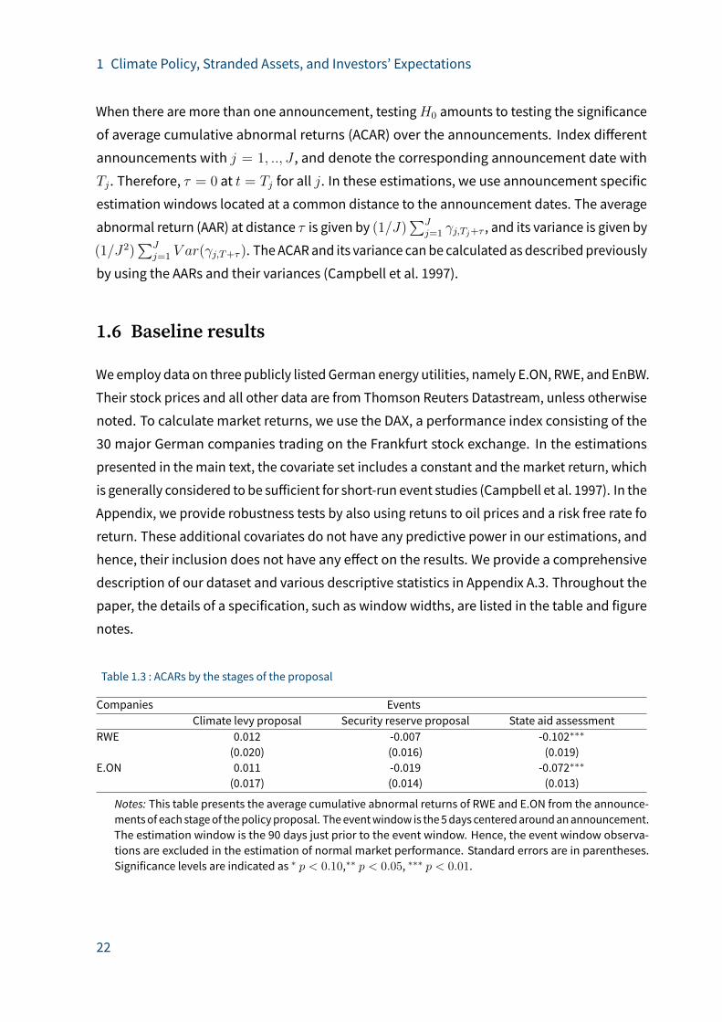
1 Climate Policy, Stranded Assets, and Investors’ Expectations
When there are more than one announcement, testingH0 amounts to testing the significance
of average cumulative abnormal returns (ACAR) over the announcements. Index di�erent
announcements with j = 1, .., J , and denote the corresponding announcement date with
Tj . Therefore, τ = 0 at t = Tj for all j. In these estimations, we use announcement specific
estimation windows located at a common distance to the announcement dates. The average
abnormal return (AAR) at distance τ is given by (1/J)∑J
j=1 γj,Tj+τ , and its variance is given by
(1/J2)∑J
j=1 V ar(γj,T+τ ). The ACARand its variance canbe calculated as describedpreviously
by using the AARs and their variances (Campbell et al. 1997).
1.6 Baseline results
Weemploy data on three publicly listedGerman energy utilities, namely E.ON, RWE, and EnBW.
Their stock prices and all other data are from Thomson Reuters Datastream, unless otherwise
noted. To calculate market returns, we use the DAX, a performance index consisting of the
30 major German companies trading on the Frankfurt stock exchange. In the estimations
presented in themain text, the covariate set includes a constant and themarket return, which
is generally considered to be su�icient for short-run event studies (Campbell et al. 1997). In the
Appendix, we provide robustness tests by also using retuns to oil prices and a risk free rate fo
return. These additional covariates do not have any predictive power in our estimations, and
hence, their inclusion does not have any e�ect on the results. We provide a comprehensive
description of our dataset and various descriptive statistics in Appendix A.3. Throughout the
paper, the details of a specification, such as windowwidths, are listed in the table and figure
notes.
Table 1.3 : ACARs by the stages of the proposal
Companies EventsClimate levy proposal Security reserve proposal State aid assessment
RWE 0.012 -0.007 -0.102∗∗∗
(0.020) (0.016) (0.019)E.ON 0.011 -0.019 -0.072∗∗∗
(0.017) (0.014) (0.013)
Notes: This table presents the average cumulative abnormal returns of RWE and E.ON from the announce-mentsof each stageof thepolicyproposal. Theeventwindow is the5days centeredaroundanannouncement.The estimation window is the 90 days just prior to the event window. Hence, the event window observa-tions are excluded in the estimation of normal market performance. Standard errors are in parentheses.Significance levels are indicated as ∗ p < 0.10,∗∗ p < 0.05, ∗∗∗ p < 0.01.
22
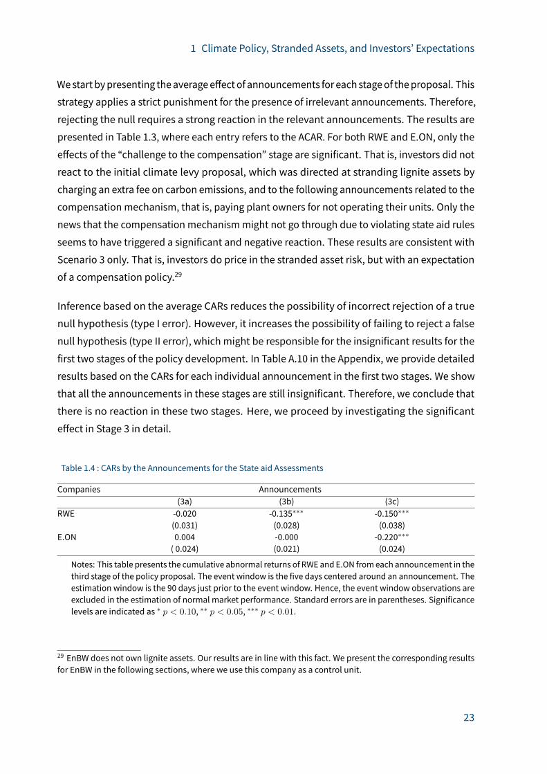
1 Climate Policy, Stranded Assets, and Investors’ Expectations
Westart bypresenting theaveragee�ectof announcements for each stageof theproposal. This
strategy applies a strict punishment for the presence of irrelevant announcements. Therefore,
rejecting the null requires a strong reaction in the relevant announcements. The results are
presented in Table 1.3, where each entry refers to the ACAR. For both RWE and E.ON, only the
e�ects of the “challenge to the compensation” stage are significant. That is, investors did not
react to the initial climate levy proposal, which was directed at stranding lignite assets by
charging an extra fee on carbon emissions, and to the following announcements related to the
compensation mechanism, that is, paying plant owners for not operating their units. Only the
news that the compensation mechanismmight not go through due to violating state aid rules
seems to have triggered a significant and negative reaction. These results are consistent with
Scenario 3 only. That is, investors do price in the stranded asset risk, but with an expectation
of a compensation policy.29
Inference based on the average CARs reduces the possibility of incorrect rejection of a true
null hypothesis (type I error). However, it increases the possibility of failing to reject a false
null hypothesis (type II error), which might be responsible for the insignificant results for the
first two stages of the policy development. In Table A.10 in the Appendix, we provide detailed
results based on the CARs for each individual announcement in the first two stages. We show
that all the announcements in these stages are still insignificant. Therefore, we conclude that
there is no reaction in these two stages. Here, we proceed by investigating the significant
e�ect in Stage 3 in detail.
Table 1.4 : CARs by the Announcements for the State aid Assessments
Companies Announcements(3a) (3b) (3c)
RWE -0.020 -0.135∗∗∗ -0.150∗∗∗
(0.031) (0.028) (0.038)E.ON 0.004 -0.000 -0.220∗∗∗
( 0.024) (0.021) (0.024)
Notes: This table presents the cumulative abnormal returns of RWE and E.ON fromeach announcement in thethird stage of the policy proposal. The event window is the five days centered around an announcement. Theestimation window is the 90 days just prior to the event window. Hence, the event window observations areexcluded in the estimation of normal market performance. Standard errors are in parentheses. Significancelevels are indicated as ∗ p < 0.10, ∗∗ p < 0.05, ∗∗∗ p < 0.01.
29 EnBW does not own lignite assets. Our results are in line with this fact. We present the corresponding resultsfor EnBW in the following sections, where we use this company as a control unit.
23
1 Climate Policy, Stranded Assets, and Investors’ Expectations
In Table 1.4, we present the test results based on individual CARs due to the announcements
in Stage 3. The results indicate that the ACARs in stage 3, presented in Table 1.3, are mainly
driven by the CARs during announcements (3b) and (3c): when themedia reported on the state
aid assessment by Parliament’s academic service, and when the EU Commission announced
opening the state aid procedure, respectively. Event (3a), the date at which the academic
service presented its report to Parliament, seems to have no significant e�ect on either firm.
The insignificant CAR due to this event is in line with our conjecture that this document was
not publicly available on that date. Only on the publication dates of the media reports of the
assessment do we observe a significant reaction.30 This pattern is in line with the assumption
that investors do not have access to insider information and price in only new information
made public via media reports.
The estimated average e�ect of the announcements related to state aid assessments on RWE
is larger, as also illustrated previously in Table 1.3. This result is in line with the fact that RWE
is more lignite-intensive (see Section 2). However, in the next section, we show that the ARs of
RWE due to event (3b) is partially driven by a strong negative earnings surprise, while E.ON is
experiencing a small positive earnings surprise. As a result, the di�erence in the reactions is
smaller. Overall, we do not find a significant di�erence between the reactions across these
two firms.
The results presented above show that investors do care about stranded asset risk, but that
they also expect a compensation policy for their economic losses. More specifically, investors
in stock markets did not react to the announcement of the climate levy proposal, as they
expect that the firms involved would not be financially a�ected. The underlying reason is that,
as their reactions to stages 2 and3 reveals, they expected that the firmswouldbe compensated
for their losses.
It is important that such an interpretation would not be possible by interpreting the reactions
to individual events independently, as investors’ reactions to policy signals depend on their
prior expectations. This is the idea underlying our strategy of tracking investors’ reactions in
the course of the development of a policy proposal. The significant reaction in Stage 3 shows
that there is a surprise element in the third stage. In the absence of confounding events, we
can conclude that this surprise was due to the challenge to the compensation policy. In the
next section, we show that the results from the third stage are not driven by confounding
30 The first report on the assessment was published by Der Spiegel (event 3b).
24
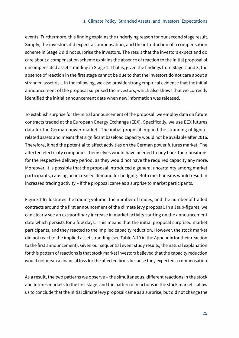
1 Climate Policy, Stranded Assets, and Investors’ Expectations
events. Furthermore, this finding explains the underlying reason for our second stage result.
Simply, the investors did expect a compensation, and the introduction of a compensation
scheme in Stage 2 did not surprise the investors. The result that the investors expect and do
care about a compensation scheme explains the absence of reaction to the initial proposal of
uncompensated asset stranding in Stage 1. That is, given the findings from Stage 2 and 3, the
absence of reaction in the first stage cannot be due to that the investors do not care about a
stranded asset risk. In the following, we also provide strong empirical evidence that the initial
announcement of the proposal surprised the investors, which also shows that we correctly
identified the initial announcement date when new information was released.
To establish surprise for the initial announcement of the proposal, we employ data on future
contracts traded at the European Energy Exchange (EEX). Specifically, we use EEX futures
data for the German power market. The initial proposal implied the stranding of lignite-
related assets andmeant that significant baseload capacity would not be available a�er 2016.
Therefore, it had the potential to a�ect activities on the German power futures market. The
a�ected electricity companies themselves would have needed to buy back their positions
for the respective delivery period, as they would not have the required capacity any more.
Moreover, it is possible that the proposal introduced a general uncertainty among market
participants, causing an increased demand for hedging. Both mechanisms would result in
increased trading activity – if the proposal came as a surprise to market participants.
Figure 1.6 illustrates the trading volume, the number of trades, and the number of traded
contracts around the first announcement of the climate levy proposal. In all sub-figures, we
can clearly see an extraordinary increase in market activity starting on the announcement
date which persists for a few days. This means that the initial proposal surprised market
participants, and they reacted to the implied capacity reduction. However, the stock market
did not react to the implied asset stranding (see Table A.10 in the Appendix for their reaction
to the first announcement). Given our sequential event study results, the natural explanation
for this pattern of reactions is that stockmarket investors believed that the capacity reduction
would not mean a financial loss for the a�ected firms because they expected a compensation.
As a result, the two patterns we observe – the simultaneous, di�erent reactions in the stock
and futures markets to the first stage, and the pattern of reactions in the stock market – allow
us to conclude that the initial climate levy proposal came as a surprise, but did not change the
25
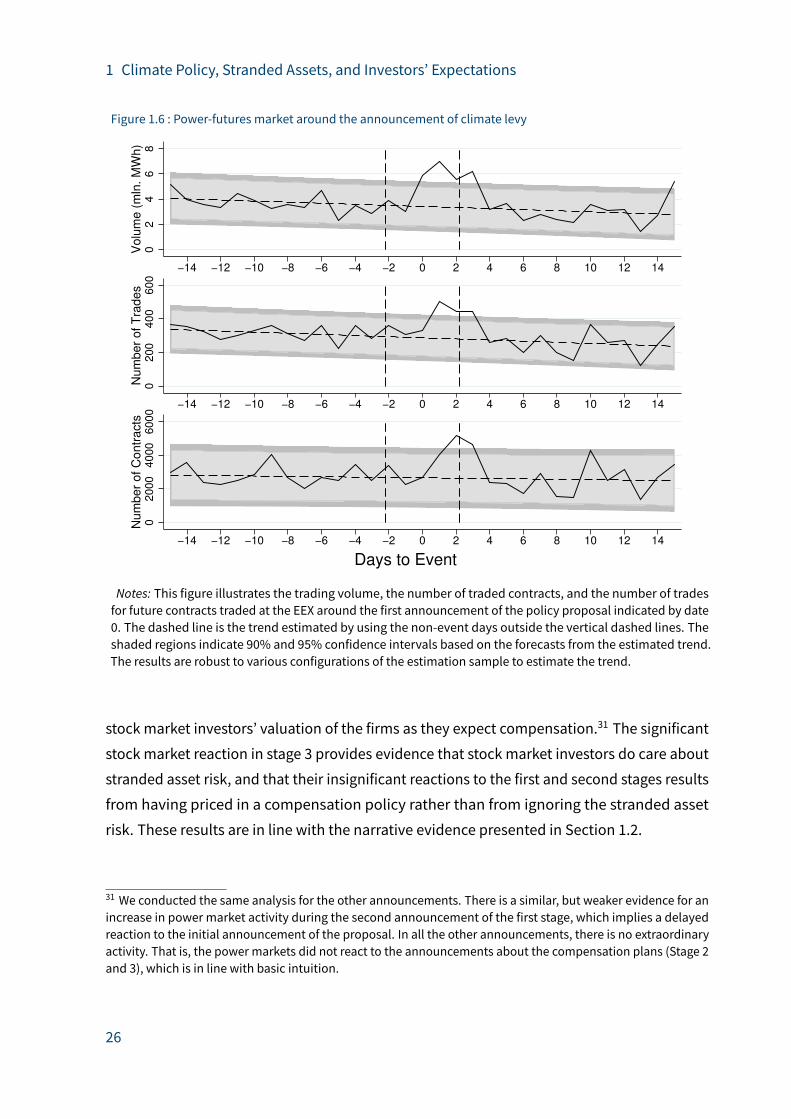
1 Climate Policy, Stranded Assets, and Investors’ Expectations
Figure 1.6 : Power-futures market around the announcement of climate levy
02
46
8V
olu
me (
mln
. M
Wh)
−14 −12 −10 −8 −6 −4 −2 0 2 4 6 8 10 12 14
02
00
40
06
00
Num
ber
of T
rades
−14 −12 −10 −8 −6 −4 −2 0 2 4 6 8 10 12 14
02
00
04
00
06
00
0N
um
ber
of C
ontr
acts
−14 −12 −10 −8 −6 −4 −2 0 2 4 6 8 10 12 14
Days to Event
Notes: This figure illustrates the trading volume, the number of traded contracts, and the number of tradesfor future contracts traded at the EEX around the first announcement of the policy proposal indicated by date0. The dashed line is the trend estimated by using the non-event days outside the vertical dashed lines. Theshaded regions indicate 90% and 95% confidence intervals based on the forecasts from the estimated trend.The results are robust to various configurations of the estimation sample to estimate the trend.
stock market investors’ valuation of the firms as they expect compensation.31 The significant
stock market reaction in stage 3 provides evidence that stock market investors do care about
stranded asset risk, and that their insignificant reactions to the first and second stages results
from having priced in a compensation policy rather than from ignoring the stranded asset
risk. These results are in line with the narrative evidence presented in Section 1.2.
31 We conducted the same analysis for the other announcements. There is a similar, but weaker evidence for anincrease in power market activity during the second announcement of the first stage, which implies a delayedreaction to the initial announcement of the proposal. In all the other announcements, there is no extraordinaryactivity. That is, the power markets did not react to the announcements about the compensation plans (Stage 2and 3), which is in line with basic intuition.
26

1 Climate Policy, Stranded Assets, and Investors’ Expectations
1.7 Robustness analysis
We present the results from alternative modeling choices in the Appendix. First, in Appendix
A.5, we show that our results are robust to using a three-day event window, and employing oil
prices and interest rates in the predictionmodel.32 Second, we provide extensive specification
tests and robustness checks on the assumed error distribution by using both resampling and
analytical techniques. These results are presented in Appendix A.6. In the rest of the paper, we
present robustness tests on two other dimensions. In Section 1.7.1, we focus on analyzing our
model’s performance in identifying the event e�ect. In Section 1.7.2, we investigate whether
there are confounding events around the announcement dates that might drive our baseline
results.
1.7.1 Placebo tests andmodel specification
We start by conducting placebo tests by assuming false event windows just prior to our events.
This analysis validates our model’s performance in predicting the counterfactual returns.
Second, we conduct synthetic control estimations to verify that our results are not driven by
the endogeneity issue due to the presence of E.ON’s and RWE’s assets in the DAX30 index.
The results from the placebo tests are presented in Figure 1.7. On each graph, the le� panel
separated by the dashed line is the pseudo-event window, and the right panel is the event
window. Each point on a graph refers to the CAR calculated from the abnormal returns on
the five days centered around that date.33 The estimated CARs for date zero (the event date)
correspond to the results presented in Table 1.4. The 90% and 95% confidence intervals for
the CARs are illustrated as forecast intervals to ease the readability.
Figure 1.7 shows that the model performs well in predicting the out-of-sample returns in
the pseudo window, thus increasing confidence in our model specification. Furthermore,
there seems to be no sign of other events in the pseudo windows that bias the estimated CAR
around the event day. For the significant events, theCARs are generally stable and insignificant
throughout the pseudo window and gradually become negative and significant in the event
windows. The gradual change in the CARs and the presence of significant CARs just before
the event window is not surprising as we use five-day rolling windows. For example, the
32 We have verified that our results are robust to using 45, 60, and 120 observations for the estimation sample.33 Corresponding estimated abnormal returns are provided in Figure A.13 in the Appendix.
27
1 Climate Policy, Stranded Assets, and Investors’ Expectations
Figure 1.7 : Impact of state aid assessments
−.2
−.1
0.1
−8 −6 −4 −2 0 2
RWE − Event (3a)
−.2
−.1
0.1
−8 −6 −4 −2 0 2
RWE − Event (3b)
−.2
−.1
0.1
−8 −6 −4 −2 0 2
RWE − Event (3c)−
.2−
.10
.1
−8 −6 −4 −2 0 2
E.ON − Event (3a)
−.2
−.1
0.1
−8 −6 −4 −2 0 2
E.ON − Event (3b)
−.2
−.1
0.1
−8 −6 −4 −2 0 2
E.ON − Event (3c)
5−
da
ys R
olli
ng
CA
Rs
Days to Event
Notes: This figure presents the CARs of E.ON and RWE from each announcement in the third stage of thepolicy proposal. The event window is the five days centered around an announcement (date 0) indicated withthe dashed lines. In the figure, the days prior to the event window are the lacebo announcement days. Theestimationwindow is the 90days just prior to the pseudowindow. Hence, the eventwindowandpseudowindowobservations are excluded in the estimation of normal market performance. The 90% and 95% confidenceintervals are indicated by shaded areas.
calculation of the five-day rolling CAR on date 3, which is in the pseudo window, employs
two abnormal returns from the event window. The observed pattern indicates that the event
e�ects seem to be well captured by the five-day event window.
To control for potential biases due to the endogeneity of the DAX30 index, we perform syn-
thetic control estimations. Here, we estimate a synthetic portfolio using DAX30 companies by
excluding RWE and E.ON. We base the matching procedure only on the asset returns of these
companies. The technical details are provided in Appendix A.4.1. The results are presented in
28

1 Climate Policy, Stranded Assets, and Investors’ Expectations
Figure 1.8 : Synthetic control estimations−
.3−
.2−
.10
.1
−8 −6 −4 −2 0 2
RWE − Event (3a)
−.3
−.2
−.1
0.1
−8 −6 −4 −2 0 2
RWE − Event (3b)
−.3
−.2
−.1
0.1
−8 −6 −4 −2 0 2
RWE − Event (3c)
−.3
−.2
−.1
0.1
−8 −6 −4 −2 0 2
E.ON − Event (3a)
−.3
−.2
−.1
0.1
−8 −6 −4 −2 0 2
E.ON − Event (3b)
−.3
−.2
−.1
0.1
−8 −6 −4 −2 0 2
E.ON − Event (3c)
5−
da
ys R
olli
ng
CA
Rs
Days to Event
Notes: This figure presents the synthetic control estimations of the CARs of E.ON and RWE from each an-nouncement in the third stage of the policy proposal. The event window is the five days centered around anannouncement (date 0) indicated with the dashed lines. The days prior to the event window are the placeboannouncement days. The estimation window is the 90 days just prior to the pseudo window. Hence, the eventwindow and pseudo window observations are excluded in the estimation of normal market performance. Thein-place placebo tests are illustrated with grey lines, and the grey areas are 90% and 95% confidence intervalsconstructed from the pre-treatment RMSE.
Figure 1.8.34 While the qualitative results remain the same, the estimated sizes of the CARs
are slightly larger. This indicates that the market price index might have been a�ected by the
events subject to our analysis and therefore absorbed some of the event e�ects. However,
the size of this bias is very small and negligible for all the events.
Figure 1.8 further illustrates some inputs to conduct the non-parametric inference strategy
suggested by Abadie et al. (2015) for synthetic control estimations. The so-called “in-place
placebo” estimations, which are estimations of the event e�ect on the units in the control34 See Figure A.15 in the Appendix for the corresponding abnormal returns.
29
1 Climate Policy, Stranded Assets, and Investors’ Expectations
group (donor pool), are illustrated with grey lines. The shaded areas are 90% and 95% predic-
tion intervals constructed from the pre-treatment root mean squared error (RMSE). It is seen
that the predicted CARs of untreated units are generally within the prediction intervals which
confirms the predictive power of the model.35 Second, the CARs for E.ON and RWE during
the event window are extraordinarily higher than the CARs of untreated units. These results
are in line with our baseline estimations. We present the non-parametric p-values based on
the in-place placebo tests in Table A.14 in the Appendix, which are in line with our baseline
estimations.
1.7.2 Confounding events
In this section, we control for the presence of confounding events around the announcement
dates that might partially or completely drive our baseline results. To detect confounding
events, we used a news search engine and conducted a careful review of the news published
around the announcement dates of events (3b) and (3c). The search methodology and a
summary of all the results are provided in Appendix A.7. Our search resulted in two news
items.
The first item is the nuclear provisioning assessment announcement and is potentially relevant
for both RWE and E.ON. On September 10, the first trading date in the event window of
announcement (3c), the media reported the results of a study commissioned by the Ministry
of Economy and Energy.36 This study concluded that the energy companies’ provisioning
for liabilities in connection with nuclear plant decommissioning and waste disposal was
insu�icient. Although this study did not imply direct political or financial consequences, one
could imagine that investors reacted to it.
The second item is earnings announcements. Both E.ON and RWE published their quarterly
earnings announcements just before announcement (3b) – on August 12 and August 13,
respectively. Since the announced earnings are company specific, this event has the potential
to induce the patterns in the estimated CARs for announcement (3b).
35 The reason underlying the higher dispersion in the in-place placebo CARs around event (3b) will be clarified inthe next subsection.36 See http://www.spiegel.de/wirtschaft/unternehmen/atomausstieg-fuer-den-atommuell-fehlen-30-milliarden-euro-a-1052869.html. For an English-language account of the study and its potentialimplications for the firms’ credit ratings, see https://www.moodys.com/research/Moodys-Nuclear-shutdown-costs-stress-German-power-generators--PR_335268.
30

1 Climate Policy, Stranded Assets, and Investors’ Expectations
Controlling for the nuclear provisioning assessment In order to control for the nuclear
provisioning assessment, we use EnBW, a company from the same industry but without rele-
vant lignite assets, as the single control unit. This strategy leads to a di�erence-in-di�erences
estimation of abnormal returns by removing the e�ects of common industry-wide shocks (see
Appendix A.4.2 for technical details). The nuclear provisioning assessment can be classified
as an industry-wide shock. First, the assessment does not target a specific company, but all
companies with nuclear power plants. Second, the problem of nuclear waste is relevant not
only for RWE and E.ON, but also for EnBW, which has substantial shares of nuclear energy
in its generation portfolio.37 On the other hand, the lignite policy proposal is irrelevant for
EnBW, since it does not hold any asset targeted by the proposal. Therefore, if the nuclear
provisioning assessment had any e�ect, it should be reflected in EnBW’s asset returns. By
using EnBW as a control unit, we can eliminate the influence of common systematic shocks in
a general manner.
Figure 1.9 : Pseudo tests on EnBW
−.2
−.1
0.1
−8 −6 −4 −2 0 2
Event (3a)
−.2
−.1
0.1
−8 −6 −4 −2 0 2
Event (3b)−
.2−
.10
.1
−8 −6 −4 −2 0 2
Event (3c)
5−
days R
olli
ng C
AR
s
Days to Event
Notes: This figure presents the CARs of EnBW from each announcement in the third stage of the policy proposal.The event window is the five days centered around an announcement (date 0) indicated with the dashed lines.The days prior to the event window are the placebo announcement days. The estimation window is the 90 daysjust prior to the pseudo window. Hence, the event window and pseudo window observations are excluded inthe estimation of normal market performance. The 90% and 95% confidence intervals are indicated by shadedareas.
This approach requires that (i) the events subject to our analysis had no impact on EnBW’s
asset returns, and (ii) any systematic di�erence between the a�ected units and EnBW can be
captured by the set of control variables. To assess the validity of EnBW as a control unit, we
37 According to the firms’ annual reports, 23% of EnBW’s installed capacity in 2015 was nuclear power plants,compared to 15% for RWE and 28% for E.ON.
31
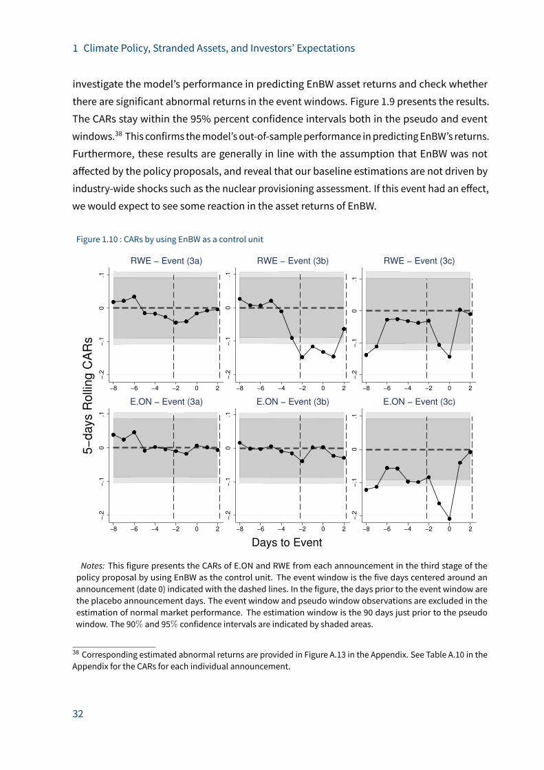
1 Climate Policy, Stranded Assets, and Investors’ Expectations
investigate the model’s performance in predicting EnBW asset returns and check whether
there are significant abnormal returns in the event windows. Figure 1.9 presents the results.
The CARs stay within the 95% percent confidence intervals both in the pseudo and event
windows.38 This confirms themodel’s out-of-sampleperformance inpredictingEnBW’s returns.
Furthermore, these results are generally in line with the assumption that EnBW was not
a�ected by the policy proposals, and reveal that our baseline estimations are not driven by
industry-wide shocks such as the nuclear provisioning assessment. If this event had an e�ect,
we would expect to see some reaction in the asset returns of EnBW.
Figure 1.10 : CARs by using EnBW as a control unit
−.2
−.1
0.1
−8 −6 −4 −2 0 2
RWE − Event (3a)
−.2
−.1
0.1
−8 −6 −4 −2 0 2
RWE − Event (3b)
−.2
−.1
0.1
−8 −6 −4 −2 0 2
RWE − Event (3c)
−.2
−.1
0.1
−8 −6 −4 −2 0 2
E.ON − Event (3a)
−.2
−.1
0.1
−8 −6 −4 −2 0 2
E.ON − Event (3b)
−.2
−.1
0.1
−8 −6 −4 −2 0 2
E.ON − Event (3c)
5−
days R
olli
ng C
AR
s
Days to Event
Notes: This figure presents the CARs of E.ON and RWE from each announcement in the third stage of thepolicy proposal by using EnBW as the control unit. The event window is the five days centered around anannouncement (date 0) indicated with the dashed lines. In the figure, the days prior to the event window arethe placebo announcement days. The event window and pseudo window observations are excluded in theestimation of normal market performance. The estimation window is the 90 days just prior to the pseudowindow. The 90% and 95% confidence intervals are indicated by shaded areas.
38 Corresponding estimated abnormal returns are provided in Figure A.13 in the Appendix. See Table A.10 in theAppendix for the CARs for each individual announcement.
32

1 Climate Policy, Stranded Assets, and Investors’ Expectations
The estimation results from using EnBW as the control unit are presented in Figure 1.10.39
Despite being slightly less precise, these estimations are generally in line with their baseline
counterparts in Figure 1.7. The size of the estimated CARs for the event windows is close to
those in our baseline estimations, indicating that our results are not driven by some industry-
level confounding event such as the report on nuclear waste liabilities (see Table A.16 in the
Appendix for details).
Controlling for earnings announcements The second news item in our search for con-
founding events is an earnings announcement (EA) just before announcement (3b). The
surprise content of announced earnings are company specific. Therefore, their influence on
the estimation results cannot be eliminated by using a control unit. Our strategy to control
for the earnings announcement is to correct the CARs on the date of announcement (3b) for
predicted abnormal returns due to the earnings surprise.
We proxy the expected earnings with the quarterly earnings forecasts reported by the In-
stitutional Brokers Estimate System (I/B/E/S), which is the mean of earnings forecasts by
many analysts for a large number of firms. Our measure of surprise is the di�erence between
announced earnings (AE) andmean forecasted earnings (MFE) normalized by the standard
deviation of the forecasts, namely, standardized unexpected earnings (SUE) provided by the
Thomson Reuters Database.
The technical details of estimating the marginal e�ect of SUE are provided in Appendix A.4.3.
We provide all the details from each step of these estimations in Appendix A.8. To summarize,
we start by estimating the five-day CARs for all the earnings announcements in our sample by
excluding the two earnings announcements by E.ON and RWE just before event (3b). Next, we
estimate the marginal e�ect of SUE on the predicted CARs. Finally, we extrapolate this result
to the excluded earnings announcements of RWE and E.ON around event (3b). Finally, we
adjust the CARs due to event (3b) with the predicted e�ect of the earnings announcements.
We repeat pseudo tests on event (3b) (see Figure 1.7) by taking the predicted e�ect of the
earnings announcement into account. The results are presented in Figure 1.11, where both
the rolling CARs and the prediction intervals are corrected for the size of and uncertainty
39 Other related results are presented in the Appendix: see Figure A.16 for the corresponding abnormal returns.The estimation tables by events and by announcements are provided in Tables A.15 and A.16, respectively.
33
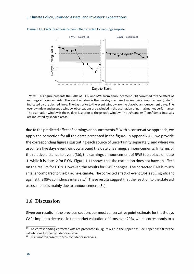
1 Climate Policy, Stranded Assets, and Investors’ Expectations
Figure 1.11 : CARs for announcement (3b) corrected for earnings surprise
−.2
−.1
0.1
−8 −7 −6 −5 −4 −3 −2 −1 0 1 2
RWE − Event (3b)
−.2
−.1
0.1
−8 −7 −6 −5 −4 −3 −2 −1 0 1 2
E.ON − Event (3b)
5−
da
ys R
olli
ng
CA
Rs
Days to Event
Notes: This figure presents the CARs of E.ON and RWE from announcement (3b) corrected for the e�ect ofearnings announcements. The event window is the five days centered around an announcement (date 0),indicated by the dashed lines. The days prior to the event window are the placebo announcement days. Theevent window and pseudo window observations are excluded in the estimation of normal market performance.The estimation window is the 90 days just prior to the pseudo window. The 90% and 95% confidence intervalsare indicated by shaded areas.
due to the predicted e�ect of earnings announcements.40 With a conservative approach, we
apply the correction for all the dates presented in the figure. In Appendix A.8, we provide
the corresponding figures illustrating each source of uncertainity separately, and where we
assume a five days event window around the date of earnings announcements. In terms of
the relative distance to event (3b), the earnings announcement of RWE took place on date
-1, while it is date -2 for E.ON. Figure 1.11 shows that the correction does not have an e�ect
on the results for E.ON. However, the results for RWE changes. The corrected CAR is much
smaller compared to the baseline estimate. The corrected e�ect of event (3b) is still significant
against the 95% confidence intervals.41 These results suggest that the reaction to the state aid
assessments is mainly due to announcement (3c).
1.8 Discussion
Given our results in the previous section, our most conservative point estimate for the 5-days
CARs implies a decrease in the market valuation of firms over 20%, which corresponds to a
40 The corresponding corrected ARs are presented in Figure A.17 in the Appendix. See Appendix A.8 for thecalculations for the confidence interval.41 This is not the case with 99% confidence intervals.
34

1 Climate Policy, Stranded Assets, and Investors’ Expectations
4% average abnormal return over the 5 days around the event. Given RWE’s considerable
market value (see Table A.3 in Appendix A.3), themonetary impact amounts to around 2 billion
Euros. These results show that the investors expect substantial costs from an uncompensated
policy, such as the climate levy scenario which becamemore likely a�er the compensation
for the security-reserve plan faced a legal challenge. This result is in line with our theoretical
predictions for RWE in Section 1.3, that the profit e�ect of the climate levy scenario can be as
high as 18%.
Note that our theoretical predictions are likely to be upper bounds, as allowing for non-
constant marginal costs generally reduces the negative profit e�ects. Therefore, our empirical
results imply a slightly highermarket reaction compared to the rangeof theoretical predictions
on the rate of change in RWE’s profits. The market value of a firm can be seen as a measure of
the capitalized risk-adjusted present value of future profit flows. Therefore, the di�erences
can be due to the uncertainty introduced by these announcements. Note that confirming
this di�erence statistically is not possible due to the level of uncertainty surrounding these
predictions.
1.9 Conclusion
We analyze the stock market e�ects of a German climate policy proposal aimed at stranding
fossil assets. We exploit the fact that the proposal underwent three stages. It started as a
“climate levy” increasing the CO2 price for power plants older than 20 years and was subse-
quently turned into a compensation mechanism paying individual lignite-fired power plants
for phasing out. In the third stage, the adoption of the compensation scheme was challenged
based on the possibility that it may violate EU state aid rules. We test the e�ects of news
about the di�erent stages of the policy proposal on the German utility companies. We find no
significant reactions to the first and second stages, but a significant and negative reaction to
the third stage for RWE and E.ON.
Our results suggest that compensation mechanisms are expected and thus priced in the
valuation of firms ex-ante. This finding implies that investors do care about stranded asset
risk, but because of the expectation of compensation, they do not believe that they will be
financially a�ected – neither by general unburnable carbon risk nor due to specific policy
proposals implying the stranding of assets. Only the challenge to the compensation changes
35
1 Climate Policy, Stranded Assets, and Investors’ Expectations
their beliefs. Our results imply that the e�ect of suchpolicy announcements canbe substantial.
Our most conservative estimates for 5-days CARs imply a loss over 20%.
Stranded asset risk is relevant for the energy sector and beyond. Most fossil energy assets are
long-lived; they usually require a large initial investment, but have relatively low operating
costs. S. J. Davis and Socolow (2014) show that expected future cumulative emissions from
the existing infrastructure of the global power sector have increased dramatically in the
last decades. Such long-term investments have the potential to “lock in” carbon-intensive
technologies for a long period of time (Erickson et al. 2015).42 Calculations by IEA (2013) and
Pfei�er et al. (2016) conclude that the “2 degree capital stock” will already be reached in 2017.
Investments in fossil capacities a�er 2017 are ine�icient: they lead to “both larger carbon lock-
ins and higher short-term emissions that need to be compensated by deeper emissions cuts
in the long run” (IPCC 2014a), increasing the cost of climate changemitigation. Moreover, in
order to achieve emission cuts in such a scenario, fossil assets need to be stranded. IEA (2013)
provides a conservative estimate that the energy industry faces sunk costs of $ 120 billion due
to fossil fuel plants being retired early, even if action to achieve the 2◦Cgoal had started in 2012.
For a scenario of delaying climate action until 2030 (and using a di�erentmethodology), IRENA
(2017a) estimates stranded assets of $ 1.9 trillion in electricity generation, and an additional
$ 7 trillion in upstream energy infrastructure (mostly oil production). This is approximately
equivalent to 3.5% of global income, and implies a risk not just for the obviously a�ected
energy industry facing sunk costs: international organizations, financial institutions and
regulators are increasingly concerned about the “transition risk” of climate policy, especially
about a sudden re-pricing of assets.43
A sudden devaluation of energy companies will occur only if expectations were not adjusted
in accordance with the risk of asset stranding. Sudden changes in the stringency of carbon
policies, or expectations in the presence of tipping points can lead to abrupt repricing of fossil
fuel assets. Given energy companies’ size and interrelation with the rest of the economy,
policymakers may regard energy companies as “too big to fail.” For this and other political
economy reasons,44 policymakers may opt for compensation policies, and investors may
42 Also see Unruh and Carrillo-Hermosilla (2006), Seto et al. (2016), and Unruh (2000, 2002).43 Cf., e.g., European Systemic Risk Board (2016a), Caldecott et al. (2016), IRENA (2017b), Batten et al. (2016),Banque de France (2015), and Baron and Fischer (2015). Also, see Johnson et al. (2015), Rozenberg et al. (2015),and Iyer et al. (2015) for the estimates of long-term energy- and economic-costs of the 2◦C goal.44 See Jenkins (2014), Manley et al. (2016), Healy and Barry (2017), and Caldecott et al. (2017) for an overview ofpolitical economy constraints on climate policy.
36

1 Climate Policy, Stranded Assets, and Investors’ Expectations
expect them to do so. Compensations, then, are almost a self-fulfilling prophecy: if they are
expected, they will be necessary in order to avoid larger shocks.45 Therefore, understanding
the interaction between policy making and investors’ expectations is essential for the design
of climate policies. Our results suggest that early and credible commitment to climate policies
and whether they involve compensation payments or not is crucial. Such clear signals to
financial markets can avoid a disruptive and unorderly energy transition andmacro shocks,
while directing capital towards climate-friendly technologies. We believe that further research
in similar contexts can help to generalize these results, or to identify the important factors in
the formation of expectations regarding climate related risks.
45 Batten et al. (2016) use a similar argument referring to the potential time inconsistency of government policiesin the context of stranded assets. They do not consider compensations, however, but only distinguish between a“low carbon equilibrium” and a “high carbon equilibrium.”
37

2 Institutional Investors, Climate Policy Risk, andDirected Innovation
2.1 Introduction
The tightening of climate policies may cause technologies related to fossil fuel use to lose
value compared to “green” technologies. (Future) climate policy then entails a “technological
risk” for firms whose business model relies on fossil-based knowledge. This risk translates
into a risk for investors. According to a recent survey, 75% of institutional investors – i.e.
organizations that invest on behalf of their members or clients – consider technological risk
to be a financial risk already today or within the next five years (Krueger et al. 2020). With
large and increasing shares of worldwide equity under management, institutional investors
will have an important role to play in the transition to a green economy. Due to their size,
they can use voting power and direct conversations with management to a�ect firm-level
outcomes. Building on evidence that institutional investors have an impact on firm-level
innovation (Aghion et al. 2013) as well as environmental, social and governance (ESG) scores
(Dyck et al. 2019; Dimson et al. 2015) and CO2 emissions (Azar et al. 2020), this paper aims to
find outwhether institutional investorsmitigate technological risk by influencing the direction
of innovation in firms.
Institutional investors are playing an increasingly large role in financial markets, holding on
average 40% of the equity of the firms in this paper’s sample. More importantly still, a large
number of institutional investors have voiced concern about climate risk. Typically, climate
risk is understood as an aggregate of two types of risk: physical risk from climate change itself
(see, e.g., Dietz et al. 2016), and transition risk (sometimes also called regulatory risk) due to
stricter climate policies a�ecting asset values (McGlade and Ekins 2015; Battiston et al. 2017;
Batten et al. 2016). Institutional investors are reported to be particularly concerned about
transition risk, andmany institutional investors have signed initiatives such as the “United
Nations Principles for Responsible Investment” (UN PRI) or “Climate Action 100+”, committing
to (climate) responsible investment. This paper focuses on a particular case of transition
risk: the risk that technologies related to fossil fuel use lose value due to climate policies. Car
39
2 Institutional Investors, Climate Policy Risk, and Directed Innovation
manufacturers, for instance, will meet climate policy goals less by reducing own emissions,
but by changing the type of technology they sell.
The financial sector has traditionally not been equipped for dealing with uncertainties due to
climate change or climate policy: models for risk management in portfolios are based on past,
quantifiable risks and are not designed to reflect future uncertainties (Battiston et al. 2019;
Silver 2016).1 Usingdata for 2015, Battiston et al. (2017) have shownhow institutional investors
are still exposed to firms and sectors which face a high transition risk. They also demonstrate
how the financial system, due to second-round e�ects from indirect holdings adding to the
first-round e�ects, would get under stress in case of a strict climate policy scenario. This
appears to reflect a very limited success of initiatives for sustainable investment.
However, institutional investors can choose di�erent strategies to act (climate) responsibly, of
which portfolio adjustment plays a minor role. In a survey among international institutional
investors on climate risk, 84% of respondents reported that they had taken climate-related
engagement actions in the last five years – compared to 29% attempting to reduce carbon
footprints through portfolio shi�s (Krueger et al. 2020). Engagement can take various forms:
the most visible channel is proxy voting in shareholder meetings. Analysts have noted that
institutional investors are increasingly voting in favor of climate-related shareholder propos-
als, although there is quite some heterogeneity between them (Berridge and Nurjadin 2020).
However, less visible channels also play a role: engagement can take place “via letters, emails,
telephone conversations, and direct conversations with senior management” (Dimson et al.
2015). The actual influence of institutional investors can work via di�erent mechanisms. They
can use public pressure, threaten to divest, vote against proposals in shareholder meetings,
or vote against re-election of managers. In a more positive sense, they can also back man-
agers who initiate changes which only pay back later. With success measured by changes
implemented a�er the engagement activities, such activities in the field of ESG themes have
been shown to be e�ective and to create positive stock market reactions (Dimson et al. 2015;
Dyck et al. 2019; Nguyen et al. 2020).
The relationship between the investor and the firm is that between a principal and an agent. In
equitymarkets, agencyproblemsbetweenmanagers andshareholdershave traditionally been
1 Risk and uncertainties in the context of climate change damages as well as climate policy are discussed inthe literature on climate and energy economics, see e.g. Crost and Traeger (2014), Rudik (2020), Sinn (2008),Fried et al. (2020), Wesseler and Zhao (2019), Pommeret and Schubert (2018), Barradale (2014), Yang et al. (2008),Torani et al. (2016), and IEA (2007).
40
2 Institutional Investors, Climate Policy Risk, and Directed Innovation
a concern due to the disperson of ownership. The increasing number and size of institutional
investors have changed this relationship (Bebchuk et al. 2017). In the case of climate transition
risk, it is not a priori clear whether the principal or the agent should have a stronger incentive
to become active. Essentially, it can be seen as a question of the time horizon (and the ability
to deal with uncertainty) of managers vs. investors. The available literature suggests that
managers of listed firms tend to be driven by short-term performance goals; institutional
owners can back themwith a long-term commitment, allowing to take risks in the short term
for a more profitable future (Dimson et al. 2015; Aghion et al. 2013; Bushee 1998). This is
relevant in the context of R&D and technological change.
This paper uses firm-level panel data to test for the influence of institutional ownership on
the direction of innovation. The main data source is the Orbis database. It includes yearly
information on the shares of each owner in total market capitalization and distinguishes
between di�erent investor types. This allows to calculate the share of total institutional
ownership per firm and year, or shares of di�erent investor types. For instance, signatories of
the UN PRI or investors with a long time horizon (e.g. pension funds) would be expected to
have a larger interest in future climate risks than the average institutional investor. Further
firm-year specific control variables are also sourced fromOrbis, as well as other data suppliers.
Data on patents comes from the Orbis Intellectual Property (Orbis IP) database and can
be directly linked to firms. This paper classifies patents into green and fossil categories,
based on their technological classification codes, applying a modified classification based on
Dechezleprêtre et al. (2017). It then separately looks at the influence of institutional ownership
on green and fossil patenting to draw conclusions on investors’ preferences regarding the
direction of innovation. Patents are a useful measure when discussing the (potentially) long-
term horizon of institutional investors: they are the result of lengthy R&D e�orts which bear
fruit in the future. When successful, they grant the exclusive right to use an invention (in the
jurisdiction of the patent o�ice). Information on patents is publicly available. In particular,
typical investor newsfeeds include information on patent applications and grants.2 Moreover,
institutional ownership has been shown to increase patenting activities (Aghion et al. 2013).
2 Kogan et al. (2017) have recently used the attention of financial markets to patent grant events to derive ameasure for patent values.
41

2 Institutional Investors, Climate Policy Risk, and Directed Innovation
Studying green and fossil patents as an outcome variable of owners’ engagement o�ers the
advantage of being more clearly about climate issues than aggregate ESG scores.3 Moreover,
patents are rarely discussed in the broadermedia. This makes them an ideal measure to study
institutional investors’ motives beyond reputational issues, which are o�en the underlying
concernbehindESG“risks”. At the same time, theuseofpatents allows formoremiddleground
than approaches that divide firms into “clean” and “dirty” ones. Based on their innovation
activities, companies can be green and fossil at the same time; they can also gradually shi�
their activities over time. This kind of gradual pattern fits with those institutional investors
that use engagement rather than divestment.
To account for the count property of patent data and the path dependency of innovation, I
use a dynamic count data model in the spirit of Aghion et al. (2016), where patenting depends
on previous knowledge, knowledge spillovers, and R&D e�orts. The share of institutional
ownership is added as an additional explanatory variable. The model includes firm fixed
e�ects using the pre-sample meanmethod (Blundell et al. 1999). To control for patent quality,
I focus onpatents filed at oneof themainpatentingo�ices (EU,US, Japan)which are ultimately
granted. To account for potential bias through endogenous selection of investors, I apply
a control function approach. A firm’s institutional ownership share is instrumented by the
inclusion of the firm in a large stock index.
Tracking more than 1,200 firms worldwide over the years 2009-2018, I find no evidence for
investors’ engagement for directed innovation. Overall, the number of patent applications
increases with more institutional ownership. However, when looking at patents classified
as green or fossil, no e�ect can be detected. This is true for more disaggregate measures of
innovation (such as green/fossil transport and energy, respectively) and for more disaggre-
gate types of investors (e.g. signatories of the UN PRI or pension funds). There is a positive
association between climate-related opportunities mentioned in investor conference calls
and subsequent green patenting; it is di�icult, however, to ascertain that this e�ect is causal.
If institutional investors try to influence firms to become less susceptible to climate risk, then
these e�orts are not (yet) detectable in the innovation activities of firms.
3 Berg et al. (2019) show how the di�erent methodologies of measuring and combining di�erent issues in ESGscores by di�erent providers leads to very heterogeneous scores within the same firm, giving rise to “aggregateconfusion”.
42
2 Institutional Investors, Climate Policy Risk, and Directed Innovation
Related literature This paper contributes to the literature on institutional investors and en-
vironmental concerns. Dyck et al. (2019) and Gibson and Krueger (2017) find that institutional
investors improve firms’ environmental and social performance; they do not look at climate
policy risk specifically, though. Azar et al. (2020) show that firms tend to reduce their carbon
emissions when the ownership share of the “Big Three” index funds (BlackRock, Vanguard,
State Street) increases, consistent with data on these firms’ engagement activities. Krueger
et al. (2020) report survey results showing that institutional investors are concerned with
climate risk, in particular regulatory risk; and that one of their preferredmodes of action is
engagement. Sautner et al. (2020b) use transcripts of investor conference calls to develop a
measure for firm-level exposure to climate risk, thusmaking use of statements bymanagers as
well as investors’ concerns. The paper at hand testswhether these stated concerns and actions
yield results in the technological sphere, using innovation activities as revealed engagement
outcomes. In this context, the paper draws on previous work on institutional investors and
innovation (Aghion et al. 2013; Borochin et al. 2020; Jiang and Yuan 2018; Rong et al. 2017;
Bushee 1998). It is also related to the literature on ownership structure and financing inno-
vation (Bernstein 2015; Chemmanur et al. 2014; Atanassov 2013; Lerner et al. 2011; Kerr and
Nanda 2015; Hall and Lerner 2010; Munari et al. 2010).4
It also connects with the literature on environmental policy and green innovation. Theoretical
work on climate policy and green innovation is mostly concerned with positive spillovers from
green innovation, path dependencies, and their interaction with climate policies (Acemoglu
et al. 2012; Fried 2018; Bretschger and Schaefer 2017; Di Maria and Smulders 2017; Lambertini
et al. 2017). Empirical studies confirm the relevance of knowledge spillovers in the context
of clean technologies (Dechezleprêtre et al. 2017; Verdolini and Bosetti 2017; Verdolini and
Galeotti 2011; Lanzi et al. 2011) and for overall innovation (Peri 2005), with heterogeneity
between sectors. Although path dependencies and spillovers are not themain focus of this
paper, these considerations have inspired the path-dependency model used in this paper’s
empirical estimations. In the empirical literature on policy impacts, several studies find a
positive e�ect of climate policies on green innovation (Kiso 2019; Calel and Dechezleprêtre
2016; Aghion et al. 2016; Nesta et al. 2014). This paper is methodologically closely related to
4 There is also a literature on “overlapping ownership” (also cross-ownership or common ownership), referringto the fact that the same institutional investors tend to own shares in all or most of an industry’s competitors.Overlapping ownership may a�ect competition (Vives 2020; He and Huang 2017; Borochin et al. 2020), also viaR&D spillovers (López and Vives 2019). This e�ect, or the generally established link between innovation andcompetition (Aghion et al. 2005; Dasgupta and Stiglitz 1980), is not the focus of this paper.
43

2 Institutional Investors, Climate Policy Risk, and Directed Innovation
Aghion et al. (2016). It is the first to link the direction of innovation to institutional investors’
engagement activities.
The paper further contributes to the field of climate transition risk and financial markets.
Central banks and other financial institutions have voiced concerns that these risks may
not be adequately priced in yet in financial markets. Following an unexpected tightening of
policies or sudden changes in expectations, the re-pricing might occur suddenly and with
implications for financial stability (van der Ploeg and Rezai 2020; Monasterolo 2020; Batten
et al. 2016; European Systemic Risk Board 2016b). There is some empirical evidence that
stock market investors are aware of these risks and price them in when they receive new
information about regulation (Sen and von Schickfus 2020; Carattini and Sen 2019; Gri�in
et al. 2015; Ramiah et al. 2013). Especially the election of Donald Trump and the conclusion
of the Paris Agreement have been used as events which changed policy expectations (Kruse,
Mohnen, and Sato 2020; Monasterolo and de Angelis 2020; Ramelli et al. 2019; Mukanjari and
T. Sterner 2018).
However, the mentioned event studies focus on immediate stock market reactions, excluding
the engagement channel; moreover, firms are mostly selected as being “fossil” or not, leaving
no ground for gradual change within firms. A notable exception is Kruse, Mohnen, Pope, et al.
(2020), who use data on firms’ green revenues and find that firms providingmore environmen-
tal goods and services have, on average, a higher market valuation (measured by Tobin’s q).
Other strands of literature look at regulatory risk and the pricing of bank loans and corporate
bonds (Seltzer et al. 2020; Delis et al. 2019), and at the exposure of interconnected financial
markets to climate risk (Battiston et al. 2017). This paper is the first to examine technological
transition risk, and to focus on institutional investors.
The remainder of the paper is organized as follows: Section 2.2 provides some background on
patents and patent data characteristics. Themethodological approach is presented in section
2.3, and section 2.4 describes the data sources and the construction of the dataset. Section
2.5 presents and discusses the results. Section 2.6 concludes.
2.2 Patents: background and classi�cation
This section describes relevant patent data characteristics and how to classify patents by
technology. Section 2.4 gives details on the data sources and provides summary statistics.
44
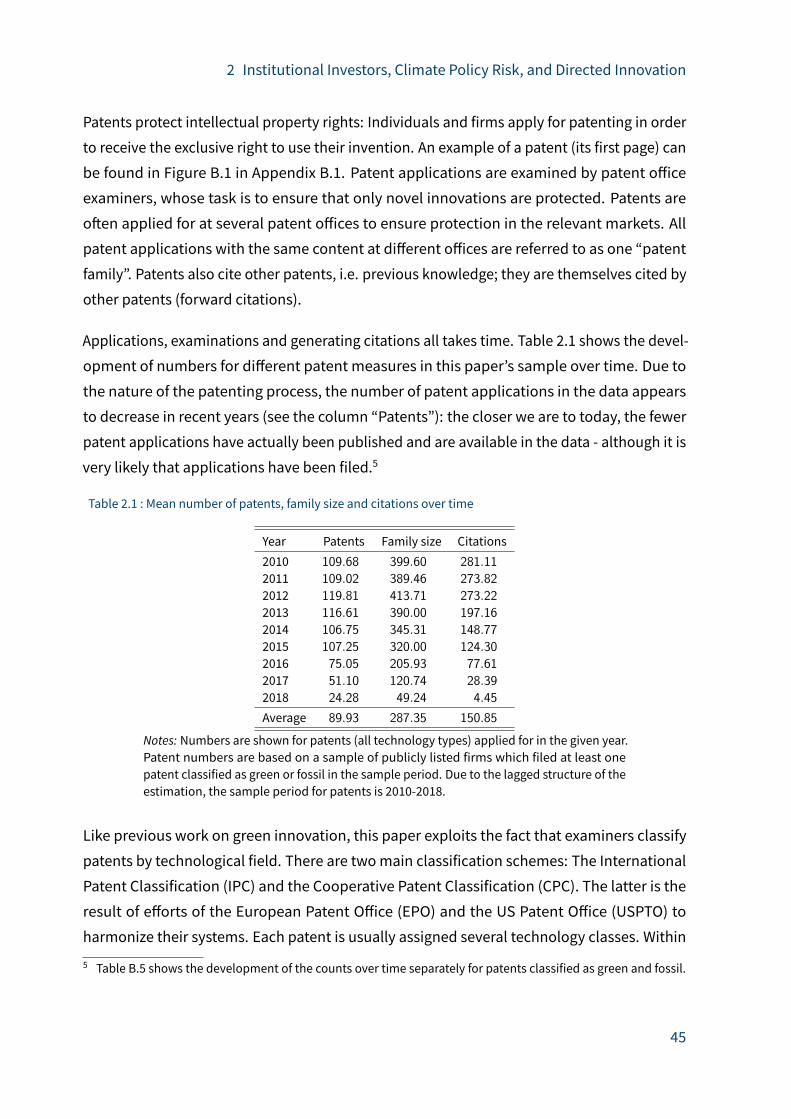
2 Institutional Investors, Climate Policy Risk, and Directed Innovation
Patents protect intellectual property rights: Individuals and firms apply for patenting in order
to receive the exclusive right to use their invention. An example of a patent (its first page) can
be found in Figure B.1 in Appendix B.1. Patent applications are examined by patent o�ice
examiners, whose task is to ensure that only novel innovations are protected. Patents are
o�en applied for at several patent o�ices to ensure protection in the relevant markets. All
patent applications with the same content at di�erent o�ices are referred to as one “patent
family”. Patents also cite other patents, i.e. previous knowledge; they are themselves cited by
other patents (forward citations).
Applications, examinations and generating citations all takes time. Table 2.1 shows the devel-
opment of numbers for di�erent patent measures in this paper’s sample over time. Due to
the nature of the patenting process, the number of patent applications in the data appears
to decrease in recent years (see the column “Patents”): the closer we are to today, the fewer
patent applications have actually been published and are available in the data - although it is
very likely that applications have been filed.5
Table 2.1 : Mean number of patents, family size and citations over time
Year Patents Family size Citations2010 109.68 399.60 281.11
2011 109.02 389.46 273.82
2012 119.81 413.71 273.22
2013 116.61 390.00 197.16
2014 106.75 345.31 148.77
2015 107.25 320.00 124.30
2016 75.05 205.93 77.61
2017 51.10 120.74 28.39
2018 24.28 49.24 4.45
Average 89.93 287.35 150.85
Notes: Numbers are shown for patents (all technology types) applied for in the given year.Patent numbers are based on a sample of publicly listed firms which filed at least onepatent classified as green or fossil in the sample period. Due to the lagged structure of theestimation, the sample period for patents is 2010-2018.
Like previous work on green innovation, this paper exploits the fact that examiners classify
patents by technological field. There are twomain classification schemes: The International
Patent Classification (IPC) and the Cooperative Patent Classification (CPC). The latter is the
result of e�orts of the European Patent O�ice (EPO) and the US Patent O�ice (USPTO) to
harmonize their systems. Each patent is usually assigned several technology classes. Within
5 Table B.5 shows the development of the counts over time separately for patents classified as green and fossil.
45

2 Institutional Investors, Climate Policy Risk, and Directed Innovation
the CPC, a special Y category has been introduced to mark climate-friendly innovations. This
is helpful, but not su�icient, to identify in particular fossil-based patents.
To classify patents as green and fossil, I use a slightly modified version of the classification
by Dechezleprêtre et al. (2017) into clean and dirty patents.6 Examples for fossil transport
categories are F02F, Cylinders, pistons, or casing for combustion engines; arrangements of
sealings in combustion engines, or F02N, Starting of combustion engines. Green transport
includes, for instance, B60K 1, Arrangement or mounting of electrical propulsion units, or
B60L 8, Electric propulsion with power supply from force of nature, e.g. sun, wind. For energy,
corresponding categories would be Y02E 10 (Energy generation through renewable energy
sources) and F23 (Combustion apparatus; combustion processes).
In reality, it is sometimes hard to identify climate-friendly innovation. For instance, there
are inventions that make the use of fossil fuels more e�icient and reduce emissions (Lanzi
et al. 2011). Following Dechezleprêtre et al. (2017), I introduce a third category (in robustness
checks): grey patents. Most of these technologies make combustion (in engines or power
plants) more e�icient, and they are thus a subset of the fossil technologies. In the case of
energy, the grey category also includes the production of fuels of non-fossil origin, e.g. biofu-
els. However, all of these technologies have only limited potential to address technological
risk, which is mainly about the phase-out of fossil-based technologies. Improving existing
technologies at the margin may be successful in the short andmedium run, but does not help
on the way to new, carbon-free systems. An overview of the classifications for transport and
energy-related patents can be found in Tables B.1 and B.2 in Appendix B.1.
The literature agrees that plain patent counts are a very imprecise measure, since patent
quality (or value) is highly skewed (seeAghionet al. 2013, for example). It is therefore important
to account for patent quality. As a first step, I filter patents based on the o�ices where they
were filed. Only patents applied for at the US, EU, or Japanese patent o�ice are considered. In
a second step, patents were filtered to only include granted patents.
In robustness checks, family size and citations are used instead of patent counts. Family size
measures the number of patent o�ices where the patent has been applied for: it is a measure
6 I am using the term fossil instead of dirty due to the focus on climate change and climate risk: CO2, the resultof burning fossil fuels, is not a pollutant, but a greenhouse gas. Climate risk a�ects fossil-based technologies, butdoesnot a�ect all “dirty” technologieswith anyenvironmental externalities. In the samevein, not all technologiesreplacing fossil fuels are automatically “clean” (biomass-fired power plants, for instance, do contribute to airpollution). The term green is therefore used to describe technologies which replace fossil-based technologies.
46

2 Institutional Investors, Climate Policy Risk, and Directed Innovation
for the importance the inventor attaches herself to the patent. If the inventor considers
the invention to be of high value, she will opt to protect (and use) it in many jurisdictions.
Protection at several o�ices incurs direct and administrative costs, so we can assume that it is
a conscious decision of the inventing firm to increase a patent’s family size. Citations, on the
other hand, are ameasure for the relevance that others attach to the patent: if the invention is
cited by other patents, it is su�iciently novel and relevant to spur further innovation. Citations
can be regarded as ameasure for the scientific value of a patent; family size is closer to the
commercial value of the patent.
The censoring issue discussed above is also relevant for the choice of patent measure. As
Table 2.1 shows, the downward trend over time is particularly pronounced for citation counts.
This is not surprising: citations accumulate over time, and patents applied for in 2018 did
not have much time to collect citations. It is generally possible to take care of this issue by
using year fixed e�ects. With count data, however, the amount of zeroes can become quite
large towards the end of the sample, impeding estimations. Family size also decreases faster
over time than plain patent counts - the process of applying for protection at di�erent patent
o�ices takes time as well, and this lag may di�er between technologies and sectors. For this
reason, the standard patent measure used in this paper is the patent count. Family size and
citations are included as a robustness check.
2.3 Empirical approach
2.3.1 Path dependencymodel
The question of this paper is: do institutional investors influence green and/or fossil patenting,
and if yes, in a di�erent way? I therefore test for the impact of the ownership share of institu-
tional investors on green and fossil patenting. The idea for the econometric specification is
inspired by the dynamic path-dependency model by Aghion et al. (2016). In such a model,
the amount of patenting depends on the firm’s own stock of patents; on innovation spillovers
from other firms in the country; and on R&D investments. Since most of the path-dependent
explanatory variables can be derived for green and fossil patent classifications, the model
can be used to separately assess the impact of institutional ownership on green and fossil
patenting. In the following, the subscripts G and F are used to refer to green and fossil
47

2 Institutional Investors, Climate Policy Risk, and Directed Innovation
patents, respectively. For the exposition, green patents are used as the default example for
the dependent variable.7
Following the literature standard, a Poisson specification is used to account for the count
nature of the dependent variable. The model including institutional ownership reads
PATG,it = exp(αG + βG,IOIOit−1 + βG,1 lnKG,it−1 + βG,2 lnKF,it−1
+ βG,3 lnSPILLG,it−1 + βG,4 lnSPILLF,it−1 (2.1)
+ βG,5R&Dit−1 + τG,t + ηG,i + εG,it),
where
– PATG,it is the count of green patents applied for by firm i in year t;
– IOit is the percentage of institutional ownership in firm i in year t− 1;
– KG,it−1 is the firm’s pre-period green patent stock;
– KF,it−1 is the firm’s pre-period fossil patent stock;
– SPILLG,it−1 are country-level green spillovers to firm i in period t− 1;
– SPILLF,it−1 are country-level fossil spillovers to firm i in period t− 1;
– R&Dit−1 are R&D expenditures of firm i in year t− 1;
– τG,t is a year fixed e�ect;
– ηG,i is a firm fixed e�ect; and
– εG,it is an error term.
Institutional ownership is a continuous variable reflecting the relative quantity of institutional
ownership compared to other owners. The literature on institutional owners suggests that
this quantitymakes a qualitative di�erence: (Many) large investors havemore (joint) influence
in proxy votes, conference calls, etc.
7 Further categories are possible, such as green transport patents, grey patents, or total patents; these areintroduced later in the text.
48
2 Institutional Investors, Climate Policy Risk, and Directed Innovation
Essentially, the idea of Equation 2.1 is to single out the influence of institutional ownership
while controlling for already existing knowledge stocks (due to own patenting and spillovers)
and the inherent path dependency. Previous own knowledge on green technologies,KG,it−1
can explain further innovative activities in this direction. SPILLG,it−1 are country-level green
innovation spillovers, based on the assumption that an environment of domestic firms with
knowledge on green technologies is conducive to each firm’s innovation in this direction.
Following Aghion et al. (2016), previous knowledge on fossil technologies and fossil spillovers
are also included (KF,it−1, SPILLF,it−1). This specification is derived from the observation
that many firms with a track record in fossil innovation become active in green innovation:
the technologies are used to serve similar markets, e.g. in the car industry. The construction
of knowledge stocks and spillovers is discussed in detail in section 2.4.
However, patents of course are not generated simply out of previously existing patents. Re-
search and Development is a further obvious part of the firm’s production function of patents
(see also Hall et al. 2005). The inclusion of R&D is particularly useful in the context of this
paper’s research question. R&D expenditure controls for the overall R&D e�orts, so any change
in green or fossil patents we observe can be more clearly interpreted as a directional change,
as opposed to a pure increase.8 In addition, investors may observe R&D e�orts and select into
firms with higher R&D expenditures, expecting larger innovation output; this would cause an
omitted variable bias and an overestimation of investors’ influence.
In robustness checks, twomore control variables are used: Tobin’s q and firm-specific climate
exposure (see section 2.3.5 for details). Onemight think of other firm-specific variables that
are associated with innovation, like financing constraints or firm size. Including measures
for tangibility, leverage, operating revenue, capital-labor ratio, or profits did not significantly
alter the outcome, so the corresponding results are not included in this paper.
8 Contrary to e.g. Aghion et al. (2013) and Hall et al. (2005), this paper uses yearly R&D spendings instead of R&Dstocks. There are twomain reasons for this choice. First, the specification in equation 2.1 already accounts forknowledge stocks, measured by patents. The additional value of the R&D variable (which does not appear in the,otherwise very similar, specification of Aghion et al. 2016) lies in capturing additional innovation e�orts whichare on top of, and separate from, existing knowledge stocks. The second reason is a data concern. Many firms inthe sample have incomplete R&D time series, making the construction of R&D stocks di�icult and error-prone.Sticking with yearly expenditures - and excluding missing firm-years from the analysis - is thus the safer variant.Test regressions (not shown) were run using R&D stocks, without significantly a�ecting results.
49
2 Institutional Investors, Climate Policy Risk, and Directed Innovation
2.3.2 Firm fixed e�ects
Equations 2.1 and 2.3 include firm-level fixed e�ects: Unobserved heterogeneity between
firms needs to be controlled for. In Poisson estimations, the standard approach is to use
the conditional fixed e�ects estimator proposed by Hausman et al. (1984). Put simply, it
conditions on the sample average of the observable variables. The conditional fixed e�ects
estimator requires strict exogeneity of the explanatory variables. This assumption is violated
in a dynamic panel datamodel such as Equation 2.1, which exhibits serial correlation between
innovation stock measures.
Therefore, analternativeapproach tomodelling firm fixede�ects is used: thepre-samplemean
estimator proposed byBlundell et al. (1999) (BGVR), which has been used in the environmental
context e.g. in Nesta et al. (2014). The idea is to condition on the pre-sample mean of the
dependent variable to proxy out the fixed e�ect. This approach is particularly well suited
to patent data, because patent data is typically available in pre-sample years. Blundell et
al. (2002) show that this estimator leads to some bias, but increasing the number of pre-
sample periods (and, to a lesser extent, the number of in-sample periods and the number
of observation units) improves performance. The pre-sample mean enters the estimation in
logged form.
For the research question at hand, the choice of pre-sample periods means dealing with a
trade-o�: more pre-sample information is generally desirable, but green technologies are a
relatively “young” phenomenon. Pre-sample averages of green patenting going back a long
timemay not be useful to reflect current firm characteristics regarding green innovation.9 In
this analysis, the pre-sample average for the years 1995-2008 is used. This is a reasonable
amount of years and at the same time, years with measurable patenting activity in both green
and fossil areas are covered.10
2.3.3 Selection issues and control function
One concern when estimating Equation 2.1 is the selection of investors into firms. The co-
e�icient on institutional ownership share may be biased if investors select into firms with
9 Aghion et al. (2016), who have a sample covering the years 1986 to 2005, argue against the use of the BGVRmethod for this reason: green patenting in the early 1980s was not a good indicator for green patenting in theearly 2000s.10 In a robustness check (not shown), the average for the years 2000-2008 was used, since the data show highergreen patenting activity a�er 2000. The estimation results are virtually the same.
50

2 Institutional Investors, Climate Policy Risk, and Directed Innovation
more expected green (or more fossil) innovation. Most investors use a combination of strate-
gies to deal with climate risk; so it is possible that some investors select the most promising
green-innovation firms, others try to encourage green innovation, and others do both.
I therefore use a source of exogenous variation in institutional ownership: The inclusion of a
firm in a large stock index. It has beenwidely used as an instrument for institutional ownership
(Aghion et al. 2013; Crane et al. 2016; Appel et al. 2016). The idea is that many institutional
investors either directly track such indices, or their managers are benchmarked against them.
Therefore the instrument is expected to be correlated with institutional ownership. For it to
fulfill the exclusion restriction, I need to rule out a relationship between pre-period index
membership on this year’s (green / fossil / total) patenting, controlling for observables. It is
therefore helpful to understand the selection of index members.
Indexmembership is decided on by Index Committees; none of their criteria explicitlymention
innovation. One of themain criteria for inclusion in a large stock index ismarket capitalization.
Also, firms need to fulfil basic eligibility criteria to be added to an index, such as certain thresh-
olds for free-float market capitalization and earnings in the quarters prior to index admission.
Theremay be a concern that a firm’smarket value increases in expectation of future patenting,
and this leads to admission to the index. All estimations control for R&D expenditures and thus
for the observable part of innovation activities that may result in patents. I also show in Table
B.12 that Tobin’s q, a measure for above-fundamental market valuation, is not a significant
predictor of innovation. In the first-stage regressions, the coe�icient of Tobin’s q is insignificant
aswell, implying that thismeasure ofmarket valuation does not a�ect institutional ownership,
controlling for other observables. It has also been shown that markets price in most of the
value of patents at a later stage: when a patent is granted (Kogan et al. 2017).11
Moreover, Index Committees do not simply decide based on fixed criteria. For instance, it
is the explicit goal of the S&P 500 Index to be representative of the US economy in terms
of sector coverage. Also, if a current index member does not fulfil the eligibility criteria any
more, this does not automatically lead to exclusion. Index managers are interested in a stable
11 Considering the eligibility criteria, the relationship between high free-float (with, e.g., low family or manage-ment ownership) and innovation is not a priori clear, and the evidence on family or management ownership andinnovation is mixed (Munari et al. 2010; Schmid et al. 2014; Beyer et al. 2012; Ortega-Argilés et al. 2005). Lookingat earnings, it is di�icult to think of a reason why higher earnings would be followed by patent filings, given thatthe required R&D expenditures reduce earnings.
51

2 Institutional Investors, Climate Policy Risk, and Directed Innovation
composition of the index. This discretion provides another source of variation that is not
related to other firm variables.
I define the instrument indexmemberit as a dummy equal to one if a firm was a member
of the S&P 500, the STOXX Europe 600 and/or the S&P Global 1200 index in year t. These
indices cover a wide range of countries, while still being exclusive enough to have explanatory
power. Given the nonlinear model, the instrument enters the estimation in a control function
approach (Wooldridge 2010). In the first stage (OLS), institutional ownership is regressed
on the instrument and all control variables of the second stage. The residuals from this
estimation - i.e., the part of institutional investors’ ownership that cannot be explained by
the instrument - are then included as a control variable in the second-stage regression. As a
result, the coe�icient on IOit reflects the e�ect of the part of institutional ownership that is
due to the index membership of the firm.
2.3.4 Heterogeneity of sectors and institutional owners
Themeasurement of green and fossil patents is noisy. Some of the noise can be addressed
by di�erentiating between sectors. The transport and the energy sector are quite di�erent,
and it is well possible that innovation and patents play a di�erent role in the two sectors. For
capital-heavy energy firms, their fossil fuel reserves or power generating infrastructure are
important assets which are directly a�ected by climate policy, whereas intangible assets such
as patents are likely to play a smaller role. In the transport industry, by contrast, knowledge
and innovation are relatively more important.
In separate regressions, Equation 2.1 is modified accordingly to reflect green/fossil transport
and energy patents separately. The estimated equation for green transport patents, denoted
byGT , thus reads
PATGT,it = exp(αGT + βGT,IOIOit−1 + βGT,1 lnKGT,it−1 + βGT,2 lnKFT,it−1
+ βGT,3 lnSPILLGT,it−1 + βGT,4 lnSPILLFT,it−1 (2.2)
+ βGT,3R&Dit−1 + τGT,t + ηGT,i + εGT,it).
Models for fossil transport and green/fossil energy patents can be derived analogously.
52

2 Institutional Investors, Climate Policy Risk, and Directed Innovation
Similarly, there is noise in the measurement of institutional ownership: there are many di�er-
ent typesof institutional investors, and theymayhavequite di�erent investment/ engagement
strategies, time horizons, or environmental concerns. Oneway to deal with the noise is to look
at these di�erent types specifically. The literature on institutional owners’ engagement sug-
gests some time-invariant types which are expected to have long-term investment strategies
(Hsu and Liang 2017; Borochin et al. 2020). Insurance companies and pension funds are prime
examples. Government ownership is also typically long-term and stable; state-owned enter-
prises have been shown to perform better environmentally. Moreover, domestic investors
(sharing the portfolio firm’s headquarter country) may have better opportunities to engage.
In the context of sustainable finance, it is also possible to exploit a time-varying investor
type, namely signatories of the UN Principles for Responsible Investment (UN PRI) initiative
(see also Dyck et al. 2019). Principle 2, for instance, reads: “We will be active owners and
incorporate ESG issues into our ownership policies and practices.”12 The UN PRI sees itself
as “the world’s leading proponent of responsible investment”. The initiative was launched in
2006 and currently has more than 3,000 signatories. With their membership, investors declare
their willingness to implement the six principles.
In the literature on institutional investors, the role of engagement has been very prominently
discussed in the context of the big passive index funds. Instead of actively managing funds,
thesehold relatively fixedpositions as theyaremirroring certain stock indices. Thismeans they
cannot easily sell their positions, and some argue that this limits their shareholder power. On
the other hand, they have an incentive to use engagement, since this is the only way they can
manage risk. A growing literature showshow thebig indexers use their voting power in director
(re-)elections and other governance choices (Fichtner et al. 2017; Appel et al. 2016), support
activists (Appel et al. 2018), and have an influence on firms’ emission reductions. In this light,
direct engagement activities with management seem to be a successful strategy even, or
particularly, for big “passive” investors. Therefore, the “Big Three” index fund investment
companies (BlackRock, Vanguard, and State Street) are defined as another investor type.
To account for investor type heterogeneity, the variable IO from Equation 2.1 can be replaced
by specific sub-groups of institutional owners: government (GOV ), insurance and pension
12 Stated on the PRI website, see https://www.unpri.org/pri.
53

2 Institutional Investors, Climate Policy Risk, and Directed Innovation
funds (INP ), domestic owners (DOM ), signatories of the UN Principles for Responsible
Investment (UN PRI) initiative (PRI), and “Big Three” investment companies (BIG3).13
2.3.5 Informational value of nonsignificant results
Aswill be shown indetail in section2.5onResults, I donot finda statistically significant e�ect of
institutional ownership on green or fossil innovation. I therefore conducted some additional
estimations, which are not robustness checks in the typical sense. The usual robustness
checks aim to rule out a type I error, i.e., falsely rejecting the null hypothesis. The additional
estimations presented here are rather attempts to rule out a type II error: failure to reject the
null despite an actually existing relationship. Abadie (2020) argues that insignificant estimates
can be highly informative: it is interesting to learn that a previously expected relationship
does not exist. The question is whether insignificant estimates are meaningful, i.e. can be
interpreted as “no e�ect”. Type II errors are most likely to result from data quality or research
design issues. The two specifications presented in the following aim to answer the question
whether research design or data quality are a concern.14
Institutional ownership and total innovation A first check concerns the overall setup of
the model, and the su�iciency of data variation in the institutional ownership variable. The
relationship between institutional ownership and patenting is an established result (Aghion
et al. 2013). If the data andmodel usedhere cannot confirm this result, the researchdesign and
/ or the measurement of the institutional ownership would need to be re-examined. Equation
2.3 tests whether institutional ownership a�ects total innovation (denoted byA):
PATA,it = exp(αG + βA,IOIOit−1 + βA,1 lnKA,it−1 + βA,2 lnSPILLA,it−1
+ βA,3R&Dit−1 + τA,t + ηA,i + εA,it). (2.3)
In this case, previous own knowledge and spillovers in terms of all technologies are included
as explanatory variables. In a robustness check, Tobin’s q is also included. Tobin’s q is defined
as (marketcapitalization+totaldebt)/totalassets and is therefore ameasure of themarket’s
future expectations deviating from current fundamentals. As argued in Aghion et al. (2013),
13 Further investor type definitions are possible (see section B.2), but are less likely to be relevant in a climatecontext, and their results are not shown in the paper.14 In addition, section 2.5.1 provides results for some specification alterations that also partly address thisquestion. Section 2.6 provides a general discussion of the plausibility of the results.
54

2 Institutional Investors, Climate Policy Risk, and Directed Innovation
themarket valuation of firmsmay be an omitted variable in a regression involving institutional
ownership and innovation. It is correlated with the number of patents and could be correlated
with institutional ownership, since institutional owners are more likely to invest in firms with
high market valuation.
Firm-specific climate concerns: “climate exposure” The second approach addresses the
question whether there is su�icient statistical power in the dependent variable(s), i.e. in the
counts of green and fossil patents; it also addresses the question whether the degree to which
firms are a�ected by climate issues play a role in explaining innovation. The degree to which
firms are a�ected by, or concerned about, climate issues varies between firms and over time.
Previous research has shown that firms facing higher fuel taxes tend to patent more in green
technologies, and less in fossil technologies (Aghion et al. 2016). It is logical to test whether
the panel used in this paper can confirm the relationship between firm-level climate policy
impacts and the direction of innovation.
In the context of the research question on institutional ownership and risk from future climate
policies, a newly developedmeasure is particularly useful: “climate exposure”, an indicator
derived from conference calls betweenmanagers and investors. This indicator, developed by
Sautner et al. (2020b), measures the relative frequency with which climate-related issues are
mentioned in these conference calls.
As climate-related issues can be quite broad and diverse, four di�erent sets of bigrams (expres-
sions) are used: one for broadly defined climate change aspects (“climate change exposure”
or “exposure to a climate change-related shock”), and three for more specific topics. These
are physical, regulatory, and opportunity shocks, relating to physical climate change-induced
events (such as heatwaves or sea-level rise), regulatory changes (such as CO2 pricing), and
opportunities (capturing opportunities related to climate change issues, mostly green tech-
nologies). Since physical shocks are unlikely to influence green or fossil patenting (the patent
classifications do not include technologies for adaptation to climate change), the measures
used in this paper are “climate change exposure”, “regulatory exposure”, and “opportunity
exposure”. Table 2.2 shows the top 10 bigrams contributing to general climate exposure,
regulatory exposure, and opportunity exposure, respectively.
To interpret the exposure measures, it is helpful to think of them as “firm-level exposure to a
particular shock”, where the shock can be positive or negative. For opportunity shocks, on
55
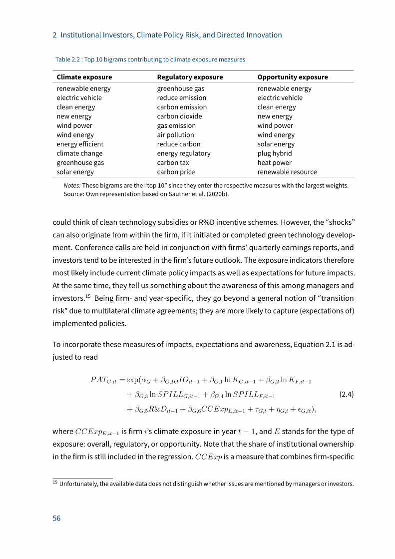
2 Institutional Investors, Climate Policy Risk, and Directed Innovation
Table 2.2 : Top 10 bigrams contributing to climate exposure measures
Climate exposure Regulatory exposure Opportunity exposurerenewable energy greenhouse gas renewable energyelectric vehicle reduce emission electric vehicleclean energy carbon emission clean energynew energy carbon dioxide new energywind power gas emission wind powerwind energy air pollution wind energyenergy e�icient reduce carbon solar energyclimate change energy regulatory plug hybridgreenhouse gas carbon tax heat powersolar energy carbon price renewable resource
Notes: These bigrams are the “top 10” since they enter the respective measures with the largest weights.Source: Own representation based on Sautner et al. (2020b).
could think of clean technology subsidies or R%D incentive schemes. However, the “shocks”
can also originate from within the firm, if it initiated or completed green technology develop-
ment. Conference calls are held in conjunction with firms’ quarterly earnings reports, and
investors tend to be interested in the firm’s future outlook. The exposure indicators therefore
most likely include current climate policy impacts as well as expectations for future impacts.
At the same time, they tell us something about the awareness of this amongmanagers and
investors.15 Being firm- and year-specific, they go beyond a general notion of “transition
risk” due to multilateral climate agreements; they are more likely to capture (expectations of)
implemented policies.
To incorporate these measures of impacts, expectations and awareness, Equation 2.1 is ad-
justed to read
PATG,it = exp(αG + βG,IOIOit−1 + βG,1 lnKG,it−1 + βG,2 lnKF,it−1
+ βG,3 lnSPILLG,it−1 + βG,4 lnSPILLF,it−1 (2.4)
+ βG,5R&Dit−1 + βG,6CCExpE,it−1 + τG,t + ηG,i + εG,it),
where CCExpE,it−1 is firm i’s climate exposure in year t − 1, and E stands for the type of
exposure: overall, regulatory, or opportunity. Note that the share of institutional ownership
in the firm is still included in the regression. CCExp is a measure that combines firm-specific
15 Unfortunately, the available data does not distinguishwhether issues arementioned bymanagers or investors.
56
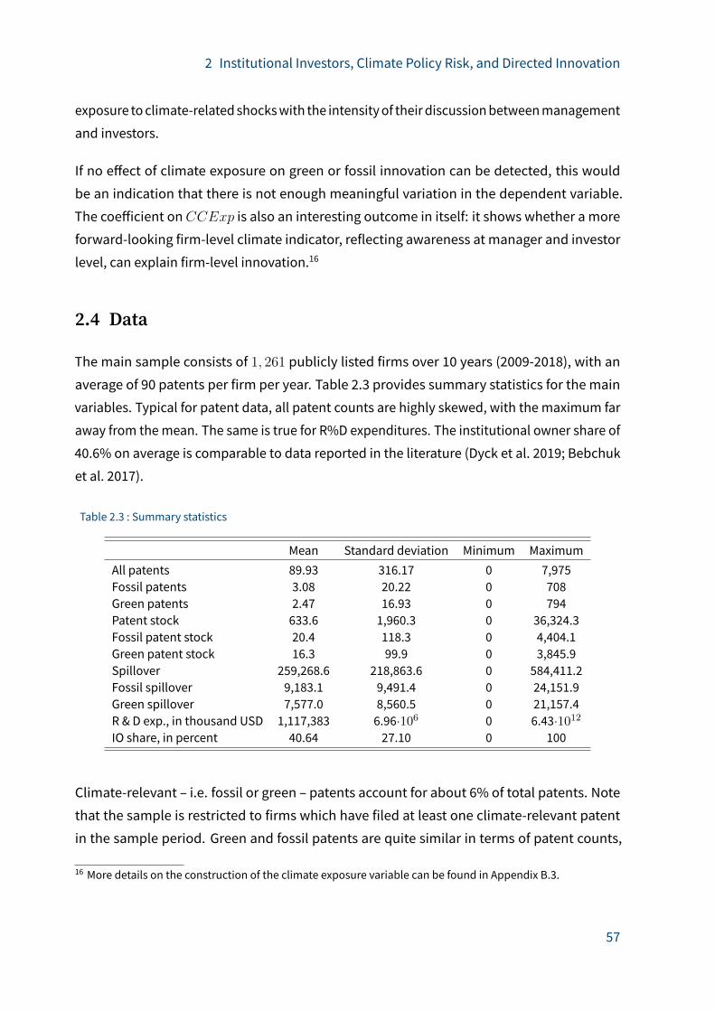
2 Institutional Investors, Climate Policy Risk, and Directed Innovation
exposure toclimate-related shockswith the intensityof their discussionbetweenmanagement
and investors.
If no e�ect of climate exposure on green or fossil innovation can be detected, this would
be an indication that there is not enough meaningful variation in the dependent variable.
The coe�icient onCCExp is also an interesting outcome in itself: it shows whether a more
forward-looking firm-level climate indicator, reflecting awareness at manager and investor
level, can explain firm-level innovation.16
2.4 Data
The main sample consists of 1, 261 publicly listed firms over 10 years (2009-2018), with an
average of 90 patents per firm per year. Table 2.3 provides summary statistics for the main
variables. Typical for patent data, all patent counts are highly skewed, with the maximum far
away from themean. The same is true for R%D expenditures. The institutional owner share of
40.6% on average is comparable to data reported in the literature (Dyck et al. 2019; Bebchuk
et al. 2017).
Table 2.3 : Summary statistics
Mean Standard deviation Minimum MaximumAll patents 89.93 316.17 0 7,975Fossil patents 3.08 20.22 0 708Green patents 2.47 16.93 0 794Patent stock 633.6 1,960.3 0 36,324.3Fossil patent stock 20.4 118.3 0 4,404.1Green patent stock 16.3 99.9 0 3,845.9Spillover 259,268.6 218,863.6 0 584,411.2Fossil spillover 9,183.1 9,491.4 0 24,151.9Green spillover 7,577.0 8,560.5 0 21,157.4R & D exp., in thousand USD 1,117,383 6.96·106 0 6.43·1012IO share, in percent 40.64 27.10 0 100
Climate-relevant – i.e. fossil or green – patents account for about 6% of total patents. Note
that the sample is restricted to firms which have filed at least one climate-relevant patent
in the sample period. Green and fossil patents are quite similar in terms of patent counts,
16 More details on the construction of the climate exposure variable can be found in Appendix B.3.
57
2 Institutional Investors, Climate Policy Risk, and Directed Innovation
patent stocks and spillovers, with green innovation always slightly below fossil. Table B.4 in
Appendix B.4 shows the respective averages for family size and citations.
Themain data source for patents, firms and ownership is Orbis and Orbis Intellectual Property,
o�ered by Bureau van Dijk (BvD). Orbis provides information onmore than 300million compa-
nies worldwide, with the data including standardized financials, ownership links, andmore.
Ownership data Data on ownership is recorded in the Orbis Historical Database. It provides
links between firms and their shareholders, listing the respective ownership shares. The
ownership data is collected from various sources, leading to over-reporting in the dataset.
Extensive manual checks were done to rule out duplicates. In case a duplicate was identified,
preference was given to the most recent reporting, to the most comprehensive (and thus
consistent) data sources,17 or to the parent company in case of holding reportings.
The ownership data allows to distinguish between di�erent investor types based on their
NACE codes and BvD classifications. Details on the mapping can be found in section B.2 in
Appendix B.2. In addition, the headquarter country of each investor is recorded in the dataset,
allowing to identify domestic investors.
Information on the investors’ signature dates in the United Nations Principles for Responsible
Investment initiative is from the PRI’s website.18 The PRI signatories are only available by
name. They were matched to the investor dataset using a fuzzy matching approach as a first
step; this was augmented with amanual check of the matches. In some cases, it is di�icult
to find out from an investor’s PRI reporting which parts of the company can be counted as PRI
signatories. Thematches were checked with the greatest care possible, but somemismatches
can not be ruled out.
Summary statistics for the di�erent owner types can be found in Table B.6 in Appendix B.4.
The average share of governments and Big Three investors is lowest; the ownership share of
domestic owners is the highest of all types used (27.7% on average, more than half of total
17 Themost prevalent data source, and therefore most consistent across firms and years, is Factset. Factset isan independent data provider collecting data on large investors’ holdings, based on filings with national stockexchange supervision authorities. Themost well-known are the so-called “13F” filings, which are mandatoryfor investors in US-listed firms when their share crosses a certain threshold. Unfortunately, the sample couldnot be restricted to Factset alone, since in many cases important investors appeared under di�erent sources indi�erent years in the same firm.18 https://www.unpri.org/signatories/signatory-directory
58
2 Institutional Investors, Climate Policy Risk, and Directed Innovation
institutional ownership, and with a maximum value of 100%). In the shares of governments
as well as insurance and pension fund companies, the variation is somewhat larger than for
the other groups.
Patent data Orbis Intellectual Property is the result of a matching between PATSTAT (a
worldwide patent database run by the European Patent O�ice) and Orbis. Linked to company
IDs, it provides rich information on each patent, including its classification, date of publication,
and application o�ices. The dataset in this paper consists of all patents which were filed at
the European Patent O�ice (EPO), the US Patent and Trademark O�ice (USPTO), the Japanese
Patent O�ice (JPO), or the World Intellectual Property Organization (WIPO) in the relevant
period; whichwere ultimately granted; andwhich can be linked to a listed firm (either through
direct or indirect ownership, currently or formerly).
The database o�ers information of the applicant firm(s), current direct owner(s), and current
indirect owner(s) of the patents. The patents were thus assigned to firms based on the original
applicant (or several original applicants), if this original applicant is a listed firm. If the original
applicant is not listed, but the current indirect owner is (and if there has been no ownership
change), then the patent is assigned to the indirect owner. Since the database does not easily
allow to track indirect ownership of firms over time, cases with changes in ownership are not
assigned an indirect owner. Changes in ownership are determined by a) using the label “with
ownership change” from Orbis, and b) by ensuring that the data lists the applicant also as
the direct owner.
The estimations use patent applications (a flow) as the dependent variable, but patent stocks
as explanatory variables. In line with the literature, these patent stocks are calculated using
the perpetual inventory method. Firm i’s green patent stock in year t,KG,it, is equal to the
discounted flow of green patents in the previous years:
KG,it = PATG,it + (1− ρ)KG,it−1, (2.5)
and symmetrically for fossil (KF,it) or all patents (KA,it), respectively. A discount rate of
ρ = 0.15 is used, which is in themedium range of depreciation rates for intellectual capital
used in the literature.19
19 For example, Aghion et al. (2016) use 20%; Peri (2005) uses 10%, Hall et al. (2005) and Cockburn and Griliches(1988) use 15%.
59

2 Institutional Investors, Climate Policy Risk, and Directed Innovation
Spillovers are accounted for in a relatively straightforward way. A firm’s green spillover at time
t is equal to the sum of green patents applied for in the firm’s country c at time t, minus the
firm’s own green patent applications in that year:
SPILLG,it =∑j∈c
PATG,jt − PATG,it. (2.6)
In all expressions involving the log of a number of patents (i.e. lnK, lnSPILL, as well as the
pre-sample mean), I follow the literature standard of replacing zeroes by an arbitrary small
constant and including dummies for the number of patents being zero (Aghion et al. 2016;
Blundell et al. 1999).
Firm data Firm-level data on R&D expenditures and Tobin’s q is from the Orbis Historical
Database. BvD firm-level data is mainly sourced from companies’ mandatory filings. For com-
panies with subsidiaries, sometimes both unconsolidated and consolidated (including sub-
sidiaries) reporting is available. Whenever a company appears as an indirect patent applicant
(or as both direct and indirect), and both filing versions are available, then the consolidated
reporting version is used. In further regressions, more firm-level characteristics were used as
control variables (such as operating revenue, capital-labor ratio), but as they did not alter the
results, the respective regressions are not shown in the paper.
Firm-level data is augmented by other sources: Thomson Reuters Datastreamwas used to
extract time series of index constituents of the STOXX Europe 600 and S&P Global 1200 indices.
The time series of the S&P 500 is fromWharton Research Data Services (WRDS).
In addition, the Sautner et al. (2020a) data was merged to the firms to cover firm-level climate
exposure and its recognition with managers and investors. Since all firms in the sample are
publicly listed, ISINs (International Securities Identification Numbers) of their traded shares
could be used to match the firms. The climate change exposure data is limited in terms of
firm coverage and in terms of time series coverage per firm, reducing the sample size of the
dataset to roughly half of the original dataset. Summary statistics for the reduced sample can
be found in Table B.7 in Appendix B.4. Firms in the climate exposure sample have filed more
patents (in all categories), have higher R&D expenditures, and a higher institutional owner
share than the average of the full sample.
60

2 Institutional Investors, Climate Policy Risk, and Directed Innovation
2.5 Results
2.5.1 Institutional owners and climate-relevant innovation
Table 2.4 show the main results for Equation 2.1, separately for green and fossil patents. For
each estimation, the first stage of the control function approach is shown in an extra column.
As can be seen from columns 2 and 4, the indexmember instrument is positive and significant:
Institutional investors own about 2.3 percentage pointsmore stocks inmembers of large stock
indices than we would expect from other observables.
Table 2.4 : Green and fossil patents
(1) (2) (3) (4)Model Poisson OLS (first stage) Poisson OLS (first stage)Dep. var. Green patents L.IO share Fossil patents L.IO shareL.IO share 0.0227 0.0103
(0.0561) (0.0387)L.Own stock green 1.464∗∗∗ -1.341∗∗∗ 0.0224 -2.550∗∗∗
(0.104) (0.493) (0.107) (0.268)L.Own stock fossil 0.134∗∗ -1.076∗∗∗ 1.321∗∗∗ -2.556∗∗∗
(0.0617) (0.264) (0.122) (0.524)L.Green spillover 0.544 -20.05∗∗∗ 0.212 -20.01∗∗∗
(1.141) (0.788) (0.783) (0.781)L.Fossil spillover -0.515 20.24∗∗∗ -0.223 20.15∗∗∗
(1.147) (0.791) (0.787) (0.783)L.R and D exp. 0.0131 3.962∗∗∗ 0.0943 4.012∗∗∗
(0.238) (0.170) (0.171) (0.171)L.Index member 2.286∗∗∗ 2.291∗∗∗
(0.705) (0.705)Observations 8621 8621
Notes: Robust standard errors in parentheses. Knowledge stocks, spillovers and R&D expenditures are inlogs. Estimation period is 2009-2018. All regressions include year fixed e�ects and firm fixed e�ects using theBGVRmethod. Significance levels are indicated as ∗ p < 0.1, ∗∗ p < 0.05, ∗∗∗ p < 0.01.
A�er controlling for their endogeneity, the influence of institutional investors on both green
and fossil patenting is positive, but statistically indistinguishable from zero. Based on the
aggregate measures of green and fossil patents as well as institutional ownership used here, I
cannot say that there is any causal relationship between institutional ownership and green or
fossil patenting.
The results do, however, qualitatively confirm the findings from Aghion et al. (2016) on path
dependency: A higher fossil (green) patent stock significantly increases the probability of filing
another fossil (green) patent. The data also confirm another result, namely that a firm’s fossil
61
2 Institutional Investors, Climate Policy Risk, and Directed Innovation
knowledge stock is also associated with more green patenting, whereas the green knowledge
stock does not a�ect fossil patent applications. Overall, the path dependency model seems
to fit the data quite well. The very simple spillover measure applied in this estimation is not
significant though, neither for green nor for fossil patenting.
Accounting for sector heterogeneity As mentioned in section 2.3.4, the aggregate mea-
sures on green and fossil patenting may hide some important di�erences between the energy
and the transport sector. Most likely, (green) innovations play a larger role in the transport
sector than in the capital-heavy energy sector. Moreover, product market competition likely
di�ers between these sectors, with implications for the innovation process and ownership.20
Table 2.5 therefore shows results for green and fossil patents in the transport (columns 1
and 2) and energy sector (columns 3 and 4) separately. In all cases, the coe�icient on institu-
tional ownership is small or even negative, and the null hypothesis of it being zero cannot be
rejected.
Again, the general path dependency model performs well: Both green and fossil transport
knowledge stocks influence green transport patenting positively, while green transport knowl-
edge is not associated with an increase in fossil transport patenting – this is in line with the
results in Aghion et al. (2016), which are in fact focused on the transport sector. In the case of
energy-related patents, the same pattern can be observed with very similar coe�icients. This
suggests that the specification in Equation 2.2 works well for both sectors.
Accounting for investor heterogeneity The insignificant influence of institutional owners
on the direction of innovation may also be due to the underlying heterogeneity of investors,
as mentioned in section 2.3.4.21 Not all institutional owners invest with a long time horizon,
not all of them have voiced an interest in climate change issues, and not all of them are prone
to engage. The results for the e�ect of di�erent types of investors on green innovation can be
found in Table 2.6. This table only shows the coe�icient for investor type ownership; the full
tables for green as well as fossil innovation can be found in Appendix B.5 (Tables B.10 and
B.11).
20 For the relevance of competition in the context of (green) innovation and ownership, see e.g. Aghion et al.(2005), Atanassov (2013), Borochin et al. (2020), Lambertini et al. (2017), and Nesta et al. (2014).21 For summary statistics for the respective owner types, please refer to Table B.6.
62
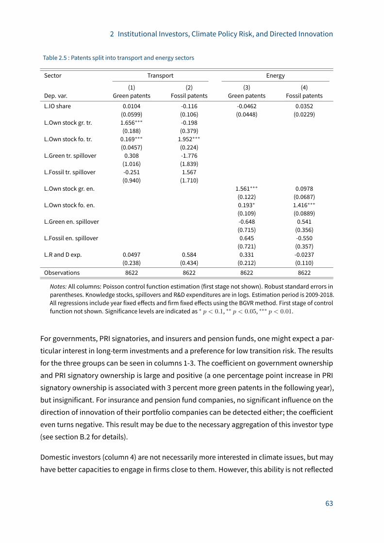
2 Institutional Investors, Climate Policy Risk, and Directed Innovation
Table 2.5 : Patents split into transport and energy sectors
Sector Transport Energy
(1) (2) (3) (4)Dep. var. Green patents Fossil patents Green patents Fossil patents
L.IO share 0.0104 -0.116 -0.0462 0.0352(0.0599) (0.106) (0.0448) (0.0229)
L.Own stock gr. tr. 1.656∗∗∗ -0.198(0.188) (0.379)
L.Own stock fo. tr. 0.169∗∗∗ 1.952∗∗∗
(0.0457) (0.224)L.Green tr. spillover 0.308 -1.776
(1.016) (1.839)L.Fossil tr. spillover -0.251 1.567
(0.940) (1.710)L.Own stock gr. en. 1.561∗∗∗ 0.0978
(0.122) (0.0687)L.Own stock fo. en. 0.193∗ 1.416∗∗∗
(0.109) (0.0889)L.Green en. spillover -0.648 0.541
(0.715) (0.356)L.Fossil en. spillover 0.645 -0.550
(0.721) (0.357)L.R and D exp. 0.0497 0.584 0.331 -0.0237
(0.238) (0.434) (0.212) (0.110)Observations 8622 8622 8622 8622
Notes: All columns: Poisson control function estimation (first stage not shown). Robust standard errors inparentheses. Knowledge stocks, spillovers and R&D expenditures are in logs. Estimation period is 2009-2018.All regressions include year fixed e�ects and firm fixed e�ects using the BGVRmethod. First stage of controlfunction not shown. Significance levels are indicated as ∗ p < 0.1, ∗∗ p < 0.05, ∗∗∗ p < 0.01.
For governments, PRI signatories, and insurers and pension funds, onemight expect a par-
ticular interest in long-term investments and a preference for low transition risk. The results
for the three groups can be seen in columns 1-3. The coe�icient on government ownership
and PRI signatory ownership is large and positive (a one percentage point increase in PRI
signatory ownership is associated with 3 percent more green patents in the following year),
but insignificant. For insurance and pension fund companies, no significant influence on the
direction of innovation of their portfolio companies can be detected either; the coe�icient
even turns negative. This result may be due to the necessary aggregation of this investor type
(see section B.2 for details).
Domestic investors (column 4) are not necessarily more interested in climate issues, but may
have better capacities to engage in firms close to them. However, this ability is not reflected
63

2 Institutional Investors, Climate Policy Risk, and Directed Innovation
Table 2.6 : Special investor types and green patenting
(1) (2) (3) (4) (5)
L.Gov. share 0.0342(0.0882)
L.PRI sig. share 0.0343(0.0796)
L.Ins.& pens. fd. share -0.121(0.298)
L.Domestic owner share -0.0210(0.0505)
L.Big 3 share 0.0257(0.0610)
Observations 8622 8622 8622 8622 8622
Notes: Dependent variable: Green patents. All columns: Poisson control function estimation (first stage notshown). Robust standard errors in parentheses. Estimation period is 2009-2018. All regressions include yearfixed e�ects and firm fixed e�ects using the BGVRmethod. Further regressors not shown. Significance levelsare indicated as ∗ p < 0.1, ∗∗ p < 0.05, ∗∗∗ p < 0.01.
in the results, where the coe�icient on domestic investors is insignificant and even negative.
Column 5 reports results with the share of the “Big Three” index fundmanagers (BlackRock,
Vanguard, and State Street) as the dependent variable. All of them have voiced concern about
climate risk.22 Given their limited ability to influence their risk via selection, the engagement
channel might be particularly important for them. Although the Big Three have been shown
to contribute to emission reductions of firms (Azar et al. 2020), the insignificant coe�icient
suggests that their engagement activities donot yet address technological risk in ameasurable
way.
In summary, the findings for all of these investor types are the same as for the aggregate: no
statistically significant e�ect of a larger ownership share of any particular investor type on
green or fossil patenting can be detected.
Some further specification alterations Tables B.8 and B.9 in Appendix B.5 show results
for some basic changes in the specification.
One could argue that institutional investors have a particular interest to direct innovation
towards high-quality green patenting. Despite focusing on patents which are ultimately
22 In fact, they are all PRI signatories, implying some overlap between the Big Three type and the PRI signatorytype.
64

2 Institutional Investors, Climate Policy Risk, and Directed Innovation
granted, patent counts may not capture patent quality su�iciently. As described in section
2.2, family size could be a useful measure in the context of this analysis: it captures the firm’s
expected commercial value of the patent, and it su�ers less from sample censoring than
citations. Columns 1 and 2 of Table B.8 show the impact of institutional ownership on the
family size of green and fossil patents, respectively. The coe�icients decrease in size and
remain insignificant. Owners’ concern with innovative quality does not seem to be the main
issue.
Another concern could be that the dichotomy of green and fossil technologies does not fully
capture climate-relevant innovation. There is also the interimcaseofgrey patents, whichmake
fossil technologiesmore e�icient and thus reduce emissions. It is possible that investors value
the (potentially) low cost and low risk character of these types of incremental innovations. As
column 3 in Table B.8 shows, this hypothesis is not supported by the data.
One of the main arguments why institutional owners can exert influence on firms is that their
large stakes implymore concentrated ownership. Itmight therefore only be the largest owners
that drive successful engagement. In columns 1 and 2 of Table B.9, the share of institutional
ownership is replaced by the share of the five largest owners. The coe�icient is negative in
both cases, and insignificant.
It is also possible that the influence of institutional investors takes longer to materialize
than one year.23 Columns 3 and 4 of Table B.9 therefore show results for a two-year lag of
institutional ownership, IOit−2. The coe�icient on green patenting gets larger compared to
the baseline, and the coe�icient on fossil patenting gets smaller, indicating that there might
be some truth in this argument; however, the coe�icients are still insignificant.
2.5.2 Institutional owners and total innovation
From the results presented so far, the interim conclusion is that there is no evidence of institu-
tional owners influencing the direction of innovation in firms. However, this lack of significant
e�ects on climate-related patenting might be due to specification or data issues that have
nothing to do with the green and fossil patents themselves. Can the data andmodel identify
any e�ect of institutional ownership on innovation? To answer this question, equation 2.3 is
estimated, covering all patents.
23 Atanassov (2013), for instance, uses a time lag of two years.
65

2 Institutional Investors, Climate Policy Risk, and Directed Innovation
Themain results from these regressions (omitting all explanatory variables except institutional
ownership from the table24) are presented in Table 2.7. In this case, institutional ownership
has a positive and significant e�ect on total innovation: A ten percentage point increase in
institutional ownership leads to 11.4%more patent filings. At the mean, this would mean a
shi� from 40.6 to 50.6% in institutional ownership resulting in an increase from 89.9 to 100.2
patents. Despite a di�erent model equation, this result is quite close to the findings in Aghion
et al. (2013), where the Poisson specification delivers coe�icients between 0.007 and 0.010.
It is surprisingly robust over a wide range of specifications. Column 1 shows the baseline
Poisson control function regression of equation 2.3, which is comparable to the estimations
in Tables 2.4 and 2.5. Column 2 introduces two-way clustering of standard errors at the 4-digit
NACE code and country level.
In column 3, an additional control variable is introduced: Tobin’s q, a measure of the market’s
future expectations deviating from current fundamentals. It could bias the results, since it
might be correlated with patents as well as institutional ownership. However, controlling for
Tobin’s q hardly changes the coe�icient on institutional ownership; as shown in Table B.12,
the coe�icient on Tobin’s q is also insignificant.
In columns 4 and 5, robustness with respect to the choice of patent count measure is tested.
Column4uses family-weightedpatents inall patent variables, andcolumn5uses citations. The
citation-based regression is the only onewithout a significant e�ect of institutional ownership.
As explained in section 2.2, citations su�er particularly from sample attrition due to the time
line of the patenting and citation process. Also, the number of citations can be zero, which
leads to an excessive amount of zeroes especially towards the end of the sample (whereas the
family size of each patent is always at least 1, the patent itself). Finally, column 6 changes the
estimation model from Poisson to negative binomial, which is sometimes recommended in
case of overdispersion of the data.25 The coe�icient on institutional ownership gets smaller,
but is still significant.
From Table 2.7, we can conclude that a connection between institutional ownership and
innovation can be establishedwith the given data andmodel. Looking at the combined results
on carbon-relevant and total patenting, investors appear to encourage overall innovation,
24 The complete results are available in Appendix B.5, Table B.12.25 Note that the GMM-based ivpoisson estimator implemented in Stata works for any exponential model withmultiplicative error and is robust to overdispersion. The negative binomial estimator, on the other hand, is lessrobust to misspecification.
66

2 Institutional Investors, Climate Policy Risk, and Directed Innovation
Table 2.7 : Institutional investors and total patents
(1) (2) (3) (4) (5) (6)Model Poisson Poisson Poisson Poisson Poisson Neg. bin.Dep. var. Patents Patents Patents Family size Citations Patents
L.IO share 0.0114∗∗∗ 0.0114∗∗ 0.0110∗ 0.0129∗∗ -0.0258 0.00671∗∗
(0.00348) (0.00481) (0.00603) (0.00624) (0.0177) (0.00310)Clustered SEs no yes yes yes yes yesAdd. control no no yes no no noObservations 8622 8622 8040 8622 8622 8622
Notes: All estimations use a control function approach (first stage not shown). “Add. control” refers to theinclusion of Tobin’s q as an additional control variable. Robust standard errors in parentheses. In the Poissoncontrol function estimations starting in column 2, standard errors are two-way clustered at the 4-digit NACEcode and country level. In the negative binomial control function estimation, standard errors are clusteredat the 4-digit NACE code level. Knowledge stocks, spillovers and R&D expenditures are in logs. Estimationperiod is 2009-2018. All regressions include further controls, year fixed e�ects, and firm fixed e�ects usingthe BGVRmethod. Significance levels are indicated as ∗ p < 0.1, ∗∗ p < 0.05, ∗∗∗ p < 0.01.
while not exerting any influence on climate-relevant innovation. However, the estimates on
total patenting may simply be more precise because of higher counts of total patents in the
data. As can be seen in the summary statistics in Table 2.3, climate-relevant patents account
for only about 6% of the patents in the sample (which, notably, is a sample of companies
which have filed at least one green or fossil patent during the sample period).
2.5.3 Climate exposure and climate-relevant innovation
This section presents results for testing Equation 2.4, including climate exposure as an ex-
planatory variable. This specification is a check for statistical power in the dependent variable,
looking for any measurable influence between patents and a variable that is not directly
innovation-related. It also helps to find out whether firm-specific concerns with climate issues
explain green or fossil patenting.
As described in detail in section 2.3.5, the Sautner et al. (2020a) dataset measures di�erent
types of “climate exposure” at firm level based on transcripts of firms’ quarterly earnings
conference calls with investors. The data reflect both managers’ and investors’ awareness
of these issues. “Climate exposure” can be understood as “exposure to a climate-related
shock” specific to the firm. The general “climate exposure” variable can refer to any climate-
related shock. The Sautner et al. (2020a) dataset also o�ers more specific indicators, which
are of interest here: “Regulatory exposure” reflects the discussion of climate policies a�ecting
67
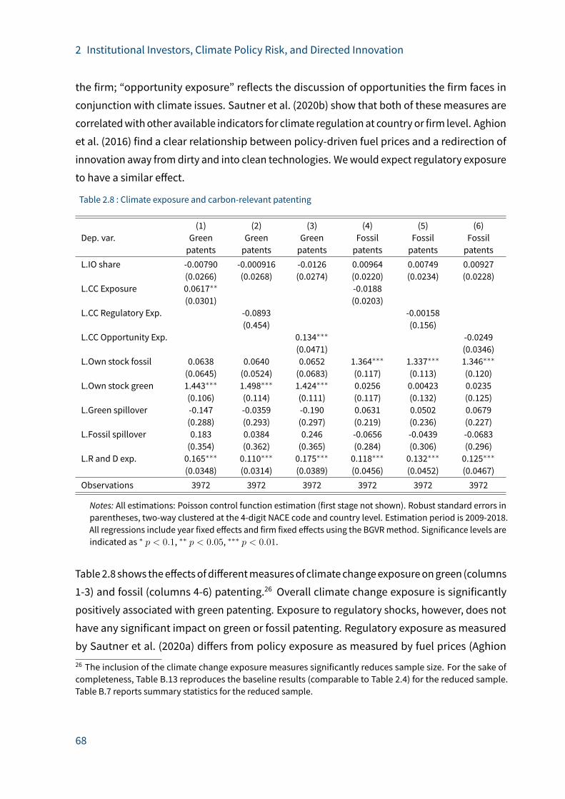
2 Institutional Investors, Climate Policy Risk, and Directed Innovation
the firm; “opportunity exposure” reflects the discussion of opportunities the firm faces in
conjunction with climate issues. Sautner et al. (2020b) show that both of these measures are
correlatedwith other available indicators for climate regulation at country or firm level. Aghion
et al. (2016) find a clear relationship between policy-driven fuel prices and a redirection of
innovation away fromdirty and into clean technologies. Wewould expect regulatory exposure
to have a similar e�ect.
Table 2.8 : Climate exposure and carbon-relevant patenting
(1) (2) (3) (4) (5) (6)Dep. var. Green
patentsGreenpatents
Greenpatents
Fossilpatents
Fossilpatents
Fossilpatents
L.IO share -0.00790 -0.000916 -0.0126 0.00964 0.00749 0.00927(0.0266) (0.0268) (0.0274) (0.0220) (0.0234) (0.0228)
L.CC Exposure 0.0617∗∗ -0.0188(0.0301) (0.0203)
L.CC Regulatory Exp. -0.0893 -0.00158(0.454) (0.156)
L.CC Opportunity Exp. 0.134∗∗∗ -0.0249(0.0471) (0.0346)
L.Own stock fossil 0.0638 0.0640 0.0652 1.364∗∗∗ 1.337∗∗∗ 1.346∗∗∗
(0.0645) (0.0524) (0.0683) (0.117) (0.113) (0.120)L.Own stock green 1.443∗∗∗ 1.498∗∗∗ 1.424∗∗∗ 0.0256 0.00423 0.0235
(0.106) (0.114) (0.111) (0.117) (0.132) (0.125)L.Green spillover -0.147 -0.0359 -0.190 0.0631 0.0502 0.0679
(0.288) (0.293) (0.297) (0.219) (0.236) (0.227)L.Fossil spillover 0.183 0.0384 0.246 -0.0656 -0.0439 -0.0683
(0.354) (0.362) (0.365) (0.284) (0.306) (0.296)L.R and D exp. 0.165∗∗∗ 0.110∗∗∗ 0.175∗∗∗ 0.118∗∗∗ 0.132∗∗∗ 0.125∗∗∗
(0.0348) (0.0314) (0.0389) (0.0456) (0.0452) (0.0467)Observations 3972 3972 3972 3972 3972 3972
Notes: All estimations: Poisson control function estimation (first stage not shown). Robust standard errors inparentheses, two-way clustered at the 4-digit NACE code and country level. Estimation period is 2009-2018.All regressions include year fixed e�ects and firm fixed e�ects using the BGVRmethod. Significance levels areindicated as ∗ p < 0.1, ∗∗ p < 0.05, ∗∗∗ p < 0.01.
Table2.8 shows thee�ectsofdi�erentmeasuresof climatechangeexposureongreen (columns
1-3) and fossil (columns 4-6) patenting.26 Overall climate change exposure is significantly
positively associated with green patenting. Exposure to regulatory shocks, however, does not
have any significant impact on green or fossil patenting. Regulatory exposure as measured
by Sautner et al. (2020a) di�ers from policy exposure as measured by fuel prices (Aghion26 The inclusion of the climate change exposure measures significantly reduces sample size. For the sake ofcompleteness, Table B.13 reproduces the baseline results (comparable to Table 2.4) for the reduced sample.Table B.7 reports summary statistics for the reduced sample.
68
2 Institutional Investors, Climate Policy Risk, and Directed Innovation
et al. 2016) in one key aspect: Fuel prices are measures of existing climate policies. They are
observable, and firms can easily build expectations regarding future fuel prices (at least the tax
component of it) based on past fuel prices. This is what might make lagged fuel prices a good
predictor of green patenting.27 The regulatory climate change exposure measure probably
reflects more long-term expectations voiced by investors. In line with the insignificant results
on institutional owner shares, it seems that the concerns about expected regulation do not
(yet) translate into a change in the direction of innovation within firms.28
Exposure to opportunity shocks, on the other hand, is significantly positively associated with
green patenting. According to these results, a one standard deviation increase in climate
opportunity exposure leads to a staggering 25% increase in green patents (0.134*1.887). As
shown in Table 2.2, the top bigrams for opportunity and overall exposure are very similar,
indicating that the frequency of opportunity-related keywords is driving the results for overall
climate change exposure.
Given the way in which the “climate change opportunity” measure is constructed, it is di�icult
to interpret the e�ect as causal. The question is what “exposure to opportunity shocks” actu-
ally means. Only very few of the underlying bigrams relate to opportunity-creating policies,
which would reflect an exogenous opportunity shock. Looking at the bigrams, it is possi-
ble that investors are makingmanagement aware of green opportunities in a more general
sense, and push for more innovation. It is, however, also likely that managers mention par-
ticular green R&D successes in earnings conference calls – resulting in high “climate change
opportunity” measures –, which are followed by green patent applications in the next year.
Therefore, the results from table 2.8 suggest that “climate change opportunity exposure” is a
good predictor of green patenting activity, but not necessarily reflecting a causal relationship.
Nevertheless, the clear results on climate change opportunity exposure (with the expected
sign) indicate that the patent data exhibit su�icient variation over time to detect e�ects of
firm-specific characteristics related to climate risk and institutional ownership. This is an
indication that the nonsignificant results can be interpreted as “no e�ect”. In this light, it is
interesting that fossil patenting is not a�ected by any climate-related exposure. There is no
27 The fact that tax-driven fuel price changes can lead to larger fuel demand changes is an established result inthe literature on environmental and energy economics, see e.g. Li et al. (2014) and L. W. Davis and Kilian (2011).It is usually attributed to the predictability of the tax component.28 Regressions using the second lag of regulatory exposure yield insignificant coe�icients as well. Results areavailable upon request.
69

2 Institutional Investors, Climate Policy Risk, and Directed Innovation
evidence that green technologies crowd out fossil ones, or that technological risk is addressed
by actively moving out of fossil technologies.
2.6 Conclusion
The tightening of climate policies entails transition risk not only for fossil fuel producers and
emitters, but also for innovators in related technologies: their knowledge is at risk of losing
value due to climate policy. This translates into a risk for investors of the a�ected technology
firms. This paper explores whether institutional investors have recognized this risk, and
whether their engagement directs firms’ innovation into green technologies.
The analysis draws on the growing literature on the role of institutional investors in equity
markets.Via direct conversations and voting in shareholder meetings, large asset managers
and funds can influence the behavior of firms (Appel et al. 2016, 2018; Dimson et al. 2015) and
have been shown to encourage innovation (Aghion et al. 2013; Bushee 1998). The underlying
idea is that many institutional investors have amore long-term perspective than “myopic”
managers who are incentivized by short-term performance goals.
In this paper, I construct a worldwide firm-level panel on patents and institutional ownership.
A classification of patents into green and fossil technology categories is applied to measure
firm-specific technological knowledge and innovation. I then estimate a dynamic patent
count data model building on Aghion et al. (2016), where patenting depends on previous
knowledge, spillovers, R&D e�orts, and the share of institutional ownership. The endogeneity
of institutional ownership is addressed by a control function approach.
I find robust evidence for the positive influence of institutional ownership on overall patenting
activity. However, there is no evidence for any e�ect on fossil or green technologies, not even
for investors with long-term perspective or signatories of the UN Principles for Responsible
Investment (UN PRI). The results also hold when looking specifically at the transport sector,
where technological knowledge likely plays a larger role. These results are in contrast to previ-
ous studies which show a positive relationship between climate policy and green innovation
(Aghion et al. 2016), and between institutional ownership and environmental outcomes (Dyck
et al. 2019; Dimson et al. 2015; Azar et al. 2020). Institutional investors seem to perceive and
address technological risk di�erently from overall environmental or transition risks.
70

2 Institutional Investors, Climate Policy Risk, and Directed Innovation
To find out whether climate-relevant patenting can be explained by firm-specific climate-
related risks, I use a newly developed dataset on firm-level climate exposure (Sautner et al.
2020a). It is basedon firms’ conferencecallswith investorsandmeasures the relative frequency
atwhichclimate-related termsarementioned. I finda significantpositive relationshipbetween
“climate opportunity exposure” and subsequent green variation. I cannot ascertain that this is
a causal e�ect of an exogenous opportunity shock, e.g., green technology support schemes.
What the indicator rather seems to reflect is thatmanagers talk about green innovation activity
that is filed as a patent in the following year.
The results on climate exposure can be used to address another issue. If the insignificant
e�ects I find for institutional ownership just result from a dataset with insu�icient variation,
they do not have any informational value. The climate exposure results show that there is
su�icient statistical power in the data to detect a relationship between green patents and
a variable that is not directly related to innovation. The insignificant e�ect of institutional
ownership on green and fossil innovation can therefore likely be interpreted as a zero e�ect.
It is remarkable that neither institutional ownership, nor firm-specific regulatory or opportu-
nity shocks have any e�ect on fossil patenting. Moving out of fossil technology development
does not (yet) seem an answer to (expected) policies. Possibly, the use of fossil technolo-
gies still generates too much income today to be given up in favor of more future-oriented
technologies; neither investors nor regulation appear to generate su�icient pressure to draw
managers away from their “cash cows”. For the large, publicly listed firms which constitute
my sample, such a turnaroundmay be particularly di�icult.29
One reason for the missing influence of institutional ownership on fossil as well as green
technologies could be related to reputational concerns, or the lack thereof. “ESG risks” are
o�en reputation risks: a firm may be a�ected by negative headlines in case of oil spills or
worker protests, for example. Innovation is less visible. It is possible that investors’ main
concern is about reputational risk, and they are therefore less interested in the direction of
innovation.
29 In the management literature, we can find the idea that established companies focus more on incrementalimprovements, whereas small start-ups create “disruptive innovation” (Christensen et al. 2015). As most greeninnovations can still be regarded asmore “novel” (Dechezleprêtre et al. 2017), a typical strategy for an incumbentfirm would be to continue with their traditional business areas, and to acquire new-technology startups. Infuture research, it would be interesting to see whether an increase in indirect green knowledge acquisition canbe observed in the data, and whether institutional investors support this.
71

2 Institutional Investors, Climate Policy Risk, and Directed Innovation
Policy uncertainty has been shown to reduce innovation (Bhattacharya et al. 2017) and could
be another explanation for the absence of an e�ect of institutional ownership on climate-
relevant patenting. With climate policy uncertainty, investors’ strategy might be to support
innovation in other fields rather than betting on green or fossil technologies. An important
next step in this line of research would be to examine events that reduce policy uncertainty
and the resulting market valuation of green and fossil patenting.
This also points to a related issue: the timing of this analysis. Event studies have shown that
the conclusion of the Paris Agreement changed investors’ expectations regarding climate
policy stringency (Ramelli et al. 2019; Kruse, Mohnen, and Sato 2020). Despite early actions
such as the launch of the UN PRI in 2006, investors may have only started to recognize and
address transition risk more recently. It is possible that too few years have passed since Paris
to detect an e�ect of institutional ownership on the direction of innovation – but repeating
the analysis in a couple of years may provide a di�erent picture.
72
3 Economic E�ects of Regional Energy SystemTransformations: An Application to the BavarianOberland Region
3.1 Introduction
The lack of ambitious responses to climate change from the international community and from
national governmentsmotivates subnational entities to set their owngoals and formulate their
own plans towards the reductions of greenhouse gas emissions in their jurisdictions. From an
economics perspective, national unilateral e�orts (not to mention subnational unilateralism)
are by nomeans the first best response to a global problem. Yet, it is laudable that civil society
comes together and becomes active when they hold the view that they can domore. This is
the case of three districts in the Bavarian Oberland Region, who set themselves the target
to generate as much electricity and heat from renewable sources as they consume by the
year 2035. Since 2014, a research consortium has accompanied the region in identifying its
potential for renewables generation, the degree of acceptability of the di�erent technologies.
Based on this, possible scenarios were formulated for how the transformation path might
look like from now until 2035, and the economic e�ects were quantified.
As it is o�en the case in the policy debate, there is a strong interest from local decisionmakers
in the economic e�ects of the transition to an energy system based on renewable energies.
Thus, the purpose of this study is to analyze the e�ects of the di�erent energy transition
paths on regional value added and on employment, divided into three qualification levels:
low-skilled, medium-skilled, and high-skilled employment. This endeavor poses four main
challenges, whose solutions constitute our contributions to the literature. Our first andmost
important contribution lies in taking into account the scarcity of factors of production and of
financial resources needed to undertake the investments, giving rise to crowding out e�ects.
Related to that, our second contribution involves an extension of Fisher and Marshall (2011)
and Benz et al. (2014) aiming at satisfying the needs of a regional and energy economic
analysis. Third, we base the analysis on an input-output (IO) table where the energy sector is
disaggregated to better account for the specificities of each generation technology and its
73
3 Economic E�ects of Regional Energy System Transformations
interconnections with the rest of the economy. Our fourth contribution consists in taking into
account the fact that the three districts are not economically isolated but interact with each
other and with other regions.
We find that the three districts on the Oberland region benefit from investments towards the
regional energy transition, both in terms of additional value added and employment. Yet, the
positive development comes at the expense of value added and employment in the rest of
the country. Moreover, our analysis shows that medium-skilled employment increases most
across all scenarios. In the light of the current shortage of medium-skilled labor in Germany
(Stippler et al. 2019), this finding represents an alarm signal that calls for integrating labor
market considerations into climate policy strategies.
Previous work on the economic impacts of (renewable) energy policy can be summarized in
three main strands: input-output analysis; ex-post econometric studies, focusing on specific
regions or policies; and more complex models or meta-studies. A number of o�en policy-
commissioned reports use standard input-output analysis, evaluating the additional demand
for products in other sectors due to the construction (and sometimes operation) of renewable
energy facilities (Bickel et al. 2009; Böhmer et al. 2015; Breitschopf et al. 2015; Hirschl et al.
2015; Höher et al. 2015; Lehr et al. 2015, 2011; Lutz et al. 2014; O’Sullivan et al. 2014; Ulrich
and Lehr 2014). Their contribution lies in the construction of a demand vector specific to
the installation (or operation) of di�erent renewable energy technologies. These studies
su�er from three limitations: first, they o�en focus on the construction of renewable energy
plants, therefore concentrating on a one-o� e�ect and neglecting the phase of operations,
in particular their structural e�ect changing the interlinkages and production structure in
the economy. Second, they disregard scarcity aspects: in these models, the demand created
due to renewables expansion is always additional and does not come at the expense of other
economic activities. Third, these studies do not take cross-country interlinkages into account,
ignoring the dimension of internationally traded intermediate and final goods. The same is
true for scholarly articles using an input-output approach, such as Allan et al. (2007) or Lehr
et al. (2008). Heindl and Voigt (2012) represent an exception with respect to the consideration
of crowding out e�ects, yet the interlinkages between countries and regions are not accounted
for in this study.
The second strand of literature concerned with the economic e�ects of renewables expansion
is econometric. For example, in an ex-post econometric exercise controlling for economic
74
3 Economic E�ects of Regional Energy System Transformations
structure and other socio-economic variables, Brown et al. (2012) confirm the positive eco-
nomic and employment e�ects of wind power expansions found in input-output studies.
However, such econometric studies also mostly focus on one-o� e�ects induced by policies
(i.e., the e�ects of constructing or installing power equipment). In a recent analysis, Buchheim
et al. (2020) show that the employment e�ects of increased solar energy installations depend
on the tightness of the labormarket, the e�ects being larger when unemployment is high. The
authors conclude that crowding out is the most plausible explanation for small job e�ects.
This finding in an ex-post study further motivates our consideration of crowding out e�ects in
a forward-looking method.
More complex models such as CGE, PANTA RHEI or E3ME can take crowding-out e�ects as well
as international economic linkages into account (see, e.g., IRENA (2016b), the chapter on net
e�ects in Lehr et al. (2011), or the special issue of the Energy Journal on “Hybrid Modeling
of Energy-Environment Policies”). However, these models rely on a number of assumptions
made “in the background” and are not replicable without access to the computational model.
They are also usually not available at the regional level. Meta-studies have combined results
on job gains in renewable industries and job losses in conventional energy to estimate trade-
o�s (e.g., Meyer and Sommer 2014; Wei et al. 2010). The results of their spreadsheet models
are useful, but not replicable as they rely on the availability of previous studies.
Our approach consists in an IO analysis whichwe extend in several dimensions. The advantage
of IO analysis over othermethods that are commonly used to estimate the economic e�ects of
sectoral developments, like the analysis of value-added chains, lies in the ability to consider
indirect besides direct e�ects on other sectors. That means that if a sector faces an increased
demand for its goods, expanding production does not only increase demand for its direct
inputs, but also for the intermediate inputs used to produce these inputs and so on. This
can only be considered up to a limited extent in an analysis of the value-added chain, as
done in Hirschl et al. (2010, 2015). Thus, to be able to use an IO approach, we construct IO
tables for the three districts in the Bavarian Oberland following the method proposed by
Többen and Kronenberg (2015), based on the German IO table. It allows us to model trade
between the districts as well as with the rest of the country and the rest of the world, which is
important considering that the districts are open economies that interact with other regions.
Thus, the additional demand generated by investments (in renewable energies) is not satisfied
exclusively by the local economy but also by sectors outside of their borders. Ignoring this
would lead to a overestimation of the economic e�ects derived from the investments.
75

3 Economic E�ects of Regional Energy System Transformations
One of the extensions of the traditional IO analysis, which also allows us to rule out further
sources of overestimationof the economic e�ects, is considering scarcity of financial resources
andproduction factors. Wedistinguishbetween investments byprivate households and invest-
ments by institutional investors. Moreover, we di�erentiate between the investment and the
operation phase. In the case of private households, investments (in renewables, renovations
and storage capacity) and the corresponding expenditures during the operation phase crowd
out consumption in the same amount.1 Similarly, investments by institutional investors crowd
out alternative investments. This distinction allows us to take into consideration the di�er-
ent structure of these two final demand components (consumption by private households
and investments by private organizations) and, thus, to explicitly consider the increasingly
important role of private households as investors in the electricity and heating sectors.
For the operations phase, we take into account that the investments increase the capital stock
of the concerned sectors. Assuming full employment of the factors of production and fixed
factor input coe�icients, the increased capital attracts labor from other sectors, reducing
their production. For the analysis of the economic e�ects in the operations phase we further
develop the approaches of Fisher and Marshall (2011) and Benz et al. (2014) to make them
applicable in a context when small regions (which in our case are the three German districts)
are embedded in a systemwith much larger regions such as the rest of the country and the
rest of the world.
An important characteristic of our analysis is that it is made prior to the investments, allowing
to take measures targeted at attenuating possible negative developments. For instance,
the identification of sectors that might be negatively a�ectedmakes it possible to support
them in the appropriate manner before or during the transition. Moreover, identifying the
sectors where labor requirements might increase most strongly allows a proactive approach
to prevent and solve shortage problems.
The contributions of this paper do not only refer to the three districts in the Bavarian Oberland
region. On the contrary, they can be applied to other regions, either at the same or other
levels of regional sub-division, and also to other research and policy questions. Thus, the
methodology, which was further developed to satisfy the needs of a regional analysis, is by no
means exclusive to investments in the energy sector or to the Oberland region. Following the
1 This can be seen as a simple representation of a policy instrument financed by a surcharge on the electricityprice for all consumers, as in the German Renewable Energy Law (EEG).
76
3 Economic E�ects of Regional Energy System Transformations
method described in Section 3.2.2, we can construct IO tables for other subnational regions.
Themethod described in Section 3.2.3 can be applied to analyze the economic e�ects of all
types of investments.
In the following sections, we first outline our approach to produce the multi-regional IO
table, to disaggregate the energy sector, and to assess the e�ects of the energy transition.
Section 3.3 describes the data sources and Section 3.4 presents the e�ects on value added
and employment. Finally, Section 3.5 concludes.
3.2 Methodology
For the analysis of the e�ects of the energy transition we want to consider the impact on the
whole regional economy, taking into account the direct and indirect e�ects. Thus we rely
on input-output analysis for the assessment. This confronts us with three methodological
challenges. First, since subnational tables are not available in Germany, we are required
to produce IO tables for each of the districts and link them to each other and to the tables
for the rest of Germany and the rest of the world. This requires estimating trade between
the three districts of analysis but also of each of the districts with the other two regions.
Second, the energy sector of the multi-regional IO table needs to be disaggregated in such
a way that the di�erent renewable energy technologies and conventional technologies are
considered as individual sectors. This disaggregation is necessary to account for the di�erent
input structures and, therefore, for the specific interconnections of each technology with the
rest of the economy. The third challenge is concerned with the calculation of the economic
e�ects. In this respect, we extend the traditional IO analysis to consider scarcities of financial
resources and production factors and, therefore, to account for the fact that investments in
renewables energies crowd out other investments and production in other sectors. In the
following, we describe howwe address each of these challenges.
3.2.1 Disaggregation of the energy sector
We start by disaggregating the energy sector in both source IO tables: the tables for Germany
and the rest of the world from the World Input-Output Database (WIOD) (Timmer et al. 2015)
and theGerman input-output table (GIOT) fromtheGermanstatistical o�ice. Thus, for instance,
the sector “Electricity, steamandhotwater, production anddistribution services thereof” from
77

3 Economic E�ects of Regional Energy System Transformations
the GIOT is disaggregated into nine subsectors.2 These consists of di�erent renewable and
conventional technologies, transmission and distribution of electricity.3 For disaggregation,
we use the information contained in the IO table for Germany from EXIOBASE 2 (Wood et al.
2015), where the energy sector is disaggregated.4
Table 3.1 : Disaggregation of the intersectoral transactions of the energy sector
Coal Solar Distribution
Sector 1 … Sector j Sector h … Sector H … Sector J
Total
intermediate
Use
Sector 1 z11 … z1j z1h … z1H … z1J z1.
… … … … … … … …
Sector i zi1 … zij zih ziH … …
Coal Sector e ze1 … zej zeh … zeH … zeJ ze.
Electricity
Ele
ctri
city
Solar … …
…
…
…
…
…
… …
Ele
ctri
city
Distribution Sector E zE1 … zEj zEh … zEH … zEJ zE.
… … … … … … … …
Sector I zII … … zIh … zIH … zIJ
Total inputs z.1 z.h … z.H
Ele
ctri
city
To arrive at a matrix like in Table 3.1, we need to calculate the elements in the shaded areas,
where zih represents the input from the non-electricity sector i required in the electricity
subsector h, and zej represents the input from the electricity subsector e required in sector j.
Thus, to calculate zih we scale the input from i required in the (only) electricity sector from
2 For simplicity, in the followingwewill refer to the “Electricity, steamandhotwater, production anddistributionservices thereof” sector as the electricity sector, although it also includes activities di�erent to electricitygeneration.3 For a complete list of the energy sectors see Table C.1 in Appendix C.1 (Sectors 10-18).4 Note that we first need to aggregate the sectors in the EXIOBASE table and in the GIOT to be consistent withour final sector aggregation, described in Table C.1.
78
3 Economic E�ects of Regional Energy System Transformations
the GIOT, zGIOTih :
zih = zGIOTih
zExioih∑h z
Exioih
∀ i 6= e, (3.1)
where∑
h zExioih is the sum of interindustry sales of sector i to all electricity sectors. The
superscriptsGIOT andExio indicate that the variables are obtained from the German IO
table from the German statistical o�ice and from the German EXIOBASE table, respectively.
Accordingly, we calculate zej as
zej = zGIOTej
zExioej∑e z
Exioej
∀ j 6= h. (3.2)
To calculate the entries of the intersectoral transactions between the energy subsectors (i.e.,
in the darker area in Table 3.1) we need to proceed slightly di�erently:
zeh = zGIOTeh
zExioeh∑e
∑h z
Exioeh
, (3.3)
where zeh is the input from the electricity subsector e required in the electricity subsector h.
The remaining components of the IO table for the electricity subsectors, that is, value added,
output, imports of similar final goods, thedi�erent components of final demand (consumption
of private households, consumption of private organizations, consumption of state organiza-
tions, investment and changes in stocks, exports), as well as total final demand are calculated
in a similar manner. For instance, for value added,we, we scalewGIOTh bymultiplying it with
the share ofwExioh in total value added of all electricity subsectors,∑
hwExioh .
3.2.2 Construction of themulti-regional IO table
The goal of the process described in this section is creating amulti-regional IO table consisting
of the IO tables of Miesbach (MB), Bad Tölz-Wolfratshausen (BW), and Weilheim-Schongau
(WS) (together, the Oberland region5), the rest of Germany and the rest of the world. Their
“internal” IO tables are on the main diagonal of the multi-regional matrix; the intermediates
traded interregionally are in the o�-diagonal parts.
5 To be precise, the district Garmisch-Partenkirchen is also part of the administrative Oberland region, but didnot take part in the INOLA research project. For simplicity, we use the terms “Oberland region” and “INOLAregion” interchangeably.
79

3 Economic E�ects of Regional Energy System Transformations
The construction of the multi-regional matrix follows four major steps. First, we construct
regional IO tables by adjusting theGermancoe�icientswith regional output figures and scaling
numbers for final goods use. In a second stepwe employ themodified “cross-hauling adjusted
regionalization method” (CHARM) approach developed by Többen and Kronenberg (2015) to
estimate each district’s sectoral trade flows with the rest of Germany and with the rest of the
world. Applying a simple gravity approach in a third step, wemodel the multi-regional trade
flows: sectoral trade flows between the districts and between each district and non-Oberland
Germany. Finally, using the “proportionality assumption”, we create the multi-regional IO
(MRIO) matrix by combining the data on sectoral trade flows and input coe�icients. So, the
first and the last step are concerned with input-output tables. There we assume that the
production technology in the districts is equal to Germany’s production technology. The inner
two steps are about estimating inner-country trade flows.
Note that the regions we are interested in (the Oberland region) do not sum up to the national
level. We index our districts by b,m, and w and denote the national totals by n. From the
perspective of each district r, the rest of the country is denoted by q, such that, e.g., output is
xi,r + xi,q = xi,n. Similarly, if we look at all three districts together and the respective rest of
the country, this is denoted by roc (the rest of the country, or “non-Oberland region”). The set
G comprises these sub-regions and the rest: g = b,m,w, roc.
Construction of regional IO tables
Gross value added We start with regional data on gross value added, as this measure is the
closest proxy to output that is available from administrative sources. Since regional value
added data is only available at a highly aggregated sectoral level, we disaggregate the data
using employment figures.6 First, we compute preliminary figures for disaggregated value
added,wpi,r, by multiplying with the labor shares of the disaggregated sectors:
wpi,r = wa,r ·Li,rLa,r· wi,n/Li,nwa,n/La,n
, (3.4)
where the subscript a stands for the aggregated sector containing sector i. The third term
on the right hand side (RHS) captures the national productivity di�erences. It is used as a
correction factor to account for potential di�erences in labor productivity across subsectors.
6 Table C.2 provides an overview of the highly aggregated sector level and the comprised sectors.
80

3 Economic E�ects of Regional Energy System Transformations
In a second step, we scale the preliminary values so they match the totals of the aggregated
sectors:
wi,r = wpi,r ·wa,r∑i∈aw
pi,r
. (3.5)
Regional output of non-energy sectors From the sectoral values on regionalw, we com-
pute output by scaling national sectoral output using regional to nationalw shares:
xi,r = xi,n ·wi,rwi,n
, (3.6)
where x denotes output of intermediate and final goods.
The output values of the rest of the country can be calculated as a residual:
xroci = xi,n −∑r
xi,r. (3.7)
Regional output of the energy sectors To take advantage of the fact that we have detailed
information on the energy sectors in the region, we proceed di�erently when regionalizing
these sectors. For each of the electricity and heat generation sectors we scale German output
down to the district level by multiplying it with the ratio of generation (in GWh) in the district,
gi,r to generation in Germany, gi,n per sector:
xi,r = xi,n ·gi,rgi,n
. (3.8)
The scaling factor for regionalization of the “Transmission of electricity” and “Distribution
and trade of electricity” sectors is based on the length of the transmission or the distribution
network located in the region and in the whole of Germany.
Regional input-output matrix For the (technical) regional IOmatrix capturing the use of
intermediates, wemultiply the input-output coe�icients of the German IO table (cij,n) with
the regional output values, assuming identical production technology at the national and
81
3 Economic E�ects of Regional Energy System Transformations
regional level:
zij,r = xj,r · cij,n, (3.9)
where zij,r denotes the input from sector i required in region r’s sector j.
Note that each of the regional matrices constructed in this way is “technical” in the sense that
it doesn’t distinguish between sources of intermediates. It simply states that in a region r and
sector j, a certain amount of inputs from other sectors i is needed to produce this region’s
sectoral output. It does notmake a statement onwhere these inputs come from. The technical
regional input-output matrix derived here is used later on to construct the interregional and
intraregional IO matrices.
Regional domestic final use Final goods use per sector and use item is only available at
the national level.7 We therefore need to scale it using Bavarian data on total final goods use,
and regional data on disposable income in the case of household consumption.
For private household consumption, we start from the national sectoral value and scale it by
Bavarian consumption shares, aswell as regional disposable income in comparison to Bavaria:
dphi,r = dphi,n ·dpbydpn· dirdiby
, (3.10)
with dph denoting consumption (final demand) of private households, dp denoting total private
consumption, di denoting disposable income, and by denoting Bavaria.
For investment and consumption by private and state organizations, we again scale by Bavar-
ian shares following Heindl and Voigt (2012) and then use regional GDP to scale to regional
level:
dki,r = dki,n ·dkbydkn· GDPrGDPby
∀ k 6= cs. (3.11)
7 For simplicity we refer to the di�erent final use items of the IO table as follows:“Final consumption expenditure by households”= private household consumption;“Final consumption expenditure by non-profit organizations serving households”= consumption of privateorganizations;“Final consumption expenditure by government”= consumption of state organizations;“Gross fixed capital formation”= investments;“Changes in inventories and valuables”= changes in stocks.
82
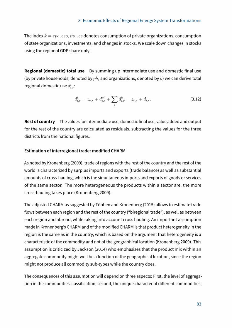
3 Economic E�ects of Regional Energy System Transformations
The index k = cpo, cso, inv, cs denotes consumption of private organizations, consumption
of state organizations, investments, and changes in stocks. We scale down changes in stocks
using the regional GDP share only.
Regional (domestic) total use By summing up intermediate use and domestic final use
(by private households, denoted by ph, and organizations, denoted by k) we can derive total
regional domestic use dti,r:
dti,r = zi·,r + dphi,r +∑k
dki,r = zi·,r + di,r. (3.12)
Restof country The values for intermediate use, domestic final use, value addedandoutput
for the rest of the country are calculated as residuals, subtracting the values for the three
districts from the national figures.
Estimation of interregional trade: modified CHARM
As noted by Kronenberg (2009), trade of regions with the rest of the country and the rest of the
world is characterized by surplus imports and exports (trade balance) as well as substantial
amounts of cross-hauling, which is the simultaneous imports and exports of goods or services
of the same sector. The more heterogeneous the products within a sector are, the more
cross-hauling takes place (Kronenberg 2009).
The adjusted CHARM as suggested by Többen and Kronenberg (2015) allows to estimate trade
flows between each region and the rest of the country (“biregional trade”), as well as between
each region and abroad, while taking into account cross hauling. An important assumption
made in Kronenberg’s CHARM and of themodified CHARM is that product heterogeneity in the
region is the same as in the country, which is based on the argument that heterogeneity is a
characteristic of the commodity and not of the geographical location (Kronenberg 2009). This
assumption is criticized by Jackson (2014) who emphasizes that the product mix within an
aggregate commodity might well be a function of the geographical location, since the region
might not produce all commodity sub-types while the country does.
The consequences of this assumption will depend on three aspects: First, the level of aggrega-
tion in the commodities classification; second, the unique character of di�erent commodities;
83
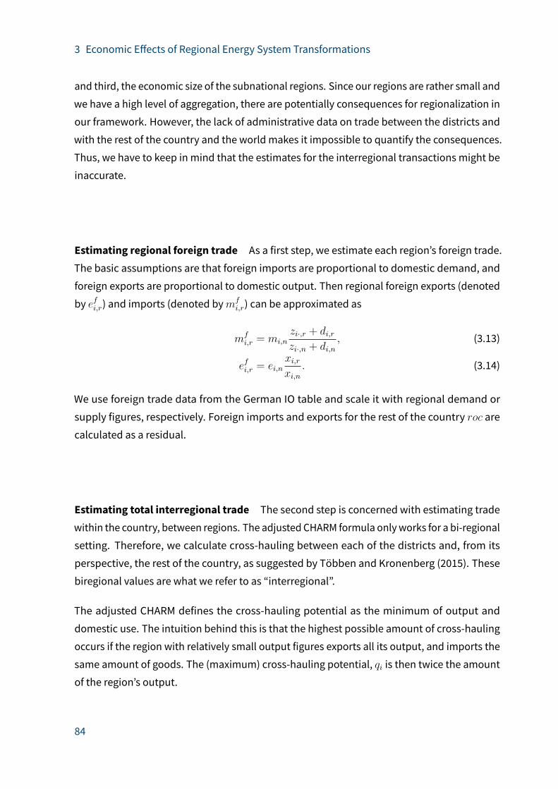
3 Economic E�ects of Regional Energy System Transformations
and third, the economic size of the subnational regions. Since our regions are rather small and
we have a high level of aggregation, there are potentially consequences for regionalization in
our framework. However, the lack of administrative data on trade between the districts and
with the rest of the country and the world makes it impossible to quantify the consequences.
Thus, we have to keep in mind that the estimates for the interregional transactions might be
inaccurate.
Estimating regional foreign trade As a first step, we estimate each region’s foreign trade.
The basic assumptions are that foreign imports are proportional to domestic demand, and
foreign exports are proportional to domestic output. Then regional foreign exports (denoted
by efi,r) and imports (denoted bymfi,r) can be approximated as
mfi,r = mi,n
zi·,r + di,rzi·,n + di,n
, (3.13)
efi,r = ei,nxi,rxi,n
. (3.14)
We use foreign trade data from the German IO table and scale it with regional demand or
supply figures, respectively. Foreign imports and exports for the rest of the country roc are
calculated as a residual.
Estimating total interregional trade The second step is concerned with estimating trade
within the country, between regions. The adjusted CHARM formula onlyworks for a bi-regional
setting. Therefore, we calculate cross-hauling between each of the districts and, from its
perspective, the rest of the country, as suggested by Többen and Kronenberg (2015). These
biregional values are what we refer to as “interregional”.
The adjusted CHARM defines the cross-hauling potential as the minimum of output and
domestic use. The intuition behind this is that the highest possible amount of cross-hauling
occurs if the region with relatively small output figures exports all its output, and imports the
same amount of goods. The (maximum) cross-hauling potential, qi is then twice the amount
of the region’s output.
84
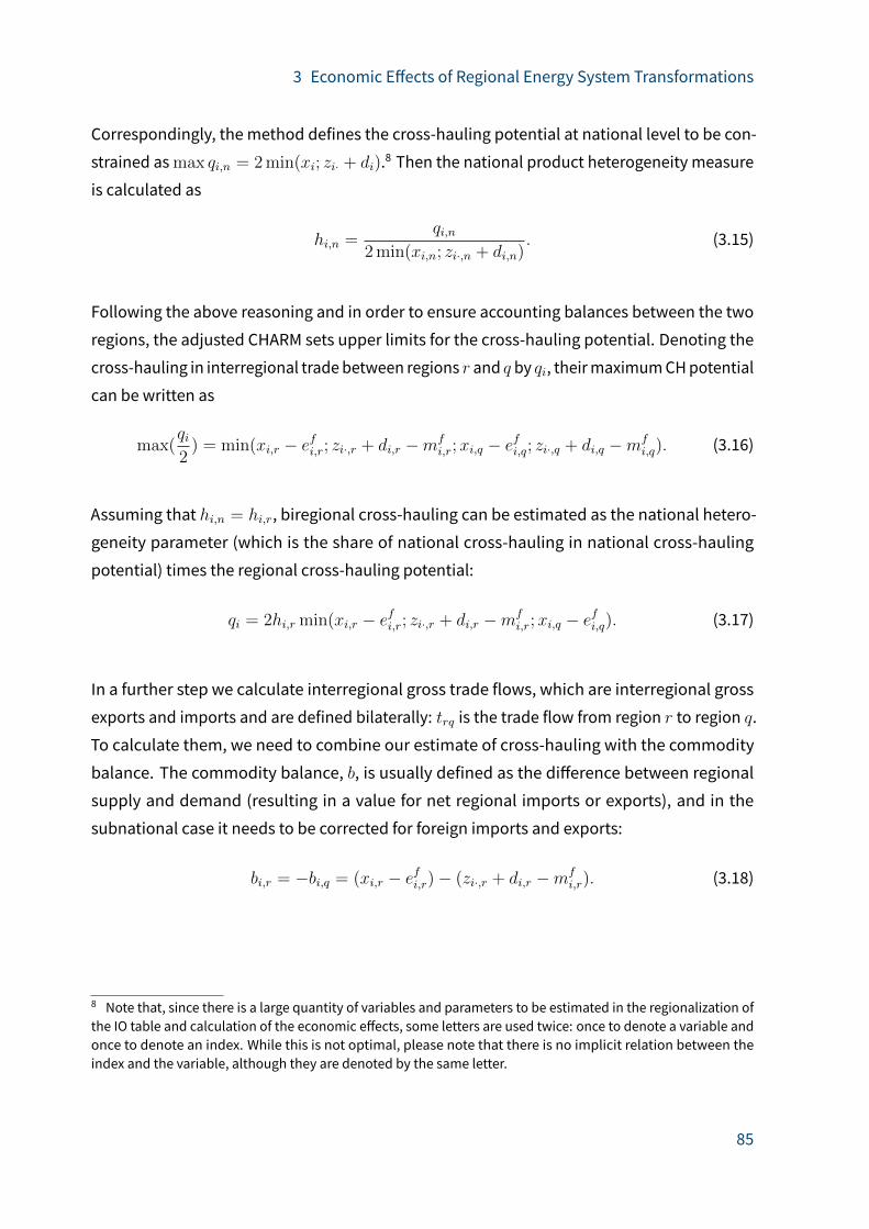
3 Economic E�ects of Regional Energy System Transformations
Correspondingly, the method defines the cross-hauling potential at national level to be con-
strained asmax qi,n = 2 min(xi; zi· + di).8 Then the national product heterogeneity measure
is calculated as
hi,n =qi,n
2 min(xi,n; zi·,n + di,n). (3.15)
Following the above reasoning and in order to ensure accounting balances between the two
regions, the adjusted CHARM sets upper limits for the cross-hauling potential. Denoting the
cross-hauling in interregional tradebetween regions r and q by qi, theirmaximumCHpotential
can be written as
max(qi2
) = min(xi,r − efi,r; zi·,r + di,r −mfi,r;xi,q − e
fi,q; zi·,q + di,q −mf
i,q). (3.16)
Assuming that hi,n = hi,r, biregional cross-hauling can be estimated as the national hetero-
geneity parameter (which is the share of national cross-hauling in national cross-hauling
potential) times the regional cross-hauling potential:
qi = 2hi,r min(xi,r − efi,r; zi·,r + di,r −mfi,r;xi,q − e
fi,q). (3.17)
In a further step we calculate interregional gross trade flows, which are interregional gross
exports and imports and are defined bilaterally: trq is the trade flow from region r to region q.
To calculate them, we need to combine our estimate of cross-hauling with the commodity
balance. The commodity balance, b, is usually defined as the di�erence between regional
supply and demand (resulting in a value for net regional imports or exports), and in the
subnational case it needs to be corrected for foreign imports and exports:
bi,r = −bi,q = (xi,r − efi,r)− (zi·,r + di,r −mfi,r). (3.18)
8 Note that, since there is a large quantity of variables and parameters to be estimated in the regionalization ofthe IO table and calculation of the economic e�ects, some letters are used twice: once to denote a variable andonce to denote an index. While this is not optimal, please note that there is no implicit relation between theindex and the variable, although they are denoted by the same letter.
85
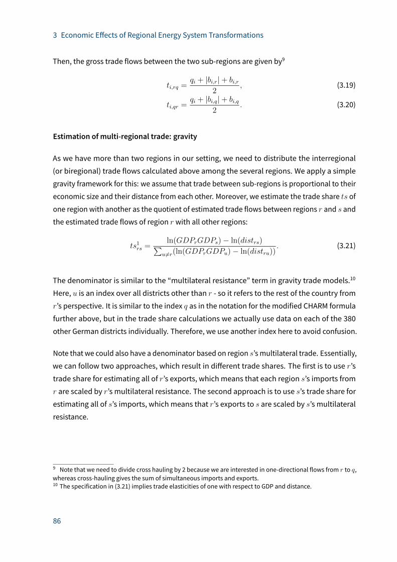
3 Economic E�ects of Regional Energy System Transformations
Then, the gross trade flows between the two sub-regions are given by9
ti,rq =qi + |bi,r|+ bi,r
2, (3.19)
ti,qr =qi + |bi,q|+ bi,q
2. (3.20)
Estimation of multi-regional trade: gravity
As we have more than two regions in our setting, we need to distribute the interregional
(or biregional) trade flows calculated above among the several regions. We apply a simple
gravity framework for this: we assume that trade between sub-regions is proportional to their
economic size and their distance from each other. Moreover, we estimate the trade share ts of
one region with another as the quotient of estimated trade flows between regions r and s and
the estimated trade flows of region r with all other regions:
ts1rs =ln(GDPrGDPs)− ln(distrs)∑
u6=r(ln(GDPrGDPu)− ln(distru)). (3.21)
The denominator is similar to the “multilateral resistance” term in gravity trade models.10
Here, u is an index over all districts other than r - so it refers to the rest of the country from
r’s perspective. It is similar to the index q as in the notation for the modified CHARM formula
further above, but in the trade share calculations we actually use data on each of the 380
other German districts individually. Therefore, we use another index here to avoid confusion.
Note that we could also have a denominator based on region s’s multilateral trade. Essentially,
we can follow two approaches, which result in di�erent trade shares. The first is to use r’s
trade share for estimating all of r’s exports, which means that each region s’s imports from
r are scaled by r’s multilateral resistance. The second approach is to use s’s trade share for
estimating all of s’s imports, which means that r’s exports to s are scaled by s’s multilateral
resistance.
9 Note that we need to divide cross hauling by 2 because we are interested in one-directional flows from r to q,whereas cross-hauling gives the sum of simultaneous imports and exports.10 The specification in (3.21) implies trade elasticities of one with respect to GDP and distance.
86
3 Economic E�ects of Regional Energy System Transformations
Approach 2 reads:
ts2rs =ln(GDPrGDPs)− ln(distrs)∑
u6=s(ln(GDPsGDPu)− ln(distsu)). (3.22)
Combining the multi-regional trade share with interregional trade flows gives the multi-
regional trade flows (shown here according to approach 1):
t1i,rs = ti,rq · ts1rs. (3.23)
Trade between each district and the non-INOLA region is calculated as a residual. So, for
instance for district b
tb,roc = tbq − tbm − tbw, (3.24)
where q denotes the rest of the country from the perspective of the exporting district, andm
andw denote the other two Oberland districts.
Since both approaches for the calculation of the districts’ trade flows lead to di�erent esti-
mates, we chose to combine the two approaches. To guarantee that the calculation for the
rest of the country in (3.24) does not deliver negative values, we always use the smaller of the
two:
ti,rs = min(t1i,rs; t2i,rs). (3.25)
Construction of themulti-regional IOmatrix
Imported intermediates: proportionality assumption To construct theMRIOmatrix from
the technical IOmatrix and themulti-regional trade flows, we use the proportionality assump-
tion also used by Benz et al. (2014) among others. According to this assumptions “an industry
uses an import of a particular product in proportion to its total use of that product” (OECD
2002, p. 12). For example, if the motor vehicles industry in region A uses steel in production
and 10% of all steel is imported from a particular region B, then 10% of the steel used by the
motor vehicles industry in region A is imported from region B.
87
3 Economic E�ects of Regional Energy System Transformations
So the intermediate inputs used by region r’s sector i from region s’s sector j read as
zij,sr = zij,rtj,srdtj,r
, (3.26)
where dtj,r denotes total use of product j in region r. In a similar manner, we calculate the
intermediate inputs used by region r’s sector i from sector j of the rest of the world (ROW),
using the foreign importsmfi,r calculated above and the proportionality assumption, and
denote them zrowij,r .
Intersectoral transactions within each district We then calculate the within-district IO
matrix as the residual of the “technical” matrix calculated above, and all imported intermedi-
ates from the other districts, the rest of the country and the rest of the world
zij,rr = zij,r −∑s6=r
zij,s − zij,rowr. (3.27)
Linking the regional and German tables to the rest of the world Having the MRIO table
for the districts and the rest of the country, we proceed to link it to the rest of the world.
We aggregate the individual countries of the WIOD table (except Germany) to form the ROW
region and the sectors to match the sectors of the IO tables for the districts. Aggregated WIOD
tables are taken as the base table. We then disaggregate the intersectoral transaction within
Germany from the WIOD table, zWIODij,n using origin-destination shares that can be calculated
from the MRIO table generated using the methodology described above:
zij,rs = zWIODij,n
zGIOTij,rs∑r
∑s z
GIOTij
, (3.28)
where the superscript GIOT denotes the variables that were calculated above using the
German IO table from the German statistical o�ice. The intersectoral transactions between
German sectors and ROW’s sectors are regionalized in proportion to output, that is: zij,rrow =
zWIODij,nrow
xGIOTi,r
xGIOTi,n
.
88
3 Economic E�ects of Regional Energy System Transformations
Factors of production
Starting from the production factor figures for Germany, we scale down the respective factor
to the district level using the sectoral factor coe�icients for Germany and sectoral output for
the districts. For instance, we computeKir, the capital stock in region r’s sector i, as
Kir = Kinxi,rxi,n
, (3.29)
whereKin denotes the sectoral capital stock for the whole of Germany. The factors of produc-
tion for the rest of the world are calculated in a similar way.
3.2.3 Economic e�ects: extended IO analysis
Being placed in an IO framework, we implicitly assume a Leontief production function with
fixed input coe�icients and constant returns to scale. Furthermore, although the period of
analysis is relatively long (from 2015 to 2035), we also need to make the assumption that the
input coe�icients and factors coe�icients will stay the same throughout the period of analysis,
that is, the production technology of the economy will remain unchanged. This assumption
becomes more realistic for other possible applications with shorter periods of analysis.
For the assessment, we consider both the one-o� e�ects of the investment (or construction)
phase aswell as the e�ects of the operations phase. Importantly, we take into account scarcity
of financial resources and of the factors of production, thus in the investment and in the
operation phase crowding out of other activities occurs. Specifically, investments in the
energy transition crowd out other investments by companies or consumption by private
households. Here we assume that financial resources do not only come from the region where
investments take place but also from other regions. The rationale behind this assumption
is that investments in the energy transition are typically financed by national climate policy
instruments that redistribute funds from the whole of the country to the actual investment
location.11 Similarly, in the operations phase factors of production that could be employed
otherwise, are used in the operation andmaintenance of renewables, reducing their activity
(and therefore output) in other sectors.
11 An example for such a redistribution mechanism is the German EEG which finances the investments via asurcharge on the electricity price paid by all consumers (with some exceptions). In the case where policies arefinanced by the national public budget, redistribution occurs through the tax system.
89

3 Economic E�ects of Regional Energy System Transformations
The next subsections describe our methodology. First, we introduce the general method
to compute the amount of output necessary to meet the additional investment demand
generated by the energy transition. We then present the method to consider scarcities in the
investment phase and the operation phase. Finally, we show howwe calculate the e�ects on
value added and employment, starting from the additional output figures.
Additional output
The starting point of our analysis are the future investments in renewable energies for elec-
tricity and heat generation, energy e�iciency measures and electricity storage appliances.12
We denote these by f , which is aN × 1 column vector, whereN is the total number of sectors
per region. The vector f describes how total demand for investment goods is composed of
investment goods from other specific sectors, thus it breaks down the overall investment
in region r into the components needed from each sector i. Note that this vector does not
provide information on the geographical origin of the components yet, thus we use the intra-
sectoral transactions in intermediates from theMRIO table as a proxy to distribute the sectoral
investment demand among the regions and obtain the additional investment demand:
∆dinv = Uf . (3.30)
where dinv is anNR×1 column vector, andR is the total number of regions.U is aNR×NRmatrix whose elements, uij,rs, describe the share of zij,rs (i.e., of inputs from region r’s sector
i used in regions s’s sector j), in the intrasectoral transactions:
uij,rs =zij,rs∑R
r=1
∑Rs=1 zij,rs
∀ i = 1, . . . , N and j = i. (3.31)
12 For simplicity, in the following the expression investment in renewables will also mean energy e�iciencymeasures and the deployment of storage capacity.
90

3 Economic E�ects of Regional Energy System Transformations
Following classical IO analysis, the amount of output of final goods and intermediates,∆x,
that is necessary to satisfy the additional investment demand can be computed as follows:
∆x = (I− L)−1∆dinv, (3.32)
where I is the unitymatrix andL is thematrix of fixed input coe�icients, which shows thedirect
use of intermediates per unit of output. Leontief’s inverse, (I− L)−1, is the matrix to which
the infinite series of powers ofL converges. Accordingly, it accounts for the fact that, besides
the directly used intermediates, output production also uses indirectly the intermediates
used for production of the direct intermediates and so on. Thus, Leontief’s inverse indicates
the level of output needed to satisfy a unit vector of final demand a�er infinite rounds of this
process.
To this point we have not considered any scarcity e�ects and have assumed that additional
resources and factors of production are readily available and enter the system in an unlimited
manner. However, it is more reasonable to assume that investments in renewables crowd out
other types of demand, e.g., alternative investment or consumption by private households.
Moreover, factors of production are not unlimited in stock and waiting to be employed. To
consider scarcity e�ects we follow two di�erent approaches depending on the actors under-
taking the investment: private households or institutional investors. Moreover, we distinguish
between the investment phase and the operation phase.
Considering scarcity in the investment phase Crowding out in the investment phase for
both types of investors follows a similar principle: investments in renewables crowds out an
alternative average investment (alternative average consumption) in the same amount as the
total investment in renewables. Thus, the calculation of additional output, net of crowding
out reads:
∆xinv,net = (I− L)−1(∆dinv,ii + ∆dinv,ph −∆dinvco −∆dphco), (3.33)
where∆dinv,ii and∆dinv,ph denote the additional investment demand generated by institu-
tional investors and by private households, respectively.∆dinvco is a vector of crowded out
investment demand and∆dphco is a vector of crowd out consumption by private households.
91
3 Economic E�ects of Regional Energy System Transformations
The elements of∆dinvco are defined as
∆dinvcoi,r =dinvi,r∑i,r d
invi,r
∑i,r
∆dinv,iii,r . (3.34)
The fraction on the right hand side of (3.34) describes the proportional distribution of an
average investment among sectors and regions.13 In other words, it describes howmany cents
out of each Euro invested in any of the regions appear as investment demand in a specific
regional sector. The last term on the right hand side is the sum of the investments.∆dphco
is similarly defined, yet in this case an average consumption vector is multiplied with the
additional investment demand generated by private households.
Considering scarcity in the operation phase To consider crowding out in the operations
phase, we apply and modify the approach introduced by Fisher and Marshall (2011) to an
energy economic analysis, and extend it to suit the requirements of an analysis of small regions
embedded in an international IO table.
Before turning to the formal representation, consider first the intuition behind our approach,
which is based on Rybczynski e�ects (Rybczynski 1955) well-known in the trade literature
(see Feenstra 2004). By investing in renewables, the capital stock of each renewables sector
increases by the amount of the respective investment. Assuming that there are no changes in
technology, the capital stock increase attracts into the renewables sectors the amount of labor
that is necessary to use the new capital stock in the production process. Assuming scarcity in
the factors of production, which is a sensible assumption considering the current situation
on the German labor market, labor is necessarily attracted from other sectors of the same
or of other regions. Thus, output in these sectors decreases. This is, of course, a simplified
representation of the whole process, since actually the adjustment consists of infinite rounds
of intermediate input sectors.
Formally, we assume the Leontief production function to be transregional as in Benz et al.
(2014). That means that production of final goods in one region potentially uses factor inputs
from all other regions by using intermediates from the other regions. The production function
13 Recall that dinvi,r is investment demand and is readily available for the IO tables.
92
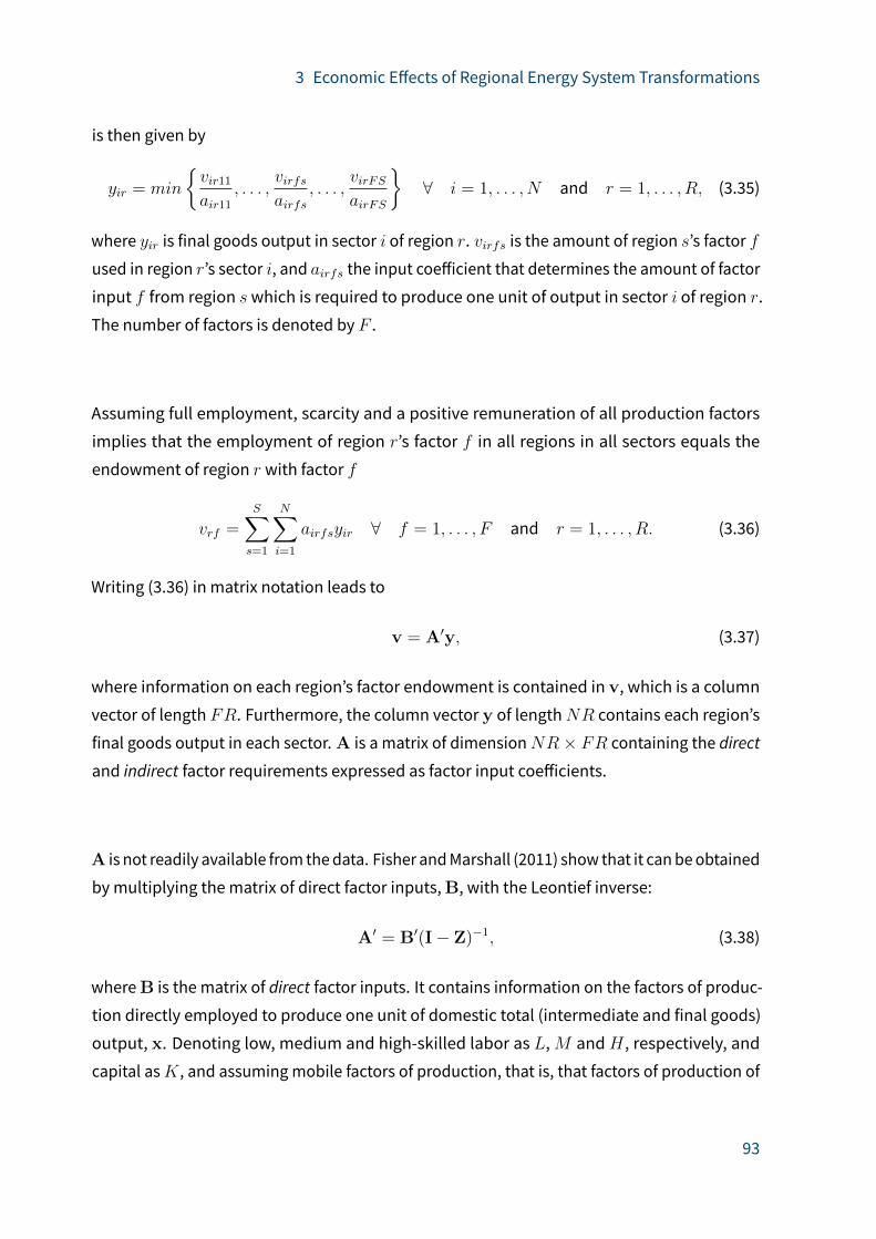
3 Economic E�ects of Regional Energy System Transformations
is then given by
yir = min
{vir11air11
, . . . ,virfsairfs
, . . . ,virFSairFS
}∀ i = 1, . . . , N and r = 1, . . . , R, (3.35)
where yir is final goods output in sector i of region r. virfs is the amount of region s’s factor f
used in region r’s sector i, and airfs the input coe�icient that determines the amount of factor
input f from region swhich is required to produce one unit of output in sector i of region r.
The number of factors is denoted by F .
Assuming full employment, scarcity and a positive remuneration of all production factors
implies that the employment of region r’s factor f in all regions in all sectors equals the
endowment of region r with factor f
vrf =S∑s=1
N∑i=1
airfsyir ∀ f = 1, . . . , F and r = 1, . . . , R. (3.36)
Writing (3.36) in matrix notation leads to
v = A′y, (3.37)
where information on each region’s factor endowment is contained in v, which is a column
vector of length FR. Furthermore, the column vector y of lengthNR contains each region’s
final goods output in each sector.A is a matrix of dimensionNR× FR containing the directand indirect factor requirements expressed as factor input coe�icients.
A is not readily available from thedata. Fisher andMarshall (2011) show that it canbeobtained
by multiplying the matrix of direct factor inputs,B, with the Leontief inverse:
A′ = B′(I− Z)−1, (3.38)
whereB is the matrix of direct factor inputs. It contains information on the factors of produc-
tion directly employed to produce one unit of domestic total (intermediate and final goods)
output, x. Denoting low, medium and high-skilled labor as L,M andH , respectively, and
capital asK, and assuming mobile factors of production, that is, that factors of production of
93
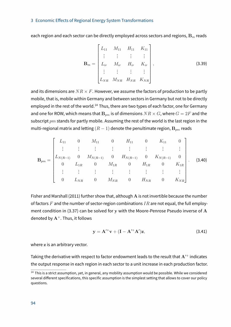
3 Economic E�ects of Regional Energy System Transformations
each region and each sector can be directly employed across sectors and regions,Bm reads
Bm =
L11 M11 H11 K11
......
......
Lir Mir Hir Kir
......
......
LNR MNR HNR KNR
, (3.39)
and its dimensions areNR× F . However, we assume the factors of production to be partlymobile, that is, mobile within Germany and between sectors in Germany but not to be directly
employed in the rest of the world.14 Thus, there are two types of each factor, one for Germany
and one for ROW, whichmeans thatBpm is of dimensionsNR×G, whereG = 2F and the
subscript pm stands for partly mobile. Assuming the rest of the world is the last region in the
multi-regional matrix and letting (R− 1) denote the penultimate region,Bpm reads
Bpm =
L11 0 M11 0 H11 0 K11 0...
......
......
......
...
LN(R−1) 0 MN(R−1) 0 HN(R−1) 0 KN(R−1) 0
0 L1R 0 M1R 0 H1R 0 K1R
......
......
......
......
0 LNR 0 MNR 0 HNR 0 KNR
. (3.40)
Fisher andMarshall (2011) further show that, althoughA is not invertible because the number
of factors F and the number of sector-region combinations IR are not equal, the full employ-
ment condition in (3.37) can be solved for y with the Moore-Penrose Pseudo inverse ofA
denoted byA+. Thus, it follows
y = A′+v + (I−A′+A′)z, (3.41)
where z is an arbitrary vector.
Taking the derivative with respect to factor endowment leads to the result thatA′+ indicates
the output response in each region in each sector to a unit increase in each production factor.
14 This is a strict assumption, yet, in general, any mobility assumption would be possible. While we consideredseveral di�erent specifications, this specific assumption is the simplest setting that allows to cover our policyquestions.
94
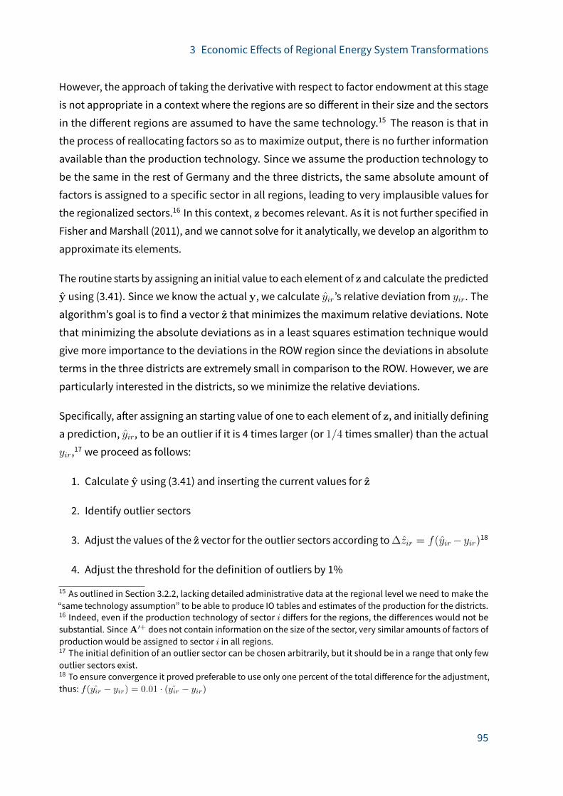
3 Economic E�ects of Regional Energy System Transformations
However, the approach of taking the derivative with respect to factor endowment at this stage
is not appropriate in a context where the regions are so di�erent in their size and the sectors
in the di�erent regions are assumed to have the same technology.15 The reason is that in
the process of reallocating factors so as to maximize output, there is no further information
available than the production technology. Since we assume the production technology to
be the same in the rest of Germany and the three districts, the same absolute amount of
factors is assigned to a specific sector in all regions, leading to very implausible values for
the regionalized sectors.16 In this context, z becomes relevant. As it is not further specified in
Fisher and Marshall (2011), and we cannot solve for it analytically, we develop an algorithm to
approximate its elements.
The routine starts by assigning an initial value to each element of z and calculate the predicted
y using (3.41). Since we know the actual y, we calculate yir’s relative deviation from yir. The
algorithm’s goal is to find a vector z that minimizes themaximum relative deviations. Note
that minimizing the absolute deviations as in a least squares estimation technique would
give more importance to the deviations in the ROW region since the deviations in absolute
terms in the three districts are extremely small in comparison to the ROW. However, we are
particularly interested in the districts, so weminimize the relative deviations.
Specifically, a�er assigning an starting value of one to each element of z, and initially defining
a prediction, yir, to be an outlier if it is 4 times larger (or 1/4 times smaller) than the actual
yir,17 we proceed as follows:
1. Calculate y using (3.41) and inserting the current values for z
2. Identify outlier sectors
3. Adjust the values of the z vector for the outlier sectors according to∆zir = f(yir− yir)18
4. Adjust the threshold for the definition of outliers by 1%
15 As outlined in Section 3.2.2, lacking detailed administrative data at the regional level we need tomake the“same technology assumption” to be able to produce IO tables and estimates of the production for the districts.16 Indeed, even if the production technology of sector i di�ers for the regions, the di�erences would not besubstantial. SinceA′+ does not contain information on the size of the sector, very similar amounts of factors ofproduction would be assigned to sector i in all regions.17 The initial definition of an outlier sector can be chosen arbitrarily, but it should be in a range that only fewoutlier sectors exist.18 To ensure convergence it proved preferable to use only one percent of the total di�erence for the adjustment,thus: f(yir − yir) = 0.01 · (yir − yir)
95

3 Economic E�ects of Regional Energy System Transformations
5. Repeat steps 1 to 4 until there are no more improvements in the relative deviations
within a chosen limit of iterations (1 million in our case).
We can then insert the estimated z in (3.41). We extend the right term of the right hand side
by v+v = 1 to obtain
y = (A′+ + (I−A′+A′)zv+)v. (3.42)
This last transformation allows us to determine how sectoral final goods output, y, reacts to
changes in the factors of production. We define the outer parentheses on the right hand side
of (3.42) as
Λ = A′+ + (I−A′+A′)zv+, (3.43)
whereΛ is a matrix whose columns indicate the response in final goods output in each sector
in each region to a unit increase in each factor of production. We extract the columns ofΛ
to have eight single column vectors, one for each factor of production. So, for instance, the
vector containing the e�ect of a unit increase in the capital stock in Germany on output is
denoted as λKG.
Having all the elements to compute the change in output of intermediate and final goods,
we can now outline the procedure. First, we calculate the initial change in output without
considering scarcities as follows:
∆xop,p = (I− L)−1∆dK, (3.44)
where∆dK is a vector of the changes in final demand, whose elements are calculated by
multiplying∆Kir and the fraction of final demand per capital stock, dirKir. Furthermore, we
assume that∆Kir is equal to the investment in each type of renewables.
The preliminary changes in x require changes in the employment of production factors. We
denote these preliminary changes ∆Kop,pir , ∆Lop,pir , ∆M op,p
ir , ∆Hop,pir and compute them as
follows:
∆Hop,pir = ∆xop,pir
Hir
xir, (3.45)
96
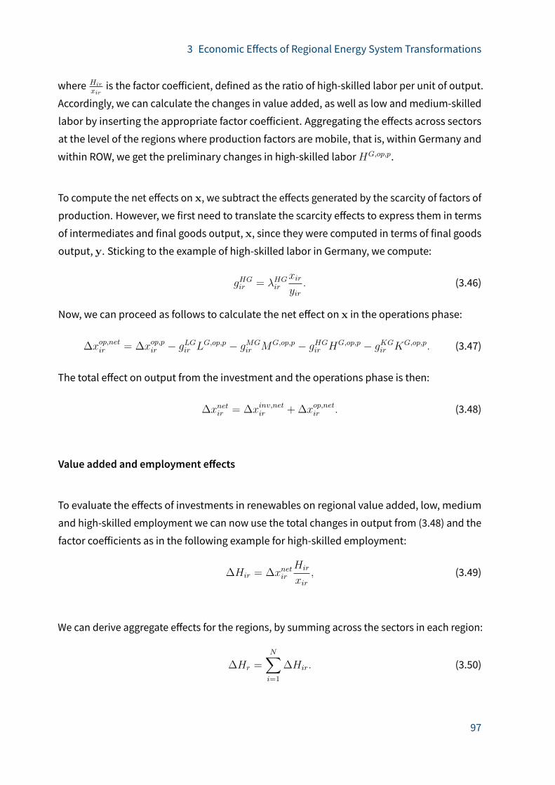
3 Economic E�ects of Regional Energy System Transformations
where Hir
xiris the factor coe�icient, defined as the ratio of high-skilled labor per unit of output.
Accordingly, we can calculate the changes in value added, as well as low andmedium-skilled
labor by inserting the appropriate factor coe�icient. Aggregating the e�ects across sectors
at the level of the regions where production factors are mobile, that is, within Germany and
within ROW, we get the preliminary changes in high-skilled laborHG,op,p.
To compute the net e�ects on x, we subtract the e�ects generated by the scarcity of factors of
production. However, we first need to translate the scarcity e�ects to express them in terms
of intermediates and final goods output, x, since they were computed in terms of final goods
output, y. Sticking to the example of high-skilled labor in Germany, we compute:
gHGir = λHGirxiryir. (3.46)
Now, we can proceed as follows to calculate the net e�ect on x in the operations phase:
∆xop,netir = ∆xop,pir − gLGir LG,op,p − gMGir MG,op,p − gHGir HG,op,p − gKGir KG,op,p. (3.47)
The total e�ect on output from the investment and the operations phase is then:
∆xnetir = ∆xinv,netir + ∆xop,netir . (3.48)
Value added and employment e�ects
To evaluate the e�ects of investments in renewables on regional value added, low, medium
and high-skilled employment we can now use the total changes in output from (3.48) and the
factor coe�icients as in the following example for high-skilled employment:
∆Hir = ∆xnetir
Hir
xir, (3.49)
We can derive aggregate e�ects for the regions, by summing across the sectors in each region:
∆Hr =N∑i=1
∆Hir. (3.50)
97
3 Economic E�ects of Regional Energy System Transformations
Similarly, we can aggregate the e�ects to present results for the single sectors, across regions:
∆Hi =R∑r=1
∆Hir, (3.51)
or aggregate to consider only the three districts.
3.3 Data
3.3.1 Input-output table
The IO tables on which the analysis is based are the German IO table of inland production
and imports for the year 2014 and the 2014 World IO Table fromWIOD (Timmer et al. 2015).
For disaggregation of the energy sector we use Exiobase 2 (Wood et al. 2015), which is, to our
knowledge, the only table where the energy sector is disaggregated into several electricity
production technologies, electricity transmission, electricity distribution, heat production,
and gas distribution.
3.3.2 Regional data
From the Regional Accounts database of the federal and regional statistical o�ices we obtain
data for thedistricts’ GDP, aggregated gross value addeddata anddisposable incomeof private
households for the districts. GDP, government consumption, gross investments in equipment
and buildings and private consumption for Germany and Bavaria are also obtained from this
database. Employment statistics by sector both for Germany and the districts come from the
federal employment statistics o�ice.
Electricity and heat consumption, as well as data on electricity generation in the three districts
was obtained from Reinhardt et al. (2017). Updated information was generously provided by
the authors. Data on the length of electricity transmission lines in the districts were obtained
from the Bavarian State Ministry of Economics and Energy (StMWi 2018). Data on electricity
and heat generation by energy source in Germany comes from IEA (2017).
98
3 Economic E�ects of Regional Energy System Transformations
3.3.3 Factors of production
The three categories of labor input (low-, medium-and high-skilled) for Germany and the ROW
are also from Exiobase 2 (Wood et al. 2015). Data for capital stocks for Germany had to be
derived from various sources. For standard NACE 2-digit sectors, capital stocks are available
from Eurostat (2016a) (total non-financial fixed assets, gross at replacement costs). For the
energy subsectors, capital stocks were disaggregatedmanually. The general approach was
to calculate the capital stock in each subsector from existing data on installed capacity and
the current costs of building such capacity, such as to approximate replacement costs. In a
second step, the results were scaled to the total capital stock of the energy sector available
from Eurostat (2016a). Details on the data sources can be found in Appendix C.2.
3.3.4 Future renewables deployment and investments
Future deployment of renewables for electricity and heat generation, energy e�iciency mea-
sures and electricity storage in each of the three districts were obtained from the simulations
done in the framework of the project by two Geography Departments of LMUMunich. Thus,
the deployment figures constitute an exogenous input in the present study. The simulations
are based on the natural potential for renewable energy generation in the region, the available
land use restrictions (e.g., due to conservation areas), the preferences of the population re-
garding technology types and installations’ size, and the profitability of themeasures, besides
the usually considered factors like interest rates and energy prices.
The scenarios are constructed along twodimensions: one describing the overall economic and
social setting, andanotheroutliningpossibledeploymentpaths. The first dimensionconsiders,
on the one hand, a business-as-usual (BAU) scenario and, on the other hand, a scenario
with a trend towards a more sustainable economy and society (GREEN). The deployment
paths di�erentiate between focusing primarily on small scale installations or on large scale
installations of renewable energies. Combining both dimensions leads to four scenarios: BAU
SMALL, BAU LARGE, GREEN SMALL, and GREEN LARGE.19 From the simulations we obtain the
annual average sum of renovation expenditures per district and information on the capacity
(in kWp) installed per technology type and year from 2015 to 2035. In our analysis, we consider
the average installed capacity per year.19 For more information on the simulations see Danner et al. (2019). Table C.3 in Appendix C.3 provides anoverview of the scenarios. For a more detailed information of the scenario construction process, see Musch andStreit (2017).
99
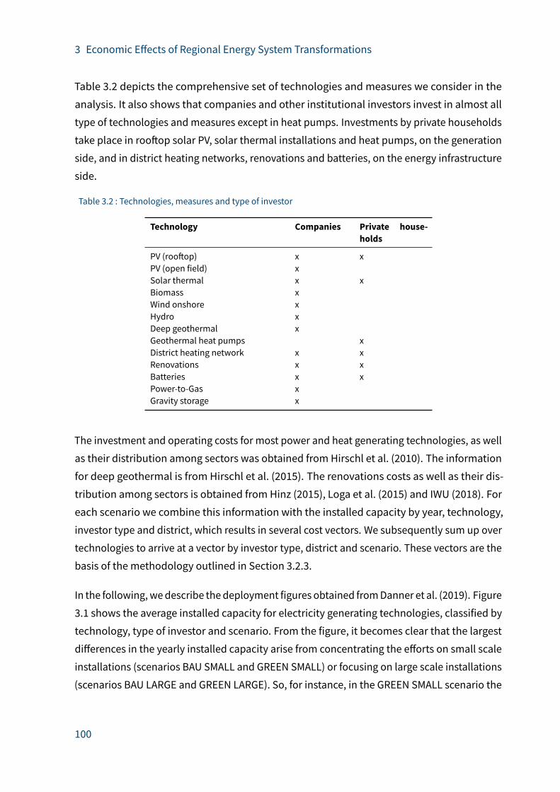
3 Economic E�ects of Regional Energy System Transformations
Table 3.2 depicts the comprehensive set of technologies and measures we consider in the
analysis. It also shows that companies and other institutional investors invest in almost all
type of technologies andmeasures except in heat pumps. Investments by private households
take place in roo�op solar PV, solar thermal installations and heat pumps, on the generation
side, and in district heating networks, renovations and batteries, on the energy infrastructure
side.
Table 3.2 : Technologies, measures and type of investor
Technology Companies Private house-holds
PV (roo�op) x xPV (open field) xSolar thermal x xBiomass xWind onshore xHydro xDeep geothermal xGeothermal heat pumps xDistrict heating network x xRenovations x xBatteries x xPower-to-Gas xGravity storage x
The investment and operating costs for most power and heat generating technologies, as well
as their distribution among sectors was obtained from Hirschl et al. (2010). The information
for deep geothermal is from Hirschl et al. (2015). The renovations costs as well as their dis-
tribution among sectors is obtained from Hinz (2015), Loga et al. (2015) and IWU (2018). For
each scenario we combine this information with the installed capacity by year, technology,
investor type and district, which results in several cost vectors. We subsequently sum up over
technologies to arrive at a vector by investor type, district and scenario. These vectors are the
basis of the methodology outlined in Section 3.2.3.
In the following, wedescribe thedeployment figures obtained fromDanner et al. (2019). Figure
3.1 shows the average installed capacity for electricity generating technologies, classified by
technology, type of investor and scenario. From the figure, it becomes clear that the largest
di�erences in the yearly installed capacity arise from concentrating the e�orts on small scale
installations (scenarios BAU SMALL and GREEN SMALL) or focusing on large scale installations
(scenarios BAU LARGE and GREEN LARGE). So, for instance, in the GREEN SMALL scenario the
100

3 Economic E�ects of Regional Energy System Transformations
Figure 3.1 : Installed capacity by scenario, yearly average
02
46
02
46
PV (rooft
op)
PV (rooft
op)
PV (ope
n fiel
d)
Deep ge
otherm
alHyd
ro
Wind
onsho
re
PV (rooft
op)
PV (rooft
op)
PV (ope
n fiel
d)
Deep ge
otherm
alHyd
ro
Wind
onsho
re
BAU LARGE BAU SMALL
GREEN LARGE GREEN SMALL
Households Institutional Investors
Yea
rly a
vera
ge in
stal
led
capa
city
(MW
)
Electricity generating technologies
average installed capacity of roo�op solar by households is, with 6 MW, twice as large than in
the GREEN LARGE scenario. The contrary and with even more pronounced di�erences, occurs
for wind installations, where the average installed capacity in the GREEN LARGE is 6MW versus
1.2 under the GREEN SMALL scenario. Figure C.1 in the Appendix shows a similar pattern for
heat generating technologies.
Expressing these figures in relation to the number of inhabitants allows a comparison to
current deployment in the whole of Bavaria. We see that for the GREEN LARGE scenario, the
yearly PV and wind installations are equivalent to 25.7 kW per 1,000 inhabitants and 18.5 kW
per 1,000 inhabitants, respectively. The newly installed capacity in kW per 1,000 inhabitants
in Bavaria for the year 2017 (2018) was 50.9 (31.3) for PV and 24.2 (17) for wind (Agentur für
Erneuerbare Energien 2019). Thus, putting the regional deployment figures into context shows
that, although the regional energy transition in the Bavarian Oberland requires an important
deployment of renewable technologies, it does not require an unrealistic development. Yet,
it is important to mention that these deployment scenarios would not achieve a complete
coverage of the energy demand by renewables by 2035, but would bring the coverage rate in
electricity from 38% in 2015 to 51-62% in 2035. For heating, the coverage rate would increase
from 26% in 2015 to 62-66% in 2035. Although the natural and technical potential would allow
the region tomeet its target by 2035, in the deployment simulations an annual technology
specific “administrative installation cap” was set. The main rationale behind this cap was
101
3 Economic E�ects of Regional Energy System Transformations
to account for the observed limited capacity of the public administration when it comes to
granting the necessary licenses for the installation of renewable energies.
3.4 Results
In this section we present the results obtained by applying the methodology outlined in
Section 3.2 to investigate the economic e�ects of a future energy transition in the Bavarian
Oberland region. We start by presenting aggregated e�ects for the whole region and then
dig deeper and show value added and employment e�ects for the individual districts and for
individual sectors.
3.4.1 E�ects on value added
Investments in renewables generate an aggregated regional value added ranging from 252 to
325Million EUR, depending on the scenario, as shown in Figure 3.2. Considering that the value
added in 2014 amounted to 9.5 Billion EUR, the presented figures translate to an increase in
value added of between 2.6% and 3.4%. In Figure 3.3 we see that all three districts benefit to
a similar extent from RES investments in absolute terms. The overall e�ects for the whole of
Germany (that is, including the Oberland region) are also positive, yet the rest of the country
su�ers from the crowding out of alternative investments and consumption, and from the
Oberland region attracting factors of production which are then missing for production in the
rest of Germany. The reason for the overall e�ects for Germany to be positive is that we allow
for financial resources to be attracted from the rest of the world when considering crowding
out e�ects in the investment phase. This approach leads to a lower investment crowding out
in Germany than if we had restricted financial resources in the investment phase to come only
from Germany.
Looking at the sectoral e�ects in Figure 3.4, which shows exemplarily the results for the
GREEN LARGE scenario, it is not surprising that the winners from the energy transition in the
Oberland region are the sectors that are more closely related to the installation and operation
of renewablesaswell as to renovations to increase theenergye�iciencyofbuildings. Capturing
about 30% of the additional value added, the Construction sector benefits the most across all
scenarios, as can also be seen for the remaining scenarios depicted in Figures C.5 to C.7 in
the Appendix. Wholesale and repairs, Electricity from solar and Electricity nec; steam and hot
102
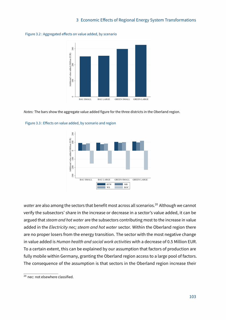
3 Economic E�ects of Regional Energy System Transformations
Figure 3.2 : Aggregated e�ects on value added, by scenario
010
020
030
0A
dditi
onal
val
ue a
dded
(Mill
ion
EUR
)
BAU SMALL BAU LARGE GREEN SMALL GREEN LARGE
Notes: The bars show the aggregate value added figure for the three districts in the Oberland region.
Figure 3.3 : E�ects on value added, by scenario and region
-300
-200
-100
010
020
0A
dditi
onal
val
ue a
dded
(Mill
ion
EUR
)
BAU SMALL BAU LARGE GREEN SMALL GREEN LARGE
BTW MBWS ROC
water are also among the sectors that benefit most across all scenarios.20 Althoughwe cannot
verify the subsectors’ share in the increase or decrease in a sector’s value added, it can be
argued that steam and hot water are the subsectors contributingmost to the increase in value
added in the Electricity nec; steam and hot water sector. Within the Oberland region there
are no proper losers from the energy transition. The sector with the most negative change
in value added is Human health and social work activitieswith a decrease of 0.5 Million EUR.
To a certain extent, this can be explained by our assumption that factors of production are
fully mobile within Germany, granting the Oberland region access to a large pool of factors.
The consequence of the assumption is that sectors in the Oberland region increase their
20 nec: not elsewhere classified.
103

3 Economic E�ects of Regional Energy System Transformations
production at the expenses of sectors in the rest of the country and not at the expenses of
other sectors within the region.
Figure 3.4 : E�ects on value added for selected sectors, GREEN LARGE scenario
-100 -50 0 50 100Additional value added (Million EUR)
ROC
INOLA
Wholesale and retail trade, repairs
Rubber, plastic, glass and ceramics
Rental & leasing; other business services
Real estate activities
Metals, machinery & equipment
Financial and insurance services
Electricity nec (incl. nuclear, oil); steam & hot water
Electricity from solar (PV and thermal)
Construction
Activities of membership organizations and other personal service activities
Notes: For a better visualization some sector descriptions have been shortened. See Appendix C.1 for the fullsector descriptions.
The careful reader might be missing conventional electricity sectors among the losers of
the energy transition. In fact, in the rest of the country value added in the sectors Electricity
from coal and Electricity from gas decreases, yet, only by about 5 Million Euro, corresponding
to a decrease of approximately 0.02% of these sectors’ value added in 2014. The almost
insignificant loss for these two sectors is more reassuring than worrying, given the small
size of the Oberland region compared to the rest of Germany. Since there are no coal power
plants in the Oberland region, there is no Electricity from coal sector in any of the districts and,
therefore, no value added losses.
3.4.2 E�ects on employment
The employment e�ects of the energy transition in the Oberland region are shown in Figure
3.5. Most of the increase occurs in medium-skilled employment, making up about 66% of the
104

3 Economic E�ects of Regional Energy System Transformations
Figure 3.5 : Aggregated e�ects on categories of employment in the Oberland region, by scenario
01,
000
2,00
03,
000
4,00
0A
dditi
onal
em
ploy
men
t (FT
E)
BAU SMALL BAU LARGE GREEN SMALL GREEN LARGE
Low-skilled Medium-skilledHigh-skilled
Figure 3.6 : E�ects on employment by category and region, GREEN LARGE scenario
-3,0
00-2
,000
-1,0
000
1,00
02,
000
Add
ition
al e
mpl
oym
ent (
FTE)
BTW MB WS ROC
Low-skilled Medium-skilledHigh-skilled
additional full time equivalent (FTE) jobs.21 Under the GREEN LARGE scenario, for instance,
the considered investments in renewables create 3,640 medium-skilled jobs in the region,
while the increase in high-skilled and low-skilled jobs is close to 1,460 and 400, respectively.22
In relative terms the increase in medium-skilled employments lies between 3% and 4.5%with
respect to the year 2014. For low-skilledandhigh-skilledemployment, thepercentage increase
is 2-2.9% vs. 1.6-2.4%, respectively. This implies that, in contrast to the absolute changes, the
relative increase in low-skilled employment is larger than in high-skilled employment.
21 Considering that in 2014medium-skilled labor accounted for 52% of employment across all categories, thisresult implies that the increase in medium-skilled labor is more than proportional to the pre-energy transitionshares.22 Note that, technically, we should rather refer to a reallocation of jobs instead of job creation, since we assumelabor to be scarce. However, interpreting the results as job creation in the region is not wrong per se, but weneed to keep in mind that this requires that jobs are “destroyed” somewhere else.
105

3 Economic E�ects of Regional Energy System Transformations
Figure 3.7 : Aggregated e�ects on employment by category, selected sectors and aggregated region, GREENLARGE scenario
-2,000 -1,000 0 1,000 2,000Additional employment (FTE)
ROC
INOLA
Wholesale and retail trade, repairsTransport, warehousing, post and telecom.
Rubber, plastic, glass and ceramicsRental & leasing; other business services
Metals, machinery & equipmentHuman health and social work activities
Hotels and restaurantsFinancial and insurance services
Construction
Wholesale and retail trade, repairsTransport, warehousing, post and telecom.
Rubber, plastic, glass and ceramicsRental & leasing; other business services
Metals, machinery & equipmentHuman health and social work activities
Hotels and restaurantsFinancial and insurance services
Construction
Low-skilled Medium-skilledHigh-skilled
Notes: For a better visualization some sector descriptions have been shortened. See Appendix C.1 for the fullsector descriptions.
Looking at the regional distribution of the employment e�ects, we see that it follows a pattern
similar to the e�ects on value added (see Figure 3.6 and Figures C.2 to C.4 in Appendix C.4).
The negative e�ects for the rest of the country in all three categories show that most of the
employment e�ects occurring in the Oberland region are job reallocations from the rest of
the country and, therefore, cannot be referred to as job creation. Note, however, that in light
of the findings of Buchheim et al. (2020), the employment results under the mobile labor
assumption can to some extent be understood as results for slack labor markets: when we
interpret labor from the rest of the country as coming from an unemployment pool. It has to
be noted though that in our model, these employees contributed to production in the rest of
the country before the “shock”, so it is not an accurate respresentation of unemployment.
Breaking down the employment e�ects in the GREEN LARGE scenario by sector delivers
the results in Figure 3.7.23 Considering the results presented so far, it is not surprising that
for medium-skilled labor the Construction sector exhibits the largest positive e�ects for the
23 A sector breakdown for the other scenarios can be found in Figures C.8-C.10.
106
3 Economic E�ects of Regional Energy System Transformations
Oberland region and the largest negative e�ects for the rest of the country. Electricity from
solar and Electricity nec; steamand hot water are among the sectors that benefit most in terms
of value added, yet, due to their low labor intensity, the employment e�ects in these sectors
are rather low.
3.5 Conclusions
In this investigation of the economic e�ects of an intended energy transition in the Bavarian
Oberland region we contribute to the literature in several ways. First, we disaggregate the
energy sector in the IO table to be able to consider the specificities of each technology’s
interlinkages with the rest of the economy. Second, we contribute to the literature on the
economic e�ects of regional investments, in a broader sense, andmore specifically, on the
e�ects of regional investments towards a transformation of the energy system. The key
contribution to this literature is the consideration of scarcities, which generate crowding out
e�ects both in the investment and in the operation phase. A third contribution consists in
expanding the approach developed by Fisher and Marshall (2011) Benz et al. (2014) to apply it
to an energy-related question and to improve its performance in a subnational context.
We show that following investments in a sector embedded in a framework where full employ-
ment and scarcity of financial resources is realistically assumed, value added and employment
in this and other sectors increase, but this comes at the expenses of other sectors and other
regions. We further show that assuming full mobility of factors of production within Germany,
gives the sectors in the Oberland region access to a very large pool of workers and capital,
that is, that of the rest of the country. Thus, the negative e�ects on other sectors are almost
fully “exported” to the region(s) where the investments do not take place. In our case the
decline in value added and employment occurs almost exclusively in sectors of the rest of the
country and not in our region of study. Moreover, we find that although employment in the
Oberland region increases in all three categories (low, medium and high-skilled), the increase
in medium-skilled employment is stronger than for the other two categories.
Thus, from the analysis of the employment e�ects of the intended energy transition in the
Bavarian Oberland region we can also draw conclusions for the whole of Germany and for
other countries with similar conditions. Irrespective of whether the energy transition occurs
at the regional or the national level, our results show that fundamentally restructuring the
107
3 Economic E�ects of Regional Energy System Transformations
energy system, as it is necessary to reduce greenhouse gas emissions in a serious manner,
requires an intensified employment of medium-skilled labor. Thus, considering that already
today Germany su�ers frommedium-skilled shortages, this can turn into a bottleneck for the
transformation of the energy system. We could expect market forces to fix the shortages by
increasing incentives (i.e., wages) in the demanded professions. Yet, the working of market
forces could take time, which is not available when talking about mitigating climate change.
The other, better option is to be proactive and increase the awareness for the importance of
these professions and their attractiveness as part of climate and energy policy interventions.
It is important to take into account that our analysis of the economic e�ects of a regional
energy transition is placed in a context where investments in renewable energies remain
constant outside of the Oberland region. If, on the contrary, other regions pursue a similar
goal or the energy transition at the national level is intensified, scarcities in the factors of
production would inhibit the achievement of the goals and therefore limit the positive e�ects
on the regional economy. Hence, further questions that arise in this context concern the
consequences of a far-reaching regionalization of the energy transition goal, that is, when
many regions intend to totally cover energy consumption by renewable energy generation.
In particular, an interesting question would be whether this regionalization could give rise
to a systems competition between the regions, seeking to attract capital (and labor) for the
respective energy transitions.
Possible extensions of the methodology could consider alternatives to our assumption of
full mobility of factors of production within Germany. On the one hand, the full mobility
assumption is a plausible assumption, specially for the production factor capital. On the other
hand, although in theory it is possible that workers move freely, there might also be frictions
binding workers to a specific region. A further development of our methodology could deal
with restricting mobility partially, so that it is possible to attract workers form other regions,
but to a limited extent. One possibility in this respect is to include neighboring districts in the
analysis to allowmobility within that larger region, but not with the rest of Germany. Finally,
modelling unemployment specific to sectors, regions and skill levels can be a useful addition
in light of the findings of Buchheim et al. (2020) and the current economic crisis.
108

Appendices
109

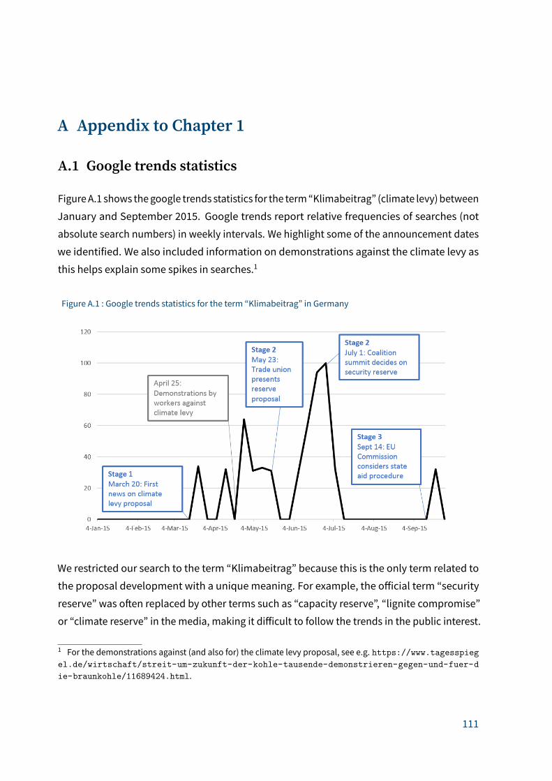
A Appendix to Chapter 1
A.1 Google trends statistics
FigureA.1 shows thegoogle trends statistics for the term“Klimabeitrag” (climate levy) between
January and September 2015. Google trends report relative frequencies of searches (not
absolute search numbers) in weekly intervals. We highlight some of the announcement dates
we identified. We also included information on demonstrations against the climate levy as
this helps explain some spikes in searches.1
Figure A.1 : Google trends statistics for the term “Klimabeitrag” in Germany
We restricted our search to the term “Klimabeitrag” because this is the only term related to
the proposal development with a uniquemeaning. For example, the o�icial term “security
reserve” was o�en replaced by other terms such as “capacity reserve”, “lignite compromise”
or “climate reserve” in the media, making it di�icult to follow the trends in the public interest.
1 For the demonstrations against (and also for) the climate levy proposal, see e.g. https://www.tagesspiegel.de/wirtschaft/streit-um-zukunft-der-kohle-tausende-demonstrieren-gegen-und-fuer-die-braunkohle/11689424.html.
111

A Appendix to Chapter 1
A.2 Details on the theoretical analysis
In this section, we provide further details about the theoretical analysis in Section 1.3.
A.2.1 Electricity market data
We obtain data on total load, renewable generation, and day ahead prices at the EEX for
German power market at hourly resolution from Open Energy Modeling Initiative (OEMI 2019).
We calculate the residual load as total load minus renewable electricity generation. Table A.1
presents a set of summary statistics for our main variables based on the raw 2015 electricity
market data for Germany. Figure A.2 illustrates the distribution of hourly electricity demand
and prices, where we only exclude negative prices. In our analysis, we truncate the prices at
the upper and lower 2nd percentiles which drops negative prices as well.
Table A.1 : Summary statistics for data on the electricity market
N Mean Median St. Dev. Min. Max.Total load (GW) 8760 59.46 59.03 10.56 36.15 79.89Renewable generation (GW) 8760 12.83 11.26 8.54 0.34 42.47Residual load (GW) 8760 46.63 46.48 11.75 9.39 78.50Price (Euro/MWh) 8759 31.63 30.54 12.66 -79.94 99.77
Notes: This table presents a set of summary statistics for our main variables basedon the raw 2015 electricity market data for Germany.
A.2.2 Capacity utilization
In order to conduct our scenario analysis, we have to rank alternative technologies based
on their marginal costs. Our ranking is based on the IEA’s cost projections. We depict the
implication of this strategy in Figure A.3, which shows the technological capacity ranges once
more, but together with the merit order curve and the residual load distribution. In order to
verify this strategy, we also illustrate the distribution of hourly average power generation by
technology in Figure A.4.2 Comparing these two figures verifies the imposedmerit order of
technologies as follows: The distribution for nuclear is le�-tailed, and the mass is close to its
full capacity. This evidence confirms that the nuclear capacity is rarely a marginal technology,
but o�en the infra-marginal technology. The picture for the gas capacity is just the opposite,
verifying that it is the marginal technology only at the high load instants.
2 We obtain these data from ENTSOE Transparency Data Platform.
112
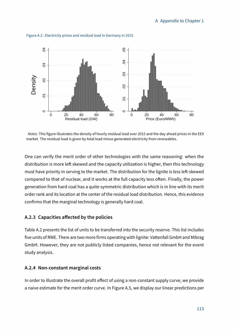
A Appendix to Chapter 1
Figure A.2 : Electricity prices and residual load in Germany in 2015
0.0
1.0
2.0
3.0
4
0 20 40 60 80Residual load (GW)
0.0
1.0
2.0
3.0
4.0
5
0 20 40 60 80Price (Euro/MWh)
De
nsity
Notes: This figure illustrates the density of hourly residual load over 2015 and the day ahead prices in the EEXmarket. The residual load is given by total loadminus generated electricity from renewables.
One can verify the merit order of other technologies with the same reasoning: when the
distribution is more le� skewed and the capacity utilization is higher, then this technology
must have priority in serving to the market. The distribution for the lignite is less le�-skewed
compared to that of nuclear, and it works at the full capacity less o�en. Finally, the power
generation from hard coal has a quite symmetric distribution which is in line with its merit
order rank and its location at the center of the residual load distribution. Hence, this evidence
confirms that the marginal technology is generally hard coal.
A.2.3 Capacities a�ected by the policies
Table A.2 presents the list of units to be transferred into the security reserve. This list includes
five units of RWE. There are twomore firms operatingwith lignite: Vattenfall GmbH andMibrag
GmbH. However, they are not publicly listed companies, hence not relevant for the event
study analysis.
A.2.4 Non-constant marginal costs
In order to illustrate the overall profit e�ect of using a non-constant supply curve, we provide
a naive estimate for the merit order curve. In Figure A.5, we display our linear predictions per
113

A Appendix to Chapter 1
Figure A.3 : Density of residual load and the merit order
Nuclear Lignite Hard coal Gas
020
40
60
0.0
1.0
2.0
3.0
4D
ensity
0 20 40 60 80Residual load (GW)
Merit order curve
Price
(E
uro
/MW
h)
Notes: This figure illustrates the density of daily residual load in 2015 by technology and the merit ordercurve used in our scenario analyses. The residual load is given by total loadminus generated electricity fromrenewables.
technology,whereweestimate the supply curve separately for eachcapacity rangedetermined
by the merit order of di�erent technologies. It is seen that the technology-specific fit is very
close to the fitted line to the full sample. In the rest of the section, we use these technology-
specific linear estimations.
Figure A.6 shows the e�ect of the climate levy on the supply curve, where the technological
capacities are illustrated for the baseline situation prior to the arrival of the policy shock.
We assume that the policies a�ect the lignite capacities with the highest marginal cost of
electricity production. The supply curve of the hard coal capacity shi�s to le�, and the a�ected
lignite capacity is relocated just to the le� of the gas capacity. Hence, the location of the gas
capacity does not change in this scenario. Note that this is not the case in the security reserve
scenario, where we simply remove the a�ected lignite capacity from the supply schedule.
We do not present the same figure for the security reserve scenario for brevity. However, we
illustrate the price and profit e�ects for both scenarios in the following analyses.
The predicted changes in prices are illustrated in Figure A.7 for both the climate levy and
the security reserve scenarios. This figure highlights several important points. First, there is
no shi� in the supply curve for the nuclear and una�ected lignite capacities. Therefore, the
114
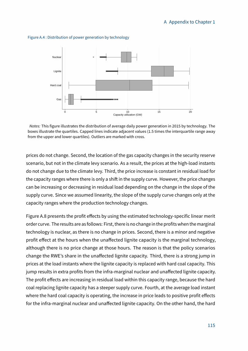
A Appendix to Chapter 1
Figure A.4 : Distribution of power generation by technology
0 5 10 15 20Capacity utilization (GW)
Gas
Hard coal
Lignite
Nuclear
Notes: This figure illustrates the distribution of average daily power generation in 2015 by technology. Theboxes illustrate the quartiles. Capped lines indicate adjacent values (1.5 times the interquartile range awayfrom the upper and lower quartiles). Outliers are marked with cross.
prices do not change. Second, the location of the gas capacity changes in the security reserve
scenario, but not in the climate levy scenario. As a result, the prices at the high-load instants
do not change due to the climate levy. Third, the price increase is constant in residual load for
the capacity ranges where there is only a shi� in the supply curve. However, the price changes
can be increasing or decreasing in residual load depending on the change in the slope of the
supply curve. Since we assumed linearity, the slope of the supply curve changes only at the
capacity ranges where the production technology changes.
Figure A.8 presents the profit e�ects by using the estimated technology-specific linear merit
order curve. The results are as follows: First, there is nochange in theprofitswhen themarginal
technology is nuclear, as there is no change in prices. Second, there is a minor and negative
profit e�ect at the hours when the una�ected lignite capacity is the marginal technology,
although there is no price change at those hours. The reason is that the policy scenarios
change the RWE’s share in the una�ected lignite capacity. Third, there is a strong jump in
prices at the load instants where the lignite capacity is replaced with hard coal capacity. This
jump results in extra profits from the infra-marginal nuclear and una�ected lignite capacity.
The profit e�ects are increasing in residual load within this capacity range, because the hard
coal replacing lignite capacity has a steeper supply curve. Fourth, at the average load instant
where the hard coal capacity is operating, the increase in price leads to positive profit e�ects
for the infra-marginal nuclear and una�ected lignite capacity. On the other hand, the hard
115

A Appendix to Chapter 1
Figure A.5 : Technology-specific linear fits
Nuclear Lignite Hard coal Gas
02
04
06
08
01
00
0 20 40 60 80
Day ahead prices AVC by technology (IEA, 2015)
Linear fit by technology Linear fit full sample
Price (
Euro
/MW
h)
Residual load (GW)
Notes: This figure illustrates the price and residual load observations, the linear fits per technology, the linearfit to the full sample, and the IEA’s cost projections. The prices are day-ahead prices in the EEX market in 2015.The residual load is given by total loadminus electricity generation from renewables.
Figure A.6 : Climate levy and the supply curve
Nuclear Lignite Hard coal GasNuclear Lignite Hard coal Gas
020
40
60
0.0
1.0
2.0
3.0
4D
ensity
0 20 40 60 80Residual load (GW)
Baseline Climate levy
Price
(E
uro
/MW
h)
Notes: This figure illustrates the changes in the supply curve for the climate levy scenario. The residual load isgiven by total loadminus generated electricity from renewables.
116

A Appendix to Chapter 1
Figure A.7 : Changes in prices
Nuclear Lignite Hard coal GasNuclear Lignite Hard coal Gas
02
46
0.0
1.0
2.0
3.0
4D
ensity
0 20 40 60 80Residual load (GW)
Baseline Security reserve
Price
(E
uro
/MW
h)
Notes: This figure illustrates the predicted changes in prices for the climate levy and the security reservescenarios. The residual load is given by total loadminus generated electricity from renewables.
Figure A.8 : Changes in profits
−150
−100
−50
050
0.0
1.0
2.0
3.0
4D
ensity
0 10 20 30 40 50 60 70 80Residual load (GW)
Climate levy Security reserve
Ch
an
ge
in
pro
fits
(E
uro
)
Notes: This figure illustrates the predicted changes in profits at each load instant for the climate levy and thesecurity reserve scenarios. The residual load is given by total loadminus generated electricity from renewables.
117

A Appendix to Chapter 1
Table A.2 : Phase-out schedule
Operator Name of unit Nameplatecapacity
Mothballing Decommissioning
Mibrag Buschhaus 352 MW Oct 1, 2016 Sep 30, 2020
RWE Frimmersdorf P 284 MW Oct 1, 2017 Sep 30, 2021Frimmersdorf Q 278 MW Oct 1, 2017 Sep 30, 2021Niederaußem E 295 MW Oct 1, 2018 Sep 30, 2022Niederaußem F 299 MW Oct 1, 2018 Sep 30, 2022Neurath C 292 MW Oct 1, 2019 Sep 30, 2023
Vattenfall Jänschwalde F 465 MW Oct 1, 2018 Sep 30, 2022Jänschwalde E 465 MW Oct 1, 2019 Sep 30, 2023
Source: StateAidDecisionText (SA.42536), ClosureofGermanLignitePlants: Letter to theMemberState. Availableat http://ec.europa.eu/competition/state_aid/cases/261321/261321_1762503_157_2.pdf.
coal capacity operating at the average load is now producing with higher marginal costs,
which exerts a negative pressure on the profits. The net e�ect is generally positive to the
le� of the average load and generally negative to the right. The reason is that, the share of
capacity operating with higher marginal cost is higher to the right of the average load instant.
Therefore, the profit e�ects become gradually negative at higher load instants.
We calculate the overall profit e�ects as the average of the profit changes weighted with the
residual load densities. Overall, we find that the climate levy causes 11%profit loss on average.
For the security reserve scenario, even without any compensation, our results indicate that
there is no change in profits on average (0.06% increase). This result shows that allowing
for non-constant marginal costs tends to reduce the negative profit e�ects compared to our
baseline assumption of constant marginal cost.
We conclude this section with some final remarks. The predicted price changes in this section
are quite high. Around the average load, the climate levy leads to amore than 5 Euros increase
in the equilibriumprice, and the security reserve scenario causes an increase around 2.5 Euros.
As a result the market equilibrium occurs at a higher price, which has a strong positive profit
e�ectoneachcapacityunit operatingatanaverage load instant, inparticular for infra-marginal
nuclear and una�ected lignite capacities. These predictions for price changes aremuch higher
than those in Oei et al. (2015), where the predicted price increase is minor. The explanation
might be that our naive estimate of the slope can be upward biased for several reasons. One
problem might be the linearity assumption. Note that the estimated technology-specific
lines form a quite smooth merit order curve. This result may be at odds with its common
118

A Appendix to Chapter 1
illustration with discrete jumps due to the presence of di�erent production technologies
in the supply schedule. In addition, one might expect its slope to be lower at lower load
instants and higher at higher load instants. However, we have verified our estimations by
conducting nonparametric robustness checks. A more likely problem is the simultaneity bias
in the estimations of reduced-form supply or demand functions. Identifying the supply curve
from data on equilibrium outcomes requires the demand to be fully inelastic. This might be
an extreme assumption at the hourly resolution, as consumers might have a certain degree of
flexibility in shi�ing their activity to di�erent hours in a day (Mier and Weissbart 2019).
A.3 Data and descriptive statistics
Our dataset is mainly from Thomson Reuters Datastream. The market return is based on
the DAX, a performance index consisting of the 30 major German companies trading on the
Frankfurt stock exchange. The continuously compounded returns are first di�erences of the
logarithmof prices. The descriptive statistics for the stock prices andmarket value of the three
utility firms, and the returns to DAX30 index are provided in Table A.3. Figure A.9 illustrates
the distribution of the returns for all three companies. The right panel excludes outliers to
ease comparison around the center of the distribution.
In Appendix A.5, we provide robustness tests by using oil prices and interest rates. Their
inclusion does not have any e�ect on the results. We use the crude oil spot price of Brent, FOB,
and the German three-month government bond benchmark rate as the risk-free rate of return.
The summary statistics for these additional variables are provided in Table A.3 along with our
main variables. The level of and the variation in the interest rates are very low throughout
2015. The returns to oil prices is characterized by many outliers. As a result these variables do
not addmuch to the explanatory power of the market model.
In using EnBW as a control unit, one concern might be that the results for EnBW are driven by
a company-specific characteristic that makes its assets immune to any type of shock. In this
case, using EnBW as a control unit would not eliminate the influence of a potential industry-
wide shock. In Figure A.9 it is clear that the distributions of returns are more or less the same
both at the tails and at the center. Therefore, it is not likely that the results for EnBW are driven
by a company-specific characteristic. Hence, using EnBW as a control unit seems a sensible
strategy.
119

A Appendix to Chapter 1
Table A.3 : Descriptive statistics
Units Mean Median St. Dev. Min. Max. Obs.Stock price - RWE € 18.392 19.789 5.330 9.219 25.684 261Stock price - E.ON € 10.253 10.853 1.957 6.331 12.889 261Stock price - EnBW € 24.120 24.800 1.660 19.866 26.759 261Market value - RWE bln. € 10.589 11.393 3.069 5.308 14.787 261Market value - E.ON bln. € 23.388 24.758 4.464 14.441 29.403 261Market value - EnBW bln. € 6.672 6.860 0.459 5.495 7.402 261Risk free rate % -0.001 -0.001 0.000 -0.002 -0.000 261Returns to DAX30 price index % 0.035 0.063 1.460 -4.816 4.852 261Returns to oil price % -0.188 0.000 2.346 -12.452 15.537 261
Notes: All values are based on 2015 data. Market value is equal to daily stock price times numberof outstanding shares.
Figure A.9 : Distribution of the returns
−.2
−.1
0.1
.2
EON EnBW RWE
−.0
50
.05
EON EnBW RWE
Re
turn
s
Notes: This figure illustrates the distribution of the returns for all three companies. The dots indicate outliers.The right panel excludes outliers.
120

A Appendix to Chapter 1
A.4 Details on estimation strategies
Our baseline estimation strategy is a short-run event study analysis. However, we use several
specifications and identification strategies. To layoutour assumptionsabout the identification
of anevent e�ect and to facilitate comparisonamongalternative estimators and specifications,
this section adopts a regression-based exposition of the short-run event study approach, while
we also explain how it is related to the classical exposition in the main text.3
Consider the following specification to assess the impact of a single event at date T on the
returns of a single asset i:
rit = Xitβi ++h∑d=−h
γdiDdt + εit, (A.1)
Almost all the elements of this specification has been introduced in the main text: rit is
the continuously compounded return of the asset at the trading date t,Xit is the vector of
covariates predicting the normal performance, and h is the half-width of the event window.
We ignore the pseudo window for brevity. The potential e�ect of the event on the returns is
captured by the set of event day dummies,Ddt = 1{τ = d}, where d = −h,−h+ 1, .., h and
the relative time index τ measures the distance to the event. Since the coe�icient vectors, βiand γdi , and the error term, εit, are asset specific, Equation (A.1) is asset specific.
In this specification, as the event day dummies capture the whole variation in the event
window, the eventwindowobservations are not relevant for the estimation of normal returns.4
As a result, this specification is equivalent to the approach described in the main text: the
event related abnormal return is given by γdi = ri,T+d − E[ri,T+d|Xi,T+d], and its estimate is
the prediction error, given by γdi = ri,T+d − ri,T+d. The null hypothesis that the event does
3 The short run event study methodology was introduced by Fama et al. (1969). See MacKinlay (1997) for adetailed description. The regression-based exposition is an alternative that is widely used in the literature. See,for example, Binder (1985a,b).4 Equation (A.1) excludes the event window observation in the estimation of expected returns as explainedearlier. The pseudo window can be introduced as follows:
rit = Xitβi +−h−1∑d=−ku
γdiDdt +
h∑d=−h
γdiDdt + εit, (A.2)
where the chosen relative distance to the announcement date is ku such that ku > h. The abnormal returnsbetween T − ku and T − h are expected to be insignificant, and can be used to conduct pseudo tests.
121
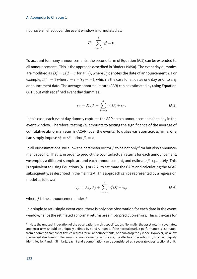
A Appendix to Chapter 1
not have an e�ect over the event window is formulated as:
H0:h∑
d=−h
γdi = 0.
To account for many announcements, the second term of Equation (A.1) can be extended to
all announcements. This is the approach described in Binder (1985a). The event day dummies
are modified asDdt = 1{d = τ for all j}, where Tj denotes the date of announcement j. For
example,D−1 = 1when τ = t− Tj = −1, which is the case for all dates one day prior to any
announcement date. The average abnormal return (AAR) can be estimated by using Equation
(A.1), but with redefined event day dummies.
rit = Xitβi +h∑
d=−h
γdiDdt + εit. (A.3)
In this case, each event day dummy captures the AAR across announcements for a day in the
event window. Therefore, testingH0 amounts to testing the significance of the average of
cumulative abnormal returns (ACAR) over the events. To utilize variation across firms, one
can simply impose γdi = γd and/or βi = β.
In all our estimations, we allow the parameter vector β to be not only firm but also announce-
ment specific. That is, in order to predict the counterfactual returns for each announcement,
we employ a di�erent sample around each announcement, and estimate β separately. This
is equivalent to using Equations (A.1) or (A.2) to estimate the CARs and calculating the ACAR
subsequently, as described in themain text. This approach can be represented by a regression
model as follows:
rijt = Xijtβij +h∑
d=−h
γdiDdt + εijt, (A.4)
where j is the announcement index.5
In a single asset - single event case, there is only one observation for each date in the event
window, hence theestimatedabnormal returns are simplypredictionerrors. This is the case for
5 Note the unusual indexation of the observations in this specification. Normally, the asset return, covariates,and error term should be uniquely defined by i and t. Indeed, if the normal market performance is estimatedfrom a common sample of firm i’s returns for all announcements, one can drop the j index. However, we allowthemarket structure to di�er around announcements. In this case, the e�ective time index is τ , which is uniquelyidentified by j and t. Similarly, each i and j combination can be considered as a separate cross-sectional unit.
122
A Appendix to Chapter 1
Equation (A.1) as it represents a separate regression for each firm and announcement. When
there are repeated observations for the event, in the form of many announcements or assets,
and if the specification includes commonevent day dummies across announcements or assets
as in Equations (A.3) and (A.4), then the estimation utilizes some of the variation in the event
window in the calculation of expected returns. In the following discussion, we use common
event day dummies for the sake of clarity and brevity. However, this is not our approach in
practice: we implement all our abnormal returns estimations as described in the main text by
excluding the event windows, and apply aggregation over assets or announcement expost.
The equivalent regression-based approach would be to define separate dummies for each
event day observation identified by (i, j, t). However, if the estimation windows are much
larger than the event windows, then both approaches lead to similar results. In our case, the
di�erences are ignorable.
A.4.1 Endogeneity of the market price index
Given the limited number of observations for the event e�ect, applying a synthetic control
approach (Abadie and Gardeazabal 2003) is an obvious, yet rarely pursued strategy in short-
run event studies. Its main requirement is to have su�icient observations in the pre-event
sample to form a control unit. Extrapolating the outcome variable of the control unit to the
event period and comparing it with the observed outcome of the a�ected units is the same
idea underlying both the short-run event study approach and the synthetic control approach.
Note that Equation (A.1) can be reformulated as a synthetic control estimation whereXitβi
can be considered the predicted outcome of the control unit. Then, the event e�ect is tested
on the di�erence between the observed outcome at the event date, riT , and the extrapolated
control outcome to the event date,XiT βi|T−h−1. Indeed, the usual control variable inXit, the
market index, is already a weighted average of asset prices in a given market. The problem is
that the event-a�ected units might participate in this portfolio, and the weights do not aim to
produce a proper counterfactual control unit for the a�ected company, rather to reflect the
average market conditions. The synthetic control approach allows to choose assets to form a
counterfactual portfolio and to estimate their weights.
Let i = 1 be the company that is hypothesized to be a�ected by the event. A synthetic
control is a weighted average of the units in the so-called donor pool of I units una�ected
by the event. Each choice of the vector of weightsW = (w2, ..., wI+1) such that 0≤wi≤1 and
123
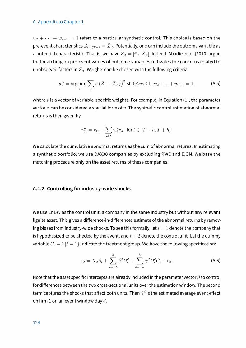
A Appendix to Chapter 1
w2 + · · · + wI+1 = 1 refers to a particular synthetic control. This choice is based on the
pre-event characteristicsZi,t<T−k = Zit. Potentially, one can include the outcome variable as
a potential characteristic. That is, we have Zit = [rit, Xit]. Indeed, Abadie et al. (2010) argue
that matching on pre-event values of outcome variables mitigates the concerns related to
unobserved factors in Zit. Weights can be chosen with the following criteria
w∗i = arg minwi
∑i
v(Z1 − Zi∈I
)2 st. 0≤wi≤1, w2 + ...+ wI+1 = 1, (A.5)
where v is a vector of variable-specific weights. For example, in Equation (1), the parameter
vector β can be considered a special form of v. The synthetic control estimation of abnormal
returns is then given by
γd1t = r1t −∑i∈I
w∗i rit, for t ∈ [T − h, T + h].
We calculate the cumulative abnormal returns as the sum of abnormal returns. In estimating
a synthetic portfolio, we use DAX30 companies by excluding RWE and E.ON. We base the
matching procedure only on the asset returns of these companies.
A.4.2 Controlling for industry-wide shocks
We use EnBW as the control unit, a company in the same industry but without any relevant
lignite asset. This gives a di�erence-in-di�erences estimate of the abnormal returns by remov-
ing biases from industry-wide shocks. To see this formally, let i = 1 denote the company that
is hypothesized to be a�ected by the event, and i = 2 denote the control unit. Let the dummy
variableCi = 1{i = 1} indicate the treatment group. We have the following specification:
rit = Xitβi +h∑
d=−h
δdDdt +
h∑d=−h
γdDdtCi + εit. (A.6)
Note that the asset specific intercepts are already included in the parameter vectorβ to control
for di�erences between the two cross-sectional units over the estimationwindow. The second
term captures the shocks that a�ect both units. Then γd is the estimated average event e�ect
on firm 1 on an event window day d.
124

A Appendix to Chapter 1
A.4.3 Other specifications
Intensity of the event. In some applications, there is a continuous variable measuring the
intensity of the potential event. For example, in one of our robustness analyses, we investigate
the e�ect of a confounding event: in this case, an earnings announcement. In this analysis, the
surprise in the earnings announcement is a continuous variable and if the announcement has
any e�ect, it is expected to be correlated with the magnitude of the surprise. Having repeated
observations for the event e�ect allows estimating the marginal abnormal returns due to the
surprise.
Denote the intensity of the surprise with sij . Then, Equation (A.4) can bemodified as follows:
rijt = Xijtβij +h∑
d=−h
γdiDdt sij + εijt. (A.7)
Here γdi is the marginal e�ect of the surprise. The abnormal return of firm i due to announce-
ment j is calculated as γdi sij .
Estimation window with repeated observations for the event e�ect. As explained ear-
lier, the specification inEquation (A.1) doesnot employany information fromtheeventwindow
to estimate the expected returns. This strategy can control for potential feedbacks from the
event to the normal market performance. However, this is not the case for Equations (A.4) and
(A.7), because the event dummies are assumed to be homogeneous across announcements
(or firms) and do not partial out the whole variation in the event window. Hence, one has to
include a dummy for each observational unit in the event window.
We take care of the feedback from the events to the normalmarket performance by estimating
the normal market performance separately from the pre-event observations. The return on a
day in the event window is predicted by ri,T+d = E[ri,T+d|Xi,T+d] = Xij,T+dβij|T−h−1, where
the estimated parameter vector is conditioned on the available information prior to the event
window. The abnormal return is then given by:
γdij = ri,T+d −Xij,T+dβij|T−h−1. (A.8)
As a result, the prediction of the expected returns does not employ any information from the
event window. In this case, the intensity of the event e�ect is estimated in a second-stage
125
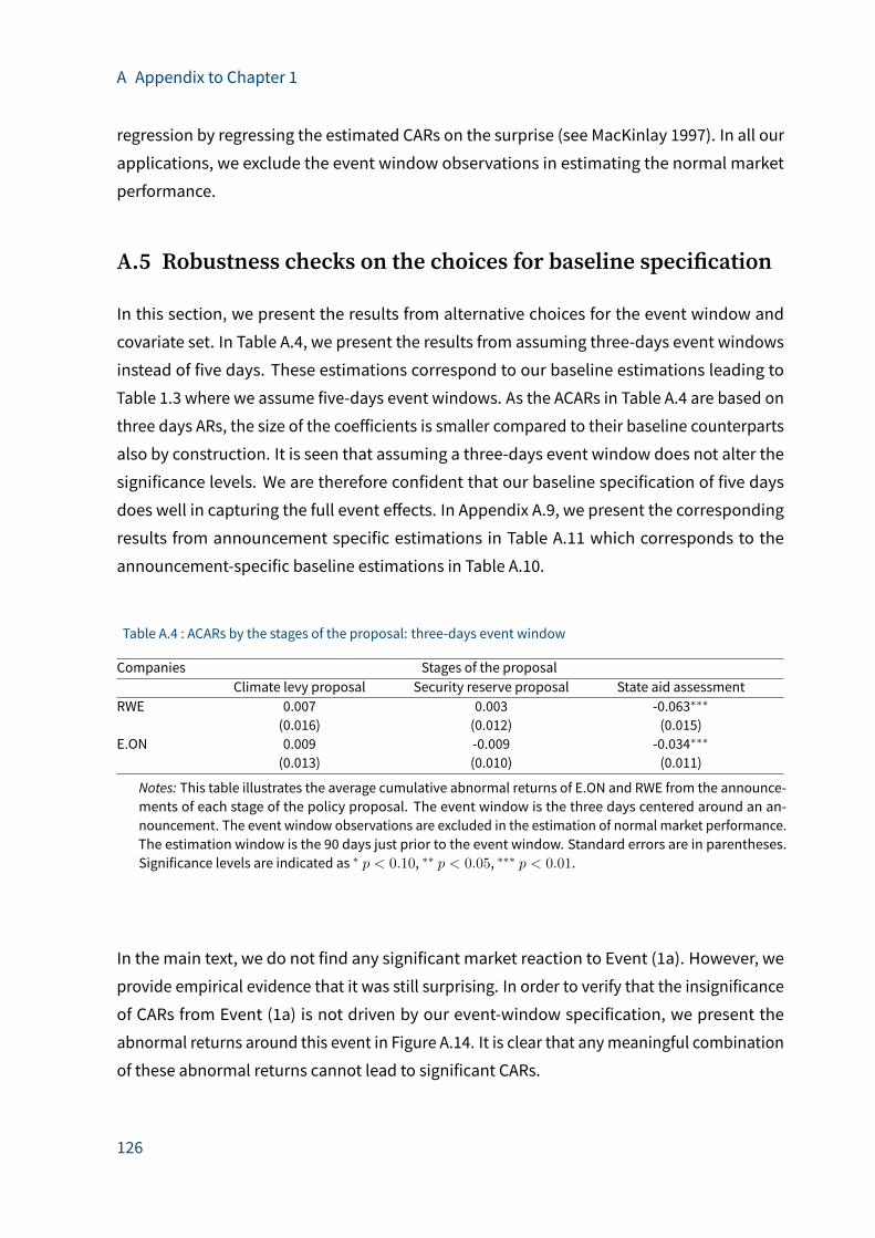
A Appendix to Chapter 1
regression by regressing the estimated CARs on the surprise (see MacKinlay 1997). In all our
applications, we exclude the event window observations in estimating the normal market
performance.
A.5 Robustness checks on the choices for baseline speci�cation
In this section, we present the results from alternative choices for the event window and
covariate set. In Table A.4, we present the results from assuming three-days event windows
instead of five days. These estimations correspond to our baseline estimations leading to
Table 1.3 where we assume five-days event windows. As the ACARs in Table A.4 are based on
three days ARs, the size of the coe�icients is smaller compared to their baseline counterparts
also by construction. It is seen that assuming a three-days event window does not alter the
significance levels. We are therefore confident that our baseline specification of five days
does well in capturing the full event e�ects. In Appendix A.9, we present the corresponding
results from announcement specific estimations in Table A.11 which corresponds to the
announcement-specific baseline estimations in Table A.10.
Table A.4 : ACARs by the stages of the proposal: three-days event window
Companies Stages of the proposalClimate levy proposal Security reserve proposal State aid assessment
RWE 0.007 0.003 -0.063∗∗∗
(0.016) (0.012) (0.015)E.ON 0.009 -0.009 -0.034∗∗∗
(0.013) (0.010) (0.011)
Notes: This table illustrates the average cumulative abnormal returns of E.ON and RWE from the announce-ments of each stage of the policy proposal. The event window is the three days centered around an an-nouncement. The event window observations are excluded in the estimation of normal market performance.The estimation window is the 90 days just prior to the event window. Standard errors are in parentheses.Significance levels are indicated as ∗ p < 0.10, ∗∗ p < 0.05, ∗∗∗ p < 0.01.
In the main text, we do not find any significant market reaction to Event (1a). However, we
provide empirical evidence that it was still surprising. In order to verify that the insignificance
of CARs from Event (1a) is not driven by our event-window specification, we present the
abnormal returns around this event in Figure A.14. It is clear that anymeaningful combination
of these abnormal returns cannot lead to significant CARs.
126
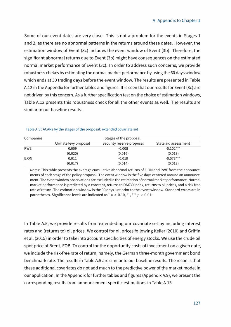
A Appendix to Chapter 1
Some of our event dates are very close. This is not a problem for the events in Stages 1
and 2, as there are no abnormal patterns in the returns around these dates. However, the
estimation window of Event (3c) includes the event window of Event (3b). Therefore, the
significant abnormal returns due to Event (3b) might have consequences on the estimated
normal market performance of Event (3c). In order to address such concerns, we provide
robustness chekcs by estimating the normalmarket performance by using the 60 dayswindow
which ends at 30 trading days before the event window. The results are presented in Table
A.12 in the Appendix for further tables and figures. It is seen that our results for Event (3c) are
not driven by this concern. As a further specification test on the choice of estimation windows,
Table A.12 presents this robustness check for all the other events as well. The results are
similar to our baseline results.
Table A.5 : ACARs by the stages of the proposal: extended covariate set
Companies Stages of the proposalClimate levy proposal Security reserve proposal State aid assessment
RWE 0.009 -0.008 -0.102∗∗∗
(0.020) (0.016) (0.019)E.ON 0.011 -0.019 -0.073∗∗∗
(0.017) (0.014) (0.013)
Notes: This table presents the average cumulative abnormal returns of E.ON and RWE from the announce-ments of each stage of the policy proposal. The event window is the five days centered around an announce-ment. The eventwindowobservations are excluded in the estimation of normalmarket performance. Normalmarket performance is predicted by a constant, returns to DAX30 index, returns to oil prices, and a risk freerate of return. The estimation window is the 90 days just prior to the event window. Standard errors are inparentheses. Significance levels are indicated as ∗ p < 0.10, ∗∗, ∗∗∗ p < 0.01.
In Table A.5, we provide results from extendeding our covariate set by including interest
rates and (returns to) oil prices. We control for oil prices following Keller (2010) and Gri�in
et al. (2015) in order to take into account specificities of energy stocks. We use the crude oil
spot price of Brent, FOB. To control for the opportunity costs of investment on a given date,
we include the risk-free rate of return, namely, the German three-month government bond
benchmark rate. The results in Table A.5 are similar to our baseline results. The reson is that
these additional covariates do not addmuch to the predictive power of the market model in
our application. In the Appendix for further tables and figures (Appendix A.9), we present the
corresponding results from announcement specific estimations in Table A.13.
127
A Appendix to Chapter 1
A.6 Robustness checks on the baseline distributionalassumption
In this section, we provide specification tests and robustness checks on the assumption of NID
disturbances. The first panel of Table A.6 presents the results from the estimation of normal
market performance. For brevity, we focus on the announcements in stage 3. The second
panel presents the p-values from various specification tests on the residuals. The Durbin test
is for serial correlation where the null hypothesis is there is no serial correlation up to fi�h
order. The null is rejected if any lags of the residuals is significant in an auxiliary regression of
the residuals on its lags. The null for the LM (Engle’s Lagrangemultiplier) tests is that there
is no pth order autoregressive conditional heteroscedasticity (ARCH(p)) in the residuals. The
third panel presents the alternative estimates for the standard errors: (i) robust standard
errors for arbitrary forms of heteroscedasticity, (ii) standard errors based on pair-bootstraping,
and (iii) Newey-West standard errors taking into account up to fi�h order autocorrelations.
According to the results from the Durbin tests and the LM tests for ARCH(p) e�ects, there is no
sign for serial correlation or heteroscedaticity. This result is further confirmed by the results
in the third panel. The alternative estimates of standard errors are very close to our baseline
estimates. There is only one exception to this general result, where the Durbin test rejects the
null in the fi�h column. However, the baseline and the Newey-West standard errors are still
very close to each other, suggesting that the influence of significant lag order is minor.
Figure A.10 illustrates the prediction intervals based on bootstrapping. Here, the contribu-
tion of sampling uncertainty is calculated based on pair-bootstrapped standard errors. As
mentioned in the main text, this type of uncertainty is typically small which is the case in our
application too. Therefore, the estimationmethod for sampling uncertainty have almost no
influence on the width of the prediction intervals. In Figure A.10, we assume IID errors in esti-
mating the error uncertainty by resampling OLS-residuals with replacement (1000 repetitions)
which is robust to departures from normality assumption. The width of these confidence
intervals are close to their baseline counterparts. Table A.7 presents the bootstrapped stan-
dard errors calculated from the empirical distribution of resampled OLS residuals. Again, the
results are very close to their baseline counterparts.
128

A Appendix to Chapter 1
Table A.6 : Specification tests and alternative estimates of standard errors
RWE-(3a) RWE-(3b) RWE-(3c) E.ON-(3a) E.ON-(3b) E.ON-(3c)DAX30 Market Return 0.669 0.699 0.864 0.710 0.701 0.784
(0.104) (0.090) (0.106) (0.080) (0.070) (0.066)Durbin test 0.683 0.255 0.521 0.506 0.063 0.355LM test - order 1 0.997 0.626 0.716 0.391 0.717 0.421LM test - order 3 0.875 0.824 0.908 0.484 0.796 0.797LM test - order 5 0.929 0.911 0.976 0.320 0.797 0.903Robust s.e. 0.087 0.076 0.106 0.075 0.065 0.090Bootstrap s.e. 0.090 0.080 0.108 0.078 0.067 0.090Newey-West s.e. 0.091 0.083 0.099 0.075 0.064 0.074
Notes: The first panel presents the results from the OLS estimation of normal market performance. Thesecond panel presents the p-values from various specification tests on the residuals. The Durbin test is forserial correlation where the null hypothesis is there is no serial correlation up to pth order. The null for theLM (Engle’s Lagrangemultiplier) tests is there is no pth order autoregressive conditional heteroscedasticity(ARCH(p)) in the residuals. The third panel presents the alternative estimates for the standard errors. Boot-strap standard errors are based on 1000 replications. The estimation of Newey-West standard errors includeall the lags of the residuals up to fi�h order.
Table A.7 : CARs and bootstrapped standard errors
Companies Announcements(3a) (3b) (3c)
RWE
E.ON
-0.020 (0.033) 0.004
( 0.025)
-0.135∗∗∗
(0.032)-0.000 (0.024)
-0.150∗∗∗
(0.036)-0.220∗∗∗
(0.028)
Notes: This table presents the cumulative abnormal returns of RWE and E.ON from each announcement in the third stage of the policy proposal. The event window is the five days centered around an announcement. The estimation window is the 90 days just prior to the event window. Hence, the event window observations
are excluded in the estimation of normal market performance. Bootstrapped standard errors are in parentheses. Significance levels are indicated as ∗ p < 0.10, ∗∗ p < 0.05, ∗∗∗ p < 0.01.
129
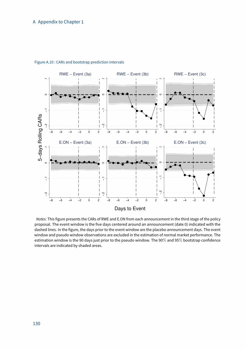
A Appendix to Chapter 1
Figure A.10 : CARs and bootstrap prediction intervals
−.2
−.1
0.1
−8 −6 −4 −2 0 2
RWE − Event (3a)
−.2
−.1
0.1
−8 −6 −4 −2 0 2
RWE − Event (3b)
−.2
−.1
0.1
−8 −6 −4 −2 0 2
RWE − Event (3c)
−.2
−.1
0.1
−8 −6 −4 −2 0 2
E.ON − Event (3a)
−.2
−.1
0.1
−8 −6 −4 −2 0 2
E.ON − Event (3b)
−.2
−.1
0.1
−8 −6 −4 −2 0 2
E.ON − Event (3c)
5−
days R
olli
ng C
AR
s
Days to Event
Notes: This figure presents the CARs of RWE and E.ON from each announcement in the third stage of the policyproposal. The event window is the five days centered around an announcement (date 0) indicated with thedashed lines. In the figure, the days prior to the event window are the placebo announcement days. The eventwindow and pseudo window observations are excluded in the estimation of normal market performance. Theestimation window is the 90 days just prior to the pseudo window. The 90% and 95% bootstrap confidenceintervals are indicated by shaded areas.
130

A Appendix to Chapter 1
A.7 Confounding events investigation
This section presents details on the search for potential confounding events around announce-
ments (3b) and (3c). We conducted a search for English- and German-language news in Lexis-
Nexis for the five-day window (working days) around each of these announcements, filtering
by company name (RWE or E.ON, respectively). We restricted the search to business news in
newswires and press releases to avoid a large number of news items appearingmultiple times.
Still, we were faced with a large number of very diverse news items in the event window for
each firm.
We thereforemanually categorized the news items according to their content and counted the
number of news items on a specific topic in the given event window. We then assessed, based
on content and press coverage, whether the news topics could be relevant drivers for the
stock performance we observe in our event window. When we identified a potential company-
specific confounding event for announcement (2b), we performed robustness analyses (see
Section 1.7.2 for robustness checks on earnings announcements). For announcement (3c),
we are more concerned with news that a�ects both RWE and E.ON, and thus performed
robustness analyses for the case of a potential industry confounding event. Here we identified
thenuclearprovisioning issueasoutlined inSection1.7.2. LexisNexis providesagoodoverview
of important issues around the event dates, but it was essential to complement this with own
research on the events identified as potentially confounding. For instance, we found that the
German business newspaper Handelsblatt was the first to report on the nuclear provisioning
report on September 11; however, the first news items in LexisNexis mentioning this in the
context of RWE appear on September 15.
In Appendix A.9, Tables A.17, A.18, A.19, and A.20 present the main news topics and numbers
of news items on these topics for each company and each event window.
A.8 Estimation of earnings surprise
E�ects of earnings announcements. We start by investigating the information content of
quarterly earnings announcements for the market valuation of RWE and E.ON. If there is any
investor reaction to earnings announcements, it should be due to the departure of announced
earnings from investors’ prior expectations, namely, the surprise in the information release.
131
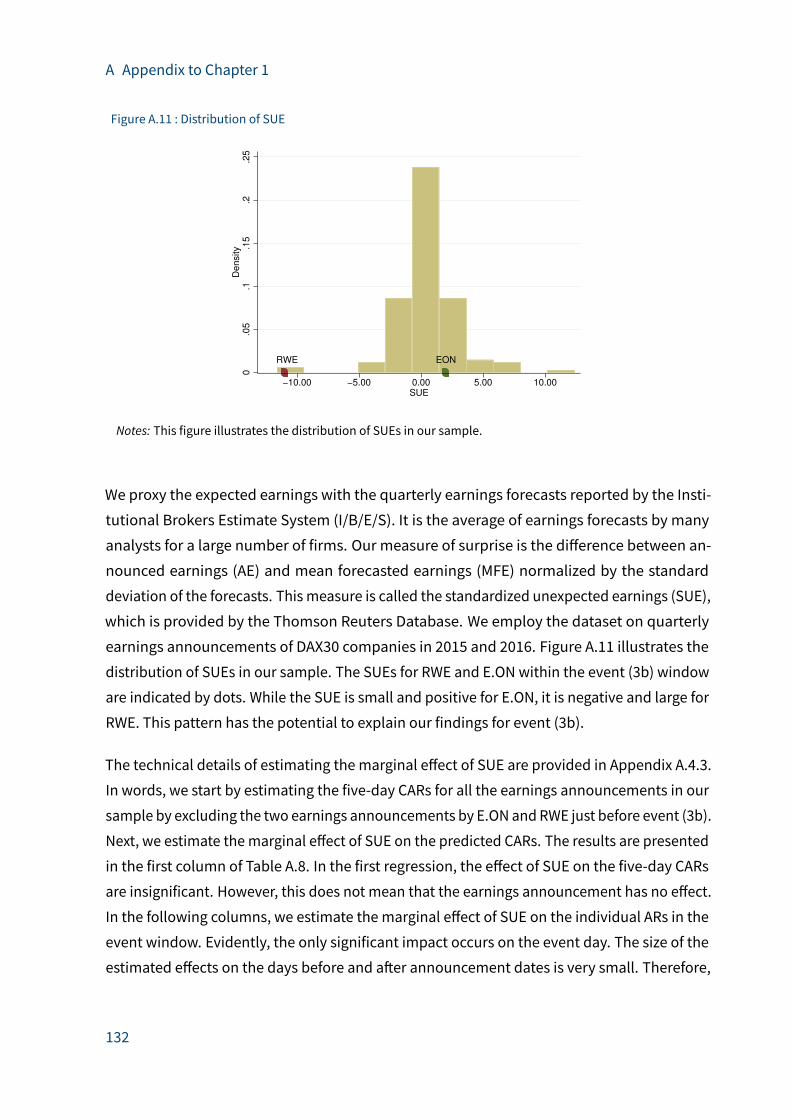
A Appendix to Chapter 1
Figure A.11 : Distribution of SUE
RWE EON
0.0
5.1
.15
.2.2
5D
ensity
−10.00 −5.00 0.00 5.00 10.00SUE
Notes: This figure illustrates the distribution of SUEs in our sample.
We proxy the expected earnings with the quarterly earnings forecasts reported by the Insti-
tutional Brokers Estimate System (I/B/E/S). It is the average of earnings forecasts by many
analysts for a large number of firms. Our measure of surprise is the di�erence between an-
nounced earnings (AE) and mean forecasted earnings (MFE) normalized by the standard
deviation of the forecasts. This measure is called the standardized unexpected earnings (SUE),
which is provided by the Thomson Reuters Database. We employ the dataset on quarterly
earnings announcements of DAX30 companies in 2015 and 2016. Figure A.11 illustrates the
distribution of SUEs in our sample. The SUEs for RWE and E.ON within the event (3b) window
are indicated by dots. While the SUE is small and positive for E.ON, it is negative and large for
RWE. This pattern has the potential to explain our findings for event (3b).
The technical details of estimating the marginal e�ect of SUE are provided in Appendix A.4.3.
In words, we start by estimating the five-day CARs for all the earnings announcements in our
sample by excluding the two earnings announcements by E.ON and RWE just before event (3b).
Next, we estimate themarginal e�ect of SUE on the predicted CARs. The results are presented
in the first column of Table A.8. In the first regression, the e�ect of SUE on the five-day CARs
are insignificant. However, this does not mean that the earnings announcement has no e�ect.
In the following columns, we estimate the marginal e�ect of SUE on the individual ARs in the
event window. Evidently, the only significant impact occurs on the event day. The size of the
estimated e�ects on the days before and a�er announcement dates is very small. Therefore,
132
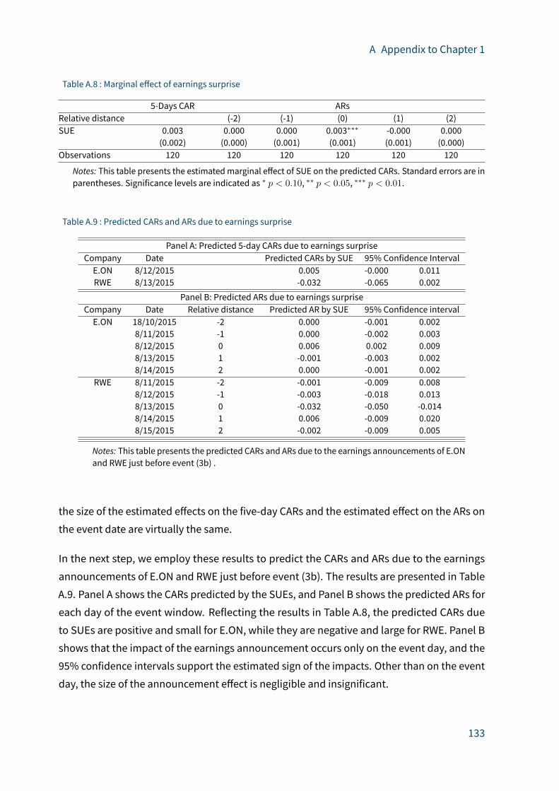
A Appendix to Chapter 1
Table A.8 : Marginal e�ect of earnings surprise
5-Days CAR ARsRelative distance (-2) (-1) (0) (1) (2)SUE 0.003 0.000 0.000 0.003∗∗∗ -0.000 0.000
(0.002) (0.000) (0.001) (0.001) (0.001) (0.000)Observations 120 120 120 120 120 120
Notes: This table presents the estimatedmarginal e�ect of SUE on the predicted CARs. Standard errors are inparentheses. Significance levels are indicated as ∗ p < 0.10, ∗∗ p < 0.05, ∗∗∗ p < 0.01.
Table A.9 : Predicted CARs and ARs due to earnings surprise
Panel A: Predicted 5-day CARs due to earnings surpriseCompany Date Predicted CARs by SUE 95% Confidence IntervalE.ON 8/12/2015 0.005 -0.000 0.011RWE 8/13/2015 -0.032 -0.065 0.002
Panel B: Predicted ARs due to earnings surpriseCompany Date Relative distance Predicted AR by SUE 95% Confidence intervalE.ON 18/10/2015 -2 0.000 -0.001 0.002
8/11/2015 -1 0.000 -0.002 0.0038/12/2015 0 0.006 0.002 0.0098/13/2015 1 -0.001 -0.003 0.0028/14/2015 2 0.000 -0.001 0.002
RWE 8/11/2015 -2 -0.001 -0.009 0.0088/12/2015 -1 -0.003 -0.018 0.0138/13/2015 0 -0.032 -0.050 -0.0148/14/2015 1 0.006 -0.009 0.0208/15/2015 2 -0.002 -0.009 0.005
Notes: This table presents the predicted CARs and ARs due to the earnings announcements of E.ONand RWE just before event (3b) .
the size of the estimated e�ects on the five-day CARs and the estimated e�ect on the ARs on
the event date are virtually the same.
In the next step, we employ these results to predict the CARs and ARs due to the earnings
announcements of E.ON and RWE just before event (3b). The results are presented in Table
A.9. Panel A shows the CARs predicted by the SUEs, and Panel B shows the predicted ARs for
each day of the event window. Reflecting the results in Table A.8, the predicted CARs due
to SUEs are positive and small for E.ON, while they are negative and large for RWE. Panel B
shows that the impact of the earnings announcement occurs only on the event day, and the
95% confidence intervals support the estimated sign of the impacts. Other than on the event
day, the size of the announcement e�ect is negligible and insignificant.
133

A Appendix to Chapter 1
Figure A.12 : E�ect of announcement (3b) corrected for earnings surprise
−.2
−.1
0.1
−8 −7 −6 −5 −4 −3 −2 −1 0 1 2
CAR: Event (3b) − RWE
−.2
−.1
0.1
−8 −7 −6 −5 −4 −3 −2 −1 0 1 2
CAR: Event (3b) − E.ON
−.1
−.0
50
.05
−10 −9 −8 −7 −6 −5 −4 −3 −2 −1 0 1 2
AR: Event (3b) − RWE
−.1
−.0
50
.05
−10 −9 −8 −7 −6 −5 −4 −3 −2 −1 0 1 2
AR: Event (3b) − E.ON
Days to Event
Notes: This figure presents the ARs and CARs of E.ON and RWE from announcement (3b) corrected for theearnings announcements. The event window is the five days centered around an announcement (date 0)indicated with the dashed lines. The days prior to the event window are the placebo announcement days. Theevent window and pseudo window observations are excluded in the estimation of normal market performance.The estimation window is the 90 days just prior to the pseudo window. The 90% and 95% confidence intervalsfor the (uncorrected CARs) are presented as forecast intervals (shaded areas). The 90% confidence interval ofpredicted e�ect of earnings announcement is illustrated around the corrected CARs.
Correcting for the e�ect of earnings announcements. The rolling CARs and the ARs, cor-
rected for the size of the predicted earnings announcement e�ect, are presented in Figure
A.12. This figure di�ers from the one presented in the main text in two ways. First, this fig-
ure illustrates the two sources of uncertainity, rather than the aggregated one presented
in themain text. Second, the correction assumes a five-day event window for the earnings
announcement. For example, the correction for RWE includes the dates between -3 and 1,
as the earnings announcement of RWE is on date -1. This is also a conservative approach
given that our results reveal that the e�ect of the earnings announcements is taking place
134
A Appendix to Chapter 1
on the announcement date only. The figure also illustrates the 90% confidence interval of
the predicted earnings announcement e�ect constructed around the corrected CARs and
ARs. The e�ect of the correction on CARs extends beyond the correction window due to the
aggregation of ARs across days.
Figure A.12 confirms the results presented in the main text and illustrates its details. An
informal and conservative inference strategy is to compare the 90% confidence intervals. It
is conservative, because a formal comparison requires calculating the standard error of the
di�erence of these two random e�ects as in the main text. In our case, assuming that these
twoperedictions are uncorrelated is reasonable due to theway that these e�ects are predicted
by using di�erent samples. In this case, the standard error of the di�erence is equal to the
square-root of the sumof variances. The standard error of the net e�ect is always smaller than
the sum of the standard errors of the two predictions. Hence, the formal confidence interval,
presented in the main text, is smaller than the sum of the confidence intervals of these two
e�ects. However, Figure A.12 is useful to illustrate the confidence intervals separately for
expositional clarity. It is seen that the confidence intervals of the corrected CAR on the event
day (day 0) and the predicted returns do not overlap. Figure A.12 do not present the 95%
confidence interval for the corrected CAR, which do overlap slightly. As a result, the corrected
e�ect of event (3b) is still significant at reasonable levels, but much smaller than the baseline
estimate.
135

A Appendix to Chapter 1
A.9 Additional tables and �gures
Table A.10 : CARs by announcement: baseline specification
Stages Announcements CompaniesRWE E.ON EnBW
Climate levy proposal 1a 0.033 0.040 -0.004(0.034) (0.029) (0.039)
1b 0.004 -0.011 -0.014(0.035) (0.029) (0.039)
1c -0.002 0.005 0.007(0.035) (0.028) (0.042)
Security reserve 2a -0.004 -0.029 0.014(0.033) (0.027) (0.044)
2b -0.033 -0.028 0.017(0.032) (0.027) (0.043)
2c -0.002 -0.013 -0.007(0.030) (0.028) (0.048)
2d 0.012 -0.007 0.011(0.030) (0.027) (0.049)
State aid assessment 3a -0.020 0.004 -0.001(0.031) (0.024) (0.050)
3b -0.135∗∗∗ 0.000 -0.004(0.028) (0.021) (0.050)
3c -0.150∗∗∗ -0.220∗∗∗ -0.017(0.038) (0.024) (0.050)
Notes: This table presents the cumulative abnormal returns of all companies due to each announcement.The event window is the five days centered around an announcement. The estimation window is the 90days just prior to the event window. Hence, the event window observations are excluded in the estimationof normal market performance. Standard errors are in parentheses. Significance levels are indicated as ∗
p < 0.10, ∗∗ p < 0.05, ∗∗∗ p < 0.01.
136

A Appendix to Chapter 1
Table A.11 : CARs by announcement: three-day event window
Stages Announcements CompaniesRWE E.ON EnBW
Climate levy proposal 1a 0.000 0.012 0.020(0.027) (0.023) (0.031)
1b 0.025 0.006 0.005(0.027) (0.023) (0.030)
1c -0.003 0.010 0.014(0.027) (0.021) (0.032)
Security reserve proposal 2a -0.006 -0.026 0.024(0.026) (0.021) (0.033)
2b -0.013 0.003 -0.002(0.025) (0.021) (0.034)
2c 0.003 -0.019 -0.026(0.023) (0.021) (0.037)
2d 0.027 0.006 -0.002(0.022) (0.020) (0.038)
State aid assessment 3a -0.004 0.000 0.015(0.024) (0.018) (0.039)
3b -0.108∗∗∗ -0.010 -0.006(0.021) (0.017) (0.039)
3c -0.076∗∗∗ -0.092∗∗∗ -0.016(0.029) (0.021) (0.038)
Notes: This table presents the cumulative abnormal returns of all companies due to each announcement.The event window is the three days centered around an announcement. The event window observations areexcluded in the estimation of normal market performance. The estimation window is the 90 days just priorto the event window. Standard errors are in parentheses. Significance levels are indicated as ∗ p < 0.10, ∗∗
p < 0.05, ∗∗∗ p < 0.01.
137

A Appendix to Chapter 1
Table A.12 : CARs by announcement: robustness to estimation window
Stages Announcements CompaniesRWE E.ON EnBW
Climate levy proposal 1a 0.036 0.041 -0.002(0.035) (0.028) (0.040)
1b 0.010 -0.008 -0.014(0.034) (0.028) (0.042)
1c 0.000 0.009 0.005(0.038) (0.029) (0.034)
Security reserve proposal 2a -0.009 -0.026 0.015(0.036) (0.029) (0.034)
2b -0.038 -0.025 0.018(0.034) (0.030) (0.040)
2c -0.003 -0.013 0.002(0.033) (0.030) (0.046)
2d 0.009 -0.016 0.004(0.033) (0.028) (0.044)
State aid assessments 3a -0.018 -0.002 -0.013(0.030) (0.025) (0.048)
3b -0.133∗∗∗ 0.001 -0.004(0.026) (0.023) (0.057)
3c -0.162∗∗∗ -0.225∗∗∗ -0.014(0.029) (0.022) (0.047)
Notes: This table presents the cumulative abnormal returns of all companies due to each announcement.The event window is the five days centered around an announcement. The event window observations areexcluded in the estimation of normal market performance. The estimation window is the 60 days windowending at 30 days prior to the event window. Standard errors are in parentheses. Significance levels areindicated as ∗ p < 0.10, ∗∗ p < 0.05, ∗∗∗ p < 0.01.
138
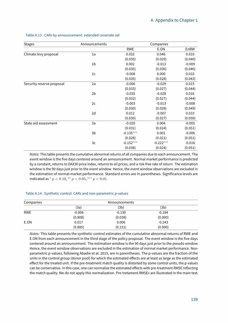
A Appendix to Chapter 1
Table A.13 : CARs by announcement: extended covariate set
Stages Announcements CompaniesRWE E.ON EnBW
Climate levy proposal 1a 0.032 0.046 0.010(0.035) (0.029) (0.040)
1b 0.002 -0.013 -0.009(0.035) (0.030) (0.040)
1c -0.008 0.000 0.010(0.035) (0.028) (0.043)
Security reserve proposal 2a -0.006 -0.029 0.015(0.033) (0.027) (0.044)
2b -0.035 -0.028 0.016(0.032) (0.027) (0.044)
2c -0.003 -0.013 -0.008(0.030) (0.028) (0.049)
2d 0.012 -0.007 0.010(0.030) (0.027) (0.050)
State aid assessment 3a -0.020 0.004 -0.005(0.031) (0.024) (0.051)
3b -0.135∗∗∗ 0.001 -0.006(0.028) (0.021) (0.051)
3c -0.152∗∗∗ -0.222∗∗∗ -0.016(0.038) (0.024) (0.051)
Notes: This table presents the cumulative abnormal returns of all companies due to each announcement. Theevent window is the five days centered around an announcement. Normal market performance is predictedby a constant, returns to DAX30 price index, returns to oil prices, and a risk-free rate of return. The estimationwindow is the 90 days just prior to the event window. Hence, the event window observations are excluded inthe estimation of normal market performance. Standard errors are in parentheses. Significance levels areindicated as ∗ p < 0.10, ∗∗ p < 0.05, ∗∗∗ p < 0.01.
Table A.14 : Synthetic control: CARs and non-parametric p-values
Companies Announcements(3a) (3b) (3b)
RWE -0.006 -0.130 -0.184(0.808) (0.038) (0.000)
E.ON 0.017 0.006 -0.243(0.885) (0.231) (0.000)
Notes: This table presents the synthetic-control estimates of the cumulative abnormal returns of RWE andE.ON from each announcement in the third stage of the policy proposal. The event window is the five dayscentered around an announcement. The estimation window is the 90 days just prior to the pseudo window.Hence, the event window observations are excluded in the estimation of normal market performance. Non-parametric p-values, following Abadie et al. 2015, are in parentheses. The p-values are the fraction of theunits in the control group (donor pool) for which the estimated e�ects are at least as large as the estimatede�ect for the treated unit. If the pre-treatment match quality is distorted by some control units, the p-valuescan be conservative. In this case, one can normalize the estimated e�ects with pre-treatment RMSE reflectingthe match quality. We do not apply this normalization. Pre-tretament RMSEs are illustrated in the main text.
139
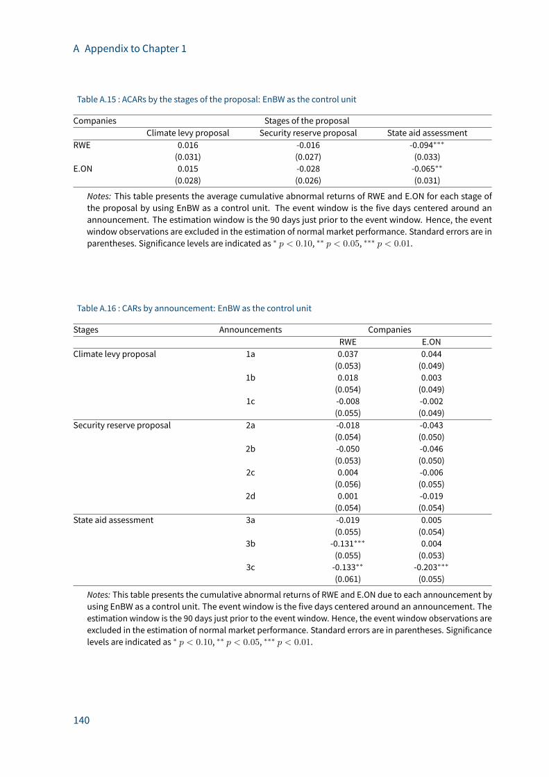
A Appendix to Chapter 1
Table A.15 : ACARs by the stages of the proposal: EnBW as the control unit
Companies Stages of the proposalClimate levy proposal Security reserve proposal State aid assessment
RWE 0.016 -0.016 -0.094∗∗∗
(0.031) (0.027) (0.033)E.ON 0.015 -0.028 -0.065∗∗
(0.028) (0.026) (0.031)
Notes: This table presents the average cumulative abnormal returns of RWE and E.ON for each stage ofthe proposal by using EnBW as a control unit. The event window is the five days centered around anannouncement. The estimation window is the 90 days just prior to the event window. Hence, the eventwindow observations are excluded in the estimation of normal market performance. Standard errors are inparentheses. Significance levels are indicated as ∗ p < 0.10, ∗∗ p < 0.05, ∗∗∗ p < 0.01.
Table A.16 : CARs by announcement: EnBW as the control unit
Stages Announcements CompaniesRWE E.ON
Climate levy proposal 1a 0.037 0.044(0.053) (0.049)
1b 0.018 0.003(0.054) (0.049)
1c -0.008 -0.002(0.055) (0.049)
Security reserve proposal 2a -0.018 -0.043(0.054) (0.050)
2b -0.050 -0.046(0.053) (0.050)
2c 0.004 -0.006(0.056) (0.055)
2d 0.001 -0.019(0.054) (0.054)
State aid assessment 3a -0.019 0.005(0.055) (0.054)
3b -0.131∗∗∗ 0.004(0.055) (0.053)
3c -0.133∗∗ -0.203∗∗∗
(0.061) (0.055)
Notes: This table presents the cumulative abnormal returns of RWE and E.ON due to each announcement byusing EnBW as a control unit. The event window is the five days centered around an announcement. Theestimation window is the 90 days just prior to the event window. Hence, the event window observations areexcluded in the estimation of normal market performance. Standard errors are in parentheses. Significancelevels are indicated as ∗ p < 0.10, ∗∗ p < 0.05, ∗∗∗ p < 0.01.
140

A Appendix to Chapter 1
Table A.17 : Type and number of company-related news around event (3b), RWE
Topic Wed 12/08 Thu 13/08 Fri 14/08 Mon 17/08 Tue 18/08
Earnings announcements (EA), financials 1 9 1Background on EA, company strategy 2 6Voting rights announcements 4Investments of company 2 5 3Personnel appointments 2Other 2
Source: Own summary based on LexisNexis, German- and English-language newswires andpress releases, filteredby date and company name. “Other” includes local activities such as Czech gas management and local protests.
Table A.18 : Type and number of company-related news around event (3b), E.ON
Topic Wed 12/08 Thu 13/08 Fri 14/08 Mon 17/08 Tue 18/08
Earnings announcements (EA), financials 7EA and background, company strategy 16 6E.ON Russia financials 7 15 1E.ON UK financials 1 1 2 1 1Voting rights announcements 5Investments of company 5 2Other 2 4 2
Source: Own summary based on LexisNexis, German- and English-language newswires andpress releases, filteredby date and company name. “Other” includes local activities such as the opening of a plant, school visits, publicrelation activities related to a wind farm, etc., or the mentioning of E.ON in news about other firms. News itemsfrom Saturday and Sunday are assigned to the following Monday.
141

A Appendix to Chapter 1
Table A.19 : Type and number of company-related news around event (3c), RWE
Topic Thu 10/09 Fri 11/09 Mon 14/09 Tue 15/09 Wed 16/09
Tendering and contracting 6 4Issues with power plant permissions 4 1 1 2Personnel issues 1 4Background on past stock performance 4 1Pending lawsuits 6 4Local operations & PR 6 1General industry news (gas supply) 4 2Nuclear provisioning Germany 1 7Other 1 1 3 2
Notes: Industry-wide news in bold.Source: Own summary based on LexisNexis, German- and English-language newswires andpress releases, filteredby date and company name. News items from Saturday are assigned to the following Monday. “Pending lawsuits”relates to a gas procurement conflict where RWE may need to pay a penalty, for part of which the companyalready booked provisions. “Issues with power plant permissions” involve wind farm projects (new proposala�er rejection) and a coal-fired power plant (court ruling that permit is upheld). “General industry news on gassupply” is a report on Iran as a potential new gas supplier for Europe. While this news is relevant industry-wide,we would expect it to have a positive impact on returns, if any.
Table A.20 : Type and number of company-related news around event (3c), E.ON
Topic Thu 10/09 Fri 11/09 Mon 14/09 Tue 15/09 Wed 16/09
Tendering and contracting 2Obligatory notifications on stocks and se-curities
3
Nord-Stream pipeline 16 4 3E.ON’s record low & background info onrestructuring
10
Stock market update mentioning E.ON 2 1 3Local customer relations and projects 2 6 3 2General industry news (gas supply) 1 3 1Nuclear provisioning Germany 1 3Other 1 1 2 1
Notes: Industry-wide news in bold.Source: Own summary based on LexisNexis, German- and English-language newswires andpress releases, filteredby date and company name. News items from Saturday are assigned to the following Monday. “Nord-Streampipeline” refers to business news over the shareholders’ agreement on the pipeline, as well as political concernsvoiced by Slovakia and Ukraine (calling the project “anti-European”). “E.ON’s record low” on stock markets wasrecorded on September 10 and is why E.ON appeared in several general stock market updates. In backgroundinformation, it was attributed to an unexpected announcement related to E.ON’s company reorganization: Insplitting the company into “clean” E.ON and “dirty” Uniper, E.ON would keep its nuclear business and the relatedliabilities. This decision is also relevant for the subsequent reaction of E.ON’s shares to the nuclear provisioningassessment. “General industry news on gas supply” is a report on Iran as a potential new gas supplier for Europe.While this news is relevant industry wide, we would expect it to have a positive impact on returns, if any.
142
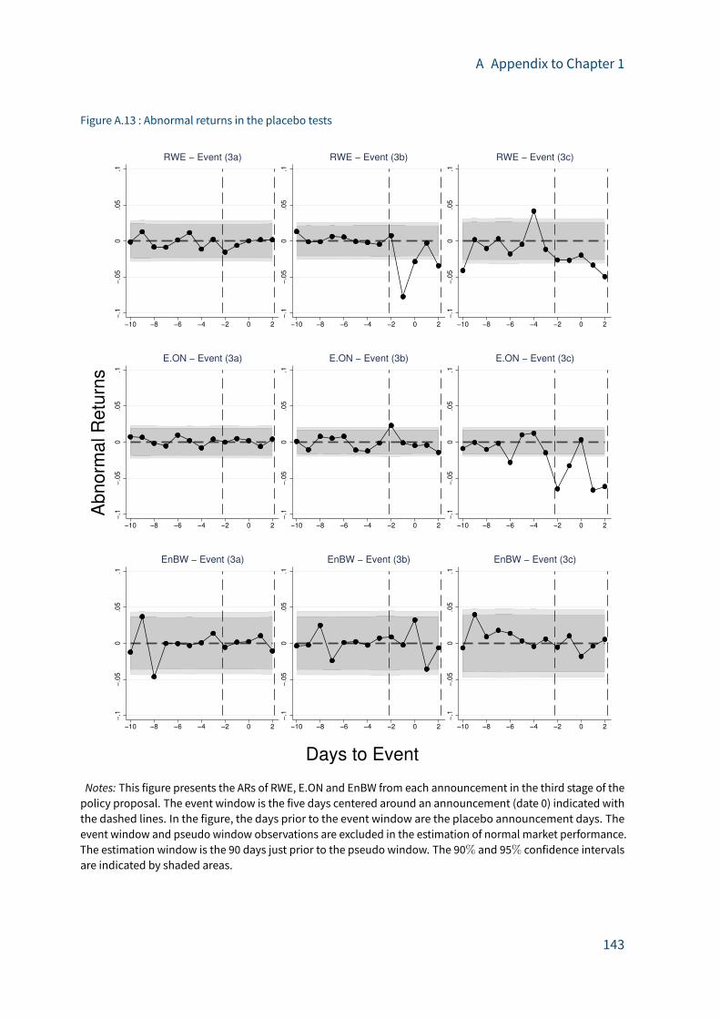
A Appendix to Chapter 1
Figure A.13 : Abnormal returns in the placebo tests−
.1−
.05
0.0
5.1
−10 −8 −6 −4 −2 0 2
RWE − Event (3a)
−.1
−.0
50
.05
.1
−10 −8 −6 −4 −2 0 2
RWE − Event (3b)
−.1
−.0
50
.05
.1
−10 −8 −6 −4 −2 0 2
RWE − Event (3c)
−.1
−.0
50
.05
.1
−10 −8 −6 −4 −2 0 2
E.ON − Event (3a)
−.1
−.0
50
.05
.1
−10 −8 −6 −4 −2 0 2
E.ON − Event (3b)
−.1
−.0
50
.05
.1
−10 −8 −6 −4 −2 0 2
E.ON − Event (3c)
−.1
−.0
50
.05
.1
−10 −8 −6 −4 −2 0 2
EnBW − Event (3a)
−.1
−.0
50
.05
.1
−10 −8 −6 −4 −2 0 2
EnBW − Event (3b)
−.1
−.0
50
.05
.1
−10 −8 −6 −4 −2 0 2
EnBW − Event (3c)
Abnorm
al R
etu
rns
Days to Event
Notes: This figure presents the ARs of RWE, E.ON and EnBW from each announcement in the third stage of thepolicy proposal. The event window is the five days centered around an announcement (date 0) indicated withthe dashed lines. In the figure, the days prior to the event window are the placebo announcement days. Theevent window and pseudo window observations are excluded in the estimation of normal market performance.The estimation window is the 90 days just prior to the pseudo window. The 90% and 95% confidence intervalsare indicated by shaded areas.
143
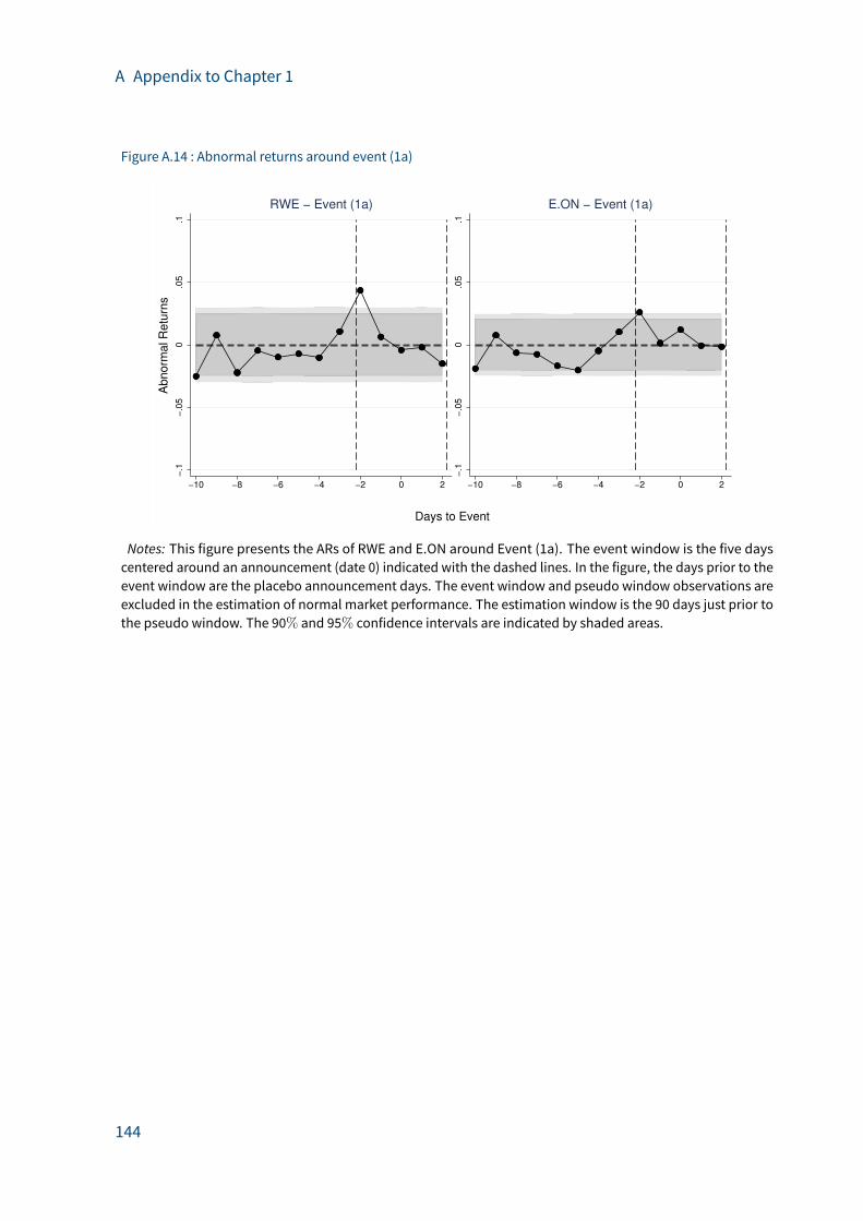
A Appendix to Chapter 1
Figure A.14 : Abnormal returns around event (1a)−
.1−
.05
0.0
5.1
−10 −8 −6 −4 −2 0 2
RWE − Event (1a)
−.1
−.0
50
.05
.1
−10 −8 −6 −4 −2 0 2
E.ON − Event (1a)
Ab
no
rma
l R
etu
rns
Days to Event
Notes: This figure presents the ARs of RWE and E.ON around Event (1a). The event window is the five dayscentered around an announcement (date 0) indicated with the dashed lines. In the figure, the days prior to theevent window are the placebo announcement days. The event window and pseudo window observations areexcluded in the estimation of normal market performance. The estimation window is the 90 days just prior tothe pseudo window. The 90% and 95% confidence intervals are indicated by shaded areas.
144
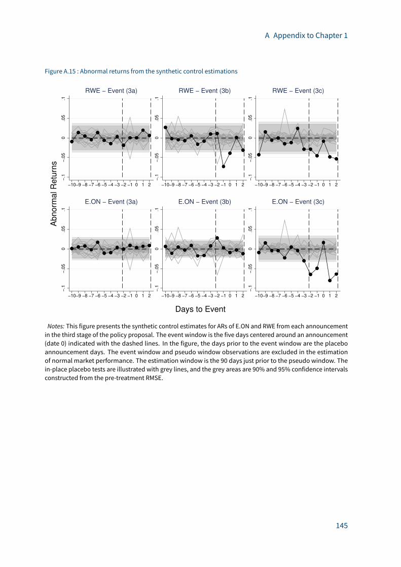
A Appendix to Chapter 1
Figure A.15 : Abnormal returns from the synthetic control estimations−
.1−
.05
0.0
5.1
−10−9 −8 −7 −6 −5 −4 −3 −2 −1 0 1 2
RWE − Event (3a)
−.1
−.0
50
.05
.1
−10−9 −8 −7 −6 −5 −4 −3 −2 −1 0 1 2
RWE − Event (3b)
−.1
−.0
50
.05
.1
−10−9 −8 −7 −6 −5 −4 −3 −2 −1 0 1 2
RWE − Event (3c)
−.1
−.0
50
.05
.1
−10−9 −8 −7 −6 −5 −4 −3 −2 −1 0 1 2
E.ON − Event (3a)
−.1
−.0
50
.05
.1
−10−9 −8 −7 −6 −5 −4 −3 −2 −1 0 1 2
E.ON − Event (3b)
−.1
−.0
50
.05
.1
−10−9 −8 −7 −6 −5 −4 −3 −2 −1 0 1 2
E.ON − Event (3c)
Ab
norm
al R
etu
rns
Days to Event
Notes: This figure presents the synthetic control estimates for ARs of E.ON and RWE from each announcementin the third stage of the policy proposal. The event window is the five days centered around an announcement(date 0) indicated with the dashed lines. In the figure, the days prior to the event window are the placeboannouncement days. The event window and pseudo window observations are excluded in the estimationof normal market performance. The estimation window is the 90 days just prior to the pseudo window. Thein-place placebo tests are illustrated with grey lines, and the grey areas are 90% and 95% confidence intervalsconstructed from the pre-treatment RMSE.
145
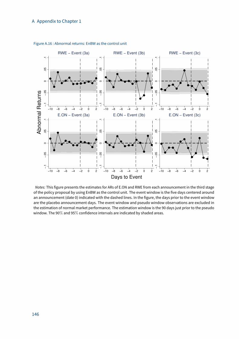
A Appendix to Chapter 1
Figure A.16 : Abnormal returns: EnBW as the control unit−
.1−
.05
0.0
5.1
−10 −8 −6 −4 −2 0 2
RWE − Event (3a)
−.1
−.0
50
.05
.1
−10 −8 −6 −4 −2 0 2
RWE − Event (3b)
−.1
−.0
50
.05
.1
−10 −8 −6 −4 −2 0 2
RWE − Event (3c)
−.1
−.0
50
.05
.1
−10 −8 −6 −4 −2 0 2
E.ON − Event (3a)
−.1
−.0
50
.05
.1
−10 −8 −6 −4 −2 0 2
E.ON − Event (3b)
−.1
−.0
50
.05
.1
−10 −8 −6 −4 −2 0 2
E.ON − Event (3c)
Abn
orm
al R
etu
rns
Days to Event
Notes: This figure presents the estimates for ARs of E.ON and RWE from each announcement in the third stageof the policy proposal by using EnBW as the control unit. The event window is the five days centered aroundan announcement (date 0) indicated with the dashed lines. In the figure, the days prior to the event windoware the placebo announcement days. The event window and pseudo window observations are excluded inthe estimation of normal market performance. The estimation window is the 90 days just prior to the pseudowindow. The 90% and 95% confidence intervals are indicated by shaded areas.
146
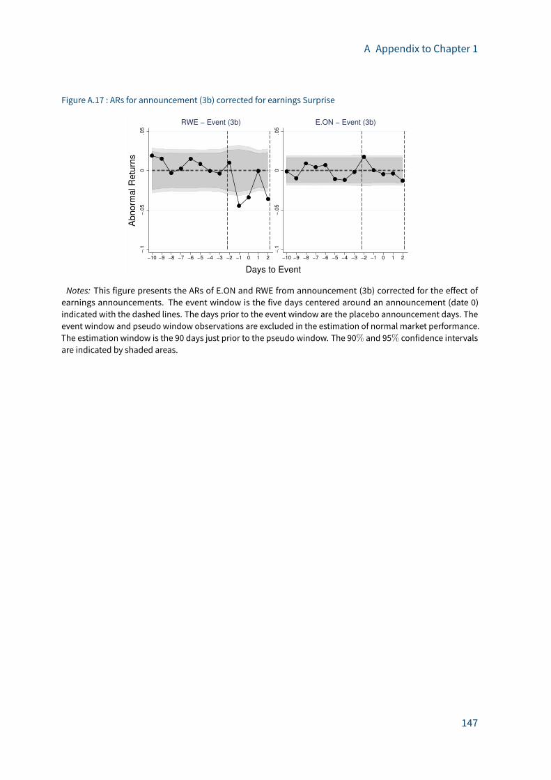
A Appendix to Chapter 1
Figure A.17 : ARs for announcement (3b) corrected for earnings Surprise
−.1
−.0
50
.05
−10 −9 −8 −7 −6 −5 −4 −3 −2 −1 0 1 2
RWE − Event (3b)
−.1
−.0
50
.05
−10 −9 −8 −7 −6 −5 −4 −3 −2 −1 0 1 2
E.ON − Event (3b)
Ab
no
rma
l R
etu
rns
Days to Event
Notes: This figure presents the ARs of E.ON and RWE from announcement (3b) corrected for the e�ect ofearnings announcements. The event window is the five days centered around an announcement (date 0)indicated with the dashed lines. The days prior to the event window are the placebo announcement days. Theevent window and pseudo window observations are excluded in the estimation of normal market performance.The estimation window is the 90 days just prior to the pseudo window. The 90% and 95% confidence intervalsare indicated by shaded areas.
147


B Appendix to Chapter 2
B.1 Patent example and patent classi�cation codes
Figure B.1 : Patent example
149
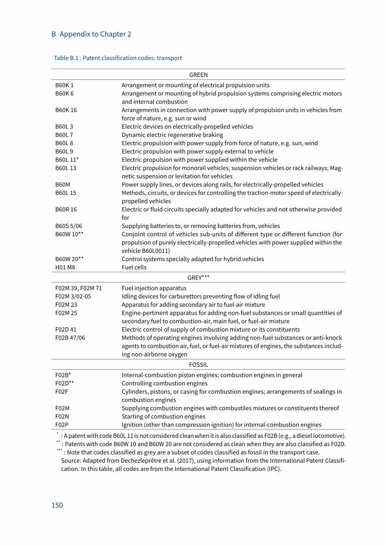
B Appendix to Chapter 2
Table B.1 : Patent classification codes: transport
GREEN
B60K 1 Arrangement or mounting of electrical propulsion unitsB60K 6 Arrangement or mounting of hybrid propulsion systems comprising electric motors
and internal combustionB60K 16 Arrangements in connection with power supply of propulsion units in vehicles from
force of nature, e.g. sun or windB60L 3 Electric devices on electrically-propelled vehiclesB60L 7 Dynamic electric regenerative brakingB60L 8 Electric propulsion with power supply from force of nature, e.g. sun, windB60L 9 Electric propulsion with power supply external to vehicleB60L 11* Electric propulsion with power supplied within the vehicleB60L 13 Electric propulsion for monorail vehicles, suspension vehicles or rack railways; Mag-
netic suspension or levitation for vehiclesB60M Power supply lines, or devices along rails, for electrically-propelled vehiclesB60L 15 Methods, circuits, or devices for controlling the traction-motor speed of electrically-
propelled vehiclesB60R 16 Electric or fluid circuits specially adapted for vehicles and not otherwise provided
forB60S 5/06 Supplying batteries to, or removing batteries from, vehiclesB60W 10** Conjoint control of vehicles sub-units of di�erent type or di�erent function (for
propulsion of purely electrically-propelled vehicles with power supplied within thevehicle B60L0011)
B60W 20** Control systems specially adapted for hybrid vehiclesH01 M8 Fuel cells
GREY***
F02M 39, F02M 71 Fuel injection apparatusF02M 3/02-05 Idling devices for carburettors preventing flow of idling fuelF02M 23 Apparatus for adding secondary air to fuel-air mixtureF02M 25 Engine-pertinent apparatus for adding non-fuel substances or small quantities of
secondary fuel to combustion-air, main fuel, or fuel-air mixtureF02D 41 Electric control of supply of combustion mixture or its constituentsF02B 47/06 Methods of operating engines involving adding non-fuel substances or anti-knock
agents to combustion air, fuel, or fuel-air mixtures of engines, the substances includ-ing non-airborne oxygen
FOSSIL
F02B* Internal-combustion piston engines; combustion engines in generalF02D** Controlling combustion enginesF02F Cylinders, pistons, or casing for combustion engines; arrangements of sealings in
combustion enginesF02M Supplying combustion engines with combustiles mixtures or constituents thereofF02N Starting of combustion enginesF02P Ignition (other than compression ignition) for internal-combustion engines* : A patentwith codeB60L 11 is not considered cleanwhen it is also classified as F02B (e.g., a diesel locomotive).** : Patents with code B60W 10 and B60W 20 are not considered as clean when they are also classified as F02D.*** : Note that codes classified as grey are a subset of codes classified as fossil in the transport case.Source: Adapted from Dechezleprêtre et al. (2017), using information from the International Patent Classifi-cation. In this table, all codes are from the International Patent Classification (IPC).
150

B Appendix to Chapter 2
Table B.2 : Patent classification codes: energy
GREEN
Y02E 10 Energy generation through renewable energy sourcesY02E 30 Energy generation of nuclear originE02B 8/08 Tide or wave power plantsF03B 13/10-26 Submerged units incorporating electric generators or motors characterized by using
wave or tide energyF03D WindmotorsF03G 4 Devices for producing mechanical power from geothermal energyF03G 6 Devices for producing mechanical power from solar energyF03G 7/05 Ocean thermal energy conversionF24J 2 Use of solar heatF24J 3 Other production or use of heat, not derived from combustionF24S Solar heat collectors; solar heat systemsF24T Geothermal collectors; geothermal systemsF26B 3/28 Drying solid materials or objects by processes involving the application of heat by
radiation, e.g. from the sun
GREY
Y02 E20 Combustion technologies with mitigation potentialY02 E50 Technologies for the production of fuel of non-fossil origin
FOSSIL
C10 G1 Production of liquid hydrocarbonmixtures from oil-shale, oil-sand, or non-meltingsolid carbonaceous or similar materials, e.g. wood, coal
C10 L1 FuelC10 J Production of fuel gases by carburetting air or other gasesF01 K Steam engine plants; steam accumulators; engine plants not otherwise provided
for; engines using special working fluids or cyclesF02 C Gas-turbine plants; air intakes for jet-propulsion plants; controlling fuel supply in
air-breathing jet-propulsion plantsF22 Steam generationF23 Combustion apparatus; combustion processesF27 Furnaces; kilns; ovens; retorts
Source: Adapted from Dechezleprêtre et al. (2017), using information from the International Patent Classifi-cation and Cooperative Patent Classification.In this table, the patent classes starting with Y are from the Cooperative Patent Classification (CPC), all othercodes are from the International Patent Classification (IPC).
151

B Appendix to Chapter 2
B.2 Mapping of investor types
Table B.3 provides an overview of themapping of shareholder types. The shareholders are
identified by their own BvD ID (if available). In order to classify them into di�erent shareholder
types, both their NACE code and the “entity type” asigned by BvD are used. Each of the
classifications have their own advantages and disadvantages. NACE codes generally allow for
a good distinction between private financial services institutions, such as banks, investment
funds, or insuranceandpension funds. However, outsideof the financial services classification,
NACE codes become less useful: many foundations, private funds or even cooperative banks
are classified as “Activities of membership organizations”. The shareholder types provided by
BvD, on the other hand, identify these institutions more clearly. Moreover, they are generally
useful to distinguish between individuals and institutional investors, and to di�erentiate
between government investors and private ones. Within private investment organizations, the
attribution of types in the BvD classification seems somewhat arbitrary (e.g. pension funds
are sometimes coded as “insurance companies”, and BlackRock is labelled “Bank”). Therefore,
the financial sector classification follows, and slightly adapts, the approach from Battiston
et al. (2017):
– The Orbis classification is used in case of “Government” and “Foundation”.
– In all other cases, the NACE classification is used, if it is available and if it is equal tosome financial services-related sector (for the mapping, see Table B.3).
– If no NACE code is available or if it is not related to financial services, the Orbis classifica-tion is used (for the mapping, see Table B.3).
– Investors which do not belong to the institutional ownership category are dropped fromthe analysis:
• In case the Orbis classification lists them as “Industrial Company”, “self-owned”, or
“One or more known individuals or families”, observations are excluded.
• In case the Orbis classification lists them as “Other unnamed private shareholders” or
“Other unnamed shareholders”, they are excluded if there is no NACE code available
(these o�en appear to be unclassified funds or investment vehicles).
152
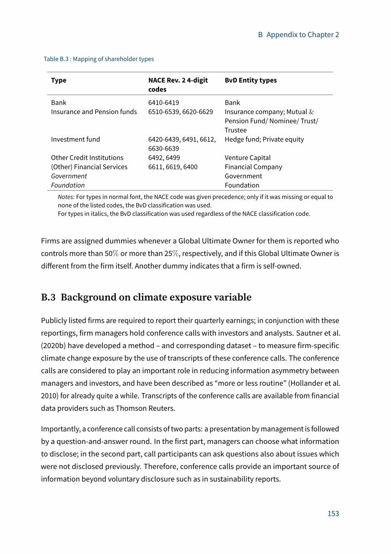
B Appendix to Chapter 2
Table B.3 : Mapping of shareholder types
Type NACE Rev. 2 4-digitcodes
BvD Entity types
Bank 6410-6419 BankInsurance and Pension funds 6510-6539, 6620-6629 Insurance company; Mutual&
Pension Fund/ Nominee/ Trust/Trustee
Investment fund 6420-6439, 6491, 6612,6630-6639
Hedge fund; Private equity
Other Credit Institutions 6492, 6499 Venture Capital(Other) Financial Services 6611, 6619, 6400 Financial CompanyGovernment GovernmentFoundation Foundation
Notes: For types in normal font, the NACE code was given precedence; only if it was missing or equal tonone of the listed codes, the BvD classification was used.For types in italics, the BvD classification was used regardless of the NACE classification code.
Firms are assigned dummies whenever a Global Ultimate Owner for them is reported who
controls more than 50% or more than 25%, respectively, and if this Global Ultimate Owner is
di�erent from the firm itself. Another dummy indicates that a firm is self-owned.
B.3 Background on climate exposure variable
Publicly listed firms are required to report their quarterly earnings; in conjunction with these
reportings, firmmanagers hold conference calls with investors and analysts. Sautner et al.
(2020b) have developed a method – and corresponding dataset – to measure firm-specific
climate change exposure by the use of transcripts of these conference calls. The conference
calls are considered to play an important role in reducing information asymmetry between
managers and investors, and have been described as “more or less routine” (Hollander et al.
2010) for already quite a while. Transcripts of the conference calls are available from financial
data providers such as Thomson Reuters.
Importantly, a conference call consists of twoparts: a presentationbymanagement is followed
by a question-and-answer round. In the first part, managers can choose what information
to disclose; in the second part, call participants can ask questions also about issues which
were not disclosed previously. Therefore, conference calls provide an important source of
information beyond voluntary disclosure such as in sustainability reports.
153
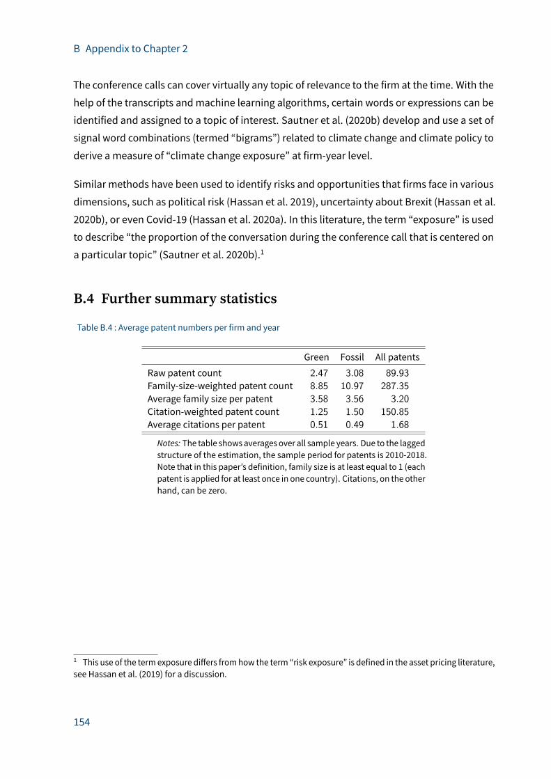
B Appendix to Chapter 2
The conference calls can cover virtually any topic of relevance to the firm at the time. With the
help of the transcripts andmachine learning algorithms, certain words or expressions can be
identified and assigned to a topic of interest. Sautner et al. (2020b) develop and use a set of
signal word combinations (termed “bigrams”) related to climate change and climate policy to
derive a measure of “climate change exposure” at firm-year level.
Similar methods have been used to identify risks and opportunities that firms face in various
dimensions, such as political risk (Hassan et al. 2019), uncertainty about Brexit (Hassan et al.
2020b), or even Covid-19 (Hassan et al. 2020a). In this literature, the term “exposure” is used
to describe “the proportion of the conversation during the conference call that is centered on
a particular topic” (Sautner et al. 2020b).1
B.4 Further summary statistics
Table B.4 : Average patent numbers per firm and year
Green Fossil All patentsRaw patent count 2.47 3.08 89.93
Family-size-weighted patent count 8.85 10.97 287.35
Average family size per patent 3.58 3.56 3.20
Citation-weighted patent count 1.25 1.50 150.85
Average citations per patent 0.51 0.49 1.68
Notes: The table showsaverages over all sample years. Due to the laggedstructure of the estimation, the sample period for patents is 2010-2018.Note that in this paper’s definition, family size is at least equal to 1 (eachpatent is applied for at least once in one country). Citations, on the otherhand, can be zero.
1 This use of the termexposure di�ers fromhow the term “risk exposure” is defined in the asset pricing literature,see Hassan et al. (2019) for a discussion.
154
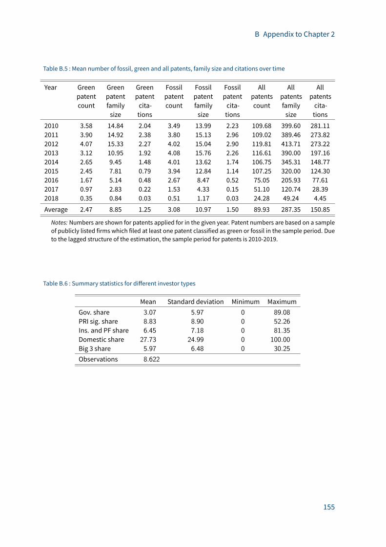
B Appendix to Chapter 2
Table B.5 : Mean number of fossil, green and all patents, family size and citations over time
Year Greenpatentcount
Greenpatentfamilysize
Greenpatentcita-tions
Fossilpatentcount
Fossilpatentfamilysize
Fossilpatentcita-tions
Allpatentscount
Allpatentsfamilysize
Allpatentscita-tions
2010 3.58 14.84 2.04 3.49 13.99 2.23 109.68 399.60 281.112011 3.90 14.92 2.38 3.80 15.13 2.96 109.02 389.46 273.822012 4.07 15.33 2.27 4.02 15.04 2.90 119.81 413.71 273.222013 3.12 10.95 1.92 4.08 15.76 2.26 116.61 390.00 197.162014 2.65 9.45 1.48 4.01 13.62 1.74 106.75 345.31 148.772015 2.45 7.81 0.79 3.94 12.84 1.14 107.25 320.00 124.302016 1.67 5.14 0.48 2.67 8.47 0.52 75.05 205.93 77.612017 0.97 2.83 0.22 1.53 4.33 0.15 51.10 120.74 28.392018 0.35 0.84 0.03 0.51 1.17 0.03 24.28 49.24 4.45Average 2.47 8.85 1.25 3.08 10.97 1.50 89.93 287.35 150.85
Notes: Numbers are shown for patents applied for in the given year. Patent numbers are based on a sampleof publicly listed firms which filed at least one patent classified as green or fossil in the sample period. Dueto the lagged structure of the estimation, the sample period for patents is 2010-2019.
Table B.6 : Summary statistics for di�erent investor types
Mean Standard deviation Minimum MaximumGov. share 3.07 5.97 0 89.08
PRI sig. share 8.83 8.90 0 52.26
Ins. and PF share 6.45 7.18 0 81.35
Domestic share 27.73 24.99 0 100.00
Big 3 share 5.97 6.48 0 30.25
Observations 8.622
155
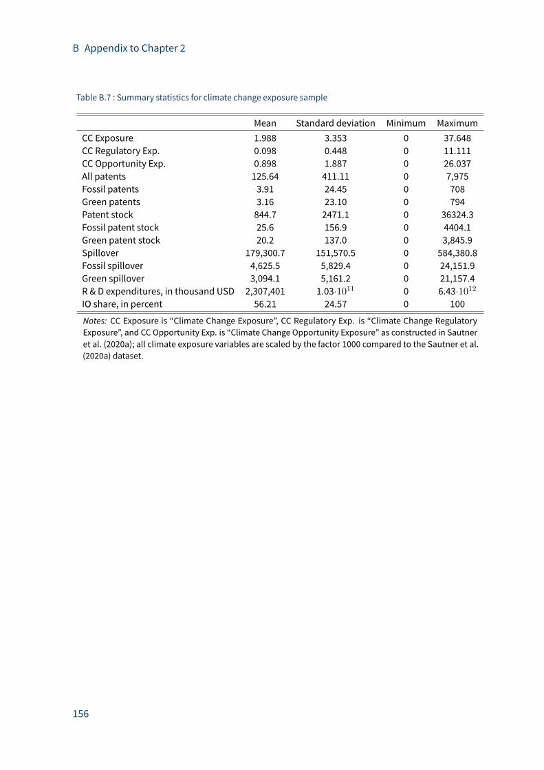
B Appendix to Chapter 2
Table B.7 : Summary statistics for climate change exposure sample
Mean Standard deviation Minimum MaximumCC Exposure 1.988 3.353 0 37.648CC Regulatory Exp. 0.098 0.448 0 11.111CC Opportunity Exp. 0.898 1.887 0 26.037All patents 125.64 411.11 0 7,975Fossil patents 3.91 24.45 0 708Green patents 3.16 23.10 0 794Patent stock 844.7 2471.1 0 36324.3Fossil patent stock 25.6 156.9 0 4404.1Green patent stock 20.2 137.0 0 3,845.9Spillover 179,300.7 151,570.5 0 584,380.8Fossil spillover 4,625.5 5,829.4 0 24,151.9Green spillover 3,094.1 5,161.2 0 21,157.4R & D expenditures, in thousand USD 2,307,401 1.03·1011 0 6.43·1012IO share, in percent 56.21 24.57 0 100
Notes: CC Exposure is “Climate Change Exposure”, CC Regulatory Exp. is “Climate Change RegulatoryExposure”, and CC Opportunity Exp. is “Climate Change Opportunity Exposure” as constructed in Sautneret al. (2020a); all climate exposure variables are scaled by the factor 1000 compared to the Sautner et al.(2020a) dataset.
156

B Appendix to Chapter 2
B.5 Further estimation results
Table B.8 : Family size and grey patents
(1) (2) (3)Dep. var. Green family size Fossil family size Grey patents
L.IO share 0.000346 -0.00364 -0.00489(0.0391) (0.0276) (0.140)
L.Own stock fossil, FS 0.105∗∗∗ 0.887∗∗∗
(0.0385) (0.0858)L.Own stock green, FS 1.034∗∗∗ 0.0332
(0.0838) (0.0672)L.Green spillover, FS 0.0104 -0.0205
(0.598) (0.417)L.Fossil spillover, FS -0.0304 0.00764
(0.598) (0.414)L.R and D exp. 0.128 0.165 0.330
(0.166) (0.123) (0.602)L.Own stock fossil 0.378
(0.246)L.Own stock green -0.271
(0.329)L.Own stock grey 1.896∗∗∗
(0.231)L.Green spillover -0.153
(2.935)L.Fossil spillover -0.730
(2.328)L.Grey spillover 0.810
(0.756)
Observations 8622 8622 8622
Notes: All columns: Poisson control function estimations (first stage not shown). Robust standard errors inparentheses. Knowledge stocks, spillovers and R&D expenditures are in logs. Estimation period is 2009-2018.All regressions include year fixed e�ects and firm fixed e�ects using the BGVRmethod. Significance levels areindicated as ∗ p < 0.1, ∗∗ p < 0.05, ∗∗∗ p < 0.01.
157

B Appendix to Chapter 2
Table B.9 : Ownership concentration and two-year lag
(1) (2) (3) (4)Dep. var. Green patents Fossil patents Green patents Fossil patents
L.Top 5 share -0.0629 -0.0282(0.148) (0.102)
L2.IO share 0.0673 -0.00383(0.0705) (0.0414)
L.Own stock fossil 0.101∗ 1.283∗∗∗ 0.170∗∗ 1.295∗∗∗
(0.0536) (0.0780) (0.0768) (0.124)L.Own stock green 1.435∗∗∗ 0.00734 1.575∗∗∗ -0.00861
(0.0715) (0.0502) (0.154) (0.128)L.Green spillover 0.0742 -0.00195 1.488 -0.126
(0.0834) (0.0749) (1.502) (0.867)L.Fossil spillover -0.0590 -0.0150 -1.463 0.119
(0.0813) (0.0742) (1.503) (0.867)L.R and D exp. 0.0763 0.123∗∗ -0.170 0.162
(0.0825) (0.0624) (0.309) (0.189)
Observations 8622 8622 7345 7345
Notes: All columns: Poisson control function estimations (first stage not shown). Robust standard errors inparentheses. Knowledge stocks, spillovers and R&D expenditures are in logs. Estimation period is 2009-2018.All regressions include year fixed e�ects and firm fixed e�ects using the BGVRmethod. Significance levels areindicated as ∗ p < 0.1, ∗∗ p < 0.05, ∗∗∗ p < 0.01.
158

B Appendix to Chapter 2
Table B.10 : Special investor types and green patenting, full table
(1) (2) (3) (4) (5)
L.Gov. share 0.0342(0.0882)
L.PRI sig. share 0.0343(0.0796)
L.Ins.& pens. fd. share -0.121(0.298)
L.Domestic owner share -0.0210(0.0505)
L.Big 3 share 0.0257(0.0610)
L.Own stock green 1.431∗∗∗ 1.452∗∗∗ 1.445∗∗∗ 1.421∗∗∗ 1.444∗∗∗
(0.0720) (0.0851) (0.0908) (0.0769) (0.0775)L.Own stock fossil 0.110∗∗ 0.113∗∗∗ 0.0909 0.0850 0.111∗∗
(0.0437) (0.0425) (0.0793) (0.0851) (0.0435)L.Green spillover 0.0777 0.259 -0.270 -0.251 0.182
(0.0805) (0.416) (0.877) (0.807) (0.246)L.Fossil spillover -0.0294 -0.235 0.320 0.322 -0.160
(0.0954) (0.434) (0.923) (0.902) (0.268)L.R and D exp. 0.0997∗∗∗ 0.0712 0.161 0.176 0.0755
(0.0356) (0.0937) (0.119) (0.162) (0.0874)
Observations 8622 8622 8622 8622 8622
Notes: Dependent variable: Green patents. All columns: Poisson control function estimations (first stage notshown). Robust standard errors in parentheses. Knowledge stocks, spillovers and R&D expenditures are inlogs. Estimation period is 2009-2018. All regressions include year fixed e�ects and firm fixed e�ects using theBGVRmethod. Significance levels are indicated as ∗ p < 0.1, ∗∗ p < 0.05, ∗∗∗ p < 0.01.
159
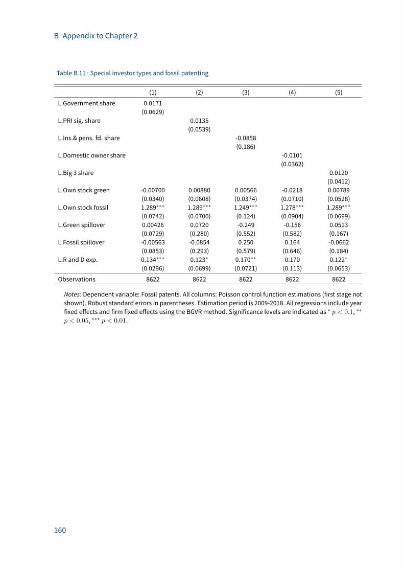
B Appendix to Chapter 2
Table B.11 : Special investor types and fossil patenting
(1) (2) (3) (4) (5)
L.Government share 0.0171(0.0629)
L.PRI sig. share 0.0135(0.0539)
L.Ins.& pens. fd. share -0.0858(0.186)
L.Domestic owner share -0.0101(0.0362)
L.Big 3 share 0.0120(0.0412)
L.Own stock green -0.00700 0.00880 0.00566 -0.0218 0.00789(0.0340) (0.0608) (0.0374) (0.0710) (0.0528)
L.Own stock fossil 1.289∗∗∗ 1.289∗∗∗ 1.249∗∗∗ 1.278∗∗∗ 1.289∗∗∗
(0.0742) (0.0700) (0.124) (0.0904) (0.0699)L.Green spillover 0.00426 0.0720 -0.249 -0.156 0.0513
(0.0729) (0.280) (0.552) (0.582) (0.167)L.Fossil spillover -0.00563 -0.0854 0.250 0.164 -0.0662
(0.0853) (0.293) (0.579) (0.646) (0.184)L.R and D exp. 0.134∗∗∗ 0.123∗ 0.170∗∗ 0.170 0.122∗
(0.0296) (0.0699) (0.0721) (0.113) (0.0653)
Observations 8622 8622 8622 8622 8622
Notes: Dependent variable: Fossil patents. All columns: Poisson control function estimations (first stage notshown). Robust standard errors in parentheses. Estimation period is 2009-2018. All regressions include yearfixed e�ects and firm fixed e�ects using the BGVRmethod. Significance levels are indicated as ∗ p < 0.1, ∗∗
p < 0.05, ∗∗∗ p < 0.01.
160

B Appendix to Chapter 2
Table B.12 : Institutional investors and totel patents, full table
(1) (2) (3) (4) (5) (6)Model Poisson Poisson Poisson Poisson Poisson Neg. bin.Dep. var. Patents Patents Patents Family size Citations PatentsL.IO share 0.0114∗∗∗ 0.0114∗∗ 0.0110∗ 0.0129∗∗ -0.0258 0.00671∗∗
(0.00348) (0.00481) (0.00603) (0.00624) (0.0177) (0.00310)L.Own patent stock 1.274∗∗∗ 1.274∗∗∗ 1.270∗∗∗ 1.483∗∗∗
(0.0374) (0.0313) (0.0370) (0.0340)L.Own patent stock, FS 1.109∗∗∗
(0.0540)L.Own patent stock, cit. 1.318∗∗∗
(0.0758)L.Total spillover -0.0174∗ -0.0174 -0.0154 -0.0167
(0.00902) (0.0161) (0.0172) (0.0104)L.Total spillover, FS -0.00957
(0.0224)L.Total spillover, cit. 0.0989
(0.0633)L.Tobin’s Q 0.0257
(0.0276)L.R and D exp. 0.0132 0.0132 0.0179 0.0447 0.128∗∗ 0.0358
(0.0277) (0.0374) (0.0436) (0.0467) (0.0610) (0.0228)Clustered SEs no yes yes yes yes yesAdd. control no no yes no no noObservations 8622 8622 8040 8622 8622 8622
Notes: All estimations use a control function approach (first stage not shown). “Add. control” refers to theinclusion of Tobin’s q as an additional control variable. Robust standard errors in parentheses. In the Poissoncontrol function estimations starting in column 2, standard errors are two-way clustered at the 4-digit NACEcode and country level. In the negative binomial control function estimation, standard errors are clusteredat the 4-digit NACE code level. Knowledge stocks, spillovers and R&D expenditures are in logs. Estimationperiod is 2009-2018. All regressions include year fixed e�ects, and firm fixed e�ects using the BGVRmethod.Significance levels are indicated as ∗ p < 0.1, ∗∗ p < 0.05, ∗∗∗ p < 0.01.
161
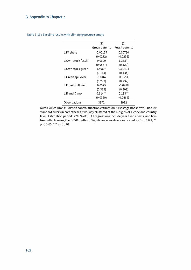
B Appendix to Chapter 2
Table B.13 : Baseline results with climate exposure sample
(1) (2)Green patents Fossil patents
L.IO share -0.00157 0.00760(0.0272) (0.0236)
L.Own stock fossil 0.0609 1.335∗∗
(0.0567) (0.120)L.Own stock green 1.496∗∗ 0.00494
(0.114) (0.134)L.Green spillover -0.0467 0.0551
(0.293) (0.237)L.Fossil spillover 0.0525 -0.0488
(0.363) (0.309)L.R and D exp. 0.114∗∗ 0.133∗∗
(0.0399) (0.0469)Observations 3972 3972
Notes: All columns: Poisson control function estimation (first stage not shown). Robuststandard errors in parentheses, two-way clustered at the 4-digit NACE code and countrylevel. Estimation period is 2009-2018. All regressions include year fixed e�ects, and firmfixed e�ects using the BGVR method. Significance levels are indicated as ∗ p < 0.1, ∗∗
p < 0.05, ∗∗∗ p < 0.01.
162

C Appendix to Chapter 3
C.1 Sectors
Table C.1 : Sector description and numbers
Sector number Sector description
1 Agriculture, forestry and fishing2 Mining and quarrying3 Food, beverages, textiles, leather4 Wood, paper, publishing, broadcasting, arts, entertainment, recreation5 Coke and refined petroleum products6 Chemicals and pharmaceuticals7 Rubber, plastic and glass products and ceramics8 Metals & metal products, machinery & equipment, and other products9 Water supply, sewerage, waste management and remediation10 Electricity from coal11 Electricity from gas12 Electricity from hydro13 Electricity fromwind14 Electricity from biomass and waste15 Electricity from solar (PV and thermal)16 Electricity nec (incl. nuclear, oil); steam & hot water17 Transmission of electricity18 Distribution and trade of electricity19 Manufacture of gas; distribution of gaseous fuels throughmains20 Construction21 Wholesale and retail trade, repairs, including motor vehicles22 Hotels and restaurants23 Transport, warehousing, post and telecommunications24 Financial and insurance services25 Real estate activities26 Rental & leasing; other business services27 Computer programming and information service28 Scientific research & development29 Public administration & defense, social security30 Education31 Human health and social work activities32 Activities of membership organizations and other personal service activities
163

C Appendix to Chapter 3
Table C.2 : Available regional gross value added values
Aggregatedsector
CorrespondingCPA classifications
Sector description
A 1-3 Agriculture, forestry and fishingB-E 5-39 Industry excluding constructionC 10-33 ManufacturingB, D, E 5-9, 35-39 Industry excluding construction andmanufacturing. B: Mining and
quarrying; D: Electricity, gas, steam and air conditioning supply;E: Water supply; sewerage, waste management and remediationactivities
F 41-43 ConstructionG-J 45-63 G: Trade, repair of motor vehicles; H: Transportation and storage; I:
accommodation and food services; J: Information and communica-tion
K-N 64-82 K: Financial and insurance activities; L: real estate activities; M: Pro-fessional, scientific and technical activities; N: Administrative andsupport service activities
O-T 84-98 O: Public administration and defense, social security; P: Education;Q: Health and social work; R: Arts, entertainment and recreation; S:Other service activities; T: Activities of households as employers
164

C Appendix to Chapter 3
C.2 Details on disaggregation of capital stocks
For the electricity-producing technologies, data on installed capacity are from ENTSO-E
(2017b) and (for renewables) IRENA (2016a). Data on installation costs were combined (and
sometimes averaged) from various sources (Nitsch et al. 2012; AEE 2012; Breyer et al. 2013;
Dumont and Keuneke 2011; Blesl et al. 2012; Kost et al. 2013; Hirschl et al. 2015; Hobohm and
Mellahn 2010; Peter et al. 2013; Photovoltaik-Guide 2017; Sachverständigenrat für Umweltfra-
gen 2011; Pahle et al. 2012; Bickel et al. 2012).
Data on the length of electricity transmission lines were obtained from ENTSO-E (2017a).
Information from ACER (2015) and ICF Consulting (2003) was combined to derive installation
costs per kilometer. For electricity distribution, data on the length of distribution networks
come from Vaillancourt (2012), and data on the investment costs are from Deutsche Energie-
Agentur (2012).
In the heat sector, Eurostat (2016b) provides information on the amount (energy content) of
derived heat available for final consumption. The data on investment cost per heat demand
came from Grözinger et al. (2013). Finally, data on gas distribution networks was obtained
from Eurogas (2008), while the cost per km is an estimate based on press reports on costs of
the German distribution network at di�erent pressure levels, scaled by the shares of these
pressure levels.
165
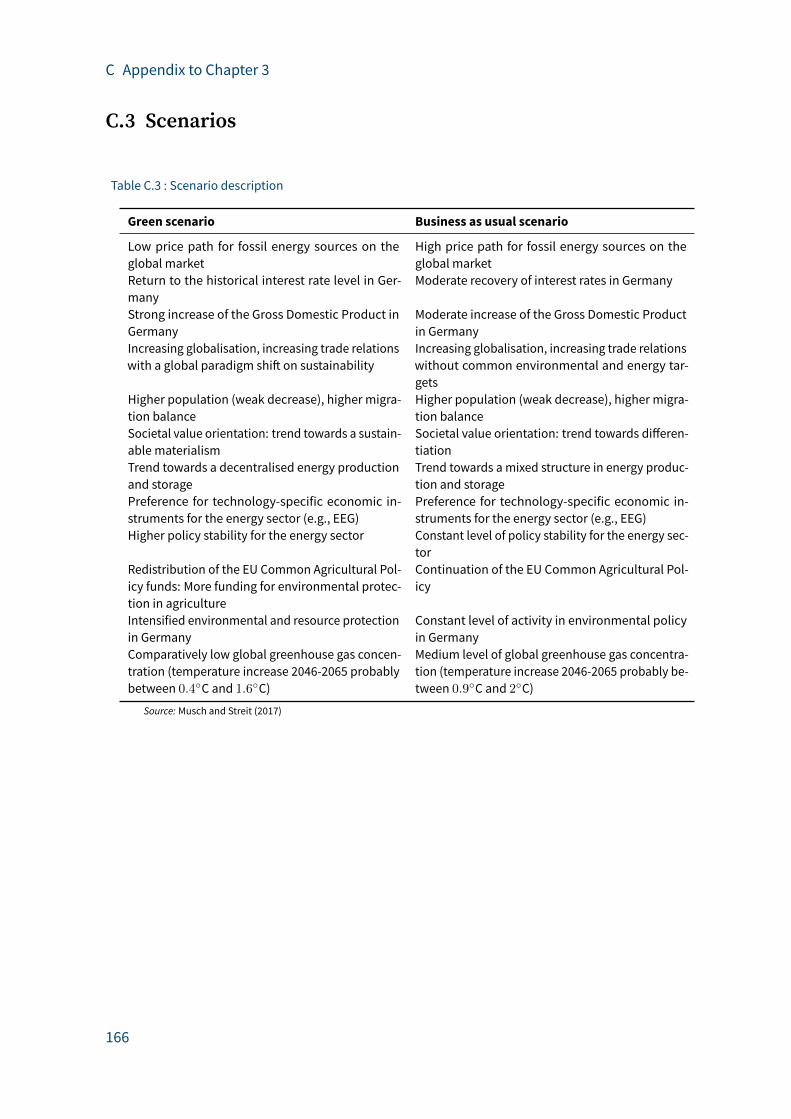
C Appendix to Chapter 3
C.3 Scenarios
Table C.3 : Scenario description
Green scenario Business as usual scenario
Low price path for fossil energy sources on theglobal market
High price path for fossil energy sources on theglobal market
Return to the historical interest rate level in Ger-many
Moderate recovery of interest rates in Germany
Strong increase of the Gross Domestic Product inGermany
Moderate increase of the Gross Domestic Productin Germany
Increasing globalisation, increasing trade relationswith a global paradigm shi� on sustainability
Increasing globalisation, increasing trade relationswithout common environmental and energy tar-gets
Higher population (weak decrease), higher migra-tion balance
Higher population (weak decrease), higher migra-tion balance
Societal value orientation: trend towards a sustain-able materialism
Societal value orientation: trend towards di�eren-tiation
Trend towards a decentralised energy productionand storage
Trend towards a mixed structure in energy produc-tion and storage
Preference for technology-specific economic in-struments for the energy sector (e.g., EEG)
Preference for technology-specific economic in-struments for the energy sector (e.g., EEG)
Higher policy stability for the energy sector Constant level of policy stability for the energy sec-tor
Redistribution of the EU Common Agricultural Pol-icy funds: More funding for environmental protec-tion in agriculture
Continuation of the EU Common Agricultural Pol-icy
Intensified environmental and resource protectionin Germany
Constant level of activity in environmental policyin Germany
Comparatively low global greenhouse gas concen-tration (temperature increase 2046-2065 probablybetween 0.4◦C and 1.6◦C)
Medium level of global greenhouse gas concentra-tion (temperature increase 2046-2065 probably be-tween 0.9◦C and 2◦C)
Source: Musch and Streit (2017)
166

C Appendix to Chapter 3
C.4 Additional �gures
Figure C.1 : Installed capacity for heat generation by scenario, yearly average
02
46
02
46
Heat pu
mps
Solar th
ermal
Solar th
ermal
Deep ge
otherm
al
Biomass
Heat pu
mps
Solar th
ermal
Solar th
ermal
Deep ge
otherm
al
Biomass
BAU LARGE BAU SMALL
GREEN LARGE GREEN SMALL
Households Institutional Investors
Yea
rly a
vera
ge in
stal
led
capa
city
(MW
)
Heat generating technologies
Figure C.2 : E�ects on employment by category and region, BAU SMALL scenario
-3,0
00-2
,000
-1,0
000
1,00
02,
000
Add
ition
al e
mpl
oym
ent (
FTE)
BTW MB WS ROC
Low-skilled Medium-skilledHigh-skilled
167
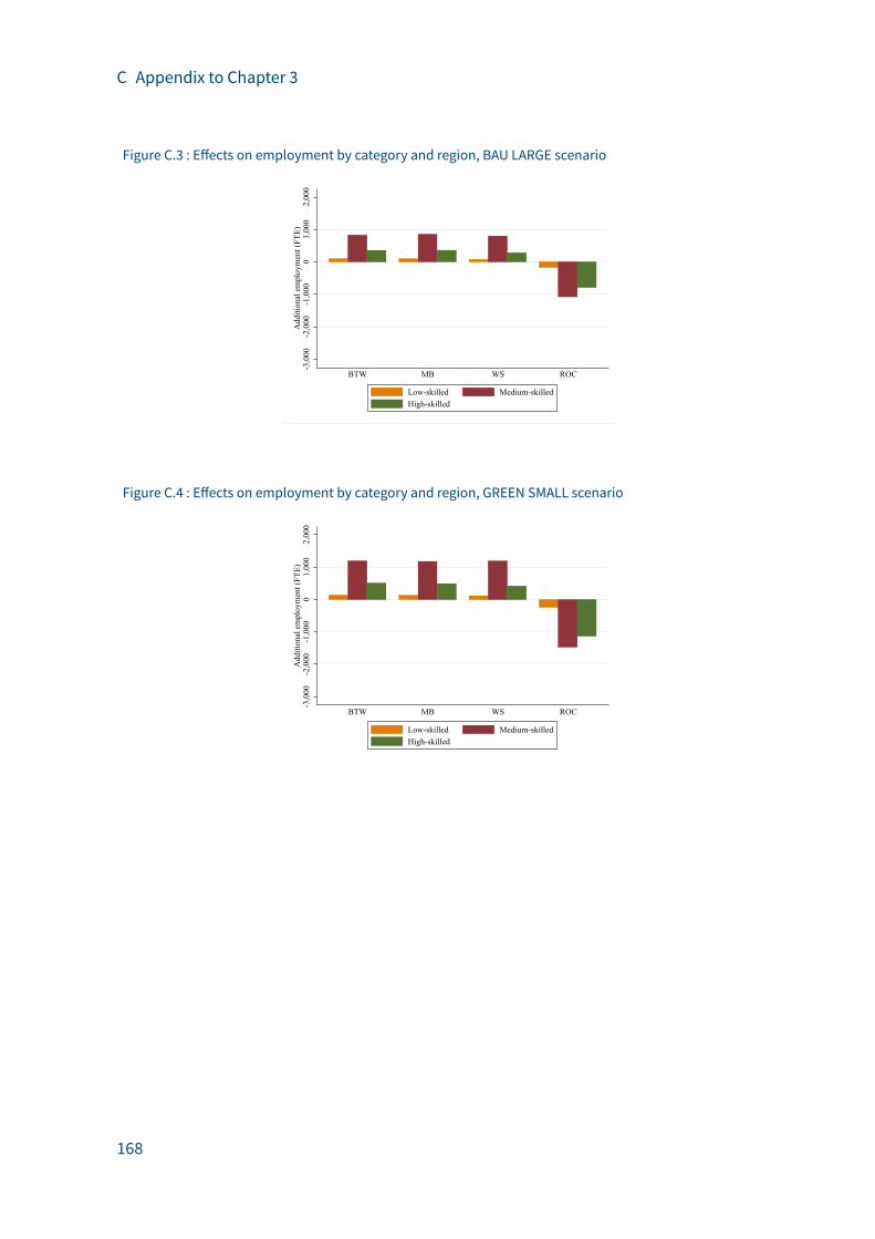
C Appendix to Chapter 3
Figure C.3 : E�ects on employment by category and region, BAU LARGE scenario
-3,0
00-2
,000
-1,0
000
1,00
02,
000
Add
ition
al e
mpl
oym
ent (
FTE)
BTW MB WS ROC
Low-skilled Medium-skilledHigh-skilled
Figure C.4 : E�ects on employment by category and region, GREEN SMALL scenario
-3,0
00-2
,000
-1,0
000
1,00
02,
000
Add
ition
al e
mpl
oym
ent (
FTE)
BTW MB WS ROC
Low-skilled Medium-skilledHigh-skilled
168
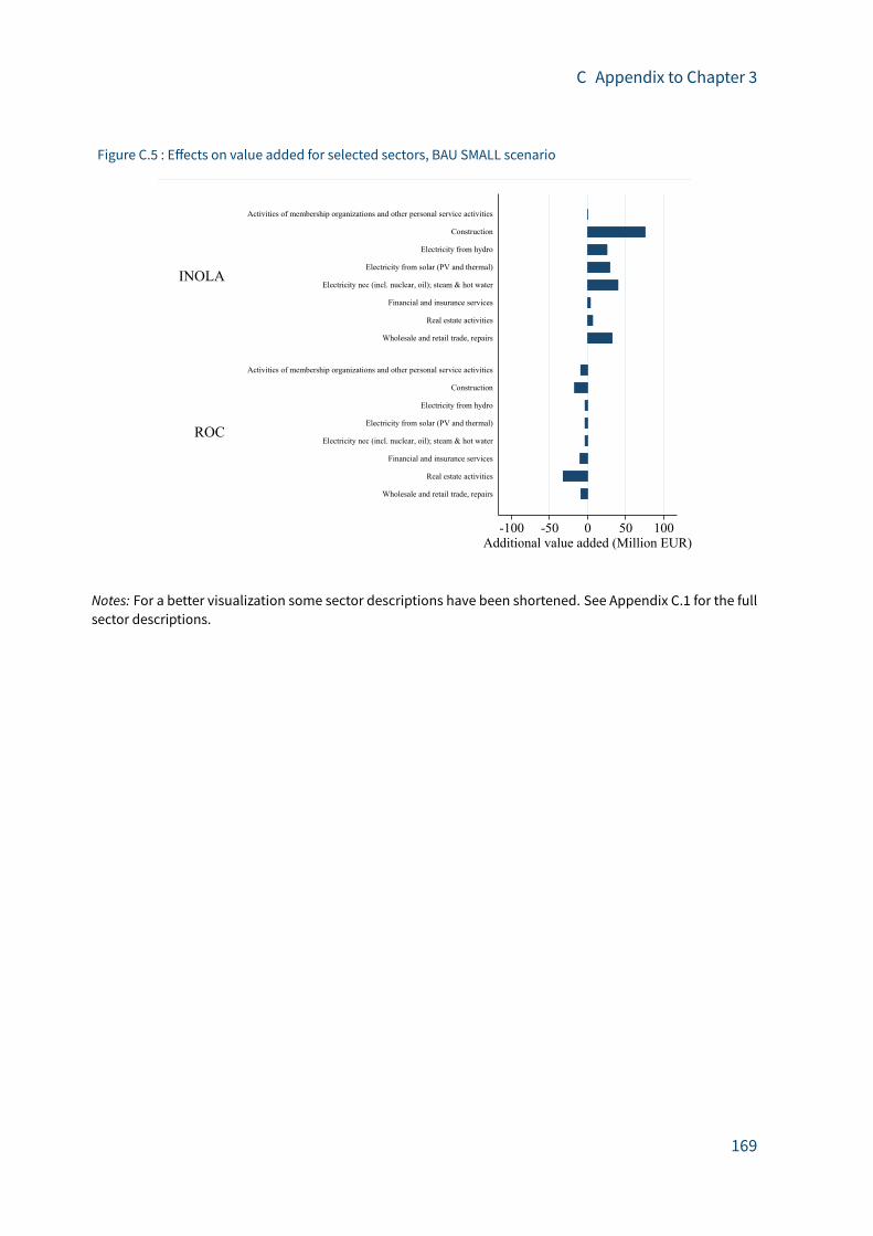
C Appendix to Chapter 3
Figure C.5 : E�ects on value added for selected sectors, BAU SMALL scenario
-100 -50 0 50 100Additional value added (Million EUR)
ROC
INOLA
Wholesale and retail trade, repairs
Real estate activities
Financial and insurance services
Electricity nec (incl. nuclear, oil); steam & hot water
Electricity from solar (PV and thermal)
Electricity from hydro
Construction
Activities of membership organizations and other personal service activities
Notes: For a better visualization some sector descriptions have been shortened. See Appendix C.1 for the fullsector descriptions.
169
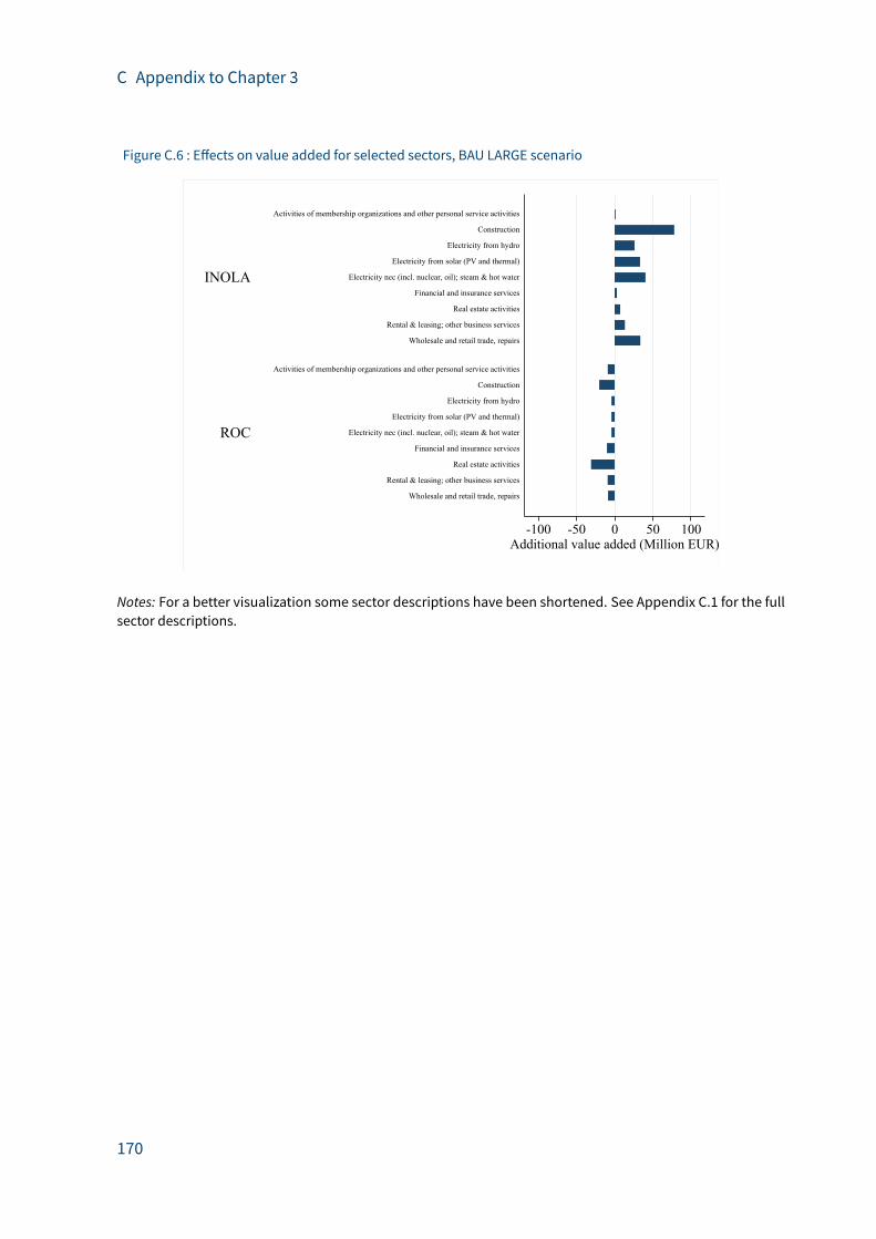
C Appendix to Chapter 3
Figure C.6 : E�ects on value added for selected sectors, BAU LARGE scenario
-100 -50 0 50 100Additional value added (Million EUR)
ROC
INOLA
Wholesale and retail trade, repairs
Rental & leasing; other business services
Real estate activities
Financial and insurance services
Electricity nec (incl. nuclear, oil); steam & hot water
Electricity from solar (PV and thermal)
Electricity from hydro
Construction
Activities of membership organizations and other personal service activities
Notes: For a better visualization some sector descriptions have been shortened. See Appendix C.1 for the fullsector descriptions.
170
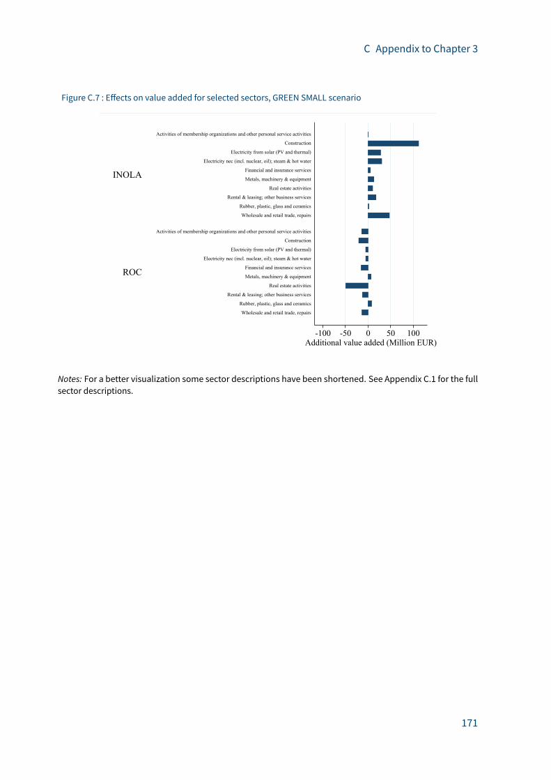
C Appendix to Chapter 3
Figure C.7 : E�ects on value added for selected sectors, GREEN SMALL scenario
-100 -50 0 50 100Additional value added (Million EUR)
ROC
INOLA
Wholesale and retail trade, repairs
Rubber, plastic, glass and ceramics
Rental & leasing; other business services
Real estate activities
Metals, machinery & equipment
Financial and insurance services
Electricity nec (incl. nuclear, oil); steam & hot water
Electricity from solar (PV and thermal)
Construction
Activities of membership organizations and other personal service activities
Notes: For a better visualization some sector descriptions have been shortened. See Appendix C.1 for the fullsector descriptions.
171
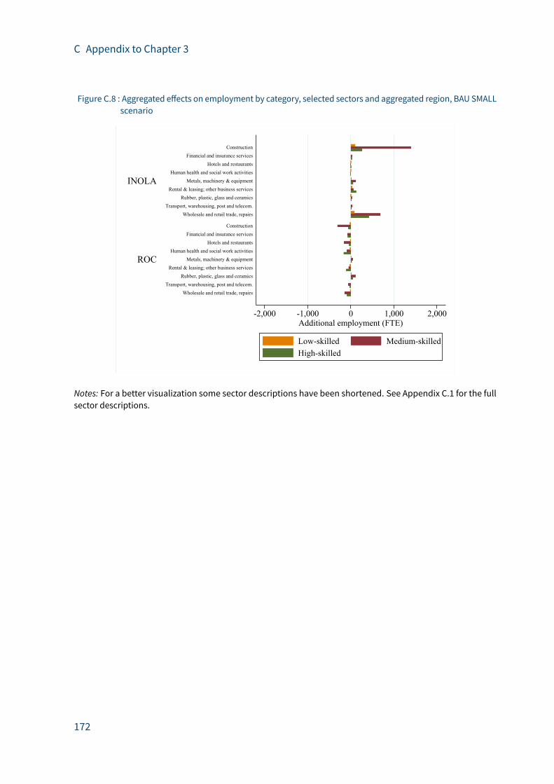
C Appendix to Chapter 3
Figure C.8 : Aggregated e�ects on employment by category, selected sectors and aggregated region, BAU SMALLscenario
-2,000 -1,000 0 1,000 2,000Additional employment (FTE)
ROC
INOLA
Wholesale and retail trade, repairsTransport, warehousing, post and telecom.
Rubber, plastic, glass and ceramicsRental & leasing; other business services
Metals, machinery & equipmentHuman health and social work activities
Hotels and restaurantsFinancial and insurance services
Construction
Wholesale and retail trade, repairsTransport, warehousing, post and telecom.
Rubber, plastic, glass and ceramicsRental & leasing; other business services
Metals, machinery & equipmentHuman health and social work activities
Hotels and restaurantsFinancial and insurance services
Construction
Low-skilled Medium-skilledHigh-skilled
Notes: For a better visualization some sector descriptions have been shortened. See Appendix C.1 for the fullsector descriptions.
172

C Appendix to Chapter 3
Figure C.9 : Aggregated e�ects on employment by category, selected sectors and aggregated region, BAU LARGEscenario
-2,000 -1,000 0 1,000 2,000Additional employment (FTE)
ROC
INOLA
Wholesale and retail trade, repairsTransport, warehousing, post and telecom.
Rubber, plastic, glass and ceramicsRental & leasing; other business services
Metals, machinery & equipmentHuman health and social work activities
Hotels and restaurantsFinancial and insurance services
Construction
Wholesale and retail trade, repairsTransport, warehousing, post and telecom.
Rubber, plastic, glass and ceramicsRental & leasing; other business services
Metals, machinery & equipmentHuman health and social work activities
Hotels and restaurantsFinancial and insurance services
Construction
Low-skilled Medium-skilledHigh-skilled
Notes: For a better visualization some sector descriptions have been shortened. See Appendix C.1 for the fullsector descriptions.
173
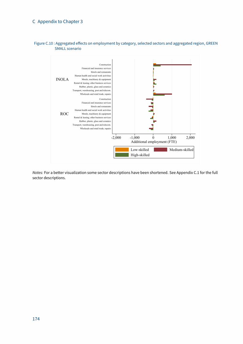
C Appendix to Chapter 3
Figure C.10 : Aggregated e�ects on employment by category, selected sectors and aggregated region, GREENSMALL scenario
-2,000 -1,000 0 1,000 2,000Additional employment (FTE)
ROC
INOLA
Wholesale and retail trade, repairsTransport, warehousing, post and telecom.
Rubber, plastic, glass and ceramicsRental & leasing; other business services
Metals, machinery & equipmentHuman health and social work activities
Hotels and restaurantsFinancial and insurance services
Construction
Wholesale and retail trade, repairsTransport, warehousing, post and telecom.
Rubber, plastic, glass and ceramicsRental & leasing; other business services
Metals, machinery & equipmentHuman health and social work activities
Hotels and restaurantsFinancial and insurance services
Construction
Low-skilled Medium-skilledHigh-skilled
Notes: For a better visualization some sector descriptions have been shortened. See Appendix C.1 for the fullsector descriptions.
174

Bibliography
Abadie, Alberto (2020). “Statistical Nonsignificance in Empirical Economics”. American Eco-
nomic Review: Insights 2 (2), pp. 193–208.
Abadie, Alberto, Alexis Diamond, and Jens Hainmueller (2010). “Synthetic Control Methods for
Comparative Case Studies: Estimating the E�ect of California’s Tobacco Control Program”.
Journal of the American Statistical Association 105 (490), pp. 493–505.
– (2015). “Comparative Politics and the Synthetic Control Method”. American Journal of
Political Science 59 (2), pp. 495–510.
Abadie, Alberto and Javier Gardeazabal (2003). “The Economic Costs of Conflict: A Case Study
of the Basque Country”. American Economic Review 93 (1), pp. 113–132.
Acemoglu, Daron, Philippe Aghion, Leonardo Bursztyn, and David Hemous (2012). “The
Environment and Directed Technical Change”. American Economic Review 102 (1), pp. 131–
66.
ACER (2015). Report on Unit Investment Cost Indicators and Corresponding Reference Values
for Electricity and Gas Infrastructure. Ljubljana: Agency for the Cooperation for Energy
Regulators.
AEE (2012). Studienvergleich: Entwicklung der Investitionskosten neuer Kra�werke. Agentur für
Erneuerbare Energien.
Agentur für Erneuerbare Energien (2019). Daten und Fakten zur Entwicklung Erneuerbarer
Energien in einzelnen Bundesländern - Föderal Erneuerbar. URL: https://www.foederal
-erneuerbar.de/landesinfo/bundesland/BY/kategorie/solar/auswahl/296-neu%
7B%5C_%7Dinstallierte%7B%5C_%7Dlei/%7B%5C#%7Dgoto%7B%5C_%7D296 (visited on
08/27/2019).
Aghion, Philippe, Nick Bloom, Richard Blundell, Rachel Gri�ith, and Peter Howitt (2005). “Com-
petition and Innovation: An Inverted-U Relationship”. The Quarterly Journal of Economics
120 (2), pp. 701–728.
Aghion, Philippe, Antoine Dechezleprêtre, David Hemous, Ralf Martin, and John Van Reenen
(2016). “Carbon Taxes, Path Dependency, and Directed Technical Change: Evidence from
the Auto Industry”. Journal of Political Economy 124 (1), pp. 1–51.
Aghion, Philippe, John Van Reenen, and Luigi Zingales (2013). “Innovation and Institutional
Ownership”. American Economic Review 103 (1), pp. 277–304.
175
Bibliography
Allan, G., P. G. McGregor, J. K. Swales, and K. Turner (2007). “Impact of alternative electricity
generation technologies on the Scottish economy: An illustrative input-output analysis”.
Proceedings of the Institution of Mechanical Engineers, Part A: Journal of Power and Energy
221 (2), pp. 243–254.
Allen, Myles R., David J. Frame, Chris Huntingford, Chris D. Jones, Jason A. Lowe, Malte
Meinshausen, and Nicolai Meinshausen (2009). “Warming Caused by Cumulative Carbon
Emissions towards the Trillionth Tonne”. Nature 458 (7242), pp. 1163–1166.
Appel, Ian R., Todd A. Gormley, and Donald B. Keim (2016). “Passive Investors, Not Passive
Owners”. Journal of Financial Economics 121 (1), pp. 111–141.
– (2018). “Standing on the Shoulders of Giants: The E�ect of Passive Investors on Activism”.
SSRN Electronic Journal.
Atanassov, Julian (2013). “Do Hostile Takeovers Stifle Innovation? Evidence from Antitakeover
Legislation and Corporate Patenting: Takeovers and Innovation”. The Journal of Finance
68 (3), pp. 1097–1131.
Azar, José, Miguel Duro, Igor Kadach, and Gaizka Ormazabal (2020). “The Big Three and
Corporate Carbon Emissions Around the World”. SSRN Electronic Journal.
Banque de France (2015). Assessment of Risks to the French Financial System. Paris: Banque de
France.
Baron, Richard and David Fischer (2015). Divestment and Stranded Assets in the Low-Carbon
Transition. Backgroundpaper for the 32ndRoundTable on Sustainable Development. OECD.
Barradale, Merrill Jones (2014). “Investment under Uncertain Climate Policy: A Practitioners’
Perspective on Carbon Risk”. Energy Policy 69, pp. 520–535.
Batten, Sandra, Rhiannon Sowerbutts, and Misa Tanaka (2016). “Let’s Talk about the Weather:
The Impact of Climate Change on Central Banks”. Bank of England Sta� Working Paper 603.
Battiston, Stefano, Antoine Mandel, and Irene Monasterolo (2019). “CLIMAFIN Handbook:
Pricing Forward-Looking Climate Risks under Uncertainty Part 1”. SSRN Electronic Journal.
Battiston, Stefano, Antoine Mandel, Irene Monasterolo, Franziska Schütze, and Gabriele
Visentin (2017). “A Climate Stress-Test of the Financial System”. Nature Climate Change
7 (4), pp. 283–288.
Bebchuk, Lucian A., Alma Cohen, and Scott Hirst (2017). “The Agency Problems of Institutional
Investors”. Journal of Economic Perspectives 31 (3), pp. 89–112.
Benz, Sebastian, Mario Larch, and Markus Zimmer (2014). “The structure of Europe: Interna-
tional input-output analysis with trade in intermediate inputs and capital flows”. Review of
Development Economics 18 (3), pp. 461–474.
176

Bibliography
Berg, Florian, Julian Koelbel, and Roberto Rigobon (2019). “Aggregate Confusion: The Diver-
gence of ESG Ratings”. MIT Sloan School Working Paper 5822-19.
Bernstein, Shai (2015). “Does Going Public A�ect Innovation?” The Journal of Finance 70 (4),
pp. 1365–1403.
Berridge, Rob and Natasha Nurjadin (2020). Why Do Some Large Asset Managers Still Vote
against Most Climate-Related Shareholder Proposals? URL: https://www.ceres.org/ne
ws-center/blog/why-do-some-large-asset-managers-still-vote-against-mos
t-climate-related.
Bessembinder, Hendrik and Michael L. Lemmon (2002). “Equilibrium Pricing and Optimal
Hedging in Electricity Forward Markets”. The Journal of Finance 57 (3), pp. 1347–1382.
Beyer, Mila, Dirk Czarnitzki, and Kornelius Kra� (2012). “Managerial Ownership, Entrenchment
and Innovation”. Economics of Innovation and New Technology 21 (7), pp. 679–699.
Bhattacharya, Utpal, Po-Hsuan Hsu, Xuan Tian, and Yan Xu (2017). “What A�ects Innovation
More: Policy or Policy Uncertainty?” Journal of Financial and Quantitative Analysis 52 (5),
pp. 1869–1901.
Bickel, Peter, Tobias Kelm, and Dietmar Edler (2012). Evaluierung Der Inländischen KfW-
Programme Zur Förderung Erneuerbarer Energien Im Jahr 2010. Gutachten im Au�rag der
KfW Bankengruppe. Stuttgart: Zentrum für Sonnenenergie- und Wassersto�-Forschung.
Bickel, Peter, Andreas Püttner, and Tobias Kelm (2009). Verbesserte Abschätzung des in Baden-
Württemberg wirksamen Investitionsimpulses durch die Förderung Erneuerbarer Energien.
Stuttgart.
Binder, John J. (1985a). “Measuring the E�ects of Regulation with Stock Price Data”. The RAND
Journal of Economics, pp. 167–183.
– (1985b). “On the Use of the Multivariate Regression Model in Event Studies”. Journal of
Accounting Research, pp. 370–383.
Blesl, Markus, Ste�en Wissel, and Ulrich Fahl (2012). “Stromerzeugung 2030—Mit welchen
Kosten ist zu rechnen?” Energiewirtscha�liche Tagesfragen 62 (10), p. 20.
Blundell, Richard, Rachel Gri�ith, and John Van Reenen (1999). “Market Share, Market Value
and Innovation in a Panel of BritishManufacturing Firms”. Review of Economic Studies 66 (3),
pp. 529–554.
Blundell, Richard, Rachel Gri�ith, and Frank Windmeijer (2002). “Individual E�ects and Dy-
namics in Count Data Models”. Journal of Econometrics, pp. 113–131.
Böhmer, Michael, Helmut Kirchner, Jens Hobohm, Johann Weiß, and Alexander Piegsa (2015).
Wertschöpfungs- und Beschä�igungse�ekte der Energiewirtscha�. Munich, Basel, Berlin.
177

Bibliography
Borochin, Paul, Jie Yang, and Rongrong Zhang (2020). “Common Ownership Types and Their
E�ects on Innovation and Competition”. SSRN Electronic Journal.
Breitschopf, Barbara, Marian Klobasa, Jan Steinbach, Frank Sensfuss, Jochen Diekmann,
Ulrike Lehr, and Juri Horst (2015). Monitoring der Kosten- und Nutzenwirkungen des Ausbaus
erneuerbarer Energien im Jahr 2014. URL: http://www.erneuerbare-energien.de/file
admin/ee-import/files/pdfs/allgemein/application/pdf/knee%7B%5C_%7Dupda
te%7B%5C_%7D2012%7B%5C_%7Dbf.pdf.
Bretschger, Lucas and Andreas Schaefer (2017). “Dirty History versus Clean Expectations: Can
Energy Policies Provide Momentum for Growth?” European Economic Review 99, pp. 170–
190.
Breyer, Christian, Berit Müller, Caroline Möller, Elisa Gaudchau, Ludwig Schneider, Kevin
Gajkowski, Matthias Resch, and Guido Pleßmann (2013). Vergleich und Optimierung von
zentral und dezentral orientierten Ausbaupfaden zu einer Stromversorgung aus Erneuer-
baren Energien in Deutschland. Studie des Reiner Lemoine Instituts gGmbH im Au�rag
von Heleakala Sti�ung, 100 prozent erneuerbar sti�ung und BVMW Bundesverbandmittel-
ständische Wirtscha�. Berlin.
Brown, Jason P., John Pender, Ryan Wiser, Eric Lantz, and Ben Hoen (2012). “Ex post analysis
of economic impacts fromwind power development in U.S. counties”. Energy Economics
34 (6), pp. 1743–1754.
Buchheim, Lukas, Martin Watzinger, and Matthias Wilhelm (2020). “Job creation in tight and
slack labor markets”. Journal of Monetary Economics 114, pp. 126–143.
Bundesministerium für Wirtscha� und Energie (2015). Der Nationale Klimaschutzbeitrag der
deutschen Stromerzeugung. Ergebnisse der Task Force "CO2-Minderung". Berechnungen:
Öko-Institut e.V. & Prognos AG.
Bushee, Brian J. (1998). “The Influence of Institutional Investors on Myopic R&D Investment
Behavior”. The Accounting Review, pp. 305–333.
Byrd, John W. and Elizabeth S. Cooperman (2016). Investors and Stranded Asset Risk: Evi-
dence from Shareholder Responses to Carbon Capture and Sequestration (CCS) Events. SSRN
Scholarly Paper. Rochester, NY: Social Science Research Network.
Caldecott, Ben (2017). “Introduction to Special Issue: Stranded Assets and the Environment”.
Journal of Sustainable Finance & Investment 7 (1), pp. 1–13.
Caldecott, Ben, Geraldine Bouveret, Gerard Dericks, Lucas Kruitwagen, Daniel J. Tulloch, and
Xiawei Liao (2017). “Managing the political economy frictions of closing coal in China”.
178
Bibliography
Sustainable Finance Programme – Discussion Paper, Smith School of Enterprise and the
Environment, Oxford University.
Caldecott, Ben, Elizabeth Harnett, Theodor Cojoianu, Irem Kok, and Alexander Pfei�er (2016).
Stranded Assets: A Climate Risk Challenge. Washington, D.C.: Inter-American Development
Bank (IDB).
Calel, Raphael and Antoine Dechezleprêtre (2016). “Environmental Policy and Directed Tech-
nological Change: Evidence from the European Carbon Market”. Review of Economics and
Statistics 98 (1), pp. 173–191.
Campbell, John Y., AndrewW. Lo, A. CraigMacKinlay, et al. (1997). The econometrics of financial
markets. Vol. 2. Princeton, NJ: Princeton University Press.
Carattini, Stefano and Suphi Sen (2019). “Carbon Taxes and Stranded Assets: Evidence from
Washington State”. CESifo Working Paper 7785.
Chemmanur, Thomas J., Elena Loutskina, and Xuan Tian (2014). “Corporate Venture Capital,
Value Creation, and Innovation”. Review of Financial Studies 27 (8), pp. 2434–2473.
Christensen, Clayton M, Michael Raynor, and Rory McDonald (2015). “What Is Disruptive
Innovation?” Harvard Business Review 93 (12), pp. 44–53.
Cludius, Johanna, Hauke Hermann, Felix Chr. Matthes, and Verena Graichen (2014). “The
merit order e�ect of wind and photovoltaic electricity generation in Germany 2008–2016:
Estimation and distributional implications”. Energy Economics 44, pp. 302–313.
Cockburn, Iain and Zvi Griliches (1988). “Industry E�ects and Appropriability Measures in
the Stock Market’s Valuation of R&D and Patents”. American Economic Review: Papers and
Proceedings 78 (2), pp. 419–423.
Collier, P. and A. J. Venables (2014). “Closing Coal: Economic and Moral Incentives”. Oxford
Review of Economic Policy 30 (3), pp. 492–512.
Crane, Alan D., Sébastien Michenaud, and James P. Weston (2016). “The E�ect of Institutional
Ownership on Payout Policy: Evidence from Index Thresholds”. Review of Financial Studies
29 (6), pp. 1377–1408.
Crost, Benjamin and Christian P. Traeger (2014). “Optimal CO2 Mitigation under Damage Risk
Valuation”. Nature Climate Change 4 (7), pp. 631–636.
Danner, Martin, EvaHalwachs, Veronika Locherer, AnaMariaMontoyaGómez, Andrea Reimuth,
and Markus Zimmer (2019). INOLA-Arbeitsbericht Nr. 10. Simulation regionaler Energiep-
fade im Oberland bis 2034/2045: Akteursentscheidungen, Energie- und Sto�ströme sowie
ökonomische E�ekte. URL: https://inola-region.de/download/a4gs9u1mm0veeq58n
7u0578ni7f/INOLA_Arbeitsbericht_Nr10.pdf.
179
Bibliography
Dasgupta, Partha and Joseph Stiglitz (1980). “Industrial Structure and theNature of Innovative
Activity”. The Economic Journal 90 (358), p. 266.
Davis, Lucas W. and Lutz Kilian (2011). “Estimating the E�ect of a Gasoline Tax on Carbon
Emissions”. Journal of Applied Econometrics 26 (7), pp. 1187–1214.
Davis, Steven J. and Robert H Socolow (2014). “Commitment Accounting of CO2 Emissions”.
Environmental Research Letters 9 (8), p. 084018.
Dechezleprêtre, Antoine, Ralf Martin, and Myra Mohnen (2017). “Knowledge Spillovers from
Clean and Dirty Technologies”. Grantham Research Institute on Climate Change and the
Environment Working Paper 135.
Delis, Manthos D, Kathrin de Grei�, and Steven Ongena (2019). “Being Stranded with Fossil
Fuel Reserves? Climate Policy Risk and the Pricing of Bank Loans”. Swiss Finance Institute
Research Paper Series 18 (10).
Deutsche Energie-Agentur (2012). Ausbau- und Innovationsbedarf der Stromverteilnetze in
Deutschland bis 2030. Berlin.
Di Maria, Corrado, Ian Lange, and Edwin van der Werf (2014). “Should We BeWorried about
the Green Paradox? Announcement E�ects of the Acid Rain Program”. European Economic
Review 69, pp. 143–162.
Di Maria, Corrado and Sjak Smulders (2017). “A Paler Shade of Green: Environmental Policy
under Induced Technical Change”. European Economic Review 99, pp. 151–169.
Dietz, Simon, Alex Bowen, Charlie Dixon, and Philip Gradwell (2016). “‘Climate Value at Risk’
of Global Financial Assets”. Nature Climate Change 6 (7), pp. 676–679.
Dimson, Elroy, Oğuzhan Karakaş, and Xi Li (2015). “Active Ownership”. Review of Financial
Studies 28 (12), pp. 3225–3268.
Dumont, Ulrich and Rita Keuneke (2011). Vorbereitung und Begleitung der Erstellung des
Erfahrungsberichtes 2011 Gemäß § 65 EEG - Endbericht des Vorhabens IId Wasserkra�. Im
Au�rag des Bundesministeriums für Umwelt, Naturschutz und Reaktorsicherheit. Aachen:
Ingenieurbüro Floecksmühle.
Dyck, Alexander, Karl V. Lins, Lukas Roth, and Hannes F. Wagner (2019). “Do Institutional In-
vestors Drive Corporate Social Responsibility? International Evidence”. Journal of Financial
Economics 131 (3), pp. 693–714.
ENTSO-E (2017a). Information upon the Lengths of Circuits on December 31st. URL: https:
//www.entsoe.eu/db-query/miscellaneous/lengths-of-circuits (visited on
01/31/2017).
180
Bibliography
– (2017b). Installed Capacity per Production Type. URL: https://transparency.entsoe.
eu/generation/r2/installedGenerationCapacityAggregation/show (visited on
01/31/2017).
Erickson, Peter, Sivan Kartha, Michael Lazarus, and Kevin Tempest (2015). “Assessing Carbon
Lock-In”. Environmental Research Letters 10 (8), p. 084023.
Eurogas (2008). Statistics 2008.
European Systemic Risk Board (2016a). “Too Late, Too Sudden: Transition to a Low-Carbon
Economy and Systemic Risk”. Reports of the Advisory Scientific Committee 6.
– (2016b). “Too Late, Too Sudden: Transition to a Low-Carbon Economy and Systemic Risk”.
Reports of the Advisory Scientific Committee 6.
Eurostat (2016a). Cross-Classification of Fixed Assets by Industry and by Asset (Stocks). URL:
http://appsso.eurostat.ec.europa.eu/nui/show.do?dataset=nama_10_nfa_s
t&lang=en.
– (2016b). Supply, Transformation and Consumption of Heat - Annual Data. URL: http://
ec.europa.eu/eurostat/en/web/products-datasets/-/NRG_106A (visited on
01/20/2017).
Faehn, Taran, Cathrine Hagem, Lars Lindholt, Stale Maeland, and Knut Einar Rosendahl (2014).
“Climate Policies in a Fossil Fuel Producing Country - Demand Versus Supply Side Policies”.
SSRN Scholarly Paper.
Fama, EugeneF., LawrenceFisher,MichaelC. Jensen, andRichardRoll (1969). “TheAdjustment
of Stock Prices to New Information”. International Economic Review 10 (1), pp. 1–21.
Feenstra, Robert C. (2004). Advanced International Trade: Theory and Evidence. Princeton, NJ:
Princeton Univ. Press.
Fichtner, Jan, Eelke M. Heemskerk, and Javier Garcia-Bernardo (2017). “Hidden Power of
the Big Three? Passive Index Funds, Re-Concentration of Corporate Ownership, and New
Financial Risk”. Business and Politics 19 (2), pp. 298–326.
Fisher, Eric O.N. and Kathryn G. Marshall (2011). “The structure of the American economy”.
Review of International Economics 19 (1), pp. 15–31.
Fried, Stephie (2018). “ClimatePolicyand Innovation: AQuantitativeMacroeconomicAnalysis”.
American Economic Journal: Macroeconomics 10 (1), pp. 90–118.
Fried, Stephie, Kevin Novan, andWilliam B Peterman (2020). “The Macro E�ects of Climate
Policy Uncertainty”. Working Paper.
Gibson, Rajna and Philipp Krueger (2017). “The Sustainability Footprint of Institutional In-
vestors”. ECGI Working Paper (571).
181
Bibliography
Gillingham, Kenneth and James H Stock (2018). “The Cost of Reducing Greenhouse Gas
Emissions”. Journal of Economic Perspectives 32 (4), pp. 53–72.
Gri�in, Paul A., Amy Myers Ja�e, David H. Lont, and Rosa Dominguez-Faus (2015). “Science
and the Stock Market: Investors’ Recognition of Unburnable Carbon”. Energy Economics 52,
pp. 1–12.
Grözinger, Jan, Thomas Boermans, and Michelle Bosquet (2013). Heat Roadmap Europe 2050.
Second Pre-Study for the EU27. For Euroheat & Power. Aalborg: Department of Development
and Planning, Aalborg University.
Guidolin, Massimo and Eliana La Ferrara (2007). “Diamonds Are Forever, Wars Are Not: Is
Conflict Bad for Private Firms?” American Economic Review 97 (5), pp. 1978–1993.
Hall, Bronwyn H., Adam Ja�e, and Manuel Trajtenberg (2005). “Market Value and Patent
Citations”. RAND Journal of economics, pp. 16–38.
Hall, BronwynH. andJoshLerner (2010). “TheFinancingofR&Dand Innovation”. In: Handbook
of the Economics of Innovation. Vol. 1. Elsevier, pp. 609–639.
Harstad, Bård (2012). “Buy Coal! A Case for Supply-Side Environmental Policy”. Journal of
Political Economy 120 (1), pp. 77–115.
Hassan, Tarek A., Stephan Hollander, Laurence van Lent, and Ahmed Tahoun (2019). “Firm-
Level Political Risk: Measurement and E�ects”. The Quarterly Journal of Economics 134 (4),
pp. 2135–2202.
– (2020a). “Firm-Level Exposure to Epidemic Diseases: Covid-19, SARS, and H1N1”. NBER
Working Paper 26971.
– (2020b). “The Global Impact of Brexit Uncertainty”. NBERWorking Paper 26609.
Hausman, Jerry, Bronwyn H. Hall, and Zvi Griliches (1984). “Econometric Models for Count
Data with an Application to the Patents-R & D Relationship”. Econometrica 52 (4), pp. 909–
938.
He, Jie (Jack) and Jiekun Huang (2017). “Product Market Competition in a World of Cross-
Ownership: Evidence from Institutional Blockholdings”. The Review of Financial Studies
30 (8), pp. 2674–2718.
Healy, Noel and John Barry (2017). “Politicizing energy justice and energy system transitions:
Fossil fuel divestment and a “just transition””. Energy Policy 108, pp. 451–459.
Heindl, Peter and Sebastian Voigt (2012). “Employment E�ects of Regional Climate Policy:
The Case of Renewable Energy Promotion by Feed-In Tari�s”. ZEW Discussion Paper 12-066.
Hinz, Eberhard (2015). Kosten energierelevanter Bau- und Anlagenteile bei der energetischen
Modernisierung von Altbauten. Darmstadt: Institut Wohnen und Umwelt GmbH.
182

Bibliography
Hirschl, Bernd, Astrid Aretz, Andreas Prahl, Timo Böther, Katharina Heinbach, Daniel Pick, and
Simon Funcke (2010). Kommunale Wertschöpfung durch Erneuerbare Energien. Schri�en-
reihe des IÖW 196. Berlin: Institut für ökologische Wirtscha�sforschung.
Hirschl, Bernd, Katharina Heinbach, Andreas Prahl, Steven Salecki, Astrid Aretz, and Julika
Weiß (2015). Wertschöpfung durch Erneuerbare Energien. Ermittlung der E�ekte auf Länder-
und Bundesebene. Schri�enreihe des IÖW 210. Berlin: Institut für ökologische Wirtscha�s-
forschung.
Hobohm, Jens and Stefan Mellahn (2010). Investitionen Durch Den Ausbau Erneuerbarer Ener-
gien in Deutschland. Im Au�rag des Bundesverbandes Erneuerbare Energie e.V., der Agentur
für Erneuerbare Energien und der HANNOVER MESSE. Berlin: prognos AG.
Höher, Martin, Andrea Jamek, Sophie Limbeck, Oskar Mair am Tinkhof, Johannes Schmidl,
and Günter Rudolf Simander (2015). Regionale Wertschöpfung und Beschä�igung durch
Energie aus fester Biomasse. Studie im Au�rag des Klima- und Energiefonds. Wien: Austrian
Energy Agency.
Hollander, Stephan, Maarten Pronk, and Erik Roelofsen (2010). “Does Silence Speak? An
Empirical Analysis of Disclosure Choices During Conference Calls”. Journal of Accounting
Research 48 (3), pp. 531–563.
HSBC (2012). Coal and Carbon. Stranded Assets: Assessing the Risk. URL: https://www.re
search.hsbc.com/midas/Res/RDV?p=pdf&key=dXwE9bC8qs&n=333473.PDF (visited on
02/24/2017).
Hsu, Po-Hsuan and Hao Liang (2017). “Leviathan Inc. and Corporate Environmental Engage-
ment”. ECGI Working Paper (526).
ICF Consulting (2003). Overview of the Potential for Undergrounding the Electricity Networks in
Europe. Prepared for the DG TREN/European Commission. London.
IEA (2007). Climate Policy Uncertainty and Investment Risk. Paris: OECD Publishing.
– (2013). Redrawing the Energy-Climate Map - World Energy Outlook Special Report. Paris:
OECD/IEA Publishing.
– (2015). Projected Costs of Generating Electricity 2015. Tech. rep. International Energy Agency
and Nuclear Energy Agency.
– (2017). OECD - Electricity andheat generation, IEA Electricity InformationStatistics (database).
URL: https://doi.org/10.1787/data-00457-en (visited on 09/28/2017).
IPCC (2014a). ClimateChange2014Mitigationof ClimateChange: WorkingGroup III Contribution
to the Fi�h Assessment Report of the Intergovernmental Panel on Climate Change. Ed. by
O. Edenhofer, R. Pichs-Madruga, Y. Sokona, E. Farahani, S. Kadner, K. Seyboth, A. Adler,
183
Bibliography
I. Baum, S. Brunner, P. Eickemeier, B. Kriemann, J. Savolainen, S. Schlömer, C. von Stechow,
T. Zwickel, and J.C. Minx. Cambridge, UK and New York, NY, USA: Cambridge University
Press.
IPCC (2014b). Climate Change 2014: Impacts, Adaptation, and Vulnerability. Part A: Global
and Sectoral Aspects. Contribution of Working Group II to the Fi�h Assessment Report of the
Intergovernmental Panel on Climate Change. Ed. by C.B. Field, V.R. Barros, D.J. Dokken,
K.J. Mach, M.D. Mastrandrea, T.E. Bilir, M. Chatterjee, K.L. Ebi, Y.O. Estrada, R.C. Genova,
B. Girma, E.S. Kissel, A.N. Levy, S. MacCracken, P.R. Mastrandrea, and L.L. White. Cambridge,
UK and New York, NY, USA: Cambridge University Press.
IRENA (2016a). Data and Statistics - IRENA REsource. URL: http://resourceirena.irena.
org/gateway/dashboard/?topic=4&subTopic=54 (visited on 01/31/2017).
– (2016b). Renewable Energy Benefits: Measuring the Economics. Abu Dhabi: International
Renewable Energy Agency (IRENA).
– (2017a). “Global Energy Transition Prospects and the Role of Renewables”. In: Perspectives
for the Energy Transition: Investment Needs for a Low-Carbon Energy System. Abu Dhabi:
International Renewable Energy Agency (IRENA).
– (2017b). Stranded Assets and Renewables: How the Energy Transition A�ects the Value of
Energy Reserves, Buildings and Capital Stock. Abu Dhabi: International Renewable Energy
Agency (IRENA).
IWU (2018). Informationen EnEV-XL. URL: https://www.iwu.de/veroeffentlichung
en/fachinformationen/energiebilanzen/informationen-enev-xl/ (visited on
09/26/2018).
Iyer, Gokul C., James A. Edmonds, Allen A. Fawcett, Nathan E. Hultman, Jameel Alsalam,
Ghassem R. Asrar, Katherine V. Calvin, Leon E. Clarke, Jared Creason, Minji Jeong, et al.
(2015). “The contribution of Paris to limit global warming to 2°C”. Environmental Research
Letters 10 (12).
Jackson, Randall (2014). “Cross-Hauling in Input-Output Tables : Comments on CHARM”.
Regional Research Institute Working Paper Series 2014-2.
Jenkins, Jesse D. (2014). “Political Economy Constraints on Carbon Pricing Policies: What
Are the Implications for Economic E�iciency, Environmental E�icacy, and Climate Policy
Design?” Energy Policy 69, pp. 467–477.
Jiang, Xuanyu and Qingbo Yuan (2018). “Institutional Investors’ Corporate Site Visits and
Corporate Innovation”. Journal of Corporate Finance 48, pp. 148–168.
184

Bibliography
Johnson, Nils, Volker Krey, David L McCollum, Shilpa Rao, Keywan Riahi, and Joeri Rogelj
(2015). “Stranded on a low-carbon planet: Implications of climate policy for the phase-out
of coal-based power plants”. Technological Forecasting and Social Change 90, pp. 89–102.
Keller, Andreas (2010). “Competition E�ects of Mergers: An Event Study of the German Elec-
tricity Market”. Energy Policy 38 (9), pp. 5264–5271.
Kerr, William R and Ramana Nanda (2015). “Financing Innovation”. Annual Review of Financial
Economics 7, pp. 445–462.
Kiso, Takahiko (2019). “Environmental Policy and Induced Technological Change: Evidence
fromAutomobile Fuel EconomyRegulations”. Environmental and Resource Economics 74 (2),
pp. 785–810.
Koch, Nicolas, Godefroy Grosjean, Sabine Fuss, and Ottmar Edenhofer (2016). “Politics Mat-
ters: Regulatory Events as Catalysts for Price Formation under Cap-and-Trade”. Journal of
Environmental Economics and Management 78, pp. 121–139.
Kogan, Leonid, Dimitris Papanikolaou, Amit Seru, and Noah Sto�man (2017). “Technological
Innovation, Resource Allocation, and Growth”. The Quarterly Journal of Economics 132 (2),
pp. 665–712.
Kost, Christoph, Johannes N. Mayer, Jessica Thomsen, Charlotte Senkpiel, Simon Philipps, Se-
bastianNold, Simon Lude, and Thomas Schlegl (2013). Stromgestehungskosten Erneuerbare
Energien. Freiburg: Fraunhofer Institut für Solare Energiesysteme ISE.
Kronenberg, Tobias (2009). “Construction of Regional Input-Output Tables Using Nonsurvey
Methods”. International Regional Science Review 32 (1), pp. 40–64.
Krueger, Philipp, Zacharias Sautner, and Laura T. Starks (2020). “The Importance of Climate
Risks for Institutional Investors”. The Review of Financial Studies 33 (3), pp. 1067–1111.
Krugman, Paul (1991). “History Versus Expectations”. The Quarterly Journal of Economics
106 (2), p. 651.
Kruse, Tobias, Myra Mohnen, Peter Pope, and Misato Sato (2020). “Green Revenues, Profitabil-
ity and Market Valuation: Evidence from a Global Firm Level Dataset”. Grantham Research
Institute on Climate Change and the Environment Working Paper 331.
Kruse, Tobias, Myra Mohnen, and Misato Sato (2020). “Are Financial Markets Aligned with
Climate Action? New Evidence from the Paris Agreement”. Grantham Research Institute on
Climate Change and the Environment Working Paper 364.
Lambertini, Luca, Joanna Poyago-Theotoky, and Alessandro Tampieri (2017). “Cournot
Competition and “Green” Innovation: An Inverted-U Relationship”. Energy Economics 68,
pp. 116–123.
185
Bibliography
Lamdin, Douglas J. (2001). “Implementing and Interpreting Event Studies of Regulatory
Changes”. Journal of Economics and Business, p. 13.
Lanzi, Elisa, Elena Verdolini, and Ivan Haščič (2011). “E�iciency-Improving Fossil Fuel Tech-
nologies for Electricity Generation: Data Selection and Trends”. Energy Policy 39 (11),
pp. 7000–7014.
Leggett, Jeremy K. (2014). The Energy of Nations: Risk Blindness and the Road to Renaissance.
1. ed. London: Routledge.
Lehr, Ulrike, Dietmar Edler, Marlene O’Sullivan, Frank Peter, and Peter Bickel (2015). Beschä�i-
gung durch erneuerbare Energien in Deutschland: Ausbau und Betrieb, heute undmorgen.
Osnabrück, Berlin, Stuttgart: Studie im Au�rag des Bundesministeriums für Wirtscha� und
Energie.
Lehr, Ulrike, Christian Lutz, Dietmar Edler, Marlene O’Sullivan, Kristina Nienhaus, Joachim
Nitsch, BarbaraBreitschopf, Peter Bickel, andMarionOttmüller (2011). Kurz- und langfristige
Auswirkungen des Ausbaus der erneuerbaren Energien auf den deutschen Arbeitsmarkt. Os-
nabrück, Berlin, Karlsruhe, Stuttgart: Studie imAu�ragdesBundesministeriums fürUmwelt,
Naturschutz und Reaktorsicherheit., p. 239.
Lehr, Ulrike, Joachim Nitsch, Marlene Kratzat, Christian Lutz, and Dietmar Edler (2008). “Re-
newable energy and employment in Germany”. Energy Policy 36 (1), pp. 108–117.
Lemoine, Derek (2017). “Green Expectations: Current E�ects of Anticipated Carbon Pricing”.
Review of Economics and Statistics 99 (3).
Lerner, Josh, Morten Sorensen, and Per Strömberg (2011). “Private Equity and Long-Run
Investment: The Case of Innovation”. The Journal of Finance 66 (2), pp. 445–477.
Li, Shanjun, Joshua Linn, and Erich Muehlegger (2014). “Gasoline Taxes and Consumer Behav-
ior”. American Economic Journal: Economic Policy 6 (4), pp. 302–342.
Linn, Joshua (2010). “The E�ect of Cap-and-Trade Programs on Firms’ Profits: Evidence from
the Nitrogen Oxides Budget Trading Program”. Journal of Environmental Economics and
Management 59 (1), pp. 1–14.
Loga, Tobias, Britta Stein, Nikolaus Diefenbach, and Rolf Born (2015). Deutsche Wohnge-
bäudetypologie: Beispielha�e Maßnahmen zur Verbesserung der Energiee�izienz. 2nd ed.
Darmstadt: Institut Wohnen und Umwelt GmbH.
López, Ángel L. and Xavier Vives (2019). “OverlappingOwnership, R&DSpillovers, and Antitrust
Policy”. Journal of Political Economy 127 (5), pp. 2394–2437.
186

Bibliography
Lutz, Christian, Dietmar Lindenberger, and Andreas Kemmler (2014). Endbericht Gesamt-
wirtscha�liche E�ekte der Energiewende. Osnabrück, Köln, Basel: Projekt Nr. 31/13 des
Bundesministeriums für Wirtscha� und Energie.
MacKinlay, A. Craig (1997). “Event Studies in Economics and Finance”. Journal of Economic
Literature 35 (1), pp. 13–39.
Manley, David, James Cust, and Giorgia Cecchinato (2016). “Stranded Nations? The Climate
Policy Implications for Fossil Fuel-Rich Developing Countries”. OxCarre Policy Paper series
34.
McGlade, Christophe and Paul Ekins (2015). “The Geographical Distribution of Fossil Fuels
Unused When Limiting Global Warming to 2◦C”. Nature 517 (7533), pp. 187–190.
Meinshausen, Malte, Nicolai Meinshausen, William Hare, Sarah C. B. Raper, Katja Frieler, Reto
Knutti, David J. Frame, and Myles R. Allen (2009). “Greenhouse-Gas Emission Targets for
Limiting Global Warming to 2◦C”. Nature 458 (7242), pp. 1158–1162.
Meyer, Ina andMarkWolfgangSommer (2014). Employment E�ects of Renewable Energy Supply
A Meta Analysis. WWWforEurope Policy Paper series 12. Prepared by Austrian Institute of
Economic Research (WIFO).
Mier, Mathias and Christoph Weissbart (2019). “Power Markets in Transition: Decarbonization,
Energy E�iciency, and Short-Term Demand Response”. Ifo Working Paper 284.
Monasterolo, Irene (2020). “Climate Change and the Financial System”. Annual Review of
Resource Economics 12 (1).
Monasterolo, Irene and Luca de Angelis (2020). “Blind to Carbon Risk? An Analysis of Stock
Market Reaction to the Paris Agreement”. Ecological Economics 170, p. 106571.
Montoya Gómez, Ana Maria, Marie-Theres von Schickfus, and Markus Zimmer (2020). “Eco-
nomic E�ects of Regional Energy System Transformations: An Application to the Bavarian
Oberland Region”. CESifo Working Paper 8253.
Moody’s (2016). Environmental Risks: Moody’s To Analyse Carbon Transition Risk Based On
Emissions Reduction Scenario Consistentwith Paris Agreement. Tech. rep. New York: Moody’s
Investor Service.
Mukanjari, SamsonandThomasSterner (2018). DoMarkets TrumpPolitics? Evidence fromFossil
Market Reactions to the Paris Agreement and the U.S. Election. Tech. rep. 728. University of
Gothenburg, Department of Economics.
Munari, Federico, Ra�aele Oriani, and Maurizio Sobrero (2010). “The E�ects of Owner Identity
andExternal Governance SystemsonR&D Investments: A Study ofWestern European Firms”.
Research Policy 39 (8), pp. 1093–1104.
187

Bibliography
Musch, Annika Kathrin and Anne von Streit (2017). INOLA-Arbeitsbericht Nr. 7. Szenarien,
Zukun�swünsche, Visionen: Ergebnisse der partizipativen Szenarienkonstruktion in der Mod-
ellregion Oberland. URL: https://inola-region.de/download/afi0956v3grn3fl1q0i
sdbepf8f/INOLA_Arbeitsbericht_Nr7_2018-01-30.pdf.
Nesta, Lionel, Francesco Vona, and Francesco Nicolli (2014). “Environmental Policies, Com-
petition and Innovation in Renewable Energy”. Journal of Environmental Economics and
Management 67 (3), pp. 396–411.
Nguyen, Phuong-Anh, Ambrus Kecskés, and Sattar Mansi (2020). “Does Corporate Social
Responsibility Create Shareholder Value? The Importance of Long-Term Investors”. Journal
of Banking & Finance 112, p. 105217.
Nitsch, Joachim, Thomas Pregger, Tobias Naegler, Dominik Heide, Diego Luca de Tena, Franz
Trieb, Yvonne Scholz, Kristina Nienhaus, Norman Gerhardt, Michael Sterner, et al. (2012).
Langfristszenarien und Strategien für den Ausbau der Erneuerbaren Energien in Deutschland
bei Berücksichtigung der Entwicklung in Europa und global. Schlussbericht im Au�rag des
Bundesministeriums für Umwelt, Naturschutz und Reaktorsicherheit.
O’Sullivan, Marlene, Dietmar Edler, Peter Bickel, Ulrike Lehr, Frank Peter, and Fabian Sakowski
(2014). Bruttobeschä�igung durch erneuerbare Energien in Deutschland im Jahr 2013 - eine
erste Abschätzung, pp. 1–20.
Oberndorfer, Ulrich, Peter Schmidt, Marcus Wagner, and Andreas Ziegler (2013). “Does the
StockMarket Value the Inclusion in a Sustainability Stock Index? An Event Study Analysis for
German Firms”. Journal of Environmental Economics and Management 66 (3), pp. 497–509.
OECD (2002). The OECD Input–Output Database. Part 1: Sources and Methods. URL: http:
//www.oecd.org/industry/ind/2673344.pdf.
Oei, Pao-Yu, Clemens Gerbaulet, Claudia Kemfert, Friedrich Kunz, Felix Reitz, and Christian von
Hirschhausen (2015). “E�ektive CO2-Minderung Im Stromsektor: Klima-, Preis- und Beschäf-
tigungse�ekte des Klimabeitrags und alternativer Instrumente”. DIW Berlin: Politikberatung
kompakt 98.
OEMI (2019). Data Package Time series, Open Power System Data. Tech. rep. Open Energy
Modeling Initiative.
Ortega-Argilés, Raquel, Rosina Moreno, and Jordi Suriñach Caralt (2005). “Ownership Struc-
ture and Innovation: Is There a Real Link?” The Annals of Regional Science 39 (4), pp. 637–
662.
188
https://inola-region.de/download/afi0956v3grn3fl1q0isdbepf8f/INOLA_Arbeitsbericht_Nr7_2018-01-30.pdf

Bibliography
Pahle, Michael, Brigitte Knopf, Oliver Tietjen, and Eva Schmid (2012). Kosten des Ausbaus
Erneuerbarer Energien: Eine Metaanalyse von Szenarien. Studie des Potsdam-Instituts für
Klimafolgenforschung 23. Dessau-Roßlau: Umweltbundesamt.
Peri, Giovanni (2005). “Determinants of Knowledge Flows and Their E�ect on Innovation”.
Review of Economics and Statistics 87 (2), pp. 308–322.
Peter, Frank, Leonard Krampe, and Inka Ziegenhagen (2013). Entwicklung von Stromproduk-
tionskosten. Die Rolle von Freiflächen-Solarkra�werken in Der Energiewende. Im Au�rag der
BELECTRIC Solarkra�werke GmbH. Berlin: prognos AG.
Peterson, Sonja (2015). “Clash betweenNational and EUClimate Policies: TheGermanClimate
Levy as a Remedy?” Kiel Policy Brief 92.
Peterson, Sonja and Matthias Weitzel (2014). “Reaching a Climate Agreement: Do We Have to
Compensate for Energy Market E�ects of Climate Policy?” Kiel Working Paper 1965.
Pfei�er, Alexander, Richard Millar, Cameron Hepburn, and Eric Beinhocker (2016). “The ‘2◦C
Capital Stock’ for Electricity Generation: Committed Cumulative Carbon Emissions from
the Electricity Generation Sector and the Transition to a Green Economy”. Applied Energy
179, pp. 1395–1408.
Photovoltaik-Guide (2017). Investitionskosten - Aktuelle Investitionskosten Bzw. Anschaf-
fungskosten von Solarstromanlagen/Photovoltaikanlagen. URL: http://www.photovol
taik-guide.de/wissenswertes/solaranlagen/investitionskosten (visited on
01/31/2017).
Pommeret, Aude and Katheline Schubert (2018). “Intertemporal Emission Permits Trading
UnderUncertainty and Irreversibility”. Environmental andResource Economics 71 (1), pp. 73–
97.
Ramelli, Stefano, Alexander Wagner, Richard Zeckhauser, and Alexandre Ziegler (2019). “In-
vestor Rewards to Climate Responsibility: Evidence from the 2016 Climate Policy Shock”.
Swiss Finance Institute Research Paper Series 18 (63).
Ramiah, Vikash, Belinda Martin, and ImadMoosa (2013). “HowDoes the Stock Market React to
the Announcement of Green Policies?” Journal of Banking & Finance 37 (5), pp. 1747–1758.
Reinhardt, Jörg, Angelus Dillmann, and Wolfgang Mayer (2017). INOLA-Arbeitsbericht Nr. 2.
Regionale Analyse des Energiesystems in der Modellregion Oberland. URL: https://inola-
region.de/download/a9cn0u3kr3nkvcqejokuoi5mduh/INOLA_Arbeitsbericht_Nr2
_2018-01-30.pdf.
Richter, PhilippM., RomanMendelevitch, and Frank Jotzo (2015). “Market Power Rents and Cli-
mate Change Mitigation: A Rationale for Coal Taxes?” Beiträge zur Jahrestagung des Vereins
189
https://inola-region.de/download/a9cn0u3kr3nkvcqejokuoi5mduh/INOLA_Arbeitsbericht_Nr2_2018-01-30.pdf
Bibliography
für Socialpolitik 2015: Ökonomische Entwicklung - Theorie und Politik - Session: International
Trade II B08-V1.
Rogelj, Joeri, Michel den Elzen, Niklas Höhne, Taryn Fransen, Hanna Fekete, Harald Winkler,
Roberto Schae�er, Fu Sha, Keywan Riahi, and Malte Meinshausen (2016). “Paris Agreement
Climate Proposals Need a Boost to KeepWarmingWell below 2°C”. Nature 534, pp. 631–639.
Rogelj, Joeri, Drew Shindell, Kejun Jiang, Solomone Fifita, Piers Forster, Veronika Ginzburg,
Collins Handa, Haroon Kheshgi, Shigeki Kobayashi, Elmar Kriegler, Luis Mundaca, Roland
Séférian, and Maria Virginia Vilariño (2018). “Mitigation Pathways Compatible with 1.5°C in
theContextofSustainableDevelopment”. In: GlobalWarmingof1.5°C.An IPCCSpecialReport
on the Impacts of Global Warming of 1.5°C above Pre-Industrial Levels and Related Global
Greenhouse Gas Emission Pathways, in the Context of Strengthening the Global Response to
the Threat of Climate Change, Sustainable Development, and E�orts to Eradicate Poverty.
Ed. by V. Masson-Delmotte, P. Zhai, H.-O. Pörtner, D. Roberts, J. Skea, P.R. Shukla, A. Pirani,
W. Moufouma-Okia, C. Péan, R. Pidcock, S. Connors, J.B.R. Matthews, Y. Chen, X. Zhou, M.I.
Gomis, E. Lonnoy, T. Maycock, M. Tignor, and T. Waterfield. Geneva: World Meteorological
Organization.
Rong, Zhao, Xiaokai Wu, and Philipp Boeing (2017). “The E�ect of Institutional Ownership
on Firm Innovation: Evidence from Chinese Listed Firms”. Research Policy 46 (9), pp. 1533–
1551.
Rook, Dane and Ben Caldecott (2015). “Cognitive Biases and Stranded Assets: Detecting Psy-
chological Vulnerabilities within International Oil Companies”. Stranded Assets Programme
Working Paper.
Rozenberg, Julie, Steven J Davis, Ulf Narloch, and Stephane Hallegatte (2015). “Climate
constraints on the carbon intensity of economic growth”. Environmental Research Letters
10 (9).
Rudik, Ivan (2020). “Optimal ClimatePolicyWhenDamagesAreUnknown”. AmericanEconomic
Journal: Economic Policy 12 (2), pp. 340–373.
Rybczynski, Tadeusz N. (1955). “Factor Endowments and Relative Commodity Prices”. Eco-
nomica 22, pp. 336–341.
Sachverständigenrat für Umweltfragen (2011). Wege zur 100% erneuerbaren Stromversorgung:
Sondergutachten. Berlin: Schmidt Verl.
Sautner, Zacharias, Laurence van Lent, Grigory Vilkov, and Ruishen Zhang (2020a). Data
for ‘Firm-Level Climate Change Exposure’. URL: https://osf.io/fd6jq/ (visited on
07/22/2020).
190
Bibliography
– (2020b). “Firm-Level Climate Change Exposure”. SSRN Electronic Journal.
Schmid, Thomas, Ann-Kristin Achleitner, Markus Ampenberger, and Christoph Kaserer (2014).
“Family Firms and R&D Behavior – New Evidence from a Large-Scale Survey”. Research
Policy 43 (1), pp. 233–244.
Schotten, Guido, Saskia van Ewijk, Martijn Regelink, Diederik Dicou, and Jan Kakes (2016).
“Time for Transition: An Exploratory Study of the Transition to a Carbon-Neutral Economy”.
De Nederlandsche Bank Occasional Studies 14 (2).
Seltzer, Lee, Laura T. Starks, and Qifei Zhu (2020). “Climate Regulatory Risks and Corporate
Bonds”. SSRN Electronic Journal.
Sen, Suphi and Marie-Theres von Schickfus (2020). “Climate Policy, Stranded Assets, and In-
vestors’ Expectations”. Journal of Environmental Economics and Management 100 (102277).
Seto, Karen C., Steven J. Davis, Ronald B. Mitchell, Eleanor C. Stokes, Gregory C. Unruh,
and Diana Ürge-Vorsatz (2016). “Carbon Lock-In: Types, Causes, and Policy Implications”.
Annual Review of Environment and Resources 41 (1), pp. 425–452.
Silver, Nicholas (2016). “Blindness to Risk: Why Institutional Investors Ignore the Risk of
Stranded Assets”. Journal of Sustainable Finance & Investment 7, pp. 99–113.
Sinn, Hans-Werner (2008). “Public Policies against Global Warming: A Supply Side Approach”.
International Tax and Public Finance 15 (4), pp. 360–394.
Stippler, Sibylle, Alexander Burstedde, Annina T Hering, Anika Jansen, and Sarah Pierenkem-
per (2019).WieUnternehmen trotzFachkrä�emangelMitarbeiter finden. Institutderdeutschen
Wirtscha� Köln.
StMWi (2018). Energie-Atlas Bayern: Karten und Daten zur Energiewende. URL: https://geop
ortal.bayern.de/energieatlas-karten/?wicket-%20crypt=nqZieuoqcfk%7B%5C
&%7Dwicketcrypt=Pj%7B%5C_%7DKcioAmog%7B%5C#%7D (visited on 03/27/2018).
TCFD (2017). Recommendations of the Task Force on Climate-Related Financial Disclosures.
Tech. rep. Task Force on Climate-related Financial Disclosures.
Timmer, Marcel P., Erik Dietzenbacher, Bart Los, Robert Stehrer, and Gaaitzen J. de Vries
(2015). “An Illustrated User Guide to the World Input-Output Database: The Case of Global
Automotive Production”. Review of International Economics 23 (3), pp. 575–605.
Többen, JohannesandTobiasKronenberg (2015). “Constructionofmulti-regional input–output
tables using the charmmethod”. Economic Systems Research 27 (4), pp. 487–507.
Torani, Kiran, Gordon Rausser, and David Zilberman (2016). “Innovation Subsidies versus
Consumer Subsidies: A Real Options Analysis of Solar Energy”. Energy Policy 92, pp. 255–
269.
191
Bibliography
Ulrich, Philip and Ulrike Lehr (2014). Erneuerbar beschä�igt in den Bundesländern: Bericht zur
aktualisierten Abschätzung der Bruttobeschä�igung 2016 in den Bundesländern. September.
Osnabrück: Forschungsvorhaben des Bundesministeriums für Wirtscha� und Energie.
Unruh, Gregory C. (2000). “Understanding Carbon Lock-In”. Energy Policy 28 (12), pp. 817–830.
– (2002). “Escaping Carbon Lock-In”. Energy Policy 30 (4), pp. 317–325.
Unruh, Gregory C. and Javier Carrillo-Hermosilla (2006). “Globalizing Carbon Lock-In”. Energy
Policy 34 (10), pp. 1185–1197.
Vaillancourt, Kathleen (2012). Electricity Transmission and Distribution. Technology Brief E12.
IEA ETSAP.
Van der Ploeg, Frederick and Armon Rezai (2020). “Stranded Assets in the Transition to a
Carbon-Free Economy”. Annual Review of Resource Economics 12 (1).
Verdolini, Elena and Valentina Bosetti (2017). “Environmental Policy and the International
Di�usion of Cleaner Energy Technologies”. Environmental and Resource Economics 66 (3),
pp. 497–536.
Verdolini, Elena and Marzio Galeotti (2011). “At Home and Abroad: An Empirical Analysis of
Innovation and Di�usion in Energy Technologies”. Journal of Environmental Economics and
Management 61 (2), pp. 119–134.
Vives, Xavier (2020). “Common Ownership, Market Power, and Innovation”. International
Journal of Industrial Organization 70, p. 102528.
Wei, Max, Shana Patadia, and Daniel M. Kammen (2010). “Putting renewables and energy
e�iciency to work: How many jobs can the clean energy industry generate in the US?”.
Energy Policy 38 (2), pp. 919–931.
Wesseler, Justus and Jinhua Zhao (2019). “Real Options and Environmental Policies: The
Good, the Bad, and the Ugly”. Annual Review of Resource Economics 11 (1), pp. 43–58.
Weyzig, Francis, Barbara Kuepper, Jan Willem van Gelder, and Rens van Tilburg (2014). “The
Price of Doing Too Little Too Late: The Impact of the Carbon Bubble on the EU Financial
System”. Report prepared for the Greens/EFA Group- European Parliament. Green New Deal
Series 11.
Wood, Richard et al. (2015). “Global Sustainability Accounting—Developing EXIOBASE for
Multi-Regional Footprint Analysis”. Sustainability 7 (1), pp. 138–163.
Wooldridge, Je�rey M. (2010). Econometric Analysis of Cross Section and Panel Data. 2nd ed.
Cambridge, MA: MIT Press.
192

Bibliography
Yang, Ming, WilliamBlyth, Richard Bradley, Derek Bunn, Charlie Clarke, and TomWilson (2008).
“Evaluating the Power Investment Options with Uncertainty in Climate Policy”. Energy
Economics 30 (4), pp. 1933–1950.
193


Curriculum Vitae
Marie-Theres von Schickfus
born 14/08/1985 in Munich
Education
01/2015 – 02/2021 Ph.D., Economics (Dr. oec. publ.),
LMU, Munich, Germany
04/2019 – 06/2019 Visiting Research Student
London School of Economics and Political Science, UK
10/2004 – 02/2012 Diploma (M.Sc. equivalent) in International Economics
University of Tuebingen, Germany
10/2005 – 04/2013 Magister (M.A. equivalent) in History
University of Tuebingen, Germany
10/2006 – 07/2007 Student exchange year
University of Warsaw, Poland
09/1995 – 05/2004 Abitur (High school diploma)
Wilhelm-Hausenstein-Gymnasium, Munich, Germany
Work Experience
01/2015 – 02/2021 Ph.D. student and Junior Economist
Center for Energy, Climate and Resources
ifo Institute, Munich, Germany
10/2012 – 11/2014 Policy Consultant, Practice “Sustainable Economics”
Ecorys Nederland BV, Rotterdam, Netherlands
04/2009 – 10/2009 Intern, Business Division “New Europe”
Allianz SE, Munich, Germany
10/2008 – 04/2009
10/2009 – 04/2010
Teaching Assistant, Chair in International Macroeconomics and Finance
University of Tuebingen, Germany
10/2008 – 12/2008 Student Assistant, Chair in International Economics
University of Tuebingen, Germany