Developing and applying uncertain global climate change

projections for regional water management planning

David G. Groves,1 David Yates,2 and Claudia Tebaldi3

Received 24 February 2008; revised 10 August 2008; accepted 8 September 2008; published 10 December 2008.

[1] Climate change may impact water resources management conditions indifficult-to-predict ways. A key challenge for water managers is how to incorporate highlyuncertain information about potential climate change from global models into local- andregional-scale water management models and tools to support local planning. Thispaper presents a new method for developing large ensembles of local daily weather thatreflect a wide range of plausible future climate change scenarios while preserving manystatistical properties of local historical weather patterns. This method is demonstrated byevaluating the possible impact of climate change on the Inland Empire Utilities Agencyservice area in southern California. The analysis shows that climate change could impact theregion, increasing outdoor water demand by up to 10% by 2040, decreasing local watersupply by up to 40% by 2040, and decreasing sustainable groundwater yields by up to 15%by 2040. The range of plausible climate projections suggests the need for the region toaugment its long-range water management plans to reduce its vulnerability to climate change.

Citation: Groves, D. G., D. Yates, and C. Tebaldi (2008), Developing and applying uncertain global climate change projections for

regional water management planning, Water Resour. Res., 44, W12413, doi:10.1029/2008WR006964.

1. Introduction

[2] Climate change is important to water planners andmanagers because it may change underlying water manage-ment conditions [Barnett et al., 2008; IntergovernmentalPanel on Climate Change (IPCC), 2007a] and increase theneed for new water management programs and capitalinvestments [California Urban Water Agencies, 2007].Climate change may also confound water resources plan-ning because the local effects of climate change are souncertain and difficult to predict [Knopman, 2006; Millerand Yates, 2006; Stakhiv, 1998]. The most reliable infor-mation about how the climate may change is available oncoarse geographical scales, whereas water managers mustrespond to changes that occur at the local and regional level[Kim et al., 1984; Lamb, 1987]. A key challenge for watermanagers is how to incorporate potentially-significant andhighly uncertain information about potential climatechanges into available water management models and toolsto support local management decisions.[3] Studies have shown that it is important to include

the effects of climate change in local water planning[Schimmelpfennig, 1996]. Risbey [1998], seeking to linkpresent-day planning decisions to uncertain future climateprojections, for example, performed a qualitative sensitivityanalysis that showed that water-planning decisions weresensitive to uncertainty in the range of global climate modelsimulations for the Sacramento basin in California. More

recently, researchers have used integrated water resourceplanning models to evaluate the impact of climate perturba-tions on the performance of current water managementsystems [Brekke et al., 2004; Vicuna et al., 2007; Zhu etal., 2005].[4] The most comprehensive projections of future global

climate conditions are provided by atmosphere-ocean generalcirculation models (AOGCMs). Problematically to waterplanners, however, outputs from AOGCMs are typicallyavailable at spatial scales of 100 kilometers or more.Furthermore, different AOGCMs run under the samegreenhouse gas emissions forcing scenario can produceprofoundly different projections of temperature andprecipitation change, particularly at the regional scale (seechapter 10 of IPCC [2007b] for a comprehensive discussionof AOGCM predictions).[5] In order to directly evaluate how global projections of

climate change will impact local or regional water agencies,water planners will need climate change information atspatial scales comparable to their service area and the sourceregions of their supplies. A commonly-used approach is tostatistically ‘‘downscale’’ individual AOGCM model resultsto a local scale. In general, the primary goal in downscalingis to post-process the AOGCM output so that it reflects thelarge-scale features and temporal trends from the AOGCMsimulation, but also the historical patterns of climate varia-bles at the regional and local scale [Fowler et al., 2007;Woodet al., 2004]. This is typically done by developing a statisticalrelation between atmospheric quantities characterizing large-scale processes (e.g., height of the 500 millibar (mb) atmo-spheric pressure field) and those local quantities that arerelevant to a watershed manager (e.g., precipitation andtemperature at specific locations in the watershed). Othermethods include bias-correcting AOGCM data to more

1Infrastructure, Safety, and Environment, RAND Corporation, SantaMonica, California, USA.

2Research Applications Laboratory, National Center for AtmosphericResearch, Boulder, Colorado, USA.

3Climate Central, Princeton, New Jersey, USA.

Copyright 2008 by the American Geophysical Union.0043-1397/08/2008WR006964$09.00

W12413

WATER RESOURCES RESEARCH, VOL. 44, W12413, doi:10.1029/2008WR006964, 2008ClickHere

for

FullArticle

1 of 16

closely match regional climate, and then spatially disaggre-gating the data to the local scale [Maurer, 2007].[6] There are several limitations to traditional downscal-

ing procedures. For example, while AOGCMs are able tosimulate large-scale climate features realistically, theytypically exhibit important biases at regional-scales, whichis problematic for analysis of implications of climatechange for hydrology and water resources [Maurer, 2007;Wood et al., 2004]. Another challenge is that the down-scaling procedure produces individual weather sequencescorresponding to single AOGCM model runs, restrictingthe number of weather sequences developed. As AOGCMsproduce significantly different climate change responses, awater manager is left to wonder which downscaled climatescenarios to use and if the available runs represent all theplausible projections of interest. As these downscalingmethods do not allow for the development of other variantsof the AOGCM run-specific weather sequences, one cannotevaluate the implications of droughts that occur at timesdifferent than those projected by the specific AOGCMsimulation.[7] Another approach is to develop weather generators

that synthetically create new sequences of weather that arestatistical similar to historical climate and include otherimposed trends [Kilsby et al., 2007]. This method, however,requires the development of a new statistical model appro-priate for each location in which weather sequences aresought. For regions in which these relationships have notyet been developed, significant new analysis is required, atask that is likely outside the expertise of many wateragency planners.[8] This paper proposes an approach that generates syn-

thetic sequences of local weather data (e.g., temperature andprecipitation) that reflect both local weather variability andregional trends projected by AOGCMs. This approach relieson a methodology that combines predictions from individualAOGCMs into a single probabilistic climate projection for aregion of interest using the criteria of bias and convergence[Tebaldi et al., 2005]. Such probabilistic regional projectionsare then used to guide a K-nearest neighbor (K-nn) boot-strapping technique [Yates et al., 2003] to develop anarbitrarily-large number of individual weather sequences thathave the same statistical characteristics of local weather butare consistent with the range of AOGCM-derived tempera-ture and precipitation trends.[9] This generic approach enables an analyst to develop

any number of weather sequences that reflect uncertaintyabout the effects of climate change uncertainty to use withlocal or regional water management models. The paperconcludes by demonstrating how this climate informationcan be incorporated into a hydrologically-based waterplanning model using a case study of the Inland EmpireUtilities Agency (hereafter, IEUA), a water and wastewaterwholesaler in southern California. The case study suggeststhat this method could have broad applicability to localwater utilities and regional water assessments both in theUS and abroad.

2. Creating Local Climate Change ScenariosFrom Coarse-Scale AOGCMs

[10] Determining plausible ranges and likelihoods ofglobal climatic changes has flourished as a research topic

in recent years [Pittock et al., 2001; Tebaldi et al., 2004,2005; Yates et al., 2003]. Some of this work has been basedon energy balance or reduced climate system models thatrun quickly and can be evaluated under many differentconfigurations and parameterizations to develop ensemblesof results. However, these low-dimensional models do notextend in a straightforward way to small-scale regional andlocal climate change analyses because of the observedspatial heterogeneity of past climate and, by inference,projected future changes. This is particularly problematicin the water resources planning arena, as it is at the local andregional scale where climate change impacts will expressthemselves. However, recent coordinated efforts, in whichnumerous higher-resolution, fully-coupled climate modelshave been run for a common set of experiments, haveproduced large data sets that can be used to generateprobabilistic estimates of future climate at global andregional scales.

2.1. Ensemble Climate Projections From AOGCMsfor Southern California

[11] There are two main approaches for combining theresults of many AOGCMs (i.e., multimodel ensembleoutput) for purposes of driving climate impact assessmentmodels. One simply considers each model as equal andproduces ensemble averages and measures of inter-modelvariability (e.g., standard deviation and range). The other,formalized by several published methods, weights modelresults unequally based on different measures of modelmerit. For example, the Reliability Ensemble Average(REA) approach [Giorgi and Mearns, 2002] weighs moreheavily models that are characterized by small bias inmodeling historical climate (in terms of multidecadal aver-ages of regionally and seasonally aggregated temperature andprecipitation) and that agree with the ensemble ‘‘consensus’’.This approach motivated the work of Tebaldi et al. [2004,2005].[12] Tebaldi et al. [2005] derived regional probability

distributions of future climate from the output of individualAOGCMs using a fully Bayesian approach to combine thepredictions of the individual forecasts into a single proba-bilistic forecast which formalizes as a consequence of thestatistical assumptions the REA criteria of bias and conver-gence. A posterior distribution of the climate signal isdeveloped using historical data and the AOGCMs’ projec-tions. An initial prior distribution, chosen to be non-influential (i.e., one that is ‘‘flat’’ over a wide range ofpossible values for the future temperature or precipitationchange), is updated numerically using Bayes’ theorem toaccount for the observed record and the ‘‘new’’ observationsof the future conditions as estimated by individual AOGCMs.In the posterior estimate of the climate change signal, theAOGCMs that perform well in recreating recent climate (lowbias) and that show convergence (i.e., contribute to theconsensus in the future trajectories) are weighted moreheavily. Recognizing that current AOGCMs are not com-pletely independent, this method treats the convergencecriterion less stringently [Tebaldi et al., 2004]. Also, as aconsequence of the fundamental lack of correlation betweenthe size of the model bias and the magnitude of its projectedchange, the derived probability density functions (PDFs) donot differ significantly from a smoothed histogram of theoriginal model projections of change, with the mode of the

2 of 16

W12413 GROVES ET AL.: USING GLOBAL CLIMATE CHANGE PROJECTIONS W12413

PDF close to the simple ensemble mean. Other methods havebeen proposed that combine multimodel ensembles intoprobabilistic projections either at themodel grid scale [Furreret al., 2007] or at large, subcontinental regional scales[Greene et al., 2006]. The method by Tebaldi et al. has beenfurther developed by Smith et al. [2008] and is easily adaptedto any arbitrarily shaped and sized region.[13] For this study we use the climate simulation results

from twenty-one state-of-the-art AOGCMs from the WorldClimate Research Programme’s (WCRP’s) Coupled ModelIntercomparison Project phase 3 (CMIP3) multimodel dataset (available from http://www-pcmdi.llnl.gov/ipcc/about_ipcc.php). Standardized experiments have been run usingthese models under different scenarios of future greenhousegas emissions, and we use the AOGCM results from theA1B scenario—a mid-range emissions scenario whosetrajectory can be defined close to a ‘‘business as usual’’scenario [IPCC, 2000]. It is important to note that for the nextseveral decades, the atmospheric greenhouse gas concentra-tions do not significantly differ in response to differentemissions trajectories.

[14] In our case study of the IEUA service area, we area-average the seasonal surface temperature and precipitationprojections from each AOGCM for the four grid pointscovering the southern California area for a baseline period(1980–1999) and two future periods of interest (2020–2039) and (2040–2059). We use 20-year averages in orderto isolate as much as possible (1) the signal of changecaused by the externally forced change in GHG concentra-tion from (2) the signal of multidecadal variability that maybe present in the model projections. This is especiallyrelevant for the shorter ‘‘forecast’’ time, when GHG con-centrations are not much higher compared to that of thebaseline period. We then applied the Bayesian model thatcombines area-averaged values into probability distributionfunctions of temperature and precipitation change.[15] Figures 1 and 2 show PDFs of summer (June, July,

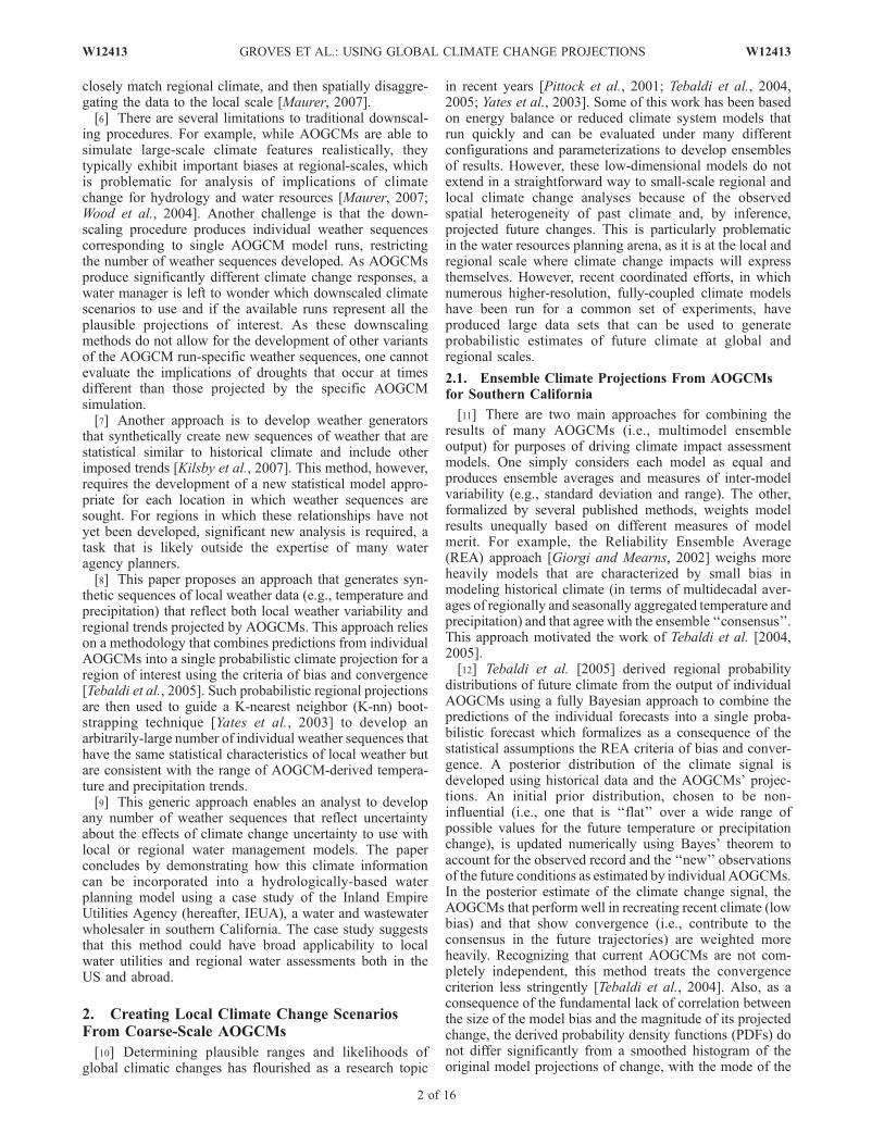
and August) temperature change (in degrees C) and winter(December, January, and February) precipitation change (inpercent precipitation change) from the baseline period(1980–1999) to 2030. The individual changes as estimatedby each AOGCM are indicated by a triangle on the x-axis(biases of the individual models used in the Bayesian

Figure 1. Probability density function of summer temperature change between 2000 and 2030 for theA1B SRES scenario and the southern California region. Points on the curve refer to the deciles of thePDF. Triangles indicate trends from the individual AOGCMs.

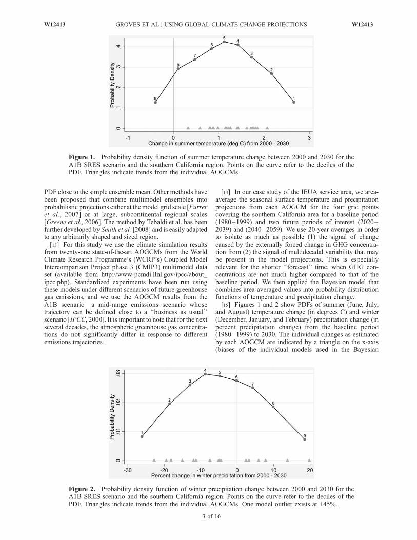
Figure 2. Probability density function of winter precipitation change between 2000 and 2030 for theA1B SRES scenario and the southern California region. Points on the curve refer to the deciles of thePDF. Triangles indicate trends from the individual AOGCMs. One model outlier exists at +45%.

W12413 GROVES ET AL.: USING GLOBAL CLIMATE CHANGE PROJECTIONS

3 of 16

W12413

analysis—which are not correlated to the projected changesreflected in the PDFs—are shown in Figure 3). Figure 1shows a range of projected summer temperature changebetween slightly below zero to over two degrees Celsius.The winter precipitation changes predicted by the individualAOGCMs range from a 25% decrease to a 20% increase(although there is one outlier result that projects a 45%increase). The resulting densities indicate a stronger con-sensus of drier winter conditions relative to the currentclimate. The outcome of the combined AOGCM projectionsfor precipitation change is typical of many regions, partic-ularly in mid-to-low latitudes, where there is low agreementamong the different models [IPCC, 2007b].[16] Note that the Bayesian model is run separately for

both precipitation and temperature, and does not providejoint probabilistic projections. A regression analysis of16 AOGCM projected annual temperature and annualprecipitation trends over the study area from 2005–2050(for the A1b emissions scenario) shows a weak, statisticallyinsignificant negative correlation (p = 0.323). When two ofthe 16 temperature trend and precipitation trend pairs areexcluded, however, the negative relationship become highlysignificant (p = 0.000). Following this suggestive evidence,we assumed that temperature and precipitation trends willbe negatively correlated, and so the driest (wettest) range ofthe precipitation trends corresponds to the warmest (coolest)temperature trends. This assumption is conservative, in thatit will lead to the most inclusive set of plausible climatescenarios as a basis of testing the water-management plansof the IEUA region.

2.2. Generating Local Climate Sequences From theRegional Densities Using K-nn

[17] We next use these regional climate change distribu-tions to develop information relevant for a regional waterresource planning model. The technique presented here usesthe output from the Bayesian method to condition a K-nearestneighbor (K-nn) resampling scheme that generates dailyweather sequences yielding ensembles of alternative climatedata [Yates et al., 2003]. The K-nn algorithm produces dailyweather variables at multiple stations within the regioncovered by the AOGCM grid boxes used to develop thetrend distribution. The derived weather sequences preservethe spatial and temporal dependencies and important crosscorrelations and autocorrelations of the local historicalweather while reflecting large-scale climate trends from theBayesian model. This technique allows for the creation ofensembles of local climate scenarios that can be used in awater planning model for addressing the potential impacts ofclimate change and climate variability, placed within anuncertainty analysis framework.[18] K-nn creates new, synthetic weather sequences by

resampling the historic daily data set in such a way that thestatistical properties of the observed weather data arepreserved. The K-nn Step 1 selects a random startingcalendar day; say a 1 January from all N available 1 January.Step 2 defines a window of days, w to the left and right ofthe starting day selected in Step 1, and aggregates the dailyweather station data into a regional mean. The regionalmean is used to find candidate days similar to the daychosen in Step 1, where similarity is based on a Mahala-nobis distance measure (see Yates et al. [2003] for details).

Figure 3. AOGCM model biases in terms of (left) summer (JJA) average temperature (in degreescentigrade) and (right) winter (DJF) average precipitation (in percentage difference from currentobservations). The asterisks indicate the three models that are used only for the temperature analysis.

4 of 16

W12413 GROVES ET AL.: USING GLOBAL CLIMATE CHANGE PROJECTIONS W12413

With a window width of w = 7 and a data set with N =24 years, the total number of candidate days then givenas k =

ffiffiffiffiffiffiffiffiffiffiffiffiffiffiffiffiffiffiffiffiffiffiffiffiffiffiffiffiffiffiffiffiffiffiffiffiffiffi2wþ 1ð Þ � N½ � � 1

por k = 19 [Rajagopalan and

Lall, 1999]. One of the k similar days is then randomlyselected (Step 3), and represents a day similar to 1 Januaryselected in Step 1. The subsequent day to this selected day isused as the successor, leading to a new 2 January (Step 4).The window of days is then shifted one day to the right, andSteps 2 through 4 are repeated. Successive iterations of thesesteps then generate new, unique daily time series that havemany of the same statistical properties such as autocorrela-tion, cross-covariance, and mean value as the original data[Yates et al., 2003].[19] To reflect a changing climate, as suggested by the

Bayesian climate trends, the pool of ‘‘similar days’’ fromwhich the next day is selected can be biased to include morewarm/cold or wet/dry days. Biased resampling requires aconditioning criterion to select a subset of years, n 2 N, thatwill be used in the K-nn algorithm. The simplest criterionwould be some large-scale climate signal such as the ElNino/Southern Oscillation (ENSO) index, where only yearswith a particular ENSO attribute would comprise the n 2 Nsubset (e.g., only resample from days of daily data). Thisapproach would work fine for short weather sequences,such as a year; but for longer sequences, it would bedesirable to dynamically select an n subset from thepopulation of N years so that longer weather sequencecould reflect different climate regimes. To do this, atemporal, probabilistic resampling scheme is introducedthat generates a subset of days for each week w of year twhose days have a higher or lower probability of beingselected based on a weighting criterion.[20] The weighting criterion is based on a table of weekly

climate anomalies, estimated from historic climate data.These weekly anomalies are assigned a ranked index, Iw

N,for all weeks w and years N. Table 1 shows an example ofthis ranking using precipitation data from the IEUA servicearea (from 1980 to 2003), where regional precipitationanomalies are ranked from driest to wettest. For example,in the 24 years of observational data, the driest week 1 (e.g.,the period 1 through 7 January) was 1981, while the wettestweek 1 was 1995. The driest week 2 was the year 1983,while the wettest week 2 was 1993; and so on.[21] To generate the nw

t subset, an index function is usedto randomly generate indices ranging from i = 1 to N,

I iw ¼ INT N 1� udiw

� �h iþ 1 ð1Þ

where u is a uniform random number, U(0, 1) and dwi is a

weighting parameter that is used to bias years in the rankedlist. In Table 1, years are ranked from driest, with an indexvalue of 1, to wettest, with an index value of N. A weightparameter, dw

i = 1.0, means each year has an equal proba-bility of making up the nw

t subset, values greater than 1.0will tend to bias the selection of wet years, while weightparameter values less than 1.0 will tend to bias dry years.The weight parameter, dw

i of equation (1) can be estimatedboth by week (intra-annual change) and by year (inter-annual change). With a given set of dw

i weights, equation (1)can be randomly queried, leading to a set of indices thatcorrespond to particular years from the ranked list. Finally,this yields a set of biased years, nw

t from which K-nn canresample.[22] The AOGCM-based Bayesian estimate of changes in

seasonal precipitation (DP 0si) and temperature (DT 0

si) for

southern California were linearly interpolated into weeklytime series, DP 0

wi and DT 0

wi from 2000 to 2060. These

interpolations were made for the nine discrete intervals andfor each of the four seasons (see Figures 1 and 2). Thesewere then used to establish the weighting parameter, dw

i forconditioning K-nn, where dw

i = awDP 0wi + bwDT 0

wi . The

aw and bw coefficients were determined by trial-and-error tominimize the difference between the Bayesian estimates ofclimate change and the difference between the futuresynthetic climate and the mean regional climate from thehistoric record. For precipitation, this can be expressed as,

min DP 0is � 1

K

XKi¼1

P_i

s� P_os

!" #ð2Þ

where the regional mean total precipitation for year i andseason s is:

P_i

s ¼1

m

Xmj¼1

P_i

j;s ð3Þ

and P_

j,si is the season total precipitation for station j and year

i; while P̂os is the seasonal station mean computed from theobservations. The total number of stations is m and K is thenumber of synthetic sequences generated by K-nn. Figure 4shows the final weights, dw

i , and the corresponding changein precipitation from the Bayesian model for two selectdeciles: 2 and 8.[23] For the case of the IEUA, N = 24 years of daily

weather data (1980 through 2003) for m = 11 stations wereused to generate biased daily weather sequences with K-nn,conditioned off the results from the Bayesian analysis[Thornton et al., 1997]. For nine deciles of the distributionsshown in Figures 1 and 2, 20 realizations were made leadingto a total of 180, 60-year time series. Note that realizationsare assigned a decile based on the temperature and precip-itation trend applied in the conditioning. Because of thestochastic factors in the K-nn analysis, the precipitation andtemperature trends for individual realizations may notalways order according to a decile. For example, somedecile 3 realizations may have larger temperature trendsthan some deciles 2 realizations.[24] Figures 5 and 6 compare the K-nn simulated data,

the AOGCM ensemble results, and the historical data for

Table 1. A Portion of the Ranked List of Regional Precipitation

Anomalies by Week and Yeara

CategoricalYear Iw

N Week 1 Week 2 . . . Week 52

1; dry Year 1 1981 1983 . . . 19802; dry Year 2 1983 1984 . . . 1985. . . . . . . . . . . . . . . . . .N; wet Year 24 1995 1993 . . . 1994

aSee text for details.

W12413 GROVES ET AL.: USING GLOBAL CLIMATE CHANGE PROJECTIONS

5 of 16

W12413

three discrete deciles (1, 5 and 9) of the Bayesian trenddistributions for winter precipitation and season tempera-ture. The data from the entire historical period can besummarized as a single box plot, which is shown on theleft portion of the graph as total seasonal precipitation(Figure 5) and temperature (Figure 6) averaged over theregion. These box plots represent the range of precipitationand temperature present in the sample of historical data, andshould be compared with box plots to the right thatsummarize each year of simulated data. Linear and non-linear (e.g., loess—see Cleveland and Devlin [1988]) trendsin the historical data indicate a decrease in winter precipi-tation and an increase in summer temperatures throughoutthe brief historical period.[25] The right portion of each figure includes box plots

that summarize the simulated data for precipitation andtemperature for a select set of deciles. Each individual boxplot summarizes all 20 realizations created for a given year.The variance within these values is approximately equivalentto that of the historical data. The thick, light lines in thefigures depict the linear trend from the Bayesian analysis,while the dark line is the mean of all 20 realizations.

Values of dwi were chosen so these lines closely matched

(e.g., the minimization expressed in equation (2)). Notethat decile 1 corresponds to the ‘‘very-warm and dry’’scenarios, while decile 9 are the ‘‘warm and wet’’ scenarios.Also worth noting, the variance within each simulatedseries remains about constant throughout each time seriesrealization.[26] Figure 7 shows three representative sequences of

summer temperature and winter precipitation from 1980 to2060. The data from 1980 to 2003 are based on historicaldata. The data from 2004 to 2060 are based on threerealizations of the K-nn procedure, corresponding to a rangeof conditioning trends.

3. Utilizing the Local Weather Sequences in aWater Management Model

[27] The local weather sequences created using theBayesian-K-nn method can be used with an integrated waterresource management (IWRM) model to evaluate the im-pact of climate change on a water management system. Theliterature is rich with IWRMs that have tended to focus on

Figure 4. (Left) Percentage change in precipitation for (top) decile 2 and (bottom) decile 8 and the(right) final weights used by K-nn to condition the resampling process by month (vertical axis) and year(horizontal axis).

6 of 16

W12413 GROVES ET AL.: USING GLOBAL CLIMATE CHANGE PROJECTIONS W12413

either understanding how water flows through a watershedin response to hydrologic events or on allocating the waterthat is available in response to those events. The WaterEvaluation and Planning Version 21 (WEAP) IWRM (avail-able from http://www.weap21.org) attempts to address thegap between water management and watershed hydrologyby integrating a range of physical hydrologic processes,including rainfall-runoff and snow physics, with the man-agement of demands and installed infrastructure by simulat-ing the water balance for a user-constructed, link-and-noderepresentation of a water management system [Yates et al.,2005a, 2005b]. WEAP allows for multiple-scenario analysis,reflecting uncertainty about climate change and anthropo-genic stressors, such as land use variations, changes inmunicipal and industrial demands, alternative operatingrules, and points of diversion changes. Of particular interestto this study, WEAP can evaluate the impact of alternativesequences of local weather conditions (e.g., temperature,precipitation, humidity, and wind speed) on soil moistureand irrigation requirements, surface and subsurface rainfall

runoff, and percolation of precipitation and irrigation intoaquifers. The WEAP IWRM has been applied to numerouswatersheds and districts throughout the world, including theSacramento Valley, in California [Yates et al., 2008]. Huber-Lee et al. [2006] provide additional background on WEAPand present three municipal water case study applications.

4. A Case Study of the Inland Empire UtilitiesAgency in Southern California

[28] To demonstrate how the climate change data derivedfrom the Bayesian-K-nn approach described above can beutilized in a water planning model to inform water planningdecisions, we present a case study focused on the servicearea of the Inland Empire Utilities Agency (IEUA), awholesale water and wastewater provider in RiversideCounty, southern California (Figure 8). This analysis rep-resents a subset of work performed in collaboration withIEUA staff members and focuses on illustrating the range ofimpacts that climate may have on the water system. Workexamining new approaches to interpreting this information

Figure 5. Winter precipitation (December, January, and February) for the historic period (1980 through2003) with a (left graph) trend and loess lines and summarized as a (far left) box plot. Right portion ofgraph are the K-nn simulated time series of annual precipitation, given as box plots for all realizations (K =20). The thick, light-colored line is the AOGCM ensemble climate change estimate relative to the historicmean.

W12413 GROVES ET AL.: USING GLOBAL CLIMATE CHANGE PROJECTIONS

7 of 16

W12413

for decision making is presented by Groves et al. [2008a,2008b].[29] The IEUA region is in the midst of rapid urban

growth and transformation from an agricultural region dom-inated by dairy farms to industrial and planned residentialdevelopments. It is projected that the region’s population of800,000 will grow to approximately 1.2 million by 2025,placing new demands on the water supply and wastewatertreatment system [IEUA, 2005].[30] The IEUA region currently meets slightly more than

half of its average water needs from groundwater sourceswithin the region (primarily the underlying Chino Ground-water basin aquifer), about a quarter from Northern Cal-ifornia via a large intra-state water distribution system (i.e.,the California State Water Project), and the rest from localrivers and streams and a rapidly expanding recycled watersystem [IEUA, 2005]. The Chino Groundwater basin wasadjudicated in 1978 [Chino Basin Municipal Water Districtv. City of Chino, 1978] and is managed to maximizesustainable extractions of groundwater according to theChino Basin Optimum Management Program (OBMP)

[Wildermuth Environmental, 1999]. Two key componentsof the groundwater program are (1) a comprehensiveprogram to replenish the groundwater basin with imported,recycled, and local storm water and (2) limitations onextractions to ensure long-term sustainability. The manage-ment plan stipulates that allowable extractions will beadjusted over time to respond to changing groundwaterconditions.

4.1. Plausible Impacts of Climate Change to theIEUA Region

[31] A simple qualitative assessment of the region’ssystem would suggest that climate change has the potentialto impact water supply reliability by increasing irrigationdemands, decreasing the natural recharge of the groundwa-ter basin that would lead to more stringent restrictions ongroundwater use, decreasing local runoff and derived mu-nicipal supplies, and reducing the availability of importedwater from Northern California.[32] To quantitatively assess the ranges of plausible

impacts that climate change may have upon water manage-

Figure 6. Same as Figure 5 but for average summer temperature (June, July, and August).

8 of 16

W12413 GROVES ET AL.: USING GLOBAL CLIMATE CHANGE PROJECTIONS W12413

ment in the IEUA service area, we developed a WEAPmodel that estimates the performance of IEUA’s watermanagement strategies under each of the future weathersequences produced by the Bayesian-K-nn procedure

described above. To automate the generation and manage-ment of a large number of WEAP simulations correspondingto the developed climate change weather sequences (orscenarios), we used the Computer Assisted Reasoning system(CARsTM), available from Evolving Logic (www.evolvinglogic.com).[33] The WEAP model was designed to produce under

nominal assumptions results that are consistent with thevarious IEUA estimates of water demand and supplyincluded in the IEUA 2005 Regional Urban Water Man-agement Plan (hereafter, IEUA RUWMP) [IEUA, 2005].The WEAP model necessarily simplifies a complex watermanagement system and thus assessed climate impacts maybe biased. The ultimate purpose of the analysis, however,was to develop and illustrate new approaches for addressingclimate uncertainties in water planning—not necessarily todevelop the most comprehensive or accurate model repre-sentation of the case study area.[34] The WEAP model simulates water supply and

demand using a stylized representation of the major waterflows of the system on a monthly time scale from 2005 to2040. The model represents supply and demand relation-ships by using a set of nodes corresponding to discretewater management elements such as catchments, indoor-demand sectors, surface supplies, and groundwater basins.These elements are linked together by rivers, conveyancefacilities, and other pathways (such as percolation flows).[35] The model includes a simple representation of the

Chino Groundwater basin aquifer in which ‘‘effective safeyield’’ for pumping and direct use is endogenously calcu-lated at 5-year intervals throughout the simulation such thatgroundwater inflows (e.g., percolation from overlyingcatchments and replenishment by imported, recycled, and

Figure 7. Representative temperature and precipitationsequences for the IEUA region derived using K-nnconditioned to recreate the extremes of the regional trendPDFs.

Figure 8. Map of the IEUA service area, California, USA. The city of Ontario is located at 34�N,117�410W.

W12413 GROVES ET AL.: USING GLOBAL CLIMATE CHANGE PROJECTIONS

9 of 16

W12413

local storm water) are balanced with outflows (e.g., pumpedwater for treatment and direct use). The time series ofmonthly weather parameters drive the system’s hydrologyvia a soil-moisture model embedded in WEAP. The specificmodel specification was based on the IEUA RUWMP,Chino Basin Optimum Management Program [WildermuthEnvironmental, 1999], and other regional studies [e.g.,Husing, 2006].[36] Model calibration consisted of four main tasks:

(1) tuning WEAP parameters so that modeled demand underhistorical climate and projected land-use and demographicassumptions match the demand forecast reported in theIEUA RUWMP; (2) tuning the Chino Basin catchmentparameters so that percolation of historical precipitationand planned groundwater replenishment leads to the totalbasin inflow required to balance extractions according to theChino Basin Peace I agreement [Chino Basin Watermaster,2000]; (3) tuning Metropolitan import parameters so thatperiods of dry years trigger expected shortfalls in importdeliveries; (4) tuning the upper catchment and local riverflow so that local supplies vary with precipitation within thehistorical range described in the IEUA RUWMP. Pleaserefer to the study of Groves et al. [2008a, 2008b] for detailson model specification and calibration.[37] On the basis of the modeling specification, the

pathways through which climatic change can affect watermanagement conditions in the IEUA region are: (1) irriga-tion requirements, (2) rates of groundwater infiltration,(3) availability of local supplies for direct use and ground-water replenishment, and (4) availability of importedsupplies for direct use and groundwater replenishment.The subsections below describe the range of plausibleclimate change impacts upon the IUEA water management

system derived from the global climate models via theBayesian-K-nn methodology.4.1.1. Outdoor Irrigation Demands[38] Changes in precipitation and temperature will affect

outdoor irrigation demand. WEAP computes irrigationrequirements for each catchment (e.g., contiguous regionwith similar hydrologic characteristics) by using a soilmoisture algorithm [Yates et al., 2005a, 2005b] that factorsin monthly temperature and precipitation, crop moisturerequirements (parameterized by a crop coefficient), surfacerunoff characteristics, soil water capacity and conductivity,and bulk parameters that specify when irrigation water isneeded as a function of soil moisture. This formulationspecifies that increased air temperature leads to higherpotential evapotranspiration (PET) rates and greater land-scape water needs. There are other potentially importanteffects that climate could have upon evapotranspiration notconsidered by the WEAP model, such as temperature effectson crops and their growing season [Lobell et al., 2006] andeffects of CO2 on crop photosynthesis [Kimball et al.,2002].[39] Figure 9 shows traces of outdoor urban irrigation

demand (including domestic and commercial landscaping),averaged over 20 weather sequences for five differentclimate trends (corresponding to climate change deciles 1,3, 5, 7 and 9), assuming that all other 2005 conditionsremain constant (e.g., land use patterns, demand factors, andwater supply variability). The gray bars indicate the rangesof outdoor demand by year for all 180 sequences reflectiveof all nine climate change deciles. The figure suggestsincreased water demands under hotter and drier weatherprojections (up to an 11% increase by 2040, or an increaseof 0.28 centimeters per year for decile 1) and significantlylower water demand under the wetter weather sequences (up

Figure 9. Projected outdoor water demand (in centimeters per year) for the IEUA region under differentweather sequences consistent with the climate change projections from the AOGCMs. The lines indicateaverages over 20 sequences for deciles 1, 3, 5, 7, and 9. The shaded bars indicate the entire range ofannual demand per year. Note that the deciles are defined based on the conditioning precipitation andtemperature trends used in the K-nn procedure. They are not defined based on the output data shown hereand thus will not always order according to decile.

10 of 16

W12413 GROVES ET AL.: USING GLOBAL CLIMATE CHANGE PROJECTIONS W12413

to a 10% decrease by 2040, or a decrease of 0.33 centi-meters per year for decile 9). The interannual variabilityreflected by the ranges of all annual demand projections issubstantially larger than the average trends in demand. Notethat in the IEUA region, these climate-induced trends wouldbe superimposed upon rising urban water demands becauseof projected landscape conversion from agricultural landsand open space to urban development.4.1.2. Local Supplies[40] Trends in precipitation will change the availability of

local stream flow for municipal supplies. Although a WEAPmodel could be constructed to explicitly model runoff tothese local waterways, this application parameterizes thestream flow that are the source of local surface water supplysuch that during low precipitation years (as defined by theweather sequence being used) a lower supply is availablefor direct use and groundwater replenishment. This param-eterization is tuned so that historical precipitation sequen-ces lead to local supply availability commensurate withthat observed historically (about 20 million m3/year, onaverage).[41] Figure 10 shows traces of local surface supplies,

averaged over 20 sequences for five different climate trends(deciles 1, 3, 5, 7 and 9). The gray bars indicate the rangesof local surface supply by year for each of the 180sequences representative of the nine climate change deciles.The range of local surface supplies for the derived weathersequences suggests decreased supplies under hotter anddrier weather projections (substantial supply decreases of42% by 2040—191 thousand m3/year for decile 1) andgreater supplies under the wetter weather sequences (up to a42% increase by 2040—199 thousand m3/year for decile 9).The interannual variability reflected by the ranges of all 180local supply projections is substantially larger than theaverage trends in the local supply by decile.

4.1.3. Groundwater Infiltration[42] Trends in precipitation could change the amount of

precipitation that percolates into the underlying aquifer. TheWEAP model calculates the share of monthly precipitationthat (1) is evapotranspired by the land surface; (2) flows offof the catchment surface into surface streams; (3) percolatesinto the root-zone and flows laterally to adjacent surfacestreams; and (4) percolates from the root-zone into theunderlying aquifer. Precipitation that percolates beyondthe root zone is the primary source of inflow to theunderlying Chino Groundwater basin aquifer. Groundwaterreplenishment using imported, recycled, and local stormwater via percolation is also simulated. The model structureassumes that percolation is linearly related to precipitation.[43] To evaluate the effects of climate change on the

groundwater basin management, we simulated how the180 climate sequences affect the Chino Basin storageassuming that development and water management patternsunfold as projected in the IEUA RUWMP (Figure 11). Inthese simulations the management of the Chino Basin isfixed—it does not respond to rising or declining groundwa-ter levels. The climate sequences that exhibit positive trendsin precipitation lead to increasing groundwater storage, andthe climate sequences with negative precipitation treads leadto decreases in groundwater storage. Groundwater levelsdecline by about 15% (or 950 million m3/year) under decile1 climate sequences and increase by 13% (or 789 million m3/year) under decile 9 climate sequences over the 35-yearsimulation period.[44] Per the OBMP, groundwater extractions would be

limited if the amount of water stored in the aquifer were tosignificantly decline. To evaluate how changes in pumpingpermits to ensure sustainability would affect overall ground-water extractions under the various climate change scenarios,the model adjusts groundwater extractions every 5 years so

Figure 10. Projected local surface supply (in million cubic meter per year) for the IEUA region underdifferent weather sequences consistent with the climate change projections from the AOGCMs. The linesindicate averages over 20 sequences for deciles 1, 3, 5, 7, and 9. The shaded bars indicate the entire rangeof local supply availability. Note that the deciles are defined based on the conditioning precipitation andtemperature trends used in the K-nn procedure. They are not defined based on the output data shown hereand thus will not always order according to decile.

W12413 GROVES ET AL.: USING GLOBAL CLIMATE CHANGE PROJECTIONS

11 of 16

W12413

that total groundwater storage remains at the current level(about 6.2 trillion m3). Figure 12 shows the projectedextractions under the IEUA RUWMP assumptions (solidline) and average extractions by year for the weather sequen-ces corresponding to climate change deciles 1, 3, 5, 7, and 9.The shaded region represents the range of all simulations.Declines in supply are due to projected groundwater pumpingreductions mandated in response to falling groundwater

levels. Note that restrictions are enacted or eased every fiveyears, per the OBMP. These simulations suggest that undermore severe climate change scenarios (i.e., lower climatechange deciles) significant declines in allowable groundwa-ter extractions could be mandated. Specifically, the averagerestrictions under deciles 1 and 3 after 2010 (when the modelfirst evaluates the condition of the groundwater basin andadjusts allowable extractions as needed) is 30.8 million m3/year

Figure 11. Chino Basin groundwater storage projections (trillion cubic meter) assuming no change inmanagement under different weather sequences reflective of climate deciles 1, 3, 5, 7, and 9. Linesindicate averages across 20 sequences for each decile. The shaded region indicates the range of resultsacross all 180 sequences (20 sequences for each of the 9 deciles). Note that the deciles are defined basedon the conditioning precipitation and temperature trends used in the K-nn procedure. They are notdefined based on the output data shown here and thus will not always order according to decile.

Figure 12. Projections of allowable groundwater extractions (million cubic meter) from the ChinoBasin under climate change scenarios and adaptive groundwater management. The lines indicate averageextractions (across 20 sequences) for deciles 1, 3, 5, 7, and 9. Shaded region indicates the range of resultsfrom the 180 sequences. Note that the deciles are defined based on the conditioning precipitation andtemperature trends used in the K-nn procedure. They are not defined based on the output data shown hereand thus will not always order according to decile.

12 of 16

W12413 GROVES ET AL.: USING GLOBAL CLIMATE CHANGE PROJECTIONS W12413

(or 14% of the total groundwater supply) and 17.3 millionm3/year (or 8% of the total), respectively. Restrictions underindividual plausible weather sequences are even moresignificant, as seen by the range results in Figure 12.4.1.4. Imports[45] The amount of imported supply available to IEUA

will also likely be affected by changed climatic conditions inthe Sacramento Valley (the source region of the CaliforniaState Water Project) [Barnett et al., 2008; Department ofWater Resources, 2006; Vicuna, 2006; Zhu et al., 2005]. Asthis case-study did not explicitly model the hydrologicresponse of the Sacramento Valley river flow to climatechange, we evaluate the effects of various reductions inavailable imports on the water management implicationssection below.

4.2. Implications for Current Management Plans

[46] We now address the question of how climate changeimpacts will affect the overall performance of the IEUA’swater management plans. Specifically, we present howplausible climate changes, as suggested by the 21 AOGCMsand translated into local temperature and precipitationsequences using K-nn, would affect the performance ofthe region’s current plans (i.e., the IEUA RUWMP; IEUA[2005]) under several levels of decline in imported supplyavailability. It is important to note that this approach doesnot explicitly consider uncertainties associated with thedownscaling procedure or hydrologic modeling routinesused by the WEAP model.[47] The IEUA RUWMP’s primary approach to address-

ing new water supply needs includes (1) increasing the useof the Chino Basin groundwater by about 75% throughincreased groundwater replenishment and (2) developing anextensive recycled water system to deliver up to 85 millionm3/year of supply by 2025 (2005 recycled deliveries totaledonly about 9.9 million m3). To summarize the effects thatclimate change would have on the performance of theregion’s plans with respect to supply and demand, theWEAP model calculates the average annual surplus (de-fined as the difference between total available water supplyand total water demand) from 2021–2030 and from 2031–2040. Annual reliability is also calculated by counting thefraction of years in which the surplus is negative andsubtracting that from one. Note that according to the IEUARUWMP, the region would enjoy an excess of availablesupply that would grow from 17.9 million m3 in 2005 to101.3 million m3 by 2025 under historical conditions.[48] As this model does not explicitly evaluate the climate

change impacts on the SWP source regions, we calculate theperformance of the IEUA RUWMP under the 180 weathersequences (reflecting local changes in climate) for threelevels of fixed imports: current projections, a 20% declineby 2040, and a 40% decline by 2040. These three levelswere selected to represent the range of declines suggestedby several recent studies that estimated the reliability ofSWP deliveries under different climate change scenarios[Department of Water Resources, 2006; Vicuna, 2006; Zhuet al., 2006]. Note that annual imports are also restrictedduring local-dry years according to the IEUA RUWMPprojections for single-dry year SWP deliveries to the region.[49] Under no climate trends and no declines in imports

the average surplus is about 88.8 million m3 between 2021and 2030 and 82.6 million m3 between 2031 and 2040 (top

line of Table 2), and reliability is estimated to be 100%.Under declining average imports, however, the averagesurplus decreases to 61.7 million m3 in 2030–2040 for20% import declines and 34.5 million m3 in 2030–2040 fora 40% decline in imports. Reliability decreases to 96%.[50] Under the sequences in which precipitation increases

on average (deciles 7 and 9), conditions are as good as orbetter than under those without climate trends (Rows 5and 6). In these cases, increases in precipitation offset thewarming increases projected under deciles 7 and 9. Decile 5,which exhibits a slightly declining precipitation and temper-ature increases, leads to worsening conditions for the IEUAservice area when compounded with declines in imports. Inthe 2031–2040 time period with 20% declines in imports,the average surplus decreases by 21.0 million m3 andreliability decreases to 96%. Under a 40% decline in imports,average surplus decreases to 6.8 million m3 by the 2031–2040 time period and reliability decreases to 78%. Underclimate changes consistent with deciles 3 and 1, the regionexperiences reduced reliability and significantly lower aver-age surpluses even when there are no declines in imports. Bythe 2031–2040 time period, the region’s supply buffer iseliminated regardless of the effects on MWD imports, andreliability decreases to less than 40% under the 20% and40% declines in imports.

5. Summary and Discussion

[51] This paper describes a methodology for developingsequences of monthly local weather data that reflect region-al climate trends as projected by global climate models.These sequences provide a quantitative representation ofplausible climate change impacts and can be used by watermanagement models to stress test water management plans.[52] The methodology first develops PDFs of temperature

and precipitation trends for a region from individualAOGCM results using the criteria of bias and convergence[Tebaldi et al., 2005]. It then creates sequences of localweather using the K-nn bootstrapping technique [Yates etal., 2003] that resamples daily historical weather data suchthat the future sequences have the same statistical character-istics of local weather but are consistent with the range ofAOGCM-derived temperature and precipitation trends. Thismethod overcomes the limitations accompanying an analy-sis that uses individual, nuanced AOGCM runs. Utilizingnumerous sequences with similar underlying climate trendscan be useful, as the timing and duration of droughts canmake the difference between successful and unsuccessfullong-term water management strategies.[53] A key limitation of the K-nn approach as imple-

mented here is the challenge to estimate the weightingparameter, dw

i , that correctly biases the new weather sequen-ces to properly reflect the AOGCM ensembles both sea-sonally and inter-annually. This is currently done manually,through trial-and-error. The applied method also does notguarantee that all climate impacts are accounted for nor thatall possible uncertainties are addressed.[54] The method described here provides data to support

a climate impact assessment. A common approach is toevaluate management strategies against a few projections ofaltered climatic conditions (often including ‘‘bookend’’projections). Bookend climate projections can be useful toillustrate the range of possible outcomes, but they do not

W12413 GROVES ET AL.: USING GLOBAL CLIMATE CHANGE PROJECTIONS

13 of 16

W12413

provide water managers with information about how muchclimate change a water agency can reasonably accommo-date under different management strategies, for example.[55] Water planners also face other important uncertainties

about future conditions, and the derived climate sequencescan also be combined with other assumptions about uncertainplanning conditions to develop numerous scenarios. Asystematic evaluation of these scenarios can help answerquestions such as: ‘‘How bad must climatic changes bebefore our agency should invest in some new infrastructureor implement a particular water efficiency program?’’ and‘‘What conditions would need to prevail for me to wish Ihad made alterative strategic decisions?’’[56] A key challenge is how to use these large ensembles

of scenarios in a systematic decision analysis. Standarddecision theory would call for the assignment of probabil-ities to each scenario and weighting of the results. Such anapproach could lead to the identification of ‘‘optimal’’ watermanagement strategies (provided that a single utility func-tion could be defined). When the uncertainty about thefuture cannot be uniquely characterized by probabilisticmeans, however, alternative decision analytic methodsmay be required [Groves and Lempert, 2007; Grubler andNakicenovic, 2001; Hall, 2007; Lempert et al., 2004; New etal., 2007; Wack, 1985].[57] In the case of long-term water planning in the IEUA

region, the cascading uncertainty from global greenhousegas emissions estimates, to the global and regional climateresponse, to the local, downscaled hydrological response,makes it difficult to assign credible probabilistic uncertaintycharacterizations to changes in precipitation and tempera-ture in the IEUA region and the source region of itsimported supplies. Uncertainty about other managementconditions, such as the ability for the region to aggressivelyexpand its recycled water system, also cannot be easilycharacterized.[58] Under conditions of so-called ‘‘deep uncertainty’’ the

identification of robust solutions may be a more fruitfulpursuit. Robust decision making (RDM) [Groves andLempert, 2007; Lempert et al., 2003, 2006] is a structured,scenario-based analytic approach for identifying solutionsthat perform adequately across a wide range of plausiblefuture conditions. In brief, RDM first evaluates the per-

formance of different strategies against a large set ofscenarios. RDM then analyzes the resultant database usingvisualization and statistical techniques to identify condi-tions under which the leading strategies perform poorly.Identifying alternative strategies that are insensitive tothese vulnerabilities can then help develop hedging actionsto augment the promising strategies. Note that it iscommon to factor in cost when estimating how well apolicy will fare, thus robust policies are not necessarilythose that cost more. In the end, no strategy can be robustto all possible future conditions. The characterizations ofvulnerabilities then provide decision makers with keytradeoff information to help them understand how adiffering world view about critical uncertainties (such asclimate change effects) would impact sensible choices.[59] In this paper, the case study evaluates the implica-

tions of 180 different weather projections upon IEUA’scurrent urban water management plan. The results showedthat under drying climate sequences, outdoor water demandcould increase substantially at the same time as local surfacewater supplies and groundwater resources become moreconstrained. Together, the effects would lead to reductionsin the planned supply buffer and possible shortages. Com-pounding these local effects with declines in imports (drivenby climate change or other factors in the imported watersource region) would impacts IEUA water managementeven more.[60] Groves et al. [2008a, 2008b] build on this analysis

and evaluate how alternative management strategies for theIEUA region would perform against this range of plausibleclimate changes and other management uncertainties. Theirrobust decision making analysis finds that much of theIEUA region’s vulnerability to climate change could bereduced by more aggressive promotion of water use effi-ciency in the near-term and investments in storm watercapture for groundwater recharge if conditions deteriorateover the long-term. These strategies prove to be more robustthan IEUA current plans because the cost of new invest-ments are outweighed in a vast majority of the conditionsevaluated by reductions in costly shortages and through thereduction in use of expensive imported supplies.[61] These results were shown to stakeholder groups

consisting of water managers and elected officials from

Table 2. Average Annual Surplus (in Million Cubic Meter) and Reliability (%, See Key) Under Different Climate Change Trends

(Rows), Trends in Imports (Major Columns), and Time Periods (Minor Columns)

ClimateChangeTrend

Average Annual Surplus (million m3) and Reliability (see key)

No Decline in Imports 20% Decline in Imports by 2040 40% Decline in Imports by 2040

2021–2030 2031–2040 2021–2030 2031–2040 2021–2030 2031–2040

No climate trend 89.2 82.8 75.5 62.0 60.8 33.9a

Decile 1 35.5a �12.3b 20.1a �55.5d 0.2b �115.0d

Decile 3 47.1a 41.1a 31.2a 13.4a 14.2b �31.5c

Decile 5 76.8 62.7 63.2 40.7a 47.2a 6.8b

Decile 7 89.7 78.8 76.4 60.2 61.9 34.0a

Decile 9 109.3 102.3 96.8 83.8 84.2 65.3

Bold data correspond to a reliability of less than 80%.aReliability range of 80%–100%.bReliability range of 60%–79%.cReliability range of 40%–59%.dReliability range of less than 40%.

14 of 16

W12413 GROVES ET AL.: USING GLOBAL CLIMATE CHANGE PROJECTIONS W12413

the IEUA region. An analysis of surveys administeredbefore and after the presentations suggests that the partic-ipants are concerned about climate change impacts on theirwater system and that large scenario ensembles evaluatedwith RDM methods can be useful in crafting a prudentresponse.

[62] Acknowledgments. The authors of this report are grateful for thefinancial support received from the National Science Foundation (grantSES-0345925) and from NCAR Weather and Climate Impacts Assessmentprogram. NCAR is sponsored by the National Science Foundation. Theauthors also acknowledge the modeling groups, the Program for ClimateModel Diagnosis and Intercomparison (PCMDI), and the WCRP’s WorkingGroup on Coupled Modelling (WGCM) for their roles in making availablethe WCRP CMIP3 multimodel data set. Support of this data set is providedby the Office of Science, U.S. Department of Energy. This paper reports onwork that received substantive assistance from RAND colleagues RobertLempert, Debra Knopman, Sandra Berry, and Lynne Wainfan. The casestudy analysis would not have been possible without the support of MarthaDavis and Richard Atwater of the IEUA.

ReferencesBarnett, T. P., et al. (2008), Human-induced changes in the hydrology of thewestern United States, Science, 319, 1080–1083.

Brekke, L. D., N. L. Miller, K. E. Bashford, N. W. T. Quinn, and J. A.Dracup (2004), Climate change impacts uncertainty for water resourcesin the San Joaquin River Basin, California, J. Am. Water Resour. Assoc.,40(1), 149–164.

California Urban Water Agencies (2007), Climate Change and UrbanWater Resources, 15 pp., California Urban Water Agencies, Sacramento,CA.

Chino Basin Municipal Water District v. City of Chino et al. (1978), Super-ior Court of the County of San Bernardino, no. 164327, 30 Jan.

Chino Basin Watermaster (2000), Peace Agreement Chino Basin, ChinoBasin Watermaster, Rancho Cucamonga, CA.

Cleveland, W. S., and S. J. Devlin (1988), Locally weighted regression: Anapproach to regression analysis by local fitting, J. Am. Stat. Assoc., 83,596–610.

Department of Water Resources (2006), Progress on Incorporating Cli-mate Change Into Planning and Management of California’s WaterResources—Technical Memorandum Report, California Dept. of WaterResour., Sacramento, Calif.

Fowler, H. J., S. Blenkinsop, and C. Tebaldi (2007), Linking climatechange modeling to impacts studies: Recent advances in downscalingtechniques for hydrological modeling, Int. J. Climatol., 27(12), 1547–1578.

Furrer, R., R. Knutti, S. R. Sain, D. W. Nychka, and G. A. Meehl (2007),Spatial patterns of probabilistic temperature change projections from amultivariate Bayesian analysis, Geophys. Res. Lett., 34, L06711,doi:10.1029/2006GL027754.

Giorgi, F., and L. O. Mearns (2002), Calculation of average, uncertaintyrange, and reliability of regional climate changes from AOGCM simula-tions via the ‘‘reliability ensemble averaging’’ (REA) method, J. Clim.,15, 1141–1158.

Greene, A., L. Goddard, and U. Lall (2006), Probabilistic multimodel re-gional temperature change projections, J. Clim., 19, 4326–4343.

Groves, D. G., and R. J. Lempert (2007), A new analytic method for findingpolicy-relevant scenarios, Global Environ. Change, 17, 73–85.

Groves, D. G., D. Knopman, R. Lempert, S. Berry, and L. Wainfan (2008a),Presenting Uncertainty About Climate Change to Water Resource Man-agers—Summary of Workshops With the Inland Empire Utilities Agency,RAND, Santa Monica, Calif.

Groves, D. G., R. Lempert, D. Knopman, and S. Berry (2008b), Preparingfor an Uncertain Future Climate in the Inland Empire—Identifying RobustWater Management Strategies, RAND Corporation, Santa Monica, Calif.

Grubler, A. N., and N. Nakicenovic (2001), Identifying dangers in an un-certain climate, Nature, 412, 15.

Hall, J. (2007), Probabilistic climate scenarios may misrepresent uncer-tainty and lead to bad adaptation decisions, Hydrol. Process., 21,1127–1129.

Huber-Lee, A., C. Swartz, J. Sieber, J. Goldstein, D. Purkey, C. Young,E. Soderstrom, J. Henderson, and R. Raucher (2006), Decision SupportSystem for Sustainable Water Supply Planning, 67 pp., AWWA ResearchFoundation, Denver, Colo.

Husing, J. (2006), Inland Empire Utility Agency Demand Drivers: 2004 toBuild-Out, 25 pp., Economics & Politics, Inc., Redlands, CA.

Inland Empire Utilities Agency (2005), 2005 Regional Urban Water Man-agement Plan, Inland Empire Utilities Agency, Chino, Calif.

Intergovernmental Panel on Climate Change (2000), IPCC Special Report—Emissions Scenarios, Intergovernmental Panel on Climate Change.

Intergovernmental Panel on Climate Change (2007a), Climate Change2007: Impacts, Adaptation and Vulnerability, Contribution of WorkingGroup II to the Fourth Assessment Report of the IntergovernmentalPanel on Climate Change, edited byM. L. Parry et al., 976 pp., CambridgeUniv. Press, Cambridge, U.K.

Intergovernmental Panel on Climate Change (2007b), Climate Change2007: The Physical Scientific Basis, Contribution of Working Group Ito the Fourth Assessment Report of the Intergovernmental Panel onClimate Change, edited by S. Solomon et al., 996 pp., Cambridge Univ.Press, Cambridge, U.K. and NY.

Kilsby, C. G., P. D. Jones, A. Burton, A. C. Ford, H. J. Fowler, C. Harpham,P. James, A. Smith, and R. L. Wilby (2007), A daily weather generatorfor use in climate change studies, in Environmental Modelling & Soft-ware, pp. 1705–1719, Elsevier, Amsterdam, Netherlands.

Kim, J. W., J. T. Chang, N. L. Baker, D. S. Wilks, and W. L. Gates (1984),The statistical problem of climate inversion: Determination of the rela-tionship between local and large-scale climate, Mon. Weather Rev., 112,2069–2077.

Kimball, B. A., K. Kobayashi, and M. Bindi (2002), Responses of agricul-tural crops to free-air CO2 enrichment, Adv. Agron., 77, 293–368.

Knopman, D. S. (2006), Success matters: Recasting the relationship amonggeophysical, biological, and behavioral scientists to support decisionmaking on major environmental challenges, Water Resour. Res., 42,W03S09, doi:10.1029/2005WR004333.

Lamb, P. (1987), On the development of regional climate scenarios forpolicy oriented climatic impact assessments, Bull. Am. Meteorol. Soc.,68, 1116–1123.

Lempert, R. J., S. W. Popper, and S. C. Bankes (2003), Shaping the NextOne Hundred Years: New Methods for Quantitative, Long-Term PolicyAnalysis, 187 pp., RAND, Santa Monica, Calif.

Lempert, R., N. Nakicenovic, D. Sarewitz, and M. Schlesinger (2004),Characterizing climate-change uncertainties for decision-makers, Clim.Change, 65, 1–9.

Lempert, R. J., D. G. Groves, S. W. Popper, and S. C. Bankes (2006), Ageneral, analytic method for generating robust strategies and narrativescenarios, Manage. Sci., 52(4), 514–528.

Lobell, D., C. Field, K. Cahill, and C. Bonfils (2006), Impacts of FutureClimate Change on California Perennial Crop Yields: Model Projec-tions With Climate and Crop Uncertainties, 25 pp., Lawrence Liver-more Natl. Lab., Livermore, CA.

Maurer, E. P. (2007), Uncertainty in hydrologic impacts of climate changein the Sierra Nevada, California under two emissions scenarios, Clim.Change, 82, 9180–9189.

Miller, K., and D. Yates (2006), Climate Change and Water Resources: APrimer for Municipal Water Providers, 83 pp., American Water WorksAssociation, Denver, CO.

New, M., A. Lopez, S. Dessai, and R. Wilby (2007), Challenges in usingprobabilistic climate change information for impact assessments: Anexample from the water sector, Philos. Trans. R. Soc. London, Ser. A,365, 2117–2131.

Pittock, A. B., R. N. Jones, and C. D. Mitchell (2001), Probabilities willhelp us plan for climate change, Nature, 413, 249.

Rajagopalan, B., and U. Lall (1999), A k-nearest-neighbor simulator fordaily precipitation and other variables, Water Resour. Res., 35(10),3089–3101.

Risbey, J. S. (1998), Sensitivities of water supply planning decisions tostreamflow and climate scenario uncertainties,Water Policy, 1, 321–340.

Schimmelpfennig, D. (1996), Uncertainty in economic models of climate-change impacts, Clim. Change, 33(2), 213–234.

Smith, R. L., C. Tebaldi, D. Nychka, and L. O. Mearns (2008), Bayesianmodeling of uncertainty in ensembles of climate models, J. Am. Stat.Assoc., in press.

Stakhiv, E. Z. (1998), Policy implications of climate change impacts onwater resources management, Water Policy, 1(2), 159–175.

Tebaldi, C., L. O. Mearns, D. Nychka, and R. L. Smith (2004), Regionalprobabilities of precipitation change: A Bayesian analysis of multimodelsimulations, Geophys. Res. Lett. , 31 , L24213, doi:10.1029/2004GL021276.

Tebaldi, C., R. L. Smith, D. Nychka, and L. O. Mearns (2005), Quantifyinguncertainty in projections of regional climate change: A Bayesian

W12413 GROVES ET AL.: USING GLOBAL CLIMATE CHANGE PROJECTIONS

15 of 16

W12413

approach to the analysis of multimodel ensembles, J. Clim., 18(10), 1524–1540.

Thornton, P. E., S. W. Running, and M. A. White (1997), Generatingsurfaces of daily meteorology variables over large regions of complexterrain, J. Hydrol., 190, 214–251.

Vicuna, S. (2006), Predictions of Climate Change Impacts on CaliforniaWater Resources Using CALSIM II: A Technical Note, California ClimateChange Center, Berkeley, CA.

Vicuna, S., E. P. Maurer, B. Joyce, J. A. Dracup, and D. Purkey (2007), Thesensitivity of California water resources to climate change scenarios,J. Am. Water Resour. Assoc., 43(2), 482–498.

Wack, P. (1985), The Gentle Art of Reperceiving—Scenarios: Shooting theRapids (part 2 of a two-part article), Harvard Bus. Rev. (November–December), pp. 2–14.

Wildermuth Environmental (1999), Optimum Basin Management Program—Phase 1 Report, Chino Basin Watermaster, Lake Forest, CA.

Wood, A. W., L. R. Leung, V. Sridhar, and D. P. Lettenmaier (2004),Hydrologic implications of dynamical and statistical approaches todownscaling climate model outputs, Clim. Change, 15(62), 189–216.

Yates, D., S. Gangopadhyay, B. Rajagopalan, and K. Strzepek (2003), Atechnique for generating regional climate scenarios using a nearest neigh-bor algorithm, Water Resour. Res., 39(7), 1199, doi:10.1029/2002WR001769.

Yates, D., D. Purkey, J. Sieber, A. Huber-Lee, and H. Galbraith (2005a),WEAP21—A demand-, priority-, and preference-driven water planning

model. part 2: Aiding freshwater ecosystem service evaluation, WaterInt., 30, 501–512.

Yates, D., J. Sieber, D. Purkey, and A. Huber-Lee (2005b), WEAP21—Ademand-, priority-, and preference-driven water planning model. part 1,Water Int., 30, 487–500.

Yates, D., D. Purkey, J. Sieber, A. Huber-Lee, H. Galbraith, J. West, andS. Herrod-Julius (2008), A physically-based, water resource planningmodel of the Sacramento Basin, California USA, ASCE J. Water Resour.Planning Manage., in press.

Zhu, T., M. W. Jenkins, and J. R. Lund (2005), Estimated impacts ofclimate warming on California water availability under twelve futureclimate scenarios, J. Am. Water Resour. Assoc., 14(5), 1027–1038.

Zhu, T., M. W. Jenkins, and J. R. Lund (2006), Estimated Impacts ofClimate Warming on California Water Availability Under Twelve FutureClimate Scenarios, California Energy Commission, Sacramento, CA.

����������������������������D. G. Groves, RAND Corporation, 1776 Main Street, P.O. Box 2138,

Santa Monica, CA 90407-2138, USA. (groves@rand.org)

C. Tebaldi, Climate Central, One Palmer Square, Suite 330, Princeton,NJ 08542, USA.

D. Yates, Research Applications Laboratory, National Center forAtmospheric Research, 3450 Mitchell Ln., Boulder, CO 80301, USA.

16 of 16

W12413 GROVES ET AL.: USING GLOBAL CLIMATE CHANGE PROJECTIONS W12413