TIMELY ACTIONS IN THE PRESENCE OF UNCERTAIN ...
243
TIMELY ACTIONS IN THE PRESENCE OF UNCERTAIN TIMELINESS Ant´ onio Casimiro Ferreira da Costa Dissertac ¸˜ ao submetida para obtenc ¸˜ ao do grau de DOUTOR EM INFORM ´ ATICA Orientador: Paulo Jorge Esteves Ver´ ıssimo J´ uri: David Powell Henrique Santos do Carmo Madeira M´ ario Jorge Costa Gaspar da Silva Lu´ ıs Eduardo Teixeira Rodrigues Janeiro de 2003
-
Upload
khangminh22 -
Category
Documents
-
view
1 -
download
0
Transcript of TIMELY ACTIONS IN THE PRESENCE OF UNCERTAIN ...
TIMELY ACTIONS IN THE PRESENCE OFUNCERTAIN TIMELINESS
Antonio Casimiro Ferreira da Costa
Dissertacao submetida para obtencao do grau de
DOUTOR EM INFORMATICA
Orientador:
Paulo Jorge Esteves Verıssimo
Juri:
David Powell
Henrique Santos do Carmo Madeira
Mario Jorge Costa Gaspar da Silva
Luıs Eduardo Teixeira Rodrigues
Janeiro de 2003


TIMELY ACTIONS IN THE PRESENCE OFUNCERTAIN TIMELINESS
Antonio Casimiro Ferreira da Costa
Dissertacao submetida para obtencao do grau de
DOUTOR EM INFORMATICA
pela
Faculdade de Ciencias da Universidade de Lisboa
Departamento de Informatica
Orientador:
Paulo Jorge Esteves Verıssimo
Juri:
David Powell
Henrique Santos do Carmo Madeira
Mario Jorge Costa Gaspar da Silva
Luıs Eduardo Teixeira Rodrigues
Janeiro de 2003


ResumoO uso generalizado de sistemas distribuıdos e hoje uma realidade, materializada
fundamentalmente atraves da Internet. Em consequencia, a procura de aplicacoes e
servicos tradicionalmente oferecidos atraves de sistemas especıficos e em ambientes
controlados, e cada vez maior. Isto inclui muitas aplicacoes de tempo-real, maioritaria-
mente de missao-crıtica, tais como tratamento de dados multimedia ou processamento
em linha de transaccoes. Mas a Internet, tal como varios outros ambientes computaci-
onais de menor dimensao, e naturalmente aberta e, como tal, imprevisıvel. Assim, para
construir este tipo de aplicacoes de uma forma confiavel, os arquitectos de sistemas tem
de enfrentar, entre outros, o desafio de conciliar as necessidades de pontualidade com a
imprevisibilidade do ambiente.
Esta tese contribui com um novo paradigma para tratar o problema da realizacao
de accoes atempadas na presenca de pontualidade incerta. Propoe o modelo de sistema
distribuıdo Timely Computing Base (TCB) para caracterizar de uma forma generica am-
bientes de sincronia parcial e descreve um conjunto de servicos fundamentais, a serem
disponibilizados por modulos de TCB locais. Propoe ainda alguns protocolos que po-
derao ser utilizados para construir estes servicos. A capacidade de construir aplicacoes
confiaveis requer um tratamento exaustivo da causa fundamental dos comportamen-
tos incorrectos que se verificam quando ha falta de sincronismo: as falhas temporais.
Esta tese introduz propriedades genericas que ditam a correccao das aplicacoes e ex-
plica, para diversas classes de aplicacoes, a metodologia que deve ser seguida para que,
com a ajuda da TCB, sejam asseguradas as propriedades e se atinga a confiabilidade
desejada. Finalmente, a exequibilidade do modelo proposto e avaliada.
PALAVRAS-CHAVE: Sistemas distribuıdos, Sistemas de tempo-real e tolerantes
a faltas, Sistemas adaptativos, Sincronia parcial, Confiabilidade, Qualidade de Servico
(QdS)


AbstractDistributed systems are widely used today, mostly supported by the Internet. In
consequence, there is an increasing demand for networked applications and services
traditionally available only in specific, controlled settings. This includes many real-time
applications, mostly mission-critical, such as multimedia rendering or on-line transac-
tion processing. But the Internet, as well as many other small-scale computing envi-
ronments, is open in nature and hence unpredictable. Therefore, to construct such appli-
cations in a dependable way, system architects have to face, among others, the challenge
of reconciling the need for timeliness with the unpredictable nature of the environment.
This thesis contributes with a new paradigm to address the problem of doing timely
actions in the presence of uncertain timeliness. It proposes the Timely Computing Base (TCB)
distributed system model to handle partial synchrony in a generic way and describes
a set of fundamental services to be provided by TCB local modules. It also proposes
some protocols that may be used to construct these services. The ability to construct de-
pendable applications requires a comprehensive treatment of the fundamental cause of
misbehavior due to lack of synchronism: timing failures. The thesis introduces generic
properties that dictate the correctness of applications and explains, for several classes
of applications, the methodology that must be followed for the latter to secure these
properties and achieve their dependability objectives with the help of the TCB. Finally,
the feasibility of the proposed model is evaluated.
KEY-WORDS: Distributed systems, Real-time fault-tolerant systems, Adaptive sys-
tems, Partial synchrony, Dependability, Quality of Service (QoS)


Acknowledgments
To Professor Paulo Verıssimo, my advisor. During all these years we’ve been work-
ing together he has always been present as a teacher and as a friend, to provide the
advice, criticism and incentive that were fundamental for the prosecution of this work.
To Professor Luıs Rodrigues, for his example of professionalism, dedication and
excellence. I wish to warmly thank him for his suggestions and availability to discuss
my doubts (even the metaphysical ones!).
To Dr. Pedro Martins, who collaborated in several parts of the work presented here.
His scientific competence and dedication were fundamental to improve the quality of
the work.
To Dr. Christof Fetzer, for the several discussions we had in the early stages of the
work and for his very helpful comments and suggestions.
To my colleagues of the Navigators Group and of the DialNP Group, Professor
Nuno Ferreira Neves, Eng. Miguel Correia, Dr. Nuno Miguel Neves, Dr. Hugo Mi-
randa, Eng. Filipe Araujo and Dr. Paulo Sousa, for their support and friendship.
A special thanks to Professor Antonia Lopes, who provided many helpful sugges-
tions that improved our work.
I also wish to thank several colleagues with whom I have worked in the DEAR-
COTS and MICRA projects, namely Prof. Carlos Almeida, Eng. Jose Rufino, Prof.
Francisco Vasques, Prof. Luis Miguel Pinho, Prof. Eduardo Tovar, Prof. Henrique
Madeira, Prof. Joao Gabriel Silva and Eng. Diamantino Costa, for their collaboration
and valuable comments.

To the Department of Informatics for providing all the necessary support and con-
ditions that made this work possible, and to all the people working there, who con-
tributed to a pleasant working environment.
Finally, but equally important, to my friends and family. I wish to thank their
permanent support and words of encouragement.

A minha mae, a Beta e a Maria.


Table of Contents
Table of Contents i
List of Figures vii
List of Tables ix
1 Introduction 1
1.1 Objectives . . . . . . . . . . . . . . . . . . . . . . . . . . . . . . . . . . . . 1
1.2 Contributions . . . . . . . . . . . . . . . . . . . . . . . . . . . . . . . . . . 3
1.3 Framework . . . . . . . . . . . . . . . . . . . . . . . . . . . . . . . . . . . . 4
1.4 Structure of the thesis . . . . . . . . . . . . . . . . . . . . . . . . . . . . . . 6
2 Context and problem motivation 9
2.1 Distributed system models . . . . . . . . . . . . . . . . . . . . . . . . . . . 10
2.1.1 The need for system models . . . . . . . . . . . . . . . . . . . . . . 10
2.1.2 Classification of distributed system models . . . . . . . . . . . . . 13
2.1.2.1 Network topology . . . . . . . . . . . . . . . . . . . . . . 14
2.1.2.2 Synchrony . . . . . . . . . . . . . . . . . . . . . . . . . . 15
2.1.2.3 Failure . . . . . . . . . . . . . . . . . . . . . . . . . . . . . 17
2.1.2.4 Message buffering . . . . . . . . . . . . . . . . . . . . . . 18
2.2 Dependability issues . . . . . . . . . . . . . . . . . . . . . . . . . . . . . . 19
2.2.1 Fault, error and failure . . . . . . . . . . . . . . . . . . . . . . . . . 19
2.2.2 Achieving dependability . . . . . . . . . . . . . . . . . . . . . . . . 20
2.2.3 Dependability metrics . . . . . . . . . . . . . . . . . . . . . . . . . 21
2.2.4 Coverage of assumptions . . . . . . . . . . . . . . . . . . . . . . . 22
i

2.2.5 Fault-tolerance . . . . . . . . . . . . . . . . . . . . . . . . . . . . . 25
2.3 Time and synchrony in distributed systems . . . . . . . . . . . . . . . . . 28
2.3.1 Fundamental concepts and techniques . . . . . . . . . . . . . . . . 29
2.3.2 Specifying and handling timeliness requirements . . . . . . . . . 33
2.3.3 Models of synchrony . . . . . . . . . . . . . . . . . . . . . . . . . . 34
2.3.3.1 Asynchronous model . . . . . . . . . . . . . . . . . . . . 35
2.3.3.2 Asynchronous model with failure detectors . . . . . . . 35
2.3.3.3 Timed asynchronous model . . . . . . . . . . . . . . . . 37
2.3.3.4 Partially synchronous model . . . . . . . . . . . . . . . . 39
2.3.3.5 Quasi-synchronous model . . . . . . . . . . . . . . . . . 39
2.3.3.6 Synchronous model . . . . . . . . . . . . . . . . . . . . . 41
2.3.4 Comparing models . . . . . . . . . . . . . . . . . . . . . . . . . . . 42
2.4 A generic model for timely computing . . . . . . . . . . . . . . . . . . . . 46
2.5 Summary . . . . . . . . . . . . . . . . . . . . . . . . . . . . . . . . . . . . . 47
3 The Timely Computing Base model and architecture 49
3.1 Failure assumptions . . . . . . . . . . . . . . . . . . . . . . . . . . . . . . 50
3.2 System model and architecture . . . . . . . . . . . . . . . . . . . . . . . . 56
3.3 TCB services . . . . . . . . . . . . . . . . . . . . . . . . . . . . . . . . . . . 60
3.4 Example: the TCB in DCCS environments . . . . . . . . . . . . . . . . . . 64
3.4.1 The DEAR-COTS architecture . . . . . . . . . . . . . . . . . . . . . 64
3.4.2 A generic DEAR-COTS node . . . . . . . . . . . . . . . . . . . . . 66
3.5 Summary . . . . . . . . . . . . . . . . . . . . . . . . . . . . . . . . . . . . . 68
4 Designing TCB services 71
4.1 Measuring durations . . . . . . . . . . . . . . . . . . . . . . . . . . . . . . 72
4.1.1 About distributed measurements . . . . . . . . . . . . . . . . . . . 73
4.1.2 The round-trip technique . . . . . . . . . . . . . . . . . . . . . . . 74
4.1.3 Achieving a stable error . . . . . . . . . . . . . . . . . . . . . . . . 76
4.1.3.1 Example: . . . . . . . . . . . . . . . . . . . . . . . . . . . 80
4.1.4 The improved protocol . . . . . . . . . . . . . . . . . . . . . . . . . 81
4.1.5 Duration measurement service interface . . . . . . . . . . . . . . . 85
ii
4.2 Executing timely functions . . . . . . . . . . . . . . . . . . . . . . . . . . . 87
4.2.1 Timely execution service interface . . . . . . . . . . . . . . . . . . 88
4.3 Timing failure detection . . . . . . . . . . . . . . . . . . . . . . . . . . . . 89
4.3.1 The TFD protocol . . . . . . . . . . . . . . . . . . . . . . . . . . . . 90
4.3.1.1 Distributed timing failure detection . . . . . . . . . . . . 91
4.3.1.2 Local timing failure detection . . . . . . . . . . . . . . . 96
4.3.1.3 Detection latency and accuracy . . . . . . . . . . . . . . 96
4.3.2 TFD service interface . . . . . . . . . . . . . . . . . . . . . . . . . . 99
4.4 The complete TCB interface . . . . . . . . . . . . . . . . . . . . . . . . . . 104
4.5 Summary . . . . . . . . . . . . . . . . . . . . . . . . . . . . . . . . . . . . . 105
5 Dependable programming with the TCB 107
5.1 Effects of timing failures . . . . . . . . . . . . . . . . . . . . . . . . . . . . 108
5.2 Making applications dependable . . . . . . . . . . . . . . . . . . . . . . . 111
5.2.1 Enforcing Coverage Stability with the TCB . . . . . . . . . . . . . 111
5.2.2 Avoiding Contamination with the TCB . . . . . . . . . . . . . . . 116
5.3 A taxonomy for timing fault tolerance . . . . . . . . . . . . . . . . . . . . 120
5.4 Fail-safe operation . . . . . . . . . . . . . . . . . . . . . . . . . . . . . . . 121
5.5 Reconfiguration and adaptation . . . . . . . . . . . . . . . . . . . . . . . . 123
5.5.1 QoS based approaches in open environments . . . . . . . . . . . . 126
5.5.2 Dealing with QoS under the TCB framework . . . . . . . . . . . . 128
5.5.2.1 A QoS model for the TCB . . . . . . . . . . . . . . . . . . 128
5.5.2.2 Improving QoS mechanisms . . . . . . . . . . . . . . . . 129
5.5.3 The QoS coverage service . . . . . . . . . . . . . . . . . . . . . . . 132
5.5.3.1 Service interface . . . . . . . . . . . . . . . . . . . . . . . 132
5.5.3.2 Service operation . . . . . . . . . . . . . . . . . . . . . . 134
5.5.3.3 Timeliness issues . . . . . . . . . . . . . . . . . . . . . . . 135
5.5.3.4 Extending the interface . . . . . . . . . . . . . . . . . . . 136
5.5.3.5 Construction of the pdf . . . . . . . . . . . . . . . . . . . 137
5.6 Timing error masking . . . . . . . . . . . . . . . . . . . . . . . . . . . . . . 140
5.6.1 Reviewing basic assumptions . . . . . . . . . . . . . . . . . . . . . 144
iii

5.6.1.1 Correctness criteria . . . . . . . . . . . . . . . . . . . . . 144
5.6.1.2 Interaction model . . . . . . . . . . . . . . . . . . . . . . 146
5.6.1.3 QoS model . . . . . . . . . . . . . . . . . . . . . . . . . . 147
5.6.2 A paradigm for timing fault tolerance . . . . . . . . . . . . . . . . 147
5.6.2.1 Read interactions . . . . . . . . . . . . . . . . . . . . . . 148
5.6.2.2 Write interactions . . . . . . . . . . . . . . . . . . . . . . 149
5.6.3 Using the TCB for timing fault tolerance . . . . . . . . . . . . . . . 153
5.6.3.1 Reintegration of failed replicas . . . . . . . . . . . . . . . 156
5.7 Revisiting the DCCS example . . . . . . . . . . . . . . . . . . . . . . . . . 157
5.8 Summary . . . . . . . . . . . . . . . . . . . . . . . . . . . . . . . . . . . . . 161
6 Implementing a TCB 163
6.1 Choosing the system components . . . . . . . . . . . . . . . . . . . . . . . 164
6.2 Enforcing synchronism properties of the TCB . . . . . . . . . . . . . . . . 165
6.2.1 Improving the coverage of timely processing . . . . . . . . . . . . 167
6.2.2 Improving the coverage of timely communication . . . . . . . . . 168
6.3 A simple implementation using hardware watchdogs . . . . . . . . . . . 169
6.4 The RT-Linux TCB implementation . . . . . . . . . . . . . . . . . . . . . . 170
6.4.1 RT-Linux system overview . . . . . . . . . . . . . . . . . . . . . . 171
6.4.2 Implementing TCB services . . . . . . . . . . . . . . . . . . . . . . 172
6.4.2.1 Predictability in RT-Linux . . . . . . . . . . . . . . . . . 172
6.4.2.2 Handling application requests . . . . . . . . . . . . . . . 174
6.4.2.3 Enforcing Interposition, Shielding and Validation . . . . 175
6.4.3 Implementing communication services . . . . . . . . . . . . . . . 177
6.4.3.1 The TCB network device driver . . . . . . . . . . . . . . 177
6.4.3.2 Device driver services . . . . . . . . . . . . . . . . . . . . 179
6.4.4 Evaluation results . . . . . . . . . . . . . . . . . . . . . . . . . . . . 180
6.4.4.1 Evaluation scenario . . . . . . . . . . . . . . . . . . . . . 180
6.4.4.2 Scheduling delay analysis . . . . . . . . . . . . . . . . . 181
6.4.4.3 Network delay analysis . . . . . . . . . . . . . . . . . . . 181
6.4.4.4 Distributed duration measurement analysis . . . . . . . 184
iv

6.4.4.5 Dependability evaluation . . . . . . . . . . . . . . . . . . 188
6.5 Summary . . . . . . . . . . . . . . . . . . . . . . . . . . . . . . . . . . . . . 189
7 Conclusions and perspectives 191
A Proofs 195
References 201
Index 219
v

vi

List of Figures
3.1 The heterogeneity of system synchrony cast into the TCB model: theTCB payload and control parts. . . . . . . . . . . . . . . . . . . . . . . . . 57
3.2 The TCB Architecture . . . . . . . . . . . . . . . . . . . . . . . . . . . . . . 61
3.3 DEAR-COTS node structure. . . . . . . . . . . . . . . . . . . . . . . . . . 67
4.1 Round-trip duration measurement using Cristian’s technique. . . . . . . 74
4.2 Choosing the optimal message pair in the round-trip duration measure-ment technique. . . . . . . . . . . . . . . . . . . . . . . . . . . . . . . . . . 75
4.3 Round-trip duration measurement using the improved technique. . . . . 77
4.4 Comparing messages m1 and m2. . . . . . . . . . . . . . . . . . . . . . . . 79
4.5 Example of improved transmission delay estimation. . . . . . . . . . . . 80
4.6 Constants and global variables. . . . . . . . . . . . . . . . . . . . . . . . . 81
4.7 Pseudo code for the main loop. . . . . . . . . . . . . . . . . . . . . . . . . 82
4.8 Message processing functions. . . . . . . . . . . . . . . . . . . . . . . . . . 84
4.9 Using the TCB duration measurement service. . . . . . . . . . . . . . . . 87
4.10 Using the TCB timely execution service. . . . . . . . . . . . . . . . . . . . 89
4.11 Timing failure detection protocol (sender part). . . . . . . . . . . . . . . . 92
4.12 Timing failure detection protocol (receiver part). . . . . . . . . . . . . . . 93
4.13 Construction of an Event Table record. . . . . . . . . . . . . . . . . . . . . 94
4.14 Algorithm for local timing failure detection. . . . . . . . . . . . . . . . . . 96
4.15 Example of earliest timing failure and maximum detection latency. . . . 97
4.16 Example of crash failure before specifications are sent to control channel. 98
4.17 Example scenario and timing specifications. . . . . . . . . . . . . . . . . . 100
4.18 Using the local timing failure detection service. . . . . . . . . . . . . . . . 101
vii
5.1 Example variation of distribution pdf(T ) with a changing environment . 113
5.2 Coverage-Stabilization Algorithm. . . . . . . . . . . . . . . . . . . . . . . 114
5.3 Mechanism of timing failure detection. . . . . . . . . . . . . . . . . . . . . 117
5.4 QoS extensions for the TCB. . . . . . . . . . . . . . . . . . . . . . . . . . . 132
5.5 The contamination effect. . . . . . . . . . . . . . . . . . . . . . . . . . . . . 151
5.6 Avoiding the contamination effect. . . . . . . . . . . . . . . . . . . . . . . 156
5.7 Generic replica management using the TFD service interface. . . . . . . . 157
5.8 Generic DEAR-COTS system. . . . . . . . . . . . . . . . . . . . . . . . . . 160
6.1 Transforming unexpected timing faults into (assumed) crash faults. . . . 166
6.2 Block diagram of a RT-Linux system with a TCB . . . . . . . . . . . . . . 176
6.3 Experimental infrastructure. . . . . . . . . . . . . . . . . . . . . . . . . . . 180
6.4 Delivery delay distribution for large frames at full transmission rate. . . 183
6.5 Delivery delay distribution for small frames at full transmission rate. . . 183
6.6 Delivery delay distribution for small frames with small transmission rate. 184
6.7 Measurement upper bounds and errors using the improved (IMP) andthe original round-trip (RT) techniques. . . . . . . . . . . . . . . . . . . . 186
6.8 Distribution of estimation errors. . . . . . . . . . . . . . . . . . . . . . . . 187
6.9 Estimated delays and real (measured) delay. . . . . . . . . . . . . . . . . 187
A.1 Upper bound preservation for mk+1. . . . . . . . . . . . . . . . . . . . . . 195
viii

List of Tables
4.1 Summary of the API. . . . . . . . . . . . . . . . . . . . . . . . . . . . . . . 105
5.1 Extended and modified API. . . . . . . . . . . . . . . . . . . . . . . . . . . 133
6.1 Message delivery delays (µs). . . . . . . . . . . . . . . . . . . . . . . . . . 182
ix

x

1Introduction
The growth of networked and distributed systems in several application domains
has been explosive in the past few years. New applications for the most diverse pur-
poses are constantly emerging to address the needs of an increasing number of users.
Amongst others, requirements for high connectivity, reliability and prompt service de-
livery are some of the most prominent. This has changed the way we reason about
distributed systems in many ways. In particular, this has brought the fields of asyn-
chronous distributed systems and fault-tolerant real-time systems closer together, in
the search for appropriate answers for the requirements of such distributed real-time
applications. But this has also raised new challenges to conceal the intrinsic differences
of the synchronous and the asynchronous worlds.
1.1 Objectives
A large number of the emerging services have interactivity or mission-criticality
requirements, which are best translated into requirements for fault-tolerance and real-
time. This means that services must be provided on time, either because of depend-
ability constraints (e.g., air traffic control, telecommunication intelligent network ar-
chitectures), or because of user-dictated quality-of-service requirements (e.g., network
transaction servers, multimedia rendering, synchronized groupware).
These real-time needs call for a synchronous system model, where the essential
timing variables have known bounds, and where it is possible to provide timeliness
guarantees. In the synchronous system model, the mechanisms to meet reliability
and timeliness requirements are reasonably well understood, both in terms of dis-
1

2 CHAPTER 1. INTRODUCTION
tributed systems theory and in real-time systems design principles. As examples, we
mention reliable real-time communication (Tindell et al., 1995; Le Lann, 1993), real-
time scheduling (Tindell, 1994; Deng & Liu, 1997; Ramamritham & Stankovic, 1994)
and real-time distributed replication management (Kopetz & Grunsteidl, 1994; Pow-
ell, 1994). However, the large-scale, unpredictable and unreliable infrastructures that
are usually available to support these applications, do not provide the timeliness guar-
antees required by the synchronous system model. Designing applications using the
synchronous model would cause incorrect system behavior due to the violation of as-
sumptions.
As an alternative, the asynchronous model, where no bounds are assumed for ba-
sic timing variables such as processing speed or communication delay, is appropri-
ate for these environments. Because of this, it has served a number of applications
where uncertainty about the provision of service was tolerated. Unfortunately, with
this model it is not possible to specify timeliness requirements, neither to design the
above-mentioned mission-critical or soft real-time applications. This leaves us with the
question of what system model to use for applications with real-time requirements running on
environments with uncertain timeliness?
There is a body of research addressing the problem of defining intermediate mod-
els of synchrony, of which some of the most visible works include the Asynchronous
model with Failure Detectors (Chandra & Toueg, 1996), the Timed Asynchronous
model (Cristian & Fetzer, 1999) and the Quasi-Synchronous model (Verıssimo &
Almeida, 1995). Although each of these models addresses the problem in its own way,
they all share the view that systems are not homogeneously, either synchronous or
asynchronous. This is a very important observation since it highlights a common issue
of all these models. In fact, it motivates the first objective of the thesis.
To define a distributed system model that allows applications with real-time requirements
to be addressed generically in environments of uncertain timeliness.
A consequence of handling real-time requirements in environments with poor
baseline timeliness properties is that timing failures may occur. This was realized in the
work of Almeida (Almeida, 1998) on the Quasi-synchronous model, and in the work of

1.2. CONTRIBUTIONS 3
Fetzer (Fetzer, 1997) on the Timed Asynchronous model. They have proposed mech-
anisms to deal with timing failures, which were basically used to enforce the safety
of the applications. However, depending on their characteristics, timing failures can
affect applications in many ways. If these effects are well understood, then it may be
possible to apply other timing fault tolerance mechanisms, which are not restricted to
the safety facet of the problem. The availability of an adequate system model, along
with mechanisms to fine-tune the treatment of timing failures, may provide the means
to build applications with varying degrees of dependability and timeliness on systems
with uncertain temporal behavior. Therefore, the second objective of this thesis can be
formulated as follows.
To define application classes that may benefit from the availability of a new system model
and the mechanisms and services required to build each of these application classes. Then, show
how these application classes can be built in a dependable way, using the proposed mechanisms.
The power of any system model is intrinsically related to the assumptions that it
makes. Stronger assumptions provide more power to solve problems, but are more
difficult to secure. Therefore, it does not suffice to use a sufficient model, one that
provides a solution for a certain problem. The feasibility of the solution depends on
the underlying infrastructure and it is thus necessary to verify if the assumptions can
be secured for some particular infrastructure. Given that, the final objective of the
thesis can be stated as follows.
To evaluate and discuss the feasibility of the proposed model (and applications using it),
given current existing or emerging hardware, software and networking components.
1.2 Contributions
From a general perspective, this thesis fundamentally contributes with solutions
to address the problem of achieving timeliness in systems of partial synchrony. More
specifically, the main contributions of this thesis are the following:
• definition of a model and an architecture to deal in a generic way with the prob-

4 CHAPTER 1. INTRODUCTION
lem of doing timely actions in the presence of uncertain timeliness, which has
been called the Timely Computing Base (TCB) model;
• definition of the properties of the fundamental time related services, which are
required to address the needs of most applications with timeliness requirements.
Some of these services have a distributed nature and require distributed protocols
to be executed in order to guarantee the desired semantics. Therefore, the thesis
also proposes some new protocols, namely for distributed duration measurement
and for distributed timing failure detection;
• detailed discussion of the effects of timing failures on the application correctness
and definition of the adequate mechanisms to avoid these effects. In particular,
the thesis introduces the concepts of coverage stability, of no-contamination and of
dependable adaptation, which are crucial to understand how the problem should
be addressed;
• evaluation of the feasibility of the model through the study of an implementation
of a TCB module, using standard PC hardware, the Real-time Linux operating
system and a switched Fast-Ethernet network.
1.3 Framework
The work presented in this thesis was done in the context of the main research
directions of the Navigators group. More particularly, most of this work has been
developed in the framework of the MICRA1 and the DEAR-COTS2 research projects in
which the group was involved from 1999 to 2001.
The objectives of the MICRA project were to study, propose and validate an ade-
quate approach for the development and support of mission-critical applications. On
1MICRA: A Model for the Development of Mission Critical Applications. Project funded byFundacao para a Ciencia e a Tecnologia (FCT) under contract Praxis/P/EEI/12160/1998. Participantinstitutions: FC/UL, FCT/UC.
2DEAR-COTS: Distributed Embedded Architectures using Commercial Off-The-Shelf Components.Project funded by FCT under contract Praxis/P/EEI/14187/1998. Participant institutions: FC/UL,FE/UP, ISEP/IPP, IST/UTL.

1.3. FRAMEWORK 5
another hand, the DEAR-COTS project was concerned with the specification of an ar-
chitecture based on the use of commercial off-the-shelf (COTS) components, able to
support distributed computer controlled systems with safety and timeliness require-
ments. Therefore, the work presented in this thesis provides important results that
were used in both projects. In particular, it provides the definition of the TCB model
and architecture, it provides the definition of the essential services, interfaces and pro-
gramming paradigms required for the development of mission-critical or distributed
control applications and it explains how can they be used to actually construct such
applications.
Although the MICRA and DEAR-COTS projects have finished in the meantime,
our work has continued in the context of a long-term research European project, named
CORTEX3, which started in 2001. CORTEX proposes to devise an architecture and a
set of paradigms for the construction of applications composed of collections of what
may be called sentient objects. Some key characteristics of these applications include
autonomy, large scale, geographical dispersion, mobility and evolution. Additionally,
they exhibit time and safety criticality requirements, which can be addressed using
some of the contributions of this thesis. For instance, the results relative to dependable
adaptation and to timing fault tolerance using replication are particularly relevant as a
basis for the research in the context of the applications targeted in CORTEX.
During the remainder of the CORTEX project we believe there is ground to ap-
ply and expand the work presented in this thesis, namely in what concerns the con-
struction of middleware and applications using the TCB, some of them of futuristic
nature (wireless, mobile, ambient-embedded). Furthermore, we must mention that the
Navigators group is also involved in the MAFTIA4 European project, where the TCB
model has been extended to address security requirements of applications in addition
to timeliness ones. The result was the definition of a Trusted Timely Computing Base
(TTCB) (Correia et al., 2002a; Correia et al., 2002b), which assists the design of efficient
byzantine-resilient protocols.3CORTEX: Co-operating Real-Time Sentient Objects: Architecture and Experimental Evaluation.
Project funded by the EC, under contract IST-2000-26031. Participant institutions: FCUL (P), TrinityCollege Dublin (IRL), University of Lancaster (UK), University of Ulm (D).
4MAFTIA: Malicious- and Accidental-Fault Tolerance for Internet Applications. Project funded bythe EC, under contract IST-1999-11583.

6 CHAPTER 1. INTRODUCTION
1.4 Structure of the thesis
The thesis is divided into seven chapters and one appendix. After the introductory
chapter, Chapter 2 presents a comprehensive discussion on several relevant issues: the
need for distributed system models; aspects of dependable computing such as fault
tolerance and dependability metrics; time and synchrony; and characteristics of existing
system models, with emphasis on their synchrony assumptions. This discussion is very
important to understand the relevance of the thesis and our motivation to design yet
another system model. Specific attention is devoted to explain the fundamental ideas
that led to the definition of the Timely Computing Base (TCB) model and which make
it encompass other existing models. Since the purpose of this chapter is to provide a
broad overview of the state of the art in the area of distributed system models, only the
most important related work will be referenced and discussed. Other related work will
be described and compared to ours throughout the thesis, whenever this is relevant for
the topic in discussion.
Chapter 3 is devoted to a detailed description of the TCB model, which, as will be
seen, aims to be a generic model for the purpose of constructing dependable real-time
applications. A clear understanding of the failure model is paramount to the subse-
quent demonstration that it is possible to do timely actions in the presence of uncer-
tain timeliness, as suggested by the title of the thesis. The chapter starts by providing
a comprehensive definition of the failure assumptions, introducing some definitions
that will be used throughout the text, namely the definition of timed action and of tim-
ing failure. After that, the TCB model is introduced and the architecture of a system
with a TCB is described. The ability to deal with timeliness problems in a generic way,
using the TCB, strongly depends on the services provided by the TCB and their prop-
erties, which are also discussed in this chapter. In the end, an example application of
the model is provided, where the TCB is applied in Distributed Computer-Controlled
Systems (DCCS).
Given the properties of the TCB services defined in Chapter 3, it is also important
to discuss non-semantic aspects of these services, such as interfaces and protocols to im-
plement the desired semantics, which are necessary from an engineering point of view,

1.4. STRUCTURE OF THE THESIS 7
namely for the construction of the TCB and for application programming. Therefore,
Chapter 4 focuses on the TCB services and presents two protocols, one for distributed
duration measurement and another for distributed timing failure detection, that may be
used to implement them. It also presents the TCB interface and a discussion about
the correct way to use it. The chapter also discusses the problem of interfacing envi-
ronments with different timeliness guarantees, which is not a trivial issue in bound-
ary conditions, such as interfacing fully asynchronous systems with fully synchronous
ones. Simple examples to illustrate how applications interact with the TCB are also
provided.
We leave the discussion of the programming paradigms for dependable application
programming to Chapter 5, where the objective is to demonstrate that it is possible to
design dependable real-time applications with the help of the TCB. A methodological
approach is followed, in which the presented solutions are based on a preliminary
study of the effects of timing failures on the application behavior. Three mechanisms
for timing fault tolerance are proposed in the text: fail-safe operation, reconfiguration and
adaptation and timing error masking. They cover a wide range of application domains,
as exemplified in the final part of the chapter, where the DCCS scenario of Chapter 3 is
further explored from the perspective of the application domain.
In Chapter 6 the goal is to discuss a few implementation issues that are important
to defend the principles on which the TCB model is based. The argument that the
TCB itself may be subject to unexpected timing failures is shown to be recursive and
motivates the proposal of mechanisms to enforce the TCB fault and synchrony assump-
tions. There are several possible ways of implementing a system with a TCB, which
depend on the components that make up the system, including the hardware, the soft-
ware and the network. Therefore, the available choices and the concerned trade-offs
are discussed in this chapter. To illustrate how simply the TCB concept can be materi-
alized, an example of a rudimentary TCB, based on a hardware watchdog, is presented.
Afterwards, a more complex approach is introduced, based on a networked Real-Time
Linux kernel. The latter allows us to discuss the feasibility of the synchrony assump-
tions postulated for the TCB, as well as the difficulties to follow its construction prin-
ciples enunciated in Chapter 3. Based on a prototype implementation of the Real-Time

8 CHAPTER 1. INTRODUCTION
Linux TCB, done in the context of the MICRA project, it was possible to perceive some
practical, although very specific, implementation difficulties, which are nevertheless
reported and discussed. Finally, and also based on the experimental TCB prototype,
some concrete measurements of the relevant timing bounds on which the TCB correct-
ness and performance depends – the execution and message delivery bounds – are
also presented. They allow us to reason, now in concrete terms, about the trade-offs
involved in the implementation of a TCB.
Chapter 7 concludes the thesis and summarizes some of the issues that were not
discussed in the thesis but are considered to be relevant and interesting as topics for
future research.

2Context and problem
motivation
The problem of executing distributed computations in a timely manner in environ-
ments of uncertain synchrony can be equated and addressed under different perspec-
tives or research contexts. To a certain extent it is a real-time systems problem, since
there are requirements for the execution of activities within fixed time bounds. On the
other hand, it could be viewed as a problem in the area of asynchronous systems, given
that no bounds can be fixed for the environment. Independently of the synchrony di-
mension, it is clearly a distributed systems problem, since it concerns the execution of
distributed activities. Additionally, because the reliability of the final system is nec-
essarily an important concern, the problem must also be addressed in the context of
dependable and fault-tolerant systems.
All these multiple dimensions can be captured and integrated in the definition of a
system model. Considering this model, and the assumptions it makes about synchrony,
topology and failures, it will be possible to devise concrete solutions and establish a
framework to deal with the problem. Unfortunately, in our case it is not so simple to
define a suitable model, given the mismatch between what is wanted from the sys-
tem and what the system can give. In other words, and quite informally, we need a
synchronous system model to fulfill timeliness requirements and, at the same time,
the model should be asynchronous to correctly characterize the environment. To over-
come this difficulty it is necessary to search for some intermediate way to model the
synchrony of the system.
Given the above reasoning, one of the fundamental goals of this chapter is to pro-
vide a survey of existing distributed system models, where particular attention is given
9

10 CHAPTER 2. CONTEXT AND PROBLEM MOTIVATION
to their synchrony assumptions. Therefore, in Section 2.1 we start by focusing on as-
pects related with the definition of distributed system models, arguing first about the
importance of system modelling and then presenting a possible way to classify system
models with respect to several concerns.
After that, given the strong concerns about fault tolerance and dependability, we
review in Section 2.2 several well established concepts and techniques of the area,
namely those that are relevant for the remainder of the thesis.
The time and synchrony dimension is then explored in Section 2.3. There, we re-
view and discuss the importance of some basic concepts related to the issue of timely
computing, like time, clocks, synchrony and ordering, and we address the issue of
defining means to specify timeliness requirements. A survey about the different ap-
proaches concerning models of synchrony is then presented, followed by a summary
and a comparison of their main differences. Hopefully, this survey will provide suffi-
cient motivation to understand the need for the definition of a generic model for timely
computing, which we address before concluding the chapter.
2.1 Distributed system models
In this section we discuss why it is important to define and use system models for
the design of applications and then we review a possible way in which distributed
system models can be classified.
2.1.1 The need for system models
Given that one of the objectives of this thesis is to define a new system model, we
believe we must express our view about the importance of defining and using models
for problem resolution. To start with, let us try to clarify what we understand by system
model.
In a general sense, when designing an application or simply the solution for a given
problem, it is necessary to clearly identify and specify the requirements of the problem

2.1. DISTRIBUTED SYSTEM MODELS 11
and the assumptions about the properties of the system where the problem is to be
solved. While the set of requirements is what defines the problem, the set of assump-
tions is what characterizes the system and what defines the boundaries of the possible
solutions. Therefore, this set of assumptions can be seen as providing a representation
of the system and, in that sense, as a system model.
On the other hand, a system model is also supposed to provide an abstraction of
the real system, which means that nothing should be assumed about how the system
properties are enforced. Therefore, when we use the term system model we refer to an
abstract representation of a real system, hiding details related to hardware, network
and software components.
Sometimes we are faced with problems that appear to have been addressed without
the need for any system model. In fact, the set of assumptions is often just implicitly
identified, instead of being explicitly stated. This happens when the system designer
has in mind a particular system (and particular assumptions) and designs the solution
accordingly. In this case we cannot talk about the existence of a system model, since
it was not really defined. The lack of a system model can be particularly problematic
when something goes wrong. If the solution does not satisfy the problem requirements,
it may be difficult to tell whether the fault is in the infrastructure, which may not fulfil
the (only implicitly identified) assumptions, or it is a design fault.
Clearly defining the system model, prior to address a given problem, is very im-
portant for the matter of separation of concerns. A system designer must only be aware
of the assumptions that were made – how these assumptions are enforced is a different
question that may be addressed separately.
When defining a system model, it is possible to make a quantity and variety of as-
sumptions without compromising the required level of abstraction. The range of possi-
ble resulting models can therefore be very wide. Although this is not really a problem,
it would be better if there was a small number of standard system models, defined upon
fixed classification parameters. However, this obviously requires an identification of
the fundamental aspects that may differentiate any two systems, which we discuss
below in Section 2.1.2. Some of the reasons of why the use of such well-defined and

12 CHAPTER 2. CONTEXT AND PROBLEM MOTIVATION
well-accepted models can be advantageous are the following:
• Using standard system models is good for composition and reusability. A solu-
tion proven to be correct under a given model can be reused to address part of
another problem, provided that the same model is used (which is more likely for
well-known models). Additionally, it should be easier to prove the correctness of
the new solution since part of it has already been proven correct.
• It is much easier to compare different solutions for a given problem if the assump-
tions are the same. For that to happen, the best approach is to use well-known
system models instead of making particular assumptions.
• It is much more interesting to derive possibility or impossibility results for stan-
dard system models, since the impact of these results can be extremely broad.
Another aspect that must be equated when defining a system model is related with
generality. How general, or generic, a system model is can be seen from two com-
plimentary perspectives. From the perspective of the range of problems that can be
solved using that model and from the perspective of adequacy to existing infrastruc-
tures. Conciliating both perspectives is therefore important when addressing a given
problem or a family of problems. The system model should preferably be well-known,
should be as generic as possible to allow an easy deployment of the solutions (which
implies making weaker assumptions), but still should be powerful enough (with suffi-
ciently strong assumptions) to address all the considered problems.
The practical side of this discussion is related to the issue of assumption coverage.
This issue will be discussed in Section 2.2.4 but, in brief, the idea is that assumptions
have a certain probability to hold that depends on the actual infrastructure that is used
and, therefore, it is possible to reason in terms of this probability, or assumption cov-
erage. Intuitively, given a certain infrastructure, weaker assumptions tend to have
a higher coverage than stronger ones. In some cases, however, when the infrastruc-
ture exhibits adequate properties, the difference in terms of coverage between making
a stronger and a weaker assumption may be insignificant. In such cases it may be
advantageous to make stronger assumptions, since this will allow to design simpler

2.1. DISTRIBUTED SYSTEM MODELS 13
solutions and achieve increased performance, with a marginal (and supportable) cost
in terms of coverage. For instance, consider a problem that requires messages to be
delivered in FIFO order. If a generic model is used and no assumptions about message
ordering properties are made, it is necessary to implement a protocol to achieve the
required FIFO order. However, when considering communication over a Local Area
Network (LAN), it is usually possible to assume that the network ensures the FIFO
property with a very high coverage. Making this additional assumption will have a
negligible cost in terms of coverage, but it will permit to reduce the complexity of the
solution and possibly to improve the performance. This simple example clearly shows
the it may be relevant to know the actual infrastructure that is going to be used and to
reason in terms of the required level of assumption coverage.
Finally, an almost philosophical aspect that justifies the need for the definition of
new system models, is related with the constant evolution of commonly used infras-
tructures (e.g., widespread use of the Internet as a basic infrastructure) and the emer-
gence of new applications (e.g., distributed multimedia and e-commerce applications).
As a consequence of this evolution, not only new problems and new kinds of require-
ments may have to be addressed, but the existing well-known system models may no
longer be adequate to characterize the new infrastructures, either because they are too
generic to efficiently address the problems, or because they make too particular as-
sumptions that are not fulfilled by these infrastructures. In fact, this inadequacy is one
of the issues that we will address in Section 2.3.3, when describing some of the existing
system models.
2.1.2 Classification of distributed system models
The definition of a system model implies that assumptions be made about a certain
number of aspects. Which aspects to consider and how they can be used to classify
different system models is what we address in what follows.
In the context of this thesis, we are fundamentally interested in modelling dis-
tributed systems. In this kind of systems, where computations involve several pro-

14 CHAPTER 2. CONTEXT AND PROBLEM MOTIVATION
cesses1 that need to exchange information among them, a major concern has to do with
modelling the communication between processes. Besides that, it is nevertheless neces-
sary to make assumptions about how local computations will take place.
There are several possible ways to model the communication between processes.
The two most prominent classes of communication models are distinguished by the
mechanism that is used to exchange information, which can be by message-passing or
by shared variables (a comprehensive discussion about models and techniques for con-
current programming can be found, for instance, in (Wilkinson & Allen, 1999)). How-
ever, in the case of distributed systems, message-passing models are more adequate
since processes are spread across several locations.
According to (Lamport & Lynch, 1990), message-passing models can be character-
ized by the assumptions they make about the following four separate concerns: Net-
work topology, Synchrony, Failure and Message buffering. We review them below.
2.1.2.1 Network topology
In a distributed system, processes are connected through a communication net-
work over which they send messages. The network topology determines how mes-
sages can be routed from one process to another. Formally, the topology can be de-
scribed by a communication graph where a node represents a process and where an arc
from one node to another represents a communication path from the former to the
latter. Given that several processes can exist in only one site, it is usually assumed,
without loss of generality, that each node of the graph represents a site. Therefore, the
designations of node and site will be used interchangeably throughout the text.
System models that assume a network topology where all the nodes are connected
to each other, are the most simple and general ones. However, the cost for having such
nice models is that it is harder to enforce the assumption of a completely connected
graph. On the other hand, if the network topology strictly reflects the actual infras-
tructure then the costs to enforce this assumption will be lower, but it may take more
1Although computational activities can be modelled in different ways, here we consider that they arerepresented by process models.

2.1. DISTRIBUTED SYSTEM MODELS 15
effort to construct a distributed system over that topology. In essence, we are talking
about the possibility of considering different network topologies at different levels of
abstraction.
At a low level of abstraction we find assumptions about the actual network struc-
ture, that is, how the nodes are physically connected with each other. At this level,
the network topology may assume well-known forms such as a ring, a mesh or a tree.
At a high level of abstraction, the network topology corresponds to a fully connected
network. In practice, however, it is usually possible to go from a low level of abstrac-
tion to an higher one. This requires the execution of low-level routing protocols, which
must be constructed over the weaker assumptions about the network topology.
2.1.2.2 Synchrony
First of all we must make a note to clarify the meaning of synchrony. Sometimes
the communication between two processes is said to be synchronous, meaning that
when a process send a message it gets blocked until a reply or some confirmation is
received. If it doesn’t get blocked, then the communication is said to be asynchronous.
Synchrony, in this case, refers to the existence, or not, of some synchronization be-
tween two processes. While not completely orthogonal, our meaning for synchrony
is somehow different, since it refers to assumptions related to the notions of time and
timeliness.
The most generic models, also those that make the weakest assumptions, are the
completely asynchronous models, also called time-free models (Fischer et al., 1985). A
time-free model makes absolutely no assumptions related with time, which means that
messages may eventually be delivered and processes may eventually respond, but this
may take arbitrarily large amounts of time. Furthermore, in time-free models there are
no clocks nor any other form to measure the passage of time.
The notion of time can be obtained by adding the assumption that each process has
access to a timer, simply called a clock, which is independent from all other processes’
clocks. Different assumptions with respect to the quality of clocks and the time they
provide can nevertheless be made. Perfect clocks are those assumed to run exactly at

16 CHAPTER 2. CONTEXT AND PROBLEM MOTIVATION
the same rate as real time2. The others are said to be imperfect, but their drift rate with
respect to real time is assumed to be bounded. As we will see in Section 2.3.3, this is
fundamental to obtain bounded measurements of elapsed time.
The synchrony of a model can be strengthened if, additionally, clocks are assumed
to be synchronized with each other (that is, internally synchronized) or with real time
(externally synchronized). This establishes a notion of global time in the system, which,
among other things, can be used to easily measure upper bounds on any distributed
activity.
However, a model is only considered synchronous if it assumes known upper
bounds on message transmission time and process response (or processing) time. In
fact, these are necessary assumptions to construct systems with predictable behavior
with respect to time. And this is why they are the core assumptions of many real-time
systems. When using synchronous models, however, nothing is said about when ex-
actly a message must be transmitted or a computation must take place. For example, in
event-triggered approaches (Kopetz & Verıssimo, 1993) they can take place immediately,
in response to significant events such as a message being received.
In synchronous models the availability of clocks is usually also assumed. This is
important for many things, but in particular to allow the execution of certain actions
at pre-defined time instants. If clocks are assumed to exist, then the assumption of
synchronized clocks comes only at the cost of implementing a clock synchronization
algorithm (see Section 2.3). On the other hand, the availability of global time makes
it possible to consider another form of synchronous model, which makes a stronger
assumption with respect to the behavior of processes. These are assumed to proceed
in rounds, starting at predefined time instants, at which they react to messages that
were received during the previous round. This type of operation, very common in
hard real-time systems, follows the so-called time-triggered approach (Kopetz, 1998).
A different class of assumptions can yet be considered, which gives rise to partially
synchronous models. It consists of synchrony assumptions that express a probabilistic
nature of some properties, and that may be more adequate to characterize uncertain2“Real time” is the designation used to refer to the abstract monotonically increasing continuous
function that marks the passage of time.

2.1. DISTRIBUTED SYSTEM MODELS 17
environments. For instance, it may be possible to assume the message transmission
time and the processing time to be bounded, however without knowing the bounds in
advance. Another example consists in assuming that bounds do exist and are known,
but only during certain time periods, usually long enough to allow the system to make
progress. Finally, other partially synchronous models do not assume the existence of
bounds but, in compensation, assume that each process has access to an oracle that
provides information about message transmission and processing times. This oracle
turns to be only feasible if synchronous or partially synchronous models are assumed
for its construction.
The model presented in this thesis is one of partial synchrony. Therefore, a more
detailed discussion and a comparison of the several approaches with respect to syn-
chrony will be presented in Section2.3.3.
2.1.2.3 Failure
In the above discussion about synchrony and topology assumptions we have not
considered the possible occurrence of failures. They are treated as a separate concern
yet, in fact, failure assumptions are fundamental to classify system models.
In message passing models it is possible to distinguish between process failures
and communication failures. While the former result from incorrect behavior of pro-
cesses, the latter result from faults affecting the communication channels and the mes-
sages transmitted between processes. The distinction allows them to be addressed
separately and therefore more efficiently. When the failures are perceived at the inter-
face of some network or system service they have impact on the interaction between
the component using the service and the one providing it. These are, indeed, the inter-
esting failures to consider in the specification of system models.
Moreover, models can assume failures with various degrees of severity, ranging
from the weakest assumption that any behavior is possible to the more restrictive as-
sumption in which processes only fail by stopping and do not send any further mes-
sages.

18 CHAPTER 2. CONTEXT AND PROBLEM MOTIVATION
Other issues related with failure assumptions, namely whether failures are per-
manent or transient, how they are perceived and which components can be affected,
can also be considered when defining system models. A more detailed discussion,
particularly in what concerns the several classes of failures that may be considered, is
provided in Section 2.2.4.
2.1.2.4 Message buffering
In distributed systems, using message-passing models, the time it takes for a mes-
sage to be transmitted from the sender to the receiver is non-negligible. This can be
abstracted by considering that a link connecting two processes has some buffering ca-
pacity to store one or several messages being sent. In fact, models can assume either
finite or infinite buffers.
If finite buffers are assumed, then it is necessary to consider the possibility of a
link’s buffer being full. In this case, when the sender tries to send a new message it
will either be blocked or the transmission will simply fail. On the other hand, with
infinite buffers it is always possible to send additional messages, even if the previous
ones have not yet been received. Note that although a real system has a finite capacity,
this capacity is usually large enough, which makes infinite buffering a reasonable and
commonly used abstraction.
How messages are ordered within buffers is another issue. The weakest assump-
tion is that any ordering is possible, which means that any two undelivered messages
can be received in any order, independently of the order in which they were sent.
More restrictive are models that assume FIFO (first-in-first-out) buffering, that is, they
assume that messages (if not lost) are received in the same order in which they were
sent. Buffers with space for a single message obviously provide this FIFO property.

2.2. DEPENDABILITY ISSUES 19
2.2 Dependability issues
One of the major concerns when building computer based systems, be they dis-
tributed or not, is to guarantee that they will behave, with a high probability, as ex-
pected, performing the desired tasks at the right times. In other words, the objective is
to make systems dependable with respect to their specification. More formally, and ac-
cording to the terminology established by the IFIP3 Working Group 10.4 (Laprie, 1991),
dependability can be defined as the property of a system which allows “reliance to be
justifiably placed on the service it delivers.”
The concept of dependability is highly relevant in the context of this thesis given
that the objective of achieving a timely behavior in adverse conditions only makes
sense if done in a dependable way. Our objective is not just to try to ensure timely
service provision, but doing that while providing a measure of the reliance that can be
put on that service.
To build dependable systems it is necessary to be aware of several important issues.
We follow the approach presented in (Verıssimo & Rodrigues, 2001), which proposes
a framework that consists in identifying the impairments to dependability, learning
about the means to achieve dependability and reasoning in terms of dependability
metrics as an important means to express and verify whether a system provides the
desired level of dependability. The following sections will provide an overview of the
most important definitions and techniques, since we believe this is relevant to put in
context the work presented in this thesis. However, we do not extensively cover every
issue, for which the reader should refer to comprehensive texts such as those presented
in (Verıssimo & Rodrigues, 2001) or (Laprie, 1991).
2.2.1 Fault, error and failure
The fundamental reason for systems not being dependable is because sometimes
they do not behave accordingly to its service specification. When this happens we say
that a failure occurs. From the point of view of an external observer, a system failure3International Federation for Information Processing.

20 CHAPTER 2. CONTEXT AND PROBLEM MOTIVATION
can only be perceived at the service interface. However, it is usually the case that the
system failure is motivated by some specific cause, internal or external, yet not visible
at the interface, which is called a fault. This distinction between fault and failure is
important because sometimes a fault might occur (e.g., a light sensor in a smart-house
control system that is damaged and always signals ’dark’) and it might not be possible
to notice it until it is activated (e.g., at sunrise, when the sensor should detect the light
and switch its state). Then, when the fault is activated, there might be an error in the
system state (e.g. the sun is shining and the sensor says ’dark’) which will finally lead
to a system failure when the sensor value is used in some computation or to perform
some externally visible action.
Faults can be classified according to several parameters, like their origin, nature
or persistence (Laprie, 1991). It is important to notice that the fault, error and failure
definitions can be applied recursively when viewing a system as made of several com-
ponents. The failure of a (internal) component can lead to an error in the system and
can be seen as a system fault.
As we will see in Chapter 5, this recursive chain can be applied for the specific case
of timing failures. A timing failure of a message transmission can be seen, from the
perspective of the overall system, just as a timing fault, not necessarily leading to a
failure (timing or other) of the system. On the other hand, we will also see that if no
fault tolerance measures are employed, a timing fault may lead to different kinds of
system failures, not constrained to failures in the time domain. In fact, we will focus
our attention on the study of the effects of timing faults as a means to devise adequate
measures to deal with them and obtain dependable applications.
2.2.2 Achieving dependability
The obvious approach to achieve dependability is to deal with the faults and/or
errors that occur inside a system, before they propagate and cause the system to fail.
There are, indeed, several different things that may be done to prevent failures from oc-
curring. Fault removal is an approach that consists in removing faults before they cause
any harm. This obviously requires faults to be detected on time, so they can be removed

2.2. DEPENDABILITY ISSUES 21
before being activated. In addition, fault forecasting refers to methods to estimate the
probability of residual faults from occurring, which complements fault removal. An-
other approach that is also meant to avoid errors in the system state is fault prevention.
The idea is to invest in the quality of the components and on the system design in order
to reduce the probability of faults occurring. Finally, there is the possibility of apply-
ing fault tolerance techniques, allowing the system to provide a correct service despite
the occurrence of faults. Fault tolerance must be used when other means to achieve
dependability are not sufficient. It is carried out by error processing and by fault treat-
ment, where the use of redundancy plays a fundamental role. This will be discussed in
Section 2.2.5.
In terms of the work presented in this thesis, our approach is based on applying
fault tolerance measures to obtain dependable applications despite timing faults. De-
tecting timing faults is in fact a central issue, fundamental to apply the subsequent er-
ror processing techniques that we propose. The latter depends on the nature and char-
acteristics of the application being considered, requiring the use of techniques based
on reconfiguration, adaptation or replication.
2.2.3 Dependability metrics
There exist basically four attributes to measure the degree of dependability of a
system (Verıssimo & Rodrigues, 2001). Not all of them have to be evaluated at the same
time and their relative importance depends on the application purpose. Nevertheless,
one that is often used to characterize the correctness of service provision is reliability. A
system is said to be reliable if it is able to continuously provide a correct service. Since
system failures are what compromises reliability, it is usually measured in terms of
failure rate, mean time to failure (MTTF) or mean time between failures (MTBF). Sometimes
the system recovers quickly from failures and, thus, is able to provide a correct service
most of the time. To be more exact, the availability attribute can be used to express the
probability of a service being correctly provided at any given time. The time it takes
to recover from a failure is characterized by the maintainability attribute, measured as
mean time to repair (MTTR). Finally, in the case of critical applications, where failures

22 CHAPTER 2. CONTEXT AND PROBLEM MOTIVATION
can have catastrophic consequences, it is fundamental to have an idea of the measure
in which this can happen. Such measure is provided by the safety attribute.
There are some other attributes that may also be viewed as metrics for dependabil-
ity. For instance, the performability concept, first introduced in (Meyer, 1978), provides
a performance-dependability metric that is particularly adequate for systems that ex-
hibit what is called degradable performance. This kind of systems, which are able to keep
service provision in degraded operation modes in spite of internal faults (or failure
of internal components), cannot simply be classified as correct/incorrect. In this case,
dependability should be expressed in a continuum, for every possible performance
outcome. We should mention the use of the performability approach to the evaluation
of Quality of Service (QoS) based systems (Meyer & Spainhower, 2001). In this case,
performability can be understood as a dependability view of QoS.
Another attribute that may be relevant as dependability metric, although in a some-
how different perspective, is security. It measures the reliability of the system with
respect to intentional faults that may affect properties such as confidentiality, authen-
ticity or integrity.
2.2.4 Coverage of assumptions
We have mentioned earlier the importance of making systems dependable with re-
spect to their specification. As a matter of fact, the specification of what the system must
do and of the assumptions about the execution conditions is fundamental for fault tol-
erance and dependability purposes. In particular, and since we are talking about fault
tolerance, fault assumptions are specially relevant. Remember that a system is made
dependable by applying fault tolerance measures to tolerate the assumed faults.
A fault model is defined by the number and classes of faults that must be tolerated.
It can be made weaker or stronger. A weaker model is less restrictive with respect
to the kind of faults that may happen and, therefore, is more demanding in terms of
fault tolerance measures to achieve dependability. However, if the probability of the
occurrence of some faults is negligible, the fault model can be more restrictive without

2.2. DEPENDABILITY ISSUES 23
compromising dependability, however reducing the fault tolerance efforts. The issue
is to find an adequate fault model, to avoid over-dimensioning the system. As we
mentioned in Section 2.1.1, this certainly depends on the underlying infrastructure and
is captured by the coverage concept.
However, before delving into the discussion of coverage, let us briefly overview
one of the possible classifications of classes of interaction faults (Verıssimo & Ro-
drigues, 2001). There are three fundamental groups of faults that may be considered.
The omissive group includes all the faults characterized by the absence of some spec-
ified response. These consist in crash faults, when a component permanently stops
working, omission faults, when a component occasionally does not respond, and tim-
ing faults, when a response occurs later than specified. Note that accordingly to this
classification, responses occurring earlier than specified pertain to a different group, as
described ahead.
The assertive group includes the faults that result from components doing interac-
tions in a manner not specified. It is subdivided into syntactic faults, resulting from an
incorrect construction of the interaction, and semantic faults, when the construction is
correct, but the meaning is incorrect.
Finally, when considering interactions among several components, it is necessary
to consider the possibility of faults being perceived in different manners by different
components in the system, that is, in an inconsistent way. This means that faults can
occur in the time domain, in the value domain and also in the space domain. When
these dimensions can combine, we have arbitrary faults. As the name says, the arbitrary
fault class can be used when any failure can occur, in particular when it is not possible
to make assumptions about the kind of behaviors that might be expected. Arbitrary
faults can be caused by very unlikely, possible but not anticipated, events or sequences
of events. Intentional faults, caused by malicious components, can also be considered
as arbitrary faults.
A special case we must mention is that of faults that occur when a result is pro-
duced before expected. They are called early timing faults and some authors include
them in the assertive group (?). However, a different perspective is that early timing

24 CHAPTER 2. CONTEXT AND PROBLEM MOTIVATION
faults do not belong to the omissive neither to the assertive group (being thus arbitrary
faults), in the sense that they may have been caused by some forged, thus arbitrary, in-
teraction (?). In the remaining of this thesis, when we refer to timing faults we always
mean late timing faults.
A special case of arbitrary faults are the Byzantine faults (Lamport et al., 1982).
They refer to inconsistent semantic faults, such as when a process sends different
copies of a message to different recipients.
As mentioned above, choosing the right fault model implies a tradeoff between
making more restrictive fault assumptions (which lead to a simpler, easily verifiable
system) and ensuring that there is a high probability that all faults will still be tolerated.
This means that given a certain fault model, the fault tolerance mechanisms should be
able to cover every possible fault. Therefore, the reasoning must be in terms of the
coverage that is achievable, that is, the probability that given a fault that fault will be
tolerated. In fact, since coverage depends on the fault model, we may say that the
essential is to have a high assumption coverage, meaning that assumptions should hold
with a high probability.
The problem of assumption coverage in the context of failure modes has been de-
fined and extensively discussed by Powell in (Powell, 1992). An assumption that al-
ways holds has coverage of 1 and an assumption that holds with a probability of 90%
has coverage of 0.9 . For example, if a weak fault model is assumed (e.g., by con-
sidering the occurrence of arbitrary faults), the coverage will be maximized, since no
unexpected fault, not considered by the fault model, can occur. This assumption will
always hold. On the other hand, if only omissive faults are assumed, the coverage can
be lower than 1 since there is a chance that unexpected assertive or arbitrary faults
occur.
The concept of assumption coverage assumes a particularly important role in the
work presented in this thesis. The fact that we consider unpredictable environments,
in which it is not possible to accurately characterize the behavior of system compo-
nents with respect to time, makes it very difficult to establish a rigorous fault model.
Whichever the assumptions that are made about faults (or, in particular, timing faults),

2.2. DEPENDABILITY ISSUES 25
their coverage will most likely vary with time, depending on the actual conditions of
the environment at a certain moment. Even worse is the impossibility of knowing what
is the actual coverage at a given moment, compromising the possibility of achieving a
dependable system. Our work introduces a new concept related with assumption cov-
erage, the concept of coverage stability, around which some solutions to address timing
faults and to build dependable applications are proposed (see Section 5.1).
2.2.5 Fault-tolerance
Given the several concepts and definitions discussed above, and having said that
fault-tolerance is fundamental in the context of this thesis as a means to achieve de-
pendability, we now analyze a few techniques that may be used to achieve fault-
tolerance, following the classification presented in (Verıssimo & Rodrigues, 2001).
We start by focusing on redundancy as a basic strategy to achieve fault tolerance.
Indeed, it is quite intuitive to understand that the existence of enough redundant re-
sources can be used to construct fault-tolerant systems. For example, a system can be
designed using several replicas of a certain component, so that if one of those repli-
cas is affected by a fault it may still be possible to avoid a system failure by using the
remaining correct replicas.
In fact, redundancy can be distinguished between time redundancy (Verıssimo et al.,
1989), where an interaction is repeated several consecutive times, and space redun-
dancy (Cristian et al., 1985), which consists in the parallel execution of an interaction
using several independent components. Additionally, value redundancy can also be con-
sidered, when extra information is used within an interaction to provide an alternative
means to achieve a correct result.
Redundancy is used in the scope of error processing, which refers to the means for
removing errors from the computational state, preferably before a failure occurs. To
this end, one thing that may be helpful, although not absolutely necessary, is the ability
to detect errors, designated by error detection. It may be accomplished by several means,
including hardware bit-by-bit comparisons, timeouts or hardware watchdogs. Upon

26 CHAPTER 2. CONTEXT AND PROBLEM MOTIVATION
error detection several things may be done. The simplest one, when there are not
enough resources to recover from the error, is trying to avoid error propagation by
stopping the component suffering from it. This mode of operation is characteristic of
self-checking components (hardware (Carter & Schneider, 1968) or software based (Yau
& Cheung, 1975)) and will be further discussed in this thesis, particularly in Section 6.2.
More interesting is the ability to recover from errors to keep the system operational,
which is done by means of error recovery. There are two ways to carry out error recov-
ery, which consist in backward error recovery, when a previously logged (correct) state
is used to replace an erroneous state, and forward error recovery, when a new state
is looked for, from which the system can operate. Depending on the kind of fault
that caused the error, backward error recovery might be useless if there are no alterna-
tive ways to perform a given interaction or computation. Therefore, an approach that
consists in using alternative algorithms to recover from an error (known as recovery
blocks (Horning et al., 1974; Kim, 1984)) is sometimes used used. Forward error recov-
ery must be used instead of backward recovery, when returning to a previous state is
too time costly or even impossible (e.g, if the system has performed some externally
visible action that cannot be undone or ignored).
If there is enough redundancy in the system, such as when multiple redundant
self-checking components are used, an error in one of those components (and its subse-
quent crash) can be compensated if the system is reconfigured in order to use one of the
remaining components. This is called error compensation. However, error compensation
may perhaps be viewed as a particular form of error masking, which more generically
refers to the capacity of internally masking errors so that they never become visible at
the service interface. In fact, depending on the possible failure domains, error masking
may not even require the need for reconfiguration. For example, in the simpler case of
crash or omission failures, and provided that an upper bound on failure occurrences is
assumed, the employment of time or value redundancy can be sufficient to mask every
possible component failure and ensure correct service delivery. This is often used in
communication subsystems, using several redundant paths to mask omission failures
affecting message transmissions, thus providing the abstraction of reliable communica-
tion.

2.2. DEPENDABILITY ISSUES 27
In the case of more severe failures, such as those resulting from assertive or arbi-
trary faults, the simple existence of replicated components may not be sufficient for
error masking. It is necessary to use additional voting procedures to decide which are
the correct values. This has also a repercussion on the required replication degree, nec-
essarily higher than the one required to tolerate the same number of omission faults,
given that a majority of correct interactions has to be guaranteed.
Perhaps surprisingly, the use of replication as a means to tolerate timing failures
has not been much explored until quite recently (Almeida & Verıssimo, 1998), at least
from the perspective of interactions between clients and replicated servers. A reference
must be made to the Delta-4 active replication paradigm (?), which to support fail-
uncontrolled hosts (by providing voting algorithms) did explicitly address both late
and early timing failures. Given that timing failures play a central role in our research,
we go a step further in this respect. We propose a new paradigm for timing fault
tolerance using replication that achieves generality by assuming that at least part of
the (replicated) server implements as a deterministic state machine (see Section 5.6).
There are several examples of fault-tolerant systems that are based on the use of
replicated components. Replication can be hardware-based or software-based. One of the
first systems where hardware replication was applied was the FTMP (Hopkins et al.,
1978), a fault-tolerant multiprocessor designed for a flight control system in which
the concept of triple-modular redundancy (TMR) was applied. However, hardware
replication is costly and is not adequate to deal with software related faults. Therefore,
many recent systems propose the use of software-based replication and Commercial
Off-The-Shelf (COTS) components (Anceaume et al., 1998; Pinho, 2001) to construct
fault-tolerant systems. This also includes using COTS software, as discussed in (Salles
et al., 1997). Moreover, due to the cost-effectiveness and pervasiveness of COTS-based
systems, the requirements for fault tolerance both in local and distributed contexts,
appears to become increasingly relevant.

28 CHAPTER 2. CONTEXT AND PROBLEM MOTIVATION
2.3 Time and synchrony in distributed systems
In the previous sections we discussed one of the facets of our work, that of depend-
ability, inherent to the kind of applications that we propose to address. Even more ex-
plicit, though, are the requirements for timely behavior, which justify spending a few
sections reasoning about the importance of time in distributed systems and providing
an overview about some time- and synchrony-related issues that we consider relevant
in the context of our work.
In current modern societies time is everywhere. In fact, people constantly use it to
do things such as ordering events or executing coordinated actions. More than that,
the pace of our everyday life is ruled by time schedules and by timing constraints that
must be followed more or less strictly. It is interesting to note that most of these timing
constraints, which make us wonder “what time is it?”, are dictated by external causes.
They only exist because we interact with other people and with the environment. With-
out external interactions we would only have to deal with internally dictated timing
constraints, such as those resulting from the need to sleep or eat from time to time.
With computer systems the situation is pretty much the same. Time can be used as
an artifact for the ordering of events, for synchronization or to enforce liveness prop-
erties. On the other hand, the notion of time is always implicitly present when there
exist timing constraints, imposed to fulfill internal needs (e.g., when the memory has to
be periodically refreshed) or external ones (e.g., when the system interacts with other
systems or with the environment).
Although time is indeed an important abstraction for computer systems in gen-
eral, its role is surely more important in a system that has to perform some interaction,
or produce some externally observable response subjected to a timeliness requirement.
Such a system is called a real-time system. Furthermore, since not all timeliness require-
ments imposed on a system have the same degree of criticality, real-time systems are
usually classified into the following three classes:
Hard real-time systems are those in which timeliness requirements have to be strictly
met. Failure to do so may be too costly.

2.3. TIME AND SYNCHRONY IN DISTRIBUTED SYSTEMS 29
Soft real-time systems include those where occasional failure to meet timeliness re-
quirements is acceptable.
Mission-critical real-time systems, sometimes also called best-effort, are those that try
to always meet timeliness requirements since any failure may have a cost associ-
ated. The occasional failure to meet a deadline is considered exceptional.
The latter is the class in which we are mostly interested, since it encompasses many
of the systems that operate in complex or uncertain environments, where it is difficult
to ensure that timeliness requirements are always met. However, the reader should
note that some of the solutions proposed in this thesis can also be applied in hard real-
time systems, provided that they exhibit certain properties, as it will be discussed in
Chapter 5.
2.3.1 Fundamental concepts and techniques
To start with, we should recall that the passage of time is marked by an abstract
monotonically increasing continuous function to which we refer as real time. Therefore,
the instant at which an event occurs corresponds to a unique real time value that may
be represented as a point on what is called a timeline. The interval of time between the
occurrence of two events, that is, the difference between two real time values can be re-
ferred to as a duration. A duration can also be seen as a time chain made of several partial
durations, or consecutive time intervals. When considering distributed systems, it is
possible to further distinguish between local durations and distributed durations. The for-
mer only include local time intervals, while the latter include time intervals bounded
by events occurring in two different systems.
However, since real time is an abstraction, the way in which processes have access
to time values is be means of timers or local clocks. Computer systems are normally
equipped with a local physical clock that provides a representation of real time, that is,
which implements a discrete function (pc) that maps real time t into clock time T = pc(t).
Therefore, what happens in practice is that each individual system (k) as access to its
own local clock (pck), through which it obtains local time values, or local timestamps.

30 CHAPTER 2. CONTEXT AND PROBLEM MOTIVATION
It is important to note that physical clocks are not perfect. This has to do with
two things. First, they do not implement a continuous function but a discrete one.
This means that they have a certain granularity (g), associated to the value by which
clock time is incremented at every tick. Second, they tend to diverge from real time
according to a certain rate of drift (ρ) that depends on factors such as their quality or the
temperature of the environment.
Because of the above, using time may not be so straightforward as it might seem at
first sight. For instance, the real time duration of a local action cannot be measured by
simply subtracting two timestamps, since the measurement is affected by an error (ε)
that depends on the granularity and drift of the physical clock. Another example has
to do with the ordering of local events. If two events occur during the same clock tick,
then, since they will have equal timestamps, it will not be possible to determine which
of them happened first.
If we consider distributed systems, then the use of time gets even more difficult.
The problem is that there exist several local clocks, hence several different represen-
tations of real time. In consequence, doing things such as coordinating distributed
actions or ordering distributed events requires a different approach. The idea is to have
a unique time reference that is used all over the distributed system, which implements
a notion of global time. This can be achieved by using a clock synchronization algorithm
to synchronize all the clocks in the system and implement a global clock. In practice, a
virtual clock is created approximately at the same real time instant in each site, whose
initial value is the same everywhere. However, since physical clocks are permanently
drifting from each other, so will it be for virtual clocks. This requires clocks to be peri-
odically re-synchronized in order to guarantee that they will not diverge too much.
The global time notion obtained through virtual clocks can be characterized by sev-
eral operational parameters. These include the granularity (gv), defined similarly as for
physical clocks, the precision (πv), which reflects the maximum deviation between any
two virtual clocks, and the accuracy (αv), defined as the maximum deviation between
any virtual clock and an absolute, external, reference of time. Another important pa-
rameter is the convergence, dictated by the clock synchronization algorithm that is used,

2.3. TIME AND SYNCHRONY IN DISTRIBUTED SYSTEMS 31
which indicates how close virtual clocks are from each other immediately after the syn-
chronization. Finally, the rate (ρv) and envelope rate (ρα) parameters, reflect, respectively,
the instantaneous and long-term (or average) rate of drift of virtual clocks with respect
to real time. The former is defined as the drift of the virtual clock during one physical
clock tick (g) while the latter is defined by measuring the drift since the virtual clock
was created.
Note that it is only possible to define the accuracy of virtual clocks if they are syn-
chronized using an external time reference that represents real time, that is, when ex-
ternal clock synchronization is used. Otherwise, with internal clock synchronization only
precision will be achieved.
Internal clock synchronization can be achieved using different sorts of algorithms,
which can be categorized according to the type of agreement they use: averaging, non-
averaging or hybrid averaging-non-averaging algorithms. The literature is rich in exam-
ples of such algorithms (Halpern et al., 1984; Lamport & Melliar-Smith, 1985; Srikanth
& Toueg, 1987; Verıssimo & Rodrigues, 1992). External clock synchronization, being
based on the existence of an external source of time, can use algorithms essentially
of two types. Either a master node (the one with the master clock) disseminates the
time to all slave nodes, or the latter take the initiative to read the master clock using a
round-trip based technique. The most known protocol based on this technique, which
can also be used for internal clock synchronization, is the probabilistic clock synchro-
nization protocol proposed by Cristian (Cristian, 1989). In Section 4.1.2 we will devote
a special attention this protocol in order to explain how it can be improved. Finally,
we must mention the existence of hybrid approaches combining internal and external
clock synchronization (Fetzer & Cristian, 1997c; Verıssimo et al., 1997).
Depending on how the above algorithms are implemented, clock synchronization
is sometimes referred to as hardware or software clock synchronization. Hardware clock
synchronization implies the use of specific hardware components to obtain tightly syn-
chronized clocks (Kopetz & Ochsenreiter, 1987), while software clock synchroniza-
tion refers to pure software-based implementations (Rodrigues et al., 1993). Hybrid
software/hardware clock synchronization can also be considered as a possible solu-

32 CHAPTER 2. CONTEXT AND PROBLEM MOTIVATION
tion (Ramanathan et al., 1990).
Given the existence of so many solutions for clock synchronization, any effort to
compare all of them can only be successful if it is based on well-defined criteria result-
ing from the identification of fundamental paradigms. A few important paradigms
related with clock synchronization were presented in (Schneider, 1987b) and a recent
survey about clock synchronization protocols can be found in (Anceaume & Puaut,
1998).
With the availability of a global time notion, the problem of ordering events in a
distributed system, as well as establishing their causality relations, can be addressed
using protocols based on temporal order. The temporal order is related with the physi-
cal occurrence of events: event e is said to temporally precede ( t→) event e′, if e occurs
before e′, that is, if t(e) < t(e′). However, due to the basic imprecision and granular-
ity of global time implementations, it is important to be aware that timestamps can
only be correctly used to determine the temporal order of events under certain lim-
its (Verıssimo, 1994). For instance, if two events e1 and e2 occurring in different sites
are time-stamped by a global clock of precision π and granularity g, their temporal or-
der can be guaranteed to be derived from the timestamps only if |t(e2)− t(e1)| ≥ π + g.
As we will see in Section 5.6.1.1, the role of causality as a fundamental consistency
criterion between concurrent operations is taken into account in one of our proposed
approaches to timing fault tolerance. The fundamental theory behind the use of time
for the ordering of events in distributed systems was first introduced in (Lamport,
1978). Later, other authors have addressed the issue and improved the theory, namely
by taking into account the impact of finite precision (Cristian et al., 1985) and gran-
ularity of clocks (Kopetz & Ochsenreiter, 1987). The use of temporal order for the
implementation of causal delivery protocols was further studied in (Verıssimo, 1996),
where a generic model to address the problem has been proposed.
As a marginal note we must refer that the causal order of events can also be es-
tablished using a logical order instead of a temporal one. This was studied in several
works (Mattern, 1988; Schwarz & Mattern, 1994), fundamentally in the context of asyn-
chronous systems.

2.3. TIME AND SYNCHRONY IN DISTRIBUTED SYSTEMS 33
2.3.2 Specifying and handling timeliness requirements
As we have already mentioned, in the present work we are fundamentally con-
cerned with applications that have timeliness requirements. Therefore, it is important
to understand a few subtle issues with respect to the specification of these requirements
and to the ways of handling them.
When we talk about timeliness we are usually referring to the need to perform cer-
tain actions on time. This intuitively implies the existence of deadlines, which must be
met in order to achieve a timely behavior. But in fact, the establishment of deadlines is
nothing more than positioning an event in a timeline, as we discussed in Section 2.3.1.
Hence, provided that there is a well-defined timeline, the most basic form of specifying
timeliness requirements is by defining deadlines.
However, sometimes it is not convenient or even not possible to specify at design
time all the deadlines that must be met during the execution of a system, particularly
when the system has to interact with the external environment. So, another approach
consists in defining bounds for the intervals between the occurrence of events, that is,
bounding the duration of the execution. Of course, an execution can correspond to a
sequence of smaller activities, or actions, which will also have to be bounded.
A time interval to which a bound is applied is sometimes referred to as a delay or a
latency, particularly when client-server models are used. In a client-server interaction, a
delay is measured from the instant the request is issued until the instant it is serviced.
As a matter of fact, the specific way in which a delay can be specified may assume
different forms (Ferrari, 1990). A deterministic delay bound is used to specify a bound
that must always be met. Sometimes, however, it is sufficient to ensure that a bound is
met with a given probability. In this case, it is more convenient to use a statistical delay
bound. On the other hand, for some applications, namely those that repeatedly perform
a given interaction, it may be more interesting to ensure the stability of the interaction
delay. These applications need to ensure that an interaction does not terminate too
late or too early, which can be done by specifying a deterministic delay-jitter bound. The
delay jitter is also referred to as delay variance. Statistical delay-jitter bounds can also be
considered, by requiring the jitter bound to hold with a given probability.

34 CHAPTER 2. CONTEXT AND PROBLEM MOTIVATION
Although the specification of timeliness requirements is done through the defini-
tion of deadlines, delay bounds or delay-jitter bounds, sometimes the need for timeli-
ness is hidden behind non-functional requirements, whose expression depends on the
particular context or application. For instance, the case of Quality of Service (QoS) based
approaches is paradigmatic in this respect.
Quality of Service can be understood differently, depending on the context. In
the context of group communication, QoS may refer to order and/or atomicity require-
ments (Almeida, 1998). In the context of multimedia communication, QoS can be spec-
ified through video or audio quality requirements (frames per second, resolution, color,
compression level, etc) (Campbell, 1996). In the context of real-time control systems,
QoS may be specified in terms of response time or task execution periods (Abdelzaher
et al., 1997). No matter the specific context or the way in which QoS is expressed, the
important issue we have to point out is that QoS based approaches usually consider
the existence of mapping mechanisms to translate what can be called high-level require-
ments into low-level requirements, which can be, in fact, delay or jitter requirements as
described above.
On the other hand, the notion of Quality of Service is often associated with adap-
tive systems, which are able to react to QoS change indications and adapt to the new
available QoS. Therefore, given that in the context of our work we focus on reconfig-
uration and adaptation as a form to react to timing failures, we will provide a more
detailed discussion of QoS issues in Section 5.5.2.
2.3.3 Models of synchrony
In Section 2.1 we discussed the importance of defining and using models, and the
fundamental aspects that characterize a distributed system model. Now we will de-
scribe several approaches concerning the definition of distributed system models, fo-
cusing on the synchrony aspects, which are the ones relevant to our work.

2.3. TIME AND SYNCHRONY IN DISTRIBUTED SYSTEMS 35
2.3.3.1 Asynchronous model
In one of the extremes of the synchrony spectrum we can find the asynchronous
model. In asynchronous systems there is absolutely no notion of time, which means that
there are no assumptions about the relative speeds of processes, about the delay time to
transmit and deliver messages or about the existence of time references (Fischer et al.,
1985). Because it is impossible to specify timed services in this model, some authors
prefer to call it the time-free asynchronous system model (Cristian, 1996), to make a
distinction with timed asynchronous models.
An extremely attractive aspect of the asynchronous model is its simplicity. Because
it makes no assumptions about timeliness, any solution designed for the asynchronous
model is easily ported to any other model making stronger synchrony assumptions.
Moreover, the coverage achieved with the implementation of asynchronous solutions
is the best possible, since any behavior with respect to timeliness is permitted by the
model.
One of the reasons why the asynchronous model is very well known is because Fis-
cher, Lynch & Paterson showed, in 1985, that it was impossible to solve the Consensus
problem in asynchronous systems in the presence of even a single process crash (Fis-
cher et al., 1985). The fundamental reason for this impossibility steams from the fact
that “very slow” processes are indistinguishable from crashed processes, which can
make any consensus protocol remain forever indecisive. This extremely important re-
sult (usually referred to as the FLP impossibility result) implies that any problem requir-
ing processes to reach agreement cannot be solved deterministically, in the presence of
crash failures, without increasing the synchronism properties of the system. This work
was indeed precursor of several other works that tried to circumvent this impossibility
result.
2.3.3.2 Asynchronous model with failure detectors
One approach to increase the strength of the asynchronous model, and thus possi-
bly find a deterministic solution for the consensus problem, is to assume the existence

36 CHAPTER 2. CONTEXT AND PROBLEM MOTIVATION
of an external failure detection mechanism that provides information about crash fail-
ures. The asynchronous model augmented with unreliable failure detectors was first in-
troduced by Chandra & Toueg in (Chandra & Toueg, 1991). In this model the system is
fully asynchronous, but each process has access to a local failure detector module that
can make mistakes. Because failure detectors can be unreliable, meaning that they can
erroneously indicate that some process has crashed, they are sometimes referred to as
failure suspectors instead of failure detectors (Schiper & Ricciardi, 1993).
Chandra & Toueg introduce several classes of failure detectors, defining complete-
ness and accuracy properties to distinguish failure detectors pertaining to each class.
There exist two completeness properties: Strong completeness requires all processes to
eventually suspect all processes that crash while Weak completeness requires just one
process to eventually suspect every crashed process. In both cases, suspicion must
be permanent. Accuracy properties restrict the mistakes that the failure detector can
make and also have strong and weak versions: with Strong accuracy no process is (erro-
neously) suspected before it crashes while with Weak accuracy only one correct process
is never suspected. The detection accuracy can be relaxed by allowing every process
to be suspected at one time or another, only requiring the accuracy properties to (even-
tually) start holding just after a given time. This is specified through Eventual strong
accuracy or Eventual weak accuracy properties.
The combination of all these properties gives eight possible failure detector classes.
The strongest class is the class of Perfect failure detectors (P), which satisfy strong com-
pleteness and accuracy. The other relevant classes include the Strong (S) and Weak (W)
class, respectively satisfying strong and weak completeness, and, in both cases, weak
accuracy. The corresponding “eventual accuracy” versions of these classes are referred
to as 3P , 3S and 3W .
In the asynchronous model with failure detectors it becomes possible to find deter-
ministic solutions for the consensus problem, even in the presence of failures. In fact,
any of the failure detector classes described in (Chandra & Toueg, 1996) is sufficient
to solve the problem, with 3W the weakest that may be used (Chandra et al., 1996b).
We must note, however, that in practical terms it is still necessary to address the prob-

2.3. TIME AND SYNCHRONY IN DISTRIBUTED SYSTEMS 37
lem of constructing the failure detectors with the required properties. So to speak, the
authors have been able to clearly identify and isolate in failure detectors the possible
synchrony needs of applications. With this approach, any design can remain time-free,
relegating to the failure detector the time and synchrony aspects.
In terms of the construction of failure detectors, we refer the work presented in
(Aguilera et al., 1997) which proposes a different kind of failure detector, called heartbeat
(HB), which is implementable in asynchronous systems and can be used to achieve
quiescence, that is, it can be used to construct algorithms that eventually stop sending
messages. However, quiescent algorithms are different from terminating algorithms,
and this is why they are implementable in asynchronous systems with an HB failure
detector.
Practical solutions for the construction of failure detectors usually rely on the ex-
istence of clocks or timers, and on the use of timeouts. In (Chen et al., 2000), Chen et
al. propose a framework to evaluate and compare different solutions for unreliable
failure detection. They introduce the concept of Quality of Service of failure detectors, to
characterize the quality of the detection in terms of speed and accuracy.
2.3.3.3 Timed asynchronous model
The timed asynchronous model (Cristian & Fetzer, 1999) can be described as be-
ing fundamentally an asynchronous model with the additional assumption that non-
crashed processes have access to a physical clock with a bounded rate of drift. The
authors have observed that most of the workstations currently available and used in
distributed systems have high-precision quartz clocks, which makes the presence of
clocks in the timed model a reasonable assumption and not a practical restriction.
In the timed model, services are timed, meaning that their specification includes the
definition of bounded time intervals for the reaction to inputs. Because of that, the no-
tion of timing failure (as we defined it) or performance failure (using the terminology
of the authors, meaning late timing failure) is present in the model, to characterize the
violation of specified time bounds. One of the basic services considered in the timed
model is a datagram service that can be used to send or broadcast messages with limited

38 CHAPTER 2. CONTEXT AND PROBLEM MOTIVATION
size among processes. This service, being timed, assumes the existence of a bound δ,
referred to as a one-way time-out delay, chosen so that messages are likely to be trans-
mitted within δ. Therefore, messages arriving within δ are said to be timely, otherwise
they are late and a performance failure occurs.
The crucial issue in the timed model is that, because there exist clocks, it is possible
to detect when these messages are late and do something about it. More specifically,
the ability to detect late events allows the construction of timed services with a spe-
cial fail-aware semantics, which either provide the normal service semantics, when no
performance failures occur, or else they indicate that the normal semantics cannot be
guaranteed (Fetzer & Cristian, 1996c). The fail-awareness concept has been applied to
a number of services, including a datagram service (Fetzer & Cristian, 1997a), a mem-
bership service (Fetzer & Cristian, 1996b) and a clock synchronization service (Fetzer
& Cristian, 1997b). During execution, these services alternate between periods dur-
ing which the semantics is synchronous, when they are provided within the expected
bounds, and periods of asynchrony, when nothing can be guaranteed.
Given the above, the possibility of solving consensus or atomic broadcast in the
timed model depends on whether the system remains stable (i.e., without suffering
too many performance failures) for a sufficiently long period of time (Fetzer & Cris-
tian, 1995). The problem was formalized by means of the specification of Fail-Aware
failure detectors, which were shown to allow the election problem to be solved (Fetzer &
Cristian, 1996a). Naturally, fail-aware failure detectors are not implementable in timed
systems without making the same additional progress assumption: that the system has
to eventually show “synchronous behavior” for a sufficiently long time. The possibil-
ity of designing real-time applications with a fail-safe state has also been addressed
under the timed model (Fetzer & Cristian, 1997b). Because the switching to the fail-
safe mode must executed in a timely manner, even in spite of (crash or performance)
failures, the proposed solution is based on communication by time and on the existence
of a hardware device (like a hardware watchdog) to make a comparison and activate
a fail-safety switch. Therefore, the solution is not purely based on the timed model,
but rather the model with an additional assumption that such (synchronous) device is
available. In a more recent work, the timed model with the same extension was used

2.3. TIME AND SYNCHRONY IN DISTRIBUTED SYSTEMS 39
to show how to enforce perfect failure detection (Fetzer, 2001).
2.3.3.4 Partially synchronous model
A different way of modelling the synchrony properties of a system is by introduc-
ing the concept of partial synchrony (Dolev et al., 1983; Dwork et al., 1988). The funda-
mental idea behind partial synchrony is to assume that there exist fixed upper bounds
for the relative speeds among processes and for the message delivery delays, but that
these bounds are not known a priori or they will only hold after an unknown time
instant, called Global Stabilization Time (GST). With any of these assumptions it is pos-
sible to design various solutions for the consensus problem, with different resilience to
failures.
The proposed protocols are based on the simple principle that safety and termination
conditions can be treated separately. Therefore, the protocols are designed with the
primary objective of always preserving safety, independently of the synchrony of the
system. Then, when the system eventually reaches a state in which the time bounds
start holding, it will be possible to fulfill the termination condition.
A recent work that somehow builds on this partially synchronous model, namely
on the idea that there exists a global stabilization time, can be found in (Bertier et al.,
2002). The authors propose an implementation of an eventually perfect failure detector
(3P), which requires timeouts to be dynamically adapted (i.e., increased) in order to
eventually avoid the suspicion on correct processes. It should be noted, however, that
the proposed implementation requires the existence of clocks, which makes it compa-
rable to solutions for the timed asynchronous model.
2.3.3.5 Quasi-synchronous model
While the previously described models follow an approach that consists in adding
synchrony to the asynchronous model in order to achieve stronger properties, the
quasi-synchronous model (Verıssimo & Almeida, 1995) follows an approach that relaxes
the synchrony assumptions of the synchronous model. It considers that there exist

40 CHAPTER 2. CONTEXT AND PROBLEM MOTIVATION
bounds for the relevant timing variables of the system (e.g., processing delay, message
transmission delay, clock rate drift), but that at least one of those bounds cannot be
always secured. In fact, in this model every bound has an associated probability of
not holding (called uncoverage), which will be different than zero for at least one of the
bounds.
Considerable work has been done over the quasi-synchronous model, fundamen-
tally focusing on quasi-synchronous systems in which uncertainty lies in the interpro-
cess communication subsystem. Given that the assumed bounds do not always hold,
the fault model in quasi-synchronous systems considers timing faults, besides crash
and omission faults. The quasi-synchronous model is targeted to soft real-time ap-
plications, in which the occurrence of a restricted number of timing failures does not
compromise the overall correctness of the system, and also to mission-critical real-time
applications, since it provides means for graceful degradation in order to prevent the
occurrence of timing failures.
Almeida & Verıssimo introduce the notion of timing failure detection and describe
a concrete Timing Failure Detection Service (TFDS), explaining how it can be used in
order to construct real-time services with varying semantic requirements (Almeida &
Verıssimo, 1996). This basic idea consists in assuming that although it may not be possi-
ble to construct a completely synchronous system, there is at least a synchronous small
bandwidth communication channel that may be used to send messages with high pri-
ority. Then, the TFDS will execute a protocol over this best channel to disseminate, in a
timely fashion, vital information among nodes.
The benefits of this approach are demonstrated in (Almeida & Verıssimo, 1998),
with the use of light-weight groups to handle timing failures. The authors show that
it is possible to construct a replicated real-time service in quasi-synchronous systems,
in which replicas form a light-weight group. Group management is handled with the
help of the TFDS, to detect timing failures and remove late replicas from the group.
However, there exist base groups, hierarchically below light-weight groups, that con-
tinue to receive and process messages even when the replica is removed from the light-
weight group. This allows recovery procedures that use these late messages to update

2.3. TIME AND SYNCHRONY IN DISTRIBUTED SYSTEMS 41
the state to be done faster than if state transfer solutions would be used. This work
can be considered pioneer in the aspects of providing solutions for adaptation and re-
configuration of mission-critical applications and, as we will see in Section 5.6, can be
generalized for the class of services or applications that execute as a state machine.
2.3.3.6 Synchronous model
Finally, we need to refer the synchronous model, which lies on the other side of the
synchrony spectrum, in opposition to the asynchronous model. In synchronous sys-
tems the communication delays and the processing delays are known and bounded,
and the rate of drift of local clocks is also known and bounded.
A direct consequence of the assumptions made in synchronous models is that
clocks can be synchronized, which can be useful, as discussed in Section 2.3.1, to per-
form synchronized actions and to order distributed events. Perhaps even more impor-
tant, is that in synchronous systems it is possible to address the timeliness requirements
of applications by constructing protocols to ensure that they are fulfilled.
The synchronous model would therefore be the elected model to address the prob-
lems we are interested in this thesis. However, this model suffers from a major draw-
back, which is related with the lack of coverage of the synchronous assumptions. The
problem arises when the behavior of the environment or the worst-case load scenar-
ios of the application are difficult to predict. The result is that assumed bounds may
not always hold, compromising the correctness of the application. When considering
unpredictable or unreliable environments, as we do in this work, this is obviously un-
acceptable.
Clearly, any adequate approach to the problem of handling timeliness require-
ments in uncertain environments requires taking a step back and relaxing the syn-
chrony assumptions somehow. This will bring us back to some model of partial syn-
chrony.
It is worthwhile mentioning, in the context of synchronous systems, the approach
defended by Hermant & LeLann, in which services or applications are designed as-

42 CHAPTER 2. CONTEXT AND PROBLEM MOTIVATION
suming an asynchronous model augmented with a Strong (S) failure detector and,
later on, immersed in a synchronous environment that will allow the required timeli-
ness to be satisfied (Hermant & Lann, 2002). Although this might appear to be an asyn-
chronous approach, in the sense that protocols do not use time in their construction,
in fact it still suffers from the lack of coverage problem of synchronous approaches.
To provide guarantees that timeliness requirements will be achieved, it is necessary to
establish time bounds for essential variables such as message delivery delays, which,
at some point, requires synchronous assumptions to be made. Then it is necessary to
solve a real-time scheduling problem for the whole system. The real advantage of this
approach appears to be an increase in the overall performance, given that the increased
complexity introduced by the need of Strong failure detection (which, in fact, becomes
timely Strong failure detection, after the “immersion” process) is largely compensated
by the decreased complexity of the protocols that rely on the failure detector.
2.3.4 Comparing models
Given that the asynchronous time-free model does not make any assumptions
about timeliness or synchrony issues, it is extremely useful when developing solu-
tions that do not require timeliness. Moreover, we stress the fact that since it is a very
simple model any time-free solution can be implemented in almost any existing com-
putational infrastructure. The coverage achieved with this model is the highest one.
However, some problems require much more than what a time-free model can give.
This is the case of all problems that require a fault tolerant, terminating solution. As
we mentioned earlier, the FLP impossibility result shows that in asynchronous systems
such solutions cannot be achieved. Therefore, a few models have emerged that allow
this kind of problems to be addressed, with varying degrees of resilience to crash fail-
ures. Apparently, all of them allow the solution of problems such as the consensus
or the atomic broadcast problem. Strictly speaking, this is indeed true in the case of
the asynchronous model with unreliable failure detectors, but not true in timed asyn-
chronous or partially synchronous systems. In fact, in these two cases it is necessary to
make additional stability assumptions in order to ensure termination properties.

2.3. TIME AND SYNCHRONY IN DISTRIBUTED SYSTEMS 43
On the other hand, from a practical point of view, it can be argued that in most ex-
isting distributed systems it is more reasonable to make stability assumptions than to
assume the availability of failure detectors, even the weaker ones (3W). This would be
in favor of the timed and partially synchronous approaches. However, in our opinion,
the possibility of making stability assumptions can also be used to construct failure de-
tectors that satisfy the necessary properties long enough for the protocols to terminate
(e.g., 3W). Therefore, in terms of feasibility everything boils down to the coverage
of stability assumptions, whichever the model that is used: timed asynchronous, par-
tially synchronous or asynchronous with failure detectors. In this respect, we refer
the work presented in (Fetzer, 1999), which makes a comparison of the asynchronous
model with failure detectors and the timed model.
The above discussion about the need to make stronger assumptions to achieve cer-
tain properties is in accordance with the results of a recent paper, which has shown
that if we wish to do really useful things, in the presence of unbounded number of fail-
ures (or uncertainty) we have to make correspondingly stronger assumptions about
the environment (Delporte-Gallet et al., 2002).
Orthogonally to the termination problem, there is often the need to ensure time-
liness, that is, to ensure that a problem is not only solved, but that it is solved in a
bounded amount of time. While the enforcement of strict real-time progress is obvi-
ously impossible in other than a synchronous model, it may be possible to address
some real-time classes of applications provided that there exist a few synchronism
properties.
Unfortunately, the addition of failure detectors to the system does not help much,
since applications are still designed for asynchronous systems where it does not make
sense to specify timeliness requirements. Note that failure detectors are only concerned
with the detection of crashes but not with the detection of untimely executions. Fur-
thermore, nothing is assumed about the speed or the timeliness of the detection. Would
a quality of service notion, similar to the one described earlier, be applied to failure
detectors, and it would perhaps be possible to address some particular real-time prob-
lems.

44 CHAPTER 2. CONTEXT AND PROBLEM MOTIVATION
Since the timed asynchronous model assumes that there exist clocks with a
bounded rate of drift, in this model it is possible to measure the passage of time with a
bounded error. This is very useful for a number of reasons: it allows the specification
of timeliness properties, to measure upper bounds on delivery delays and processing
steps and, therefore, to detect when some specification is violated. In consequence,
a service constructed over the timed asynchronous model can be aware of untimely
events, and avoid doing “bad” things in response to them. This may be sufficient to
ensure some safety properties (those related with correctness in the value domain) and
allow the implementation of applications that do not need to be informed of late events
in a timely manner.
In fact, besides not being possible to detect late events in a timely manner, it is also
impossible to guarantee the execution of real-time actions (for instance, in response to
those events). In contrast, this timely detection and reaction is possible in the quasi-
synchronous model. This is because the TFDS executes over a synchronous communi-
cation channel and it is assumed that processes are synchronous.
One thing that can be done to augment the synchrony of the timed asynchronous
model, is to assume that there exist parts of the system (perhaps external to the com-
puter node) that can be programmed to react in a timely fashion. As suggested by
the authors of the timed model, one can use a comparator and an and-gate to de-
tect exceptional conditions (such as a late event) and trigger a reaction signal (for in-
stance, to activate a fail-safe switch) in a timely manner (Fetzer & Cristian, 1997b).
With this additional assumption, which in fact adds synchronism to the system, the
timed model becomes almost as powerful as the quasi-synchronous model. The differ-
ences are twofold: the timed model still does not allow the execution of generic timely
actions and the timely detection can only be achieved locally. Nevertheless, this is suf-
ficient to allow the implementation of fail-safe applications, when fail-safety does not
require the timely execution of shutdown routines.
Important for a comparison is the coverage that can be achieved with each of the
models. The asynchronous model with failure detectors is a special case in this respect:
while its coverage can be said to be the same as the coverage of the time-free model,

2.3. TIME AND SYNCHRONY IN DISTRIBUTED SYSTEMS 45
in practice its coverage depends on the implementation of the failure detector that
is assumed. On the other hand, since this and other models also make (implicit or
explicit) stability assumptions, the overall coverage also must take into account these
assumptions.
Since the timed model assumes the existence of clocks with a bounded rate of drift,
there is a theoretical non null probability that the assumed rate is sometimes exceeded,
which implies a lower coverage of assumptions. To circumvent the problem, this as-
sumption is only required for correct processes, which raises the problem of detecting
incorrect clocks to ensure that local processes are forced to crash. In practice, however,
it has been demonstrated that if adequate bounds for the clock rate of drift are chosen,
then the coverage will be very high and the problem can be neglected. The additional
assumption of the existence of external “synchronous devices”, used to augment the
synchrony of the model, can also have a negative impact on the coverage. These de-
vices must possess adequate characteristics (e.g., being small and simple enough) in
order to secure their synchrony with sufficient coverage.
Given that in quasi-synchronous systems a small part of the communication sub-
system is assumed to have synchronous properties, this might obviously reduce the
coverage of the solutions. However, the issue has to be treated conveniently, by evalu-
ating the existing infrastructures and choosing the adequate ones, that is, those where
the synchronous assumptions might be secured. If this is done, then the impact of the
synchronous assumptions on the coverage can be reduced to accepted levels. Never-
theless, one cannot neglect the fact that given a certain infrastructure a solution de-
signed for any other of the previous models will probably have a higher coverage.
Finally, a word for purely synchronous approaches. As we have already men-
tioned, the problem of making synchronous assumptions is the lack of coverage that
may impair any solution constructed over this model, when a shared network is in-
volved. Therefore, the decision of making synchronous assumptions, and which ones,
must be equated in terms of the required dependability degree, and implicitly in terms
of the environment in which the solution is to be deployed. At a more abstract level,
an interesting exercise consists in trying to understand if synchronous designs (which

46 CHAPTER 2. CONTEXT AND PROBLEM MOTIVATION
specifically exploit the existence of bounds) can perform better than solutions not
specifically designed for synchronous environments. The work presented in (Hermant
& Lann, 2002) shows, in fact, that asynchronous designs can perform better than syn-
chronous ones. But the reader must note that in order to prove the timeliness of such
asynchronous designs, and to obtain dependable solutions, it is nevertheless necessary
to make synchronous assumptions about the environment.
2.4 A generic model for timely computing
In the previous section we have seen that the problem of synchrony and timeliness
has been addressed in several previous works, in a number of different ways, which in
fact motivated the idea of searching for a generic paradigm for systems with uncertain
temporal behavior.
Chandra & Toueg have studied the minimal restrictions to asynchronism of a sys-
tem that would let consensus or atomic broadcast be solvable in the presence of fail-
ures, by giving a failure detector which, should the system be ’synchronous’ for a
long enough period, would be able to terminate (Chandra & Toueg, 1996). Cristian
& Fetzer have devised the timed asynchronous model, where the system alternates be-
tween synchronous and asynchronous behavior, and where parts of the system have
just enough synchronism to make decisions such as “detection of timing failures” or
“fail-safe shutdown” (Cristian & Fetzer, 1999). Verıssimo & Almeida devised the quasi-
synchronous model where parts of the system have enough synchronism to perform
“real-time actions” with a certain probability (Verıssimo & Almeida, 1995). Partially
synchronous systems (Dolev et al., 1983; Dwork et al., 1988) assume a time-free live-
ness perspective with additional stability assumptions, while providing the minimum
guarantees for securing the safety properties of the system.
These works share a same observation: systems are not homogeneously either syn-
chronous or asynchronous. That is, their synchronism varies with time, and with the
part of the system being considered. However, each model has treated these asymme-
tries in its own way: some relied on the evolution of synchronism with time, others

2.5. SUMMARY 47
with space or with both.
In this thesis we propose a framework that describes the problem in a generic way.
We call it the Timely Computing Base (TCB) model. We assume that systems, however
asynchronous they may be, and whatever their scale, can rely on services provided
by a special module, the TCB, which enjoys synchronous properties and, therefore, is
timely.
2.5 Summary
In this chapter we provided an overview of several fundamental concepts in the re-
search areas relevant to this thesis, namely in the areas of distributed, dependable and
fault-tolerant systems. Time and synchrony aspects, usually concerned with the area of
real-time systems, have also received a particular attention. Then we reviewed several
existing models of synchrony, to motivate the need for a new paradigm encompassing
the entire synchrony spectrum.

48 CHAPTER 2. CONTEXT AND PROBLEM MOTIVATION

3The Timely Computing
Base model andarchitecture
As we have seen in the previous chapter, there exist strong reasons to support the
idea that a general model, encompassing the entire spectrum of what is sometimes
called partial synchrony, can be devised. This chapter presents such a model, to which
we have called the Timely Computing Base (TCB) model, and describes the architec-
ture of a system with a TCB.
To explain the proposed model and, more particularly, the approach for timely and
dependable computing, one of the most important things that should be well under-
stood is the assumed failure model. Therefore, we dedicate Section 3.1 to the presenta-
tion of the fault assumptions that we use. We note that the concepts of timed actions and
timing failures are also defined in this section. They are of fundamental importance to
let us reason about so many things such as timeliness, fault-tolerance or dependability
in this kind of partial synchrony systems.
The description of the TCB model and architecture is then presented in Section 3.2.
We introduce the design principles of a TCB, its synchronism properties and we briefly
discuss the feasibility of these assumptions. After that, Section 3.3 gives more details
of the internal architecture of a TCB, namely by specifying the set of basic services that
should be made available to applications.
To provide a more practical intuition of how can the TCB model be used in some
concrete situation, we present in Section 3.4 an illustrative example of a possible system
architecture based on the TCB model.
49

50 CHAPTER 3. THE TIMELY COMPUTING BASE MODEL AND ARCHITECTURE
3.1 Failure assumptions
We assume a system model of participants or processes (we use both designations
interchangeably) which exchange messages, and may exist in several sites or nodes
of the system. Sites are interconnected by a communication network. The system,
to which we call the payload system, can have any degree of synchronism, for example,
bounds may or not exist for processing or communication delays, and when they do
exist, their magnitude may be uncertain. Local clocks may not exist or may not have a
bounded rate of drift towards real time. We assume the system to follow an omissive
failure model, that is, components only have timing failures— and of course, omission and
crash, since they are subsets of timing failures— no value failures occur. More precisely,
they only have late timing failures. In order to clarify our failure assumptions and to
prove our viewpoint about the effect of timing failures (see Section 5.1), we need to
establish three things, which we will developed in what follows.
• high-level system properties— which allow us to express functional issues, such
as the type of agreement or ordering, or a message delivery delay bound;
• timed actions— which allow us to express the runtime behavior of the system in
terms of time, and detect timing failures in a complete and accurate way;
• the relationship between high-level properties and timed actions— here, rather
than establishing an elaborate calculus of time, we simply wish to make the point
that some properties imply the definition of some timed actions, since the way
this relation develops is crucial for application correctness.
High-Level properties
We assume that an application, service, protocol, etc. is specified in terms of high-
level safety and liveness properties. A liveness property specifies that a predicate P
will be true. A safety property specifies that a predicate P is always true (Manna &
Pnueli, 1992). Informally, safety properties specify that wrong events never take place,
whereas liveness properties specify that good events eventually take place.

3.1. FAILURE ASSUMPTIONS 51
A particular class of property is a timeliness property. Such a predicate is related with
doing timely executions, in bounded time, and there are a number of informal ways
of specifying such a behavior: “any message is delivered within a delay Td (from the
send time)”; “task T must execute with a period of Tp”; “any transaction must com-
plete within Tt (from the start)”. The examples we have just given can be specified by
means of time operators or time-bounded versions of temporal logic operators (Koy-
mans, 1990). An appropriate time operator to define timeliness properties in our context
is based on real time durations: P within T from t0. The real time instant of reference
t0 does not have to be a constant (can be, e.g. ’the send time’), but even for relative
durations, it is mapped onto an instant in the timeline for every execution. The inter-
est of the ’from’ part of the operator becomes evident just ahead, as a condition for
defining timed actions and detecting timing failures. The within/from operator defines
a duration, the interval [t0, t0 + T ] or [t0 − T, t0], depending on whether T is positive or
negative, such that predicate P becomes true at some point of the interval.
A negative value of the duration is useful to define a set-up interval, before the ref-
erence instant. On the other hand, the negation of a formula with the within/from op-
erator is useful to enforce a “not before” or liveline condition for a predicate (Verıssimo
et al., 1991). Unlike simpler operators such as “terminate at”, this operator captures all
relevant notions of time-related operations without ambiguity.
Note that the specifications exemplified above contain both a liveness and a safety
facet. This happens very often with timeliness specifications. If we wanted to separate
them and isolate the safety facet, we should for example say for the first one: “any
message delivered is delivered within a delay Td from the send time”. In this thesis
we only focus on safety properties, and as such we wish to distinguish between what
we call logical safety properties, described by formulas containing logic and temporal
logic operators, and what we call timeliness safety properties, containing time opera-
tors, as the one exemplified above. For simplicity, in the remainder of the text we will
call the former safety properties, and the latter timeliness properties.

52 CHAPTER 3. THE TIMELY COMPUTING BASE MODEL AND ARCHITECTURE
Timed actions
Once the service or protocol specified, the next step is to implement it. However it
is implemented, securing different properties implies different steps. Securing timeli-
ness properties certainly implies the assurance that things are done in a timed manner.
Let us be more precise. A timeliness property is specified as a predicate, expressed
by a within/from operator. In order to express the fulfilment of that predicate in run-
time, we introduce timed action, which we informally define as the execution of some
operation within a known bounded time T . T is the allowed maximum duration of
the action. Examples of timed actions are the release of tasks with deadlines, the send-
ing of messages with delivery delay bounds, and so forth. For example, timeliness
property “any message delivered is delivered within T from the send time” must be
implemented by a protocol that turns each request send request( p, Mi) of message
Mi addressed to p, issued at real time ts(i), into a timed action: execute the delivery of Mi
at p within T from ts(i).
Note that in a distributed system some operations may start on one node and end
on another, such as message delivery. Furthermore, several factors may contribute to
the delay budget of a real-time activity. For example, the overall delay of message
delivery is composed of the sum of several delay terms, such as: send set-up; network
access; network propagation; reception. Of course, we might decompose the delivery
delay in several timed actions, but this would lead us to a recursive argument, so we
just consider a timed action as the smallest unit of execution for the sake of observing
timeliness.
Runtime enforcement of timed actions obeys to known techniques in distributed
scheduling and real-time communication (Ramamritham et al., 1989; Burns & Wellings,
2001). However, the problem as we stated it in the beginning is that bounds may be
violated, and in consequence a systematic way of detecting timing failures must be
devised. We base our approach on the observability of the termination event of a timed
action, regardless of where it originated, and of the intermediate steps it took. That is,
in order to be able to verify whether a timeliness property holds or not, or in other
words, to detect timing failures, we need to follow the outcome of the timed actions

3.1. FAILURE ASSUMPTIONS 53
deriving from the implementation of that property.
Take again the example of message delivery to a process p with bounded delay T .
In order to detect violations of this property, we have to check whether every message
Mi arrives within T from its send time ts(i). Each termination event (delivery ) must
take place at p by a real time instant that is definable for each execution, given ts(i).
In the example, it is te(i) = ts(i) + T . Generalizing, a timed action can be defined as
follows:
Timed Action: Given process p, real time instant tA, interval TA, and a termina-
tion event e, a timed action X(p, e, TA, tA) is the execution of some operation, such
that its termination event e takes place at p, within TA from tA
It is clear now that the time-domain correctness of the execution of a timed action
may be assessed if e is observable. If a timed action does not incur in a timing failure,
the action is timely, otherwise, a timing failure occurs:
Timing Failure: Given the execution of a timed action X , specified to terminate
until real time instant te, there is a timing failure at p, iff the termination event
takes place at a real time instant t′e, te < t
′e ≤ ∞. The delay of occurrence of e,
Ld = t′e − te, is the lateness degree
Wrapping up
The assumption that the system’s components only have timing failures seems to
imply that timeliness properties may, under certain circumstances, be violated, but
safety properties should not. However, as we will show, this may not always be true
unless adequate measures are taken.
In what follows, we introduce some simple notation. An application A is any com-
putation that runs in the payload system (e.g. a consensus protocol, a replication man-
agement algorithm, a multimedia rendering application). Any application enjoys a set

54 CHAPTER 3. THE TIMELY COMPUTING BASE MODEL AND ARCHITECTURE
of properties PA, of which some are safety (PS) and others are timeliness (PT ) prop-
erties1. An application may require an activity to be performed within a bounded
duration T , in consequence of which a component may perform one or several timed
actions.
Recall the message delivery example of the previous section, where timeliness
property P , “any message delivered to any process is delivered within T from the
time of the send request”, must be fulfilled. Each message send request originates a
timed action. Although te is different each time and p may sometimes be different, all
timed actions generated in the course of the execution of the protocol relate to the same
bound T , and to fulfilling the same property P . In fact, the computation of te is derived
from T , or ultimately, from P .
Note that the actual form of the relation itself is very implementation dependent.
For example, timed actions may also derive from the code implementing safety proper-
ties, if time is used as an artifact: algorithms for solving consensus problems have used
timeouts even in time-free models (where timeliness properties do not exist). Whether
this is an adequate approach will be discussed later on.
It is important to retain the relations of timed actions to duration bounds and, fi-
nally, to properties. For example, by logging a history of the actual duration of the
execution of all timed actions related with bound T , we can build a distribution of the
variable bounded by T . By following all timed actions related with a timeout implied
by property P , we can detect and assess the effect of timing failures in the protocol
implementing P . We introduce just the necessary notation to reflect these relations:
• We define a history H = R1, ..., Rn, as a finite and ordered set of executions of
timed actions, where each entry Ri of H is a tuple 〈Xi, T (i), timely〉. T (i) is the
observed duration of the execution of timed action Xi. timely is a Boolean which is
true if the action was executed on time, or false if there was a timing failure.
• We denote H(T ) as a history H where ∀X ∈ H, the observed duration of X
is related to bound T (through the termination bound te). The existence of the
1We remind the reader that they are in fact (logical-)safety and timeliness(-safety) properties

3.1. FAILURE ASSUMPTIONS 55
relation is important for the results that will be presented in Chapter 5. The exact
relation is only relevant for the implementation.
• We denote TP a duration bound derived from property P . That is, whenever the
bound is established in the course of implementing an application with property
P (be it timeliness or safety). In order to simplify our notation in the rest of the
thesis, we also represent this fact through the informal relation derived from, −→d ,
that is, T −→d P . For example, when P is a timeliness property defined in terms
of T leading to an implementation code using a bound TP = f(T ), for example
for a timeout, we have TP −→d P .
• Finally, we generalize to histories by denotingH(TP) as a history where all timed
actions are related to a duration bound TP derived from property P . We also
represent this fact byH−→d P .
Throughout the text we will omit parenthesis and subscripts whenever there is no
risk of ambiguity.
As we have already discussed, T may either be a duration directly expressed by a
timeliness property (and obviously reflected in its implementation), or else be derived
from the implementation of a safety property. The relation −→d is transitive.
To begin with, note that the implementation of a timeliness property expressed
by duration T may indeed give rise to the specification of several timed actions per
execution, which is equivalent to unfolding T in several partial durations T 1...T n. For
the sake of simplicity, and without loss of generality, we consider the case where T
only generates one timed action per execution. It is easy to show that the historyH(T )
as defined above could be constructed from the partial histories of each timed action
contributing to T .
Finally, we note that applications are not always modular enough that different
modules implement different properties. For the sake of simplicity, we assume A to
be modular enough for this to be possible, and we will say “property P generates H”.
This is without loss of generality, since the assertion is still true even if some other
property is also related withH.

56 CHAPTER 3. THE TIMELY COMPUTING BASE MODEL AND ARCHITECTURE
3.2 System model and architecture
In the previous section we have explained that the system model we follow is one
of uncertain timeliness: bounds may be violated, or may vary during system life. Still,
the system must be dependable with regard to time: it must be capable of executing
certain functions in a timely manner or detecting the failure thereof. The apparent
incompatibility of these objectives with the uncertainty of the environment may be
solved if processes in the system have access to a subsystem that performs those (and
only those) specific functions on their behalf. In what follows, we start by defining the
subsystem, which we call a Timely Computing Base (TCB), and we describe the architec-
ture of a system with a TCB. The next section will introduce the set of services to be
provided by the TCB.
The TCB concept has a certain analogy with the approach described by the same
acronym in security (Abrams et al., 1995), the ’trusted computing base’, a platform
that can execute secure functions, even if immersed in an insecure system, subjected
to intentional faults caused by intruders. In fact, the design principles of the trusted
computing base helped us define similar objectives for the design of the TCB, in order
to guarantee that: a) its operation is not jeopardized by the lack of timeliness of the rest
of the system; b) its timeliness can be trusted. The design of the TCB has to fulfil the
following construction (or architectural) principles:
• Interposition - the TCB position is such that no direct access to resources vital to
timeliness can be made bypassing the TCB
• Shielding - the TCB construction is such that it is itself protected from faults
affecting timeliness (e.g. delays in the outside system, or incorrect use of the TCB
interface, do not affect TCB internal computations)
• Validation - the TCB complexity and functionality is reduced, such that it allows
the implementation of verifiable mechanisms w.r.t. timeliness
The architecture of a system with a TCB is suggested by Figure 3.1. Whilst there is
a generic, payload system over a global network, or payload network, the system admits

3.2. SYSTEM MODEL AND ARCHITECTURE 57
the construction of a control part, made of local TCB modules, interconnected by some
form of medium, the control network. The medium may be a virtual channel over the
available physical network or a network in its own right. This control part (including
the network) has to be as small and simple as possible, just requiring the absolutely
necessary components.
Processes execute on the several sites, in the payload part, making use of the TCB
only when needed. For simplicity, in what follows we assume that there is one local
timely computing base at every site. Note that configurations where TCBs exist only at
a few sites of the system (e.g., the system servers) can be considered without the need
to make additional assumptions. Although not addressed in this thesis, such config-
urations may be very interesting for some applications and, therefore, may constitute
an interesting topic for future research.
Payload
Control channel
Network
Payload
Payload
Control
GlobalControl
Control
Figure 3.1: The heterogeneity of system synchrony cast into the TCB model: the TCBpayload and control parts.
We now define the fault and synchronism model specific of the TCB subsystem
(in Section 3.1 we defined the payload system assumptions). We assume only crash
failures for the TCB components, i.e. that they are fail-silent. Furthermore, we assume
that the failure of a local TCB module implies the failure of that site, as seen from the
other sites. This comes from the Interposition principle and is informally translated

58 CHAPTER 3. THE TIMELY COMPUTING BASE MODEL AND ARCHITECTURE
into the following rule: Failed(TCBsite) ⇒ Failed(site). Note the implication in the
rule. The TCB may not necessarily fail when the site crashes. The crash of a local TCB
is easily detected by the other TCB instances and does not affect application processes
in other sites (local processes do not exist anymore after a TCB crash). We proceed by
defining a few synchronism properties that should be enjoyed by any TCB.
Ps 1 There exists a known upper bound T 1Dmax
on processing delays
Ps 2 There exists a known upper bound T 2Dmax
on the rate of drift of local clocks
Property Ps1 refers to the determinism in the execution time of code elements by
a local TCB module. Property Ps2 refers to the existence of a local clock in each TCB
whose individual drift is bounded. This allows measuring local durations, that is, the
interval between two local events. These clocks are internal to the TCB. Remember that
the general system may or may not have clocks.
The TCB is distributed, composed of the collection of all local TCB modules inter-
connected by the control network, through which they exchange messages. Communi-
cation must be synchronous, as the rest of the TCB functions. Property Ps3 completes
the synchronism properties, referring to the determinism in the time to exchange mes-
sages among local TCB modules:
Ps 3 There exists a known upper bound T 3Dmax
, on message delivery delays
The TCB subsystem, dashed in the figure, preserves, by construction, proper-
ties Ps1 to Ps3.
The specific protocols internal to the TCB, such as reliable multicast delivery,
are not addressed in this thesis. In fact, this is a problem that has been address in
many other works. However, without loss of generality, we point the reader to a
number of known reliable delivery protocols for synchronous systems on fail-silent
models (Babaoglu & Drummond, 1985; Cristian et al., 1985; Birman & Joseph, 1985;
Verıssimo & Marques, 1990).

3.2. SYSTEM MODEL AND ARCHITECTURE 59
A comment is now due, relative to failures affecting the distributed TCB. Since a
fail-silent model is assumed for the design of protocols internal to the TCB, the crash
of a local TCB does not compromise the correctness of these protocols. The distributed
TCB continues to operate correctly until the last TCB module crashes. Therefore, noth-
ing has to be assumed about how many local TCBs can fail. As a matter of fact, defin-
ing bounds on the number of failed TCBs and/or hosts, and devising fault-tolerant
TCB/payload system configurations concern work that can be performed by building
on the results presented here.
For instance, if the implementation of an extra service was to require a fault-
tolerant TCB, it would be possible to assume a given bound on the maximum number
of TCB crashes, provided the necessary measures were taken to secure this require-
ment, namely at the underlying infrastructure. Naturally, by making additional as-
sumptions in the model, the requirements on the infrastructure would increase or the
overall coverage would possibly be reduced.
Let us note, continuing the above reasoning about the necessary assumptions, that
the set of properties Ps1 to Ps3 constitutes what we consider to be strictly essential to
achieve the desired objectives. In that sense, the specification of additional properties
like, for instance, the existence of global time provided by synchronized clocks (which,
in this case, would indeed seem natural, given that the TCB is synchronous), was in-
tentionally avoided. Remember that simplicity is key to ensure the feasibility of the
TCB with high coverage.
There are indeed several interesting issues related with the feasibility of the TCB.
However, since this is an issue on its own, it will be discussed in detail in Chapter 6.
Nevertheless, in what follows we briefly trace a few implementation directions.
The main challenges to the implementation and validation of a TCB derive from the
synchronous properties assumed for the control part of the system. Basically, we need
solutions for the implementation of real-time components, for which a body of research
on real-time operating systems and networks has contributed (Burns & Wellings, 2001;
Jahanian, 1994; Jensen & Northcutt, 1990; Kopetz et al., 1991). Moreover, we need to
ensure that an implementation follows the construction principles stated above.

60 CHAPTER 3. THE TIMELY COMPUTING BASE MODEL AND ARCHITECTURE
Interposition can be assured by implementing a native real-time system kernel that
controls all the hardware and runs the TCB, besides supporting the actual operating
system that runs on the site. Shielding can be achieved by scheduling the system in
order to ensure that TCB tasks are hard real-time tasks, immune to timing faults in
the other tasks. Finally, the TCB should be designed for validation, ensuring that it
is simple and deterministic w.r.t. the mechanisms related to timeliness. As a proof of
concept, we have indeed made an implementation prototype, using RT-Linux as the
underlying kernel, with Linux as the payload operating system. This work, as well as
measurements, are described in Section 6.4.
Those principles also postulate the control of the TCB over the control network.
The latter may or may not be based on a physically different infrastructure from the
one supporting the payload network. The assumption of a restricted channel with pre-
dictable timing characteristics (control) coexisting with essentially asynchronous chan-
nels (payload) is feasible in some of the current networks. Observe that the bandwidth
required of the control network is much smaller than that of the payload network:
local TCBs only exchange control messages. Besides, we said nothing about the mag-
nitude of bound T 3Dmax
, just that it must exist and be known. In a number of local
area networks, switched networks, and even wider area networks, it is possible to give
guarantees for the highest priority messages (Prycker, 1995; Brand, 1995; Braden et al.,
1997; Schulzrinne et al., 1996). In more demanding scenarios, one may resort to alter-
native networks (ISDN connection,GSM Short Message Service (Rahnema, 1993), Low
Earth Orbit satellite constellations (Parkinson & Gilbert, 1983)).
3.3 TCB services
From now on, when there is no ambiguity, we refer to TCB to mean the ’distributed
TCB’, accessed by processes in a site via the ’local TCB’ in that site. The TCB provides
the following services: timely execution; duration measurement; timing failure detec-
tion. They are highlighted, as part of the internal TCB structure, in Figure 3.2.
These services have a distributed scope, although they are provided to processes

3.3. TCB SERVICES 61
Payload
Control channel
Network
Payload
Payload
TCB
GlobalTCB
TCBTimely
executionTiming failure
detection
P
Durationmeasurement
P
P
Figure 3.2: The TCB Architecture
via the local TCB instantiations. Any service may be provided to more than one user in
the system. For example, failure notification may be given to all interested users. We
define below the properties of the services.
Timely execution
TCB 1 Given any function F with an execution time bounded by a known constant TXmax,
and a delay time lower-bounded by a known constant TXmin, for any execution of F triggered
at real time tstart, the TCB does not start the execution within TXmin from tstart, and terminates
F within TXmax from tstart
Timely execution allows the TCB to execute arbitrary functions deterministically,
given a feasible TXmax. Furthermore, the TCB can delay the execution by at least TXmin.
Informally, the former ensures that something finishes before a deadline, whereas the
latter ensures that something does not start before a liveline. The deterministic (time
bounded) execution of a function after a delay (e.g., a timeout), can thus be achieved
by this service.

62 CHAPTER 3. THE TIMELY COMPUTING BASE MODEL AND ARCHITECTURE
Duration measurement
TCB 2 There exist TDmin, TD2max
such that given any two events es and ee occurring in any
two nodes, respectively at real times ts and te, ts < te, the TCB measures the duration between
es and ee as Tse, and the error of Tse is bounded by (te − ts)(1 − TD2max
) − TDmin ≤ Tse ≤
(te − ts)(1 + TD2max
) + TDmin
The measurement error has 1) a fixed component TDmin that depends on the mea-
surement method, and 2) a component that increases with the length of the measured
interval, i.e., with te − ts. This is because the local clocks drift permanently from real-
time as per Property Ps2.
The measurement error can only be bounded a priori if the applications are such
that we can put an upper limit on the length of the intervals being measured, say TINT .
This would bound the error by: TDmax = TINT TD2max
+ TDmin. Obviously, for events
separated by less than TDmax, the measurement may be not significant (this is treated
further in (Verıssimo, 1994)).
When it is impossible or impractical to determine the maximum length of intervals,
the clocks in the TCB must be externally synchronized. In that case it is guaranteed
that at any time a TCB clock is at most some known α apart from real-time. In systems
with external clock synchronization, the measurement error would be bounded by 2α.
Incidentally, note that internal clock synchronization would not help here. Although
given properties Ps1–Ps3 one could implement internal global time in the TCB, that
would improve the error but would not bound it, and thus would not increase the
power of the model. As already mentioned, to keep the assumptions of the model to a
minimum we refrain from requiring synchronized clocks.
Timing failure detection
Another crucial service of the TCB is timing failure detection (TFD). We define
a Perfect Timing Failure Detector (pTFD), adapting the terminology of Chandra and
Toueg (Chandra & Toueg, 1996).

3.3. TCB SERVICES 63
TCB 3 Timed Strong Completeness: There exists TTFDmax such that given a timing failure
at p in any timed action X(p, e, TA, tA), the TCB detects it within TTFDmax from te
TCB 4 Timed Strong Accuracy: There exists TTFDmin such that any timely timed action
X(p, e, TA, tA) that does not terminate within −TTFDmin from te is considered timely by the
TCB
Timed Strong Completeness can be understood as follows: “strong” specifies that
any timing failure is perceived by all correct processes; “timed” specifies that the fail-
ure is perceived at most within TTFDmax of its occurrence. In essence, it specifies the
detection latency of the TFD.
Timed Strong Accuracy can be understood under the same perspective: “strong”
means that no timely action is wrongly detected as a timing failure; but “timed” qual-
ifies what is meant by ’timely’, by requiring the action to occur not later than a set-up
interval TTFDmin before the detection threshold (the specified bound). In essence, it
specifies the detection accuracy of the TFD. Note that the property is valid if the local
TCB does not crash until te + TTFDmax.
The majority of detectors known are crash failure detectors. For the sake of compar-
ison, note that crash failures are particular cases of timing failures, where the process
responsible for executing an action produces infinitely many timing failures with infi-
nite lateness degree. In consequence, the TCB is also capable of detecting crash failures.
In fact, it should be possible to prove that there is a transformation from the TFD to a
Crash Failure Detector. However, and since this is not fundamental for the results of
this thesis, we leave this as future work. Another perspective that relates time with fail-
ure detection is taken in (Chen et al., 2000), where time is treated as a QoS parameter
of crash failure detectors.
We would like to make a few remarks here, which are related with the interaction
between applications and the TCB using the services just defined. The first remark
is that applications can only be as timely as allowed by the synchronism of the pay-
load system. That is, the TCB does not make applications timelier, it just detects how

64 CHAPTER 3. THE TIMELY COMPUTING BASE MODEL AND ARCHITECTURE
timely they are. The second is that the TCB always detects a late event as a timing fail-
ure, within the terms of the definition of timing failure detector. However, although
the TCB detects timing failures, nothing obliges an application to become aware of such
failures. In consequence, applications take advantage from the TCB by construction,
typically using it as a pacemaker, inquiring it (explicitly or implicitly) about the cor-
rectness of past steps before proceeding to the next step.
3.4 Example: the TCB in DCCS environments
The TCB model has been designed to adequately characterize any environment of
partial synchrony. In order to further clarify the meaning of such claim, we now focus
our attention on a concrete example to demonstrate the applicability of the model.
For that purpose, we base our analysis on the architecture that was proposed in the
framework of the DEAR-COTS project.
3.4.1 The DEAR-COTS architecture
The DEAR-COTS architecture is targeted to reliable Distributed Computer-Con-
trolled Systems (DCCS). It provides an execution environment for real-time applica-
tions, with reliability and availability requirements, through the use of COTS hardware
and software.
The main purpose of the DEAR-COTS architecture is to provide continuous and
adequate service to the controlled system, in order to increase the confidence level
put in the controlling system. The DEAR-COTS architecture is not targeted to safety-
critical systems, as these systems require a greater level of dependability and a more
restricted set of failure assumptions (Laprie, 1991). In general, the DEAR-COTS archi-
tecture intends to cope with:
• Internal physical faults, which are addressed through replication of systems’
components;

3.4. EXAMPLE: THE TCB IN DCCS ENVIRONMENTS 65
• Temporary design faults, which can be tolerated due to the differences in the
replicas execution environment (Powell, 1994), as they were temporary internal
physical faults;
• Permanent design faults, which must be tolerated by means of design diversity.
This means that there must be a way to allow for such design diversity.
Temporary external physical faults must be avoided with appropriate filtering and
shielding of the system. Therefore, such kind of faults is not considered in the devel-
opment of the software architecture.
Besides these reliability and availability requirements to guarantee the correct be-
havior of the supported real-time applications, DCCS has also the need to be intercon-
nected with other parts of the overall system. Currently, these kind of systems demand
for more flexibility and inter-connectivity capabilities, while guaranteeing the avail-
ability and reliability requirements of the supported real-time applications. Hence, the
integration of hard real-time applications, whose requirements have to be guaranteed,
with soft real-time applications, where a more flexible approach can be used, is another
goal of the DEAR-COTS architecture.
The DEAR-COTS architecture is targeted to provide a guaranteed (timely, reliable
and available) execution environment to the supported hard real-time applications.
In addition, it is also targeted to provide “awareness of the environment” to the sup-
ported soft real-time applications (e.g., supervision and management tasks), which al-
lows their execution within known quality of service bounds without interfering with
the behavior of the hard real-time applications.
A common characteristic among all these applications is their real-time behavior.
This real-time behavior is specified in compliance with timeliness requirements, which
in essence call for a synchronous system model. However, the demand for an en-
vironment with flexibility and inter-connectivity capabilities and based on possibly
heterogeneous COTS components, makes the enforcement of timeliness assumptions
very difficult. Using a synchronous system model in such an environment can lead to
the violation of assumptions and cause incorrect system behavior. On the other hand,

66 CHAPTER 3. THE TIMELY COMPUTING BASE MODEL AND ARCHITECTURE
using fully asynchronous system models does not satisfy our needs because they do
not allow the specification nor the enforcement of timeliness properties. These are pre-
cisely the same premisses that motivated our work around the definition of the TCB
model.
The TCB model provides the generic solution that we need to address this problem.
In the DEAR-COTS architecture the TCB model is used as a reference model to deal
with the heterogeneity of system components and of the environment, with respect to
timeliness. From a system model perspective, a generic DEAR-COTS architecture can
be devised to address the fundamental problems in a global and integrated way. From
an engineering point of view, the idea is to devise specific mechanisms to deal with
the reliability and availability requirements of hard real-time applications, and to deal
with the requirements of soft real-time applications.
Remember that any system that has a TCB can benefit from its services. In par-
ticular it can use the timing failure detection service to detect timing failures of timed
actions in a timely manner. Therefore, by using the TCB as a reference model, the
DEAR-COTS architecture is able to cope with internal temporal faults, in addition to
the physical and design faults previously mentioned. This kind of faults, which affects
primarily the components or applications with soft real-time requirements, can be ad-
dressed with the help of the timing failure detection service and by applying adequate
tolerance or safety measures, as explained in Chapter 5.
3.4.2 A generic DEAR-COTS node
Given the description of the TCB model provided in Section 3.2, the architecture
of a generic DEAR-COTS node, capable of simultaneously handle the requirements
of hard and soft real-time applications, can be understood in a very intuitive manner.
In fact, the basic idea of casting into the architecture the heterogeneity in system syn-
chrony, has been applied to the generic DEAR-COTS node, as depicted in Figure 3.3.
The several modules represented in the figure are intended to fully characterize a
node in terms of the synchrony assumptions. The TCB module acts as a gluing element,

3.4. EXAMPLE: THE TCB IN DCCS ENVIRONMENTS 67
Controlchannel
Real-Time channelGeneral purpose channel
TCB
DCH
DCS1
(Timely Computing Base)
Synchronous Asynchronous synchronous
DCSn
real-timeSoftHard
Partially
real-time real-timeSoft
Figure 3.3: DEAR-COTS node structure.
being always the most synchronous part of the system. It provides timely services to
less synchronous modules through an interface that bridges the synchrony gap. The
DCH , DCS1 and DCSn modules constitute the payload part of the system, and repre-
sent the several possible environments with respect to synchrony that may exist in a
DEAR-COTS node. Each of these modules can be seen as a particular subsystem on
which applications with different requirements will be executed. DCH represents a
hard real-time subsystem (HRTS), with synchronous properties, which is supposed to
exist in every node running distributed and/or replicated hard real-time applications.
Different DCS subsystems can be defined, accordingly to the synchrony properties that
they enjoy. The subsystem with weaker properties is the asynchronous one (DCS1). It is
also possible to define subsystems of intermediate synchrony, described by partial syn-
chrony models such as the timed asynchronous model or the quasi-synchronous model
(DCSn). With the help of a TCB, all these subsystems (including the asynchronous one)
can support the execution of applications with timeliness requirements. Therefore, we
refer to all of them as soft real-time subsystems (SRTS).
Given that nodes have to be interconnected, each node may have access to different
communications channels with respect to synchrony. As in the TCB model, we assume
that TCB modules communicate through a control channel, which can in practice be
implemented as a virtual channel over the physical (real-time) network or can be a
separate network by itself. There is also a real-time channel serving DCH subsystems,

68 CHAPTER 3. THE TIMELY COMPUTING BASE MODEL AND ARCHITECTURE
implemented over a real-time network, and a general purpose channel serving DCS
subsystems, where no real-time guarantees can be provided. Note that no direct access
to these channels, as well as to other system resources vital to timeliness, can be made
in default of the TCB. This is achieved by enforcing the TCB construction principles.
The figure suggests well-defined boundaries between the TCB and the other mod-
ules or subsystems. However, it is important to note that in a concrete implementation
a TCB can assume many different forms. In particular, since hard real-time components
have synchronous properties, TCB services can be provided to soft real-time subsys-
tems from within a DCH subsystem. This generic node architecture can indeed be
instantiated in different ways to obtain specific node configurations.
3.5 Summary
In this chapter we presented the Timely Computing Base model, defining its prop-
erties and describing the architecture of a system with a TCB. Then we introduced and
defined a set of services considered fundamental to address most of the existing appli-
cations. The construction of these services and the definition of the interfaces to access
and use them will be the subject of the next chapter.
Notes
An early version of the TCB model and architecture has been reported as
a FCUL technical report: “The Timely Computing Base”, Verıssimo and
Casimiro, DI/FCUL TR 99-2, April 1999. A short version has also ap-
peared in the “Digest of Fast Abstracts, The 29th IEEE Intl. Symposium on
Fault-Tolerant Computing”, Madison, USA, June 1999. An extended ver-
sion appears in “The Timely Computing Base Model and Architecture”,
Verıssimo and Casimiro, “Transactions on Computers - Special Issue on
Asynchronous Real-Time Systems”, August 2002. The specification of the
TCB services was also presented in “The Timely Computing Base: Timely

3.5. SUMMARY 69
Actions in the Presence of Uncertain Timeliness”, Verıssimo, Casimiro and
Fetzer, Proceedings of the “International Conference on Dependable Sys-
tems and Networks”, New York, USA, June 2000.
The work relative to the DEAR-COTS architecture appeared in “Distributed
Computer-Controlled Systems: the DEAR-COTS Approach”, Verıssimo,
Casimiro, Pinho, Vasques, Rodrigues and Tovar, Proceedings of the 16th
“IFAC Workshop on Distributed Computer Control Systems”, Sydney, Aus-
tralia, 2000.

70 CHAPTER 3. THE TIMELY COMPUTING BASE MODEL AND ARCHITECTURE

4Designing TCB services
In the previous chapter we described the TCB model and we defined the properties
that the duration measurement service, the timely execution service and the timing
failure detection (TFD) service should satisfy. This chapter discusses the design of
these services, providing protocols that can be used for the implementation, with the
required properties, of the duration measurement and the TFD services.
A very important aspect related with the provision of TCB services is the Appli-
cation Programming Interface (API): how it is defined and how it should be used to
correctly program the applications. In this respect, two fundamental ideas must be
reinforced. First, the reader must never forget that the TCB is not supposed to enforce
the timeliness of the application, but rather provide the means for the applications to
access their timeliness and possibly react, in a timely fashion, when they are not being
timely. Second, it must be noted that given the baseline asynchronism of a payload ap-
plication, there are no guarantees about the actual time of invocation of a TCB service
by the former. In consequence, the latency of service invocation cannot be bounded
and there are no guarantees about the actual time at which responses or notifications
from the TCB arrive at the application buffer. When considering the interface definition
this is perhaps the most important problem. Therefore, the API presented here takes
into account these concerns, making the bridge between a synchronous environment
and a potentially asynchronous one.
In terms of structure, the chapter is organized in three main sections dedicated
to each of the services, plus a final one where the complete API is summarized. The
main sections describe the proposed protocols for the implementation of correspond-
ing services, except in the case of the timely execution service, which, being just a local
71

72 CHAPTER 4. DESIGNING TCB SERVICES
service, does not require any distributed protocol to be executed. The API for each
service is presented in the end of each section, as well as some examples on how to use
it.
4.1 Measuring durations
The design of a distributed duration measurement service obviously requires local
clocks of TCB modules to be read, and timestamps to be used and possibly dissem-
inated among relevant nodes of the system. The measurement of local actions, that
is, actions that take place locally in a single node, is quite simple to do since it only
involves reading a single local clock. However, measuring distributed durations can
be much more difficult because the clocks in the system may not be synchronized (re-
member that no assumption about this respect is made in the TCB model).
In fact, the problem of measuring distributed durations has been studied in the
context of clock synchronization, being strictly related with the need of reading remote
clocks. Most proposed clock synchronization protocols are built on the principle that a
node can synchronize its clock with the clock of a remote node if it knows the value dis-
played by the remote clock at a given instant. In practice, however, since remote clocks
cannot be read instantaneously, when the local clock is synchronized to the remote one,
they will already be apart. The difference corresponds to the time elapsed between the
two events of reading the remote clock, and setting the local one. It is therefore neces-
sary to take this time into account when synchronizing the clocks, which requires the
use of some measurement technique.
We say that reading a remote clock is a distributed action, which takes a certain
amount of time, which we call a distributed duration. Generically, a message exchanged
between any two nodes in a distributed system can be considered a distributed ac-
tion, to which is associated a certain real time duration that may be estimated with a
bounded error. The ability to measure distributed durations with bounded and small
errors is hence as crucial for clock synchronization as it is for the TCB.
Although there exist several proposed techniques to measure distributed dura-

4.1. MEASURING DURATIONS 73
tions, we propose a new one that provides improved measurement errors when com-
pared with the other existing techniques. In particular, it is able to provide better re-
sults than the original round-trip duration measurement technique (Cristian, 1989) and
some of its successors (Fetzer & Cristian, 1997a; Alari & Ciuffoletti, 1997). We refer to
this new technique as the improved round-trip technique (IMP) and propose a pro-
tocol that implements it. This protocol (and implicitly the improved technique) may
constitute the basis of the duration measurement service.
Since the protocol was effectively implemented as part of a prototype TCB, we have
been able to do some experiments to compare the original and the improved round-
trip techniques. The results, which are presented in the implementation chapter (in
Section 6.4.4.4), clearly confirm that our solution improves previous ones. We observed
that the proposed solution is able to deliver almost stable measurement errors, which
only increase due to the drift rate of local clocks.
4.1.1 About distributed measurements
The measurement of distributed durations is a generic problem of asynchronous
distributed systems, which has been addressed in the context of other more specific
problems, such as achieving clock synchronization or ensuring timely communication.
The variety of algorithms and solutions for clock synchronization that have been
proposed during more than a decade is considerable (see surveys in (Anceaume &
Puaut, 1998) and (Schneider, 1987b)). Of all these algorithms, we are particularly in-
terested in the category of probabilistic algorithms, in which it is necessary to obtain
estimations of remote clock values, measuring the duration of reading actions. The
seminal paper of Cristian about probabilistic clock synchronization (Cristian, 1989)
has first formally presented the round-trip duration measurement technique, on which
several other works have built thereafter (Alari & Ciuffoletti, 1997; Cristian & Fetzer,
1994; Fetzer & Cristian, 1997a). Probabilistic estimation methods have also been pro-
posed in (Arvind, 1994) and (Olson & Shin, 1994) and of particular relevance is the
Network Time Protocol (NTP), widely used in the internet, that also uses a round-trip
based method to obtain estimations of remote clock values (Mills, 1991).

74 CHAPTER 4. DESIGNING TCB SERVICES
These clock synchronization algorithms exploit the fact that message delivery de-
lays in existing asynchronous networks, although exhibiting possibly very high delays,
are typically around a small value, near the lower bound. Provided that a sufficient
number of messages is transmitted, it is highly probable that some of those messages
are fast messages, allowing good estimates of remote clock values. But as we will show
in what follows, these estimates can in certain situations be improved using the new
technique we propose. Therefore, our results can contribute to achieve better proba-
bilistic clock synchronization algorithms.
On the other hand, some services need to ensure the best possible estimation for
each message delivery delay, independently of typical probabilistic distributions and
observation intervals. This is the case of the TCB duration measurement service.
4.1.2 The round-trip technique
The round-trip duration measurement technique proposed by Cristian (Cristian,
1989), used to read remote clock values, basically consists in the following. When a
process p wants to read the clock of some process q, it measures on its local clock the
round-trip delay elapsed between the sending of a request message m1 to q, and the
arrival of the reply m2 (see Figure 4.1). This delay provides an upper bound for the
time m2 took to travel from q to p and allows to bound the reading error of q’s clock.
p
q
m1 m2
T0
T1
T2
tmin tmax(m2)tmin(m2)
Figure 4.1: Round-trip duration measurement using Cristian’s technique.
Assuming the minimum message transmission delay to be tmin, and the maximum
drift rate of local clocks to be ρ, the real time duration for the transmission delay of m2,

4.1. MEASURING DURATIONS 75
t(m2), can be bounded as follows:
tRTmax(m2) = (T2 − T0)(1 + ρ)− tmin (4.1)
tRTmin(m2) = tmin (4.2)
Therefore, the transmission delay of m2 can be estimated as the midpoint of this
interval, with an associated error equivalent to half of the interval. The result is:
tRT (m2) =(T2 − T0)(1 + ρ)
2(4.3)
εRT (m2) =(T2 − T0)(1 + ρ)
2− tmin (4.4)
In the above expressions, relative to the example of Figure 4.1, process q sends m2
immediately when it receives m1. However, note that in real settings one has to take
into account the processing time spent by q to generate the reply. Therefore, a more
generic approach consists in assuming that any request message mk sent from p to
q can be used to estimate t(m2) (see Figure 4.2). The estimation of t(m2) using any
message pair 〈mk, m2〉, requires that process p knows all send and receive timestamps
for that pair, that is, TS , TR, T1 and T2.
p
q
mk m2
T0
T1
m1
T2
TR
TS
(T1-TR)(1-ρ)
(T2-TS)(1+ρ)
mk-1
T´S
T´R
Figure 4.2: Choosing the optimal message pair in the round-trip duration measurementtechnique.
In the example illustrated in Figure 4.2 there is a message mk that is used instead
of m1 to estimate t(m2). Although the minimum possible value for the transmission

76 CHAPTER 4. DESIGNING TCB SERVICES
delay of m2 is always tmin, the expression for tRTmax(m2) can now be written as follows:
tRTmax(m2) = (T2 − TS)(1 + ρ)− (T1 − TR)(1− ρ)− tmin (4.5)
This also affect the expressions that are used to estimate t(m2):
tRT (m2) =(T2 − TS)(1 + ρ)− (T1 − TR)(1− ρ)
2(4.6)
εRT (m2) =(T2 − TS)(1 + ρ)− (T1 − TR)(1− ρ)
2− tmin (4.7)
Now assume that there is another message mk−1 that has also been sent by p to q
before mk. The basic round-trip duration measurement technique simply proposes to
use the most recent message pair (in this case 〈mk, m2〉) to estimate t(m2). However, it
is obviously possible to make a small optimization which consists in using the message
pair (〈mk−1, m2〉 or 〈mk, m2〉) that provides the best estimation.
This optimization has been presented in (Fetzer & Cristian, 1997a), as well as the
criteria to decide which message pair is the optimal one. A similar result has also
been presented in (Alari & Ciuffoletti, 1997). The criteria to decide which messages are
“best” for estimation purposes is applied whenever a new message is received. For
instance, when process q receives message mk it has to decide whether mk is “better”
than mk−1 for the purpose of estimating the transmission delay of a subsequent mes-
sage sent to p (m2 in this example). This is done by comparing TS and TR with T ′S and
T ′R. The condition for using mk instead of mk−1 is the following:
update: (TS − T ′S)(1 + ρ) > (TR − T ′
R)(1− ρ) (4.8)
4.1.3 Achieving a stable error
Given a message pair 〈m1, m2〉, we have seen that with the round-trip duration
measurement technique, tmin(m2) is always tmin. In fact, since no assumption whatso-
ever is made about m1, it is possible to have any upper bound for t(m1) and therefore
the lower bound for t(m2) can be the lowest possible, that is, tmin. However, since it

4.1. MEASURING DURATIONS 77
is possible to calculate upper bounds for received messages, the receiver of m1 has al-
ready determined tmax(m1) when it sends m2. Therefore, this value could be sent along
with m2, making the receiver of m2 able to use it in its calculations and able to possibly
obtain a lower bound for t(m2) higher than tmin. At best, the interval of variation of
t(m2) would be reduced, yielding a more accurate estimation of t(m2).
This simplistic reasoning is sufficient to provide the intuition for the proposed im-
proved technique. The basic idea is to estimate the transmission delay of received
messages using not only the send and receive timestamps for the message pair, but
also the estimated value for the delay of the first message of the pair. As we will see,
the only drawback of the proposed improvement is that it requires more information
to be transmitted between processes than in previous round-trip based solutions. Fig-
ure 4.3 illustrates the fundamental relations that are used in this improved duration
measurement technique.
m1 m2
T1
T2tmin
p
q
tmin(m2)
tmax(m2)
TR
TS
t(m1)+ε(m1)
t(m1)-ε(m1)
Figure 4.3: Round-trip duration measurement using the improved technique.
To estimate the transmission delay of some message m2 sent from process q to p,
another message m1 must have been previously sent from p to q. The round-trip delay
of 〈m1, m2〉 can be used to determine the upper bound for t(m2). It is also necessary
to subtract the minimum (real) time spent by q before sending m2 and the minimum
possible delay of m1, yielding the following expression:
tIMPmax (m2) = (T2 − TS)(1 + ρ)− (T1 − TR)(1− ρ)− (t(m1)− ε(m1)) (4.9)
This expression is very similar to that of the original round-trip technique (expres-

78 CHAPTER 4. DESIGNING TCB SERVICES
sion (4.5)). The difference is that now the last term depends on the estimation of t(m1),
with t(m1)− ε(m1) possibly higher than tmin. Note that t(m1)− ε(m1) cannot be lower
than tmin, which guarantees that tIMPmax (m2) is not higher than tRT
max(m2). Although it may
seem that tmax(m2) can now be lower, this is contradicted by the following theorem (see
Appendix A for the proof):
Theorem 1 Given any message m, the upper bound determined for the message delivery delay
of m using the improved technique is equal to the upper bound determined using the round-trip
technique, tIMPmax (m) = tRT
max(m).
The lower bounds, however, can be different.
The physical lower bound for t(m2) is obviously tmin. But it might also be higher
than that, depending on the estimation of t(m1). Taking the lowest possible (real) time
value for the round-trip duration, and subtracting the maximum (real) time spent by q
before sending m2 and the maximum possible delay of m1, we obtain the following:
tIMPmin (m2) = MAX
tmin
(T2 − TS)(1− ρ)− (T1 − TR)(1 + ρ)− (t(m1) + ε(m1))
(4.10)
The expressions for the estimated transmission delay of m2 follow directly from
(4.9) and (4.10), assuming that the lower bound for t(m2) is higher than tmin:
tIMP (m2) =tmax(m2) + tmin(m2)
2= (T2 − TS)− (T1 − TR)− t(m1) (4.11)
εIMP (m2) =tmax(m2)− tmin(m2)
2= ρ(T2 − TS) + ρ(T1 − TR) + ε(m1) (4.12)
However, if we use the above expressions when the lower bound of t(m2) is tmin,
the result is that tIMP (m2) − εIMP (m2) will be lower than tmin, which is obviously im-
possible. If this happens, then we can obtain the correct estimation for t(m2) making
the following simple transformation:
t′IMP (m2) =tmax(m2) + tmin(m2)
2=
tIMP (m2) + εIMP (m2) + tmin
2(4.13)

4.1. MEASURING DURATIONS 79
ε′IMP (m2) =tmax(m2)− tmin(m2)
2=
tIMP (m2) + εIMP (m2)− tmin
2(4.14)
Note that we have done these transformations simply using the knowledge that
tmax(m2) = t(m2) + ε(m2) and that tmin(m2) = tmin. Note also that in expression (4.12)
it is quite evident how the estimation error is kept almost constant. In fact, each time
a new estimation is made, the error just increases by an amount corresponding to the
drift of local clocks during the (typically small) intervals of the round-trip measure-
ment. This means that the error keeps increasing, after each consecutive measurement,
until a message is received for which the estimated lower bound is tmin. Then, expres-
sions (4.13) and (4.14) will bring the error again to a lower value. In the most extreme
case, if we could assume perfect clock with ρ = 0, the error would never increase and
would just be reduced upon the reception of “faster” messages. Therefore, we can say
that the error we achieve is optimal given the assumptions that were made.
The improved technique described so far requires more information to be ex-
changed between processes than the original round-trip technique. Besides the times-
tamps TS , TR and T1, the sender of m2 also has to provide t(m1) and ε(m1). Further-
more, each process also has to keep more information than before, namely t(m), ε(m),
TmS and Tm
R for the “best” message m received from each other process. These extra
requirements are the trade-off for achieving best estimations.
p
qm2
A
B
C
D E
F
m1 mk
t(m1),ε(m1) t(m2),ε(m2)
Figure 4.4: Comparing messages m1 and m2.
Just like in the round-trip technique, every received message is a potential “best”
message. Hence, upon the reception of a new message it is necessary to determine
whether this message is “better” than the currently “best” one. The criteria to consider
a message better than another is strictly related to its potential to propagate smaller

80 CHAPTER 4. DESIGNING TCB SERVICES
estimation errors. An old message with a very small associated error can be better
than a new message with a large error.
The exact expression that must be used to compare two received messages directly
results from the following theorem (the intuition is provided in Figure 4.4, and the
proof in Appendix A):
Theorem 2 Given any two messages, m1 and m2, the former sent at A and received at B
with estimation error of εm1 , and the latter sent at C and received at D with estimation error
of εm2 , m2 is considered to be “best” for the accuracy of the improved round-trip technique if
εm2 < εm1 + ρ(C − A) + ρ(D −B)
4.1.3.1 Example:
The impact of using the improved technique instead of the original one is easily
observed when the real transmission delay of a message is visibly higher than that of
previous messages.
p
q
m3m2m1 m4
Figure 4.5: Example of improved transmission delay estimation.
For instance, in the example of Figure 4.5 there is a message, m4, that is “slower”
than the previous ones. When using the original round-trip technique to estimate
t(m4), the estimation error will be nearly half of the round-trip delay of the pair
〈m3, m4〉. On the other hand, when using the improved round-trip this error is “in-
herited” from the estimation error of t(m3), which is at most half of the round-trip
delay of the pair 〈m2, m3〉, clearly smaller than that of pair 〈m3, m4〉. The occurrence
of messages with transmission delays higher than normal is thus completely irrele-
vant for the estimation errors obtained with the improved technique. The error is kept
almost stable (see this effect in Figure 6.7, in Section 6.4.4.4).

4.1. MEASURING DURATIONS 81
The reader should note another interesting effect than can only be observed when
the improved technique is used. Since the technique allows the best errors to be (op-
timally) preserved from a message to the consecutive one, the occurrence of a single
message pair of two “fast” messages is sufficient to establish a small error that will
be used in all subsequent estimations. This can be particularly interesting for systems
where the resource utilization and the delays can be kept constantly high during long
periods of time.
4.1.4 The improved protocol
In this section we describe a protocol that uses the improved round-trip duration
measurement technique. This protocol has been implemented as part of the distributed
duration measurement service of our TCB prototype, developed for the Real-Time
Linux operating system (see Section 6.4.2).
The explanation is divided in three parts for simplicity. We first describe the con-
stants and global variables that are used in the protocol (Figure 4.6). Then we describe
the main loop of the protocol, presented in Figure 4.7 and finally we explain the more
functional operations executed by the protocol, depicted in Figure 4.8.
// Constants// myid Id of executing process// ρ Maximum drift rate of local hardware clocks// tmin Minimum message delay// Global Variables// ST , RT , DEL, ERR are arrays with entries for each process// ST (p) Send Timestamp of “best” message received from p// RT (p) Receive Timestamp of “best” message received from p// DEL(p) Delay of “best” message received from p// ERR(p) Error of “best” message received from p// delm Estimated delay for received message m// errm Error of estimation for received message m// Global Function// C(t) Current hardware clock value
Figure 4.6: Constants and global variables.
Each process p runs an instantiation of this duration measurement service. They
all have a different myid value, but ρ and tmin are the same in all instances. Since it is

82 CHAPTER 4. DESIGNING TCB SERVICES
necessary to keep information regarding the best message received from every process,
we use arrays ST , RT , DEL and ERR to store this information. The size of these arrays
is N , where N is the number of processes in the system. Variables delm and errm keep
the estimated delay and its associated error, that are returned to the user at the end of
the main loop (Figure 4.7). We assume that it is possible to read the local clock value
using function C(t), which returns positive timestamps.
task Distributed Duration Measurementfor all p do
ST (p)← −∞; RT (p)← 0;DEL(p)← +∞; ERR(p)← +∞;
end doloopwhen request to send 〈m〉 using st timestamp do
broadcast 〈m, st, ST, RT, DEL,ERR〉;end dowhen 〈m, stm, STp, RTp, DELp, ERRp〉 received from p do
rtm ← C(t);if RTp(myid) = 0
first message (p,stm, rtm);else if DELp(myid) = +∞
second message (p,stm, rtm, STp, RTp);else
normal message (p,stm, rtm, STp, RTp, DELp, ERRp);end ifdeliver 〈m〉with (delm, errm);
end doend loopend task
Figure 4.7: Pseudo code for the main loop.
The main body of the protocol has an initialization block, followed by an execu-
tion loop. When the protocol starts, no messages have yet been received from other
processes. Hence, we assume to have received imaginary initialization messages at
instant 0, with send timestamp −∞, and with infinite delays and errors. In the main
loop we define two possible entry points, corresponding to application requests to
send messages and to messages received from the network. In this protocol the send
timestamp st is provided by the application since this is imposed by the interface of
TCB services. The relevant interface function (send() ) is described in the context of
the timing failure detection service (see Section 4.3.2), given that the distributed du-
ration measurement service is indirectly provided through the API of the TFD service

4.1. MEASURING DURATIONS 83
(this is further explained in Section 4.1.5).
We assume that messages are sent to all processes and hence we use a broadcast
service to disseminate messages. Nevertheless, when a message is sent it is necessary
to include the four arrays and also the send timestamp. When no message is transmit-
ted during a long period, the estimation error of received messages tends to increase
due to the drift rate of local clocks. Therefore, in the implementation of the duration
measurement service we added an additional action to force periodic (service specific)
message transmissions. These periodic messages can be viewed as synchronization
messages that prevent the errors to increase indefinitely. This periodic message trans-
mission is not presented here since it is not strictly required to satisfy the properties of
the duration measurement service service (Property TCB2).
The second entry point corresponds to messages received from other processes.
Upon the reception of a message a receive timestamp is immediately obtained. Then,
the message is processed accordingly to its type. Messages can be of three logical types:
• First messages – When the service at p initiates, it will start receiving messages
from the other processes. These messages do not contain any information about
messages sent by p to the other processes. They are simply first messages that will
be used to estimate the delay of subsequent messages. They are identified by
having RTp(myid) = 0, which means that process p has never received a message
from processor myid.
• Second messages – After sending its first message m to all other processes, pro-
cess p will start receiving messages that have already been sent after their senders
have received m. It is thus possible to estimate the delay for these second mes-
sages using the original round-trip technique. They can be identified because
DELp(myid) = +∞, that is, p has received a message from processor myid but
has not been able to estimate its delay.
• Normal messages – All other messages are received in a state that allows the
improved technique to be applied. Therefore we call them normal messages.
It is possible to receive several messages of the same type, and each message type

84 CHAPTER 4. DESIGNING TCB SERVICES
is processed by a different function. However, all the processing functions assign val-
ues to delm and errm, which are returned to the application, along with the received
message, in the end of the loop.
update info (p,delm, errm, stm, rtm)begin
ST (p)← stm; RT (p)← rtm;DEL(p)← delm; ERR(p)← errm;
end
first message (p,stm, rtm)begin
delm ← +∞;errm ← +∞;if (stm − ST (p))(1 + ρ) > (rtm −RT (p))(1− ρ)
update info (p,delm, errm, stm, rtm);end if
end
second message (p,stm, rtm, STp, RTp)begin
delm ← ((rtm − STp(myid))(1 + ρ)−(stm −RTp(myid))(1− ρ))/2;
errm ← ((rtm − STp(myid))(1 + ρ)−(stm −RTp(myid))(1− ρ))/2− tmin;
if errm < ERR(p) + ρ(stm − ST (p)) + ρ(rtm −RT (p))update info (p,delm, errm, stm, rtm);
end ifend
normal message (p,stm, rtm, STp, RTp, DELp, ERRp)begin
delm ← (rtm − STp(myid))− (stm −RTp(myid))−DELp(myid);
errm ← ERRp(myid) + ρ(rtm − STp(myid))+ρ(stm −RTp(myid));
if delm < errm + tmin
correct delm ← (delm + errm + tmin)/2;correct errm ← (delm + errm − tmin)/2;delm ← correct delm;errm ← correct errm;
end ifif errm < ERR(p) + ρ(stm − ST (p)) + ρ(rtm −RT (p))
update info (p,delm, errm, stm, rtm);end if
end
Figure 4.8: Message processing functions.
Each of the message processing functions does two things: a) it estimates the trans-
mission delay of messages; b) it updates, if necessary, the array entry of the process

4.1. MEASURING DURATIONS 85
from which the message has been received. Estimating the message transmission de-
lay of “first messages” is not possible, since there is not way to establish an upper
bound for this delay. Therefore, the first message() function simply assigns the
+∞ value to delm and errm. To determine is a new first message is better than a pre-
vious one, it is necessary to apply the expression (4.8) of the original round-trip tech-
nique. This is so because “first messages” will be paired with “second messages” to
estimate the delay of the latter, and the original round-trip technique will be applied.
The update info() function is simply used to store the new information in the local
arrays.
As just said, the transmission delay of “second messages” is estimated with the
original round-trip technique (expressions (4.6) and (4.7)). However, the update deci-
sion is now based on the improved technique rule (Theorem 2).
Finally, the normal message() function processes every other message, fully
using the improved round-trip technique. delm and errm are obtained using ex-
pressions (4.11) and (4.12), and possibly expressions (4.13) and (4.14), if condition
delm < errm + tmin evaluates to true. The update part is equal to the one of function
second message() .
4.1.5 Duration measurement service interface
The duration measurement service can be easily divided into a local part, for lo-
cal measurements, and a distributed part, for distributed measurements. While local
measurements are only of interest to a unique process, distributed measurements may
have to be disseminated to several processes (when a message is broadcast, every pro-
cess, including the sender, may be interested in knowing the duration of all the trans-
missions). In terms of interface, this means that the interface for local measurements
can be quite simple, while the interface for distributed measurement is certainly more
complex. Therefore, instead of duplicating a complex interface, we decided to pro-
vide an explicit interface only for local measurements, while letting the interface for
distributed duration measurements be integrated in the interface of the timing failure
detection service. Note that in order to detect timing failures of message transmissions,

86 CHAPTER 4. DESIGNING TCB SERVICES
the latter needs to use the distributed measurement service, and this is why it is possi-
ble to integrate both interfaces. Any process needing to measure a distributed duration
can simply use the API of the TFD service.
In consequence, in the rest of this section we will only present the interface for the
local duration measurement service, explaining how it can be used. The interface that
may be used to measure distributed durations is explained in Section 4.3.2.
The most basic function we have to provide is obviously one that allows applica-
tions to read a clock. The prototype for this function is the following:
timestamp ← getTimestamp ()
The function returns a timestamp generated inside the TCB. A status of the call
success and possible failure reasons are provided at the interface layer.
Since the application runs in the payload part of the system, when it uses a sin-
gle timestamp there are no guarantees about how accurately this timestamp reflects
the current time. However, a difference between two timestamps represents an upper
bound for a time interval, if the interval took place between the two timestamps. For
instance, just by using this function an application is able to obtain an upper bound on
the time it has needed to execute a computation step: it would suffice to request two
timestamps, one before the execution and another after it. If this execution is a timed
action, then the knowledge of this upper bound is also sufficient to detect a timing fail-
ure, should it occur. The TCB recognizes the importance of measuring local durations
and explicitly provides interface functions to do this:
id ← startMeasurement (start ts)
end ts,duration ← stopMeasurement (id)
When the startMeasurement function is called, the application has to provide
a timestamp to mark the start event. It gets a request id . When it wants to mark
the end event, and obtain the measured duration, it calls stopMeasurement for id .
The service gets a timestamp for the end event, and the difference between the two

4.2. EXECUTING TIMELY FUNCTIONS 87
timestamps yields the duration. A very simple example of the usage of these func-
tions is depicted in Figure 4.9. Here, an application has to execute some computation
in a bounded time interval (Tspec), on a best-effort basis. If this is achieved, the com-
putation results can be accepted. Otherwise they are rejected. Possibly there will be
subsequent (adjacent) computations also with timeliness requirements. In that case,
the end event of a computation is used as the start event of the next one in order to
cancel the time spent to verify the execution timeliness (shown in the far right of the
figure, with startMeasurement(B) ).
id startMeasurement (A)
A getTimestamp ()
B; (B-A) stopMeasurement (id)
Execution oftimed computation
Verification
tA B
If (B-A > Tspec) reject results
and abort
Start
TCB
Execution delayuncertainty
Duration Measurement
startMeasurement (B)
Figure 4.9: Using the TCB duration measurement service.
Note that measurement requests may receive identifiers so that several measure-
ments may be in course at a given time.
4.2 Executing timely functions
The execution of local functions with certain real-time guarantees is clearly a prob-
lem that has to be solved using techniques in the area of real-time systems. However,
since this is a mature area, for which many people have contributed, we assume that
in a concrete implementation it will be possible to find and apply adequate solutions
to solve the problems encountered. As a matter of fact, several of these real-time prob-
lems have been addressed during the construction of our TCB prototype, and are re-
ported in (Martins, 2002).

88 CHAPTER 4. DESIGNING TCB SERVICES
The fundamental problem that has to be solved in the implementation of the timely
execution service has to do with the admission control mechanisms that must be con-
structed in order to guarantee that functions, when “accepted” by the TCB, will be
executed in a timely manner. Because this is not an easy problem, and because we be-
lieve it deserves a deep and careful analysis that we could not afford without risking to
deviate our attention from other, perhaps more important problems, we will just give
some pointers (which are further elaborated in the implementation chapter) to indicate
some of the obvious mechanisms that could be used to address the problem. In what
follows, we also describe the interface function that may be used to execute arbitrary
functions in a timely manner .
4.2.1 Timely execution service interface
The timely execution service allows the construction of applications where strict
timeliness guarantees are sporadically required. In essence, timely execution means
the possibility of guaranteeing that something will be executed before a deadline (ea-
ger), or that something will not be executed before a liveline (Verıssimo et al., 1991)
(deferred). This maps onto the following interface function:
end ts ← startExec (start ts, delay, t exec max, func)
When this is called, func will be executed by the TCB. The specification of an exe-
cution deadline is done through the start ts and t exec max parameters. The for-
mer is a timestamp that marks a reference point from where the execution time should
be measured. The latter, a duration, indicates the desired maximum termination time
counted from start ts . On return, the end ts parameter contains a timestamp that
marks the termination instant. The delay parameter is the deferral term, counted from
start ts . If it is zero, it is a pure eager execution function. The feasibility of timely
execution of each function must be analyzed, for instance, through the calculation of
the worst-case execution time (WCET) and schedulability analysis (see Section 6.4.2).
Not all eager execution requests are feasible. Depending on the specified parame-
ters and on the instant the request is processed, the TCB may not be able to execute it

4.3. TIMING FAILURE DETECTION 89
and, in that case, an error status reporting this fact will be returned and made available
in the interface. If the request is accepted, the application will remain blocked until the
eager execution terminates. In general, TCB primitives are blocking, for a good con-
tainment of service semantics. It is up to the user application to decide whether to use
multi-threading in order to progress while blocked awaiting for a TCB service.
A2 startExec (A,Delay,Tspec,func)
A getTimestamp ()
tA B
Start
TCB
startMeasurement (A2)
Execution oftimed computation
func
Guaranteed timelyexecution: (A2-A < Tspec)Verification not needed
A2A1
Delay
Timely Execution
Figure 4.10: Using the TCB timely execution service.
The example of Figure 4.10 illustrates the utility of the eager execution service.
Suppose an application had to execute the computation of the Figure 4.9 with such
strict timeliness requirements (instead of on a best-effort basis) that it would dele-
gate it on the timely execution service of the TCB. The computation had a WCET
and was short enough to be schedulable by the TCB. Then, instead of issuing a
startMeasurement request, the application would call startExec with the appro-
priate func . t exec max would be Tspec. The request would always succeed, unless
the delay between the getTimestamp call and the execution start was so large that
the execution was no longer schedulable. The application would just need to check the
startExec return status.
4.3 Timing failure detection
This section is dedicated to the discussion of the timing failure detection service.
The service has two distinct parts, for the timing failure detection of both local and
90 CHAPTER 4. DESIGNING TCB SERVICES
distributed timed actions. We describe protocols that may be used to implement the
two facets of the service and we also provide a proof sketch to show that the distributed
protocol satisfies the required service properties. After that, the last part of the section
is devoted to the description of the TFD service interface and to the presentation of a
simple application example.
4.3.1 The TFD protocol
The problem we have to solve is the design of a timing failure detector satisfying
Properties TCB3 and TCB4. This requires a protocol to be executed by all TFD mod-
ules on top of the TCB control channel. To better understand the intuition behind the
protocol we will proceed by steps, discussing every aspect we consider relevant.
We make a distinction between timed actions that are bounded by events occur-
ring in a unique site (and that do not involve any message transmission), or by events
occurring in two distinct sites (which require a message to be transmitted). The former
are referred as local timed actions and the latter as distributed timed actions.
In practice, local timed actions refer to the execution of local function, in which
the termination event occurs in the end of the execution, and distributed timed actions
are associated to message transmissions, with the termination event corresponding to
some receive event in the receiver.
The ability to detect a timing failure requires the processor in which the termination
event occurs to be aware that there exists a timed action associated to that event and
to know the bound that was specified for that timed action. In other words, it must be
aware of a timed action specification.
For local timed actions this is not a problem since the specification is locally avail-
able. However, for distributed ones this requires the timed action specification to be
delivered to the appropriate TCB module. Therefore, the TFD protocol must ensure
that TCB modules exchange and share information and are thus able to detect tim-
ing failures. Moreover, it must be carefully designed in order to ensure timely timing
failure detection.

4.3. TIMING FAILURE DETECTION 91
Given a timed action specification, the way in which the TFD service can detect a
timing failure is by measuring the effective duration of a given execution of the timed
action and comparing it with the specified duration. Therefore, any technique to mea-
sure distributed durations could be used for this purpose. However, since we can use
the TCB duration measurement service, which uses the improved technique described
in Section 4.1.3, the problem is implicitly solved.
Since local and distributed timed actions can be treated separately, we address in
first place the (more challenging) problem of distributed timing failure detection and
only after that we present a brief description of an algorithm to detect local timing
failures.
4.3.1.1 Distributed timing failure detection
The protocol that implements the “distributed” part of the TFD service is split in
Figures 4.11 and 4.12, corresponding to the sender and receiver parts, respectively.
The protocol is executed in rounds, during which each TFD instance broadcasts all in-
formation relative to new (distributed) timed actions and to termination events that
occurred during last interval (since last round). The protocol uses three tables to store
this information: a Timed Actions Table (TATable), an Event Table (ETable) and a Log Table
(LTable). The TATable holds information about timed action specifications that must
be delivered to remote sites during the next round. The ETable maintains information
about termination events and their associated durations (the specified and the mea-
sured one), which will be used to make decisions about timeliness. The last table is
where timing failure decisions are stored and made available to the application inter-
face.
Activity within the TCB is triggered by a user request to send a message (line 8).
Either the TCB is capable of intercepting system calls for send requests (which would
not be difficult, since it occupies a privileged position in the system) or an interface
function is explicitly provided, which applications use when they want to activate the
TFD service (and which is our proposed solution). Upon receiving a send request,
a unique message identifier mid is generated (using some function get uniqId()) and

92 CHAPTER 4. DESIGNING TCB SERVICES
For each TFDp instance (sender part)
01 // Tsend is the duration of send actions02 // r is round number03 // Π is the period of a TFD round04 // C(t) returns the local clock value at real-time t05 //RTAT is the set of all records in TATable06 //RET is the set of all completed records in ETable0708 when user requests to send 〈m〉 to D at ts do09 mid := get uniqId();10 timed-send(〈m,mid〉,D, ts); // to payload channel11 insert (mid,D, Tsend) in TATable;12 od13 when C(t) = rΠ do14 broadcast (〈RTAT ,RET 〉); // to control channel15 r := r + 1;16 od
Figure 4.11: Timing failure detection protocol (sender part).
assigned to both the message and the timed action (lines 9-11). This identifier makes
an association between a message and a timed action and it must be unique within the
(distributed) TCB to avoid wrong associations.
The user message is then sent to the payload channel using the timed-send() service
(which can, in fact, correspond to the internally provided distributed duration mea-
surement service), which will measure the duration of the message transmission. Note
that the user provides a send timestamp, which is forwarded to the distributed dura-
tion measurement service. When this message is received from the payload channel
(line 17), the measured transmission delay (Tmid) and the receive timestamp (trec) are
also made available to the protocol.
After sending the message a new record is added to the Timed Actions Table (line
11). Each record contains the following items: the unique message identifier mid, the
set of destination processes D and the specified duration for the send action, Tsend. The
value of Tsend is here assumed to be constant, although it could possibly be changed
at execution time. For instance, it could be changed by the Coverage-Stabilization
Algorithm, as described in Section 5.2.1.
As said earlier, each TFD instance periodically disseminates new information con-

4.3. TIMING FAILURE DETECTION 93
For each TFDp instance (receiver part)
// trec is the receive timestamp
17 when message (〈m,mid〉, q, Tmid, trec) received from payload channeldo18 if ∃R ∈ ETable : R.mid = mid then19 R.Tmid := Tmid;20 R.q := q;21 if R.Complete = False then22 stop (timer〈mid〉);23 R.Complete := True;24 fi25 else26 insert (mid, Tmid, q,⊥, False) in ETable;27 fi28 deliver (〈m〉,mid, trec, q) to user ;29 od30 when message 〈RTAT ,RET 〉 received from q do31 foreach (mid,D, Tsend) ∈ RTAT : p ∈ D do32 if ∃R ∈ ETable : R.mid = mid then33 R.Tsend := Tsend;34 R.Complete := True;35 else36 insert (mid,⊥,⊥, Tsend, False) in ETable;37 start (timer〈mid〉, Tsend);38 fi39 od40 foreach (mid, q, Tmid, Tsend) ∈ RET do41 if Tmid = ⊥ then42 Failed := True;43 else if Tmid > Tsend then44 Failed := True;45 else46 Failed := False;47 fi48 insert (mid, q, Tmid, Tsend, Failed) in LTable;49 od50 od51 when timer〈mid〉 expires do52 search R ∈ ETable : R.mid = mid;53 R.Complete := True;54 od
Figure 4.12: Timing failure detection protocol (receiver part).
cerning timed actions and event executions. The period Π depends on several factors,
including the control channel bandwidth, the number of processes and the maximum
amount of information sent in each round. Ideally, the value of Π should be the lowest
possible to minimize the timing failure detection latency (see Section 4.3.1.3). The TFD
service wakes up, timely, when the local clock indicates it is time for a new round (line
13). The contents of the TATable and the completed records in the ETable are then broad-

94 CHAPTER 4. DESIGNING TCB SERVICES
cast on the control channel. A record is considered completed (and marked accordingly)
when one of the following is true:
• when both the termination event has occurred (a message has been received) and
the timed action specification is already known;
• when the timed action specification is known and too much time has elapsed for
the action to be considered timely.
Note that the Complete field is not included as part of the message.
Figure 4.13 shows an Event Table record and indicates the possible ways to fill each
of the record fields.
Event Table RecordPayload message received TA specification received
mid × ×Tmid ×q ×Tsend ×Complete When all info received or timer expires
Figure 4.13: Construction of an Event Table record.
Synchronization among TFD instances is not enforced. Therefore, dissemination
rounds of all instances may be spread in an interval of duration Π. However, since
we assume bounded delays for TCB tasks (property Ps1) and a synchronous control
channel (property Ps3), the inter-arrival interval of control information from a given
TFD instance is bounded.
As already mentioned, the duration of messages arriving from the payload channel
is provided to the protocol (line 17). Since the exact transmission delay cannot be
determined, its upper bound is used instead. The error associated to this upper bound
will determine the value of TTFDminspecified in Property TCB4.
When the payload message arrives three situations are possible: (a) there is yet no
information about the timed action and thus no entry in ETable for the message; (b)
there is an entry which is not yet completed or; (c) there is an entry marked as com-
pleted. In case (a) a new record is created for the message (line 26, ⊥ denotes absence

4.3. TIMING FAILURE DETECTION 95
of value). In cases (b) and (c) the duration (Tsend) for message mid is already known
and an entry for the message exists so Tmid and q (the sender process identification) are
added to that record (lines 18-20). If the record is not marked as completed, this means
that the TFD was still waiting for the message to arrive and so timer〈mid〉 is stopped
and Complete is set to True (lines 21-23). Otherwise, it means that the message arrived
too late and a timing failure has occurred. Whichever is the case, the message is al-
ways delivered to the user along with the (TFD internal) message identification and
the receive timestamp (line 28). Note that the aim of the TFD service is just to provide
information about timing failures and thus no filtering of any kind is done to payload
messages.
Each message received from the control channel provides two kinds of information:
timed action records and completed event records. For a certain process p, the relevant
timed actions are those of messages delivered to p (line 31). The specified duration
of messages not yet received are inserted in ETable and a timer is started to allow a
timely failure detection (lines 36-37). If the timer expires before the message arrives,
the message will never be considered timely. In order to make the detector as accurate
as possible, while satisfying the completeness Property TCB3, the smallest timeout
value we can use is Tsend. Note that if the timer is started as soon as the message starts
to be transmitted (which is a valid assumption), it is necessary to wait at least Tsend
before declaring a timing failure.
Completed event records are treated after timed action records. The TFD service
compares the specified delivery delay with the measured one and sets a boolean value
to the variable Failed (lines 41-47). If Tmid is empty (⊥) this means the message is late
(timer〈mid〉 has expired) and there is a timing failure. Then, this failure information
is inserted in the log table, which will also contain the (TFD) message identifier, the
sender, the specified and measured durations and the Failed flag. The records of this
log table will be used to provide failure information to the applications, through the
interface.

96 CHAPTER 4. DESIGNING TCB SERVICES
4.3.1.2 Local timing failure detection
As we said earlier, it is easier to detect timing failures of local actions than of dis-
tributed ones. In fact, it is just necessary to measure local durations, as explained in
Section 4.1.5.
For each TFD instance
01 // Tf is the specified duration02 // C(t) returns the local clock value at real-time t03 // Rf is an internal service record (one for each invocation)04 // The Rf .T field keeps the specified duration05 // The Rf .Start field stores the start timestamp06 // The Rf .Run field stores the measured duration07 // The Rf .Failed field indicates the failure decision0809 when user requests to start a local detection at ts do10 start (timerf , Tf );11 Rf .T := Tf ;Rf .Run := ⊥;Rf .Failed := ⊥;12 Rf .Start := ts;13 od14 when user signals termination event do15 te := C(t);16 Rf .Run := te −Rf .Start;17 if Rf .Failed = ⊥ then18 stop (timerf );19 Rf .Failed := False;20 fi21 od22 when timerf expires do23 Rf .Failed := True;24 od
Figure 4.14: Algorithm for local timing failure detection.
In figure 4.14 we present an algorithm to keep track of local timing failures. I this
algorithm we assume that the specified duration Tf is fixed and known within the
TFD service. However, this duration could easily be specified directly through the
interface. Here we are not too worried about the interface, but the reader will see that
the proposed interface can easily be matched to this algorithm.
4.3.1.3 Detection latency and accuracy
Using the protocol described above for distributed timing failure detection it is
possible to satisfy Properties TCB3 and TCB4, thus obtaining a perfect timing fail-

4.3. TIMING FAILURE DETECTION 97
p
q
TFDp
TFDq
Π ∆ Π ∆
m
Insert (mid, Tmid , p)in ETable
Merge (Tsend) in ETable,Set Complete to True
Insert decisionin LogTable
Tsend= 0 Timing Failure of m⇒
Figure 4.15: Example of earliest timing failure and maximum detection latency.
ure detector. Instead of providing a formal proof, we will informally provide a proof
sketch, showing how the failure detector timing bounds (TTFDmax and TTFDmin) can be
derived from the protocol.
Consider the example depicted in figure 4.15. It illustrates a situation where a
process p sends a message m to a process q with a specified duration of zero. Obviously,
since no message can be sent instantaneously, a timing failure will occur as soon as the
message is sent. Clearly, no timing failure can occur sooner than this. At worst, the
TFD of processor p wakes up and broadcast the information about m into the control
channel Π time units after the timing failure. This information is delivered at most
∆ time units later to the TFD of processor q. It is inserted in the Event Table and the
record for message m is marked as completed. This happens independently of whether
m has already arrived, since the timeout of timer〈mid〉 is set to zero (the value of Tsend)
and hence will expire immediately. After that, it may be possible to wait another Π+∆
time units until TFDq disseminates the completed record to all TFD instances. Finally,
the decision about the timed action will be made, that is, at most 2(Π + ∆) after the
timing failure.
The value of TTFDmax is then 2(Π + ∆).
The value of TTFDminderives from the error of the delivery delay measurement.
Since the exact value of this delay is unknown, the higher bound is used to assure that
a late event is never considered timely. In our protocol, the message delivery delay

98 CHAPTER 4. DESIGNING TCB SERVICES
p
q
TFDp
TFDq
Π+∆
m
Insert inETable
timer<TFDp> timeoutSet Complete to True
Failed := ⊥
Π
Insert inTATable
∆ ∆
Figure 4.16: Example of crash failure before specifications are sent to control channel.
is measured by the timed-send() service, which delivers the upper bound value. The
associated error depends on several variables, but can be bounded if there are peri-
odic messages exchanged between processes, as explained earlier. In fact, as we have
shown when presenting our improved version of the round-trip duration measure-
ment technique, we are able to achieve a smaller error than the one achieved with the
original technique, which is provided by expression 4.7 (and which is an upper bound
of TTFDmin).
Nevertheless, we must note that the protocol presented here is just one possible
protocol that may be used, but not necessarily the one that allows to achieve the best
possible detection latency and accuracy. For instance, in the implementation of the
RT-Linux prototype that we will discuss later, the TFD protocol that was implemented
was a modified version of the one presented here, which exploited the predictability
of the control channel in order achieve an even better accuracy (Martins, 2002).
Before describing the TFD service interface, we still need to refer a few things re-
lated with the impact of crash failures on the correct execution of the TFD service.
There are two situations in which the crash of a TFD instance must be carefully
analyzed to prevent the misbehavior of remaining instances or, even worse, incorrect
information to be output. The key issue is the loss of information that, in this case,
concerns timed action durations and complete event results.

4.3. TIMING FAILURE DETECTION 99
Figure 4.16 illustrates a situation in which the information contained in the TATable
is lost. When process p sends m to q, TFDp stores the timing information of m in TAT-
able. Normally, this information would eventually be delivered to TFDq and inserted
in ETable. However, if TFDp crashes before sending the control message, the informa-
tion will be lost and therefore it will be impossible to decide about the timeliness of
m.
However, note that we have said that Property TCB4 is only valid if the local TCB
does not crash until te + TTFDmax, that is, long enough after the timing information has
been stored in TATable. Therefore, no accurate failure detection is required for message
m. We also point out that based on the periodic transmission of messages in the control
channel it is possible to detect crash failures of remote sites, which could also be useful
to make unanimous decisions among all correct TCB instances.
4.3.2 TFD service interface
The availability of a timing failure detection (TFD) service is very important be-
cause it simplifies the construction of applications and improves their reliability. We
now present the API of this service and give two short examples that illustrate how it
should be used to solve concrete problems.
As introduced in Section 3.3, there is logically only one TFD service, with the prop-
erties TCB3 and TCB4. However, in practice, it is wise to make a distinction between
the detection of timing failures in local timed actions and in distributed timed actions.
This distinction is important in terms of interface, because in one case the failures are
only important to one process (the one performing the action) while in the other they
are important to many (all those affected by the distributed action). Therefore, the API
described here has two sets of functions: for local and for distributed timing failure
detection. The following two functions provide all that is necessary concerning local
timing failure detection:
id ← startLocal (start ts, t spec, handler)
end ts,duration,faulty ← endLocal(id)

100 CHAPTER 4. DESIGNING TCB SERVICES
With startLocal an application requests the service to observe the timeliness of
some execution. The TFD service takes start ts as the start instant of the observed
execution, and t spec as the specified execution duration. There are, of course, restric-
tions on these values. Each requests receives a unique id so that it is possible to handle
several concurrent requests. Since the service has to detect timing failures in a timely
manner, it does not accept requests to observe executions that have already failed. Note
that timely reaction to a timing failure can be delegated on the TCB, by the recursive
use of eager execution by the TFD service: the handler parameter identifies one of
the built-in functions of the TCB (e.g., an orderly fail-safe shutdown procedure), exe-
cuted at the sender side as soon as the failure is detected and never later than TTFDmax
after the deadline. Note that even if the failure could be signaled to the application in
a timely manner, there would be no guarantees about the timeliness of the reaction if
it were done in the payload part of the system.
When the execution finishes the application has to call the end local function,
with the identifier id , in order to disable detection for this action and receive informa-
tion about the execution: when it finished, its duration and whether it was timely.
Controller
Sensor
Actuator
Log Values &Compute decisionTemperature
Command Acknowledgment
D1D2
Figure 4.17: Example scenario and timing specifications.
The relevance of this service and the importance of timely reaction to failures can
be better explained with the following example. Consider a distributed system com-
posed by a controller, a sensor and an actuator processes (Figure 4.17). The system has
a TCB and the payload part is asynchronous. Since processes are in different nodes,
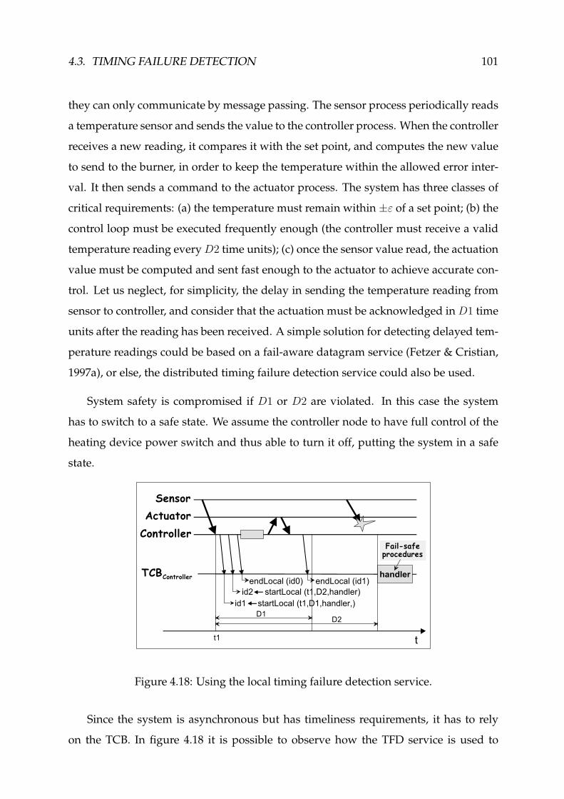
4.3. TIMING FAILURE DETECTION 101
they can only communicate by message passing. The sensor process periodically reads
a temperature sensor and sends the value to the controller process. When the controller
receives a new reading, it compares it with the set point, and computes the new value
to send to the burner, in order to keep the temperature within the allowed error inter-
val. It then sends a command to the actuator process. The system has three classes of
critical requirements: (a) the temperature must remain within ±ε of a set point; (b) the
control loop must be executed frequently enough (the controller must receive a valid
temperature reading every D2 time units); (c) once the sensor value read, the actuation
value must be computed and sent fast enough to the actuator to achieve accurate con-
trol. Let us neglect, for simplicity, the delay in sending the temperature reading from
sensor to controller, and consider that the actuation must be acknowledged in D1 time
units after the reading has been received. A simple solution for detecting delayed tem-
perature readings could be based on a fail-aware datagram service (Fetzer & Cristian,
1997a), or else, the distributed timing failure detection service could also be used.
System safety is compromised if D1 or D2 are violated. In this case the system
has to switch to a safe state. We assume the controller node to have full control of the
heating device power switch and thus able to turn it off, putting the system in a safe
state.
Controller
SensorActuator
D1D2
TCBController
id1 startLocal (t1,D1,handler,)id2 startLocal (t1,D2,handler)
endLocal (id0)
t1 t
endLocal (id1)handler
Fail-safeprocedures
Figure 4.18: Using the local timing failure detection service.
Since the system is asynchronous but has timeliness requirements, it has to rely
on the TCB. In figure 4.18 it is possible to observe how the TFD service is used to

102 CHAPTER 4. DESIGNING TCB SERVICES
detect local timing failures. The controller receives a new temperature reading at in-
stant t1 (measured by the TCB). From this moment on the bounds D1 and D2 must be
checked, and so it is necessary to invoke the startLocal function twice. Note the call
endLocal (id0) after the other two: the call disables detection for the previous period
(D2 specification, not shown), since a new message arrived. The controller then sends
a command to the actuator and, when it receives the acknowledgment, endLocal is
called again, this time to terminate the execution of id2. Normally, neither D1 nor D2
expire. If the computation takes so long that D1 expires, or if a message is not received
from the sensor before D2 expires (as depicted), the handler is immediately executed
by the TCB. The handler function passed as argument can be a very simple function
that is executed by the TCB, issuing a command to the actuator that turns off the heat-
ing device.
A distributed execution requires at least one message to be sent between two pro-
cesses. Thus, the action to be observed for timing failure detection, in addition to local
actions, is message delivery. Since a delivery delay is bounded by a send and a receive
event, the TFD service just has to intercept message transmissions. The described inter-
face provides not only the required functionality but also allows message interceptions
to be done in a very simple and intuitive manner. In the following functions we only
present the TFD service-specific parameters (we omit normal parameters such as ad-
dresses, etc.).
id ← send (send ts, t spec, handler)
id,deliv ts ← receive ()
The meaning of the send function parameters is similar to the ones of the
startLocal function. We assume it is possible to multicast a message to a set of
destination processes using this send function. The receive function blocks the ap-
plication until a message is received. On return, the function provides a message id
and a timestamp for the delivery event. The information relative to timing failures is
queried by means of another function:
id,dur 1,faulty 1 · · · dur n,faulty n ← waitInfo

4.3. TIMING FAILURE DETECTION 103
The function waitInfo blocks the calling process until there is information avail-
able relative to timing failures of some message (identified, on return, by id ). Typically,
an application should be constructed to have a thread for message reception and an-
other to process timing failure information. waitInfo returns the delivery delay and
the failure result for each receiver process of message id .
This service can be useful for many applications. For instance, in the example of
figure 4.17, we may now extend the response time control (D1) back to the sensor read-
ing moment, to enforce the freshness of sensor readings. In order to achieve that, the
sensor message would be sent using this interface, by specifying some maximum de-
livery delay. Upon message reception the waitInfo function could be used to detect
a timing failure. Several other examples of applications where the timing failure detec-
tion could be useful can be found in the literature (Almeida & Verıssimo, 1996; Fetzer
& Cristian, 1997b; Essame et al., 1999).
So far we have not mentioned how the handler is used in the context of the dis-
tributed timing failure detection service. The interface described above allows for an
handler to be executed at the sender process, as if it was the responsible for the tim-
ing failure. In fact, it is true that with the interface proposed above, which considers
a distributed timed action to strictly correspond to a message transmission, the vari-
ability of the message delay is mostly dictated by the time the sender takes to send the
message. So it makes sense to execute the handler at the sender.
However, in some application contexts it would be better to consider a more gen-
eral definition of distributed timed actions, in which both the start and the termination
events are dictated by the application (until now, only the start event was specified
by the application). Therefore, we now introduce three additional interface functions
for distributed timing failure detection, assuming that the termination event is only
triggered by the receiver when it considers that the action has been terminated.
id ← sendWRemoteTFD (start ts, t spec, handler)
id ← receiveWRemoteTFD ()
end ts ← endDistAction (id)

104 CHAPTER 4. DESIGNING TCB SERVICES
sendWRemoteTFDis used just like the send function, to send a message to a set of
destination processes, starting a duration measurement using timestamp start ts
and using t spec as a bound to be observed by the timing failure detection ser-
vice. The difference between the two functions is that with this new one the specified
handler will be executed in the remote site, instead of the sender site.
Now that a distributed action does not simply terminates upon message recep-
tion, the receive function must be a different one since no termination event timestamp
can be returned to the application. This is why the function receiveWRemoteTFD is
provided. On the other hand, it is necessary to provide the means for the receiver pro-
cess to signal the termination of the distributed timed actions, which it can do using
endDistAction . For the TCB to know which is the action that is being terminated,
the id that was obtained when the message (part of the timed action chain) was re-
ceived has to be supplied when issuing endDistAction . On return, the timestamp
that marks the termination event is provided to the application.
In order to implement these new functions, the information that has to be ex-
changed among TFD instances must now be different, for instance to include the spec-
ification of the handler that must be executed in the remote site. In Section 5.6.3, when
showing how the TCB can be useful to achieve timing fault tolerance using replication,
we will see how these interface functions can be used in a concrete situation.
4.4 The complete TCB interface
Table 4.1 summarizes the API for the TCB services. It must be noted, however, that
this API should not be understood as strictly rigid. As the reader will notice in subse-
quent parts of this text, we will introduce slightly modified versions of this interface,
namely when some parameters omitted here become relevant or to modify the level of
abstraction provided by the API (which depends on how the interposition principle—
see Section 3.2— is applied).

4.5. SUMMARY 105
Duration measurementtimestamp ← getTimestamp ()id ← startMeasurement (start ts)end ts,duration ← stopMeasurement (id)
Timely executionend ts ← exec (start ts, delay, t exec max, func)
Local timing failure detectionid ← startLocal (start ts, t spec, handler)end ts,duration,faulty ← endLocal(id)
Distributed timing failure detectionid ← send (send ts, t spec, handler)id,deliv ts ← receive ()id ← sendWRemoteTFD (start ts, t spec, handler)id ← receiveWRemoteTFD ()end ts ← endDistAction (id)id,dur 1,faulty 1 · · · dur n,faulty n ← waitInfo()
Table 4.1: Summary of the API.
4.5 Summary
This chapter was devoted to the discussion of TCB services. Two protocols have
been presented, for distributed duration measurement and for distributed timing fail-
ure detection, which can be used in the construction of the services. In addition, the
TCB interface was described and several examples were presented to illustrate the cor-
rect way to program applications using most of the interface functions. Given that
the next chapter deals with dependable programming using the TCB, some additional
examples will be provided there.
Notes
The improved round-trip protocol presented in this section was designed
in collaboration with Pedro Martins and Luıs Rodrigues. It was presented
in “Measuring Distributed Durations with Stable Errors”, Casimiro, Mar-
tins, Verıssimo and Rodrigues, Proceedings of the “22nd IEEE Real-Time

106 CHAPTER 4. DESIGNING TCB SERVICES
Systems Symposium”, London, UK, December 2001.
The protocols for the timing failure detection service were presented in
“Timing Failure Detection with a Timely Computing Base”, Casimiro and
Verıssimo, Proceedings of the “European Research Seminar on Advances in
Distributed Systems”, Madeira, Portugal, April 1999.
The basic version of the TCB interface was presented in “The Timely Com-
puting Base: Timely Actions in the Presence of Uncertain Timeliness”,
Verıssimo, Casimiro and Fetzer, Proceedings of the “International Confer-
ence on Dependable Systems and Networks”, New York, USA, June 2000.
However, some extensions and refinements have been introduced in more
recent work.

5Dependable programming
with the TCB
The availability of a distributed system model and a programming model specifi-
cally concerned with the design of applications with timeliness requirements in envi-
ronments of uncertain synchrony is fundamental to address many of the existing and
emerging applications. However, in order to develop even better applications, they
should be constructed taking dependability concerns into account.
This chapter provides a comprehensive discussion of several issues related with
the construction of dependable applications using the TCB. To start with, one of the
impairments to dependability – failures – is studied in Section 5.1. If the objective is to
program dependable applications, the first thing that must be done is to clearly under-
stand what are the possible effects of timing failures on the correctness of applications
(note that the mechanisms to handle other kinds of failures are much better under-
stood). It will then be possible to establish the objectives that a dependable design
should follow to avoid those effects in spite of the occurrence of timing failures.
How to achieve these objectives is a crucial problem that is addressed in Section 5.2.
There, it is shown that a few fundamental applications classes exist, and that not all
these classes can benefit from the TCB in the same manner in order to achieve coverage
stability or no-contamination, the generic properties that ensure a dependable design.
The remaining sections discuss timing fault tolerance issues, defining a taxonomy
for timing fault tolerance and proposing new paradigms to help the construction of
dependable applications using the TCB services. In concrete, the notion of dependable
adaptation is introduced and a paradigm for timing fault tolerance using a replicated
state machine is described. The DCCS example is revisited in the end of the chapter.
107

108 CHAPTER 5. DEPENDABLE PROGRAMMING WITH THE TCB
5.1 Effects of timing failures
How can the TCB help design dependable and timely applications? A constructive
approach consists in analyzing why systems fail in the presence of uncertain timeli-
ness, and deriving sufficient conditions to solve the problems encountered, based on
the behavior of applications and on the properties of the TCB.
As we explained earlier, we use ’application’ to denote a computation in general,
defined by a set of safety and timeliness properties PA. We also remind the reader that
we consider a model where components only do late timing failures. In the absence
of timing failures, the system executes correctly. When timing failures occur, there are
essentially three kinds of problems, that we define and discuss below:
• unexpected delay
• contamination
• decreased coverage
The immediate effect of timing failures may be twofold: unexpected delay and/or
incorrectness by contamination. We define unexpected delay as the violation of a time-
liness property. That can sometimes be accepted, if applications are prepared to work
correctly under increased delay expectations, or it can be masked by using timing fault
tolerance (as we discuss in Section 5.6.2). However, there can also be contamination,
that we define as the incorrect behavior resulting from the violation of safety proper-
ties on account of the occurrence of timing failures. This effect has not been well un-
derstood, and haunts many designs, even those supposedly asynchronous, but where
aggressive timeouts and failure detection are embedded in the protocols (Chandra &
Toueg, 1996; Chandra et al., 1996a). In fact, problems such as described in (Anceaume
et al., 1995; Chandra et al., 1996a) assume a simple dimension, when explained un-
der the light of timing failures. These designs fail because: (a) although time-free by
specification, they rely on time, often in the form of timeouts; (b) they are thus prone
to timing failures (e.g., when timeouts are too short); (c) however, proper measures
are not taken to counter timing failures (because they were not supposed to exist in
the first place!); (d) in consequence, error confinement is not ensured, and sometimes

5.1. EFFECTS OF TIMING FAILURES 109
timing failures contaminate safety properties1. A particular form of the contamina-
tion problem was described in the context of ordered broadcast protocols in (Gopal &
Toueg, 1991).
In this thesis, we give a generic definition of the problem, for a system with omis-
sive failures. If the system has the capacity of timely detecting timeliness violations, then
contamination can be avoided with adequate algorithm structure. To provide an in-
tuition on this, suppose that the system does not make progress without having an
assurance that a previous set of steps were timely. Now observe that “timely” means
that the detection latency is bounded. In consequence, if it waits more than the detec-
tion latency, absence of failure indication means “no failure”, and thus it can proceed.
If an indication does come, then it can be processed before the failure contaminates
the system, since the computation has not proceeded. The only consequence of this
mechanism is an extra wait of the order of the detection delay (which is bounded, ac-
cording to Property TCB4). A sufficient condition for absence of contamination is thus
to confine the effect of timing failures to the violation of timeliness properties alone,
specified by the following property:
No-Contamination: Given a history H(TP) derived from property P ∈ PA, H
has no-contamination iff for any timing failure in any execution X ∈ H, no safety
property in PA is violated.
The reader will note that in the model of Chandra (Chandra & Toueg, 1996), the
agreement algorithms have no-contamination, since their design is completely time-
free, and all possible problems deriving from timing failures (such as “wrong suspi-
cions”) are encapsulated in the failure detector. Chandra then bases the reliability of
his system on the possibility of implementing a given failure detector, but he does not
discuss this implementation. In contrast, we define an architectural framework where
aside of the payload part containing the algorithms or applications, a placeholder ex-
ists for the viable implementation of special services such as failure detection— the
control part. One important advantage is generality of the programming model, by
1As a matter of fact they may also contaminate liveness properties, by preventing progress. However,we are mostly interested in safety properties.

110 CHAPTER 5. DEPENDABLE PROGRAMMING WITH THE TCB
letting the payload system have any degree of synchrony. That is, we devise a sin-
gle framework for correct execution of synchronous and asynchronous applications,
of several grades that have been represented by partial models such as asynchronous
with failure detectors, timed asynchronous, or quasi-synchronous. Or, in other words,
from non real-time, through soft, mission-critical, to hard real-time.
Let us talk now about decreased coverage as the other effect of timing failures.
Whenever we design a system under the assumption of the absence (i.e., prevention)
of timing failures, we have in mind a certain coverage, which is the degree of cor-
respondence between system timeliness assumptions and what the environment can
guarantee. We define assumed coverage PP of a property P as the assumed probabil-
ity of the property holding over an interval of reference. This coverage is necessarily
very high for timeliness properties of hard real-time systems, and may be somewhat
relaxed for other realistic real-time systems, like mission-critical or soft real-time. Now,
in a system with uncertain timeliness, the above-mentioned correspondence is not con-
stant, it varies during system life. If the environment conditions start degrading to
states worse than assumed, the coverage incrementally decreases, and thus the prob-
ability of timing failure increases. If on the contrary, coverage is better than assumed,
we are not taking full advantage from what the environment gives. Both situations are
undesirable, and this is a generic problem for any class of system relying on the as-
sumption/coverage binomial (Powell, 1992): if coverage of failure mode assumptions
does not stay stable, a fault-tolerant design based on those assumptions will be im-
paired. A sufficient condition for that not to happen consists in ensuring that coverage
stays close to the assumed value, over an interval of mission. Formally, we specify this
condition by the following property:
Coverage Stability: Given a historyH(TP) derived from property P ∈ PA, with
assumed coverage PP , H has coverage stability iff the set of executions contained
in H is timely with a probability pH, such that |pH − PP | ≤ pdev, for pdev known
and bounded.
The Coverage Stability property can be explained very easily. If we adapt our time-
liness requirements say, by relaxing them when the environment is giving poorer ser-

5.2. MAKING APPLICATIONS DEPENDABLE 111
vice quality, and tightening them when the opposite happens, we maintain the actual
coverage (pH) around a desirably small interval of confidence of the assumed cover-
age (PP). The interval of confidence pdev is the measure in which coverage stability is
ensured. Note that even if long term coverage stability is ensured, instantaneously the
system can still have timing failures, as we have previously discussed.
The next step is to prove that the TCB helps applications to secure coverage stability
and no-contamination, despite the uncertainty of the environment. In all that follows,
we consider the availability of the TCB services. Proofs of the lemmata and theorems
given are shown in appendix.
5.2 Making applications dependable
Now that we have analyzed the effect of timing failures, we know what are the
properties that should be secured in order to make applications dependable. However,
not all applications can enjoy these properties. This section is concerned with showing
that some application classes can indeed enjoy these properties, with the help of the
TCB. We first concentrate on the coverage stability property and then we describe how
to avoid contamination.
5.2.1 Enforcing Coverage Stability with the TCB
We start with a definition of coverage stability for an application. Recall the defini-
tions made in Section 3.1, of histories and the ’derived-from’ relation.
Definition 1 An application A has coverage stability iff all histories derived from properties
of A have coverage stability:
∀P ∈ PA, ∀H s.t.H−→d P : H has coverage stability
Not all applications can benefit from the Coverage Stability property. Let us define
a useful class that can indeed benefit.

112 CHAPTER 5. DEPENDABLE PROGRAMMING WITH THE TCB
Definition 2 Time-Elastic Class (T ε) - Given an application A, represented by a set of prop-
erties PA, A belongs to the time-elastic class T ε, iff none of the duration bounds derived from
any property P of A are invariant2:
A ∈ T ε∆= ∀P ∈ PA, ∀T s.t. T −→d P : T is not an invariant
In practical terms, T ε applications are those whose bounds can be increased or
decreased dynamically, such as QoS-driven applications. We now show the conditions
under which a T ε application achieves coverage stability. We start by establishing
the capability of the TCB to make histograms of the distribution of durations (service
TCB2) and thus gathering evidence about actual coverage.
Observe an example distribution (probability density function or pdf ) of a dura-
tion T , depicted in Figure 5.1. If we focus on the pair (Tf , Pf ) over curve A, Pf is the
probability of finding executions lasting Tf . Consequently, if Tf were an assumed up-
per bound, the shaded part of the distribution would contain executions with timing
failures. The coverage of this assumption is thus given by the area of the distribution
outside the shaded part. On the other hand, as we state in Lemma 1 below, the pdf will
obviously have a certain error.
Lemma 1 Given a history H(T ) containing a finite initial number of executions n0, the TCB
can compute the probability density function pdf of the duration T bounded by T and there
exists a pdev0 known and bounded, such that for any P = pdf(T ), and p the actual probability
of T , it is |p− P | ≤ pdev0
The pdf construction will be subjected to the TCB duration measurement error
(TDURmin), and to extrapolation errors, given by the measure in which the n0 samples
are representative of the distribution.
On the other hand, in systems of uncertain timeliness, the pdf of a duration varies
with time. For example, consider that curve A as depicted in Figure 5.1 represents the
behavior of duration T during some initial period, and that from then on, the system’s
load increases such that executions become slower. Normally, if a sufficiently large
2Invariant is taken in the sense of not being able to change during the application execution.

5.2. MAKING APPLICATIONS DEPENDABLE 113
AB
TB
Pf
P(T)
T
PB
Tf
Figure 5.1: Example variation of distribution pdf(T ) with a changing environment
interval of observation is considered, so as to damp short-term instability, what can
be observed is a shift of the baseline pdf , as depicted in Figure 5.1 by curve B. How-
ever, more complex behaviors may arise. For the results of this thesis, it is enough to
establish that the long-term pdf error pdev remains bounded, as we state in Lemma 2
below.
Lemma 2 Given pdfi−1(T ), of duration T in H(T ), and given any immediately subsequent
n executions, the TCB can compute pdfi(T ) and there exists a pdev known and bounded, such
that for any P = pdfi(T ), and p the actual probability of T , it is |p− P | ≤ pdev
What Lemma 2 proposes is that a new set of samples composed of part of the old
history, plus the new n executions, is representative (under the same error constraints
discussed for Lemma 1) of the actual current distribution. Essentially, the lemma states
that given n new samples, by using the adequate balance with a part of the previous
distribution, the error pdev remains bounded.
However, one also wishes to keep the error pdev small in order to predict the prob-
ability of any T accurately, even with periods of timeliness instability. We are cur-
rently studying efficient functions to keep pdev small, in the presence of large devia-
tions (Wold, 1965). The reader may wonder that it is impossible to predict the future,
and thus using the pdf to assert timing variables for the future operation does not make
sense. Note however: (a) some systems (with fixed assumptions) in fact predict the fu-
ture off-line (e.g., by testing and assuming that the future will be like the present); (b)
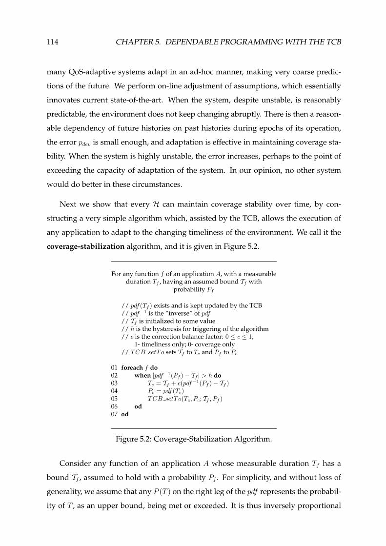
114 CHAPTER 5. DEPENDABLE PROGRAMMING WITH THE TCB
many QoS-adaptive systems adapt in an ad-hoc manner, making very coarse predic-
tions of the future. We perform on-line adjustment of assumptions, which essentially
innovates current state-of-the-art. When the system, despite unstable, is reasonably
predictable, the environment does not keep changing abruptly. There is then a reason-
able dependency of future histories on past histories during epochs of its operation,
the error pdev is small enough, and adaptation is effective in maintaining coverage sta-
bility. When the system is highly unstable, the error increases, perhaps to the point of
exceeding the capacity of adaptation of the system. In our opinion, no other system
would do better in these circumstances.
Next we show that every H can maintain coverage stability over time, by con-
structing a very simple algorithm which, assisted by the TCB, allows the execution of
any application to adapt to the changing timeliness of the environment. We call it the
coverage-stabilization algorithm, and it is given in Figure 5.2.
For any function f of an application A, with a measurableduration Tf , having an assumed bound Tf with
probability Pf
// pdf(Tf ) exists and is kept updated by the TCB// pdf−1 is the ”inverse” of pdf// Tf is initialized to some value// h is the hysteresis for triggering of the algorithm// c is the correction balance factor: 0 ≤ c ≤ 1,
1- timeliness only; 0- coverage only// TCB setTo sets Tf to Tc and Pf to Pc
01 foreach f do02 when |pdf−1(Pf )− Tf | > h do03 Tc = Tf + c(pdf−1(Pf )− Tf )04 Pc = pdf(Tc)05 TCB setTo(Tc, Pc; Tf , Pf )06 od07 od
Figure 5.2: Coverage-Stabilization Algorithm.
Consider any function of an application A whose measurable duration Tf has a
bound Tf , assumed to hold with a probability Pf . For simplicity, and without loss of
generality, we assume that any P (T ) on the right leg of the pdf represents the probabil-
ity of T , as an upper bound, being met or exceeded. It is thus inversely proportional

5.2. MAKING APPLICATIONS DEPENDABLE 115
to the coverage of T , and can be used to represent it. Whenever the application exe-
cutes the function, this is made known to the TCB in the form of a timed action with
the adequate parameters. Typically, this action can be the sending of a message (which
generates a remote event) or the execution of a local function, and its latest termina-
tion instant te is determined by the start instant and the bound Tf . The TCB follows
the execution of these actions, and in consequence the coverage-stabilization algorithm
assumes that the TCB has created pdf(Tf ) and keeps it updated. We also assume that,
given pdf , it is then easy to extract an approximation of value T for any P . We denote
this operation by pdf−1. In consequence, pdf−1(Pf ) is the observed duration that holds
with the desired probability Pf (it may have deviated from the assumed Tf ).
Consider that curve A in Figure 5.1 represents the initial steady-state operational
environment for Tf : if P = Pf , then T ' Tf . Whenever the TCB detects a signifi-
cant variation in the environment (line 2), that is, when pdf−1(Pf ) exceeds an interval
h around Tf , the algorithm is triggered. Parameter h introduces hysteresis in the algo-
rithm operation, to prevent it from oscillating back and forth. The second parameter
of the algorithm is c, the correction balance factor. c assumes any value between zero
and one, and allows a combined correction of both timeliness and coverage.
Timeliness is adjusted in the following form: Tf is a variable of the application
code from which all parameters needed to substantiate the assumption in runtime (e.g.,
timeouts, multimedia protocol timing parameters, etc.) are derived. Tf is set to some
initial value. The algorithm computes a new value Tc and automatically updates Tf ,
influencing all parameters.
As for coverage, once having determined the new timeliness value, the algorithm
computes Pc = pdf(Tc). The reader should note that once the principle understood,
nothing prevents us from implementing fancier schemes: a) replacing this function by
one that computes the coverage value more accurately, given the area of the unshaded
part; b) allowing to choose between computing timeliness first and then coverage or
vice-versa.
These adjustments are computed in lines 3 and 4. Assume timeliness degrades:
if c = 1, only timeliness is corrected, in order to preserve coverage at the originally

116 CHAPTER 5. DEPENDABLE PROGRAMMING WITH THE TCB
desired value; if c = 0, the timeliness bound is preserved, and coverage expectations
are decreased. We represent the update (line 5) by a function TCB setTo(), whereby
the TCB automatically updates variables which are accessible to the application. The
semantics of TCB setTo() in our example is as simple as “setting Tf = Tc and Pf = Pc”.
However, a practical algorithm may have more elaborate semantics tuned to specific
QoS applications.
To understand the mechanism, let us look again at Figure 5.1: the environment
got slower, and there was a shift of pdf to the right (curve B). From the graphic, the
value for the bound that still complies with P = Pf is now TB. If TB is substituted
in Tf (i.e., for c = 1, Tc = TB), the application maintains the degree of coverage but
admits to get slower. Alternatively, maintaining the original t = Tf timeliness bound
implies that the application wishes to retain the same speed on average, but accepts
a decreased coverage value, since the shaded area delimited by PB is larger (i.e., for
c = 0, Pc = PB = pdf(Tf )). For intermediate values of c the timeliness and probability
values lie between these extremes.
Note that these remarks are also true when the environment performs better (faster
and/or more reliable): the variables should get back to their original values as soon as
possible, in order to take advantage from an improved QoS situation. However, they
are only changed again when the measured bound deviates from Tf more than h, the
hysteresis of the algorithm.
The discussion above allows us to introduce the first theorem about applications
based on a TCB, whose proof is in the appendix.
Theorem 3 An application A ∈ T ε using a TCB and the coverage-stabilization algorithm has
coverage stability
5.2.2 Avoiding Contamination with the TCB
We start with a definition of no-contamination for an application.
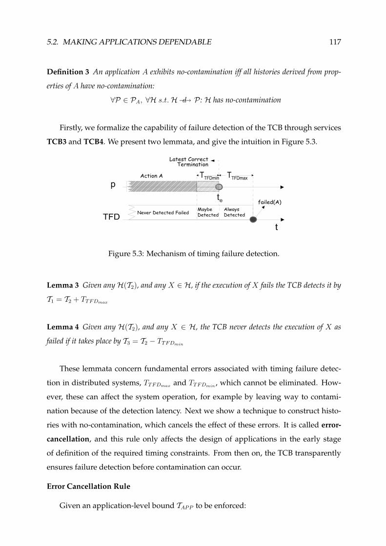
5.2. MAKING APPLICATIONS DEPENDABLE 117
Definition 3 An application A exhibits no-contamination iff all histories derived from prop-
erties of A have no-contamination:
∀P ∈ PA, ∀H s.t.H−→d P : H has no-contamination
Firstly, we formalize the capability of failure detection of the TCB through services
TCB3 and TCB4. We present two lemmata, and give the intuition in Figure 5.3.
Figure 5.3: Mechanism of timing failure detection.
Lemma 3 Given anyH(T2), and any X ∈ H, if the execution of X fails the TCB detects it by
T1 = T2 + TTFDmax
Lemma 4 Given any H(T2), and any X ∈ H, the TCB never detects the execution of X as
failed if it takes place by T3 = T2 − TTFDmin
These lemmata concern fundamental errors associated with timing failure detec-
tion in distributed systems, TTFDmax and TTFDmin, which cannot be eliminated. How-
ever, these can affect the system operation, for example by leaving way to contami-
nation because of the detection latency. Next we show a technique to construct histo-
ries with no-contamination, which cancels the effect of these errors. It is called error-
cancellation, and this rule only affects the design of applications in the early stage
of definition of the required timing constraints. From then on, the TCB transparently
ensures failure detection before contamination can occur.
Error Cancellation Rule
Given an application-level bound TAPP to be enforced:

118 CHAPTER 5. DEPENDABLE PROGRAMMING WITH THE TCB
• define the application logic (e.g., timeliness properties, timeouts) in terms of
bound TAPP
• design the environment in order to secure at least TENV = TAPP − TTFDmax −
TTFDmin
• set the TCB failure detection logic to trigger at TTFD = TAPP − TTFDmax
The error cancellation rule yields interesting results. For a real execution delay
bound of TENV , the application must work with a safety margin of at least TTFDmax +
TTFDmin, because of the basic delay and inaccuracy of failure detection. However, for
the adjusted bound TAPP = TENV +TTFDmax+TTFDmin, it is possible to simulate virtually
instantaneous and accurate detection:
• any timing failure is detected (by the TCB) by TAPP
• any timely execution is never detected as failed
In other words, the error cancellation rule proposes to use different values for each
of the three above-mentioned aspects of building an application: given TENV , the real
bound met by the support environment, we use TTFD = TENV + TTFDminas the failure
detection threshold, and TAPP = TTFD+TTFDmax as the bound visible to the application.
Now we proceed with our treatment of contamination. Not all applications can
benefit from the No-Contamination property. Intuitively, the least effective class that
can indeed benefit is the fail-safe class, since it stops upon the first detected timing
failure.
Definition 4 Fail-Safe Class (Fσ) - Given an application A, represented by a set of prop-
erties PA, A belongs to the fail-safe class Fσ, iff there is a state sFS to which A can transit
permanently, from any state si, at any time tFS , such that for any safety property P of A, if P
was true in time interval [..., tFS[, it remains true for [tFS, ...[:
A ∈ Fσ∆= ∃sFS∀si∀tFS :
(sitFS→ sFS) ∧ ∀(P ∈ PS ∩ PA)((∀t < tFS, t |= P)⇒ (∀t ≥ tFS, t |= P))

5.2. MAKING APPLICATIONS DEPENDABLE 119
In practical terms, Fσ applications are those that can switch at any moment to a
fail-safe state and remain there permanently, such that the system’s safety properties
remain valid. Note that whilst this seems to be a given in systems with hardware fail-
safe switches, watchdogs, etc., it is not so in generic distributed systems with uncertain
timeliness. Systems running under models that do not have the capabilities expressed
by Property TCB1, of executing functions with guaranteed delays in any situation (in
practice all but fully synchronous systems), cannot be guaranteed to be fail-safe. In
our model, this ability, for any asynchrony of the payload system, is secured by running
fail-safe shutdown routines inside the TCB. Plus, these routines can be coordinated and
run locally in several hosts of the system. We now have the second theorem about
applications based on a TCB.
Theorem 4 An application A ∈ Fσ using a TCB has no-contamination
The discussion above allows us to capture the intuition behind this claim: by using
the error cancellation rule, failures are not wrongly detected, and any failure is detected
by T ; since prior to T there was no evidence of failure, if we switch the system to the
fail-safe state immediately a failure is detected (i.e., tFS), the corresponding history
H(T ) has no-contamination.
It is not interesting to halt an application upon the first timing failure, if better can
be done. However, we know that not all applications can enjoy the No-Contamination
property after timing failures occurring. We define a class that can.
Definition 5 Time-Safe Class (T σ) - Given an application A, represented by a set of proper-
ties PA, A belongs to the time-safe class T σ, iff no historiesH(TP) are derived from any safety
property in PA
A ∈ T σ∆= ∀P ∈ PA, ∀H s.t.H−→d P : ¬(P ∈ PS)
In practical terms, T σ applications are those where: timeliness properties are
clearly separated from logical safety ones; the code implementing safety properties
does not depend on time (e.g. timeouts). These applications have a neat construction

120 CHAPTER 5. DEPENDABLE PROGRAMMING WITH THE TCB
where timing failures are confined to just one of the three failure symptoms we stud-
ied in Section 5.1: unexpected delay. In consequence, one can implement mechanisms
that address timing fault tolerance, without being concerned with the logical integrity
of the application. We claim that a T σ application achieves no-contamination, in a
theorem expressing the third and final facet of the timely computing base model.
Theorem 5 An application A ∈ T σ using a TCB has no-contamination
5.3 A taxonomy for timing fault tolerance
Timing failures, in a fault-tolerance sense, can be handled in one of the following
ways: masking; detection and/or recovery. A generic approach to timing fault tolerance,
that is, one that can use any or all of the methods above, requires the following basic
attributes:
• timeliness- to act upon failures within a bounded delay;
• completeness- to ensure that failure detection is seen by all participants;
• accuracy- not to detect failures wrongly;
• coverage- to ensure that assumptions hold during the lifetime of the system (e.g.
number of failures and magnitude of delays);
• confinement- to ensure that timing failures do not propagate their effect.
These attributes are mostly ensured by the TCB and its services. The last two are
secured indirectly, by the Coverage Stability and No-Contamination properties. Fur-
thermore, our model is able to distinguish between several mechanisms of timing fail-
ure:
• decreased coverage;
• unexpected delay;
• contamination.
In consequence, one should be able to program real-time applications which have
several degrees of dependability, despite the occurrence of timing failures: by detecting

5.4. FAIL-SAFE OPERATION 121
timing failures and still being able to recover by reconfiguration (e.g. by postponing
a decision, by increasing the deadline, etc.); by detecting irrecoverable timing failures
and doing a fail-safe shutdown; by masking independent timing failures with active
replicas.
The TCB provides a framework for addressing all of these techniques, for any de-
gree of synchronism of the payload system. We consider increasingly effective fault
tolerance mechanisms, requiring combinations of the following attributes:
• timing failure detection (TFD)
• fail-safety (Fσ)
• time-safety (T σ)
• time-elasticity (T ε)
• replication (REP)
TFD comes by default in the TCB. Fail-safety, time-safety, and time-elasticity cor-
respond to application programming styles. Replication introduces a novel approach
to real-time computing, by applying the classical concepts of fault tolerance to timing
faults. As long as the latter are temporary and independent, the application remains
timely, despite timing faults in some replicas.
The next sections will focus on each of the above-mentioned techniques for achiev-
ing different degrees of dependability. Depending on the class of application under
consideration, we explain the methodology for the latter to achieve their (dependabil-
ity) objectives with the help of the TCB.
5.4 Fail-safe operation
By Theorem 4, any class of application with a fail-safe state can be implemented
using a TCB. This is because the TCB has the ability of detecting timing failures in
a timely manner. However, care must be taken with the setting of bounds, to avoid
contamination. It is not enough to detect a failure and shutdown: the timely execution
of these operations is crucial. The methodology should be the following:

122 CHAPTER 5. DEPENDABLE PROGRAMMING WITH THE TCB
• define all important timing parameters so that timing failures can be detected by
the TCB;
• the error-cancellation rule (Section 5.2.2) should be followed, so that failure de-
tection can be done before any harm happens, and if nothing else can be done, at
least the application fails-safe before getting incorrect;
• moreover, since all processes can be informed by the TCB of failure occurrences,
switching to a fail-safe state can be done in a controlled way in the case of dis-
tributed or replicated applications.
Several examples of applications with a fail-safe state can be encountered in the
literature (Lubaszewski & Courtois, 1998; Fetzer & Cristian, 1996c; Fetzer & Cristian,
1997b). In the examples described in (Fetzer & Cristian, 1996c) and (Fetzer & Cristian,
1997b), the authors show how a fail-safe application can be implemented in the timed
asynchronous model. The detection of timing failures is done by using fail aware ser-
vices but the assurance of crucial safety properties also requires communication by
time in the realm of the application. While fail-safety has been ensured in the works
we know of on a case-by-case basis, the novelty of our approach is that instead of giv-
ing an implementation, we define a class (Fσ) of applications. Any implementation of
an application of this class on the TCB can achieve no-contamination in the presence
of timing failures, regardless of other aspects of its semantics. The TCB model also
removes an ambiguity sometimes encountered in previous works: systems with un-
bounded execution time state the capability of immediate (timely) fail-safe shutdown,
an apparent contradiction. Switching to the fail-safe state in a timely manner can be
ensured by the TCB, no matter how asynchronous the payload system.
In the example presented in (Fetzer & Cristian, 1996c), a railway crossing system,
the main safety property is that the gates must be down whenever a train is in the
railway crossing. However, to achieve liveness it is necessary to open the gates when
no train is in the crossing. During normal operation the controllers send “Gate up” or
“Gate down” commands to the gate units based on the information they periodically
receive, through a network, from sensor units. If a gate unit does not receive a valid
command (one not affected by timing failures) for a specific amount of time, it switches
to its safe mode. Note that for this switching action to take place in a timely manner,

5.5. RECONFIGURATION AND ADAPTATION 123
the gate units must be synchronous components.
With a TCB, the controllers would use the TFD service when sending their com-
mands (more specifically, the sendWRemoteTFDfunction), so that delayed commands
would force an handler to be executed in the gate units in a timely manner (real-time
is only needed for the handler).
The traffic signaling example (Fetzer & Cristian, 1997b) requires the switching to
the safe mode to be done in a controlled way, since it is necessary to prevent that
one traffic light flashes red while another shows green. With the TCB the design of a
solution can be made easier due to the timing failure detector properties. In fact, when
a traffic light node switches to the safe state, based on the information provided by the
TCB, all other nodes will know of that decision because they also have access to the
same information. Thus, using the timely execution properties of the TCB, every node
can control, in a timely fashion, when to switch the lights.
As a final example, we mention a fully-automated train control system that
achieves availability using replicated fail-safe components (Essame et al., 1999). The
aspect that is most relevant to us in this example is that the communication subsystem
is based on the timed asynchronous model, which allows the coverage to be higher
since timing failures are assumed in the model. Nevertheless, the system has a real-
time executive to guarantee that some operations are executed on time in order to
preserve the safety of the system. To some extent, this real-time part of the system can
be viewed as a TCB that executes the timely shut-down, whilst the payload part of the
system is, in this case, a timed asynchronous environment.
5.5 Reconfiguration and adaptation
A more effective approach, other than simply halting the system, is trying to keep
the application running. Again, this can be done on a case-by-case basis, or by defining
classes of applications with given attributes, namely time-elasticity or time-safety.
It is very interesting to verify that a lot of work has been done recently in study-

124 CHAPTER 5. DEPENDABLE PROGRAMMING WITH THE TCB
ing and proposing ways of dealing with QoS adaptation (Abdelzaher & Shin, 1998;
Almeida & Verıssimo, 1996; Cosquer et al., 1995; Bagchi et al., 1998; Cukier et al., 1998;
M. Hiltunen & Schlichting, 1999). The point is that many applications are naturally
able to provide services with different QoS and, therefore, if there is any possibility
of dynamically adapting this QoS to the changing environment, then the application
should do that. However, the works we know of do not always follow a metrics that
relates the QoS adaptation to the dependability issue: coverage stability. Others do es-
tablish thresholds for failure detection, but they cannot guarantee the precision of this
detection, due to the lack of synchrony of the system.
By Theorem 3, applications of the time-elastic class running under the TCB model
provide a means to achieve QoS adaptation while maintaining coverage stability. The
methodology was laid down in Section 5.2.1:
• defining all important timing variables;
• building a pdf for each of those variables with the support of the TCB;
• applying the timeliness-tuning algorithm (Fig. 5.2) to relax or tighten the bounds
dynamically.
Having this property means that it is possible to maintain the application running
at a stable reliability level, despite environment changes to states worse than expected.
This has a cost in the quality of the service the application can give. However, for many
applications it is much better to keep running in a degraded mode (or with a lower
QoS) than stopping, or worse, start having unexpected failures, as per the assumed
coverage. Coverage stability is maintained in both directions: it also means that when
the environment recovers, the application quickly comes back to the initial QoS.
The possibility of achieving coverage stability through adaptation does not prevent
the occurrence of sporadic timing failures. Therefore, we still need to address the effect
of an individual timing failure. Again, there is room for ad-hoc solutions to this prob-
lem but, as shown by Theorem 5, an application possessing the time-safety property is
guaranteed to be free from contamination when timing failures occur, regardless of the
way it is implemented. This means that it is possible to apply the methodology that
was laid down in Section 5.2.2, which is simply based on:
5.5. RECONFIGURATION AND ADAPTATION 125
• specifying applications such that safety and timeliness specifications are neatly
separated;
• having all applications be implemented in a modular fashion, such that the algo-
rithms related with the implementation of safety properties are time-free, that is,
they do not generate timed actions;
• having the implementation of timeliness properties be assisted by the TCB ser-
vices (eager and deferred execution, duration measurement and obviously, tim-
ing failure detection) when necessary;
If the application cannot be constructed in a time-safe way, then it may not have
the no-contamination property, in which case nothing can be done when failures occur
(except halting the application if it has a safe mode). This problem would require more
elaborate application architectures, such as replication, to allow failure masking (see
Section 5.6).
Nevertheless, many applications of the time-elastic class are also time-safe, thus
remaining correct despite the occurrence of occasional timing failures, or fail-safe, thus
able to switch to a safe state after a failure. In the latter case it may seem counter-
intuitive to use adaptation techniques if the application has to do fail-safe switching
(possibly stopping) to cope with isolated timing failures. However, the fact is that
both strategies can be combined in a useful way: When the application recovers from
the timing failure it may adapt the relevant timing variables in order to minimize the
probability of timing failures.
Given the above description of the principles and the basic mechanisms underlying
the construction of dependable time-elastic applications, there are a few aspects that
remain to be discussed in more detail.
First, we believe that it is interesting to understand how is our approach positioned
among the several systems and ways to deal with QoS adaptation. Therefore, we
present a more detailed overview of several QoS approaches in Section 5.5.1. One of the
distinctive aspects of using the TCB for QoS adaptation is that it allows to dependably
adapt applications. While we have already seen, in a general context, how to achieve
dependable adaptation, we still need to to explain how the proposed methodologies

126 CHAPTER 5. DEPENDABLE PROGRAMMING WITH THE TCB
can be used when the focus is on QoS aspects. This is done in Section 5.5.2 where we
first study the particular QoS mechanisms under the TCB framework and then present
a QoS model suitable for the TCB. Finally, the above-mentioned general methodology
to achieve QoS adaptation while maintaining coverage stability deserves to be further
discussed. Section 5.5.3 describes a TCB based QoS coverage service, explaining its
interface and how it is constructed.
5.5.1 QoS based approaches in open environments
The provision of quality of service (QoS) guarantees in open environments, such
as the internet, is currently an active field of research. In fact, although there is a lot
of work dealing with the problem of QoS provision in environments where resources
are known and can be controlled (Vogt et al., 1998; Siqueira & Cahill, 2000; Xu et al.,
2000; Foster et al., 2000), no systematic solution has been proposed for environments
where there is no knowledge about the amount of available resources. Given that the
TCB model characterizes these kind of unpredictable environments in a generic way it
naturally provides an adequate framework to derive solutions for adaptive QoS based
applications.
Most of the works that deal with QoS provision assume that resource reservation
is possible. They address several facets of the problem and propose very diverse solu-
tions. For instance, they propose to use application specified benefit functions as a way
to optimize resource management (Chatterjee et al., 1997), they describe middleware
architectures to deal with heterogeneous environments (Siqueira & Cahill, 2000), they
propose control-based solutions (Li & Nahrstedt, 1999) or they use resource brokers
to manage system resources (Xu et al., 2000). A comprehensive survey about end-to-
end QoS architectures can be found in (Aurrecoechea et al., 1998). The IntServ (Braden
et al., 1994) and DiffServ (Blake et al., 1998) architectures were proposed to specifically
address the problem of handling QoS requirements and differentiated service guaran-
tees in the Internet. An overview of Internet Quality of Service is presented in (Zhao
et al., 2000). Detailed discussions about multimedia applications over the Internet can
be found in (Ferguson & Huston, 1998) and (Wang & Schulzrinne, 1999).

5.5. RECONFIGURATION AND ADAPTATION 127
Unlike the majority of the work dealing with QoS provision, we are concerned
with environments where resource reservation and QoS enforcement may not be pos-
sible. Obviously, not all applications can be implemented on these environments. As
we have already seen, they need to be adaptive or more particularly time-elastic, that is,
they must be able to adapt their timing expectations to the actual conditions of the en-
vironment, possibly sacrificing the quality of other (non time-related) parameters. The
success of an adaptive system has to do essentially with two factors: 1) the monitoring
framework, which dictates the accuracy of the observations that drive adaptation and
2) the adaptation framework, which determines how the adaptation will be realized.
Monitoring of local resources and processes is widely used (Lutfiyya et al., 2001;
Foster et al., 2000), but it does not provide a global view of the environment. Some
works propose adaptation based on network monitoring and on information exchange
among hosts (using specific protocols like RTP (Busse et al., 1996) or estimating de-
lays (Campbell & Coulson, 1996)) but they do not reason in terms of the confidence
about the observations, which is essential for dependable adaptation. In contrast, we
focus on providing a global view of the environment (consistent to all participating
entities) and on ensuring the correctness of that view.
Relatively to adaptation strategies, we mention the work in (Abdelzaher & Shin,
1998), that proposes adaptation among a fixed number of accepted QoS levels, and
the work in (Li & Nahrstedt, 1999), that uses control theory to enhance adaptation
decisions and fuzzy logic to map adaptation values into application-specific control
actions. However, since they have no dependability concerns relative to the adapta-
tion, neither they reason in terms of a generic model of partial synchrony for the dis-
tributed system, we believe our work can complement theirs. These dependability
concerns appear on the AQuA architecture (Cukier et al., 1998), which provides adap-
tation mechanisms to respond to system faults and to maintain certain (dependability
related) QoS levels. Therefore, adaptation in AQuA refers to maintaining a certain
replication degree, based on an imperfect observation of the environment, while we
focus on adapting timing parameters of the application to meet its dependability (tim-
ing fault tolerance) requirements.

128 CHAPTER 5. DEPENDABLE PROGRAMMING WITH THE TCB
5.5.2 Dealing with QoS under the TCB framework
Given the TCB model with its services and interfaces, which we consider the essen-
tial ones to address timeliness issues in unpredictable environments, we now analyze
the implications of using this model to construct QoS architectures.
Quality of Service can have different meanings that depend essentially on the ap-
plication. This is why the definition of a completely generic model for specifying QoS
needs is perhaps an impossible task: it is usually necessary to use mapping mecha-
nisms to translate user level QoS requirements into system level ones. In the present
work we assume that it is possible to define mapping mechanisms, so that QoS require-
ments of different applications can be specified in terms of timing variables, which are
the variables of interest in the TCB model. So to speak, what we need is to define a
TCB QoS model suitable to handle the timeliness and dependability aspects.
5.5.2.1 A QoS model for the TCB
When we think about the specification of QoS requirements in the context of the
TCB model, we intuitively think about timeliness, that is, about the specification of
bounds that must be ensured. Therefore, at first sight we could simply associate QoS
to timeliness and translate all the relevant application QoS requirements into timeliness
requirements. However, we already know that programming dependable time-elastic
applications using the TCB is done by securing the coverage-stability property, which
implies the need to define coverage requirements.
This means that to gain full benefit from the TCB, application QoS requirements
must be specified in terms of 〈bound,coverage〉 pairs. That is, applications must be con-
structed assuming that each time bound holds with a certain coverage. Note that this
way of specifying QoS requirements can also be useful in other contexts, namely when
using the TCB for timing fault tolerance (see Section 5.6.1.3).

5.5. RECONFIGURATION AND ADAPTATION 129
5.5.2.2 Improving QoS mechanisms
Typically, QoS adaptable applications are realized on top of a QoS framework. This
framework is defined by a compound of QoS mechanisms which, altogether, charac-
terize its ability to deal with application QoS requirements. There are three basic cat-
egories of QoS mechanisms: QoS provision, QoS control and QoS management mech-
anisms. If we want to use the TCB as a basic model to serve the design of some end-
to-end QoS architecture, we must investigate the benefits that it might bring for the
implementation of these QoS mechanisms. In particular, and since the TCB model
provides a set of services to applications, we must be able to understand which QoS
mechanisms can be improved by using these TCB services.
Before all, recall that the TCB does not restrict the properties of the payload part of
the system, which allows for any QoS architecture to be implemented in a TCB based
system. In fact, we stress that a TCB is just a small component that, mostly because of
its small size and simplicity, can be constructed with more synchronous properties (or
can be more dependably synchronous) than the rest of the system. Therefore, simply
consider that a TCB can be plugged into any existing system and be used as an oracle
that provides a few basic services. The question is whether these services can be used
to improve the existing QoS mechanisms. Let us first take a look on these mechanisms,
closely following the systematization presented in (Aurrecoechea et al., 1998))
The first category of QoS mechanisms, QoS provision, allows applications to use
low level services, such as communication services, and to specify desired levels of
QoS. QoS provision includes the following: a) QoS mapping – to translate applica-
tion level notation to system level specifications; b) Admission testing – to verify that
there exist enough available resources to admit the requested QoS level; c) End-to-end
reservation – to reserve resources and prevent resource outage during execution.
The second category consists of QoS control mechanisms, which serve to regulate
and control the way in which resources are used and shared by the several flows (traf-
fic or execution flows) during run-time. They include several mechanisms, namely
a) Flow shaping – to regulate usage according to some formal representation (for in-
stance, a statistical one); b) Flow scheduling – to manage the several flows in an in-

130 CHAPTER 5. DEPENDABLE PROGRAMMING WITH THE TCB
tegrated way; c) Flow policing – to verify that the contract is being adhered to by
applications; d) Flow control – to guarantee resource availability, either using open
loop schemes (with advanced resource reservation) or closed loop schemes (with flow
adaptation based on feed-back information); e) Flow synchronization – to account for
precise interactions (e.g. multimedia interactions) of different flows.
Finally, the QoS management category includes the following mechanisms: a) QoS
monitoring – to observe QoS levels achieved by lower layers; b) QoS maintenance –
to perform fine adaptation of resource usage to maintain QoS levels; c) QoS degrada-
tion – to deliver QoS indication to applications when QoS cannot be sustained; d) QoS
availability – to allow applications to specify bounds for QoS parameters; e) QoS scala-
bility – which comprises QoS filtering, to allow the manipulation of (traffic) flows, and
QoS adaptation, to scale flows at the end system in order to respond to fluctuations in
end-to-end QoS.
Now we must recall that TCB services can be used, in a general sense, to help ap-
plications observe their timeliness (using the duration measurement service), execute
short real-time operations (with the timely execution service) or detect timing failures
in a timely fashion and react upon their detection within given time bounds. We must
therefore look for QoS mechanisms that rely directly or indirectly on time, which are
the ones that might be improved using these services.
Of the QoS provision mechanisms, QoS mapping and end-to-end reservation only
perform logical operations and do not need timeliness information to achieve their
goals. Clearly, they are not eligible mechanisms for possible improvements. On the
other hand, admission testing mechanisms need to compare available resources with
requested ones, and so may possibly use the TCB to have the knowledge of available
resources, measured in terms of timeliness. Relatively to QoS control mechanisms, the
one that most clearly can use a TCB, in particular its duration measurement service, is
the closed loop flow control mechanism. The basic idea is to use the information about
distributed durations (relative to end-to-end transmission of data) to derive conclu-
sions about the correct control actions to take. Finally, the QoS management mecha-
nisms that deal with observing the behavior of the environment (or lower level ser-

5.5. RECONFIGURATION AND ADAPTATION 131
vices) can also use information about distributed durations to measure the QoS level
(in terms of timeliness) that is being provided in a given moment.
The fundamental conclusion is that a TCB can essentially be used to improve the
mechanisms that need information about the environment. This is clearly the case of
mechanisms such as the flow control or the QoS monitoring, but can also be the case
of other mechanisms, such as the QoS maintenance, which, by using the output of
a possibly improved monitoring, can also employ finer grain techniques to achieve
better results.
Now that we have seen that a TCB can eventually be useful to construct or im-
prove any QoS mechanism that needs information about the environment, we need
to understand what can be done using the information provided by the TCB. Besides
the obvious possibility of directly using information about timing failures provided by
the TFD service (for instance, to generate alert events in a monitoring module), we are
interested in using the information to adapt the QoS. Therefore, we recall the method-
ology to achieve coverage stability that was introduced in Section 5.2.1.
The methodology consists essentially in constructing a pdf for the relevant timing
variables (based on the timely observation of the environment) and applying an algo-
rithm to adapt the application and to achieve coverage stability. In fact, given that QoS
requirements are specified in terms of 〈bound,coverage〉 pairs, the availability of a pdf
is extremely useful. It allows, for the purpose of QoS monitoring, to directly inspect
whether the required bound is being secured with the desired coverage and it also al-
lows, for the purpose of QoS adaptation, to determine the exact bound that should be
used in order to maintain the coverage.
A pertinent question that could be made at this point is about the entity responsible
for building the pdf : it could be the TCB itself, or the application, or a middleware layer
specifically designed for that purpose. In the following section we introduce the QoS
coverage service, a logical entity responsible for handling the coverage related issues,
and we explain the concrete aspects of building a pdf and deciding how to adapt, which
are done within this entity.

132 CHAPTER 5. DEPENDABLE PROGRAMMING WITH THE TCB
5.5.3 The QoS coverage service
In a general sense, the QoS coverage service can be described as providing to appli-
cations the ability of dependably decide how to adapt time bounds in order to maintain
a constant coverage level. Figure 5.4 illustrates the overall aspect of a system with QoS
oriented services and a TCB extended with a QoS coverage service.
Control part
Payload part
Timing FailureDetection
DurationMeasurement
TimelyExecution
Application
QoS
QoSProvision
QoSControl
QoSManagement
ExtendedInterface
TCB Services
System
SystemInterface
TCBInterface
QoSCoverage
QoS ExtensionsMechanisms
Figure 5.4: QoS extensions for the TCB.
Applications are layered on top of the system, which provides a set of services
through dedicated interfaces. We distinguish three interfaces: the basic system inter-
face, which provides access to all system services, including those related with QoS
provision, control and management; the TCB interface that was presented through-
out Chapter 4; and the QoS coverage service interface, which is presented below. The
payload part of the system includes everything except the TCB, which constitutes the
control part of the system. As we will see, the QoS coverage service can reside in any
of these two parts.
5.5.3.1 Service interface
We have designed an interface for the QoS coverage service that being as simple as
possible yet allows the fundamental objective to be achieved. Since this objective con-
sists in maintain the coverage of a given timeliness property, the service has obviously

5.5. RECONFIGURATION AND ADAPTATION 133
to know, at least, the bound that must be observed and its respective desired coverage.
In the interface functions presented in Table 5.1 these parameters are represented, re-
spectively, by bound and cov . Unchanged API portions are printed in gray.
QoS coverageid ← monDistr (bnd, cov, dev, c id, hdlr)id ← monLocal (bnd, cov, dev, f id, hdlr)new bound ← waitChange (id)
Timing failure detection (modified functions)id ← send ( c id, send ts, t spec, handler)id,deliv ts ← receive ( c id )id,dur 1,faulty 1 · · ·dur n,faulty n ← waitInfo( c id )
Duration measurement (modified functions)id ← startMeasurement (start ts , f id )
Table 5.1: Extended and modified API.
In the framework that we have defined so far, it is possible to identify two kinds of
bounds. In fact, the nature of the bounds associated to actions executed locally is dif-
ferent from the bounds that are imposed to actions executed among distributed nodes.
For instance, this difference is quite explicit in the way durations are measured by the
TCB. Because of that we have explicitly defined two different functions to request a
QoS coverage service: monDistr is used to monitor the coverage of distributed dura-
tions and monLocal is used for local durations.
The duration of a distributed action always includes the delay for transmitting
a message. Therefore, distributed durations can be observed as a result from mes-
sages sent through some communication channel using the modified send function
presented in above table. The identifier of the channel, c id , is necessary for the cover-
age service to associate a given 〈bound,coverage〉 pair to messages transmitted through
that channel. This c id parameter was omitted on purpose in Table 4.1, but is now
presented for completeness reasons. Other irrelevant parameters (for the service) are
still omitted.
Similarly to distributed durations, which are associated to communication chan-
nels, local durations are associated to the execution of specific functions or parts of the

134 CHAPTER 5. DEPENDABLE PROGRAMMING WITH THE TCB
code. Therefore, when requesting the QoS coverage service to monitor the coverage of
a local action it is necessary to provide some identification of that action. This is done
through the f id identifier. Naturally, this identifier has also to be used when request-
ing the measurement of durations, so that these measurements can be associated to
specific actions (and their respective time bounds).
For the QoS coverage service to work properly it is necessary that it knows when
to inform the application that a bound needs to be adapted. It would be possible to
let the service provide information whenever a new pdf was built, independently of
the variation degree. But in the case of applications that define QoS levels and are able
to adapt among these levels, this would cause unnecessary performance degradation
because for small variations nothing would be done (yet an indication would be deliv-
ered to the application). To prevent this situation, both interface functions contain the
dev parameter. It is used to indicate the deviation relative to the current bound that
triggers the delivery of a QoS change indication to the application. With this parameter
it is possible to configure the hysteresis of the triggering of the indications.
The last parameter, hdlr , can be used to provide a handler for a function that
should be executed whenever a QoS change is detected. The utility of providing an
handler is highly determined by the timeliness properties that are enjoyed by the QoS
coverage service, but this is discussed below. On return, both monitoring functions
provide an identifier, id , for the observed duration.
Note that independently of whether an handler is provided or not, the service al-
ways sends an indication to the application. In this interface we assume that the ap-
plication is responsible for consuming and processing all indications sent by the QoS
coverage service, using for that the waitChange function call. This function returns
the most recent information concerning the duration identified by id , that is, it returns
the bound that should be used in order to keep the desired coverage.
5.5.3.2 Service operation
The service collects information relative to durations, builds the pdf , determines if
it is necessary to inform the application of any considerable change and, finally, exe-

5.5. RECONFIGURATION AND ADAPTATION 135
cutes the appropriate actions.
Gathering information about distributed durations is done using the waitInfo
function. Durations of local actions are explicitly observed using the modified duration
measurement API function. The service keeps track of a certain amount of observed
durations for each channel (c id ) and function (f id ). How the pdf is actually built
depends on the particular implementation and on some assumptions about the envi-
ronment. Therefore, this is discussed in Section 5.5.3.5. Having some representation of
the pdf , the current (the last reported) bound and the maximum allowed deviation, the
service can easily determine if the deviation has been exceeded whenever a new pdf
is built. If so, the new bound is recorded and reported to the application. If an han-
dler has been specified it will be executed in the context of the QoS coverage service
(whichever context this is). Whether the handler is executed in a timely manner or not
depends on the timeliness properties of the service.
5.5.3.3 Timeliness issues
The QoS coverage service has been so far defined as a service laying between the
application and the TCB. But the consequences of implementing it in the control part of
the system (inside the TCB) or in the payload part are quite different and relevant.
If the QoS coverage service is implemented as an additional TCB service, then it
will obviously benefit from the fact that the TCB is a synchronous component. Every
operation will be executed within known time bounds, in particular all those that are
necessary for the detection of QoS changes. This means that QoS change handlers will
be executed in a timely manner, allowing timely reactions to QoS changes. We say
that a service with these characteristics allows for real-time, dependable adaptation.
The trade-off for having this real-time behavior is that more complexity is being added
to the TCB, increasing the probability of timeliness violations within the TCB itself,
and making the TCB a “less synchronous” component than it was before. To decide
whether it is worth implementing the QoS coverage service inside the TCB depends
on the application and on the relative benefits that it could obtain by adapting to QoS
changes in a timely fashion.

136 CHAPTER 5. DEPENDABLE PROGRAMMING WITH THE TCB
If implemented in the payload part of the system, the QoS coverage service will
behave according to the properties of the payload. This means that nothing can be
assumed with respect to its timeliness. However, since the information that is used to
build the pdf is still obtained using TCB services, it is possible to have certain guaran-
tees about the (logical) correctness of the results obtained using this information. For
instance, it is possible to ensure that given an interval of observation only the infor-
mation relative to this interval is used to construct the correspondent pdf . It is also
possible to ensure that all components of a distributed application have the same view
of the environment. This is because the TCB delivers exactly the same information
about distributed durations to all participants to which this information is relevant.
The result is that applications can dependably (but possibly not timely) make decisions
based on that information. The service allows for dependable adaptation in response
to changing conditions of the environment.
We have seen that it is possible to specify QoS adaptation handlers when issuing
requests to the QoS coverage service. However, the kind and complexity of the opera-
tions that can be done by these handlers depends on the location of the QoS coverage
service. If the service is inside the TCB, it will only allow simple operations to be exe-
cuted in order to preserve the timeliness of the TCB. There is a TCB admission control
layer that verifies the feasibility of the request. When the request is accepted the han-
dler executes in the context of the TCB, benefiting from its synchrony properties. The
practical implications of having two different execution contexts, the application and
the TCB one, depend on the concrete implementation. It is possible to employ specific
mechanisms to share parts of these contexts and still preserve the temporal integrity of
the TCB.
5.5.3.4 Extending the interface
As already stated, we followed the principle of simplicity when proposing the in-
terface for the QoS coverage service. Now we describe an important extension that
can be done in order to make the service more flexible. We first recall the reader that
the QoS coverage service was devised with the main objective of keeping the cover-

5.5. RECONFIGURATION AND ADAPTATION 137
age close to the assumed value, with obvious repercussions in the proposed interface.
We also recall that we have considered a particular class of applications, the T ε class,
containing applications with the ability to dynamically adapt their time bounds. How-
ever, as it was already suggested in the coverage-stabilization algorithm of Figure 5.2,
it is possible to consider a different adaptation objective, aiming at keeping constant
bounds and adapting the application to the actual coverage being assured.
Note that applications pursuing this other objective still have to be constructed
assuming that each time bound holds with a certain coverage, which means that QoS
is still specified in terms of 〈bound,coverage〉 pairs.
To accommodate this different adaptation approach, the QoS coverage service in-
terface has to be slightly extended. The idea is to have a service that operates in one
of two modes: with constant bounds or with constant coverage values. Therefore, the
interface must allow for an operation mode to be specified and must be able to inter-
pret the deviation parameter dev accordingly. On the other hand, depending on the
selected mode, the waitChange function must be able to return either a new bound
or a new coverage value.
5.5.3.5 Construction of the pdf
The implementation of the QoS coverage service encompasses several issues,
which can be discussed individually according to their specific functionalities. In this
section we discuss some of these issues, in particular those related with the construc-
tion of the pdf , which we believe to be more relevant for the reader.
From a practical point of view, to implement a QoS coverage service it is necessary
to decide which concrete algorithms and values will be used. For instance, since a pdf
is built using a certain number of observed durations it is necessary to decide which
number will this be.
We propose a method to build pdfs and detect QoS changes that relies on the fol-
lowing assumptions:
Probabilistic behavior – We are observing the duration of actions executed in the pay-

138 CHAPTER 5. DEPENDABLE PROGRAMMING WITH THE TCB
load part of the system. Generically, the payload part of the system can be of any
synchronism, which means that it might by synchronous, but also completely
asynchronous. Consequently, there is nothing that formally limits the time it
takes for actions to be executed. However, we know that when the environment
is stable the execution time of specific actions usually follows some probabilistic
distribution. Therefore, arbitrary behaviors can be disregarded. Nevertheless,
since the execution conditions may vary, a certain probabilistic behavior can be
suddenly affected and may be transformed into a different probabilistic behavior.
This is why we assume that durations can follow any probabilistic distribution, and
that it is not necessary to know which distribution this is.
Recognition abilities – The ideal situation would be to know the exact probability dis-
tribution associated to a certain duration. We know that this distribution varies
and that it depends, among other factors, on the application behavior and on the
background execution context. Therefore, it would eventually be possible to ap-
ply additional run-time mechanisms in order to recognize at a given moment the
probabilistic distribution more closely suited to the observed durations. How-
ever, we assume that we do not have enough computational power to do that
during the execution.
Regular execution – We have mentioned that coverage should remain stable over an
interval of mission. The idea is to provide a service that is well dimensioned
for those intervals. We assume that applications have a regular execution, which
allows the clear identification of intervals of mission. We further assume that an
interval of mission contains a sufficient number of observable actions, required to
construct a pdf . Coverage assumptions cannot be guaranteed to hold for sporadic
actions.
Since we assume that the probabilistic distribution of durations in unknown, we
will show that it is possible to determine 〈bound,coverage〉 pairs for a duration D, using
only the expected value E(D) and the variance V (D) relative to that duration. Then
we will describe how to compute E(D) and V (D).

5.5. RECONFIGURATION AND ADAPTATION 139
We use a known result of probability theory, the One-sided Inequality (for instance,
see (Allen, 1990)), which states that for any random variable D with a finite expected
value E(D) and a finite variance V (D) we can bound the probability that D is higher
than some value t:
P (D > t) ≤ V (D)
V (D) + (t− E(D))2, for all t > E(D).
This expression can be used to calculate an upper bound for the probability of a
time bound t being violated. This also corresponds to a lower bound for the coverage
of the assumed bound t. For an assumed minimum coverage Cmin, one can find the
time bound t that has to be used in order to guarantee Cmin:
t =2E(D) +
√4E(D)2 − 4(E(D)2 + V (D)− V (D)
1−Cmin)
2
Obviously, if the objective is to keep constant bounds and simply be aware of the
maximum possible coverage for a given bound (see Section 5.5.3.4), the expression to
use has to be:
Cmin = 1− V (D)
V (D) + (t− E(D))2
Estimating E(D) and V (D)
The values of E(D) and V (D) are estimated using a finite number of observed du-
rations. The idea is simply to have a set of measured durations and then obtain the
average and the variance corresponding to that set. The size of the set should be deter-
mined by the typical interval of mission of the application which is using the service.
Note that intuitively it may seem a better approach to use as many values as possi-
ble when estimating E(D) and V (D), even if they are outside the interval of mission.
However, since we assume that the environment (and consequently the distribution)
may not remain stable, by using values observed outside the interval of mission we
may just be degrading the accuracy of the estimated distribution.

140 CHAPTER 5. DEPENDABLE PROGRAMMING WITH THE TCB
Method accuracy
The accuracy of the proposed method is influenced by three kinds of errors. In the
first place, the values used to estimate E(D) and V (D) (provided by the duration mea-
surement service) have an associated error. Although this error is not explicitly pro-
vided in the interface (the measured durations are upper bounds), it would be possible
to have a duration measurement service returning 〈measurement,error〉 pairs instead of
simply 〈measurement upper bound〉.
In the second place, there is the error associated with the estimation of E(D) and
V (D). This error obviously depends on the number of values used to obtain the es-
timation, which, as we have seen, should not be arbitrarily high by including values
observed outside a certain interval of mission.
Finally, when using the proposed expressions derived from the one-sided inequal-
ity, we are introducing an error that depends on the “real” distribution corresponding
to the duration. Since we do not assume any particular distribution, the formulas pro-
vide pessimistic but secure bounds, that in any case can compromise the system safety.
Note that by removing the second assumption presented above (recognition abilities),
it would become possible to consider specific distributions for the probabilistic behav-
ior of durations (e.g. exponential or normal) and avoid this last source of errors.
5.6 Timing error masking
In the previous sections we discussed how the TCB and its services can be used
to achieve timing fault tolerance. We presented some of the techniques that rely on
attributes such as timeliness and accuracy of failure detection or coverage to construct
dependable applications despite timing failures. In particular, we focused on tech-
niques requiring timing failure detection for fail-safe operation and techniques based
on recovery and adaptation. In this section we focus on another technique to achieve
an even higher level of timing fault tolerance: Timing error masking.
As mentioned before, some applications might not be time-safe, which will make

5.6. TIMING ERROR MASKING 141
them vulnerable to single timing failures. In addition, if they are also not fail-safe,
none of the presented mechanisms will be of use to achieve timing fault tolerance. If
these applications require continuity of service despite timing failures, then a different
solution is needed.
This section shows that the problem can be handled in a generic way in the context
of the TCB model, using the replication and error processing principles of general fault
tolerance, to timing faults. In fact, we introduce a paradigm for generic timing fault
tolerance which uses a replicated state machine based server.
Using replication in the design of fault-tolerant systems is not a novel idea (Birman,
1985). Also, several works have addressed the issue of fault tolerance in real-time sys-
tems (Verıssimo et al., 1991; Cukier et al., 1998; Kopetz et al., 1991; Zou & Jahanian,
1998). However, there is not much work dealing with replication for timing fault toler-
ance. When the time dimension is introduced the problem of guaranteing replica con-
sistency (normally expressed in terms of value) becomes more difficult since it must
take into account additional temporal consistency requirements.
Among the exceptions, the work in (Almeida & Verıssimo, 1998; Almeida, 1998)
proposes a solution for timing fault tolerance based on the replication of system com-
ponents and on the definition of light-weight groups. Although designed around the
quasi-synchronous system model, there is enough affinity with the work described
here that it can very easily be explained under the light of the TCB framework. The
methodology, that we detail below, is essentially the following:
• defining the replica set, choosing the replication degree to be greater than maxi-
mum expected number timing faults;
• defining timing parameters such that the TCB accurately detects faults;
• obtaining timely service by selecting timely replicas on a per service basis with
the support of the TCB;
• applying the time-safety property to ensure no-contamination by late replicas
• applying the time-elasticity property to the whole replica set, to avoid total fail-
ure when the environment degrades for all replicas.

142 CHAPTER 5. DEPENDABLE PROGRAMMING WITH THE TCB
This is basically the approach that we follow. However, our approach is more
generic in the sense that we identify the fundamental requirements of a class of ser-
vices or applications, those executing as a state machine, and derive the generic ser-
vices and a programming interface that allow to solve the problem. Furthermore, to
express timeliness and reliability requirements we reason in terms of Quality of Ser-
vice (QoS) specifications, which may be useful to decouple the functional aspects of
the execution and the non-functional view of the application programmer.
Torres-Rojas et al. (Torres-Rojas et al., 1999) propose a model of timed consistency,
which requires the effects of a write operation to be observed in all the sites of a dis-
tributed system within a known and bounded amount of time. This work uses time to
explore the semantical aspects of the problem, without being concerned with system
synchrony or timeliness.
Another work that deals with server replication for improved availability has been
presented in (Krishnamurthy et al., 2001). It follows the perspective that client applica-
tions specify their timeliness requirements through a QoS specification and proposes
a protocol that takes into account this specification to select an adequate set of server
replicas to which requests should be sent. This work has been extended in (Krishna-
murthy et al., 2002) to address the tradeoff between timeliness and consistency require-
ments when performing read and write operations on server replicas.
Before delving into detailed discussions, let us give a brief explanation of how an
application using the TCB can achieve timing fault tolerance. The idea is to use a
replication scheme for fault-tolerant components in order to mask independent timing
errors affecting one or more of those components. The replication degree must be
chosen in order to have more replicas than the maximum number of timing faults that
can occur during a given protocol run. Up to this point, timing fault tolerance looks
extremely simple. There are however a few subtle points that we discuss below.
A specific protocol is executed by the application to handle the faults and to guar-
antee that the service will be executed in a timely manner. The simplest would be
to use the first timely replica. However, timing fault detection itself should be left to
the TCB. Accurate timing fault detection and time-safety are important to ensure: se-

5.6. TIMING ERROR MASKING 143
lection of timely service by the timely replicas; no-contamination of the late replicas.
Otherwise, upon the first fault, a replica would have to shut down, and the replication
degree would quickly be lost. This is one of the subtle aspects of replication for timing
fault tolerance and is, in fact, the aspect that will deserve most of our attention in the
remainder of this section.
On the other hand, a replica set should desirably preserve long-term coverage of
the fault assumptions. A replica set is a good approach to mask transient timing errors
in individual replicas. However, when the environment degrades for all replicas, tim-
ing fault rate increases, and this may reach a point where all replicas have faults in an
execution. This is highly undesirable because it means the complete failure of the fault
tolerance mechanisms.
The only way to counter this problem is by applying the time-elasticity property to
the whole replica set. The reader will note that: either the application cannot withstand
this increased delay, meaning it is not time-elastic, and then it must be shut-down; or,
if it can, there must be a means to maintain both the spare coverage (number of op-
erational replicas) and the individual coverage of each replica (probability of being
timely). This is the second subtle issue to timing fault tolerance by replication. This
obviously requires the application to switch to another long-term operational enve-
lope, where the timing error being masked concerns a bound, which is longer than the
previous one (Verıssimo et al., 1991). However, the coverage guarantees for the replica
set have been recovered. The actual means by which this would be done would reuse
the methodology applied to enforce coverage stability in a non-replicated application
and, therefore, are not detailed in this thesis.
In what follows we start by briefly reviewing the relevant issues concerning the
system model on which the approach is based, specifying the correctness criteria that
we follow and describing the assumed interaction and QoS models.

144 CHAPTER 5. DEPENDABLE PROGRAMMING WITH THE TCB
5.6.1 Reviewing basic assumptions
In Section 3.1 we have introduced the notions of timed actions and timing failures.
We consider these failures to occur sporadically, that is, we do not assume any failure
pattern, and independently, which means that we do not consider scenarios where
failures occur in bursts and in relation to each other. In the following text we use
the term “timing fault tolerance” meaning that individual components or actions are
affected by timing failures, whose system-level effect (a “timing fault”) we wish to
tolerate.
To address the issue of timing fault tolerance we consider a client-server operation
model in which the server is replicated and part of it can be implemented as a deter-
ministic state machine (Schneider, 1987a). The idea is to analyze the impact of timing
failures on the timely and correct behavior of the replicated server in order to derive
the necessary requirements to achieve a timing fault-tolerant design. Therefore, let us
explain what we mean by “correct behavior”.
5.6.1.1 Correctness criteria
The correctness criteria for our paradigm rely on two premisses: a) ensuring the
value consistency of the updates to the server replicas state; b) securing the temporal
consistency of time-value entities. Any generic solution for timing fault tolerance must
ensure that these requirements are fulfilled despite timing failures.
Since we are considering, for the case of write interactions, that the replicated
server operates as deterministic state machine, we must ensure that write requests are
processed in the same order by all the replicas in the system, so that the value of their
state remains consistent.
Beside this value consistency requirement, it is necessary to ensure that both write
and read operations respect timeliness requirements. Such requirements are very
important in several areas of computing, namely in real-time control, in real-time
databases, or in clock synchronization. We explain below the relevant correctness cri-
terion (Verıssimo & Rodrigues, 2001):

5.6. TIMING ERROR MASKING 145
• A time-value entity is such that there are actions on it whose time-domain and
value-domain correctness are inter-dependent (e.g., the position of a crankshaft,
the temperature of an oven). Real-time problems can, almost without exception,
be formulated in terms of reading, computing, and updating the state of time-
value entities. For the correct operation of systems using these entities two prob-
lems must be solved: a) ensuring the timely observation of the entity; b) ensuring
the timely use of the observation afterwards.
• This implies the establishment of validity constraints for the computer represen-
tations of time-value entities (which make up the server state), and bounded de-
lays for their manipulation (reading, writing, computing).
• Furthermore, the fundamental consistency criterion between concurrent op-
erations, causality, must be equated in terms of time, which again can be
guaranteed by the establishment of known and bounded intervals between
events (Verıssimo, 1994).
These requirements are captured by the notion of temporal consistency. Consider
the value of a time-value entity at instant Ti, Ei(Ti). Assume bound Va for the maxi-
mum acceptable error accumulated by the observation (a computer variable) of a time-
value entity made at Ti, over time. Then, we say that the observation is temporally
consistent at ta ≥ Ti, if and only if the value of the time-value entity at ta differs less
than Va from the observation (|Ei(ta) − Ei(Ti)| ≤ Va). That is, we are defining the
faithfulness of an observation.
Therefore, when using such observed values to update the state of a replicated state
machine, and later when reading them to perform real-time tasks, it is necessary to
guarantee that the read and write requests will be processed within bounded intervals.
This means that it is possible to secure temporal consistency if there is an interval
Ta such that the variation of the value of the time-value entity within that interval is at
most Va. This interval, also called temporal accuracy interval for control (Kopetz, 1997),
constitutes the relevant variable which determines the bounds that must be observed
during execution in order to detect timing failures.

146 CHAPTER 5. DEPENDABLE PROGRAMMING WITH THE TCB
5.6.1.2 Interaction model
We assume a distributed system composed of several clients that communicate
through a network with a server. Client processes can execute read or write interac-
tions (by sending read or write requests to the server) to respectively retrieve or modify
(parts of) the server state. Furthermore, we assume that read interactions are indepen-
dent from write interactions, which means that the server does not have to enforce any
ordering criteria between read and write requests. It also means that read requests,
which are the most frequent, may be served more rapidly and more efficiently, thus
achieving an overall performance improvement.
We assume that there is a process in the server responsible for handling write re-
quests, which executes as a deterministic state machine. Since we replicate the server
for timing fault tolerance and to implicitly increase its availability, the process handling
write requests is also replicated. Therefore, when considering write requests the server
can be seen as a replicated state machine. On the other hand, read requests are made to
one or more servers, and served immediately they are done, concurrently with write
requests, internal concurrency control (e.g., critical sections) not withstanding. This
allows the server to process the two types of requests in an independent manner, for
instance using concurrent threads of execution, one for the writes and the others for the
reads. This independence is particularly relevant if we consider that the frequency of
read requests is much higher that that of write requests (e.g., interactive web servers,
real-time databases).
We model the server as a deterministic state machine. A state machine has an in-
ternal state, reacts to input events and generates outputs events. In response to an
input event the internal state of the state machine can be changed and/or it can pro-
duce events on its output. A deterministic state machine is one that always takes the
same state transitions and produces the same outputs, in response to equal sequences
of input events. In our case, input events correspond to write requests.
Replicating a deterministic state machine introduces some complexity to ensure
replica consistency. Dealing, in addition, with timeliness requirements introduces even
more complexity. In fact, we need to ensure both value consistency– which translates

5.6. TIMING ERROR MASKING 147
into requirements for ordered delivery of write requests to all replicas– and temporal
consistency– which translates into requirements for bounded response times in the
execution of requests.
5.6.1.3 QoS model
As we have seen in Section 3.1, timing specifications are usually derived from ap-
plication timeliness requirements. In the current context we follow an end-to-end ap-
proach, in which we assume that timeliness requirements take into account the delay
of interactions (messages transmitted and/or received from the server) in addition to
the response time of the server. These are, in fact, the relevant timeliness requirements
for the clients interacting with the server.
Similarly to what we have assumed in Section 5.5.2.1, although, in that case, in
the context of dependable QoS adaptation, we assume that QoS requirements can be
specified through 〈bound,coverage〉 pairs, that is, by defining a bound that should be
secured with a given coverage. A generic timing fault tolerance approach must en-
sure that despite the occurrence of timing failures of read or write interactions, the
system (including clients and the replicated server) will remain correct and timely, and
QoS specifications of the form 〈bound,coverage〉will be secured. Incidentally, we should
point out that this approach may be applied in soft, as well as in mission-critical real-
time systems design. Timeliness of execution is guaranteed with a certain coverage
(the QoS specification) and, should a QoS failure be detected, safety measures (e.g.,
fail-safe shutdown), or real-time adaptation (e.g., reducing the system requirement),
or QoS renegotiation can be undertaken, depending on the application characteris-
tics (Verıssimo & Rodrigues, 2001).
5.6.2 A paradigm for timing fault tolerance
To analyze the effects of timing failures on the correctness of the replicated server
and to derive the paradigm that will allow us to achieve timing fault tolerance with a
replicated state machine, we will address read and write interactions separately.

148 CHAPTER 5. DEPENDABLE PROGRAMMING WITH THE TCB
5.6.2.1 Read interactions
When considering read interactions, the server can be seen as a simple information
server that replies to client queries. The key issue we have to deal with is that these
queries have timeliness requirements. The relevant timed action is the query operation,
which includes the time to send the query request, the time to process it and the time
to send the reply. A timing failure occurs if the reply is not delivered to the client
within the specified time bound. By replicating the server, and by sending the query to
multiple replicas, the probability of receiving a timely reply (from one of the replicas)
can be increased. Note that any reply can be used, provided that it has been sent by a
correct (which implies timely) replica.
The effect of individual timing failures in the case of read interactions can simply
be masked by replicating the server, assuming that at least one of the replies is timely.
But the query must be sent to an adequate number of replicas in order to guarantee that
application needs will be satisfied despite the possible occurrence of multiple timing
failures. To determine this number the idea is to reason in terms of the QoS specifi-
cation, that is, in terms of the coverage required for the timeliness of the query. The
replica set should be large enough to ensure that the coverage is secured, but not too
large, to avoid unnecessarily increasing the load of the system. Finding an adequate
set raises two issues:
• First, it is necessary to observe the behavior of individual replicas and accurately
estimate the coverage that can be expected for each of them.
• Second, since some replicas may be timelier than others, it is necessary to find
the ones, as few as possible, that provide the desired coverage.
To address the first issue we recall the methodology explained in Section 5.5.3.5 to
construct a pdf for a given timing variable. We need to observe the execution of query
operations addressed to each of the replicas and create an history of past executions.
To observe the execution of generic timed actions (associated to timing variables) it is
necessary to measure both local and distributed durations. But for the particular case

5.6. TIMING ERROR MASKING 149
of query operations, which are initiated and terminate in the same process, the overall
duration could be locally measured. However, given that this duration depends on
partial durations, such as the message transmission delay and the processing delay,
we might want to observe these partial actions to detect the origin of timing failures.
In this case, we need to measure both local and distributed durations. The possibil-
ity to measure durations of individual interactions allows to differentiate the coverage
associated with each replica, that is, we will obtain a different pdf for each replica. Op-
erations performed on a slow replica will have a lower coverage than when performed
on a faster one.
To address the second issue we propose to devise an algorithm that takes the
〈bound,coverage〉 QoS specification and uses the several distribution functions to select
the set of replicas that should be used. The most simple solution consists in adding
one replica at a turn, the one that provides the higher coverage for the desired bound,
to the set of selected replicas until the overall achievable coverage is sufficient. This
method guarantees the lower possible number of selected replicas, but it may select
a set providing higher coverage than desired thus wasting resources. The work pre-
sented in (Krishnamurthy et al., 2001), specifically concerned with this issue, proposes
a solution that uses local duration measurements to calculate response time distribu-
tion functions of query operations, which are then used to select the convenient replica
set using a method similar to the one described above.
If the number of available replicas is not sufficient to ensure the desired coverage,
then the only possibility, if allowed by the application, is to dynamically adapt the QoS
specification, increasing the requested time bound or reducing the target coverage.
5.6.2.2 Write interactions
Dealing with interactions that modify the state of the replicated state machine
raises several additional problems. We consider that for the case of write interactions
the interesting timed action consists on the transmission of an update message and its
consequent processing by the receiving replica. The timed action terminates when the
state machine has modified its internal state.

150 CHAPTER 5. DEPENDABLE PROGRAMMING WITH THE TCB
Similarly to what we have mentioned earlier for the case of read interactions, we
could also decompose a write interaction into two basic timed actions, which could
be observed individually: the transmission of the write request through the network
and the actual write operation in the replica. However, for the purpose of showing
that the state machine behaves correctly and timely, we simply need to observe the
global timed action. We do not care about the precise instant at which a write request
is received, provided that the replica is able to process the request and update the local
state before the requisite global deadline.
Since we need to ensure that updates are delivered to replicas in total order (to ob-
tain a deterministic replicated state machine) it is necessary to use a message delivery
service that provides this semantics. Fortunately, there exist a vast number of solutions
in the literature, including protocols designed for timed models (Cristian et al., 1995;
Mishra et al., 1997) and also protocols for asynchronous systems (Dolev et al., 1993;
Amir et al., 1993). However, note that although it is possible to consider algorithms
designed for asynchronous models (bounds on delivery delays can nevertheless be as-
sumed), from the point of view of designing an application with timeliness properties
it might be more difficult to extract timing information from an asynchronous protocol
than from a timed one. Since the delivery delay is determined by the speed of the un-
derlying infrastructure, to achieve a certain coverage degree it is necessary to use time
bounds that are related with the current state of the operating environment.
The difficult problem to be solved consists in ensuring temporal consistency in the
presence of timing failures. When a timing failure occurs, that is, when one of the
replicas does not update its state in a timely fashion, it will become inconsistent with
the other replicas. If nothing is done to prevent this situation, then an undesirable
contamination effect can be observed. The effect is illustrated in Figure 5.5.
In the example, some process p sends an update to the replicated state machine,
which is received and processed by replicas RA and RB. There is a timing specification
to express the required timeliness of the write interaction. The arrows representing
the transmission of the update include the time to achieve a total order delivery. The
write operation, executed after the request is received, must be terminated within the

5.6. TIMING ERROR MASKING 151
Figure 5.5: The contamination effect.
specified duration. Otherwise there will be a timing failure and the late replica will
become temporally inconsistent. Process q sends a query to replicas RA and RB, and
waits for the first reply. Since we assumed that the server may use independent (but
properly synchronized) threads to concurrently serve read and write requests, the first
reply may be received from the temporally inconsistent replica (RA), and process q may
use a temporally incorrect value and become contaminated.
To avoid contamination, something must be done in order to prevent the affected
replica to propagate its inconsistent state to other elements in the system. For instance,
one can remove the affected replica from the set of available replicas. This translates
into the following two basic requirements. It is necessary to a) detect timing failures in
a timely manner; b) guarantee a timely reaction after failure detection.
The first requirement implies a form of timing failure detection. As mentioned in
the beginning of this section, timing failures occur when some timing specification is
violated. Therefore, any timing failure detection service must observe the execution
of timed actions and must be aware of the relevant deadlines. Furthermore, for the
detection to be useful it must be done in a bounded amount of time. In Section 5.6.3 we
explain how the bounded detection latency is crucial to enforce application timeliness
requirements. The second requirement implies a form of executing in a timely manner
certain actions. Solutions to this problem must take into account existing results in the
realm of real-time systems.
Since the solution for the contamination problem relies on the information pro-
vided by a timing failure detection service, the properties of this failure detector are

152 CHAPTER 5. DEPENDABLE PROGRAMMING WITH THE TCB
mostly relevant. Informally, the timing failure detector should exhibit the following
properties:
Completeness: All timing failures must be detected, that is, no faulty timed action
should ever be considered timely. This property is required to guarantee that
faulty behaviors are never allowed.
Accuracy: Timely timed actions should not be wrongly detected as timing failures.
Sometimes the failure detector may make (false positives) mistakes, but it must
be possible to establish a bound to limit the situations in which these mistakes can
take place (see Section 5.6.3). This property is required to establish the usefulness
of the failure detector.
Another important issue is related with the scope of failure detection. Failure no-
tifications should be delivered to all interested participants in order to allow the exe-
cution of coordinated actions upon failure events. For instance, it may be desirable to
switch in a coordinated way to a degraded mode of operation after a replica is disabled.
Therefore, in addition to the above properties, an useful timing failure detector must
ensure that timing failures are detected by all processes in the system. Since all pro-
cesses in the system (clients and server replicas) may have the same view about timing
failures, late replicas can be removed from the set of available replicas everywhere.
Reducing the number of available replicas will also reduce the probability of sub-
sequent read or write interactions to be executed on time. Let us now reason about the
coverage of write interactions and its relation with the number of available replicas.
Remember that given a certain QoS specification of the form 〈bound, coverage〉, the
objective is to ensure that the required coverage can be achieved for that bound.
Since a write interaction must be performed using all available replicas (to ensure
strong consistency), its overall coverage depends on the number of available replicas
and on the coverage that can be expected from each of them. It is obviously much
higher than it would be with a non-replicated solution and typically higher than the
coverage required by the QoS specification. When timing failures occur and replicas

5.6. TIMING ERROR MASKING 153
are removed the decreased coverage effect can be observed, that is, the overall achiev-
able coverage is reduced. This is acceptable in write interactions, and nothing has to
be done, provided that the achievable coverage is still higher than the desired one.
However, it may be possible that too many replicas fail, bringing down the achievable
coverage to a level lower than the required one. In this case the system can react in
two ways: a) by adapting the timeliness requirements, in order to maintain the de-
sired coverage; b) by starting new replicas, in order to increase the availability and,
consequently, the achievable coverage. The former solution requires the system to be
adaptable and does not solve the problem of decreased replication level. The latter is a
good long term solution, but may require too many system resources and time to start
some new replicas. Since we are talking about timing failures, and not crash failures,
in some cases it may be possible to simply wait for removed (late) replicas to be re-
enabled, and in that way reestablish the replication level. This approach is discussed
with more detail in Section 5.6.3.1.
It should be clear at this point that the use of replication can improve the availabil-
ity of a system with timeliness requirements. But this is only achievable if the correct
measures to prevent the negative effects of timing failures are taken. In summary,
any effective solution based on the paradigm for generic timing fault tolerance using
a replicated state machine must be able to: 1) measure local and distributed durations;
2) detect timing failures in a timely, complete, accurate and distributed manner; 3)
guarantee a timely reaction after the failures are detected.
5.6.3 Using the TCB for timing fault tolerance
In this section we explain how the TCB services can be used in order to handle
timeliness requirements and ensure a correct behavior of the replicated state machine.
We focus on the TCB interface functions that are relevant for this purpose, namely
those related with the TFD service.

154 CHAPTER 5. DEPENDABLE PROGRAMMING WITH THE TCB
Duration measurement
The duration measurement service can be used in the construction of the system
to measure the duration of read and write interactions. However, since it is necessary
to detect timing failures, this service alone does not fulfill all our needs. The adequate
approach, in this case, is to use the TFD service interface.
Timely execution
The timely execution service can be used to guarantee that some appropriate func-
tion is executed in a timely manner when a timing failure is detected in one of the
replicas.
Similarly to the duration measurement service, the timely execution service consti-
tutes a building block for the TFD service. Therefore, instead of using the basic TCB
interface function for timely execution, we will again use the TFD service interface.
Timing failure detection
There are two important aspects that we address in what follows. First, we explain
how the TCB TFD service interface can be used to observe the duration and to detect
timing failures of read and write interactions on the replicated state machine. Second,
we show that using this interface also solves the contamination problem and enforces
a correct behavior of the replicated state machine and of the system.
Read interactions can be observed through local timing failure detection functions,
using startLocal() and endLocal() .
In the case of write interactions, the measurement can be accomplished using
the sendWRemoteTFD() 3 and the endDistAction() functions, which mark the
3As a matter of fact, given that we assume that messages are transmitted using an atomic multicastprotocol, we would require the availability of another function, say a sendAtomicWRemoteTFD() ,to ’intercept’ application transmission requests at the appropriate level of abstraction. Note that thesemantics of sendWRemoteTFD() is nevertheless kept.

5.6. TIMING ERROR MASKING 155
start and end events, respectively. The identifier of the timed action, id , is ob-
tained when the update message is received by the replica (in this case, through the
receiveWRemoteTFD() function4) and is later used to indicate that the action has
ended.
It is important to note that the above functions allow client processes to obtain
information about the measured durations, which are required to correctly estimate
the achievable coverage for the timed interactions (see Section 5.5.3.5).
Deciding which local TCB modules should execute the failure handler depends on
the particular application. Since in our case we want the handler to be executed in
the replica that suffered the timing failure, we use the sendWRemoteTFD() function
instead of a simple send() , in which the handler would be executed by the client side
TCB.
The detection latency is seen at the TCB interface as follows. It is guaranteed that
the handler function will be executed no later than start ts + t spec + TTFDmax .
Furthermore, since timing failures are detected by every correct TCB, the failure han-
dler can be executed in a timely manner, if needed, in each of them.
Next we show that this TFD service can be used in order to avoid the contamination
effect.
Using the error-cancellation design rule described in Section 5.2.2 in association
with the services provided by the TCB, it is possible to design the replicated state ma-
chine in a safe way, by guaranteeing that no inconsistent replica may possibly contami-
nate the rest of the system. In Figure 5.6 we use the same scenario of Figure 5.5, but we
add the TCBs of a client and a server node to illustrate how the contamination effect is
avoided.
When the update is initiated by process p, at ta, the TCB of p is informed of a new
timed action that must terminate within a certain TTFD interval, to guarantee the tim-
ing specification TAPP (as per the error-cancellation rule). The TCB of p disseminates
the TTFD specification among all other TCBs. At the same time, replicas RA and RB
4Again, here we would need a receiveAtomicWRemoteTFD() , counterpart ofsendAtomicWRemoteTFD() .

156 CHAPTER 5. DEPENDABLE PROGRAMMING WITH THE TCB
sendWRemoteTFD()
endDistAction()
Figure 5.6: Avoiding the contamination effect.
receive the update request and process it. When RB finishes the write operation it
issues a endDistAction() (not shown in the figure), still before the deadline. The
handler in RB will not be executed. But replica RA does not finish within the specified
bound, yielding a timing failure at te. The timed completeness property guarantees
that this failure will be detected by all TCBs within TTFDmax of te, which means within
the interval TAPP assumed by the application.
The guaranteed and timely execution of the handler is the last step required to dis-
able the inconsistent replica RA in a timely fashion. Note that, without loss of general-
ity, we can include the time necessary to execute the handler in TTFDmax . The handler
can do something as simple as changing the state of some variable in the server, which
disables queries to be replied. When the query of process q is received by replica RA, it
will no longer be replied. Only one reply, from the correct replica RB, will arrive at q.
5.6.3.1 Reintegration of failed replicas
To prevent the possible contamination of the system, a late replica has to be re-
moved from the set of available replicas. However, provided that the faulty write in-
teraction finally terminates, the state of the affected replica will be consistent, at some

5.7. REVISITING THE DCCS EXAMPLE 157
point, with the state of the other replicas (Almeida & Verıssimo, 1998). This requires
disabled replicas to continue receiving and processing updates, until they become tem-
porally consistent again.
Figure 5.7: Generic replica management using the TFD service interface.
We argue that this reintegration procedure can be generalized with the availability
of a timing failure detector. In fact, what triggers the passage from a temporally consis-
tent to an inconsistent state is the detection of a timing failure. This is illustrated in Fig-
ure 5.7, where it is possible to observe the execution of two timed actions, correspond-
ing to write interactions performed by two processes, p and q, on a replica R. In this
example both actions incur in timing failures (detected before TAPP ), which imply the
existence of two periods of inconsistency until the actions finally terminate. Note that
the second write operation (Writeq) is delayed by the first one, which produces a cas-
cading inconsistency effect. What triggers the passage back to a consistent state is the
indication of termination of the action (for instance, with the TCB endDistAction()
TFD interface function).
5.7 Revisiting the DCCS example
This section addresses the question of how to conciliate the heterogeneous time-
liness requirements of multiple applications using the same infrastructure. In the ex-
treme case, one would like to support the execution of asynchronous applications with
no special real-time requirements, along with real-time applications. But how can this

158 CHAPTER 5. DEPENDABLE PROGRAMMING WITH THE TCB
environment be modelled? If it provides the synchrony properties needed for the lat-
ter, these will be useless for the former. On the other hand, these properties cannot be
relaxed, otherwise no real-time guarantees could be provided.
We now revisit the DEAR-COTS architecture, which is based on the TCB model and
is targeted to such environments, where applications with diverse timeliness require-
ments coexist. We focus on somehow practical aspects, related with the concrete infras-
tructure that supports the system and the applications typically envisaged in DCCS.
A DEAR-COTS system is built using distributed processing nodes, where a mix-
ture of distributed hard real-time and soft real-time applications may execute (see Sec-
tion 3.4.2). To ensure the desired level of fault tolerance (reliability and availability) to
the supported hard real-time applications, specific components of these applications
may be replicated. To ensure the timeliness properties of soft real-time applications
and allow system resources to be shared by every (soft and hard real-time) applica-
tion, processing nodes are modelled as DEAR-COTS nodes.
By providing a distributed architecture to the development of real-time computer
systems, several advantages are obtained:
• the overall throughput of the system can be increased, as more processing power
is available for the applications;
• specialized hardware (e.g. specific sensor/actuator interfaces, human-machine
interfaces, etc.) can be used to interconnect the real-time computer system with
the environment, general-purpose nodes are used for processing activities;
• the reliability of the system is increased, since application components can be
replicated and thus single points of failure are avoided in the system.
Based on a generic DEAR-COTS node it is possible to define particular node in-
stances, with different characteristics and purposes. A DEAR-COTS node is character-
ized by the synchrony subsystems it is composed of. There are essentially three basic
node types: Hard real-time nodes (H), soft real-time nodes (S) and gateway nodes
(H/S).

5.7. REVISITING THE DCCS EXAMPLE 159
Hard real-time nodes are those where only a hard real-time subsystem (HRTS) ex-
ists. Therefore, they will exclusively be used to provide a framework to support reli-
able and available hard real-time applications, which are the core of the DCCS applica-
tion. The existence of a TCB in these nodes is not essential to allow the implementation
of hard real-time applications. However, as in any system assumed to be synchronous,
and even more in a COTS based one, there is always a small probability that timing
failures occur. The need for a TCB, as an instrument to amplify the coverage of syn-
chronous assumptions, has to be equated in terms of the dependability required by the
supported DCCS application.
Soft real-time nodes only include a soft real-time subsystem (SRTS). The soft real-
time subsystem provides the execution environment for the remote supervision and
remote management of the Distributed Computer Control System. The existence of a
TCB in these nodes is crucial to allow the implementation of applications with timeli-
ness requirements.
A gateway node integrates both a hard real-time subsystem (HRTS) and a soft real-
time subsystem (SRTS). In these nodes there are two distinct and well-defined execu-
tion environments. The idea is to allow hard real-time components, executing in the
HRTS, to interact in a controlled manner with soft real-time components, executing
in the SRTS. The communication mechanisms between both subsystems must be care-
fully designed, guaranteeing that failures in the soft real-time subsystem (less reliable)
do not interfere with the hard real-time subsystem (concerning its timing, availability
and reliability requirements). Therefore, mechanisms for memory partitioning must be
provided, and also the inter-communication mechanisms must guarantee the integrity
of data transferred from the SRTS to the HRTS, by upgrading its confidence level.
Figure 5.8 represents a system containing all the above node configurations. H and
H/S Nodes are interconnected by a real-time network, which provides the commu-
nication infrastructure for the hard real-time applications (interconnecting controllers,
sensors and actuators). This real-time network also provides the DEAR-COTS archi-
tecture with a communication infrastructure to support the replica management mech-
anisms. At the above level, as there is the need to interconnect these nodes with the

160 CHAPTER 5. DEPENDABLE PROGRAMMING WITH THE TCB
Wide Area Network
DEAR-COTS
H Node H/SNode
"DC Gateway"
H Node
S Node S Node
DEAR-COTS DEAR-COTS
DEAR-COTS DEAR-COTS
Sensors/Actuators
Controller Area Network
General purpose
Real-Time
DEAR-COTS nodes:
H/S Node - Gateway nodeS Node - Soft Real-Time nodeH Node - Hard Real-Time node
HRTApp
SRTApp
SRTApp
HRTApp
SRTApp
HRTApp
Figure 5.8: Generic DEAR-COTS system.
upper levels of the DCCS (e.g. for remote access, remote supervision and/or remote
management), there is a general-purpose network interconnecting H/S and S nodes.
The control channel required for the TCB is not necessarily an independent network,
as already stated.
The use of broadcast networks instead of point-to-point links decreases the cost
of the system and also increases the ease of installation, maintenance and expansion
(reconfiguration). However, providing only a broadcast medium to interconnect dis-
tributed hard real-time applications decreases the overall reliability of the system, as
the network becomes a single point of failure. Hence, the confidence placed in this
shared medium must be evaluated, and if considered necessary, network redundancy
must be provided.
At the hard real-time level, the HRTS is responsible for providing a framework
for reliable execution. Hence, applications have guaranteed execution resources, in-
cluding processing power, memory and communication infrastructure. This is the
main reason for the need of a separated real-time communication network for the
HRTS, where messages sent from one node to another are received and processed in
a bounded time interval. The HRTS Support Services are responsible for the real-time
communication management and also provide a transparent framework for the repli-
cation of application components.

5.8. SUMMARY 161
The SRTS provides a set of services to support the supervision and management
level of the DCCS. It may provide CORBA/HTTP servers, which can be accessed us-
ing supervision and management tools. At this system level, flexibility is a major goal,
since new services can be provided as the system evolves. However, there can be no
hard real-time guarantees and thus either the TCB services are used to allow applica-
tions to be aware of the available quality of service (and adapt themselves, if possible),
or ad-hoc techniques must be used based, for instance, in best-effort scheduling or
value-based scheduling.
Note that all the solutions for constructing dependable applications presented in
this chapter could be used to build the applications of the SRTS.
5.8 Summary
In this chapter we focused on paradigmatic aspects of the construction of appli-
cations over the TCB. Rather than just providing an infrastructure to be applied in
ad-hoc solutions, we added value to the TCB model by establishing generic properties
that should be satisfied to achieve dependability in spite of timing failures. Depending
on the class of application, different fault-tolerance techniques can be applied in order
to satisfy those properties. The rest of the chapter was mainly devoted to describe how
these techniques can be applied when considering more concrete application areas and
interaction models.
Notes
The work on dependable QoS adaptation was presented in “Using the
Timely Computing Base for Dependable QoS Adaptation”, Casimiro and
Verıssimo, Proceedings of the “20th IEEE Symposium on Reliable Dis-
tributed Systems”, New Orleans, USA, October 2001.
The ideas for handling timing faults in a generic way with a replicated state
machine were presented in “Generic Timing Fault Tolerance using a Timely

162 CHAPTER 5. DEPENDABLE PROGRAMMING WITH THE TCB
Computing Base”, Casimiro and Verıssimo, Proceedings of the “2nd Inter-
national Conference on Dependable Systems and Networks”. Washington
D.C., USA, June 2002.

6Implementing a TCB
After we have seen that the TCB can be used to address the timeliness and de-
pendability requirements of certain classes of applications in environments of uncer-
tain synchrony, namely by introducing the methodologies that must be followed to
achieve the desired results, we must still address the problem from a more practical
point of view, that is, by evaluating the feasibility of the TCB.
In this chapter we discuss implementation issues concerning the TCB. Because it
is possible to consider different ways to implement a TCB, we start by focusing on the
problems first faced when making implementation decisions. This involves the need
to choose and evaluate the components that will be used in the implementation, which
we discuss in Section 6.1. The need to enforce synchronous assumptions of the TCB
model is one of the major concerns when implementing a TCB. Therefore, Section 6.2
proposes some measures that may be employed to increase the reliance that one may
put on a TCB implementation, by overcoming unexpected failures of the components
lying underneath the TCB.
An example of a simple TCB implementation is then presented in Section 6.3, show-
ing that the TCB framework can be used even in simple situations and that it is not
bound to the size or complexity of the environments.
Finally, Section 6.4 focus on a more elaborated implementation of the TCB in a
COTS based environment, using standard PC hardware running the Real-Time Linux
operating system with nodes connected through a switched ethernet network. The
experience gained during the implementation of an experimental RT-Linux TCB pro-
totype is described in this section, focusing on the most important problems that were
faced and discussing the possible solutions for them. The availability of this proto-
163

164 CHAPTER 6. IMPLEMENTING A TCB
type allowed the execution of practical experiments to evaluate the timeliness of the
infrastructure supporting the TCB. Some results concerning the evaluation of the pro-
tocol used for the distributed duration measurement service are also presented and
discussed.
6.1 Choosing the system components
A system with a TCB is not bound to a particular hardware or network. In fact it
can assume many different forms. For instance, a real-time embedded system, with
a watchdog circuit that stops the system when some deadline is missed, is a good
example of a rudimentary TCB, with no processing capabilities, but with ’more syn-
chronous’ properties than the rest of the system and with the possibility to observe
its timeliness and act upon failures. This was the approach taken in the MARS sys-
tem (Kopetz et al., 1995) to implement some of the safety measures. Another example
of such a dual system is described in (Essame et al., 1999).
We recall that in general, a system with a TCB relies on a specific part of the system
for the crucial timeliness properties, considered the “hard real-time” part, for which it
is possible to use as much sophisticated or dedicated hardware as needed, to achieve
given dependability objectives.
But in a generic sense, a TCB can be more than a single piece of hardware. It can be
constructed as part of a bigger system, making use of software and networking compo-
nents, besides the hardware infrastructure. Therefore, there is an issue of choosing the
adequate components for achieving the desired goals. The fundamental criteria that
must be taken into account before making a decision are, obviously, the criticality of the
application and the desired dependability goals. The reasoning must be similar, in the
principles, to the one that is made when designing a real-time system, since the TCB
must be constructed as a synchronous component. The only difference, in this case, is
that the TCB is typically a smaller and simpler component than a ’completely’ real-time
system, performing a very concrete and well-defined set of functions. In consequence,
it can be constructed, verified and proved to be correct more easily, and therefore it can

6.2. ENFORCING SYNCHRONISM PROPERTIES OF THE TCB 165
achieve higher dependability objectives.
If the main goal is to obtain a highly dependable TCB for critical purposes, then
the components must be extremely reliable. However, in most cases it is sufficient to
have a TCB that is just more dependable than the rest of the system, and this can be
achieved if the architecture described in Section 3.2 can be applied in that system. For
instance, in the kind of soft real-time applications that were mentioned for the DCCS
environment, which include time-elastic applications, the TCB plays an important role
to achieve the desired objectives, but its occasional failure is not critical. In these envi-
ronments, which sometimes use COTS components instead of dedicated, highly reli-
able ones, the possible lower quality of the components is known a priori and is not an
impediment for the systems to work. With the help of a TCB, even if constructed with
the same components (but following the required construction principles), the appli-
cation will nevertheless benefit from a coverage amplification effect, such that it will
be implemented with higher coverage because the most critical functions are executed
by a more reliable component — the TCB.
6.2 Enforcing synchronism properties of the TCB
The TCB can be built in any way that enforces the TCB synchronism proper-
ties Ps1, Ps2 and Ps3 stated in Section 3.2. The TCB should be built in a way that
secures the above-mentioned properties with 〈bound,coverage〉 pairs that are commen-
surate with the time-scales and criticality of the application. In consequence, the local
TCB can either be a special hardware module, or an auxiliary firmware-based micro-
computer board, or a software-based kernel on a plain desktop machine such as a
PC or workstation. Likewise, the distributed TCB assumes the existence of a timely
inter-TCB communication channel. This channel can assume several forms that exhibit
different 〈bound,coverage〉 values for the message delivery delay (TD3max
). It may or not
be based on a physically different network from the one supporting the payload chan-
nel. Virtual channels with predictable timing characteristics coexisting with essentially
asynchronous channels are feasible in some of the current networks, even in Inter-
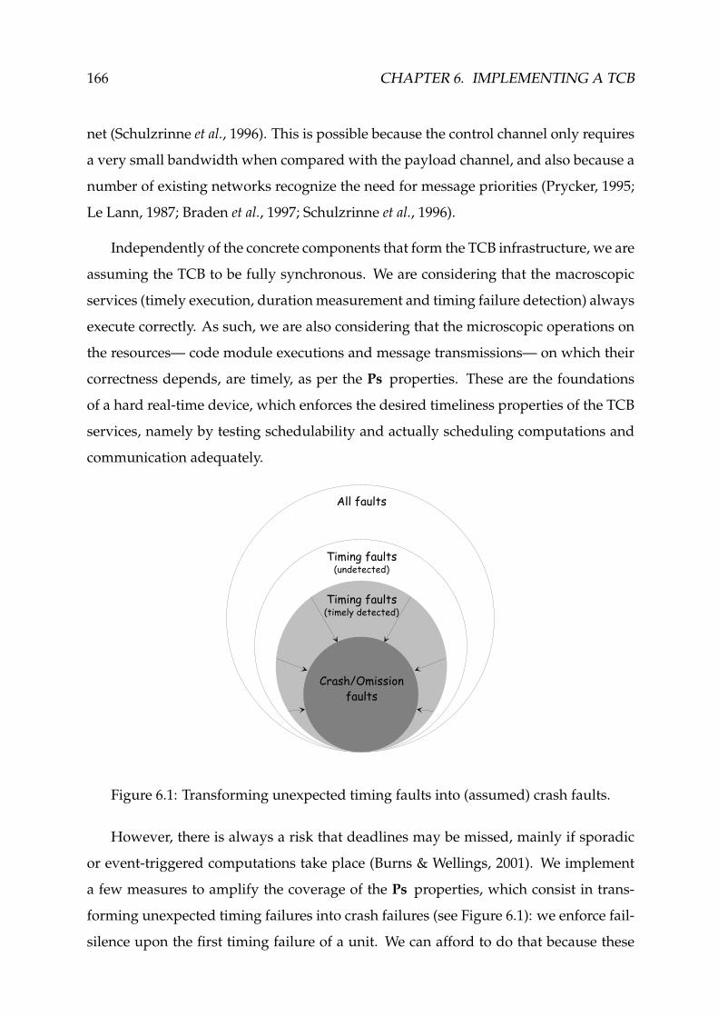
166 CHAPTER 6. IMPLEMENTING A TCB
net (Schulzrinne et al., 1996). This is possible because the control channel only requires
a very small bandwidth when compared with the payload channel, and also because a
number of existing networks recognize the need for message priorities (Prycker, 1995;
Le Lann, 1987; Braden et al., 1997; Schulzrinne et al., 1996).
Independently of the concrete components that form the TCB infrastructure, we are
assuming the TCB to be fully synchronous. We are considering that the macroscopic
services (timely execution, duration measurement and timing failure detection) always
execute correctly. As such, we are also considering that the microscopic operations on
the resources— code module executions and message transmissions— on which their
correctness depends, are timely, as per the Ps properties. These are the foundations
of a hard real-time device, which enforces the desired timeliness properties of the TCB
services, namely by testing schedulability and actually scheduling computations and
communication adequately.
All faults
Timing faults
Crash/Omissionfaults
Timing faults
(undetected)
(timely detected)
Figure 6.1: Transforming unexpected timing faults into (assumed) crash faults.
However, there is always a risk that deadlines may be missed, mainly if sporadic
or event-triggered computations take place (Burns & Wellings, 2001). We implement
a few measures to amplify the coverage of the Ps properties, which consist in trans-
forming unexpected timing failures into crash failures (see Figure 6.1): we enforce fail-
silence upon the first timing failure of a unit. We can afford to do that because these

6.2. ENFORCING SYNCHRONISM PROPERTIES OF THE TCB 167
failures will be rare events, which could however compromise the safety of the system.
Note that we are not allowing timing failures inside the TCB, so these are not tolerance
measures, but safety measures: with this transformation, we bring some unexpected
failures back into the assumed failure mode universe (crash). Note that there may be
other, more sophisticated approaches to improve coverage of a TCB, and there may
be distributed algorithmic approaches to a fault-tolerant TCB. Again, we wish to per-
suade the reader that a baseline implementation of this model can lead to very robust
systems with simple mechanisms. Here is the approach and its validation:
• we only attempt to deal with unexpected failures in time (not in the value) do-
main;
• we assume property Ps2 (clocks) to be always valid; we further assume that the
same reliance can be put on clock-based operations in general, such as reading
the local clock, and have the kernel set up alarms (watchdogs) that trip at a given
time on the local clock;
• as such, we are concerned with the coverage of the more fragile properties: Ps1
(processing) and Ps3 (communication);
• we monitor the termination instants of local computations submitted to the ker-
nel and compare them with the respective deadlines;
• we monitor the delivery instants of messages submitted to the kernel for trans-
mission and compare them with the respective deadlines;
• should any deadline be missed, we enforce fail-silence of the unit observing the
failure.
6.2.1 Improving the coverage of timely processing
To improve the coverage of Ps1 we use the local clock to measure local kernel
execution durations. Recall that we assume that we can place more reliance on the
timeliness of an alarm (watchdog), than on task scheduling. The kernel logs the start
timestamp (Ts) of a time-critical computation with maximum termination time TA, and
sets an alarm for the desired deadline (tdead = Ts + TA). Either the computation ends
in time, that is, until the deadline (Te ≤ tdead) and the alarm does not trip, or else the

168 CHAPTER 6. IMPLEMENTING A TCB
alarm trips and causes the immediate activation of the fail-silence switch, crashing the
whole site.
6.2.2 Improving the coverage of timely communication
A similar principle can be used to improve the coverage of the bounded message
delivery delay property (Ps3). Message delivery delays are measured and compared to
previously specified bounds. Round-trip duration measurement is used, since we are
in the presence of a distributed duration. From a structural point of view, the idea is
to apply the fail-awareness concept to build a fail-aware broadcast (Fetzer & Cristian,
1997b) as the basic kernel communication primitive to serve the TCB control channel.
If a message is not delivered on time, an exception is raised that causes the immediate
activation of the fail-silence switch, crashing the whole site.
Note that we cannot be as aggressive as with processing: we can only act on deliv-
ery of the message and not at the deadline instant. If we acted at the deadline point,
we might be acting on either a crash or a timing failure. Whatever we did might not
be appropriate in the case of crash, since we would be interfering with an assumed
failure mode. For example, since we would crash a TCB that failed to receive a mes-
sage until the maximum delivery time, the crash of a sending TCB (a normal event as
per the assumptions) would cause all recipient TCBs to commit suicide, crashing the
entire system. This would be inappropriate, since the crash of a TCB causes no safety
problems, so we only crash TCBs after they receive a late message. On the other hand,
with our technique, if a sending TCB or the network would cause all of the TCBs to
receive a late message, then all the TCBs would crash as well. However, from a safety
viewpoint this would be appropriate, in order to avoid contamination.
We will show in section 6.4.2.3 that the proposed approach to enforce the synchro-
nism properties of the TCB can be put in practice in a real setting.

6.3. A SIMPLE IMPLEMENTATION USING HARDWARE WATCHDOGS 169
6.3 A simple implementation using hardware watchdogs
In this chapter we have already explained the fundamental reasoning that should
be followed to choose an appropriate TCB solution for a given application, and we
proposed a few techniques to minimize the negative effects of unexpected faults, oc-
curring when the implemented components do not behave as expected. In this section
we present an example of what could perhaps be the most simple instantiation of a
TCB. This is an hardware watchdog.
This simple implementation of a TCB does not provide all the services that should
be available in a “normal” TCB. It only provides a very simple timing failure detection
service that is able to observe one timed action at a time, and also a very simple timely
execution service, which is nothing more than a shut-down trigger (that executes al-
ways the same function).
Nevertheless, as we mentioned in Section 2.3.3.3, the simple availability of an hard-
ware watchdog can be sufficient to perform a fail-safe shutdown when a failure occurs
and, therefore, to implement some sorts of fail-safe applications (e.g., those that do not
need to perform complex shut-down procedures).
In terms of feasibility, this solution can be considered quite good from the point
of view of the coverage achieved. In fact, since hardware watchdogs are typically
available as stand-alone hardware boards that can be plugged into a PC, they are very
small and simple components, with a very low probability of failure.
In essence, these boards fill the role of an autonomous part of the system, with
higher timeliness and robustness, which can not be compromised by any other sys-
tem component. In this sense, the construction principles postulated in Section 3.2 are
implicitly secured: faults external to the watchdog do not affect the latter (shielding),
internal watchdog timers can only be accessed through its interface (interposition), re-
cursive use of (even more accurate or timely) hardware mechanisms for verification
purposes can be envisaged (validation). Note that independently of the synchrony
properties of the whole system, however synchronous it is assumed to be, it is pos-
sible to conceive the existence of an (even more synchronous) watchdog device that

170 CHAPTER 6. IMPLEMENTING A TCB
is used to verify the synchrony properties. And note that this argument can be used
recursively.
6.4 The RT-Linux TCB implementation
In this work, one of our objectives was to demonstrate the practical feasibility of
the TCB, particularly trying to understand the difficulties to enforce the enumerated
constructions principles and evaluate the obtained results relative to the synchrony
assumptions required for the TCB.
To build a TCB proof-of-concept prototype, one including all the basic TCB ser-
vices, we had to choose particular hardware, software and networking components.
We decided to use PC hardware due to its low cost, availability and potentialities.
Furthermore, given that the PC platform is one of the most used for general purpose
applications, the scope of our evaluations results would be wider. Relatively to the
real-time concerns, using PC based hardware is, in principle, not a problem. How-
ever, the crucial factor is how resources are managed, which is an operating system
responsibility.
There are several real-time operating systems for PC platforms, each with its own
features. QNX (Hildebrand, 1992), LynxOS, VxWorks and pSOS+ are all examples of
high-end RTOSs that offer good development environments, are reliable and, above
all, provide all the necessary real-time features. Some of them have concerns with
portability (offering compilers such as GNU gcc and g++) and provide graphical user
interfaces and networking facilities. However, they are commercial products and all
those features are provided at high costs. On the contrary, the real-time extension to
the Linux operating system, RT-Linux (Barabanov & Yodaiken, 1997; Yodaiken & Bara-
banov, 1997), is considered as “free” software and is easily available and increasingly
popular. Therefore, it was chosen for the purposes of our work.
For the communication infrastructure it would be possible to choose a network
with specific characteristics for real-time operation, like ATM (Prycker, 1995) or
CAN (IEEE, 1993), but to our evaluation purposes we have used a Fast-Ethernet (IEEE,

6.4. THE RT-LINUX TCB IMPLEMENTATION 171
1995) network. While the former networks are more expensive and used for particular
applications, the latter is widely used and, within certain conditions, may also provide
the required predictable behavior.
The prototype implementation was done in the context of the MICRA project and
is documented in (Martins, 2002). Therefore, this thesis does not provide any imple-
mentation details: it only refers to the relevant issues and experiences that resulted
from the implementation work, as well as the evaluation results.
6.4.1 RT-Linux system overview
The Real-Time Linux (RT-Linux) system is an extension to Linux, designed to al-
low the execution of real-time tasks in parallel with the normal payload applications.
Linux is available as free software, as well as its extensions, tools and almost every
application. It is highly reliable and widely used in desktop computers and in network
servers.
The effort to provide Unix-like operating systems with real-time capabilities is not
recent. Although several approaches exist, the RT-Linux developers followed a low-
level one, implementing a real-time kernel underneath the operating system and mak-
ing Linux itself to run as another real-time task (Barabanov & Yodaiken, 1997). Since it
runs with the lowest priority, it can be preempted at any time by higher priority tasks.
The key mechanism to achieve this behavior is based on a virtual interrupt scheme
implemented within RT-Linux. This scheme was designed to address the problem of
turning the non-preemptable Linux kernel into a preemptable one. Basically, it consists
in modifying two things: a) the interrupt table vectors, so that they point to RT-Linux
interrupt service routines instead of Linux ones; b) the macros that Linux uses to dis-
able and enable interrupts, cli and sti , so that some RT-Linux code is executed in its
place. This interposition allows RT-Linux to have a complete control over interrupts
and, in particular, to prevent Linux from disabling them for a long, unpredictable time.
Another important aspect of RT-Linux is that it only provides basic services: low-
level task creation, installation of interrupt service routines, and queues for communi-

172 CHAPTER 6. IMPLEMENTING A TCB
cation among the real-time tasks and Linux processes. If any real-time I/O interaction
has to be done, it is necessary to design specific drivers for RT-Linux. For instance, in
TCB implementation it was necessary to redesign the Linux network driver to operate
under RT-Linux (see section 6.4.3).
6.4.2 Implementing TCB services
In order to preserve the synchrony properties Ps1 to Ps3, the TCB module has to be
constructed in the real-time part of RT-Linux. More specifically, the parts that deal with
the API will reside on the non-real-time domain and only the critical parts (periodic ac-
tivities and timely executions) will have to be implemented as real-time tasks. But there
are a number of problems that have to be solved, to obtain a valid TCB implementation.
Namely, it is necessary to find affirmative answers to the following questions:
• Is it possible, under RT-Linux, to accurately predict the execution time of TCB
activities, which is needed for a schedulability analysis?
• Can the TCB handle multiple service requests, arriving at unpredictable instants,
and still be timely and provide timely services?
• Is it possible to implement a RT-Linux TCB, following the TCB construction prin-
ciples (see Section 3.2)?
The remainder of this section discusses these questions, and where appropriate
describes the solutions employed in our implementation.
6.4.2.1 Predictability in RT-Linux
In a system with RT-Linux, where activities belonging to two different synchrony
domains have to share the same hardware resources, there are potential problems of
interference. In fact, in RT-Linux it is possible to observe a phenomena similar to pri-
ority inversion, when an higher priority activity interrupts its execution due to some
event related to an asynchronous activity. Furthermore, the number and frequency of

6.4. THE RT-LINUX TCB IMPLEMENTATION 173
these events is unknown, and cannot be bounded. The effect is that the execution time
of real-time tasks can not be accurately predicted. We identified two situations where
this effect could be observed:
• Data transfers between Linux (asynchronous) devices and the host memory can
be made through DMA. These DMA bursts are out of RT-Linux control and have
priority over the CPU on the access to the system bus. Therefore, if the CPU is
processing a real-time task when a Linux device starts a DMA transfer, the exe-
cution will stop until the DMA operation finishes. For example, when a packet
arrives at a network interface, the card autonomously starts a DMA transfer to
copy the packet into the system memory, interrupting all other activities.
• In RT-Linux systems, hardware devices (including Linux ones) are allowed to
raise interrupt requests that are handled by the virtual interrupt layer of RT-
Linux. Whatever is done in this layer is not important. The fact is that an handler
task is executed, possibly delaying the execution of a real-time activity.
Surprisingly or not, RT-Linux is clearly not a perfect real-time operating system, at
least not for generic PC hardware. Consequently, our approach in terms of implemen-
tation was: a) in first place, try to identify all possible sources of indeterminism and
find particular solutions to avoid their impact; b) try to minimize the negative conse-
quences of unexpected violation of assumptions by employing safety mechanisms that
are activated upon their (expected rare) occurrence.
The overhead caused by sporadic interrupts can be avoided if they are disabled
during the execution of real-time tasks. By doing this, two TCB related (real-time)
interrupts are also disabled: the clock interrupt that drives the RT-Linux scheduler and
the interrupt generated by the network interface card when TCB packets are received.
Fortunately, it is possible to ensure that no clock interrupts have to be raised while
interrupts are disabled (considering typical task lenght). Since the RT-Linux scheduler
uses a one-shot timer to resume real-time tasks precisely when needed, it is sufficient
to construct an admission control module that does not allow tasks to overlap. This
module must handle a periodic task (TFD service) and several sporadic tasks (timely

174 CHAPTER 6. IMPLEMENTING A TCB
execution service and failure handlers). Provided that all task periods and latencies
are known, the module can decide which new tasks can be admitted. The network
interrupt, on the other hand, can occur at any instant. In consequence, real-time actions
that should be performed by the interrupt handler will be delayed until the interrupts
are enabled. The effects of this delay will be discussed afterwards, in this section.
Regarding the problem of DMA bursts, one of the possible solutions could consist
in disabling DMA transfers or modifying the priority assignments to the bus access.
Unfortunately, this would require some architectural hardware modifications, which
is out of the scope of this work. In fact, this would frustrate the basic idea of using
standard PC hardware to implement the TCB. The generic solution to this problem
is implicitly provided by the validation construction principle. By this principle the
TCB will know when a synchrony assumption is violated (e.g. as a result of a DMA
burst), and safety measures may possibly be applied. The validation mechanisms are
discussed in the answer to the third question.
An approach to alleviate the problem of uncertain execution delays, is to add an
extra amount to the maximum task execution time. Note that this amount has always
to be added, at least to account for the scheduling delay variability (typical values
in RT-Linux, using a 120MHz Pentium based PC, are less than 20µs (Barabanov &
Yodaiken, 1997)). Section 6.4.4 provides our own measurements for the scheduling
delay, which were used in the implementation.
6.4.2.2 Handling application requests
The TCB does not impose any restriction on the amount or frequency of service
invocations. Applications may request TCB services whenever they want. Similarly,
they are free to provide whatever service parameters they want. The problem is to
conciliate this flexibility with the limited processing capacity of the TCB.
A simple but effective solution, is to implement an admission control layer in the
TCB interface to filter the requests that cannot be served or that provide incorrect pa-
rameters. The admission procedures, although being part of the TCB interface, have to
be executed in the payload part of the system to avoid the possibility of an uncontrolled

6.4. THE RT-LINUX TCB IMPLEMENTATION 175
access to the real-time part. In the case of startExec , startLocal or send requests,
which may require real-time tasks to be executed, the admission module has to know
the start instant and the deadline of these tasks. If the service can not be provided, the
application will be informed of the denial reasons.
But the admission control layer does not solve all the interfacing problems. In the
above three services, the real-time function specified by the application through pa-
rameter f or handler (see Table 4.1) cannot be verified at run-time. In our RT-Linux
implementation, every real-time function is previously loaded into the kernel space (by
means of the Linux loadable module facilities) and the application only provides a ref-
erence to one of those pre-loaded functions. Each loadable module contains a real-time
function and its estimated worst case execution time (WCET). Since the TCB does not
inspect the function code, neither verifies the correctness of the provided WCET, it is
assumed that users will not intentionally provide incorrect information. Note that the
ability lo load a kernel module is only available to privileged or trusted users. Never-
theless, it is possible that unintentional mistakes occur, like the provision of functions
with run-time errors or the provision of a WCET smaller than the real one. In the
former case, since the error may lead to an uncontrolled and unpredictable system be-
havior, any solution would require specific fault-tolerance techniques. On the other
hand, the provision of a smaller WCET may at worse generate a timing failure. In this
case, the TCB self-checking procedures (that we discuss below) will detect the timing
failure and execute adequate safety procedures.
In the current implementation, we assume that the user is responsible for the cal-
culation of WCET values. However, it would be possible to develop a TCB external
module for off-line code generation and WCET calculation. Such an integrated so-
lution would simplify the development of applications and would solve the above-
mentioned failure problems by ensuring the correctness of all parameters.
6.4.2.3 Enforcing Interposition, Shielding and Validation
Any implementation of a TCB must be ruled by the Interposition, Shielding and Val-
idation construction principles. Fortunately, and perhaps naturally, the RT-Linux ar-

176 CHAPTER 6. IMPLEMENTING A TCB
chitecture greatly simplifies the task. In fact, since RT-Linux is designed to allow the
execution of real-time tasks within an asynchronous system, it must control essential
resources for timeliness (interposition) and must preserve the real-time behavior no
matter what happens in the rest of the system (shielding). Since these two principles
are implicitly granted, our concerns in terms of implementation are essentially focused
on the validation principle.
In fact, the validation principle can be somehow satisfied by following the generic
approach proposed in Section 6.2, which consists in enforcing the synchronism prop-
erties of the TCB. The idea is to implement the necessary measures that allow the TCB
to verify its own timeliness and do whatever is possible when it detects that any of
the assumed property was violated. The measures are carried out using monitoring
mechanisms to which we have called, in this implementation, self-checking mechanisms.
LinuxApplication
LinuxApplication
APITCB Specific Linux
TFD
System HW Resources(Clock, Processor, Interrupts, etc.)
Fail-Silence Switch
Regular Networking Infrastructure
RegularLinux OS
DUREXEC
RT-Linux
Fast-Ethernet Network
RT-Linuxtask
TCB
Self-checkingMechanisms
RT-LinuxDriver
RegularLinux Driver
Figure 6.2: Block diagram of a RT-Linux system with a TCB
As depicted in Figure 6.2, the lower interface of the TCB with the system resources
is under the surveillance of the self-checking mechanisms. As suggested in the figure,
these mechanisms are hooked to a fail-silence switch, an abstraction whose implemen-
tation has the effect of immediately halting the whole site.

6.4. THE RT-LINUX TCB IMPLEMENTATION 177
6.4.3 Implementing communication services
In our RT-Linux implementation, the TCB synchronous communication channel is
based on a physically different network from the one supporting the payload channel.
For the control channel we have used a switched Fast-Ethernet network, exclusively
dedicated to connect local TCBs. The rest of the system is interconnected through a
normal 10Mbit Ethernet network. We refer, once again, that this dual network archi-
tecture is not strictly required by the TCB model. However, it revealed to be a good
practical solution.
The general aspect of the RT-Linux TCB implementation is sketched in figure 6.2.
In this figure, it is possible to observe the several components that exist in the system,
including the dual networking infrastructure.
Given that we have a dedicated network for the control channel, the problem of
achieving predictability is much alleviated. In one hand, since traffic generation is
restricted to the TCB, we can easily control the network load. On the other hand,
by exploiting some specific characteristics of switched Fast-Ethernet networks, it is
possible to eliminate the unpredictability introduced by the Binary Exponential Back-
off collision resolution algorithm of Ethernet networks. The solution simply consists
is avoiding packet collisions. This can be achieved by connecting each port of the
switch to a single station to ensure that at most one adapter may transmit on each
direction of the full-duplex link. Therefore, provided that the switch buffering capacity
is not exceeded (which would introduce additional, possibly unpredictable delays), it
is possible to guarantee a maximum transmission delay for each packet.
However, the end-to-end delivery delay also depends on the time it takes to ac-
tually send and receive messages or, in other words, on the actions performed by the
network driver. This will be discussed next.
6.4.3.1 The TCB network device driver
The standard Linux network driver was not designed for real-time operation.
Therefore, to achieve a real-time behavior within the TCB and the RT-Linux kernel

178 CHAPTER 6. IMPLEMENTING A TCB
itself we had to redesign this driver.
For the port, we used the standard Linux driver for 3COM Ethernet cards (model
3C905b), publicly available as part of the Linux kernel distribution under the name
3c59x.c . Although most of the original code has remained unchanged, like some
functions for booting up, shutting down, or retrieving statistics, the final result is not a
generic driver, but one specifically designed to operate under the TCB.
The crucial modifications took place at the interface between the driver and the
upper levels. The original Linux driver uses an upcall mechanism to deliver incoming
frames to the layer above it. Since this upcall (or message copy) is executed by the
driver interrupt service routine, in RT-Linux this would consume real-time resources.
Furthermore, since messages arrive sporadically the processing overhead would be
unpredictable. The solution is conceptually very simple. When the network interface
card receives a new frame it starts an autonomous DMA transfer and signals the driver
(with an interrupt) when the transfer completes. Then, the driver interrupt service
routine gets a timestamp and acknowledges the interrupt: no copies are done, neither
the message contents are analyzed. Therefore, the execution overhead of the interrupt
routine can be neglected. The driver simply leaves messages in the buffers, waiting for
the upper layer to consume those messages periodically.
This approach requires the consuming rate to be at least equal to the rate of incom-
ing messages. Fortunately, since we have control over the number of messages sent to
the network, it is easy to know the rate of incoming messages. The period of the con-
suming task is calculated in order to prevent buffer overflows and consequent message
losses.
Provided that all the above bounds are enforced, this approach allows the construc-
tion of a real-time communication service under RT-Linux. In fact, it can be guaran-
teed that every message is consumed within a bounded amount of time after it has
been transmitted. This bound depends on the maximum delivery delay (which, for a
given load pattern and message size, can be bounded) and on the period of the con-
suming task. Note that this period should be made as small as possible, since some
TCB parameters (e.g. the maximum failure detection latency) depend on it.

6.4. THE RT-LINUX TCB IMPLEMENTATION 179
6.4.3.2 Device driver services
Beside the management services provided by the standard Linux driver, the RT-
Linux network driver provides the services for transmitting and receiving messages.
The former can be used to reliably broadcast an Ethernet packet to the network and
the latter is used to consume a packet from the device driver buffer.
The transmission service was designed to operate exclusively in broadcast mode
because the TCB always disseminates messages to all other TCBs. When a transmission
request is issued, the driver generates a timestamp that is also sent and that will be
used to measure an upper bound for the delivery delay.
The reliability of the transmission is obtained by letting the service client specify an
assumed network omission degree, and by sending a sufficient number of replicated
messages to mask that omission degree. Note that, as mentioned in Chapter 3, several
solutions for reliable broadcast in synchronous networks exist and could be used here.
However, for practical reasons, and since this is was not one of the main issues of our
work, we have simplified the fault assumptions so that the assumed omission degree
incorporates all faults that could affect the system.
The driver was designed to optimize the replicated transmission: instead of copy-
ing a message into several transmission buffers, it maps several descriptors of the
transmission table to the same memory buffer. On the receiver side, message repli-
cas are not processed by the driver. This would force message contents to be inspected
and, consequently, an increased overhead. Duplicate messages are simply discarded
by the TCB. Note that all message replicas share the same send timestamp, and thus
the maximum delivery delay is calculated for the last replica.
The reception service is used to read messages from driver buffers. When there are
available messages, the service returns all of them along with their reception times-
tamps. These timestamps, and the send timestamps contained in the messages, will be
used by the self-checking mechanism to calculate delivery delays.

180 CHAPTER 6. IMPLEMENTING A TCB
6.4.4 Evaluation results
6.4.4.1 Evaluation scenario
This section presents the results of a few experiments that we have conducted with
the objective of obtaining an intuition of what could be expected, in terms of timeliness,
from the RT-Linux system and from the switched Fast-Ethernet network. The knowl-
edge of concrete timeliness parameters is important to evaluate the appropriateness of
a given infrastructure when certain dependability requirements must be met.
The tests were performed using the experimental infrastructure depicted in Figure
6.3. We used three 500MHz PentiumIII based PCs with the RT-Linux system and a
TCB, interconnected by a 3COM SuperStack II Baseline switch. For the measurements
we used another PC running a special measurement tool (Event Timestamping Tool)
that we have developed. This tool consists of a small kernel booted up from a floppy
disk, which executes a simple program to read events from an input (the parallel port)
and store corresponding timestamps. The granularity of the timestamps depends on
the processor speed, but is typically in the order of a few nanoseconds. A detailed
description of this tool can be found in (Martins & Casimiro, 2000).
RT-Linuxwith TCB
PC with EventTime-Stamping Tool
ETT probes connectedto parallel ports
Fast-Ethernetswitch
Fast-Ethernet links
RT-Linuxwith TCB
RT-Linuxwith TCB
Figure 6.3: Experimental infrastructure.

6.4. THE RT-LINUX TCB IMPLEMENTATION 181
6.4.4.2 Scheduling delay analysis
Our first experience was performed without using the Event Timestamping Tool.
The test, to measure the variability of the scheduling delay in RT-Linux, consisted in
scheduling a real-time task at some instant t and obtaining a timestamp ts (from the
local clock) as soon as the task was released. We measured a maximum scheduling
delay (ts− t) of about 18µs, which is similar to the assumed value of 20µs. The test was
performed under heavy system load conditions (generated by payload applications),
and for task periods ranging from 100µs to 100ms.
We also measured the scheduling delay variability using the Event Timestamping
Tool. We executed a periodic real-time task that did nothing but set up an event on the
parallel port. The variability of scheduling delays, for task periods ranging from 100µs
to 10ms, was lower than 17µs, without load, and lower than 26µs, under heavy load
conditions. This confirms, once again, our expectations.
6.4.4.3 Network delay analysis
To analyze the network behavior we performed a few more tests using the mea-
surement tool. The goal was to validate our expectations about the deterministic char-
acteristics of Fast-Ethernet under controlled load conditions and with switch ports al-
located to unique nodes. Therefore, the tests consisted in measuring message delivery
delays using different message sizes, while increasing the transmission rates until mes-
sage loss started to be observed (when reaching the zero-loss transmission period).
Delivery delays were measured by setting up an event, at the driver level, upon
each message transmission or reception. Since all messages are broadcast, each trans-
mission generates three events (a send and two receive events). We performed eight
experiences, with all three TCBs transmitting simultaneously, for messages with 100,
300, 680 and 1024 bytes, and transmission periods of 10ms and 1ms. Three more ex-
periences were also conducted to evaluate the zero-loss performance of the network.
These were for messages with 300, 680 and 1024 bytes. With messages of 100 bytes
we were not able to reach the zero-loss point, since with only three sending stations too

182 CHAPTER 6. IMPLEMENTING A TCB
much system resources were required.
The value of 1024 bytes ensures that no receive overruns can possibly happen at the
receiver, and that no messages will be lost by this reason. This value was calculated for
receiver input FIFOs with 2048 bytes and for a burst of two messages. In each experi-
ment nearly 30000 message delivery delays were measured. Minimum and maximum
delays are presented in Table 6.1.
Frame size 52µs 113µs 168µs 1ms 10ms100 bytes 42-47 42-49300 bytes 78-221 84-122 83-90680 bytes 153-258 153-178 162-1771024 bytes 221-348 221-359 231-279
Zero-loss periodTransmission period
Table 6.1: Message delivery delays (µs).
Although these were not extensive tests, the results are nevertheless sufficient to
sort out a few conclusions. In the first place, we note that in the experiences corre-
sponding to the zero-loss period, the (input) throughput is near the theoretical maxi-
mum network capacity of 100Mbit/s (for example, 2 flows of 300 byte frames with a
period of 52 µs correspond to near 93Mbit/s).
Without any further details it is possible to observe that delivery delays can be
kept within reasonable intervals, with maximum values not exceeding a few hundred
microseconds. It is also possible to see that lowers bounds for delivery delays tend
to be quite constant because they are determined by the best possible switching delay,
which is constant.
On the other hand, there is a tendency for the length of the intervals (as well as
the upper values) to increase with the amount of traffic sent to the network. This is
due to higher switching delays, caused by extra buffering time when the switch is
operating under heavy load conditions. There are some exceptions, mostly notorious
in the difference between 1024 byte frames with 168µs and 1ms. However, we believe
this exception is not relevant when observing Figure 6.4.

6.4. THE RT-LINUX TCB IMPLEMENTATION 183
1024 byte frames / 168µs period
0
50
100
150
200
250
300
350
400
450
220 240 260 280 300 320 340 360
Delivery delay (µs)
Nu
mb
er o
f fr
ames
Figure 6.4: Delivery delay distribution for large frames at full transmission rate.
This figure shows that there is a quite large queue of delivery delays, which means
that it would be possible to easily end up with somehow different values if new ex-
periences were executed. The relevant issue that can be extracted from this figure is
that although there is this significative dispersion, there is also a clear concentration of
delays around a certain value.
300 byte frames / 52µs period
0102030405060708090
100
70 120 170 220
Delivery delay (µs)
Nu
mb
er o
f fr
ames
Figure 6.5: Delivery delay distribution for small frames at full transmission rate.
In Figure 6.5 it is possible to observe the distribution of delivery delays for one of
the zero-loss period experiences. In terms of probability distribution it is clear that there
is a peak around the value of 130µs, and that the probability of delivery delay values

184 CHAPTER 6. IMPLEMENTING A TCB
above 230µs is extremely low. Given the fact that no message loss is observed in these
conditions, we can conclude that our initial assumptions about the predictability of
Fast-Ethernet networks were indeed quite correct.
Let us now observe the distribution that was obtained in a scenario with low traffic
overhead, in Figure6.6.
300 byte frames / 10ms period
0
2000
4000
6000
8000
10000
12000
14000
82 84 86 88 90 92
Delivery delay (µs)
Nu
mb
er o
f fr
ames
Figure 6.6: Delivery delay distribution for small frames with small transmission rate.
The most immediate observable fact is that the delivery delays appear to be very
predictable around three or four specific values. In fact, when trying to explain this fact
we understood that this was an artificial concentration introduced by the measurement
tool. Therefore, the unique relevant information that we can extract is that almost all
measured delays are included in a small interval of 4µs. This obviously reveals that
the communication is extremely predictable in low load situations.
6.4.4.4 Distributed duration measurement analysis
In the RT-Linux TCB prototype, the distributed duration measurement service was
implemented using the protocol described in Section 4.1.4. Therefore, we also made
several experiences to evaluate the effectiveness of the proposed improved round-trip
technique when compared to the original version proposed by Fetzer (Fetzer & Cris-
tian, 1997a).

6.4. THE RT-LINUX TCB IMPLEMENTATION 185
The tests were performed in our distributed systems laboratory, using the infras-
tructure already described in Section 6.4.4.1. Since our aim was to compare both tech-
niques, we simply needed to generate sequences of messages pairs, for which only two
machines were necessary.
Given that the TCB duration measurement service only implements the improved
technique, for the comparisons we had to extend the service with an implementation of
the original version of the round-trip technique, exactly as described in (Fetzer & Cris-
tian, 1997a). Both implementations run in parallel, using exactly the same input values,
that is, the same send and receive timestamps. They both output pairs of 〈delm, errm〉
values that are used for the comparison.
The experiment consisted in the execution of two applications, a client and a server,
respectively concerned with periodically sending a message, and replying to every re-
ceived message. We have configured the client to send a message every 500ms. There-
fore, in all the figures presented bellow the samples depicted in the X axis correspond
to consecutive measurements obtained with intervals of about 500ms. Note that these
intervals are affected not only by the jitter of the scheduling delay (of the client’s send-
ing task), but also by the jitter of the overall round-trip delay. The specific content of
the messages is irrelevant for the experiment. Both applications were implemented on
top of the TCB duration measurement service. Their only functionality, besides send-
ing and receiving messages, was to store the returned pair of measurement values in a
local file.
We had to set the values of some constants used in the protocol. The drift rate was
set to ρ = 5x10⁻⁶ and we assumed the minimum message transmission delay to be
zero (tmin = 0). The size of the arrays was set to a value larger than two (the number of
used processors).
Relatively to the conditions of the environment during the experiment, in particu-
lar the network and system loads, we have forced a scenario with almost no activity
(typically idle), interleaved with short periods of intensive network utilization. This
unstable behavior is perfectly visible in the figures presented below and, as expected,
allows to clearly observing the improvements obtained with the proposed technique.

186 CHAPTER 6. IMPLEMENTING A TCB
To overload the network we simply used the Unix ping command, with the flood
option enabled.
The applications were executed several times, just to compare the results and verify
their coherence. However, for the purpose of demonstrating our point of view, we have
just selected a representative set of results, one where the differences between the two
techniques can be observed.
0
0,5
1
1,5
2
2,5
3
3,5
4
Measurements in sequential time
Del
ay (
ms)
IMP Error Upper bound RT Error
Figure 6.7: Measurement upper bounds and errors using the improved (IMP) and theoriginal round-trip (RT) techniques.
In Figure 6.7 we compare the error values achieved by both techniques in a series
of consecutive measurements. The upper bound values are also represented to provide
an idea of the system behavior during the experiment. Higher upper bounds typically
correspond to messages transmitted during periods of more intensive traffic. However,
since the ping command was randomly issued, during randomly sized time intervals,
we cannot guarantee a strict correspondence between higher delays and the increased
traffic generated by the ping command.
The most important result that may be observed in this figure is the almost stable
error achieved by the improved technique (IMP Error), in contrast with the variable
error achieved by the other technique (RT Error). This result clearly confirms our ex-
pectations. Note that the RT Error line closely follows the Upper bound line, as dictated
by the original round-trip technique (in this case, since tmin was set to zero, RT Error is
always half of the Upper bound).
To more clearly observe, and compare, the dispersion of the measurement errors

6.4. THE RT-LINUX TCB IMPLEMENTATION 187
0
2
4
6
8
10
12
14
436 444 452 464 477 494 546 635 3426 50161
Estimation error (µs)
Fre
qu
ency
IMP technique RT technique
Figure 6.8: Distribution of estimation errors.
achieved with the two techniques, we analyzed the frequency of each observed er-
ror value, and present the result in Figure 6.8. Error values with no occurrences are
obviously not depicted, which means that the X axis scale is irregular. The higher es-
timation error observed with the IMP technique was near 490µs, while with the RT
technique we observed several error values above 500µs. This result shows that the
improved technique can possibly be used to construct a distributed duration measure-
ment service that ensures a bounded measurement error. Such a service can be very
useful in network monitoring systems, since it allows the establishment of accuracy
bounds for the observations.
0
2
4
6
8
10
Measurements in sequential time
Del
ay (
ms)
IMP Delay Real Delay RT Delay
Figure 6.9: Estimated delays and real (measured) delay.
The accuracy of the estimations obtained with the improved technique can be ob-
served in Figure 6.9. In this figure we compare the real delay of message transmis-
sions, with the delays that were estimated using both techniques. During the periods
of “stability”, when the message transmission delays are low, both techniques seem

188 CHAPTER 6. IMPLEMENTING A TCB
to provide accurate estimations. However, when a higher delay occurs, only the IMP
technique is able to provide accurate estimations.
6.4.4.5 Dependability evaluation
Perhaps worthwhile mentioning are some preliminary results of experiments con-
ducted for the evaluation of the TCB (more precisely, its services) through fault injec-
tion techniques. This work is being developed as a followup to the MICRA project,
in collaboration with a team from the University of Coimbra and from the Superior
Institute of Engineering of Coimbra.
The experiments use a fault-injection tool, the Xception tool (Carreira et al., 1995),
in which specific functionalities were added to inject timing faults and to observe their
effects on the system behavior. Since this is on-going work, we do not provide here
specific details of the experiments nor any conclusive result. However, we can already
point out that timing fault injection raises some particular problems, mainly because it
involves a few time-related aspects, usually irrelevant in other kinds of fault injection,
namely:
• control over the severity of injected faults, which depends on the injected lateness
degree;
• availability of a time base that is independent from the system that is being tested;
• availability of a time base that is more precise and more dependable than the time
source of the target system;
Furthermore, how the code is instrumented in order to guarantee that the possi-
bility of intrusiveness is minimal, is also another issue. After some initial experiments
have been done, it was possible to identify some problems in the experiences itself,
while the execution of the TCB local timing failure detection service (the one that was
tested) has apparently been always correct. The properties of this service, that is, the
timed strong completeness and the timed strong accuracy properties, have been ob-
served to hold in the several test runs that were performed. Nevertheless, further

6.5. SUMMARY 189
experiments still have to be made, which we leave as further work, in order to be able
to make any reasonably conclusion.
6.5 Summary
This chapter was dedicated to the discussion of practical issues concerning the im-
plementation of the TCB. Different implementations can be considered, depending on
the components that are used, but providing necessarily different degrees of depend-
ability. It was shown that the coverage of TCB synchronous assumptions can be im-
proved by employing specific measures to overcome unexpected violations of assumed
bounds. It was shown that the construction of a TCB using COTS components is fea-
sible, but care must be taken to identify the possible impairments to synchrony and
correctly characterize the dependability that may be achieved. Based on experimental
results it was possible to evaluate the achievable timeliness of the computational and
communication platforms and to verify that the proposed round-trip duration mea-
surement protocol indeed improves previous existing solutions.
Notes
The measurements and the RT-Linux implementation presented in this
chapter were obtained with the collaboration of Pedro Martins. These re-
sults and the discussion about the RT-Linux implementation have been pre-
sented in “How to Build a Timely Computing Base using Real-Time Linux”,
Casimiro, Martins and Verıssimo, Proceedings of the “2000 IEEE Workshop
on Factory Communication Systems”, Porto, Portugal, September 2000.
A description of the tool that was used to perform the measurements ap-
pears in a FCUL technical report: “Event Timestamping Tool: a simple
PC based kernel to timestamp distributed events”, Martins and Casimiro,
DI/FCUL TR 00-4, July 2000.

190 CHAPTER 6. IMPLEMENTING A TCB
The measurements of the improved round-trip protocol appear in “Measur-
ing Distributed Durations with Stable Errors”, Casimiro, Martins, Verıssimo
and Rodrigues, Proceedings of the “22nd IEEE Real-Time Systems Sympo-
sium”, London, UK, December 2001.

7Conclusions and
perspectives
This thesis has proposed a new paradigm and a new framework to build timely and
dependable applications in environments of partial synchrony. For several reasons,
including low cost, openness and easy portability, many of the current computing and
networking infrastructures are based on the Internet or on smaller-scale infrastructures
built from COTS components, which cannot provide guarantees in terms of reliability,
synchrony or security. On the other hand, many of the emerging networked services
and applications have timeliness requirements, which call for solutions in the realm of
real-time systems. This raises the challenge of reconciling the needs for timeliness with
the uncertain synchronism of the infrastructure.
An overview of the existing systemic approaches to the problem showed that each
of them treats the problem in its own way, for particular degrees of synchronism of
the environment. This motivated the design of the Timely Computing Base model and
architecture, which provides a generic approach to the problem, for varying degrees
of synchronism, ranging the entire synchrony spectrum. The thesis has presented this
model, its properties and construction principles, and defined the basic services that
a TCB should provide. Because some of these services have a distributed nature, two
protocols, for distributed duration measurement and for timing failure detection, were
also presented.
The way in which applications can benefit from the TCB is by using the TCB
services, provided through an adequate interface, and following appropriate design
methodologies. To illustrate the utility of the TCB, three different techniques to build
dependable applications have been presented and discussed. The remaining question,
191

192 CHAPTER 7. CONCLUSIONS AND PERSPECTIVES
about the feasibility of the proposed model and architecture, was addressed in the final
part of the thesis. Using a TCB prototype built from COTS components, it was possible
to verify that the TCB concept is indeed feasible and adequate when dependability is
an important concern.
Given the above, we believe that the overall objectives of the thesis have been met:
to define a new, more generic model, for partially synchronous environments; to de-
fine the framework and the methodologies to build dependable applications using the
proposed model; to evaluate the proposed solutions.
However, given the huge dimension of the problem addressed here, we obviously
do not expect to have answered all the questions, not even we expect to have com-
prehensively discussed all the issues that came up throughout the thesis. As a matter
of fact, the work presented here can be seen just as a part of a more vast work con-
cerning the treatment of uncertainty not only to achieve timeliness, but also to achieve
security, reliability or performance. It is not a coincidence that the Navigators group is
currently designing efficient byzantine-resilient protocols (Correia et al., 2002b) based
on the Trusted Timely Computing Base (TTCB) model (Correia et al., 2002a), which
extends the TCB model with additional fundamental services for trust and security.
Because of the above, and since we are convinced that there will be excellent oppor-
tunities to continue, improve and expand the work presented here, we now provide a
list of open issues and topics for future work:
• Define a complete set of classes of timing failure detectors. The TCB model de-
fines the properties of a perfect Timing Failure Detector (pTFD), which we clas-
sified as sufficient to dependably build the several classes of applications that
were considered. However, it remains to see if it is possible to define other
TFD classes (similarly to what have been done by Chandra & Toueg (Chandra
& Toueg, 1996)), satisfying strictly weaker properties but still serving the same
purposes. Really interesting would be to find the weakest timing failure detector
which would allow, for instance, to apply the paradigm for generic timing fault
tolerance using a replicated state machine based server described in Section 5.6.

193
• Show that a crash failure detector is a particular instance of a timing failure detec-
tor. It is well known (and it was mentioned in the thesis) that crash failures are a
particular subset of timing failures: a component producing infinitely many tim-
ing failures with infinite lateness degree can be detected has crashed. Therefore,
it would be interesting to formally demonstrate that there is a transformation
which takes a timing failure detector and produced a crash failure detector.
• Propose architectural or engineering alternatives to deal with scalability prob-
lems. The TCB model assumes that there exists a TCB module in each local site,
which may cause serious scalability problems from the point of view of the num-
ber of participants (we do not consider geographic scale to be a serious problem).
Therefore, the possibility of considering different approaches, for instance using
hierarchies of TCB domains with different dependability guarantees or defining
TCB servers to be shared by several nodes, deserves to be investigated.
• Refine the proposed paradigms for timing fault tolerance, or propose new ones.
We have defined a few classes of applications, which served our purposes of
demonstrating the utility of the TCB and its services. However, it may be possible
to identify other typical applications classes for which new paradigms would
make sense. On the other hand, we believe there is ground to apply mechanism
such as replication for various interaction models, which would yield different
paradigms for timing fault tolerance.
• Develop middleware components over the TCB and its services. For example, the
provision of a middleware service offering a timed form of consensus would cer-
tainly be highly valuable for a number of applications. Following the perspective
of offering powerful time related tools to application developers, the integration
of several middleware services, such as the QoS coverage service described in
this thesis or a timed event service, would be extremely benefic.
• Perform additional evaluation tests, namely using fault injection techniques. We
have already mentioned that the RT-Linux prototype is being evaluated through
fault injection in the scope of the MICRA project. Several questions and problems
have been raised in the course of that work, which make we think that this is an

194 CHAPTER 7. CONCLUSIONS AND PERSPECTIVES
area of research that deserves to be further explored. For example, more can be
done not only in what concerns the definition of adequate mechanisms and tech-
niques for the injection of timing faults, but also in what concerns the evaluation
of the injection results.
• Study the possibility of implementing the TCB in different infrastructures. The
use of the TCB model and architecture have been suggested in the aim of the
CORTEX project, which envisages the use of wireless networks as one of the pos-
sible networks supporting CORTEX applications. Therefore, it makes sense to
investigate the challenges posed by the use of wireless technologies to the im-
plementation of control channels, and study possible solutions for the problems
encountered. We must mention that some work is already being done in this
direction.
• Develop example applications to evaluate the practical utility of the TCB and of
the middleware services developed over it. One of the objectives of the CORTEX
project is to construct small demonstrator prototypes. Hence, we intend to de-
velop some example applications to demonstrate how the availability of a TCB
can be useful.

AProofs
Theorem 1: Given any message m, the upper bound determined for the message delivery delay
of m using the improved technique is equal to the upper bound determined using the round-trip
technique, tIMPmax (m) = tRT
max(m).
Proof:
We use Figure A.1 to visually guide this proof. Consider the depicted sequence of
messages. We will show that the theorem is valid for message mk+1, and that it can be
generalized to any other message.
We will start by showing that mk+1 can be the first message in some sequence that
might possibly have tIMPmax < tRT
max — all previous messages in the sequence are guaran-
teed to have the same upper bound using any of the techniques — and we will show
that in spite of this possibility the upper bounds are nevertheless equal. Since the same
reasoning can recursively be applied to the first subsequent message for which it might
also be possible to have tIMPmax < tRT
max, the theorem can be generalized for every subse-
quent message.
p
q
mk
A
mk-1
B C
D E
FS
R
mk-2 mk+1
Figure A.1: Upper bound preservation for mk+1.
Let us assume that the message pair 〈mk, mk+1〉 is the one used to determine the
upper bounds (mk has been considered by p the “best” message so far). The equations
195

196 APPENDIX A. PROOFS
that provide the upper bounds for mk+1 follow from (4.5) and (4.9):
tRTmax(mk+1) = (F − C)(1 + ρ)− (E −D)(1− ρ)− tmin
tIMPmax (mk+1) = (F − C)(1 + ρ)− (E −D)(1− ρ)− (t(mk)− ε(mk))
For t(mk)− ε(mk) = tmin it immediately follows that tIMPmax (mk+1) = tRT
max(mk+1). We
are left with the possibility that
t(mk)− ε(mk) > tmin (A.1)
In this case it is reasonable to believe that tIMPmax (mk+1) may be lower than tRT
max(mk+1),
which we will prove to be untrue.
Now observe that for inequality (A.1) to be possible, it is necessary to consider
the existence of a message pair preceding mk in the same sequence. We assume this
message pair to be 〈mk−1, mk−2〉, as depicted in Figure A.1. Furthermore, we assume
these two messages to be the first ones in the sequence, so that mk+1 is clearly the first
message for which tIMPmax < tRT
max may be possible. With these assumptions it is also clear
that the theorem holds for all messages preceding mk+1. Let us write the upper bound
for t(mk−1) (applying (4.5)):
tmax(mk−1) = (B − S)(1 + ρ)− (A−R)(1− ρ)− tmin (A.2)
Given that tIMPmin (mk) = t(mk)− ε(mk) > tmin, we can use expression (4.10) to write
the following:
tIMPmin (mk) > tmin ⇔ (D − A)(1− ρ)− (C −B)(1 + ρ)− (t(mk−1) + ε(mk−1)) > tmin ⇔
⇔ (D − A)(1− ρ)− (C −B)(1 + ρ)− tmax(mk−1) > tmin ⇔
⇔ (D − A)(1− ρ)− (C −B)(1 + ρ)−
− (B − S)(1 + ρ) + (A−R)(1− ρ) + tmin > tmin ⇔
⇔ (D −R)(1− ρ)− (C − S)(1 + ρ) + tmin > tmin ⇔
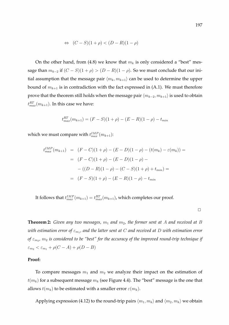
197
⇔ (C − S)(1 + ρ) < (D −R)(1− ρ)
On the other hand, from (4.8) we know that mk is only considered a “best” mes-
sage than mk−2 if (C − S)(1 + ρ) > (D − R)(1 − ρ). So we must conclude that our ini-
tial assumption that the message pair 〈mk, mk+1〉 can be used to determine the upper
bound of mk+1 is in contradiction with the fact expressed in (A.1). We must therefore
prove that the theorem still holds when the message pair 〈mk−2, mk+1〉 is used to obtain
tRTmax(mk+1). In this case we have:
tRTmax(mk+1) = (F − S)(1 + ρ)− (E −R)(1− ρ)− tmin
which we must compare with tIMPmax (mk+1):
tIMPmax (mk+1) = (F − C)(1 + ρ)− (E −D)(1− ρ)− (t(mk)− ε(mk)) =
= (F − C)(1 + ρ)− (E −D)(1− ρ)−
− ((D −R)(1− ρ)− (C − S)(1 + ρ) + tmin) =
= (F − S)(1 + ρ)− (E −R)(1− ρ)− tmin
It follows that tIMPmax (mk+1) = tRT
max(mk+1), which completes our proof.
2
Theorem 2: Given any two messages, m1 and m2, the former sent at A and received at B
with estimation error of εm1 , and the latter sent at C and received at D with estimation error
of εm2 , m2 is considered to be “best” for the accuracy of the improved round-trip technique if
εm2 < εm1 + ρ(C − A) + ρ(D −B)
Proof:
To compare messages m1 and m2 we analyze their impact on the estimation of
t(mk) for a subsequent message mk (see Figure 4.4). The “best” message is the one that
allows t(mk) to be estimated with a smaller error ε(mk).
Applying expression (4.12) to the round-trip pairs 〈m1, mk〉 and 〈m2, mk〉we obtain

198 APPENDIX A. PROOFS
the following:
εm1(mk) = ε(m1) + ρ(F − A) + ρ(E −B)
= ε(m1) + ρ(F − C) + ρ(C − A) + ρ(E −D) + ρ(D −B)
εm2(mk) = ε(m2) + ρ(F − C) + ρ(E −D)
Hence, m2 is better than m1 if:
εm2(mk) < εm1(mk) ⇒ ε(m2) + ρ(F − C) + ρ(E −D) <
ε(m1) + ρ(F − C) + ρ(C − A) + ρ(E −D) + ρ(D −B)⇔
⇔ ε(m2) < ε(m1) + ρ(C − A) + ρ(D −B)
2
Lemma 1: Given a historyH(T ) containing a finite initial number of executions n0, the TCB
can compute the probability density function pdf of the duration T bounded by T and there
exists a pdev0 known and bounded, such that for any P = pdf(T ), and p the actual probability
of T , it is |p− P | ≤ pdev0
Proof sketch:
From service TCB2, the TCB is capable of measuring all durations T (i) in any his-
tory H. For a history H(T ), T (i) are the observed durations representing the specified
duration bound T . For any given actual distribution of T , a discrete probability dis-
tribution function pdf built with n0 observations T (i), subjected to the TCB duration
measurement error TDURmin, represents T with an error of pdev0 (Feller, 1971). 2
Lemma 2: Given pdfi−1(T ), of duration T in H(T ), and given any immediately subsequent
n executions, the TCB can compute pdfi(T ) and there exists a pdev known and bounded, such
that for any P = pdfi(T ), and p the actual probability of T , it is |p− P | ≤ pdev
Proof sketch:

199
From Lemma 1, the TCB is capable of recomputing pdf(T ) for any additional n
(consider n′0 = n0 + n). Then, pdf must preserve a bounded error, event in the presence
of large deviations: for any T with actual probability of p, and any n, there is a subset
ni−1 of the last executions of the original history H, and an adequate function (Wold,
1965), such that P = pdfi(T ) recomputed with the ni−1 +n observations has a bounded
error pdev from p. 2
Theorem 3: An application A ∈ T ε using a TCB and the coverage-stabilization algorithm has
coverage stability
Proof:
From Definition 2, we see that any T derived from any property P of A, is not an
invariant, and as such, the correctness of A does not depend of the absolute value of
any T , but rather on a ’correct’ value of the latter. In consequence, any T can be mod-
ified, namely with the intent of achieving coverage stability. From lemmata 1 and 2,
and the discussion that followed about the coverage-stabilization algorithm, we see
that for any property P with assumed coverage PP , any historyH(TP) derived from P
has coverage stability. By induction on every P ∈ PA, and by Definition 1, application
A has coverage stability. 2
Theorem 4: An application A ∈ Fσ using a TCB has no-contamination
Proof:
Consider a timing failure in H(T ) derived from timeliness property P ∈ A. By
Lemmata 3 and 4, we see that for any bound T established as per the error cancella-
tion rule, failures are not wrongly detected, and any failure of X ∈ H(T ), is detected
until T has elapsed. Consider this instant as corresponding to tFS at the latest, when
fail-safe switching is done, by Definition 4. Then, if up to instant tFS (correspond-
ing to detection threshold T ) there was no evidence of failure in H(T ), the system
was correct. Since the system halts at this point, the corresponding history H(T ) has
no-contamination, by the respective definition. The effect of the failure could not prop-
agate, and in consequence, all other histories have no-contamination. In consequence,
any safety property that was true before tFS , will remain true after halting, by Defini-

200 APPENDIX A. PROOFS
tion 4. Then, by Definition 3, application A has no-contamination. 2
Theorem 5: An application A ∈ T σ using a TCB has no-contamination
Proof:
If A ∈ T σ, then no histories are derived from safety properties. In consequence,
any historyH(T ) has to have been derived from a timeliness property. By definition of
no-contamination, such histories have no-contamination. By Definition 3, application
A has no-contamination. 2

References
ABDELZAHER, T. F., & SHIN, K. G. 1998 (June). End-host Architecture for QoS-
Adaptive Communication. In: Proceedings of the 4th IEEE Real-Time Technology and
Applications Symposium.
ABDELZAHER, T. F., ATKINS, E. M., & SHIN, K. G. 1997. QoS Negotiation in Real-
Time Systems and Its Application to Automated Flight Control. In: Proceedings of
the 3rd IEEE Real-Time Technology and Applications Symposium. Montreal, Canada:
IEEE Computer Society Press.
ABRAMS, M., JAJODIA, S., & PODELL, H. (eds). 1995. Information Security. IEEE CS
Press.
AGUILERA, M., CHEN, W., & TOUEG, S. 1997. Heartbeat: a timeout-free failure de-
tector for quiescent reliable communication. Pages 126–140 of: Proceedings of the
11th International Workshop on Distributed Algorithms (WDAG ’97),. Lecture Notes
in Computer Science. Saarbruecken, Germany: Springer-Verlag.
ALARI, G., & CIUFFOLETTI, A. 1997. Implementing a Probabilistic Clock Synchroniza-
tion Algorithm. Journal of Real-Time Systems, 13(1), 25–46.
ALLEN, A. O. 1990. Probability, Statistics, and Queueing theory with Computer Science
Applications. 2nd edn. Academic Press.
ALMEIDA, C. 1998 (Jan.). Comunication in Quasi-Synchronous Systems: Providing Support
a for Dynamic Real-Time Applications. Ph.D. thesis, Instituto Superior Tecnico. (in
Portuguese).
201

202 REFERENCES
ALMEIDA, C., & VERISSIMO, P. 1996 (June). Timing Failure Detection and Real-Time
Group Communication in Quasi-Synchronous Systems. In: Proceedings of the 8th
Euromicro Workshop on Real-Time Systems.
ALMEIDA, C., & VERISSIMO, P. 1998 (Dec.). Using light-weight groups to handle tim-
ing failures in quasi-synchronous systems. Pages 430–439 of: Proceedings of the 19th
IEEE Real-Time Systems Symposium.
AMIR, Y., MOSER, L., SMITH, P. MELLIAR, AGARWAL, D., & CIARFELLA, P. 1993
(May). Fast Message ordering and membership using a logical token-passing ring.
Pages 551–560 of: Proceedings of the 13th International Conference on Distributed Com-
puting Systems.
ANCEAUME, E., & PUAUT, I. 1998 (Oct.). Performance Evaluation of Clock Synchroniza-
tion Algorithms. Tech. rept. PI-1208. IRISA, Campus de Beaulieu, 35042 Rennes
Cedex, France.
ANCEAUME, E., CHARRON-BOST, B., MINET, P., & TOUEG, S. 1995 (Nov.). On the
Formal Specification of Group Membership Services. Tech. rept. RR-2695. INRIA, Do-
maine de Voluceau, Rocquencourt, B.P. 105, 78153 LE CHESNAY Cedex, France.
ANCEAUME, E., CABILLIC, G., CHEVOCHOT, P., & PUAUT, I. 1998 (May). HADES: A
Middleware Support for Distributed Safety-Critical Real-Time Applications. In:
Proceedings of the 18th International Conference on Distributed Computing Systems
(ICDCS ’98).
ARVIND, K. 1994. Probabilistic clock synchronization in distributed systems. IEEE
Transactions on Parallel and Distributed Systems, 5(5), 474–487.
AURRECOECHEA, C., CAMPBELL, A. T., & HAUW, L. 1998. A Survey of QoS Architec-
tures. Multimedia Systems Journal - Special Issue on QoS Architecture, 6(3), 138–151.
BABAOGLU, O., & DRUMMOND, R. 1985. Streets of Byzantium: Network Architectures
for Fast Reliable Broadcasts. IEEE Transactions on Software Engineering, SE-11(6),
546–554.

REFERENCES 203
BAGCHI, S., WHISNANT, K., KALBARCZYK, Z., & IYER, R. K. 1998 (Oct.). Chameleon:
A Software Infrastructure for Adaptive Fault Tolerance. In: Proceedings of the 17th
IEEE Symposium on Reliable Distributed Systems.
BARABANOV, M., & YODAIKEN, V. 1997. Real-Time Linux. Linux Journal, Mar.
http://rtlinux.cs.nmt.edu/rtlinux/papers/lj.ps.
BERTIER, M., MARIN, O., & SENS, P. 2002 (June). Implementation and performance
evaluation of an adaptable failure detector. Pages 354–363 of: Proceedings of the 2002
International Conference on Dependable Systems & Networks.
BIRMAN, K. P. 1985 (Dec.). Replication and Fault Tolerance in the ISIS System. Pages
79–86 of: Proceedings of the 10th ACM Symposium on Operating Systems Principles.
BIRMAN, K. P., & JOSEPH, T. A. 1985. Reliable Communication in the Presence of
Failures. ACM Transactions on Computer Systems, 5(1), 47–76.
BLAKE, S., BLACK, D., CARLSON, M., DAVIES, E., WANG, Z., & WEISS, W. 1998
(Dec.). An Architecture for Differentiated Services.
BRADEN, R., CLARK, D., & SHENKER, S. 1994 (June). Integrated Services in the Internet
Architecture: an Overview.
BRADEN, R., ZHANG, L., BERSON, S., HERZOG, S., & JAMIN, S. 1997 (Sept.). RFC
2205: Resource ReSerVation Protocol (RSVP) — Version 1 Functional Specification.
BRAND, R. 1995. Iso-Ethernet: Bridging the gap from WAN to LAN. Data Communica-
tions, July.
BURNS, A., & WELLINGS, A. 2001. Real-Time Systems and Programming Languages. 3rd
edn. International Computer Science Series. Addison-Wesley.
BUSSE, I., DEFFNER, B., & SCHULZRINNE, H. 1996. Dynamic QoS Control of Multi-
media Applications based on RTP. Computer Communications, 19(1).
CAMPBELL, A., & COULSON, G. 1996 (Nov.). A QoS adaptive transport system: De-
sign, implementation and experience. Pages 117–128 of: Proceedings of the Fourth
ACM Multimedia Conference.

204 REFERENCES
CAMPBELL, A. T. 1996 (Jan.). A Quality of Service Architecture. Ph.D. thesis, Computing
Department – Lancaster University.
CARREIRA, J., MADEIRA, H., & SILVA, J. G. 1995. Xception: Software Fault Injection
and Monitoring in Processor Functional Units. Pages 135–149 of: Proceedings of the
Working Conference on Dependable Computing for Critical Applications (DCCA’95).
CARTER, W, & SCHNEIDER, P. 1968. Design of dinamically checked computers. Pages
878–883 of: Proceedings of IFIP´68 World Computer Congress.
CASIMIRO, A., & VERISSIMO, P. 1999a (Apr.). Timing Failure Detection with a Timely
Computing Base. In: Proceedings of the European Research Seminar on Advances in
Distributed Systems.
CASIMIRO, A., & VERISSIMO, P. 1999b (Nov.). Timing Failure Detection with a Timely
Computing Base. DI/FCUL TR 99–8. Department of Computer Science, University
of Lisbon.
CASIMIRO, A., & VERISSIMO, P. 2001a (Oct.). Using the Timely Computing Base for
Dependable QoS Adaptation. Pages 208–217 of: Proceedings of the 20th IEEE Sympo-
sium on Reliable Distributed Systems.
CASIMIRO, A., & VERISSIMO, P. 2001b (July). Using the Timely Computing Base for
Dependable QoS Adaptation. DI/FCUL TR 01–3. Department of Computer Science,
University of Lisbon.
CASIMIRO, A., & VERISSIMO, P. 2002. Generic Timing Fault Tolerance using a Timely
Computing Base. Pages 27–36 of: Proceedings of the 2nd International Conference on
Dependable Systems and Networks. Washington DC, USA: IEEE Computer Society
Press.
CASIMIRO, A., MARTINS, P., & VERISSIMO, P. 2000 (Sept.). How to Build a Timely
Computing Base using Real-Time Linux. Pages 127–134 of: Proc. of the 2000 IEEE
Workshop on Factory Communication Systems.

REFERENCES 205
CASIMIRO, A., MARTINS, P., VERISSIMO, P., & RODRIGUES, L. 2001a (Dec.). Measur-
ing Distributed Durations with Stable Errors. Pages 310–319 of: Proceedings of the
22nd IEEE Real-Time Systems Symposium.
CASIMIRO, A., MARTINS, P., VERISSIMO, P., & RODRIGUES, L. 2001b (July). Mea-
suring Distributed Durations with Stable Errors. DI/FCUL TR 01–6. Department of
Computer Science, University of Lisbon.
CHANDRA, T., & TOUEG, S. 1991 (Aug.). Unreliable Failure Detectors for Reliable
Distributed Systems. Pages 325–340 of: Proceedings of the 10th ACM Symposium on
Principles of Distributed Computing. ACM, Montreal, Quebec, Canada.
CHANDRA, T., & TOUEG, S. 1996. Unreliable Failure Detectors for Reliable Distributed
Systems. Journal of the ACM, 43(2), 225–267.
CHANDRA, T., HADZILACOS, V., TOUEG, S., & CHARRON-BOST, B. 1996a (May). On
the Impossibility of Group Membership. Pages 322–330 of: Proceedings of the 15th
ACM Symposium on Principles of Distributed Computing. ACM, Philadelphia, USA.
CHANDRA, T., HADZILACOS, V., & TOUEG, S. 1996b. The weakest failure detector for
solving consensus. Journal of the ACM, 43(4), 685–722.
CHATTERJEE, S., SYDIR, J., SABATA, B., & LAWRENCE, T. 1997 (Aug.). Modeling Ap-
plications for Adaptive QoS-based Resource Management. In: Proceedings of the
2nd IEEE High Assurance Engineering Workshop.
CHEN, W., TOUEG, S., & AGUILERA, M. 2000. On the Quality of Service of Failure
Detectors. Pages 191–200 of: Proceedings of the International Conference on Dependable
Systems and Networks. New York City, USA: IEEE Computer Society Press.
CORREIA, M., VERISSIMO, P., & NEVES, N. F. 2002a (Oct.). The Design of a COTS
Real-Time Distributed Security Kernel. In: Fourth European Dependable Computing
Conference.
CORREIA, M., LUNG, L. C., NEVES, N. F., & VERISSIMO, P. 2002b (Oct.). Efficient
Byzantine-Resilient Reliable Multicast on a Hybrid Failure Model. In: Proc. of the
21th IEEE Symposium on Reliable Distributed Systems.

206 REFERENCES
COSQUER, F., RODRIGUES, L., & VERISSIMO, P. 1995 (Oct.). Using Tailored Failure
Suspectors to Support Distributed Cooperative Applications. Pages 352–356 of:
Proceedings of the 7th International Conference on Parallel and Distributed Computing
and Systems. IASTED.
CRISTIAN, F. 1989. Probabilistic Clock Synchronization. Distributed Computing, 3(3),
146–158.
CRISTIAN, F. 1996. Synchronous and Asynchronous Group Communication. Commu-
nications of the ACM, 39(4), 88–97.
CRISTIAN, F., & FETZER, C. 1994. Probabilistic Internal Clock Synchronization. Pages
22–31 of: Proceedings of the 13th Symposium on Reliable Distributed Systems. Dana
Point, California, USA: IEEE Computer Society Press.
CRISTIAN, F., & FETZER, C. 1999. The Timed Asynchronous Distributed System
Model. IEEE Transactions on Parallel and Distributed Systems, June, 642–657.
CRISTIAN, F., AGHILI, H., STRONG, R., & DOLEV, D. 1985. Atomic Broadcast: From
Simple Message Diffusion to Byzantine Agreement. In: Fifteenth International Con-
ference on Fault Tolerant Computing, Ann Arbor, Michigan. IEEE Computer Society
Press.
CRISTIAN, F., AGHILI, H., STRONG, R., & DOLEV, D. 1995. Atomic Broadcast: From
Simple Message Diffusion to Byzantine Agreement. Information and Computation,
118(1), 158–179.
CUKIER, M., REN, J., SABNIS, C., HENKE, D., PISTOLE, J., SANDERS, W., BAKKEN,
D., BERMAN, M., KARR, D., & SCHANTZ, R. 1998 (Oct.). AQuA: An Adaptive
Architecture That Provides Dependable Distributed Objects. In: Proceedings of the
17th IEEE Symposium on Reliable Distributed Systems.
DELPORTE-GALLET, C., FAUCONNIER, H., & GUERRAOUI, R. 2002 (June). A realis-
tic look at failure detectors. Pages 345–353 of: Proceedings of the 2002 International
Conference on Dependable Systems & Networks.

REFERENCES 207
DENG, Z., & LIU, J. W.-S. 1997 (Dec.). Scheduling real-time applications in an open
environment. Pages 308–319 of: Proceedings of the 18th IEEE Real-Time Systems Sym-
posium.
DOLEV, D., DWORK, C., & STOCKMEYER, L. 1983 (Nov.). On the Minimal Synchronism
Needed for Distributed Consensus. In: 24th Annual Symposium on Foundations of
Computer Science. IEEE, Tucson, USA.
DOLEV, D., KRAMER, S., & MALKI, D. 1993 (June). Early Delivery Totally Or-
dered Multicast in Asynchronous Environments. Pages 544–553 of: LAPRIE, JEAN-
CLAUDE (ed), Digest of Papers, The 23th Annual International Symposium on Fault-
Tolerant Computing.
DWORK, C., LYNCH, N., & STOCKMEYER, L. 1988. Consensus in the Presence of Partial
Synchrony. Journal of the ACM, 35(2), 288–323.
ESSAME, D., ARLAT, J., & POWELL, D. 1999 (Jan.). PADRE: A Protocol for Asymmetric
Duplex REdundancy. Pages 213–232 of: Proceedings of the Seventh IFIP International
Working Conference on Dependable Computing for Critical Applications.
FELLER, W. 1971. An Introduction to Probability Theory and its Applications. 2nd edn.
New York: John Wiley & Sons.
FERGUSON, P., & HUSTON, G. 1998. Quality of Service: Delivering QoS on the internet
and in corporate networks. John Wiley & Sons Inc.
FERRARI, D. 1990 (Oct.). Client Requirements for Real-Time Communication Services.
In: Proceedings of the International Conference on Information Technology. also IEEE
Communications Magazine, 28(11):65–72, November 1990.
FETZER, C. 1997. Fail-Awareness in Timed Asynchronous Systems. Ph.D. thesis, University
of California, San Diego.
FETZER, C. 1999 (Apr.). A comparision of the Timed Asynchronous Systems and Asyn-
chronous Systems with Failure Detectors. In: Third European Research Seminar on
Advances in Distributed Systems.

208 REFERENCES
FETZER, C. 2001 (Apr.). Enforcing Perfect Failure Detection. Pages 350–357 of: Proceed-
ings of the 21st IEEE International Conference on Distributed Computing Systems.
FETZER, C., & CRISTIAN, F. 1995 (Dec.). On the Possibility of Consensus in Asyn-
chronous Systems. In: Proceedings of the 1995 Pacific Rim International Symposium
on Fault-Tolerant Systems.
FETZER, C., & CRISTIAN, F. 1996a. Fail-Aware Failure Detectors. In: Proceedings of
the 15th Symposium on Reliable Distributed Systems. Niagara-on-the-Lake, Canada:
IEEE Computer Society Press.
FETZER, C., & CRISTIAN, F. 1996b (Nov.). A Fail-Aware Membership Service. Tech. rept.
CS96-503. University of California, San Diego.
FETZER, C., & CRISTIAN, F. 1996c (May). Fail-Awareness in Timed Asynchronous
Systems. Pages 314–321a of: Proceedings of the 15th ACM Symposium on Principles of
Distributed Computing. ACM, Philadefphia, USA.
FETZER, C., & CRISTIAN, F. 1997a (Apr.). A Fail-Aware Datagram Service. In: Proc. of
the 2nd Workshop on Fault-Tolerant Parallel and Distributed Systems.
FETZER, C., & CRISTIAN, F. 1997b (June). Fail-Awareness: An Approach to Construct
Fail-Safe Applications. Pages 282–291 of: Digest of Papers, The 27th Annual Interna-
tional Symposium on Fault-Tolerant Computing.
FETZER, C., & CRISTIAN, F. 1997c. Integrating External and Internal Clock Synchro-
nization. Journal of Real-Time-Systems, 12(2), 123–171.
FISCHER, M. J., LYNCH, N. A., & PATERSON, M. S. 1985. Impossibility of Distributed
Consensus with One Faulty Process. Journal of the ACM, 32(2), 374–382.
FOSTER, I., SANDER, V., & ROY, A. 2000 (June). A Quality of Service Architecture that
Combines Resource Reservation and Application Adaptation. Pages 181–188 of:
Proceedings of the Eighth International Workshop on Quality of Service.
GOPAL, A., & TOUEG, S. 1991. Inconsistency and Contamination. Pages 257–272 of:
Proceedings of the 10th Annual ACM Symposium on Principles of Distributed Comput-
ing. Montreal, Quebec, Canada: ACM Press.

REFERENCES 209
HALPERN, J., SIMONS, B., STRONG, R., & DOLEV, D. 1984 (Aug.). Fault-tolerant clock
synchronization. Pages 89–102 of: Proceedings of 3rd ACM Symposium on Principles
of Distributed Computing. ACM SIGPLAN/SIGOPS, Vancouver, Canada.
HERMANT, J.-F., & LANN, G. LE. 2002. Asynchronous Uniform Consensus in Real-
Time Distributed Systems. IEEE Transactions on Computers, Special Issue on Asyn-
chronous Real-Time Distributed Systems, 51(8), 931–944.
HILDEBRAND, D. 1992 (Apr.). An architectural overview of QNX. Pages 113–126 of:
USENIX Workshop on Micro-Kernels and Other Kernel Architectures.
HOPKINS, A., SMITH, T., & LALA, J. 1978. FTMP - A highly reliable fault-tolerant
multiprocessor for aircraft. Proceedings of the IEEE, 66(10), 1221–1239.
HORNING, J.J., LAUER, H.C., MELLIAR-SMITH, P.M., & RANDALL, B. 1974. A Pro-
gram Structure for Error Detection and Recovery. Lecture Notes in Computer Science,
16, 171–187.
IEEE. 1993 (Nov.). Road Vehicles - Interchange of Digital Information - Controller Area
Network (CAN) for High-Speed Communication, ISO 11898.
IEEE. 1995 (Mar.). IEEE 802.3u Standard. Local and Metropolitan Area Networks-
Supplement - Media Access Control (MAC) Parameters, Physical Layer, Medium At-
tachment Units and Repeater for 100Mb/s Operation, Type 100BASE-T. Supplement to
IEEE Std 802-3.
JAHANIAN, F. 1994. Fault Tolerance in Embedded Real-Time Systems. Lecture Notes in
Computer Science, 774, 237–249.
JENSEN, E. D., & NORTHCUTT, J. D. 1990. Alpha: A non-proprietary os for large,
complex, distributed real-time systems. Pages 35–41 of: Proceedings of the IEEE
Workshop on Experimental Distributed Systems. Huntsville, Alabama, USA: IEEE
Computer Society Press.
KIM, K.H. 1984 (May). Distributed Execution of Recovery Blocks: An Approach to
Uniform Treatment of Hardware and Software Faults. Pages 526–532 of: Proceedings
of the Fourth International Conference on Distributed Computing Systems.

210 REFERENCES
KOPETZ, H. 1997. Real-Time Systems. Kluwer Academic Publishers.
KOPETZ, H. 1998. The time-Triggered Model of Computation. Pages 168–177 of: Pro-
ceedings of the 19th IEEE Real-Time Systems Symposium. Madrid, Spain: IEEE Com-
puter Society Press.
KOPETZ, H., & GRUNSTEIDL, G. 1994. TTP — a protocol for fault-tolerant real-time
systems. Computer, 27(1), 14–23.
KOPETZ, H., & OCHSENREITER, W. 1987. Clock Synchronization in Distributed Real-
Time Systems. IEEE Transactions on Computers, C-36(8), 933–940.
KOPETZ, H., & VERISSIMO, P. 1993. Real-time and Dependability Concepts. Chap. 16,
pages 411–446 of: MULLENDER, S. J. (ed), Distributed Systems, 2nd Edition. ACM-
Press. Addison-Wesley.
KOPETZ, H., ZAINLINGER, R., FOHLER, G., KANTZ, H., PUSCHNER, P., & SCHUTZ,
W. 1991. An Engineering Approach Towards Hard Real-Time System Design. Lec-
ture Notes in Computer Science, 550, 166–188.
KOPETZ, H., DAMM, A., KOZA, C., MULAZZANI, M., SCHWABL, W., SENFT, C., &
ZAINLINGER, R. 1995. Distributed Fault-Tolerant Real-Time Systems: The Mars
Approach. In: SURI, N., WALTER, C., & HUGUE, M. (eds), Advances in Ultra-
Dependable Distributed Systems. IEEE Computer Society Press.
KOYMANS, R. 1990. Specifying real-time properties with metric temporal logic. Journal
of Real-Time-Systems, 2(4), 255–299.
KRISHNAMURTHY, S., SANDERS, W., & CUKIER, M. 2001 (June). A Dynamic Replica
Selection Algorithm for Tolerating Time Faults in a Replicated Service. Pages 107–
116 of: Proceedings of the International Conference on Dependable Systems and Networks.
KRISHNAMURTHY, S., SANDERS, W., & CUKIER, M. 2002 (June). An adaptive frame-
work for tunable consistency and timeliness using replication. In: Proceedings of
the International Conference on Dependable Systems and Networks.
LAMPORT, L. 1978. Time, Clocks, and the Ordering of Events in a Distributed System.
Communications of the ACM, 21(7), 558–565.

REFERENCES 211
LAMPORT, L., & LYNCH, N. 1990. Distributed computing: Models and methods. Pages
1158–1199 of: VAN LEEUWEN, J. (ed), Handbook of Theoretical Computer Science, vol.
B: Formal Models and Semantics. Elsevier Science Publishers.
LAMPORT, L., & MELLIAR-SMITH, P. M. 1985. Synchronizing Clocks in the Presence
of Faults. Journal of the ACM, 32(1), 52–78.
LAMPORT, L., SHOSTAK, R., & PEASE, M. 1982. The Byzantine Generals Problem.
ACM Transactions on Programming Languages and Systems, 4(3), 382–401.
LAPRIE, J.-C. 1991. Dependability : Basic Concepts and Terminology. Springer-Verlag.
LE LANN, G. 1987 (Oct.). The 802.3D protocol: A variation on the IEEE 802.3 standard for
real-time LAN’s. Tech. rept. Unite de Recherche INRIA Rocquencourt, Domaine de
Voluceau, Rocquencourt, B.P. 105, 78153 LE CHESNAY Cedex, France.
LE LANN, G. 1993 (Mar.). Real-Time Communications over Broadcast Networks: the CSMA-
DCR and the DOD-CSMA-CD Protocols. Tech. rept. RR-1863. Unite de Recherche
INRIA Rocquencourt, Domaine de Voluceau, Rocquencourt, B.P. 105, 78153 LE
CHESNAY Cedex, France.
LI, B., & NAHRSTEDT, K. 1999. A Control-based Middleware Framework for Quality
of Service Adaptations. IEEE Journal of Selected Areas in Communications, Special
Issue on Service Enabling Platforms, 17(9), 1632–1650.
LUBASZEWSKI, M., & COURTOIS, B. 1998. A Reliable Fail-Safe System. IEEE Transac-
tions on Computers, 47(2), 236–241.
LUTFIYYA, H., MOLENKAMP, G., KATCHABAW, M., & BAUER, M. 2001 (Jan.). Issues
in Managing Soft QoS Requirements in Distributed Systems Using a Policy-Based
Framework. Pages 185–201 of: Proceedings of the International Workshop, POLICY
2001. LNCS 1995.
M. HILTUNEN, V. IMMANUEL, & SCHLICHTING, R. 1999. Supporting Customized Fail-
ure Models for Distributed Software. Special Issue of Dependable Distributed Systems
of the Distributed Systems Engineering Journal.

212 REFERENCES
MANNA, Z., & PNUELI, A. 1992. The Temporal Logic of Reactive and Concurrent Systems.
New York: Springer.
MARTINS, P. 2002. Concretizacao de uma Timely Computing Base. Ph.D. thesis, Faculdade
de Ciencias da Universidade de Lisboa. (to appear, in Portuguese).
MARTINS, P., & CASIMIRO, A. 2000 (July). Event Timestamping Tool: a simple PC based
kernel to timestamp distributed events. DI/FCUL TR 00–4. Department of Computer
Science, University of Lisbon.
MATTERN, F. 1988. Virtual Time and Global States of Distributed Systems. Pages 215–
226 of: Proceedings of the International Workshop on Parallel and Distributed Algorithms.
Chateau de Bonas, France: Elsevier Science Publishers B.V.
MEYER, J., & SPAINHOWER, L. 2001 (Dec.). Performability: An e-Utility Imperative.
In: Proceedings of the 14th Int’l Conference on Software and Systems Engineering and
their Applications.
MEYER, J. F. 1978 (June). On evaluating the performability of degradable computing
systems. Pages 44–49 of: Proceedings of the 8th International Symposium on Fault-
Tolerant Computing.
MILLS, D. L. 1991. Internet time synchronization: the Network Time Protocol. IEEE
Transactions on Communications, 39(10), 1482–1493.
MISHRA, S., FETZER, C., & CRISTIAN, F. 1997 (June). The Timewheel Asynchronous
Atomic Broadcast Protocol. In: Proc. of the Intl Conference on Parallel and Distributed
Processing Techniques and Applications.
OLSON, A., & SHIN, K. G. 1994. Probabilistic Clock Synchronization in Large Dis-
tributed Systems. IEEE Transactions on Computers, 43(9), 1106–1112.
PARKINSON, B., & GILBERT, S. 1983. NavStar: Global Positioning System— Ten Years
Later. Proceedings of the IEEE, 71(10), 1177–1186.
PINHO, L. M. 2001 (July). A Framework for the Transparent Replication of Real-Time Appli-
cations. Ph.D. thesis, Faculdade de Engenharia da Universidade do Porto.

REFERENCES 213
POWELL, D. 1992 (July). Failure Mode Assumptions and Assumption Coverage. Pages
386–395 of: Digest of Papers, The 22nd Annual International Symposium on Fault-
Tolerant Computing.
POWELL, D. 1994. Distributed Fault Tolerance: Lessons from Delta-4. IEEE Micro,
14(1), 36–47.
PRYCKER, M. DE. 1995. Asynchronous Transfer Mode: Solution For Broadband ISDN. 3rd
edn. Prentice-Hall.
RAHNEMA, M. 1993. Overview of the GSM System and Protocol Architecture”. IEEE
Communications Magazine, 31(4), 92–100.
RAMAMRITHAM, K., & STANKOVIC, J. 1994. Scheduling Algorithms and Operating
Systems Support for Real-Time Systems. Proceedings of the IEEE, 82(1), 55–67.
RAMAMRITHAM, K., STANKOVIC, J., & ZHAO, W. 1989. Distributed Sheduling of
Tasks with Deadlines and Resource Requirements. IEEE Transactions Computers,
38(8), 1110–1123.
RAMANATHAN, P., SHIN, K. G., & BUTLER, R. W. 1990. Fault-Tolerant Clock Syn-
chronization in Distributed Systems. Computer, 23(10), 33–42.
RODRIGUES, L., VERISSIMO, P., & CASIMIRO, A. 1993. Using atomic broadcast to
implement a posteriori agreement for clock synchronization. Pages 115–124 of: Pro-
ceedings of the 12th Symposium on Reliable Distributed Systems (SRDS ’93). Princeton,
New Jersey: IEEE Computer Society Press.
SALLES, F., ARLAT, J., & FABRE, J.-C. 1997. Can We Rely on COTS Microkernels for
Building Fault-Tolerant Systems? Pages 189–194 of: Proceedings of the 6th Workshop
on Future Trends of Distributed Computing Systems (FTDCS ’97). Tunis, Tunisia: IEEE
Computer Society Press.
SCHIPER, A., & RICCIARDI, A. 1993. Virtually-Synchronous Communication Based
on a Weak Failure Suspector. Pages 534–543 of: LAPRIE, JEAN-CLAUDE (ed), Di-
gest of Papers, The 23th Annual International Symposium on Fault-Tolerant Computing.
Toulouse, France: IEEE Computer Society Press.

214 REFERENCES
SCHNEIDER, F. B. 1987a. The State Machine Approach: A Tutorial. Pages 18–41 of:
Fault–Tolerant Distributed Computing. Lecture Notes in Computer Science.
SCHNEIDER, F. B. 1987b (Aug.). Understanding Protocols for Byzantine Clock Synchroniza-
tion. Tech. rept. TR 87-859. Cornell University, Dept. of Computer Science, Upson
Hall, Ithaca, NY 14853.
SCHULZRINNE, H., CASNER, S., FREDERICK, R., & JACOBSON, V. 1996 (Jan.). RTP: A
transport protocol for real-time applications.
SCHWARZ, R., & MATTERN, F. 1994. Detecting Causal Relationships in Distributed
Computations: In Search of the Holy Grail. Distributed Computing, 7(3), 149–174.
SIQUEIRA, F., & CAHILL, V. 2000 (Apr.). Quartz: A QoS Architecture for Open Sys-
tems. Pages 197–204 of: Proceedings of IEEE International Conference on Distributed
Computing Systems (ICDCS 2000).
SRIKANTH, T., & TOUEG, S. 1987. Optimal Clock Synchronization. Journal of the ACM,
34(3), 626–645.
TINDELL, K. 1994. Fixed Priority Scheduling of Hard Real-Time Systems. Ph.D. thesis,
University of York, UK.
TINDELL, K., BURNS, A., & WELLINGS, A. J. 1995. Analysis of Hard Real-Time Com-
munications. Real-Time Systems, 9(2), 147–171.
TORRES-ROJAS, F., AHAMAD, M., & RAYNAL, M. 1999. Timed Consistency for Shared
Distributed Objects. Pages 163–172 of: Proceedings of the 18th Annual ACM Sympo-
sium on Principles of Distributed Computing.
VERISSIMO, P. 1994. Ordering and Timeliness Requirements of Dependable Real-Time
Programs. Journal of Real-Time Systems, 7(2), 105–128.
VERISSIMO, P. 1996. Causal Delivery Protocols in Real-time Systems: A Generic Model.
Journal of Real-Time Systems, 10(1), 45–73.
VERISSIMO, P., & ALMEIDA, C. 1995. Quasi-synchronism: a step away from the tradi-
tional fault-tolerant real-time system models. Bulletin of the TCOS, 7(4), 35–39.

REFERENCES 215
VERISSIMO, P., & CASIMIRO, A. 1999a (Apr.). The Timely Computing Base. DI/FCUL
TR 99–2. Department of Computer Science, University of Lisboa. Short version
appeared in the Digest of Fast Abstracts, The 29th IEEE Intl. Symposium on Fault-
Tolerant Computing, Madison, USA, June 1999.
VERISSIMO, P., & CASIMIRO, A. 1999b. The Timely Computing Base. Pages 25–26 of:
Digest of Papers, The 29th Annual International Symposium on Fault-Tolerant Comput-
ing. Fast Abstracts. Madison, Wisconsin, USA: IEEE Computer Society Press.
VERISSIMO, P., & CASIMIRO, A. 2002. The Timely Computing Base Model and Ar-
chitecture. Transaction on Computers - Special Issue on Asynchronous Real-Time Sys-
tems, 51(8). A preliminary version of this document appeared as Technical Report
DI/FCUL TR 99-2, Department of Computer Science, University of Lisboa, Apr
1999.
VERISSIMO, P., & MARQUES, J. A. 1990 (Oct.). Reliable Broadcast for Fault-Tolerance
on Local Computer Networks. In: Proceedings of the Ninth Symposium on Reliable
Distributed Systems.
VERISSIMO, P., & RODRIGUES, L. 1992. A posteriori Agreement for Fault-tolerant
Clock Synchronization on Broadcast Networks. Pages 527–536 of: Digest of Papers,
The 22nd International Symposium on Fault-Tolerant Computing. Boston, USA: IEEE
Computer Society Press.
VERISSIMO, P., & RODRIGUES, L. 2001. Distributed Systems for System Architects.
Kluwer Academic Publishers.
VERISSIMO, P., RODRIGUES, L., & BAPTISTA, M. 1989 (Sept.). AMp: A Highly Parallel
Atomic Multicast Protocol. Pages 83–93 of: Proceedings of the SIGCOM’89 Sympo-
sium.
VERISSIMO, P., BARRETT, P., BOND, P., HILBORNE, A., RODRIGUES, L., & SEATON, D.
1991. The Extra Performance Architecture (XPA). Pages 211–266 of: POWELL, D.
(ed), Delta-4 - A Generic Architecture for Dependable Distributed Computing. ESPRIT
Research Reports. Springer Verlag.
216 REFERENCES
VERISSIMO, P., RODRIGUES, L., & CASIMIRO, A. 1997. CesiumSpray: a Precise and
Accurate Global Time Service for Large-scale Systems. Journal of Real-Time Systems,
12(3), 243–294.
VERISSIMO, P., CASIMIRO, A., PINHO, L. M., VASQUES, F., RODRIGUES, L., & TOVAR,
E. 2000a. Distributed Computer-Controlled Systems: the DEAR-COTS Approach.
In: Proceedings of the 16th IFAC Workshop on Distributed Computer Control Systems.
Sydney, Australia: Elsevier Science Ltd.
VERISSIMO, P., CASIMIRO, A., & FETZER, C. 2000b (June). The Timely Computing
Base: Timely Actions in the Presence of Uncertain Timeliness. Pages 533–542 of:
Proceedings of the International Conference on Dependable Systems and Networks.
VOGT, C., WOLF, L., HERRTWICH, R., & WITTIG, H. 1998. HeiRAT – Quality-of-
Service Management for Distributed Multimedia Systems. Special Issue on QoS
Systems of ACM Multimedia Systems Journal, 6(3), 152–166.
WANG, X., & SCHULZRINNE, H. 1999. Comparison of Adaptive Internet Multimedia
Applications. IEICE Transactions, E82-B(6), 806–818.
WILKINSON, B., & ALLEN, M. 1999. Parallel Programming: techniques and applications
using networked workstations and parallel computers. Prentice-Hall.
WOLD, H. (ed). 1965. Bibliography on Time Series and Stochastic Processes. Oliver and
Boyd, London.
XU, D., WICHADAKUL, D., & NAHRSTEDT, K. 2000 (Apr.). Multimedia Service Con-
figuration and Reservation in Heterogeneous Environments. In: Proceedings of In-
ternational Conference on Distributed Computing Systems.
YAU, S. S., & CHEUNG, R. C. 1975. Design of self-checking software. Pages 450–455 of:
Proceedings of the international conference on Reliable software.
YODAIKEN, V., & BARABANOV, M. 1997. A Real-Time Linux. In: Proceedings of the
USENIX conference. http://rtlinux.cs.nmt.edu/rtlinux/papers/usenix.ps.gz.

REFERENCES 217
ZHAO, W., OLSHEFSKI, D., & SCHULZRINNE, H. 2000. Internet Quality of Service: an
Overview. Tech. rept. cucs-003-00. Department of Computer Science, Columbia
University.
ZOU, H., & JAHANIAN, F. 1998 (Feb.). Real-Time Primary-Backup (RTPB) Replication
with Temporal Consistency Guarantees. Technical Report CSE-TR-356-98. University
of Michigan Department of Electrical Engineering and Computer Science.

218 REFERENCES

Index
accuracy properties, 36
arbitrary fault, 23
assertive fault, 23
Asynchronous model, 15, 35, 42
with failure detectors, 36, 42
availability, 21
Byzantine fault, 24
clock
accuracy, 30
convergence, 30
drift, 30
envelope rate, 31
granularity, 30
perfect,, 15
physical, 29
precision, 30
rate, 31
synchronization, 16
virtual, 30
clock synchronization, 30
external, 31
hardware, 31
internal, 31
software, 31
communication graph, 14
completeness properties, 36
CORTEX, 5
coverage, 12
crash fault, 23
DEAR-COTS, 4
architecture, 64
delay, 33
derived from operator, 55
duration, 29, 51
observed, 54
error, 20
compensation, 26
masking, 26
processing, 25
recovery, 26
error detection, 25
event-triggered, 16
failure, 17, 19
failure detector, 36
219

220 INDEX
fault, 20
classes, 23
forecasting, 21
model, 22
prevention, 21
removal, 20
tolerance, 21
fault-injection, 188
FLP impossibility result, 35
Interposition, 57
jitter, 33
latency, 33
lateness degree, 53
liveline, 51
liveness property, 50
MAFTIA, 5
maintainability, 21
message buffering
FIFO, 18
finite, 18
infinite, 18
message-passing, 14
MICRA, 4, 188
models
advantages of standard,, 12
multicast, 58
network topology, 14
node, 14
omission fault, 23
omissive fault, 23
partial synchrony, 39
Partially synchronous model, 16
performability, 22
QoS mechanisms, 129
Quality of Service (QoS), 22, 34
Quasi-synchronous model, 39, 44
real-time
classes, 28
system, 28
redundancy, 25
reliability, 21
replication, 25, 27
safety, 22
safety property, 50, 54
security, 22
semantic fault, 23
shared variables, 14
site, 14
space redundancy, 25
Synchronous model, 16, 41, 45
syntactic fault, 23
TCB
architecture, 56
construction principles, 56
control part, 57
fault model, 57
synchronism properties, 58
interposition, 56

INDEX 221
payload, 50, 56
properties, 50
shielding, 56
validation, 56
TCB services
Duration measurement, 62, 104, 133
QoS coverage, 133
Timely execution, 61, 104
Timing failure detection, 62, 104, 133
time redundancy, 25
Time-free model, 15, 35, 54
time-triggered, 16
timed action, 52
history, 54
Timed asynchronous model, 37, 42
Timed strong accuracy, 63, 188
Timed strong completeness, 62, 188
timeline, 29
timeliness property, 51, 54
timestamp, 29
timing failure, 53
timing fault, 23
value redundancy, 25
within/from operator, 51