A particle based model to simulate plant cells dynamics

A particle based model to simulate plant cellsdynamics

P. Van Liedekerke, E. Tijskens, H. RamonDepartment BIOSYST

Katholieke Universiteit LeuvenLeuven, Belgium

[email protected]

P. Ghysels, G. Samaey, D. RooseDepartment Computer ScienceKatholieke Universiteit Leuven

Leuven, [email protected]

Abstract—In this paper we present a particle based modelto simulate the dynamics of plant (parenchyma) cells andaggregates. The model basically considers two important featuresin the plant cell mechanics: (1) the fluid that is responsible forthe hydrodynamics, which is modeled by Smooth Particle Hydro-dynamics (SPH), and (2) the cell wall dynamics which is coarsegrained by particles connected by a central interaction potentialfunction, modeled by the Discrete Element Method (DEM). Thecell wall hydraulic conductivity (permeability) is built in as wellthrough the SPH equations. In the preliminary results presentedin this paper, the model is subjected to benchmarks such asthe retrieving of the Young-Laplace relation and the cell fluidpressure convergence during compression of a single cell. Inaddition, rheological experiments performed with cell aggregatesare presented.

I. INTRODUCTION

In their lives, plants are continuously exposed to stresssituations. Exposure to drought, extreme temperatures, viralinfections, sunlight, salinity and lack of oxygen are the mostknown herein. Without any doubt, plant stress results in a cropyield far below the genetic potential. When a plant is subjectedto excessive mechanical stress (e.g. gravity, wind, impact)tissue damage (bruising) can occur, which is a major problemin the handling of fruits and some vegetables. As commercialproduction of fruits requires a lot of mechanical handling(transport, sorting, packaging), this can result in an economicalloss of up to 10% [1]. Mechanical stress further also affectsplant’s physiological processes, defensive mechanisms andpossibly even gene expression.

This paper describes further development of the microscopicphysical model as was presented by Loodts et al. (2006) [2]that is able to predict the dynamic and static behavior of plantcells and aggregates. Therefore, we present a particle basedmodel which is able to simulate plant cells with arbitraryshapes, possibly subjected to large deformations, and wherebyboth the solid phase (cell wall) and the more fluid likephase (cytoplasm) are considered. The approach for this isan SPH model where the boundaries are flexible and elastic.The overall goal of this research is to develop a multi-scale approach of plant tissue in a physical model approach.Eventually, the model should be able to predict, given anexternally applied stresses (dynamic as well as static), the

stress on the cellular level and this for a variety of cell physicalproperties and cell geometries. In the future, we intend to linkthe cell microcanonical properties (such as cell fluid viscosityand cell wall viscoelasticity-and plasticity) to the macroscopicproperties (such as tissue (visco)elasticity and plasticity) bya multi-scale method as is presented in [3]. In this paperhowever, we shall in a primarily phase focus on the quasi-static mechanical behavior.

II. CELL MODEL

Plant cells, unlike animal cells, are surrounded by a cellwall. Inside the cell, the incompressible cytoplasm buildsup a hydrostatic pressure (turgor pressure) which is, besidesessential for a lot of physiological processes, also responsiblefor the cells strength and rigidity (low hydrated plants losetheir resistance against bending). The cell wall can be regardedas a thin semipermeable shell which allows for water transport.Water transport is also established between two adjoining cellwalls by micro channels called plasmodesmata. Plant cellscan be very different in nature. In this work however, wewill focus on parenchyma cells. These types are typically thinwalled cells that retain their cell content. Inside these cellslarge vacuoles are present, which serve as containers for thestorage of water. Parenchyma are also responsible for carbonstorage, gas transport and photosynthesis. In this work, ouransatz is to treat the cell wall as a linear viscoelastic solid,and the cell fluid as a homogeneous viscous fluid (in themechanical sense). In addition we assume the cell wall is thinenough to have negligible bending resistance. Combining theseassumptions, we propose a Discrete Element Model (DEM)whereby the cell wall is coarse grained by particles. Becauseof the focus on parenchyma, which make up the bulk inmost plant tissue, the cells contain a lot of water (vacuoles).Therefore, we will assume the cytoplasm can be approximatedby the Navier-Stokes equations. As shown in Fig. 1, the cellshape will be regarded as a cylindrical vessel whereby themodel captures the 2D deformation (displacements as wellas rates) of the cell in a plane (XY). To account for thedeformation in the perpendicular direction (Z), we will restrictourselves to simple elasticity theory and a volume constraint.As a consequence, velocity components are discarded in this

4th international SPHERIC workshop Nantes, France, May, 27-29 2009

(a)

t

h

x

y

z

l

(b)

fk

fk

Cell wall (DEM)

Cell fluid (SPH)

Fhar

P,

(c)

Fig. 1. Total scale of the simulations : (a) Brick pattern cell structure in plants, (b) A cylindrical representation of one cell, (c) particles and their interactionin the cell model.

direction. This approximation is especially realistic when thelength of the cylinder is much longer than the dimensions ofthe frontal surface.

A. Cell wall model

The cell wall has a polymer-like structure which, in princi-ple, cannot be described by simple linear elasticity theory. Inthis paper however, we preliminary focus on the linear elasticphase whereby the cell wall material is represented by discreteparticles which have interaction Fhar with (two) neighboringparticles through an harmonic time independent potential anda linear dashpot Fv to account for the viscous effects. Particleswhich are not neighbors (unbonded) are subjected to excludedvolume interactions to avoid interpenetration (see Fig. 1c) withother wall particles and fluid particles. The potential used forthese interactions is a Lennard-Jones type. The force of onecell wall particle i due to other cell wall particles j, k canthus be written as

Fi = Fhar + Fv + FLJ

=∑j

−kwrij −∑j

γcvij +∑k

fkrik (1)

with

fk = λ

[(r0rik

)12

−(r0rik

)6]

1r2ik

(2)

where kw is the strength of the harmonic contact, and λ isthe strength of the Lennard-Jones contact. The small viscousforce Fv is added to account for the energy dissipation inthe cell wall, and to ensure the simulations are stable in thecase of purely elastic interactions. The summation in (1) istaken over all neighbors (j) and all non-neighbors (k). Toavoid the amount of weak interactions, the number of non-neighbors is limited to a cutoff distance dc(= r0) where fkbecomes negligible. Unlike the wall material properties (Lamecoefficients), the stiffness of the interactions is intrinsically

dependent on the geometry of the cell. However, one canretrieve a relation between stiffnesses and elastic moduli(Young modulus E and Poisson ratio ν) by means of freeenergy considerations in elasticity theory and a discrete springnetwork [4]. Therefore, consider the vertical (Z direction, Fig.1b) sheet of the cell wall. If unrolled, we obtain a thin wallwith length L (= Nwl) if l is the length between two cell wallparticles, and Nw is the total number of particles in the wall.The wall has height h and a thickness t which is assumed tobe much smaller than the other dimensions. Both the cell wallheight and thickness are thus described by one particle. Wethen consider the elastic free energy (per volume unit) whicharises from the deformation in the direction of l:

F =12εlσl (3)

where σl and εl are the stress and strain in the l direction. Thesame can be done for the spring network. The free energy forone spring element can be computed by

F =k

2∆l2

htl(4)

where ∆l is the discrete change in length of the wall. Byequating the free energies, taking into account the geometryof the cylinder and after some calculations (not shown here),we obtain k

kw =Eh0t0l0

(1 + εh)(1 + εt)(1 + εl)(1− 0.5ν)

(5)

here, t0, l0, h0 are the initial undeformed cell wall dimensions,and εt, εl, εh are the respective strains, which are related toeach other by

εh = εl(0.5− ν1− 0.5ν

)

εt = −εl3ν

2(1− 0.5ν)

(6)


Note that k is not necessarly a constant over the cell wall: itvaries according to the local strain. We also emphasize thatthe values for the stiffnesses obtained are only estimates; inprinciple finite strain theory should be considered (see [15] asan example).

Cell-cell interactions

In plant tissue, the cells typically form a brick pattern (seeFig. 1a) and are glued together by the middle lamella (ml),which is a pectin layer between the two cell walls. Thesimplest implementation of the intercellular wall connectionis a “common” wall where the cells are adjoining. In thiscase, we assume the particles have a double mass and doublestiffness compared to the unbonded particles. This assumptionis equivalent to stating that the wall-wall interactions areinfinitely stiff and the individual cell walls are still unableto stretch indepently but offer no resistance to bending. Themajor drawback of this model is that it cannot give informationabout the heterogeneity of the 3-layer structure (wall-ml-wall)and tensions that arise between the cell walls. However, asthe dimensions and strains in these layers are very smallcompared to these of the whole cell, the global dynamics of acell aggregate is hardly affected, provided that no failure (celldebonding) occurs. Obviously, there is also a computationaladvantage in this model, as there are less particles needed andinteractions are basically ignored.

When cells are unbonded, repulsive forces amongst thewalls will become dominant. These forces are modelled bythe Lennard-Jones repulsion force. However, since the cellwall particles all have the same interspacing, the contactinteractions could be rather coarse. To prevent this, withoutsignificantly having to increase the number of particles (andthus computational effort), ”virtual” particles are introduced(see Fig. 2). These massless particles lie half way betweenthe real particles, but can interact with either real or virtualparticles of the other cell wall. In this way, the particle spacingis reduced and the contact is made smoother. To ensure thatboth linear and angular momentum are conserved, we mustapply following the force transmission

Fi = Fijk, Fj = −Fjk/2, Fk = −Fjk/2 (7)

Note that this procedure can be easily generalized by intro-ducing more virtual particles to make the contact smoother.

B. Cell fluid model

In the cell interior, the rate of momentum pi can bedecomposed in a pressure driven and a viscous component.The fluid particles are moving according to the standard SPHinterpolation of a set of surrounding points, for each fluid

particle i given by [5]

dpidt

= −∑j

mj

(Piρ2i

+Pjρ2j

)∇iWij(rij) (8)

+∑j

mj

(µi + µjρiρj

)vij

1rij

∂Wij

∂rij

where P is the pressure of the fluid particle, ρ is its density,and µ is the dynamic viscosity. We choose the Cubic splinefunction W (r) as a kernel function. In the weakly compress-ible SPH method, it is convenient to use an equation of state[6] to maintain a relation between the pressure and density:

P = P0 + κ

[(ρ

ρ0)7 − 1

](9)

where P0 is the initial (turgor) pressure inside the cell, ρ0

is the initial density of the fluid, and κ = ρ0c2

7 is thecompression modulus. As can be seen, the pressure willpenalize large differences in density and hence make the fluidslightly compressible. To update the density, we use the SPHinterpolation of the continuity equation

dρ∗idt

=∑j

mjvij .∇iWij (10)

where ρ∗i represents the density in two dimensions. As we startfrom a cylindrical cell, the 3D density can also be written as

ρi =mi

Aih=ρ∗ih

(11)

where Ai is the current surface occupied by the fluid particle,and h is the average height of the cylinder. Differentiating (11)with respect to all variables yields

dρidt

=1h

dρ∗idt− ρ∗ih2

dh

dt+ρimi

dmi

dt(12)

Equation (12) can now be interpreted as follows. The firstterm is the change in density due to the deformation of thefront surface, given by (10). The second term is a correctionbecause the height of the cell will change during compression,according to (6), while the last term in (12) can be addressedto a change in water content of the cell. Since plant cells havesemi permeable walls, a net transport of water through thecell wall will be established as long as the turgor pressure inthe cell does not equal the osmotic potential Π of the cellenvironment (Π be assumed constant if the cell fluid massloss/gain is not too high). This fluid mass transport throughthe cell wall can be computed by

dmi

dt= −AcLpρi

Nf(Pi + Π) (13)

where Lp is the hydraulic conductivity which is assumed tobe isotropic over the cell’s surface, Nf is the number offluid particles, and Ac is the total cell surface. In every nexttimestep, this density change will be penalized by the equationof state (9). If the cell absorbs water, the density will initiallyincrease and hence augment the pressure. Consequently, the


fluid will expand towards the cell wall and the density willdecrease. The final density which differs less than 1% of theinitial density, will be obtained when the fluid particles ceaseto move further, i.e. when there is a force balance between thefluid pressure and the cell wall stress.

Boundary conditions

In fluid mechanics, the contact between the fluid and theboundary is often modeled by no-slip boundary conditions. InSPH, this is often accomplished by assuming virtual particleson the other side of the boundary [5]. In this model theboundaries are simply represented by discrete particles whichrepel the fluid particles by a Lennard-Jones force type, whichensures that only the normal components of the velocities ofthe fluid particle vanish at the boundaries. In order to introduceno-slip conditions however, we make the potential energylandscape around the boundary ”bumpy” (see Fig. (2), fullline). The potential energy landscape formed by two particlesis then saddle-shaped. When a fluid particle approaches theseboundary particles, it will be trapped in this potential well (onthe condition that its velocity is not too high). By lowering theratio of the inter particle spacing to the LJ cutoff distance, thelandscape can be made smoother (slip conditions). Increasingthis parameter will result in no-slip conditions. Note that inpractice, the LJ-cutoff cannot be made too small comparedto the inter particle distance, otherwise the fluid particles willbe able to penetrate the wall. On the other hand, a too largecutoff distance results in too much distance between the fluidand the boundary particles. In the case one preferes a perfectlysmooth surface, one could also use an interpolation functionbetween two boundary particles to compute the contact force,as introduced by [8].

Fig. 2. Repulsive contact of unbonded particles: particle i from one cell hascontact with particle j and k from another cell (coarse contact, equipotentialsare full lines). Particle i can also have contact with particle j, k, and an extraparticle jk (smooth contact, equipotentials are dotted lines). Particle jk isvirtual: its contact force is distributed half to particle j and half to particle k.The particle positions are indicated by *.

III. COMPUTATIONAL SETUP

The application was programmed in the generic particlebased software DEMeter++ [9]. As typical plant cell di-mensions range from a few µm to a few hundred µm, westart from a cell with radius 50 µm and height h = 10µm.Using the values for an apple cell wall [10] E = 150MPa,t = 1µm, together with ν = 0.5 (cell wall material is assumedto be incompressible) and Nw = 80, we obtain from (5)that k = 4000N/m. Note again that, since the thicknessof the cell wall is very small, it will offer little resistanceto bending. The viscous parameter in (1) could in principlebe related to the wall tissue relaxation constant τ = γ

k ,which reflects the viscous behavior of the cell wall. However,because of a lack of data, we will set the wall viscosity toa minimum value (pure elastic behavior) while still retainingstable computations. Both SPH and DEM equations of motionsare integrated by a Leapfrog algorithm. The time step for theSPH equations is subject to the CFL criterion, the magnitudeof particle accelerations, and viscous forces. However, wemust combine these requirements with those imposed by theboundary particles. Firstly, the minimum timestep for solvinga harmonic spring contact is given by:

∆t ≤ 115

√m

k(14)

which clearly indicates either a small particle mass or highcell wall stiffness will reduce the required timestep. Secondly,in the fluid dynamics part, the compression modulus plays acrucial role in this process and should be chosen with care. If itis large, the simulations normally will require a small timestepin order to be stable. If it is chosen too low, the fluid willbehave more like a compressible one. In the traditional SPHformulation, the Mach number defines the limit at which thefluid can be regarded as incompressible [6] (density variationsless than 1%). However, the fluid particles can also change indensity by compression of the cell wall. Hence, to ensure oneis not compressing the fluid but rather extending the cell wall,it is necessary to introduce a relation between the stiffness ofthe cell wall and the compression modulus of the fluid. Thisis achieved by the well known Young-Laplace equation

PR

t= σl = Fhar/ht (15)

where R is the radius of the cell, and is σl the circumferentialtension. Suppose the fluid is immersed by a circular cell (disc)with radius R at zero pressure. If the surface of the cell isforced to increase with ∆A then the cell will expand with∆R. Combining (15) with the spring force in (1) and (9), andwriting the density in terms of ∆A and ∆R, we obtain

κ

((∆A

π(R+ ∆R2

)) 7 − 1

)R =

2πkw∆RNwh

(16)

It can then be shown that, for a given small ∆A the solution for∆R in (16) results in a convergence of the pressure equation(10) if κ is sufficiently large. This is further demonstrated in


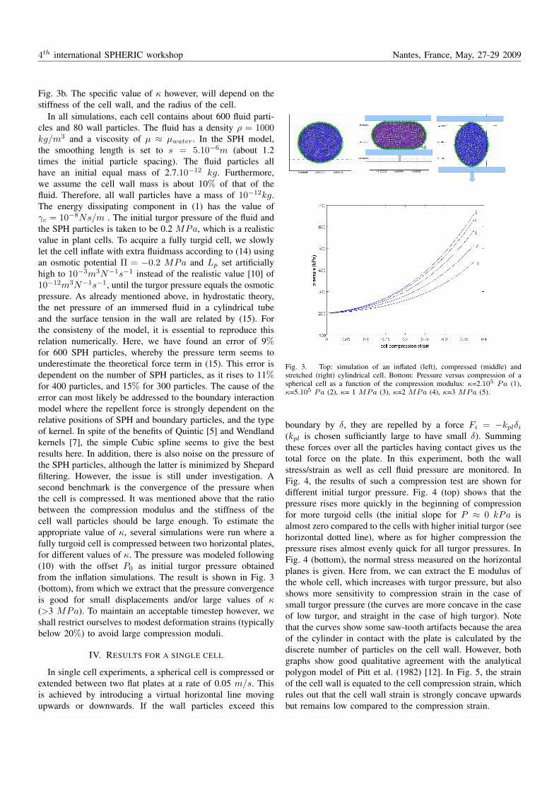
Fig. 3b. The specific value of κ however, will depend on thestiffness of the cell wall, and the radius of the cell.

In all simulations, each cell contains about 600 fluid parti-cles and 80 wall particles. The fluid has a density ρ = 1000kg/m3 and a viscosity of µ ≈ µwater. In the SPH model,the smoothing length is set to s = 5.10−6m (about 1.2times the initial particle spacing). The fluid particles allhave an initial equal mass of 2.7.10−12 kg. Furthermore,we assume the cell wall mass is about 10% of that of thefluid. Therefore, all wall particles have a mass of 10−12kg.The energy dissipating component in (1) has the value ofγc = 10−8Ns/m . The initial turgor pressure of the fluid andthe SPH particles is taken to be 0.2 MPa, which is a realisticvalue in plant cells. To acquire a fully turgid cell, we slowlylet the cell inflate with extra fluidmass according to (14) usingan osmotic potential Π = −0.2 MPa and Lp set artificiallyhigh to 10−3m3N−1s−1 instead of the realistic value [10] of10−12m3N−1s−1, until the turgor pressure equals the osmoticpressure. As already mentioned above, in hydrostatic theory,the net pressure of an immersed fluid in a cylindrical tubeand the surface tension in the wall are related by (15). Forthe consisteny of the model, it is essential to reproduce thisrelation numerically. Here, we have found an error of 9%for 600 SPH particles, whereby the pressure term seems tounderestimate the theoretical force term in (15). This error isdependent on the number of SPH particles, as it rises to 11%for 400 particles, and 15% for 300 particles. The cause of theerror can most likely be addressed to the boundary interactionmodel where the repellent force is strongly dependent on therelative positions of SPH and boundary particles, and the typeof kernel. In spite of the benefits of Quintic [5] and Wendlandkernels [7], the simple Cubic spline seems to give the bestresults here. In addition, there is also noise on the pressure ofthe SPH particles, although the latter is minimized by Shepardfiltering. However, the issue is still under investigation. Asecond benchmark is the convergence of the pressure whenthe cell is compressed. It was mentioned above that the ratiobetween the compression modulus and the stiffness of thecell wall particles should be large enough. To estimate theappropriate value of κ, several simulations were run where afully turgoid cell is compressed between two horizontal plates,for different values of κ. The pressure was modeled following(10) with the offset P0 as initial turgor pressure obtainedfrom the inflation simulations. The result is shown in Fig. 3(bottom), from which we extract that the pressure convergenceis good for small displacements and/or large values of κ(>3 MPa). To maintain an acceptable timestep however, weshall restrict ourselves to modest deformation strains (typicallybelow 20%) to avoid large compression moduli.

IV. RESULTS FOR A SINGLE CELL

In single cell experiments, a spherical cell is compressed orextended between two flat plates at a rate of 0.05 m/s. Thisis achieved by introducing a virtual horizontal line movingupwards or downwards. If the wall particles exceed this

Fig. 3. Top: simulation of an inflated (left), compressed (middle) andstretched (right) cylindrical cell. Bottom: Pressure versus compression of aspherical cell as a function of the compression modulus: κ=2.105 Pa (1),κ=5.105 Pa (2), κ= 1 MPa (3), κ=2 MPa (4), κ=3 MPa (5).

boundary by δ, they are repelled by a force Fi = −kplδi(kpl is chosen sufficiantly large to have small δ). Summingthese forces over all the particles having contact gives us thetotal force on the plate. In this experiment, both the wallstress/strain as well as cell fluid pressure are monitored. InFig. 4, the results of such a compression test are shown fordifferent initial turgor pressure. Fig. 4 (top) shows that thepressure rises more quickly in the beginning of compressionfor more turgoid cells (the initial slope for P ≈ 0 kPa isalmost zero compared to the cells with higher initial turgor (seehorizontal dotted line), where as for higher compression thepressure rises almost evenly quick for all turgor pressures. InFig. 4 (bottom), the normal stress measured on the horizontalplanes is given. Here from, we can extract the E modulus ofthe whole cell, which increases with turgor pressure, but alsoshows more sensitivity to compression strain in the case ofsmall turgor pressure (the curves are more concave in the caseof low turgor, and straight in the case of high turgor). Notethat the curves show some saw-tooth artifacts because the areaof the cylinder in contact with the plate is calculated by thediscrete number of particles on the cell wall. However, bothgraphs show good qualitative agreement with the analyticalpolygon model of Pitt et al. (1982) [12]. In Fig. 5, the strainof the cell wall is equated to the cell compression strain, whichrules out that the cell wall strain is strongly concave upwardsbut remains low compared to the compression strain.


(a)

(b)

Fig. 4. (a) Simulated relation between the cell fluid pressure for threedifferent inital turgor pressures during compression of a cylindrical cell (lines1-3), and the stretching of a cell (line 4). (b) Relation between the cellcompression strain and the plate - cell wall stress.

Fig. 5. Simulated relation between the cell strain and cell wall strain. Solidline: compression (1) ν = 0.5, (2) ν = 0. Dashed line: stretching.

In the tensile loading experiment, we fix one particle of thecell wall while the opposite particle is attached to an objectmoving with a constant velocity. In Fig. 4, the pressure curveis shown for this experiment (line 4), from which we extractthat the pressure only slightly increases with the strain (it even

bonded walls

x

y

Fig. 6. Simulation of a bonded aggregate of cells, small voids. Top: initialphase, down: inflated phase (turgid cells).

decreases for small strains). In the cell-wall strain experiment(Fig. 5), the wall strain shows a comparable behavior withrespect to the compression experiment, although the relationis much more linear here, especially for larger strains.

V. RESULTS FOR CELL AGGREGATES

A plant is not a homogeneous aggregate of undifferentiatedcells. Usually, it is a collection of tissue in which the cellshave a specific function. For example, the epidermis cellsmake the outer parts of the plant, whereas the pith tissueoccupies the large central part of the stem. In this paper, wefocus on the cortex tissue which is mainly composes of largestorage cells (parenchyma) that contain the fruit constituents.Inside this cortex, the structure is mainly built by cells andintercellular voids which can vary in size (in pears, the voidvolume fraction is around 5% while in apples this can go upto 23% [13]). It has been stated by several authors that themechanical properties of bulk tissue is dictated by the cellsthemselves, the intercellular air spaces, and the middle lamella.Yielding of tissue is generally addressed to the rupture of thecell walls and/or debonding of the cells.

Because the individual cell properties are already discussedin the previous section, we shall now focus on those whodetermine the structure of the tissue, namely the geometryof the cells, and the intercellular voids. Therefore, we startrepresenting the tissue by an aggregate of 10 individualrectangular cells which are initially positioned in a rectangularbrick pattern. Next, we consider two different geometricalstructures. In the first case, all cells are perfectly attachedto each other (no voids). In the second case, the cells are


Intracellular spaces

unbonded walls

x

ybonded wall

Fig. 7. Simulation of unbonded cells, large voids. Top: initial phase, down:inflated phase. To minimize the boundary effects at the edge of the aggregate,the length over which the forces are calulated is limited (indicated by thehorizontal grey arrows).

separated such that the intercellular spaces are substantial.The two case are represented in Fig. 6-7. Inflation of thecells is again established applying (13). Note that, as thecells are inflated, a remarkable difference can be observedbetween the two void fractions. If these are low, the aggregateresembles the typical honeycomb-like structure observed indensely packed cells (see also Fig. 1a). However, if the voidfraction is larger, the cell structure evolves to an aggregate of(almost) round cells. This structure is especially observed inapple cortex [13].

After inflation, the aggregate is compressed slowly (0.05m/s in Y direction) between two flat plates, as is shown inFig. 8 (top). The monitored stresses between the plates for thetwo different aggregate types are show in Fig. 9. The Youngmoduli derived from this simulations are around 2 MPa forthe compact tissue and about 1 MPa for the aggregate withvoids, comparable to what is found experimentally for appletissue in literature [14]. The appearant difference in the moduliis not surprising, since the presence of voids allow the cellsto expand, while in dense aggregate, the imcompressibility ofthe fluid plays a more dominant role. This is contrary to whatis observed in shear displacements simulations (displacementsare in X direction now), where the first results reveal that theshear moduli of both structures are almost equal. As a finalremark, we want to emphasize that the results must be treatedwith caution, because they are offset by boundary effectsinduced by the outer positioned cells. To account for this, onlythe forces in the middle section are considered (indicated bythe grey arrow is Fig. 6-7). Ideally however -not to mention

x

y

Fig. 8. Simulated compression a cell aggregate: (top) aggregate with largevoids, (down) large voids.

Fig. 9. Simulated stress-strain relation for a compression simulation of acell aggregate: (1) no intercellular voids, (2) large intercellular voids. Youngmoduli are deduced from the slopes of the curves.

real 3D models- one should perform simulations with morelayers in order to be comparable with real experiments.

VI. CONCLUSION

A micromechanical, cell based model for the simulation ofplant tissue has been presented. The model describes both thesolid phase (i.e. cell wall) and the cell fluid through a combina-tion of SPH and DEM. After checking the model consistency,simulations for rheological experiments on both single cellsand cell aggregates have been carried out, yielding goodqualitative agreement with other models, although extensive


comparison with experiments on real tissue is still mandatory.In the future, also dynamical (e.g. impact) problems will beaddressed where the cell fluid and cell wall viscosity will comeinto play. To account for cell debonding, wall-wall interactionmodels will have to be developped. Eventually, our aim isto model macroscale tissue engineering problems, such asbruising prediction and prevention, but also more fundamentalproblems in plant physiology, such as the relation betweenstress on the cellular level, the cell growth rate, modified geneexpression, defensive mechanisms and visible effects on theplant. Research on multi-scale coupling with Finite ElementMethods will therefore be eminent.

ACKNOWLEDGMENT

Research is conducted utilizing high performance compu-tational resources provided by the University of Leuven,http://ludit.kuleuven.be/hpc. The authors would also like tothank the OT (KUL). Giovanni Samaey is a Postdoctoral Fel-low of the Research Foundation - Flanders (FWO-Vlaanderen).

REFERENCES

[1] M. Van Zeebroeck, The discrete element method (DEM) to simulate fruitimpact damage during transport and handling, Phd thesis, KUleuven,Belgium, 2005.

[2] J. Loodts, E. Tijskens, W. Chunfang, E. Van Streels, B. Nicola ,H. Ramon,Micromechanics: simulating the elastic behaviour of onion epidermistissue. Journal of Texture Studies, (37), p16-34, 2006.

[3] P. Ghysels, G. Samaey, B. Tijskens, P. Van Liedekerke, H. Ramon and D.Roose, Multi-scale simulation of plant tissue deformation using a modelfor individual cell mechanics. Phys. Biol. (6), 2009.

[4] D.H. Boal. Mechanics of the Cell, New York, NY: Cambridge UniversityPress, 2002.

[5] J.P. Morris , P.J. Fox , Y.Z., Modeling low Reynolds number incom-pressible flows using SPH, Journal of Computational Physics, v.136 n.1,p.214-226, 1997.

[6] J.J. Monaghan, Simulating free surface flows with SPH, Journal ofComputational Physics, v.110 n.2, p.399-406, 1994.

[7] M. Robinson, J.J. Monaghan, Forced two-dimensional wall-boundedturbulence using SPH, 3th ERCOFTAC SPHERIC workshop on SPHsimulatons, June 4-6, Lausanne, Switzerland, 2008.

[8] H. Tekeda, S.M. Miyama, M.Sekiya, Numerical simulation of viscousflow by Smoothed Particle Hydrodynamics , Prog. theor. Phys., 92(5), p939, 1994.

[9] E. Tijskens, F Rioual, Representing particle shape in discrete elementmodeling. Relpowflo IV, 10-12 June 2008, Tromso, Norway, 2008.

[10] N. Wu , M.J Pitts, Development and validation of a finite element modelof an apple fruit cell, p. 1-8(8), 1999.

[11] L. taiz, E. Zeiger, Plant physiology, Sunderland, Massachussets, SinauerAssociates, 2002.

[12] R.E. Pitt, Models for the rheology and statistical strength of uniformlystressed vegetable tissue. Trans Am Soc Agric Eng, 25(6), p.17761784,1982.

[13] P. Verboven, G. Kerckhofs, H. K. Mebatsion, Q. T. Ho, K. Temst, M.Wevers, P. Cloetens and B. M. Nicola, Three-Dimensional Gas ExchangePathways in Pome Fruit Characterized by Synchrotron X-Ray ComputedTomography. Plant Physiology, 147, p518-527, 2008.

[14] N.N. Mohensin, Physical properties of plant and animal materials, NewYork, Gordon and Breach Science publishers, 1970.

[15] Hsin-I Wu, R. D. SPence, P.J.H. SHarpe, J. D. Goeschl, Cell wallelasticity: I. A critique of the bulk elastic modulus approach and ananalysis using polymer elastic. Plant, Cell & Environment, 8(8), P563- 570, 1985.

A particle based model to simulate plant cells dynamics

Documents

Transcript of A particle based model to simulate plant cells dynamics