Novel method for the isolation and characterisation of the putative prostatic stem cell
Upload
independentCategory
view
0download
0
ContributionstoPlasmaPhysicsCPP
www.cpp-journal.org
REPRINT
The Particle-In-Cell Method
D. Tskhakaya1,4, K. Matyash2, R. Schneider2, and F. Taccogna3
1 Association Euratom-OAW, Institute of Theoretical Physics, University of Innsbruck, A-6020 Innsbruck,Austria
2 Max-Planck-Institut fur Plasmaphysik, EURATOM Association, Wendelsteinstrasse 1, D-17491, Greifswald,Germany
3 Dipartimento di Chimica, Universita’ degli Studi di Bari and Istituto di Metodologie Inorganiche e di Plasmi- CNR, Sect. Bari, via Orabona 4, Bari, 70126, Italy
4 Permanent address: Institute of Physics, Georgian Academy of Sciences, 380076 Tbilisi, Georgia
Received 19 October 2007, accepted 5 November 2007Published online 14 December 2007
Key words PIC simulations, MC simulations.PACS 52.65.-y, 52.65.Rr
This paper is the first in a series of three papers to summarize the recent work of an European-wide collaborationwhich is ongoing since about one decade using Particle-in-Cell (PIC) methods in low temperature plasmaphysics. In the present first paper the main aspects of this computational technique will be presented. In thesecond paper, an overview of applications in low-temperature plasma modelling will be given, whereas the thirdpart will put emphasis on the specific results of modelling ion thrusters.
Contrib. Plasma Phys. 47, No. 8–9, 563–594 (2007) / DOI 10.1002/ctpp.200710072

Contrib. Plasma Phys. 47, No. 8-9, 563 – 594 (2007) / DOI 10.1002/ctpp.200710072
The Particle-In-Cell Method
D. Tskhakaya∗1,4, K. Matyash2, R. Schneider2, and F. Taccogna3
1 Association Euratom-OAW, Institute of Theoretical Physics, University of Innsbruck, A-6020 Innsbruck,Austria
2 Max-Planck-Institut fur Plasmaphysik, EURATOM Association, Wendelsteinstrasse 1, D-17491, Greifswald,Germany
3 Dipartimento di Chimica, Universita’ degli Studi di Bari and Istituto di Metodologie Inorganiche e di Plasmi- CNR, Sect. Bari, via Orabona 4, Bari, 70126, Italy
4 Permanent address: Institute of Physics, Georgian Academy of Sciences, 380076 Tbilisi, Georgia
Received 19 October 2007, accepted 5 November 2007Published online 14 December 2007
Key words PIC simulations, MC simulations.PACS 52.65.-y, 52.65.Rr
This paper is the first in a series of three papers to summarize the recent work of an European-wide collaborationwhich is ongoing since about one decade using Particle-in-Cell (PIC) methods in low temperature plasmaphysics. In the present first paper the main aspects of this computational technique will be presented. In thesecond paper, an overview of applications in low-temperature plasma modelling will be given, whereas the thirdpart will put emphasis on the specific results of modelling ion thrusters.
c© 2007 WILEY-VCH Verlag GmbH & Co. KGaA, Weinheim
1 Introduction
Particle-in-Cell (PIC) simulation represents a powerful tool for plasma studies having a number of advantages likethe fully kinetic description of high-dimensional plasma and the ability to incorporate complicated atomic andplasma-surface interactions. PIC simulations are used practically in all branches of laboratory and astrophysicalplasma physics. PIC era started in the late 1950s by Buneman [1] and Dawson [2] who simulated the motion of100–1000 particles including interactions between them. Our day PIC codes can simulate up to 1010 particlesand represent complicated numerical tools requiring high level of optimization. As a result the PIC codes areusually designed for a professional use.
The aim of the present paper is to introduce the reader to the basics of the PIC simulation technique. The paperis based on our previous work [3]. For the interested reader we can recommend two classical monographs, [4]and [5].
The paper is organized as follows. The main structure of the PIC algorithm is discussed in Sec. 2. In Sec. 3we consider solvers of equations of motion. We discuss the accuracy and stability aspects of these solvers.Initialization of particle distribution, boundary effects and particle sources are described in Sec. 4. In Secs. 5 and6 we show how plasma macro-parameters are calculated and discuss solvers of Maxwell’s equations. In Sec. 7we consider a linear theory of finite size particle plasmas. Different models of particle collisions are consideredin Sec. 8. Optimization of PIC codes and Grid-free methods are briefly considered in Sec. 10.
2 General scheme of PIC simulation
The PIC simulation is based on a trivial idea: The code simulates the motion of each plasma particle and calculatesall macro-quantities (like density, current density and so on) from the position and velocity of these particles. Themacro-force acting on the particles is calculated from the field equations. The name Particle-in-Cell comes from
∗Corresponding author: e-mail: [email protected]: +43 512 507 6225, Fax: +43 512 507 2919
c© 2007 WILEY-VCH Verlag GmbH & Co. KGaA, Weinheim

564 D. Tskhakaya et al.: The PIC method
the way of assigning macro-quantities to the simulation particles. In general, any numerical simulation model,which simultaneously solves the equations of motion of N particles,
d Xi
dt= Vi and
dVi
dt= Fi
(t, Xi, Vi, A
)(1)
for i = 1, . . . , N and of macro fields A = L1(B), with the prescribed rule of calculation of macro quantities B =L2
(X1, V1, . . . , XN , VN
)from the particle position and velocity can be called a PIC simulation. Here Xi and Vi
are the generalized (multi-dimensional) coordinate and velocity of the particle i. A and B are macro fields actingon particles and some macro-quantities associated with particles, respectively. L1 and L2 are some operators andFi is the force acting on a particle i. As one can see, PIC simulations have much broader applications then justplasma physics, like solid state or quantum physics. On the other hand, inside the plasma community PIC codesare usually associated with codes solving the equation of motion of particles with the Newton–Lorentz’s force(for simplicity we consider an unrelativistic case)
d Xi
dt= Vi and
dVi
dt=
ei
mi
(E(
Xi
)+ Vi × B
(Xi
))(2)
for i = 1, . . . , N and the Maxwell’s equations:
∇ D = ρ (r, t) ,∂ B
∂t= −∇× E , D = ε E ,
∇ B = 0 ,∂ D
∂t= ∇× H − J (r, t) , B = µ H ,
(3)
together with the prescribed rule of calculation of ρ and J
ρ = ρ(
X1, V1, . . . , XN , VN
), (4)
J = J(
X1, V1, . . . , XN , VN
). (5)
Here ρ and J are the charge and current densities and ε and µ the permittivity and permeability of the medium,respectively. Below we will follow this definition of the PIC codes.
PIC codes usually are classified depending on the dimensionality of the code and on the set of Maxwell’sequations used. The codes solving a whole set of Maxwell’s equations are called electromagnetic codes, contraryelectrostatic ones solve just the Poisson equation. The dimensionality of the PIC code is usually given as mDnV,where m and n define dimensionality in usual and velocity spaces, respectively. Some advanced codes are able toswitch between different dimensionality and coordinate system, and use electrostatic, or electro-magnetic models(e.g. the XOOPIC code [6]).
A simplified scheme of the PIC simulation is given in Fig. 1. PIC simulation starts with an initialization andends with the output of results. This part is similar to the input/output routines of any other numerical tool. Otherparts represent specific PIC routines, which we consider separately.
3 Integration of Equations of Particle Motion
3.1 Description of Particle Movers
During a PIC simulation the trajectory of all particles is followed, which requires the solution of the equations ofmotion for each of them. This part of the code is frequently called particle mover.
The number of particles in a real plasma is extremely large and exceeds by orders of magnitude the maximumpossible number of particles, which can be handled by the best supercomputers. Hence, during a PIC simulation itis usually assumed that one simulation particle consists of many physical particles. Because the ratio charge/massis invariant to this transformation, this superparticle follows the same trajectory as the corresponding plasmaparticle. As a result the plasma model simulated by a superpaticle is absolutely similar to a real one (assuming that
c© 2007 WILEY-VCH Verlag GmbH & Co. KGaA, Weinheim www.cpp-journal.org

Contrib. Plasma Phys. 47, No. 8-9 (2007) / www.cpp-journal.org 565
Input/Output
Solution of Maxwell’s
equations
Calculation of plasma
parameters (n, J,…)
Calculation of force
acting on particles Plasma source and
boundary effects
Integration of equations
of particle motionParticle collisions
Fig. 1 Scheme of the PIC simulation.
all necessary parameters are properly re-scaled). One has to note that for 1D and 2D models this transformationcan be easily avoided by choosing a sufficiently small simulated volume, so that the number of real plasmaparticles can be chosen arbitrary.
As we will see below, the number of simulated particles is defined by a set of physical and numerical restric-tions, and usually it is extremely large (> 105). As a result, the main requirements to the particle mover are highaccuracy and speed. One of such solvers represents the so called leap-frog method (see [4] and [5]), which wewill consider in detail.
As in other numerical codes the time in PIC is divided into discrete time steps, in other words the timeis gridded. This means that physical quantities are calculated only at given time steps. Usually, the intervalbetween the time steps ∆t, is constant, so that the simulated time can be given as: t → tk = t0 + k∆t andA (t) → Ak = A (t = tk) with k = 0, 1, 2, . . ., where t is the time, t0 the initial time and A denotes anyphysical quantity. The leap-frog method calculates particle velocities not at usual time steps tk, but betweenthem tk+1/2 = t0 + (k + 1/2)∆t. In this way equations become time-centered, so that they are sufficientlyaccurate and require relatively short calculation time:
Xk+1 − Xk
∆t= Vk+1/2 ,
Vk+1/2 − Vk−1/2
∆t=
e
m
(Ek +
Vk+1/2 + Vk−1/2
2× Bk
).
(6)
The leap-frog scheme is an explicit solver, i.e. it depends on old forces from the previous time step k. Contrary toimplicit schemes, when for calculation of particle velocity only quantities at the time step k + 1 are used, explicitsolvers are simpler and faster, but their stability requires a smaller time step ∆t.
Some remarks about the accuracy of this leap-frog solver. By substituting
Vk±1/2 = Vk ± ∆t
2V ′
k +∆t2
8V ′′
k ± 16
(∆t
2
)3
V ′′′k + . . . ,
Xk+1 = Xk + ∆tVk +∆t2
2V ′
k +∆t3
6V ′′
k + ...
(7)
into (6) we obtain the order of the error ∼ ∆t2. It satisfies a general requirement for the scaling of numericalaccuracy ∆ta>1. In order to understand this requirement we recall that for a fixed simulated time the number ofsimulated time steps scales as Nt ∼ ∆t−1. Then, after Nt time steps an accumulated total error will scale asNt∆ta ∼ ∆ta−1, where ∆ta is the scale of the error during one step. Thus, only a > 1 can guarantee, that theaccuracy increases with decreasing ∆t.
There exist different methods for solving finite-difference equations (6). Below we consider the Boris method(see [4]), which is frequently used in PIC codes:
Xk+1 = Xk + ∆tVk+1/2 and Vk+1/2 = u+ + q Ek , (8)
www.cpp-journal.org c© 2007 WILEY-VCH Verlag GmbH & Co. KGaA, Weinheim

566 D. Tskhakaya et al.: The PIC method
with u+ = u− + (u− + (u− ×h))×s, u− = Vk−1/2 + q Ek, h = q Bk, s = 2h/(1 + h2) and q = e∆t/2m. Al-though these equations look very simple, their solution represents the most time consuming part of PIC, becauseit is done for each particle separately. As a result, the optimization of the particle mover can significantly reducethe simulation time. One example for such an optimization is considered below.
In general, the Boris method requires 39 operations (18 adds and 21 multiplies), assuming that B is constantand h, s and q are calculated only once at the beginning of simulation. But if B has one or two non-zerocomponents, then the number of operations can be significantly reduced. E.g., if B ‖ z and E ‖ x then (8) canbe reduced to the following ones
Xk+1 = Xk + ∆tVk+1/2 ,
V xk+1/2 = ux
− +(V y
k+1/2 + V yk−1/2
)h + qEx
k ,
V yk+1/2 = V y
k−1/2 (1 − sh) − ux−s
(9)
with ux− = V xk−1/2 + qEx
k . They require just 17 operations (8 multiplies and 9 adds), which can save up to 50%of the CPU time. Some advanced PIC codes include a subroutine for searching the fastest solver for a givensimulation setup, which significantly decreases the CPU time (e.g. the BIT1 code [7]).
3.2 Accuracy and Stability of the Particle Mover
In order to find correct simulation parameters one has to know the absolute accuracy and corresponding stabilityconditions for the particle mover. They are different for different movers and the example considered below isapplied just to the Boris scheme.
First of all let us consider the accuracy of a Larmor rotation. By assuming Vk−1/2 ⊥ B we can define therotation angle during the time ∆t from the following expression:
cos (ω∆t) =Vk+1/2
Vk−1/2
V 2k−1/2
. (10)
On the other hand, substituting (8) into (10) we obtain
Vk+1/2Vk−1/2
V 2k−1/2
=1 − (∆tΩ)2
4
1 + (∆tΩ)2
4
(11)
with Ω = eB/m, so that for a small ∆t we get ω = Ω(1 − 1/12(∆tΩ)2) + . . .. E.g., for a 1% accuracy thefollowing condition has to be satisfied: ∆tΩ ≤ 0.35.
In order to formulate the general stability condition some complicated calculations are required (see [5]).Below we present simple estimates of the stability criteria for the (explicit) particle mover.
Let us consider the equation of a linear harmonic oscillator:
d2X
dt2= −ω2
0X , (12)
having the following analytic solution
X = Ae−iω0t , (13)
where A is an arbitrary imaginary number. The corresponding Leap-frog equations take the following form:
Xk+1 − 2Xk + Xk−1
∆t2= −ω2
0Xk . (14)
We assume that the solution has a form similar to (13), Xk = A exp (−iωtk). After substitution into (14) andperforming simple transformations we find
sin(
ω∆t
2
)= ±ω0∆t
2. (15)
c© 2007 WILEY-VCH Verlag GmbH & Co. KGaA, Weinheim www.cpp-journal.org
Contrib. Plasma Phys. 47, No. 8-9 (2007) / www.cpp-journal.org 567
Hence, for a stable solution Im(ω) ≤ 0 the condition
ω0∆t < 2 (16)
is required. Frequently during PIC simulations much more restrictive condition is used:
ω0∆t ≤ 0.2 , (17)
giving sufficiently accurate results. Interesting to note that this number has been derived few decades ago whenthe number of simulation time steps was typically of the order of Nt ∼ 104. From (15) we obtain ω = ω0(1 −1/24(ω0∆t)2) + . . .. Hence, a cumulative phase error after Nt steps should be ∆(ω∆t) ≈ (Nt(ω0∆t)3)/24.Assuming Nt = 104 and ∆ (ω∆t) < π we obtain the condition (17). Although modern simulations containmuch larger number of time steps up to Nt = 107, this condition still can work surprisingly well.
The restrictions on ∆t described above can require the simulation of unacceptably large number of time steps.In order to avoid these restrictions different implicit schemes have been introduced: Vk+1/2 = F ( Ek+1, ...). Thedifference from the explicit scheme is that for the calculation of the velocity only quantities at the new time stepare used.
One example of an implicit particle mover represents the so called 1 scheme (see [8])
Xk+1 − Xk
∆t= Vk+1/2 ,
Vk+1/2 − Vk−1/2
∆t=
e
m
(Ek+1(xk+1) + Ek−1
2+
+Vk+1/2 + Vk−1/2
2× Bk
).
(18)
It can be shown that for a harmonic oscillator (see (12))
V, X ∼ 1
(ω0∆t)2/3(19)
if ω0∆t 1. Hence, the corresponding oscillations are heavily damped and the solver (see (18)) can filterunwanted oscillations. As a result, the condition (16) can be neglected.
More rigorous stability analysis will be done in Sec. 7.
4 Plasma Source and Boundary Effects
4.1 Boundary Effects
From the physics point of view, the boundary conditions for the simulated particles are relatively easy to formu-late: Particles can be absorbed at boundaries, or injected from there with any distribution. On the other hand,an accurate numerical implementation of particle boundary conditions can be tricky. The problem is that (i) thevelocity and position of particles are shifted in time (∆t/2) and (ii) the velocity of particles are known at discretetime steps, while a particle can cross the boundary at any moment between these steps.
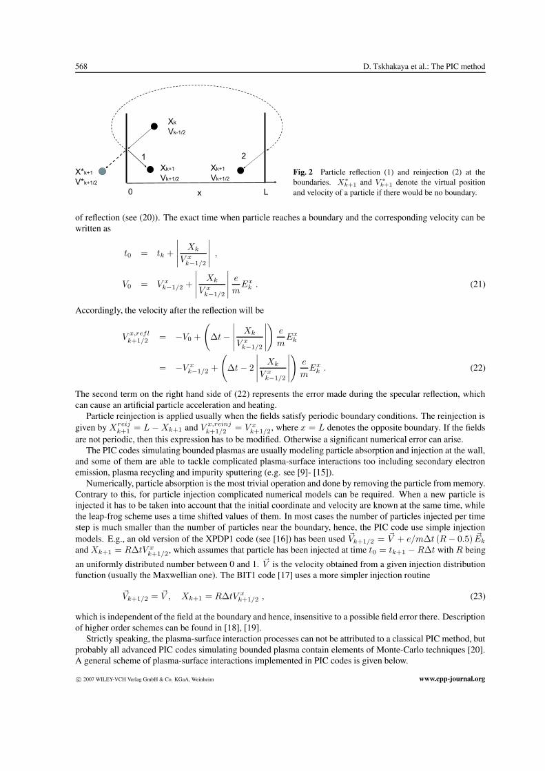
In unbounded plasma simulations particles are usually reflected at the boundaries, or reinjected from theopposite side (see Fig. 2).
A frequently used reflection model, so called specular reflection, is given as
Xreflk+1 = −Xk+1 and V x,refl
k+1/2 = −V xk+1/2 . (20)
Here, the boundary is assumed to be located at x = 0 (see Fig. 2). The specular reflection represents the simplestreflection model, but due to relatively low accuracy it can cause artificial effects. Let us estimate the accuracy
www.cpp-journal.org c© 2007 WILEY-VCH Verlag GmbH & Co. KGaA, Weinheim
568 D. Tskhakaya et al.: The PIC method
0 Lx
X*k+1
V*k+1/2
Xk+1
Vk+1/2
1 2
Xk+1
Vk+1/2
Xk
Vk-1/2
Fig. 2 Particle reflection (1) and reinjection (2) at theboundaries. X∗
k+1 and V ∗k+1 denote the virtual position
and velocity of a particle if there would be no boundary.
of reflection (see (20)). The exact time when particle reaches a boundary and the corresponding velocity can bewritten as
t0 = tk +
∣∣∣∣∣ Xk
V xk−1/2
∣∣∣∣∣ ,
V0 = V xk−1/2 +
∣∣∣∣∣ Xk
V xk−1/2
∣∣∣∣∣ e
mEx
k . (21)
Accordingly, the velocity after the reflection will be
V x,reflk+1/2 = −V0 +
(∆t −
∣∣∣∣∣ Xk
V xk−1/2
∣∣∣∣∣)
e
mEx
k
= −V xk−1/2 +
(∆t − 2
∣∣∣∣∣ Xk
V xk−1/2
∣∣∣∣∣)
e
mEx
k . (22)
The second term on the right hand side of (22) represents the error made during the specular reflection, whichcan cause an artificial particle acceleration and heating.
Particle reinjection is applied usually when the fields satisfy periodic boundary conditions. The reinjection isgiven by Xreij
k+1 = L − Xk+1 and V x,reinjk+1/2 = V x
k+1/2, where x = L denotes the opposite boundary. If the fieldsare not periodic, then this expression has to be modified. Otherwise a significant numerical error can arise.
The PIC codes simulating bounded plasmas are usually modeling particle absorption and injection at the wall,and some of them are able to tackle complicated plasma-surface interactions too including secondary electronemission, plasma recycling and impurity sputtering (e.g. see [9]- [15]).
Numerically, particle absorption is the most trivial operation and done by removing the particle from memory.Contrary to this, for particle injection complicated numerical models can be required. When a new particle isinjected it has to be taken into account that the initial coordinate and velocity are known at the same time, whilethe leap-frog scheme uses a time shifted values of them. In most cases the number of particles injected per timestep is much smaller than the number of particles near the boundary, hence, the PIC code use simple injectionmodels. E.g., an old version of the XPDP1 code (see [16]) has been used Vk+1/2 = V + e/m∆t (R − 0.5) Ek
and Xk+1 = R∆tV xk+1/2, which assumes that particle has been injected at time t0 = tk+1 − R∆t with R being
an uniformly distributed number between 0 and 1. V is the velocity obtained from a given injection distributionfunction (usually the Maxwellian one). The BIT1 code [17] uses a more simpler injection routine
Vk+1/2 = V , Xk+1 = R∆tV xk+1/2 , (23)
which is independent of the field at the boundary and hence, insensitive to a possible field error there. Descriptionof higher order schemes can be found in [18], [19].
Strictly speaking, the plasma-surface interaction processes can not be attributed to a classical PIC method, butprobably all advanced PIC codes simulating bounded plasma contain elements of Monte-Carlo techniques [20].A general scheme of plasma-surface interactions implemented in PIC codes is given below.
c© 2007 WILEY-VCH Verlag GmbH & Co. KGaA, Weinheim www.cpp-journal.org
Contrib. Plasma Phys. 47, No. 8-9 (2007) / www.cpp-journal.org 569
When a primary particle is absorbed at the wall, it can cause the emission of a secondary particle (a specialcase is reflection of the same particle). In general the emission probability F depends on the surface propertiesand primary particle energy ε and incidence angle α. Accordingly, the PIC code calculates F (ε, α) and comparesit to a random number R, uniformly distributed between 0 and 1. If F > R then a secondary particle is injected.The velocity of a secondary particle is calculated according to a prescribed distribution fsec
(V)
. Some codesallow multiple secondary particle injection, including as a special case the thermal emission. The functions Fand fsec are determined by surface and solid state physics.
4.2 Particle Loading
The particles in a PIC simulation appear, either by initial loading, or via particle injection from the boundary orfrom a volumetric source. In any case the corresponding velocities have to be calculated from a given distributionfunction f
(V)
. Important to note, that there is a significant difference between volumetric particle loading and
particle injection from the wall. In the first case the particle velocity is calculated directly from f(
V)
. Contrary
to this, the velocity of particles injected from the wall has to be calculated according to V xf(
V)
, where V x isthe component of the velocity normal to the wall. This becomes clear if we recall that the injection distributionfunction is the probability that particles having a distribution f
(V)
will cross the boundary with a given velocity
V . For simplicity we do not distinguish below these two functions denoting them f(
V)
.There exist two possibilities of calculation of velocities according to a given distribution. The most effective
way for a 1D case is to use a cumulative distribution function:
F (V ) =
V∫Vmin
f (V ′) dV ′
Vmax∫Vmin
f (V ′) dV ′(24)
with F (Vmin) = 0 and F (Vmax) = 1, representing a probability that the velocity of particle is between Vmin
and V . By equating this function to a sequence of uniformly distributed numbers U (or to random numbers R)between 0 and 1 and inverting it, we produce a sequence of V with the distribution f (V ) [4]:
F−1 (U) = V . (25)
The same method can be applied to multi-dimensional cases which can be effectively reduced to 1D, e.g., by vari-able separation: f
(V)
= f1 (V x) f2 (V y) f3 (V z). Often inversion of (25) can be done analytically, otherwiseit is done numerically.
As an example we consider the injection of Maxwell-distributed particles: f(V ) ∼ V exp(−V 2/(2V 2T )).
According to (24) and (25) we get
F (V ) = 1 − exp(− V 2
2V 2T
)and V = VT
√−2 ln (1 − U) . (26)
Another possibility is to use two sets of random numbers R1 and R2 (for simplicity we consider 1D case) ina von-Neumann rejection algorithm: V = Vmin + R1(Vmax − Vmin), if f (V ) /(fmax) > R2 use V , else tryonce more. This method requires random number generators of high level and it is time consuming. As a result,it is usually used when the method considered above can not be applied (e.g. for complicated multidimensionalf(
V)
).In advanced codes these distributions are generated and saved at the beginning of a simulation, so that later
no further calculations are required except getting V from the memory. The same methods are used for spatialdistributions f
(X)
, too.
www.cpp-journal.org c© 2007 WILEY-VCH Verlag GmbH & Co. KGaA, Weinheim

570 D. Tskhakaya et al.: The PIC method
x∆∆x 02/x∆2/x∆ 0
a)
b)
2/x∆2/x∆ 0
2/y∆
2/y∆0
2/x∆2/x∆ 0
2/y∆
2/y∆0
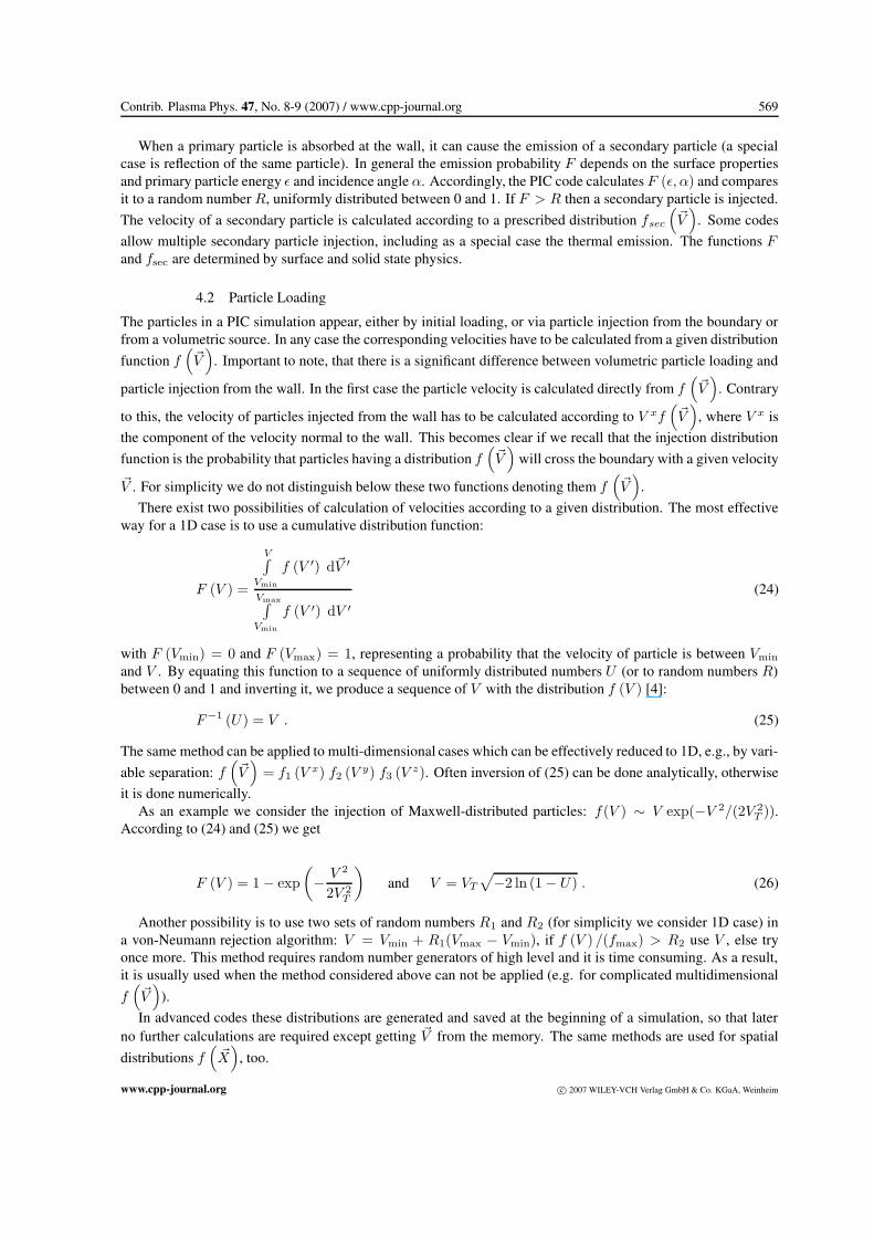
Fig. 3 Particle shapes for the NGP (left) and linear (right)weightings in 1D (a) and 2D (b) cases.
As it was mentioned above, required velocity distributions can be generated by a set of either ordered numbersU or by random numbers R, which are uniformly distributed between 0 and 1. A proper choice of these numbersis not a trivial task and depends on the simulated system; e.g., using random numbers can cause some noise.In addition, numerically generated random numbers in reality represent pseudo-random numbers, which cancorrelate and cause some unwanted effects. Contrary to this, the distributions generated by a set of orderednumbers, e.g. U = (i + 0.5) /N , i = 1, . . . , N − 1, are less noisy. On the other hand, in this case the generateddistributions represent a multi-beam distribution, which sometimes can cause a beam instability [4].
5 Calculation of Plasma Parameters and Fields Acting on Particles
5.1 Particle Weighting
All numerical schemes considered up to now can be applied not only to PIC, but to any test particle simulationtoo. In order to simulate a real plasma one has to self-consistently obtain the force acting on particles, i.e. tocalculate particle and current densities and solve Maxwell’s equations. The part of the code calculating macroquantities associated with particles (n, J , . . . ) is called particle weighting.
For a numerical solution of field equations it is necessary to grid the space: x → xi with i = 0, . . . , Ng.Here x is a general 3D coordinate and Ng number of grid cells (e.g. for 3D Cartesian coordinates Ng =(Nx
g , Nyg , Nz
g
)). Accordingly, the plasma parameters have to be known at these grid points: A(x) → Ai =
A(x = xi). The number of simulation particles at grid points is relatively low, so that one can not use an analyticapproach of point particles, which is valid only when the number of these particles is very large. The solutionis to associate macro parameters to each of the simulation particle. In other words to assume that particles havesome shape S
(x − X
), where X and x denote the particle position and observation point. Accordingly, the
distribution moments at the grid pointi associated with the particle “j” can be defined as
Ami
= amj S(xi − Xj
), (27)
where A0i
= ni, A1i
= niVi, A2
i= niV
2i
etc. and a0j = 1/Vg, a1
j = V j/Vg , a2j = (V j)2/Vg etc. Vg is the
volume occupied by the grid cell. The total distribution moments at a given grid point are expressed as
Ami
=N∑
j=1
amj S(xi − Xj
). (28)
Stability and simulation speed of PIC simulations strongly depend on the choice of the shape function S (x).It has to satisfy a number of conditions. The first two conditions correspond to space isotropy,
S (x) = S (−x) , (29)
c© 2007 WILEY-VCH Verlag GmbH & Co. KGaA, Weinheim www.cpp-journal.org
Contrib. Plasma Phys. 47, No. 8-9 (2007) / www.cpp-journal.org 571
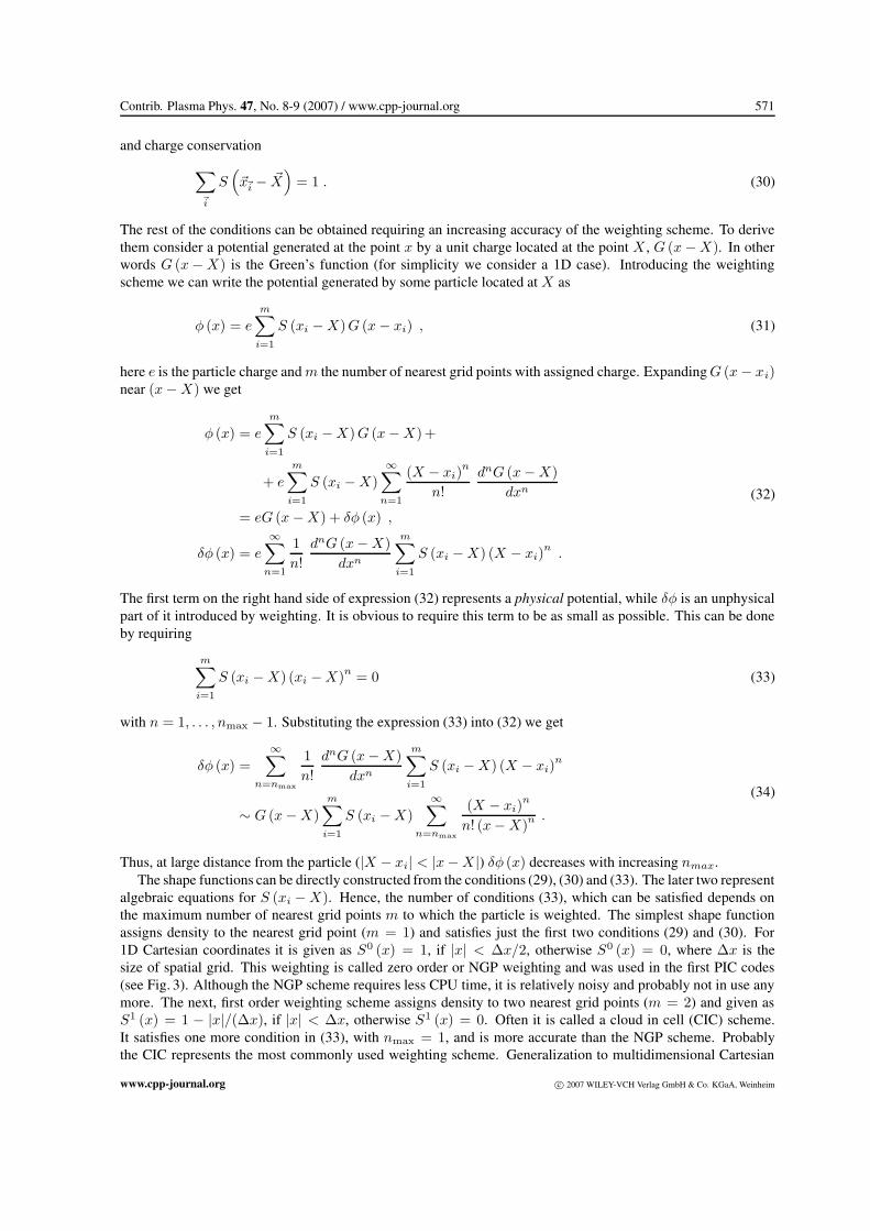
and charge conservation∑i
S(xi − X
)= 1 . (30)
The rest of the conditions can be obtained requiring an increasing accuracy of the weighting scheme. To derivethem consider a potential generated at the point x by a unit charge located at the point X , G (x − X). In otherwords G (x − X) is the Green’s function (for simplicity we consider a 1D case). Introducing the weightingscheme we can write the potential generated by some particle located at X as
φ (x) = em∑
i=1
S (xi − X)G (x − xi) , (31)
here e is the particle charge and m the number of nearest grid points with assigned charge. Expanding G (x − xi)near (x − X) we get
φ (x) = em∑
i=1
S (xi − X)G (x − X)+
+ e
m∑i=1
S (xi − X)∞∑
n=1
(X − xi)n
n!dnG (x − X)
dxn
= eG (x − X) + δφ (x) ,
δφ (x) = e
∞∑n=1
1n!
dnG (x − X)dxn
m∑i=1
S (xi − X) (X − xi)n
.
(32)
The first term on the right hand side of expression (32) represents a physical potential, while δφ is an unphysicalpart of it introduced by weighting. It is obvious to require this term to be as small as possible. This can be doneby requiring
m∑i=1
S (xi − X) (xi − X)n = 0 (33)
with n = 1, . . . , nmax − 1. Substituting the expression (33) into (32) we get
δφ (x) =∞∑
n=nmax
1n!
dnG (x − X)dxn
m∑i=1
S (xi − X) (X − xi)n
∼ G (x − X)m∑
i=1
S (xi − X)∞∑
n=nmax
(X − xi)n
n! (x − X)n .
(34)
Thus, at large distance from the particle (|X − xi| < |x − X |) δφ (x) decreases with increasing nmax.The shape functions can be directly constructed from the conditions (29), (30) and (33). The later two represent
algebraic equations for S (xi − X). Hence, the number of conditions (33), which can be satisfied depends onthe maximum number of nearest grid points m to which the particle is weighted. The simplest shape functionassigns density to the nearest grid point (m = 1) and satisfies just the first two conditions (29) and (30). For1D Cartesian coordinates it is given as S0 (x) = 1, if |x| < ∆x/2, otherwise S0 (x) = 0, where ∆x is thesize of spatial grid. This weighting is called zero order or NGP weighting and was used in the first PIC codes(see Fig. 3). Although the NGP scheme requires less CPU time, it is relatively noisy and probably not in use anymore. The next, first order weighting scheme assigns density to two nearest grid points (m = 2) and given asS1 (x) = 1 − |x|/(∆x), if |x| < ∆x, otherwise S1 (x) = 0. Often it is called a cloud in cell (CIC) scheme.It satisfies one more condition in (33), with nmax = 1, and is more accurate than the NGP scheme. Probablythe CIC represents the most commonly used weighting scheme. Generalization to multidimensional Cartesian
www.cpp-journal.org c© 2007 WILEY-VCH Verlag GmbH & Co. KGaA, Weinheim
572 D. Tskhakaya et al.: The PIC method
coordinates is trivial: S (x) = S (x) S (y)S (z). The higher order schemes (see [5]) can increase the accuracy ofsimulation (when other parameters are fixed), but require significantly longer CPU time.
Some authors often use another definition of the particle shape D (x) (e.g. see [5]):
S (xi − x) =
xi+∆x/2∫xi−∆x/2
D (x′ − x) dx′ . (35)
The meaning of this expression is that the density at the grid point xi assigned by the particle located at the pointx represents the average of the particle real shape D (x′ − x) over the area [xi − ∆x/2; xi + ∆x/2] . For thenearest grid point and linear weightings D (x) = δ (x) and D (x) = H (∆x/2 − |x|), respectively. Here H (x)is the step-function: H (x) = 1, if x > 0, else H (x) = 0.
The described method can be generalized for curvilinear coordinates, e.g. see [4], [6], [21] and referencesthere. Here we just note that this generalization is not straightforward and has to be done with a care, otherwiseweighting will not conserve the charge and current densities ( [21]- [23]).
5.2 Field Weighting
After the calculation of charge and current densities the code solves the Maxwell’s equations (cf. Fig. 1) anddelivers fields at the grid pointsi = 0, . . . , Ng . These fields can not be used directly for the calculation of forceacting on particles, which are located at any point and not necessarily at the grid points. Calculation of fields atany point is done in a similar way as charge assignment and called field weighting. So, we have Ei and Bi andwant to calculate E (x) and B (x) at any point x. This interpolation should conserve momentum, which can bedone by requiring that the following conditions are satisfied:
(i) Weighting schemes for the field and particles are same:
E (x) =∑i
EiS(xi − x
). (36)
(ii) The field solver has a correct spatial symmetry, i.e. formally the field can be expressed in the followingform (for simplicity we consider the 1D case):
Ei =∑
k
gikρk, gik = −gki, (37)
where ρk is the charge density at the grid point k. In order to understand this condition better, let us consider a1D electrostatic system. By integrating the Poisson equation we obtain:
E (x) =1
2ε0
⎛⎝ x∫a
ρ dx −b∫
x
ρ dx
⎞⎠+ Eb + Ea , (38)
where a and b define boundaries of the system. Assuming that either a and b are sufficiently far and Ea,b =ρa,b = 0, or the system (potential) is periodic Eb = −Ea, ρb = ρa, we obtain
E (xi) =1
2ε0
⎛⎝ xi∫a
ρ dx −b∫
xi
ρ dx
⎞⎠=
∆x
4ε0
⎛⎝i−1∑k=1
(ρk + ρk+1) −Ng−1∑k=i
(ρk + ρk+1)
⎞⎠ =
=∆x
4ε0
Ng∑k=1
gikρk
(39)
c© 2007 WILEY-VCH Verlag GmbH & Co. KGaA, Weinheim www.cpp-journal.org

Contrib. Plasma Phys. 47, No. 8-9 (2007) / www.cpp-journal.org 573
with Ng → ∞, ∆x = [b, a]/Ng and
gik =
⎧⎨⎩2 if i > k−2 if i < k0 if i = k
. (40)
Thus, the condition (37) is satisfied.Let us check different conservation constraints.
1. The self-force of the particle located at the point x can be calculated as follows:
Fself = e∑
i
EiS (xi − x) = e∑i, k
gikS (xi − x) ρk
=e2
Vg
∑i, k
gikS (xi − x)S (xi − x) = (i ↔ k)
= − e2
Vg
∑i, k
gikS (xi − x) S (xi − x) = −Fself = 0 ,
(41)
2. The two-particle interaction force is given as:
F12 = e1E2 (x1) = e1
∑i
E2,iS (xi − x1)
=e1e2
Vg
∑i, k
gikS (xi − x1) S (xk − x2)
= −e1e2
Vg
∑i, k
gkiS (xi − x1)S (xk − x2)
= −e2
∑i, k
gkiS (xk − x2) ρ1,k = −e2E1 (x2)
= −F21 .
(42)
Here, Ep denotes the electric field generated by the particle p.
Momentum conservation:
dP
dt= F =
N∑p=1
ep
(E (xp) + Vp × B (xp)
)
=N∑
p=1
ep
∑i
EiS (xi − xp) +N∑
p=1
epVp ×
∑i
BiS (xi − xp)
=∑
i
Ei
N∑p=1
epS (xi − xp) −∑i
Bi ×N∑
p=1
epVpS (xi − xp)
= Vg
∑i
(ρi
Ei + Ji × Bi
).
(43)
Representing fields as a sum of external and internal components Ei = Eexti
+ Einti
and Bi = Bexti
, whereEinti
is given in expression (36), after some trivial transformations we finally obtain the equation of momentumconservation
dP
dt= Vg
∑i
(ρi
Eexti
+ Ji × Bi
). (44)
www.cpp-journal.org c© 2007 WILEY-VCH Verlag GmbH & Co. KGaA, Weinheim
574 D. Tskhakaya et al.: The PIC method
As we see, the conditions (36) and (37) guarantee that during the force weighting the momentum is conservedand the inter-particle forces are calculated in a proper way. It has to be noted that:
1. We neglected contribution of an internal magnetic field Bint;
2. The momentum conserving schemes considered above does not necessarily conserve the energy too (forenergy conserving schemes see [4] and [5]);
3. The condition (37) is not satisfied in general for coordinate systems with nonuniform grids, causing theself-force and incorrect inter-particle forces. E.g., if we introduce a nonuniform grid ∆xi = ∆xαi withαi = αj =i, in expression (39) we obtain
E (xi) =∆x
4ε0
Ng∑k=1
gikρk , (45)
with
gik =
⎧⎪⎨⎪⎩αk + αk−1 if i > k
− (αk + αk−1)
if i < k, Ng → ∞, ∆x = [b,a]PNg
i=1 αi
αi−1 − αi if i = k
,
so that gki = −gik.
6 Solution of Maxwell’s Equations
6.1 General Remarks
Numerical solution of Maxwell’s equations is a continuously developing independent direction in numericalplasma physics (e.g., see [24]). Field solvers in general can be divided into three groups:
1. Mesh-relaxation methods, when the solution is initially guessed and then systematically adjusted until thesolution is obtained with required accuracy;
2. Matrix methods, when Maxwell’s equations are reduced to a set of linear finite difference equations andsolved by some matrix method, and
3. Methods using the so called fast Fourier transform (FFT) and solving equations in Fourier space.
According to the type of the equations to be solved the field solvers can be explicit or implicit. E.g., theexplicit solver of the Poisson equation solves the usual Poisson equation
∇ [ε (x)∇ϕ (x, t)] = −ρ (x, t) , (46)
while an implicit one solves the following equation:
∇ [(1 + η (x)) ε (x)ϕ (x, t)] = −ρ (x, t) . (47)
Here η (x) is the implicit numerical factor, which arises due to the fact that in its implicit formulation a newposition (and hence ρ) of particle is calculated from a new field given at the same moment.
As an example we consider some matrix methods, which are frequently used in different codes. For a generaloverview of different solvers the interested reader can see [4], [5], [25].
c© 2007 WILEY-VCH Verlag GmbH & Co. KGaA, Weinheim www.cpp-journal.org
Contrib. Plasma Phys. 47, No. 8-9 (2007) / www.cpp-journal.org 575
6.2 Electrostatic Case, Solution of Poisson Equation
Let us consider the Poisson equation in a Cartesian coordinate system(∂2
∂x2+
∂2
∂y2+
∂2
∂z2
)ϕ (r) = − 1
ε0ρ (r) , (48)
and formulate the corresponding finite difference equations. For this we use the transformation
∂2
∂x2ϕ ⇒ aϕi+1 + bϕi + cϕi−1
∆x2. (49)
Other components are treated in a similar way. Our aim is to choose the constants a, b and c, so that the error willbe smallest. From the symmetry constraint we can write a = c. Then by expanding ϕi±1 at x = xi
ϕi±1 = ϕi ± ∆x (ϕi)′ +
∆x2
2(ϕi)
′′ ± ∆x3
6(ϕi)
′′′ +∆x4
24(ϕi)
(4). . . ,
(ϕi)(k) =
(∂k
∂xkϕ
)x=xi
,
(50)
and substituting in (49) we obtain
aϕi+1 + bϕi + cϕi−1 = ϕi (2a + b) + (ϕi)′′
a∆x2 + (ϕi)(4)
a∆x4
12+ . . . . (51)
Hence, by choosing a = 1 and b = −2a = −2 we get(∂2ϕ
∂x2
)x=xi
− ϕi+1 − 2ϕi + ϕi−1
∆x2=
∆x2
12(ϕi)
(4) + Θ(∆x4)
. (52)
Hence, the finite difference equation (49) with b = −2 and a = c = 1 has second order accuracy (∼ ∆x2).Usually this accuracy is sufficient, otherwise one can consider a more accurate scheme
∂2
∂x2ϕ ⇒ aϕi+2 + bϕi+1 + cϕi + dϕi−1 + eϕi−2
∆x2. (53)
The x component of the electric field is calculated according to the following expression
Ei = −ϕi+1 − ϕi−1
2∆x(54)
Generalisation to the curvilinear coordinates is straightforward (see [4]).
6.2.1 1D Case: Bounded Plasma with External Circuit
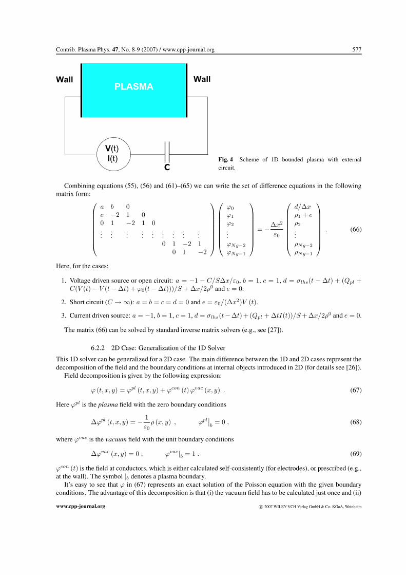
An excellent example of an 1D Poisson solver has been introduced in [16]. The solver is applied to an 1Dbounded plasma between two electrodes and solves Poisson and external circuit equations simultaneously. Later,this solver has been applied to a 2D plasma model [26]. Below we consider an simplified version of this solverassuming that the external circuit consists of a voltage (or current) source V (t) (I(t)) and a capacitor C (seeFig. 4)).
The Poisson equation for a 1D plasma is given as
ϕi+1 − 2ϕi + ϕi−1 = −∆x2
ε0ρi . (55)
This equation is second order, so that we need two boundary conditions for the solution. The first one can be apotential at the right-hand-side (rhs) wall:
ϕNg = 0. (56)
www.cpp-journal.org c© 2007 WILEY-VCH Verlag GmbH & Co. KGaA, Weinheim

576 D. Tskhakaya et al.: The PIC method
The second condition can be formulated at the left-hand-side (lhs) wall:
ϕ0 − ϕ1
∆x= E
(x =
∆x
2
)= E0 +
1ε0
∆x/2∫0
ρ dx ≈ E0 +∆x
2ε0ρ0 . (57)
Recalling that E0 is the electric field at the lhs wall, we can write E0 = σlhs/ε0, where σlhs is the surface chargedensity there. Hence, the second boundary condition can be formulated as
ϕ0 − ϕ1 =∆x
ε0
(σlhs +
∆x
2ρ0
). (58)
In order to calculate σlhs we have to employ the circuit equation.
Voltage Driven Source with Finite C In this case charge conservation at the lhs wall can be written as
σlhs (t) = σlhs (t − ∆t) +Qpl + Qci
S, (59)
where Qpl and Qci are the charge deposited during ∆t time on the lhs wall by the plasma and the external circuit,respectively. S is the area of the wall surface. Qpl can be calculated by counting the charge of the plasma particlesabsorbed at the lhs wall, and Qci can be given as Qci = Qc (t) − Qc (t − ∆t), where Qc is the charge at thecapacitor. Qc can be calculated using the Kirchhoff’s law
Qc
C= V (t) + ϕNg − ϕ0 = V (t) − ϕ0 . (60)
Substituting the expressions (59) and (60) into (58) we obtain
ϕ0
(1 +
C
S
∆x
ε0
)− ϕ1
=∆x
ε0
(Qpl + C (V (t) − V (t − ∆t) + ϕ0 (t − ∆t))
S+
+ σlhs (t − ∆t) +∆x
2ρ0
).
(61)
Voltage Driven Source with C → ∞ In this case in spite of (58) we use
ϕ0 − ϕNg = ϕ0 = V (t) . (62)
Open Circuit (C = 0) In this case we write
σlhs (t) = σlhs (t − ∆t) +Qpl
S, (63)
so that the second boundary condition takes the following form
ϕ0 − ϕ1 =∆x
ε0
(σlhs (t − ∆t) +
Qpl
S+
∆x
2ρ0
). (64)
Current Driven Source In this case Qci can be directly calculate from the expression Qci = ∆tI(t). Then thesecond boundary condition can be given as
ϕ0 − ϕ1 =∆x
ε0
(σlhs (t − ∆t) +
Qpl + ∆tI (t)S
+∆x
2ρ0
). (65)
c© 2007 WILEY-VCH Verlag GmbH & Co. KGaA, Weinheim www.cpp-journal.org
Contrib. Plasma Phys. 47, No. 8-9 (2007) / www.cpp-journal.org 577
PLASMA
V(t)
I(t)C
WallWall
Fig. 4 Scheme of 1D bounded plasma with externalcircuit.
Combining equations (55), (56) and (61)–(65) we can write the set of difference equations in the followingmatrix form:⎛⎜⎜⎜⎜⎜⎜⎜⎝
a b 0c −2 1 00 1 −2 1 0...
......
......
......
......
0 1 −2 10 1 −2
⎞⎟⎟⎟⎟⎟⎟⎟⎠
⎛⎜⎜⎜⎜⎜⎜⎜⎝
ϕ0
ϕ1
ϕ2
...ϕNg−2
ϕNg−1
⎞⎟⎟⎟⎟⎟⎟⎟⎠= −∆x2
ε0
⎛⎜⎜⎜⎜⎜⎜⎜⎝
d/∆xρ1 + eρ2
...ρNg−2
ρNg−1
⎞⎟⎟⎟⎟⎟⎟⎟⎠. (66)
Here, for the cases:
1. Voltage driven source or open circuit: a = −1 − C/S∆x/ε0, b = 1, c = 1, d = σlhs(t − ∆t) + (Qpl +C(V (t) − V (t − ∆t) + ϕ0(t − ∆t)))/S + ∆x/2ρ0 and e = 0.
2. Short circuit (C → ∞): a = b = c = d = 0 and e = ε0/(∆x2)V (t).
3. Current driven source: a = −1, b = 1, c = 1, d = σlhs(t−∆t)+ (Qpl + ∆tI(t))/S +∆x/2ρ0 and e = 0.
The matrix (66) can be solved by standard inverse matrix solvers (e.g., see [27]).
6.2.2 2D Case: Generalization of the 1D Solver
This 1D solver can be generalized for a 2D case. The main difference between the 1D and 2D cases represent thedecomposition of the field and the boundary conditions at internal objects introduced in 2D (for details see [26]).
Field decomposition is given by the following expression:
ϕ (t, x, y) = ϕpl (t, x, y) + ϕcon (t)ϕvac (x, y) . (67)
Here ϕpl is the plasma field with the zero boundary conditions
∆ϕpl (t, x, y) = − 1ε0
ρ (x, y) , ϕpl∣∣b
= 0 , (68)
where ϕvac is the vacuum field with the unit boundary conditions
∆ϕvac (x, y) = 0 , ϕvac|b = 1 . (69)
ϕcon (t) is the field at conductors, which is either calculated self-consistently (for electrodes), or prescribed (e.g.,at the wall). The symbol |b denotes a plasma boundary.
It’s easy to see that ϕ in (67) represents an exact solution of the Poisson equation with the given boundaryconditions. The advantage of this decomposition is that (i) the vacuum field has to be calculated just once and (ii)
www.cpp-journal.org c© 2007 WILEY-VCH Verlag GmbH & Co. KGaA, Weinheim
578 D. Tskhakaya et al.: The PIC method
the Poisson equation (68) with the zero boundary conditions is easier to solve, than one with a general boundaryconditions. As a result, the field decomposition can save a lot of CPU time.
The equation of the plasma field (68) is reduced to a set of finite difference equations
ϕi+1,j − 2ϕij + ϕi−1,j
∆x2+
ϕi,j+1 − 2ϕij + ϕi,j−1
∆y2= − 1
ε0ρij (70)
with ϕ|b = 0, which can be solved by matrix method. In a similar way the Laplace equation (69) can be solvedfor the vacuum field.
The corresponding boundary conditions at the wall of internal objects are calculated using Gauss’ law:∮ε E dS =
∫ρ dV +
∮σ dS , (71)
which in a finite volume representation can be written as
∆y∆z(εi+1/2,jEi+1/2,j − εi−1/2,jEi−1/2,j
)+
+ ∆x∆z(εi,j+1/2Ei,j+1/2 − εi,j−1/2Ei,j−1/2
)= ρij∆Vij + σij∆Sij .
(72)
Here ∆Vij and ∆Sij are the volume and area associated with the given grid point i, j. The electric fields enteringin this equation are calculated according to the following expressions
Ei±1/2,j = ±ϕi,j − ϕi±1,j
∆x, Ei,j±1/2 = ±ϕi,j − ϕi,j±1
∆x. (73)
Calculation of the potential at the plasma boundary ϕcon (t) consists in general of three parts. The potential atthe outer wall is fixed and usually chosen as 0. The potential at the electrodes, which are connected to an externalcircuit is done in a similar way as for the 1D case considered above. For calculation of the potential at the internalobject equation (72) is solved. We note that the later task is case dependent and not a trivial one, e.g., the solutiondepends on the object shape or material (conductor or dielectric). For further details see [26].
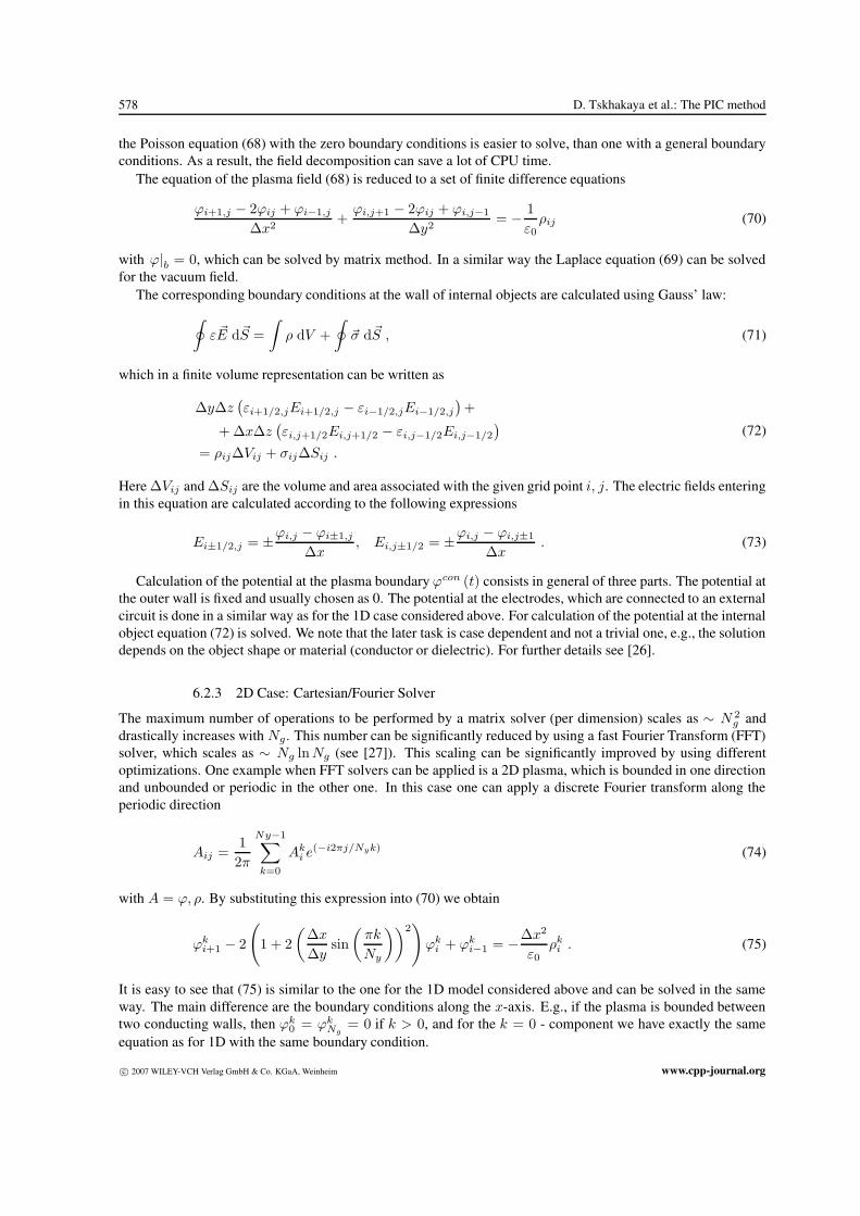
6.2.3 2D Case: Cartesian/Fourier Solver
The maximum number of operations to be performed by a matrix solver (per dimension) scales as ∼ N 2g and
drastically increases with Ng . This number can be significantly reduced by using a fast Fourier Transform (FFT)solver, which scales as ∼ Ng ln Ng (see [27]). This scaling can be significantly improved by using differentoptimizations. One example when FFT solvers can be applied is a 2D plasma, which is bounded in one directionand unbounded or periodic in the other one. In this case one can apply a discrete Fourier transform along theperiodic direction
Aij =12π
Ny−1∑k=0
Aki e(−i2πj/Nyk) (74)
with A = ϕ, ρ. By substituting this expression into (70) we obtain
ϕki+1 − 2
(1 + 2
(∆x
∆ysin(
πk
Ny
))2)
ϕki + ϕk
i−1 = −∆x2
ε0ρk
i . (75)
It is easy to see that (75) is similar to the one for the 1D model considered above and can be solved in the sameway. The main difference are the boundary conditions along the x-axis. E.g., if the plasma is bounded betweentwo conducting walls, then ϕk
0 = ϕkNg
= 0 if k > 0, and for the k = 0 - component we have exactly the sameequation as for 1D with the same boundary condition.
c© 2007 WILEY-VCH Verlag GmbH & Co. KGaA, Weinheim www.cpp-journal.org

Contrib. Plasma Phys. 47, No. 8-9 (2007) / www.cpp-journal.org 579
6.3 Electromagnetic Case
For sufficiently strong fields and/or very fast processes it is necessary to solve the complete set of Maxwell’sequations (3). It is obvious that corresponding solvers are more complicated than ones considered above. Corre-spondingly a detailed description of them is out of the scope of this work. Here we present just one of possibleschemes, which is implemented in the XOOPIC code [6].
In order to ensure high speed and accuracy it is convenient to introduce a leap-frog scheme also for the fields.The leap-frog scheme is applied to the space coordinates too, which means that electric and magnetic fields areshifted in time by ∆t/2, and different components of them are shifted in space by ∆x/2. In other words
1. E is defined at t = n∆t and B and J at t = (n + 1/2)∆t;
2. “i” components of the electric field and current density are defined at the points xi + ∆i/2, xk and xj , andsame component of the magnetic field at xi, xk + ∆k/2 and xj . Here, xs and ∆s for s = i, k, j denotethe grid point and grid size along the s-axis. i, k and j denote the indices of the right-handed Cartesiancoordinate system.
As a result the finite-differenced Ampere’s and Faraday’s laws in Cartesian coordinates can be written asfollows:
Di,ti+1/2,k,j − Di,t−∆t
i+1/2,k,j
∆t
=H
j,t−∆t/2i+1/2,k+1/2,j − H
j,t−∆t/2i+1/2,k−1/2,j
∆xk+
−H
k,t−∆t/2i+1/2,k,j+1/2 − H
k,t−∆t/2i+1/2,k,j−1/2
∆xj− J
i,t−∆t/2i+1/2,k,j ,
(76)
Bi,t+∆t/2i,k+1/2,j+1/2 − B
i,t−∆t/2i,k+1/2,j+1/2
∆t
=Ek,t
i,k+1/2,j+1 − Ek,ti,k+1/2,j
∆xj−
Ej,ti,k+1,j+1/2 − Ej,t
i,k,j+1/2
∆xk.
(77)
The solver works in the following way. The equations ∇ D = ρ and ∇ B = 0 prescribe the initial electromagneticfields. They remain satisfied due to Ampere’s and Faraday’s law, which are solved from the finite differenceequations (76) and (77). The corresponding boundary conditions strongly depend on the simulated plasma model.E.g., at the wall representing an ideal conductor E‖ = B⊥ = 0, where ‖ and ⊥ denote the components paralleland normal to the wall, respectively.
As one can see, the components of the electromagnetic field obtained from (76) and (77) are defined at differenttime steps and spatial points than for the particle mover. Moreover, the current density obtained from the particleposition is not defined at t = (n + 1/2)∆t as it is required for Ampere’s law(76). Hence, it is necessary toadditionally couple the particle and field solvers, so that the plasma and field parameters are obtained at therequired time steps and space points. An explicit method is used to calculate directly time averages:
−→B t =
−→B t+∆t/2 +
−→B t−∆t/2
2,
−→J t+∆t/2 =
N∑n=1
−→V t+∆t/2
n
−→r tn + −→r t−∆t
n
2. (78)
Other methods for coupling of particle and field solvers are considered in [4].It is useful to derive a general stability criteria for the electromagnetic case. For this we consider electromag-
netic waves in vacuum:
A = A0exp(i(kx − ωt)
), (79)
www.cpp-journal.org c© 2007 WILEY-VCH Verlag GmbH & Co. KGaA, Weinheim

580 D. Tskhakaya et al.: The PIC method
with A = E, B. After substitution of (79) into field equations (76) and (77) and trivial transformations we obtain(sin (ωt/2)
c∆t
)2
=3∑
i=1
(sin (kixi/2)
∆xi
)2
, (80)
where c =√
1/ε0µ0is the speed of light. It is obvious that the solution is stable (i.e. Imω < 0) if
(c∆t)2 <
(3∑
i=1
1∆x2
i
)−1
. (81)
Often, this so called Courant condition requires unnecessary small time step for the particle mover. In order torelax it one can introduce separate time steps for field and particles. This procedure is called sub-cycling (see [4]):
1. A cycle starts with particle velocities−→V and current density
−→J , particle coordinates −→r , charge density ρ
and the electric field−→E at tn, and the magnetic field
−→B at tn−1/4;
2. Particle velocities and coordinates are advanced,−→V n−1/2 → −→
V n+1/2, −→r n → −→r , and new charge andcurrent densities are found ρn+1,
−→J n+1/2;
3. The magnetic field is advanced using the Faraday’s law (77) with ∆t → ∆t/2:−→B n−1/4 → −→
B n+1/4;
4. The electric field is advanced−→E n → −→
E n+1/2 using (76) with ∆t → ∆t/2,−→B n+1/4 and
−→J n+1/4 =
0.5(−→
J n +−→J n+1/2
);
5. The above two steps are repeated until we get−→B n+3/4 and
−→E n+1.
As we see this sub-cycling allows using two times smaller time step for the fields than one for particles (seeFig. 5).
n
n+ 1
n+1/2
n-1/2
r, V J, E Bt
Fig. 5 Diagram of particle and field subcycling.
The routines described above namely: The field solver, the particle mover with proper boundary conditions andthe particle source, weighting of particles and fields represent a complete PIC code in its classical understanding.Starting from 1970s a number of PIC codes include different models of particle collisions. Today the majority ofPIC codes include at least some kind of collision operator, which have to be attributed to a PIC technique. Theseoperators are usually based on statistical methods and correspondingly are called Monte Carlo (MC) models.Often different authors use the name PIC-MC, or P3M codes (Particle-Particle for collisions and Particle-Meshfor usual PIC). The MC simulations represent an independent branch of numerical physics and the interested
c© 2007 WILEY-VCH Verlag GmbH & Co. KGaA, Weinheim www.cpp-journal.org
Contrib. Plasma Phys. 47, No. 8-9 (2007) / www.cpp-journal.org 581
reader can find more on MC method in corresponding literature. Below we consider the main features of thecollision models used in PIC codes.
Before introducing collision models it is useful to consider analytic linear theory of plasma simulated by PIC.This will allow us to better understand the accuracy and corresponding restrictions for PIC simulations.
7 Linear theory of unmagnetized PIC simulated plasma
It is important to estimate analytically the deviation of PIC results from the correct solution. The best candidatefor this check is the linear theory of plasma oscillations. In the given paragraph we consider linear plasmaoscillations of 1D unmagnetized plasma.
Contrary to a real plasma the PIC simulated plasma has the following nature: (i) the simulated particles havefinite size, (ii) the number of these particles is significantly lower as in real plasma and (iii) time and space aregridded. In this paragraph we consider effects, which appiar in PIC simulations due to these approximations.This will help us to understand the main differences between the PIC simulated and continues plasma models.For simplicity we assume that time is continues.
We consider high frequency plasma oscillations with ω ωp =√
ne2/meε0 (e.g. see [28]), so that ions canassumed to be immobile. 1D kinetic equation for electrons is given as:
(∂
∂t+ V
∂
∂x+
F
me
∂
∂V
)f (x, V, t) = 0. (82)
The difference with the continues case is that the force in not local any more (see (36))
F = e∑
j
EjS (xj − x) , (83)
and the charge density is calculated according to
ρ (x) =e
∆x
∫ +∞
−∞n (x′)S (x − x′) dx′, (84)
where n (x) =∫
fdV is the distribution of simulated particle centers.After standard linearization of (82) for small amplitude waves ∼ exp (−iωt) we write
(−iω + V
∂
∂x
)f1 (x, V ) = − F
me
∂
∂Vf0 (V ) , (85)
where
f (x, V, t) ≈ n0f0 (V ) + f1 (x, V ) exp (−iωt) ,|f1|
n0 |f0| 1. (86)
In order to derive dispersion relation it is necessary to employ Poisson’s equation (55) and transfer equations in aFourier space. Here, contrary to a continues case it is necessary to introduce two kinds of transforms. The variablex in (85) corresponds to a continues trajectory of a simulation particle (for ∆t → 0), so that the correspondingFourier and inverse Fourier transformations are given as
A (x) =12π
∫ +∞
−∞A (k) exp (ikx) dk, A (k) =
∫ +∞
−∞A (x) exp (−ikx) dx, (87)
where A (x) can be any physical quantity in a continues space x. Whereas the Eq. (55) operates in a discretizedspace xj . The corresponding k space becomes periodic with the period
kp =2π
∆x. (88)
www.cpp-journal.org c© 2007 WILEY-VCH Verlag GmbH & Co. KGaA, Weinheim

582 D. Tskhakaya et al.: The PIC method
Hence, the corresponding Fourier transform becomes
Bj =12π
∫ π/∆x
−π/∆x
B′ (k) exp (ikx) dk, B′ (k) = ∆x
+∞∑j=−∞
Bj exp (−ikxj) . (89)
Applying the transformation (87) to (85) we obtain
n1 (k) =∫
f1 (k, V ) dV = − in0
meF (k)
∫ ∂f0(V )∂V
ω − kV + iεdV, (90)
where ε 1 has been introduced in order to properly avoid the singularity at ω = kV [29]. F (k) and ρ (k)(which we will need later) can be calculated according to (83) and (84):
F (k) = e
∫ +∞
−∞
∑j
EjS (xj − x) exp (−ikx) dx
= e∑
j
Ej exp (−ikxj)∫ +∞
−∞S (xj − x) exp (−ik (x − xj)) dx
=e
∆xE′ (k) S (−k) ,
ρ (k) =e
∆xn (k) S (k) .
(91)
Applying the transformation (89) to (55) we get
iξ (k)E′ (k) =1ε0
ρ′ (k) ,
ξ (k) =4
∆x
sin2(
k∆x2
)sin (k∆x)
.
(92)
In order to map discrete and continues Fourier transforms we consider transformation of ρ:
ρ (xj) =12π
∫ +∞
−∞ρ (k) exp (ikxj) dk
=12π
[∫ π/∆x
−π/∆x
+∫ −π/∆x
−3π/∆x
+∫ 3π/∆x
π/∆x
+...
]ρ (k) exp (ikxj) dk
=12π
∫ π/∆x
−π/∆x
∞∑n=−∞
ρ (k − nkp) exp (ikxj) dk.
(93)
On the other hand
ρj =12π
∫ π/∆x
−π/∆x
ρ′ (k) exp (ikxj) dk ≡ ρ (xj) , (94)
so that
ρ′ (k) =∞∑
n=−∞ρ (k − nkp) =
e
∆x
∞∑n=−∞
n (k − nkp) S (k − nkp) . (95)
Finally, from the expressions (90 - 92) and (95) after some transformations we obtain the dispersion relation
c© 2007 WILEY-VCH Verlag GmbH & Co. KGaA, Weinheim www.cpp-journal.org
Contrib. Plasma Phys. 47, No. 8-9 (2007) / www.cpp-journal.org 583
1 +ω2
p
ξ (k)∆x2
∞∑n=−∞
∣∣∣S (k − nkp)∣∣∣2 ∫ ∂f0(V )
∂V
ω − (k − nkp)V + iεdV = 0. (96)
Or, assuming the unperturbed distribution f0 (V ) to be Maxwellian,
1 =ω2
p
2V 2T ξ (k)∆x2
∞∑n=−∞
∣∣∣S (k − nkp)∣∣∣2
k − nkpZ ′(
ω√2 |k − nkp|VT
), (97)
where Z ′ is the derivative of the dispersion function [30]. In the limit ∆x → 0 we have S (k) → ∆x,ξ (k) → k and kp → ∞, so that (97) reduces to the well known plasma dispersion relation (e.g. see [28])
1 =ω2
p
2k2V 2T
Z ′(
ω√2kVT
)⇒ Reω2 ≈ ω2
p + 1.5k2V 2T , (98)
with a Landau damping term
Imω ≈ −√
π/8ωp
k3λ3D
exp(− 1
2k2λ2D
− 32
). (99)
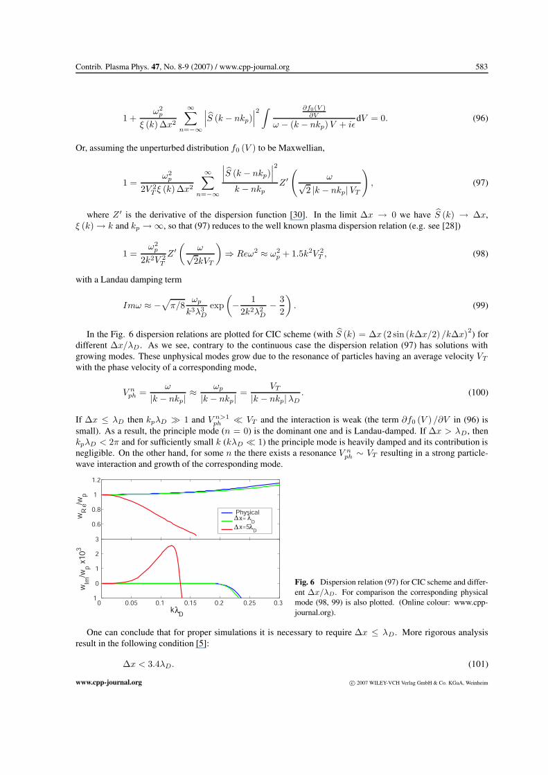
In the Fig. 6 dispersion relations are plotted for CIC scheme (with S (k) = ∆x (2 sin (k∆x/2) /k∆x)2) fordifferent ∆x/λD . As we see, contrary to the continuous case the dispersion relation (97) has solutions withgrowing modes. These unphysical modes grow due to the resonance of particles having an average velocity VT
with the phase velocity of a corresponding mode,
V nph =
ω
|k − nkp| ≈ωp
|k − nkp| =VT
|k − nkp|λD. (100)
If ∆x ≤ λD then kpλD 1 and V n>1ph VT and the interaction is weak (the term ∂f0 (V ) /∂V in (96) is
small). As a result, the principle mode (n = 0) is the dominant one and is Landau-damped. If ∆x > λD, thenkpλD < 2π and for sufficiently small k (kλD 1) the principle mode is heavily damped and its contribution isnegligible. On the other hand, for some n the there exists a resonance V n
ph ∼ VT resulting in a strong particle-wave interaction and growth of the corresponding mode.
0.6
0.8
1
1.2
wR
e/wp
0 0.05 0.1 0.15 0.2 0.25 0.3 1
0
1
2
3
wIm
/wp x
10
3
k D
Physical x=
D x=5
D
λ
∆ λ ∆ λ
Fig. 6 Dispersion relation (97) for CIC scheme and differ-ent ∆x/λD. For comparison the corresponding physicalmode (98, 99) is also plotted. (Online colour: www.cpp-journal.org).
One can conclude that for proper simulations it is necessary to require ∆x ≤ λD . More rigorous analysisresult in the following condition [5]:
∆x < 3.4λD. (101)
www.cpp-journal.org c© 2007 WILEY-VCH Verlag GmbH & Co. KGaA, Weinheim

584 D. Tskhakaya et al.: The PIC method
In the above presented analysis it has been assumed that the number of particles inside the Debye radius, ND
is large. Typically in the PIC simulations ND ≤ 103, whereas in a real plasma ND > 106. From the statisticaltheory it is known that oscillation amplitude scales as
√N (see [31]). Hence, the oscillation amplitude in PIC
simulated plasma can be much higher than in the real plasma. Moreover, this can cause unphysical oscillationswith the growth rates higher than ones predicted by theory (even if the condition (101) is satisfied). In Fig.7 the normalized growth rate of the unphysical mode is plotted as a function of ND for the CIC plasma with∆x = 10λD. As one can see the growth rate for ND ≤ 104 is significantly higher than the analytical predictionfrom (97).
Often in order to compensate effects of small number of simulated particles the corresponding densities aresmoothed. For smoothing different filtering operators are used [4]:
A′i =
WAj−1 + Ai + WAj+1
1 + 2W, W = const. (102)
Probably the most common one is so called 1-2-1 with W = 0.5. In a Fourier space for 1-2-1 filter we get
A′ (k) = sin2
(k∆x
2
)A (k) , |k|∆x ≤ π, (103)
directly indicating filtering effects for high |k| ∼ π/∆x. In order to reduce significantly the noise these filters areapplied multiple times. In Fig. 7 we plot results for the simulation when the 1-2-1 filter has been applied 5 times(per time step), indicating significant reduction of the mode growth rate.
102
103
104
105
0
0.01
0.02
0.03
0.04
ND
Imw
/wp PIC (w/o smoothing)
PIC (smoothing)
Analytic
Fig. 7 Normalized growth rate of the plasma oscillationsin 1D unmagnetized ”CIC plasma” versus ND . The case∆x = 10λD . The analytic curve is obtained from (97).
For completeness we note that in electromagnetic codes sometimes temporal filtering is also used [32].
8 Particle Collisions
8.1 Coulomb Collisions
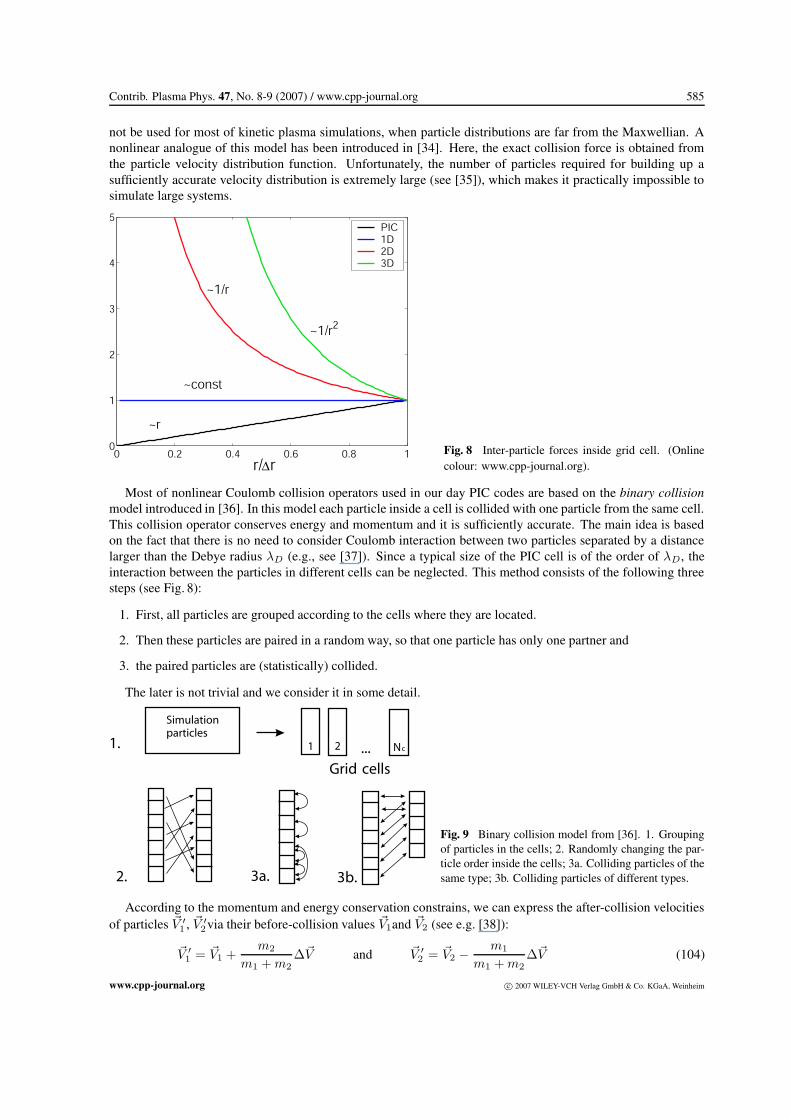
The forces acting on the particles in a classical PIC scheme correspond to macro fields, so that the simulatedplasma is assumed to be collisionless. In order to simulate a collisional plasma it is necessary to implementcorresponding routines. Moreover, the field solver is organized in such a way that self-forces are excluded,hence, the field generated by a particle inside the grid cell decreases with decreasing distance from this particle.As a result, inter-particle forces inside grid cells are underestimated (see Fig. 8). Hence, they can be (at leastpartially) compensated by introducing the Coulomb collision operator.
The first codes simulating Coulomb collisions were the particle–particle codes simulating the exact interactionbetween each particle pair. Of course this method, which scales as N 2 can not be used in modern PIC simulations.Later different MC models have been developed.
The simplest linear model assumes that the particle distribution is near to a Maxwellian and calculates anaverage force acting on particles due to collisions [33]. Although this is the fastest operator it probably can
c© 2007 WILEY-VCH Verlag GmbH & Co. KGaA, Weinheim www.cpp-journal.org
Contrib. Plasma Phys. 47, No. 8-9 (2007) / www.cpp-journal.org 585
not be used for most of kinetic plasma simulations, when particle distributions are far from the Maxwellian. Anonlinear analogue of this model has been introduced in [34]. Here, the exact collision force is obtained fromthe particle velocity distribution function. Unfortunately, the number of particles required for building up asufficiently accurate velocity distribution is extremely large (see [35]), which makes it practically impossible tosimulate large systems.
0 0.2 0.4 0.6 0.8 10
1
2
3
4
5
r/ r
PIC
1D
2D
3D
~1/r
~1/r2
~const
~r
∆Fig. 8 Inter-particle forces inside grid cell. (Onlinecolour: www.cpp-journal.org).
Most of nonlinear Coulomb collision operators used in our day PIC codes are based on the binary collisionmodel introduced in [36]. In this model each particle inside a cell is collided with one particle from the same cell.This collision operator conserves energy and momentum and it is sufficiently accurate. The main idea is basedon the fact that there is no need to consider Coulomb interaction between two particles separated by a distancelarger than the Debye radius λD (e.g., see [37]). Since a typical size of the PIC cell is of the order of λD, theinteraction between the particles in different cells can be neglected. This method consists of the following threesteps (see Fig. 8):
1. First, all particles are grouped according to the cells where they are located.
2. Then these particles are paired in a random way, so that one particle has only one partner and
3. the paired particles are (statistically) collided.
The later is not trivial and we consider it in some detail.
Simulationparticles
Grid cells
1 2 Nc...1.
2. 3a. 3b.
Fig. 9 Binary collision model from [36]. 1. Groupingof particles in the cells; 2. Randomly changing the par-ticle order inside the cells; 3a. Colliding particles of thesame type; 3b. Colliding particles of different types.
According to the momentum and energy conservation constrains, we can express the after-collision velocitiesof particles V ′
1 , V ′2via their before-collision values V1and V2 (see e.g. [38]):
V ′1 = V1 +
m2
m1 + m2∆V and V ′
2 = V2 − m1
m1 + m2∆V (104)
www.cpp-journal.org c© 2007 WILEY-VCH Verlag GmbH & Co. KGaA, Weinheim
586 D. Tskhakaya et al.: The PIC method
with ∆V = V ′ − V , V = V2 − V1, V ′ = V ′2 − V ′
1and V ′2 = V 2. As we see the calculation can be reduced tothe scattering of the relative velocity V
∆ V =(O (χ, ψ) − 1
)V , (105)
where O (χ, ψ) is the matrix corresponding to the rotation on scattering, χ, and azimuthal, ψ, angles (see [36]):
O (χ, ψ) =
⎛⎝ cos (χ) a sin (χ) sin (ψ) bx sin (χ) cos (ψ)−a sin (χ) sin (ψ) cos (χ) by sin (χ) cos (ψ)−bx sin (χ) cos (ψ) −by sin (χ) cos (ψ) cos (χ)
⎞⎠bx,y =
Vx,y
V⊥, a =
V
V⊥, V⊥ =
√V 2
x + V 2y > 0
(106)
The scattering angle χ is calculated from a corresponding statistical distribution. By using the Fokker–Plankcollision operator one can show (see [39]) that during the time ∆tc the scattering angle has the following Gaussiandistribution:
P (χ) =χ
〈χ2〉∆tc
exp
(− χ2
2 〈χ2〉∆tc
)and
⟨χ2⟩∆tc
≡ e21e
22
2πε20
n∆tcΛµ2V 3
. (107)
Here e1,2and µ = m1m2/ (m1+m2) denote the charge and reduced mass of the collided particles, respectively.n and Λ are the density and the Landau logarithm [37], respectively. The distribution (107) can be inverted to get
χ =√−2 〈χ2〉t ln R1 . (108)
Correspondingly, the azimuthal angle ψ is chosen randomly between 0 and 2π:
ψ = 2πR2 . (109)
R1and R2are random numbers between 0 and 1.Finally, the routine for two-particle collision is reduced to the calculation of expressions (104), (105), (108)
and (109). As a result each particle in a grid cell is collided just with one another particle from the same cellsaving a lot of CPU time. Interesting to note that the operator introduced in [40] collides all particles inside thecells producing just slightly more accurate relaxation times.
The Coulomb interaction is a long range interaction, when a cumulative effect of many small scattering colli-sions represents the main contribution to the collisionality. Accordingly, the time step for the Coulomb collisions∆tc should be sufficiently small:
⟨χ2⟩∆t
(V = VT ) 1. It is more convenient to formulate this condition in theequivalent following form:
νc∆tc 1 and νc =e21e
22
2πε20
nΛµ2V 3
T
, (110)
where νc is the characteristic relaxation time for the given Coulomb collisions [41] and VT is the thermal velocityof the fastest collided particle species. Although usually ∆tc ∆t, the binary collision operator is the mosttime consuming part of the PIC code. Recently, in order to speed up the collisional plasma simulations a numberof updated versions of this operator have been developed.
In [7] a new optimization method has been introduced, when all particles are intrinsically sorted according thecell where they are (see Sec. 10). Hence, the first step of the binary collision operator, i.e. grouping of particlesin the cells, can be omitted. This gives possibility to easily generalize collision operator to multiple ion speciesand effectively reduce the number of required random numbers. This saves up to 50% of the CPU time.
If plasma is nearly uniform one can introduce a cumulative binary collision operator (e.g., see [42] and [43]).In this model in spite of making a large number of light collisions, particles suffer a single large angle collision.This allows to avoid the condition (110) and significantly reduce the corresponding CPU time.
c© 2007 WILEY-VCH Verlag GmbH & Co. KGaA, Weinheim www.cpp-journal.org
Contrib. Plasma Phys. 47, No. 8-9 (2007) / www.cpp-journal.org 587
8.2 Charged-Neutral Particle Collisions
Under realistic conditions the plasma contains different neutral particles, which can collide with the plasmaparticles. The corresponding collision models used in PIC codes can be divided in two different schemes: DirectMonte-Carlo and Null collision models. The difference between these models is the way how are the collidedparticles chosen.
The direct Monte-Carlo model is a common MC scheme when all particles carry information about theircollision probability. It is a well studied technique (e.g. see [44], [45]) and frequently used in PIC simulations ofnonlinear collision processes in low temperature plasma ( [13], [14], [46]- [50]).
The classical direct MC simulation method is based on a simple expression for the collision probability
P (t) = 1 − exp(−νt), (111)
where P is the probability that particle will collide at time t, ν =∑I
i=1 νi is the sum of all possible collisionfrequencies. νi depends on local plasma parameters and energy of the given particle: νi = σi (V )ni, where V, σi
and n and are the relative velocity of collided particles, collision cross-section and the density of target particles.For simplicity we consider a linear model with cold target particles, generalization to nonlinear models can befound e.g. in [45]. According to (111) the average time between collisions can be given as
tc = − ln R
ν, (112)
with R to be a uniform random number between 0 and 1. During the simulation tc is calculated for each particleand the corresponding counter δt = 0 is activated. Particles follow a collisionless trajectories until δt = tc whena collision takes place. During the collision it is decided which kind of collision it should take place. For this arandom number R1 (between 0 and 1) is compared to the corresponding relative collision probabilities: if
R1 ≤ P1 (tc)P (tc)
=1 − exp (−ν1tc)
P (tc)≈ ν1
ν, (113)
a type 1 collision takes place; else if
R1 ≤ P1 (tc) + P2 (tc)P (tc)
≈ ν1 + ν2
ν, (114)
a type 2 collision takes place, and so on until
R1 ≤∑S
j=1 νj
ν, S ≤ I, (115)
and the collision of a type ”S” takes place. After the collision a new tc is calculated and the counter is initialized(δt = 0).
It appears that this (classical) method can not be directly applied for plasma applications: during the collision-less motion charged particles can accelerate, so that the actual collision frequency can strongly deviate from oneused for calculation of tc. An updated model has been proposed in [51], which is used in present day PIC-DirectMC codes. In this model in spite of actual collision frequency in (112) a maximum possible one is used:
tminc = − ln R
νmax. (116)
Correspondingly in (113 - 115) ν is substituted by νmax. As a results, particles are analyzed at minimum pos-sible time intervals increasing accuracy of collision operator. The difference with the expression (112) is thateffectively a ”null collision” frequency, ν0, is introduced νmax = ν + ν0 and if
R1 >ν
νmax, (117)
www.cpp-journal.org c© 2007 WILEY-VCH Verlag GmbH & Co. KGaA, Weinheim
588 D. Tskhakaya et al.: The PIC method
no collision at all takes place.
Pmax (t) = (1 − exp(−νt))max = 1 − exp (−νmax∆t). (118)
The direct MC requires that all particles have to be analyzed for a collision probability. As a result it requiressome additional memory storage and sufficiently large amount of the CPU time.
The null collision method (see [52] and [53]) requires a smaller number of particles to be sampled and it isrelatively faster. It uses the fact that in each simulation time step only a small fraction of charged particles suffercollisions with the neutrals. Hence, there is no necessity to analyze all particles. It also uses a null collisionconstrain and as a first step calculates the maximum collision probability during the PIC simulation time step ∆t:
Pmax = 1 − exp (−νmax∆t) , (119)
The maximum number of particles which can suffer a collision per ∆t time is given as Nnc = PmaxN N . Asa result only Nnc particle per time step have to be analyzed. These Nnc particles are randomly chosen, e.g., byusing the expression i = RjN with j = 1, . . . , Nnc, where i is the index of the particle to be sampled and Rj
are the random numbers between 0 and 1. The sampling procedure itself includes the calculation of the collisionprobability of a sampled particle and choosing which kind of collision it should suffer, which is similar to (113 -115): if
R ≤ P1
Pmax≈ ν1
νmax, (120)
a type 1 collision takes place; else if
R ≤ ν1 + ν2
νmax, (121)
a type 2 collision takes place, and so on. If
R >ν
νmax(122)
no collision takes place.The difference between the nonlinear and linear null collision operators is the way how the collided neutral
particles are treated. In the linear model the neutral velocity is picked up from the prescribed distribution (usuallythe Maxwellian distribution with the given density and temperature profiles). Contrary to this, in the nonlinearcase the motion of neutral particles is resolved in the simulation, and the collided ones are randomly chosen fromthe same cells, where the colliding charged-particles are located (see [15]).
When the collision partners and corresponding collision types are chosen, the collision itself takes place. Wenote that the collision models described below are equally applicable to both the direct MC and null collisionmethods. Each collision type needs a separate consideration, so that here we discuss the general principle.
The easiest collisions are the ion–neutral charge-exchange collisions. In this case the collision is reduced toan exchange of velocities:
V ′1 = V2 and V ′
2 = V1 . (123)
The recombination collisions are also easy to implement. In this case the collided particles are removed fromthe simulation and the newly born particle, i.e. the recombination product, has the velocity derived from themomentum conservation:
Vnew =m1
V1 + m2V2
mnew. (124)
The elastic collisions are treated in a similar way as the Coulomb collisions using (104). The scattering angledepends on the given atomic data. E.g., often it is assumed that the scattering is isotropic:
cosχ = 1 − 2R . (125)
c© 2007 WILEY-VCH Verlag GmbH & Co. KGaA, Weinheim www.cpp-journal.org

Contrib. Plasma Phys. 47, No. 8-9 (2007) / www.cpp-journal.org 589
In order to save computational time during the electron–neutral elastic collisions the neutrals are assumed tobe at rest. Accordingly, in spite of resolving (104) a simplified expression is used for the calculation of theafter-collision electron velocity:
V ′e ≈ Ve
√1 − 2me
Mn(1 − cosχ) . (126)
Excitation collisions are done in a similar way as the elastic ones, just before the scattering the thresholdenergy Eth is subtracted from the charged particle energy:
V ⇒ V ′ = V
√1 − Eth
E⇒ scattering ⇒ V ′′ . (127)
Important to note is that one has to take care on the proper coordinate system, e.g., in (127) the first transformshould be done in a reference system, where the collided neutral is at rest.
Implementation of inelastic collisions when secondary particles are produced is case dependent. E.g., inelectron–neutral ionization collisions, first the neutral particle is removed from the simulation and a secondaryelectron–ion pair is born. The velocity of this ion is equal to the neutral particle velocity. The velocity of electronsis calculated in the following way. First, the ionization energy is subtracted from the primary electron energy andthen the rest is divided between the primary and secondary electrons. This division is done according to givenatomic data. After finding these energies the electrons are scattered on the angles χprim and χsec. For furtherdetails see [15].
In a similar way are treated the neutral–neutral and inelastic charged–charged particle collisions.Short review of collision models including collision of particles with different weight can be found in [54].
9 Dust-plasma interactions
Recent years dusty plasma research has become a rapidly developing part of plasma physics (see [55] and refer-ences therein). Accordingly, number of PIC codes including plasma-dust interaction have been developed. Dustparticles are much heavier than the plasma ions (MDust/Mi 103), so that fully self-consistent PIC simulationincluding dust and plasma dynamics is an impossible task for our day computers. An interesting exception is thepaper [56] reporting on PIC simulations of dusty plasma with artificially reduced mass ratio MDust/Mi = 640.Typically in PIC simulations the dust particles are assumed to be immobile and the plasma-dust interaction ismodeled via electrostatic interaction of charged particles (i.e. dust represents an additional ion species) andplasma particle absorption at the dust. These codes can be divided into two parts according to the dust chargingmodel they use.
The simplified models (e.g. see [57]- [60]) use a usual PIC-MC particle collision operator for describingion (electron) absorption at the dust. The corresponding collision cross-section is obtained from analytic OrbitMotion Limited (OML) theory [61]:
σOML = πR2d
(1 − qdqi
4πε0RdEi
), (128)
where Rd, qd, qi and Ep are the dust radius and charge, and ion charge and kinetic energy, respectively. Thismodel is sufficiently fast, but can fail when plasma is strongly nonuniform and/or nonmaxwellian.
Other codes use a self-consistent model when ion trajectories are followed precisely until they are absorbed(or scattered) at the dust. In [62] - [64] the authors consider plasma interaction with a “large” size (Rd > λD)spherical dust. Dust shape and nonuniform surface charge are properly reproduced in these models ensuring highaccuracy of simulation results. One has to note, that this approach is applicable only for Rd > ∆x, so that theelectric field at the dust surface can be directly calculated from the surface charge Ed = σd/ε0. Otherwise thedust-ion interaction inside the cell and the ion motion near the dust can strongly deviate from realistic one (seeFig. (6)). In order to simulate small size dust (Rd < λD ∼ ∆x) in [65] a combined 3D PIC - molecular dynamicsimulation has been performed. The simulation domain was divided into two parts. Plasma particles inside thecell with the dust have beet treated by molecular dynamic approach, i.e. interparticle forces where calculatedaccording to the exact analytical expressions. Outside this cell a usual PIC was employed (see Fig. 10).
www.cpp-journal.org c© 2007 WILEY-VCH Verlag GmbH & Co. KGaA, Weinheim

590 D. Tskhakaya et al.: The PIC method
PIC region
MD region
Fig. 10 Computational domain for PIC-MD simulations of a dustin plasma [65]
10 Optimization of PIC codes
The PIC codes represent one of the most time consuming numerical codes used in physics. Some of heavysimulations employ up to 1010 particles, run 107 time steps and require 104 hours of CPU. Hence, optimizationof PIC code has become a necessary task. Some of optimization tools can reduce the required CPU time byfew tens of percents saving weeks of simulation time for a single processor (serial) codes. Brief reviews of PICoptimization methods can be found in [66]- [68]. Most effective ones are parallelization of the code and so calledsorting. Parallelization of numerical codes is a common technique use in all branches of numerical science. Theidea is to distribute the job between different processors. This method is case dependent, i.e. it depends on thecode to be paralleled and the machine where it will run, so that we will leave this subject out of the scope of thispaper. The interested reader can find description of this technique for PIC codes e.g. in [69], [70].
In order to understand sorting method one has to realize that the position of particle in simulation area andcomputer memory are decoupled. The neighboring (in computer memory) particles can be far away from eachother in the simulation area suffering different forces and different physics (see. Fig. 8a). Hence, runningover particle index the routines like particle weighting, particle mover and collision operators have to operatewith different external variables (fields, densities) at different grid points. As a result, the probability that thisvalues will be found in a fast (cache) memory can be low. In order to increase the probability of cache hitnumber of authors [66], [71]- [73] introduce particle sorting according to the grid cells. The sorting routine areapplied before calling the particle mover and weighting operations, so that operations on neighboring particlesrequire the same external variables (see Fig. 11b). As it was demonstrated in [73] by introducing a fast sortingoperator the simulation speed can increase up to 70%. In [74] and [7] the authors went further developing a newmethods of particle representation in memory based on their position. In [74] particle array has a strict structure,which is ordered according to spatial cells: e.g. particles from first cell are first particles in the array, followedby the particles from the second cell and so on. In order to distinguish different cells an additional array isintroduced where indexes of the last particles of each cell are saved. In [7] particle array has an additional indexcorresponding to the cell index. E.g. for a 1D code the particle coordinate is represented as the array x[i][j][k],where i, j and k indexes correspond to the particle type, cell index and particle index inside the given cell. Itappears that the memory representation of this type can be successfully used also in collision operators reducingcorresponding CPU time up to 50%.
Although PIC codes represent attractive tools for plasma simulations, they have number of disadvantages,which restrict applicability of these codes. This drives an interest for developing of new tools, which are able tosubstitute PIC codes in some applications. One of this approaches is the grid-free model based on the treecodealgorithm. Originally the treecode method was developed for astrophysical applications [75], but later it wassuccessfully used for plasma simulations too (see [76]- [80]). The idea of the treecode method is to divideparticle-particle interaction into two groups:
c© 2007 WILEY-VCH Verlag GmbH & Co. KGaA, Weinheim www.cpp-journal.org
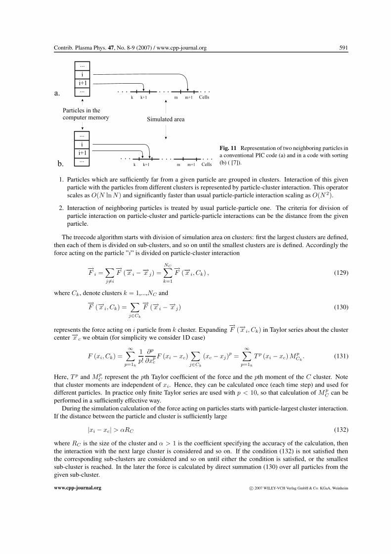
Contrib. Plasma Phys. 47, No. 8-9 (2007) / www.cpp-journal.org 591
...
...
i
Particles in thecomputer memory
i+1
...
...
i
i+1
Simulated area
k k+1 m m+1 Cells
k k+1 m m+1 Cells
a.
b.
Fig. 11 Representation of two neighboring particles ina conventional PIC code (a) and in a code with sorting(b) ( [7]).
1. Particles which are sufficiently far from a given particle are grouped in clusters. Interaction of this givenparticle with the particles from different clusters is represented by particle-cluster interaction. This operatorscales as O(N ln N) and significantly faster than usual particle-particle interaction scaling as O(N 2).
2. Interaction of neighboring particles is treated by usual particle-particle one. The criteria for division ofparticle interaction on particle-cluster and particle-particle interactions can be the distance from the givenparticle.
The treecode algorithm starts with division of simulation area on clusters: first the largest clusters are defined,then each of them is divided on sub-clusters, and so on until the smallest clusters are is defined. Accordingly theforce acting on the particle ”i” is divided on particle-cluster interaction
−→F i =
∑j =i
−→F (−→x i −−→x j) =
NC∑k=1
−→F (−→x i, Ck) , (129)
where Ck, denote clusters k = 1,...,NC and−→F (−→x i, Ck) =
∑j∈Ck
−→F (−→x i −−→x j) (130)
represents the force acting on i particle from k cluster. Expanding−→F (−→x i, Ck) in Taylor series about the cluster
center −→x c we obtain (for simplicity we consider 1D case)
F (xi, Ck) =∞∑
p=1k
1p!
∂p
∂xpcF (xi − xc)
∑j∈Ck
(xc − xj)p =
∞∑p=1k
T p (xi − xc)MpCk
. (131)
Here, T p and MpC represent the pth Taylor coefficient of the force and the pth moment of the C cluster. Note
that cluster moments are independent of xi. Hence, they can be calculated once (each time step) and used fordifferent particles. In practice only finite Taylor series are used with p < 10, so that calculation of M p
C can beperformed in a sufficiently effective way.
During the simulation calculation of the force acting on particles starts with particle-largest cluster interaction.If the distance between the particle and cluster is sufficiently large
|xi − xc| > αRC (132)
where RC is the size of the cluster and α > 1 is the coefficient specifying the accuracy of the calculation, thenthe interaction with the next large cluster is considered and so on. If the condition (132) is not satisfied thenthe corresponding sub-clusters are considered and so on until either the condition is satisfied, or the smallestsub-cluster is reached. In the later the force is calculated by direct summation (130) over all particles from thegiven sub-cluster.
www.cpp-journal.org c© 2007 WILEY-VCH Verlag GmbH & Co. KGaA, Weinheim
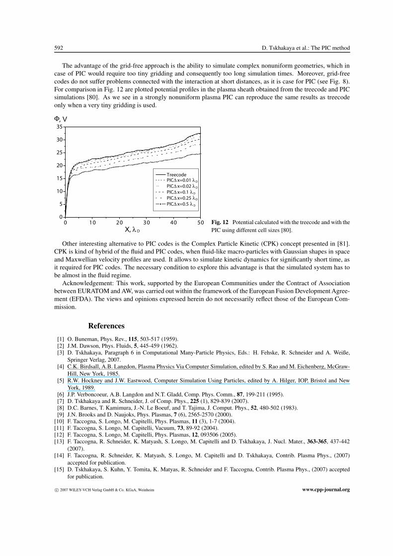
592 D. Tskhakaya et al.: The PIC method
The advantage of the grid-free approach is the ability to simulate complex nonuniform geometries, which incase of PIC would require too tiny gridding and consequently too long simulation times. Moreover, grid-freecodes do not suffer problems connected with the interaction at short distances, as it is case for PIC (see Fig. 8).For comparison in Fig. 12 are plotted potential profiles in the plasma sheath obtained from the treecode and PICsimulations [80]. As we see in a strongly nonuniform plasma PIC can reproduce the same results as treecodeonly when a very tiny gridding is used.
0 10 20 30 4 00
5
10
15
20
25
30
35
TreecodePIC∆ x=0.01 λ D
PIC∆ x=0.02 λ D
PIC∆ x=0.1 λ D
PIC∆ x=0.25 λD
PIC∆ x=0.5 λ D
, V
X, λ D
Φ
0 5 Fig. 12 Potential calculated with the treecode and with thePIC using different cell sizes [80].
Other interesting alternative to PIC codes is the Complex Particle Kinetic (CPK) concept presented in [81].CPK is kind of hybrid of the fluid and PIC codes, when fluid-like macro-particles with Gaussian shapes in spaceand Maxwellian velocity profiles are used. It allows to simulate kinetic dynamics for significantly short time, asit required for PIC codes. The necessary condition to explore this advantage is that the simulated system has tobe almost in the fluid regime.
Acknowledgement: This work, supported by the European Communities under the Contract of Associationbetween EURATOM and AW, was carried out within the framework of the European Fusion Development Agree-ment (EFDA). The views and opinions expressed herein do not necessarily reflect those of the European Com-mission.
References[1] O. Buneman, Phys. Rev., 115, 503-517 (1959).[2] J.M. Dawson, Phys. Fluids, 5, 445-459 (1962).[3] D. Tskhakaya, Paragraph 6 in Computational Many-Particle Physics, Eds.: H. Fehske, R. Schneider and A. Weiße,
Springer Verlag, 2007.[4] C.K. Birdsall, A.B. Langdon, Plasma Physics Via Computer Simulation, edited by S. Rao and M. Eichenberg, McGraw-
Hill, New York, 1985.[5] R.W. Hockney and J.W. Eastwood, Computer Simulation Using Particles, edited by A. Hilger, IOP, Bristol and New
York, 1989.[6] J.P. Verboncoeur, A.B. Langdon and N.T. Gladd, Comp. Phys. Comm., 87, 199-211 (1995).[7] D. Tskhakaya and R. Schneider, J. of Comp. Phys., 225 (1), 829-839 (2007).[8] D.C. Barnes, T. Kamimura, J.-N. Le Boeuf, and T. Tajima, J. Comput. Phys., 52, 480-502 (1983).[9] J.N. Brooks and D. Naujoks, Phys. Plasmas, 7 (6), 2565-2570 (2000).
[10] F. Taccogna, S. Longo, M. Capitelli, Phys. Plasmas, 11 (3), 1-7 (2004).[11] F. Taccogna, S. Longo, M. Capitelli, Vacuum, 73, 89-92 (2004).[12] F. Taccogna, S. Longo, M. Capitelli, Phys. Plasmas, 12, 093506 (2005).[13] F. Taccogna, R. Schneider, K. Matyash, S. Longo, M. Capitelli and D. Tskhakaya, J. Nucl. Mater., 363-365, 437-442
(2007).[14] F. Taccogna, R. Schneider, K. Matyash, S. Longo, M. Capitelli and D. Tskhakaya, Contrib. Plasma Phys., (2007)
accepted for publication.[15] D. Tskhakaya, S. Kuhn, Y. Tomita, K. Matyas, R. Schneider and F. Taccogna, Contrib. Plasma Phys., (2007) accepted
for publication.
c© 2007 WILEY-VCH Verlag GmbH & Co. KGaA, Weinheim www.cpp-journal.org
Contrib. Plasma Phys. 47, No. 8-9 (2007) / www.cpp-journal.org 593
[16] J.P. Verboncoeur, M.V. Alves, V. Vahedi, and C.K. Birdsall, J. Comput. Phys., 104 (2), 321-328 (1993).[17] D. Tskhakaya and S. Kuhn, Contrib. Plasma Phys., 42 (2-4), 302-308 (2002).[18] K.L. Cartwright, J.P. Verboncoeur and C.K. Birdsall, J. Comput. Phys., 162 (2), 483-513 (2000).[19] H.C. Kim, Y. Feng and J.P. Verboncoeur, J. Comput. Phys., 223 (2), 629-642 (2007).[20] D. Tskhakaya and S. Kuhn, Plasma Phys. Control. Fusion, 47, A327-A337 (2005).[21] J.P. Verboncoeur, J. Comput. Phys., 174, 421-427 (2001).[22] W.M. Ruyten, J. Comput. Phys., 105, 224-234 (1993).[23] D.J. Larson, D.W. Hewett, and A.B. Langdon, Comput. Phys. Comm., 90 (2-3), 260-266 (1995).[24] F. Collino, T. Fouquet, P. Joly, J. Comput. Phys., 211, 9-35 (2006).[25] P.N. Swarztrauber, SIAM J. Numer. Anal., 11 (6), 1136-1150 (1974).
See also http://www.cisl.ucar.edu/css/software/fishpack/.[26] V. Vahedi, G. DiPeso, J. Comp. Phys., 131, 149 (1997).[27] W.H. Press, S.A. Teukolsky, W.T. Vetterling, B.P. Flannery, Numerical Recipes in C, Cambridge University Press,
Cambridge, New York Port Chester, Melbourne, Sydney, 2002.[28] N.A. Krall and A.W. Trivelpiece, Principles of Plasma Physics, San Francisco Press, 1986.[29] L.D. Landau, J. Phys. (USSR), 10, 25-34 (1946).[30] B.D. Fried and S.D. Conte, The Plasma Dispersion Function, Academic Press, New York 1961.[31] L.D. Landau, E.M. Lifshits, Statistical physics, .Elsevier Science & Technology (UK), 1996.[32] P.W. Rambo, J. Ambrosiano, A. Friednam, and D.E. Nielsen Jr., Proceedings of 13th Conference on the Numerical
Simulation of Plasmas, Santa Fe, New Mexico 1989.[33] A. Bergmann, Contrib. Plasma Phys., 38, 231 (1998).[34] O.V. Batishchev, X.Q. Xu, J.A. Byers, R.H. Cohen, S.I. Krasheninnikov, T.D. Rognlien, and D.J. Sigmar, Phys. Plasmas,
3 (9), 3386-3396 (1996).[35] O.V. Batishchev, S.I. Krasheninnikov, P.J. Catto, et al, Phys. Plasmas, 4 (5), 1672-1680 (1997).[36] T. Takizuka and H. Abe, J. Comput. Phys., 25 (3), 205-219 (1977).[37] N.A. Krall and A.W. Trivelpiece, Principles of Plasma Physics, San Francisco Press, Inc., Box 6800, San Francisco,
1986.[38] L.D. Landau and E.M. Lifshitz, Course of Theoretical Physics, Vol. 1, Mechanics, Pergamon Press, Oxford-London-
Paris, 1960.[39] R. Shanny, J.M. Dawson, and J.M. Greene, Phys. Fluids, 10 (6), 1281-1287 (1967).[40] W.X. Wang, M. Okamoto, N. Nakajima, and S. Murakami, J. Comput. Phys., 128 (1), 209-222 (1996).[41] D.L. Book, NRL Plasma formulary, Naval Research Laboratory, Washington D.C., 1978.[42] K. Nanbu, Phys. Rev., E 55 (4), 4642-4652 (1997).[43] A.V. Bobylev and K. Nanbu, Phys. Rev., E 61 (4), 4576-4586 (2000).[44] G.A. Bird, Molecular Gas Dynamics and the Direct Simulation of Gas Flows, Oxford: Oxford Science, 1994.[45] S. Longo, Plasma Sources Sci. Technol. 15, 181-188 (2006).[46] V.V. Serikov, S. Kawamoto, K. Nambu, IEEE Trans. Plasma Sc., 27 (5), 1389-1398 (1999).[47] K. Matyash, R. Schneider, A. Bergmann, W. Jacobb, U. Fantz, P. Pecher, J. Nucl. Mater., 313-316, 434-438 (2003).[48] F. Taccogna, R. Schneider, S. Longo, M. Capitelli, Phys. Plasmas, 14, 073503 (2007).[49] F. Taccogna, R. Schneider, S. Longo, and M. Capitelli, Rev. Sci. Instrum., (2007) accepted for publication.[50] F. Taccogna, S. Longo, M. Capitelli, and R. Schneider, IEEE Trans Plasma Sci., (2007) accepted for publication.[51] H.R. Skullerud, J. Phys. D: Appl. Phys., 1, 1567-1569 (1968).[52] C.K. Birdsall, IEEE Trans. Plasma Sc., 19 (2), 65-85 (1991).[53] V. Vahedi, M. Surendra, Comp. Phys. Comm., 87, 179-198 (1995).[54] K. Nambu, IEEE Trans. Plasma Sc., 28 (3), 971-990 (2000).[55] P.K. Shukla and A.A. Mamun, Introduction to Dusty Plasma Physics, IoPP, Bristol and Phyladelphia, 2002.[56] K. Matyash, R. Schneider, Contrib. Plasma Phys., 44 (1-3), 157-161 (2004).[57] O. Yu. Kravchenko, Yu.I. Chutov, W.J. Goedheer, R.D. Smirnov and S. Takamura, J. Nucl. Mater., 313-316, 1109-1113
(2003).[58] Yu.I. Chutov, O.Yu. Kravchenko, S. Masuzaki, A. Sagara, R.D. Smirnov, Yu. Tomita, Contrib. Plasma Phys., 44 (1-3),
138-143 (2004).[59] R. Smirnov, Y. Tomita, T. Takizuka, A. Takayama, Yu. Chutov, Contrib. Plasma Phys., 44 (1-3), 150-156 (2004).[60] W.J. Goedheer, M.R. Akdim, Yu.I. Chutov, Contrib. Plasma Phys., 44 (1-3), 395-404 (2004).[61] J.E. Allen, Phys. Scripta, 45, 497-503 (1992).[62] I.H. Hutchinson, Plasma Phys. Control. Fusion, 45(8), 1477-1500 (2003).[63] I.H. Hutchinson, Plasma Phys. Control. Fusion, 47(1), 71-87 (2005).[64] R. Smirnov, Y. Tomita, D. Tskhakaya, and T. Takizuka, Contrib. Plasma Phys., 46 (7-9), 623-627 (2006).[65] K. Matyash, R. Schneider, F. Taccogna and D. Tskhakaya, J. Nucl. Mater., 363-365, 458-461 (2007).[66] V.K. Decyk, S.R. Karmesin, A. de Boer, P.C. Liewer, Comput. Phys., 10, 290-298 (1996).[67] E. Kawamura, C.K. Birdsall and V. Vahedi, Plasma Sources Sci. Technol., 9 (3), 413-428 (2000).
www.cpp-journal.org c© 2007 WILEY-VCH Verlag GmbH & Co. KGaA, Weinheim
594 D. Tskhakaya et al.: The PIC method
[68] J.D. Blahovec, Jr., L.A. Bowers, J.W. Luginsland, Member, IEEE, G.E. S. Sasser, and J.J.Watrous, IEEE Trans. PlasmaSc., 28 (3), 821-829 (2000).
[69] V.K. Decyk, Comp. Phys. Comm., 87, 87-94 (1995).[70] V.K. Decyk, Ch.D. Norton, Comp. Phys. Comm., 164, 80-85 (2004).[71] D.V. Anderson, D.E. Shumaker, Comp. Phys. Comm., 87 16-34 (1995).[72] T. MacFarland, H.M.P. Couchman, R.F. Pearce, J. Pichlmeier, New Astron., 3, 678-705 (1998).[73] K.J. Bowers, J. Comput. Phys., 173, 393-411 (2001).[74] R.J. Thacker, H.M.P. Couchman, Comp. Phys. Comm., 174, 540-554 (2006).[75] J. Barnes and P. Hut, Nature, 324, 446-449 (1986).[76] S. Pfalzner and P. Gibbon, Many-Body Tree Methods in Physics, Cambridge, U.K.: Cambridge Univ. Press, 1996.[77] S. Pfalzner and P. Gibbon, Phys. Rev. E, 57, 4698-4705 (1998).[78] A.J. Christlieb, R. Krasny, and J.P. Verboncoeur, IEEE Trans Plasma Sci, 32, 384-389 (2004).[79] A.J. Christlieb, R. Krasny and J.P. Verboncoeur, Comput. Phys. Comm., 164, 306-310 (2004).[80] K. Matyash , R. Schneider, R. Sydora and F. Taccogna, Contrib. Plasma Phys., to be published (2007).[81] D.W. Hewett, J. Comput. Phys., 189, 390-426 (2003).
c© 2007 WILEY-VCH Verlag GmbH & Co. KGaA, Weinheim www.cpp-journal.org
Copyright © 2022 FDOKUMEN