A parallel, implicit, cell‐centered method for two‐phase flow with a preconditioned NewtonKrylov...

Computational Geosciences 1 (1997) 215–249 215

A parallel, implicit, cell-centered method for two-phaseflow with a preconditioned Newton–Krylov solver ∗

Clint N. Dawson a, Hector Klıe b,∗∗, Mary F. Wheeler a and Carol S. Woodward c,∗∗∗

a Texas Institute for Computational and Applied Mathematics, University of Texas, Austin, TX 78712,USA

E-mail: clint;[email protected] Department of Computational and Applied Mathematics, Rice University, Houston, TX 77251, USA

E-mail: [email protected] Center for Applied Scientific Computing, Lawrence Livermore National Laboratory, Livermore,

CA 94551, USAE-mail: [email protected]

Received 29 August 1996; revised 27 June 1997

A new parallel solution technique is developed for the fully implicit three-dimensionaltwo-phase flow model. An expanded cell-centered finite difference scheme which allowsfor a full permeability tensor is employed for the spatial discretization, and backward Euleris used for the time discretization. The discrete systems are solved using a novel inexactNewton method that reuses the Krylov information generated by the GMRES linear iterativesolver. Fast nonlinear convergence can be achieved by composing inexact Newton steps withquasi-Newton steps restricted to the underlying Krylov subspace. Furthermore, robustnessand efficiency are achieved with a line-search backtracking globalization strategy for thenonlinear systems and a preconditioner for each coupled linear system to be solved. Thisinexact Newton method also makes use of forcing terms suggested by Eisenstat and Walkerwhich prevent oversolving of the Jacobian systems. The preconditioner is a new two-stagemethod which involves a decoupling strategy plus the separate solutions of both nonwetting-phase pressure and saturation equations. Numerical results show that these nonlinear andlinear solvers are very effective.

1. Introduction

Multiphase flow in permeable media arises in a number of important applications,including reservoir and aquifer characterization, simulation of enhanced oil recoveryprocesses, and the study of soil and groundwater contamination. Multiphase flow ismodeled by coupled systems of partial differential and algebraic equations. Solvingthese equations numerically is complicated by many factors, including nonlinearities

∗ This work was supported by the United States Department of Energy and Intevep.∗∗ Support of this author has been provided by Intevep S.A., Los Teques, Edo. Miranda, Venezuela.∗∗∗ This author was supported, in part, under the auspices of the U.S. Department of Energy by Lawrence

Livermore National Laboratory under contract number W-7405-Eng-48.

Baltzer Science Publishers BV

216 C.N. Dawson et al. / Two-phase flow model

in the model, sharp fluid fronts, wells, mass transfer, heterogeneities in rock andfluid properties, gravity and capillary pressure effects. Robust implementations ofmultiphase flow models have proven to be computationally intensive. Moreover, withthe advent of distributed memory parallel computers, new solution strategies must bedeveloped which can effectively utilize these architectures.

In this paper we describe the development and implementation of a parallel sim-ulator for two-phase flow. We employ the expanded mixed finite element method ofArbogast et al. [2] for spatial discretization combined with backward differencing intime. This discretization results in a nonlinear system of equations which must besolved at every time step. For solving this system we use a global inexact Newtonmethod [18]. The Newton equation is solved with a preconditioned version of GMRES.While the use of Newton’s method combined with GMRES is a fairly standard solutionstrategy, we will present some novel ideas and extensions on how to implement thismethod more robustly, efficiently and in parallel. We remark that the two-phase flowmodel has been chosen merely as a prototype for more complex multiphase composi-tional models. The numerical methods we study here are generalizable to these morecomplicated models.

Because of its mass-conservation and approximation properties, the mixed finiteelement method disguised as a cell-centered finite difference scheme has long been usedto simulate multiphase flow [33]. The advantage of the expanded mixed method overthe standard mixed method is that, with certain approximating spaces and quadraturerules, it allows for a full permeability tensor and still reduces to an accurate cell-centered finite difference scheme. A full tensor can arise as the result of computing“effective” permeabilities from upscaling [17], or from mapping a rectangular gridinto a logically rectangular grid with curvilinear elements [1]. This generality addsflexibility to the types of problems which can be modeled. The accuracy of theexpanded method was examined in [1,2] for single phase flow. There it was shownthat the pressures and velocities are super-convergent at cell centers and cell edges,respectively, similar to the standard mixed method.

The global inexact Newton method we have used to solve the nonlinear sys-tems arising at each time step consists of two complementary parts, the line-searchbacktracking method and the selection of forcing terms [19]. The first part imposesa sufficient decrease condition on the norm of the nonlinear function, and the latterdictates the local convergence of the linear system. The correct selection of forcingterms plays an important role in avoiding oversolution of the Newton equation, andits application to problems in subsurface simulation is novel.

The GMRES algorithm is enhanced by a two-stage preconditioner suggested byKlıe et al. [29]. The preconditioner is comprised of two inner iterations which solvefor both pressures and saturations to an acceptable level of accuracy. A cheap buteffective decoupling strategy allows the relatively easy solution of these two types ofvariables compared to the original system which is indefinite and highly nonsymmetric.Therefore, the decoupling strategy itself acts as a preliminary preconditioning stage.This scheme represents a more effective and robust version of the IMPES (see [21])

C.N. Dawson et al. / Two-phase flow model 217

type of preconditioner suggested by Wallis [36] which relies upon the pressure solutionof one phase. In fact, it was observed that in the event of high changes of saturations(numerically induced by larger time steps) Wallis’ preconditioner shows limitationsthat were even more severe for the full permeability tensor cases pursued in this work.

The solver presented in this work uses information generated as part of theGMRES process. The Krylov basis built within the Arnoldi process is used as asearch engine for generation of new Newton directions without explicit manipulationof the Jacobian (approximation) at the new point. This can be efficiently carried out byapplying Broyden updates (see [16]) to the upper Hessenberg matrix (of much lowerorder than the original Jacobian) resulting from the Arnoldi factorization. Subsequentupdates can be performed until the underlying Krylov basis is unable to generate adecrease direction for the nonlinear function norm. This method is fully described in[28] and serves as a vehicle for achieving faster convergence rates than those givenby standard inexact Newton implementations.

The paper is outlined as follows. In section 2, we present the equations governingtwo-phase flow in porous media. In section 3, we describe the fully implicit discretiza-tion of the two-phase mathematical model. Section 4 is devoted to the description ofthe main components of the global inexact Newton method, line-search backtrackingand the selection of forcing terms. In section 5, we discuss the philosophy of thehigher-order Newton–Krylov iterative solver for nonlinear equations. We also includea discussion of the two-stage preconditioner. In section 6, we present issues consideredfor efficient implementation of the ideas described in previous sections. Our approachis validated and illustrated through numerical examples in section 7. We end this workwith some concluding remarks and directions of future research in section 8.

2. Model formulation

We consider the simultaneous flow of two immiscible phases through a porousmedium. For example, one phase may consist of oil (nonwetting phase) and the otherof water (wetting phase). Two phase flow models can also be used to simulate theinfiltration of water (possibly contaminated) through unsaturated media and into thewater table [7,23]. In this case, the wetting phase is also water but the nonwettingphase is air.

Conservation of mass for each of the two phases leads to the pair of equations,

∂(φρwsw)∂t

+∇ · (ρwuw) = qw, (1)

∂(φρnsn)∂t

+∇ · (ρnun) = qn, (2)

where sl is the saturation of phase l, ρl is the density of phase l, φ is the porosity of


the medium, t is time, ql is a source/sink term for phase l and ul is the Darcy velocityfor phase l expressed as

ul = −krlKµl

(∇pl − ρlg∇D), l = n, w. (3)

Here K is the absolute permeability tensor, krl is the relative permeability of phase l,µl is the viscosity of phase l, pl is the pressure of phase l, g is the gravitationalacceleration constant and D is depth. The subscript l refers to the wetting (w) ornonwetting (n) phase. We let λl = krlK/µl denote the mobility of phase l.

The pressures and saturations of the two phases are related by the capillarypressure and the assumption that the two phases fill the pore space,

pc(sw) = pn − pw, (4)

1 = sn + sw. (5)

Boundary conditions of the form,

σuw · n + νpw = γw, (6)

σun · n + νpn = γn, (7)

are allowed where σ and ν are spatially varying coefficients, n is the outward, unit,normal vector to the boundary of the domain and γl is a spatially varying function.

We specify pn and sw initially and use a hydrostatic equilibrium condition tosolve for an initial value of sn.

Each phase is assumed to be slightly compressible with the densities given interms of pressure by the equation of state,

ρl(pl) = ρlbeclpl , (8)

where cl is the compressibility constant for phase l and ρlb is the density of phase l atsome reference depth.

The system of coupled nonlinear equations (1)–(8) makes up the mathematicalmodel for the two-phase flow problem. Substituting (3)–(8) into (1)–(2), one obtainsa system of two equations in two unknowns. Frequently, the primary unknowns arepressures and saturations of one phase or of two different phases. All other quantitiesdepend upon these unknowns and/or on the independent variables, time and position.

Equations (1) and (2) can be manipulated into a parabolic “pressure” equation anda nonlinear convection–diffusion equation for saturation. The pressure equation be-comes an elliptic equation for incompressible fluids. This reformulation of the problemis used when applying implicit pressure–explicit saturation (IMPES) [4] or sequentialtime-stepping [14] approaches. These time-stepping techniques effectively decouplethe equations, allowing for appropriate numerical techniques to be applied to each pieceof the equation, at the expense of a time-step constraint to maintain stability of thenumerical solutions [31]. In this paper, we will examine fully implicit time-stepping,where (1)–(2) are solved simultaneously using a nonlinear iterative method. In theory,


this approach does not have any stability time-step constraints. Moreover, when simu-lating more complex physical problems, such as multiphase compositional or thermalprocesses, one needs to more closely couple the equations in the solution process.Thus, we view the fully implicit two phase model discussed here as a prototype formore complex porous media flow models.

3. Discretization scheme

We now describe the finite difference scheme employed in solving the system(1)–(7).

We consider a rectangular two or three dimensional domain, Ω, with boundary∂Ω. We let L2(Ω) denote the Banach space consisting of square integrable functionsover Ω, i.e.,

L2(Ω) =

f :∫

Ωf 2 <∞

,

and we let (·, ·) denote the L2(Ω) inner product, scalar and vector, where for f and gin L2(Ω),

(f , g) =

∫Ωfg dΩ.

We will approximate the L2 inner product with various quadrature rules, denotingthese approximations by (·, ·)R, where R = M, T and TM are application of themidpoint, trapezoidal and trapezoidal by midpoint rules, respectively.

Let 0 = t0 < t1 < · · · < tN = T be a given sequence of time steps, ∆tn =tn − tn−1, ∆t = maxn ∆tn, and for φ = φ(·, t), let φn = φ(·, tn) with

dtφn =

φn − φn−1

∆tn.

Let

V = H(Ω, div) =

v ∈(L2(Ω)

)d: ∇ · v ∈ L2(Ω)

and W = L2(Ω).

We will consider a quasi-uniform partitioning of Ω with mesh size h denotedby T and consisting of parallelepipeds. Thus T is obtained through the cross-productof partitions in each coordinate direction. Let xi+1/2, i = 0, . . . ,Nx, denote theendpoints of the intervals for the partition along the x coordinate axis, with similardefinitions for yj+1/2, j = 0, . . . ,Ny, and zk+1/2, k = 0, . . . ,Nz. The totalnumber of blocks nb = NxNyNz . Therefore, the vertices of element Eijk ∈ Tare the (xi±1/2, yj±1/2, zk±1/2). We denote the midpoint of Eijk by (xi, yj , zk). Let∆xi = xi+1/2 − xi−1/2 with similar definitions for ∆yj and ∆zk. Moreover, denote by∆xi+1/2 the average of ∆xi and ∆xi+1.


We consider the lowest order Raviart–Thomas–Nedelec space on bricks [32,34].Thus, on any element E ∈ T , we have

Vh(E) =

(α1x+ β1,α2y + β2,α3z + β3): αi,βi ∈ R

,

Wh(E) = α: α ∈ R.

For an element on the boundary, ∂E ⊂ ∂Ω, we have the edge space,

Λh(∂E) = α: α ∈ R.

We use the standard nodal basis. For Vh the nodes are at the midpoints of edgesor faces of the elements; for example, for a function U ∈ Vh the x-component of U,Ux, is defined by its values at the points (xi+1/2, yj , zk). For Wh the nodes are at themidpoints of the elements, and for Λh the nodes are at midpoints of edges.

For a given phase, the expanded mixed finite element method simultaneouslyapproximates sl, pl, (uxl , uyl , uzl ) ≡ ul = −∇pl + ρlg∇D and (uxl ,uyl ,uzl ) ≡ ul =ρlλlul. This method with quadrature, applied to either phase, is given as follows.Find Snl ∈ Wh, Pnl ∈ Wh, Un

l ∈ Vh, Unl ∈ Vh and αnl ∈ Λh for each n = 1, . . . ,N

satisfying(dt(φρlS

nl

),w)

M =−(∇ ·Un

l ,w)

+(qnl ,w

)M

, ∀w ∈Wh, (9)(Unl , v)

TM =(Pnl ,∇ · v

)−(αnl , v · n

)Γ +

(ρnl g∇D, v

)TM, ∀v ∈ Vh, (10)(

Unl , v)

TM =(ρlλ

nl Un

l , v)

T, ∀v ∈ Vh, (11)(σUn

l · n,β)

Γ =(γl − ναnl ,β

)Γ, ∀β ∈ Λh. (12)

Note that αnl approximates pnl on Γ.The system (9)–(12) coupled with the algebraic equations (4)–(5) reduces to a

finite difference scheme for the pressure and saturation approximations. To see this,consider first equation (9) and let w = wijk ∈Wh be the basis function,

wijk =

1, in Eijk,0, otherwise.

Then, dropping the phase subscript, we find

∆xi∆yj∆zkφijk((ρS)nijk − (ρS)n−1

ijk

)= ∆tn∆yj∆zk

( (Ux)ni+1/2,j,k − (Ux)ni−1/2,j,k

∆xi+1/2

)+ ∆tn∆xi∆zk

( (Uy)ni,j+1/2,k − (Uy)ni,j−1/2,k

∆yj+1/2

)+ ∆tn∆xi∆yj

( (Uz)ni,j,k+1/2 − (Uz)ni,j,k−1/2

∆zk+1/2

)+ ∆tn∆xi∆yj∆zkqnijk. (13)


Equation (10) gives Un in terms of Pn; in particular, choosing v =(vi+1/2,j,k(x), 0, 0), where vi+1/2,j,k is the basis function associated with node(xi+1/2, yj , zk),

vi+1/2,j,k =

1∆xi

(x− xi−1/2), x ∈ [xi−1/2,xi+1/2], y ∈ [yj−1/2, yj+1/2],

z ∈ [zk−1/2, zk+1/2],1

∆xi+1(xi+3/2 − x), x ∈ [xi+1/2,xi+3/2], y ∈ [yj−1/2, yj+1/2],

z ∈ [zk−1/2, zk+1/2],0, otherwise,

(10) reduces to (dropping temporal superscripts)

Uxi+1/2,j,k =Pijk − Pi+1,j,k

∆xi+1/2+ ρi+1/2,j,kg

Di+1,j,k −Dijk

∆xi+1/2, (14)

where ρi+1/2,j,k = (ρi+1,j,k + ρijk)/2, and we have approximated the x componentof ∇D at (xi+1/2, yj , zk) by central differences. If xi+1/2 is on the boundary, thenthe difference in pressures in equation (14) is replaced by the difference between thepressure in the nearest cell and the multiplier α on the boundary closest to the cell.The divisor for this difference will be half the cell width instead of ∆xi+1/2. Theα term only plays a role on the outer boundary of the domain.

Equation (11) gives U in terms of U. Letting v be chosen as in (11) gives

Uxi+1/2,j,k∆xi+1/2

=18

(ρkrµ

)i+1/2,j,k

[(K11,i+1/2,j−1/2,k−1/2 +K11,i+1/2,j+1/2,k−1/2

+K11,i+1/2,j−1/2,k+1/2 +K11,i+1/2,j+1/2,k+1/2)

×(∆xiUxi+1/2,j,k + ∆xi+1U

xi+1/2,j,k

)+ (K12,i+1/2,j−1/2,k−1/2 +K12,i+1/2,j−1/2,k+1/2)

×(∆xiUyi,j−1/2,k + ∆xi+1U

yi+1,j−1/2,k

)+ (K12,i+1/2,j+1/2,k−1/2 +K12,i+1/2,j+1/2,k+1/2)

×(∆xiUyi,j+1/2,k + ∆xi+1U

yi+1,j+1/2,k

)+ (K13,i+1/2,j−1/2,k−1/2 +K13,i+1/2,j+1/2,k−1/2)

×(∆xiUzi,j,k−1/2 + ∆xi+1U

zi+1,j,k−1/2

)+ (K13,i+1/2,j−1/2,k+1/2 +K13,i+1/2,j+1/2,k+1/2)

×(∆xiUzi,j,k+1/2 + ∆xi+1U

zi+1,j,k+1/2

)]≡(ρkrµ

)i+1/2,j,k

Uxi+1/2,j,k. (15)


The coefficient (ρkr/µ)i+1/2,j,k is approximated by upstream weighting as deter-mined by the sign of Uxi+1/2,j,k, i.e.,

(ρkrµ

)i+1/2,j,k

=

(ρkrµ

)i+1,j,k

, if Uxi+1/2,j,k < 0,(ρkrµ

)ijk

, otherwise.

Lastly, equation (12) defines the multipliers α on the domain boundary. Forexample, in (12) letting β = β1/2,j,k, where β1/2,j,k = 1 on the edge with midpoint(x1/2, yj , zk) and zero elsewhere, we have

−σUx1/2,j,k = γ1/2,j,k − να1/2,j,k. (16)

Combining equations (13)–(16) and applying similar ideas to the y and z direc-tions gives a finite difference method for pressure and saturation approximations, witha 19-point stencil (see figure 1). Writing finite difference schemes for both phasesgives our coupled system of nonlinear discrete equations.

3.1. Algebraic system of equations

Taking nonwetting phase pressures and saturations as primary unknowns andapplying Newton’s method to linearize the above finite difference scheme, we obtaina linear algebraic system of equations whose associated matrix is the Jacobian. Eachrow of the Jacobian expresses the dependence of either a wetting or nonwetting phaselinearized conservation equation at a grid cell on the nonwetting phase pressures andsaturations. The nonwetting phase linearized equations depend on 19 pressures andon 7 saturations. The wetting phase linearized equations depend on 19 pressures and,due to capillary pressure effects, on 19 saturations.

We can make the following observations regarding the block structure of thecoefficient matrix that results from the linearization. To facilitate the analysis, weassume the unknowns are numbered in the standard lexicographic fashion within eachset of unknowns, i.e., the pressure unknowns are numbered from one to the totalnumber of elements (nb), and the saturations are numbered from nb + 1 to 2nb. Thatis, we can view the Jacobian system with the following 2× 2 block organization:(

Jpp JpsJsp Jss

)(ps

)= −

(fn

fw

). (17)

Each block Ji,j with i, j = s, p is of size nb × nb, and fn (fw), is the residualvector corresponding to the nonwetting (wetting) phase coefficients.

So, for the lexicographic ordering, the equation that models conservation of thenonwetting phase gives rise to the Jpp matrix block which contains pressure coef-ficients, and represents a purely elliptic problem in the nonwetting phase pressures.The Jps block of the coefficient matrix represents a first-order hyperbolic problem in


Figure 1. The 19-point discretization stencil for pressures of both phases and the saturations of thewetting phase.

the nonwetting phase saturations. This is the only block that consists of 7 diagonals,whereas the remaining three have 19 diagonals each. The Jsp block has the coefficientsof a convection-free parabolic problem in the nonwetting phase pressure and, finally,the Jss block represents a parabolic (convective–diffusive) problem in the nonwettingphase saturations.

The whole system is nonsymmetric and indefinite. The Jpp block of the coeffi-cient matrix contains the pressure coefficients and is diagonally dominant. When thebottom hole pressure is specified at the production wells in the model, the diagonaldominance is improved and the block becomes positive stable (i.e., all of its associatedeigenvalues have positive real part). The time step size acts only as a scaling factorof this upper left block and, therefore, a change in the time step size will not affect


its properties. The Jsp block is also diagonally dominant due to the contribution fromslight compressibility terms. In fact, under the same initial pressure conditions at thebottom hole, this block tends to be more diagonally dominant as permeabilities anddensities of the wetting phase increase. We can conclude that both leftmost blocksare always positive stable (i.e., those accompanying the pressure unknowns of thenonwetting phase).

Due to the upstream weighting and the uncertainty in flow direction, it is lessclear how to characterize the algebraic properties associated with saturations. However,we can make the following observations with respect to each of the saturation blocks.The Jsp block has nonpositive off-diagonals due to the negative slope of the relativepermeability curve of the nonwetting phase (4). If the pressure gradient that multipliesthis slope is negative, then the upstream weighting zeroes the corresponding coefficient.The eliminated entries enter as positive contributions to the main diagonal togetherwith pore volume factors making the block positive stable. It is clear that this blockis highly nonsymmetric in most common situations. We note that the symmetricpart of a positive stable matrix is not necessarily positive definite. (However, theconverse is true; see, e.g., [3].) The Jss block represents saturation coefficients andis obviously nonsymmetric, as it results from discretizing a convection-dominatedparabolic equation. The negative of the Jss block is positive stable (i.e., the blockis negative stable) unless capillary pressure gradients are high with respect to relativepermeability gradients of the wetting phase (i.e., the diffusion part dominates theconvective part). Otherwise, diagonal dominance is not achieved, and the matrix isindefinite in general.

The “degree” of diagonal dominance is proportional to the pore volume of thegridblocks and inversely proportional to the time step. Therefore, small volume factorsand large time step sizes adversely affect the diagonal dominance of all blocks exceptthe upper left one. Our model allows the definition of vertical wells with eitherspecified bottom hole pressure or specified rate. The former affects the diagonaldominance in a positive way and the latter in a negative way.

The diagonal dominance property of the pressure related coefficients is the key forconvergence of the line Jacobi relaxations (in the line-correction method) and blockJacobi types of preconditioners within the two-stage preconditioner to be describedin section 5.3. The discussion above motivates the fact that a preconditioner forsolving the Jacobian system could be more effective by exploiting the properties ofthe components comprising the coupled system rather than the whole system itself. Forinstance, figures 2 and 3 show eigenvalue distributions of each of the four coefficientblocks and the entire Jacobian matrix for a fixed time step and nonlinear iteration withproblem size 4× 8× 8 and physical specifications as in table 1 (shown in section 7).

Our work focuses on the effectiveness of using a pressure-saturation based pre-conditioner rather than a pressure-only based preconditioner (as is depicted in [8,9,36]).The idea here is to capture as much as possible the physical characteristics of the cou-pled problem without increasing significantly the overall computational cost. Thisprovides us with robustness for problems with a high degree of complexity.


Figure 2. Spectrum of the four blocks comprising the Jacobian linear system over the complex plane.From top to bottom the eigenvalue distributions correspond to the blocks Jpp, Jps, Jsp and Jss.

Figure 3. Spectrum of the Jacobian matrix over the complex plane.


4. The global inexact Newton method framework

Interest in using Newton’s method combined with a Krylov subspace methodin solving large scale nonlinear problems dates from the middle 1980’s [39]. At thattime, these methods were rapidly evolving together with their applicability to algebraicproblems arising from systems of nonlinear ordinary differential equations (see, e.g.,[11] and references therein). In the context of partial differential equations their suit-ability for solving large nonlinear systems was finally established through the work ofBrown and Saad [12]. In their paper, Brown and Saad include extensions for applyingglobalization techniques, scaling and preconditioning. They also discuss applicationto several types of partial differential equations. Currently, intensive investigation isstill going on from both the theoretical and the practical standpoint; see, e.g., [13,18].

In this section, we discuss the global inexact Newton method used in the presentwork and proposed by Eisenstat and Walker [18,19]. The forcing term selection criteriaprovide an efficient adjustment of linear tolerances, and the line-search backtrackingstrategy will ensure global convergence of the inexact Newton method under some mildconditions. We begin by briefly reviewing some of the generalities behind Newton–Krylov methods (i.e., inexact Newton algorithms where the directions are computedby a Krylov subspace method). We then proceed to describe the main ideas developedby Eisenstat and Walker.

4.1. Newton–Krylov methods

Consider finding a solution u∗ of the nonlinear system of equations

F (u) = 0, (18)

where F :Rn → Rn. For the remainder of the paper, let F (k) ≡ F (u(k)) andJ (k) ≡ J(u(k)) denote the evaluation of the function and its derivative at the kthNewton step, respectively. Algorithm 1 describes an inexact Newton method appliedto equation (18).

Algorithm 1.

1. Let u(0) be an initial guess.

2. For k = 0, 1, 2, . . . until convergence, do

2.1. Choose η(k) ∈ [0, 1).

2.2. Using some Krylov iterative method, compute a vector s(k) satisfying

J (k)s(k) = −F (k) + r(k), with‖r(k)‖‖F (u(k))‖ 6 η

(k). (19)

2.3. Set u(k+1) = u(k) + λ(k)s(k).


The residual solution r(k) represents the amount by which the solution s(k), givenby GMRES, fails to satisfy the Newton equation,

J (k)s(k) = −F (k). (20)

The step length λ(k) is computed using a line-search backtracking method whichensures a decrease of f (u) = 1

2F (u)tF (u). The step given by (19) should force s(k)

to be a descent direction for f (u(k)). That is,

∇f(u(k))T s(k) =

(F (k))TJ (k)s(k) < 0. (21)

In this case, we can assure that there is a ζ0 such that

f(u(k) + ζs(k)) < f

(u(k)), for all 0 < ζ < ζ0.

Moreover, if ‖F (k) + J (k)s(k)‖ < ‖F (k)‖, then s(k) is a descent direction for f(see [12]). Thus, the residual norm in the linear solve must be reduced strictly. Inpractice, the linear solution is accepted when the nth linear residual at the kth Newtonstep is ∥∥r(k)

n

∥∥ =∥∥F (k) + J (k)s(k)

n

∥∥ < η(k)∥∥F (k)

∥∥, 0 < η < 1, (22)

for an initial guess s(k)0 .

Brown and Saad [13] established that if the sequence η(k) converges to zero withη(k) 6 ηmax < 1 and if J (∗) is nonsingular, then the iterates generated by algorithm 1converge to the solution q-superlinearly. If η(k) = O(‖F (k)‖), then the sequenceconverges q-quadratically.1

4.2. Forcing term selection

Criteria for choosing the “forcing term”, η(k), in (22) have been extensivelystudied by Eisenstat and Walker [19]. We remark that their results on heuristic choicesof η(k) and suitable safeguards provide an efficient mechanism for avoiding oversolvingof the Newton equation (20) without affecting the fast local convergence of the method.

We have incorporated the ideas of Eisenstat and Walker in our Newton–Krylovimplementation. In fact, it has been observed that the following two choices for ηwork well in practice. The first choice reflects the agreement between F and its linearmodel at the previous iteration,

η(k) = minηmax, max

η(k),

(η(k−1))2

, (23)

where

η(k) =| ‖F (k)‖ − ‖F (k−1) + J (k−1)s(k−1)‖ |

‖F (k−1)‖ . (24)

1 Definitions of the different types of convergence rates can be found in [16].


With this choice, the linear solver tolerance is larger when the Newton step isless likely to be productive and smaller when the step is more likely to lead to agood approximation. It was established in [19] that this choice leads to q-superlinearand two-step q-quadratic convergence if u(k) is sufficiently close to u(∗) and J (∗) isnonsingular. Equation (23) states a suitable safeguard for the forcing term selectiondepicted in (24). This safeguard prevents η(k) from becoming rapidly small and forcingthe linear solver to do more iterations than required. It should be noted that theparameter ηmax limits the size of the forcing term. If this parameter is set too low,then extra, possibly unnecessary iterations of the linear solver will be required tosatisfy the tolerance, thus slowing down the convergence of the nonlinear iteration.If this parameter is set too high, extra nonlinear iterations will be needed to achieveconvergence. However, convergence is affected more by a too low ηmax than one toohigh. A typical value for ηmax is 0.9.

The second choice reflects the amount of decrease between the function evaluatedat the current iterate and the function at the previous iterate,

η(k) = maxη (k), γ

(η(k−1))2

, (25)

where

η (k) = γ

(‖F (k)‖‖F (k−1)‖

)2

, (26)

and γ is a constant close to 1, typically, taken to be 0.9. As with the ηmax parameterabove, choosing γ too small may force extra linear iterations and choosing it too largemay cause extra nonlinear iterations. However, time to convergence is most affectedby a too small γ. With this choice for η, and the same assumptions as given above,the local convergence can be shown to be q-quadratic.

4.3. Line-search backtracking strategy

The condition (22) itself is not sufficient for converging to the root of the nonlinearfunction F if we start the inexact Newton iteration at any arbitrary point. We usethe line-search backtracking method in order to provide more “global” convergenceproperties. For this method, we find a step s(k) that not only satisfies (22) but also acondition which ensures sufficient decrease in ‖F (k)‖.

The key point is to guarantee that the actual reduction is greater than or equalto some fraction of the predicted reduction given by the local linear model (i.e., thedirection obtained from solving the linear Newton equation). This condition translatesto accepting a new Newton step if∥∥F (k)

∥∥− ∥∥F (k+1)∥∥ > t(∥∥F (k)

∥∥− ∥∥F (k) + J (k)s(k)∥∥), t ∈ (0, 1). (27)

Inequality (27) combined with (22) yields∥∥F (k+1)∥∥ 6 [1− t(1− η(k))]∥∥F (k)

∥∥, t ∈ (0, 1). (28)


This condition can also be seen as the result of combining the α-condition conformingto the Goldstein–Armijo conditions (see [16]) and condition (22) when ‖ · ‖ stands forthe l2-norm. In fact, Eisenstat and Walker [18] establish that, in this circumstance,α = t.

It is straightforward to observe that η(k) < [1−t(1−η(k))] < 1, which implies thatfor a value of t close to one, the margin between the predicted and the actual reductionis small. Moreover, (28) and (22) impose simultaneous requirements for “sufficientreduction” of ‖F (k)‖ and for a “sufficient agreement” between the nonlinear function Fand the local linear model given by the Newton method. In consequence, a robust andefficient backtracking globalization method can be based upon these two conditions asindicated by the damping parameter λ(k) in step 2.3 of algorithm 1.

As a final note, the λ(k) parameter is determined as the minimizer of the quadraticpolynomial that interpolates the function

F(λ) =∥∥F(u(k) + λs(k))∥∥2

, over (0.1, 0.5). (29)

The choice of this interval in the interpolation is standard in backtracking implementa-tions (see [16]). Once λ is computed, the Newton step and forcing term are redefinedas s(k) ⇐ λ(k)s(k) and η(k) ⇐ 1− λ(k)(1− η(k)) until condition (28) is eventually met.Note that if the parameter t in equation (28) is taken too large, the nonlinear step maybecome overly damped and nonlinear convergence will be slow. A typical value forthis parameter is 0.0001 requiring very little reduction from one step to the next.

5. Linear solvers

In the past, multiphase flow simulators have made use of iterative methods such asSIP, SOR, CGS and ORTHOMIN (see [31]). These methods perform satisfactorily wellfor simplified physical situations. However, serious limitations appear in the presenceof high heterogeneities within rock properties. Very often if they do not break down,the methods tend to be unaffordably slow. More recently, Krylov subspace methodslike Chebyshev iterations, Bi-CGSTAB and GMRES have been employed to solve thistype of linear system (see, e.g., [25] and references therein). These methods requirepreconditioners in order to be effective in the multiphase flow case. Most of thepreconditioners found in the literature are based on ILU factorizations, block methodsor combinative approaches (see [8]).

In this work we choose GMRES for solving the large nonsymmetric linear systemsof equations. In our particular case, GMRES provides the ideal scenario for furtherreuses of the Krylov basis it generates via the Arnoldi process. This will becomeevident throughout the next two subsections as we develop the higher-order Krylov–Newton (HOKN) method. In order to accelerate GMRES we develop a preconditionerthat constitutes an extension of the ideas of Bank et al. [5].


5.1. Introductory remarks on GMRES

Given the linear system (20) (we omit the superscripts for simplicity), the GMRESalgorithm is a minimal residual approximation method that looks for a solution of theform s = s0 + z, where s0 is an initial guess to the system, and z belongs to the mthdimensional Krylov subspace Km

(J , r0

)≡ spanr0,Jr0,J2r0, . . . ,Jm−1r0. Here,

r0 = −F − Js0. Therefore, the minimal approximation consists of solving

minz∈Km(J ,r0)

∥∥−F − J(s0 + z)∥∥ = min

z∈Km(J ,r0)‖r0 − Jz‖. (30)

The GMRES algorithm generates a basis for the Krylov space through the Arnoldiprocess. The fundamental process is to create a decomposition that can be written as

JVm = VmHm + hm+1,mvm+1eTm, (31)

or as

JVm = Vm+1Hm, (32)

where

Vm+1 = [Vm | vm+1], Hm =

(Hm

hm+1,meTm

).

The matrix Vm is orthogonal and its columns represent a basis for Km(J , v1).The matrix Hm is (m + 1) × m upper Hessenberg and of full rank m. Hence, theminimal residual approximation (30) can be rewritten as the following least squaresproblem:

miny∈Rm

∥∥‖r0‖e1 −Hmy∥∥. (33)

One of the strongest arguments for using GMRES is its capability of producingmonotonically decreasing residual norms. For a problem of size n, convergence isguaranteed within n iterations in the absence of roundoff errors. However, m iterationsof GMRES requires O(m2n) operations and O(mn) of storage, making the procedureinfeasible for large values of m. Restarting GMRES after m steps (with m n) oreffective preconditioning alleviates the problem but, in this case, convergence is nolonger guaranteed. However, the restarted version of GMRES works well in practice.

It should be noted that the restart parameter, m, can have a large effect onconvergence. If m is chosen too small, the GMRES method may not be able to generatea large enough subspace to obtain a reasonable approximation before restarting. Inthis case, convergence may be slowed or even prevented. However, if chosen toolarge, then the time for each iteration will increase substantially close to the restartmark. Also, the program may not even run due to memory requirements. So, one mustchoose the restart parameter carefully, based on previous experience with problems ofa given type.

The GMRES method requires one matrix–vector multiplication and one precon-ditioner solve at each iteration.


5.2. The higher-order Krylov–Newton method

Having generated the Arnoldi decomposition, we show below how to apply secantupdates to the Jacobian matrix without altering the Krylov basis. These updates (in theform of modified Broyden updates) will be incorporated to generate a better step withinthe natural flow of the inexact Newton iteration. No further Jacobian recomputationwill be necessary to carry out these secant updates.

Assuming that we have performed m GMRES steps for solving equation (20),we can make a rank-one update to the corresponding Arnoldi factorization (depictedin (31)) without destroying the Krylov basis by(

J (k) + V (k)zwT(V (k))T )V (k) = V (k)(H (k)

m + zwT)

+ h(k)m+1,mv

(k)m+1e

Tm, (34)

or, equivalently,(V (k))T [J (k) + V (k)zwT

(V (k))T ]V (k) = H (k)

m + zwT , (35)

for any arbitrary vectors z,w ∈ Rm. Note that because of the way GMRES is defined,the current Jacobian approximation appears to be updated by a rank-one matrix whoserange lies in K(k)

m (J (k),−F (k)).Suppose now, that we are interested in satisfying the secant equation at the new

nonlinear step,

J (k+1)s(k) = F (k+1) − F (k). (36)

If we multiply both sides of (36) by (V (k))T , apply the Arnoldi factorization (31), andnote that V1 = −F (k)/‖F (k)‖, then it readily follows that H (k+1)

m should satisfy thefollowing secant equation, i.e., the Krylov subspace projected version of the secantequation (36),

H (k+1)m y(k) =

(V (k))TF (k+1) + βe1, (37)

where β = ‖F (k)‖. In this presentation we have assumed s0 = 0 for simplicity of theexposition. This suggests a Broyden update (see [16]) for H (k)

m of the form

H (k+1)m = H (k)

m +((V (k))TF (k+1) + βe1 −H (k)

m y(k))(y(k))T

(y(k))T y(k) . (38)

It can be shown (see [28]) that the above update corresponds to the followingmodified Broyden update J (k):

J (k+1) = J (k) + P (k) [F (k+1) − F (k) − J (k)s(k)](s(k))T

(s(k))T s(k) , (39)

where P (k) = V (k)(V (k))T . We refer to (39) as the Krylov–Broyden update. Note thatthe operator P (k) is an orthogonal projector onto the Krylov subspace Km(J (k),−F (k)).

Clearly, H (k+1)m is not necessarily an upper Hessenberg matrix but we note that

operations implied in (38) can be efficiently performed by updating a QR factorization


of H (k)m (see, e.g., [16,24]). However, most standard implementations of GMRES

compute a QR factorization of H(k)m progressively as each new column enters the

Arnoldi process. Fortunately, the QR factorization of H (k)m can be done efficiently

by just deleting the last row of H(k)m already factored in QR form, requiring O(m2)

floating point operations as outlined in [24, pp. 596–597]. This technicality is fullydiscussed in [28].

We are now in position to describe an algorithm that seeks a better nonlinear stepgiven the update (38). This algorithm will be referred to as Higher-Order Krylov–Newton (HOKN) since new steps to the solution will be computed from an acceptablepoint. It can be shown that the resulting step is the composition of a Newton step withseveral chord steps projected onto the Krylov basis. Further details motivating therelationship of this algorithm with fast secant methods and the higher-order compositeNewton method can be found in [28].

Algorithm 2 (HOKN).

1. Give an initial guess u(0) and define lmax.

2. For k = 0, 1, . . . until convergence do

2.1. [s(k), y(k),H (k)m ,V (k)

m ,h(k)m+1,m,β ≡ ‖r(k)

0 ‖] = GMRES(J (k),−F (k), s(k)).

2.2. l = 0.

2.3. Repeat

2.3.1. q(k+l) = (V (k)m )TF (k+l+1) + βe1.

2.3.2.

H (k+l+1)m = H (k+l)

m +(q(k+l) −H (k+l)

m y(k+l))(y(k+l))T

(y(k+l))T y(k+l) .

2.3.3. Solve

miny∈Km(A(k),r(k)

0 )

∥∥βe1 +H(k+1+l)m y

∥∥,

with H(k+l+1)m =

(H (k+l+1)m

h(k)m+1,me

Tm

). (40)

Denote its solution by y(k+l+1).

2.3.4. s(k+l+1) = V (k)m y(k+l+1).

2.3.5. l = l + 1.

Until (l = lmax) OR s(k+l) is not a decreasing step for ‖F (k+l)‖.Note, ‖F (k+l)‖ ≡ ‖F (u(k) + s(k+l))‖, for l = 0, 1, . . . .

2.4. If s(k+l) is a decreasing step for ‖F (k+l)‖ then


2.4.1. u(k+1) = u(k) + s(k+lmax).

Else

2.4.2. u(k+1) = u(k) + s(k+l−1).

EndIf

EndFor

Note that steps within 2.3 can be hidden in a modified version of GMRES thatrefines the steps eventually accepted at steps 2.4.1 and 2.4.2, resulting in the structureof a standard inexact Newton method.

It is important to remark that no explicit reference to the Jacobian is ever requiredfor either checking that ‖F (k+l)‖ is in fact a decreasing norm or for implementing thewhole line-search strategy. The Arnoldi decomposition allows the efficient implemen-tation of these operations by referencing the upper Hessenberg matrix H (k+l+1)

m andthe unchanging matrix V (k)

m . This point is supported in [27].

5.3. Two-stage preconditioning

Efforts to develop general and efficient solvers for coupled systems of elliptic andparabolic equations have become more frequent in the past few years (e.g., [10,26]).In the context of preconditioners for porous media problems, Behie and Vinsome [9]appear to be the first to consider partially decoupled preconditioners for the iterativesolution of coupled systems. They called their approach the combinative precondi-tioner. This preconditioner is based on a direct solution for the decoupled pressureproblem followed by an incomplete LU factorization to recover part of the full systeminformation. Wallis [36] later refined their algebraic formulation and proposed theidea of iteratively solving for pressures to handle larger problems. The general ideaof these preconditioners is to exploit the properties associated with the set of pressurecoefficients rather than the properties given by the whole system, hence, giving rise toan IMPES type of preconditioner.

Consider the Jacobian system shown in (17) and let us define

D =

(Dpp Dps

Dsp Dss

)=

(diag(Jpp) diag(Jps)diag(Jsp) diag(Jss)

), (41)

that is, a 2 × 2 block matrix with each block containing the main diagonal of thecorresponding block of J . It clearly follows that

JD ≡ D−1J =

(∆−1 0

0 ∆−1

)(DssJpp −DpsJsp DssJps −DpsJssDppJsp −DspJpp DppJss −DspJps

)≡(JDpp JDpsJDsp JDss

), (42)

where ∆ ≡ DppDss − DpsDsp. The superscript D has been introduced for laternotational convenience. We can observe that the main diagonal entries of the main


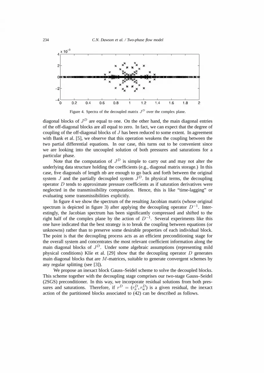
Figure 4. Spectra of the decoupled matrix JD over the complex plane.

diagonal blocks of JD are equal to one. On the other hand, the main diagonal entriesof the off-diagonal blocks are all equal to zero. In fact, we can expect that the degree ofcoupling of the off-diagonal blocks of J has been reduced to some extent. In agreementwith Bank et al. [5], we observe that this operation weakens the coupling between thetwo partial differential equations. In our case, this turns out to be convenient sincewe are looking into the uncoupled solution of both pressures and saturations for aparticular phase.

Note that the computation of JD is simple to carry out and may not alter theunderlying data structure holding the coefficients (e.g., diagonal matrix storage.) In thiscase, five diagonals of length nb are enough to go back and forth between the originalsystem J and the partially decoupled system JD. In physical terms, the decouplingoperator D tends to approximate pressure coefficients as if saturation derivatives wereneglected in the transmissibility computation. Hence, this is like “time-lagging” orevaluating some transmissibilities explicitly.

In figure 4 we show the spectrum of the resulting Jacobian matrix (whose originalspectrum is depicted in figure 3) after applying the decoupling operator D−1. Inter-estingly, the Jacobian spectrum has been significantly compressed and shifted to theright half of the complex plane by the action of D−1. Several experiments like thisone have indicated that the best strategy is to break the coupling between equations (orunknowns) rather than to preserve some desirable properties of each individual block.The point is that the decoupling process acts as an efficient preconditioning stage forthe overall system and concentrates the most relevant coefficient information along themain diagonal blocks of JD. Under some algebraic assumptions (representing mildphysical conditions) Klıe et al. [29] show that the decoupling operator D generatesmain diagonal blocks that are M -matrices, suitable to generate convergent schemes byany regular splitting (see [3]).

We propose an inexact block Gauss–Seidel scheme to solve the decoupled blocks.This scheme together with the decoupling stage comprises our two-stage Gauss–Seidel(2SGS) preconditioner. In this way, we incorporate residual solutions from both pres-sures and saturations. Therefore, if rD = (rDn , rDw ) is a given residual, the inexactaction of the partitioned blocks associated to (42) can be described as follows.


Algorithm 3 (2SGS preconditioner).

1. Solve JDsss = rDw and denote its solution by s.

2. w = rDn − JDpss.

3. Solve JDppp = w and denote its solution by p.

4. Return (p, s ).

Each subsystem is solved iteratively and may in turn be preconditioned by atridiagonal or block-type preconditioner. Clearly, several options can be generateddepending upon the treatment of the subsystems associated with JD . However, theconvergence of the whole procedure depends heavily upon the convergence of eachindividual inner solve. Regarding this as a preconditioner, its efficiency is dictated bythe way in which tolerances are chosen and satisfied for every new outer iteration.

Taking advantage of the above notation, we briefly describe the IMPES type ofapproach proposed by Wallis in his two-stage preconditioner. In this paper, we referto this preconditioner as the two-stage combinative (2SComb) preconditioner after theterminology originally developed by Behie and Vinsome [9].

Given a residual r = (rn, rw) (not previously affected by any decoupled opera-tion), the 2SComb preconditioner can be compactly written as

v = M−12SCombr = M−1[I − (J − M)R(RTJDR)−1

RTD]r. (43)

Here, the M operator represents an extra preconditioning stage that, in practice,should be cheap and aimed at retrieving part of the global information contained in theoriginal Jacobian, J (i.e., M should recover saturation and its coupling informationwith pressures). The reduction operator R is given by R ≡ [Inb×nb0], so it pulls outonly pressure coefficients from JD (i.e., RTJDR ≡ JDpp). In the event of large scaleproblems, Wallis suggests the use of an iterative procedure to obtain pressure solutions.

Note that in opposition to the 2SGS preconditioner, the decoupling here is onlyused as an intermediate step to get pressure solutions. The decoupling is not appliedto J and M . This is one of the main pitfalls of this approach, since it disregards thegood preconditioning effect of the operator D. We refer the reader to [29] for a deeperanalysis on this subject.

Both two-stage preconditioners admit an alternative ordering of the unknowns.That is, we can associate smaller matrix blocks with individual unknowns on the mesh.This formulation can be obtained by interleaving each row and column of pressurecoefficients with each row and column of saturation coefficients. In algebraic terms,this can be done with a permutation matrix. In general, combinative preconditionerapproaches have been presented in this alternate way.

In the event of diagonal dominance for any of the decoupled blocks JDpp and JDss ,the overall cost of both 2SGS and 2SComb preconditioners can be further reducedby the line-correction method proposed by Watts [37]. The basic idea is to add the


residuals in a given direction (collapsing) and solve the reduced problem in a lowerdimension. The solution there should force the sum of the residuals in the removeddirection to be zero. Those solutions are projected back onto the original direction,and then new residuals are formed and corrected by some relaxation steps. Generally,damping is not applied. The collapsing is generally done along the shortest direction(i.e., depth). However, in the case of tilted reservoirs, not assumed here, care must betaken to choose the best direction for collapsing.

We apply the decoupling operator D from the left side of the system (20) and thenapply the block Gauss–Seidel stage as a right preconditioner in order to preserve thenorms already weighted by D throughout the whole globalized HOKN procedure. Theapplication of D−1 requires the use of weighted vector norms. That is, if r = (rn, rw) isa given residual (which concatenates residuals of both the wetting and the nonwettingphases) whose norm needs to be computed then

‖r‖D−1 =∥∥∆−1

∥∥(‖Dssrn −Dpsrw‖2 + ‖−Dsprn +Dpprw‖2)1/2. (44)

Clearly, this does not introduce any major complication or overhead into theimplementation. In fact, an efficient implementation is accomplished by carrying outthe decoupling operation in place over all arrays holding the matrix coefficients. Inorder to restore the original Jacobian coefficients, five arrays are employed to holdthe main diagonal entries of each block and the vector entries of ∆. The coefficientvalues are restored after all Krylov–Broyden steps in the HOKN algorithm have beencompleted, thus allowing use of the same standard Euclidean norm in the line-searchbacktracking strategy, forcing term selection, and in the nonlinear stopping criteria.

Step (44) can also be regarded as a scaling step for the coupled variables of thenonlinear function in a given HOKN step. This scaling improves the robustness of thewhole method. Further discussion on scaling within the Newton method can be seenin [16].

6. Implementation issues

The implementation discussed in this work is based on the Parallel Implicit Ex-perimental Reservoir Simulator (PIERS) code, originally developed by Wheeler andSmith at Exxon [38]. We have made major modifications to the PIERS code, incorpo-rating the full tensor and general boundary condition capabilities, replacing the linearsolver, and adding the line-search procedure. In this section, we discuss some of theimplementation issues involved in these changes, as well as some additional issuesthat have been addressed.

6.1. Time-stepping

In order to ensure rapid convergence of the Newton iteration as well as acceptabletime truncation errors, we define an automatic time step control. If the Newton itera-tion or the backtracking line-search fail to converge within their maximum allowable


number of steps or the Newton iteration did not progress in two consecutive iterations,then the time step is halved and the computation is resumed. Otherwise, the next timestep is set according to a user predefined maximum change of saturations or maximumchange of pressures as

∆tn+1 = ∆tn min

(userSmaxS

,userPmaxP

).

As long as the maximum change in pressure or saturations is not exceeded, we increasethe time step by ∆tn+1 = ∆tnγ, where γ is chosen to be marginally greater than 1.

6.2. Domain decomposition and matrix construction

Our implementation allows for a two-dimensional processor decomposition of thedomain, but no decomposition in the depth direction. Each processor stores data forone subdomain and builds the matrix rows corresponding to its elements. Unknownsare ordered globally by subdomain. Recall that we also have unknowns along the outerboundary corresponding to the multipliers in equation (12). For ease of computation,we introduce extra unknowns along the interfaces between subdomains.

The cell-centered finite difference scheme described above leads to a compactstencil for each unknown. Thus, knowledge of neighboring elements only one cellaway is needed for the calculation of coefficients related to a grid block, and eachprocessor will need to exchange only one cell layer of information with each of itsneighbors. The stencil employed requires information from diagonal neighbors as wellas from the four neighbors sharing sides. Thus, a typical message passing operationinvolves nearest-neighbor exchanges as well as “corner” exchanges. Given currentvalues of the nonwetting phase pressures and saturations, the computation of matrixentries proceeds by first computing physical properties such as wetting phase pressures,relative permeabilities, capillary pressures, etc., exchanging physical properties withneighbors, and then calculating matrix entries corresponding to each grid block. Foreach grid block, the equation corresponding to conservation of the nonwetting phasedepends on 19 pressure unknowns surrounding the block, as shown in figure 1, and 7saturation unknowns. The equation corresponding to the wetting phase depends on the19 pressure unknowns and 19 saturation unknowns. Thus the Jacobian has at most 38nonzero entries per row.

6.3. Parallel implementation of the linear solver

The parallelization of GMRES can be organized in terms of the following com-putational kernels:

• Matrix–vector products.

• Vector updates (AXPYS).

• Inner products.

• Preconditioners.


The sparse matrix–vector multiply (y = βy + αAx) is performed in parallel.Each processor holds the rows of the Jacobian matrix and entries of the vectors x andy corresponding to the grid blocks in that processor’s subdomain. The routine beginswith an exchange of data from neighboring subdomains in order to obtain appropriatevalues of the vector x from neighbors. Each processor then computes its part of thematrix–vector product accumulating each part of the sum corresponding to differentunknown types separately. This separate accumulation is done in order to minimizenumerical error caused by differing sizes in the two types of unknowns. The sums areadded together at the end.

Inner products are computed simply by each processor computing contributionsfrom the relevant vector parts in its memory then participating in a global sum at theend. The AXPY operation does not involve communication of elements.

In the 2SGS preconditioner (algorithm 3), the solution of both pressures and sat-urations is carried out with the GMRES iterative solver. Each GMRES iteration ispreconditioned with a block tridiagonal preconditioner, where the number of blockscorresponds to the number of underlying subdomains (i.e., processors). This precon-ditioner is totally parallel and sufficient to meet the required linear tolerances.

Note that most of the operations in the inner and outer GMRES iterations areparallelizable at the level of BLAS-1 operations (i.e., AXPY’s and inner products). It isalso worth noting that the Krylov–Broyden step in the HOKN method loses a significantpart of parallelism since the Hessenberg matrix is replicated in each processor afterthe Arnoldi process. This is a consequence of partitioning and distributing basisvectors among all processors. Recall that the Hessenberg matrix arises as the resultof performing inner products with vectors on that basis. However, we believe thatblock implementations (i.e., block GMRES [6]) could be favorable in our context anddeserve a separate study.

6.4. Globalization and nonlinear stopping criteria

The major computational component of the backtracking line-search method con-sists of the function evaluation. This function evaluation follows the same steps alreadydescribed in section 6.3. The value of t appearing in equation (28) was set to 0.9999, asis customary in most nonlinear line-search implementations reported in the literature.The maximum number of backtracking steps allowed was set to 10.

The nonlinear stopping criterion is implemented in the following way. Nonlineartolerances are computed locally in every processor i by the following expression,

toli =(totn + totw)

totblocksTOL,

where totl (l = w, n) is the total of phase l produced in the local block, totblocksis the total number of gridpoints in a layer, and TOL is a predefined user tolerance.A global tolerance, tolg, is obtained by computing tolg = min16i6P toli. This tight-ens the convergence to those blocks where major changes in pressure are occurring.The Newton residuals are computed globally in the l2-norm and in agreement to the


norm sizes specified for the line-search backtracking method. Hence, the nonlinearconvergence is achieved whenever ‖F‖ < tolg.

7. Numerical results

In this section we present two test problems and the results of our code appliedto them. The first case is an oil–water problem and the second an air–water problem.

7.1. Oil–water problems

We first discuss the petroleum case. Table 1 summarizes the physical parametersfor this problem, and figure 5 shows the associated relative permeability and capillarypressure functions used. The model consists of a water injection well (with bottomhole pressure specified) located at the coordinate (1, 1) of the plane and a productionwell (with bottom hole pressure specified) at the opposite corner of the plane. Thesize of the domain depends on the number of cells used in the various tests below.

Figure 6 shows the log10 scale plot of the accumulated number of GMRESiterations against the nonlinear residual, ‖F‖, for the oil–water problem. We see thata dynamic strategy for choosing linear tolerances significantly reduces the number

Figure 5. Relative permeability of both phases and capillary pressure.

Table 1Physical input data.

Initial nonwetting phase pressure at 35 ft 600 psiInitial wetting saturation at 35 ft 0.4Nonwetting phase density 48 lb/ft3

Nonwetting phase compressibility 4.2× 10−5 psi−1

Wetting phase compressibility 3.3× 10−6 psi−1

Nonwetting phase viscosity 4.2 cpWetting phase viscosity 0.23 cpAereal permeability 150 mdPermeability along 1st and 2nd half of vertical gridblocks 10 md and 30 md


Figure 6. The use of the forcing term criteria for dynamically controlling linear tolerances. The solidline represents a standard inexact Newton implementation with fixed linear tolerances 0.1. The dotted

line is the inexact Newton implementation with the forcing term criterion.

of GMRES iterations required for the nonlinear convergence. The flat portions ofthe curves show the amount of extra computation needed to decrease the nonlinearresiduals. The problem analyzed here consisted of 18 × 48 × 48 gridblocks on adomain of size 26 × 740 × 740 cubic feet with a non-uniform mesh. The forcingterm criterion decreases tolerances only as the iteration gets closer to convergence andtherefore eliminates the staircase shape given by the standard implementation. In thisparticular example almost 400 GMRES iterations were saved.

In the previous experiment, we used an SP1 machine located at Argonne NationalLab. Each node has the capabilities of an IBM RS/6000-370 workstation with 128Mbytes of RAM memory. For the remaining set of experiments we employed anIBM SP2 machine, located at the University of Texas, Austin. This machine consistsof 16 nodes, each with 128 Mbytes of RAM and it is capable of providing a peakperformance of 260 Mflops and a bidirectional communication rate of 50 MBytes/s.

Table 2 illustrates the performance of GMRES with both the 2SGS preconditionerand the 2SComb preconditioner discussed in section 3.3. We emphasize that traditionalpreconditioners (such as, e.g., block tridiagonal, block Jacobi, ILU) are insufficient inthis scenario of coupled linear systems [29]. The mesh used was 8 × 24 × 24 on adomain of size 13 × 370 × 370 cubic feet.


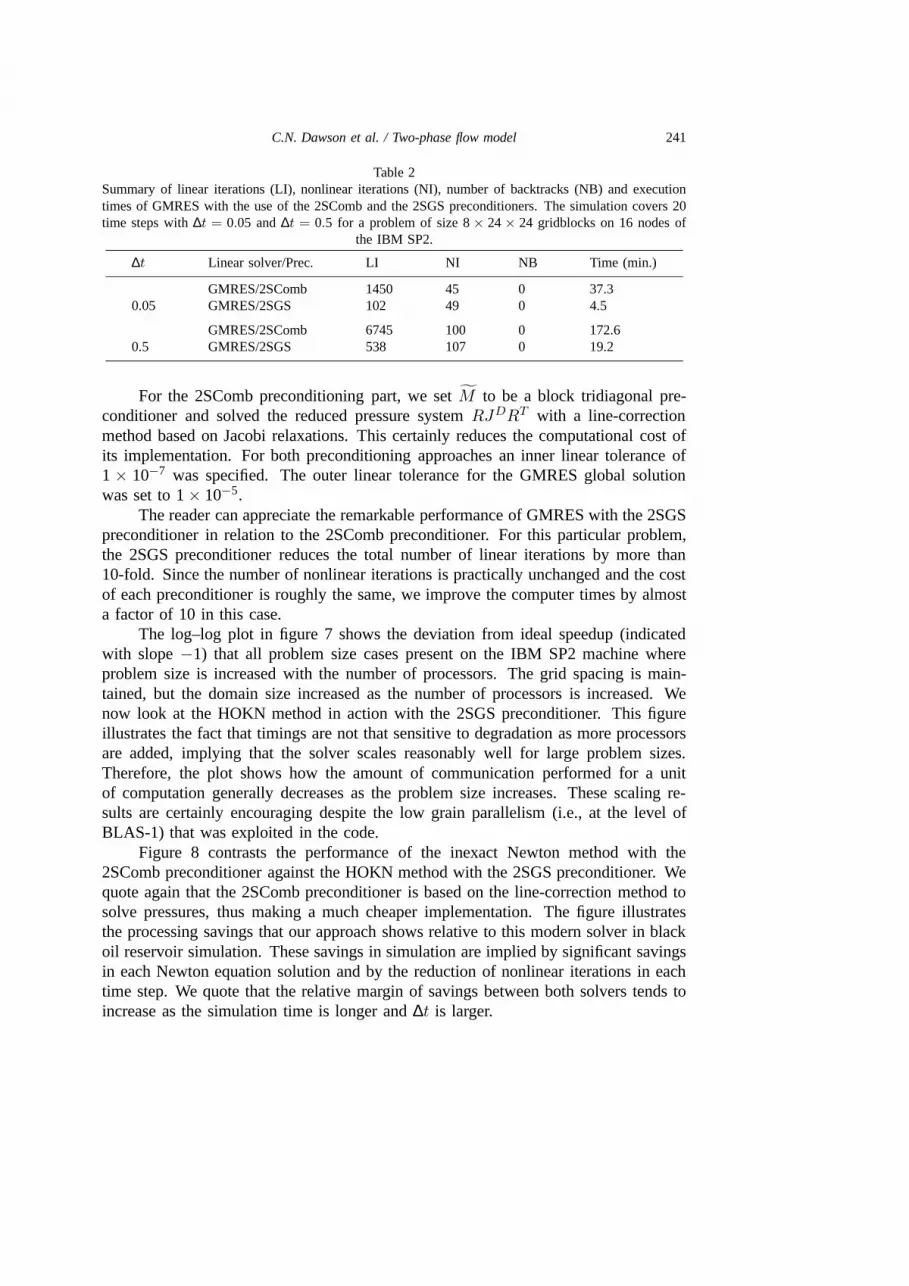
Table 2Summary of linear iterations (LI), nonlinear iterations (NI), number of backtracks (NB) and executiontimes of GMRES with the use of the 2SComb and the 2SGS preconditioners. The simulation covers 20time steps with ∆t = 0.05 and ∆t = 0.5 for a problem of size 8 × 24 × 24 gridblocks on 16 nodes of

the IBM SP2.

∆t Linear solver/Prec. LI NI NB Time (min.)

GMRES/2SComb 1450 45 0 37.30.05 GMRES/2SGS 102 49 0 4.5

GMRES/2SComb 6745 100 0 172.60.5 GMRES/2SGS 538 107 0 19.2

For the 2SComb preconditioning part, we set M to be a block tridiagonal pre-conditioner and solved the reduced pressure system RJDRT with a line-correctionmethod based on Jacobi relaxations. This certainly reduces the computational cost ofits implementation. For both preconditioning approaches an inner linear tolerance of1 × 10−7 was specified. The outer linear tolerance for the GMRES global solutionwas set to 1× 10−5.

The reader can appreciate the remarkable performance of GMRES with the 2SGSpreconditioner in relation to the 2SComb preconditioner. For this particular problem,the 2SGS preconditioner reduces the total number of linear iterations by more than10-fold. Since the number of nonlinear iterations is practically unchanged and the costof each preconditioner is roughly the same, we improve the computer times by almosta factor of 10 in this case.

The log–log plot in figure 7 shows the deviation from ideal speedup (indicatedwith slope −1) that all problem size cases present on the IBM SP2 machine whereproblem size is increased with the number of processors. The grid spacing is main-tained, but the domain size increased as the number of processors is increased. Wenow look at the HOKN method in action with the 2SGS preconditioner. This figureillustrates the fact that timings are not that sensitive to degradation as more processorsare added, implying that the solver scales reasonably well for large problem sizes.Therefore, the plot shows how the amount of communication performed for a unitof computation generally decreases as the problem size increases. These scaling re-sults are certainly encouraging despite the low grain parallelism (i.e., at the level ofBLAS-1) that was exploited in the code.

Figure 8 contrasts the performance of the inexact Newton method with the2SComb preconditioner against the HOKN method with the 2SGS preconditioner. Wequote again that the 2SComb preconditioner is based on the line-correction method tosolve pressures, thus making a much cheaper implementation. The figure illustratesthe processing savings that our approach shows relative to this modern solver in blackoil reservoir simulation. These savings in simulation are implied by significant savingsin each Newton equation solution and by the reduction of nonlinear iterations in eachtime step. We quote that the relative margin of savings between both solvers tends toincrease as the simulation time is longer and ∆t is larger.


Figure 7. Log–log plot of the number of processors vs. execution time for the two-phase problem usingthe HOKN/2SGS solver on an IBM SP2 after 20 time steps.

Table 3CPU time (minutes) of one million and six hundred thousand unknown problems

on 16 nodes of the IBM SP2 for 10 days of simulation with ∆t = 1 day.

Solver 30× 100× 100 50× 100× 100

HOKN/2SGS 50.49 78.24Newton/2SComb 156.26 435.75

In order to show the capabilities of the HOKN/2SGS at large scale we ran sometests representing six hundred thousand and one million unknowns (adding pressureand saturation unknowns). These problem sizes are quite challenging to handle ina fully implicit formulation even for the quasi-homogeneous physical situation (i.e.,moderate changes of permeabilities) modeled here. Nevertheless, a ∆t = 1 day wasspecified to further increase the difficulty of the problem. These results are compiledin table 3.

The HOKN/2SGS solver was able to solve both the six hundred thousand and onemillion unknown cases in approximately 5 and 10 minutes per time step, respectively.An average of roughly 70 linear iterations and 5 nonlinear iterations per time step wereneeded for this short simulation, that is, 15–20 times less accumulated linear iterations


Figure 8. Performance in accumulated CPU time of the HOKN/2SGS and Newton/2SComb solvers after100 time steps of simulation with ∆t = 0.05 of a 16× 48× 48 problem size on 16 IBM SP2 nodes.

than the Newton/2SComb solver. This means that every GMRES solution with the2SGS preconditioner for solving the largest case takes approximately 15 seconds.

It is worth noting that the Newton/2SComb solver required a restart value of 40for each GMRES solution in order to generate acceptable nonlinear directions. Thisturned out to be a serious disadvantage in the largest case run, since paging effectscaused an extra increment in the computing time not shown by the HOKN/2SGSsolver. A restart value of 12 was sufficient to get GMRES convergence with the 2SGSpreconditioner.

7.2. Air–water problems

Table 4 summarizes the physical parameters for the air–water problem. Thisproblem is loosely based on test problem 2 in [22] where the object was to startwith a fairly dry initial condition. Van Genuchten [35] relative permeability andcapillary pressure curves were used with α = 0.085 in−1 and β = 1.982. Figure 9shows the associated relative permeability and capillary pressure functions used. Thecomputational domain was

0 6 x 6 60 ft,

0 6 y 6 60 ft,

0 6 z 6 40 ft,


Table 4Physical input data for the air–water problem.

Initial nonwetting phase pressure at 40 ft 14.7 psiInitial wetting saturation at 40 ft 0.98Residual wetting phase saturation 0.2771Nonwetting phase density 0.076 lb/ft3

Nonwetting phase compressibility 10−5 psi−1

Wetting phase compressibility 3.3× 10−6 psi−1

Nonwetting phase viscosity 0.018 cpWetting phase viscosity 0.23 cpPorosity 0.368Permeability in X-, Y - and Z-directions 9423 mdOff-diagonal permeabilities 1000 md

Figure 9. Relative permeability of air and water phases and the capillary pressure function for theair–water case.

where x is the depth direction. The x direction was divided into 19 cells of 2 feetand 2 cells of 1 foot each. The y and z directions were divided into 80 cells of40× 0.5 foot and 40× 1 foot. Thus, we used 134,400 gridblocks. We applied no flowboundary conditions for both phases on all faces of the domain except the upper facewhere we applied an injection condition. This was accomplished by fixing a constantatmospheric air pressure condition and taking water pressure to be 13 psi in the regionwhere 0 6 y 6 8 ft and 0 6 z 6 8 ft and 8 psi for the rest of the upper face.A gravitational equilibrium calculation was used to determine the initial wetting phasesaturation within the domain. Initial saturations for this problem ranged from 0.98 atthe bottom of the domain to 0.30 at the top. Thus, the upper end of the domain wasstarted at just above residual water saturation.

Table 5 shows total computation times of the air–water problem for both diagonaland full tensor cases on the IBM SP2. For these tests, the nonlinear stopping tolerancewas taken to be 0.2 × 10−3. The simulation was run to one day which took 24time steps. These steps ranged in length from the minimum of 0.001 day to 0.1 day,increasing with time.


Table 5Computation time (hr) summary of the air–water problem on 4, 8,16 and 32 processors with a 21× 40× 40 computational mesh.

Case/Procs. 4 8 16 NL/LI

Diagonal tensor 2.23 1.28 0.81 91/364Full tensor 3.83 2.53 1.45 108/546

The number of nonlinear and linear iterations reported in the last column isfor the 4 processor case. These numbers vary slightly for the 8 and 16 processorcases due to differences in the 2SGS preconditioner as the number of processorschanges. In particular, for the full tensor case these numbers increase slightly to120/626 for 8 processors and 116/604 for 16 processors. The maximum number ofGMRES iterations allowed for each step in the 2SGS preconditioner was 30, and thisnumber was exceeded on several occasions during the simulation. This partly explainsthe suboptimal speed-up factors; however, the speed-up for most runs is still in therange of 1.5–1.8 as the number of processors is doubled.

Lastly, we consider a three-dimensional air–water problem over an irregulargeometry domain. The irregular domain was generated by mapping a rectangulardomain through a C2 map F :R3 → R3. The theory of Arbogast et al. [1] discussesthe transformation of the original problem to one over the rectangular computationaldomain. Specifically, if the mapping is C2, then the problem can be transformed intoan equivalent problem over a rectangular domain which has a convergent solution.The permeability tensor, K, is transformed by,

K = J(DF−1)K(DF−1)T , (45)

where DF is the Jacobian of the map, F , and J is the determinant of DF . Theresulting permeability tensor on the rectangular domain will be full even in the case thatthe original on the irregular domain is diagonal. Furthermore, the time derivative andsource terms are multiplied by J . Applying these transformations allows computationover a regular grid.

Physical data for the irregular domain is the same as that given above for theair–water problem except that we consider the domain

0 6 x 6 20 ft,

0 6 y 6 100 ft,

0 6 z 6 100 ft,

and a larger injection region of 16 ft × 16 ft at the domain top. The domain wasdivided into a 10× 20× 20 computation grid, giving 4000 gridblocks.

Figures 10 and 11 give contour plots of the water saturation after 5 and 15 simu-lation days, respectively. We see that the water moves outward and slowly downwardfrom the injection zone. After 15 days, a significant amount of water has flowed tothe bottom and started to pool at the base of the domain.


Figure 10. Contour plot of water saturation for the irregular domain air–water problem after 5 simulationdays.

Figure 11. Contour plot of water saturation for the irregular domain air–water problem after 15 simulationdays.

8. Conclusions and further work

We have described a fully implicit parallel two-phase flow simulator that incor-porates new advances in the discretization of full tensor permeability problems and inthe solution of large scale nonlinear problems. Our approach consists of an inexacthigher-order Krylov–Newton procedure based on the GMRES iterative method. Inorder to achieve robustness we have implemented a two-stage Gauss–Seidel precon-ditioner based on a simple decoupling strategy that uses two inner GMRES iterationsfor solving the pressure and saturation systems. This inner–outer procedure has beenshown to be effective in handling ill-conditioned linear systems arising from large timesteps or problems with severe physical conditions. We also include a dynamic forcingterm selection as well as line-search globalization for the Newton method. The formerprovides an efficient mechanism to avoid unnecessary linear iterations and the latterincreases the robustness of the Newton method.


We have employed the expanded mixed finite element method in order to simulateheterogeneities present in the physical domain. Furthermore, this method allows forthe modeling of general domain geometries. In order to add flexibility to our numericalmodel we have implemented several types of boundary conditions.

The two-stage preconditioner has been proven to be robust but further work isneeded to accelerate its performance. The authors believe that cheaper and even morerobust preconditioners should be developed for solving both pressures and saturations.A more accurate way of collapsing the problem through line-correction or symmetriza-tion of the resulting decoupled subsystems seems to be an immediate concern. Also,strategies to “freeze” parts of the two-stage preconditioner for several time steps couldbe appealing in combination with polyalgorithmic approaches (see, e.g., [20]).

With respect to the nonlinear iteration, current research is focused on the useof multilevel techniques for solving nonlinear parabolic equations. These techniques,based on the ideas of Xu [40], require the solution of the nonlinear problem on acoarse grid of size H . The problem is then projected to a fine grid of size h H andlinearized about the coarse grid solution. The linear fine grid problem is then solved.This procedure can be repeated for any number of grids where each fine grid problemis like a Newton step for the original nonlinear problem. Asymptotic error estimatesfor this technique applied to cell-centered finite differences for a nonlinear parabolicequation are derived in [15].

Finally, we encourage the use of these ideas for three phases and multicomponentsystems. The inclusion of more features into the simulator will certainly generatefurther insights and enhancements to the model that we have proposed here.

Acknowledgements

The authors wish to thank John Wallis and Homer Walker for their valuableadvice in the implementation of the solver.

References

[1] T. Arbogast, M.F. Wheeler and I. Yotov, Logically rectangular mixed methods for groundwater flowand transport on general geometry, Dept. Comp. Appl. Math. TR94-03, Rice University, Houston,TX (January 1994).

[2] T. Arbogast, M.F. Wheeler and I. Yotov, Mixed finite elements for elliptic problems with tensorcoefficients as cell-centered finite differences, SIAM J. Numer. Anal. 34 (1997) 828–852.

[3] O. Axelsson, Iterative Solution Methods (Cambridge University Press, Cambridge, 1994).[4] K. Aziz and A. Sethari, Petroleum Reservoir Simulation (Applied Science Publisher, 1983).[5] R. Bank, T. Chan, W. Coughran and K. Smith, The alternate-block-factorization procedure for

systems of partial differential equations, BIT 29 (1989) 938–954.[6] R. Barret, M. Berry, T. Chan, J. Demmel, J. Donato, J. Dongarra, V. Eijkhout, R. Pozo, C. Romine

and H. van der Vorst, Templates for the Solution of Linear Systems: Building Blocks for IterativeMethods (SIAM, Philadelphia, PA, 1994).

[7] J. Bear, Dynamics of Fluids in Porous Media (Elsevier, New York, 1972).


[8] G. Behie and P. Forsyth, Incomplete factorization methods for fully implicit simulation of enhancedoil recovery, SIAM J. Sci. Statist. Comput. 5 (1984) 543–561.

[9] G. Behie and P. Vinsome, Block iterative methods for fully implicit reservoir simulation, Soc. ofPetroleum Engineers J. (1982) 658–668.

[10] P. Bjorstad, W.C. Jr. and E. Grosse, Parallel domain decomposition applied to coupled transportequations, in: Seventh International Conference on Domain Decomposition Methods for ScientificComputing, eds. D. Keyes and J. Xu, Como, Italy (American Mathematical Society, 1993).

[11] P.N. Brown, A. Hindmarsh and L. Petzold, Using Krylov methods in the solution of large-scaledifferential–algebraic systems, SIAM J. Sci. Comput. 15 (1994) 1467–1488.

[12] P.N. Brown and Y. Saad, Hybrid Krylov methods for nonlinear systems of equations, SIAM J. Sci.Statist. Comput. 11 (1990) 450–481.

[13] P.N. Brown and Y. Saad, Convergence theory of nonlinear Netwon–Krylov algorithms, SIAM J.Optim. 4 (1994) 297–330.

[14] G. Chavent and J. Jaffre, Mathematical Models and Finite Elements for Reservoir Simulation (North-Holland, Amsterdam, 1986).

[15] C.N. Dawson, M.F. Wheeler and C.S. Woodward, A two-grid finite difference scheme for non-linear parabolic equations, Center for Applied Scientific Computing UCRL-JC-125599, LawrenceLivermore National Laboratory, Livermore, CA (October 1996), to appear in SIAM J. Numer. Anal.

[16] J.E. Dennis and R.B. Schnabel, Numerical Methods for Unconstrained Optimization and NonlinearEquations (Prentice-Hall, Englewood Cliffs, NJ, 1983).

[17] L.J. Durlovsky, Numerical calculation of equivalent grid block permeability tensors for heteroge-neous porous media, Water Resources Research 27 (1991) 699–708.

[18] S. Eisenstat and H. Walker, Globally convergent inexact Newton methods, SIAM J. Optim. 4 (1994)393–422.

[19] S. Eisenstat and H. Walker, Choosing the forcing terms in an inexact Newton method, SIAM J. Sci.Comput. 17 (1996) 16–32.

[20] A. Ern, V. Giovangigli, D. Keyes and M.D. Smooke, Towards polyalgorithmic linear system solversfor nonlinear elliptic problems, SIAM J. Sci. Comput. 15 (1994) 681–703.

[21] R. Ewing, The mathematics of reservoir simulation, in: Frontiers in Applied Mathematics (SIAM,Philadelphia, PA, 1983).

[22] P.A. Forsyth, Y.S. Wu and K. Pruess, Robust numerical methods for saturated-unsaturated flow withdry initial conditions in heterogeneous media, Advances in Water Resources 18 (1995) 25–38.

[23] R.A. Freeze and J.A. Cherry, Groundwater (Prentice-Hall, Englewood Cliffs, NJ, 1979).[24] G. Golub and C. Van Loan, Matrix Computations (Johns Hopkins University Press, Baltimore, MD,

1989).[25] S. Gomez and J. Morales, Performance of Chebyshev iterative method, GMRES and ORTHOMIN

on a set of oil reservoir simulation problems, in: Mathematics for Large Scale Computing (J.C.Diaz, Basel, 1989) pp. 265–295.

[26] T. Kerkhoven and Y. Saad, On acceleration methods for coupled nonlinear elliptic problems, Numer.Math. 60 (1992) 525–548.

[27] H. Klıe, Krylov-secant methods for solving large-scale systems of coupled nonlinear parabolicequations, Ph.D. thesis, Dept. of Computational and Applied Mathematics, Rice University, Houston,TX (September 1996).

[28] H. Klıe, M. Rame and M. Wheeler, Fast Krylov-secant solvers for systems of nonlinear partialdifferential equations, Tech. Rep. TR96-30, Dept. of Computational and Applied Mathematics, RiceUniversity, Houston, TX (1996).

[29] H. Klıe, M. Rame and M. Wheeler, Two-stage preconditioners for inexact Newton methods inmulti-phase reservoir simulation, Tech. Rep. CRPC-TR96641, Center for Research on Parallel Com-putation, Rice University, Houston, TX (1996).


[30] V. Kumar, A. Grama, A. Gupta and G. Karypis, Introduction to Parallel Computing: Design andAnalysis of Algorithms (Benjamin/Cummings, 1994).

[31] C. Mattax and R. Dalton, Reservoir Simulation, SPE Monograph Series 13 (Richardson, TX, 1990).[32] J. Nedelec, Mixed finite elements in R3, Numer. Math. 35 (1980) 315–341.[33] D.W. Peaceman, Fundamentals of Numerical Reservoir Simulation (Elsevier, Amsterdam, 1977).[34] P.A. Raviart and J.M. Thomas, A mixed finite element method for second order elliptic problems,

in: Mathematical Aspects of Finite Element Methods, eds. I. Galligani and E. Magenes, LectureNotes in Mathematics 606 (Springer, Berlin, 1977) pp. 292–315.

[35] M.T. van Genuchten, A closed form equation for predicting the hydraulic conductivity of unsaturatedsoils, Soil Sci. Soc. Amer. J. 44 (1980) 892–898.

[36] J. Wallis, Two-step preconditioning, private communication (1994).[37] J. Watts, A method of improving line succesive overrelaxation in anisotropic problems – a theoretical

analysis, Soc. of Petroleum Engineers J. (1973) 105–118.[38] J. Wheeler and R. Smith, Reservoir simulation on a hypercube, in: 64th Annual Technical Confer-

ence and Exhibition of the Society of Petroleum Engineers, SPE paper No. 19804, San Antonio,TX (1989).

[39] L. Wigton, D. Yu and N. Young, GMRES acceleration of computational fluid dynamics codes, in:Proceedings 1985 AIAA Conference, Denver, CO (1985).

[40] J. Xu, Two-grid discretization techniques for linear and nonlinear PDEs, SIAM J. Numer. Anal. 33(1996) 1759–1777.

A parallel, implicit, cell‐centered method for two‐phase flow with a preconditioned NewtonKrylov...

Documents

Transcript of A parallel, implicit, cell‐centered method for two‐phase flow with a preconditioned NewtonKrylov...