An unstructured Shock-Fitting solver for two-dimensional flows

Renato Paciorri�

, Aldo Bonfiglioli�

�

Dipartimento di Meccanica e Aeronautica, University of Rome, La Sapienza, ItalyE-mail: paciorri@dma.ing.uniroma1.it

�

Dipartimento di Ingegneria e Fisica dell’Ambiente, University of Basilicata, ItalyE-mail: aldo.bonfiglioli@unibas.it

Keywords: Computational Fluid Dynamics, Shock-Fitting, unstructured-grids.

SUMMARY. A new floating Shock-Fitting technique featuring the explicit computation of shocksby means of the Rankine-Hugoniot relations has been implemented on unstructured grids. Thispaper illustrates the algorithmic features of this orginal technique and the results obtained in thecomputation of the hypersonic flow past a circular cylinder and a Mach reflection.

1 INTRODUCTIONShock waves occur very frequently in nature and technological applications. Their presence

characterizes compressible flows not only in aeronautics and aerospace, but also in other areas oftheoretical and applied physics. The extracorporeal shock wave lithotripsy, used for breaking kidneystones, and sonoluminescence, which is the emission of short bursts of light from imploding bubblesin a liquid excited by sound, are two such examples arising in different fields.

In all flows where shock waves occur, these play an important role that affects the overall flowbehavior. We could mention numerous examples testifying the importance of shock waves and theireffects. Among these are: the flow around space vehicles re-entering the atmosphere at hypersonicspeeds, the buffeting phenomenon induced by oscillating shock waves on transonic wings and tur-bomachinery blades, shock-induced noise and shock-induced boundary-layer separation that occursinside highly over-expanded nozzles. It is therefore not surprising that computing shocks correctlyhas always been one of the most important issues in the numerical simulation of compressible flows.

The numerical models used in the simulation of compressible flows can be cast into two maincategories: Shock-Capturing (S-C) and Shock-Fitting (S-F).

The technique for compressible flow computations known as S-F was proposed and developedby Gino Moretti [Moretti and Abbett, 1966, Moretti, 1987].

It consists in finding the precise shock location and computing the shock motion by means ofthe Rankine-Hugoniot (R-H) equations. Besides Moretti, other researchers applied this techniquein the seventies and eighties [Salas, 1976, Marconi and Salas, 1973, Yamamoto et al., 1984] and inthe early nineties [Hartwich, 1990, Dadone and Fortunato, 1994]. In those years, the S-F technique,used in conjunction with numerical schemes based on the quasi-linear equations, allowed to accu-rately compute flows with strong discontinuities using the modest computational resources availableat that time. In the nineties, however, the development of modern S-C schemes based on the integralconservation equations along with the strong growth in computing resources diminished the interestin S-F schemes, which were considered too complex and not general enough as compared to S-Cschemes. The development and the application of the S-F technique was pursued with good resultsby only one research team [Nasuti and Onofri, 1998].

Despite the widespread use of S-C codes, shock solutions obtained by means of S-C schemes areplagued by a number of problems pertaining to accuracy [Lee and Zhong, 1999, Carpenter and Casper, 1999,

1

Roy, 2003], stability [Pandolfi and D’Ambrosio, 2001] and, more in general, solution quality. De-spite the continuous efforts made over the last 20 years, these shortcomings have not been completelyovercome and appear to be particulary severe when unstructured-grids are used [Gnoffo and White, 2004].

The S-F technique, on the contrary, does not suffer from these numerical problems but, as it wassaid before, it has been abandoned over the last decades. We believe there exist today good reasonsfor reconsidering the S-F technique in the context of unstructured grids.

During their historical development, Computational Fluid Dynamics (CFD) techniques have firstbeen developed to use structured grids. Compared to unstructured-grid methods, the former offera number of advantages, most notably a reduced algorithmic complexity which results in improvedcomputational efficiency. Nevertheless, starting in the early nineties, the CFD community has shownan increasing interest in unstructured-grid techniques. This is mainly due to the following features,which are peculiar to unstructured grids: i) the ability to describe complex geometries and ii) thepossibility of locally adapting the grid to follow the flow features. This latter capability makes themparticularly well suited to simulate compressible flows, which may develop discontinuities such asshock waves and contact discontinuities.

Moretti’s S-F technique was born at a time when CFD practitioners used solvers based only onstructured meshes. The algorithmic complexity and the difficulties encountered in the implemen-tation of the S-F methodology within structured-grid solvers has been one of the main reasons forthe loss of interest in S-F. In the traditional implementation of the S-F technique, the discontinuitiesare made up of shock points connected by shock segments which move over and independently ofthe background structured grid. Moreover, new shock points may arise or disappear when shocksinteract or weaken into Mach lines or when compression waves coalesce into a new shock. Thealgorithmic tools that can most effectively handle the motion of the shocks, their intersections, etc.are far from the IJK data structures used in structured-grid methods. On the contrary, the unstruc-tured grid technology appears to be much better suited to handle the motion, insertion and removalof shock points as well as the local re-meshing that is required when the discontinuities move over abackground mesh.

To our knowledge, only a few attempts have been made to incorporate S-F ideas within S-Cunstructured-grid solvers. These include the work by Van Rosendale [Rosendale, 1994], Parpiaand Parikh [Parpia and Parikh, 1994], Trepanier [Trepanier et al., 1996] and co-workers and, morerecently, Hanel [Gloth et al., 2003] and co-workers.

The strategies adopted in [Rosendale, 1994, Parpia and Parikh, 1994, Trepanier et al., 1996] aresimilar: rather than explicitly solving the R-H relations to compute the shock, use is made of theproperty of Roe’s approximate Riemann solver [Roe, 1981] to return the exact jump relations whenthe discontinuity is aligned with the mesh. Therefore, all three methods try to locally align the edgesof the triangulation with the discontinuities by means of grid motion and/or adaptation.

On the contrary, in [Gloth et al., 2003] the grid is stationary and made of arbitrary polygonal ele-ments. The shock motion is computed using a level-set method. The local shock speed is computedby solving the R-H equations with values on both sides of the discontinuity obtained by one-sidedextrapolation. A special treatment is also required to compute the flux integrals in those cells thatare crossed by the shock front.

The present paper tries to revive Moretti’s original floating S-F technique by formulating it asa local adaption algorithm on unstructured triangular grids and coupling it with an unstructured,vertex-centred, S-C code. The use of a S-C code, rather than a solver based on the quasi-linear equa-tions, as was tipically done in the traditional S-F implementation, allows to use an hybrid techniquein which, for example, the strongest shock is fitted and the other shocks are captured. This could be

2

advantageous particularly in the three dimensional case, where fitting interacting shocks might behard to handle analitically.

In the proposed approach, the shock front is discretized as a polygonal curve and treated as aninternal boundary for the CFD code: its local speed and downstream nodal values are computedby coupling the upstream moving wave predicted by the S-C code with the R-H relations. Thediscontinutity is allowed to move over and independently of a background triangular grid which islocally adapted to ensure that the edges of the shock are part of a constrained Delaunay triangulation(CDT) that covers the entire computational domain.

Results are persented for the bow shock that is formed ahead of a circular cylinder moving athypersonic speed and a Mach reflection.

2 SHOCK FITTING ALGORITHMThe present S-F algorithm is able to compute single shocks occurring within a two-dimensional

flow field discretized by an unstructured mesh made of triangles. In its current version, the algorithmdoes not include any procedure for shock detection. Therefore, the fitted shocks must be presentwithin the flow domain at the beginning of the simulation.

In order to illustrate the algorithmic features of the proposed methodology, let us consider a two-dimensional domain and a shock front crossing this domain at time level

�, see Fig. 1a). The shock

front is shown in bold by a polyline whose endpoints are the shock points, marked by squares. Abackground triangular mesh, whose nodes are denoted by circles, covers the entire computationaldomain and the position of the shock points is completely independent of the location of the nodesof the background grid. While each node of the background mesh is characterized by a single setof state variables, two sets of values, corresponding to the upstream and downstream states, areassigned to each shock point.

We assume that at time�

the solution is known in all grid and shock points. The computation ofthe subsequent time level

�������can be split into several steps that will be described in detail in the

following sub-sections.

phantom nodes

Cells crossed by shock

Phantomnodes

Cells enclosing

d l

Upstream

Shock

DownstreamDownstream

n

τ

shock

Upstream

n

τ

a) b)

Figure 1: a) shock front moving over the background triangular mesh at time�: dashed lines mark

the cells to be removed; dashed circles denote the phantom nodes; b) the triangulation around theshock has been rebuilt.

3

2.1 Cell removal around the shock frontThe first step consists in removing the cells around the shock front. More precisely, all cells of

the background mesh that are crossed by the shock line are removed along with the mesh pointswhich are located too close to the shock front. These nodes are declared as “phantom” nodes and allcells having at least one phantom node among their vertices are also removed from the backgroundtriangulation, see dashed circles and cells in Fig. 1a).

2.2 Local re-meshing around the shock frontFollowing the cell removal step, the remaining part of the background mesh is split into two

regions separated by a hole containing the shock. The hole is then re-meshed using a CDT: both theshock segments and the edges belonging to the boundary of the hole are constrained to be part of thefinal triangulation, see Fig. 1b). No further mesh point is added during this triangulation process.At this stage, the computational domain is discretized by a modified mesh in which the shock pointsand the shock edges are part of the triangulation. This mesh differs from the background mesh onlyin the neighbourhood of the shock front.

2.3 Computation of the tangent and normal unit vectorsThe tangent and normal unit vectors along the shock front have to be computed in each shock

point since this is required to properly compute the jump relations, see Fig. 1b). The computation ofthese vectors in a generic shock point is carried out through specific finite-difference formulas whichinvolve the coordinates of the shock point itself and of its neighbouring shock points belonging toits domain of dependence.

2.4 Solution update using the capturing codeThe solution is updated at time level

� � � �using the unstructured, S-C code and the modified

mesh as input. The modified mesh is split into two non-communicating parts by the shock frontwhich is treated by the code as if it were an internal boundary, see Fig. 2a). This is achieved byreplacing each shock point by two superimposed mesh points: one belonging to the downstream re-gion and the other to the upstream region. The downstream and upstream states are correspondinglyassigned to each pair of shock nodes. A single time step calculation is performed by the unstructuredsolver which provides updated nodal values within all grid and shock points at time level

� � � �.

However, the downstream state of the shock points has not been correctly computed except for thefollowing combination of variables:

��������� �� ������� �� �������������� ��� (1)

where � is the shock normal, �������� and �

������� are the values of the acoustic and flow velocity ofthe downstream state of the shock nodes computed by the unstructured solver.

2.5 Shock calculationEach shock point is characterized by an upstream state, a downstream state and a shock speed,

� . The upstream state has been updated at time level� � � �

in the previous step 2.4. Concerningthe downstream state, only the quantity

� has been correctly updated. The complete downstreamstate and the shock speed are computed through a system of five algebraic equations where fourequations are the R-H relations written with respect to the shock point moving at the unknown speed

4

Upstreamstate

Downstream state

Shockpoint

Phantomnode

Cell containgthe phantom node

a) b)

Figure 2: a) the shock is treated as an internal boundary; b) interpolation of the phantom nodes.

� . Finally, the last equation of the system is the variable combination of Eq.1 where the value�

has been computed in the previous step 2.4.

2.6 Interpolation of the phantom nodesIn the previous steps all nodes of the modified mesh have been updated at time level

� � � �.

Nevertheless the phantom nodes, which belong to the background mesh but had been excluded fromthe modified mesh, have not been updated, see Fig. 2b).

The update of the phantom nodes is performed by first locating each of these within the modifiedmesh (a search operation which can be efficiently performed on a Delaunay mesh) and then usinglinear interpolation.

2.7 Shock displacementThe new position of each shock point at time

� � ���is computed using the shock speed calculated

in the previous step 2.5 by the following first order integration formula:

� ������� � � � � ������� � � ��� (2)

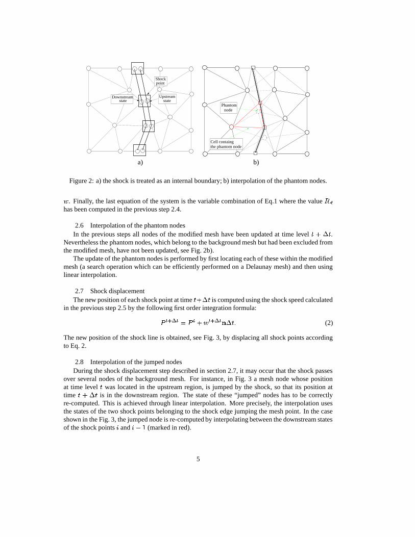
The new position of the shock line is obtained, see Fig. 3, by displacing all shock points accordingto Eq. 2.

2.8 Interpolation of the jumped nodesDuring the shock displacement step described in section 2.7, it may occur that the shock passes

over several nodes of the background mesh. For instance, in Fig. 3 a mesh node whose positionat time level

�was located in the upstream region, is jumped by the shock, so that its position at

time� � � �

is in the downstream region. The state of these “jumped” nodes has to be correctlyre-computed. This is achieved through linear interpolation. More precisely, the interpolation usesthe states of the two shock points belonging to the shock edge jumping the mesh point. In the caseshown in the Fig. 3, the jumped node is re-computed by interpolating between the downstream statesof the shock points � and � � � (marked in red).

5

t+ t∆

t+ t∆ιPt+ t∆

Pt

ι+1 Pι+1

Pιt

jumped node

jumping edge

A

ιw n t∆

Figure 3: Mesh points jumped by the shock and their re-computation.

3 UNSTRUCTURED SOLVERAs described in section 2, the proposed S-F algorithm provides a time dependent mesh in which

the discontinuity is treated as an internal boundary of zero thickness. Communications with theCFD code are only required in step 2.4, when the modified grid containing the shock front is fedto the code which returns provisional values of the nodal variables at the subsequent time level.This reduced amount of communication allows to treat the CFD code as a black box, thus makingthe proposed S-F algorithm re-usable in conjunction with virtually any vertex-centred unstructuredCFD code. It is however worth briefly describing the EULFS solver used to produce the numericalresults presented in Sect. 4. A more detailed description can be found in [Bonfiglioli, 2000].

In the testcases presented in Sect. 4, which are restricted to two spatial dimensions, the govern-ing conservation laws are the Euler equations for a non-viscous, non-conducting, perfect gas. Thecomputational domain is partitioned into a set of non-overlapping triangular cells. Roe’s parametervector [Roe, 1981] is chosen as dependent variable: it is stored in the vertices of the mesh and as-sumed to vary linearly and continuously in space, just as with iso-P1 linear Finite Elements (FE).The control volumes over which the system of conservation laws is discretized are the median dualcells.

To enhance accuracy, the Euler equations are solved in preconditioned form, using the vanLeer,Lee, Roe matrix [van Leer et al., 1991]. This approach is often referred to as the Hyperbolic-Elliptic(HE) splitting as it allows to achieve full or partial (depending on the flow regime) diagonalisation ofthe original unsteady Euler system. In supersonic flows, this is re-cast into a set of four scalar equa-tions describing convection of entropy and total enthalpy along the streamlines and convection ofthe acoustic variables along the Mach lines. In subsonic flows, the acoustic component is describedby a coupled 2 � 2 Cauchy-Riemann system, while entropy and total enthalpy are convected alongthe streamlines, just as in supersonic flows.

The spatial discretization relies upon the so-called Residual Distribution (RD) (or fluctuationsplitting) schemes [Deconinck et al., 1993a] which share common features with both FE and FiniteVolume (FV) techniques. RD schemes operate by evaluating the flux integrals (or cell residuals) overeach triangular cell and distributing them among the forming vertices. The nodal residual, which isdriven to zero as steady state is approached, is obtained by assembling the fractions of cell residualsscattered from the elements surrounding the node. A distinctive feature adopted in many RD codesis that the flux balance over a triangular cell in not computed using numerical quadrature, but using

6

the quasi-linear form of the equations and a multi-dimensional generalisation of Roe’s linearisation[Deconinck et al., 1993b]. Contrary to most FV schemes, no Riemann problems are involved inRD schemes since the functional representation of the dependent variables is continuous across theelements. The discretization of the viscous fluxes can be shown to be equivalent to a standard FE dis-cretization, while the inviscid fluxes are distributed in an upwind-biased fashion. These upwindingdirections are based upon the eigenstructure of the quasi-linear form of the equations, as describedin details in [Bonfiglioli, 2000].

Concerning time integration, a simple Euler explicit scheme has been used and mass lumpingapplied to the time derivative term.

4 APPLICATIONS4.1 Blunt body problem

The first test case deals with the high speed flow past a circular cylinder at free-stream Machnumber,

��� ���. This and similar testcases have been used by other authors to assess the

accuracy of high order S-C schemes within a structured grid setting. It has been observed in[Lee and Zhong, 1999, Carpenter and Casper, 1999, Roy, 2003] that, when captured shock wavesare present, the order of accuracy of the computed solution downstream of the shock wave is re-duced below the design order of the scheme, tipically to first order only. This is due to the fact thatthe high order scheme needs to be reduced to a first order scheme across the shock wave to capturethe discontinuity without oscillations. The result is that the numerical solution is just first-order ac-curate downstream of the discontinuity, regardless of the design accuracy of the discretization used.In a S-F code this is not an issue since the discontinuity is explicitly computed by means of the R-Hequations and elsewhere the flow is smooth so that higher order schemes can be used everywhere.

The present calculations have been performed using the EULFS code both in S-C and S-F mode.

Table 1: Nodes and cells of the background and modified meshes.

level Background Initial Final modifiedmesh shock mesh

cells nodes nodes cells nodes shocknodes

coarse 610 351 29 624 358 29fine 2544 1365 61 2580 1383 57

Two grids of increasing spatial resolution (see Tab. 1) have been created by specifying the dis-tribution of the boundary nodes. These are evenly spaced and the distance between two adjacentboundary nodes of the coarse mesh equals R/12.5, R being the radius of the circular cylinder.

The fine mesh is obtained by halving the distance between two adjacent boundary nodes andremeshing the interior of the computational domain. For this reason the number of cells and back-ground grid nodes is approximately four times that of the coarse mesh, whereas the number of shockpoints is nearly twice.

Different RD schemes have been selected when the code was used in S-C and S-F mode. Inboth cases, the entropy and total enthalpy scalar convection equations were discretized using thenon-linear, monotone and second-order accurate, scalar PSI scheme. Concerning the two scalarequations describing convection along the Mach lines in supersonic regions and the 2 � 2 Cauchy-Riemann system in subsonic regions, different schemes have been used in capturing and fitting mode.

7

For the S-F solutions, the linear, second order accurate, and therefore not necessarily monotonicity-preserving, system LDA scheme, could be used since the shock is fitted and the flow-field is smoothelsewhere. In the S-C solutions, a non-linear system scheme (B scheme) has been used which is ablending of two linear system schemes: the first order, monotone N scheme and the system LDAscheme. Non-linearity is brought into the scheme by the blending function [Abgrall, 2001] which isable to switch between the N scheme in the neighbourhood of a discontinuity and the LDA schemein smooth regions of the flow field.

The solution computed by the unstructured code in S-C mode was used to initialize the flow-fieldand to determine the initial position of the shock front. In the S-F simulation, the initial upstreamstate in the shock points is set equal to the freestream conditions, while the initial downstream stateis computed from the upstream state and the shock slope assuming zero shock speed. The coarsebackground mesh is made of 351 nodes and 29 shock points are preset at the beginning of thesimulation. Afterwards, the flow-field and the shock position are integrated in time until steady stateis reached. During the computation the number of nodes of the modified mesh may vary with respectto that of the background mesh. Indeed, the modified mesh used in the last time iteration is madeof 358 gridpoints, 29 of which are shock points. The re-meshing technique does not significantlyincrease the number of points and cells with respect to the background mesh, since the addition ofthe shock nodes in the modified mesh is partly balanced by the removal of the phantom nodes.

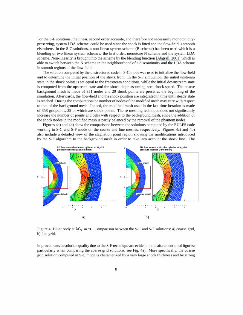
Figures 4a) and 4b) show the comparisons between the solutions computed by the EULFS codeworking in S-C and S-F mode on the coarse and fine meshes, respectively. Figures 4a) and 4b)also include a detailed view of the stagnation point region showing the modifications introducedby the S-F algorithm to the background mesh in order to take into account the shock line. The

X

Y

0 1 2 3 4 5 6

-2

-1

0

1

2

3

fitted shock

captured shock

2D flow around a circular cylinder at M∞=20pressure isolines (Coarse mesh)

X

Y

0.5 1 1.5 2 2.5

-1

-0.5

0

0.5

1

X

Y

0 1 2 3 4 5 6

-2

-1

0

1

2

3

fitted shock

captured shock

2D flow around a circular cylinder at M∞=20pressure isolines (Fine mesh)

X

Y

0.5 1 1.5 2 2.5

-1

-0.5

0

0.5

1

a) b)

Figure 4: Blunt body at� � � � . Comparison between the S-C and S-F solutions: a) coarse grid,

b) fine grid.

improvements in solution quality due to the S-F technique are evident in the aforementioned figures;particularly when comparing the coarse grid solutions, see Fig. 4a). More specifically, the coarsegrid solution computed in S-C mode is characterized by a very large shock thickness and by strong

8

spurious disturbances affecting the shock layer region. These disturbances originate from the shockand are caused by the mis-alignment between the mesh and the shock. On the contrary, the S-Fsolution shows a very neat field. As far as the fine grid solutions are concerned, see Fig. 4b), theone computed in S-F mode appears to be very similar to that obtained on the corse mesh, whereasthe S-C solution still shows the presence of spurious oscillation even if the shock thickness has beenhalved. Also in this case, the S-F solution shows a significant gain in terms of solution qualitywith respect the S-C solution. Of course, the resolution of the S-C solutions could be significantlyimproved if local grid-refinement were used in the shock region, see e.g. [Gnoffo and White, 2004].However, the results presented in [Yamaleev and Carpenter, 2002] seem to indicate that even gridredistribution and local grid refinement do not significantly improve the numerical solution accuracycompared to that obtained on a uniform grid.

A quantitative analysis of the S-F solutions was carried out by comparing the estimates of theshock position and the pressure distribution computed on both grid levels with the reference solutioncomputed by [Lyubimov and Rusanov, 1973]. In Figures 5a) and 5b) the distance (

�����) between the

shock and the cylinder wall and the normalized pressure at the wall are plotted against the azimuthalangle ( � ). This analysis clearly proves that the coarse grid solution is grid-independent despite theextremely limited number of cells enclosed in the shock layer. A comparison between the S-F and the

Θ

d sh

0 30 60 900

0.2

0.4

0.6

0.8

1

1.2

1.4

CoarseFineLyubimov et al.

X

Y

0 1 2 30

1

2

Θd sh

Θ

p/p

∞

0 30 60 900

100

200

300

400

500

CoarseFineLyubimov et al.

a) b)

Figure 5: Blunt body at��� � � . Comparison between the S-F and reference solutions: a) shock-

wall distance, b) normalized pressure at wall

S-C solutions is displayed in Fig. 6 where the normalized pressure distributions along the line at 45degrees is plotted. The S-C solutions are characterized by a finite shock thickness that significantlyaffects the distribution even on the fine grid. Nevertheless, significant differences between the S-Csolutions and the reference one are also visible in regions far from the shock. On the contrary, thedifferences between the shock fitting solutions and the reference one are very small and the fine gridsolution is nearly superimposed to the reference one.

9

4.2 Mach reflectionThe second test-case deals with the Mach reflection that occurs when a uniform flow at

� � � ��� is deflected by an agle of � � ��� degrees. This case gives the opportunity to verify the hybridsolution technique in which some of the shock are fitted while others are captured. Three solutionshave been computed by: i) capturing all shocks, ii) fitting all shocks, iii) capturing the incidentshocks and fitting the reflected shock and the Mach stem. In all cases the contact discontinuity hasnot been fitted, but captured. Concerning the RD schemes used for the spatial discretisation, theentropy and total enthalpy transport equations have been discretized using the PSI scheme, while thesystem B scheme has been used for the remaining two equations. All three solutions are displayedin Figure 7, which focuses on the Mach stem region. Observe, in particular, that fitting the Machstem removes the oscillations that are observed in the subsonic region downstream of the capturedMach stem (top of Figure 7a).

5 CONCLUSIONSWe believe to have shown that fourty years [Moretti, 2002] after it was first proposed, Moretti’s

S-F technique can still be effectively used to accurately compute flows with shocks on relativelycoarse meshes. Its use in conjunction with unstructured grids, which is the original contributionproposed in the present paper, allows to overcome many of the algorithmic difficulties that havecontributed to the demise of S-F algorithms over the last decades. The use of a S-C code to computethe smooth regions of the flow provides additional flexibility in the sense that it allows to use anhybrid technique in which some of the shocks are fitted while others are captured. This could be anuseful feature for extending the methodology to three spatial dimensions.

References[Abgrall, 2001] Abgrall, R. (2001). Towards the Ultimate Conservative Scheme: Following the

Quest. Journal of Computational Physics, 167(2):277–315.

[Bonfiglioli, 2000] Bonfiglioli, A. (2000). Fluctuation splitting schemes for the compressible andincompressible Euler and Navier-Stokes equations. Int. J. Computational Fluid Dynamics, 14:21–39.

[Carpenter and Casper, 1999] Carpenter, M. H. and Casper, J. H. (1999). Accuracy of Shock Cap-turing in Two Spatial Dimensions. AIAA Journal, 37(9):1072–1079.

[Dadone and Fortunato, 1994] Dadone, A. and Fortunato, B. (1994). Three-dimensional flow com-putations with shock fitting. Comp. and Fluids, 23:539–50.

[Deconinck et al., 1993a] Deconinck, H., Paillere, H., Struijs, R., and Roe, P. (1993a). Multidimen-sional upwind schemes based on fluctuation-splitting for systems of conservation laws. Compu-tational Mechanics, 11(5/6):323–340.

[Deconinck et al., 1993b] Deconinck, H., Roe, P., and Struijs, R. (1993b). A Multi-dimensionalGeneralization of Roe’s Flux Difference Splitter for the Euler Equations. Journal of Computersand Fluids, 22(2/3):215–222.

[Gloth et al., 2003] Gloth, O., Hanel, D., Tran, L., and Vilsmeier, R. (2003). A front trackingmethod on unstructured grids. Comp. & Fluids, 32:547–570.

[Gnoffo and White, 2004] Gnoffo, P. and White, J. A. (2004). Computational AerothermodynamicSimulation Issues on Unstructured Grids. AIAA-CP-2004-2371.

[Hartwich, 1990] Hartwich, P. M. (1990). Fresh look at floating shock fitting. AIAA J., 29:1084–91.

[Lee and Zhong, 1999] Lee, T. K. and Zhong, X. (1999). Spurious numerical oscillations in simu-lation of supersonic flows using shock-capturing schemes. AIAA Journal, 37(3):313–319.

10

[Lyubimov and Rusanov, 1973] Lyubimov, A. N. and Rusanov, V. V. (1973). Gas flows past bluntbodies, part ii, table of the gasdynamic functions. NASA TT F-715.

[Marconi and Salas, 1973] Marconi, F. and Salas, M. (1973). Computation of three dimensionalflows about aircraft configurations. Comp. & Fluids, 1:185–195.

[Moretti, 1987] Moretti, G. (1987). Computation of flows with shocks. Ann. Rev. Fluid Mechanics,19:313–7.

[Moretti, 2002] Moretti, G. (2002). Thirty-six years of shock fitting. Computers and Fluids,31:719–723(5).

[Moretti and Abbett, 1966] Moretti, G. and Abbett, M. (1966). A time-dependent computationalmethod for blunt body flows. AIAA J., 4:2136–41.

[Nasuti and Onofri, 1998] Nasuti, F. and Onofri, M. (1998). Viscous and inviscid vortex generationduring startup of rocket nozzles. AIAA J., 36:809–15.

[Pandolfi and D’Ambrosio, 2001] Pandolfi, M. and D’Ambrosio, D. (2001). Numerical Instabilitiesin Upwind Methods: Analysis and Cures for the ”Carbuncle” Phenomenon. Journal of Compu-tational Physics, 166(2):271–301.

[Parpia and Parikh, 1994] Parpia, I. H. and Parikh, P. (1994). A solution-adaptive mesh generationmethod with cell-face orientation control. In AIAA, Aerospace Sciences Meeting and Exhibit,32nd, Reno, NV; UNITED STATES; 10-13 Jan., number AIAA-1994-416.

[Roe, 1981] Roe, P. L. (1981). Approximate riemann solvers, parameter vectors and differenceschemes. J. of Comp. Physics, 43:357–372.

[Rosendale, 1994] Rosendale, J. V. (1994). Floating shock fitting via lagrangian adaptive meshes.Technical report, Institute for Computer Applications in Science and Engineering, NASA LangleyResearch Center, Hampton, VA 23681-0001. NASA Contractor Report 194997; ICASE ReportNo. 94-89.

[Roy, 2003] Roy, C. J. (2003). Grid Convergence Error Analysis for Mixed-Order NumericalSchemes. AIAA Journal, 41(4):595–604.

[Salas, 1976] Salas, M. D. (1976). Shock fitting method for complicated two-dimensional super-sonic flows. AIAA J., 14:583–8.

[Trepanier et al., 1996] Trepanier, J.-Y., Paraschivoiu, M., Reggio, M., and Camarero, R. (1996). Aconservative shock fitting method on unstructured grids. J. comp. Physics, 126:421–433.

[van Leer et al., 1991] van Leer, B., Lee, W.-T., and Roe, P. (1991). Characteristic Time-Steppingor Local Preconditioning of the Euler equations. In AIAA 10th Computational Fluid DynamicsConference. AIAA-91-1552-CP.

[Yamaleev and Carpenter, 2002] Yamaleev, N. K. and Carpenter, M. H. (2002). On accuracy ofadaptive grid methods for captured shocks. J. Comput. Phys., 181(1):280–316.

[Yamamoto et al., 1984] Yamamoto, O., Anderson, D. A., and Salas, M. (1984). Numerical calcu-lations of complex mach reflection. Technical Report 84–1976.

11

r

p/p

∞

1 1.2 1.4 1.6 1.80

100

200

300

400

Ref. [6]S-C coarseS-C fineS-F coarseS-F fine

shockbody

X

Y

0 1 20

1

2

3

45°

r

shock

body

Figure 6: Blunt body at� � � � . Normalized pressure along the 45 degrees line: comparison

among the computed solutions and the reference solution.

X

Y

1 1.5 2

1.25

1.5

1.75

2

2.25

2.5

2.75

All shocksare captured

All shocksare fitted

M = 1.5

Iso-Mach contours

X

Y

1 1.5 2

1.25

1.5

1.75

2

2.25

2.5

2.75

The incident shockis captured; all othershocks are fitted

All shocksare fitted

M = 1.5

Iso-Mach contours

a) b)

Figure 7: Mach reflection with� � � � � and � � ��� : detail of the Mach stem region.

12