Shock interaction computations on unstructured, two-dimensional grids using a shock-fitting...

Journal of Computational Physics 230 (2011) 3155–3177

Contents lists available at ScienceDirect

Journal of Computational Physics

journal homepage: www.elsevier .com/locate / jcp

Shock interaction computations on unstructured, two-dimensionalgrids using a shock-fitting technique

Renato Paciorri a, Aldo Bonfiglioli b,⇑a Dipartimento di Ingegneria Meccanica e Aerospaziale, Universitá di Roma, La Sapienza, Via Eudossiana 18, 00184 Roma, Italyb Dipartimento di Ingegneria e Fisica dell’Ambiente, Universitá della Basilicata, Viale dell’Ateneo Lucano 10, 85100 Potenza, Italy

a r t i c l e i n f o a b s t r a c t

Article history:Received 12 August 2010Received in revised form 22 December 2010Accepted 10 January 2011Available online 14 January 2011

Keywords:Shock-fittingUnstructured-gridsShock interactions

0021-9991/$ - see front matter � 2011 Elsevier Incdoi:10.1016/j.jcp.2011.01.018

⇑ Corresponding author.E-mail addresses: [email protected]

A new shock-fitting technique has been recently proposed and implemented by theauthors in conjunction with an unstructured shock-capturing solver. In the present paper,the attention is addressed towards the computation of shock–shock and shock–wall inter-actions by means of this novel computational technique.

� 2011 Elsevier Inc. All rights reserved.

1. Introduction

A recent book [1] authored by Salas may eventually renew the interest of the CFD community in shock-fitting, a numericaltechnique for computing compressible flows with shocks that has enjoyed a remarkable popularity at the dawn of compu-tational fluid dynamics, but has nowadays been almost completely abandoned in favour of the shock-capturing approach.

Shock-fitting consists in locating and tracking the motion of the discontinuities which are treated as boundaries betweenregions where a smooth solution to the governing PDEs exists. The appropriate jump relations (algebraic equations connect-ing the states on either side of the discontinuity and its local speed) are used to calculate the space–time evolution of thediscontinuity.

Shock-capturing discretisations, on the contrary, rely on the proven mathematical legitimacy of weak solutions, whichallow to compute all type of flows, including those with shocks, using the same discretisation of the conservation law formof the governing equations at all grid points.

Therefore, contrary to shock-fitting, shock-capturing schemes are able to provide solutions featuring physically meaning-ful shocks without requiring any special treatment to deal with discontinuities. This has obvious consequences in terms ofcoding simplicity, since the same set of operations is repeated within all grid-points in the mesh, no matter how complicatedthe flow might be.

Coding simplicity is the primary reason for the widespread use of shock-capturing schemes in the simulation of com-pressible flows with shock waves.

Coding simplicity comes not for free, however. Indeed, shock capturing schemes often incur numerical problems thatcompromise the solution quality. We shall now give a brief account of at least some of these drawbacks.

. All rights reserved.

(R. Paciorri), [email protected] (A. Bonfiglioli).

http://dx.doi.org/10.1016/j.jcp.2011.01.018

mailto:[email protected]

mailto:[email protected]


http://www.sciencedirect.com/science/journal/00219991

http://www.elsevier.com/locate/jcp

3156 R. Paciorri, A. Bonfiglioli / Journal of Computational Physics 230 (2011) 3155–3177

First of all, a captured shock is characterised by a finite thickness (typically spreading over two to three mesh intervals)which is much larger than the physical thickness of the shock wave. In order to bring the numerical thickness of the capturedwave towards its physical value, mesh refinement in the shock normal direction is needed, which inevitably causes an in-crease in computational cost, due to the increased number of grid-points. In addition to this, the spatial order of accuracyof the discretisation scheme must be reduced to first order in the immediate neighbourhood of the discontinuity in orderto avoid the appearance of un-physical oscillations of the dependent variables. This is typically achieved by the use of so-called limiter functions, non-linear devices that, when sensing the presence of a discontinuity, locally reduce the design or-der of the discretisation to first order. Therefore, even shock-capturing schemes need at least to identify the presence of adiscontinuity. We might therefore agree with Moretti [2] saying that: ‘‘Generality – one of the major advantages of shockcapturing – is, although not lost, definitively weakened.’’ Yet there is another drawback connected with the use of limitersacross a captured discontinuity which appears to be often understated in the CFD literature. It has indeed been observed by anumber of authors [3–6] that the design order (second or higher) of the spatial discretisation scheme is reduced to first ordernot only in the immediate neighbourhood of the captured discontinuity, where limiters are switched on, but in the entireregion downstream of the captured discontinuity. This is clearly exemplified in [3] where a high (up to 9th) order SUPGFEM scheme is applied to the simulation of the quasi-1D flow through a convergent–divergent nozzle. It is shown that whena standing shock is positioned in the diverging part of the nozzle, the design order is recovered upstream of the capturedshock, but all higher order schemes are at best first order not only at the shock but also in the entire region downstreamof it. This is clearly not the case with shock-fitting, since the (eventually high order) discretisation schemes are only appliedwithin smooth regions of the flow-field, where the design order of the scheme is preserved.

One further, important issue is the lack of a truly multidimensional shock-capturing scheme, capable of making the com-puted solution in-sensitive to the orientation of the cell faces relative to the shock front. This is often thought to be the causethat explains why shock-capturing solvers generate spurious waves along the entire extent of the shock front when the facesof the mesh are not locally aligned with it [6]. These artificial waves propagate downstream and pollute the solution in theentire shock-layer [4]. The development of truly multi-dimensional upwind schemes has therefore gathered considerableinterest in past years [7,8], see also [9,10] for more recent attempts. Nevertheless, even these so-called multi-dimensional(or rotated) upwind schemes are not entirely exempt from the aforementioned difficulties. Given up hope of finding a ‘‘per-fectly’’ mesh-independent scheme, an additional resource that can help in improving the quality of shock-capturing calcu-lations consists in coupling the flow solver with an a posteriori mesh adaptation algorithm. Not only mesh adaptation allowsto bring the captured-shock-thickness closer to its physical value, but it also allows to improve the solution quality by align-ing the faces of the grid cells with the shock front. There exist various strategies, which we shall not even try to briefly reviewhere, to accomplish this task, but it may be interesting to note that at least some of these, see [11–13], borrow ideas fromshock-fitting.

Given the troubles incurred by shock-capturing schemes which we have just recalled, it is not surprising that Zhong (see,for instance, the series of papers [14–16]) routinely couples high-order FD schemes with ‘‘boundary’’ shock fitting to performDNS of hypersonic flows. Similarly, Kopriva describes in [17] the coupling between a spectral method and boundary shockfitting. See also the review paper [18] for a comparison among different shock-capturing discretisations and the shock-fittingapproach of Zhong applied to the simulation of compressible turbulence.

In the boundary shock-fitting approach we just referred to, the shock is made to coincide with one of the boundaries ofthe computational domain so that the treatment of the algebraic relations that hold across the shock (the Rankine–Hugoniotrelations) is confined to the boundary points. This greatly simplifies the coding, but makes the treatment of embedded and/or interacting shocks a ‘‘hard bone to chew’’ [2]. The reason is primarily topological. Indeed, within the boundary shock-fit-ting framework the embedded shocks are interior boundaries that separate different blocks of a multi-block grid setting.Since shocks move and eventually interact, handling the motion and deformation of the various blocks soon becomes a‘‘topological nightmare’’ [19]. Nevertheless, three-dimensional shock-fitting calculations featuring embedded shocks andrelying on the boundary shock-fitting approach have been documented in [20].

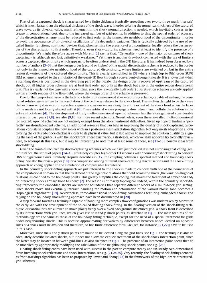
A step forward towards a technique capable of handling more complex flow configurations was undertaken by Moretti inthe early 70s with the development of the so-called floating shock-fitting. In the floating version of the shock-fitting tech-nique, discontinuities are allowed to move (float) freely over a fixed background structured grid. A shock front is describedby its intersections with grid lines, which gives rise to x and y shock points, as sketched in Fig. 1. The main features of themethodology are the same as those of the boundary fitting technique, except for the need of a special treatment for gridsnodes neighbouring shocks. This is because approximating derivatives by differences between nodes located on oppositesides of a shock must be avoided and therefore, ad hoc finite difference formulae (see, for instance, [21,22]) have to be usedin this case.

Moreover, since the x and y shock points are bound to be located along the grid lines, see Fig. 1, the technique is able toadequately describe isolated shocks, but it does not allow the explicit treatment of the shock-shock interaction point, sincethe latter may be located in between grid-lines, as also sketched in Fig. 1. The presence of an interaction point needs then tobe modelled by appropriately modifying the calculation of the neighbouring shock points, see e.g. [23].

Floating shock fitting codes have been used with success in the past to compute steady and un-steady two-dimensionalflows involving shock reflections and shock interactions, see e.g. [21,24,25]. Very recently, the floating shock-fitting (denotedas front-tracking) algorithm has been re-proposed by Rawat and Zhong [22] in the framework of the high-order, structured-grid schemes.

x

y

shock front gridpoints

shock nodes

shock interaction

Fig. 1. Shock points: �: x-shock; �: y-shock.

R. Paciorri, A. Bonfiglioli / Journal of Computational Physics 230 (2011) 3155–3177 3157

Nonetheless, floating shock fitting is an algorithmically complex technique primarily because of the need to interface aninherently unstructured collection of points used to represent the shock fronts with the underlying structured mesh, whichis described using the classical IJK data structure. A thorough account of these difficulties can be found in [22].

Building upon our experience in the areas of shock-fitting [26], on one hand, and unstructured grid techniques [27], onthe other hand, we have recently [28] developed a novel unstructured shock-fitting technique that makes use of the geomet-rical flexibility of unstructured meshes and combines features of both the boundary and floating shock-fitting techniques,which have always been used within the structured grid setting.

In this novel unstructured shock-fitting approach the shock front is discretised as a polygonal curve which is treated as aninternal boundary by the shock-capturing solver. The local shock speed and nodal values on the high pressure side of theshock are computed by enforcing the Rankine–Hugoniot (R–H) relations across the discontinuity. The shock is allowed tomove over and independently of a background triangular grid which is locally adapted at each time step to ensure that thenodes and the edges that make up the shock are part of a constrained Delaunay triangulation that covers the entire compu-tational domain. A shock-capturing, vertex centred, second-order-accurate solver which uses Fluctuation Splitting schemes[29] over triangular elements is used to approximate the governing PDEs in smooth regions of the flow-field. The couplingof the shock-fitting technique with a shock-capturing solver also enables an hybrid mode of operation in which some ofthe shocks are fitted, whereas all others are captured. This newly developed technique has been described and validated in[28] where it has been applied to the simulation of a moving planar shock wave and the bow shock that forms ahead of a bluntbody immersed in a hypersonic stream. In that same paper, the hybrid technique has been demonstrated by reference to aMach reflection in which the incident shock is captured whereas the reflected shock and the Mach stem are fitted.

In more recent work [30], two new features have been added to the aforementioned methodology: (i) not only shocks, butalso contact discontinuities are ‘‘fitted’’ and (ii) the triple point that arises in Mach reflections is analytically modelled usingvon Neumann’s three-shock-theory.

In this paper we generalise the treatment of shock interactions beyond that occurring at the triple point of a Mach reflec-tion (which has already been addressed in [30]) by including the interactions of shocks of the same and opposite families andthe regular reflection from a solid wall.

Section 2 reviews the basic ingredients of the shock-fitting algorithm for the treatment of isolated shocks and contact dis-continuities. Section 3 addresses the treatment of various types of shock interactions and also provides computational exam-ples. The capability of modeling explicitly the interaction point represents a new feature of the proposed unstructuredshock-fitting technique, which is not restricted to problems characterised by a simple topological structure. Section 4, whichreports the simulation of the Type IV interaction, demonstrates that the technique can also be applied to complex flows fea-turing multiple interactions.

The new features that have been added in this paper to the unstructured shock-fitting algorithm represents an importantstep towards the fine-tuning of a general-purpose shock-fitting technique. Indeed, in its current version, the proposed tech-nique still presents several important restrictions that limit its range of applicability. These restrictions, along with our plansfor future work, will be discussed in the conclusions.

2. Discontinuity fitting algorithm

The present discontinuity-fitting algorithm can be viewed as a local re-meshing strategy that generates a time dependentconstrained delaunay triangulation. This triangular mesh is constrained not only by the boundaries of the computational do-main, but also by the double-sided, polygonal curve that is used to describe the discontinuity.

When dealing with steady flows, as we do in the present paper, the steady solution is approached asymptotically follow-ing a pseudo transient. In the steady state, once the shock front has settled to its final position (corresponding to vanishingshock speed), the entire triangular mesh no longer changes.

phantom nodes

Cells crossed by shock

Phantomnodes

Cells enclosing

d l

Upstream

Shock

Downstream

Upstreamstate

Downstreamstate

Shockpoint

Internalboundary

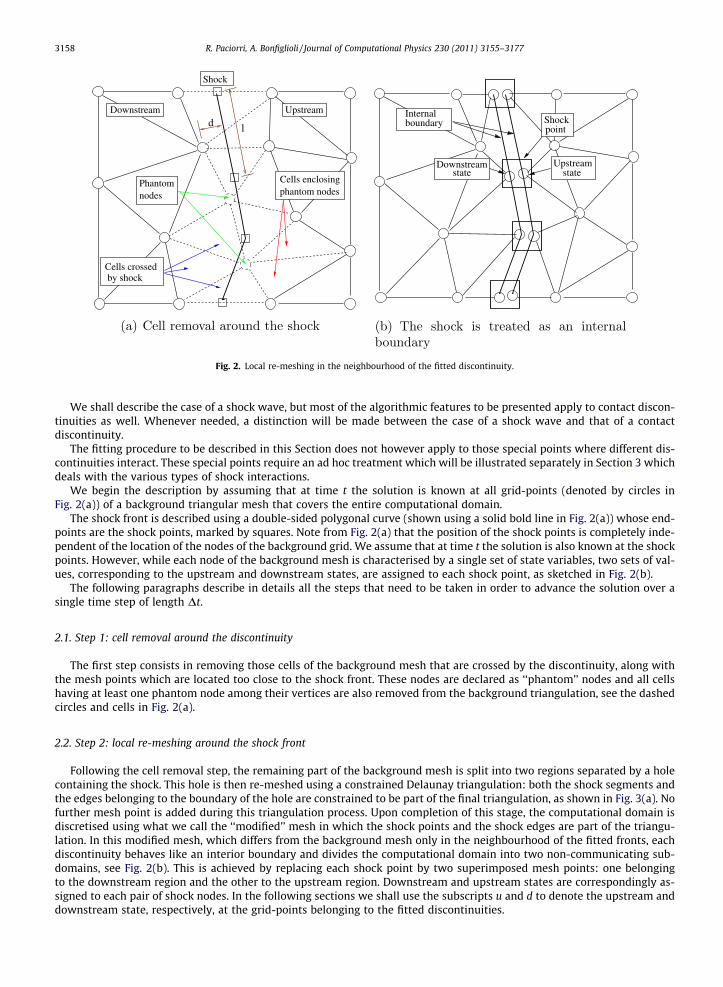
Fig. 2. Local re-meshing in the neighbourhood of the fitted discontinuity.


We shall describe the case of a shock wave, but most of the algorithmic features to be presented apply to contact discon-tinuities as well. Whenever needed, a distinction will be made between the case of a shock wave and that of a contactdiscontinuity.

The fitting procedure to be described in this Section does not however apply to those special points where different dis-continuities interact. These special points require an ad hoc treatment which will be illustrated separately in Section 3 whichdeals with the various types of shock interactions.

We begin the description by assuming that at time t the solution is known at all grid-points (denoted by circles inFig. 2(a)) of a background triangular mesh that covers the entire computational domain.

The shock front is described using a double-sided polygonal curve (shown using a solid bold line in Fig. 2(a)) whose end-points are the shock points, marked by squares. Note from Fig. 2(a) that the position of the shock points is completely inde-pendent of the location of the nodes of the background grid. We assume that at time t the solution is also known at the shockpoints. However, while each node of the background mesh is characterised by a single set of state variables, two sets of val-ues, corresponding to the upstream and downstream states, are assigned to each shock point, as sketched in Fig. 2(b).

The following paragraphs describe in details all the steps that need to be taken in order to advance the solution over asingle time step of length Dt.

2.1. Step 1: cell removal around the discontinuity

The first step consists in removing those cells of the background mesh that are crossed by the discontinuity, along withthe mesh points which are located too close to the shock front. These nodes are declared as ‘‘phantom’’ nodes and all cellshaving at least one phantom node among their vertices are also removed from the background triangulation, see the dashedcircles and cells in Fig. 2(a).

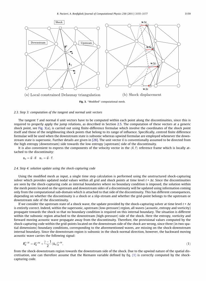
2.2. Step 2: local re-meshing around the shock front

Following the cell removal step, the remaining part of the background mesh is split into two regions separated by a holecontaining the shock. This hole is then re-meshed using a constrained Delaunay triangulation: both the shock segments andthe edges belonging to the boundary of the hole are constrained to be part of the final triangulation, as shown in Fig. 3(a). Nofurther mesh point is added during this triangulation process. Upon completion of this stage, the computational domain isdiscretised using what we call the ‘‘modified’’ mesh in which the shock points and the shock edges are part of the triangu-lation. In this modified mesh, which differs from the background mesh only in the neighbourhood of the fitted fronts, eachdiscontinuity behaves like an interior boundary and divides the computational domain into two non-communicating sub-domains, see Fig. 2(b). This is achieved by replacing each shock point by two superimposed mesh points: one belongingto the downstream region and the other to the upstream region. Downstream and upstream states are correspondingly as-signed to each pair of shock nodes. In the following sections we shall use the subscripts u and d to denote the upstream anddownstream state, respectively, at the grid-points belonging to the fitted discontinuities.

Shock

Downstream Upstreamτ

τ

n

n

wΔt

wΔt

wΔt

wΔt

Fig. 3. ‘‘Modified’’ computational mesh.


2.3. Step 3: computation of the tangent and normal unit vectors

The tangent ~s and normal ~n unit vectors have to be computed within each point along the discontinuities, since this isrequired to properly apply the jump relations, as described in Section 2.5. The computation of these vectors at a genericshock point, see Fig. 3(a), is carried out using finite-difference formulae which involve the coordinates of the shock pointitself and those of the neighbouring shock points that belong to its range of influence. Specifically, centred finite differenceformulae will be used when the downstream state is subsonic whereas upwind formulae are employed whenever the down-stream state is supersonic. Further details are given in [28]. The unit vector~n is conventionally assumed to be directed fromthe high entropy (downstream) side towards the low entropy (upstream) side of the discontinuity.

It is also convenient to express the components of the velocity vector in the ð~n;~sÞ reference frame which is locally at-tached to the discontinuity:

un ¼ ~u �~n us ¼~u �~s:

2.4. Step 4: solution update using the shock-capturing code

Using the modified mesh as input, a single time step calculation is performed using the unstructured shock-capturingsolver which provides updated nodal values within all grid and shock points at time level t + Dt. Since the discontinuitiesare seen by the shock-capturing code as internal boundaries where no boundary condition is imposed, the solution withinthe mesh points located on the upstream and downstream sides of a discontinuity will be updated using information comingonly from the computational sub-domain which is attached to that side of the discontinuity. This has different consequences,depending on whether the discontinuity is a shock or a slip-stream and whether the grid-point belongs to the upstream ordownstream side of the discontinuity.

If we consider the upstream state of a shock wave, the update provided by the shock-capturing solver at time level t + Dtis entirely correct. Indeed, within the supersonic, upstream (low-pressure) region, all waves (acoustic, entropy and vorticity)propagate towards the shock so that no boundary condition is required on this internal boundary. The situation is differentwithin the subsonic region attached to the downstream (high-pressure) side of the shock. Here the entropy, vorticity andforward moving acoustic wave propagate away from the discontinuity. Therefore, the provisional values computed by theshock-capturing code within the grid-points located on the downstream side of the shock are wrong, since three (in two spa-tial dimensions) boundary conditions, corresponding to the aforementioned waves, are missing on the shock-downstreaminternal boundary. Since the downstream region is subsonic in the shock-normal direction, however, the backward movingacoustic wave carries the following signal:

RtþDtd ¼ ~atþDt

d þ c� 12ð~unÞtþDt

d ; ð1Þ

from the shock-downstream region towards the downstream side of the shock. Due to the upwind nature of the spatial dis-cretisation, one can therefore assume that the Riemann variable defined by Eq. (1) is correctly computed by the shock-capturing code.


In Eq. (1) ~atþDtd and ~utþDt

d are the values of the sound speed and flow velocity of the downstream state of the shock nodescomputed by the shock-capturing solver. These flow variables have been marked with a ‘‘tilde’’ to underline the fact thatthese are the provisional (incorrect) values computed at time t + Dt by the shock-capturing code before enforcing the jumprelation across the discontinuity, as described in Section 2.5.

If a contact discontinuity is considered instead, both the upstream and downstream states are in general incorrect, exceptfor the following set of characteristic variables:

RtþDtd ¼ ~atþDt

d þ c� 12ð~unÞtþDt

d ; ð2aÞ

RtþDtu ¼ ~atþDt

u � c� 12ð~unÞtþDt

u ; ð2bÞ

StþDtd ¼

~ptþDtd

ð~qtþDtd Þc

; ð2cÞ

StþDtu ¼

~ptþDtu

ð~qtþDtu Þc

; ð2dÞ

VtþDtd ¼ ð~usÞtþDt

d ; ð2eÞVtþDt

u ¼ ð~usÞtþDtu : ð2fÞ

Indeed, these variables are associated with acoustic, entropy and vorticity waves that do not cross the boundary, and there-fore their correct evolution does not require any exchange of information across the contact discontinuity.

2.5. Step 5: enforcement of the jump relations

The missing pieces of information that are needed to correctly update the solution within the grid-points located on thediscontinuities are provided in the current step, which consists in enforcing the R–H relations between the upstream anddownstream states.

A different treatment is required for shocks and contact discontinuities. Let us first consider a shock point. For notationalconvenience, we introduce the flow velocity ~v relative to the discontinuity:

~v ¼~u� ~w; ð3Þ
~w being the velocity of the discontinuity relative to an inertial reference frame. As explained in Section 2.4, the shock up-stream state ð~uu; au;quÞ has been correctly updated at time level t + Dt by the shock-capturing solver. Concerning the down-stream state, however, only the Riemann variable RtþDt
d , given by Eq. (1), is assumed to be correctly computed by the shock-capturing solver.

The ‘‘correct’’ downstream state and the shock speed component wn ¼ ~w �~n normal to the discontinuity are then obtainedby solving a system of five non-linear algebraic equations.

qtþDtd ðvnÞtþDt

d ¼ qtþDtu ðvnÞtþDt

u ; ð4aÞ

ptþDtd þ qtþDt

d v2n

� �tþDt

d ¼ ptþDtu þ qtþDt

u v2n

� �tþDt

u ; ð4bÞðusÞtþDt

d ¼ ðusÞtþDtu ; ð4cÞ

HtþDtd ¼ HtþDt

u ; ð4dÞ

atþDtd þ c� 1

2ðunÞtþDt

d ¼ RtþDtd : ð4eÞ

The first four equations are the R–H jump relations, while the fifth equation enforces the ‘‘correct’’ information, given by Eq.(1), computed by the shock-capturing solver on the downstream side of the shock. In Eq. (4) H is the specific total enthalpy ofthe relative motion:

H ¼ cc� 1

pqþ v2

n þ v2t

2:

Observe that all variables in the left hand side of Eq. (4) are unknown, whereas all values on the right hand side (except theshock speed wn) are those ‘‘correctly’’ updated by the shock-capturing solver at time level t + Dt. The five unknown quantitiesare the downstream state: atþDt

d , qtþDtd , the two Cartesian components of~utþDt

u and the shock speed wtþDtn , since pressure can be

expressed as a function of sound speed and density. A Newton–Raphson algorithm is used to solve the system made up of Eq.(4) at each shock point.

Similar to a shock point, a grid-point belonging to a contact discontinuity is characterised by two states and by the veloc-ity of the discontinuity along the normal to the front ðwcd ¼ ~w �~nÞ. There are nine unknowns in total: the velocity compo-nents, density and pressure on both sides and the velocity of the discontinuity. All these variables can be updated at time


level t + Dt by solving an algebraic system of non-linear equations which comprises the jump relations for the contactdiscontinuity:

ptþDtu � ptþDt

d ¼ 0; ð5aÞðunÞtþDt

u �wtþDtcd ¼ 0; ð5bÞ

ðunÞtþDtd �wtþDt

cd ¼ 0; ð5cÞ

and the six ‘‘characteristic’’ equations:

atþDtd þ c� 1

2unð ÞtþDt

d ¼ RtþDtd ; ð6aÞ

atþDtu � c� 1

2unð ÞtþDt

u ¼ RtþDtu ; ð6bÞ

ptþDtd

ðqtþDtd Þc

¼ StþDtd ; ð6cÞ

ptþDtu

ðqtþDtu Þc

¼ StþDtu ; ð6dÞ

ðusÞtþDtd ¼ VtþDt

d ; ð6eÞðusÞtþDt

u ¼ VtþDtu : ð6fÞ

2.6. Step 6: computation of the interaction points

The grid-points belonging to a discontinuity where the interaction among different discontinuities occurs cannot be dealtwith using the approach described in Section 2.5, but require a specific modelling which depends upon the particular inter-action topology. The numerical treatment of these special points will therefore be illustrated for each different case in Sec-tion 3 where several flows featuring different kinds of interactions will be described.

2.7. Step 7: shock displacement

As shown in Fig. 3(b), the new position of the shock front at time t + Dt is obtained by displacing all discontinuity pointsusing the following first order integration formula:

PtþDt ¼ Pt þwtþDtnDt: ð7Þ

If Dt is kept small enough, the shock edges do not overcome any of the grid-points of the modified mesh, but only phantompoints that do not belong to the modified mesh used in present time step. In practice, Dt is chosen such that the shock pointmotion is confined within the hole dug in the background mesh by the cell removal step described in Section 2.1. By doing so,we avoid one of the steps we had considered in the earlier version of the algorithm reported in [28] which required the re-calculation of the flow state within those grid-points of the modified mesh that had been overcome by the movingdiscontinuity.

Phantomnode

Cell containgthe phantom node

Fig. 4. Phantom point interpolation.


Due to the displacement of the shock points, the modified mesh is deformed, as shown in Fig. 3(b). Since the shock motionhas been confined within the hole cut by the shock front within the background triangulation, the connectivity of the mod-ified mesh can be preserved even after the shock displacement, without risking the creation of degenerate cells. In Fig. 3(b)the edges of the modified mesh are shown by dashed and solid lines before and after shock displacement, respectively. Thisdeformed, modified mesh is only used to perform the interpolation of the phantom nodes which is described in Section 2.8.

2.8. Step 8: interpolation at the phantom nodes

In the previous steps all nodes of the modified mesh have been updated at time level t + Dt. Nevertheless the phantomnodes, which belong to the background mesh, but had been excluded from the modified mesh, have not been updated. Theneed to also update these nodes should be clear if we consider that at a later time the discontinuity might have moved suf-ficiently far away from its current position that some of the phantom nodes may be re-inserted into the modified mesh.

The update of the phantom nodes is performed by first locating each phantom node within the computational mesh (asearch operation which can be efficiently performed on a Delaunay mesh) and then using linear interpolation which is con-sistent with the linear elements adopted in the unstructured code (see Fig. 4).

This step is the last operation needed to advance the solution over a single time step. At this stage the modified mesh isdiscarded and the calculation of a new time step can begin.

3. Some simple interactions

Different types of interactions can be observed in real-life situations, such as those occurring when two shocks interact orwhen an incident shock is reflected off a wall. Four simple flows representing different types of interactions will be consid-ered in the next sections. In particular, the solutions obtained using the fully-fitted approach, in which all shocks, contactdiscontinuities and the interaction points are fitted, will be compared with those obtained using the shock-capturing ap-proach and/or the hybrid approach whereby some of the discontinuities are fitted whereas the remaining ones and the inter-action points are captured. As mentioned previously, each type of interaction requires an ad hoc treatment of the pointwhere the various discontinuities meet. For this reason a description of these ad hoc procedures used in the specific com-putation will be given in the next sections.

3.1. Interaction between two shocks of opposite families

The first type of shock-shock interaction to be considered is that originating from the collision of two shocks belonging todifferent families, see the sketch of Fig. 5(a). A uniform supersonic stream (zone 1) is traversed by two incident shocks (I1and I2) of opposite family and different strength which interact in the point QP (hereafter named quadruple point) giving riseto two outgoing reflected shocks (R1 and R2) and a contact discontinuity, or slip-stream (SS), located in between the

n12

τ12

α 13

4

15

2

δ 5

I2

3

wqp

QPM> 1

τ13n13

R1

I1

R2δ 3

α 35

δ 4

α 24

24τn24

δ 2

SS

Fig. 5. Interaction between two shocks of opposite families.

Table 1Interaction between two shocks of opposite families: analytical steady state solution.

1 2 3 4 5

M 3.0 2.255 1.994 1.461 1.432d 0.0 �15� 20� 4.796� 4.796�p/p1 1.0 2.822 3.771 8.353 8.353q/q1 1.0 2.034 2.420 4.263 4.211


reflected shocks. The incident and reflected shocks and the slip-stream bound five regions surrounding the quadruple point(denoted as zone 1, 2, 3, 4 and 5 in Fig. 5(a)), each characterised by uniform flow properties.

The exact steady state solution to this kind of flow can be computed from the known upstream flow state (zone 1) and theflow deflections (d2 and d3) caused by the two incident shocks. Table 1 reports, for each uniform-flow region, the analyticallycomputed Mach number (M), deflection angle (d) with respect to the horizontal, pressure (p/p1) and density (q/q1) ratios forM1 = 3, d2 = � 15� and d3 = 20�. This flow has been numerically computed using both the shock-capturing and the fully-fittedapproaches.

Before illustrating the results obtained by the numerical simulations, it is necessary to detail the numerical model used inthe fully-fitted computation of the quadruple point.

Let us start by assuming that at time t a modified mesh is available in which the quadruple point, the shocks and the con-tact discontinuity are part of the triangulation. In this modified mesh, which is shown in Fig. 5(b), the presence of the qua-druple point splits the computational domain into five non-communicating regions, each of these bounded by a pair ofdiscontinuities meeting at the quadruple point.

As mentioned in Section 2, all points located on a shock or slipstream are characterised by two sets of state variables, cor-responding to the upstream and downstream states. On the contrary, five different flow states need to be assigned to thequadruple point, each corresponding to the five regions shown in Fig. 5(a).

We begin the description of the quadruple point fitting procedure by noting that the computation of the normal and tan-gent unit vectors in the quadruple point according to the procedure described in Section 2.3 can be carried out without vio-lating the domain of dependence only for the incident shocks I1 and I2. On the contrary, the same procedure cannot beapplied to the reflected shocks R1 and R2, since the use of upwind finite difference formulae would involve shock points lo-cated beyond the endpoints of the R1 and R2 shocks. This observation highlights the fact that the slopes of the R1 and R2shocks at the quadruple point should be taken as unknowns. In practice, we use as unknown quantities the angle a formedby the shock and the flow direction in the uniform region 1, and denote as a24 and a35 the slopes of the R1 and R2 shocks atthe quadruple point. Observe that the normal and tangent unit vectors can be conveniently expressed in terms of the angle aas follows:

~n ¼ ðsina;� cos aÞT ~s ¼ ðcos a; sinaÞT :

When the shock-capturing code updates the solution at time level t + Dt within each of the five regions surrounding the qua-druple point, all five states associated with it will also be updated. However, only state 1 is ‘‘correctly’’ updated to time t + Dt,for the same reason explained in Section 2.4, whereas the other four states have not been correctly updated and, therefore,have to be re-computed by enforcing the jump relations at the quadruple point. In summary, the unknowns of the quadruplepoint problem are the states 2, 3, 4 and 5 at time t + Dt (16 unknowns), the slope of the R1 and R2 shocks (2 unknowns) andthe quadruple point velocity vector (2 unknown components) for a total number of 20 unknowns.

The calculation of these unknown quantities can be split into three sub-problems. Indeed, state 2 can be computed sep-arately using the shock point calculation described in Section 2.5 by taking the states 1 and 2 respectively equal to the up-stream and downstream ones and by setting ~n ¼~n12. The same procedure can be used to compute state 3. At this stage weare left with 12 unknowns. The shock speeds of the incident shocks I1 and I2 obtained by the solution of these two sub-problems allow to compute the quadruple point velocity vector ð~wQPÞ, since the position of the quadruple point only dependsupon the motion of the two incident shocks I1 and I2. Specifically, ~wQP can be obtained by a combination of the shock speed(wI1 and wI2) of I1 and I2 computed at the quadruple point:

~wQP ¼ awI1~n12 þ bwI2~n13;

where

a ¼ wI1ð~n12 �~n13Þ �wI2

wI2ð~n12 �~n13Þ2 �wI2;

b ¼ wI2ð~n12 �~n13Þ �wI1

wI1ð~n12 �~n13Þ2 �wI1:

The remaining ten unknowns are finally computed by solving a system of as many non-linear algebraic equations. Eight ofthese are the four R–H relations (4) written for both reflected shocks R1 and R2. In these eight jump relations the normal

0.8

0.85

0.1Supersonic inflow (state 2)

Supersonic inflow (state 3)

Su

per

son

ic in

flo

w (

stat

e 1)

Sp

erso

nic

ou

tflo

w

0.75

Fig. 6. Interaction of shocks of opposite families.


components of the shock speed wR1 and wR2 are a function of the quadruple point velocity vector ~wQP, since the motion of thereflected shocks is coupled to that of the quadruple point:

wR1 ¼ ~wQP �~n24 ¼ ~wQP � ðsin a24~ı� cos a24~|Þ; ð8aÞwR2 ¼ ~wQP �~n35 ¼ ~wQP � ðsin a35~ı� cos a35~|Þ: ð8bÞ

Note that Eq. (8) depends on the unknown slopes (a24 and a35) of the reflected shocks at the quadruple point. Finally, thesystem is closed by the jump relations for the slip-stream:

p4 � p5 ¼ 0; ð9aÞj~u4 �~u5j ¼ 0: ð9bÞ

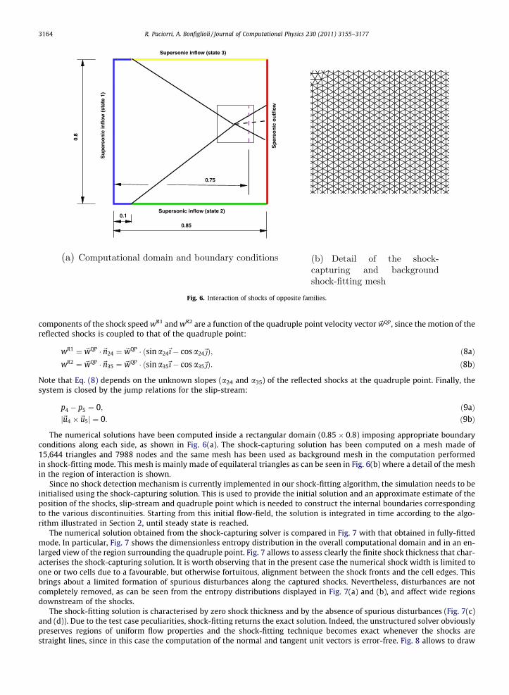
The numerical solutions have been computed inside a rectangular domain (0.85 � 0.8) imposing appropriate boundaryconditions along each side, as shown in Fig. 6(a). The shock-capturing solution has been computed on a mesh made of15,644 triangles and 7988 nodes and the same mesh has been used as background mesh in the computation performedin shock-fitting mode. This mesh is mainly made of equilateral triangles as can be seen in Fig. 6(b) where a detail of the meshin the region of interaction is shown.

Since no shock detection mechanism is currently implemented in our shock-fitting algorithm, the simulation needs to beinitialised using the shock-capturing solution. This is used to provide the initial solution and an approximate estimate of theposition of the shocks, slip-stream and quadruple point which is needed to construct the internal boundaries correspondingto the various discontinuities. Starting from this initial flow-field, the solution is integrated in time according to the algo-rithm illustrated in Section 2, until steady state is reached.

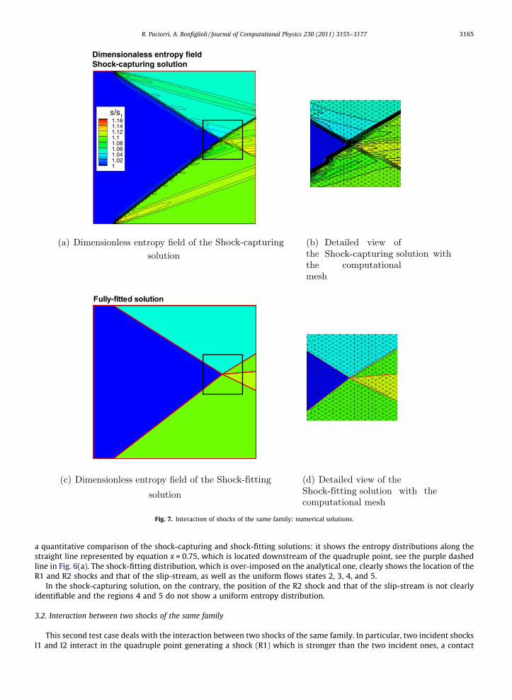
The numerical solution obtained from the shock-capturing solver is compared in Fig. 7 with that obtained in fully-fittedmode. In particular, Fig. 7 shows the dimensionless entropy distribution in the overall computational domain and in an en-larged view of the region surrounding the quadruple point. Fig. 7 allows to assess clearly the finite shock thickness that char-acterises the shock-capturing solution. It is worth observing that in the present case the numerical shock width is limited toone or two cells due to a favourable, but otherwise fortuitous, alignment between the shock fronts and the cell edges. Thisbrings about a limited formation of spurious disturbances along the captured shocks. Nevertheless, disturbances are notcompletely removed, as can be seen from the entropy distributions displayed in Fig. 7(a) and (b), and affect wide regionsdownstream of the shocks.

The shock-fitting solution is characterised by zero shock thickness and by the absence of spurious disturbances (Fig. 7(c)and (d)). Due to the test case peculiarities, shock-fitting returns the exact solution. Indeed, the unstructured solver obviouslypreserves regions of uniform flow properties and the shock-fitting technique becomes exact whenever the shocks arestraight lines, since in this case the computation of the normal and tangent unit vectors is error-free. Fig. 8 allows to draw

Fully-fitted solution

Dimensionaless entropy fieldShock-capturing solution

s/s11.161.141.121.11.081.061.041.021

Fig. 7. Interaction of shocks of the same family: numerical solutions.


a quantitative comparison of the shock-capturing and shock-fitting solutions: it shows the entropy distributions along thestraight line represented by equation x = 0.75, which is located downstream of the quadruple point, see the purple dashedline in Fig. 6(a). The shock-fitting distribution, which is over-imposed on the analytical one, clearly shows the location of theR1 and R2 shocks and that of the slip-stream, as well as the uniform flows states 2, 3, 4, and 5.

In the shock-capturing solution, on the contrary, the position of the R2 shock and that of the slip-stream is not clearlyidentifiable and the regions 4 and 5 do not show a uniform entropy distribution.

3.2. Interaction between two shocks of the same family

This second test case deals with the interaction between two shocks of the same family. In particular, two incident shocksI1 and I2 interact in the quadruple point generating a shock (R1) which is stronger than the two incident ones, a contact

s/s1

Y

1 1.05 1.10.35

0.4

0.45

0.5

0.55shock−capturing

shock−fitting

SS

R2

R1

2

3

4

5

Dimensionless entropy distribution at x=0.75

Fig. 8. Interaction of shocks of opposite families: comparison between the entropy distribution at x = 0.75.

Enlarged boxnodes: 7988triangles: 15644

0.8

0.85

0.137

Supersonic inflow(state 1)

Supersonic inflow (state 2)Su

pers

onic

inflo

w(s

tate

2)

Sper

soni

cou

tflow

0.237

Supersonic inflow(state 3)α 13

4

5

δ 5

1

n12

τ12

2

3

wqp

M> 1

R1

R2δ 3

α 35

δ 4

α24

δ 1

I1 I2

SSτ 24

24n

QP

τ13n13

Fig. 9. Interaction between two shocks of the same family: computational domain and boundary conditions.


discontinuity (SS) and a reflected shock wave (R2) of nearly negligible strength. The R2 wave might be a weak expansion orcompression, depending on the free-stream flow Mach number and the flow deflections through the incident shocks. From atopological view point, this case is very similar to the previous one. Indeed, if we adopt the nomenclature of the zones andthe shocks reported in Fig. 9(a), the only topological difference between the present and the previous interaction is the ori-entation of the unit vector normal to the incident shock I1: in the present case the vector points from zone 1 to zone 2,whereas in the previous case the vector orientation was opposite. Similar to the interaction of shocks belonging to differentfamilies, the steady state solution can be analytically computed from the known upstream state 2 and the flow deflections(d1,d3) induced by the two incident shocks. Table 2 reports the flow states within each region of uniform flow computedassuming M2 = 2.0, d1 = 10� and d3 = 20�.

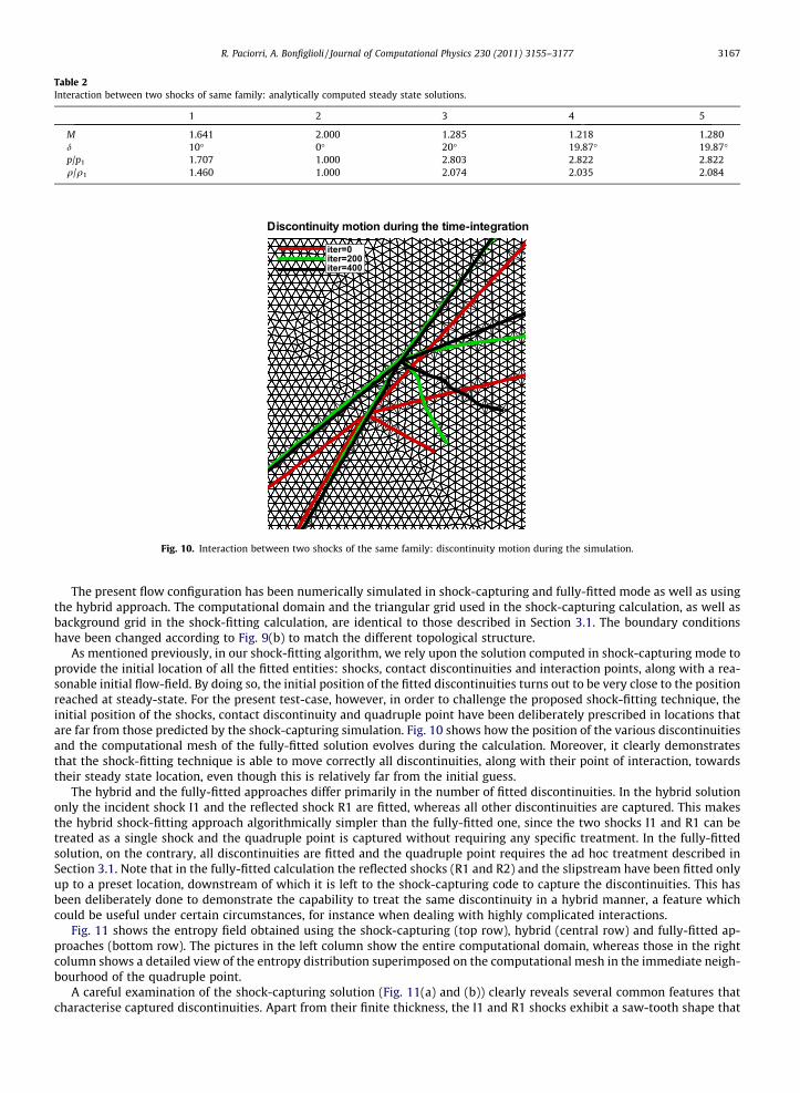
Table 2Interaction between two shocks of same family: analytically computed steady state solutions.

1 2 3 4 5

M 1.641 2.000 1.285 1.218 1.280d 10� 0� 20� 19.87� 19.87�p/p1 1.707 1.000 2.803 2.822 2.822q/q1 1.460 1.000 2.074 2.035 2.084

iter=0iter=200iter=400

Discontinuity motion during the time-integration

Fig. 10. Interaction between two shocks of the same family: discontinuity motion during the simulation.


The present flow configuration has been numerically simulated in shock-capturing and fully-fitted mode as well as usingthe hybrid approach. The computational domain and the triangular grid used in the shock-capturing calculation, as well asbackground grid in the shock-fitting calculation, are identical to those described in Section 3.1. The boundary conditionshave been changed according to Fig. 9(b) to match the different topological structure.

As mentioned previously, in our shock-fitting algorithm, we rely upon the solution computed in shock-capturing mode toprovide the initial location of all the fitted entities: shocks, contact discontinuities and interaction points, along with a rea-sonable initial flow-field. By doing so, the initial position of the fitted discontinuities turns out to be very close to the positionreached at steady-state. For the present test-case, however, in order to challenge the proposed shock-fitting technique, theinitial position of the shocks, contact discontinuity and quadruple point have been deliberately prescribed in locations thatare far from those predicted by the shock-capturing simulation. Fig. 10 shows how the position of the various discontinuitiesand the computational mesh of the fully-fitted solution evolves during the calculation. Moreover, it clearly demonstratesthat the shock-fitting technique is able to move correctly all discontinuities, along with their point of interaction, towardstheir steady state location, even though this is relatively far from the initial guess.

The hybrid and the fully-fitted approaches differ primarily in the number of fitted discontinuities. In the hybrid solutiononly the incident shock I1 and the reflected shock R1 are fitted, whereas all other discontinuities are captured. This makesthe hybrid shock-fitting approach algorithmically simpler than the fully-fitted one, since the two shocks I1 and R1 can betreated as a single shock and the quadruple point is captured without requiring any specific treatment. In the fully-fittedsolution, on the contrary, all discontinuities are fitted and the quadruple point requires the ad hoc treatment described inSection 3.1. Note that in the fully-fitted calculation the reflected shocks (R1 and R2) and the slipstream have been fitted onlyup to a preset location, downstream of which it is left to the shock-capturing code to capture the discontinuities. This hasbeen deliberately done to demonstrate the capability to treat the same discontinuity in a hybrid manner, a feature whichcould be useful under certain circumstances, for instance when dealing with highly complicated interactions.

Fig. 11 shows the entropy field obtained using the shock-capturing (top row), hybrid (central row) and fully-fitted ap-proaches (bottom row). The pictures in the left column show the entire computational domain, whereas those in the rightcolumn shows a detailed view of the entropy distribution superimposed on the computational mesh in the immediate neigh-bourhood of the quadruple point.

A careful examination of the shock-capturing solution (Fig. 11(a) and (b)) clearly reveals several common features thatcharacterise captured discontinuities. Apart from their finite thickness, the I1 and R1 shocks exhibit a saw-tooth shape that

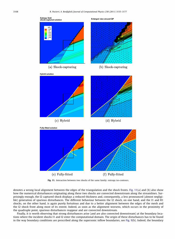
Fig. 11. Interaction between two shocks of the same family: entropy iso-contours.


denotes a wrong local alignment between the edges of the triangulation and the shock fronts. Fig. 11(a) and (b) also showhow the numerical disturbances originating along these two shocks are convected downstream along the streamlines. Sur-prisingly enough, the I2 captured shock displays a reduced thickness and, consequently, a less pronounced (almost negligi-ble) generation of spurious disturbances. The different behaviour between the I2 shock, on one hand, and the I1 and R1shocks, on the other hand, is again purely fortuitous and due to a better alignment between the edges of the mesh andthe I2 shock front along most of its extent. Indeed, as soon as the alignment worsens, which occurs in the proximity ofthe quadruple point, spurious disturbances reappear and are convected downstream.

Finally, it is worth observing that strong disturbances arise (and are also convected downstream) at the boundary loca-tions where the incident shocks I1 and I2 enter the computational domain. The origin of these disturbances has to be foundin the way boundary conditions are prescribed along the supersonic inflow boundaries, see Fig. 9(b). Indeed, the boundary

Table 3Regular reflection: steady state solution.

1 2 4

M 2.0 1.641 1.287d 0� �10� 0�p/p1 1.0 1.706 2.797q/q1 1.0 1.458 2.069

412

R1

I1

IP

M> 1

IPw

δ2

Fig. 12. Sketch of a regular reflection.

W = 2

H=

1

Wall

Supe

rson

ic in

flow

(sta

te 1

)

Supersonic inflow (state 2)Su

pers

onic

out

flow

IP

A detailed view of the mesh around IP

Fig. 13. Regular reflection off a wall: computational domain and background mesh.


condition does not take into account the finite thickness of the captured shocks so that a significant discrepancy arisesbetween the profile imposed along the inlet boundaries and that computed by the shock-capturing solver in the proximityof the boundaries. These problems are partly overcome by the solution obtained using the hybrid operational mode.Fig. 11(c) and (d) show that the production of numerical disturbances is completely suppressed along the entire extent ofthe I1 shock and the fitted part of R1 shock, whereas spurious disturbances re-appear along the captured portion of theR1 shock. Even the I2 shock, which is captured in the hybrid solution, features reduced disturbances with respect to theshock-capturing calculation (compare Fig. 11(a) with Fig. 11(c)) which is due to the fact that in the shock-capturing calcu-lation some of the disturbances arising along the I2 shock are caused by similar disturbances generated along the I1 shock,which are absent in the hybrid solution since in this latter case the I1 shock is fitted. Even if the solution in the proximity ofthe incident shock I2 and the slip-stream displays the same features of the shock-capturing solution (I2 and SS are capturedin the hybrid solution) the overall quality of the hybrid solution looks better than that obtained by capturing all discontinu-ities, i.e. the shock-capturing calculation.

A remarkable improvement in solution quality is achieved with the fully-fitted solution (Fig. 11(e) and (f)). Specifically, inregions where all discontinuities are fitted, the solution does not display any spurious disturbance. Moreover, since theregions bounded by the discontinuities are characterised by uniform flow states, the result is grid-independent, for the samereasons given in Section 3.1. As mentioned previously, the reflected shock and the slipstream have not been fitted all the waydown to the outflow boundary: as soon as the discontinuity is no longer fitted a captured discontinuity builds up andreplaces the fitted one. This can be clearly seen in Fig. 11(e). Transition from a region where the discontinuity is fitted toone where the discontinuity is captured occurs without any particular problems.


3.3. Shock–wall interaction: regular reflection

When a weak oblique shock wave impinges on a straight wall, two flow configurations can occur: the regular or the Machreflection. A regular reflection takes place whenever the flow deflection imposed by the straight wall is lower than the max-imum deflection that the supersonic stream behind the impinging shock can sustain. If the deflection is larger than this lim-iting value, a Mach reflection occurs. In the present section a simple flow reproducing the former configuration is analysed,whereas the latter configuration will be studied in the next section.

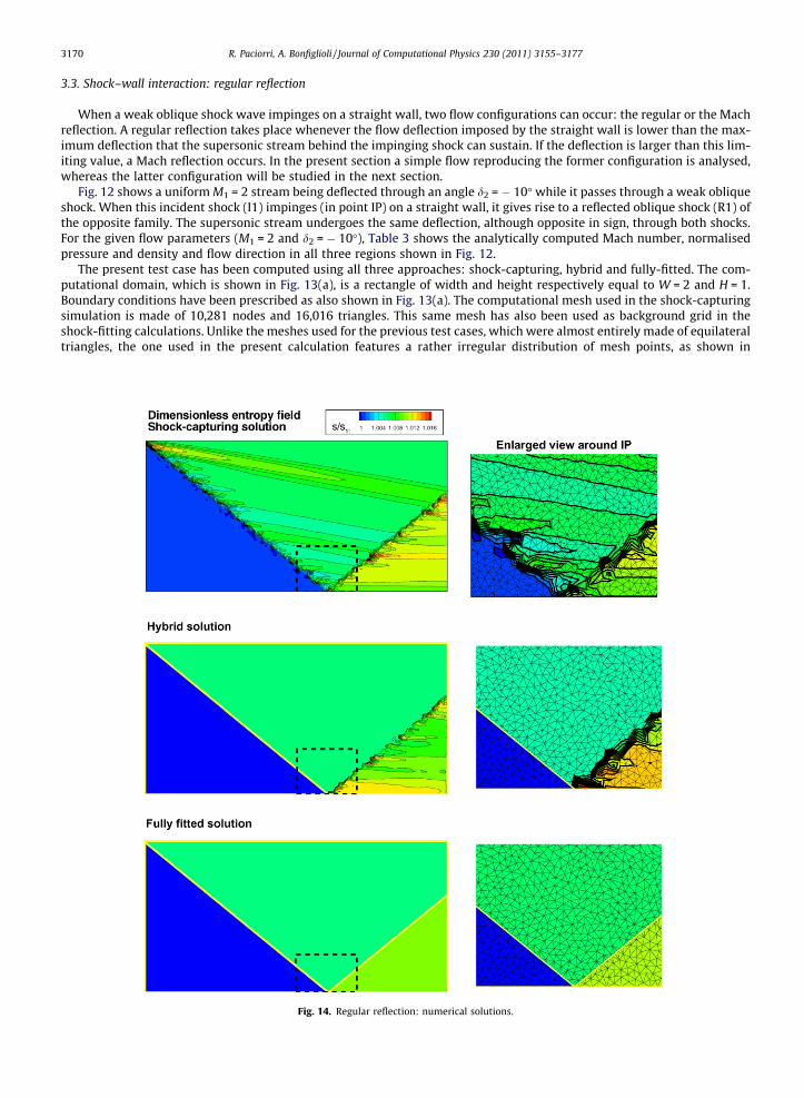
Fig. 12 shows a uniform M1 = 2 stream being deflected through an angle d2 = � 10� while it passes through a weak obliqueshock. When this incident shock (I1) impinges (in point IP) on a straight wall, it gives rise to a reflected oblique shock (R1) ofthe opposite family. The supersonic stream undergoes the same deflection, although opposite in sign, through both shocks.For the given flow parameters (M1 = 2 and d2 = � 10�), Table 3 shows the analytically computed Mach number, normalisedpressure and density and flow direction in all three regions shown in Fig. 12.

The present test case has been computed using all three approaches: shock-capturing, hybrid and fully-fitted. The com-putational domain, which is shown in Fig. 13(a), is a rectangle of width and height respectively equal to W = 2 and H = 1.Boundary conditions have been prescribed as also shown in Fig. 13(a). The computational mesh used in the shock-capturingsimulation is made of 10,281 nodes and 16,016 triangles. This same mesh has also been used as background grid in theshock-fitting calculations. Unlike the meshes used for the previous test cases, which were almost entirely made of equilateraltriangles, the one used in the present calculation features a rather irregular distribution of mesh points, as shown in

Fig. 14. Regular reflection: numerical solutions.

4

2

1

3TPw

MS

SSTP

R1

I1

M > 11

Fig. 15. Sketch of a Mach reflection.


Fig. 13(b), where a detailed view of the area bordered by the dashed line in Fig. 13(a) which surrounds the impingementpoint IP is displayed.

Before discussing the numerical results it is worth describing the procedure used to model the impingement point IP inthe fully-fitted simulation.

It is easy to show that regular reflections can be viewed as a subset of the more general case dealing with the interactionof shocks of different families, which has already been described in Section 3.1. Referring to Fig. 5(a), we note that wheneverthe two incident shocks I1 and I2 have the same strength, the flow becomes symmetric with respect to the horizontal linepassing through the quadruple point QP. The flow in region 4 is aligned with the horizontal direction and the quadruple pointQP can only move along the line of symmetry, which behaves like an inviscid wall. Moreover, the slip-stream vanishes, sinceit separates two regions (4 and 5) that have identical flow features. Using this artifice, we can deal with regular reflections bymeans of the more general approach that has already been described in Section 3.1. In particular, we are able to determinethe speed of the impingement point (wIP in Fig. 13(a)) and the flow states in regions 2 and 4.

Fig. 14 shows the computed entropy field for all three sets of calculations. Subfigures, from top to bottom, refer to theshock-capturing, hybrid and fully-fitted simulations. Within each sub-figure, the frame on the left shows the entropy fieldin the overall computational domain, whereas that on the right shows an enlargement of the region around the impingementpoint, over-plot on the mesh.

The captured shocks (both in the shock-capturing and hybrid calculations) are characterised by the presence of spuriousdisturbances that appear to be even stronger than those observed in the previous test-cases. The reason is related to the dif-ferent mesh patterns used in the present and previous test-cases.

When using highly irregular triangulation patterns, such as the one shown in Fig. 13(b), there is little hope that the shockfront may ever happen to be aligned with the edges of the triangulation. This is a more realistic situation than that observedin the previous two test-cases (see Sections 3.1 and 3.2) where the fortuitous alignment between the cell edges and theshock fronts limited the amount of spurious disturbances. Indeed, whenever the shocks are curved, it is very unlikely tobe able to construct an a priori triangulation that is able to align its edges with the shock front. Although it is true that aposteriori, anisotropic mesh adaptation can considerably improve the quality of a captured discontinuity, it is also true thatit will very likely lead to an increase in the number of grid-points and triangles, since mesh refinement in the shock-normaldirection generally outweighs mesh coarsening in the smooth regions of the flow. We can thus affirm that the present test-case allows better than the previous two to draw a fair comparison between shock-capturing and shock-fitting for a givengrid size, equal to both approaches.

Note that if we were dealing with shock reflection off a curved wall, some modifications to the algorithm we have justpresented would be needed, but this is left for future work.

3.4. Shock–wall interaction: Mach reflection

A Mach reflection occurs whenever the flow deflection through the incident shock is larger than the maximum deflectionangle that the flow downstream of the incident shock can sustain. Using the same free-stream conditions of the previouscase and increasing the deflection angle up to 14�, a Mach reflection occurs. As sketched in Fig. 15, in addition to the incidentshock (I1) and the reflected shock (R1), a strong shock, namely the Mach stem (MS), and a slip-stream (SS) appear in theflow-field and all these discontinuities meet at the triple point (TP). Although the flow regions behind the reflected shockand the Mach stem are characterised by non-uniform states and thus are not amenable to an analytical treatment, the solu-tion at the triple point can be analytically determined using von Neumann’s three-shock-theory. For the given free-streamconditions (M1 = 2 and d2 = � 14�) the analytically computed solution is reported in Table 4.

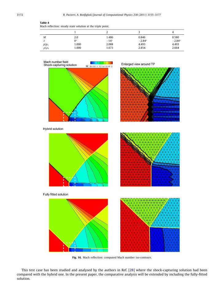
Table 4Mach reflection: steady state solution at the triple point.

1 2 3 4

M 2.0 1.486 0.846 0.580d 0� �14� �2.84� �2.84�p/p1 1.000 2.088 4.493 4.493q/q1 1.000 1.673 2.854 2.664

Fig. 16. Mach reflection: computed Mach number iso-contours.


This test case has been studied and analysed by the authors in Ref. [28] where the shock-capturing solution had beencompared with the hybrid one. In the present paper, the comparative analysis will be extended by including the fully-fittedsolution.


The computational domain, the boundary conditions and the background mesh for the fully-fitted simulation are thesame used in Ref. [28] for the shock-capturing and hybrid simulations.

The treatment of the triple point is similar to that of the quadruple point described in Section 3.1, but not identical, sincethe flow topology described in Fig. 15 cannot be recast into that shown in Fig. 5(a).

Since the triple point treatment has been extensively described in a recent paper [30], it will not be repeated here, butonly a set of relevant computational results will be presented.

The solutions obtained using the three different approaches are compared in Fig. 16: the shock-capturing, hybrid andfully-fitted solutions are displayed from top to bottom.

The top frame of Fig. 16 shows clearly that when a strong shock, such as the Mach stem, is captured using a triangulationwhose edges are poorly aligned with the shock front, the solution quality is remarkably deteriorated. Note the meandering

M∞

R

x

y

σ

shockSS

P

expansion

Fig. 17. Test case definition and flow sketch.

Fig. 18. Type IV interaction; shock-capturing approach: all shocks and contact discontinuities are computed by the shock-capturing solver.


shape of the captured Mach stem and how the spurious disturbances generated along its front are propagated downstream,polluting the entire subsonic region which is downstream of the Mach stem.

In the hybrid solution, which is shown in the central frame of Fig. 16, the reflected shock and the Mach stem have beenfitted, whereas the incident shock and the slip-stream have been captured. In general, the point where a fitted discontinuityinteracts with a captured one (the triple point in the present case) cannot any longer be dealt with using the fittingapproaches described in these sections, but it has to be captured by the shock-capturing solver. Although this simplifiesthe calculation, which does not any longer require a specific treatment of the point of interaction, the resolution is inferiorto that achievable by a fully-fitted technique. The hybrid solution shown in Fig. 16 does indeed show a smoother Mach dis-tribution in the region downstream of the Mach stem, but not as clean as the one computed using the fully-fitted approach,which is displayed in the bottom frame of Fig. 16.

4. A complex shock–shock interaction

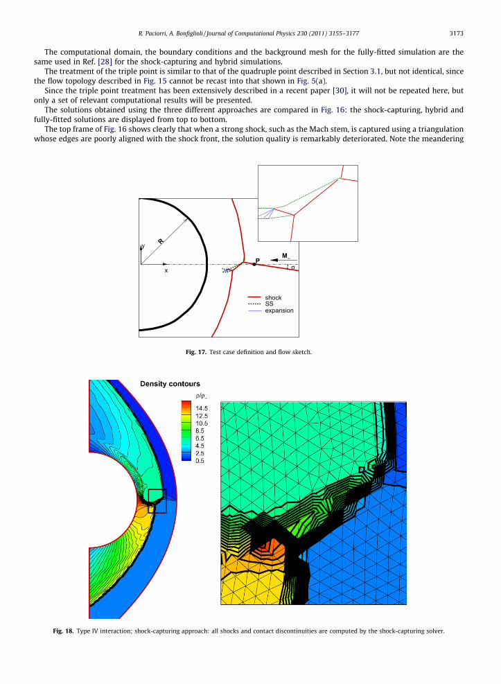
To assess the potential and the performances of this shock-fitting technique, a flow characterised by multiple interactionshas been computed. The selected flow is a type IV shock–shock interaction [31]. Fig. 17 shows a sketch of the flow structure.This type of interaction arises when a weak oblique shock impinges on the bow shock produced by a supersonic streamwhich impinges on the fore-body of a circular cylinder. The free-stream Mach number is M1 = 10 and the oblique shock, hav-ing slope r = 10�, crosses the x axis at a point P located at xP/R = 1.6666, R being the cylinder radius.

A first triple point forms at the point where the oblique shock impinges on the bow shock. A reflected shock and a contactdiscontinuity arise in this triple point and move downstream. The contact discontinuity separates the supersonic streamwhich has crossed the reflected oblique shock from the subsonic flow downstream of the bow shock. The reflected shockcoming from the first triple point re-joins the bow shock in a second triple point where a new reflected shock and a contactdiscontinuity arise. The two contact discontinuities bound a supersonic jet which is directed towards the body surface,whereas the second reflected shock triggers a series of wave reflections inside the supersonic jet bounded by the two contactdiscontinuities.

This flow has been computed using all the available computational modes: shock-capturing, hybrid and fully-fitted. Allsolutions have been computed starting from the same background mesh made of 10,855 nodes and 21,127 triangles. Sincethe shock-fitting procedure performs local modifications of the background mesh only in the neighbourhood of the fitteddiscontinuities, the number of grid-points and triangles is roughly the same in all three simulations.

Fig. 18 displays the computed density iso-contours obtained using the shock-capturing approach. In the right frame anenlargement of the region where the interaction takes place allows a better assessment of some details of the numericalsolution in relation to the computational mesh.

Fig. 19. Type IV interaction; hybrid approach: the bow shocks and the oblique shock connecting the triple points are fitted; the remaining shocks andcontact discontinuities are computed by the shock-capturing solver.

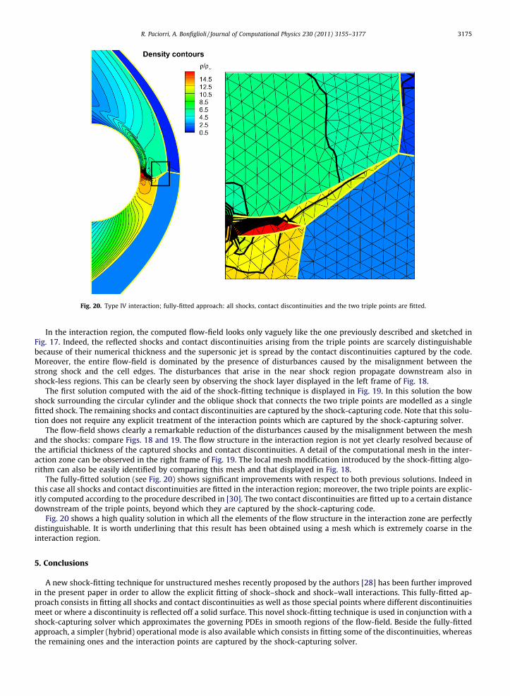
Fig. 20. Type IV interaction; fully-fitted approach: all shocks, contact discontinuities and the two triple points are fitted.


In the interaction region, the computed flow-field looks only vaguely like the one previously described and sketched inFig. 17. Indeed, the reflected shocks and contact discontinuities arising from the triple points are scarcely distinguishablebecause of their numerical thickness and the supersonic jet is spread by the contact discontinuities captured by the code.Moreover, the entire flow-field is dominated by the presence of disturbances caused by the misalignment between thestrong shock and the cell edges. The disturbances that arise in the near shock region propagate downstream also inshock-less regions. This can be clearly seen by observing the shock layer displayed in the left frame of Fig. 18.

The first solution computed with the aid of the shock-fitting technique is displayed in Fig. 19. In this solution the bowshock surrounding the circular cylinder and the oblique shock that connects the two triple points are modelled as a singlefitted shock. The remaining shocks and contact discontinuities are captured by the shock-capturing code. Note that this solu-tion does not require any explicit treatment of the interaction points which are captured by the shock-capturing solver.

The flow-field shows clearly a remarkable reduction of the disturbances caused by the misalignment between the meshand the shocks: compare Figs. 18 and 19. The flow structure in the interaction region is not yet clearly resolved because ofthe artificial thickness of the captured shocks and contact discontinuities. A detail of the computational mesh in the inter-action zone can be observed in the right frame of Fig. 19. The local mesh modification introduced by the shock-fitting algo-rithm can also be easily identified by comparing this mesh and that displayed in Fig. 18.

The fully-fitted solution (see Fig. 20) shows significant improvements with respect to both previous solutions. Indeed inthis case all shocks and contact discontinuities are fitted in the interaction region; moreover, the two triple points are explic-itly computed according to the procedure described in [30]. The two contact discontinuities are fitted up to a certain distancedownstream of the triple points, beyond which they are captured by the shock-capturing code.

Fig. 20 shows a high quality solution in which all the elements of the flow structure in the interaction zone are perfectlydistinguishable. It is worth underlining that this result has been obtained using a mesh which is extremely coarse in theinteraction region.

5. Conclusions

A new shock-fitting technique for unstructured meshes recently proposed by the authors [28] has been further improvedin the present paper in order to allow the explicit fitting of shock–shock and shock–wall interactions. This fully-fitted ap-proach consists in fitting all shocks and contact discontinuities as well as those special points where different discontinuitiesmeet or where a discontinuity is reflected off a solid surface. This novel shock-fitting technique is used in conjunction with ashock-capturing solver which approximates the governing PDEs in smooth regions of the flow-field. Beside the fully-fittedapproach, a simpler (hybrid) operational mode is also available which consists in fitting some of the discontinuities, whereasthe remaining ones and the interaction points are captured by the shock-capturing solver.


Both the fully-fitted and hybrid techniques have been successfully applied to different kinds of shock–shock interactionsand shock–wall reflections, including a complex type IV shock–shock interaction.

The results obtained using the fully-fitted mode are characterised by an extremely high quality as compared to the shock-capturing and hybrid solutions computed on meshes of comparable grid spacing.

The analysis of the results obtained using the unstructured shock-fitting technique and of its algorithmic features allowsus to make same general comments and assessments about the relative merits of this newly developed unstructured shock-fitting technique with respect to the classical shock-fitting techniques based on the structured meshes and the unstructuredshock-capturing techniques presently used in CFD.

The proposed shock-fitting technique appears to combine the implementation simplicity of the ‘‘boundary’’ shock-fittingtechnique with the capability of treating complex flows with shocks of the ‘‘floating’’ shock-fitting technique. Nevertheless, itdoes not seem to suffer the strong topological limitations that plagued the boundary shock-fitting technique when imple-mented in the structured grid context. Moreover, the integration of the present shock-fitting technique with a pre-existinggas-dynamic solver is algorithmically less complicated than the integration of the floating shock-fitting technique within astructured-grid solver. Finally, when compared to the traditional floating shock-fitting technique for structured grids, thepresent unstructured implementation allows the explicit treatment of the interaction points which was not entirely possiblewith the floating shock-fitting technique for structured meshes.

To summarise, the implementation of the shock-fitting technique in the unstructured grid framework appears to be sim-pler and more general than the traditional shock-fitting implementations for structured grids.

The shock-fitting technique is potentially able to solve many of the drawbacks that currently plague the shock-capturingsolutions, such as, for instance, the presence of spurious disturbances due to the misalignment between the shock front andthe mesh edges, the reduction of the order of accuracy in the smooth regions downstream of the shock and the carbunclephenomenon.

Nevertheless, it is clear that at present there are several serious impediments that make the replacement of the shock-capturing technique with the shock-fitting technique un-feasible for general-purpose applications. More precisely, the pro-posed shock-fitting technique is currently unable to automatically detect the formation of shocks and contact discontinuitiesand to figure out how these may be mutually connected at the interaction points. This latter information is of topologicalnature and may change during an un-steady calculation. To circumvent the aforementioned limitations, the proposed tech-nique currently relies on a preliminary shock-capturing calculation to provide an initial location of the discontinuities andtheir interaction points and it also requires an a priori knowledge of the flow topology that is not allowed to change duringthe simulation. These limitations considerably restrict the applicability of the present technique to practical problems sincethe user’s intervention is required to set-up the flow topology and to initialize the flowfield. Moreover, they represent a par-ticularly serious obstacle to the simulation of unsteady flows. It may be possible, even if not straightforward, to enhance thecurrent shock-fitting algorithm by making it capable to automatically detect the discontinuities, the overall flow topologyand the changes it might incur during an un-steady simulation. Up to now, these developments have been deliberatelyset aside by the authors who preferred to focus their efforts towards the numerical modelling of the interactions, whichhas been discussed in the present article, and the extension of the unstructured shock-fitting methodology to the three-dimensional space, which is documented in [32]. It is however clear that the aforementioned issues can no longer be ignoredand, therefore, the authors’ efforts will be concentrated in this direction in the near future. In this respect, it is worth to pointout that shock detection mechanisms have already been proposed in the shock-fitting literature, see e.g. [1] for a compre-hensive review. On the other hand, the capability to automatically identify changes in the flow topology, such as those occur-ring in un-steady shock interactions, is a quite formidable task from an algorithmic viewpoint. However, as observed byMoretti [19], this has more to do with topology than fluid mechanics and some expertise from other areas of computer sci-ence (artificial intelligence, for instance) might help in making shock-fitting a more versatile technique.

Despite the development of the present technique is still in its early phase and some important aspects are still beingcompletely ignored by the algorithm, we believe that unstructured shock-fitting techniques, if further developed, could be-come a valuable alternative to the universally used shock-capturing paradigm at least in those cases where high quality solu-tions are required (in aeroacoustic computations, for instance) and/or when capturing the shocks creates severe drawbacks(in hypersonic simulations, for instance) that oblige to use expensive remedies, such as mesh-adaption and mesh-refinement.

Appendix A. Supplementary material

Supplementary data associated with this article can be found, in the online version, at doi:10.1016/j.jcp.2011.01.018.

References

[1] M. Salas, A Shock-Fitting Primer, CRC Applied Mathematics & Nonlinear Science, first ed., Chapman & Hall, 2009.[2] G. Moretti, Computation of flows with shocks., Annual Review of Fluid Mechanics 19 (1987) 313–317.[3] D. Bonhaus, A higher order accurate finite element method for viscous compressible flows, Ph.D. Thesis, Virginia Polytechnic Institute and State

University, 1998.[4] M.H. Carpenter, J.H. Casper, Accuracy of shock capturing in two spatial dimensions, AIAA Journal 37 (9) (1999) 1072–1079.[5] C.J. Roy, Grid convergence error analysis for mixed-order numerical schemes, AIAA Journal 41 (4) (2003) 595–604.



[6] T.K. Lee, X. Zhong, Spurious numerical oscillations in simulation of supersonic flows using shock-capturing schemes, AIAA Journal 37 (3) (1999) 313–319.

[7] C. Rumsey, B. van Leer, A grid-independent approximate Riemann solver with applications to the Euler and Navier–Stokes equations, in: 29th AIAA,Aerospace Sciences Meeting, Reno, NV, 1991, p. 1991.

[8] A. Dadone, B. Grossman, A multi-dimensional upwind scheme for the Euler equations, in: M. Napolitano, F. Sabetta (Eds.), Thirteenth InternationalConference on Numerical Methods in Fluid Dynamics, Lecture Notes in Physics, vol. 414, Springer, Berlin Heidelberg, 1993, pp. 95–99. 10.1007/3-540-56394-6_195.

[9] P.A. Gnoffo, Multi-dimensional, inviscid flux reconstruction for simulation of hypersonic heating on tetrahedral grids, in: 47th AIAA Aerospace SciencesMeeting, Orlando, Florida, 2009 (Paper 2009-599).

[10] P.A. Gnoffo, Update to multi-dimensional flux reconstruction for hypersonic simulation on tetrahedral grids, in: 48th AIAA Aerospace SciencesMeeting, Orlando, Florida, 2010 (Paper 2010-1271).

[11] J.V. Rosendale, Floating shock fitting via Lagrangian adaptive meshes, Technical Report, Institute for Computer Applications in Science and Engineering,NASA Langley Research Center, Hampton, VA 23681-0001, NASA Contractor Report 194997; ICASE Report No. 94-89, 1994.

[12] J.-Y. Trepanier, M. Paraschivoiu, M. Reggio, R. Camarero, A conservative shock fitting method on unstructured grids, Journal of Computational Physics126 (1996) 421–433.

[13] D.J. Mavriplis, Unstructred mesh discretizations and solvers for computational aerodynamics, in: 18th AIAA Computational Fluid DynamicsConference, 25–28 June, Miami, FL, 2007 (Paper 2007-3955).

[14] X. Zhong, Leading-edge receptivity to free-stream disturbance waves for hypersonic flow over a parabola, Journal of Fluid Mechanics 441 (-1) (2001)315–367.

[15] Y. Ma, X. Zhong, Receptivity of a supersonic boundary layer over a flat plate. Part 1. Wave structures and interactions, Journal of Fluid Mechanics 488 (-1) (2003) 31–78.

[16] Y. Ma, X. Zhong, Receptivity of a supersonic boundary layer over a flat plate. Part 2. Receptivity to free-stream sound, Journal of Fluid Mechanics 488 (-1) (2003) 79–121.

[17] D. Kopriva, Shock-fitted multidomain solution of supersonic flows, Computer Methods in Applied Mechanics and Engineering 175 (3–4) (1999) 383–394.

[18] E. Johnsen, J. Larsson, A.V. Bhagatwala, W.H. Cabot, P. Moin, B.J. Olson, P.S. Rawat, S.K. Shankar, B. Sjgreen, H. Yee, X. Zhong, S.K. Lele, Assessment ofhigh-resolution methods for numerical simulations of compressible turbulence with shock waves, Journal of Computational Physics 229 (4) (2010)1213–1237.

[19] G. Moretti, Thirty-six years of shock fitting, Computers and Fluids 31 (4–7) (2002) 719–723.[20] F. Marconi, M. Salas, Computation of three dimensional flows about aircraft configurations., Computers and Fluids 1 (1973) 185–195.[21] M.D. Salas, Shock-fitting method for complicated two-dimensional supersonic flows., AIAA Journal 14 (1976) 583–588.[22] P.S. Rawat, X. Zhong, On high-order shock-fitting and front-tracking schemes for numerical simulation of shock-disturbance interactions, Journal of

Computational Physics 229 (19) (2010) 6744–6780, doi:10.1016/j.jcp.2010.05.021.[23] F. Nasuti, M. Onofri, Analysis of unstedy supersonic viscous flows by a shock-fitting technique, AIAA Journal 34 (1996) 1428–1434.[24] G. Moretti, A general-purpose technique for two-dimensional transonic flows, NASA Contract Report CR-194186, 1987.[25] F. Nasuti, M. Onofri, Viscous and inviscid vortex generation during startup of rocket nozzles, AIAA Journal 36 (1998) 809–815.[26] R. Paciorri, B. Favini, F. Sabetta, Fast Euler solver for nonequilibrium steady flows, Computational Fluid Dynamics Journal 3 (3) (1994) 333–342.[27] A. Bonfiglioli, Fluctuation splitting schemes for the compressible and incompressible Euler and Navier–Stokes equations, International Journal of

Computational Fluid Dynamics 14 (2000) 21–39.[28] R. Paciorri, A. Bonfiglioli, A shock-fitting technique for 2D unstructured grids, Computers and Fluids 38 (3) (2009) 715–726.[29] H. Deconinck, H. Paillère, R. Struijs, P. Roe, Multidimensional upwind schemes based on fluctuation-splitting for systems of conservation laws,

Computational Mechanics 11 (5/6) (1993) 323–340.[30] M. Ivanov, A. Bonfiglioli, R. Paciorri, F. Sabetta, Computation of weak steady shock reflections by means of an unstructured shock-fitting solver, Shock

Waves 20 (2010) 271–284. 10.1007/s00193-010-0266-y. URL http://dx.doi.org/10.1007/s00193-010-0266-y.[31] F. Grasso, C. Purpura, B. Chanetz, J. Delery, Type III and type IV shock/shock interferences: theoretical and experimental aspects, Aerospace Science and

Technology 7 (2) (2003) 93–106.[32] A. Bonfiglioli, M. Grottadaurea, R. Paciorri, F. Sabetta, An unstructured, three-dimensional, shock-fitting solver for hypersonic flows, in: 40th Fluid

Dynamics Conference and Exhibit, AIAA 2010-4450, 2010.


http://dx.doi.org/10.1007/s00193-010-0266-y

Shock interaction computations on unstructured, two-dimensional grids using a shock-fitting...

Documents

Transcript of Shock interaction computations on unstructured, two-dimensional grids using a shock-fitting...