GraphPad Curve Fitting Guide - Squarespace
453
© 1995-2014 GraphPad Software, Inc. This is one of three companion guides to GraphPad Prism 6. All are available as web pages on graphpad.com. GraphPad Curve Fitting Guide GraphPad Software Inc. www.graphpad.com
-
Upload
khangminh22 -
Category
Documents
-
view
0 -
download
0
Transcript of GraphPad Curve Fitting Guide - Squarespace

© 1995-2014 GraphPad Software, Inc.
This is one of three companion guides to GraphPad Prism 6.All are available as web pages on graphpad.com.
GraphPad Curve FittingGuide
GraphPad Software Inc.www.graphpad.com

GraphPad Curve Fitting Guide2
© 1995-2014 GraphPad Software, Inc.
Table of Contents
Foreword 0
Part I PRINCIPLES OF CURVE FITTING 8
................................................................................................................................... 81 Understanding mathematical models
.......................................................................................................................................................... 9What is a model?
.......................................................................................................................................................... 9Three example models
.......................................................................................................................................................... 12The problem with choosing models automatically
.......................................................................................................................................................... 12Advice: How to understand a model
................................................................................................................................... 132 Principles of linear regression
.......................................................................................................................................................... 14The goal of linear regression
.......................................................................................................................................................... 15How linear regression works
.......................................................................................................................................................... 16Comparing linear regression to correlation
.......................................................................................................................................................... 17Comparing linear regression to nonlinear regression
.......................................................................................................................................................... 18Advice: Look at the graph
.......................................................................................................................................................... 19Advice: Avoid Scatchard, Lineweaver-Burke and similar transforms
................................................................................................................................... 213 Getting started with nonlinear regression
.......................................................................................................................................................... 21Distinguishing nonlinear regression from other kinds of regression
.......................................................................................................................................................... 22The goal of nonlinear regression
.......................................................................................................................................................... 24The six steps of nonlinear regression
.......................................................................................................................................................... 25Preparing data for nonlinear regression
.......................................................................................................................................................... 26Don't fit a model to smoothed data
.......................................................................................................................................................... 27Reparameterizing an equation can help
................................................................................................................................... 304 Weighted nonlinear regression
.......................................................................................................................................................... 30The need for unequal weighting in nonlinear regression
.......................................................................................................................................................... 31Math theory of weighting
.......................................................................................................................................................... 35Don't use weighted regression with normalized data
.......................................................................................................................................................... 37What are the consequences of choosing the wrong weighting method
................................................................................................................................... 405 The many uses of global nonlinear regression
.......................................................................................................................................................... 41What is global nonlinear regression?
.......................................................................................................................................................... 41The uses of global nonlinear regression
.......................................................................................................................................................... 42Using global regression to fit incomplete datasets
.......................................................................................................................................................... 43Fitting models where the parameters are defined by multiple data sets
.......................................................................................................................................................... 45Advice: Don't use global regression if datasets use different units
................................................................................................................................... 456 Comparing fits of nonlinear models
.......................................................................................................................................................... 46Questions that can be answered by comparing models
.......................................................................................................................................................... 48Approaches to comparing models
.......................................................................................................................................................... 50How the F test works to compare models
.......................................................................................................................................................... 51How the AICc computations work
................................................................................................................................... 537 Outlier elimination and robust nonlinear regression
.......................................................................................................................................................... 53When to use automatic outlier removal
.......................................................................................................................................................... 54When to avoid automatic outlier removal
.......................................................................................................................................................... 56Outliers aren't always 'bad' points
.......................................................................................................................................................... 57The ROUT method of identifying outliers
.......................................................................................................................................................... 59Robust nonlinear regression
................................................................................................................................... 608 How nonlinear regression works
.......................................................................................................................................................... 61Why minimize the sum-of-squares?
.......................................................................................................................................................... 62How nonlinear regression works

3Contents
3
© 1995-2014 GraphPad Software, Inc.
.......................................................................................................................................................... 65Nonlinear regression with unequal weights
.......................................................................................................................................................... 66How standard errors and confidence intervals are computed
.......................................................................................................................................................... 67How confidence and prediction bands are computed
.......................................................................................................................................................... 68Replicates
.......................................................................................................................................................... 70How dependency is calculated
.......................................................................................................................................................... 72How confidence and prediction bands are computed
.......................................................................................................................................................... 74Who developed nonlinear regression?
Part II CURVE FITTING WITH PRISM 6 74
................................................................................................................................... 741 What's new in Prism 6 (regression)?
................................................................................................................................... 752 Linear regression with Prism
.......................................................................................................................................................... 76How to: Linear regression
......................................................................................................................................................... 76Finding the best-f it slope and intercept
......................................................................................................................................................... 79Interpolating from a linear standard curve
......................................................................................................................................................... 82Advice: When to f it a line w ith nonlinear regression
.......................................................................................................................................................... 84Results of linear regression
......................................................................................................................................................... 84Slope and intercept
......................................................................................................................................................... 86r2, a measure of goodness-of-f it of linear regression
......................................................................................................................................................... 88Is the slope signif icantly different than zero?
......................................................................................................................................................... 89Comparing slopes and intercepts
......................................................................................................................................................... 90Runs test follow ing linear regression
......................................................................................................................................................... 91Analysis checklist: Linear regression
......................................................................................................................................................... 92Graphing tips: Linear regression
......................................................................................................................................................... 95Questions and answ ers
.......................................................................................................................................................... 100Deming regression
......................................................................................................................................................... 100Key concepts: Deming regression
......................................................................................................................................................... 100How to: Deming regression
......................................................................................................................................................... 102Q&A: Deming Regression
......................................................................................................................................................... 103Analysis checklist: Deming regression
................................................................................................................................... 1043 Interpolating from a standard curve
.......................................................................................................................................................... 104Key concept: Interpolating
.......................................................................................................................................................... 105How to interpolate
.......................................................................................................................................................... 107Example: Interpolating from a sigmoidal standard curve
.......................................................................................................................................................... 111Equations used for interpolating
.......................................................................................................................................................... 113The results of interpolation
.......................................................................................................................................................... 114Interpolating w ith replicates in side-by-side subcolumns
.......................................................................................................................................................... 116Interpolating several data sets at once
.......................................................................................................................................................... 117When X values are logarithms
.......................................................................................................................................................... 118Analysis checklist: Interpolating
.......................................................................................................................................................... 120Reasons for blank (missing) results
.......................................................................................................................................................... 121Q&A: Interpolating
.......................................................................................................................................................... 122How Prism interpolates
.......................................................................................................................................................... 123Standard Addition Method
................................................................................................................................... 1254 Nonlinear regression tutorials
.......................................................................................................................................................... 126Example: Fitting an enzyme kinetics curve
.......................................................................................................................................................... 131Example: Comparing two enzyme kinetics models
.......................................................................................................................................................... 135Example: Automatic outlier elimination (exponential decay)
.......................................................................................................................................................... 138Example: Global nonlinear regression (dose-response curves)
.......................................................................................................................................................... 145Example: Ambiguous fit (dose-response)
................................................................................................................................... 1515 Nonlinear regression with Prism
.......................................................................................................................................................... 152How to fit a model w ith Prism
.......................................................................................................................................................... 154Which choices are essential?

GraphPad Curve Fitting Guide4
© 1995-2014 GraphPad Software, Inc.
.......................................................................................................................................................... 154Nonlinear regression choices
......................................................................................................................................................... 155Fit tab
......................................................................................................................................................... 157Compare tab
......................................................................................................................................................... 158Constrain tab
......................................................................................................................................................... 160Weights tab
......................................................................................................................................................... 162Initial values tab
......................................................................................................................................................... 164Range tab
......................................................................................................................................................... 164Output tab
......................................................................................................................................................... 165Diagnostics tab
.......................................................................................................................................................... 170Graphing tips: Nonlinear regression
......................................................................................................................................................... 171Graphing best-f it curves
......................................................................................................................................................... 171Graphing confidence and prediction bands
......................................................................................................................................................... 175Adding the equation to the graph
......................................................................................................................................................... 176Graphing outliers
......................................................................................................................................................... 179Residual plot
................................................................................................................................... 1816 Interpreting nonlinear regression results
.......................................................................................................................................................... 181Interpreting results: Nonlinear regression
......................................................................................................................................................... 183Standard errors and confidence intervals of parameters
......................................................................................................................................................... 185Normality tests of residuals
......................................................................................................................................................... 187R squared
......................................................................................................................................................... 191Sum-of-squares
......................................................................................................................................................... 191Why Prism doesn't report the chi-square of the f it
......................................................................................................................................................... 193Runs test
......................................................................................................................................................... 194Replicates test
......................................................................................................................................................... 197Dependency of each parameter
......................................................................................................................................................... 199Covariance matrix
......................................................................................................................................................... 200Confidence and prediction bands
......................................................................................................................................................... 204Hougaard's measure of skew ness
......................................................................................................................................................... 206Could the f it be a local minimum?
......................................................................................................................................................... 207Outliers
......................................................................................................................................................... 209Troubleshooting nonlinear regression
......................................................................................................................................................... 211Why results in Prism 5 and 6 can differ from Prism 4
.......................................................................................................................................................... 212Interpreting results: Comparing models
......................................................................................................................................................... 212Interpreting comparison of models
......................................................................................................................................................... 213Interpreting the extra sum-of-squares F test
......................................................................................................................................................... 215Interpreting AIC model comparison
......................................................................................................................................................... 215How Prism compares models w hen outliers are eliminated
......................................................................................................................................................... 216Interpreting the adjusted R2
.......................................................................................................................................................... 217Analysis checklists: Nonlinear regression
......................................................................................................................................................... 218Analysis checklist: Fitting a model
......................................................................................................................................................... 221Analysis checklist: Comparing nonlinear f its
......................................................................................................................................................... 223Analysis checklist: Interpolating from a standard curve
.......................................................................................................................................................... 225Error messages from nonlinear regression
......................................................................................................................................................... 226"Bad initial values"
......................................................................................................................................................... 226"Interrupted"
......................................................................................................................................................... 227"Not converged"
......................................................................................................................................................... 228"Ambiguous"
......................................................................................................................................................... 231"Hit constraint"
......................................................................................................................................................... 232"Don't f it"
......................................................................................................................................................... 232"Too few points"
......................................................................................................................................................... 233"Perfect f it"
......................................................................................................................................................... 233"Impossible w eights"
......................................................................................................................................................... 233"Equation not defined"
......................................................................................................................................................... 234"Can't calculate"

5Contents
5
© 1995-2014 GraphPad Software, Inc.
................................................................................................................................... 2347 Models (equations) built-in to Prism
.......................................................................................................................................................... 235Dose-response - Key concepts
......................................................................................................................................................... 235What are dose-response curves?
......................................................................................................................................................... 236The EC50
......................................................................................................................................................... 238Confidence intervals of the EC50
......................................................................................................................................................... 240Hill slope
......................................................................................................................................................... 241Choosing a dose-response equation
......................................................................................................................................................... 243Pros and cons of normalizing the data
......................................................................................................................................................... 244Converting concentration to log(concentration)
......................................................................................................................................................... 245The term "logistic"
......................................................................................................................................................... 24850% of w hat? Relative vs absolute IC50.
......................................................................................................................................................... 251Fitting the absolute IC50
......................................................................................................................................................... 253Incomplete dose-respone curves
......................................................................................................................................................... 254Troubleshooting f its of dose-response curves
.......................................................................................................................................................... 255Dose-response - Stimulation
......................................................................................................................................................... 255Equation: log(agonist) vs. response
......................................................................................................................................................... 256Equation: log(agonist) vs. response -- Variable slope
......................................................................................................................................................... 258Equation: log(agonist) vs. normalized response
......................................................................................................................................................... 259Equation: log(agonist) vs. normalized response -- Variable slope
.......................................................................................................................................................... 261Dose-response - Inhibition
......................................................................................................................................................... 261Equation: log(inhibitor) vs. response
......................................................................................................................................................... 262Equation: log(inhibitor) vs. response -- Variable slope
......................................................................................................................................................... 264Equation: log(inhibitor) vs. normalized response
......................................................................................................................................................... 265Equation: log(inhibitor) vs. normalized response -- Variable slope
.......................................................................................................................................................... 267Dose-response -- Special
......................................................................................................................................................... 267Asymmetrical (f ive parameter)
......................................................................................................................................................... 269Equation: Biphasic dose-response
......................................................................................................................................................... 271Equation: Bell-shaped dose-response
......................................................................................................................................................... 272Equation: Operational model - Depletion
......................................................................................................................................................... 275Equation: Operational model - Partial agonist
......................................................................................................................................................... 277Equation: Gaddum/Schild EC50 shift
......................................................................................................................................................... 279Equation: EC50 shift
......................................................................................................................................................... 281Equation: Allosteric EC50 shift
......................................................................................................................................................... 283Equation: ECanything
.......................................................................................................................................................... 285Receptor binding - Key concepts
......................................................................................................................................................... 285Law of mass action
......................................................................................................................................................... 288Nonspecif ic binding
......................................................................................................................................................... 289Ligand depletion
......................................................................................................................................................... 290The radioactivity w eb calculator
.......................................................................................................................................................... 291Receptor binding - Saturation binding
......................................................................................................................................................... 291Key concepts: Saturation binding
......................................................................................................................................................... 292Equation: One site -- Total binding
......................................................................................................................................................... 293Equation: One site -- Fit total and nonspecif ic binding
......................................................................................................................................................... 295Equation: One site -- Total, accounting for ligand depletion
......................................................................................................................................................... 297Equation: One site -- Specif ic binding
......................................................................................................................................................... 300Equation: One site -- Specif ic binding w ith Hill slope
......................................................................................................................................................... 302Binding potential
......................................................................................................................................................... 304Equation: Tw o sites -- Specif ic binding only
......................................................................................................................................................... 307Equation: Tw o sites -- Fit total and nonspecif ic binding
......................................................................................................................................................... 309Equation: One site w ith allosteric modulator
.......................................................................................................................................................... 311Receptor binding - Competitive binding
......................................................................................................................................................... 311Key concepts: Competitive binding
......................................................................................................................................................... 312Equation: One site - Fit Ki
......................................................................................................................................................... 314Equation: One site - Fit logIC50

GraphPad Curve Fitting Guide6
© 1995-2014 GraphPad Software, Inc.
......................................................................................................................................................... 315Equation: Tw o sites - Fit Ki
......................................................................................................................................................... 317Equation: Tw o sites - Fit logIC50
......................................................................................................................................................... 318Equation: One site - Ligand depletion
......................................................................................................................................................... 321Equation: One site - Homologous
......................................................................................................................................................... 322Equation: Allosteric modulator
.......................................................................................................................................................... 324Receptor binding - Kinetics
......................................................................................................................................................... 325Key concepts: Kinetics of binding
......................................................................................................................................................... 326Equation: Dissociation kinetics
......................................................................................................................................................... 328Equation: Association kinetics (one ligand concentration)
......................................................................................................................................................... 329Equation: Association kinetics (tw o ligand concentrations)
......................................................................................................................................................... 331Equation: Association then dissociation
......................................................................................................................................................... 333Equation: Kinetics of competitive binding
.......................................................................................................................................................... 335Enzyme kinetics -- Key concepts
......................................................................................................................................................... 335Key concepts: Terminology
......................................................................................................................................................... 336Key concepts: Assumptions
.......................................................................................................................................................... 337Enzyme kinetics - Subtrate vs. velocity
......................................................................................................................................................... 337Key concepts: Substrate vs. velocity
......................................................................................................................................................... 338Equation: Michaelis-Menten model
......................................................................................................................................................... 340Equation: Determine kcat
......................................................................................................................................................... 342Equation: Allosteric sigmoidal
.......................................................................................................................................................... 344Enzyme kinetics -- Inhibition
......................................................................................................................................................... 344Key concepts: Enzyme inhibition
......................................................................................................................................................... 345Equation: Competitive inhibition
......................................................................................................................................................... 347Equation: Noncompetitive inhibition
......................................................................................................................................................... 349Equation: Uncompetitive inhibition
......................................................................................................................................................... 350Equation: Mixed-model inhibition
......................................................................................................................................................... 352Equation: Substrate inhibition
......................................................................................................................................................... 353Equation: Tight inhibition (Morrison equation)
.......................................................................................................................................................... 355Exponential
......................................................................................................................................................... 355Key concepts: Exponential equations
......................................................................................................................................................... 356Key concepts: Derivation of exponential decay
......................................................................................................................................................... 357Equation: One phase decay
......................................................................................................................................................... 359Equation: Plateau follow ed by one phase decay
......................................................................................................................................................... 360Equation: Tw o phase decay
......................................................................................................................................................... 362Equation: Three phase decay
......................................................................................................................................................... 364Equation: One phase association
......................................................................................................................................................... 365Equation: Plateau follow ed by one phase association
......................................................................................................................................................... 367Equation: Tw o phase association
......................................................................................................................................................... 368Equation: Exponential grow th
.......................................................................................................................................................... 370Lines
......................................................................................................................................................... 370Key concepts: Fitting lines
......................................................................................................................................................... 371Equation: Fitting a straight line w ith nonlinear regression
......................................................................................................................................................... 372Equation: Line through origin
......................................................................................................................................................... 374Equation: Segmental linear regression
......................................................................................................................................................... 376Equation: Fitting a straight line on a semi-log or log-log graph
......................................................................................................................................................... 379Equation: Fitting a straight line on a graph w ith a probability axis
.......................................................................................................................................................... 381Polynomial
......................................................................................................................................................... 381Key concepts: Polynomial
......................................................................................................................................................... 382Centered polynomial equations
......................................................................................................................................................... 384Equations: Polynomial models
.......................................................................................................................................................... 385Gaussian
......................................................................................................................................................... 385Key concepts: Gaussian
......................................................................................................................................................... 386Equation: Gaussian distribution
......................................................................................................................................................... 388Equation: Log Gaussian distribution

7Contents
7
© 1995-2014 GraphPad Software, Inc.
......................................................................................................................................................... 389Equation: Cumulative Gaussian distribution
......................................................................................................................................................... 391Equation: Lorentzian
.......................................................................................................................................................... 393Sine waves
......................................................................................................................................................... 393Standard sine w ave
......................................................................................................................................................... 394Damped sine w ave
......................................................................................................................................................... 395Sinc w ave
.......................................................................................................................................................... 396Classic equations from prior versions of Prism
......................................................................................................................................................... 396Equation: One site binding (hyperbola)
......................................................................................................................................................... 397Equation:Tw o site binding
......................................................................................................................................................... 397Equation: Sigmoidal dose-response
......................................................................................................................................................... 398Equation: Sigmoidal dose-response (variable slope)
......................................................................................................................................................... 399Equation: One site competition
......................................................................................................................................................... 400Equation: Tw o site competition
......................................................................................................................................................... 400Equation: Boltzmann sigmoid
......................................................................................................................................................... 401Equation: One phase exponential decay
......................................................................................................................................................... 402Equation: Tw o phase exponential decay
......................................................................................................................................................... 402Equation: One phase exponential association
......................................................................................................................................................... 403Equation: Tw o phase exponential association
......................................................................................................................................................... 403Equation: Exponential grow th
......................................................................................................................................................... 404Equation: Pow er series
......................................................................................................................................................... 404Equation: Sine w ave
......................................................................................................................................................... 405Equation: Gaussian distribution
................................................................................................................................... 4058 Entering a user-defined model into Prism
.......................................................................................................................................................... 406Overview: User-defined equations
.......................................................................................................................................................... 407How to: Enter a new equation
.......................................................................................................................................................... 409How to: Clone an equation
.......................................................................................................................................................... 410How to: Manage your list of equations
.......................................................................................................................................................... 411Syntax of user-defined equations
.......................................................................................................................................................... 413Multiline models
.......................................................................................................................................................... 414Limitations when entering equations
.......................................................................................................................................................... 415Entering a differential equation
.......................................................................................................................................................... 416Entering an implicit equation
.......................................................................................................................................................... 418Available functions for user-defined equations
.......................................................................................................................................................... 421Fitting different segments of the data to different models
.......................................................................................................................................................... 423Fitting different models to different data sets
.......................................................................................................................................................... 424Column constants
.......................................................................................................................................................... 426Defining equation w ith two (or more) independent variables
.......................................................................................................................................................... 429Reparameterizing an equation
.......................................................................................................................................................... 433Rules for initial values
.......................................................................................................................................................... 437Default constraints
.......................................................................................................................................................... 438Reporting transforms of parameters
................................................................................................................................... 4429 Plotting a function
.......................................................................................................................................................... 442How to: Plot a function
.......................................................................................................................................................... 444Plotting t, z, F or chi-square distributions
.......................................................................................................................................................... 445Plotting a binomial or Poisson distribution
................................................................................................................................... 44610 Fitting a curve without a model
.......................................................................................................................................................... 447Spline and Lowess curves
.......................................................................................................................................................... 448Using nonlinear regression with an empirical model
Index 449

GraphPad Curve Fitting Guide8
© 1995-2014 GraphPad Software, Inc.
1 PRINCIPLES OF CURVE FITTING
Many scientists fit curves more often than the use any other statisticaltechnique. Yet few statistical texts really explain the principles of curve fitting.This Guide provides a concise introduction to fitting curves, especially nonlinearregression.
The first step is to be clear on what your goal is:
If your goal is to fit a model to your data in order to obtain best-fit values of
the parameters, and want to learn the principles first, then read this principlessection before trying to fit curves.
If you already understand the principles of nonlinear regression, and want to
see how to fit curves with Prism, jump right to the tutorials .
If your goal is to simply fit a smooth curve in order to interpolate values from
the curve, there is no need to learn much theory. Jump right to an explanation of interpolation with Prism.
If your goal is to create a spline (a curve that goes through every data point)
or a lowess curve ( shows the general trend with a curve that can be quitejagged), you can jump right to the instructions for that analysis .
1.1 Understanding mathematical models
A mathematical model is an equation that describes a physical,chemical or biological state or process. The goal of nonlinearregression is to fit a model to your data.
What exactly is a mathematical model?
Learn from three example models .
It sure would be nice if models could be chosenby Prism. Why is this not possible?
When trying to understand a model, here aresome tips for figuring out what it means .
In addition to fitting a model to data, Prismcan plot a function , or a family of functions.You choose a function and values for the
125
104
447
9
9
12
12
442

PRINCIPLES OF CURVE FITTING 9
© 1995-2014 GraphPad Software, Inc.
parameters, and Prism will plot predicted Yvalues for a range of X values.
1.1.1 What is a model?
The whole point of nonlinear regression is to fit a model to your data. So thatraises the question: What is a model?
A mathematical model is a description of a physical, chemical or biological stateor process. Using a model can help you think about chemical and physiologicalprocesses or mechanisms, so you can design better experiments andcomprehend the results. When you fit a model to your data, you obtain best-fitvalues that you can interpret in the context of the model.
A mathematical model is neither a hypothesis nor a theory. Unlike scientifichypotheses, a model is not verifiable directly by an experiment. For allmodels are both true and false.... The validation of a model is not that it is"true" but that it generates good testable hypotheses relevant to importantproblems.
R. Levins, Am. Scientist 54:421-31, 1966
Your goal in using a model is not necessarily to describe your system perfectly.A perfect model may have too many parameters to be useful. Rather, yourgoal is to find as simple a model as possible that comes close to describing yoursystem. You want a model to be simple enough so you can fit the model todata, but complicated enough to fit your data well and give you parametersthat help you understand the system, reach valid scientific conclusions, anddesign new experiments.
1.1.2 Three example models
To give you a sense of how mathematical models work, below is a briefdescription of three commonly used models.
Optical density as a function of concentration
Background
Colorimetric chemical assays are based on a simple principle. Add appropriate

GraphPad Curve Fitting Guide10
© 1995-2014 GraphPad Software, Inc.
reactants to your samples to initiate a chemical reaction whose product iscolored. When you terminate the reaction, the concentration of colored productis proportional to the initial concentration of the substance you want to assay.
Model
Since optical density is proportional to the concentration of colored substances,the optical density will also be proportional to the concentration of thesubstance you are assaying.
Reality check
Mathematically, the equation works for any value of X. However, the resultsonly make sense with certain values.
Negative X values are meaningless, as concentrations cannot be negative.
The model may fail at high concentrations of substance where the reaction
is no longer limited by the concentration of substance.
The model may also fail at high concentrations if the solution becomes so
dark (the optical density is so high) that little light reaches the detector. Atthat point, the noise of the instrument may exceed the signal.
It is not unusual for a model to work only for a certain range of values. You justhave to be aware of the limitations, and not try to use the model outside of itsuseful range.
Exponential decay
Exponential equations whenever the rate at which something happens isproportional to the amount which is left. Examples include ligands dissociating

PRINCIPLES OF CURVE FITTING 11
© 1995-2014 GraphPad Software, Inc.
from receptors, decay of radioactive isotopes, and metabolism of drugs.Expressed as a differential equation:
Converting the differential equation into a model that defines Y at various timesrequires some calculus. There is only one function whose derivative isproportional to Y, the exponential function. Integrate both sides of the equationto obtain a new exponential equation that defines Y as a function of X (time),the rate constant k, and the value of Y at time zero, Y
0.
Equilibrium binding
When a ligand interacts with a receptor, or when a substrate interacts with anenzyme, the binding follows the law of mass action.
You measure the amount of binding, which is the concentration of the RLcomplex, so plot that on the Y axis. You vary the amount of added ligand,which we can assume is identical to the concentration of free ligand, L, so thatforms the X axis. Some simple (but tedious) algebra leads to this equation:

GraphPad Curve Fitting Guide12
© 1995-2014 GraphPad Software, Inc.
1.1.3 The problem with choosing models automatically
The goal of nonlinear regression is to fit a model to your data. The programfinds the best-fit values of the parameters in the model (perhaps rateconstants, affinities, receptor number, etc.) which you can interpretscientifically.
Choosing a model is a scientific decision. You should base your choice on yourunderstanding of chemistry or physiology (or genetics, etc.). The choice shouldnot be based solely on the shape of the graph.
Some programs (not available from GraphPad Software) automatically fit datato thousands of equations and then present you with the equation(s) that fitthe data best. Using such a program is appealing because it frees you from theneed to choose an equation. The problem is that the program has nounderstanding of the scientific context of your experiment. The equations thatfit the data best are unlikely to correspond to scientifically meaningful models.You will not be able to interpret the best-fit values of the parameters, so theresults are unlikely to be useful.
Letting a program choose a model for you can be useful if your goal is to simplycreate a smooth curve for simulations or interpolations. In these situations, youdon't care about the value of the parameters or the meaning of the model. Youonly care that the curve fit the data well and does not wiggle too much. Avoidthis approach when the goal of curve fitting is to fit the data to a model basedon chemical, physical, or biological principles. Don't use a computer program asa way to avoid understanding your experimental system, or to avoid makingscientific decisions.
1.1.4 Advice: How to understand a model
Encountering an equation causes the brains of many scientists to freeze. If youare one of these scientists who has trouble thinking about equations, here aresome tips to help you understand what an equation means. As an example,let's use the Michaelis-Menten equation that describes enzyme activity as a

PRINCIPLES OF CURVE FITTING 13
© 1995-2014 GraphPad Software, Inc.
function of substrate concentration:
Y=Vmax*X/(Km +X)
Tip 1. Make sure you know the meaning and units of X and Y
For this example, Y is enzyme activity which can be expressed in various units,depending on the enzyme. X is the substrate concentration in Molar ormicromolar or some other unit of concentration.
Tip 2. Figure out the units of the parameters
In the example equation, the parameter Km is added to X. It only makes senseto add things that are expressed in the same units, so Km must be expressedin the same concentration units as X. This means that the units cancel in theterm X/(Km +X), so Vmax must be expressed in the same units of enzymeactivity as Y.
Tip 3: Figure out the value of Y at extreme values of X
Since X is concentration, it cannot be negative. But it can be zero. SubstituteX=0 into the equation, and you will see that Y is also zero.
Let's also figure out what happens as X gets very large. As X gets largecompared to Km, the denominator (X+Km) has a value very similar to X. Sothe ratio X/(X+Km) approaches 1.0, and Y approaches Vmax. So the graph ofthe model must level off at Y=Vmax as X gets very large.
Tip 4. Figure out the value of Y at special values of X
Since Km is expressed in the same units as X, you can ask what happens if Xequals Km? In that case, the ratio X/(Km + X) equals 0.5, so Y equals half ofVmax. This means the Km is the concentration of substrate that leads to avelocity equal to half the maximum velocity Vmax.
Tip 5. Graph the model with various parameter values
Graphing a family of curves with various values for the parameters can help youvisualize what the parameters mean. To do this with Prism, use the analysis"Create a family of theoretical curves ".
1.2 Principles of linear regression
Linear regression fits a straight line through your data to find
442

GraphPad Curve Fitting Guide14
© 1995-2014 GraphPad Software, Inc.
the best-fit value of the slope and intercept.
What is the goal of linear regression?
How does it work?
Linear regression and correlation are oftenconfused. How are they distinct?
Linear regression is just a special case ofnonlinear regression. How do they differ?
Linear regression is sometimes used ontransformed data to analyze Scatchard,Lineweaver-Burke and similar plots. Why is thisis not a good way to analyze data?
1.2.1 The goal of linear regression
What is linear regression?
Linear regression fits this model to your data:
Y=intercept+slope×X
0
Y intercept
Y
X
X
Y
Slope= Y/ X
The slope quantifies the steepness of the line. It equals the change in Y for eachunit change in X. It is expressed in the units of the Y axis divided by the units ofthe X axis. If the slope is positive, Y increases as X increases. If the slope isnegative, Y decreases as X increases.
14
15
16
17
19

PRINCIPLES OF CURVE FITTING 15
© 1995-2014 GraphPad Software, Inc.
The Y intercept is the Y value of the line when X equals zero. It defines theelevation of the line.
Correlation and linear regression are not the same. Review the differences.
1.2.2 How linear regression works
How linear regression works. Minimizing sum-of-squares.
The goal of linear regression is to adjust the values of slope and intercept tofind the line that best predicts Y from X. More precisely, the goal of regression isto minimize the sum of the squares of the vertical distances of the points fromthe line. Why minimize the sum of the squares of the distances? Why notsimply minimize the sum of the actual distances?
If the random scatter follows a Gaussian distribution, it is far more likely tohave two medium size deviations (say 5 units each) than to have one smalldeviation (1 unit) and one large (9 units). A procedure that minimized the sumof the absolute value of the distances would have no preference over a line thatwas 5 units away from two points and one that was 1 unit away from onepoint and 9 units from another. The sum of the distances (more precisely, thesum of the absolute value of the distances) is 10 units in each case. Aprocedure that minimizes the sum of the squares of the distances prefers to be5 units away from two points (sum-of-squares = 25) rather than 1 unit awayfrom one point and 9 units away from another (sum-of-squares = 82). If thescatter is Gaussian (or nearly so), the line determined by minimizing the sum-of-squares is most likely to be correct.
The calculations are shown in every statistics book, and are entirely standard.
The term "regression"
The term "regression", like many statistical terms, is used in statistics quitedifferently than it is used in other contexts. The method was first used toexamine the relationship between the heights of fathers and sons. The twowere related, of course, but the slope is less than 1.0. A tall father tended tohave sons shorter than himself; a short father tended to have sons taller thanhimself. The height of sons regressed to the mean. The term "regression" isnow used for many sorts of curve fitting.
16

GraphPad Curve Fitting Guide16
© 1995-2014 GraphPad Software, Inc.
1.2.3 Comparing linear regression to correlation
Linear regression is distinct from correlation.
What is the goal?
Linear regression finds the best line that predicts Y from X.
Correlation quantifies the degree to which two variables are related. Correlation does not fit aline through the data points. You simply are computing a correlation coefficient (r) that tellsyou how much one variable tends to change when the other one does. When r is 0.0, there isno relationship. When r is positive, there is a trend that one variable goes up as the other onegoes up. When r is negative, there is a trend that one variable goes up as the other one goesdown.
What kind of data?
Linear regression is usually used when X is a variable you manipulate (time, concentration,etc.)
Correlation is almost always used when you measure both variables. It rarely is appropriatewhen one variable is something you experimentally manipulate.
Does it matter which variable is X and which is Y?
The decision of which variable you call "X" and which you call "Y" matters in regression, asyou'll get a different best-fit line if you swap the two. The line that best predicts Y from X is notthe same as the line that predicts X from Y (however both those lines have the same value forR2).
With correlation, you don't have to think about cause and effect. It doesn't matter which of thetwo variables you call "X" and which you call "Y". You'll get the same correlation coefficient ifyou swap the two.
Assumptions
With linear regression, the X values can be measured or can be a variable controlled by theexperimenter. The X values are not assumed to be sampled from a Gaussian distribution.The distances of the points from the best-fit line is assumed to follow a Gaussian distribution,with the SD of the scatter not related to the X or Y values.
The correlation coefficient itself is simply a way to describe how two variables vary together,so it can be computed and interpreted for any two variables. Further inferences, however,require an additional assumption -- that both X and Y are measured (are interval or ratiovariables), and both are sampled from Gaussian distributions. This is called a bivariateGaussian distribution. If those assumptions are true, then you can interpret the confidenceinterval of r and the P value testing the null hypothesis that there really is no correlationbetween the two variables (and any correlation you observed is a consequence of randomsampling).

PRINCIPLES OF CURVE FITTING 17
© 1995-2014 GraphPad Software, Inc.
Relationship between results
Linear regression quantifies goodness of fit with r2, sometimes shown in uppercase as R2. Ifyou put the same data into correlation (which is rarely appropriate; see above), the square of rfrom correlation will equal r2 from regression.
Correlation computes the value of the Pearson correlation coefficient, r. Its value ranges from-1 to +1.
1.2.4 Comparing linear regression to nonlinear regression
The goal of linear and nonlinear regression
A line is described by a simple equation that calculates Y from X, slope andintercept. The purpose of linear regression is to find values for the slope andintercept that define the line that comes closest to the data.
Nonlinear regression is more general than linear regression and can fit anymodel (equation) to your data. It finds the values of those parameters thatgenerate the curve that comes closest to the data.
How linear and nonlinear regression work
Both linear and nonlinear regression find the values of the parameters (slopeand intercept for linear regression) that make the line or curve come as closeas possible to the data. More precisely, the goal is to minimize the sum of thesquares of the vertical distances of the points from the line or curve.
Linear regression accomplishes this goal using math that can be completelyexplained with simple algebra (shown in many statistics books). Put the data in,and the answers come out. There is no chance for ambiguity. You could evendo the calculations by hand, if you wanted to.
Nonlinear regression uses a computationally intensive, iterative approachthat can only be explained using calculus and matrix algebra. The methodrequires initial estimated values for each parameter.
Linear regression is a special case of nonlinear regression
Nonlinear regression programs can fit any model, including a linear one. Linearregression is just a special case of nonlinear regression.
Even if your goal is to fit a straight line through your data, there are manysituations where it makes sense to choose nonlinear regression rather thanlinear regression.
62
82

GraphPad Curve Fitting Guide18
© 1995-2014 GraphPad Software, Inc.
Using nonlinear regression to analyze data is only slightly more difficult thanusing linear regression. Your choice of linear or nonlinear regression should bebased on the model you are fitting. Do not use linear regression just to avoidusing nonlinear regression. Avoid transformations such as Scatchard orLineweaver-Burke transforms whose only goal is to linearize your data.
1.2.5 Advice: Look at the graph
The four graphs below were created by Anscombe (1) to demonstrate the importance oflooking at your data.The four data sets, the Anscome's quartet, all have 11 points. You cansee at a glance that the data are very different. Surprisingly, the analyses of these four datasets are identical in many ways. When analyzed by linear regression, all these values areidentical for all four graphs:
The mean values of X and Y
The slopes and intercepts
r2
The standard errors and confidence intervals of the slope and intercept
The standard deviation of the residuals (sy.x)
The F ratio and P value when testing the null hypothesis that the slope is really 0.0(horizontal).
The covariance between slope and intercept (computed by Prism's nonlinear regressionanalysis)
19
197

PRINCIPLES OF CURVE FITTING 19
© 1995-2014 GraphPad Software, Inc.
Differences seen in linear regression are:
The confidence bands, shown in yellow below, are identical for three of the four graphs, butdifferent for the fourth (which has different X values)
The results of a runs test for linearity
Normality tests of residuals
1. F.J. Anscombe, Graphs in Statistical Analysis, American Statistician, 27 (February 1973),17-21.
1.2.6 Advice: Avoid Scatchard, Lineweaver-Burke and similar transforms
Before analyzing your data with linear regression, stop and ask yourselfwhether it might make more sense to fit your data with nonlinear regression. Ifyou have transformed nonlinear data to create a linear relationship, you willalmost certainly be better off fitting your original data using nonlinearregression.

GraphPad Curve Fitting Guide20
© 1995-2014 GraphPad Software, Inc.
Before nonlinear regression was readily available, the best way to analyzenonlinear data was to transform the data to create a linear graph, and thenanalyze the transformed data with linear regression. Examples includeLineweaver-Burke plots of enzyme kinetic data, Scatchard plots of binding data,and logarithmic plots of kinetic data.
These methods are outdated, and should not be used to analyze data
The problem with these methods is that the transformation distorts theexperimental error. Linear regression assumes that the scatter of points aroundthe line follows a Gaussian distribution and that the standard deviation is thesame at every value of X. These assumptions are rarely true after transformingdata. Furthermore, some transformations alter the relationship between X andY. For example, in a Scatchard plot the value of X (bound) is used to calculate Y(bound/free), and this violates the assumption of linear regression that alluncertainty is in Y while X is known precisely. It doesn't make sense to minimizethe sum of squares of the vertical distances of points from the line, if the sameexperimental error appears in both X and Y directions.
Since the assumptions of linear regression are violated, the values derived fromthe slope and intercept of the regression line are not the most accuratedeterminations of the variables in the model. Considering all the time and effortyou put into collecting data, you want to use the best possible technique foranalyzing your data. Nonlinear regression produces the most accurate results.
The figure below shows the problem of transforming data. The left panel showsdata that follows a rectangular hyperbola (binding isotherm). The right panel is aScatchard plot of the same data. The solid curve on the left was determined bynonlinear regression. The solid line on the right shows how that same curvewould look after a Scatchard transformation. The dotted line shows the linearregression fit of the transformed data. Scatchard plots can be used todetermine the receptor number (B
max, determined as the X-intercept of the
linear regression line) and dissociation constant (Kd, determined as the negative
reciprocal of the slope). Since the Scatchard transformation amplified anddistorted the scatter, the linear regression fit does not yield the most accuratevalues for B
max and K
d.

PRINCIPLES OF CURVE FITTING 21
© 1995-2014 GraphPad Software, Inc.
Don't use linear regression just to avoid using nonlinear regression. Fittingcurves with nonlinear regression is not difficult.
Although it is usually inappropriate to analyze transformed data, it is oftenhelpful to display data after a linear transformation. Many people find it easier tovisually interpret transformed data. This makes sense because the human eyeand brain evolved to detect edges (lines) — not to detect rectangularhyperbolas or exponential decay curves. Even if you analyze your data withnonlinear regression, it may make sense to display the results of a lineartransformation.
1.3 Getting started with nonlinear regression
Nonlinear regression finds the values of parameters in anonlinear model that bring the curve defined by that modelclose to your data points.
Distinguishing nonlinear regression from otherkinds of regression
The goal of nonlinear regression
The six steps of nonlinear regression
Preparing data for nonlinear regression
Don't fit a model to smoothed data
1.3.1 Distinguishing nonlinear regression from other kinds of regression
Before choosing nonlinear regression, make sure you don't really need anotherkind of regression. Also read about how nonlinear regression differs from linearregression .
Polynomial regression
A polynomial model has this form: Y= A + BX + CX2 + DX3 ....
Like linear regression, it is possible to fit polynomial models without fussing with initialvalues. For this reason, some programs (i.e. Excel) can perform polynomial regression,but not nonlinear regression. And some programs have separate modules for fitting datawith polynomial and nonlinear regression. Prism fits polynomial models using the same
21
22
24
25
26
17

GraphPad Curve Fitting Guide22
© 1995-2014 GraphPad Software, Inc.
analysis it uses to fit nonlinear models. Polynomial equations are available within Prism'snonlinear regression analysis.
Multiple regression
A multiple regression model has more than one independent (X) variable. Likelinear and nonlinear regression, the dependent (Y) variable is a measurement.
GraphPad Prism 6 does not perform multiple regression. But by using columnconstants , you can effectively fit models with two independent variables insome circumstances.
Logistic regression
A logistic regression model is used when the outcome, the dependent (Y)variable, has only two possible values. Did the person get the disease or not?Did the student graduate or not? There can be one or several independentvariables. These independent variables can be a variable like age or bloodpressure, or have discrete values to encode which treatment each subjectreceived.
GraphPad Prism 6 does not perform logistic regression.
Proportional hazards regression
A proportional hazards model is used when the outcome is whether or not aone-time event (often death) occurred. One of the independent variables istime, and other independent variables can be used to account for treatment orother variables.
GraphPad Prism does not perform proportional hazards regression.
1.3.2 The goal of nonlinear regression
Nonlinear regression is used for two purposes
Scientists use nonlinear regression with one of two distinct goals:
To fit a model to your data in order to obtain best-fit values of the parameters,
or to compare the fits of alternative models. If this is your goal, you must picka model (or two alternative models) carefully, and pay attention all the results.
To simply fit a smooth curve in order to interpolate values from the curve, or
424

PRINCIPLES OF CURVE FITTING 23
© 1995-2014 GraphPad Software, Inc.
perhaps to draw a graph with a smooth curve. If this is your goal, you canassess it purely by looking at the graph of data and curve. There is no need tolearn much theory. Jump right to an explanation of interpolation with Prism.
The general idea of regression
Linear regression fits a straight-line model to your data. Nonlinear regressionextends this idea to fit any model to your data. Distinguish nonlinear regression from linear regression , and from other types of regression .
The goal of linear and nonlinear regression is to adjust the values of the model'sparameters to find the line or curve that comes closest to your data. So withlinear regression, the goal is to find the best-fit values of the slope and interceptthat makes the line come close to the data. With nonlinear regression of anormalized dose-response curve, the goal is to adjust the values of the EC50(the concentration that provokes a response halfway between the minimumand maximum responses) and the slope of the curve.
More precisely, the goal of regression is to find the values of the parametersthat are most likely to be correct. To do this requires making an assumptionabout the scatter of data around the curve.
Least-squares regression
The most common assumption is that data points are randomly scatteredaround an ideal curve (or line) with the scatter following a Gaussian distribution.If you accept this assumption, then the goal of regression is to adjust themodel's parameters to find the curve that minimizes the sum of the squares ofthe vertical distances of the points from the curve.
Why minimize the sum of the squares of the distances? Why not simplyminimize the sum of the actual distances?
If the random scatter follows a Gaussian distribution, it is far more likely tohave two medium size deviations (say 5 units each) than to have one smalldeviation (1 unit) and one large (9 units). A procedure that minimized the sumof the absolute value of the distances would have no preference over a curvethat was 5 units away from two points and one that was 1 unit away from onepoint and 9 units from another. The sum of the distances (more precisely, thesum of the absolute value of the distances) is 10 units in each case. Aprocedure that minimizes the sum of the squares of the distances prefers to be5 units away from two points (sum-of-squares = 25) rather than 1 unit awayfrom one point and 9 units away from another (sum-of-squares = 82). If thescatter is Gaussian (or nearly so), the curve determined by minimizing thesum-of-squares is most likely to be correct.
104
17 21
GraphPad Curve Fitting Guide24
© 1995-2014 GraphPad Software, Inc.
1.3.3 The six steps of nonlinear regression
Before learning how to fit a model using GraphPad Prism (or any program), it isworth first reviewing the necessary steps.
Step 1. Choose a model
Nonlinear regression fits a model to your data. You must, therefore, choose amodel or enter a new model. This is a scientific decision that must be made bysomeone who understands the scientific goals of the experiment. Why acomputer program should not pick a model for you .
Step 2. Decide whether to constrain any parameters to constant values
When performing nonlinear regression, you don't have to fit each parameter inthe equation. Instead, you may fix one or more of the parameters to constantvalues. It is often helpful to define constants when you have only a few datapoints. For example, you might fix the bottom plateau of a sigmoid curve orexponential decay to zero.
Don't expect computer programs to have common sense. That is your job!Think about how you did the experiment and prepared the data, and decidewhether some of the parameters should be fixed. For example, if a backgroundsignal has already been subtracted, it makes sense to fix the bottom plateau ofa dose-response curve or an exponential decay curve to zero.
Step 3. Choose (or review) initial values
Nonlinear regression is an iterative procedure. The program must start withestimated values for each parameter. It then adjusts these initial values toimprove the fit. GraphPad Prism supplies initial values automatically if youchoose a built-in equation. If you enter your own equation, you will also need toprovide initial values, or rules to generate initial values from the range of thedata.
You'll find it easy to estimate initial values if you have looked at a graph of thedata, understand the model, and understand the meaning of all the parametersin the equation. Remember that you just need an estimate. It doesn't have tobe very accurate. If you are having problems estimating initial values, set asideyour data and simulate curves using the model. Change the variables one at atime, and see how they influence the shape of the curve. Once you have abetter feel for how the parameters influence the curve, you might find it easierto estimate initial values.
When fitting a simple model to clean data, it won't matter much if the initial
12

PRINCIPLES OF CURVE FITTING 25
© 1995-2014 GraphPad Software, Inc.
values are fairly far from the correct values. You'll get the same best-fit curveno matter what initial values you use, unless the initial values are extremely farfrom correct. Initial values matter more when your data have a lot of scatter oryour model has many variables.
Step 4. If you are fitting two or more data sets at once, decide whether toshare any parameters
If you enter data into two or more data set columns, Prism will fit them all inone analysis. But each fit will be independent of the others unless you specifythat one or more parameters are shared. When you share parameters, theanalysis is called a global nonlinear regression .
Step 5. Decide on a weighting scheme
Nonlinear regression programs generally weight each point equally. But thereare many ways to differentially weight the points .
Step 6. Choose which results you want reported
Nonlinear regression always reports the best-fit values of the parameters.Beyond that, Prism (and most programs) gives you many choices for whichresults you want reported.
1.3.4 Preparing data for nonlinear regression
You must create an XY data table in Prism, for use with nonlinear regression.
Follow these guidelines to enter (or preprocess) data for nonlinear regression:
Avoid linearizing transforms such as Scatchard and Lineweaver-Burke
plots. Such plots are useful for displaying data but are obsolete for dataanalysis.
Transforming X values can be convenient, and will not change the results of
regression (so long as the model is adjusted accordingly). Use Prism's Transform analysis to do this.
Don't smooth your data . You will get invalid nonlinear regression results.
Fit the raw data.
41
160
19
26

GraphPad Curve Fitting Guide26
© 1995-2014 GraphPad Software, Inc.
Transforming Y values to change units or to subtract a baseline can be
convenient, and will not substantially affect nonlinear regression. UsePrism's Transform analysis to do this.
Avoid nonlinear Y transforms (reciprocals, logs) unless you have a very
good reason. Such a transform can be useful it equalizes the variances (sothe scatter at all points along the curve is about the same), but should notbe done just to linearize the data.
Enter raw replicates when possible, and not just mean and SD or SEM.
Prism will fit the same curve either way, but there are two advantages ofentering the raw data. First, you can plot every individual replicate so yousee the actual data. Second, entering the individual replicates lets youchoose robust nonlinear regression or automatic outlier elimination
If you have entered replicates, first graph the individual replicates rather
than mean and error bar. You may want to later plot mean and error bar,but look at a graph of the raw data first.
1.3.5 Don't fit a model to smoothed data
The figure shows the number of hurricanes over time. The left panel shows thenumber of hurricanes in each year, which jumps around a lot. To make it easierto spot trends, the right panel shows a rolling average. The value plotted foreach year is the average of the number of hurricanes for that year plus theprior eight years. This smoothing lets you see a clear trend.
But there is a problem. These are not real data. Instead, the values plotted inthe left panel were chosen randomly (from a Poisson distribution, with a meanof 10). There is no pattern. Each value was randomly generated without regardto the previous (or later) values.

PRINCIPLES OF CURVE FITTING 27
© 1995-2014 GraphPad Software, Inc.
Creating the running average creates the impression of trends by ensuring thatany large random swing to a high or low value is amplified, while the year-to-year variability is muted.
You should not fit a model to the rolling average data with linear or nonlinearregression, or compute a correlation coefficient. Any such results would wouldbe invalid and misleading. The problem is that regression assumes that eachvalue is independent of the others, but the rolling average are not at allindependent of each other. Rather each value is included as part of theneighboring values.
This example is adapted from Briggs (2008).
1.3.6 Reparameterizing an equation can help
Even though nonlinear regression, as its name implies, is designed to fitnonlinear models, some of the inferences actually assume that some aspects ofthe model are close to linear, so that the uncertainty about each parameter'svalue is symmetrical.
Reparameterizing an equation can make the uncertainty more symmetrical,making the SE and CI more helpful.
What is reparameterizing?
There are two forms of the model used to fit the sigmoidal enzyme kineticsdata to a standard model:
Y=Vmax*X^h/(Khalf^h + X^h) Y=Vmax*X^h/(Kprime + X^h)
The two equations are equivalent. They both fit Vmax (the maximum activityextrapolated to very high concentrations of substrate) and h (Hill slope,describing the steepness of the curve). But one model fits Khalf (theconcentration needed to obtain a velocity half of maximal) and the other fitsKprime (a more abstract measure of substrate action).
Which model is best? The two are equivalent, with Kprime equal to Khalfh , sothey will generate exactly the same curve.
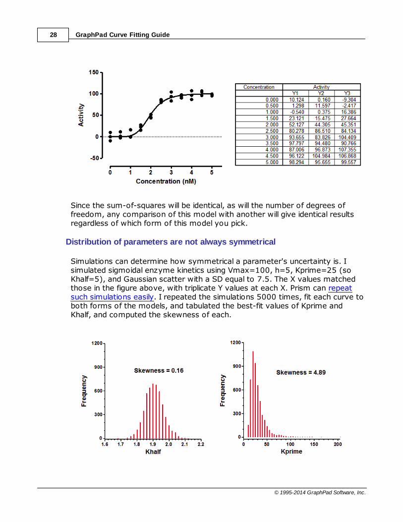
GraphPad Curve Fitting Guide28
© 1995-2014 GraphPad Software, Inc.
Since the sum-of-squares will be identical, as will the number of degrees offreedom, any comparison of this model with another will give identical resultsregardless of which form of this model you pick.
Distribution of parameters are not always symmetrical
Simulations can determine how symmetrical a parameter's uncertainty is. Isimulated sigmoidal enzyme kinetics using Vmax=100, h=5, Kprime=25 (soKhalf=5), and Gaussian scatter with a SD equal to 7.5. The X values matchedthose in the figure above, with triplicate Y values at each X. Prism can repeatsuch simulations easily. I repeated the simulations 5000 times, fit each curve toboth forms of the models, and tabulated the best-fit values of Kprime andKhalf, and computed the skewness of each.

PRINCIPLES OF CURVE FITTING 29
© 1995-2014 GraphPad Software, Inc.
Clearly the distribution of Khalf is quite symmetrical, and looks Gaussian. Theskewness is close to zero, as expected for a symmetrical distribution. Incontrast, the distribution of Kprime is quite skewed. Note that a few of thesimulations had best-fit values of Kprime greater than 100. The skewness value(4.89) confirms what is obvious by inspection -- the distribution is far fromsymmetrical.
Consequence of asymmetrical parameters
Ideally, a confidence interval is easy to interpret. A 95% CI has a 95% chanceof including the true population value of the parameter, and a 5% chance ofmissing it.
When analyzing real data, we never know the value of the true parameter, sonever know if the interval includes it or not. But when you simulate data, youknow the true values of the parameters, so can quantify the coverage of theconfidence intervals. I set up the same simulations mentioned above, fit eachdata set to both equations, and tabulated whether each confidence intervalincluded the true parameter value or not. This table shows the fraction of 5,000 simulations where the confidence interval did not include the trueparameter value (25 for Kprime, and 1.9037 for Khalf).
"95% CI" "99% CI"
Ideal5.0% 1.0%
Kprime8.8% 4.8%
Khalf5.1% 1.0%
These results show that Khalf is well behaved, as expected given its symmetry(see above). The 95% confidence interval is expected to miss the true value in5.0% of the simulations. In fact, it happened 5.1% of the time. Similarly, the99% CI is expected to miss the true value in 1.0% of the simulations, which isexactly what happened. In contrast, Kprime is less well behaved. The intervalscomputed to be 95% confidence intervals were not wide enough so missed thetrue value in 8.8% of the simulations. The 99% intervals were similarly not wideenough so missed the true value in 4.8% of the simulations. Thus the confidence intervals computed to be 99% intervals, actually turned out to be95% intervals.
These simulations show the advantage of choosing the equation that fits Khalf,rather than the one that fits Kprime. Khalf has a symmetrical distribution so theconfidence intervals computed from these fits can be interpreted at face value.

GraphPad Curve Fitting Guide30
© 1995-2014 GraphPad Software, Inc.
In contrast, Kprime has an asymmetrical distribution and its confidence intervalscannot be interpreted at face value.
One way to choose is to match other text books and papers, so your resultscan easily be compared to others. Another approach is to choose the form thatfits the way you think. If you prefer to think graphically, choose the Khalf. If youthink mechanistically, choose Kprime.
But the choice is more than a matter of convenience and convention. The restof this article explains how the choice of model determines the accuracy of theconfidence intervals.
1.4 Weighted nonlinear regression
Enter topic text here.
1.4.1 The need for unequal weighting in nonlinear regression
Both graphs above show dose-response curves, with response measured in tenreplicate values at each response. In the left graph, the standard deviation ofthose replicates is consistent. It is about the same all the way along the curve.In the right graph, the standard deviation of the replicates is related to the valueof Y. As the curve goes up, variation among replicates increases.

PRINCIPLES OF CURVE FITTING 31
© 1995-2014 GraphPad Software, Inc.
These data are simulated. In both cases, the scatter among replicates issampled from a Gaussian distribution. In the graph on the left, the SD of thatGaussian distribution is the same for all doses. On the right, the SD is aconstant fraction of the mean Y value. When a response is twice as high asanother response, the standard deviation among replicates is also twice aslarge. In other words, the coefficient of variation (CV) is constant.
What happens if you fit a model to the data on the right without taking intoaccount the fact that the scatter increases as Y increases? Consider two dosesthat give different responses that differ by a factor of two. The averagedistance of the replicates from the true curve will be twice as large for thehigher response. Since regression minimizes the sum of the squares of thosedistances those points will be expected to contribute four times as much to thesum-of-squares as the points with the smaller average Y value. In other words,the set of replicates whose average Y value is twice that of another set will begiven four times as much weight. This means, essentially, that the curve fittingprocedure will work harder to bring the curve near these points, and relativelyignore the points with lower Y values. You'd need to have four times as manyreplicates in the lower set to equalize the contribution to the sum-of-squares.
The goal of weighting is for points anywhere on the curve to contribute equallyto the sum-of-squares. Of course random factors will give some points morescatter than others. But the goal of weighting is to make those differences beentirely random, not related to the value of Y. The term weight is a bitmisleading, since the goal is to remove that extra weight from the points withhigh Y values. The goal is really to unweight.
Prism offers six choices on the Weights tab of nonlinear regression.
Prism file with graphs
1.4.2 Math theory of weighting
Relative weighting (weighting by 1/Y2)
In many experimental situations you expect the average distance (or ratherthe average absolute value of the distance) of the points from the curve to behigher when Y is higher. Another way to say this is that you expect thestandard deviation of the residuals (distance of points from the curve) to getlarger when Y is higher -- for the standard deviation to be proportional to thevalue of Y. Yet another way to say this is that you expect the coefficient ofvariation to be constant, but for the SD to not be constant.
If the SD of residuals is related to the value of Y, then the points with larger Yvalues will tend to be further from the curve (have larger residuals). These
160

GraphPad Curve Fitting Guide32
© 1995-2014 GraphPad Software, Inc.
points will therefore contribute more to the sum-of-squares, and thus dominatethe calculations.
The solution is not to minimize the sum-of-squares, but rather to minimize theweighted sum-of-squares. In other words, minimize the relative distances ofthe Y values of the data (Ydata) from the Y values of the curve (Ycurve). Whenyou choose relative weighting, nonlinear regression minimizes this quantity:
The left side is easiest to understand. For each point, compute how far it is (inthe Y direction) from the curve, divide that value by the Y value of the curve,and square that ratio. Add up that squared ratio for all points. The right side isequivalent. It squares the numerator and denominator separately, and thencomputes the ratio of those two squared values. This is the way mostmathematical statisticians think about weighting, so relative weighting is alsocalled weighting by Y2.
Poisson weighting
Weighting by 1/Y is a compromise between minimizing the actual distancesquared and minimizing the relative distance squared. One situation where 1/Yweighting is appropriate is when the Y values follow a Poisson distribution. Thiswould be the case when Y values are radioactive counts and most of thescatter is due to counting error. With the Poisson distribution, the standarderror of a value equals the square root of that value. Therefore you divide thedistance between the data and the curve by the square root of the value, andthen square that result. The equation below shows the quantity that Prismminimizes, and shows why it is called weighting by 1/Y (but Prism actuallyweights by the absolute value of Y.)
General weighting
The first three equations below shows how absolute, Poisson and relativeweighting are related. Note that taking anything to the zero power results in

PRINCIPLES OF CURVE FITTING 33
© 1995-2014 GraphPad Software, Inc.
1.0, so the denominator of equation on the left always equals 1.0.
The equation on the right shows general weighting. You enter K so cancustomize the weighting scheme to fit your data. Generally this choice is usedwith values of K between 1.0 and 2.0. Reference 1 below uses this approach.
If you want to experimentally determine the best value of K, you can do so:
1.Collect data with lots (over a dozen; maybe several dozen) replicates atmany points along the curve.
2.Plot the data the usual way to make sure the data seem correct.
3.Create a second graph that ignores the X values (time or concentration...).Instead, in this new graph, X is the logarithm of mean of the replicate Yvalues for each point on the first graph, and Y on this new graph is thelogarithm of variance (square of the standard deviation) among the replicatevalues. You can use either natural logarithms or logarithms base 10. Itdoesn't matter, so long as both logarithms uses the same base.
4.Fit a straight line to this graph using linear regression. Since the assumptionof a Gaussian variation around this line is dubious, use nonlinear regressionand choose a robust fit.
5.The slope of this regression line is K. If K is close to 0.0, then the SD doesnot vary with Y so no weighting is needed. If K is close to 2.0, then thestandard deviation is proportional to Y, and relative weighting is appropriate.If K is close to 1.0, choose Poisson weighting. If K has some other value, usegeneral weighting and enter this value of K as a constant.
Note that if Ycurve is negative, Prism actually takes the the absolute value ofYcurve to the K power.

GraphPad Curve Fitting Guide34
© 1995-2014 GraphPad Software, Inc.
Rarely used weighting choices in Prism
The choices to weight by 1/X or 1/X2 weight the points at the left part of thegraph more than points to the right. This is common in some fields when fittingstraight lines to bioassay data.
Prism also offers the choice to weight by the reciprocal of the standarddeviation squared. This option minimizes the following:
This method is most useful when you have formatted the data table for entryof SD values, but then entered values that you had calculated elsewhere basedon understanding how the scatter (or errors) arise in your experimentalsystem. The "SD" values you enter should be computed weighting factors, notthe actual SD of the data.
If you enter the actual SD into the SD subcolumn, or enter replicate values soPrism computes the SD, then Prism will use these actual SD values as weightingfactors. This is way less useful than it sounds. With small to moderate samplesizes, the SD will jump around a lot by chance, and it is not appropriate to usethese random SD values for weighting. Weighting should be by predicted SD notactual SD (which is subject to random factors).
Of course, weighting by SD is impossible if any of the entered SD values arezero. It also is impossible if Prism is computing the SD from replicates and thereis only one replicate, or if all replicates are identical (so their SD equals zero).
Reference
1. LM Lavasseur, H Faessel, HK SLocum, and WR Greco, Implications forClinical Pharmacodynamic Studies of the Statistical Characterization, of an InVitro Antiproliferation Assay, J. Pharmacokinetics and pharmacodynamics, 26:717-733, 1998.
Word file with equations

PRINCIPLES OF CURVE FITTING 35
© 1995-2014 GraphPad Software, Inc.
1.4.3 Don't use weighted regression with normalized data
Before fitting a log(dose) vs. response curve, it is common to first normalizethe data . This page explains why one should not use weighted regression inthis situation.
Weighted fits to nonnormalized data -- works great
The graph below shows simulated data that show a common situation. Thescatter among replicates is greater when the Y values are greater. In fact, thesedata were simulated so the SD among replicates is proportional to the Y value.
These data fit nicely using relative weighting. This minimizes the sum of thesquares of the relative distance between the points and the curve. In otherwords it minimizes:
I ran 10,000 simulations, and found that in every case the fit worked well andgave a reasonable answer (with the EC50 within the range of the data). Nosurprise so far. The data were fitting assuming a model that exactly matchedthe method used to simulate the data, and those fits worked well.
243

GraphPad Curve Fitting Guide36
© 1995-2014 GraphPad Software, Inc.
Weighted fits to normalized data -- ugh
People often like to normalize dose-response data so the Y values range from0% to 100%. What happens if these normalized data are fit with weightednonlinear regression?
I answered that question with simulations. Of 1,000 simulated data sets, 223could not be fit at all. Moreover, 60 simulated data sets gave nonsense results,with the EC50 outside of the range of the data. The remaining 72% of thesimulations seemed ok, but the confidence intervals were very wide in some.
What's going on?
With the data that were not normalized, the Y value of the best-fit curve at X =-4 is 3.05 times larger than the Y value of the curve at X=-8. Since theweighting is proportional the the Y value of the curve squared, the points nearthe top of the curve (at X=-4) get 3.052 , or 9.28, times as much weight aspoints near the bottom of the curve (at X=-8).
The situation is very different with the normalized data. With the first simulateddata set, the Y value of the best-fit curve at X = -4 is 17.77 times larger thanthe Y value of the curve at X=-8. Since the weighting is proportional the the Yvalue of the curve squared, the points near the top of the curve (at X=-4) get17.772 , or 315.8, times as much weight as points near the bottom of thecurve (at X=-8). Since the points at the top of the curve gets so much moreweight that those at the bottom, those at the bottom are essentially ignored,making the entire curve fit not work very well.
Another problem. Some of the Y values near the bottom of the normalizeddata sets are negative. Weighting factors really don't make any sense at allwhen some values are negative and some are positive.

PRINCIPLES OF CURVE FITTING 37
© 1995-2014 GraphPad Software, Inc.
In summary: After normalizing the SD among replicates is no longerproportional to the Y values, so relative weighting is not appropriate.
Bottom line
The whole idea of weighted nonlinear regression is to match the weightingscheme used by the regression to the variation in the actual data. If younormalize the data, none of the usual weighting schemes will work well.
If you really want to show your data on a normalized axis running from 0% to100%, you can do so. First fit the model to the actual data using anappropriate weighting scheme. Then normalize both the data and the curve.
Details and link to Prism file
1.4.4 What are the consequences of choosing the wrong weighting method
What happens if you leave the choice on the weighting tab set to its default --no weighting -- when the scatter is actually related to the Y value? Of course,the answer is "it depends"? It depends on how large the scatter is, and howlarge a range the Y values span. The rest of this article looks at one example,and simulates many data sets to see what happens when the fitting is doneinappropriately.
Simulations
I picked a very simple model -- a straight line. I simulated the data so the SD ofscatter at any point along the line is proportional to the Y value of that point.The graph below shows a simulated data set. You can clearly see that thescatter among replicates increases as the line goes up.

GraphPad Curve Fitting Guide38
© 1995-2014 GraphPad Software, Inc.
The line was fit to the data by "nonlinear" regression. Prism does not offerdifferential weighting as part of its linear regression analysis, but "nonlinear"regression can fit a straight line with many options not available in the linearregression analysis .
The red line used the default choice -- no weighting; minimize sum of squares.The blue line used relative weighting. This choice is appropriate when you expectthe SD of replicate residuals to be proportional to Y. The two lines are notidentical.
I simulated 5000 such data sets using the Monte Carlo analysis of Prism 6.Each of the 5000 simulated data sets was fit with both unweighted andweighted (relative weighting) regression. I recorded both the best-fit value ofthe slope and its standard error (SE) for both analyses of each of the 5000data sets.
82

PRINCIPLES OF CURVE FITTING 39
© 1995-2014 GraphPad Software, Inc.
The scatter among replicates was proportional to Y, so relative weighting isappropriate. The results of these simulations are shown in blue. The results inred show the results when the regression used equal weighting (the default).The boxes extend from the 25th to the 75th percentile, with a line at themedian (50th percentile). The whiskers extend down to the smallest value andup to the largest.
The left graph above shows the distribution of the best-fit values of the slopes.Chossing the wrong weighting scheme would not systematically result in abest-fit value of slope that is too high (too steep) or too low (too shallow).Indeed, the median best-fit values for slope are almost identical for the no-weighting and relative-weighting fits. But note that the results with no weighting has a much broader spread of slopes. Since these are simulated data, weknow the true slope (1.0) and can quantify how far the best-fit slope is fromthat idea for each simulated data set. The median error when the data were fitwithout differential weighting (red) was 0.04610, compared to 0.02689 for thesimulations with relative weighting (blue).In this example, choosing the wrongweighting scheme increased the median error by 71%.
The graph on the right above shows the distribution of the SE of the slopes. TheSE of the slope is much higher on average and less consistent (wider spread) when the fits were done with equal weighting for all points. The median SE forthe unweighted fits was 73% larger than the median SE for the weighted fits.Since the width of the confidence interval is proportional to the SE, this meansthe median confidence interval was 73% wider when the fits were done withoutweighting.

GraphPad Curve Fitting Guide40
© 1995-2014 GraphPad Software, Inc.
Since these are simulated data, we know the true population slope (it is 1.0).So we can ask for each simulation whether the reported 95% confidenceinterval included the true value. For the relative weighting simulations, the 95%confidence intervals included the true value in 95.3% of the simulated data sets.When those same data sets were analyzed without weighting, only 92.6% ofthe "95%" confidence intervals included the true value.
Summary
In summary, when we chose the wrong weighting scheme in this example:
The best-fit value of the slope was less precise.
The SE of the slope was larger, and thus the confidence intervals were wider.
Even though the 95% confidence intervals were wider, they weren't wide
enough. The "95%" confidence interval only included the true value in fewerthan 95% of the simulations.
This is just one example. With other examples, the choice of weighting methodmatters less. But with still other examples, it may matter more. It is worthtrying to choose the appropriate weighting scheme.
Download the Prism file for this example.
1.5 The many uses of global nonlinear regression
A global model defines a family of curves, rather than just asingle curve, with some parameters shared between data sets.For each shared parameter, Prism fits one (global) best-fit valuethat applies to all the data sets. For each non-sharedparameter, Prism fits a separate (local) best-fit value for eachdata set.
What is global nonlinear regression?
Using global regression to fit incompletedatasets
Fitting models where the parameters aredefined by multiple data sets
41
42
43

PRINCIPLES OF CURVE FITTING 41
© 1995-2014 GraphPad Software, Inc.
Advice: Don't use global regression if datasetsuse different units
1.5.1 What is global nonlinear regression?
A global model defines a family of curves, rather than just a single curve. Someparameters are shared so a single parameter value applies to all the curves,while other parameters apply to each data individually. For each sharedparameter, fit one (global) best-fit value that applies to all the data sets. Foreach non-shared parameter, fit a separate (local) best-fit value for each dataset.
Nonlinear regression finds parameters of a model that make the curve come asclose as possible to the data. This is done by minimizing the sum of the squaresof the vertical distances between the data points and curve. Global nonlinearregression extends this idea to fitting several data sets at once and minimizesthe sum (of all data sets) of sum (of all data points) of squares.
Prism makes it very easy to perform global nonlinear regression. Enter yourdata on one data table, click analyze, choose nonlinear regression and choose amodel. On the Constrain tab of the Nonlinear regression dialog, choose whichparameter(s) to share among data sets.
1.5.2 The uses of global nonlinear regression
Global nonlinear regression is useful in (at least) three situations:
Test whether a parameter value differs significantly between data sets.
Compare the sum-of-squares (to assess goodness-of-fit) when theparameter is shared, with the sum of the sum-of-squares when theparameter is fit individually to each dataset. In Prism, set up this kind ofcomparison in the Compare tab .
Fit families of data where each dataset is incomplete, but the entire family
of datasets defines the parameters. For example, one data set may do agreat job of defining the bottom plateau of a dose-response curve, whileanother data set defines the top. Fit the two data sets separately, and theresults may be ambiguous (very wide confidence intervals). Globally fit bothcurves, and the results might be very tight. See an example .
Fit models where the parameter(s) you care about cannot be determined
from any one dataset, but only from the relationship between several datasets . Another example is fitting enzyme inhibition data .
45
158
158
42
43 345
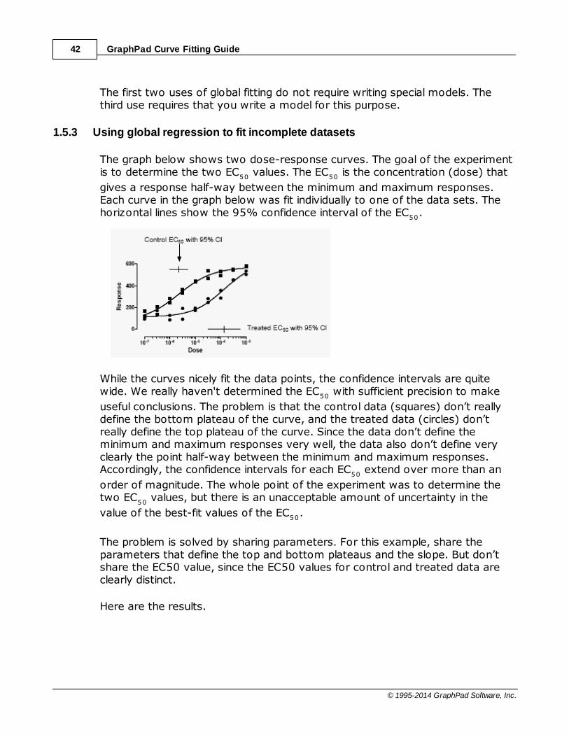
GraphPad Curve Fitting Guide42
© 1995-2014 GraphPad Software, Inc.
The first two uses of global fitting do not require writing special models. Thethird use requires that you write a model for this purpose.
1.5.3 Using global regression to fit incomplete datasets
The graph below shows two dose-response curves. The goal of the experimentis to determine the two EC
50 values. The EC
50 is the concentration (dose) that
gives a response half-way between the minimum and maximum responses.Each curve in the graph below was fit individually to one of the data sets. Thehorizontal lines show the 95% confidence interval of the EC
50.
While the curves nicely fit the data points, the confidence intervals are quitewide. We really haven't determined the EC
50 with sufficient precision to make
useful conclusions. The problem is that the control data (squares) don’t reallydefine the bottom plateau of the curve, and the treated data (circles) don’treally define the top plateau of the curve. Since the data don’t define theminimum and maximum responses very well, the data also don’t define veryclearly the point half-way between the minimum and maximum responses.Accordingly, the confidence intervals for each EC
50 extend over more than an
order of magnitude. The whole point of the experiment was to determine thetwo EC
50 values, but there is an unacceptable amount of uncertainty in the
value of the best-fit values of the EC50
.
The problem is solved by sharing parameters. For this example, share theparameters that define the top and bottom plateaus and the slope. But don’tshare the EC50 value, since the EC50 values for control and treated data areclearly distinct.
Here are the results.

PRINCIPLES OF CURVE FITTING 43
© 1995-2014 GraphPad Software, Inc.
The graph of the curves looks only slightly different. But now the program findsthe best-fit parameters with great confidence. The 95% confidence intervals forthe EC
50 values span about a factor of two (compared to a factor of ten or
more when no parameters were shared).
The control data define the top of the curve pretty well, but not the bottom.The treated data define the bottom of the curve pretty well, but not the top. Byfitting both data sets at once, sharing some parameters, both EC50 valueswere determined with reasonable certainty.
1.5.4 Fitting models where the parameters are defined by multiple data sets
Global fitting is most useful when the parameters you care most about arenot defined by any one data set, but rather by the relationship between twodata sets.
Sample data
Choose the XY sample data set: Binding --Saturation binding to total andnonspecific
Fit the data using nonlinear regression, open the "Binding --Saturation" list ofequations, and choose "One site -- total and nonspecific". You'll see the fitbelow.

GraphPad Curve Fitting Guide44
© 1995-2014 GraphPad Software, Inc.
Explanation of the equation and global fitting
This experiment measured equilibrium binding of radioligand at variousconcentrations of radioligand to find the B
max and K
d of the radioligand. Since the
ligand binds to nonspecific sites as well as the receptor of interest, theexperiment measured both total binding and nonspecific binding (binding ofradioligand in the presence of an excess of an unlabeled receptor blocker).
These kind of data are often analyzed by first subtracting the nonspecific bindingfrom the total binding. The resulting specific binding is then fit to a model thatdescribes equilibrium binding to one receptor site.
Global fitting simultaneously fits both the total binding and the nonspecificbinding. There is no need to first subtract the two data sets. The only trick is towrite a model that fits different equations to each data set. Prism's built inequation is set up as follows:
specific=Bmax*X/(X+Kd)nonspecific=NS*X + Background<A>Y=specific+nonspecific<B>Y=nonspecific
The first line defines specific saturable binding.
The second line defines nonspecific binding to be a constant fraction of addedradioligand (X) plus a background (which is often zero).
The third line is preceded by <A>, so it only applies to the first data set (column

PRINCIPLES OF CURVE FITTING 45
© 1995-2014 GraphPad Software, Inc.
A, total binding). It defines the Y values in that dataset to equal the sum of totaland nonspecific binding.
The fourth line is preceded by <B> so only applies to the second data set, anddefines those Y values to equal nonspecific binding.
The equation is defined with the constraint that the parameters NS andbackground are shared between the two data sets. That way, Prism finds onebest-fit value for NS and background, based on fitting both data sets. SinceBmax and Kd are only used in fitting the first dataset, it wouldn't be meaningfulto share these parameters.
The parameters you care about (Bmax and Kd) cannot be determined preciselyby fitting just one dataset. But fitting a model that defines both data sets (andtheir relationship) while sharing the parameter NS between the datasets, letsPrism get the most information possible from the data.
1.5.5 Advice: Don't use global regression if datasets use different units
Global fitting works by minimizing the sum (for all data sets) of the sum (for alldata points) of squares of distances of the data points from the curve. Thisapproach only makes sense when all the data are expressed in the same units.
If different data sets are expressed in different units, be very cautious aboutusing global fitting. The problem is that your decision about which units to usecan change the results.
For example, imagine what happens if you change one data set fromexpressing weight in grams to expressing weight in milligrams. All the values arenow increased by a factor of one thousand, and the sum-of-squares for thatdata set is increased by a factor of one million (one thousand squared).Compared to other data sets, expressed in different units, this data set nowhas a much greater impact on the fit. If you really need to do global fit to datasets using different units, consider first normalizing the data so they arecomparable.
1.6 Comparing fits of nonlinear models
When fitting a nonlinear model to data, your main objective isoften to discriminate between different models, or to askwhether an experimental intervention changed a parameter.
Comparing models can answer four distinct

GraphPad Curve Fitting Guide46
© 1995-2014 GraphPad Software, Inc.
questions :
For each data set, which of two equations(models) fits best?
Do the best-fit values of selectedunshared parameters differ between datasets?
For each dataset, does the best-fit valueof a parameter differ from a theoreticalvalue?
Does one curve adequately fit all the data
Prism lets you choose from two approaches tocomparing models : the extra sum-of-squaresF tests and the AICc approach based oninformation theory.
How the F test works to compare models
How the AICc computations work
The idea of comparing models extends waybeyond nonlinear regression. In fact, much ofstatistics can be viewed as comparing models
1.6.1 Questions that can be answered by comparing models
When fitting data with regression, in many cases your main objective may be tocompare the fits of different models, or to ask if an experimental interventionchanged a parameter.
On the Compare tab of the Nonlinear regression dialog, Prism offers fourchoices:
For each data set, which of two equations (models) fits best?
Compare the fit of two models, taking into account differences in the number of
46
48
50
51
157
PRINCIPLES OF CURVE FITTING 47
© 1995-2014 GraphPad Software, Inc.
parameters to be fit. Most often, you will want to compare two relatedequations. Comparing the fits of two unrelated equations is rarely helpful.
Example: Compare a one-phase exponential decay with a two-phaseexponential decay.
Do the best-fit values of selected unshared parameters differ between data sets?
Compare the fit when the selected parameter(s) are shared among all datasetswith the fit when those parameter(s) are fit individually to each dataset.
If you pick one parameter, you are asking whether the best-fit value of thatone parameter differs among datasets.
If you pick all the parameters, you are asking whether a single curve adequatelyfits all the data points, or if you get a better fit with individual curves for eachdataset.
Example: Fit a family of dose-response curves and compare the fit when theslope factor (Hill slope) is shared with the fit when each curve is fit individually.This is a way to test whether the curves are parallel.
For each dataset, does the best-fit value of a parameter differ from a theoreticalvalue?
You may have theoretical reasons to believe that a parameter will have acertain value (often 0.0, 100, or 1.0). Compare the fit when the parameter isconstrained to that value with the unconstrained fit.
Example: Test if a Hill Slope differs from 1.0 (a standard value).
Does one curve adequately fit all data sets?
This choice compares the fits of separate curves to each data set with the fit ofa single curve fit to all the data sets. It asks whether there is evidence that thetreatments did anything to shift the curves.
This choice is new in Prism 6 and is identical to choosing "Do the best-fit valuesof selected unshared parameters differ between data sets?" and then selectingall the parameters.

GraphPad Curve Fitting Guide48
© 1995-2014 GraphPad Software, Inc.
1.6.2 Approaches to comparing models
Approach to comparing models
Which model is 'best'? At first, the answer seems simple. The goal of nonlinearregression is to minimize the sum-of-squares, so it seems as though the modelwith the smaller sum-of-squares is best. If the two alternative models bothhave the same numbers of parameters, then indeed that is the best approach.
But that approach is too simple when the models have different numbers ofparameters, which is usually the case. A model with more parameters can havemore inflection points, so of course comes closer to the points. It can bend andtwist more to get near the data points. Accordingly, a two-phase model almostalways fits better than a one-phase model, and a three-phase model fits evenbetter. So any method to compare a simple model with a more complicatedmodel has to balance the decrease in sum-of-squares with the increase in thenumber of parameters.
Two statistical approaches to comparing models
Prism offers two approaches to comparing models with different numbers ofparameters. These are not the only methods that have been developed tosolve this problem, but are the most commonly used methods.
Extra sum-of-squares F test
The Extra sum-of-squares F test is based on traditional statistical hypothesistesting.
The null hypothesis is that the simpler model (the one with fewer parameters)is correct. The improvement of the more complicated model is quantified as thedifference in sum-of-squares. You expect some improvement just by chance,and the amount you expect by chance is determined by the number of datapoints and the number of parameters in each model. The F test compares thedifference in sum-of-squares with the difference you would expect by chance.The result is expressed as the F ratio, from which a P value is calculated.
The P value answers this question:
If the null hypothesis is really correct, in what fraction of experiments (thesize of yours) will the difference in sum-of-squares be as large as youobserved, or even larger?
If the P value is small, conclude that the simple model (the null hypothesis) iswrong, and accept the more complicated model. Usually the threshold P value
50

PRINCIPLES OF CURVE FITTING 49
© 1995-2014 GraphPad Software, Inc.
is set at its traditional value of 0.05. If the P value is less than 0.05, then youreject the simpler (null) model and conclude that the more complicated modelfits significantly better.
Information theory approach Akaike's criterion (AIC)
This alternative approach is based on information theory, and does not use thetraditional “hypothesis testing” statistical paradigm. Therefore it does notgenerate a P value, does not reach conclusions about “statistical significance”,and does not “reject” any model.
The method determines how well the data supports each model, taking intoaccount both the goodness-of-fit (sum-of-squares) and the number ofparameters in the model. The results are expressed as the probability that eachmodel is correct, with the probabilities summing to 100%. If one model is muchmore likely to be correct than the other (say, 1% vs. 99%), you will want tochoose it. If the difference in likelihood is not very big (say, 40% vs. 60%), youwill know that either model might be correct, so will want to collect more data. How the calculations work .
Which approach to choose?
In most cases, the models you want to compare will be 'nested'. This meansthat one model is a simpler case of the other. For example, a one-phaseexponential model is a simpler case of a two-phase exponential model. A threeparameter dose-response curve with a standard Hill slope of 1.0 is a specialcase of a four parameter dose-response curve that finds the best-fit value ofthe Hill slope as well.
If the two models are nested, you may use either the F test or the AICapproach. The choice is usually a matter of personal preference and tradition.Basic scientists in pharmacology and physiology tend to use the F test.Scientists in fields like ecology and population biology tend to use AIC approach.
If the models are not nested, then the F test is not valid, so you should choosethe information theory approach. Note that Prism does not test whether themodels are nested.
How do these methods work to compare data sets?
The Compare tab of Prism lets you ask "Do the best-fit values of selectedunshared parameters differ between data sets?" or "Does one curveadequately fit all data sets?". Applying the F test or Akaike's method toanswering these questions is straightforward. Prism compares the sum-of-squares of two fits.
51
157

GraphPad Curve Fitting Guide50
© 1995-2014 GraphPad Software, Inc.
In one fit, the model is separately fit to each data set, and the goodness-of-fit
is quantified with a sum-of-squares. The sum of these sum-of-square valuesquantifies the goodness of fit of the family of curves fit to all the data sets.
The other fit is a global fit to all the data sets at once, sharing specified
parameters. If you ask Prism whether one curve adequately fits all data sets,then it shares all the parameters.
These two fits are nested (the second is a simpler case of the first, with fewerparameters to fit) so the sums-of-squares (actually the sum of sum of squaresfor the first fits) can be compared using either the F test or Akaike's method
.
Interpreting comparison of models
1.6.3 How the F test works to compare models
If the simpler model is correct, the relative increase in the sum of squares(going from more complicated to simpler model) is expected to equal therelative increase in degrees of freedom. In other words, if the simpler model iscorrect you expect that:
SS1 is the sum-of-squares for the simpler model (which will be higher) and SS2is the sum-of-squares of the more complicated model.
If the more complicated model is correct, then you expect the relative increasein sum-of-squares (going from complicated to simple model) to be greater thanthe relative increase in degrees of freedom:
The F ratio quantifies the relationship between the relative increase in sum-of-squares and the relative increase in degrees of freedom.
50
51
212

PRINCIPLES OF CURVE FITTING 51
© 1995-2014 GraphPad Software, Inc.
That equation is more commonly shown in an equivalent form:
F ratios are always associated with a certain number of degrees of freedom forthe numerator and a certain number of degrees of freedom for thedenominator. This F ratio has DF1-DF2 degrees of freedom for the numerator,and DF2 degrees of freedom for the denominator.
If the simpler model is correct you expect to get an F ratio near 1.0. If the ratiois much greater than 1.0, there are two possibilities:
The more complicated model is correct.
The simpler model is correct, but random scatter led the more complicated
model to fit better. The P value tells you how rare this coincidence would be.
The P value answers this question:
If model 1 is really correct, what is the chance that you would randomlyobtain data that fits model 2 so much better?
If the P value is low, conclude that model 2 is significantly better than model 1.Otherwise, conclude that there is no compelling evidence supporting model 2,so accept the simpler model (model 1).
1.6.4 How the AICc computations work
While the theoretical basis of Akaike's method is difficult to follow, it is easy todo the computations and make sense of the results.
The fit of any model to a data set can be summarized by an informationcriterion developed by Akaike, called the AIC. If you accept the usualassumptions of nonlinear regression (that the scatter of points around thecurve follows a Gaussian distribution), the AIC is defined by a simple equationfrom the sum-of-squares and number of degrees of freedom of the twomodels. It is not possible to make sense of this AIC value itself, because itsunits depend on which units you use for your data.
To compare models, it is only the difference between the two AIC values thatmatter. When you take the difference, the units cancel out and the result isunitless.

GraphPad Curve Fitting Guide52
© 1995-2014 GraphPad Software, Inc.
SS2∆AIC = N×ln +2 DF
SS1
The equation now makes intuitive sense. Like the F test, it balances the changein goodness-of-fit as assessed by sum-of-squares with the change in thenumber of degrees of freedom (due to differences in the number of parametersto be fit). Since model 1 is the simpler model, it will almost always fit worse, soSS1 will be greater than SS2. Since the logarithm of a fraction is alwaysnegative, the first term will be negative. Model 1 has fewer parameters and sohas more degrees of freedom, making the last term positive. If the net result isnegative, that means that the difference in sum-of-squares is more thanexpected based on the difference in number of parameters, so you concludethat the more complicated model is more likely.
Prism reports the difference between the two AICc values as the AICc of thesimpler model minus the AICc of the more complicated model. When the morecomplicated (more parameters) model has the lower AICc and so is preferred,Prism reports the difference of AICc as a positive number. When the simplermodel has the lower AICc and so is preferred, Prism reports the difference ofAICc as a negative number.
The equation above helps you get a sense of how AIC works – balancingchange in goodness-of-fit vs. the difference in number of parameters. But youdon’t have to use that equation. Just look at the individual AIC values, andchoose the model with the smallest AIC value. That model is most likely to becorrect.
Prism actually doesn't report the AIC, but rather the AICc. That value includes acorrection for low sample size. The equation is a bit more complicated, and ismore accurate with small sample size. With larger sample sizes, the AIC andAICc are almost the same.
Note that these calculations are based on information theory, and do not usethe traditional “hypothesis testing” statistical paradigm. Therefore there is no Pvalue, no conclusion about “statistical significance”, and no “rejection” of amodel.
From the difference in AICc values, Prism calculates and reports the probabilitythat each model is correct, with the probabilities summing to 100%. If onemodel is much more likely to be correct than the other (say, 1% vs. 99%), youwill want to choose it. If the difference in likelihood is not very big (say, 40% vs.60%), you will know that either model might be correct, so will want to collectmore data.
Note that this method simply compares the fits of the two models you chose.

PRINCIPLES OF CURVE FITTING 53
© 1995-2014 GraphPad Software, Inc.
It is possible that a third model, one you didn't choose, fits far better thaneither model you chose.
1.7 Outlier elimination and robust nonlinear regression
Nonlinear regression, like linear regression, assumes that thescatter of data around the ideal curve follows a Gaussian ornormal distribution. Outliers can violate this assumption andinvalidate nonlinear regression results. To deal with outliers,Prism offers robust regression and automatic outlier removal.
What are the advantages of removing outliers.But isn't it cheating?
Outlier removal has to be used carefully. Itmust be avoided in many situations.
Once you've identified an outlier, beware orremoving it from graphs and analyses. Anoutlier is not always a 'bad' point.
Prism uses an outlier removal method createdby GraphPad Software --the ROUT method. Learn how it works.
When identifying outliers, the step is to fit acurve using a robust method designed sooutliers won't affect the curve much. Learnabout robust nonlinear regression.
1.7.1 When to use automatic outlier removal
The problem with outliers
Nonlinear regression, like linear regression, assumes that the scatter of dataaround the ideal curve follows a Gaussian or normal distribution. Thisassumption leads to the familiar goal of regression: to minimize the sum of thesquares of the vertical or Y-value distances between the points and the curve.However, experimental mistakes can lead to erroneous values – outliers. Evena single outlier can dominate the sum-of-the-squares calculation, and lead tomisleading results.
53
54
56
57
59
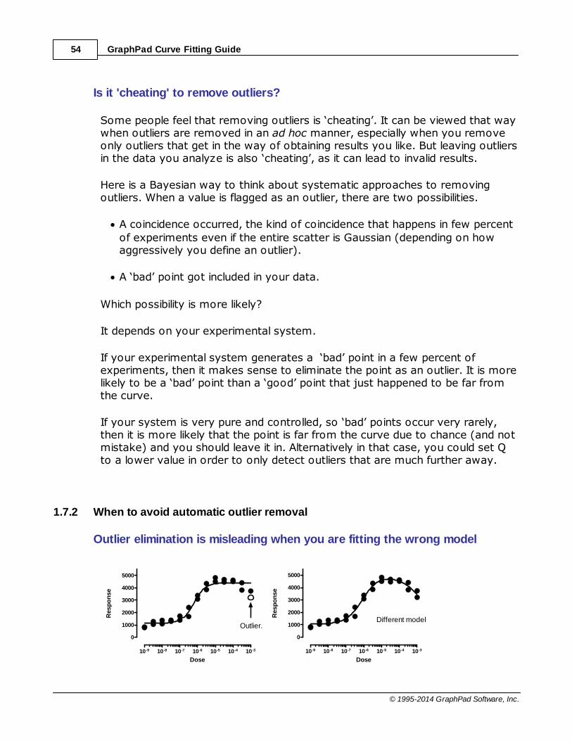
GraphPad Curve Fitting Guide54
© 1995-2014 GraphPad Software, Inc.
Is it 'cheating' to remove outliers?
Some people feel that removing outliers is ‘cheating’. It can be viewed that waywhen outliers are removed in an ad hoc manner, especially when you removeonly outliers that get in the way of obtaining results you like. But leaving outliersin the data you analyze is also ‘cheating’, as it can lead to invalid results.
Here is a Bayesian way to think about systematic approaches to removingoutliers. When a value is flagged as an outlier, there are two possibilities.
A coincidence occurred, the kind of coincidence that happens in few percent
of experiments even if the entire scatter is Gaussian (depending on howaggressively you define an outlier).
A ‘bad’ point got included in your data.
Which possibility is more likely?
It depends on your experimental system.
If your experimental system generates a ‘bad’ point in a few percent ofexperiments, then it makes sense to eliminate the point as an outlier. It is morelikely to be a ‘bad’ point than a ‘good’ point that just happened to be far fromthe curve.
If your system is very pure and controlled, so ‘bad’ points occur very rarely,then it is more likely that the point is far from the curve due to chance (and notmistake) and you should leave it in. Alternatively in that case, you could set Qto a lower value in order to only detect outliers that are much further away.
1.7.2 When to avoid automatic outlier removal
Outlier elimination is misleading when you are fitting the wrong model
10 -9 10-8 10-7 10-6 10-5 10 -4 10 -3
0
1000
2000
3000
4000
5000
Outlier.
Dose
Resp
on
se
10 -9 10 -8 10-7 10-6 10 -5 10 -4 10-3
0
1000
2000
3000
4000
5000
Different model
Dose
Resp
on
se

PRINCIPLES OF CURVE FITTING 55
© 1995-2014 GraphPad Software, Inc.
The left panel above shows the data fit to a dose response curve . In thisfigure, one of the points is a significant outlier. But this interpretation assumesthat you’ve chosen the correct model. The right panel shows the data fit to analternative bell-shaped dose-response model , where high doses evoke asmaller response than does a moderate dose. The data fit this model very well,with no outliers detected (or even suspected).
This example points out that outlier elimination is only appropriate when youare sure that you are fitting the correct model.
Outlier elimination is misleading when data points are not independent
10 -9 10 -8 10 -7 10 -6 10 -5 10 -4 10 -3
0
2500
5000
7500Outlier
Dose
Resp
on
se
10 -9 10 -8 10 -7 10 -6 10 -5 10 -4 10 -3
0
2500
5000
7500
Dose
Resp
on
se
The left panel above show data fit to a dose-response model with one point (inthe upper right) detected as an outlier. The right panel shows that the datareally come from two different experiments. Both the lower and upper plateausof the second experiment (shown with upward pointing triangles) are higherthan those in the first experiment (downward pointing triangles). Because theseare two different experiments, the assumption of independence was violated inthe analysis in the left panel. When we fit each experimental run separately, nooutliers are detected.
Outlier elimination is misleading when you chose incorrect weighting factors
10 -9 10 -8 10 -7 10 -6 10 -5 10-4 10 -3
0
1000
2000
3000
4000
5000
6000
Four Outliers
Dose
Resp
on
se
-9 -8 -7 -6 -5 -4 -3
0
1000
2000
3000
4000
5000
6000
Dose
Resp
on
se
The left panel above shows data fit to a dose-response model. Four outlierswere identified (two are almost superimposed). But note that the values withlarger responses (Y values) also, on average, are further from the curve. This
256
271

GraphPad Curve Fitting Guide56
© 1995-2014 GraphPad Software, Inc.
makes least-squares regression inappropriate. To account for the fact that theSD of the residuals is proportional to the height of the curve, we need to use weighted regression . The right panel shows the same data fit to the samedose-response model, but minimizing sum of the squares of the distance of thepoint from the curve divided by the height of the curve, using relative weighting.Now no outliers are identified. Using the wrong weighting method created falseoutliers.
1.7.3 Outliers aren't always 'bad' points
Definition of an 'outlier'
The term 'outlier' is defined fairly vaguely, but refers to a value that is far fromthe others. In Prism's nonlinear regression, an outlier is a point that is far fromthe best-fit curve defined by robust regression.
Of course, there is some possibility that an outlier really comes from the sameGaussian population as the others, and just happens to be very high or low.You can set the value of Q to control how aggressively Prism definesoutliers.
Outliers are not always due to mistakes
Nonlinear regression is usually used with experimental data, where X is avariable like time or concentration or some other variable you manipulate in theexperiment. Since all the scatter is due to experimental error, it can makesense to eliminate any extreme outlier since it is almost certainly the result ofan experimental mistake.
In other situations, each data point can represent a different individual. In thiscase, an outlier may not be due to experimental mistakes, but rather be theresult of biological variation, or differences in some other variable that is notincluded in your model. Here, the presence of the outlier may be the mostinteresting finding in the study. While the ROUT outlier method might proveuseful to flag an outlier in this situation, it would be a big mistake toautomatically exclude such outliers without further thought (orexperimentation).
30
160

PRINCIPLES OF CURVE FITTING 57
© 1995-2014 GraphPad Software, Inc.
In quality control analyses, an outlier can tell you about a process that is out ofcontrol. You wouldn't want to delete outliers, without first figuring out why thevalue is far from the others. The outlier might be telling you somethingimportant.
1.7.4 The ROUT method of identifying outliers
How the ROUT method of removing outliers works
Prism offers a unique approach to identifying and removing outliers, detailed inreference 1.Because this method combines Robust regression and Outlierremoval, we call it the ROUT method.
The ROUT method of regression follows these steps.
1.Our robust nonlinear regression method is used to fit a curve that is notinfluenced by outliers.
2.The residuals of the robust fit are analyzed to identify any outliers. This stepuses a new outlier test adapted from the False Discovery Rate approach oftesting for multiple comparisons.
3.Remove the outliers, and perform ordinary least-squares regression on theremaining data.
How to use the ROUT method with Prism
Although the ROUT method requires three steps (listed above), Prism does allthis automatically. All you have to do is check an option on the Fit tab ofnonlinear regression dialog:
Prism then identifies the outliers, eliminates them, and fits the remaining points.The outliers are shown in a separate table, and the number of outliers istabulated on the main results table.
The ROUT coefficient Q
The value of Q determines how aggressively the ROUT method defines outliers.
59

GraphPad Curve Fitting Guide58
© 1995-2014 GraphPad Software, Inc.
The mathematical details are explained in reference 1. This value is set in the Weights tab of the Nonlinear regression dialog.
If you set Q to a higher value, the threshold for defining outliers is less strict.This means that Prism will have more power to detect outliers, but also willfalsely detect 'outliers' more often.
If you set Q to a lower value, the threshold for defining outliers is stricter. Thismeans that Prism will have a less power to detect real outliers, but also have asmaller chance of falsely defining a point to be an outlier.
Unless you have a strong reason to choose otherwise, we recommend stickingwith the default value of 1%. Our simulations have shown that if all the scatteris Gaussian, Prism will falsely find one or more outliers in about 2-3% ofexperiments. This does not mean that a few percent of all values are declaredto be outliers, but rather that one or more outliers will be detected in a fewpercent of experiments. If there really are outliers present in the data, Prism willdetect them with a False Discovery Rate less than 1%.
Unequal weighting, robust regression and outlier removal
As we explain in reference 1, unequal weighting is not useful with robustregression. The problem is that outliers can get way too much weight.
If you choose both unequal weighting and robust fitting, therefore, Prism doesthe fitting assuming equal weights. However it does use your weighting choicewhen creating a table of residuals.
If you choose both unequal weighting and automatic outlier removal, Prism firstfits using robust regression (ignoring your weighting choice). It does use theweighting factors when identifying the outliers, as explained in reference 1. Itthen performs weighted nonlinear regression on the outlier-depleted data.
Reference
1.Motulsky HM and Brown RE, Detecting outliers when fitting data withnonlinear regression – a new method based on robust nonlinear regressionand the false discovery rate, BMC Bioinformatics 2006, 7:123.
160

PRINCIPLES OF CURVE FITTING 59
© 1995-2014 GraphPad Software, Inc.
1.7.5 Robust nonlinear regression
The need for robust regression
Nonlinear regression, like linear regression, assumes that the scatter of dataaround the ideal curve follows a Gaussian or normal distribution. Thisassumption leads to the familiar goal of regression: to minimize the sum of thesquares of the vertical or Y-value distances between the points and the curve.This standard method for performing nonlinear (or linear regression) is called least-squares.
Experimental mistakes can lead to erroneous values whose values are way toohigh or too low– outliers. Even a single outlier can dominate the sum-of-the-squares calculation, and lead to misleading results. One way to cope with thisproblem is to perform a robust fit using a method that is not very sensitive toviolations of the Gaussian assumption. Another approach is to use automaticoutlier elimination to identify and remove the outliers, and then run least-squares regression. Prism offers both choices.
How robust regression works
Based on a suggestion in Numerical Recipes (1), we based our robust fittingmethod on the assumption that variation around the curve follows a Lorentziandistribution, rather than a Gaussian distribution. Both distributions are part of afamily of t distributions:
-6 -5 -4 -3 -2 -1 0 1 2 3 4 5 6
df= (Gaussian)
df=4
df=10
df=1 (Lorentzian or Cauchy)
Normalized distance of point from curve
The widest distribution in that figure, the t distribution for df=1, is also known asthe Lorentzian distribution or Cauchy distribution. The Lorentzian distributionhas wide tails, so outliers are fairly common and therefore have little impact onthe fit.
We adapted the Marquardt nonlinear regression algorithm to accommodatethe assumption of a Lorentzian (rather than Gaussian) distribution of residuals,
53
62

GraphPad Curve Fitting Guide60
© 1995-2014 GraphPad Software, Inc.
and explain the details in reference 2.
When does it make sense to choose robust nonlinear regression?
If your goal is just to obtain best-fit values of the parameters, robustregression works great. Outliers have little impact. Yet if all the data isGaussian, robust regression and least-squares regression give almost identicalresults
Robust regression (as implemented by Prism) has three drawbacks:
Robust regression cannot generate standard errors or confidence intervals
for the parameters.
Robust regression cannot generate confidence or prediction bands.
Robust regression cannot compare the fits of two models or two datasets.
The main use of robust regression in Prism is as a 'baseline' from which to remove outliers . Its inability to compute standard errors or confidenceintervals of the parameters greatly limits the usefulness of robust regression.We recommend it only to those who want to better understand the outlier-removal method (which begins with robust regression).
References
1. Press WH, Teukolsky SA, Vettering WT, Flannery BP: Numerical Recipes in C. the Artof Scientific Computing. New York, NY: Cambridge University Press; 1988.
2. Motulsky HM and Brown RE, Detecting outliers when fitting data with nonlinear regression– a new method based on robust nonlinear regression and the false discovery rate, BMCBioinformatics 2006, 7:123. Download as pdf.
1.8 How nonlinear regression works
If you want to really understand how nonlinear regressionworks, you will need to learn matrix algebra and study advancedmath books. But you can use nonlinear regression effectively solong as you understand the basic principles of regression.
Why minimize the sum-of-squares?
53
61

PRINCIPLES OF CURVE FITTING 61
© 1995-2014 GraphPad Software, Inc.
How nonlinear regression works
The need for unequal weighting in nonlinearregression
How standard errors and confidence intervalsare computed
How confidence and prediction bands arecomputed
Replicates
How dependency is calculated
1.8.1 Why minimize the sum-of-squares?
The goal of nonlinear regression is to adjust the values of the model'sparameters to find the curve that best predicts Y from X. More precisely, thegoal of regression is to minimize the sum of the squares of the verticaldistances of the points from the curve.
Why minimize the sum of the squares of the distances? Why not simplyminimize the sum of the actual distances?
If the random scatter follows a Gaussian distribution, it is far more likely tohave two medium size deviations (say 5 units each) than to have one smalldeviation (1 unit) and one large (9 units). A procedure that minimized thesum of the absolute value of the distances would have no preference over acurve that was 5 units away from two points and one that was 1 unit awayfrom one point and 9 units from another. The sum of the distances (moreprecisely, the sum of the absolute value of the distances) is 10 units in eachcase. A procedure that minimizes the sum of the squares of the distancesprefers to be 5 units away from two points (sum-of-squares = 50) ratherthan 1 unit away from one point and 9 units away from another (sum-of-squares = 82). If the scatter is Gaussian (or nearly so), the curve determinedby minimizing the sum-of-squares is most likely to be correct.
62
30
66
67
68
70

GraphPad Curve Fitting Guide62
© 1995-2014 GraphPad Software, Inc.
1.8.2 How nonlinear regression works
The basic idea of nonlinear regression
You won't be able to understand the mathematical details of nonlinearregression unless you first master matrix algebra. But the basic idea is prettyeasy to understand. Every nonlinear regression method follows these steps:
1. Start with initial estimated values for each parameter in the equation.
2. Generate the curve defined by the initial values. Calculate the sum-of-squares -- the sum of the squares of the vertical distances of the points fromthe curve. (Or compute the weighted sum-of-squares if you are includingweighting factors.)
3. Adjust the parameters to make the curve come closer to the data points-- to reduce the sum-of-squares. There are several algorithms for adjustingthe parameters, as explained below.
4. Adjust the parameters again so that the curve comes even closer to thepoints. Repeat.
5. Stop the calculations when the adjustments make virtually no difference inthe sum-of-squares.
6. Report the best-fit results. The precise values you obtain will depend in parton the initial values chosen in step 1 and the stopping criteria of step 5. Thismeans that repeat analyses of the same data will not always give exactly thesame results.
The Marquardt method
Step 3 is the only difficult one. Prism (and most other nonlinear regressionprograms) uses the method of Marquardt and Levenberg, which blends twoother methods, the method of linear descent and the method of Gauss-Newton. The best way to understand these methods is to follow an example.Here are some data to be fit to a typical binding curve (rectangular hyperbola).

PRINCIPLES OF CURVE FITTING 63
© 1995-2014 GraphPad Software, Inc.
You want to fit a binding curve to determine Bmax and Kd using the equation
How can you find the values of Bmax and Kd that fit the data best? You cangenerate an infinite number of curves by varying Bmax and Kd. For each of thegenerated curves, you can compute the sum-of-squares to assess how wellthat curve fits the data. The following graph illustrates the situation.
The X- and Y-axes correspond to two parameters to be fit by nonlinearregression (Bmax and Kd in this example). The Z-axis is the sum-of-squares.

GraphPad Curve Fitting Guide64
© 1995-2014 GraphPad Software, Inc.
Each point on the surface corresponds to one possible curve. The goal ofnonlinear regression is to find the values of Bmax and Kd that make the sum-of-squares as small as possible (to find the bottom of the valley).
The method of linear descent follows a very simple strategy. Starting from theinitial values, try increasing each parameter a small amount. If the sum-of-squares goes down, continue. If the sum-of-squares goes up, go back anddecrease the value of the parameter instead. You've taken a step down thesurface. Repeat many times. Each step will usually reduce the sum-of-squares.If the sum-of-squares goes up instead, the step must have been so large thatyou went past the bottom and back up the other side. If this happens, go backand take a smaller step. After repeating these steps many times, you will reachthe bottom.
The Gauss-Newton method is a bit harder to understand. As with the methodof linear descent, start by computing how much the sum-of-squares changeswhen you make a small change in the value of each parameter. This tells youthe slope of the sum-of-squares surface at the point defined by the initialvalues. If the equation really is linear, this is enough information to determinethe shape of the entire sum-of-squares surface, and thus calculate the best-fitvalues of Bmax and Kd in one step. With a linear equation, knowing the slope atone point tells you everything you need to know about the surface, and youcan find the minimum in one step. With nonlinear equations, the Gauss-Newtonmethod won't find the best-fit values in one step, but that step usuallyimproves the fit. After repeating many iterations, you reach the bottom.
This method of linear descent tends to work well for early iterations, but worksslowly when it gets close to the best-fit values (and the surface is nearly flat).In contrast, the Gauss-Newton method tends to work badly in early iterations,but works very well in later iterations. The two methods are blended in themethod of Marquardt (also called the Levenberg-Marquardt method). It usesthe method of linear descent in early iterations and then gradually switches tothe Gauss-Newton approach.
Prism, like most programs, uses the Marquardt method for performingnonlinear regression.
References
Chapter 15 of Numerical Recipes in C, Second Edition, WH Press, et. Al. ,Cambridge Press, 1992
Chapter 10 of Primer of Applied Regression and Analysis of Variance by SAGlantz and BK Slinker, McGraw-Hill, 1990.

PRINCIPLES OF CURVE FITTING 65
© 1995-2014 GraphPad Software, Inc.
1.8.3 Nonlinear regression with unequal weights
How Prism implements weighting
Prism 5 and 6 weight by the Y value of the curve. Prism 4 and earlier weightedby the Y value of the data. The distinction is subtle and rarely matters much,but our simulations show that the results are sometimes more accurate whenweights are based on the value of the curve rather than the data.
The situation is a bit tricky. The goal is to adjust the values of the parametersto minimize the weighted sum-of-squares. But the values of the weightsdepend on the values of those parameters. Here is how Prism 6 resolves thisissue:
1.Perform the first iteration without any weights. If the initial parametervalues are not very accurate, weighted regression can cause problems onthe first iteration. This step was introduced in Prism 5.02 and 5.0b. Withoutit, some fits with bad initial values simply won't converge.
2.Compute Ycurve at all values of X based on the curve generated by thisfirst iteration of nonlinear regression, and use those values to computeweights for each points.
3.Keeping those weights constant, use nonlinear regression to minimize theweighted sum-of-squares.
4.Recompute Ycurve based on the results of that curve fit and generate anew set of weights.
5.Keeping those new weights constant, use nonlinear regression again tominimize the weighted sum-of-squares.
6.Repeat steps 4 and 5 until the weighted sum-of-squares no longer changes.
Weighting with robust regression or automatic outlier removal
As we explain in reference 1, it doesn't make sense to perform robustregression using unequal weights. The problem is that outliers can get too muchweight.
If you choose both unequal weighting and robust fitting, therefore, Prism doesthe fitting assuming equal weights. However it uses your weighting choice whencreating a table of residuals, and when counting the number of outliers (achoice you can make in the preferences tab).

GraphPad Curve Fitting Guide66
© 1995-2014 GraphPad Software, Inc.
If you choose both unequal weighting and automatic outlier removal, Prism firstfits using robust regression (ignoring your weighting choice), and then uses theweighting factors in identifying the outliers, as explained in reference 1.
Reference
1. Motulsky HM and Brown RE, Detecting outliers when fitting data with nonlinear regression– a new method based on robust nonlinear regression and the false discovery rate, BMCBioinformatics 2006, 7:123. Download as pdf.
1.8.4 How standard errors and confidence intervals are computed
Prism uses a standard method to compute the standard error and confidenceinterval for each parameter fit with nonlinear regression.
How Prism calculates the standard error of parameters
Each parameter's standard error is computed using this equation:
SE(Pi) = sqrt[ (SS/DF) * Cov(i,i) ]
where:
Pi : i-th adjustable(non-constant) parameter SS : sum of squared residuals DF : degrees of freedom (the number of data points minus number ofparameters fit by regression) Cov(i,i) : i-th diagonal element of covariance matrix sqrt() : square root
How Prism computes the confidence intervals of parameters
The confidence intervals are always centered on the best-fit value of theparameter, and extend above and below that value a distance equal to theparameter's standard error multiplied by a critical value from the t distribution.That value depends on how confident you want to be (95% is standard) and onthe number of degrees of freedom, which equals the number of data pointsminus the number of parameters that are being fit. With 95% confidence andmany degrees of freedom (more than a few dozen), this multiplier is very closeto 1.96.
The 95% confidence intervals are computed by this equation:
From [BestFit(Pi)- t(95%,DF)*SE(Pi)] TO [BestFit(Pi)+ t(95%,DF)*SE(Pi)]

PRINCIPLES OF CURVE FITTING 67
© 1995-2014 GraphPad Software, Inc.
where BestFit(Pi) is the best fit value for the i-th parameter, and t is the valuefrom the t distribution for 95% confidence and DF degrees of freedom.
How Prism computes the confidence interval for the difference or ratio oftwo parameters
See this document.
1.8.5 How confidence and prediction bands are computed
The calculation of the confidence and prediction bands are fairly standard, andcan only be expressed with matrices. If you want to know the details, here theyare:
First, define G|x, which is the gradient of the parameters at a particular value ofX and using all the best-fit values of the parameters. The result is a vector, withone element per parameter. For each parameter, it is defined as dY/dP, whereY is the Y value of the curve given the particular value of X and all the best-fitparameter values, and P is one of the parameters.)
G'|x is that gradient vector transposed, so it is a column rather than a row ofvalues.
Cov is the covariance matrix . It is a square matrix with the number of rowsand columns equal to the number of parameters. Each item in the matrix is thecovariance between two parameters.
Now compute c = G|x * Cov * G'|x. The result is a single number for any valueof X.
The confidence and prediction bands are centered on the best fit curve, andextend above and below the curve an equal amount.
The confidence bands extend above and below the curve by:
= sqrt(c)*sqrt(SS/DF)*CriticalT(Confidence%, DF)
The prediction bands extend a further distance above and below the curve,equal to:
= sqrt(c+1)*sqrt(SS/DF)*CriticalT(Confidence%, DF)
197

GraphPad Curve Fitting Guide68
© 1995-2014 GraphPad Software, Inc.
In both these equations, the value of c (defined above) depends on the value ofX, so the confidence and prediction bands are not a constant distance from thecurve. The value of SS is the sum-of-squares for the fit, and DF is the numberof degrees of freedom (number of data points minus number of parameters).CriticalT is a constant from the t distribution based on the amount of confidenceyou want and the number of degrees of freedom. For 95% limits, and a fairlylarge df, this value is close to 1.96. If DF is small, this value is higher
1.8.6 Replicates
If you entered data with replicates (in side-by-side subcolumns), Prism givesyou two choice for how to deal with the replicates.
Consider each replicate as an individual point.
Fit the means of each set of replicates.
The rest of this page explains how to decide. When in doubt, choose to fitindividual replicates. The other choice is only rarely useful.
Independent replicates
In most experiments, it is fair to consider each replicate to be an independentdata point. Each particular replicate is subject to random factors, which mayincrease or decrease its value. Each random factor affects individual replicates,and no random factor affects the replicates as a group. In any kind ofbiochemical experiment, where each value comes from a test tube or platewell, the replicates are almost certain to be independent.
When your replicates are independent, Prism will treat each replicate as aseparate point. If there are four replicates at one X value and two at another,the four replicates will automatically get twice the weight, since the programconsiders them to be four separate data points.
If you ask Prism to fit the mean values, rather than individual replicates, youwon't get valid standard errors and confidence intervals. If you have differentnumber of replicates at different X values, you will lose the extra weights thatthe points with more replicates deserve, so will get incorrect best-fit values.
Replicates that are not independent
In some experimental situations, the replicates are not independent. Randomfactors can affect all the replicates at once. Two examples:

PRINCIPLES OF CURVE FITTING 69
© 1995-2014 GraphPad Software, Inc.
You performed a binding experiment with a single tube at each
concentration, but measured the radioactivity in each tube three times.Those three values are not independent. Any experimental error whileconducting the experiment would affect all the replicates.
You performed a dose-response experiment, using a different animal at
each dose with triplicate measurements. The three measurements are notindependent. If one animal happens to respond more than the others, thatwill affect all the replicates. The replicates are not independent.
Treating each replicate as a separate data point would not be appropriate inthese situations. Most of the random variation is between tubes (first example)or animals (second example). Collecting multiple replicates does not give youmuch additional information. Certainly, each replicate does not give independentinformation about the values of the parameters. Here is one way to look atthis. Imagine that you have performed a dose-response experiment with aseparate animal for each dose. You measure one animal in duplicate (for onedose) and another animal (another dose) ten times. It would be a mistake toenter those as individual values, because that would give five times moreweight to the second dose compared to the first. The random factors tend toaffect the animal, not the measurement, so measuring an animal ten timesdoes not give you five times more information about the true value thanmeasuring it two times.
Since each tube (first example, above) or animal (second example) is theexperimental unit, you should enter each tube or animal once. If you measuredseveral replicates, average these and enter the average. Don’t enter individualvalues. Don’t weight the means by sample size. Doing so would inflate thenumber of degrees of freedom inappropriately, and give you SE that are toosmall and CI that are too narrow. Doing so, when you have unequal number ofreplicates would give artificial, and undeserved, weight to the tubes or animalswith more replicates, so would affect the best-fit curve and you would get lessthan optimal best fit parameter values.
Tip: If you are confused by the choice of fitting toindividual replicates vs. the mean, choose to fit individualreplicates (which is the default).

GraphPad Curve Fitting Guide70
© 1995-2014 GraphPad Software, Inc.
1.8.7 How dependency is calculated
What is dependency?
When the model has two or more parameters, as is almost always the case,the parameters can be intertwined.
What does it mean for parameters to be intertwined? After fitting a model,change the value of one parameter but leave the others alone. The curvemoves away from the points. Now, try to bring the curve back so it is close tothe points by changing the other parameter(s). If you can bring the curve closerto the points, the parameters are intertwined. If you can bring the curve backto its original position, then the parameters are redundant.
Prism can quantify the relationships between parameters by reporting thecorrelation matrix or reporting dependency.
Interpreting dependency
You can interpret dependency without knowing much about how it iscalculated. Read on if you are interesting in knowing how the value iscomputed.
Example of dependency calculations
This example is an exponential decay (taken from pages 128-130 of the MLABApplications Manual, www.civilized.com.
197

PRINCIPLES OF CURVE FITTING 71
© 1995-2014 GraphPad Software, Inc.
Time Signal 1.0 39.814
2.0 32.269
3.0 29.431
4.0 27.481
5.0 26.086
6.0 25.757
7.0 24.932
8.0 23.928
9.0 22.415
10.0 22.548
11.0 21.900
12.0 20.527
13.0 20.695
14.0 20.105
15.0 19.516
16.0 19.640
17.0 19.346
18.0 18.927
19.0 18.857
20.0 17.652
We will focus on the rate constant, K. The best fit value is 0.2149 sec-1, whichcorresponds to a half-life of 3.225 seconds. Its SE is 0.0248 sec-1, whichcorresponds to a 95% confidence interval of 0.1625 to 0.2674 sec-1.
It is clear that the three parameters are not entirely independent. If you forced K to have a higher value (faster decay), the curve would get further from thepoints. But you could compensate a bit by starting the curve at a higher valueand ending at a lower one (increase Span and decrease Plateau). The SE valuesof the parameters depend on one another.
Fix Span and Plateau to their best fit values, and ask Prism to fit only the rateconstant K. This will not change the best fit value, of course, since we fixed Span and Plateau to their best-fit values. But the SE of K is lower now, equal to0.008605. This makes sense. Changing the value of K has a bigger impact ongoodness-of-fit (sum-of-squares) when you fix the Span and Plateau than itdoes when you allow the values of Span and Plateau to also change tocompensate for the change in K.
The lower value of the SE of K when you fix the other parameters tells you thatthe uncertainty in K is dependent on the other parameters. We want to quantifythis by computing the dependency.
Before we can compare the two SE values, we have to correct for a minorproblem. When computing the SE, the program divides by the square root ofthe number of degrees of freedom (df). For each fit, df equals the number of

GraphPad Curve Fitting Guide72
© 1995-2014 GraphPad Software, Inc.
data points minus the number of parameters fit by the regression. For the fullfit, df therefore equals 20 (number of data points) minus 3 (number ofparameters) or 17. When we held the values of Plateau and Span constant,there was only one parameter, so df=19. Because the df are not equal, thetwo SE values are not quite comparable. The SE when other parameters werefixed is artificially low. This is easy to fix. Multiply the SE reported when two ofthe parameters were constrained by the square root of 19/17. This correctedSE equals 0.00910.
Now we can compute the dependency. It equals 1.0 minus the square of theratio of the two (corrected) SE values. So the dependency for this exampleequals 1.0-(0.0091/0.0248)2, or 0.866. Essentially, this means that 86.6% ofthe variance in K is due to is interaction with other parameters.
Each parameter has a distinct dependency (unless there are only twoparameters). The dependency of Span is 0.613 and the dependency of Plateauis 0.813.
The origin of the idea of dependency
There appears to be no paper to cite regarding the first use of dependency. Theidea of dependency apparently was developed by Dick Shrager at the NIH, andthen enhanced by Gary Knott. MLAB was the first software to computedependency, and it is explained well in the MLAB manual. GraphPad Prism simplyimplements the method as it is explained there. (I learned this history in anemail from Gary Knott in 2007). Here is an early paper that discusses the basicideas of dependency, but it is defined differently (ranging from 1 to infinity,rather than 0 to 1, and the math is not fully explained.
1.8.8 How confidence and prediction bands are computed
The difference between confidence and prediction bands
Note the difference between confidence and prediction bands:
The 95% confidence bands enclose the area that you can be 95% sure
contains the true curve. If you have many data points, the confidence bandswill be near the line or curve, and most of your data will lie outside theconfidence bands.
The 95% prediction bands enclose the area that you expect to enclose 95%
of future data points. They are wider than confidence bands -- much widerwith large data sets.

PRINCIPLES OF CURVE FITTING 73
© 1995-2014 GraphPad Software, Inc.
Also distinguish between the 95% confidence interval of the parameters (arange of values), and the 95% confidence bands around the curve.
How confidence and prediction bands are computed
First, let's define G|x, which is the gradient of the parameters at a particularvalue of X and using all the best-fit values of the parameters. The result is avector, with one element per parameter. For each parameter, it is defined asdY/dP, where Y is the predicted Y value of the curve given the particular value ofX and all the best-fit parameter values, and P is one of the parameters.)
G'|x is that gradient vector transposed, so it is a column rather than a row ofvalues.
Cov is the covariance matrix (inversed Hessian from last iteration). It is asquare matrix with the number of rows and columns equal to the number ofparameters. Each item in the matrix is the normalized covariance between twoparameters (which always has a value between -1 and +1.
Now compute c = G'|x * Cov * G|x. The result is a single number for any valueof X.
The confidence and prediction bands are centered on the best fit curve, andextend above and below the curve an equal amount.
The confidence bands extend above and below the curve by:
= sqrt(c)*sqrt(SS/DF)*CriticalT(Confidence%, DF)
The prediction bands extend a further distance above and below the curve,equal to:
= sqrt(c+1)*sqrt(SS/DF)*CriticalT(Confidence%, DF)
In both these equations, the value of c (defined above) depends on the value ofX, so the confidence and prediction bands are not a constant distance from thecurve. The value of SS is the sum-of-squares for the fit, and DF is the numberof degrees of freedom (number of data points minus number of fitparameters). CriticalT is a constant from the t distribution based on the level ofconfidence you want and the number of degrees of freedom. For 95% limits,and a fairly large df, this value is close to 1.96. If DF is small, this value ishigher.
Read a more mathematical explanation.

GraphPad Curve Fitting Guide74
© 1995-2014 GraphPad Software, Inc.
Computing confidence and prediction bands is easier for linear regression.
1.8.9 Who developed nonlinear regression?
According to wikipedia (Sept. 2011), the algorithm was first published byKenneth Levenberg, while working at the Frankford Army Arsenal. It wasrediscovered by Donald Marquardt who worked as a statistician at DuPont andindependently by Girard, Wynn and Morrison.
K Levenberg (1944). A Method for the Solution of Certain Non-Linear Problemsin Least Squares. The Quarterly of Applied Mathematics 2: 164–168.
DW Marquardt, An Algorithm for Least-Squares Estimation of NonlinearParameters, J. Society for Industrial and Applied Mathematics, 11:431-441,1963.
2 CURVE FITTING WITH PRISM 6
Prism offers several analyses that can fit lines and curves.
Linear regression
Deming linear regression
Nonlinear regression (which also doespolynomial regression)
Spline and Lowess
Interpolating from a standard curve (linear ornonlinear)
2.1 What's new in Prism 6 (regression)?
Easier interpolating. Many people use nonlinear regression for the purpose of
interpolating values from standard curves. With that purpose, most of theoptions provided in the nonlinear regression dialog are not needed or helpful. Prism 6 has a new analysis just for interpolating curves. It requires very fewoptions, so is super easy to use.
Implicit and differential equations. It is no fun to struggle with algebra and
calculus to express a model as an equation that defines Y as a function of Xand parameters. It can even be impossible. Instead express your model as a
76
100
152
447
104

CURVE FITTING WITH PRISM 6 75
© 1995-2014 GraphPad Software, Inc.
differential equation (enter the equation that defines dY/dX) as or an implicitequation (an equation where Y appears on both sides of the equals sign).
Equation syntax. Prism 5 let’s you define different models for different data
sets by designating certain lines in the equation to only apply to a certain dataset. For example, a line in the equation preceded with <B> applies only to dataset B. Prism 6 extends this syntax to allow more complex equations. Precedea line with <A:D> for it to apply only to columns A-D, or with <A:K,2> tomake it apply to every second data set between A and K (A, C, E, G, I, K).
Hougaard's skewness. When you write a user-defined equation to fit to data
with nonlinear regression, you can choose to express the parameters inmultiple ways. For example choose between a rate constant or a half life. Hougaard's measure of skewness can help you choose the bestparameterization.
New weighting choice. When fitting a model to data with nonlinear
regression, it is important to weight the data appropriately. This choice is oftenignored, but it can affect the regression results. Prism always offered severalchoices for weighting. Prism 6 offers a new weighting choice, weighting by 1/YK. where K is a constant you enter on the weighting tab of the nonlinearregression dialog.
Adjusted R2. Prism reports the adjusted R2 which takes into account the
number of degrees of freedom, and so can be compared between models withdifferent numbers of parameters.
Convert from linear to nonlinear regression. Linear regression can be
viewed a special case of nonlinear regression. Prism’s nonlinear regressionanalysis can be used to fit a straight line, and there are more than a dozenreasons why you might want to do so. But few people think of using thenonlinear regression analysis to fit a straight line. Prism 6 makes it easier toswitch – simply click the “More choices” button on the linear regression dialog.
Copy the linear regression equation. Prism always reported the best-fit
values for the slope and intercept, but not in the form of an equation. Prism 6now reports the equation for the line, ready to copy and paste onto a graph orinto a manuscript.
2.2 Linear regression with Prism
Linear regression fits a straight line through your data to findthe best-fit value of the slope and intercept.
How to: Linear regression 76

GraphPad Curve Fitting Guide76
© 1995-2014 GraphPad Software, Inc.
Finding the best-fit slope and intercept
Interpolating from a linear standard curve
Advice: When to fit a line with nonlinear regression
Results of linear regression
Slope and intercept
r2, a measure of goodness-of-fit of linear regression
Is the slope significantly different than zero?
Comparing slopes and intercepts
Runs test following linear regression
Analysis checklist: Linear regression
Graphing tips: Linear regression
Questions and answers
Deming regression
Key concepts: Deming regression
How to: Deming regression
Q&A: Deming Regression
Analysis checklist: Deming regression
2.2.1 How to: Linear regression
2.2.1.1 Finding the best-fit slope and intercept
1. Create a data table
From the Welcome or New Table dialog, choose to create XY data table.
If you are just getting started, choose the sample data: Linear regression --Compare slopes.
If you are entering your own data, choose the subcolumn format. Choosereplicate values if you have replicates to enter. Prism can plot error barsautomatically. You can also choose to enter data where the mean and SD (orSEM) have already been calculated. In this case, if you want to take intoaccount variations in the SD from point to point, use nonlinear regression to fitthe line .
76
79
82
84
84
86
88
89
90
91
92
95
100
100
100
102
103
82

CURVE FITTING WITH PRISM 6 77
© 1995-2014 GraphPad Software, Inc.
2. Enter data
If you chose sample data, you'll see these values:
If you enter Y values for several data sets (column A, B and C), Prism willreport regression results for X vs. YA, for X vs. YB, and for X vs. YC. It canalso test whether the slopes (and intercepts) differ significantly.
If the different data sets don't share the same X values, use different rows fordifferent data sets like this:
3. Analysis choices
Click Analyze, and then choose linear regression from the list of XY analyses.
Force the line to go through a specified point (such as the origin)?
If you choose regression, you may force the line to go through a particularpoint such as the origin. In this case, Prism will determine only the best-fitslope, as the intercept will be fixed. Use this option when scientific theory tellsyou that the line must go through a particular point (usually the origin, X=0,Y=0) and you only want to know the slope. This situation arises rarely.

GraphPad Curve Fitting Guide78
© 1995-2014 GraphPad Software, Inc.
Use common sense when making your decision. For example, consider aprotein assay. You measure optical density (Y) for several knownconcentrations of protein in order to create a standard curve. You then want tointerpolate unknown protein concentrations from that standard curve. Whenperforming the assay, you adjusted the spectrophotometer so that it readszero with zero protein. Therefore you might be tempted to force the regressionline through the origin. But this constraint may result in a line that doesn't fit thedata very well. Since you really care that the line fits the standards very wellnear the unknowns, you will probably get a better fit by not constraining theline.
If in doubt, you should let Prism find the best-fit line without any constraints.
Fit linear regression to individual replicates or to means?
If you collected replicate Y values at every value of X, there are two ways tocalculate linear regression. You can treat each replicate as a separate point, oryou can average the replicate Y values, to determine the mean Y value at eachX, and do the linear regression calculations using the means.
You should consider each replicate a separate point when the sources ofexperimental error are the same for each data point. If one value happens tobe a bit high, there is no reason to expect the other replicates to be high aswell. The errors are independent.
Average the replicates and treat the mean as a single value when the replicatesare not independent. For example, the replicates would not be independent ifthey represent triplicate measurements from the same animal, with a differentanimal used at each value of X (dose). If one animal happens to respond morethan the others, that will affect all the replicates. The replicates are notindependent.
Test departure from linearity with runs test
See Runs test
Test whether slope and intercept are significantly different
If you have entered data for two or more datasets, Prism can test whether theslopes differ significantly .
Confidence and prediction bands
Learn about confidence and prediction bands .
90
89
92
CURVE FITTING WITH PRISM 6 79
© 1995-2014 GraphPad Software, Inc.
2.2.1.2 Interpolating from a linear standard curve
1. Create a data table
From the Welcome or New Table dialog, choose to create an XY data table.
If you are just getting started, choose the sample data: Linear regression --Interpolate from standard curve
If you are entering your own data, choose the subcolumn format. Choosereplicate values if you have replicates to enter. Prism can plot error barsautomatically. You can also choose to enter data where the mean and SD (orSEM) have already been calculated. In this case, if you want to take intoaccount variations in the SD from point to point, use nonlinear regression to fitthe line .
2. Enter data
Enter the unknowns below the standards on the same table. Enter Y valueswith no X values in those rows (example below), or X values with no Y values inthose rows. Optionally enter row titles to label those unknowns.
82

GraphPad Curve Fitting Guide80
© 1995-2014 GraphPad Software, Inc.
3. View the graph
4. Analysis choices
Click and from the list of XY analyses choose: Interpolate a StandardCurve.
Alternatively, you can click the “Interpolate a standard curve” button right on
top of the Analyze button.

CURVE FITTING WITH PRISM 6 81
© 1995-2014 GraphPad Software, Inc.
Choose Line in the list of Standard curves to interpolate. Unless you have agood reason, you can leave the other choices on that dialog set to their defaultvalues.
5. Inspect the results
View the graph with the superimposed line.
The results will appear in several pages, including one with the interpolated values, whichwill be in the same units as your original data.

GraphPad Curve Fitting Guide82
© 1995-2014 GraphPad Software, Inc.
The second page of results tabulates the best-fit values of the parameters andmuch more. For this example, we aren't too interested in these results.
2.2.1.3 Advice: When to fit a line with nonlinear regression
Linear regression is a special case of nonlinear regression
Linear regression is just a simpler, special, case of nonlinear regression. Thecalculations are a bit easier (but that only matters to programmers). You canuse Prism's nonlinear regression analysis to fit a straight-line model, and theresults will be identical to linear regression.
How to convert a linear regression analysis to nonlinear regression
To convert linear regression to nonlinear regression, bring up the Parametersdialog for linear regression, and click "More Choices" at the bottom.
Nonlinear regression offers more options
Conceptually, linear regression is just a special case of nonlinear regression. ButPrism offers many more options when using nonlinear regression. Therefore, itoften makes sense to use Prism's nonlinear regression analysis to fit a straightline. In particular, the nonlinear regression analysis lets you:
Fit to both a linear and nonlinear model, and compare the two models .
Apply differential weighting .
Automatically exclude outliers .
Use a robust fitting method.
157
30
59
59

CURVE FITTING WITH PRISM 6 83
© 1995-2014 GraphPad Software, Inc.
Perform a normality test on the residuals.
Inspect the correlation matrix or dependencies .
Compare the scatter of points from the line with the scatter among
replicates with a replicates test .
Report the best-fit values with 90% confidence limits (or any others).
Prism's linear regression analysis only reports 95% CI. Nonlinear regressionlets you choose the confidence level you want.
Report the results of interpolation from the line/curve along with 95%
confidence intervals of the predicted values. Prism's linear regressionanalysis does not include those confidence intervals.
With linear regression, the SE of the slope is always reported with the slope
as a plus minus value. With nonlinear regression, the SE values are aseparate block of results that can be copy and pasted elsewhere.
Use global nonlinear regression to fit one line to several data sets. Or
share the intercept or slope among several data sets, while fitting the otherparameter individually to each data set.
Run a Monte Carlo analysis.
When you enter data with multiple replicates at each X value, Prism's
nonlinear regression can perform the replicates test to ask whether thedata deviate systematically from the straight line model. Prism does notoffer the replicates test with linear regression.
Test whether the slope (or intercept) significantly differs from some
proposed value. For example, test whether the slope differs from ahypothetical value of 1.0, or whether an intercept differs significantly from0.0.
Situations where Prism can give different results with linear vs. nonlinearregression
There are two situations where linear regression will give different results thanfitting a straight line with nonlinear regression:
If you enter the Y values as Mean, SD (or SEM) and N. In this case, Prism's
linear regression analysis fits the means only, ignoring the scatter and samplesize. In contrast, Prism's nonlinear regression gives you a choice (in the
185
197
194
105
41
194
GraphPad Curve Fitting Guide84
© 1995-2014 GraphPad Software, Inc.
Weights tab ) of fitting just the mean, or of accounting for scatter andsample size. With the latter choice, which is the default, the results will beidentical to what they would have been had you entered the raw data. If youwant to account for the SD among replicates, use nonlinear regression.
If you enter replicate Y values and choose the runs test. With linear
regression, Prism averages the replicates and computes the runs test onthose mean Y values. With nonlinear regression, Prism won't compute theruns test when you enter replicate Y values. Instead,
Lines that must be fit with nonlinear regression
There are two situations where you might first think that linear regression is thebest analysis, but in fact nonlinear regression is necessary:
If your Y axis uses a logarithmic or probability scale, then a straight line on the
graph is created by a nonlinear model. In this case, although the line on thegraph is straight, the model is not actually linear. You need to fit the 'line'with nonlinear regression.
If you want to fit two lines to different segments of the data, this cannot be
done with Prism's linear regression analysis. However, Prism's nonlinearregression can fit segmental linear regression .
2.2.2 Results of linear regression
2.2.2.1 Slope and intercept
How Prism reports the slope and intercet
Prism first reports the best-fit values of the slope and intercept, along with theirstandard errors. It also reports the X intercept and the reciprocal of the slope.Below those values, it reports the 95% confidence interval of the slope andboth intercepts.
160
370
374
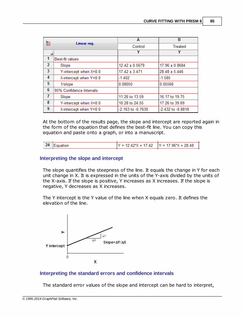
CURVE FITTING WITH PRISM 6 85
© 1995-2014 GraphPad Software, Inc.
At the bottom of the results page, the slope and intercept are reported again inthe form of the equation that defines the best-fit line. You can copy thisequation and paste onto a graph, or into a manuscript.
Interpreting the slope and intercept
The slope quantifies the steepness of the line. It equals the change in Y for eachunit change in X. It is expressed in the units of the Y-axis divided by the units ofthe X-axis. If the slope is positive, Y increases as X increases. If the slope isnegative, Y decreases as X increases.
The Y intercept is the Y value of the line when X equals zero. It defines theelevation of the line.
Interpreting the standard errors and confidence intervals
The standard error values of the slope and intercept can be hard to interpret,

GraphPad Curve Fitting Guide86
© 1995-2014 GraphPad Software, Inc.
but their main purpose is to compute the 95% confidence intervals.
If you accept the assumptions of linear regression , there is a 95% chancethat the 95% confidence interval of the slope contains the true value of theslope, and that the 95% confidence interval for the intercept contains the truevalue of the intercept. The width of the confidence intervals is determined bythe number of data points, their distances from the line, and the spacing of theX values.
Prism can also plot either the confidence or prediction bands .
2.2.2.2 r2, a measure of goodness-of-fit of linear regression
The meaning of r2
The value r2 is a fraction between 0.0 and 1.0, and has no units. An r2 value of0.0 means that knowing X does not help you predict Y. There is no linearrelationship between X and Y, and the best-fit line is a horizontal line goingthrough the mean of all Y values. When r2 equals 1.0, all points lie exactly on astraight line with no scatter. Knowing X lets you predict Y perfectly.
How r2 is computed
This figure demonstrates how Prism computes r2.
The left panel shows the best-fit linear regression line This lines minimizes thesum-of-squares of the vertical distances of the points from the line. Thosevertical distances are also shown on the left panel of the figure. In this example,the sum of squares of those distances (SSreg) equals 0.86. Its units are the
91
171
CURVE FITTING WITH PRISM 6 87
© 1995-2014 GraphPad Software, Inc.
units of the Y-axis squared. To use this value as a measure of goodness-of-fit,you must compare it to something.
The right half of the figure shows the null hypothesis -- a horizontal line throughthe mean of all the Y values. Goodness-of-fit of this model (SStot) is alsocalculated as the sum of squares of the vertical distances of the points from theline, 4.907 in this example. The ratio of the two sum-of-squares valuescompares the regression model with the null hypothesis model. The equation tocompute r2 is shown in the figure. In this example r2 is 0.8428. The regressionmodel fits the data much better than the null hypothesis, so SSreg is muchsmaller than SStot, and r2 is near 1.0. If the regression model were not muchbetter than the null hypothesis, r2 would be near zero.
You can think of r2 as the fraction of the total variance of Y that is "explained"by variation in X. The value of r2 (unlike the regression line itself) would be thesame if X and Y were swapped. So r2 is also the fraction of the variance in Xthat is "explained" by variation in Y. In other words, r2 is the fraction of thevariation that is shared between X and Y.
In this example, 84% of the total variance in Y is "explained" by the linearregression model. The variance (SS) of the data from the linear regressionmodel equals only 16% of the total variance of the Y values (SStot).
Why Prism doesn't report r2 in constrained linear regression
Prism does not report r2 when you force the line through the origin (or anyother point), because the calculations would be ambiguous. There are twoways to compute r2 when the regression line is constrained. As you saw in theprevious section, r2 is computed by comparing the sum-of-squares from theregression line with the sum-of-squares from a model defined by the nullhypothesis. With constrained regression, there are two possible nullhypotheses. One is a horizontal line through the mean of all Y values. But thisline doesn't follow the constraint -- it does not go through the origin. The othernull hypothesis would be a horizontal line through the origin, far from most ofthe data.
Because r2 is ambiguous in constrained linear regression, Prism doesn't reportit. If you really want to know a value for r2, use nonlinear regression to fit yourdata to the equation Y=slope*X. Prism will report r2 defined the first way(comparing regression sum-of-squares to the sum-of-squares from ahorizontal line at the mean Y value).
Upper or lower case?
With linear regression, it is conventional to use the abbreviation r2. With

GraphPad Curve Fitting Guide88
© 1995-2014 GraphPad Software, Inc.
nonlinear regression, the convention is to use R2. There appears to be noreason for this distinction.
2.2.2.3 Is the slope significantly different than zero?
Interpreting the P value when Prism fits both slope and intercept
Prism reports the P value testing the null hypothesis that the overall slope iszero. The P value answers this question:
If there were no linear relationship between X and Y overall, what is theprobability that randomly selected points would result in a regression line asfar from horizontal (or further) than you observed?
Equivalently:
If there were no linear relationship between X and Y overall, what is theprobability that randomly selected points would result in an R2 value as high(or further) as you observed?
The P value is calculated from an F test, and Prism also reports the value of Fand its degrees of freedom. You would get exactly the same P value from the tratio computed by dividing the slope by its standard error.
Interpreting the P value when Prism fits only the slope
Beware of the P value from linear regression when you force the line to gothrough the origin or some other point. It is easy to misinterpret. The graphbelow demonstrates the problem:
The data points almost form a horizontal line.
When fit with linear regression the usual way (fit both slope and intercept;
CURVE FITTING WITH PRISM 6 89
© 1995-2014 GraphPad Software, Inc.
green line), the best fit value of the slope is 0.00. The P value answers thequestion: If the true slope is zero, what is the chance that the slope will befurther from zero than the observed slope due only to random sampling. Sincethe observed slope is zero, there is almost a 100% chance of obtaining a slopethat is further than zero than observed! So the P value is greater than 0.99, ashigh as a P value can be. Some people are confused and think the P valueshould be small purely because the points for a pattern. Not so. The P value,from conventional linear regression fitting both slope and intercept, will be smallonly when the points form a linear pattern that is not horizontal.
The results are very different when you fit linear regression with the constraintthat the line has to go through the origin (blue line). To make the line gothrough the origin and also go near the points, the best-fit line has a slope is farfrom zero. Since the line is far from horizontal, the P value is tiny. Given theconstraint that the line must go through the origin (X=0, Y=0; lower-left ofgraph), the data are quite convincing that best fit line is far from horizontal, soit makes sense that the P value is tiny.
Constraining a line to go through the origin (or some other point) can be veryuseful in some situations. Usually this option is used to fit calibration curvesused for interpolation, in which case the P value is not useful. If you force theline through the origin, be very wary when interpreting the P value. It is rarelyuseful, and easy to misinterpret.
Download the Prism file.
2.2.2.4 Comparing slopes and intercepts
Prism compares slopes of two or more regression lines if you check the option: "Test whether the slopes and intercepts are significantly different".
Comparing slopes
Prism compares slopes first. It calculates a P value (two-tailed) testing the nullhypothesis that the slopes are all identical (the lines are parallel). The P valueanswers this question:
If the slopes really were identical, what is the chance that randomly selecteddata points would have slopes as different (or more different) than youobserved.

GraphPad Curve Fitting Guide90
© 1995-2014 GraphPad Software, Inc.
If the P value is less than 0.05
If the P value is low, Prism concludes that the lines are significantly different. Inthat case, there is no point in comparing the intercepts. The intersection pointof two lines is:
If the P value for comparing slopes is greater than 0.05
If the P value is high, Prism concludes that the slopes are not significantlydifferent and calculates a single slope for all the lines. Essentially, it shares theSlope parameter between the two data sets.
Comparing intercepts
If the slopes are significantly different, there is no point comparing intercepts. Ifthe slopes are indistinguishable, the lines could be parallel with distinctintercepts. Or the lines could be identical. with the same slopes and intercepts.
Prism calculates a second P value testing the null hypothesis that the lines areidentical. If this P value is low, conclude that the lines are not identical (they aredistinct but parallel). If this second P value is high, there is no compellingevidence that the lines are different.
Relationship to ANCOVA and global regression
This method is equivalent to an Analysis of Covariance (ANCOVA), althoughANCOVA can be extended to more complicated situations. It also is equivalentto using Prism's nonlinear regression analysis with a straight-line model, andusing an F test to compare a global model where slope is shared among thedata sets with a model where each dataset gets its own slope.
Reference
Chapter 18 of J Zar, Biostatistical Analysis, 2nd edition, Prentice-Hall, 1984.
2.2.2.5 Runs test following linear regression
The runs test determines whether your data differ significantly from a straight
41

CURVE FITTING WITH PRISM 6 91
© 1995-2014 GraphPad Software, Inc.
line. Prism can only calculate the runs test if you entered the X values in order.
A run is a series of consecutive points that are either all above or all below theregression line. In other words, a run is a consecutive series of points whoseresiduals are either all positive or all negative.
If the data points are randomly distributed above and below the regression line,it is possible to calculate the expected number of runs. If there are Na pointsabove the curve and Nb points below the curve, the number of runs you expectto see equals [(2NaNb)/(Na+Nb)]+1. If you observe fewer runs than expected,it may be a coincidence of random sampling or it may mean that your datadeviate systematically from a straight line. The P value from the runs testanswers this question:
If the data really follow a straight line, and you performed many experimentslike this one, what fraction of the time would you obtain as few (or fewer)runs as observed in this experiment?
If the runs test reports a low P value, conclude that the data do not reallyfollow a straight line, and consider using nonlinear regression to fit a curve.
The P values are always one-tail, asking about the probability of observing asfew runs (or fewer) than observed. If you observe more runs than expected,the P value will be higher than 0.50.
.
2.2.2.6 Analysis checklist: Linear regression
Can the relationship between X and Y be graphed as a straight line?
In many experiments the relationship between X and Y is curved, making linearregression inappropriate. It rarely helps to transform the data to force the relationshipto be linear. Better, use nonlinear curve fitting.
Is the scatter of data around the line Gaussian (at least approximately)?
Linear regression analysis assumes that the scatter of data around the best-fit line isGaussian.
Is the variability the same everywhere?
Linear regression assumes that scatter of points around the best-fit line has the samestandard deviation all along the curve. The assumption is violated if the points with

GraphPad Curve Fitting Guide92
© 1995-2014 GraphPad Software, Inc.
high or low X values tend to be further from the best-fit line. The assumption that thestandard deviation is the same everywhere is termed homoscedasticity. (If the scattergoes up as Y goes up, you need to perform a weighted regression. Prism can't do thisvia the linear regression analysis. Instead, use nonlinear regression but choose to fit toa straight-line model.
Do you know the X values precisely?
The linear regression model assumes that X values are exactly correct, and thatexperimental error or biological variability only affects the Y values. This is rarely thecase, but it is sufficient to assume that any imprecision in measuring X is very smallcompared to the variability in Y.
Are the data points independent?
Whether one point is above or below the line is a matter of chance, and does notinfluence whether another point is above or below the line.
Are the X and Y values intertwined?
If the value of X is used to calculate Y (or the value of Y is used to calculate X) thenlinear regression calculations are invalid. One example is a Scatchard plot, where the Yvalue (bound/free) is calculated from the X value. Another example would be a graphof midterm exam scores (X) vs. total course grades(Y). Since the midterm exam scoreis a component of the total course grade, linear regression is not valid for these data.
2.2.2.7 Graphing tips: Linear regression
Graphing the regression line
When Prism performs linear regression, it automatically superimposes the lineon the graph.
If you need to create additional graphs, or change which line is plotted on whichgraph, keep in mind that the line generated by linear regression is seen by Prismas a data set. You can add lines to a graph or remove lines from a graph on the'Data sets on graph' tab of the Format Graph dialog.
Confidence and prediction bands
If you check the option box, Prism will calculate and graph either the 95%confidence band or 95% prediction band of the regression line.

CURVE FITTING WITH PRISM 6 93
© 1995-2014 GraphPad Software, Inc.
Confidence bands
Two confidence bands surrounding the best-fit line define the confidence intervalof the best-fit line.
The dashed confidence bands are curved. This does not mean that theconfidence band includes the possibility of curves as well as straight lines.Rather, the curved lines are the boundaries of all possible straight lines. Thefigure below shows four possible linear regression lines (solid) that lie within theconfidence band (dashed).
Given the assumptions of linear regression, you can be 95% confident that thetwo curved confidence bands enclose the true best-fit linear regression line,leaving a 5% chance that the true line is outside those boundaries.
Many data points will be outside the 95% confidence bands. The confidencebands are 95% sure to contain the best-fit regression line. This is not the sameas saying it will contain 95% of the data points.
Prediction bands
Prism can also plot the 95% prediction bands. The prediction bands are furtherfrom the best-fit line than the confidence bands, a lot further if you have manydata points. The 95% prediction band is the area in which you expect 95% of alldata points to fall. In contrast, the 95% confidence band is the area that has a

GraphPad Curve Fitting Guide94
© 1995-2014 GraphPad Software, Inc.
95% chance of containing the true regression line. This graph shows bothprediction and confidence intervals (the curves defining the prediction intervalsare further from the regression line).
When to plot confidence and prediction bands
The confidence bands sort of combine the confidence intervals of the slope andintercept in a visual way. Use confidence bands to learn how precisely your datadefine the best-fit line.
Prediction bands are wider, to also include the scatter of the data. Useprediction bands when your main goal is show the variation in your data.
Fine-tuning the appearance of the confidence and prediction bands
If you check the option on the Linear regression, Prism will automaticallysuperimpose the confidence or prediction band on the graph.
To adjust the appearance of the confidence or prediction bands, go to theFormat Graph dialog, select the dataset that represents the best fit curve, andadjust the error bars and area fill settings. You can also choose to fill the areaenclosed by the confidence or prediction bands.

CURVE FITTING WITH PRISM 6 95
© 1995-2014 GraphPad Software, Inc.
Residuals
If you check an option on the linear regression dialog, Prism will create a resultstable with residuals, which are the vertical distances of each point from theregression line. The X values in the residual table are identical to the X valuesyou entered. The Y values are the residuals. A residual with a positive valuemeans that the point is above the line; a residual with a negative value meansthe point is below the line.
When Prism creates the table of residuals, it also automatically makes a newgraph containing the residuals and nothing else. You can treat the residuals tablelike any other table, and do additional analyses or make additional graphs.
If the assumptions of linear regression have been met, the residuals will berandomly scattered above and below the line at Y=0. The scatter should notvary with X. You also should not see large clusters of adjacent points that areall above or all below the Y=0 line.
See an example of residuals from nonlinear regression.
2.2.2.8 Questions and answers
What is the difference between correlation and linear regression?
The answer is in the Correlation section.
Why is the 95% confidence interval of the X intercept asymmetrical?
The 95% confidence interval for the X-intercept is not symmetrical aroundthe X-intercept. It goes further in one direction than the other, as illustratedin the graph below.
179
16

GraphPad Curve Fitting Guide96
© 1995-2014 GraphPad Software, Inc.
Follow the Y=0 baseline from left to right. The region between the 95%confidence bands for the best fit line (blue curves) is the 95% CI of the Xintercept. You can see that this confidence interval (between the twooutmost dotted lines) is not symmetrical around the X intercept (the middledotted line).
This asymmetry will be very noticeable if you only have a few points with lotsof scatter, and will be almost unnoticeable with lots of points with littlescatter.
GraphPad Prism reports the 95% confidence interval of the X intercept if youcheck an option on the Linear regression parameters dialog.
Because the uncertainty is not symmetrical, it rarely makes sense to report astandard error of the X-intercept. It is much better to report both ends of the95% confidence interval, which Prism reports. If you really want to computea single standard error for the X intercept, you can do so by choosingnonlinear regression, and fitting this user-defined equation to the data:
Y = slope*(X-Xintercept)
Prism will report the best-fit value of the X intercept along with a SE and 95%confidence interval. Since this confidence interval will be computed from theSE value it will be symmetrical around the X intercept, and so won't be asaccurate as the asymmetrical interval reported by linear regression.

CURVE FITTING WITH PRISM 6 97
© 1995-2014 GraphPad Software, Inc.
How to test whether the slope from linear regression differs from 1.0 or some other value?
Prism tests whether the best-fit slope from linear regression line differssignificantly from zero. But you need to use extra steps to test whether theslope differs from some other value.
Since Prism's linear regression analysis can't answer the question, usenonlinear regression instead. Nonlinear regression can fit a straight line and offers many advantages .
In the nonlinear regression parameters dialog, go to the Compare tab, checkthe option to ask compare the best-fit value of a parameter to a theoreticalvalue, and then choose Slope and enter the theoretical value (1.0).
Can Prism do weighted linear regression?
Prism's linear regression analysis cannot handle differential weighting.However, Prism's nonlinear regression analysis can do weighted regression,and you can fit a straight line using "nonlinear" regression .
How can Prism fit linear regression with the slope constrained to equal 1.0 (or some othervalue)?
Prism's linear regression analysis cannot constrain the slope to a particularvalue. However, Prism's nonlinear regression analysis can constrain anyparameter to any value, and you can fit a straight line using "nonlinear"regression .
How to fit one linear regression line to multiple data sets?
Prism usually fits one line through each data set. But you can get it to fit oneline through all the data. Use the nonlinear regression analysis to fit the line. Then go to the Constrain tab, and share both the slope and the intercept."Sharing" means that Prism fits one best-fit value for all the data sets, ratherthan one for each data set. Since you share all the parameters, only one lineis fit to all the data.
Why doesn't Prism report R2 for linear regression when I force the line through the origin(or some other point)?
The problem is that when you constrain a line to go through a point, therewould be two ways to compute R2:
Compare the fit of the best-fit line with the fit of a horizontal line at the
mean Y value. But that null hypothesis (horizontal line through the Ymean)
82
82
82
82

GraphPad Curve Fitting Guide98
© 1995-2014 GraphPad Software, Inc.
doesn't obey the constraint that it go through the origin.
Compare the best-fit line with a horizontal line at Y=0. This obeys the
constraint, but often fits the data really badly, pushing up the R2 value.
Since R2 is ambiguous when you constrain linear regression, Prism simplydoes not report it when you force the line through the origin (or otherpoint).
If you fit the line with nonlinear regression, Prism will report R2 using the firstdefinition above.
Fitting the crossing point of two intersecting linear regression lines .
Enter your data onto one data table, with Y values in columns A and B nextto corresponding X values in the X column. If the X values don't match forthe two data sets, just leave some Y values blank.
Use nonlinear regression, and enter this user-defined equation.
Y= Ycross + (X - Xcross)*Slope
This equation defines the Y coordinate of any point along either line to equalthe Y coordinate of the crossing point plus the slope times the X distancefrom the crossing point to that point.
Set these rules for initial values:
Ycross: 1*Ymid (the average of the highest and lowest Y values)
Xcross: 1*Xmid
Slope: 1*(Ymax-Ymin)/(Xmax-Xmin).
Define Xcross and Ycross to both be shared parameters, so Prism will findone global best-fit value for those parameters that applies to both data sets.Do not share the slope parameter, as you want Prism to fit separate slopesfor each data set. Getting these sharing settings correct is essential.
Prism will fit four parameters:
Slope for the first data set
Slope for the second data set

CURVE FITTING WITH PRISM 6 99
© 1995-2014 GraphPad Software, Inc.
Xcross (shared for both data sets)
Ycross (shared for both data sets).
That makes sense. You have two lines, and it takes two parameters (usuallya slope and intercept) to describe each. Here, the equations were rearrangedso the program doesn't fit two separate Y intercepts, but rather fits the Xand Y values of the crossing point.
Here is an example, with the key results circled. Prism file.

GraphPad Curve Fitting Guide100
© 1995-2014 GraphPad Software, Inc.
2.2.3 Deming regression
2.2.3.1 Key concepts: Deming regression
Standard linear regression assumes that you know the X values perfectly,and all the uncertainty is in Y. It minimizes the sum of squares of the verticaldistance of the points from the line.
If both X and Y variables are subject to error, fit linear regression using amethod known as Deming, or Model II, regression.
If your goal is to compare two analysis methods, consider using a Bland-Altmanplot instead.
2.2.3.2 How to: Deming regression
1. Create a data table
From the Welcome or New Table dialog, choose to create XY data table.
If you are just getting started, choose the sample data: Linear regression --Compare slopes.
If you are entering your own data, choose a to enter a single Y value for eachpoint (no replicates, no error values).
2. Enter data
If you enter Y values for several data sets (column A, B and C), Prism willreport regression results for X vs. YA, for X vs. YB, and for X vs. YC.
3. Analysis choices
Click Analyze and choose Deming regression from the list of XY analyses.
Most of the dialog is self-explanatory. The choices on top are the hardest tounderstand, but also are the most important as the calculations depend onknowing relative magnitude of the errors in X and Y.
13

CURVE FITTING WITH PRISM 6 101
© 1995-2014 GraphPad Software, Inc.
X and Y have equal uncertainty
If you are comparing two analytical methods, X and Y, assessed in the sameunits, you will probably find it reasonable to assume that both share the samestandard deviation. In this case, check the first option. There is no need toestimate that standard deviation. It is enough to declare that X and Y haveequal standard deviations. In this case, Deming regression minimizes the sumof the squares of the perpendicular distances of the points from the line. This isalso called orthogonal regression.
X and Y have different uncertainties
If you are not willing to assume that X and Y have the same amount ofuncertainty, then you need to enter the SD of each. Enter the SD of X values inthe same units as X values are entered, and the SD of Y values in the sameunits as Y values are entered. Don't enter the SD of all X (or Y) values youenter. Enter the average SD (determined separately) of repeatedmeasurements of X and Y.
How do you know what values to enter? To assess the uncertainty (error) of amethod, collect duplicate measurements from a number of samples using thatmethod. Calculate the standard deviation of the error using the equationbelow(1), where each d
i is the difference between two measurements of the
same sample (or subject), and N is the number of measurements you made (Nequals twice the number of samples, since each sample is measured twice).
2i
error
dSD =
N
Compute the SD of the error for each method or variable (X and Y), enter thetwo SD
error values into the Deming regression analysis dialog, and Prism will fit
the line for you. If the X variable has a much smaller SD than the Y value, theresults will be almost identical to standard linear regression.
If you try to compare Prism’s results with those of another program or book,

GraphPad Curve Fitting Guide102
© 1995-2014 GraphPad Software, Inc.
you may encounter the variable (lambda), which quantifies the inequality
between X and Y errors.
2
X error
Y error
SDλ=
SD
Prism requires you to enter individual SD values, but uses these values only tocalculate , which is then used in the Deming regression calculations. If you
know , but not the individual SD values, enter the square root of as the SD
of the X values, and enter 1.0 as the SD of the Y error. The calculations will becorrect, since Prism uses those two values only to compute .
Reference
1. PW Strike, Statistical Methods in Laboratory Medicine, ISBN:0750613459. Equation8.15.
2.2.3.3 Q&A: Deming Regression
Why doesn't Prism report R2 with Deming Regression results?
When Prism performs Deming regression, it reports the slope and interceptswith confidence intervals, and reports a P value testing the null hypothesis thatthe slope is really zero. However, Prism does not report any measure ofgoodness-of-fit with Deming regression, and so does not report R2. The reasonis that we have been unable to find any paper or text that would explain how tocompute or interpret such a value. In ordinary linear or nonlinear regression, R2
is the fraction of the variation that is accounted for by the model. But withDeming regression, this definition doesn't really make sense, and it isn't obviousto us how to extend it.
Is Deming regression the same as orthogonal linear regression?
In Prism's Deming dialog, you specify whether X and Y are in the same unitswith equal uncertainties (variation). If you choose this option, Demingregression minimizes the sum of the square of the perpendicular distances ofthe points from the line. This is also called orthogonal linear regression. If youspecify different SD values for X and Y, then Deming regression is not the sameas orthogonal linear regression.
How was the equation to compute the SD from a set of duplicatemeasurements derived?
The previous page showed the equation for assessing the uncertainty (error) ofa method from duplicate measurements from a number of samples using that

CURVE FITTING WITH PRISM 6 103
© 1995-2014 GraphPad Software, Inc.
method:
2i
error
dSD =
N
It is easy to derive that equation. To compute the variance, you find theaverage square of the difference between each value and the mean. For pairs,the mean is half the difference. So take half that distance squared, but alsocompute it for the other value of the pair. For both values, therefore, thecontribution is d
i squared. Add that up for all the measurements and divide by
the number of measurements, and you have the variance. Take the squareroot to get the SD.
Why N, rather than N-1? I suspect it should be N-1, but that won't mattermuch. It will make the SD a bit smaller than it should be, but that will be true forboth the X and Y SD, so the ratio will hardly be changed.
2.2.3.4 Analysis checklist: Deming regression
Can the relationship between X and Y be graphed as a straight line?
In many experiments the relationship between X and Y is curved, making linearregression inappropriate. It rarely helps to transform the data to force the relationshipto be linear. Better, use nonlinear curve fitting.
Are the data points independent?
Whether one point is above or below the line is a matter of chance, and does notinfluence whether another point is above or below the line.
Are the X and Y values intertwined?
If the value of X is used to calculate Y (or the value of Y is used to calculate X) thenlinear regression calculations are invalid. One example is a Scatchard plot, where the Yvalue (bound/free) is calculated in part from the X value (bound). Another examplewould be a graph of midterm exam scores (X) vs. total course grades(Y), since Y is inpart computed from X.
Do you know the relative uncertainty of X and Y?
Ordinary linear regression assumes that you know the X values perfectly, and all theuncertainty is in Y. Deming regression assumes there is uncertainty in both variables.You have to specify the relative uncertainties, either by specifying that X and Y areequally uncertain or by entering the SD of each. If these values are incorrect, the

GraphPad Curve Fitting Guide104
© 1995-2014 GraphPad Software, Inc.
Deming results won't be useful.
2.3 Interpolating from a standard curve
Prism makes it very easy to interpolate unknown values from astandard curve. Enter the standards with both X and Y values,fit a line or curve, and Prism will tell you which X valuescorrespond to Y values you entered on the same data table.
Key concept: Interpolating
How to interpolate
Equations used for interpolating
Where are the interpolated results?
When X values are logarithms
Analysis checklist: Interpolating
Q&A: Interpolating
Standard Addition Method
2.3.1 Key concept: Interpolating
A common use of nonlinear (and linear) regression is interpolating.The basicidea is simple:
1.Enter a standard curve. Each point consists of a concentration (or logarithmof concentration) and a response. The responses are commonly radioactivity,fluorescence, or optical density.
2.Fit a line or curve through the standards. For this purpose, you don't muchcare about the meaning of the model, or the interpretation of the best-fitvalues of the parameters (EC50, etc.).
3.For unknown samples, you know the response, but not the concentration.So read the concentration from the curve:
104
105
111
113
117
118
121
123

CURVE FITTING WITH PRISM 6 105
© 1995-2014 GraphPad Software, Inc.
Notes:
This graph shows the response going up as the concentration gets larger. In
many cases, the response goes down as the concentration gets larger.Interpolation works in either case.
Sigmoid shaped dose-response curves are commonly used with many
assays. If the X values analyzed by the analysis are the logarithm ofconcentration, then so are the interpolated values. You need to take the antilogarithm of these values to return to concentration units.
This example shows the most common use of interpolating. Finding an X
value (concentration) for a given Y value. Prism can also interpolate the otherway: Finding a Y value for an entered X value.
2.3.2 How to interpolate
Prism is not designed to analyze any particular kind of assay
Prism is a very general program, used by scientists in many fields. It is easy foryou to interpolate standard curves using Prism, but you must make somedecisions. Unlike some specialized programs, Prism is not set up so you canblindly enter data and get results without thinking.
Entering data for interpolation
Enter the standard curve in the top rows of a table, and then enter the

GraphPad Curve Fitting Guide106
© 1995-2014 GraphPad Software, Inc.
unknown values right below those standards. In most cases, as shown below,you'll enter Y values and leave X blank. Prism can also interpolate the otherway. In this case, enter X values and leave Y blank.
Entering labels for the unknowns, as shown below, is optional.
Note that it is essential that the unknowns go below the standard curve values.If you place the unknowns above the standard curve, Prism will not interpolate.Of course, the unknown Y values must be in the same units as the Y values youentered for the standard curve.
Fitting a standard curve and interpolating
Four analyses in Prism let you interpolate values from curves. The top row ofbuttons in the analysis block provide shortcuts to linear regression, nonlinlearregression, and the simplified analysis for interpolating a standard curve.
Interpolate a standard curve
This analysis (new to Prism 6) is a simple way to interpolate using nonlinearregression.
The choices on the dialog are simple. Choose a model to fit to your data. The mostcommonly used models for standard curves are shown in the dialog. Next choose howto handle outliers. You can choose to use robust regression , so outliers have littleimpact. Or you can ask Prism to identify, and perhaps eliminate, outliers using the ROUT
111
59

CURVE FITTING WITH PRISM 6 107
© 1995-2014 GraphPad Software, Inc.
method . Finally, if the scatter among replicates is larger when the Y values are larger,consider using relative weighting .
Note that this simplified analysis to interpolate is simply a subset of thenonlinear regression analysis, with fewer choices on the dialog. If you want toselect options that aren't available, click the "More.." button at the bottom ofthe dialog to convert the analysis to the full nonlinear regression analysis, withmany more options (six tabs worth). Once you switch to nonlinear regressionanalysis, it is not possible to switch back (except by starting over).
Nonlinear regression
Nonlinear regression offers the interpolation option at the bottom of the first(Fit) tab of the dialog. This is a good choice if you want to use options notavailable on the simpler interpolation analysis.
Linear regression
Linear regression offers a checkbox to interpolate the top of the dialog.
Spline
Prism can also interpolate from a standard curve in the spline analysis. Splines gothrough every point. The advantage of a spline is that you don't have to choose a model tofit to your data. The disadvantage is that the curve may wiggle too much.
2.3.3 Example: Interpolating from a sigmoidal standard curve
1. Create the data table
From the Welcome or New Table dialog, choose to create an XY data table, andselect the sample data set: RIA or ELISA. Interpolate unknowns from sigmoidalcurve.
2. Inspect the data
The sample data may be partly covered by a floating note explaining how to fitthe data (for people who are not reading this help page). You can move thefloating note out of the way, or minimize it.
57
160
79
447

GraphPad Curve Fitting Guide108
© 1995-2014 GraphPad Software, Inc.
The first seven rows contain the standard curve, in duplicate. Below that arethree unknown values. These have a Y values that you measured, but no X.The goal of this analysis is to interpolate the corresponding X values(concentrations) for these unknowns. Note that three of the four unknownsare labeled, so you can later match up the results with the labels.
Why are X values negative? Because in this example, the X values are thelogarithm of concentrations expressed in molar. So a concentration of 1micromolar (10-6 Molar) would be entered as -6.
3. View the graph
The graph Prism makes automatically is fairly complete. You can customize thesymbols, colors, axis labels, etc. You can also choose to plot the individualduplicates rather than plot the means. Since the unknowns have no X value,they are not included on the graph.

CURVE FITTING WITH PRISM 6 109
© 1995-2014 GraphPad Software, Inc.
4. Choose the standard curve analysis
Click and from the list of XY analyses choose: Interpolate aStandard Curve.
Alternatively, you can click the “Interpolate a standard curve” button right ontop of the Analyze button.
5. Choose a model
Choose the equation: Sigmoidal, 4PL, X is log(Concentration). Note that 4PLmeans four parameter logistic, which is another name for this kind of equation.
For this example, leave all the other settings to their default values.
Click OK to see the curves superimposed on the graph.

GraphPad Curve Fitting Guide110
© 1995-2014 GraphPad Software, Inc.
6. Inspect the results
The results appear on several pages.
The first page shows you the interpolated values.
The second page is the table of results for the overall curve fit. It tabulates thebest-fit values of the parameters and much more. For this example, we aren'ttoo interested in these results.
7. Transform the results
The X column of the results table has the interpolated values we want. Theseare in the same units as the X values, so are the logarithm of concentration.Prism can transform these values to concentration units.
Click and choose Transform at the top of the Analyze dialog.
On the Transform dialog check the option to transform X values and choosethe transform X=10^X

CURVE FITTING WITH PRISM 6 111
© 1995-2014 GraphPad Software, Inc.
Now the X column is in molar concentration units. Note that the column titlehasn't changed. Prism isn't smart enough to adjust the column titles when youtransform data.
Click and edit the column title to "Concentration (M)".
2.3.4 Equations used for interpolating
You can interpolate from any curve fit through a set of standards. However, theequations listed below are used most commonly. These equations are instantlyavailable from the interpolation analysis. You'll also find this set of equations inthe equation tree used in nonlinear regression.
Notes:
These graphs show the curve going up (increasing Y) as X increases. But all
will work for downward sloping curves too.
All of these equations are also present in other equation folders in the
nonlinear regression dialog.
Sigmoidal, 4PL, Xislog(concentration) 256

GraphPad Curve Fitting Guide112
© 1995-2014 GraphPad Software, Inc.
AsymmetricSigmoidal, 5PL, Xislog(concentration)
Biphasic
Straight line
Semilog line -- Xis log, Y is linear
267
269
371
376

CURVE FITTING WITH PRISM 6 113
© 1995-2014 GraphPad Software, Inc.
Hyperbola (X isconcentration)
Second orderpolynomial(quadratic)
Y=B0 + B1*X + B2*X^2
Third orderpolynomial (cubic)
Y=B0 + B1*X + B2*X^2 + B3*X^3
2.3.5 The results of interpolation
Where are the interpolated results?
Prism places the interpolation results into its an additional results page (or twoadditional pages).
To view this table, click the interpolated results page of the results. In somecases you may first need to click the + in front of the results main page to seeall the pages within.
297
384
384

GraphPad Curve Fitting Guide114
© 1995-2014 GraphPad Software, Inc.
What units are the results in?
The interpolated results are expressed in the same units as the standardcurves. If you entered a Y value, and Prism interpolated an X value, then that Xvalue is in the same units as the standards you entered.
If the X values in the table are the logarithm of concentration (common), thenthe interpolated results are also logarithms of concentration.
In some assays, different samples are diluted differently. Prism does not correctfor dilution, so you'll need to make those corrections manually.
2.3.6 Interpolating with replicates in side-by-side subcolumns
Choices when entering data with replicates in subcolumns
It is common to enter replicate values for the unknowns, as shown below.

CURVE FITTING WITH PRISM 6 115
© 1995-2014 GraphPad Software, Inc.
Since Prism's results tables cannot be configured to put side-by-side replicates inthe X column, you have two choices for how to organize the results. Thesechoices are available at the bottom of the Output tab of the nonlinear regressiondialog.
Place computed unknown values into the X column, with replicate valuesstacked
In this case, Prism creates two pages of results.
The interpolation is the same for both tables. Prism interpolates each replicatevalue individually.
The first page, Interpolated Mean X Values, shows the mean of the Y valuesyou entered and the mean of the interpolated X values. The X column showsthe concentrations (or logarithm of concentrations) to match the data youentered.
The second page, Interpolated X replicates, shows individual replicate values forthe interpolated results. The X column maintains the same meaning as it does inthe data table you entered. To do so, with only a single X column, requires thatthe replicates be stacked.
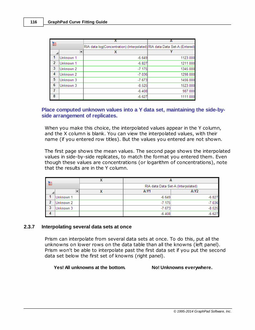
GraphPad Curve Fitting Guide116
© 1995-2014 GraphPad Software, Inc.
Place computed unknown values into a Y data set, maintaining the side-by-side arrangement of replicates.
When you make this choice, the interpolated values appear in the Y column,and the X column is blank. You can view the interpolated values, with theirname (if you entered row titles). But the values you entered are not shown.
The first page shows the mean values. The second page shows the interpolatedvalues in side-by-side replicates, to match the format you entered them. Eventhough these values are concentrations (or logarithm of concentrations), notethat the results are in the Y column.
2.3.7 Interpolating several data sets at once
Prism can interpolate from several data sets at once. To do this, put all theunknowns on lower rows on the data table than all the knowns (left panel).Prism won't be able to interpolate past the first data set if you put the seconddata set below the first set of knowns (right panel).
Yes! All unknowns at the bottom. No! Unknowns everywhere.

CURVE FITTING WITH PRISM 6 117
© 1995-2014 GraphPad Software, Inc.
Why can't Prism handle the kind of data shown in the right panel above?Because then it might get mixed up about which values are unknowns to beinterpolated, and which are simply adjacent to values left blank because theyare missing.
2.3.8 When X values are logarithms
In many situations, you'll fit the standard curve to a log(dose) vs. responsecurve. In these cases, you'll enter the X values for the standard curve as thelogarithm of concentration or you'll transform the data to logarithms beforerunning nonlinear regression.
The interpolated X values are in the same units as the X values the analysissees. If you are analyzing data entered or transformed so X is the logarithm ofconcentration, then the interpolated values will also be logarithms.

GraphPad Curve Fitting Guide118
© 1995-2014 GraphPad Software, Inc.
If you want to transform these results back to concentrations, that is easy todo:
1.From the interpolated results page of results, click Analyze.
2.Choose Transform at the very top of the Analyze dialog.
3.Choose the standard list of transforms.
4.Depending on whether your interpolated values are in the X or Y column,choose to transform that column.
5.From the list of transforms, choose Y=10^Y or X=10^X. These choices areabout one third of the way down the long list of transforms.
6.The results sheets will have the interpolated values as concentrations, ratherthan logs.
Why 10^Y or 10^X? Those are abbreviations for 10Y or 10X , which are theantilogarithm functions. Review logarithms and antilogarithms.
2.3.9 Analysis checklist: Interpolating
Your approach in evaluating nonlinear regression depends on your goal.
In many cases, your goal is to learn from the best-fit values. If that is yourgoal, view a different checklist .
If your goal is to create a standard curve from which to interpolate unknownvalues, your approach depends on whether this is a new or established assay.
Established assay
If the assay is well established, then you know you are fitting the right modeland know what kind of results to expect. In this case, evaluating a fit is prettyeasy.
Does the curve go near the points?
Is the R2 'too low' compared to prior runs of this assay?
If so, look for outliers, or use Prism's automatic outlier detection.
113
218

CURVE FITTING WITH PRISM 6 119
© 1995-2014 GraphPad Software, Inc.
Are the confidence bands too wide?
The confidence bands let you see how accurate interpolations will be, so wesuggest always plotting prediction bands when your goal is to interpolate fromthe curve. If your are running an established assay, you know how wide youexpect the prediction bands to be.
New assay
With a new assay, you also have to wonder about whether you picked anappropriate model.
Does the curve go near the points?
Look at the graph. Does it look like the curve goes near the points.
Are the confidence bands too wide?
How wide is too wide? The prediction bands show you how preciseinterpolations will be. Draw a horizontal line somewhere along the curve, andlook at the two places where that line intercepts the confidence bands. This willbe the confidence interval for the interpolation.
Does the scatter of points around the best-fit curve follow a Gaussiandistribution?
Least squares regression is based on the assumption that the scatter of pointsaround the curve follows a Gaussian distribution. Prism offers three normalitytests (in the Diagnostics tab) that can test this assumption (we recommend theD'Agostino test). If the P value for a normality test is low, you conclude thatthe scatter is not Gaussian.
Could outliers be impacting your results?
Nonlinear regression is based on the assumption that the scatter of dataaround the ideal curve follows a Gaussian distribution. This assumption leads tothe goal of minimizing the sum of squares of distances of the curve from thepoints. The presence of one or a few outliers (points much further from thecurve than the rest) can overwhelm the least-squares calculations and lead tomisleading results.
You can spot outliers by examining a graph (so long as you plot individualreplicates, and not mean and error bar). But outliers can also be detected
171

GraphPad Curve Fitting Guide120
© 1995-2014 GraphPad Software, Inc.
automatically. GraphPad has developed a new method for identifying outlierswe call the ROUT method. You can either ask Prism to simply identify outliers orto eliminate them. These choices are adjacent on the Interpolate a StandardCurve dialog. But they are in separate tabs in the Nonlinear Regression dialog.The option to count outliers is on the Diagnostics tab, and the the option toexclude outliers is on the Fit tab.
Does the curve deviate systematically from the data?
If either the runs test or the replicates test yields a low P value, then you canconclude that the curve doesn't really describe the data very well. You mayhave picked the wrong model.
2.3.10 Reasons for blank (missing) results
Interpolated value is blank
When you ask Prism to interpolate X values from Y values you enter, it willleave the result blank when it is unable to find a result. This can happen when:
The input value for Y falls out of the vertical range of the standard curve. This
happens when you fit a sigmoidal log(dose) vs response curve. If you enteran unpaired Y value that is larger than the best-fit value of Top, or smallerthan the best-fit value of Bottom, there simply is no corresponding X value,and Prism will simply leave that part of the Results sheet blank. Note that"top" and "bottom" apply to the best-fit values for those fitted parameters,not the maximum and minimum values of the input data. It simply isimpossible to interpolate a X value if the Y value is too high, or too low, to beon the curve.
The interpolated X value falls way outside the output range of X for the fitted
curve. Prism will try to extrapolate a bit beyond the range of X values forwhich it calculates and draws the curve. But it won't extrapolate far from theends of the curve. You can extend this range. From the Nonlinear regressionParameters dialog, choose the Range tab and enter a lower value for theminimum X and/or a higher value for the maximum X.
You entered the unknowns in rows above the standard curve values. The
unknowns must be entered in rows below the standards.
You mistakenly entered the unknowns in the wrong units. The unknown
values must be in the same units as the standards. If you enter unknown Y

CURVE FITTING WITH PRISM 6 121
© 1995-2014 GraphPad Software, Inc.
values and expect Prism to interpolate an X value, then the unknown Y valuesmust be entered in the same units as the Y values for the standards.
Confidence interval of interpolated value is blank
Prism can also report the 95% confidence interval for the interpolated values. Itonly does this when the interpolated X value is within the range of the standardcurve. If the interpolated value is extrapolated beyond that range, Prism leavesthe confidence interval blank.
2.3.11 Q&A: Interpolating
Expand all
Collapse all
Can Prism interpolate several data sets at once?
Yes, Prism can interpolate X values from Y values entered into several datasets. Note the following:
Prism has to figure out which values are unknowns. It uses this rule: X(or
Y) values are considered as unpaired (and are used for calculation ofunknowns) when they are lower in the table than all XY pairs in the datatable. It is not enough that the unpaired Y values (from which you wantPrism to interpolate X) is lower on the table than the paired XY values forthat particular data set. They must be on lower rows in the table than allthe paired XY values of all data sets in the table.
Prism offers an option in the Output tab of nonlinear regression that let
you choose where the interpolated X values should go (into the X columnstaggered, or onto Y columns). If you have replicates and have unknownsin more than one data set, choose the option to show the unknowns in Ycolumns.
What units are the interpolated values expressed in?
When you enter a Y value, and ask Prism to interpolate the X value, that X value is inthe same units as the X values you entered. Usually this is concentration. If it is thelogarithm of concentration, you can transform it back to a concentration scale.
What happens when there are two X values corresponding to the entered Y value?
In some cases, there are two X values that correspond to a Y value you enter. To
113
117

GraphPad Curve Fitting Guide122
© 1995-2014 GraphPad Software, Inc.
understand how Prism handles this situation, you need to know how it interpolates. Itstarts at the minimum X value and works its way to the largest X value. It stops when itfinds the Y value you entered. If it doesn't find a Y value matching the one you entered,it then looks at X values lower than the minimum shown on the graph and to X valueslarger than the maximum. If there are two points on the curve that have the Y value youentered as an unknown, Prism will find the lower of the two corresponding X values.
Can Prism plot the interpolated values?
Sure. The interpolated values are tabulated on a results table. If you want toplot only these values, start from this table, click the New button, andchoose New Graph of Existing data. If you want to add these interpolatedvalues to the graph of the unknowns and its fit, go to that graph, double-clickto go to Format Graph, go to the middle (Data on graph) tab, and choose toadd the table of interpolated values.
2.3.12 How Prism interpolates
If you ask Prism to compute Y for a given X, it does so by evaluating theequation that defines the curve. That is very straightforward.

CURVE FITTING WITH PRISM 6 123
© 1995-2014 GraphPad Software, Inc.
If you ask Prism to compute X for a given Y, it is more complicated. Prism doesnot try to solve the equation algebraically but rather does the interpolationnumerically. The results are accurate to at least 6-7 decimal places.
Prism decides on the range of X values to consider. To allow for extrapolation abit beyond the range of the data, Prism creates an interpolation/extrapolationrange that includes the range of the data, and extends in each direction by adistance equal to half the difference between Xmax and Xmin. There are twospecial cases. When all the data are positive (or zero), that range is clipped toexclude negative numbers. Similarly, when the data are all negative (or zero),the interpolation/extrapolation range is clipped to exclude positive numbers.
Prism then divides that interpolation/extrapolation range into 1000 linesegments.
For each value to be interpolated or extrapolated, Prism first tries to interpolatewithin the range of the X values of the data.
1.It starts with the lowest X value (scans from left to right on the graph). Ifmore than one line segment includes the Y value, Prism only finds the first(lowest X value).
2.Prism then interpolates within that line segment to determine X as accuratelyas possible. In most cases, it does this by binary bisection. It divides thesegment in half and figures out which contains Y. Then it divides that half inhalf again. And again. This continues until X is determined as accurately aspossible given the numerical precision of the computer. In rare cases, it ispossible that Y is not monotonic within the range determined in step 1. In thiscase, Prism uses linear interpolation rather than binary bisection.
If Prism is not able to interpolate a Y value that corresponds to the entered Xvalue within the X range of the data, it will try to extrapolate a value to theextended range mentioned above. It first looks at X values below the minimumX value in the data, and then at X values above the maximum X value in thedata.
When Prism interpolates a value (the X value is in the range of the data), it willalso compute a confidence interval if you request it to do so. It does this bydetermining where the two confidence bands intersect the Y value you entered.When Prism extrapolates a value from the curve, it will not compute aconfidence interval for that extrapolated value.
2.3.13 Standard Addition Method
Prism can easily interpolate from a linear or nonlinear standard curve. You

GraphPad Curve Fitting Guide124
© 1995-2014 GraphPad Software, Inc.
perform the assay at a number of known concentrations, fit a line or curve, andinterpolate the unknown values.
But there is a problem with interpolating from a standard curve. The results canbe incorrect when the unknown sample are contaminated with othersubstances that alter the assay. This is known as the matrix effect problem.
The Standard Addition Method is a way to bypass this problem. Add variousknown concentrations (including zero) of known substance to a constantamount of the unknown, and perform the assay. This ensures that all thesamples have the same amount of unknown, including any substances thatinterfere with the assay.
Fit the data with linear regression. The Standard Addition Method only workswhen the assay measurement (Y) is proportional to the concentration ofsubstance you are measuring.
The dotted line in the figure below shows how the assay results (usually opticaldensity) varies as you change the concentration of the substance you areassaying. The circles and solid line show the assay results in the presence of anunknown concentration of the substance you are assaying. This pushes the lineup and to the left.
The value you want to know is how far the solid line is shifted to the left of thedotted line. There is an easy way to find out: Extrapolate the line down to Y=0. One of the parameters that Prism reports is the X intercept, which will benegative. Take the absolute value, and that is the concentration of theunknown substance. The confidence interval for the X intercept gives you theconfidence interval for the concentration of the unknown. Simply multiply bothconfidence limits by -1.

CURVE FITTING WITH PRISM 6 125
© 1995-2014 GraphPad Software, Inc.
To plot the data in Prism, you'll want to extend the linear regression line to startat an X value equal to the X intercept (a choice in the Linear regressionparameters dialog). You may also want to move the origin to the lower left, achoice on the first tab of the Format Axis dialog. Prism file.
2.4 Nonlinear regression tutorials
Prism makes it quite easy to fit a model to your data. If youare new to Prism, choose from the sample XY data sets. Thesenot only show you how to use Prism, but also review theprinciples of nonlinear regression, including comparing models,identifying outliers, global fitting, and more.
Example: Fitting an enzyme kinetics curve
Example: Comparing two enzyme kineticsmodels
Example: Automatic outlier elimination(exponential decay)
Example: Global nonlinear regression (dose-
126
131
135
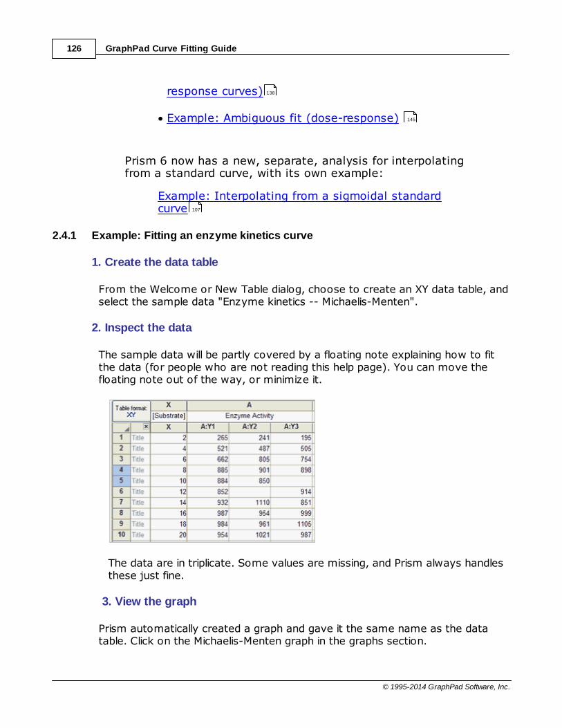
GraphPad Curve Fitting Guide126
© 1995-2014 GraphPad Software, Inc.
response curves)
Example: Ambiguous fit (dose-response)
Prism 6 now has a new, separate, analysis for interpolatingfrom a standard curve, with its own example:
Example: Interpolating from a sigmoidal standardcurve
2.4.1 Example: Fitting an enzyme kinetics curve
1. Create the data table
From the Welcome or New Table dialog, choose to create an XY data table, andselect the sample data "Enzyme kinetics -- Michaelis-Menten".
2. Inspect the data
The sample data will be partly covered by a floating note explaining how to fitthe data (for people who are not reading this help page). You can move thefloating note out of the way, or minimize it.
The data are in triplicate. Some values are missing, and Prism always handlesthese just fine.
3. View the graph
Prism automatically created a graph and gave it the same name as the datatable. Click on the Michaelis-Menten graph in the graphs section.
138
145
107

CURVE FITTING WITH PRISM 6 127
© 1995-2014 GraphPad Software, Inc.
Since this is the first time you are viewing the graph, Prism will pop up theChange Graph Type dialog. Select the fifth choice, to plot individual replicatesrather than mean and error bars.
The graph Prism makes automatically is fairly complete. You can customize thesymbols, colors, axis labels, position of legend, etc.
4. Choose nonlinear regression
Click and choose Nonlinear regression from the list of XY analyses.
Even faster, click the shortcut button for nonlinear regression.
5. Choose a model
On the Fit tab of the nonlinear regression dialog, open the equation folder,Enzyme Kinetics - Substrate vs. Velocity. Then choose the Michaelis-Mentenequation.
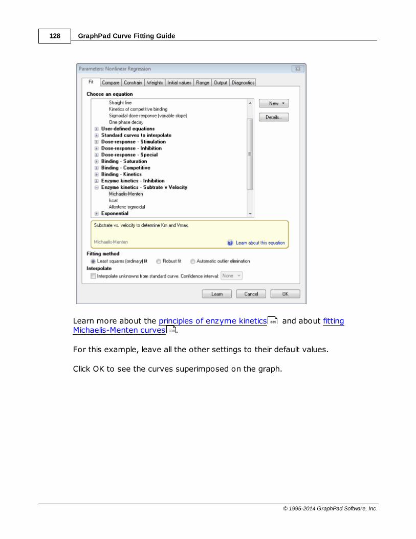
GraphPad Curve Fitting Guide128
© 1995-2014 GraphPad Software, Inc.
Learn more about the principles of enzyme kinetics and about fittingMichaelis-Menten curves .
For this example, leave all the other settings to their default values.
Click OK to see the curves superimposed on the graph.
335
338

CURVE FITTING WITH PRISM 6 129
© 1995-2014 GraphPad Software, Inc.
6. Inspect the graph
7. Inspect the results
The goal of nonlinear regression is to find the best-fit values of the parameters.These are reported at the top of the table. You can't really interpret the best-fitvalues without knowing how precise they are, and this is reported both asstandard errors and confidence intervals . 183

GraphPad Curve Fitting Guide130
© 1995-2014 GraphPad Software, Inc.
8. Go back and perform the replicates test
The replicates test assesses the adequacy of the fit by comparing the scatteramong the triplicates with the scatter of points around the curve. It is notcalculated by default, so the results do not appear in the results of step 7.
You don't have to do the fit over again. Instead click the button in the upper leftcorner of the results table to return to the nonlinear regression dialog.
Go to the Diagnostics tab , and check the option to perform the replicatestest . Note that you can also check an option to make your settings herebecome the default for future fits.
165
194

CURVE FITTING WITH PRISM 6 131
© 1995-2014 GraphPad Software, Inc.
The P value is small (0.013). This means that the scatter of the data from thecurve is greater than you'd expect from the variation among triplicates. Thissuggests that you might want to consider fitting an alternative model, which wedo in the next example .
2.4.2 Example: Comparing two enzyme kinetics models
1.Open analysis parameters dialog
This example continues from the previous one . Click the analysis parameterbutton again.
2. Choose the first model
On the Fit tab, choose (or make sure you still have chosen) the Michaelis-Menten equation.
131
126

GraphPad Curve Fitting Guide132
© 1995-2014 GraphPad Software, Inc.
3. Choose the other model
Go to the Compare tab .
Choose: For each data set, which of two equations (models) fits best?
There are two ways to compare models. For this example, choose the extrasum-of-squares F test .
For the second equation, choose "Allosteric sigmoidal " from the Enzymekinetics section.
157
50
342

CURVE FITTING WITH PRISM 6 133
© 1995-2014 GraphPad Software, Inc.
4. View the results of the model comparison
The top part of the results summarizes the comparison. The P value is low,suggesting that the simpler (Michaelis-Menten) model is too simple and shouldbe rejected. The allosteric model fits significantly better.
5. View the numerical results of the fit to the allosteric model
Scroll down to the best-fit parameter values for the allosteric model.

GraphPad Curve Fitting Guide134
© 1995-2014 GraphPad Software, Inc.
The P value of the replicates test is high, which means the scatter of pointsaround the curve is consistent with variability of replicates from each other.
The parameter H equals 2.0, with a 95% confidence interval ranging from 1.5to 2.5. A value of 2.0 suggests that this enzyme might be a dimer. When Hequals 1.0, the allosteric model is identical to the Michaelis-Menten model.
Further interpretation must, of course, be in the context of what is knownabout this enzyme from prior work. Statistics is only part of analyzing scientificdata.
6. View the graph
Since the allosteric model fit significantly better, that is the model that Prismuses when it plots a curve on the graph. You can barely see that it has asigmoidal shape. You can also see that you should collect more data withsubstrate concentrations between 0 and 5 to fully define this curve.
194

CURVE FITTING WITH PRISM 6 135
© 1995-2014 GraphPad Software, Inc.
2.4.3 Example: Automatic outlier elimination (exponential decay)
Prism implements a unique method to identify outliers when fitting curves withnonlinear regression. This example shows you how easy it is to identify outlierswith Prism. Learn more about how this method works , when it is useful ,and when it should be avoided .
1. Create the data table
From the Welcome or New Table dialog, choose to create XY data table, andselect the sample data "Eliminating outliers during nonlinear regression".
2. Inspect the data table and graph
The data table has values for two data sets (control and treated) with triplicatesubcolumns.
Since this is the first time you are viewing the graph, Prism will pop up theChange Graph Type dialog. Select the fifth choice, to plot individual replicatesrather than mean and error bars.
57 53
54

GraphPad Curve Fitting Guide136
© 1995-2014 GraphPad Software, Inc.
3. Choose nonlinear regression
Click and choose Nonlinear regression from the list of XY analyses.
Alternatively, click the shortcut button for nonlinear regression.
4. Choose a model, and choose automatic outlier detection
On the Fit tab of the nonlinear regression dialog, open the panel of exponentialequations and choose: One phase decay.
Also choose automatic outlier elimination. Learn about when outlier eliminationis helpful , when it should be avoided , and how it works . 53 54 57

CURVE FITTING WITH PRISM 6 137
© 1995-2014 GraphPad Software, Inc.

GraphPad Curve Fitting Guide138
© 1995-2014 GraphPad Software, Inc.
5. View the graph
Prism identified the outlier, and plotted it in red, overlaid on top of the datagraph. After identifying the outlier, Prism fit the remaining data points as if theoutlier wasn't present. Before accepting the results, think about why the pointwas an outlier. Remember, not all outliers are "bad" points .
Double click on the graph to bring up the Format Graph dialog. Go to thesecond tab. You can see that this graph now has three data sets, the data, thecurve fit, and the outliers. Read more about graphing outliers .
2.4.4 Example: Global nonlinear regression (dose-response curves)
1. Create the data table
From the Welcome or New Table dialog, choose to create an XY data table, andselect the sample data "Dose-response: EC50 shift by global fitting". Note thatthis choice is in a drop down menu of sample data sets.
2. Inspect the data
The sample data may be partly covered by a floating note explaining how to fitthe data (for people who are not reading this help page). You can move thefloating note out of the way, or minimize it.
56
176

CURVE FITTING WITH PRISM 6 139
© 1995-2014 GraphPad Software, Inc.
The X values are the logarithm of the concentration of agonist. The Y values areresponses, in duplicate, in two conditions.
3. View the graph
Since this is the first time you are viewing the graph, Prism will pop up theChange Graph Type dialog. Select the first choice, to plot mean and error bars,and choose the kind of error bars you prefer.
4. Choose nonlinear regression
Click and choose Nonlinear regression from the list of XY analyses.
Alternatively, click the shortcut button for nonlinear regression.

GraphPad Curve Fitting Guide140
© 1995-2014 GraphPad Software, Inc.
5. Choose a model
On the Fit tab of the nonlinear regression dialog, open the panel of inhibitorydose-response models and choose: log(inhibitor) vs. response -- variableslope.
For now, leave all the other settings to their default values.
Click OK to see the curves superimposed on the graph.

CURVE FITTING WITH PRISM 6 141
© 1995-2014 GraphPad Software, Inc.
6. Inspect the results
The control results are labeled ambiguous. This means that Prism is unable tofind a unique curve through the data. Lots of other sets of parameter valueswould lead to curves that fit just as well. You can see which parameters areambiguous by looking at the 95% confidence intervals. Instead of reporting aninterval, Prism reports 'very wide' for the Bottom and logEC50.
The data do not define a bottom plateau for the control (circles) data set, so itsbest-fit value is ambiguous. The EC50 is the concentration that gives aresponse half way between the bottom and top plateaus of the curve. If thebottom is ambiguous, so is the EC50.
The treated curve is not labeled 'ambiguous', but the confidence intervals arewider than you'd like.
7. Go back to the dialog, and share three parameters
You can get much better results from this data set if you are willing to assume

GraphPad Curve Fitting Guide142
© 1995-2014 GraphPad Software, Inc.
that that the top and bottom plateaus, and the slope, are the same undercontrol and treated conditions. In other words, you assume that the treatmentshifts the EC50 but doesn't change the basal response, the maximumresponse, or the Hill slope.
Return to the nonlinear regression dialog by clicking the button in the upper leftof the results table.
Go to the constraints tab and choose to share the value of Bottom, Top, andHillSlope. When you share these parameters, Prism fits the data sets globally tofind one best-fit value for Bottom, Top and HillSlope (for both data sets) andseparate best-fit values for the logEC50.
8. View the revised graph and results

CURVE FITTING WITH PRISM 6 143
© 1995-2014 GraphPad Software, Inc.
The fit is no longer labeled 'ambiguous' and the confidence intervals are muchtighter.
9. Statistically compare the two logEC50 values
Go back to the parameters dialog for nonlinear regression and go to theCompare tab. Check the option to test whether one curve adequately fits allthe data sets.
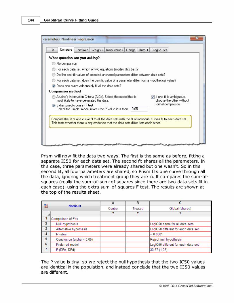
GraphPad Curve Fitting Guide144
© 1995-2014 GraphPad Software, Inc.
Prism will now fit the data two ways. The first is the same as before, fitting aseparate IC50 for each data set. The second fit shares all the parameters. Inthis case, three parameters were already shared but one wasn't. So in thissecond fit, all four parameters are shared, so Prism fits one curve through allthe data, ignoring which treatment group they are in. It compares the sum-of-squares (really the sum-of-sum-of squares since there are two data sets fit ineach case), using the extra sum-of-squares F test. The results are shown atthe top of the results sheet.
The P value is tiny, so we reject the null hypothesis that the two IC50 valuesare identical in the population, and instead conclude that the two IC50 valuesare different.

CURVE FITTING WITH PRISM 6 145
© 1995-2014 GraphPad Software, Inc.
10. Fit the ratio of two IC50 values directly
From the results in step 8, you can compute what you want to know -- theratio of the two EC50 values.
But Prism can calculate this value directly.
Go back to the analysis parameters dialog, and on the Fit tab, change theequation to "EC50 shift" from the "Dose-response - Special" group ofequations. Accept all defaults and click OK. The graph will look identical, as themodel is equivalent. But now, rather than fitting two logEC50 values, Prism fitsone and also fits the ratio.
This equation was designed to do exactly what is needed for this example. Readabout how this equation was set up , so you can construct your ownequations when necessary.
2.4.5 Example: Ambiguous fit (dose-response)
1. Create the data table
From the Welcome or New Table dialog, choose to create XY data table, selectthe sample data "Dose-Response - Ambiguous until constrained". Note that thischoice is in a drop down menu of sample data sets.
279

GraphPad Curve Fitting Guide146
© 1995-2014 GraphPad Software, Inc.
2. Inspect the data table
The X values are the logarithms of molar concentration. The Y values areresponses, entered as mean and SD. With Prism, you can either enter replicatevalues or enter error values (here SD) computed elsewhere.
3. View the graph
Since this is the first time you are viewing the graph, Prism will pop up theChange Graph Type dialog. Select the first choice, to plot mean and error bars,and choose the kind of error bars you prefer.
4. Choose nonlinear regression
Click and choose from the list of XY analyses.
Even faster, click the shortcut button for nonlinear regression.

CURVE FITTING WITH PRISM 6 147
© 1995-2014 GraphPad Software, Inc.
5. Choose a model
On the Fit tab of the nonlinear regression dialog, open the panel of Stimulatorydose-response equations and choose: log(agonist) vs. response -- Variableslope.
Learn more about fitting dose-response curves .
For this example, leave all the other settings to their default values.
Click OK to see the curves superimposed on the graph.
256

GraphPad Curve Fitting Guide148
© 1995-2014 GraphPad Software, Inc.
6. Inspect the graph
The curve goes through the point nicely, and looks fine.
7. Inspect the results
Go to the results page, and view the results.

CURVE FITTING WITH PRISM 6 149
© 1995-2014 GraphPad Software, Inc.
Note the word 'ambiguous' at the top of the results. This means that Prism wasunable to find a unique fit to these data. Lots of sets of parameter values wouldlead to curves that fit just as well. Learn more about ambiguous fits .
Prism does not report confidence intervals for the logEC50 or the Bottom ofthe curve, but instead simply says the intervals are 'very wide'. That tells you itwas impossible to fit those parameters precisely.
While the Y values of the data rum about 100 to about 600, the best-fit valuefor the bottom of the curve is -1067. Furthermore, the best-fit value of thelogEC50 is outside the range of the data.
Even though the curve is close to the points (the R2 is 0.9669), the best-fitparameter values are useless.
8. Constrain the Bottom of the curve
The problem is simple. You have asked Prism to find best-fit value for fourparameters representing the bottom and top plateaus of the curve as well as
228

GraphPad Curve Fitting Guide150
© 1995-2014 GraphPad Software, Inc.
the mid point and steepness. But the data simply don't define the bottom of thecurve. In fact, Prism the best fit value of Bottom is very very far from the data.
These data were calculated so the basal nonspecific response was subtractedaway. This means that you know that the response (Y) at very lowconcentrations of agonist (very low values of X) has to be zero. Prism needs toknow this to fit the data sensibly.
You don't have to do the fit over again. Instead click the button in the upper leftcorner of the results table to return to the nonlinear regression dialog.
Go to the Constrain tab, and check constrain the parameter Bottom to have aconstant value which you set to 0.0.
9. Inspect the revised results
Now the results make sense. The logEC50 is in the middle of the range of Xvalues. The confidence intervals are reasonably tight. And, of course, the resultsare no longer 'ambiguous'.

CURVE FITTING WITH PRISM 6 151
© 1995-2014 GraphPad Software, Inc.
2.5 Nonlinear regression with Prism
Prism's nonlinear regression dialog has seven tabs, explainedhere. It can seem overwhelming at first. But you don't have tolearn about all the choices when you first fit a curve. Start byfocussing on the choices in the first (Fit) tab, and then learnabout the other choices later.
Before learning all the details, first understandthe big picture -- the basic steps required tofit a model to data.
So many choices! Which ones are essential?
152
154

GraphPad Curve Fitting Guide152
© 1995-2014 GraphPad Software, Inc.
2.5.1 How to fit a model with Prism
Step 1. Enter data
Create an XY table, and enter data. If you have replicate Y values at each Xvalue, format the table for entry of replicates.
From an XY table or graph, click the shortcut button to fit a model withnonlinear regression. Or click Analyze and select from the analyze dialog.
Step 2. Choose a model
Nonlinear regression fits a model to your data. You must, therefore, choose amodel or enter a new model.
Why a computer program cannot pick a model for you .
Step 3. Choose (or review) initial values
Nonlinear regression is an iterative procedure. The program must start withestimated values for each variable that are in the right "ball park" - say within afactor of five of the actual value. It then adjusts these initial values to improvethe fit. See How nonlinear regression works.
GraphPad Prism provides initial values automatically if you use a built-inequation. If you enter your own equation, you can also enter rules for initialvalues. For example the initial value of one parameter may be twice themaximum Y value in the data, while the initial value of another parameter mayequal the average of the highest and lowest X values. Once you define theserules, Prism will compute appropriate initial values based on the range of yourdata.
The Initial Values tab of the Nonlinear regression dialog lets you review, andoverride, the computed initial values.
You'll find it easy to estimate initial values if you have looked at a graph of thedata, understand the model, and understand the meaning of all the parametersin the equation. Remember that you just need an estimate. It doesn't have to
12
162

CURVE FITTING WITH PRISM 6 153
© 1995-2014 GraphPad Software, Inc.
be very accurate. If you are having problems estimating initial values, set asideyour data and simulate curves using the model. Change the variables one at atime, and see how they influence the shape of the curve. Once you have abetter feel for how the parameters influence the curve, you might find it easierto estimate initial values.
When fitting a simple model to clean data, it won't matter much if the initialvalues are fairly far from the correct values. You'll get the same best-fit curveno matter what initial values you use, unless the initial values are extremely farfrom correct. Initial values matter more when your data have a lot of scatter oryour model has many variables.
Step 4. Decide whether to constrain any parameters
When performing nonlinear regression, you don't have to fit each parameter inthe equation. Instead, you may fix one or more of the parameters to constantvalues. It is often helpful to define constants when you have only a few datapoints. For example, you might fix the bottom plateau of a sigmoid curve orexponential decay to zero.
Remember that nonlinear regression programs have no "common sense". Youneed to think about how you did the experiment, and decide whether some ofthe parameters should be fixed. For example, if a background signal has alreadybeen subtracted, it makes sense to fix the bottom plateau of a dose-responsecurve or an exponential decay curve to zero.
Prism also let you constrain parameters to a certain range of values.
Step 5. If you are fitting two or more data sets at once, decide whether toshare any parameters
If you enter data into two or more data set columns, Prism will fit them all inone analysis. But each fit will be independent of the others unless you specifythat one or more parameters are shared. When you share parameters, theanalysis is called a global nonlinear regression .
Step 6. Decide on a weighting scheme
Nonlinear regression programs generally weight each point equally. But thereare many ways to differentially weight the points .
Step 7. Choose other options
Read about choices on the Range , Output and Diagnostics tab.
41
160
164 164 165

GraphPad Curve Fitting Guide154
© 1995-2014 GraphPad Software, Inc.
2.5.2 Which choices are essential?
So many choices! Prism's nonlinear regression dialog has seven tabs, and canseem overwhelming at first. But you don't have to learn about all the choiceswhen you first fit a curve.
If your goal is to fit a standard curve from which to interpolate unknown values
If your goal is to interpolate from a standard curve, you can ignore most of thechoices that Prism offers. You do need to pick a model, but you should judgethe adequacy of the model visually. If it goes through the points withoutwiggling too much, it is fine for interpolation. Note that Prism 6 offers a simplified curve fitting analysis for interpolation .
If your goal is to fit a model to determine best-fit parameters
If your goal is to fit a model to determine parameter values, then choosing amodel is the essential first step. You should not expect a computer (or asoftware company's tech support) to choose a model for you. Choosing amodel, and deciding which parameters should be constrained and which shouldbe shared among data sets, is a scientific decision that is fundamental toanalyzing your data. The other choices are useful, but can be put aside whenyou are first learning curve fitting..
2.5.3 Nonlinear regression choices
Choose the model (equation) on the Fit tab . This is also where youchoose to eliminate outliers and to interpolate values from the fitcurve.
Compare tab . Choose to compare the fit of two modelsto each data set, or to compare the fit of two (or more)data sets.
Constrain tab . Fix parameter values to constant valuesand/or designate parameters to be shared among all datasets.
There are many situations where you don't want to weightall points equally. Set unequal weighting on the Weightstab .
105
155
157
158
160

CURVE FITTING WITH PRISM 6 155
© 1995-2014 GraphPad Software, Inc.
Nonlinear regression is an iterative procedure. The programmust start with estimated initial values for each parameter.It then adjusts these initial values to improve the fit. Viewthose values on the Initial values tab .
Range tab . Set the X range of data to fit, the startingand ending X values for the plotted curve, and whether youwant to view a table of XY coordinates that define thecurve.
Output tab
Diagnostics tab . Prism can create more detailed resultstables.
2.5.3.1 Fit tab
Choose an equation
Selecting an equation is the most important step in fitting a curve. The choice cannot be automated .
If your goal is to fit a model in order to understand your data and makecomparisons, then choosing a model is a scientific decision that you must makewith care. If your goal is to interpolate unknowns from a standard curve, then itmatters less which equation you pick, so long as it ends up creating a smoothcurve through your data.
Some tips:
Prism provides a long list of equations that you can choose. But if these don't
fit your needs, don't be afraid to create or clone an equation to fit yourneeds.
Part of choosing a model is choosing constraints . Don't skip that step. For
example, if you choose a sigmoidal dose response model, you must decidewhether you wish Prism to find the best fit value of the bottom plateau basedon the trend of the data. The alternative is to constrain the bottom plateau toequal zero, if you have subtracted off a baseline, or some other value(defined by controls). A computer can't make these decisions for you.Choosing which constraints to apply to your model is a fundamental decisionin data analysis that can have a huge impact on the results.
If you are fitting several data sets at once, part of choosing a model is
162
164
164
165
12
409
158
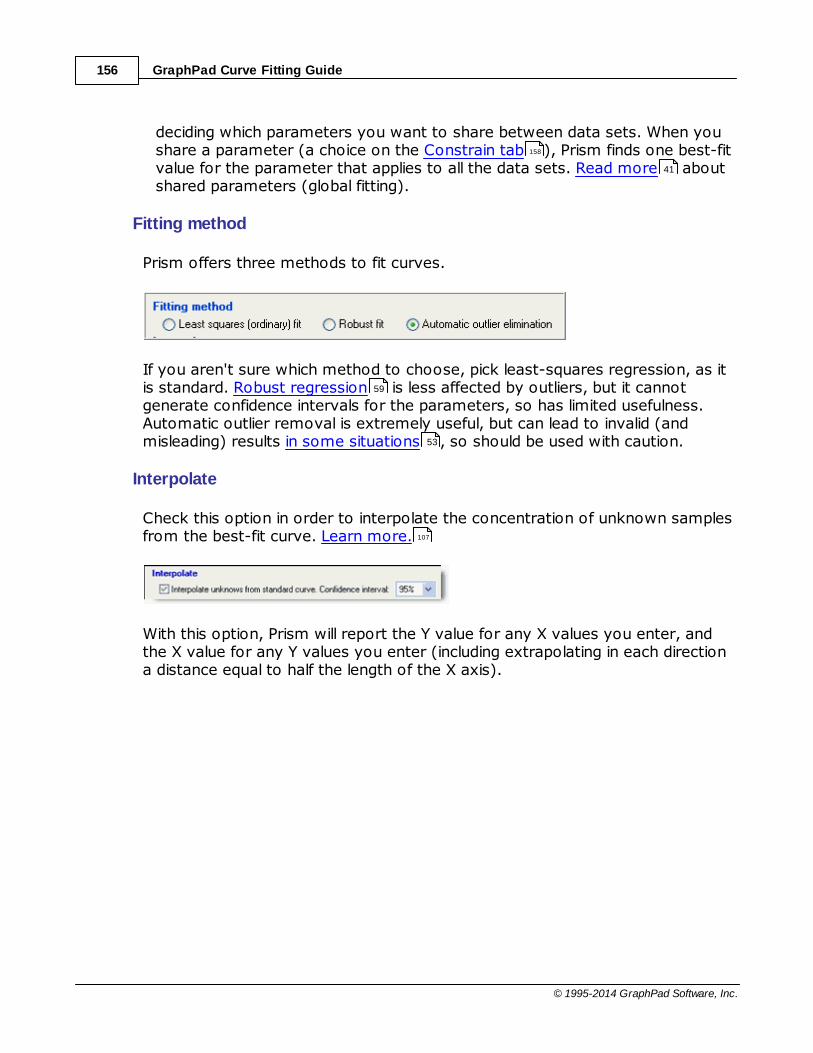
GraphPad Curve Fitting Guide156
© 1995-2014 GraphPad Software, Inc.
deciding which parameters you want to share between data sets. When youshare a parameter (a choice on the Constrain tab ), Prism finds one best-fitvalue for the parameter that applies to all the data sets. Read more aboutshared parameters (global fitting).
Fitting method
Prism offers three methods to fit curves.
If you aren't sure which method to choose, pick least-squares regression, as itis standard. Robust regression is less affected by outliers, but it cannotgenerate confidence intervals for the parameters, so has limited usefulness.Automatic outlier removal is extremely useful, but can lead to invalid (andmisleading) results in some situations , so should be used with caution.
Interpolate
Check this option in order to interpolate the concentration of unknown samplesfrom the best-fit curve. Learn more.
With this option, Prism will report the Y value for any X values you enter, andthe X value for any Y values you enter (including extrapolating in each directiona distance equal to half the length of the X axis).
158
41
59
53
107

CURVE FITTING WITH PRISM 6 157
© 1995-2014 GraphPad Software, Inc.
2.5.3.2 Compare tab
When fitting biological data with regression, your main objective is often todiscriminate between different models, to ask if an experimental interventionchanged a parameter, or to ask if the best-fit value of a parameter differssignificantly from a theoretical value. Learn more about these four kinds ofcomparisons . Your choice, of course, has to be based on your experimentalgoals.
Prism can perform the comparison using two alternative methods : the extrasum-of-squares F test , and using Akaike's information criteria . Use theseguidelines to choose:
In most cases, the two models will be 'nested'. This means that one model is
a simpler case of the other. For example, a one-phase exponential model is asimpler case of a two-phase exponential model. Either the F test or the AICcmethod may be used with nested models. The choice is usually a matter ofpersonal preference and tradition. Basic scientists in pharmacology andphysiology tend to use the F test. Scientists in fields like ecology andpopulation biology tend to use AICc.
If the models are not nested, then the F test is not valid so you should
choose AICc. Note that Prism does not enforce this. It will calculate the F testeven if the models are not nested, but the results won't be useful.
Both these methods only make sense when the models being compared havedifferent numbers of parameters, and so have different numbers of degrees offreedom. If you want to compare two models with the same number ofparameters, there is no need to use either the F test or AIC. Simply choose themodel that fits the data the best with the smallest sum-of-squares.
46
48
50 51

GraphPad Curve Fitting Guide158
© 1995-2014 GraphPad Software, Inc.
2.5.3.3 Constrain tab
The importance of constraints
Prism lets you constrain each parameter to a constant value, constrain to a range ofvalues, share among data sets (global fit), or define a parameter to be a columnconstant. This is an important decision, and will influence the results.
Constrain to a constant value
You won't always want to fit all the parameters in a model. Instead, you can fixone or more parameters to constant values. For example, if you havenormalized a dose-response curve to run from 0 to 100, constrain Top toequal 100 and Bottom to 0.0. Similarly, if you have subtracted a baseline soyou know that the exponential decay curve has to plateau at Y=0.0, you canconstrain the Bottom parameter to equal 0.0.
Deciding to constrain a parameter to a constant value can make a hugedifference in the results. Remember Prism has no common sense. It doesn'tknow if a curve has to plateau at zero unless you tell it.
Constrain to a range of values
Constrain to a range of values to prevent Prism from letting parameters takeon impossible values. For example, you should constrain rate constants to onlyhave values greater than 0.0, and fractions (say the fraction of binding sitesthat are high affinity) that have a value between 0.0 and 1.0. Setting this kindof constraint can have four outcomes:
The constraint is irrelevant, as the parameter never would have taken on a
value in the forbidden range.
The constraint helped speed up the fit. Nonlinear regression works by
iteratively changing the values of the parameters. With some complicatedfits, the nonlinear regression process can 'get confused' and end upspending time exploring parameter values that make no sense. Constraining

CURVE FITTING WITH PRISM 6 159
© 1995-2014 GraphPad Software, Inc.
the values of one or more parameters can prevent the nonlinear regressionprocess from being led astray. With huge numbers of data points, you mightsee a noticeable speeding up of the fitting process.
The constraint helped nonlinear regression choose from several local
minima. Nonlinear regression works by changing parameter values step bystep until no small change affects the sum-of-squares (which quantifiesgoodness-of-fit). With some models, there can be two sets of parametervalues that lead to local minima in sum-of-squares. Applying a constraintcan ensure that nonlinear regression finds the minimum with scientificallyrelevant values, and ignores another minimum that fits the curve well butusing parameter values that make no scientific sense (i.e. negativeconcentrations).
The constraint prevents nonlinear regression from finding a minimum sum-
of-squares. Instead, the best the program can do (while obeying theconstraint) is set the parameter to the limit of the constrained range. Prismthen reports that the fit 'hit constraint'.
In the first case, the constraint is harmless but useless.
In the next two cases, the constraint helps the nonlinear regression reachsensible results. Essentially, the constraint can give the nonlinear regressionprocess some scientific judgment about which parameter values are simplyimpossible. These cases are really what constraints are for.
The last case, when the fit ends with a parameter set to one end of itsconstraint, it is tricky to interpret the results.
Sharing parameters among data sets. Global nonlinear regression.
If you are fitting a family of curves, rather than just one, you can choose to sharesome parameters between data sets. For each shared parameter, Prism findsone (global) best-fit value that applies to all the data sets. For each non-sharedparameter, the program finds a separate (local) best-fit value for each data set.Global fitting is a very useful tool in two situations:
The parameter(s) you care about are determined from the relationship
between several data sets. Learn more.
Each dataset is incomplete, but the entire family of datasets defines the
parameters. See example.
231
43
42

GraphPad Curve Fitting Guide160
© 1995-2014 GraphPad Software, Inc.
Data set constant
When you fit a family of curves at once, you can set one of the parameters tobe a data set constant.Prism offers two data set constants.
Column title. The value comes from the column title, which can be differentfor every data set. This parameter becomes almost a second independentvariable. It has a constant value within any one data set, but a different valuefor each data set. For example, when fitting a family of enzyme progresscurves in the presence of various concentrations of inhibitor, the inhibitorconcentration can be entered into the column title of the data table. View anexample .
Mean X. The value is the mean of all the X values for which there are Y valuesin that data set. This is used in centered polynomial regression.
2.5.3.4 Weights tab
ROUT coefficient
If you ask Prism to automatically exclude outliers (a choice on the Fit tab) or tocount (but not remove from the analysis) outliers (a choice on the Diagnosticstab), set the ROUT coefficient to determine how aggressively Prism definesoutliers.
We recommend using a value of 1%. Our simulations have shown that if all thescatter is Gaussian, Prism will falsely find one or more outliers in about 2-3% ofexperiments. If there really are outliers present in the data, Prism will detectthem with a False Discovery Rate less than 1%. See reference 1.
If you set Q to a higher value, the threshold for defining outliers is less strict.This means that Prism will have more power to detect outliers, but also willfalsely detect 'outliers' more often. If you set Q to a lower value, the thresholdfor defining outliers is stricter. This means that Prism will have a less power todetect real outliers, but also have a smaller chance of falsely defining a point tobe an outlier.
If you set Q to 0, Prism will fit the data using ordinary nonlinear regressionwithout outlier identification.
424

CURVE FITTING WITH PRISM 6 161
© 1995-2014 GraphPad Software, Inc.
Unequal weighting
It is often useful to differentially weight the data points. Learn why.
Prism offers seven choices on the Weight tab of nonlinear regression:
No weighting. Regression is most often done by minimizing the sum-of-squares of the vertical distances of the data from the line or curve. Pointsfurther from the curve contribute more to the sum-of-squares. Points close tothe curve contribute little. This makes sense, when you expect experimentalscatter to be the same, on average, in all parts of the curve.
Weight by 1/Y^2. In many experimental situations, you expect the averagedistance (or rather the average absolute value of the distance) of the pointsfrom the curve to be higher when Y is higher. The points with the larger scatterwill have much larger sum-of-squares and thus dominate the calculations. Ifyou expect the relative distance (residual divided by the height of the curve) tobe consistent, then you should weight by 1/Y2.
Weight by 1/Y. This choice is useful when the scatter follows a Poissondistribution -- when Y represents the number of objects in a defined space orthe number of events in a defined interval.
Weight by 1/YK. Also called "General weighting". Read more.
Weight by 1/X or 1/X2 .These choices are used rarely. Only choose theseweighting schemes when it is the standard in your field, such as a linear fit of abioassay.
Weight by 1/SD2. If you enter replicate Y values at each X (say triplicates), itis tempting to weight points by the scatter of the replicates, giving a point lessweight when the triplicates are far apart so the standard deviation (SD) is high.But unless you have lots of replicates, this doesn't help much. The triplicatesconstituting one mean could be far apart by chance, yet that mean may be asaccurate as the others. Weighting needs to be based on systematic changes inscatter. The choice to weight by 1/SD2 is most useful when you want to use aweighting scheme not available in Prism. In this case, enter data as mean andSD, but enter as "SD" weighting values that you computed elsewhere for thatpoint. In other words, the values you enter in the SD subcolumn are notactually standard deviations, but are weighting factors computed elsewhere.
Notes on weighting
If you have normalized your data, weighting rarely makes sense.
30
31

GraphPad Curve Fitting Guide162
© 1995-2014 GraphPad Software, Inc.
Simulations can show you how much difference it makes if you choose the
wrong weighting scheme.
If you choose unequal weighting, Prism takes this into account when
plotting residuals.
Prism accounts for weighting when it computes R 2 .
Learn about the math of weighting and how Prism does the weighting .
Replicates
In most experiments, it is fair to consider each replicate to be an independentdata point, and you should choose that first choice unless you have a strongreason not to.
Here is an example where you would want to fit only the means: Youperformed a dose-response experiment, using a different animal at each dosewith triplicate measurements. The three measurements are not independent. Ifone animal happens to respond more than the others, that will affect all thereplicates. Since the replicates are not independent, you should fit the means.
Reference
1. Motulsky HM and Brown RE, Detecting outliers when fitting data withnonlinear regression – a new method based on robust nonlinear regressionand the false discovery rate, BMC Bioinformatics 2006, 7:123..
2.5.3.5 Initial values tab
Why initial values?
Nonlinear regression is an iterative procedure. The program must start with estimatedinitial values for each parameter. It then adjusts these initial values to improve the fit.
How does Prism provide initial values automatically?
Every equation built-in to Prism, as well as equations you define, include rules to
179
187187
31 65

CURVE FITTING WITH PRISM 6 163
© 1995-2014 GraphPad Software, Inc.
compute initial values. These rules use the range of the X and Y values to comeup with initial values, which become the original automatic initial values. Youcan change the rules for user-defined equations, and can clone built-inequations to make them user-defined. The new rules will be invoked when younext choose this equation for a new analysis. It won't change the initial valuesfor the analysis you are working on.
Are the initial values reasonable?
If nonlinear regression doesn't report any results, or if they seem wrong, the problemmight be bad initial values. To check whether the initial values are reasonable, check"Don't fit the curve. Instead plot the curve defined by initial values." on theDiagnostics tab. When you click OK from the nonlinear regression dialog, Prism will not fita curve but will instead generate a curve based on your initial values. If this curve is notgenerally in the vicinity of the data points, change the initial values before runningnonlinear regression.
Changing the initial values
In most cases, the automatic initial values will work fine. If you have trouble getting asensible fit, you might need to tweak the initial values. You can override the automaticinitial values for each parameter for each data set:
1. Select a data set on the top part of the initial values tab. Or hold down the Ctrl keyand select several data sets. Or click "Select all" in the top right of the tab.
2.Uncheck "choose automatically" and enter the new initial value.
you will find it easy to estimate initial values if you have looked at a graph of the data,understand the model, and understand the meaning of all the parameters in theequation. Remember that you just need an estimate. It doesn't have to be veryaccurate.
How much difference do initial values make?
When fitting a polynomial model, it makes no difference what values you enteras initial values. When fitting other models, the importance of the initial valuesdepends on how well the data define the curve and on how many parametersare in the model. Initial values matter the most when your data have a lot ofscatter and don't define the model very well, and your model has manyparameters.
433

GraphPad Curve Fitting Guide164
© 1995-2014 GraphPad Software, Inc.
2.5.3.6 Range tab
Ignore points outside of a specified X range
If you choose these options nonlinear regression will completely ignore all datawhere the X value is less than, or larger than, the thresholds you set. This couldbe useful if you collect data over time, and only want to fit data within a certainrange of time points.
Define the curve
In addition to fitting the model to your data, Prism also superimposes the curveon your graph. Choose where the curves should begin and end.
Table of XY coordinates
Check this option if you want to see a table of XY coordinates of line segmentsdefining the curve.
In prior versions of Prism, this table was critical to plotting the curve andinterpolating unknowns. But Prism 5 can graph the curve and interpolateunknowns from the curve, without creating this table. Check the option tocreate this table only if you want to copy (or export) the table into anotherprogram. In most cases, you will have no need to view this table, and so shouldleave the option unchecked.
2.5.3.7 Output tab
Summary table
When analyzing several data sets, the results table is rather lengthy. To displaykey results on a summary table, check the option box to create a summarytable and select the variable you wish to summarize. Prism creates a summarytable (as an additional results view) that shows the best-fit value of thatparameter for each data set, and graphs this table.
Depending on your choices in the dialog, this may be a bar graph or an XYgraph. It shows the best-fit value of a selected parameter for each data set onthe table. In some cases, you may analyze the summary table with linear ornonlinear regression. For example, the summary graph may show the best-fitvalue of a rate constant as a function of concentration (obtained from thecolumn titles of the original data). You can fit a line or curve to that graph.
When Prism compares the fits of two equations, it shows only the results forthe second equation. Since this may not be helpful, we suggest that you only

CURVE FITTING WITH PRISM 6 165
© 1995-2014 GraphPad Software, Inc.
make summary tables when fitting a single equation.
Number of digits in output
Choose how many significant digits you want to see in the main results table.This is especially useful if you embed the results table on a graph or layout.
For the table of residuals and the curve itself, you can choose a number formatby selecting column(s) and bring up the Decimal Format dialog.
Additional output
Prism offers two options here (dose ratios, and Ki from IC50). These areavailable only to be compatible with earlier versions of Prism (so Prism canopen files made with older versions). They are almost always unavailable,becoming available only if you select certain equations from the classicequations list.
Since Prism 5, you can calculate a Gaddum/Schild EC50 shift directly, withoutneed to separately compute dose ratios. Similarly, you can fit competitivebinding curves directly to determine the Ki for one or two sites, without aseparate Cheng-Prusoff calculation of Ki from IC50(1).
1. Cheng, Y. and Prusoff, W. H. Relationship between the inhibition constant(K1) and the concentration of inhibitor which causes 50 per cent inhibition (I50)of an enzymatic reaction. Biochem Pharmacol, 22: 3099-3108, 1973.
2.5.3.8 Diagnostics tab
Do the initial parameter values define a curve near the data?
Nonlinear regression works iteratively, and begins with initial values for eachparameter. Check "don't fit the curve" to see the curve generated by your initialvalues. If the curve is far from the data, go back to the initial parameters taband enter better values for the initial values. Repeat until the curve is near thepoints. Then go back to the Diagnostics tab and check "Fit the curve". This is
277
312 317
162

GraphPad Curve Fitting Guide166
© 1995-2014 GraphPad Software, Inc.
often the best way to diagnose problems with nonlinear regression.
While fitting a curve, Prism will stop after the maximum number of iterations sethere. If you are running a script to automatically analyze many data tables, youmight want to lower the maximum number of iterations so Prism won't wastetime trying to fit impossible data.
How precise are the best-fit values of the parameters?
If your goal is to find the best-fit value of the parameters, you will also want toknow how precise those estimates are. We suggest that you report confidence intervals, as inspecting the confidence intervals of best-fitparameters is an essential part of evaluating any nonlinear fit. Standard errorsare intermediate values used to compute the confidence intervals, but are notvery useful by themselves. Include standard errors in the output to comparePrism's results to those of another program that doesn't report confidenceintervals.
Choose to report confidence intervals as a range or separate blocks of lowerand upper confidence limits (useful if you want to paste the results into anotherprogram).

CURVE FITTING WITH PRISM 6 167
© 1995-2014 GraphPad Software, Inc.
-9 -8 -7 -6 -5 -4 -3
0
500
1000
1500
log(Dose)
Resp
on
se
95% confidence band
-9 -8 -7 -6 -5 -4 -3
0
500
1000
1500
log(Dose)
Resp
on
se
95% prediction band
The 95% confidence bands enclose the area that you can be 95% surecontains the true curve. It gives you a visual sense of how well your data definethe best-fit curve.
The 95% prediction bands enclose the area that you expect to enclose 95%of future data points. This includes both the uncertainty in the true position ofthe curve (enclosed by the confidence bands), and also accounts for scatter ofdata around the curve. Therefore, prediction bands are always wider thanconfidence bands. When you have lots of data points, the discrepancy is huge.
Learn more about confidence and prediction bands.
How to quantify goodness-of-fit
You will probably want to ask Prism to report R2 , simply because it isstandard to do so, even though knowing R2 doesn't really help you interpret theresults. Reporting the sum-of-squares and s
y.x will only be useful if you want to
compare Prism's results to those of another program, or you want to doadditional calculations by hand.
The adjusted R 2 takes into account the number of parameters fit to thedata, so has a lower value than R2 (unless you fit only one parameter, in whichcase R2 and adjusted R2 are identical).
Prism also lets you choose to report the AICc . This would be useful only ifyou separately fit the same data to three or more models. You can then usethe AICc to choose between them. But note that it only makes sense tocompare AICc between fits, when the only difference is the model you chose. Ifthe data or weighting are not identical between fits, then the comparison ofAICc values would be meaningless.
200
187
190190
51

GraphPad Curve Fitting Guide168
© 1995-2014 GraphPad Software, Inc.
Normality tests
Least-squares nonlinear regression assumes that the distribution of residualsfollows a Gaussian distribution (robust nonlinear regression does not make thisassumption). Prism can test this assumption by running a normality test onthe residuals. Prism offers three normality tests. We recommend theD'Agostino-Pearson test.
Does the curve systematically deviate from the points?
Does the curve follow the trend of the data? Or does the curve systematicallydeviate from the trend of the data? Prism offers two tests that answer thesequestions.
If you have entered replicate Y values, choose the replicates test to find outif the points are 'too far' from the curve (compared to the scatter amongreplicates). If the P value is small, conclude that the curve does not come closeenough to the data.
The runs test is available if you entered single Y values (no replicates) orchose to fit only the means rather than individual replicates (weighting tab). A'run' is a series of consecutive points on the same side of the curve. If there aretoo few runs, it means the curve is not following the trend of the data.
If you choose a residual plot , Prism creates a new graph. The X axis is thesame as the graph of the data, while the Y axis plots the distance of each pointfrom the curve (the residuals). Points with positive residuals are above thecurve; points with negative residuals are below the curve. Viewing a residualplot can help you assess whether the distribution of residuals is random aboveand below the curve.
185
194
193
179

CURVE FITTING WITH PRISM 6 169
© 1995-2014 GraphPad Software, Inc.
Are the parameters intertwined or redundant or skewed?
What does it mean for parameters to be intertwined? After fitting a model,change the value of one parameter but leave the others alone. The curvemoves away from the points. Now, try to bring the curve back so it is close tothe points by changing the other parameter(s). If you can bring the curve closerto the points, the parameters are intertwined. If you can bring the curve backto its original position, then the parameters are redundant. In this case, Prismwill alert you by labeling the fit 'ambiguous' .
We suggest that you report the dependency , and not bother with thecovariance matrix . When you are getting started with curve fitting, it is OK toleave both options unchecked.
Even though nonlinear regression, as its name implies, is designed to fitnonlinear models, some of the inferences actually assume that some aspects ofthe model are close to linear, so that the distribution of each parameter issymmetrical. This means that if you analyzed many data sets sampled from thesame system, the distribution of the best-fit values of the parameter would besymmetrical and Gaussian.
If the distribution of a parameter is highly skewed, the reported SE and CI forthat parameter will not be very useful ways of assessing precision. Hougaard'smeasure of skewness quantifies how skewed each parameter is.
Could outliers impact the results?
Nonlinear regression is based on the assumption that the scatter of dataaround the ideal curve follows a Gaussian distribution. The presence of one or afew outliers (points much further from the curve than the rest) can overwhelmthe least-squares calculations and lead to misleading results.
Check this option to count the outliers, but leave them in the calculations.Choose how aggressively to define outliers by adjusting the ROUT coefficient.
If you chose the option in the Fit tab to exclude outliers from thecalculations, then this option to simply count outliers (in the Diagnostics tab) isnot available.
228
197
197
204
160
155

GraphPad Curve Fitting Guide170
© 1995-2014 GraphPad Software, Inc.
Would it help to use stricter convergence criteria?
Nonlinear regression is an iterative process. It starts with initial values of theparameters, and then repeatedly changes those values to increase thegoodness-of-fit. Regression stops when changing the values of the parametersmakes a trivial change in the goodness of fit.
Prism lets you define the convergence criteria in three ways. The mediumchoice is default, and will work fine in most cases. With this choice, nonlinearregression ends when five iterations in a row change the sum-of-squares byless than 0.0001%. If you are having trouble getting a reasonable fit, you mightwant to try the stricter definition of convergence: five iterations in a rowchange the sum-of-squares by less than 0.00000001%. It won't help veryoften, but is worth a try. The only reason not to always use the strictest choiceis that it takes longer for the calculations to complete. That won't matter withsmall data sets, but will matter with large data sets or when you run scripts toanalyze many data tables.
If you are fitting huge data sets, you can speed up the fit by using the 'quick'definition of convergence: Two iterations in a row change by less than 0.01%.
2.5.4 Graphing tips: Nonlinear regression
Prism automatically graphs the best-fit curves from nonlinearregression, and you'll rarely need to think about this step.
Tips on graphing curves
Graphing prediction and confidence bands
Adding an equation , or a table of best-fitparameters, to the graph.
Graphing outliers .
Graphing residuals .
162
171
171
175
176
179
CURVE FITTING WITH PRISM 6 171
© 1995-2014 GraphPad Software, Inc.
2.5.4.1 Graphing best-fit curves
Automatic vs. manual plotting
When Prism performs nonlinear regression, it automatically superimposes thecurves on the graph.
If you need to create additional graphs, or change which curve is plotted onwhich graph, keep in mind that from Prism's point of view, a curve generatedby nonlinear regression is simply a data set. You can add curves to a graph orremove curves from a graph on the 'Data on graph' tab of the Format Graphdialog.
Plotting curves after comparing models
If you ask Prism to compare two models, only the selected model is graphed. Ifyou want to graph both models, you will need to analyze the data twice, oncewith each model.
Plotting on logarithmic axes
With Prism 5 and 6, it is Ok to stretch an axis to a log scale, a choice on top ofthe Format Axis dialog. With prior versions, this didn't work well. The curve wasdefined as a series of line segments, and these would be far from equallyspaced on a log axis. Prism 5 and 6 are smarter, so the curve will look smoothon either a linear or logarithmic axis.
Plotting only a portion of the curve
Let's say that the X values of your data range from 0 to 100, and you fit acurve with nonlinear regression. Now you want to create a graph showing onlythe data with X values between 0 and 10. The curve will look ragged. Theproblem is that Prism defines the entire curve using 150 line segments. In thisexample, you only plot 10% of the range, so the curve will have only 15 linesegments.
To fix this problem, go to the Range tab of nonlinear regression and choose todefine the curve with more line segments. In this example, increasing the valuetenfold, to 1500, would be about right.
2.5.4.2 Graphing confidence and prediction bands
The difference between confidence and prediction bands
The 95% confidence bands enclose the area that you can be 95% sure

GraphPad Curve Fitting Guide172
© 1995-2014 GraphPad Software, Inc.
contains the true curve. It gives you a visual sense of how well your data definethe best-fit curve.
The 95% prediction bands enclose the area that you expect to enclose 95%of future data points. This includes both the uncertainty in the true position ofthe curve (enclosed by the confidence bands), and also accounts for scatter ofdata around the curve.
Choose in the Diagnostics tab of the Nonlinear regression parameters dialog.Learn how they are calculated .
Prediction bands are always wider than confidence bands. When you have lotsof data points, the discrepancy is huge.
-9 -8 -7 -6 -5 -4 -3
0
500
1000
1500
log(Dose)
Resp
on
se
95% confidence band
-9 -8 -7 -6 -5 -4 -3
0
500
1000
1500
log(Dose)
Resp
on
se
95% prediction band
Plotting confidence or prediction bands
After you choose to create a confidence or prediction band in the diagnosticstab, it should just appear on the graph. You can fine tune its appearance on thegraph. Note the following:
The fit curve is seen by the Format Graph dialog as one more data set to
plot. be sure to select one of those nonlinear fits first (top of dialog) beforeadjusting its properties.
To plot the confidence bands, choose to show error bars, and set the style to
------ or _____.
You can also choose to show an area fill within the error bands.
165
67

CURVE FITTING WITH PRISM 6 173
© 1995-2014 GraphPad Software, Inc.
Why do so many points lie outside the confidence bands?
Confidence bands show you how well you know the location of the best fit lineor curve. Given all the assumptions of the analysis, you can be 95% sure thatthe true curve (nonlinear regression) or line (linear regression) lies within thebands.
Prediction bands show you where you can expect the data to lie. You expect95% of all data points to lie within the prediction bands.
With many data points, you expect a large fraction of the data points to lieoutside the confidence band, but 95% to lie within the prediction bands. Theconfidence bands aren't supposed to show you the scatter of the data, butrather the uncertainty in the position of the line or curve. With lots of data, theline or curve is known fairly precisely, so only a small fraction of data lie withinthe bands. The figure below demonstrates this with linear regression.

GraphPad Curve Fitting Guide174
© 1995-2014 GraphPad Software, Inc.
Plotting both confidence and prediction bands
Prism lets you choose either a confidence band or a prediction band as part onthe diagnostics tab . But not both. To plot both on one graph, analyze yourdata twice, choosing a confidence band the first time and a prediction band thesecond time. The curves are data sets that you can add to any graph by drag-n-drop or using the Change menu from the graph.
One-sided confidence (or prediction) bands
Confidence and prediction bands are usually two-sided. But you can get Prismto show the band on only one side.
One use for a one-sided confidence band would be on a graph that plots purityof a substance over time. You want to know, with a certain confidence, howlow the purity could be at a certain time. You don't really care about quantifyinghow high the purity could be.
To plot a one-sided 95% confidence (or prediction) band:
1.Choose "90%" confidence bands in the Diagnostics tab of the nonlinearregression dialog. With 90% bands, there is a 5% chance that the true valueis larger than the upper band, and 5% it is lower than the lower band. Whenyou plot only one of these bands, therefore, it is really a 95% confidenceband, which is probably what you want.
2.On the Format Symbols dialog, choose the best-fit line or curve and makesure that error bars are turned on with the "---" style. Then choose either Upor Down (but not Both) in the Direction drop-down menu.
165
CURVE FITTING WITH PRISM 6 175
© 1995-2014 GraphPad Software, Inc.
Viewing the XY coordinates of confidence or prediction bands
1.Go to the Diagnostics tab and check the option to plot confidence orprediction bands.
2.Go to the Range tab of the nonlinear regression dialog.
3.Check the option to create a table of XY coordinates. This table will includethe confidence or prediction bands.
4.When viewing the results, expand the results sheet in the navigator and go tothe page labeled 'Curve'. For each X value, you'll see the y value and thedistance the confidence or prediction curve is above and below that value.
Why won't Prism plot confidence or prediction bands?
Prism will not plot confidence or prediction bands in several situations:
If the best-fit value of a parameter hit a constraint , the fit is unlikely to be
useful. Prism does not plot confidence or prediction bands, because theywould almost certainly be misleading.
If the results of nonlinear regression are ambiguous , the confidence or
prediction bands would be super wide, maybe infinitely wide. They would notbe useful, so Prism does not plot them.
If you choose robust nonlinear regression, Prism does not compute
confidence or prediction bands, as it cannot compute standard errors orconfidence intervals of the parameters.
The fit is perfect . If the sum-of-squares is 0.0 and R2 is 1.0, it is not
possible to compute or interpret confidence or prediction bands.
If the fit is interrupted , confidence and prediction bands are not computed.
2.5.4.3 Adding the equation to the graph
Prism does not automatically write equations on the graph. There are twoapproaches you can use to do so.
Microsoft Office comes with an equation editor. If Microsoft Equation Editor isinstalled on your system, you will see a quick-access button on your toolbarwhen you are on either a graph or a layout sheet.
231
228
59
233
226

GraphPad Curve Fitting Guide176
© 1995-2014 GraphPad Software, Inc.
You can create either a generic equation, or an equation with the best-fit valuesof the parameters substituted for the variable names.
If the button doesn't appear on your toolbar, create the equation inside ofMicrosoft Word or some other program, and then copy and paste.
Another approach is to simply show the parameter values from the curve ofbest fit in tabular form. Copy selected results and then paste onto a graph. Thetable will be linked, so its values will change if you edit or replace the data. Thisdoesn't show the form of the equation (exponential decay, in this example) butgives you the results of this particular experiment, which may be moreimportant.
The example below shows use of the equation editor to write both a genericand specific equation (for the control data set) and an embedded table showingthe results for both data sets.
2.5.4.4 Graphing outliers
How to identify or eliminate outliers
Prism can identify outliers from the curve fit, and you can choose whether

CURVE FITTING WITH PRISM 6 177
© 1995-2014 GraphPad Software, Inc.
these should simply be plotted or also ignored by the curve fitting process.Choose to count the outliers on the Diagnostics tab , and to eliminate outlierson the Fit tab of the nonlinear regression dialog.
You can adjust the value of Q to redefine how aggressively Prism definesoutliers.
How Prism plots outliers
If you choose to either count or eliminate outliers, Prism tabulates any outliersin a page of the results sheet called 'outliers' and plots them in red (unless dataare plotted in red, in which case the outliers are blue).
The example above shows a graph where each replicate is plotted individually.The example below shows a graph which plots mean and SD error bars. Theerror bars are computed from all the data, including any outliers. The outliersare then superimposed on the graph as well.
165
59
160

GraphPad Curve Fitting Guide178
© 1995-2014 GraphPad Software, Inc.
Note that Prism does not remove the outlier from the regular data set. Whenyou plot mean and error bar, the outlier is included in the calculation. When youplot individual data points, the outlier is still plotted with the full dataset. ThenPrism superimposes the outlier(s) as a separate dataset plotted in front.
Look back at the first example, showing each replicate. You can see that thecurve goes over the data points. If you want the curve to go under the datapoints, click the Reverse/Flip/Rotate button.
The results, above, are not exactly what you want. Indeed the relative front-to-back order of data and curve has reversed, so the curve is now behind the
CURVE FITTING WITH PRISM 6 179
© 1995-2014 GraphPad Software, Inc.
points. But the relative front-to-back order of the full dataset and the outlierdataset is also reversed, so the outlier is now behind the regular data point, sois invisible. This demonstrates that Prism does not really change the color of thedata points of outliers. Rather, it plots the outliers twice -- once as part of thefull data set and again as part of the outlier dataset superimposed on the graph.To get the effect you want here, go to the Data on Graph tab of the FormatGraph dialog, and fine-tune the back-to-front order of data sets (with theoutlier(s) and curve considered to be data sets).
2.5.4.5 Residual plot
When to plot residuals
A residual is the distance of a point from the curve. A residual is positive whenthe point is above the curve, and is negative when the point is below the curve.The residual table has the same X values as the original data, but the Y valuesare the vertical distances of the point from the curve.
Create a residual plot if you aren't sure that your data really follow the modelyou selected. Mild deviations of data from a model are often easier to spot on aresidual plot.
How to graph residuals
Choose to create a residual plot by checking an option on the Diagnostics tabof the nonlinear regression dialog. Prism will automatically make a new graph.The residuals are tabulated in a separate page of results, and you can use theselike any other table (make additional graphs, plot on other graphs,transform...).
Interpreting a residual plot
The X axis of the residual plot is the same as the graph of the data, while the Yaxis is the distance of each point from the curve. Points with positive residualsare above the curve; points with negative residuals are below the curve.
An example is shown below, with a graph of the data and curve combined witha residual plot in a layout. If you look carefully at the curve on the left, you will

GraphPad Curve Fitting Guide180
© 1995-2014 GraphPad Software, Inc.
see that the data points are not randomly distributed above and below thecurve. There are clusters of points at early and late times that are below thecurve, and a cluster of points at middle time points that are above the curve.This is much easier to see on the graph of the residuals in the inset. The dataare not randomly scattered above and below the X-axis.
Residuals with weighted fits
If you choose (or accept the default) standard weighting, then the residuals arethe difference between the actual Y value you entered and the Y value predictedby the model. If the data point is above the curve, the residual is positive. If thedata point is below the curve, the residual is negative. Least-squaresregression works to minimize the sum of the squares of these residuals.
If you choose another weighting scheme, Prism adjusts the definition of theresiduals accordingly. The residual that Prism tabulates and plots equals theresidual defined in the prior paragraph, divided by the weighting factor. Themost common common alternative weighting is "Weight by 1/Y2 (minimizerelative distances squared)". In this case, the residual is defined to be thedistance of the point from the curve divided by the Y value of the curve.Weighted nonlinear regression minimizes the sum of the square of theseresiduals.
Note the ambiguity in defining weighting. The Prism dialog gives the choice toweight by 1/Y2. This means that the squared residual is divided by Y2. Theweighted residual is defined as the residual divided by Y. Prism minimizes thesum of the squares of these weighted residuals.
Earlier versions of Prism (up to Prism 4) always plotted basic unweightedresiduals, even if you chose to weight the points unequally.

CURVE FITTING WITH PRISM 6 181
© 1995-2014 GraphPad Software, Inc.
2.6 Interpreting nonlinear regression results
Interpreting nonlinear regression results can be confusing.
If Prism reported error message on the top ofthe results column, here are the explanations.
Help with graphing best-fit curves, with theirconfidence or prediction bands and residualplots.
Read detailed explanations of the results, andreview analysis checklists. Where to godepends on your goal.
Goal: Determine best-fitvalues
Analysischecklist
Learn more.
Goal: Compare models Analysischecklist
Learn more.
Goal: Interpolate unknownsfrom a standard curve
Analysischecklist
Learn more.
2.6.1 Interpreting results: Nonlinear regression
When evaluating nonlinear regression results, first consider what yourgoal is. If your goal is to interpolate unknowns from a standard curve,skip this page and go right to this analysis checklist .
If your goal is to determine the values of the best-fitparameters or to compare models, answer the three questionsbelow before looking at parameter values, R2, etc.
Are your results free of error messages? Prism
sometimes puts a short message at the top of thetable of results. Read about the meaning of "Bad
225
170
218
181
221
212
223
104
118

GraphPad Curve Fitting Guide182
© 1995-2014 GraphPad Software, Inc.
initial values" , "Interrupted" , "Not converged", "Ambiguous" , "Hit constraint" , "Don't fit" ,"Too few points" , "Perfect fit" , "Impossibleweights" , and "Equation not defined" .
Does the curve go near your data points? Inrare cases, the curve may be far from the datapoints. This may happen, for example, if youpicked the wrong equation. Look at the graph tomake sure this didn't happen.
Are the best-fit values of the parametersscientifically sensible? Nonlinear regressionprograms have no common sense and don'tknow the context of your experiment. The curvefitting procedure can sometimes yield resultsthat make no scientific sense. For example withnoisy or incomplete data, nonlinear regressioncan report a best-fit rate constant that isnegative, a best-fit fraction that is greater than1.0, or a best-fit Kd value that is negative. Allthese results are scientifically meaningless.Also check whether the best-fit values of thevariables make sense in light of the range ofthe data. The results make no sense if the topplateau of a sigmoid curve is far larger than thehighest data point, or an EC50 is not within therange of your X values.If the results make noscientific sense, they are unacceptable, even ifthe curve comes close to the points and R2 isclose to 1.0.
If the answer to all three questions is yes, then it makessense to delve into the numerical results of nonlinearregression in detail.
Standard errors and confidence intervals ofparameters
Normality tests of residuals
Goodness of fit of nonlinear regression
Runs test
226 226 227
228 231 232
232 233
233 233
183
185
187
193

CURVE FITTING WITH PRISM 6 183
© 1995-2014 GraphPad Software, Inc.
Replicates test
Dependency and covariance matrix
Hougaard's measure of skewness
Could the fit be a local minimum?
Outliers
2.6.1.1 Standard errors and confidence intervals of parameters
Standard errors of best-fit parameters
Interpreting the standard errors of parameters
The only real purpose of the standard errors is as an intermediate value used tocompute the confidence intervals. If you want to compare Prism's results tothose of other programs, you will want to include standard errors in the output.Otherwise, we suggest that you ask Prism to report the confidence intervalsonly (choose on the Diagnostics tab ). The calculation of the standard errors
depends on the sum-of-squares, the spacing of X values, the choice ofequation, and the number of replicates.
'Standard error' or 'standard deviation' ?
Prism reports the standard error of each parameter, but some other programsreport the same values as 'standard deviations'. Both terms mean the samething in this context.
When you look at a group of numbers, the standard deviation (SD) andstandard error of the mean (SEM) are very different. The SD tells you about thescatter of the data. The SEM tells you about how well you have determined themean. The SEM can be thought of as "the standard deviation of the mean" -- ifyou were to repeat the experiment many times, the SEM (of your firstexperiment) is your best guess for the standard deviation of all the measuredmeans that would result.
When applied to a calculated value, the terms "standard error" and "standarddeviation" really mean the same thing. The standard error of a parameter is theexpected value of the standard deviation of that parameter if you repeated theexperiment many times. Prism (and most programs) calls that value a standard
194
197
204
206
207
165
67

GraphPad Curve Fitting Guide184
© 1995-2014 GraphPad Software, Inc.
error, but some others call it a standard deviation.
Confidence intervals of parameters
Do not ignore the confidence intervals
In most cases, the entire point of nonlinear regression is to determine the best-fit values of the parameters in the model. The confidence interval tells you howtightly you have determined these values. If a confidence interval is very wide,your data don't define that parameter very well. Confidence intervals are computed from the standard errors of the parameters.
How accurate are the standard errors and confidence intervals?
The standard errors reported by Prism (and virtually all other nonlinearregression programs) are based on some mathematical simplifications. Theyare called "asymptotic" or "approximate" standard errors. They are calculatedassuming that the equation is linear, but are applied to nonlinear equations. Thissimplification means that the intervals can be too optimistic. You can test theaccuracy of a confidence interval using Monte Carlo analyses with simulateddata.
Sometimes Prism reports "very wide" instead of reporting the confidence interval
If you see the phrase 'very wide' instead of a confidence interval, you will alsosee the phrase 'ambiguous' at the top of the results tables. This means thatthe data do not unambiguously define the parameters. Many sets ofparameters generate curves that fit the data equally well. The curve may fitwell, making it useful artistically or to interpolate unknowns, but you can't relyon the best-fit parameter values.
Confidence intervals of transformed parameters
In addition to reporting the confidence intervals of each parameter in the model,Prism can also report confidence intervals for transforms of thoseparameters. For example, when you fit an exponential model to determine therate constant, Prism also fits the time constant tau, which is the reciprocal ofthe rate constant.
When you write your own equation, or clone an existing one, choosebetween two ways to compute the confidence interval of each transformedparameter. If you pick a built-in equation, Prism always reportd asymmetricalconfidence intervals of transformed parameters.
67
228
438
438

CURVE FITTING WITH PRISM 6 185
© 1995-2014 GraphPad Software, Inc.
Do not mix up confidence intervals and confidence bands
It is easy to mix up confidence intervals and confidence bands. Choose both onthe Diagnostics tab .
The 95% confidence interval tells you how precisely Prism has found thebest-fit value of a particular parameter. It is a range of values, centered on thebest-fit value. Prism can display this range in two formats:
The 95% confidence bands enclose the area that you can be 95% surecontains the true curve. It gives you a visual sense of how well your data definethe best-fit curve. It is closely related to the 95% prediction bands , whichenclose the area that you expect to enclose 95% of future data points. Thisincludes both the uncertainty in the true position of the curve (enclosed by theconfidence bands), and also accounts for scatter of data around the curve.Therefore, prediction bands are always wider than confidence bands.
-9 -8 -7 -6 -5 -4 -3
0
500
1000
1500
log(Dose)
Resp
on
se
95% confidence band
-9 -8 -7 -6 -5 -4 -3
0
500
1000
1500
log(Dose)
Resp
on
se
95% prediction band
2.6.1.2 Normality tests of residuals
Interpreting a normality test
165

GraphPad Curve Fitting Guide186
© 1995-2014 GraphPad Software, Inc.
The result of a normality test is expressed as a P value that answers thisquestion:
If your model is correct and all scatter around the model follows a Gaussianpopulation, what is the probability of obtaining data whose residuals deviatefrom a Gaussian distribution as much (or more so) as your data does?
If the P value is large, then the residuals pass the normality test. If the P value issmall, the residuals fail the normality test and you have evidence that yourdata don't follow one of the assumptions of the regression. Things to consider:
Fit a different model
Weight the data differently.
Exclude outliers .
A large P value means that your data are consistent with the assumptions ofregression (but certainly does not prove that the model is correct). With smallnumbers of data points, normality tests have little power to detect modestdeviations from a Gaussian distribution.
How the normality tests work
We recommend relying on the D'Agostino-Pearson normality test. It firstcomputes the skewness and kurtosis to quantify how far from Gaussian thedistribution is in terms of asymmetry and shape. It then calculates how far eachof these values differs from the value expected with a Gaussian distribution, andcomputes a single P value from the sum of these discrepancies. It is a versatileand powerful (compared to some others) normality test, and is recommended.Note that D'Agostino developed several normality tests. The one used by Prismis the "omnibus K2" test.
An alternative is the Shapiro-Wilk normality test. We prefer the D'Agostino-Pearson test for two reasons. One reason is that, while the Shapiro-Wilk testworks very well if every residual is unique, it does not work well when severalresiduals are identical. The other reason is that the basis of the test is hard fornon mathematicians to understand.
Earlier versions of Prism offered only the Kolmogorov-Smirnov test. We stilloffer this test (for consistency) but no longer recommend it. This testcompares the cumulative distribution of the data with the expected cumulativeGaussian distribution, and bases its P value simply on the largest discrepancy.This is not a very sensitive way to assess normality, and we now agree withthis statement1: "The Kolmogorov-Smirnov test is only a historical curiosity. It
160
59

CURVE FITTING WITH PRISM 6 187
© 1995-2014 GraphPad Software, Inc.
should never be used."
The Kolmogorov-Smirnov method as originally published assumes that youknow the mean and SD of the overall population (perhaps from prior work).When analyzing data, you rarely know the overall population mean and SD. Youonly know the mean and SD of your sample. To compute the P value,therefore, Prism uses the Dallal and Wilkinson approximation to Lilliefors’method (Am. Statistician, 40:294-296, 1986). Since that method is onlyaccurate with small P values, Prism simply reports “P>0.10” for large P values.
Reference
1 RB D'Agostino, "Tests for Normal Distribution" in Goodness-Of-Fit Techniquesedited by RB D'Agostino and MA Stepenes, Macel Decker, 1986.
2.6.1.3 R squared
Meaning of R2
Key points about R2
The value R2 quantifies goodness of fit.
It is a fraction between 0.0 and 1.0, and has no units. Higher values indicate
that the model fits the data better.
When R2 equals 0.0, the best-fit curve fits the data no better than a
horizontal line going through the mean of all Y values. In this case, knowing Xdoes not help you predict Y.
When R2=1.0, all points lie exactly on the curve with no scatter. If you know
X you can calculate Y exactly.
You can think of R2 as the fraction of the total variance of Y that is explained
by the model (equation). With experimental data (and a sensible model) youwill always obtain results between 0.0 and 1.0.
There is really no general rule of thumb about what values of R2 are high,
adequate or low. If you repeat an experiment many times, you will knowwhat values of R2 to expect, and can investigate further when R2 is muchlower than the expected value.
By tradition, statisticians use uppercase (R2) for the results of nonlinear and
multiple regression and lowercase (r2) for the results of linear regression, but

GraphPad Curve Fitting Guide188
© 1995-2014 GraphPad Software, Inc.
this is a distinction without a difference.
Don't overemphasize R2
A common mistake is to use R2 as the main criteria for whether a fit isreasonable. A high R2 tells you that the curve came very close to the points.That doesn't mean the fit is "good" in other ways. The best-fit values of theparameters may have values that make no sense (for example, negative rateconstants) or the confidence intervals may be very wide. The fit may beambiguous. You need to look at all the results to evaluate a fit, not just the R2.
How R2 is calculated -- unweighted fits
R2 is computed from the sum of the squares of the distances of the points fromthe best-fit curve determined by nonlinear regression. This sum-of-squaresvalue is called SSreg, which is in the units of the Y-axis squared. To turn R2 intoa fraction, the results are normalized to the sum of the square of the distancesof the points from a horizontal line through the mean of all Y values. This valueis called SStot. If the curve fits the data well, SSres will be much smaller thanSStot.
The figure below illustrates the calculation of R2. Both panels show the samedata and best-fit curve. The left panel also shows a horizontal line at the meanof all Y values, and vertical lines showing how far each point is from the meanof all Y values. The sum of the square of these distances (SStot) equals 62735.The right panel shows the vertical distance of each point from the best-fitcurve. The sum of squares of these distances (SSres) equals 4165.
R2 is calculated using this equation:
R2 = 1.0 - (SSres/SStot) =1.0-4165/62735= 0.9336
How R2 is calculated -- weighted fits
Prism (since 5.02 and 5.0b) calculates the R2 of a weighted fit as detailedbelow:
1.Fit the model using relative (1/Y2) or Poisson (1/Y) or general (1/XK)

CURVE FITTING WITH PRISM 6 189
© 1995-2014 GraphPad Software, Inc.
weighting to compute the weighted sum-of-squares (wSSmodel). This is theweighted sum-of-squares of the residuals from your model.
2.Fit the data to a horizontal line model (Y=Mean + 0*X) using the sameweighting to compute the weighted sum-of-squares (wSShorizontal). This isthe weighted sum-of-squares of the residuals from the null hypothesis model,a horizontal line.
The weighted R2 is:
1.0 - (wSSmodel/wSShorizontal)
R2 can be negative!
Appearances can be deceptive. R2 is not really the square of anything. If SSresis larger than SStot, R2 will be negative (see equation above). While it issurprising to see something called "squared" have a negative value, it is notimpossible (since R2 is not actually the square of R).
How can this happen? SSres is the sum of the squares of the vertical distancesof the points from the best-fit curve (or line). SStot is the sum of the squaresof the vertical distances of the points from a horizontal line drawn at the meanY value. SSres will exceed SStot when the best-fit line or curve fits the dataeven worse than does a horizontal line.
R2 will be negative when the best-fit line or curve does an awful job of fitting thedata. This can only happen when you fit a poorly chosen model (perhaps bymistake), or you apply constraints to the model that don't make any sense(perhaps you entered a positive number when you intended to enter a negativenumber). For example, if you constrain the Hill slope of a dose-response curveto be greater than 1.0, but the curve actually goes downhill (so the Hill slope isnegative), you might end up with a negative R2 value and nonsense values forthe parameters.
Below is a simple example. The blue line is the fit of a straight line constrainedto intercept the Y axis at Y=150 when X=0. SSres is the sum of the squares ofthe distances of the red points from this blue line. SStot is the sum of thesquares of the distances of the red points from the green horizontal line. SinceSres is much larger than SStot, the R2 (for the fit of the blue line) is negative.

GraphPad Curve Fitting Guide190
© 1995-2014 GraphPad Software, Inc.
Prism file
If R2 is negative, check that you picked an appropriate model, and set anyconstraints correctly.
Adjusted R2
The R2 quantifies how well a model fits the data. When you compare models,the one with more parameters can bend and twist more to come nearer thepoints, and so almost always has a higher R2. This is a bit misleading.
The adjusted R2 accounts for the number of parameters fit by the regression,and so can be compared between models with different numbers ofparameters. The equations for the regular and adjusted R2 are compared here(SSresiduals is the sum-of-squares of the discrepancy between the Y value ofthe curve and the data; SStotal is the sum-of-squares of the differencesbetween the overall Y mean and each Y value; n is the number of data points,and K is the number of parameters fit):

CURVE FITTING WITH PRISM 6 191
© 1995-2014 GraphPad Software, Inc.
The adjusted R2 is smaller than the ordinary R2 whenever K is greater than 1.
2.6.1.4 Sum-of-squares
Sum-of-squares
Nonlinear regression finds the curve that minimizes the sum of square of thedistances of the points from the curve. So Prism reports that sum-of-squarevalue. This is useful if you want to compare Prism with another program, orcompare two fits manually. Otherwise, the value is not very helpful.
If you choose to differentially weight your data, Prism reports both the absoluteand the weighted sum-of-squares.
Standard deviation of residuals
The value sy.x is the standard deviation of the residuals, expressed in the sameunits as Y.
Prism calculates sy.x from the sum-of-squares (SS) and degrees of freedom(df, equal to number of data points minus the number of parameters fit) as:
If you chose robust regression, Prism computes a different value we call theRobust Standard Deviation of the Residuals (RSDR). The goal here is tocompute a robust standard deviation, without being influenced by outliers. In aGaussian distribution, 68.27% of values lie within one standard deviation of themean. We therefore calculate this value, which we call P68. It turns out that thisvalue underestimates the SD a bit, so the RSDR is computed by multiplying theP68 by N/DF, where N is the number of points fit and DF is the number ofdegrees of freedom (equal to N -K, where K is the number of parameters fit).
2.6.1.5 Why Prism doesn't report the chi-square of the fit
Some programs report a chi-square value with the results of nonlinearregression. Prism doesn't. This page explains how the chi-square value could beuseful and why we don't report it.

GraphPad Curve Fitting Guide192
© 1995-2014 GraphPad Software, Inc.
Is the sum-of-squares too high?
Nonlinear regression minimizes the sum of the squared vertical distancesbetween the data point and the curve. But how can you interpret the sum-of-squares, abbreviated SS? You can't really, as it depends on the number of datapoints you collected and the units you used to express Y.
The chi-square approach is to compare the observed scatter of the pointsaround the curve (SS) with the amount of experimental scatter you expect tosee based theory. This is done by computing chi-square using this equation:
Chi-square is the sum of the square of the ratio of the distance of a point fromthe curve divided by the predicted standard deviation at that value of X. Notethat the denominator is the predicted standard deviation, not the actualstandard deviation computed in this particular experiment.
If you know that the SD is the same for all values of X, this simplifies to:
The standard deviation value must be computed from lots of data so the SD isvery accurate. Or, better, the SD can come from theory.
If you assume that replicates are scattered according to a Gaussian distributionwith the SD you entered, and that you fit the data to the correct model, thenthe value of chi-square computed from that equation will follow a known chi-square distribution. This distribution depends on the number of degrees offreedom, which equals the number of data points minus the number ofparameters. Knowing the value of chi-square and the number of degrees offreedom, a P value can be computed.
How can you interpret a small P value? If you are quite sure the scatter really isGaussian, and that predicted SD is correct, a small P value tells you that yourmodel is not right -- that the curve really doesn't follow the data very well. Youshould seek a better model.
But often a low P value just tells you that you don't predict the SD as well asyou thought you would. It is hard to determine the SD values precisely, so hard
CURVE FITTING WITH PRISM 6 193
© 1995-2014 GraphPad Software, Inc.
to interpret the chi-square value. For this reason, Prism doesn't attempt thechi-square computation. We fear it would be more misleading than helpful.
Alternatives
Several approaches have been devised to answer the question of whether theSS is too high:
The value of sum-of-squares can be used to compute R2. This value is
computed by comparing the sum-of-squares (a measure of scatter of pointsaround the curve) with the total variation in Y values (ignoring X, ignoring themodel). What values of R2 do you expect? How low a value is too low? Youcan't really answer that in general, as the answer depends on yourexperimental system.
If you have collected replicate Y values at each value of X, you can compare
the SS with a value predicted from the scatter among replicates. Prism callsthis the replicates test . This is very useful, but only if you have collectedreplicate Y measurements at each X.
You can propose alternative models, and compare their fit to the data
Summary
Chi-square compares the actual discrepancies between the data and the curvewith the expected discrepancies (assuming you selected the right model) basedon the known SD among replicates. If the discrepancy is high, then you havesome evidence that you've picked the wrong model. The advantage of the chi-square calculation is that it tests the appropriateness of a single model, withouthaving to propose an alternative model and without having to have replicatevalues. The disadvantage is that the calculation depends on knowing the SDvalues with sufficient precision, which is often not the case.
Recommended alternatives are to compare the fits of two models , or usethe replicates test .
2.6.1.6 Runs test
Goal of the runs test
The runs test asks whether the curve deviates systematically from your data.The runs test is useful only if you entered single Y values (no replicates) or
194
46
194

GraphPad Curve Fitting Guide194
© 1995-2014 GraphPad Software, Inc.
chose to fit only the means rather than individual replicates (weighting tab). Ifyou entered and analyzed replicate data, use the replicates test instead.
A run is a series of consecutive points that are either all above or all below theregression curve. Another way of saying this is that a run is a consecutiveseries of points whose residuals are either all positive or all negative. After fittinga curve, Prism counts the actual number of runs and calculates the predictednumber of runs (based on number of data points). The runs test comparesthese two values.
How the runs test works
If the data points are randomly distributed above and below the regressioncurve, it is possible to calculate the expected number of runs. If there are Napoints above the curve and Nb points below the curve, the number of runs youexpect to see equals [(2NaNb)/(Na+Nb)]+1.
If the model fits the data poorly, you will tend to see clusters of points on thesame side of the curve. This means you will have fewer runs than predictedfrom sample size, and the runs test will produce a low P value.
Interpreting the P value from a runs test
The P value answers this question:
If the data are randomly scattered above and below the curve, what is theprobability of observing as few runs (or even fewer) than actually observedin this analysis?
If the runs test reports a low P value, conclude that the curve doesn't describethe data very well. The problem might be that some of the errors are notindependent, that outliers are mucking up the fit, or that you picked the wrongmodel.
Note that the P value is one-tailed. If you observed more runs than expected,the P value will be higher than 0.50.
2.6.1.7 Replicates test
Goal of the replicates test
When evaluating a nonlinear fit, one question you might ask is whether thecurve is 'too far' from the points. The answer, of course, is another question:Too far compared to what? If you have collected one Y value at each X value,
194

CURVE FITTING WITH PRISM 6 195
© 1995-2014 GraphPad Software, Inc.
you can't really answer that question (except by referring to other similarexperiments). But if you have collected replicate Y values at each X, then youcan ask whether the average distance of the points from the curve is 'too far'compared to the scatter among replicates.
If you have entered replicate Y values, choose the replicates test to find out ifthe points are 'too far' from the curve (compared to the scatter amongreplicates). If the P value is small, conclude that the curve does not come closeenough to the data.
Example
The response at the last two doses dips down a bit. Is this coincidence? Orevidence of a biphasic response?
One way to approach this problem is to specify an alternative model, and thencompare the sums-of-squares of the two fits. In this example, it may not beclear which biphasic model to use as the alternative model. And there probablyis no point in doing serious investigation of a biphasic model in this example,without first collecting data at higher doses.
Since replicate values were obtained at each dose, the scatter among thosereplicates lets us assess whether the curve is ‘too far’ from the points.
After checking the option (on the Diagnostics tab) to perform the replicatestest, Prism reports these results:

GraphPad Curve Fitting Guide196
© 1995-2014 GraphPad Software, Inc.
The value in the first row quantifies the scatter of replicates, essentially poolingthe standard deviations at all X values into one value. This value is based onlyon variation among replicates. It can be computed without any curve fitting. Ifthe replicates vary wildly, this will be a high value. If the replicates are all veryconsistent, this value will be low.
The value in the second row quantifies how close the curve comes to the meanof the replicates. If the curve comes close the the mean of the replicates, thevalue will be low. If the curve is far from some of those means, the value will behigh.
The third row (F) is the square of the ratio of those two SD values.
If the model is correct, and all the scatter is Gaussian random variation aroundthe model, then the two SD values will probably be similar, so F should be near1. In this example, F is greater than 1 because the SD for lack of fit is so muchgreater than the SD of replicates. The P value answers this question:
If the model was chosen correctly and all scatter is Gaussian, what is the chance offinding a F ratio so much greater than 1.0?
A small P value is evidence that the data actually follow a model that is differentthan the model that you chose. In this example, this suggests that maybesome sort of biphasic dose-response model is correct -- that the dip of thoselast few points is not just coincidence.
How the replicates test calculations are done
This test for lack of fit is discussed in detail in advanced texts of linearregression (1,2) and briefly mentioned in texts of nonlinear regression (3, 4).Here is a brief explanation of the method:
The SD of replicates is computed by summing the square of the distance ofeach replicate from the mean of that set of replicates. Divide that sum by itsdegrees of freedom (the total number of points minus the number of X values),and take the square root. This value is based only on variation among

CURVE FITTING WITH PRISM 6 197
© 1995-2014 GraphPad Software, Inc.
replicates. It can be computed without any curve fitting.
The SD lack of fit is a bit trickier to understand. Replace each replicate with themean of its set of replicates. Then compute the sum of square of the distanceof those points from the curve. If there are triplicate values, then each of thethree replicate values is replaced by the mean of those three values, thedistance between that mean and the curve is squared, and that square isentered into the sum three times (one for each of the replicates). Now dividethat sum of squares by its degree of freedom (number of points minus numberof parameters minus number of X values), and take the square root.
The F ratio is the square of the ratio of the two SDs.
The P value is computed from the F ratio and the two degree of freedomvalues, defined above.
References
1. Applied Regression Analysis, N Draper and H Smith, Wiley Interscience, 3rd
edition, 1998 page 47-56.
2. Applied Linear Statistical Models by M Kutner, C Nachtsheim, J Neter, W Li,Irwin/McGraw-Hill; 5th edition (September 26, 2004), pages 119-127
3. Nonlinear Regression Analysis & its applications, DM Bates and DG Watts,Wiley Interscience, 1988, pages 29-30.
4. Nonlinear Regression, CAF Seber and CJ Wild, Wiley Interscience, 2003,pages 30-32.
2.6.1.8 Dependency of each parameter
Intertwined parameters
When your model has two or more parameters, as is almost always the case,the parameters can be intertwined.
What does it mean for parameters to be intertwined? After fitting a model,change the value of one parameter but leave the others alone. this will movethe curve away from the points. Now change the other parameter(s) in anattempt to to move the curve close to the data points. If you can bring thecurve closer to the points, the parameters are intertwined. If you can bring thecurve back to its original position, then the parameters are completelyredundant.

GraphPad Curve Fitting Guide198
© 1995-2014 GraphPad Software, Inc.
Prism can quantify the relationships between parameters in two ways. If youare in doubt, we suggest that you focus on the dependency values and notbother with the covariance matrix.
Dependency
What is dependency and how do I ask Prism to compute it?
Dependency is reported for each parameter, and quantifies the degree to whichthat parameter is intertwined with others. Check a check box on theDiagnostics tab of nonlinear regression to view dependencies for eachparameter.
Interpreting dependency
The value of dependency always ranges from 0.0 to 1.0.
A dependency of 0.0 is an ideal case when the parameters are entirelyindependent (mathematicians would say orthogonal). In this case the increasein sum-of-squares caused by changing the value of one parameter cannot bereduced at all by also changing the values of other parameters. This is a veryrare case.
A dependency of 1.0 means the parameters are redundant. After changing thevalue of one parameter, you can change the values of other parameters toreconstruct exactly the same curve. If any dependency is greater than 0.9999,GraphPad labels the fit 'ambiguous '.
With experimental data, of course, the value will almost always lie betweenthese extremes. Clearly a low dependency value is better. But how high is toohigh? Obviously, any rule-of-thumb is arbitrary. But dependency values up to0.90 and even 0.95 are not uncommon, and are not really a sign that anythingis wrong.
A dependency greater than 0.99 is really high, and suggests that something iswrong. This means that you can create essentially the same curve, over therange of X values for which you collected data, with multiple sets of parametervalues. Your data simply do not define all the parameters in your model. If yourdependency is really high, ask yourself these questions:
Can you fit to a simpler model?
199
228

CURVE FITTING WITH PRISM 6 199
© 1995-2014 GraphPad Software, Inc.
Would it help to collect data over a wider range of X, or at closer spaced X
values? It depends on the meaning of the parameters.
Can you collect data from two kinds of experiments, and fit the two data
sets together using global fitting?
Can you constrain one of the parameters to have a constant value based
on results from another experiment?
If the dependency is high, and you are not sure why, look at the covariancematrix (see below). While the dependency is a single value for each parameter,the covariance matrix reports the normalized covariance for each pair ofparameters. If the dependency is high, then the covariance with at least oneother parameter will also be high. Figuring out which parameter that is may helpyou figure out where to collect more data, or how to set a constraint.
How dependency is calculated
This example will help you understand how Prism computes dependency.
2.6.1.9 Covariance matrix
What is the covariance matrix and how do I ask Prism to compute it?
The normalized covariance is reported for each pair of parameters, andquantifies the degree to which those two parameters are intertwined. Check acheck box on the Diagnostics tab of nonlinear regression to view thiscovariance matrix.
Interpreting the normalized covariance matrix
Each value in the normalized covariance matrix ranges from -1.0 to 1.0. Avalue equal to -1.0 or 1.0 means the two parameters are redundant. A value of0.0 means the parameters are completely independent or orthogonal -- if youchange the value of one parameter you will make the fit worse and changingthe value of the other parameter can't make it better. You can interpret anormalized covariance much as you interpret a correlation coefficient.
Note the difference between covariance and dependency . Each value in thecovariance matrix tells you how much two parameters are intertwined. Incontrast, each dependency value tells you how much that parameter isintertwined with all other parameters.
70
197
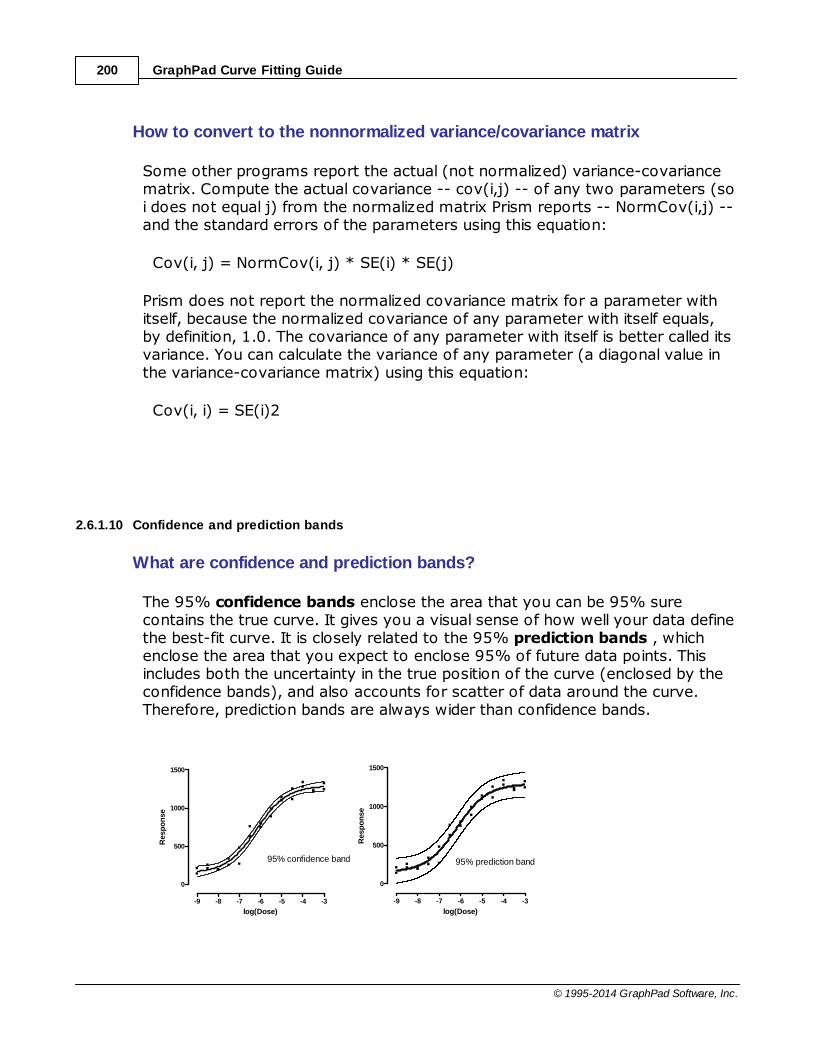
GraphPad Curve Fitting Guide200
© 1995-2014 GraphPad Software, Inc.
How to convert to the nonnormalized variance/covariance matrix
Some other programs report the actual (not normalized) variance-covariancematrix. Compute the actual covariance -- cov(i,j) -- of any two parameters (soi does not equal j) from the normalized matrix Prism reports -- NormCov(i,j) --and the standard errors of the parameters using this equation:
Cov(i, j) = NormCov(i, j) * SE(i) * SE(j)
Prism does not report the normalized covariance matrix for a parameter withitself, because the normalized covariance of any parameter with itself equals,by definition, 1.0. The covariance of any parameter with itself is better called itsvariance. You can calculate the variance of any parameter (a diagonal value inthe variance-covariance matrix) using this equation:
Cov(i, i) = SE(i)2
2.6.1.10 Confidence and prediction bands
What are confidence and prediction bands?
The 95% confidence bands enclose the area that you can be 95% surecontains the true curve. It gives you a visual sense of how well your data definethe best-fit curve. It is closely related to the 95% prediction bands , whichenclose the area that you expect to enclose 95% of future data points. Thisincludes both the uncertainty in the true position of the curve (enclosed by theconfidence bands), and also accounts for scatter of data around the curve.Therefore, prediction bands are always wider than confidence bands.
-9 -8 -7 -6 -5 -4 -3
0
500
1000
1500
log(Dose)
Resp
on
se
95% confidence band
-9 -8 -7 -6 -5 -4 -3
0
500
1000
1500
log(Dose)
Resp
on
se
95% prediction band

CURVE FITTING WITH PRISM 6 201
© 1995-2014 GraphPad Software, Inc.
How to plot confidence bands, prediction bands or both
Choose to plot confidence or prediction bands by an checking option on the Diagnostics tab .
Prism lets you choose either a confidence band or a prediction band, but notboth. To plot both on one graph, you need to analyze your data twice,choosing a confidence band the first time and a prediction band the secondtime.
The regression lines or curves are data sets that you can add to any graph bydrag-n-drop or using the Change menu from the graph.
How to view the XY coordinates of the confidence or prediction bands
Prism can also show you the XY coordinates that define the curve andconfidence bands (or prediction bands). But it only shows this table if you askfor it:
1.Go to the Diagnostics tab and check the option to plot confidence orprediction bands.
2.Go to the Range tab of the nonlinear regression dialog.
3.Check the option to create a table of XY coordinates. This table will includethe confidence or prediction bands.
4.Enter the number of XY pairs you want to define the curve. 150 is areasonable starting value, but of course it all depends on why you want thesevalues.
5.When viewing the results, expand the results sheet in the navigator and go tothe page labeled 'Curve'. For each X value, you'll see the Y value and thedistance the confidence or prediction curve is above and below that value.
How to plot a one-sided confidence or prediction band
In some situations, it makes sense to plot only one side of the confidence orprediction band. One use for a one-sided confidence band would be on a graphthat plots purity of a substance over time. You want to know, with a certainconfidence, how low the purity could be at a certain time. But you don't reallycare about quantifying how high the purity could be.
To plot a one sided 95% confidence or prediction band:
165

GraphPad Curve Fitting Guide202
© 1995-2014 GraphPad Software, Inc.
1.Check the option (on the Diagnostics tab) to plot "90%" confidence (orprediction) bands. When you plot in only one direction, this is really a 95%confidence band.
2. On the Format Graph dialog, choose the data set that defines regressioncurve and make sure that error bars are turned on with the "---" style.
3.Choose to plot those error bands in one direction.
Do not mix up confidence intervals and confidence bands
It is easy to mix up confidence intervals and confidence bands. Choose both onthe Diagnostics tab .
The 95% confidence interval tells you how precisely Prism has found thebest-fit value of a particular parameter. It is a range of values, centered on thebest-fit value. Prism can display this range in two formats:
Don't mix up confidence bands and prediction bands
Note the difference between confidence and prediction bands:
The 95% confidence bands enclose the area that you can be 95% surecontains the true curve. If you have many data points, the confidence bands willbe near the line or curve, and most of your data will lie outside the confidencebands.
The 95% prediction bands enclose the area that you expect to enclose 95% offuture data points. They are wider than confidence bands -- much wider withlarge data sets.
Situations where Prism won't plot confidence or prediction bands
Prism will not plot confidence or prediction bands in several situations:
165

CURVE FITTING WITH PRISM 6 203
© 1995-2014 GraphPad Software, Inc.
If the best-fit value of a parameter hits a constraint , the fit is unlikely to be
useful. Prism does not plot confidence or prediction bands, because theywould almost certainly be misleading.
If the results of nonlinear regression are ambiguous , the confidence or
prediction bands would be super wide, maybe infinitely wide. They would notbe useful, so Prism does not plot them.
If you choose robust nonlinear regression, Prism does not compute
confidence or prediction bands, as it cannot compute standard errors orconfidence intervals of the parameters.
The fit is perfect . If the sum-of-squares is 0.0 and R2 is 1.0, it is not
possible to compute or interpret confidence or prediction bands.
If the fit is interrupted , confidence and prediction bands are not computed.
How are confidence and prediction bands computed?
First, let's define G|x, which is the gradient of the parameters at a particularvalue of X and using all the best-fit values of the parameters. The result is avector, with one element per parameter. For each parameter, it is defined asdY/dP, where Y is the Y value of the curve given the particular value of X and allthe best-fit parameter values, and P is one of the parameters.)
G'|x is that gradient vector transposed, so it is a column rather than a row ofvalues.
Cov is the covariance matrix (inversed Hessian from last iteration). It is asquare matrix with the number of rows and columns equal to the number ofparameters. Each item in the matrix is the covariance between twoparameters. We use Cov to refer to the normalized covariance matrix, whereeach value is between -1 and 1. Details and comparison to nonnormalizedcovariance matrix.
Now compute c = G'|x * Cov * G|x. The result is a single number for any valueof X.
The confidence and prediction bands are centered on the best fit curve, andextend above and below the curve an equal amount.
The confidence bands extend above and below the curve by:
= sqrt(c)*sqrt(SS/DF)*CriticalT(Confidence%, DF)
231
228
233
226

GraphPad Curve Fitting Guide204
© 1995-2014 GraphPad Software, Inc.
The prediction bands extend a further distance above and below the curve,equal to:
= sqrt(c+1)*sqrt(SS/DF)*CriticalT(Confidence%, DF)
In both these equations, the value of c (defined above) depends on the value ofX, so the confidence and prediction bands are not a constant distance from thecurve. The value of SS is the sum-of-squares for the fit, and DF is the numberof degrees of freedom (number of data points minus number of parameters).CriticalT is a constant from the t distribution based on the amount of confidenceyou want and the number of degrees of freedom. For 95% limits, and a fairlylarge df, this value is close to 1.96. If DF is small, this value is higher.
Read a more mathematical explanation.
2.6.1.11 Hougaard's measure of skewness
Consequences of an asymmetrical parameter
Even though nonlinear regression, as its name implies, is designed to fit nonlinearmodels, some of the inferences actually assume that some aspects of the modelare close to linear, so that the uncertainty about each parameter's value issymmetrical. This means that if you analyzed many data sets sampled from thesame system, the distribution of the best-fit values of the parameter would besymmetrical and Gaussian.
If the distribution of a parameter is highly skewed, there are two consequences:
The SE of that parameter will not be a very useful measure of uncertainty. The
SE is interpreted as a plus-minus assessment of how sure you are of theparameter value. But if the parameter is very asymmetrical, then a single SEcannot really describe the uncertainty.
The confidence interval for that parameter cannot be interpreted at face value.
Prism always computes the CI from the SE of that parameter (and the numberof degrees of freedom), and the CI is always symmetrical around the best-fitvalue. If the parameter is very asymmetrical, then that symmetrical confidenceinterval does not give a accurate picture of the uncertainty.
429

CURVE FITTING WITH PRISM 6 205
© 1995-2014 GraphPad Software, Inc.
Hougaard's measure of skewness
Hougaard (1) developed a way to assess the skewness of a parameter used innonlinear regression without doing any simulations. Prism will compute thisvalue for each parameter when you check the option the Diagnostics tab ofnonlinear regression in the section labeled "Are the parameters intertwined,redundant or skewed?". The results are tabulated along with the other resultsof nonlinear regression.
Ratkowsky has proposed the following interpretation:
Absolute value Interpretation
<0.10Ideal. Almost linear. Confidence intervals can be interpretedat face value
0.10 - 0.25 Adequate
0.25 - 1.00Noticeable skewness. Consider alternative parameterizationsof the equation
> 1.00 Considerable skewness. Strongly consider alternatives
Note that these values are for the absolute value of the Hougaard's measure.
For the simulated data set for the example above, Hougaard's skewness is0.09 for Khalf and 1.83 for Kprime. This one value (no simulations needed) tellsyou to choose the form of the model that fits Khalf rather than the form thatfits Kprime.
Notes
Hougaard's measure of skewness is measured for each parameter in the
equation (omitting parameters fixed to constant values).
Prism does not compute Hougaard's skewness if you chose unequal
weighting, or a robust fit, because the method is not defined for thesesituations.
The values depend on the equation, the number of data points, the spacing of
the X values, and the values of the parameters.
Hougaard's measure of skewness has no units.

GraphPad Curve Fitting Guide206
© 1995-2014 GraphPad Software, Inc.
The SAS documentation does a great job of explaining Hougaard's measure
(3).
References
1. P. Hougaard. The appropriateness of the asymptotic distribution in anonlinear regression model in relation to curvature. Journal of the RoyalStatistical Society. Series B (Methodological) (1985) pp. 103-114
2. David A. Ratkowsky, Nonlinear Regression Modeling: A Unified PracticalApproach (Statistics: a Series of Textbooks and Monogrphs).IBSN:0824719077
3.SAS documentation about Hougaard's measure.
2.6.1.12 Could the fit be a local minimum?
What is a false minimum?
The nonlinear regression procedure adjusts the variables in small steps in orderto improve the goodness-of-fit. If Prism converges on an answer, you can besure that altering any of the variables a little bit will make the fit worse. But it istheoretically possible that large changes in the variables might lead to a muchbetter goodness-of-fit. Thus the curve that Prism decides is the "best" mayreally not be the best.
Think of latitude and longitude as representing two variables Prism is trying tofit. Now think of altitude as the sum-of-squares. Nonlinear regression worksiteratively to reduce the sum-of-squares. This is like walking downhill to find thebottom of the valley. When nonlinear regression has converged, changing anyvariable increases the sum-of-squares. When you are at the bottom of thevalley, every direction leads uphill. But there may be a much deeper valley over

CURVE FITTING WITH PRISM 6 207
© 1995-2014 GraphPad Software, Inc.
the ridge that you are unaware of. In nonlinear regression, large changes invariables might decrease the sum-of-squares.
This problem (called finding a local minimum) is intrinsic to nonlinear regression,no matter what program you use. You will rarely encounter a local minimum ifyour data have little scatter, you collected data over an appropriate range of Xvalues, and you have chosen an appropriate equation.
Testing for a false minimum
To test for the presence of a false minimum:
1.Note the values of the variables and the sum-of-squares from the first fit.
2.Make a large change to the initial values of one or more parameters andrun the fit again.
3.Repeat step 2 several times.
Ideally, Prism will report nearly the same sum-of-squares and same parametersregardless of the initial values. If the values are different, accept the ones withthe lowest sum-of-squares.
2.6.1.13 Outliers
The outliers table
If you choose to exclude or count outliers as part of nonlinear regression, oneof the results tables will list all outliers.
Keep in mind an important distinction:
If you chose to count outliers (on the Diagnostics tab ), then the outliers
are still included in the fit.
If you chose to exclude outliers (on the Fit tab ), then the outliers are
ignored by the fit, but are still included on the graph .
In both cases, the aggressiveness of the outlier hunt is determined by the ROUT
165
155
176

GraphPad Curve Fitting Guide208
© 1995-2014 GraphPad Software, Inc.
coefficient Q that you enter on the Weights tab .
What does it mean to be an outlier
Prism uses the ROUT algorithm , using the value of Q that you can adjust inthe Weights tab , to decide when to declare a point to be an outlier. Someconsiderations:
The first thing to do is make sure it isn't simply a problem in data entry. If
so, fix it.
Review the list of situations where the outlier identification procedure should
not be used .
Be alert to biological variation. In some experimental situations, outliers can
only arise from lab mistakes. These should be excluded. In other situations,an outlier can be the result of biological variation. You may have discovereda new polymorphism in some gene. It could be missing a big opportunity ifyou exclude and ignore those values.
What to do once you have identified an outlier
After you have identified one or more outliers, you have several choices.
While outliers are ignored by the nonlinear regression calculation, they are
still plotted on the graph. If you want the outlier to be entirely removedfrom the graph, including error bars on the graph, go back to the data tableand exclude the outlier(s). Prism will then refit the curve, and replot thegraph without any outliers.
If you want the outlier to remain on the graph, simply polish the graph Prism
provides. Keep in mind that the outliers are a dataset, so you canseparately adjust the size, color and symbol of outliers and all the datapoints. Use the "Datasets on graph" tab of Format Graph to adjust theback-to-front order of data sets to keep the outlier in front of the otherdata sets. The dialog shows the datasets in back to front order, so youwant to keep the outlier data sets lower in the list.
If you want to remove the special formatting of outliers on the graph, use
the "Datasets on graph" tab of Format Graph. Select the outlier dataset(s)and click Remove. The outlier will still be plotted as part of the full data set,but will no longer be plotted separately as an outlier data set.
If you asked Prism to count the outliers (Diagnostics tab) but now wish to
160
53
160
54

CURVE FITTING WITH PRISM 6 209
© 1995-2014 GraphPad Software, Inc.
fit the data with the outlier ignored, go back to the nonlinear regressiondialog and choose "Automatic outlier elimination" (on the Fit tab).
2.6.1.14 Troubleshooting nonlinear regression
The #1 tip for troubleshooting
Nonlinear regression starts with initial values for each parameter. If these initialvalues are very far from the correct values, nonlinear regression might goastray. To check this, go to theDiagnostics tab of the nonlinear regressiondialog and choose the option at the top of the dialog: Don't fit a curve.Instead plot the curve defined by the initial values of the parameters.
If the curve defined by the initial values does not generally follow the shape ofthe data, and go near the data points, you should change the initial values(Initial Values tab of nonlinear regression ) until they do.
If Prism reports an error code
Prism reports error codes as a single phrase that appears over the column ofresults, for example "Bad initial values" or "Impossible weights". Learn moreabout each error message.
Common problems in nonlinear regression
Here is a short list of potential curve fitting problems with suggested solutions.
The equation simply does not describe the data.
Try a different equation.
The initial values are too far from their correct values.
Enter different initial (estimated) values for the parameters. If you entered yourown equation, check that you entered sensible rules for generating initialvalues.
The range of X values is too narrow to define the curve completely.
If possible, collect more data. Otherwise, hold one of the parameters to aconstant value.
165
162
225

GraphPad Curve Fitting Guide210
© 1995-2014 GraphPad Software, Inc.
You have not collected enough data in a critical range of X values.
Collect more data in the important regions.
Your data are very scattered and don't really define a curve.
Try to collect less scattered data. If you are combining several experiments,consider normalizing the data for each experiment to an internal control.
The equation includes more than one component, but your data don't follow amulticomponent model.
Use a simpler equation.
Your numbers are too large or too small.
If your X or Y values are huge, divide by a constant to change the units. Avoidvalues greater than, say, 100,000.
If your X or Y values are tiny, multiply by a constant change the units. Avoidvalues less than about 0.00001.
Changing the units is unlikely to solve the problem, but it is worth a try.
You've set a parameter to an inappropriate constant value.
Check that you haven't made a simple mistake like setting a maximum plateauto 1.0 when it should be 100, or a Hill slope to +1.0 when it should be -1.0.
Consult an analysis check list
Prism has three different analysis checklists for nonlinear regression. Use theone that matches your goal.
Analysis checklist: Fitting a model
Analysis checklist: Comparing nonlinear fits
Analysis checklist: Interpolating from a standard curve
218
221
223
CURVE FITTING WITH PRISM 6 211
© 1995-2014 GraphPad Software, Inc.
2.6.1.15 Why results in Prism 5 and 6 can differ from Prism 4
Prism 5 and 6 use the same algorithms, so should always report identicalresults.
However, Prism 4 used slightly different algorithms, so curve fitting results candiffer from results with Prism 5 or 6 in these cases:
If your fit is labeled "Ambiguous" by Prism 5 or 6, you know that some of the
parameters are not determined precisely. Prism 4 presented a full set ofresults in this case, but the results are not useful when the fit is ambiguous.
If you chose no weighting, check the sum-of-squares from the two
programs. The goal of regression is to minimize that sum of squares, so seewhich version of Prism found a fit with the smaller sum-of-squares. Prism 5and 6 have a few improvements in the fitting algorithm, so occasionally it canfind a better fit than did Prism 4. The differences, if any, are usually trivial.
If you chose to weight by the Y values (or the Y values squared), Prism 5 and
6 handle weighting differently than did Prism 4. Prism now weights by the Yvalue of the curve, while Prism 4 (and earlier releases) weighted by the Yvalue of the data. Weighting by the Y value of the curve is better, so theresults of Prism 5 and 6 are more correct. Since the weighting is computeddifferently, you can't directly compare the weighted sum-of-square valuesreported by the two versions of Prism.
When you compare two models, Prism now does an extra step. If one of the
models is ambiguous, then Prism chooses the other model, without doing theF test or AIC comparison.
Prism now offers more rules for defining initial parameter values. If your
equation uses one of these new rules, Prism 4 might not be able to find areasonable fit until you tweak those initial values. In particular, Prism now hassmarter rules for fitting sigmoidal log(dose) vs. response curves.
If you entered data as mean, SD (or SEM) and N, then Prism 4 (by default)
fits the means and weights by the sample size (N). This is one of the twooptions on the weighting tab (the other option is to fit means only, ignoringN). Prism is now smarter by default (although you can choose to just fit themeans and ignore N and SD values). It accounts not only for sample size Nbut also for the SD (or SEM) values you enter. With Prism 5 or 6 (but notPrism 4), you'll get exactly the same results from data entered as mean, SDand N as you would have by entering raw data. Prism 4 only accounts fordifferences in N, but not SD. The best fit values of the parameters, and thusthe appearance of the curve, is the same with Prism 4 and 5. But Prism 5

GraphPad Curve Fitting Guide212
© 1995-2014 GraphPad Software, Inc.
does a smarter job with standard errors, confidence intervals, andcomparisons of models.
2.6.2 Interpreting results: Comparing models
In many cases, your primary goal in fitting curves is to comparemodels, or compare fits of two (or more) data sets.
First review the general principles ofcomparing models.
Next review the method you choose to use: Extra sum-of-squares or AIC modelcomparison .
Review how Prism compares models when itdetects outliers .
2.6.2.1 Interpreting comparison of models
Reality check before statistics
Apply a common sense reality check before looking at any statistical approachto comparing fits. If one of the fits has results that are scientifically invalid, thenaccept the other model. Only when both fits make scientific sense should youuse statistical method to compare the two fits .
Prism partially automates this 'reality check' approach. If the fit of either modelis ambiguous , then Prism chooses the other model without performing anystatistical test.
Statistical approaches balance the change in sum-of-squares with thechange in numbers of degrees of freedom
The more complicated model (the one with more parameters) almost alwaysfits the data better than the simpler model. Statistical methods are needed tosee if this difference is enough to prefer the more complicated model. Prism cando this via the extra sum-of-squares F test or using information theory andcomputation of AIC .
Both these methods only make sense when the models being compared havedifferent numbers of parameters, and so have different numbers of degrees of
212
213
215
215
228
213
215

CURVE FITTING WITH PRISM 6 213
© 1995-2014 GraphPad Software, Inc.
freedom. If you want to compare two models with the same number ofparameters, there is no need to use either the F test or AIC. Simply choose themodel that fits the data the best with the smallest sum-of-squares.
How do these methods work to compare data sets?
The Compare tab of Prism lets you ask "Do the best-fit values of selectedunshared parameters differ between data sets?" or "Does one curveadequately fit all data sets?". Applying the F test or Akaike's method toanswering these questions is straightforward. Prism compares the sum-of-squares of two fits.
In one fit, the model is separately fit to each data set, and the goodness-of-fit
is quantified with a sum-of-squares. The sum of these sum-of-square valuesquantifies the goodness of fit of the family of curves fit to all the data sets.
The other fit is a global fit to all the data sets at once, sharing specified
parameters. If you ask Prism whether one curve adequately fits all data sets,then it shares all the parameters.
These two fits are nested (the second is a simpler case of the first, with fewerparameters to fit) so the sums-of-squares (actually the sum of sum of squaresfor the first fits) can be compared using either the F test or Akaike's method
.
2.6.2.2 Interpreting the extra sum-of-squares F test
The extra-sum-of-squares F test compares nested models
The extra-sum-of-squares F test compares the goodness-of-fit of twoalternative nested models. "Nested" means that one model is a simpler case ofthe other. Let's consider what this means in different contexts:
If you asked Prism to test whether parameters are different between
treatments, then the models are nested. You are comparing a model wherePrism finds separate best-fit values for some parameters vs. a model wherethose parameters are shared among data sets. The second case (sharing) isa simpler version (fewer parameters) than the first case (individualparameters).
If you asked Prism to test whether a parameter value is different than a
hypothetical value, then the models are nested. You are comparing the fit of a
157
213
215

GraphPad Curve Fitting Guide214
© 1995-2014 GraphPad Software, Inc.
model where a parameter is fixed to a hypothetical value to the fit of a modelwhere Prism finds the best-fit value of that parameter. The first case (fixedvalue) is a simpler version (fewer parameters to fit) than the second.
if you are comparing the fits of two equations you chose, and both models
have the same number of parameters, then the two models cannot benested. With nest models, one model has fewer parameters than the other.When the two models have the same number of parameters, Prism reportsthat it cannot compute the F test because the two models have the samenumber of degrees of freedom. In this case, Prism does not report a P value,and chooses to plot the model whose fit has the lower sum-of-squares. Prismreports the error message, "Models have the same DF."
if you are comparing the fits of two equations you chose with different
numbers of parameters, the models may or may not be nested. Prism doesnot attempt to do the algebra necessary to make this determination. If youchose two models that are not nested, Prism will report results for the extra-sum-of-squares F test, and these results will not be useful.
Interpreting the P value
The extra-sum-of-squares F test is based on traditional statistical hypothesistesting. The F test compares the improvement of SS with the morecomplicated model vs. the loss of degrees of freedom.
The null hypothesis is that the simpler model (the one with fewer parameters)is correct. The improvement of the more complicated model is quantified as thedifference in sum-of-squares. You expect some improvement just by chance,and the amount you expect by chance is determined by the number of degreesof freedom in each model. The F test compares the difference in sum-of-squares with the difference you’d expect by chance. The result is expressed asthe F ratio, from which a P value is calculated.
The P value answers this question:
If the null hypothesis is really correct, in what fraction of experiments (thesize of yours) will the difference in sum-of-squares be as large as youobserved, or even larger?
If the P value is small, conclude that the simple model (the null hypothesis) iswrong, and accept the more complicated model. Usually the threshold P valueis set at its traditional value of 0.05.
If the P value is high, conclude that the data do not present a compelling reasonto reject the simpler model.

CURVE FITTING WITH PRISM 6 215
© 1995-2014 GraphPad Software, Inc.
Prism names the null and alternative hypotheses, and reports the P value. Youset the threshold P value in the Compare tab of the nonlinear regression dialog.If the P value is less than that threshold, Prism chooses (and plots) thealternative (more complicated) model. It also reports the value of F and thenumbers of degrees of freedom, but these will be useful only if you want tocompare Prism's results with those of another program or hand calculations.
2.6.2.3 Interpreting AIC model comparison
This alternative approach is based on information theory, and does not use thetraditional “hypothesis testing” statistical paradigm. Therefore it does notgenerate a P value, does not reach conclusions about “statistical significance”,and does not “reject” any model.
The method determines how well the data supports each model, taking intoaccount both the goodness-of-fit (sum-of-squares) and the number ofparameters in the model. The results are expressed as the probability that eachmodel is correct, with the probabilities summing to 100%. If one model is muchmore likely to be correct than the other (say, 1% vs. 99%), you will want tochoose it. If the difference in likelihood is not very big (say, 40% vs. 60%), youwill know that either model might be correct, so will want to collect more data.
Of course, these probabilities are meaningful only in the context of comparingthose two models. It is possible a third model you didn't test fits much betterso is much more likely to be correct.
Prism names the null and alternative hypotheses, and reports the likelihood thateach is correct It also reports the difference between the AICc values (as theAICc of the simple model minus the AICc of the more complicated model), butthis will be useful only if you want to compare Prism's results with those ofanother program or hand calculations. Prism chooses and plots the model thatis more likely to be correct, even if the difference in likelihoods is small.
2.6.2.4 How Prism compares models when outliers are eliminated
Comparing models only makes sense when both models 'see' exactly the sameset of data. That makes it tricky to combine outlier elimination with model

GraphPad Curve Fitting Guide216
© 1995-2014 GraphPad Software, Inc.
comparison. Prism handles this situation automatically.
If you select automatic outlier elimination (on the Fit tab ), Prism first fitseach model separately to determine which points (if any) are outliers. Then itremoves all the points that are defined as outliers from either of the models,and fits both models again. It uses the sum-of-squares and df from these fits toperform the comparison. This approach ensures that exactly the same pointsare fit to both models, and that outliers from either model are excluded.
2.6.2.5 Interpreting the adjusted R2
Why you should not use R2 to compare models
R2 quantifies how well a model fits the data, so it seems as though it would bean easy way to compare models. It sure sounds easy -- pick the model withthe larger R2. The problem with this approach is that there is no penalty foradding more parameters. So the model with more parameters will bend andtwist more to come nearer the points, and so almost always has a higher R2. Ifyou use R2 as the criteria for picking the best model, you'd almost always pickthe model with the most parameters.
The adjusted R2 accounts for the number of parameters fit
The adjusted R2 always has a lower value than R2 (unless you are fitting onlyone parameter). The equations below show why.
The equations above show how the adjusted R2 is computed. The sum-of-squares of the residuals from the regression line or curve have n-K degrees offreedom, where n is the number of data points and K is the number ofparameters fit by the regression. The total sum-of-squares is the sum of thesquares of the distances from a horizontal line through the mean of all Y values.Since it only has one parameter (the mean), the degrees of freedom equals n-
155
CURVE FITTING WITH PRISM 6 217
© 1995-2014 GraphPad Software, Inc.
1. The adjusted R2 is larger than the ordinary R2 whenever K is greater than 1.
Using adjusted R2 and a quick and dirty way to compare models
A quick and easy way to compare models is to choose the one with the smalleradjusted R2. Choose to report this value on the Diagnostics tab .
Comparing models with adjusted R2 is not a standard method for comparingnonlinear models (it is standard for multiple linear regression), and we suggestthat you use the extra-sum-of-square F test or comparing AICc instead. Ifyou do compare models by comparing adjusted R2, make sure that identicaldata, weighted identically, are used for all fits.
Adjusted R2 in linear regression
Prism doesn't report the adjusted R2 with linear regression, but you can fit astraight line with nonlinear regression.
If X and Y are not linearly related at all, the best fit slope is expected to be 0.0.If you analyzed many randomly selected samples, half the samples would havea slope that is positive and half the samples would have a negative slope. Butin all these cases, R2 would be positive (or zero). R2 can never be negative(unless you constrain the slope or intercept so it is forced to fit worse than ahorizontal line). In contrast, the adjusted R2 can be negative. If you analyzedmany randomly selected samples, you'd expect the adjusted R2 to be positivein half the samples and negative in the other half.
Here is a simple way to think about the distinction. The R2 quantifies the linearrelationship in the sample of data you are analyzing. Even if there is nounderlying relationship, there almost certainly is some relationship in thatsample. The adjusted R2 is smaller than R2 and is your best estimate of thedegree of relationship in the underlying population.
2.6.3 Analysis checklists: Nonlinear regression
To understand your results, review the appropriate analysischecklist, depending on your experimental goal.
Analysis checklist: Fitting a model
Analysis checklist: Comparing nonlinear fits
Analysis checklist: Interpolating from astandard curve
165
213 215
218
221
223

GraphPad Curve Fitting Guide218
© 1995-2014 GraphPad Software, Inc.
2.6.3.1 Analysis checklist: Fitting a model
Your approach in evaluating nonlinear regression depends on your goal.
In many cases, your goal is to create a standard curve from which tointerpolate unknown values. We've created a different checklist for thispurpose.
More often, your goal is to determine the best-fit values of the model. If that isyour goal, here are some questions to ask yourself as you evaluate the fit:
Curve
Does the graph look sensible?
Your first step should be to inspect a graph of the data with superimposedcurve. Most problems can be spotted that way.
Does the runs or replicate test tell you that the curve deviatessystematically from the data?
The runs and replicates tests are used to determine whether the curvefollows the trend of your data. The runs test is used when you have single Yvalues at each X. It asks if data points are clustered on either side of the curverather than being randomly scattered above and below the curve. Thereplicates test is used when you have replicate Y values at each X. It asks if thepoints are 'too far' from the curve compared to the scatter among replicates.
If either the runs test or the replicates test yields a low P value, you canconclude that the curve doesn't really describe the data very well. You mayhave picked the wrong model, or applied invalid constraints.
Parameters
Are the best-fit parameter values plausible?
When evaluating the parameter values reported by nonlinear regression, check
223
193 194

CURVE FITTING WITH PRISM 6 219
© 1995-2014 GraphPad Software, Inc.
that the results are scientifically plausible. Prism doesn't 'know' what theparameters mean, so can report best-fit values of the parameters that makeno scientific sense. For example, make sure that parameters don't haveimpossible values (rate constants simply cannot be negative). Check that EC50values are within the range of your data. Check that maximum plateaus aren'ttoo much higher than your highest data point.
If the best-fit values are not scientifically sensible, then the results won't beuseful. Consider constraining the parameters to a sensible range, and tryingagain.
How precise are the best-fit parameter values?
You don't just want to know what the best-fit value is for each parameter. Youalso want to know how certain that value is. Therefore an essential part ofevaluating results from nonlinear regression is to inspect the 95% confidenceintervals for each parameter.
If all the assumptions of nonlinear regression are true, there is a 95% chancethat the interval contains the true value of the parameter. If the confidenceinterval is reasonably narrow, you've accomplished what you wanted to do –found the best fit value of the parameter with reasonable certainty. If theconfidence interval is really wide, then you've got a problem. The parametercould have a wide range of values. You haven't nailed it down. How wide is 'toowide' depends on the scientific context of your work.
Are the confidence bands 'too wide'?
Confidence bands visually show you how precisely the parameters have beendetermined. Choose to plot confidence bands by checking an option on the Fittab of the nonlinear regression dialog. If all the assumptions of nonlinearregression have been met, then there is a 95% chance that the true curve fallsbetween these bands. This gives you a visual sense of how well your datadefine the model.
Residuals
Does the residual plot look good?
A residual plot shows the relationship between the X values of your data andthe distance of the point from the curve (the residuals). If the assumptions ofthe regression are met, the residual plot should look bland, with no trendsapparent.
179

GraphPad Curve Fitting Guide220
© 1995-2014 GraphPad Software, Inc.
Does the scatter of points around the best-fit curve follow a Gaussiandistribution?
Least squares regression is based on the assumption that the scatter of pointsaround the curve follows a Gaussian distribution. Prism offers three normalitytests (in the Diagnostics tab) that can test this assumption (we recommend theD'Agostino test). If the P value for a normality test is low, you conclude thatthe scatter is not Gaussian.
Could outliers be impacting your results?
The presence of one or a few outliers (points much further from the curve thanthe rest) can overwhelm the least-squares calculations and lead to misleadingresults.
You can spot outliers by examining a graph (so long as you plot individualreplicates, and not mean and error bar). But outliers can also be detectedautomatically. GraphPad has developed a new method for identifying outlierswe call the ROUT method. Check the option on the diagnostics tab to count theoutliers, but leave them in the calculations. Or check the option on the Fit tab toexclude outliers from the calculations.
Models
Would another model be more appropriate?
Nonlinear regression finds parameters that make a model fit the data as closelyas possible (given some assumptions). It does not automatically ask whetheranother model might work better.
Even though a model fits your data well, it may not be the best, or mostcorrect, model. You should always be alert to the possibility that a differentmodel might work better. In some cases, you can't distinguish between modelswithout collecting data over a wider range of X. In other cases, you would needto collect data under different experimental conditions. This is how sciencemoves forward. You consider alternative explanations (models) for your data,and then design experiments to distinguish between them.
If you chose to share parameters among data sets, are thosedatasets expressed in the same units?
Global nonlinear regression (any fit where one or more parameter is sharedamong data sets) minimizes the sum (over all datasets) of the sum (over all

CURVE FITTING WITH PRISM 6 221
© 1995-2014 GraphPad Software, Inc.
data points) of the squared distance between data point and curve. This onlymakes sense if the Y values for all the datasets are expressed in the sameunits.
Goodness of fit
Is the R2 'too low' compared to prior runs of this experiment?
While many people look at R2 first, it really doesn't help you understand theresults very well. It only helps if you are repeating an experiment you have runmany times before. If so, then you know what value of R2 to expect. If the R2
is much lower than expected, something went wrong. One possibility is thepresence of outliers.
Are the values of sum-of-squares and sy.x 'too low' compared toprior runs of this experiment?
These values are related to the R2, and inspecting the results can only be usefulwhen you have done similar experiments in the past so know what values toexpect.
2.6.3.2 Analysis checklist: Comparing nonlinear fits
Approach to comparing models
Which model is 'best'? At first, the answer seems simple. The goal of nonlinearregression is to minimize the sum-of-squares, so the model with the smallersum-of-squares clearly fits best. But that is too simple.
The model with fewer parameters almost always fits the data worse. When youcompare two models, the simpler model (with fewer parameters) will have ahigher sum-of-squares. When you compare datasets, the global fit will have ahigher sum-of-squares than the sum of the individual fits. And when youcompare fits with and without a parameter constrained to a particular value, willhave a higher sum-of-squares than a model where you don't constrain theparameter.
Both the F test and the AIC method take into account both the difference ingoodness-of-fit but also the number of parameters. The question is whetherthe decrease in sum of squares (moving from simpler to more complicatedmodel) is worth the 'cost' of having more parameters to fit. The F test and

GraphPad Curve Fitting Guide222
© 1995-2014 GraphPad Software, Inc.
AICc methods approach this question differently.
How Prism reports model comparison
Prism reports the results for the comparison at the top of the nonlinearregression table of results. It clearly states the null and alternative hypotheses.If you chose the F test, it reports the F ratio and P value. If you chose Akaike'smethod, it reports the difference in AICc and the probability that each model iscorrect.
Finally, Prism reports the 'preferred' model. You should understand how Prismdecides which model is 'preferred' as you may 'prefer' the other model.
If you chose the extra sum-of-squares F test, then Prism computes a P valuethat answers this question:
If the null hypothesis is really correct, in what fraction of experiments (thesize of yours) will the difference in sum-of-squares be as large as youobserved or larger?
In the Compare tab, you also tell Prism which P value to use as the cut off (thedefault is 0.05). If the P value is lower than that value, Prism chooses the morecomplicated model. Otherwise it chooses the simpler model.
If you chose Akaike's method, Prism chooses the model that is more likely tobe correct. But you should look at the two probabilities. If they are similar invalue, then the evidence is not persuasive and both models fit pretty well.
Analysis checklist for comparing models
Was it possible to fit both models?
Before running the extra sum-of-squares F test or computing AICc values,Prism first does some common sense comparisons. If Prism is unable to fit
48

CURVE FITTING WITH PRISM 6 223
© 1995-2014 GraphPad Software, Inc.
either model, or if either fit is ambiguous or perfect , then Prism does notcompare models.
Are both fits sensible?
Apply a reality check before accepting Prism's results. If one of the fits hasresults that are scientifically invalid, then accept the other model regardless ofthe results of the F test or AIC comparison.
For example, you would not want to accept a two-phase exponential model ifthe magnitude of one of the phases is only a tiny fraction of the total response(especially if you don't have many data points). And you wouldn't want toaccept a model if the half-life of one of the phases has a value much less thanyour first time point or far beyond your last time point.
Analysis checklist for the preferred model
Before accepting the 'preferred' model, you should think about the same set ofquestions as you would when only fitting one model. You can consult the detailed checklist or the abbreviated version below.
How precise are the best-fit parameter values?
Are the confidence bands 'too wide'?
Does the residual plot look good?
Does the scatter of points around the best-fit curve follow a Gaussiandistribution?
2.6.3.3 Analysis checklist: Interpolating from a standard curve
Your approach in evaluating nonlinear regression depends on your goal.
In many cases, your goal is to learn from the best-fit values. If that is yourgoal, view a different checklist .
If your goal is to create a standard curve from which to interpolate unknownvalues, your approach depends on whether this is a new or established assay.
228 233
218
218
GraphPad Curve Fitting Guide224
© 1995-2014 GraphPad Software, Inc.
Established assay
If the assay is well established, then you know you are fitting the right modeland know what kind of results to expect. In this case, evaluating a fit is prettyeasy.
Does the curve go near the points?
Is the R2 'too low' compared to prior runs of this assay?
If so, look for outliers, or use Prism's automatic outlier detection.
Are the confidence bands too wide?
The confidence bands let you see how accurate interpolations will be, so wesuggest always plotting prediction bands when your goal is to interpolate fromthe curve. If your are running an established assay, you know how wide youexpect the prediction bands to be.
New assay
With a new assay, you also have to wonder about whether you picked anappropriate model.
Does the curve go near the points?
Look at the graph. Does it look like the curve goes near the points.
Are the prediction bands too wide?
How wide is too wide? The prediction bands show you how preciseinterpolations will be. Draw a horizontal line somewhere along the curve, andlook at the two places where that line intercepts the prediction bands. This willbe the confidence interval for the interpolation.
Does the scatter of points around the best-fit curve follow a Gaussiandistribution?
Least squares regression is based on the assumption that the scatter of pointsaround the curve follows a Gaussian distribution. Prism offers three normalitytests (in the Diagnostics tab) that can test this assumption (we recommend theD'Agostino test). If the P value for a normality test is low, you conclude that
171

CURVE FITTING WITH PRISM 6 225
© 1995-2014 GraphPad Software, Inc.
the scatter is not Gaussian.
Could outliers be impacting your results?
Nonlinear regression is based on the assumption that the scatter of dataaround the ideal curve follows a Gaussian distribution. This assumption leads tothe goal of minimizing the sum of squares of distances of the curve from thepoints. The presence of one or a few outliers (points much further from thecurve than the rest) can overwhelm the least-squares calculations and lead tomisleading results.
You can spot outliers by examining a graph (so long as you plot individualreplicates, and not mean and error bar). But outliers can also be detectedautomatically. GraphPad has developed a new method for identifying outlierswe call the ROUT method. check the option on the diagnostics tab to count theoutliers, but leave them in the calculations. Or check the option on the Fit tab toexclude outliers from the calculations.
Does the curve deviate systematically from the data?
If either the runs test or the replicates test yields a low P value, then you canconclude that the curve doesn't really describe the data very well. You mayhave picked the wrong model.
2.6.4 Error messages from nonlinear regression
When Prism hits a problem, it will present a verybrief message in the top row of the resultstables. Read the pages in this section to learnwhat these messages mean.
"Bad initial values"
"Interrupted"
"Not converged"
"Ambiguous"
"Hit constraint"
"Don't fit"
226
226
227
228
231
232

GraphPad Curve Fitting Guide226
© 1995-2014 GraphPad Software, Inc.
"Too few points"
"Perfect fit"
"Impossible weights"
"Equation not defined"
2.6.4.1 "Bad initial values"
What does "bad initial values" mean?
Nonlinear regression works iteratively. Prism starts with initial estimated valuesfor each parameter. It then gradually adjusts these until it converges on thebest fit. In rare circumstances, Prism cannot compute a curve based on theinitial values you entered. When it tries, it encounters a math problem such asdivision by zero or taking the logarithm of a negative number. In this case,Prism does not report any results and instead reports "bad initial values".
Checklist
Did you enter or choose the right equation?
Did you enter sensible values for initial values?
Is the range of X values invalid? Focus on the first and last X value (and onX=0 if included in the range). Can the equation be evaluated at those X valueswith the initial values you entered?
2.6.4.2 "Interrupted"
What does 'interrupted' mean?
Prism reports 'interrupted' in two situations:
Nonlinear regression takes more iterations than the maximum entered on
the diagnostics tab (the default is 1000).
The fit was slow, and you clicked "Interrupt" on the progress dialog.
Checklist
If the maximum number of iterations was set to a low value, set it to a higher
232
233
233
233

CURVE FITTING WITH PRISM 6 227
© 1995-2014 GraphPad Software, Inc.
value and try again. If you have lots of data points and lots of parameters,nonlinear regression can sometimes require hundreds of iterations.
If the maximum number of iterations was already set to a high value, you cantry a still higher value, but most likely Prism is still not going to be able to find abest-fit curve. Things to check:
Did you enter the right model?
Does the curve defined by your initial values come near your data? Checkthe option on the diagnostics tab to plot that curve.
If you entered constraints, were they entered correctly?
If you didn't enter any constraints, consider whether you can constrainone or more parameters to a constant value? For example, in a dose-response curve can you constrain the bottom plateau to be zero?
Can you share a parameter over all the data sets (global fitting)?
2.6.4.3 "Not converged"
What does "not converged" mean?
Nonlinear regression works iteratively. Prism starts with initial estimated valuesfor each parameter. It then gradually adjusts these until it converges on thebest fit. "Converged" means that any small change in parameter values createsa curve that fits worse (higher sum-of-squares). But in some cases, it simplycan't converge on a best fit, and gives up with the message 'not converged'.This happens in two situations:
The model simply doesn't fit the data very well. Perhaps you picked the
wrong model, or applied the wrong constraints.
The initial values generated a curve that didn't come close to the points. In
that case, Prism may not be able to figure out how to change theparameters to make the curve fit well.
Checklist
Did you enter the right model?
165

GraphPad Curve Fitting Guide228
© 1995-2014 GraphPad Software, Inc.
Does the curve defined by your initial values come near your data? Checkthe option on the diagnostics tab to plot that curve.
If you entered constraints, were they entered correctly?
If you didn't enter any constraints, consider whether you can constrainone or more parameters to a constant value? For example, in a dose-response curve can you constrain the bottom plateau to be zero?
Can you share a parameter over all the data sets (global fitting)?
2.6.4.4 "Ambiguous"
What does "ambiguous" mean?
"Ambiguous" is a term coined by GraphPad to describe a fit that doesn't reallynail down the values of all the parameters.
Changing the value of any parameter will always move the curve further fromthe data and increase the sum-of-squares. But when the fit is 'ambiguous',changing other parameters can move the curve so it is near the data again. Inother words, many combinations of parameter values lead to curves that fitequally well.
Prism puts the word 'ambiguous' in the top row of results. For the parametersthat are 'ambiguous' (there may be one or several), Prism puts '~' before thebest fit values and standard errors, and reports "very wide" for thecorresponding confidence intervals.
If you check the option in the diagnostics tab to report dependency, the valuewill be >0.9999 for all the 'ambiguous' parameters (that is how we define'ambiguous'; the threshold value is arbitrary).
If the fit is 'ambiguous' you really can't interpret the best-fit values of someparameters.
Does it matter?
If your goal is to interpolate unknowns from a standard curve, you won't carethat the parameter values are 'ambiguous'. So long as the curve goes throughthe points, and doesn't wiggle too much, the interpolations will be useful.
If your goal is to learn about your data by inspecting the values of the
165
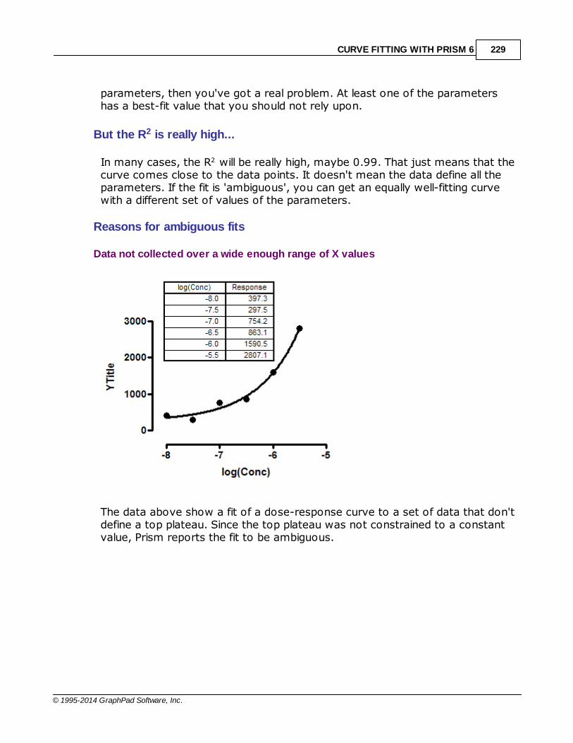
CURVE FITTING WITH PRISM 6 229
© 1995-2014 GraphPad Software, Inc.
parameters, then you've got a real problem. At least one of the parametershas a best-fit value that you should not rely upon.
But the R2 is really high...
In many cases, the R2 will be really high, maybe 0.99. That just means that thecurve comes close to the data points. It doesn't mean the data define all theparameters. If the fit is 'ambiguous', you can get an equally well-fitting curvewith a different set of values of the parameters.
Reasons for ambiguous fits
Data not collected over a wide enough range of X values
The data above show a fit of a dose-response curve to a set of data that don'tdefine a top plateau. Since the top plateau was not constrained to a constantvalue, Prism reports the fit to be ambiguous.

GraphPad Curve Fitting Guide230
© 1995-2014 GraphPad Software, Inc.
Model too complicated for the data
The data above fit fine to a standard dose-response curve. But if you try to fit itto a biphasic dose-response curve, Prism reports that the results areambiguous. The data follow a standard dose-response model just fine, with noevidence of a second component. So fitting to a biphasic model -- with twoEC50 values -- is ambiguous.
Model has redundant parameters
The simplest example would be fitting this model: Y= A + B + C*X. This modeldescribes a straight line with a slope equal to C and a Y intercept equal to thesum of A and B. But there is nothing in the data to fit A and B individually. Thereare an infinite number of pairs of values of A and B that lead to the same sum,so the same Y intercept. If Prism attempts to fit this model, it will conclude thatthe fit is ambiguous.
Prism cannot tell the difference between this case and the previous one. But thetwo cases are distinct. The model in this example has redundant parameters. Itdoesn't matter what the data look like, or how many data points you collect,fitting this model will always result in 'ambiguous' results, because two of theparameters are intertwined. In the previous example, the fit was ambiguouswith the example data set, but would not have been ambiguous with other datasets.
Checklist
Can you constrain any parameters to a constant value?

CURVE FITTING WITH PRISM 6 231
© 1995-2014 GraphPad Software, Inc.
Can you share one or more parameters among datasets?
Can you collect more data points, perhaps over a wider range of X values?
If your model has two phases or components, consider switching to a onephase or component model.
2.6.4.5 "Hit constraint"
What does "hit constraint" mean?
Prism reports "Hit constraint" when the best-fit value of one or moreparameters is right at the limit of a constraint.
When a fit hits a constraint, the results are unlikely to provide usefulinformation. If you had a solid reason to constrain a parameter within a rangeof values, it ought to end up in that range. If the fit hit the constraint limit, thatmeans the true best-fit value is some value forbidden by the constraint.
Prism does not compute confidence and prediction bands when a parameter hita constraint. The best-fit values are not a local minimum, so any attempt tocompute confidence or prediction bands would give misleading results. Prismdoes compute the confidence intervals for the other parameters (the ones thatdidn't hit a constraint) but these need to be viewed with caution.
When a fit ends up hitting a constraint, it is likely that you set the constraintincorrectly. So the first thing to do is make sure the constraint is sensible andcorrectly entered. For example, if you mistakenly set a constraint that a rateconstant K must be less than or equal to zero, Prism's nonlinear regressionmight converge with the best-fit value equalling zero and report that you hit theconstraint. Fix the constrain to be greater than or equal to zero, and the fit willwork fine.
Another possibility is to change the constraint from an inequality (Bottom>0) toa constant constraint (Bottom=0). You'll get the same parameter values, butdifference confidence intervals, and you can get confidence and predictionbands.
Checklist
Did you enter the constraint correctly? Did you mix up "<" and ">".

GraphPad Curve Fitting Guide232
© 1995-2014 GraphPad Software, Inc.
Did you enter the model correctly?
Are you asking Prism to do the impossible -- too many parameters for yourdata?
If your model has two phases or components, consider switching to a onephase or component model.
2.6.4.6 "Don't fit"
The top of the Diagnostics tab offers the choice to plot the curve defined by theinitial values of the parameters.
When you make this choice, the top of the results will show "Don't fit".
This is a very useful option to use when diagnosing problem fits. But you won'tlearn anything by looking at the results page. Instead, look at the graph. If thecurve goes near the points, then the initial values are OK. If the curve is farfrom the points, or follows a different shape altogether, then you know thatthere is a problem with the choice of model or initial values.
If you checked this option by mistake, go back to the Diagnostics tab andcheck the alternative choice ("Fit the curve.").
2.6.4.7 "Too few points"
Regression requires at least as many data points as parameters. So if you fit adose-response model with four parameters (Bottom, Top, logEC50, andHillSlope), you must have four or more points or Prism will simply report "toofew points".
Having as many points as parameters is the bare minimum. Prism will try to fitthe model, and will report a perfect fit , and so not be able to report standarderrors or confidence intervals. If there are only a few more points thatparameters, Prism is likely to end up with an ambiguous or not convergedfit.
233
228 227
CURVE FITTING WITH PRISM 6 233
© 1995-2014 GraphPad Software, Inc.
2.6.4.8 "Perfect fit"
Prism reports "perfect fit' when the curve goes through every point. The sum-of-squares is 0.0, and R2 is 1.00.
If you are testing nonlinear regression with made up values, add some randomscatter to make a better example.
If you are fitting actual data, and the fit is perfect, you either got very lucky orhave very few data points. It is not possible to compute the standard errorsand confidence intervals of the parameters when the fit is perfect, nor is itpossible to compare models.
2.6.4.9 "Impossible weights"
Prism reports "Impossible weighting" when weighting would lead to division byzero for one or more point. This can happen when you choose to weight by thereciprocal of Y, and the Y value of the curve equals zero at some X values.Since division by zero is impossible, Prism reports "Impossible weighting". Go tothe weights tab and choose a different weighting method .
Prism also reports "impossible weights" when the Y value of the curve isnegative for some values of X. If you weight by 1/Y, this would mean theweights would be negative. If you weight by 1/Y2, the weights would all bepositive, but points with Y near zero would get lots of weight, and points with Yvalues far from zero (in either direction) would get low weights, and thisdoesn't really make sense.
2.6.4.10 "Equation not defined"
When you enter a user-defined equation, you can write adifferent model for different data sets . If no model is definedfor certain data sets, the message "Equation not defined" willappear in the results for that data set, with no other results.
"Bad initial values"
"Interrupted"
"Not converged"
"Ambiguous"
"Hit constraint"
160
423
226
226
227
228
231

GraphPad Curve Fitting Guide234
© 1995-2014 GraphPad Software, Inc.
"Don't fit"
"Too few points"
"Perfect fit"
"Impossible weights"
"Equation not defined"
2.6.4.11 "Can't calculate"
If you ask Prism to use either the F test or the AICc method to compare twomodels, it will report "Can't calculate" if the two models have the same numberof parameters. This means it can't calculate the comparison between fits, notthat it can't fit the two models to the data.
Both these methods to compare models only make sense when the modelsbeing compared have different numbers of parameters, and so have differentnumbers of degrees of freedom. These methods are alternative methods ofdealing with the tradeoff between how well the model fits and how complicatedit is (assessed by the number of parameters).
If you want to compare two models with the same number of parameters,there is no need to use either the F test or AIC. Simply choose the model thatfits the data the best with the smallest sum-of-squares.
2.7 Models (equations) built-in to Prism
To use nonlinear regression, you need to choose a model. Inmany cases, especially if you are fitting pharmacological orphysiological data, you can choose one of Prism's built-inmodels described here.
Dose-response - Key concepts
Dose-response - Stimulation
Dose-response - Inhibition
Dose-response -- Special
Receptor binding - Key concepts
232
232
233
233
233
235
255
261
267
285

CURVE FITTING WITH PRISM 6 235
© 1995-2014 GraphPad Software, Inc.
Receptor binding - Saturation binding
Receptor binding - Competitive binding
Receptor binding - Kinetics
Enzyme kinetics -- Key concepts
Enzyme kinetics - Subtrate vs. velocity
Enzyme kinetics -- Inhibition
Exponential
Lines
Polynomial
Gaussian
Sine waves
Classic equations from prior versions of Prism
2.7.1 Dose-response - Key concepts
2.7.1.1 What are dose-response curves?
What are dose-response curves?
Dose-response curves can be used to plot the results of many kinds ofexperiments. The X axis plots concentration of a drug or hormone. The Y axisplots response, which could be almost any measure of biological function.
The term “dose” is often used loosely. In its strictest sense, the term onlyapplies to experiments performed with animals or people, where you administervarious doses of drug. You don't know the actual concentration of drug at itssite of action—you only know the total dose that you administered. However,the term “dose-response curve” is also used more loosely to describe in vitroexperiments where you apply known concentrations of drugs. The term“concentration-response curve” is a more precise label for the results of these
291
311
324
335
337
344
355
370
381
385
393
396

GraphPad Curve Fitting Guide236
© 1995-2014 GraphPad Software, Inc.
types of experiments. The term “dose-response curve” is occasionally usedeven more loosely to refer to experiments where you vary levels of someother variable, such as temperature or voltage.
X values are logarithm of doses or concentrations
Dose-response experiments typically use around 5-10 doses of agonist, equallyspaced on a logarithmic scale. For example, doses might be 1, 3, 10, 30, 100,300, 1000, 3000, and 10000 nM. When converted to logarithms (and roundeda bit), these values are equally spaced: 0.0, 0.5, 1.0, 1.5, 2.0, 2.5, 3.0, 3.5,and 4.0.
If you entered concentrations, instead of the logarithm of concentrations, youcan perform the transformation with Prism .
Y values are responses
In a dose-response curve, the Y values are responses. For example, theresponse might be enzyme activity, accumulation of an intracellular secondmessenger, membrane potential, secretion of a hormone, change in heart rate,or contraction of a muscle.
You can transform the Y values to new units by multiplying or dividing by aconstant. Use Prism's Transform analysis for this. Transforming to new units willnot fundamentally change the results of a curve fit.
In some cases, the transform from experimentally observed units to practicalunits is nonlinear. For example, a nonlinear transform is needed to convert theratio of two fluorescence values to concentrations of Ca++. Which Y valuesshould be used when fitting a dose-response curve? Nonlinear regressionassumes that all scatter around the curve is Gaussian, so you want to usewhatever units make that assumption most true. In many cases, this may behard to know.
2.7.1.2 The EC50
What is the EC50?
The EC50 is defined quite simply as the concentration of agonist that provokesa response halfway between the baseline (Bottom) and maximum response(Top). It is impossible to define the EC50 until you first define the baseline andmaximum response.
Depending on how you have normalized your data, the EC50 may not be thesame as the concentration that provokes a response of Y=50. For instance, in
244

CURVE FITTING WITH PRISM 6 237
© 1995-2014 GraphPad Software, Inc.
the example below, the data are normalized to percentage of maximumresponse, without subtracting a baseline. The baseline is about 20%, and themaximum is 100%, so the EC50 is the concentration of agonist that evokes aresponse of about 60% (halfway between 20% and 100%). The concentrationthat provokes a response of 50 in this experiment is not the EC50.
10 -9 10 -8 10 -7 10 -6 10 -5 10 -4 10 -3
0
25
50
75
100
EC50
[Agonist, M]
Resp
on
se
Perc
en
t o
f C
on
tro
l
Don't over interpret the EC50. It is simply the concentration of agonist requiredto provoke a response halfway between the baseline and maximum responses.Because the EC50 defines the location of the dose-response curve for aparticular drug, it is the most commonly used measure of an agonist’s potency.However, the EC50 is usually not the same as the Kd for the binding of agonistto its receptor -- it is not a direct measure of drug affinity.
The pEC50
The pEC50 is defined as the negative logarithm of the EC50. If the EC50 equals1 micromolar (10-6 molar), the log EC50 is –6 and the pEC50 is 6. There is noparticular advantage to expressing potency this way, but it is customary insome fields.
The IC50
In many experiments, you vary the concentration of an inhibitor. With moreinhibitor, the response decreases, so the dose-response curve goes downhill.With such experiments, the midpoint is often called the IC50 ("I" for inhibition)rather than the EC50 ("E" for effective). This is purely a difference in whichabbreviation is used, with no fundamental difference.
ECanything
A simple rearrangement of the equation lets you fit EC80 (or EC90 or

GraphPad Curve Fitting Guide238
© 1995-2014 GraphPad Software, Inc.
ECanything) instead of the EC50. Prism includes an equation that fits any ECvalue directly.
2.7.1.3 Confidence intervals of the EC50
The 95% confidence interval of the EC50 is not symmetrical
-9 -8 -7 -6 -5 -4 -3
0
1000
2000
Best-fit values
BOTTOM
TOP
LOGEC50
EC50
Std. Error
BOTTOM
TOP
LOGEC50
95% Confidence Intervals
BOTTOM
TOP
LOGEC50
EC50
351.9
1481
-6.059
8.7250e-007
101.4
99.29
0.2717
128.7 to 575.1
1263 to 1700
-6.657 to -5.461
2.2020e-007 to 3.4570e-006
log[Dose]
Re
sp
on
se
The sample data above were fit to a dose-response curve with a Hill slope of 1.The best-fit value for logEC50 is -6.059. Converting to the EC50 is no problem– simply take the antilog, which is 0.87 mM.
The standard error of the logEC50 is 0.2717. It is used to calculate a 95%confidence interval, which ranges from -6.657 to -5.461. Take the antilog of
283

CURVE FITTING WITH PRISM 6 239
© 1995-2014 GraphPad Software, Inc.
both of those limits to express that confidence interval on a concentration scale-- from 0.22 to 3.46 mM. This is the interval that Prism presents. Note that itis not centered on the best-fit value (0.87 mM). Switching from linear to logscale converted the symmetrical confidence interval into an asymmetricalinterval.
Keep in mind the fundamentals of a logarithmic axis. A distance along a log axisdoes not represent a consistent distance along a linear (standard) axis. Forexample, increasing the logEC50 1 unit from -9 to -8 increases the EC50 9nM(assuming the X values were entered as log Molar), while increasing thelogEC50 1 unit from -3 to -2 increases the EC50 by 9 mM, which equals9,000,000 nM.
If you fit the same data to an equation describing a dose-response curve interms of the EC50 rather than the logEC50, the EC50 remains 0.87 mM. Butnow Prism computes the SE of the EC50 (0.5459 mM), and uses this tocompute the 95% confidence interval of the EC50, which ranges from -0.3290to +2.074 mM. Note that the lower limit of the confidence interval is negative!Since the EC50 is a concentration, negative values are nonsense. Even settingaside the negative portion of the confidence interval, it includes all values fromzero on up, which isn't terribly useful.
The problem is that the uncertainty of the EC50 really isn't symmetrical,especially when you space your doses equally on a log scale. It only makessense to compute the 95% CI of the logEC50, and then transform bothconfidence limits to a concentration scale, knowing that the confidence intervalwill not be symmetrical on the concentration scale.
Do not transform the standard error of the logEC50
When some people see the SE of the logEC50, they are tempted to convertthis to the standard error of the EC50 by taking the antilog. This is invalid.
In the example, the SE of the logEC50 is 0.2717. The antilog of 0.2717 equals1.869. This value is not the SE of the EC50 and is really not a value that ishelpful to compute.
Averaging the EC50 from several experiments
The uncertainty is symmetrical when you express the midpoint of a dose-response curve as a logEC50, but is far from symmetrical (often) when youexpress it as the EC50. When pooling several experiments, therefore, it is bestto average the logEC50 values, which will give a different result than averagingthe EC50 values.

GraphPad Curve Fitting Guide240
© 1995-2014 GraphPad Software, Inc.
2.7.1.4 Hill slope
The usual steepness of a dose-response curve
Many dose-response curves follow the shape of a receptor binding curve. Asshown below, 81 times more agonist is needed to achieve 90% response thana 10% response.
0%
10%
90%
100%
81 fold
Log[Agonist]
Pe
rce
nt
Re
sp
on
se
Since the linkage between agonist binding and response can be very complex,any shape is possible. It seems surprising, therefore, that so many dose-response curves have shapes almost identical to receptor binding curves, evenwhen we know there are multiple steps between binding and measuredresponse. It turns out that no matter how many steps intervene betweenagonist binding and response, the dose-response curve will have the usualsteepness so long as each messenger binds to a single binding site according tothe law of mass action.
The slope factor or Hill slope
Some dose-response curves are steeper or shallower than the standard curve.The steepness is quantified by the Hill slope, also called a slope factor. A dose-response curve with a standard slope has a Hill slope of 1.0. A steeper curvehas a higher slope factor, and a shallower curve has a lower slope factor.
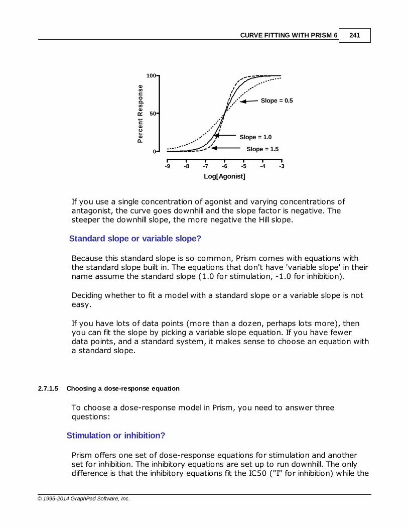
CURVE FITTING WITH PRISM 6 241
© 1995-2014 GraphPad Software, Inc.
-9 -8 -7 -6 -5 -4 -3
0
50
100
Slope = 1.5
Slope = 1.0
Slope = 0.5
Log[Agonist]
Pe
rce
nt
Re
sp
on
se
If you use a single concentration of agonist and varying concentrations ofantagonist, the curve goes downhill and the slope factor is negative. Thesteeper the downhill slope, the more negative the Hill slope.
Standard slope or variable slope?
Because this standard slope is so common, Prism comes with equations withthe standard slope built in. The equations that don't have 'variable slope' in theirname assume the standard slope (1.0 for stimulation, -1.0 for inhibition).
Deciding whether to fit a model with a standard slope or a variable slope is noteasy.
If you have lots of data points (more than a dozen, perhaps lots more), thenyou can fit the slope by picking a variable slope equation. If you have fewerdata points, and a standard system, it makes sense to choose an equation witha standard slope.
2.7.1.5 Choosing a dose-response equation
To choose a dose-response model in Prism, you need to answer threequestions:
Stimulation or inhibition?
Prism offers one set of dose-response equations for stimulation and anotherset for inhibition. The inhibitory equations are set up to run downhill. The onlydifference is that the inhibitory equations fit the IC50 ("I" for inhibition) while the

GraphPad Curve Fitting Guide242
© 1995-2014 GraphPad Software, Inc.
stimulation equations fit the EC50 ("E" for effective).
If the curve goes up hill, choose from the set of stimulation equations. If thecurve goes down hill, choose from the set of inhibition equations.
Standard slope or variable slope?
A huge variety of dose-response curves follow the same steepness as receptorbinding, so have a Hill slope of 1.00 (for stimulation) or -1.00 (for inhibition).Because this standard slope is so common, Prism comes with equations withthe standard slope built in. The equations that don't have 'variable slope' in theirname assume the standard slope.
If you have lots of data points (more than a dozen, perhaps lots more), thenyou can fit the slope by picking a variable slope equation. If you have fewerdata points, and a standard system, it makes sense to choose an equation witha standard slope.
Normalized or not?
If your data have been normalized so the curve runs from Y= 0 to Y=100, youmay wish to choose a normalized model. These models don't fit the bottomand top plateaus, but rather force the bottom plateau to equal 0 and the topplateau to equal 100. Only choose a 'normalized response' equation when youhave determined the values that define 0 and 100 very precisely. Just becausethe data have been normalizeddoesn't mean to have to constrain the curve inthat way.
Special dose-response models
Prism has a set of special models used for special dose-response situations:
Asymmetrical (five parameter)
Biphasic dose-response
Bell-shaped dose-response
Operational model - Depletion
Operational model - Partial agonist
Gaddum/Schild EC50 shift
240
243
267
269
271
272
275
277

CURVE FITTING WITH PRISM 6 243
© 1995-2014 GraphPad Software, Inc.
Allosteric EC50 shift
ECanything
2.7.1.6 Pros and cons of normalizing the data
The dose-response model has four parameters: the bottom plateau, the topplateau, the EC50, and the slope factor (which is often constrained to astandard value).
The main goal of fitting the dose-response curve in many situations is todetermine the best-fit value of the EC50, which is the concentration thatprovokes a response halfway between the top and bottom plateaus. If thoseplateaus are not well defined, the EC50 will be very uncertain. Think of it thisway: If you have not defined "100" and "0" very precisely, you also have notdefined "50" precisely, and therefore cannot determine the EC50 precisely.
One way to solve the problem is to constrain the Top or Bottom, or both, tocontrol values. Another alternative is to normalize your data so responses runfrom 0 to 100, and then choose a "normalized response" model. These modelsdon't fit the bottom and top plateaus, but rather force the bottom plateau toequal 0 and the top plateau to equal 100. Only choose a 'normalized response'equation when you have determined the values that define 0 and 100 veryprecisely.
Prism makes it easy to normalize the data so the values run from 0% to 100%. Simply click Analyze, choose the Normalize analysis., and define how 0% and100% are defined. When fitting a dose-response curve, you can fit either theraw data or normalized data.
Notes:
It is not necessary to normalize before fitting dose-response data. In many
cases, it is better to show the actual data.
You can only plot several different dose-response curves on one graph using
one axis when they are comparable. If the different experiments measureddifferent variables, normalizing puts them into comparable units. This can beuseful.
Whether or not you choose to normalize your data, you still need to choose
how to fit the data. Do you want Prism to find best-fit values for the Top andBottom plateaus? Or do you want those plateaus to be determined by controldata?
281
283

GraphPad Curve Fitting Guide244
© 1995-2014 GraphPad Software, Inc.
If you normalize your data, you can choose one of the normalized dose-
response equations. These constrain the the curve to run from 0% to 100%.This kind of constraint only makes sense, when 0% and 100% are defined bygood control data. If the definitions of 0% and 100% are ambiguous, then sois the definition of "50%", and thus the EC50 is also ambiguous.
Just because you chose to normalize your data doesn't mean you must
constrain the curve to run from 0 to 100%. You may prefer to have Prism fitthose two plateaus.
If you don't normalize your data, you can use the Constrain tab to fix Top
and Bottom to values determined from control experiments. So the decisionto constrain Top and Bottom is quite distinct from the decision to normalizeyour data before fitting.
It is possible, and can be reasonable, to fix one of those parameters (Top or
Bottom) to a constant value but not the other.
If you normalize, don't also choose to differentially weight the data .
2.7.1.7 Converting concentration to log(concentration)
Transforming X values with Prism
All the dose-response equations built-in to Prism expect the X values to be thelogarithm of dose or concentration.
If you entered actual doses or concentrations, instead of their logarithms, usePrism to transform the X values.
1.From the data table, click Analyze and then choose Transform, which is thevery first analysis listed on the Analyze dialog.
2.On the Transform dialog, check the option to transform X, and chooseX=log(X) .At the bottom of the dialog, check the option: Create a newgraph of the results.
35

CURVE FITTING WITH PRISM 6 245
© 1995-2014 GraphPad Software, Inc.
3. Go to the newly created graph.
4.Click Analyze, choose nonlinear regression, and then choose the dose-response curve.
2.7.1.8 The term "logistic"
The terms logistic has three meanings which have little relationship to eachother (1).
Meaning 1: Logistic population growth
The term "logistic" was first invented in the nineteenth century to describepopulation growth curves. The idea is pretty simple. Population growth islimited, so can't ever exceed some value we'll call Nmax. The rate of change ofpopulation at any time t is proportional to the number of individuals alive at that

GraphPad Curve Fitting Guide246
© 1995-2014 GraphPad Software, Inc.
time (Nt). But population growth slows down as it reaches the maximum, so isalso proportional to (Nmax - Nt). So the rate of change of population isproportional to Nt(Nmax - Nt).
Integrate that differential equation, and the result is called a logistic equation. Itdefines a sigmoidal shaped curve that defines the population at any time. Themodel has three parameters: the starting population, the maximum population,and the time it takes to reach half-maximal. Sometimes it is modified to add afourth parameter to define the steepness of the curve.
This curve was used by demographers in the past, but actually doesn't do avery good job of describing the growth of human populations. It is still used tomodel the growth of tumors, and to model the fraction of a population thatuses a new product (like a mobile phone).
This model is also used for autocatalytic reactions, where the product of thereaction is also a catalyst for that reaction. With this kind of reaction, the rateof product accumulation is proportional to the concentration of product alreadyproduced times the concentration of remaining substrate. This has the samemathematical form as the population growth model. The graph is identical tothe one above, except the Y-axis would be the concentration of the productproduced by the enzyme reaction (instead of population).
Meaning 2: "Logistic" dose-response curves
Bindslev reviews the history of the many equations used to describe doseresponse curves(2). A common equation, based on work by Hill, defines aresponse as a function of the minimum response, the maximum response, theconcentration required to evoke a response half-way between the minimumand maximum (the EC50), and a parameter that describes how steep thecurve is. In Prism, this equation is called the log(agonist) vs response curve --Variable slope (four parameters).

CURVE FITTING WITH PRISM 6 247
© 1995-2014 GraphPad Software, Inc.
Response at any dose is defined by an equation with four parameters:minimum response, maximum response, the log(EC50), and the slope factor(also called the Hill slope). Surprisingly, this equation has the samemathematical form as the logistic equation describing population growth, eventhough the two uses are entirely different. For this reason, the dose-responseequation is sometimes called a "logistic" equation. Since there are fourparameters, it is sometimes called the four parameter logistic equation,abbreviated 4PL.
This dose-response model describes many systems, but it is purely empirical. Itdoes not correspond to any molecular model (except, perhaps, when the Hillslope is an integer).
Note the huge differences between the use of a logistic equation to describepopulation growth, and its use to describe dose-response curves.
The X axis of the population growth curve curve is time. The X axis of the
dose-response curve is the logarithm of dose or concentration.
The equation for population growth comes from theory. The equation for
dose-response relationships is empirical.
Despite its name, no logarithms are used in the logistic equation for
population growth. The X axis of the logistic dose-response curve is thelogarithm of dose or concentration.
Meaning 3: Logistic regression
The third use of the word logistic, completely unrelated to the other two uses,is logistic regression. This is a multiple regression method used when theoutcome (dependent variable) has two possible outcomes. The point of theequation is to predict the probability, P, of an outcome from a set ofindependent variables. To create a model that always predicts a value for P that
GraphPad Curve Fitting Guide248
© 1995-2014 GraphPad Software, Inc.
is between 0 and 1 the logistic regression model actually predicts the naturallogarithm of the odds. The function that computes the natural logarithm of theodds from a fraction is called the logit function (pronounced with a long O and asoft G), so regression used to predict the logit of a probability from multipleindependent variables is called logistic regression.
References
1. J.S. Cramer. The origins and development of the logit model. Chapter 9 ofLogit models from economics and other fields, Cambridge University Press,2003
2. N. Bindslev, Hill in Hell (pdf), Chapter 10 of Drug-Acceptor Interactions,ISBN: 978-91-977071-0-7
2.7.1.9 50% of what? Relative vs absolute IC50.
IC50 can be ambiguous
50% of what? There can be more than one answer in some situations.
The concepts of IC50 is fundamental to pharmacology. The IC50 is theconcentration of an inhibitor where the response (or binding) is reduced by half.Seems simple enough. But when you actually go to fit data to determine thesevalues, there are several complexities and ambiguities.
The rest of this article is about IC50 (I for inhibition, for downward slopingdose-response curves). All the ideas can be applied to stimulatory curves andEC50 (E for effective) as well. Just stand on your head when you view thefigures!.
The ideal situation
This figure shows an ideal situation:

CURVE FITTING WITH PRISM 6 249
© 1995-2014 GraphPad Software, Inc.
The green symbols show measurements made with controls. The ones on theleft (Blank) have no inhibitor, so define "100%". The ones on the right are inthe presence of a maximal concentration of a standard inhibitor, so define"0%". The data of the experimental dose-response curve (red dots) extend allthe way between the two control values.
When fitting this curve, you need to decide how to fit the top plateau of thecurve. You have three choices:
Fit the data only, ignoring the Blank control values.
Average the Blank control values, and set the parameter Top to be a constant
value equal to the mean of the blanks.
Enter the blank values as if they were part of the dose-response curve.
Simply enter a low dose, perhaps 10-10 or 10-11. You can't enter zero,because zero is not defined on a log scale.
The results will be very similar with any of these methods, because the dataform a complete dose-response curve with a clear top plateau that isindistinguishable from the blank. I prefer the third method, as it analyzes all thedata, but that is not a strong preference.
Similarly, there are three ways to deal with the bottom plateau: Fit the dataonly, set Bottom to be a constant equal to the average of the NS controls,and put the NS controls into the fit as if they were a very high concentration ofinhibitor.

GraphPad Curve Fitting Guide250
© 1995-2014 GraphPad Software, Inc.
That is the ideal situation. There is no ambiguity about what IC50 means.
A potentially ambiguous situation
The graph below shows an unusual situation where the inhibition curve plateauswell above the control values (NS) defined by a high concentration of astandard drug. This leads to alternative definitions of IC50.
Clearly, a single value cannot summarize such a curve. You'd need at least twovalues, one to quantify the middle of the curve (the drug's potency) and one toquantify how low it gets (the drug's maximum effect).
The graph above shows two definitions of the IC50.
The relative IC50 is by far the most common definition, and the adjectiverelative is usually omitted. It is the concentration required to bring the curvedown to point half way between the top and bottom plateaus of the curve.The NS values are totally ignored with this definition of IC50. This definition isthe one upon which classical pharmacological analysis of agonist and antagonistinteractions is based. With appropriate consideration of the biological systemand concentrations of interacting ligands, estimated Kd values can often bederived from the IC50 value defined this way (not so for the "so-called absoluteIC50" mentioned below).
The concentration that provokes a response halfway between the Blank andthe NS value is sometimes called the absolute IC50, The horizontal dotted

CURVE FITTING WITH PRISM 6 251
© 1995-2014 GraphPad Software, Inc.
lines show how 100% and 0% are defined, which then defines 50%. This termis not entirely standard. Since this value does not quantify the potency of adrug, the authors of the International Union of Pharmacology Committee onReceptor Nomenclature (1) think that the concept of absolute IC50 (and thatterm) is not useful (R. Neubig, personal communication). I agree.
The concept (but not the term "absolute IC50") is used to quantify drugs thatslow cell growth. The abbreviation GI50 is used for what we call here theabsolute IC50. It is also used by the Environmental Protection Agency (EPA) in evaluating endocrine disrupters (Appendix A). That document uses the termIC50 to refer to the absolute IC50, and the term EC50 to refer to the relativeIC50. It doesn't use the terms relative and absolute.
If you really want to use the absolute IC50, the next page has instructions forfitting a curve to find it .
Reference
1. R. R. Neubig et al. International Union of Pharmacology Committee onReceptor Nomenclature and Drug Classification. XXXVIII. Update on terms andsymbols in quantitative pharmacology. Pharmacol Rev (2003) vol. 55 (4) pp.597-606
Download the Prism file used to create all the graphs in this article.
2.7.1.10 Fitting the absolute IC50
Fitting a dose-response curve to find the absolute IC50
The concept of an absolute IC50 is not standard, and many find it not to beuseful. But if you do, it is not hard to fit a curve to determine it. Appendix A of this EPA document, give the needed equation (which I have generalized a bit,so not require that the data already be normalized).
Fifty=(Top+Baseline)/2Y= Bottom + (Top-Bottom)/(1+10^((LogIC50-X)*HillSlope + log((Top-Bottom)/(Fifty-Bottom)-1)))
Note the distinction between the parameter Bottom and Baseline. Bottom is theY value of the bottom plateau of the curve itself. Baseline is the Y value thatdefines 0% -- maximal inhibition by a standard drug. You'll definitely want toconstrain Baseline to be a constant value based on controls. You may alsowant to constrain Top.
Download the Prism file that fits that equation to make the graph shown above.
251

GraphPad Curve Fitting Guide252
© 1995-2014 GraphPad Software, Inc.
When fitting data to that equation, don't forget to constrain Baseline and Top toappropriate values determined by controls. Additionally, this file containsanother graph where the data are already normalized to run from 0 to 100%.These data are fit to a simpler equation where Baseline is set to equal zero, andTop is set to equal 100. These are hard wired into the equation, so you don'thave to remember to constrain those two parameters to constant values.
An alternative approach for normalized data
Here is an alternative approach you can use if your data are normalized. It doesnot require entering a user-defined equation.
1.Make sure that your data are normalized to some controls. That means theresponse at the left end (low concentrations) is near 100%, and theresponse at higher concentrations is above 0%. If the response plateaus at0%, then an absolute and relative IC50 are the same, and you can just fitthe usual dose-response curve to find the IC50.
2.At the bottom of the data table, add a new row of data. Enter 50 into each Ycolumn. Leave X blank for this row.
3.Use nonlinear regression to fit the data to the log(inhibitor) vs. response(variable slope) curve.
4.On the first (fit) tab of the nonlinear regression dialog, check the option: "Interpolate unknowns from standard curve." Of course, these data are not astandard curve, and there are unknowns. But this option asks Prism tointerpolate the X value of the curve when Y=50.
5.On the Constrain tab, consider constraining Top to have a constant value of100. If you have used good controls to normalize your data, then you knowthe top plateau of the curve has to be Y=100, so should tell Prism to use thatconstraint.
6.The IC50 reported as part of the main results table will be the relative IC50.
7.Look on the additional results page of interpolated results to see the value ofX when Y=50. This is the absolute IC50.

CURVE FITTING WITH PRISM 6 253
© 1995-2014 GraphPad Software, Inc.
2.7.1.11 Incomplete dose-respone curves
Any attempt to determine an IC50 by fitting a curve to the data in the graphabove will be useless. Prism might, or might not, be able to fit a dose-responsecurve to the data. But if the curve fits, the value of the IC50 is likely to bemeaningless and have a very wide confidence interval. The data simply don'treally define a top plateau (which would define 100) and certainly doesn'tprovide even a hint of a bottom plateau (which would define 0). If data haven'tdefined 100 or 0, then 50 is undefined too, as is the IC50.
If you also have control values that define 100 and 0, then the curve can beeasily fit. The curve below was created by fitting a dose response curve, butconstraining the Top plateau to be a constant value equal to the mean of theBlanks values, and the Bottom plateau equal to the mean of the NS values. Note that the blank and NS values are shown in green.

GraphPad Curve Fitting Guide254
© 1995-2014 GraphPad Software, Inc.
The value of the IC50 fit this way only makes sense if you assume that higherconcentrations of the inhibitor would eventually inhibit down to the NS values.That is an assumption that can't be tested with the data at hand.
The distinction between relative and absolute IC50 doesn't really apply tothese data. Because the data don't define a bottom plateau, the IC50 can onlybe defined relative to the NS control values.
2.7.1.12 Troubleshooting fits of dose-response curves
First consult the analysis checklists
If your goal is to interpolate from the standard curve, look at the analysis checklist designedfor that purpose .
If your goal is to fit a model to determine parameter values, review the general analysischecklist for fitting a model .
Questions to ask about dose-response curves
Are the X values logarithms of concentrations? If not, use the Transform analysis to make anew results table where the X values are logarithms. Note that stretching an axis to a logscale is not at all the same thing. Prism's nonlinear regression fits the values it is given.Using the Format Axis dialog to stretch the X axis to a logarithmic scale does not changethe values the curve fitter sees.
Is the top plateau defined by the data? If not, can it be constrained? If the top plateau is notdefined either by the data or by a constraint, then any fit of a dose-response curve is unlikelyto be useful.
248
223
218

CURVE FITTING WITH PRISM 6 255
© 1995-2014 GraphPad Software, Inc.
Is the bottom plateau defined by the data? If not, can it be constrained? If the bottomplateau is not defined either by the data or by a constraint, then any fit of a dose-responsecurve is unlikely to be useful.
Were the data normalized? To what values? If the data were normalized, considerconstraining the top and bottom plateaus to be 0 and 1 (or 100) in the Constraint tab?
Hill slope fixed? A Hill slope of 1.0 or -1.0 is commonly seen in many systems, but not all.
Four parameter assumes symmetry. The usual equations to fit dose response curves havefour parameters (top, bottom, EC50, Hill Slope), and define symmetrical curves. You canchoose an equation that adds a fifth parameter to fit asymmetrical curves .
2.7.2 Dose-response - Stimulation
2.7.2.1 Equation: log(agonist) vs. response
Introduction
Many log(dose) vs. response curves follow the familiar symmetrical sigmoidalshape. The goal is to determine the EC50 of the agonist - the concentrationthat provokes a response half way between the basal (Bottom) response andthe maximal (Top) response.
This model assumes that the dose response curve has a standard slope, equalto a Hill slope (or slope factor) of 1.0. This is the slope expected when a ligandbinds to a receptor following the law of mass action, and is the slope expectedof a dose-response curve when the second messenger created by receptorstimulation binds to its receptor by the law of mass action. If you don't havemany data points, consider using the standard slope model. If you have lots ofdata points, pick the variable slope model to determine the Hill slope from thedata.
This equation is sometimes called a three parameter dose-response curve. Ifyou also fit the Hill slope, then it is a four parameter equation.
Step by step
Create an XY data table. Enter the logarithm of the concentration of the agonistinto X. Enter response into Y in any convenient units. Enter one data set intocolumn A, and use columns B, C... for different treatments, if needed.
If you prefer to enter concentrations, rather than the logarithm of
267

GraphPad Curve Fitting Guide256
© 1995-2014 GraphPad Software, Inc.
concentrations, use Prism to transform the X values to logs .
From the data table, click Analyze, choose nonlinear regression, choose thepanel of equations "Dose-response curves - Stimulation" and then choose theequation log(Agonist) vs. response.
If you have subtracted off any basal response, consider constraining Bottom toa constant value of 0.
Model
Y=Bottom + (Top-Bottom)/(1+10^((LogEC50-X)))
Interpret the parameters
EC50 is the concentration of agonist that gives a response half way betweenBottom and Top. This is not the same as the response at Y=50. Depending onwhich units Y is expressed in, and the values of Bottom and Top, the EC50 maygive a response nowhere near "50". Prism reports both the EC50 and its log.
Top and Bottom are plateaus in the units of the Y axis.
2.7.2.2 Equation: log(agonist) vs. response -- Variable slope
Introduction
Many log(dose) response curves follow the familiar symmetrical sigmoidalshape. The goal is to determine the EC50 of the agonist - the concentrationthat provokes a response half way between the basal (Bottom) response andthe maximal (Top) response.
Many dose-response curves have a standard slope of 1.0. This model does not
244

CURVE FITTING WITH PRISM 6 257
© 1995-2014 GraphPad Software, Inc.
assume a standard slope but rather fits the Hill Slope from the data, and so iscalled a Variable slope model. This is preferable when you have plenty of datapoints. It is also called a four-parameter dose-response curve, or four-parameter logistic curve, abbreviated 4PL.
Step by step
Create an XY data table. Enter the logarithm of the concentration of the agonistinto X. Enter response into Y in any convenient units. Enter one data set intocolumn A, and use columns B, C... for different treatments, if needed.
If you prefer to enter concentrations, rather than the logarithm ofconcentrations, use Prism to transform the X values to logs .
From the data table, click Analyze, choose nonlinear regression, choose thepanel of equations "Dose-response curves - Stimulation" and then choose theequation "log(Agonist) vs. response -- Variable slope".
Consider constraining the parameter HillSlope to its standard values of 1.0. Thisis especially useful if you don't have many data points, and therefore cannot fitthe slope very well.
If you have subtracted off any basal response, consider constraining Bottom toa constant value of 0.
Model
Y=Bottom + (Top-Bottom)/(1+10^((LogEC50-X)*HillSlope))
Interpret the parameters
EC50 is the concentration of agonist that gives a response half way betweenBottom and Top. This is not the same as the response at Y=50. Depending onwhich units Y is expressed in, and the values of Bottom and Top, the EC50 maygive a response nowhere near "50". Prism reports both the EC50 and its log.
244

GraphPad Curve Fitting Guide258
© 1995-2014 GraphPad Software, Inc.
HillSlope describes the steepness of the family of curves. A HillSlope of 1.0 isstandard, and you should consider constraining the Hill Slope to a constantvalue of 1.0. A Hill slope greater than 1.0 is steeper, and a Hill slope less than1.0 is shallower.
Top and Bottom are plateaus in the units of the Y axis.
2.7.2.3 Equation: log(agonist) vs. normalized response
Introduction
Many log(dose) vs. response curves follow the familiar symmetrical sigmoidalshape.
If you have good control data, it can make sense to normalize the responseto run between 0% and 100%. This model assumes that the data have beennormalized, so forces the curve to run from 0% to 100%. The goal is todetermine the EC50 of the agonist - the concentration that provokes aresponse equal to 50%.
It only makes sense to fit a normalized model when you are sure you havedefined 0% and 100% quite accurately. If your data define a completesigmoidal curve, it is best to fit the entire curve and let Prism fit the Top andBottom plateaus . If your data don't form a full sigmoidal curve, but you candefine the bottom and top by solid control data, then fitting to a normalizedmodel is preferable.
This model assumes that the dose response curve has a standard slope, equalto a Hill slope (or slope factor) of 1.0. This is the slope expected when a ligandbinds to a receptor following the law of mass action, and is the slope expectedof a dose-response curve when the second (and third...) messengers createdby receptor stimulation binds to its receptor by the law of mass action. If youdon't have many data points, consider using the standard slope model. If youhave lots of data points, pick the variable slope model to determine the Hillslope from the data.
Step by step
Create an XY data table. Enter the logarithm of the concentration of the agonistinto X. Enter response into Y in any convenient units. Enter one data set intocolumn A, and use columns B, C... for different treatments, if needed.
If you prefer to enter concentrations, rather than the logarithm of
256

CURVE FITTING WITH PRISM 6 259
© 1995-2014 GraphPad Software, Inc.
concentrations, use Prism to transform the X values to logs .
From the data table, click Analyze, choose nonlinear regression, choose thepanel of equations "Dose-response curves - Stimulation" and then choose theequation "log(Agonist) vs. normalized response".
Model
Y=100/(1+10^((LogEC50-X)))
Interpret the parameter
EC50 is the concentration of agonist that gives a response half way betweenBottom and Top. This is not the same as the response at Y=50. Depending onwhich units Y is expressed in, and the values of Bottom and Top, the EC50 maygive a response nowhere near "50". Prism reports both the EC50 and its log.
2.7.2.4 Equation: log(agonist) vs. normalized response -- Variable slope
Introduction
Many log(dose) response curves follow the familiar symmetrical sigmoidalshape.
If you have good control data, it can make sense to normalize the response torun between 0% and 100%. This model assumes that the data have been normalized, so forces the curve to run from 0% to 100%. The goal is todetermine the EC50 of the agonist - the concentration that provokes aresponse equal to 50%.
244
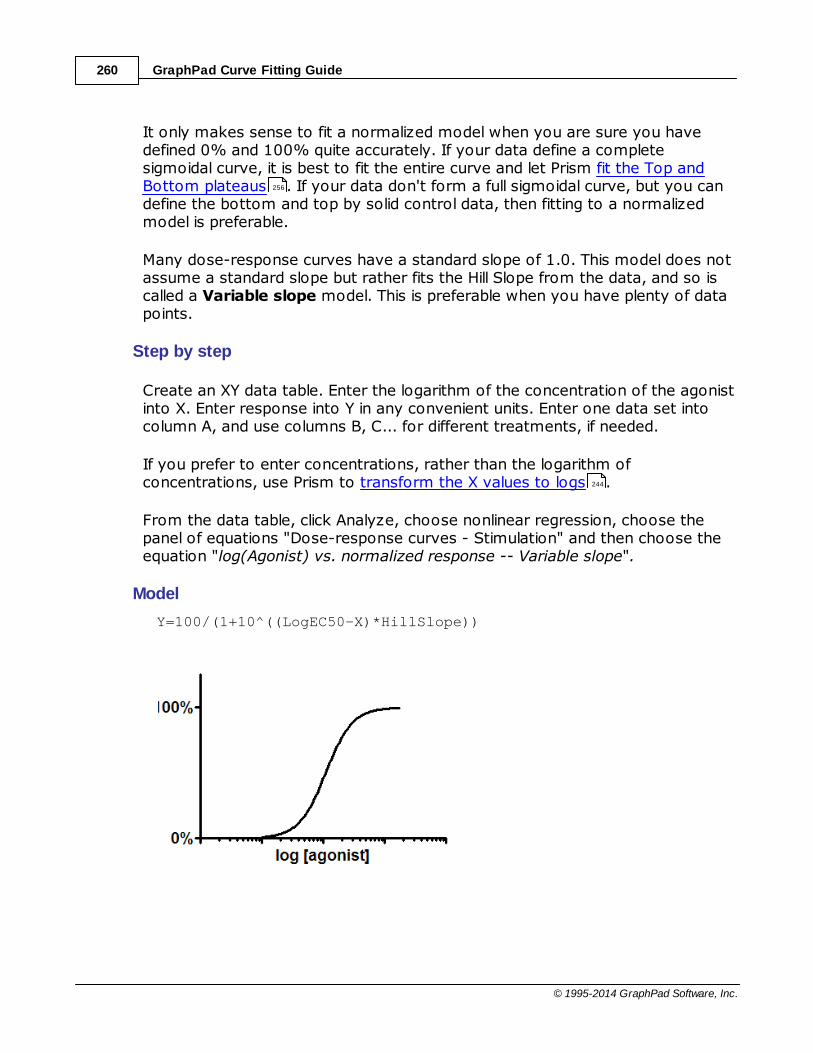
GraphPad Curve Fitting Guide260
© 1995-2014 GraphPad Software, Inc.
It only makes sense to fit a normalized model when you are sure you havedefined 0% and 100% quite accurately. If your data define a completesigmoidal curve, it is best to fit the entire curve and let Prism fit the Top andBottom plateaus . If your data don't form a full sigmoidal curve, but you candefine the bottom and top by solid control data, then fitting to a normalizedmodel is preferable.
Many dose-response curves have a standard slope of 1.0. This model does notassume a standard slope but rather fits the Hill Slope from the data, and so iscalled a Variable slope model. This is preferable when you have plenty of datapoints.
Step by step
Create an XY data table. Enter the logarithm of the concentration of the agonistinto X. Enter response into Y in any convenient units. Enter one data set intocolumn A, and use columns B, C... for different treatments, if needed.
If you prefer to enter concentrations, rather than the logarithm ofconcentrations, use Prism to transform the X values to logs .
From the data table, click Analyze, choose nonlinear regression, choose thepanel of equations "Dose-response curves - Stimulation" and then choose theequation "log(Agonist) vs. normalized response -- Variable slope".
Model
Y=100/(1+10^((LogEC50-X)*HillSlope))
256
244

CURVE FITTING WITH PRISM 6 261
© 1995-2014 GraphPad Software, Inc.
Interpret the parameters
EC50 is the concentration of agonist that gives a response half way betweenBottom and Top. This is not the same as the response at Y=50. Depending onwhich units Y is expressed in, and the values of Bottom and Top, the EC50 maygive a response nowhere near "50". Prism reports both the EC50 and its log.
HillSlope describes the steepness of the family of curves. A HillSlope of 1.0 isstandard, and you should consider constraining the Hill Slope to a constantvalue of 1.0.
2.7.3 Dose-response - Inhibition
2.7.3.1 Equation: log(inhibitor) vs. response
Introduction
Many log(inhibitor) vs. response curves follow the familiar symmetricalsigmoidal shape. The goal is to determine the IC50 of the inhibitor - theconcentration that provokes a response half way between the maximal (Top)response and the maximally inhibited (Bottom) response.
This model assumes that the dose response curves has a standard slope,equal to a Hill slope (or slope factor) of -1.0. This is the slope expected when aligand binds to a receptor following the law of mass action, and is the slopeexpected of a dose-response curve when the second messenger created byreceptor stimulation binds to its receptor by the law of mass action. If youdon't have many data points, consider using the standard slope model. If youhave lots of data points, pick the variable slope model to determine the Hillslope from the data.
Step by step
Create an XY data table. Enter the logarithm of the concentration of theinhibitor into X. Enter response into Y in any convenient units. Enter one dataset into column A, and use columns B, C... for different treatments, if needed.
If you prefer to enter concentrations, rather than the logarithm ofconcentrations, use Prism to transform the X values to logs . 244

GraphPad Curve Fitting Guide262
© 1995-2014 GraphPad Software, Inc.
From the data table, click Analyze, choose nonlinear regression, choose thepanel of equations "Dose-response curves - Inhibition" and then choose theequation "log(inhibitor) vs. response".
If you have subtracted off any basal response, consider constraining Bottom toa constant value of 0.
Model
Y=Bottom + (Top-Bottom)/(1+10^((X-LogIC50)))
Interpret the parameters
IC50 is the concentration of agonist that gives a response half way betweenBottom and Top. This is not the same as the response at Y=50. Depending onwhich units Y is expressed in, and the values of Bottom and Top, the IC50 maygive a response nowhere near "50". Prism reports both the IC50 and its log.
Top and Bottom are plateaus in the units of the Y axis.
2.7.3.2 Equation: log(inhibitor) vs. response -- Variable slope
Introduction
Many log(inhibitor) vs. response curves follow the familiar symmetricalsigmoidal shape. The goal is to determine the IC50 of the inhibitor - theconcentration that provokes a response half way between the maximal (Top)response and the maximally inhibited (Bottom) response.

CURVE FITTING WITH PRISM 6 263
© 1995-2014 GraphPad Software, Inc.
Many inhibitory dose-response curves have a standard slope of -1.0. Thismodel does not assume a standard slope but rather fits the Hill Slope from thedata, and so is called a Variable slope model. This is preferable when you haveplenty of data points. It is also called a four-parameter dose-response curve,or four-parameter logistic curve, abbreviated 4PL.
Step by step
Create an XY data table. Enter the logarithm of the concentration of theinhibitor into X. Enter response into Y in any convenient units. Enter one dataset into column A, and use columns B, C... for different treatments, if needed.
If you prefer to enter concentrations, rather than the logarithm ofconcentrations, use Prism to transform the X values to logs .
From the data table, click Analyze, choose nonlinear regression, choose thepanel of equations "Dose-response curves - Inhibition" and then choose theequation "log(inhibitor) vs. response -- Variable slope".
If you have subtracted off any basal response, consider constraining Bottom toa constant value of 0.
Model
Y=Bottom + (Top-Bottom)/(1+10^((LogIC50-X)*HillSlope))
Interpret the parameters
IC50 is the concentration of agonist that gives a response half way betweenBottom and Top. This is not the same as the response at Y=50. Depending onwhich units Y is expressed in, and the values of Bottom and Top, the IC50 maygive a response nowhere near "50". Prism reports both the IC50 and its log.
244
GraphPad Curve Fitting Guide264
© 1995-2014 GraphPad Software, Inc.
HillSlope describes the steepness of the family of curves. A HillSlope of -1.0 isstandard, and you should consider constraining the Hill Slope to a constantvalue of -1.0. A Hill slope more negative than -1 (say -2) is steeper.
Top and Bottom are plateaus in the units of the Y axis.
2.7.3.3 Equation: log(inhibitor) vs. normalized response
Introduction
Many log(inhibitor) vs. response curves follow the familiar symmetricalsigmoidal shape.
If you have good control data, it can make sense to normalize the responseto run between 0% and 100%. This model assumes that the data have beennormalized, so forces the curve to run from 100% down to 0%. The goal is todetermine the IC50 of the inhibitor - the concentration that provokes aresponse equal to 50%.
It only makes sense to fit a normalized model when you are sure you havedefined 0% and 100% quite accurately. If your data define a completesigmoidal curve, it is best to fit the entire curve and let Prism fit the Top andBottom plateaus . If your data don't form a full sigmoidal curve, but you candefine the bottom and top by solid control data, then fitting to a normalizedmodel is preferable.
This model assumes that the dose response curve has a standard slope, equalto a Hill slope (or slope factor) of -1.0. This is the slope expected when a ligandbinds to a receptor following the law of mass action, and is the slope expectedof a dose-response curve when the second messenger created by receptorstimulation binds to its receptor by the law of mass action. If you don't havemany data points, consider using the standard slope model. If you have lots ofdata points, pick the variable slope model to determine the Hill slope from thedata.
Step by step
Create an XY data table. Enter the logarithm of the concentration of theinhibitor into X. Enter response into Y in any convenient units. Enter one dataset into column A, and use columns B, C... for different treatments, if needed.
If you prefer to enter concentrations, rather than the logarithm ofconcentrations, use Prism to transform the X values to logs .
261
244

CURVE FITTING WITH PRISM 6 265
© 1995-2014 GraphPad Software, Inc.
From the data table, click Analyze, choose nonlinear regression, choose thepanel of equations "Dose-response curves - Inhibition" and then choose theequation "log(inhibitor) vs. normalized response".
Model
Y=100/(1+10^((X-LogIC50)))
Interpret the parameter
IC50 is the concentration of agonist that gives a response half way betweenBottom and Top. This is not the same as the response at Y=50. Depending onwhich units Y is expressed in, and the values of Bottom and Top, the IC50 maygive a response nowhere near "50". Prism reports both the IC50 and its log.
2.7.3.4 Equation: log(inhibitor) vs. normalized response -- Variable slope
Introduction
Many log(inhibitor) vs. response curves follow the familiar symmetricalsigmoidal shape.
If you have good control data, it can make sense to normalize the responseto run between 0% and 100%. This model assumes that the data have beennormalized, so forces the curve to run from 100% down to 0%. The goal is todetermine the IC50 of the inhibitor - the concentration that provokes aresponse equal to 50%.
It only makes sense to fit a normalized model when you are sure you havedefined 0% and 100% quite accurately. If your data define a complete

GraphPad Curve Fitting Guide266
© 1995-2014 GraphPad Software, Inc.
sigmoidal curve, it is best to fit the entire curve and let Prism fit the Top andBottom plateaus . If your data don't form a full sigmoidal curve, but you candefine the bottom and top by solid control data, then fitting to a normalizedmodel is preferable.
Many inhibitory dose-response curves have a standard slope of -1.0. Thismodel does not assume a standard slope but rather fits the Hill Slope from thedata, and so is called a Variable slope model. This is preferable when you haveplenty of data points.
Step by step
Create an XY data table. Enter the logarithm of the concentration of theinhibitor into X. Enter response into Y in any convenient units. Enter one dataset into column A, and use columns B, C... for different treatments, if needed.
If you prefer to enter concentrations, rather than the logarithm ofconcentrations, use Prism to transform the X values to logs .
From the data table, click Analyze, choose nonlinear regression, choose thepanel of equations "Dose-response curves - Inhibition" and then choose theequation "log(inhibitor) vs. normalized response -- variable slope".
Model
Y=100/(1+10^((LogIC50-X)*HillSlope)))
Interpret the parameters
IC50 is the concentration of agonist that gives a response half way betweenBottom and Top. This is not the same as the response at Y=50. Depending onwhich units Y is expressed in, and the values of Bottom and Top, the IC50 may
261
244
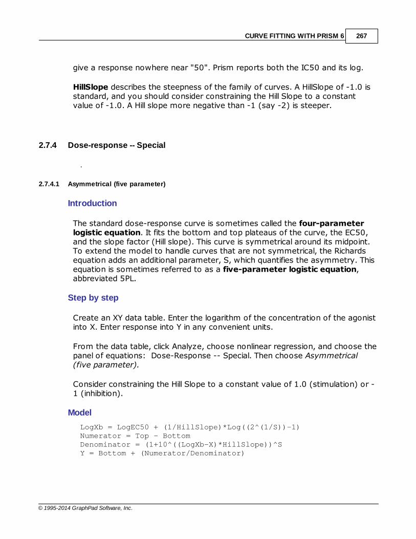
CURVE FITTING WITH PRISM 6 267
© 1995-2014 GraphPad Software, Inc.
give a response nowhere near "50". Prism reports both the IC50 and its log.
HillSlope describes the steepness of the family of curves. A HillSlope of -1.0 isstandard, and you should consider constraining the Hill Slope to a constantvalue of -1.0. A Hill slope more negative than -1 (say -2) is steeper.
2.7.4 Dose-response -- Special
.
2.7.4.1 Asymmetrical (five parameter)
Introduction
The standard dose-response curve is sometimes called the four-parameterlogistic equation. It fits the bottom and top plateaus of the curve, the EC50,and the slope factor (Hill slope). This curve is symmetrical around its midpoint.To extend the model to handle curves that are not symmetrical, the Richardsequation adds an additional parameter, S, which quantifies the asymmetry. Thisequation is sometimes referred to as a five-parameter logistic equation,abbreviated 5PL.
Step by step
Create an XY data table. Enter the logarithm of the concentration of the agonistinto X. Enter response into Y in any convenient units.
From the data table, click Analyze, choose nonlinear regression, and choose thepanel of equations: Dose-Response -- Special. Then choose Asymmetrical(five parameter).
Consider constraining the Hill Slope to a constant value of 1.0 (stimulation) or -1 (inhibition).
Model
LogXb = LogEC50 + (1/HillSlope)*Log((2^(1/S))-1)Numerator = Top - BottomDenominator = (1+10^((LogXb-X)*HillSlope))^SY = Bottom + (Numerator/Denominator)

GraphPad Curve Fitting Guide268
© 1995-2014 GraphPad Software, Inc.
Interpret the parameters
Bottom and Top are the plateaus at the left and right ends of the curve, in thesame units as Y.
LogEC50 is the concentrations that give half-maximal effects, in the sameunits as X. Note that the logEC50 is not the same as the inflection point Xb (seebelow).
HillSlope is the unitless slope factor or Hill slope. Consider constraining it toequal 1.0 (stimulation) or -1 (inhibition).
S is the unitless symmetry parameter. If S=1, the curve is symmetrical andidentical to the standard dose-response equation. If S is distinct than 1.0, thenthe curve is asymmetric as shown below.

CURVE FITTING WITH PRISM 6 269
© 1995-2014 GraphPad Software, Inc.
-10 -9 -8 -7 -6 -5 -4 -30
50
100
0.5 1 2S =
Log [X]
Re
sp
on
se
Notes
The inflection point is called LogXb. It is not the same as the logEC50. Using thebuilt in equation, Prism does not fit logXb, but you can do so using thisequation:
1/Sb 50
1LogX =LogEC + Log 2 -1
HillSlope
You can rewrite the equation so Prism fits the logXb rather than the logEC50. Clone the built-in equation, and edit the copy. Remove the first line [LogXb =
LogEC50 + (1/HillSlope)*Log((2^(1/S))-1)] from the equation. Then
establish a rule for the initial value of the logXb to be 1 * (Value of X atYmid).
Reference
Girlado et al. (Pharmacol. Ther., 95, 21-45, 2002)
2.7.4.2 Equation: Biphasic dose-response
Introduction
A common deviation from the standard monotonic sigmoid shape is thebiphasic sigmoid shape.
Step by step
Create an XY data table. Enter the logarithm of the concentration of the agonistinto X. Enter response into Y in any convenient units.
From the data table, click Analyze, choose nonlinear regression, and choose the
409
433
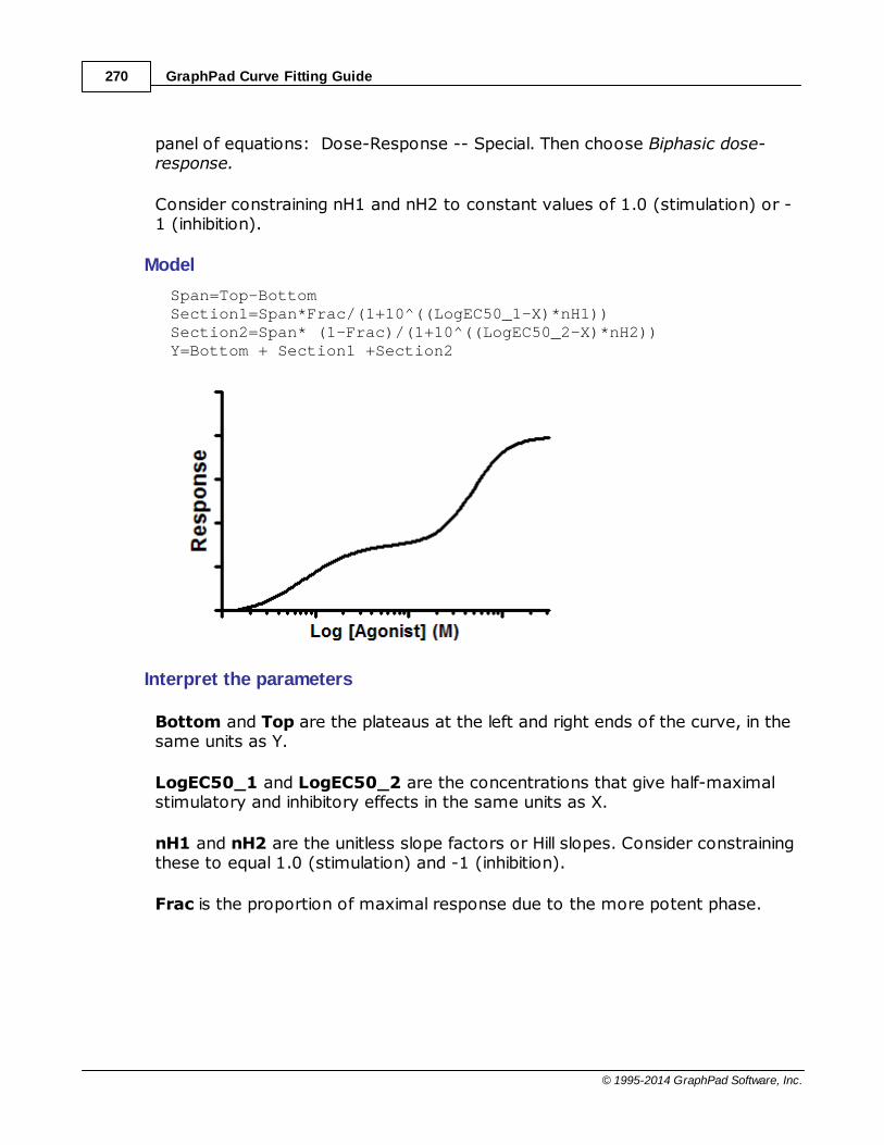
GraphPad Curve Fitting Guide270
© 1995-2014 GraphPad Software, Inc.
panel of equations: Dose-Response -- Special. Then choose Biphasic dose-response.
Consider constraining nH1 and nH2 to constant values of 1.0 (stimulation) or -1 (inhibition).
Model
Span=Top-BottomSection1=Span*Frac/(1+10^((LogEC50_1-X)*nH1))Section2=Span* (1-Frac)/(1+10^((LogEC50_2-X)*nH2))Y=Bottom + Section1 +Section2
Interpret the parameters
Bottom and Top are the plateaus at the left and right ends of the curve, in thesame units as Y.
LogEC50_1 and LogEC50_2 are the concentrations that give half-maximalstimulatory and inhibitory effects in the same units as X.
nH1 and nH2 are the unitless slope factors or Hill slopes. Consider constrainingthese to equal 1.0 (stimulation) and -1 (inhibition).
Frac is the proportion of maximal response due to the more potent phase.

CURVE FITTING WITH PRISM 6 271
© 1995-2014 GraphPad Software, Inc.
2.7.4.3 Equation: Bell-shaped dose-response
Introduction
Some drugs may cause an inhibitory response at low concentrations, and astimulatory response at high concentrations, or vice-versa. The net result is abell-shaped dose-response curve.
The model explained here is the sum of two dose-response curves, one thatstimulates and one that inhibits. you will need lots of data to determine all theparameters without ambiguity, so this model will rarely be useful for dataanalysis. But it might be useful as a way to draw a smooth curve through thedata
Step by step
Create an XY data table. Enter the logarithm of the concentration of the agonistinto X. Enter response into Y in any convenient units.
From the data table, click Analyze, choose nonlinear regression, and choose thepanel of equations: Dose-Response -- Special. Then choose Bell-shaped dose-response.
Consider constraining nH1 and nH2 to constant values of 1.0 (stimulation) and-1 (inhibition).
Model
Span1=Plateau1-DipSpan2=Plateau2-DipSection1=Span1/(1+10^((LogEC50_1-X)*nH1))Section2=Span2/(1+10^((X-LogEC50_2)*nH2))Y=Dip+Section1+Section2

GraphPad Curve Fitting Guide272
© 1995-2014 GraphPad Software, Inc.
Interpret the parameters
Plateau1 and Plateau2 are the plateaus at the left and right ends of the curve,in the same units as Y.
Dip is the plateau level in the middle of the curve, in same units as Y. Note thatwhen the curve goes up first (then down), this parameter named Dip wouldbetter be named Peak.
LogEC50_1 and LogEC50_2 are the concentrations that give half-maximalstimulatory and inhibitory effects in the same units as X.
nH1 and nH2 are the unitless slope factors or Hill slopes. Consider constrainingthese to equal 1.0 (stimulation) and -1 (inhibition).
2.7.4.4 Equation: Operational model - Depletion
Introduction to the operational model
The EC50 is determined by two properties of the agonist:
How well it binds to the receptor, quantified by the affinity of the drug for
binding to its receptor.
How well it causes a response once bound. This property is known as the
CURVE FITTING WITH PRISM 6 273
© 1995-2014 GraphPad Software, Inc.
agonist’s efficacy. Since efficacy depends on both agonist and tissue, asingle drug acting on a single kind of receptor can have different efficacies,and thus different EC50 values, in different tissues.
A single dose-response experiment cannot determine affinity and efficacy. Adrug that binds with high affinity but has low efficacy will produce exactly thesame dose-response curve as a drug with low affinity and high efficacy.
To untangle affinity from efficacy, globally fit a dose-response curve of a fullagonist and a second dose-response curve determined after treating the cellsor tissue with an alkylating agent (or some other irreversible treatment) thatreduces the number of accessible receptors. With fewer receptors, the doseresponse curve is shifted down and usually to the right.
The operational model assumes that the affinity of the drug for the receptors isnot altered by reducing the number of available receptors. It also assumes thatthe maximum possible response in the tissue remains unchanged (thetreatment was specific for the receptors you are studying). Accepting theseassumptions, fitting the operational model globally will determine the affinity ofthe agonist for the receptors.
Step by step
Create an XY data table. Enter the logarithm of the concentration of the agonistligand into X. Enter response into Y in any convenient units. Enter data with afull agonist and no receptor depletion into column A. Enter data collected afterreceptor depletion into column B. Repeat, if you have data with different levelsof receptor depletion for column C, D, E, ... You don't have to know the degreeto which the receptors are depleted, and don't have to enter any values in thecolumn titles (although they are useful as labels).
From the data table, click Analyze, choose nonlinear regression, and choose thepanel of equations: Dose-Response -- Special. Then choose Operational Model- Depletion.
If you have subtracted off any basal response, consider constraining theparameter Basal to a constant value of zero.
Also consider constraining the transducer slope n to a constant value of 1.0.When set to 1.0, all dose-response curves are constrained to have Hill slopes of1.0, which is observed commonly.
Model
operate= (((10^logKA)+(10^X))/(10^(logtau+X)))^nY=Basal + (Effectmax-Basal)/(1+operate)

GraphPad Curve Fitting Guide274
© 1995-2014 GraphPad Software, Inc.
Interpret the parameters
Effectmax is the maximum possible system response, in units of the Y axis. Itis the top plateau of the dose-response curve obtained with a full agonistwithout receptor depletion. If your agonist isn't a full agonist, the EffectMaxmight be higher than the top plateau of the no depletion curve.
Basal is the response in absence of agonist, in same units as Y. If you havesubtracted off any basal response, constrain basal to a constant value of zero.
KA is the agonist-receptor dissociation constant, in same units as X (usuallymolar). It measures the affinity of the full agonist for the receptors, which is themain goal of this kind of experiment. Prism reports both KA and its logarithm. Itis not the same as the EC50.
tau is the transducer constant, a practical measure of efficacy. It is the inverseof the fraction of receptors that must be occupied by agonist to obtain the half-maximal response. If tau equals 10, that means that occupation of only 10% ofthe receptors leads to a half-maximal response. If tau equals 1.0, that meansthat it requires occupation of all the receptors to give a half-maximal response.This would happen in a tissue where the receptors had been substantiallydepleted. Because t is a property of both the tissue and receptor system, it isnot a direct measure of intrinsic efficacy, which is commonly defined as aproperty belonging only to an agonist-receptor pair, irrespective of the assaysystem in which it is measured. Prism reports both tau and its logarithm foreach data set.
n is the Unitless transducer slope. It is similar to, but not identical to, the Hillslope. In most cases, n is constrained to a constant value of 1.0, in which case

CURVE FITTING WITH PRISM 6 275
© 1995-2014 GraphPad Software, Inc.
all the dose-response curves will have Hill slopes of 1.0. If n does not equal 1.0,the Hill Slope does not equal either 1.0 or n.
Notes
Since Tau measures efficacy, Prism fits a different value of tau for each dataset. Receptor depletion reduce the value of tau. The other parameters are fitglobally, to find one best-fit value for all the data sets.
Reference
Black and Leff (Proc. R. Soc. Lond. B, 220: 141-162, 1983
2.7.4.5 Equation: Operational model - Partial agonist
Introduction to the operational model
The EC50, fit by standard dose-response models, is determined by twoproperties of the agonist:
How well it binds to the receptor, quantified by the affinity of the drug for
binding to its receptor.
How well it causes a response once bound. This property is known as the
agonist’s efficacy. Since efficacy depends on both agonist and tissue, asingle drug acting on a single kind of receptor can have different efficacies,and thus different EC50 values, in different tissues.
A single dose-response experiment cannot determine affinity and efficacy. Adrug that binds tightly with high affinity but has low efficacy, will produce exactlythe same dose-response curve as a drug with low affinity and high efficacy.
To determine the affinity of a partial agonist, use the operational model toglobally fit the dose-response curves of both a full agonist and the partialagonist. The data from the full-agonist determines the maximum possibleeffect. Knowing that, the fitting can determine the affinity of the partial agonist.
Step by step
Create an XY data table. Enter the logarithm of the concentration of the agonistligand into X. Enter response into Y in any convenient units. Enter data with thefull agonist into column A. Enter data collected with a partial agonist into columnB. Repeat, if you have data with different partial agonists, for column C, D,E, ..., each with a different amount of depletion.

GraphPad Curve Fitting Guide276
© 1995-2014 GraphPad Software, Inc.
From the data table, click Analyze, choose nonlinear regression, and choose thepanel of equations: Dose-Response -- Special. Then choose Operational Model- Partial agonists.
If you have subtracted off any basal response, consider constraining theparameter Basal to a constant value of zero.
Also consider constraining the transducer slope n to a constant value of 1.0.When set to 1.0, all dose-response curves are constrained to have Hill slopes of1.0, which is observed commonly. If n is not 1.0, the Hill slopes will not be 1.0,but the Hill slopes will not equal exactly n.
Model
operate= (((10^logKA)+(10^X))/(10^(logtau+X)))^n<A> Y = Basal + (Effectmax-Basal)/(1+10^((LogEC50-X)*n))<~A> Y = Basal + (Effectmax-Basal)/(1+operate)
The second line is preceded with <A> which means it only applies to the firstdata set. It fits a variable slope dose-response curve. The third line is precededwith <~A> which means it applies to all data set except the first. It fits theoperational model to determine the affinity (KA) of the partial agonist.
Interpret the parameters
Effectmax is the maximum possible system response, in units of the Y axis. Itis the top plateau of the full agonist's dose-response curve.
Basal is the response in absence of agonist, in same units as Y. If you havesubtracted off any basal response, constrain basal to a constant value of zero.

CURVE FITTING WITH PRISM 6 277
© 1995-2014 GraphPad Software, Inc.
KA is the equilibrium dissociation constant of the partial agonist(s), in sameunits as X (usually molar). It measures the affinity of the partial agonist for thereceptors, which is the main goal of this kind of experiment. Prism reports bothKA and its logarithm. It is not the same as the EC50.
tau is the transducer constant, a practical measure of efficacy. It is the inverseof the fraction of receptors that must be occupied by agonist to obtain the half-maximal response. If t equals 10, that means that occupation of only 10% ofthe receptors leads to a half-maximal response. If t equals 1.0, that means thatit requires occupation of all the receptors to give a half-maximal response. Thiswould happen with a partial agonist. Prism reports both tau and its logarithm,and fits tau individually for each data set.
n is the Unitless transducer slope. It is similar to, but not identical to, the Hillslope. In most cases, n is constrained to a constant value of 1.0, in which caseall the dose-response curves will have Hill slopes of 1.0. If n does not equal 1.0,the Hill Slope does not equal either 1.0 or n.
Reference
Black and Leff (Proc. R. Soc. Lond. B, 220: 141-162, 1983
2.7.4.6 Equation: Gaddum/Schild EC50 shift
Introduction
A competitive inhibitor competes for agonist binding to a receptor, and shiftsthe dose-response curve to the right without changing the maximum response.By fitting all the curves globally, you can determine the affinity of thecompetitive inhibitor.
Step by step
Create an XY data table. Enter the logarithm of the concentration of the agonistligand into X. Enter response into Y in any convenient units. Enter data with noinhibitor into column A. Enter data collected with a constant concentration ofinhibitor into column B. Repeat, if you have data, for column C, D, E, ..., eachwith a different concentration of inhibitor. Enter the inhibitor concentration (inmolar so 1nM is entered as '1e-9') into the column titles. Don't forget to enter'0' as the column title for data set A.
From the data table, click Analyze, choose nonlinear regression, and choose thepanel of equations: Dose-Response -- Special. Then choose Gaddum/SchildEC50 shift.

GraphPad Curve Fitting Guide278
© 1995-2014 GraphPad Software, Inc.
Consider constraining the parameters HillSlope and SchildSlope to their standardvalues of 1.0. This is especially useful if you don't have many data points, andtherefore cannot fit these parameters.
Model
EC50=10^LogEC50Antag=1+(B/(10^(-1*pA2)))^SchildSlopeLogEC=Log(EC50*Antag)Y=Bottom + (Top-Bottom)/(1+10^((LogEC-X)*HillSlope))
Interpret the parameters
EC50 is the concentration of agonist that gives half maximal response in theabsence of inhibitor. Prism reports both the EC50 and its log.
pA2 is the negative logarithm of the concentration of antagonist needed toshift the dose response curve by a factor of 2. If the HillSlope and SchildSlopeare fixed to 1.0, it is the pKb, the negative log of the equilibrium dissociationconstant (Molar) of inhibitors binding to the receptors.
HillSlope describes the steepness of the family of curves. A HillSlope of 1.0 isstandard, and you should consider constraining the Hill Slope to a constantvalue of 1.0.
SchildSlope quantifies how well the shifts correspond to the prediction ofcompetitive interaction. If the competitor is competitive, the SchildSlope will

CURVE FITTING WITH PRISM 6 279
© 1995-2014 GraphPad Software, Inc.
equal 1.0. You should consider constraining SchildSlope to a constant value of1.0. antagonist term, [B], is now raised to the power S, where S denotes theSchild slope factor. If the shift to the right is greater than predicted bycompetitive interactions, S will be greater than 1. If the rightward shift is lessthan predicted by competitive interaction, then S will be less than 1.
Top and Bottom are plateaus in the units of the Y axis.
When is the Schild model valid?
Colquhoun (1) has shown that the Schild model is valid whenever you canmake these assumptions:
The antagonist, B, is a true antagonist that, alone, does not change the
conformation of the receptor.
Binding of agonist, A, and antagonist, B, is mutually exclusive at every
binding site.
B has the same affinity for every binding site.
The observed response is the same if the occupancy of each site by A is the
same, regardless of how many sites are occupied by B.
Measurements are made at equilibrium.
1. Colquhoun, D.. Why the Schild method is better than Schild realised. TrendsPharmacol Sci (2007) vol. 28 (12) pp. 608-14
2.7.4.7 Equation: EC50 shift
Introduction
An competitive inhibitor competes for agonist binding to a receptor, and shiftsthe dose-response curve to the right without changing the maximum response.This model fits the two dose response curves and determines the fold shift.

GraphPad Curve Fitting Guide280
© 1995-2014 GraphPad Software, Inc.
Step by step
Create an XY data table. Enter the logarithm of the concentration of the agonistligand into X. Enter response into Y in any convenient units. Enter data with noinhibitor into column A. Enter data collected with a constant concentration ofinhibitor into column B.
From the data table, click Analyze, choose nonlinear regression, and choose thepanel of equations: Dose-Response -- Special. Then choose Dose shift.
If you have subtracted off any basal signal, constrain the parameter Bottom toa constant value of zero.
Model
<A>LogEC=LogEC50Control<~A>LogEC=LogEC50Control + log(EC50Ratio)Y=Bottom + (Top-Bottom)/(1+10^((LogEC-X)*HillSlope))
EC50Control is the concentration of agonist that gives half maximal responsein the absence of modulator.
Top and Bottom are plateaus in the units of the Y axis (shared).
EC50Ratio is the ratio of EC50 in presence of inhibitor divided by EC50 ofagonist alone.
HillSlope is the slope factor (shared)

CURVE FITTING WITH PRISM 6 281
© 1995-2014 GraphPad Software, Inc.
Notes
If you have several concentrations of antagonist, use a different model that
will directly fit the Schild model and determine the pA2.
2.7.4.8 Equation: Allosteric EC50 shift
Introduction
An allosteric modulator can reduce or enhance agonist binding. This model fitsentire dose-response curves determined in the absence and presence of amodulator. The goal is to learn the affinity of the modulator for binding to itssite, and also determine the value of alpha, the ternary complex constant thatquantifies the degree to which binding of the modulator alters the affinity of theradioligand for the receptor site.
Step by step
Create an XY data table. Enter the logarithm of the concentration of the agonistligand into X. Enter response into Y in any convenient units. Enter data with nomodulator into column A. Enter data collected with a constant concentration ofmodulator into column B. Repeat, if you have data, for column C, D, E, ..., eachwith a different concentration of modulator. Enter the modulator concentration(in molar so 1nM is entered as '1e-9') into the column titles. Don't forget toenter '0' as the column title for data set A.
From the data table, click Analyze, choose nonlinear regression, and choose thepanel of equations: Dose-Response -- Special. Then choose Allosteric EC50shift.
You do not need to constrain any parameters to constant values
Model
EC50=10^LogEC50KB=10^LogKBalpha=10^LogalphaAntag=(1+B/KB)/(1+alpha*B/KB)LogEC=Log(EC50*Antag)Y=Bottom+(Top-Bottom)/(1+10^((LogEC-X)*HillSlope))
277

GraphPad Curve Fitting Guide282
© 1995-2014 GraphPad Software, Inc.
EC50 is the concentration of agonist that gives half maximal response in theabsence of modulator.
Kb is the equilibrium dissociation constant (Molar) of modulator binding to itsallosteric site. It is in the same molar units used to enter the modulatorconcentration into column titles on the data table.
Alpha is the ternary complex constant. When alpha=1.0, the modulator won'talter binding. If alpha is less than 1.0, then the modulator reduces ligand binding.If alpha is greater than 1.0, then the modulator increases binding. In theexample shown about, alpha equals 0.01 so the modulator greatly decreasesbinding.
Top and Bottom are plateaus in the units of the Y axis.
Notes
This model is designed to analyze data when the modulator works via an
allosteric site. Since the agonist and modulator are acting via different sites,it is incorrect to refer to the modulator as a competitor.
The model is written to fit the logarithm of alpha, rather than alpha itself.
This is because alpha is asymmetrical: All values from 0 to 1 mean that themodulator decreases binding, while all values from 1 to infinity mean thatthe modulator enhances binding. On a log scale, its values are moresymmetrical, so the confidence interval computed on a log scale (as Prismdoes) are more accurate. Prism reports both alpha and log(alpha).

CURVE FITTING WITH PRISM 6 283
© 1995-2014 GraphPad Software, Inc.
This model assumes that the allosteric modulator is present in excess, so
the concentration you added is very close to its free concentration. Thismodel won't work when the concentration of allosteric modulator is limiting(as it is when G proteins alter agonist binding to many receptors). Noexplicit model can handle this situation. You need to define the model withan implicit equation (Y on both sides of the equals sign) and Prism cannothandle such equations.
Note two important points about the progression of curves from left to
right with increasing concentrations of the allosteric modulator. First, notethat the maximum response doesn't change. Second, note that the effectof the modulator to right-shift the dose-response curve reaches amaximum as the modulator saturates its binding site.
Reference
A. Christopoulos and T. Kenakin, Pharmacol Rev, 54: 323-374, 2002
2.7.4.9 Equation: ECanything
Introduction
Many log(dose) response curves follow the familiar symmetrical sigmoidalshape. The usual goal is to determine the EC50 of the agonist - theconcentration that provokes a response half way between the basal (Bottom)response and the maximal (Top) response. But you can determine any spotalong the curve, say a EC80 or EC90.
Many dose-response curves have a standard slope of 1.0. This model does notassume a standard slope but rather fits the Hill Slope from the data. Hence thename Variable slope model. This is preferable when you have plenty of datapoints.
Step by step
Create an XY data table. Enter the logarithm of the concentration of the agonistinto X. Enter response into Y in any convenient units. Enter one data set intocolumn A, and use columns B, C... for different treatments, if needed.
From the data table, click Analyze, choose nonlinear regression, and choose thepanel of equations: Dose-Response -- Special. Then choose "log(Agonist) vs.response -- Find ECanything".
You must constrain the parameter F to have a constant value between 0 and100. Set F to 80 if you want to fit the EC80. If you constrain F to equal 50,

GraphPad Curve Fitting Guide284
© 1995-2014 GraphPad Software, Inc.
then this equation is the same as a variable slope dose-response curve.
Consider constraining the parameter HillSlope to its standard value of 1.0 of -1.This is especially useful if you don't have many data points, and thereforecannot fit the slope very well.
If you have subtracted off any basal response, consider constraining Bottom toa constant value of 0.
Model
logEC50=logECF - (1/HillSlope)*log(F/(100-F))Y=Bottom + (Top-Bottom)/(1+10^((LogEC50-X)*HillSlope))
Interpret the parameters
ECf is the concentration of agonist that gives a response F percent of the waybetween Bottom and Top. Prism reports both the ECF and its log.
HillSlope describes the steepness of the family of curves. A HillSlope of 1.0 isstandard, and you should consider constraining the Hill Slope to a constantvalue of 1.0. A Hill slope greater than 1.0 is steeper, and a Hill slope less than1.0 is shallower.
Top and Bottom are plateaus in the units of the Y axis.
ICanything
This equation can also fit inhibitory data where the curve goes downhill ratherthan uphill. The best-fit value of the Hill Slope will be negative in this case.Theresult will always be reported as ECf. Let's say you set F=80. Then the ECf forinhibitory data would be the concentration (X value) required to bring the curve

CURVE FITTING WITH PRISM 6 285
© 1995-2014 GraphPad Software, Inc.
down to 80%. If you want the concentration that brings the curve down by80%, to 20%, then you'd need to set F equal to 20.
2.7.5 Receptor binding - Key concepts
2.7.5.1 Law of mass action
What is the law of mass action?
Analysis of radioligand binding experiments is based on a simple model, calledthe law of mass action. This model assumes that binding is reversible.
Binding occurs when ligand and receptor collide due to diffusion, and when thecollision has the correct orientation and enough energy. The rate of associationis:
Number of binding events per unit of time =[Ligand] [Receptor] kon.
Once binding has occurred, the ligand and receptor remain bound together for arandom amount of time. The probability of dissociation is the same at everyinstant of time. The receptor doesn't "know" how long it has been bound to theligand. The rate of dissociation is:
Number of dissociation events per unit time = [ligand×receptor]×koff.
After dissociation, the ligand and receptor are the same as at they were beforebinding. If either the ligand or receptor is chemically modified, then the bindingdoes not follow the law of mass action.
Equilibrium is reached when the rate at which new ligand×receptor complexesare formed equals the rate at which the ligand×receptor complexes dissociate.At equilibrium:

GraphPad Curve Fitting Guide286
© 1995-2014 GraphPad Software, Inc.
Meaning of Kd
Rearrange that equation to define the equilibrium dissociation constant Kd.
The Kd has a meaning that is easy to understand. Set [Ligand] equal to Kd inthe equation above. The Kd terms cancel out, and you will see that [Receptor]/[Ligand×Receptor]=1, so [Receptor] equals [Ligand×Receptor]. Since all thereceptors are either free or bound to ligand, this means that half the receptorsare free and half are bound to ligand. In other words, when the concentration ofligand equals the Kd, half the receptors will be occupied at equilibrium. If thereceptors have a high affinity for the ligand, the Kd will be low, as it will take alow concentration of ligand to bind half the receptors.
The term "dissociation constant"
Don't mix up Kd, the equilibrium dissociation constant, with koff, thedissociation rate constant. They are not the same, and aren't even expressed inthe same units.
Variable Name Units
kon Association rate constant or on-rateconstant
M-1 min-1
koff Dissociation rate constant or off-rateconstant
min-1
Kd Equilibrium dissociation constant M
Fractional occupancy
The law of mass action predicts the fractional receptor occupancy at equilibriumas a function of ligand concentration. Fractional occupancy is the fraction of allreceptors that are bound to ligand.
This equation is not useful, because you don't know the concentration ofunoccupied receptor, [Receptor]. A bit of algebra creates a useful equation.

CURVE FITTING WITH PRISM 6 287
© 1995-2014 GraphPad Software, Inc.
This equation assumes equilibrium. To make sense of it, think about a fewdifferent values for [Ligand].
[Ligand] Fractional Occupancy
0 0%
1.Kd 50%
4.Kd 80%
9.Kd 90%
99.Kd 99%
Note that when [Ligand]=Kd, fractional occupancy is 50%.
Assumptions
Although termed a "law", the law of mass action is simply a model that can beused to explain some experimental data. Because it is so simple, the model isnot useful in all situations. The model assumes:
All receptors are equally accessible to ligands.
Receptors are either free or bound to ligand. It doesn't allow for more than
one affinity state, or states of partial binding.
Binding does not alter the ligand or receptor.
Binding is reversible.
Despite its simplicity, the law of mass action has proven to be very useful indescribing many aspects of receptor pharmacology and physiology.

GraphPad Curve Fitting Guide288
© 1995-2014 GraphPad Software, Inc.
2.7.5.2 Nonspecific binding
In addition to binding to receptors of interest, radioligands also bind to othersites. Binding to the receptor of interest is called specific binding, while binding tothe other sites is called nonspecific binding. This means that nonspecific bindingcan represent several phenomena:
In most cases, the bulk of nonspecific binding represents some sort of
interaction of the ligand with membranes. The molecular details are unclear,but nonspecific binding depends on the charge and hydrophobicity of a ligand– but not its exact structure.
Nonspecific binding can also be binding to receptors, transporters, or other
proteins not of interest to the investigator. For example binding of theadrenoceptor agonist, epinephrine, to serotonin receptors or metabolicenzymes can be considered “nonspecific”.
Nonspecific binding can also be binding to the filters used to separate bound
from free ligand.
Nonspecific binding is usually (but not necessarily) proportional to theconcentration of radioligand (within the range it is used). Add twice as muchradioligand, and you will see twice as much nonspecific binding.
Nonspecific binding is detected by measuring radioligand binding in the presenceof a saturating concentration of an unlabeled drug that binds to the receptors.Under those conditions, virtually all the receptors are occupied by the unlabeleddrug so the radioligand can only bind to nonspecific sites. Subtract thenonspecific binding at a particular concentration of radioligand from the totalbinding at that concentration to calculate the specific radioligand binding toreceptors.
Which unlabeled drug should you use for determining nonspecific binding? Theobvious answer is to use the same compound as the radioligand, but in itsunlabeled form. In many cases this is necessary, as no other drug is known tobind to the receptors. But most investigators avoid using the same compoundas the hot and cold ligand and prefer to define nonspecific binding with a drugthat is chemically distinct from the radioligand but which binds to the samereceptor.
What concentration of unlabeled drug should you use? You want to use enoughto block virtually all the specific radioligand binding, but not so much that youcause more general physical changes to the membrane that might alter binding.If you are studying a well-characterized receptor, a useful rule-of-thumb is touse the unlabeled compound at a concentration equal to 100 times its Kd forthe receptors, or 100 times the highest concentration of radioligand, whichever

CURVE FITTING WITH PRISM 6 289
© 1995-2014 GraphPad Software, Inc.
is higher.
Ideally, you should get the same results defining nonspecific binding with arange of concentrations of several drugs, and you should test this whenpossible. In many assay systems, nonspecific binding is only 10-20% of thetotal radioligand binding. If the nonspecific binding makes up more than half ofthe total binding, you will find it hard to get quality data. If your system has alot of nonspecific binding, try different kinds of filters, a larger volume ofwashing buffer, warmer washing buffer, or a different radioligand.
2.7.5.3 Ligand depletion
In many experimental situations, you can assume that a very small fraction ofthe ligand binds to receptors (or to nonspecific sites). In these situations, youcan also assume that the free concentration of ligand is approximately equal tothe concentration you added. This assumption vastly simplifies the analysis ofbinding experiments, and the standard analysis methods depend on thisassumption.
In other situations, a large fraction of the ligand binds to the receptors (or bindsnonspecifically). This means that the concentration of ligand free in the solutiondoes not equal the concentration you added. The discrepancy is not the samein all tubes or at all times. The free ligand concentration is depleted by binding.
Many investigators use this rule of thumb: If less than 10% of the ligand binds,don't worry about ligand depletion; if more than 10% of the ligand binds, youhave three choices:
Change the experimental conditions. Increase the reaction volume without
changing the amount of tissue. The problem with this approach is that itrequires more radioligand, which is usually very expensive.
Measure the free concentration of ligand in every tube. This is possible if you
use centrifugation or equilibrium dialysis, but is quite difficult if you usevacuum filtration to remove free radioligand.
Use analysis techniques that adjust for the difference between the
concentration of added ligand and the concentration of free ligand. Prismincludes such models for analyzing saturation and competition data.These special analyses only work with radioactive ligands, so theassessment of added ligand and bound ligand are in the same counts-per-minute units. These methods don't work with fluorescent ligands.
295 318

GraphPad Curve Fitting Guide290
© 1995-2014 GraphPad Software, Inc.
2.7.5.4 The radioactivity web calculator
GraphPad Software provides a free radioactivity calculator on graphpad.com.Use it to perform seven common calculations.
Calculation Description
Isotope decay Calculates radioactive decay during a specifiednumber of days. Select one of the common isotopes,or enter the half-life of another isotope.
Conc. of stock Enter mCi/ml and Ci/mmole, which should be on thelabel. If you are using a molecule labeled with 125I,the specific activity equals 2200 Ci/mmole if eachmolecule is labeled with one iodine.
Also enter the percent of the original isotoperemaining (calculated above). The calculationsassume that the decay product is not biologicallyactive, so the concentration of stock that isbiologically active decreases over time.
Dilution ofstock
Enter the concentration in your stock solution, afteraccounting for decay. Also enter the concentrationand volume you want. The result is the volume ofstock you need to use.
Specific activity(cpm/fmol)
Enter the specific radioactivity as Ci/mmol whichshould be on the label. If you are using a moleculelabeled with 125I, the specific activity equals 2200 Ci/mmol if each molecule is labeled with one iodine.
Also enter the counter efficiency - the fraction ofradioactive disintegrations that are detected. Theefficiency depends on the isotope andinstrumentation. With low energy isotopes such astritium, the efficiency also depends on theexperimental details such as the choice of scintillationfluid, the amount of water in the sample, and thepresence of any colored substances in the sample.
Cpm to fmol/mg
Enter the specific radioactivity as cpm/fmol, thenumber of cpm counted, and the protein content ofthe sample in mg. The result is the number of bindingsites in fmol/mg protein.

CURVE FITTING WITH PRISM 6 291
© 1995-2014 GraphPad Software, Inc.
Calculation Description
Cpm to sites/cell
Enter the specific radioactivity as cpm/fmol, thenumber of cpm counted, and the cell count. The resultis the number of binding sites per cell.
Cpm to nM Enter the specific radioactivity as cpm/fmol, thenumber of cpm counted, and the volume counted.The result is the concentration of radioligand in nM.
2.7.6 Receptor binding - Saturation binding
2.7.6.1 Key concepts: Saturation binding
What is saturation binding?
In a saturation binding experiment, you vary the concentration of radioligandand measure binding at equilibrium. The goal is to determine the Kd (ligandconcentration that binds to half the receptor sites at equilibrium) and Bmax(maximum number of binding sites).
Total, nonspecific and specific binding
The ligand binds not only to receptors sites, but also to nonspecific sites. Thereare three approaches to dealing with nonspecific binding.
Subtract off the nonspecific, and analyze only the specific binding .
Analyze the total binding only , inferring the amount of nonspecific binding
from the shape of the total binding curve.
Globally fit total and nonspecific binding together .
We recommend the third approach (global fitting of total and nonspecific). Theproblem with fitting specific binding is that you have to make someassumptions in order to subtract nonspecific from total, and the resulting valuesthat you fit aren't really data. When possible, we suggest that you fit the datayou actually collect, and avoid creating derived data sets (specific binding, in thiscase).
Fitting total binding only requires less data, so saves experimental time andmoney. But most people feel unconformable defining nonspecific binding purely
297
292
293
GraphPad Curve Fitting Guide292
© 1995-2014 GraphPad Software, Inc.
from the shape of a binding curve, without experimentally measuringnonspecific binding. One advantage of fitting total binding only is that equationshave been derived for fitting such data, even when a substantial fraction of theligand binds, resulting in ligand depletion (free concentration substantially lessthan the added concentration).
One-vs. two sites
Prism offers models for fitting one or two sites. You can use choices in theCompare tab to compare the two fits. When comparing the fits to the one- andtwo-site models, use common sense as well as statistics. Don't accept a twosite model, if one of the sites is only a tiny fraction of the total, or if its Kd isoutside the range of radioligand concentrations you used in the experiment.
2.7.6.2 Equation: One site -- Total binding
Introduction
You don't have to measure nonspecific binding directly. Instead, you candetermine Bmax and Kd by fitting only total binding by assuming that theamount of nonspecific binding is proportional to the concentration ofradioligand.
Step by step
Create an XY data table. Enter radioligand concentration into X, and totalbinding into Y. If you have several experimental conditions, place the first intocolumn A, the second into column B, etc.
Use any convenient units for X and Y. The Kd will be reported in the same unitsas X, and the Bmax will be reported in the same units as Y.
From the table of total binding, click Analyze, choose nonlinear regression,choose the panel of Saturation Binding equations, and choose One site -- Total.
Consider constraining the parameter Background to a constant value of zero.This is the measured 'binding' when there is no radioligand binding added, sorepresents the counter background, if there is any.
Model
Y=Bmax*X/(Kd+X) + NS*X + Background
295

CURVE FITTING WITH PRISM 6 293
© 1995-2014 GraphPad Software, Inc.
Interpret the parameters
Bmax is the maximum specific binding in the same units as Y.
Kd is the equilibrium binding constant, in the same units as X. It is theradioligand concentration needed to achieve a half-maximum binding atequilibrium.
NS is the slope of nonspecific binding in Y units divided by X units.
Background is the amount of nonspecific binding with no added radioligand.This represents counter background. If your counter automatically subtracts offthe background signal, you can constrain Background to a constant value ofzero.
Notes
This analysis assumes that only a small fraction of radioligand binds, whichmeans that the concentration you added is virtually identical to the freeconcentration. If you can't make this assumption, use an alternative analysis .
2.7.6.3 Equation: One site -- Fit total and nonspecific binding
Introduction
In a saturation binding experiment, you vary the concentration of radioligandand measure binding. The goal is to determine the Kd (ligand concentration thatbinds to half the receptor sites at equilibrium) and Bmax (maximum number ofbinding sites).
The ligand binds not only to receptors sites, but also to nonspecific sites. There
295

GraphPad Curve Fitting Guide294
© 1995-2014 GraphPad Software, Inc.
are three approaches to dealing with nonspecific binding.
Subtract off the nonspecific, and analyze only the specific binding .
Analyze the total binding only, inferring the amount of nonspecific binding
from the shape of the total binding curve. Learn more .
Globally analyze the total and nonspecific binding at one time. This is the
best approach, and the details are explained below.
Step by step
Create an XY data table. Enter radioligand concentration into X, total bindinginto Y, and nonspecific binding into column B.
Use any convenient units for X. The Kd will be reported in those sameconcentration units. Use the same units for total and nonspecific binding. TheBmax will be reported in those same units.
Alternatively choose the sample data set: Binding - Saturation binding to totaland nonspecific.
From the data table, click Analyze, choose nonlinear regression, choose thepanel of Saturation Binding equations, and choose One site -- Total andnonspecific binding.
Consider constraining the parameter Background to a constant value of zero.This is the measured 'binding' when there is no radioligand binding added, sorepresents the counter background, if there is any.
Model
specific=Bmax*X/(X+Kd)nonspecific=NS*X + Background<A>Y=specific+nonspecific<B>Y=nonspecific
The <A> and <B> syntax means that the third line is only used for data set A(total binding) while the fourth line is used only for data set B (nonspecific).
The parameters NS and Background are shared between the two data sets.
297
292
41

CURVE FITTING WITH PRISM 6 295
© 1995-2014 GraphPad Software, Inc.
Interpret the parameters
Bmax is the maximum specific binding in the same units as Y. It is the specificbinding extrapolated to very high concentrations of radioligand, so it value is isalmost always higher than any specific binding measured in your experiment.
Kd is the equilibrium binding constant, in the same units as X. It is theradioligand concentration needed to achieve a half-maximum binding atequilibrium.
NS is the slope of nonspecific binding in Y units divided by X units.
Background is the amount of nonspecific binding with no added radioligand.This represents counter background. If your counter automatically subtracts offthe background signal, you can constrain Background to a constant value ofzero.
2.7.6.4 Equation: One site -- Total, accounting for ligand depletion
Introduction
You don't have to measure nonspecific binding directly. Instead, you candetermine Bmax and Kd by fitting only total binding by assuming that theamount of nonspecific binding is proportional to the concentration ofradioligand.
If only a small fraction of radioligand binds, you can use a simpler model .292

GraphPad Curve Fitting Guide296
© 1995-2014 GraphPad Software, Inc.
This equation allows for a substantial fraction of the added ligand to bind. Thisonly works with radioactive ligands, so the assessment of added ligand andbound ligand are in the same counts-per-minute units. This method doesn'twork with fluorescent ligands.
Step by step
Create an XY data table. Enter radioligand concentration into X, and totalbinding into Y. If you have several experimental conditions, place the first intocolumn A, the second into column B, etc.
Enter both X and Y in CPM units. This is essential for the analysis to work.
From the table of total binding, click Analyze, choose nonlinear regression,choose the panel of Saturation Binding equations, and choose One site -- Total,accounting for ligand depletion.
You must constrain two parameters to constant values based on yourexperimental design:
SpAct is the specific radioactivity in cpm/fmol
Vol is the reaction volume in ml
Model
KdCPM=KdnM * Vol * 1000 * SpecAct ; (nm/L * mL * 0.001 L/ml * 1000000 fmol/nmol * cpm/fmol)a=-1-NSb=KdCPM + NS*KdCPM + X + 2*X*NS + Bmaxc=-1*X*(NS*KdCPM + X*NS+Bmax)Y=(-b+sqrt(b*b-4*a*c) )/(2*a) ;Y is in cpm

CURVE FITTING WITH PRISM 6 297
© 1995-2014 GraphPad Software, Inc.
Interpret the parameters
Bmax is the maximum specific binding in cpm.
KdnM is the equilibrium binding constant in nM. It is the radioligandconcentration needed to achieve a half-maximum specific binding at equilibrium.
NS is the slope of nonspecific binding in Y units divided by X units.
Notes
This analysis accounts for the fact that a large fraction of the added radioligandbinds to the receptors. If you are able to assume that only a small fraction ofradioligand binds, which means that the concentration you added is virtuallyidentical to the free concentration, use an alternative analysis .
Reference
This equation came from S. Swillens (Molecular Pharmacology, 47: 1197-1203, 1995)
2.7.6.5 Equation: One site -- Specific binding
Introduction
In a saturation binding experiment, you vary the concentration of radioligandand measure binding. The goal is to determine the Kd (ligand concentration thatbinds to half the receptor sites at equilibrium) and Bmax (maximum number ofbinding sites).
The ligand binds not only to receptors sites, but also to nonspecific sites. Thereare three approaches to dealing with nonspecific binding.
Subtract off the nonspecific, and analyze only the specific binding. Read on
for this approach.
Analyze the total binding only, inferring the amount of nonspecific binding
from the shape of the total binding curve. Learn more .
Globally analyze the total and nonspecific binding at one time. Learn more.
Step by step
Create an XY data table. Enter radioligand concentration into X, and specific
292
292
293

GraphPad Curve Fitting Guide298
© 1995-2014 GraphPad Software, Inc.
binding into Y. If you have several experimental conditions, place the first intocolumn A, the second into column B, etc.
An alternative approach would be to enter total binding into column A, andnonspecific into column B. Then use the Remove Baseline analysis to subtractcolumn B from column A, creating a new results table with the specific binding.
From the table of specific binding, click Analyze, choose nonlinear regression,choose the panel of Saturation Binding equations, and choose One site specificbinding.
Model
Y = Bmax*X/(Kd + X)
Interpret the parameters
Bmax is the maximum specific binding in the same units as Y. It is the specificbinding extrapolated to very high concentrations of radioligand, and so its valueis almost always higher than any specific binding measured in your experiment.
Kd is the equilibrium binding constant, in the same units as X. It is theradioligand concentration needed to achieve a half-maximum binding atequilibrium.
Create a Scatchard plot
Before nonlinear regression was available, investigators had to transformcurved data into straight lines, so they could analyze with linear regression. Oneway to do this is with a Scatchard plot, which plots specific binding vs. the ratioof specific binding to the concentration of free radioligand.
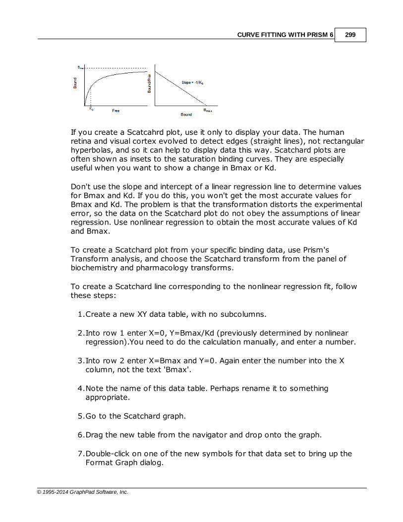
CURVE FITTING WITH PRISM 6 299
© 1995-2014 GraphPad Software, Inc.
If you create a Scatcahrd plot, use it only to display your data. The humanretina and visual cortex evolved to detect edges (straight lines), not rectangularhyperbolas, and so it can help to display data this way. Scatchard plots areoften shown as insets to the saturation binding curves. They are especiallyuseful when you want to show a change in Bmax or Kd.
Don't use the slope and intercept of a linear regression line to determine valuesfor Bmax and Kd. If you do this, you won't get the most accurate values forBmax and Kd. The problem is that the transformation distorts the experimentalerror, so the data on the Scatchard plot do not obey the assumptions of linearregression. Use nonlinear regression to obtain the most accurate values of Kdand Bmax.
To create a Scatchard plot from your specific binding data, use Prism'sTransform analysis, and choose the Scatchard transform from the panel ofbiochemistry and pharmacology transforms.
To create a Scatchard line corresponding to the nonlinear regression fit, followthese steps:
1.Create a new XY data table, with no subcolumns.
2.Into row 1 enter X=0, Y=Bmax/Kd (previously determined by nonlinearregression).You need to do the calculation manually, and enter a number.
3.Into row 2 enter X=Bmax and Y=0. Again enter the number into the Xcolumn, not the text 'Bmax'.
4.Note the name of this data table. Perhaps rename it to somethingappropriate.
5.Go to the Scatchard graph.
6.Drag the new table from the navigator and drop onto the graph.
7.Double-click on one of the new symbols for that data set to bring up theFormat Graph dialog.

GraphPad Curve Fitting Guide300
© 1995-2014 GraphPad Software, Inc.
8.Choose to plot no symbols, but to connect with a line.
Notes
This is not the best way to determine Bmax and Kd. It is better to globally
fit total and nonspecific binding , without subtracting to compute specificbinding.
When making a Scatchard plot, you have to choose what units you want to
use for the Y-axis. Some investigators express both free ligand and specificbinding in cpm so the ratio bound/free is a unitless fraction. While this iseasy to interpret (it is the fraction of radioligand bound to receptors), analternative is to express specific binding in sites/cell or fmol/mg protein, andto express the free radioligand concentration in nM. While this makes the Y-axis hard to interpret visually, it provides correct units for the slope (whichequals -1/Kd).
2.7.6.6 Equation: One site -- Specific binding with Hill slope
Introduction
In a saturation binding experiment, you vary the concentration of radioligandand measure binding. The goal is to determine the Kd (ligand concentration thatbinds to half the receptor sites at equilibrium) and Bmax (maximum number ofbinding sites).
This equation assumes you have subtracted off the nonspecific, and are onlyanalyzing specific binding.
This equation fits a Hill slope. If you assume the Hill slope is 1.0 (for massaction binding of a monomer to one site) use a simpler equation .
Step by step
Create an XY data table. Enter radioligand concentration into X, and specificbinding into Y. If you have several experimental conditions, place the first intocolumn A, the second into column B, etc.
An alternative approach would be to enter total binding into column A, andnonspecific into column B. Then use the Remove Baseline analysis to subtractcolumn B from column A, creating a new results table with the specific binding.
From the table of specific binding, click Analyze, choose nonlinear regression,
293
297

CURVE FITTING WITH PRISM 6 301
© 1995-2014 GraphPad Software, Inc.
choose the panel of Saturation Binding equations, and choose One site specificbinding with Hill Slope.
Model
Y=Bmax*X^h/(Kd^h + X^h)
Note that the X axis is concentration, not log(concentration).
Interpret the parameters
Bmax is the maximum specific binding in the same units as Y. It is the specificbinding extrapolated to very high concentrations of radioligand, and so its valueis almost always. higher than any specific binding measured in yourexperiment.
Kd is the radioligand concentration needed to achieve a half-maximum bindingat equilibrium, expressed in the same units as X. If h=1.0, this is the equilibriumbinding constant. If h is not equal to 1.0, then the molecular interpretation ofthe Kd depends on why h is not 1.0.
h is the Hill slope. It equals 1.0 when a monomer binds with no cooperativity toone site. When it is greater than 1.0, you see a sigmoidal look to the graph asshown above. This happens when the receptor or ligand has multiple bindingsites with positive cooperativity. The Hill slope is less than zero when there aremultiple binding sites with different affinities for ligand or when there is negativecooperativity.

GraphPad Curve Fitting Guide302
© 1995-2014 GraphPad Software, Inc.
2.7.6.7 Binding potential
The problem: Binding isotherms without going to high enoughconcentrations
The figure above shows a saturation binding equation fit to specific binding data.But all the concentrations are relatively low (compared to the Kd of binding) sothe data almost form a straight line. The saturation binding model fits the datafine (solid curve), with a narrow 95% confidence band around the curve(dashed lines). But look at the confidence interval for Bmax and Kd (shown inthe box)! They are super wide, even descending into negative (impossible)values. With these data, the curve fit the data fine, but neither parameter in themodel (Bmax and Kd) were fit with reasonable confidence intervals. This is nosurprise. The data don’t show even a hint of plateauing, so the data simplydon’t define the Bmax and Kd at all.
The problem is that the data are consistent with a system with a huge numberof low affinity receptors (high Bmax; high Kd) or a smaller number of highaffinity receptors (low Bmax; low Kd). The figure below shows two ways thevisualize this. The graph on the left shows the same fit as the one above, butwith the best-fit curve and its confidence bands extended out to largerconcentrations. While the confidence band is tight near the points, is it superwide as it goes beyond concentrations with data. The graph on the right showtwo different fits, with the Kd constrained to equal 200 nM or 500 nM. Thecurves are very different, yet both go near the data.

CURVE FITTING WITH PRISM 6 303
© 1995-2014 GraphPad Software, Inc.
Another way to look at the problem with these data is that the Bmax and Kdare correlated. Prism can report the covariance matrix as part of its nonlinearregression results. With only two parameters, there is only one value in that"matrix". The covariance between Kd and Bmax (which can range from 0.0 to1.0) is 0.9993. Prism can also report the dependency of each parameter(which also can range from 0.0 to 1.0). With only two parameters, both havethe same dependency, which is 0.9986 for this example. This is not quite highenough for Prism to declare the results ambiguous, but the threshold for thatdesignation (dependency > 0.9999) is arbitrary.
It is tempting to give up at this point and say that nothing can be determinedwithout more data at higher concentrations. But in some systems, especiallythose using PET scanning to detect receptors, data like this are typical. It isimpossible to use higher concentrations of ligand.
Fitting the binding potential
What can be learned from these data? The data are nearly linear. What doesthe slope of that line tell us? The slope, or rather the initial slope, is termed the binding potential (1). Don’t be mislead by the term potential. It has nothing todo with potential energy and thermodynamics. Rather it is a measure of howmuch binding will occur with a small amount of ligand.
If you start with the specific binding equation, take its derivative with respect toX (which is concentration), and set X equal to zero, you’ll derive the initial slopeof a specific binding curve. It turns out that this slope, the binding potential,equals Bmax/Kd. Bmax is measured in the same units as the Y values in thedata. Kd is measured in the same units as the X values. So the binding potentialhas units equal to the Y units divided by the X units.
Prism can fit a specific binding curve, and also report the ratio of Bmax/Kd withits confidence interval. To do this either create a new user-defined equation or(easier) clone the built in one. Then go to the last tab of the dialog that defines

GraphPad Curve Fitting Guide304
© 1995-2014 GraphPad Software, Inc.
the equation. “Transforms to Report”. Choose to report the ratio of twoparameters, and define the numerator and denominator.
In this example, Prism finds that the Binding Potential is 242.1, with aconfidence interval ranging from 183.4 to 300.7. That confidence interval isreasonably narrow, so the result is quite useful.
Reference
1. Innis et al. Consensus nomenclature for in vivo imaging of reversibly bindingradioligands. Journal of Cerebral Blood Flow & Metabolism (2007) vol. 27 (9)pp. 1533-1539
Download the Prism file for this example.
2.7.6.8 Equation: Two sites -- Specific binding only
Introduction
In a saturation binding experiment, you vary the concentration of radioligandand measure binding. The goal is to determine the Kd (ligand concentration thatbinds to half the receptor sites at equilibrium) and Bmax (maximum number ofbinding sites) of both kinds of receptors.

CURVE FITTING WITH PRISM 6 305
© 1995-2014 GraphPad Software, Inc.
The ligand binds not only to receptors sites, but also to nonspecific sites. Thereare three approaches to dealing with nonspecific binding.
Subtract off the nonspecific, and analyze only the specific binding. Read on
for this approach.
Analyze the total binding only, inferring the amount of nonspecific binding
from the shape of the total binding curve. This approach doesn't work wellwhen there are two classes of receptors.
Globally analyze the total and nonspecific binding at one time. Learn more.
Step by step
Create an XY data table. Enter radioligand concentration into X, and specificbinding into Y. If you have several experimental conditions, place the first intocolumn A, the second into column B, etc.
An alternative approach would be to enter total binding into column A, andnonspecific into column B. Then use the Remove Baseline analysis to subtractcolumn B from column A, creating a new results table with the specific binding.
From the table of specific binding, click Analyze, choose nonlinear regression,choose the panel of Saturation Binding equations, and choose Two sites --Specific binding.
Model
Site1=BmaxHi*X/(KdHi+X)Site2=BmaxLo*X/(KdLo+X)Y=Site1 + Site2
307

GraphPad Curve Fitting Guide306
© 1995-2014 GraphPad Software, Inc.
Interpret the parameters
BmaxHi and BmaxLo are the maximum specific bindings to the two sites inthe same units as Y.
KdHi and KdLo are the equilibrium binding constants, in the same units as X. Itis the radioligand concentration needed to achieve a half-maximum binding atequilibrium
Scatchard plots of two site binding
The left panel below shows binding of a radioligand to two independent bindingsites present in equal concentrations, but with a tenfold difference in Kd . Thetwo individual curves are shown as dotted and dashed curves. When you do theexperiment, you can't observe the individual components, but observe thesum, which is shown as a solid curve. Note that this curve is not obviouslybiphasic.
The right panel shows the same data plotted on a Scatchard plot. The bindingto each receptor is shown as a straight line (dotted, or dashed). The totalbinding, plotted on a Scatchard plot, is curved. Note that the two lines thatrepresent binding to each type of receptor are NOT the asymptotes of thecurve.

CURVE FITTING WITH PRISM 6 307
© 1995-2014 GraphPad Software, Inc.
To plot the two straight lines that correspond to the nonlinear regression fit,create a new data table that defines the two lines as shown below, using Bmaxand Kd values determined by nonlinear regression.
X A B
0 Bmax1/Kd1
Bmax1 0
0 Bmax2/Kd2
Bmax2 0
Go to the graph of the Scatchard transformed data and drag the new table tothat graph. Use the Format Graph dialog to plot the two data sets from thetable using connecting lines but no symbols.
2.7.6.9 Equation: Two sites -- Fit total and nonspecific binding
Introduction
In a saturation binding experiment, you vary the concentration of radioligandand measure binding. The goal is to determine the Kd (ligand concentration thatbinds to half the receptor sites at equilibrium) and Bmax (maximum number ofbinding sites).
The ligand binds not only to receptors sites, but also to nonspecific sites. Thereare three approaches to dealing with nonspecific binding.
Subtract off the nonspecific, and analyze only the specific binding .
Analyze the total binding only, inferring the amount of nonspecific binding
from the shape of the total binding curve. This approach doesn't work wellwhen the ligand binds to two sites
Globally analyze the total and nonspecific binding at one time. This is the
best approach, and the details are explained below.
304

GraphPad Curve Fitting Guide308
© 1995-2014 GraphPad Software, Inc.
Step by step
Create an XY data table. Enter radioligand concentration into X, total bindinginto Y, and nonspecific binding into column B.
Use any convenient units for X. The Kd will be reported in those sameconcentration units. Use the same units for total and nonspecific binding. TheBmax will be reported in those same units.
From the data table, click Analyze, choose nonlinear regression, choose thepanel of Saturation Binding equations, and choose Two sites -- Total andnonspecific binding.
The parameter Background is the measured 'binding' when there is noradioligand binding added, so represents the counter background, if there is any.Consider constraining it to a constant value of zero.
Model
Specific1=BmaxHi*X/(X+KdHi)Specific2=BmaxLo*X/(X+KdLo)Nonspecific=NS*X + Background<A>Y=Specific1 + Specific2 + Nonspecific<B>Y=Nonspecific
The <A> and <B> syntax means that the fourth line is only used for data set A(total binding) while the fifth line is used only for data set B (nonspecific).
The parameters NS and Background are shared between the two data sets.
Interpret the parameters
BmaxHi and BmaxLo are the maximum specific bindings to the two sites inthe same units as Y.
KdHi and KdLo are the equilibrium binding constants, in the same units as X. Itis the radioligand concentration needed to achieve a half-maximum binding atequilibrium.
NS is the slope of nonspecific binding in Y units divided by X units.
Background is the amount of nonspecific binding with no added radioligand.This represents counter background. If your counter automatically subtracts offthe background signal, you can constrain Background to a constant value ofzero.

CURVE FITTING WITH PRISM 6 309
© 1995-2014 GraphPad Software, Inc.
2.7.6.10 Equation: One site with allosteric modulator
Introduction
An allosteric modulator can reduce radioligand binding. This model fitsexperiments, where entire radioligand binding curves are measured in theabsence and presence of modulator. The goal is to learn the affinity of themodulator for binding to its site, and also determine the value of alpha, theternary complex constant that quantifies the degree to which binding of themodulator alters the affinity of the radioligand for the receptor site.
Step by step
Create an XY data table. Enter the concentration of the labeled ligand into X,using any convenient units (maybe nM). Enter specific binding into Y in anyconvenient units. Enter data with no modulator into column A. Enter datacollected with a constant concentration of modulator into column B. Repeat, ifyou have data, for column C, D, E, ..., each with a different concentration ofmodulator. Enter the modulator concentration (in nanomolar so 1nM is enteredas '1') into the column titles. Don't forget to enter '0' as the column title fordata set A.
From the data table, click Analyze, choose nonlinear regression, choose thepanel of Saturation Binding equations, and choose Allosteric modulator shift.
You don't need to constrain any parameters to constant values.
Model
Hot=XAlpha=10^logalphaKB=10^logKBKApp=KDHot*((1+Allo/KB)/(1+alpha*Allo/KB))Y=Bmax*Hot/(Hot+KApp)

GraphPad Curve Fitting Guide310
© 1995-2014 GraphPad Software, Inc.
Interpret the parameters
Kb is the equilibrium dissociation constant (Molar) of modulator binding to itsallosteric site. It is in the same molar units used to enter the modulatorconcentration into column titles on the data table.
KdHot is the equilibrium dissociation constant of the radioligand. It is expressedin the same units used to enter X values, nM in the example.
Alpha is the ternary complex constant. When alpha=1.0, the modulator won'talter binding. If alpha is less than 1.0, then the modulator reduces ligand binding.If alpha is greater than 1.0, then the modulator increases binding. In theexample shown about, alpha equals 0.01 so the modulator greatly decreasesbinding.
Notes
This model is designed to analyze data when the unlabeled compound
works via an allosteric site. Since the labeled and unlabeled ligands areacting via different sites, it is inappropriate (and incorrect) to refer to themodulator as a competitor.
The model is written to fit the logarithm of alpha, rather than alpha itself.
This is because alpha is asymmetrically (all values from 0 to 1 mean thatthe modulator decreases binding, while all values from 1 to infinity meanthat the modulator enhances binding. On a log scale, its values are moresymmetrical, so the confidence interval computed on a log scale (as Prismdoes) are more accurate. Prism reports both alpha and log(alpha).
This model assumes that the allosteric modulator is present in excess, so

CURVE FITTING WITH PRISM 6 311
© 1995-2014 GraphPad Software, Inc.
the concentration you added is very close to its free concentration. Thismodel won't work when the concentration of allosteric modulator is limiting(as it is when G proteins alter agonist binding to many receptors). Noexplicit model can handle this situation. You need to define the model withan implicit equation (Y on both sides of the equals sign) and Prism cannothandle such equations.
Reference
A. Christopoulos and T. Kenakin, Pharmacol Rev, 54: 323-374, 2002
2.7.7 Receptor binding - Competitive binding
2.7.7.1 Key concepts: Competitive binding
What is competitive binding?
In a competitive binding experiment, you use a single concentration of labeled(hot) ligand and vary the concentration of unlabeled (cold) drugs, and measurebinding at equilibrium.
Comparing one- and two-site models
Prism offers models for fitting one or two sites. You can use choices in theCompare tab to compare the two fits. When comparing the fits to the one- andtwo-site models, use common sense as well as statistics. Don't accept a twosite model, if one of the sites is only a tiny fraction of the total, or if its Ki isoutside the range of competitor concentrations you used in the experiment.
Ligand depletion
If a large fraction of the added radioligand binds to the receptors, the ligand isdepleted so the concentration you added is greater than the free concentration.You need to fit these data to a model that accounts for ligand depletion .
Homologous binding
An homologous binding experiment is one where the labeled and unlabeledligands have identical affinities for the receptors. Generally this is because thetwo are chemically identical. Receptor number and affinity are determined byanalyzing the competition of varying concentrations of unlabeled ligand for one(or better, two) concentrations of labeled ligand. Prism offers a special model
318

GraphPad Curve Fitting Guide312
© 1995-2014 GraphPad Software, Inc.
for fitting homologous competition experiments .
Allosteric modulators
Allosteric modulators can alter radioligand binding, even though they bind todifferent sites. Since the hot and cold ligands bind to different sites, the term'competition' is not apt, but we include this model here because theexperimental design is the same as used for competitive binding. Prism can fitbinding inhibition (or augmentation) by an allosteric modulator based on theternary complex model. Note that this model assumes the allosteric modulatoris present in excess, so is not depleted by binding to the receptors.
2.7.7.2 Equation: One site - Fit Ki
Introduction
You can determine the equilibrium dissociation constant of an unlabelled ligandby measuring its competition for radioligand binding.
Step by step
Create an XY data table. Enter the logarithm of the concentration of theunlabeled compound into X, and binding into Y. If you have several experimentalconditions, place the first into column A, the second into column B, etc. Usesubcolumns to enter replicates.
From the data table, click Analyze, choose nonlinear regression, choose thepanel of Competition Binding equations, and choose One site - Fit Ki.
You must constrain two parameters to constant values based on yourexperimental design:
RadioligandNM is the concentration of labeled ligand in nM. A single
concentration of radioligand is used for the entire experiment.
HotKdNM is the equilibrium dissociation constant of the labeled ligand in nM.
Model
logEC50=log(10^logKi*(1+RadioligandNM/HotKdNM))Y=Bottom + (Top-Bottom)/(1+10^(X-LogEC50))
321
322

CURVE FITTING WITH PRISM 6 313
© 1995-2014 GraphPad Software, Inc.
Interpret the parameters
Top and Bottom are plateaus in the units of Y axis.
logKI is the log of the molar equilibrium dissociation constant of unlabeledligand.
Ki is the equilibrium dissociation constant in Molar.
Notes
This model fits the Ki of the unlabelled ligand directly. It does not report theEC50, so you do not need to apply the Cheng and Prusoff correction(1).Instead you enter the concentration of radioligand and its Kd as constants, andPrism directly fits the Ki of your cold compound. If you want to know the IC50,fit a log(dose)-response curve.
If you want to know the IC50 (which is not very informative in this situation) fitthe data using an alternative equation .
The analysis assumes that you have one site, and that the binding is reversibleand at equilibrium.
1. Cheng, Y. and Prusoff, W. H. Relationship between the inhibition constant (K1) and theconcentration of inhibitor which causes 50 per cent inhibition (I50) of an enzymatic reaction.Biochem Pharmacol, 22: 3099-3108, 1973.
314

GraphPad Curve Fitting Guide314
© 1995-2014 GraphPad Software, Inc.
2.7.7.3 Equation: One site - Fit logIC50
Introduction
You can determine the equilibrium dissociation constant of an unlabelled ligandby measuring its competition for radioligand binding.
Step by step
Create an XY data table. Enter the logarithm of the concentration of theunlabeled compound into X, and binding into Y. If you have several experimentalconditions, place the first into column A, the second into column B, etc. Usesubcolumns to enter replicates.
From the data table, click Analyze, choose nonlinear regression, choose thepanel of Competition Binding equations, and choose One site - Fit logEC50.
Model
Y=Bottom + (Top-Bottom)/(1+10^(X-LogIC50))
Interpret the parameters
Top and Bottom are plateaus in the units of Y axis.
logIC50 is the log of the concentration of competitor that results in bindinghalf-way between Bottom and Top

CURVE FITTING WITH PRISM 6 315
© 1995-2014 GraphPad Software, Inc.
Notes
This model is the same as an inhibitory dose-response curve. It fits the logIC50,which is not the same as the Ki of the unlabelled ligand for binding. The Kidepends on the IC50, the concentration of radioligand, and its Kd for binding.You can fit the Ki directly using a different equation .
The analysis assumes that you have one site, and that the binding is reversibleand at equilibrium.
2.7.7.4 Equation: Two sites - Fit Ki
Introduction
You can determine the equilibrium dissociation constant of an unlabelled ligandby measuring its competition for radioligand binding. This model assumes thatthere are two classes of sites with identical affinity for the radioligand, butdifferent affinities for the competitor.
Step by step
Create an XY data table. Enter the logarithm of the concentration of theunlabeled compound into X, and binding into Y. If you have several experimentalconditions, place the first into column A, the second into column B, etc. Usesubcolumns to enter replicates.
From the data table, click Analyze, choose nonlinear regression, choose thepanel of Competition Binding equations, and choose Two sites - Fit Ki.
You must constrain three parameters to constant values based on yourexperimental design:
RadioligandNM is the concentration of labeled ligand in nM. A single
concentration of radioligand is used for the entire experiment.
KdHi is the equilibrium dissociation constant of the labeled ligand for the
high-affinity site in nM.
KdLo is the equilibrium dissociation constant of the labeled ligand for the
low-affinity site in nM.
Model
ColdnM=10^(X+9)
312

GraphPad Curve Fitting Guide316
© 1995-2014 GraphPad Software, Inc.
KIHinM = 10^(LogKI_Hi+9)KILonM = 10^(LogKI_Lo+9)SITE1= HotnM*(Top-Bottom)/(HotnM + KDHotNM_Ki*(1+coldnM/KiHinM))SITE2= HotnM*(Top-Bottom)/(HotnM + KDHotNM_Lo*(1+coldnM/KiLonM))Y = SITE1*FractionHi + SITE2*(1-FractionHi) + Bottom
Interpret the parameters
Top and Bottom are plateaus in the units of Y axis.
FractionHi is the fraction of all the sites that have high affinity for thecompetitor.
logKi_Hi and logKi_Lo are the logarithms of the two molar Ki values.
Notes
This model fits the two log(Ki) values of the unlabelled ligand directly. It doesnot report the IC50s, so you do not need to apply the Cheng and Prusoffcorrection(1). Instead you enter the concentration of radioligand and its Kd asconstants, and Prism directly fits the Ki of your cold compound. If you want tofit the two IC50 values instead of the Ki values, use a different equation .
The analysis assumes that you know the affinity of both sites for the labeledligand. In many cases, the radioligand has the same affinity for both sites. Inthat case, simply enter that value twice. If the two sites have different affinitiesfor the labeled ligand, enter both values (determined from other experiments).Watch out for the labels. The constant KdHi is the Kd of the hot ligand for thereceptors with the high affinity for the unlabeled ligand, and KdLo is the Kd of
317

CURVE FITTING WITH PRISM 6 317
© 1995-2014 GraphPad Software, Inc.
the hot ligand for the receptors with lower affinity for the unlabeled ligand. SoKdHi may be larger or smaller than KdLo.
This analysis assumes that the binding is reversible and at equilibrium. It alsoassumes that the labeled and unlabeled ligands compete for the same bindingsites.
1. Cheng, Y. and Prusoff, W. H. Relationship between the inhibition constant (K1) and theconcentration of inhibitor which causes 50 per cent inhibition (I50) of an enzymatic reaction.Biochem Pharmacol, 22: 3099-3108, 1973.
2.7.7.5 Equation: Two sites - Fit logIC50
Introduction
You can determine the equilibrium dissociation constant of an unlabelled ligandby measuring its competition for radioligand binding. This model assumes thatthere are two classes of sites with identical affinity for the radioligand, butdifferent affinities for the competitor.
Step by step
Create an XY data table. Enter the logarithm of the concentration of theunlabeled compound into X, and binding into Y. If you have several experimentalconditions, place the first into column A, the second into column B, etc. Usesubcolumns to enter replicates.
From the data table, click Analyze, choose nonlinear regression, choose thepanel of Competition Binding equations, and choose Two sites - Fit logIC50.
Model
Span=Top-BottomSection1=Span*FractionHi/(1+10^((X-LogIC50HI)))Section2=Span* (1-FractionHi)/(1+10^((X-LogIC50Lo)))Y=Bottom + Section1 +Section2

GraphPad Curve Fitting Guide318
© 1995-2014 GraphPad Software, Inc.
Interpret the parameters
Top and Bottom are plateaus in the units of Y axis.
FractionHi is the fraction of all the sites that have high affinity for thecompetitor.
logIC50Hi and logIC50Lo are the logarithms of the two IC50 values.
Notes
This model fits the two IC50 values of the unlabelled ligand. It does not reportthe two Ki values. The Ki values depend on the IC50s, the concentration ofradioligand, and its Kd for binding. You can fit the Ki values directly using a different equation .
This analysis assumes that the binding is reversible and at equilibrium. It alsoassumes that the labeled and unlabeled ligands compete for the same bindingsites.
2.7.7.6 Equation: One site - Ligand depletion
Introduction
This model for competitive binding is useful when a large fraction of the addedradioligand binds to the receptors, so the concentration you added is greaterthan the free concentration.
315

CURVE FITTING WITH PRISM 6 319
© 1995-2014 GraphPad Software, Inc.
These equation allows for a substantial fraction of the added ligand to bind. Thisonly works with radioactive ligands, so the assessment of added ligand andbound ligand are in the same counts-per-minute units. This method doesn'twork with fluorescent ligands.
Step by step
Create an XY data table. Enter the logarithm of the molar concentration of theunlabeled compound into X, and binding into Y. The Y values must be in cpm.
If you have several experimental conditions, place the first into column A, thesecond into column B, etc. Use subcolumns to enter replicates.
From the data table, click Analyze, choose nonlinear regression, choose thepanel of Competition Binding equations, and choose One site -- Heterologouswith depletion.
You must constrain four parameters to constant values based on yourexperimental design:
Hot is the amount of labeled ligand in cpm. A single concentration of
radioligand is used for the entire experiment.
KdNM is the equilibrium dissociation constant of the labeled ligand in nM.
SpAct is the specific radioactivity in cpm/fmol.
Vol is the reaction volume in ml.
Model
KdCPM=KdnM*SpAct*vol*1000 ; nmol/L *(cpm/fmol * ml * .001L/ml * 1000000fmol/nmol) = cpmR=NS+1S=[1+10^(X-LogKi)]*KdCPM+Hota=-1*Rb=R*S+NS*Hot + Bmaxc= -1*Hot*(S*NS + Bmax)Y= (-1*b + sqrt(b*b-4*a*c))/(2*a)

GraphPad Curve Fitting Guide320
© 1995-2014 GraphPad Software, Inc.
Interpret the parameters
logKI is the log of the molar equilibrium dissociation constant of unlabeledligand.
Ki is the equilibrium dissociation constant in Molar.
Bmax is the maximum binding of ligand to receptors in cpm. This representsbinding to all the receptors so is higher than the top plateau of the curve.
NS is the fraction of the radioligand that binds to nonspecific sites.
Notes
This analysis accounts for the fact that a large fraction of the added radioligandbinds to the receptors. If you are able to assume that only a small fraction ofradioligand binds, which means that the concentration you added is virtuallyidentical to the free concentration, use an alternative analysis .
Reference
This equation came from S. Swillens (Molecular Pharmacology, 47: 1197-1203, 1995)
312

CURVE FITTING WITH PRISM 6 321
© 1995-2014 GraphPad Software, Inc.
2.7.7.7 Equation: One site - Homologous
Introduction
An homologous binding experiment is one where the labeled and unlabeledligands have identical affinities for the receptors. Generally this is because thetwo are chemically identical. Receptor number and affinity are determined byanalyzing the competition of varying concentrations of unlabeled ligand for one(or better, two) concentrations of labeled ligand.
Step by step
Create an XY data table. Enter the logarithm of the concentration of theunlabeled compound into X, and binding into Y. Enter the concentration oflabeled ligand (in nM) as the column title. You will get better results if you usetwo different concentrations of labeled ligand.
If you have several experimental conditions, place the first into column A, thesecond into column B, etc. Use subcolumns to enter replicates.
From the data table, click Analyze, choose nonlinear regression, choose thepanel of Competition Binding equations, and choose One site - Homologous.
Model
ColdNM=10^(x+9) ;Cold concentration in nMKdNM=10^(logKD+9) ;Kd in nMY=(Bmax*HotnM)/(HotnM + ColdNM + KdNM) + Bottom

GraphPad Curve Fitting Guide322
© 1995-2014 GraphPad Software, Inc.
Interpret the parameters
logKd Log of the equilibrium binding constant. Since the analysis is based on theassumption that labeled and unlabeled ligand bind with identical affinities, thelogKd applies to both forms of the ligand.
Bmax is the maximum binding of ligand to receptors in cpm. This representsbinding to all the receptors so is higher than the top plateau of the curve.
NS is a measure of nonspecific binding. It is the bottom plateau in units of the Yaxis divided by the concentration of the hot ligand in nM. In other words, it isthe fraction of hot ligand that binds nonspecifically.
Prism fits the curves globally to find one shared value for logKd, Bmax and NSfrom all sets of data
Notes
This model assumes that the hot and cold ligand binds identically to thereceptor, and that you use two concentrations of hot ligand (in column A, and B..) and vary cold. It assumes that a small fraction of added ligand binds, so thefree concentration is close to what you added.
2.7.7.8 Equation: Allosteric modulator
Introduction
Fits a curve of "competition" of binding by an allosteric modulator, based on theternary complex model. Note that this model assumes the allosteric modulatoris present in excess, so is not depleted by binding to the receptors. Since itbinds to a different site than the radioligand, the term 'competition' is not apt,but we list it here because the experimental design is the same as used forcompetitive binding.
Step by step
Create an XY data table. Enter the logarithm of the concentration of theunlabeled modulator (in nM) into X, and specific binding into Y in any convenientunits.
From the data table, click Analyze, choose nonlinear regression, choose thepanel of Competition Binding equations, and choose Allosteric modulatortitration.

CURVE FITTING WITH PRISM 6 323
© 1995-2014 GraphPad Software, Inc.
You must constrain two parameters to constant values based on yourexperimental design:
RadioligandNM is the concentration of labeled ligand in nM. A single
concentration of radioligand is used for the entire experiment.
HotKdNM is the equilibrium dissociation constant of the labeled ligand in nM.
Also consider constraining Y0 (radioligand binding in the absence of modulator)to a constant value.
Model
AlloNM=10^(X+9)KbNM=10^(logKb +9)alpha=10^logAlphaKAppNM=HotKDnm*(((1+(AlloNM/KBNM))/(1+alpha*(AlloNM/KBNM))))HotOccupancy = RadioligandNM/(RadioligandNM + HotKDnm)Y=(Y0/HotOccupancy)*(RadioligandNM/(RadioligandNM + KAppNM))
Interpret the parameters
Kb is the equilibrium dissociation constant (Molar) of modulator binding.
Alpha is the ternary complex constant. When alpha=1.0, the modulator doesnot alter binding. If alpha is less than 1.0, then the modulator reduces ligandbinding. If alpha is greater than 1.0, then the modulator increases binding.
Y0 is the radioligand binding in the absence of modulator. Consider constraining

GraphPad Curve Fitting Guide324
© 1995-2014 GraphPad Software, Inc.
this to a constant value.
Notes
This model is designed to analyze data when the unlabeled compound worksvia an allosteric site. Since the labeled and unlabeled ligands are acting viadifferent sites, it is inappropriate (and incorrect) to refer to these types ofexperiments as “competition binding assays”. In some cases, in fact, theallosteric modulator enhances radioligand binding.
The model is written to fit the logarithm of alpha, rather than alpha itself. This isbecause alpha is asymmetrically (all values from 0 to 1 mean that themodulator decreases binding, while all values from 1 to infinity mean that themodulator enhances binding. On a log scale, its values are more symmetrical,so the confidence interval computed on a log scale (as Prism does) are moreaccurate.
The Y axis plots specific binding. Even at very high concentrations of inhibitor,the specific binding does not descend to zero. This is the nature of allostericinhibition. If alpha is very high, then the binding is inhibited almost to zero. Ifalpha is not so high, then the maximum inhibition is more modest. For example,if alpha=3, the maximum inhibition is down to 33%.
This model assumes that the allosteric modulator is present in excess, so theconcentration you added is very close to its free concentration. This modeldoes not apply when the concentration of allosteric modulator is limiting (as it iswhen G proteins alter agonist binding to many receptors). No explicit model canhandle this situation. You need to define the model with an implicit equation (Yon both sides of the equals sign) and Prism cannot handle such equations.
Reference
A. Christopoulos and T. Kenakin, Pharmacol Rev, 54: 323-374, 2002
2.7.8 Receptor binding - Kinetics
Kinetics refers to changes over time. Kineticbinding experiments are used to determine theassociation and dissociation rate constants.

CURVE FITTING WITH PRISM 6 325
© 1995-2014 GraphPad Software, Inc.
2.7.8.1 Key concepts: Kinetics of binding
Law of mass action
Kinetic binding experiments are used to determine the association anddissociation rate constants. All the analyses assume that binding follows the lawof mass action:
At any given time, the rate at which receptor-ligand complexes form isproportional to the radioligand concentration and the number of receptors stillunoccupied. The rate of dissociation is proportional to the concentration ofreceptor-ligand complexes.
Rate of dissociation
A dissociation binding experiment measures the “off rate” for radioliganddissociating from the receptor. Initially ligand and receptor are allowed to bind,perhaps to equilibrium. At that point, you need to block further binding ofradioligand to receptor (by adding an unlabeled drug or by dilution) so you canmeasure the rate of dissociation, which follows a one-phase exponential decaywith a rate constant equal to the rate of radioligand dissociation.
Rate of association
In an association experiment, you add radioligand and measure specific bindingat various times thereafter.
Binding increases over time until it plateaus. This plateau is not the same as theBmax. The plateau in an association experiment depends on the concentrationof radioligand used, while the Bmax is extrapolated to an infinite concentrationof radioligand.
The rate at which binding increases is determined by three factors (as well asexperimental conditions such as pH and temperature):
The association rate constant, kon or k+1. This is what you are trying to
determine.
The concentration of radioligand. If you use more radioligand, the system
equilibrates faster.
The dissociation rate constant, koff or k-1. Some people are surprised to

GraphPad Curve Fitting Guide326
© 1995-2014 GraphPad Software, Inc.
see that the observed rate of association depends in part on thedissociation rate constant. During the incubation, radioligand both binds toand dissociates from receptors. The system reaches equilibrium when thetwo rates are equal. The observed rate of association measures how long ittakes to reach equilibrium. If the radioligand dissociates quickly from thereceptor, equilibrium will be reached faster (but with less binding).
It is not possible, therefore, to fit a simple association experiment to determinethe association rate constant unless you constrain the value of the dissociationrate constant , measure association kinetics with two or more concentrationsof radioligand , or determine the rate of association and dissociation in oneexperiment .
2.7.8.2 Equation: Dissociation kinetics
Introduction
A dissociation binding experiment measures the “off rate” for radioliganddissociating from the receptor. Initially ligand and receptor are allowed to bind,perhaps to equilibrium. At that point, you need to block further binding ofradioligand to receptor so you can measure the rate of dissociation. There areseveral ways to do this:
If the tissue is attached to a surface, you can remove the buffer containing
radioligand and replace with fresh buffer without radioligand.
Spin the suspension and resuspend in fresh buffer.
Add a very high concentration of an unlabeled ligand. If this concentration is
high enough, it will instantly bind to nearly all the unoccupied receptors andthus block binding of the radioligand.
Dilute the incubation by a large factor, at least 100 fold dilution. This will
reduce the concentration of radioligand by that factor. At such a lowconcentration, new binding of radioligand will be negligible. This method isonly practical when you use a fairly low concentration of radioligand so itsconcentration after dilution is far below its Kd for binding.
You then measure binding at various times after that to determine how rapidlythe radioligand falls off the receptors.
Step by step
Create an XY data table. Enter time into X, and total binding into Y. If you have
328
329
331

CURVE FITTING WITH PRISM 6 327
© 1995-2014 GraphPad Software, Inc.
several experimental conditions, place the first into column A, the second intocolumn B, etc.
From the table of specific binding, click Analyze, choose nonlinear regression,choose the panel of Kinetics Binding equations, and choose Dissociation - Onephase exponential decay .
Model
Y=(Y0-NS)*exp(-K*X) + NS
Interpret the parameters
Y0 is the binding at time zero, in the units of the Y axis.
NS is the binding (nonspecific) at infinite times, in the units of the Y axis.
K is the rate constant in inverse units of the X axis. The half-life equals the ln(2)divided by K.
Checking for cooperativity
If the law of mass action applies, binding of a ligand to one binding site does notalter the affinity of another binding site. This also means that dissociation of aligand from one site should not change the dissociation of ligand from othersites. To test this assumption, compare the dissociation rate after initiatingdissociation by infinite dilution with the dissociation rate when initiated byaddition of a large concentration of unlabeled drug. If the radioligand is bound tomultiple noninteracting binding sites, the dissociation will be identical in bothexperimental protocols as shown in the left figure below. Note that the Y axis isshown using a log scale. If there were a single binding site, you would expectthe dissociation data to appear linear on this graph. With two binding sites, thegraph is curved even on a log axis.

GraphPad Curve Fitting Guide328
© 1995-2014 GraphPad Software, Inc.
The right figure shows ideal dissociation data when radioligand is bound tointeracting binding sites with negative cooperativity. The data are differentdepending on how dissociation was initiated. If dissociation is initiated by infinitedilution, the dissociation rate will change over time. The dissociation of someradioligand will leave the remaining ligand bound more tightly. When dissociationis initiated by addition of cold drug, all the receptors are always occupied byligand (some hot, some cold) and dissociation occurs at its maximal unchangingrate.
2.7.8.3 Equation: Association kinetics (one ligand concentration)
Introduction
When you measure the association rate of a radioligand, the rate at which thebinding equilibrates depends not only on the association rate constant and theamount of ligand you used, but also on its dissociation rate constant. (Why? )The only way to fit the association rate constant by analyzing association datafrom one concentration of radioligand, is to constrain the dissociation rateconstant to a value you determined in a different experiment.
Alternative methods of determining an association rate constant are to globallyfit data obtained with multiple radioligand concentrations , or to analyze anexperiment that measuresboth association and dissociation ratesequentially.
Step by step
Create an XY data table. Enter time in minutes into X, and specific binding intoY.
From the table of specific binding, click Analyze, choose nonlinear regression,choose the panel of Kinetics Binding equations, and choose Association kinetics- One conc. of hot.
You must constrain Hotnm ([radioligand] in nM) and Koff (dissociation rateconstant, in inverse minutes) to constant values.
325
329
331

CURVE FITTING WITH PRISM 6 329
© 1995-2014 GraphPad Software, Inc.
Model
Kd=Koff/KonL=Hotnm*1e-9Kob=Kon*L+KoffOccupancy=L/(L+Kd)Ymax=Occupancy*BmaxY=Ymax*(1 - exp(-1*kob*X))
Interpret the parameters
Kon is the association rate constant, in units of M-1 min-1
Kd is the equilibrium binding constant, in Molar, computed as Koff/Kon
Bmax is the maximal binding at equilibrium, extrapolated to maximalradioligand concentration, in the units used to enter the Y values.
Notes
2.7.8.4 Equation: Association kinetics (two ligand concentrations)
Introduction
You cannot determine kon
from an association binding measured at a single
concentration of radioligand. The observed association rate depends on theassociation rate constant, the amount of ligand you used, and its dissociationrate constant. With one concentration of radioligand, the results are ambiguous..
If you perform an association kinetic experiments with multiple radioligandconcentration, you can globally fit the data to the association kinetic model toderive a single best-fit estimate for k
on and one for k
off.
Shown below is an example of an association kinetic experiment conductedusing two concentrations of radioligand. All other conditions (temperature, pH,

GraphPad Curve Fitting Guide330
© 1995-2014 GraphPad Software, Inc.
etc.) were the same for both runs, of course. Times were entered into the Xcolumn, specific binding for one concentration of radioligand were entered intothe first (A) Y column, and binding for the other concentration were enteredinto column B.
Step by step
Create an XY data table. Enter time in minutes into X, and total binding into Y.Enter binding at one concentration of radioligand into the column A, binding atanother concentration into column B, etc. Enter the concentrations, in nM, intothe column titles.
From the table of specific binding, click Analyze, choose nonlinear regression,choose the panel of Kinetics Binding equations, and choose Association - Two ormore conc. of hot.
Model
Kd=Koff/KonL=Hotnm*1e-9Kob=Kon*L+KoffOccupancy=L/(L+Kd)Ymax=Occupancy*BmaxY=Ymax*(1 - exp(-1*kob*X))
Interpret the parameters
Koff is the dissociation rate constant in min-1.
Kon is the association rate constant, in units of M-1 min-1.
Kd is the equilibrium binding constant, in Molar, computed as Koff/Kon
Bmax is the maximal binding at equilibrium, at maximal radioligand

CURVE FITTING WITH PRISM 6 331
© 1995-2014 GraphPad Software, Inc.
concentration, in the units you used to enter Y.
Notes
According to the law of mass action, the ratio of koff to kon is the Kd ofreceptor binding:
Compare the Kd calculated this way (from kinetic experiments) with the Kddetermined from a saturation binding curve. If binding follows the law of massaction, the two Kd values should be indistinguishable.
2.7.8.5 Equation: Association then dissociation
Introduction
You cannot determine the association rate constant by simply observing theassociation of a single concentration of radioligand. The rate at which a ligandreaches equilibrium is determined not only by the association rate constant andthe ligand concentration, but also by the dissociation constant.
One way to determine the association rate constant is to globally fit dataobtained with two different concentrations of radioligand . An alternativeapproach, explained here is to measure association and dissociation in oneexperiment.
Add a radioligand and measure total binding at multiple time points, then atTime0 initiate dissociation (by adding an antagonist or by massive dilution) andthen measure dissociation at various times.
Step by step
Create an XY data table. Enter time in minutes into X, and total binding into Y.
From the table of specific binding, click Analyze, choose nonlinear regression,choose the panel of Kinetics Binding equations, and choose Association thendissociation.
Constrain HotNM ([radioigand in nM] and Time0 (time at which dissociation wasinitiated) to constant values. If you entered specific binding into the Y column,also constrain NS to a constant value of zero.
328
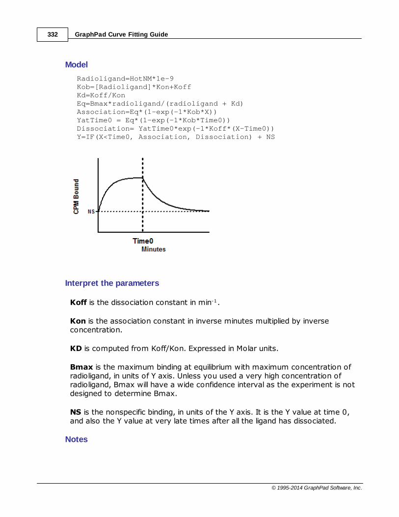
GraphPad Curve Fitting Guide332
© 1995-2014 GraphPad Software, Inc.
Model
Radioligand=HotNM*1e-9Kob=[Radioligand]*Kon+KoffKd=Koff/KonEq=Bmax*radioligand/(radioligand + Kd)Association=Eq*(1-exp(-1*Kob*X))YatTime0 = Eq*(1-exp(-1*Kob*Time0))Dissociation= YatTime0*exp(-1*Koff*(X-Time0))Y=IF(X<Time0, Association, Dissociation) + NS
Interpret the parameters
Koff is the dissociation constant in min-1.
Kon is the association constant in inverse minutes multiplied by inverseconcentration.
KD is computed from Koff/Kon. Expressed in Molar units.
Bmax is the maximum binding at equilibrium with maximum concentration ofradioligand, in units of Y axis. Unless you used a very high concentration ofradioligand, Bmax will have a wide confidence interval as the experiment is notdesigned to determine Bmax.
NS is the nonspecific binding, in units of the Y axis. It is the Y value at time 0,and also the Y value at very late times after all the ligand has dissociated.
Notes
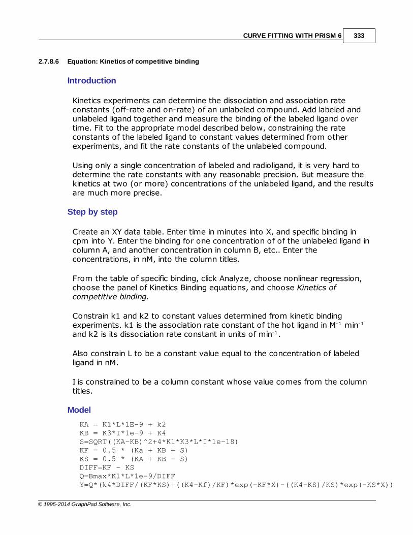
CURVE FITTING WITH PRISM 6 333
© 1995-2014 GraphPad Software, Inc.
2.7.8.6 Equation: Kinetics of competitive binding
Introduction
Kinetics experiments can determine the dissociation and association rateconstants (off-rate and on-rate) of an unlabeled compound. Add labeled andunlabeled ligand together and measure the binding of the labeled ligand overtime. Fit to the appropriate model described below, constraining the rateconstants of the labeled ligand to constant values determined from otherexperiments, and fit the rate constants of the unlabeled compound.
Using only a single concentration of labeled and radioligand, it is very hard todetermine the rate constants with any reasonable precision. But measure thekinetics at two (or more) concentrations of the unlabeled ligand, and the resultsare much more precise.
Step by step
Create an XY data table. Enter time in minutes into X, and specific binding incpm into Y. Enter the binding for one concentration of of the unlabeled ligand incolumn A, and another concentration in column B, etc.. Enter theconcentrations, in nM, into the column titles.
From the table of specific binding, click Analyze, choose nonlinear regression,choose the panel of Kinetics Binding equations, and choose Kinetics ofcompetitive binding.
Constrain k1 and k2 to constant values determined from kinetic bindingexperiments. k1 is the association rate constant of the hot ligand in M-1 min-1
and k2 is its dissociation rate constant in units of min-1.
Also constrain L to be a constant value equal to the concentration of labeledligand in nM.
I is constrained to be a column constant whose value comes from the columntitles.
Model
KA = K1*L*1E-9 + k2KB = K3*I*1e-9 + K4S=SQRT((KA-KB)^2+4*K1*K3*L*I*1e-18)KF = 0.5 * (Ka + KB + S)KS = 0.5 * (KA + KB - S)DIFF=KF - KSQ=Bmax*K1*L*1e-9/DIFFY=Q*(k4*DIFF/(KF*KS)+((K4-Kf)/KF)*exp(-KF*X)-((K4-KS)/KS)*exp(-KS*X))

GraphPad Curve Fitting Guide334
© 1995-2014 GraphPad Software, Inc.
Interpret the parameters
k3 is the association rate constant of unlabeled ligand in M-1 min-1.
k4 is the dissociation rate constant of unlabeled ligand in min-1.
Bmax is the total number of receptors. Either leave as a variable or set to aconstant you know from other experiments. The Bmax is the maximum bindingat equilibrium with a very high concentration of radioligand. It is usually muchlarger than any binding seen in the experiment.
All three parameters are constrained to be shared, so Prism fits one value of each of thethree parameters for all the data sets.
Notes
This equation does not account for ligand depletion. It assumes that only a
small fraction of radioligand binds to receptors, so that the freeconcentration of radioligand is very close to the added concentration.
This method will only give reliable results if you have plenty of data points at
early time points.
The ratio K4/K3 is the equilibrium dissociation constant of the cold ligand in
Molar. You should compare this value (determined via kinetics) with thesame value determined by equilibrium competition.

CURVE FITTING WITH PRISM 6 335
© 1995-2014 GraphPad Software, Inc.
Reference
This method was described by Motulsky and Mahan in Molecular Pharmacology25:1-9, 1984.
2.7.9 Enzyme kinetics -- Key concepts
2.7.9.1 Key concepts: Terminology
What is an enzyme?
Living systems depend on chemical reactions which, on their own, would occurat extremely slow rates. Enzymes are catalysts that reduce the neededactivation energy so these reactions proceed at rates that are useful to the cell.The study of enzyme kinetics can help us understand the function andregulation of enzymes.
Enzyme progress curves
In most cases, an enzyme converts one chemical (the substrate) into another(the product). A graph of product concentration vs. time follows three phasesmarked on the graph below.
Time
[Pro
du
ct]
1.At very early time points (usually less than a second), the rate of productaccumulation increases over time. Special techniques, not available in Prism,are needed to study the early kinetics of enzyme action. The graph aboveexaggerates this first phase.
2.For an extended period of time, the product concentration increases linearlywith time. All the analyses built-in to Prism use data collected during thissecond phase.
3.At later times, the substrate is depleted, so the curve starts to level off.

GraphPad Curve Fitting Guide336
© 1995-2014 GraphPad Software, Inc.
Eventually the concentration of product reaches a plateau.
It is very difficult to fit a curve to these kind of data. The model simply cannotbe reduced to an equation that expresses product concentration as a functionof time. To fit these kind of data (called an enzyme progress curve) you needto use a program that can fit data to a model defined by differential equationsor by an implicit equation. For more details, see RG Duggleby, Analysis ofEnzyme Reaction Progress Curves by Nonlinear Regression, Methods inEnzymology, 249: 61-60, 1995.
Rather than fit the enzyme progress curve, most analyses of enzyme kinetics(including all those built-in to Prism) measure product at a single time point.Analyses assume that the time point you chose is on the linear (second) phaseof product accumulation and ignore the nonlinear first phase (which is usuallyvery short). Therefore, if you divide the amount of product produced by thetime the reaction was allowed to proceed, you compute the amount of productformed per unit time, which is the enzyme velocity.
Terminology
The terminology can be confusing. Note these confusing points:
As mentioned above, almost all studies of enzyme "kinetics" are done by
collecting data at a single time point. The X axis is substrate (or inhibitor)concentration, not time.
The second phase shown in the graph above is often called the "initial
rate", a phrase that makes sense only if you ignore the short transientphase that precedes it.
That second phase is also called "steady state", because the concentration
of enzyme-substrate complex doesn't change during that phase. However,the concentration of product accumulates, so the system is not truly atsteady state until, much later, the concentration of product truly doesn'tchange over time.
2.7.9.2 Key concepts: Assumptions
Standard analyses of enzyme kinetics (the only kind discussed here) assume:
The production of product is linear with time during the time interval used.

CURVE FITTING WITH PRISM 6 337
© 1995-2014 GraphPad Software, Inc.
The concentration of substrate vastly exceeds the concentration of
enzyme. This means that the free concentration of substrate is very closeto the concentration you added, and that substrate concentration isessentially constant throughout the assay.
A single enzyme forms the product.
There is negligible spontaneous creation of product without enzyme.
With the exception of the built-in allosteric model, Prism's built-in equations alsoassume:
No cooperativity. Binding of substrate to one enzyme binding site doesn't
influence the affinity or activity of an adjacent site.
Neither substrate nor product acts as an allosteric modulator to alter the
enzyme velocity.
2.7.10 Enzyme kinetics - Subtrate vs. velocity
2.7.10.1 Key concepts: Substrate vs. velocity
Fitting a substrate-velocity curve
The simplest experiment in enzyme kinetics is to vary the substrateconcentration and measure enzyme velocity.
The standard way to fit these data is to fit the Michaelis-Menten model todetermine the Vmax (maximum enzyme velocity) and its Km (theconcentration of substrate needed to get half-maximal velocity.
The Vmax equals the product of the concentration of active enzyme sites timesthe turnover rate, kcat. This is the number of substrate molecules each enzymesite can convert to product per unit time. If you know the concentration ofenzyme, you can fit the curve to determine kcat and Km . The curve will beidentical to the Michaelis-Menten fit.
If the enzyme has cooperative subunits, the graph of enzyme velocity as afunction of substrate concentration will appear sigmoidal. Prism offers oneempirical equation for fitting sigmoidal substrate-velocity curves .
338
340
342
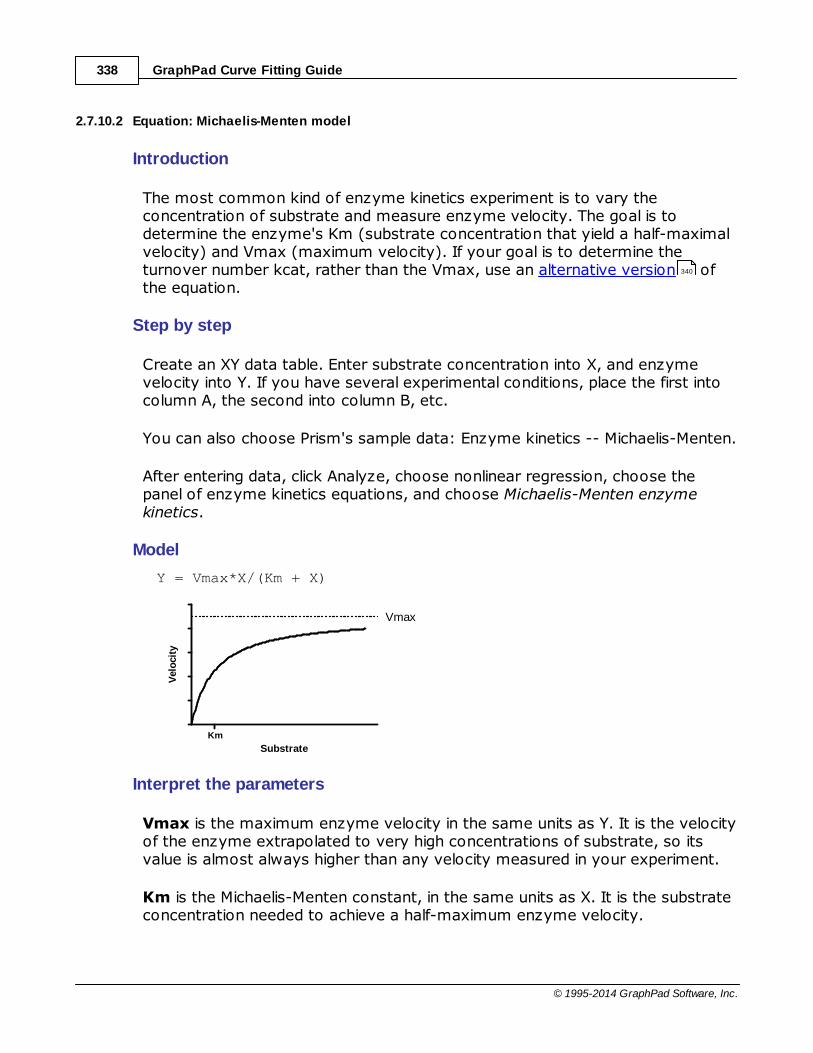
GraphPad Curve Fitting Guide338
© 1995-2014 GraphPad Software, Inc.
2.7.10.2 Equation: Michaelis-Menten model
Introduction
The most common kind of enzyme kinetics experiment is to vary theconcentration of substrate and measure enzyme velocity. The goal is todetermine the enzyme's Km (substrate concentration that yield a half-maximalvelocity) and Vmax (maximum velocity). If your goal is to determine theturnover number kcat, rather than the Vmax, use an alternative version ofthe equation.
Step by step
Create an XY data table. Enter substrate concentration into X, and enzymevelocity into Y. If you have several experimental conditions, place the first intocolumn A, the second into column B, etc.
You can also choose Prism's sample data: Enzyme kinetics -- Michaelis-Menten.
After entering data, click Analyze, choose nonlinear regression, choose thepanel of enzyme kinetics equations, and choose Michaelis-Menten enzymekinetics.
Model
Y = Vmax*X/(Km + X)
Km
Vmax
Substrate
Velo
cit
y
Interpret the parameters
Vmax is the maximum enzyme velocity in the same units as Y. It is the velocityof the enzyme extrapolated to very high concentrations of substrate, so itsvalue is almost always higher than any velocity measured in your experiment.
Km is the Michaelis-Menten constant, in the same units as X. It is the substrateconcentration needed to achieve a half-maximum enzyme velocity.
340

CURVE FITTING WITH PRISM 6 339
© 1995-2014 GraphPad Software, Inc.
Create a Lineweaver-Burk plot
Before nonlinear regression was available, investigators had to transformcurved data into straight lines, so they could analyze with linear regression. Oneway to do this is with a Lineweaver-Burk plot, which plots the reciprocal ofsubstrate concentration vs. the reciprocal of enzyme velocity.
1
Vmax
1
KM
m
max
KSlope=
V
1/[Substrate] 1
/Velo
cit
y
If you create a Lineweaver-Burk plot, use it only to display your data. Don't usethe slope and intercept of a linear regression line to determine values for Vmaxand Km. If you do this, you won't get the most accurate values for Vmax andKm. The problem is that the transformations (reciprocals) distort theexperimental error, so the double-reciprocal plot does not obey theassumptions of linear regression. Use nonlinear regression to obtain the mostaccurate values of Km and Vmax.
To create a Lineweaver-Burk plot with Prism, use the Transform analysis, thenchoose the panel of biochemistry and pharmacology transforms.
To create a Lineweaver-Burke line corresponding to the nonlinear regression fit,follow these steps:
1.Create a new XY data table, with no subcolumns.
2.Into row 1 enter X=-1/KM, Y =0 (previously determined by nonlinearregression).
3.Into row 2 enter X=1/Smin (Smin is the smallest value of [substrate] youwant to include on the graph) and Y=(1/Vmax)(1.0 + KM/Smin).
4.Note the name of this data table. Perhaps rename it to somethingappropriate.
5.Go to the Lineweaver-Burke graph.
6.Drag the new table from the navigator and drop onto the graph.

GraphPad Curve Fitting Guide340
© 1995-2014 GraphPad Software, Inc.
7.Double-click on one of the new symbols for that data set to bring up theFormat Graph dialog.
8.Choose to plot no symbols, but to connect with a line.
Notes
See the list of assumptions of all analyses of enzyme kinetics.
This equation fits exactly the same curve as the equation that fits the
turnover number Kcat rather than the Vmax. The product of Kcat times Et (theconcentration of enzyme sites) equals the Vmax, so if you know Et, Prism can fit kcat.
This equation is a special case of the equation for allosteric enzymes .
That allosteric model adds an additional parameter: the Hill slope h. When hequals 1.0, the two models are identical.
Note that Km is not a binding constant that measures the strength of
binding between the enzyme and substrate. Its value takes into account theaffinity of substrate for enzyme, and also the rate at which the substratebound to the enzyme is converted to product.
2.7.10.3 Equation: Determine kcat
Introduction
Kcat is the turnover number -- the number of substrate molecule each enzymesite converts to product per unit time. If you know the concentration ofenzyme sites, you can fit Kcat instead of Vmax when analyzing a substrate vs.velocity curve.
The model
Y = Et*kcat*X/(Km + X)
0
20
40
60
80
100
Km
Et*Kcat
[S], nM
Velo
cit
y
335
340
342

CURVE FITTING WITH PRISM 6 341
© 1995-2014 GraphPad Software, Inc.
X is the substrate concentration.
Y is enzyme velocity.
kcat is the turnover number, the number of times each enzyme site convertssubstrate to product per unit time. This is expressed in the inverse of the timeunits of the Y axis. For example, if Y is in micromoles of substrate per minute,then kcat is the number of molecules of substrate produced per catalytic siteper minute.
Km is the Michaelis-Menten constant, in the same units as X. It is the substrateconcentration needed to achieve a half-maximum enzyme velocity.
Et is the concentration of enzyme catalytic sites. If the enzyme has multiplesubunits, note that Et is the concentration of catalytic sites, which can be largerthan the concentration of enzyme molecules. The Y values are entered in unitsof concentration per time, and Et must be entered in those same concentrationunits.
Vmax is the maximum enzyme velocity in the same units as Y. It is not directlyshown in the model above. It is the velocity of the enzyme extrapolated tovery high concentrations of substrate, so is almost always higher than anyvelocity measured in your experiment. It is computed by multiplying Et timeskcat.
Relationship to the Michaelis-Menten model
The curve shown above is identical to the curve defined by the Michaelis-Menten model. You'll get identical curves when you fit either model to yourdata, and identical values for Km.
The Michaelis-Menten model finds the Vmax, which is the maximum enzymevelocity extrapolated out to very high concentrations of substrate. It isexpressed in the same units you used to enter your Y values (enzyme activity).Usually it is straightforward to express this (or convert to ) moles/minute/mgof protein. The Vmax is determined by how many enzyme sites are present(Et) and the rate at which the enzyme can convert substrate to product (kcat).
If you know the concentration of enzyme sites you've added to the assay (Et)then you can fit the catalytic constant Kcat using the model above.
When calculating Kcat, the concentration units cancel out, so Kcat is expressedin units of inverse time. It is the turnover number -- the number of substratemolecule each enzyme site converts to product per unit time.

GraphPad Curve Fitting Guide342
© 1995-2014 GraphPad Software, Inc.
Fitting the model with Prism
1.Create an XY data table. Enter substrate concentration into X, and enzymevelocity into Y. If you have several experimental conditions, place the firstinto column A, the second into column B, etc. You can also choose Prism'ssample data: Enzyme kinetics -- Michaelis-Menten.
2.After entering data, click Analyze, choose nonlinear regression, choose thepanel of enzyme kinetics equations, and choose Kcat.
3.You must constrain Et to a constant value, based on other experiments. Toconstrain the value of Et, go to the Constrain tab of the nonlinear regressiondialog, make sure that the drop down next to Et is set to "Constant equal to"and enter the value. For the sample data, enter 100 as the value of Et.
If you don't know the value of Et, you cannot fit the kcat, but insteadshould fit the Vmax . It is not possible for Prism to fit both the kcat and Et,as the two parameters are intertwined, and a substrate-velocity curve givesno information about their individual values.
4.With the sample data, Prism reports that Km= 5.886 with a 95% confidenceinterval ranging from 3.933 to 7.839. The best fit value of kcat is 13.53 witha 95% confidence interval ranging from 11.97 to 15.09.
Notes
See the list of assumptions of all analyses of enzyme kinetics.
This equation fits exactly the same curve as the equation that fits Vmax ,
rather than the turnover number Kcat. The product of Kcat times Et (theconcentration of enzyme sites) equals the Vmax.
This equation is related to the equation for allosteric enzymes. That
allosteric model adds an additional parameter: the Hill slope h. When hequals 1.0, the two models are identical.
2.7.10.4 Equation: Allosteric sigmoidal
Introduction
If the enzyme has cooperative subunits, the graph of enzyme velocity as afunction of substrate concentration will appear sigmoidal. Prism offers one
338
335
338

CURVE FITTING WITH PRISM 6 343
© 1995-2014 GraphPad Software, Inc.
empirical equation for fitting sigmoidal substrate-velocity curves. Readadvanced books on enzyme kinetics for alternative methods based onmolecular models of allosteric action.
How to enter data
Create an XY data table. Enter substrate concentration into X, and enzymevelocity into Y. If you have several experimental conditions, place the first intocolumn A, the second into column B, etc.
After entering data, click Analyze, choose nonlinear regression, choose thepanel of enzyme kinetics equations, and choose Allosteric sigmoidal enzymekinetics.
The model
Y=Vmax*X^h/(Khalf^h + X^h)
Interpret the parameters
Vmax is the maximum enzyme velocity in the same units as Y. It is the velocityof the enzyme extrapolated to very high concentrations of substrate, andtherefore is almost always higher than any velocity measured in yourexperiment.
Khalf is the concentration of substrate that produces a half-maximal enzymevelocity. It is the EC50.
h is the Hill slope. When h=1, this equation is identical to the standard Michaelis-Menten equation . When it is greater than 1.0, the curve is sigmoidal due to338
GraphPad Curve Fitting Guide344
© 1995-2014 GraphPad Software, Inc.
positive cooperativity. The variable h does not always equal the number ofinteracting binding sites, but its value can not exceed the number of interactingsites. Think of h as an empirical measure of the steepness of the curve and thepresence of cooperativity.
Kprime is related to the Km. It is computed as Khalf^h, and is expressed in thesame units as X.
An alternative form of the equation
An alternative version of the equation (equation 5.47 in the book by Dr.Copeland referenced below) fits Kprime.
Y=Vmax*X^h/(Kprime + X^h)
Note that Kprime in this equation equals Khalf^h in the equation built in toPrism. The two models generate exactly the same curve, and simply havealternative methods for reporting the parameters. Prism reports both Kprimeand Khalf.
Reference
Equation 5.47, in RA Copeland, Enzymes, 2nd edition, Wiley, 2000. In thisreference, Copeland shows how to fit Kprime. Via personal communication, heextended the model to also fit the Khalf.
2.7.11 Enzyme kinetics -- Inhibition
Many drugs work by inhibiting enzyme activity,either by preventing the substrate from bindingto the enzyme, or by stabilizing the enzyme-substrate complex so as to slow formation ofproduct.To distinguish between the models ofenzyme inhibition and determine the Ki of theinhibitor, measure substrate-velocity curves inthe presence of several concentrations ofinhibitor (including one curve with no inhibitor).
2.7.11.1 Key concepts: Enzyme inhibition
Many drugs work by inhibiting enzyme activity, either by preventing thesubstrate from binding to the enzyme, or by stabilizing the enzyme-substratecomplex so as to slow formation of product.To distinguish between the modelsof enzyme inhibition and determine the Ki of the inhibitor, measure substrate-velocity curves in the presence of several concentrations of inhibitor (includingone curve with no inhibitor).

CURVE FITTING WITH PRISM 6 345
© 1995-2014 GraphPad Software, Inc.
Prism can fit your data to three models of enzyme inhibition, plus a moregeneral model which includes the first three as special cases:
A competitive inhibitor reversibly binds to the same site as the substrate,
so its inhibition can be entirely overcome by using a very high concentrationof substrate. The maximum velocity of the enzyme doesn't change (if yougive it enough substrate), but it takes more substrate to get to half maximalactivity. The substrate-velocity curve is shifted to the left but not down.
A noncompetitive inhibitor binds with equal affinity to the enzyme, and the
enzyme-substrate complex. The inhibition is not surmountable by increasingsubstrate concentration. The substrate-velocity curve is shifted down butneither to the right or left.
An uncompetitive inhibitor reversibly binds to the enzyme-substrate
complex, but not to the enzyme itself. This reduces both the effective Vmaxand the effective Km. The substrate-velocity curve is shifted down and to theleft.
The mixed model is a general model that includes competitive,
noncompetitive and uncompetitive models as special cases. The model hasone more parameter than the others, and this parameter tells you about the
In some cases, the substrate of an enzyme also inhibits the enzyme by bindingto a second site on the enzyme. Prism offers a model to fit substrate-velocitycurves when the substrate also inhibits the enzyme .
Reference
RA Copeland, Evaluation of Enzyme Inhibitors in Drug Discovery, Wiley 2005.IBSN:0471686964.
2.7.11.2 Equation: Competitive inhibition
Introduction
A competitive inhibitor reversibly binds to the same site as the substrate, so itsinhibition can be entirely overcome by using a very high concentration ofsubstrate. The Vmax doesn't change, and the effective Km increases. You candetermine the Ki of a competitive inhibitor by measuring substrate-velocitycurves in the presence of several concentrations of inhibitor.
345
347
349
350
352

GraphPad Curve Fitting Guide346
© 1995-2014 GraphPad Software, Inc.
Step by step
Create an XY data table. Enter substrate concentration into the X column, andenzyme activity into the Y columns. Each data set (Y column) represents datacollected in the presence of a different concentration of inhibitor, starting atzero. Enter these concentrations into the column titles. Be sure to enterconcentrations, not logarithms of concentration.
Alternatively, choose the competitive enzyme inhibition sample data set.
After entering data, click Analyze, choose nonlinear regression, choose thepanel of enzyme kinetics equations, and choose Competitive enzyme inhibition.
The model
KmObs=Km*(1+[I]/Ki)Y=Vmax*X/(KmObs+X)
The constant I is the concentration of inhibitor, a value you enter into eachcolumn title. This is constrained to equal a data set constant.
The parameters Vmax, Km and Ki are shared, so Prism fits one best-fit valuefor the entire set of data.
Interpreting the parameters
Ki is the inhibition constant, expressed in the same units as I, which youentered into the column titles.
Vmax is the maximum enzyme velocity, in the absence of inhibitor, expressedin the same units as Y.

CURVE FITTING WITH PRISM 6 347
© 1995-2014 GraphPad Software, Inc.
Km is the Michaelis-Menten constant, expressed in the same units as X.
If the data don't fit the model well, consider instead fitting to a noncompetitive or uncompetitive model. Or fit to the more general equation for mixed-
model inhibition .
Reference
Equation 3.1 in: RA Copeland, Evaluation of Enzyme Inhibitors in DrugDiscovery, Wiley 2005. IBSN:0471686964.RA Copeland, Evaluation of EnzymeInhibitors in Drug Discovery, Wiley 2005. IBSN:0471686964.
2.7.11.3 Equation: Noncompetitive inhibition
Introduction
A noncompetitive inhibitor reversibly binds to both the enzyme-substratecomplex, and the enzyme itself. This means that the effective Vmax decreaseswith inhibition but the Km does not change. You can determine the Ki of acompetitive inhibitor by measuring substrate-velocity curves in the presence ofseveral concentrations of inhibitor.
The term 'noncompetitive' is used inconsistently. It is usually used as definedabove, when the inhibitor binds with identical affinity to the free enzyme and theenzyme-substrate complex. Sometimes, however, the term 'noncompetitive' isused more generally, when the two binding affinities differ, which is more oftencalled mixed-model inhibition .
Step by step
Create an XY data table. Enter substrate concentration into the X column, andenzyme activity into the Y columns. Each data set (Y column) represents datacollected in the presence of a different concentration of inhibitor, starting atzero. Enter these concentrations into the column titles. Be sure to enterconcentrations, not logarithms of concentration.
After entering data, click Analyze, choose nonlinear regression, choose thepanel of enzyme kinetics equations, and choose Noncompetitive enzymeinhibition.
The model
Vmaxinh=Vmax/(1+I/Ki)Y=Vmaxinh*X/(Km+X)
347 349
350
350

GraphPad Curve Fitting Guide348
© 1995-2014 GraphPad Software, Inc.
The constant I is the concentration of inhibitor, a value you enter into eachcolumn title. This is constrained to be a data set constant.
The parameters Vmax, Km and Ki are shared, so Prism fits one best-fit valuefor the entire set of data.
Interpreting the parameters
Vmax is the maximum enzyme velocity without inhibitor, expressed in thesame units as Y.
Km is the Michaelis-Menten constant (without inhibitor), expressed in the sameunits as X.
Ki is the inhibition constant, expressed in the same units as I, which youentered.
If the data don't fit the model well, consider instead fitting to a competitiveor uncompetitive model. Or fit to the more general equation for mixed-model inhibition .
Reference
Equation 3.4 in: RA Copeland, Evaluation of Enzyme Inhibitors in DrugDiscovery, Wiley 2005. IBSN:0471686964.RA Copeland, Evaluation of EnzymeInhibitors in Drug Discovery, Wiley 2005. IBSN:0471686964.
345
349
350

CURVE FITTING WITH PRISM 6 349
© 1995-2014 GraphPad Software, Inc.
2.7.11.4 Equation: Uncompetitive inhibition
Introduction
An uncompetitive inhibitor binds to the enzyme-substrate complex, but not thefree enzyme. This reduces both the effective Vmax and the effective Km. Thesubstrate-velocity curve is shifted down and to the left.
You can determine the Ki of a competitive inhibitor by measuring substrate-velocity curves in the presence of several concentrations of inhibitor.
Step by step
Create an XY data table. Enter substrate concentration into the X column, andenzyme activity into the Y columns. Each data set (Y column) represents datacollected in the presence of a different concentration of inhibitor, starting atzero. Enter these concentrations into the column titles. Be sure to enterconcentrations, not logarithms of concentration.
After entering data, click Analyze, choose nonlinear regression, choose thepanel of enzyme kinetics equations, and choose Uncompetitive enzymeinhibition.
The model
VmaxApp=Vmax/(1+I/AlphaKi)KmApp=Km/(1+I/AlphaKi)Y=VmaxApp*X/(Kmapp+X)
The constant I is the concentration of inhibitor, a value you enter into eachcolumn title. This is constrained to equal a data set constant.
The parameters Vmax, Km and Ki are shared, so Prism fits one best-fit valuefor the entire set of data.

GraphPad Curve Fitting Guide350
© 1995-2014 GraphPad Software, Inc.
Interpreting the parameters
Vmax is the maximum enzyme velocity without inhibitor, expressed in thesame units as Y.
Km is the Michaelis-Menten constant (without inhibitor), expressed in the sameunits as X.
AlphaKi is the inhibition constant, expressed in the same units as I, which youentered into the column titles. It is the product of Ki (which is very high,because uncompetitive inhibitors don't bind to the enzyme) and alpha (which isvery low). It is not possible to fit alpha and Ki separately, but only to determinetheir product. Some books call this product Ki'.
If the data don't fit the model well, consider instead fitting to a competitiveor noncompetitive model. Or fit to the more general equation for mixed-model inhibition .
Reference
Equation 3.6 in: RA Copeland, Evaluation of Enzyme Inhibitors in DrugDiscovery, Wiley 2005. IBSN:0471686964.RA Copeland, Evaluation of EnzymeInhibitors in Drug Discovery, Wiley 2005. IBSN:0471686964.
2.7.11.5 Equation: Mixed-model inhibition
Introduction
The mixed model is a general equation that includes competitive ,uncompetitive and noncompetitive inhibition as special cases. The model
345
347
350
345
349 347
CURVE FITTING WITH PRISM 6 351
© 1995-2014 GraphPad Software, Inc.
has one more parameter than the others, and this parameter tells you aboutthe mechanism of inhibition.
Step by step
Create an XY data table. Enter substrate concentration into the X column, andenzyme activity into the Y columns. Each data set (Y column) represents datacollected in the presence of a different concentration of inhibitor, starting atzero. Enter these concentrations into the column titles. Be sure to enterconcentrations, not logarithms of concentration.
After entering data, click Analyze, choose nonlinear regression, choose thepanel of enzyme kinetics equations, and choose Mixed model enzymeinhibition.
Model
VmaxApp=Vmax/(1+I/(Alpha*Ki))KmApp=Km*(1+I/Ki)/(1+I/(Alpha*Ki))Y=VmaxApp*X/(KmApp + X)
The parameter I is the concentration of inhibitor, a value you enter into eachcolumn title. This is constrained to equal a data set constant.
The parameters Alpha, Vmax, Km and Ki are shared, so Prism fits one best-fitvalue for the entire set of data.
Interpreting the parameters
Vmax is the maximum enzyme velocity without inhibitor, expressed in thesame units as Y.
Km is the Michaelis-Menten constant, expressed in the same units as X.
Ki is the inhibition constant, expressed in the same units as I, which youentered into the column titles.
Alpha determines mechanism. Its value determines the degree to which thebinding of inhibitor changes the affinity of the enzyme for substrate. Its value isalways greater than zero. When Alpha=1, the inhibitor does not alter binding ofsubstrate to the enzyme, and the mixed-model is identical to noncompetitiveinhibition. When alpha is very large, binding of inhibitor prevents binding of thesubstrate and the mixed-model becomes identical to competitive inhibition.When Alpha is very small (but greater than zero), binding of the inhibitor
347
345

GraphPad Curve Fitting Guide352
© 1995-2014 GraphPad Software, Inc.
enhances substrate binding to the enzyme, and the mixed model becomesnearly identical to an uncompetitive model.
Reference
Equation 3.2 in: RA Copeland, Evaluation of Enzyme Inhibitors in DrugDiscovery, Wiley 2005. IBSN:0471686964.RA Copeland, Evaluation of EnzymeInhibitors in Drug Discovery, Wiley 2005. IBSN:0471686964.
2.7.11.6 Equation: Substrate inhibition
Introduction
At high concentrations, some substrates also inhibit the enzyme activity.Substrate inhibition occurs with about 20% of all known enzymes. It happenswhen two molecules of substrate can bind to the enzyme, and thus blockactivity.
Step by step
Create an XY data table. Enter substrate concentration into the X column, andenzyme activity into the Y columns. If you have several experimentalconditions, place the first into column A, the second into column B, etc.
After entering data, click Analyze, choose nonlinear regression, choose thepanel of enzyme kinetics equations, and choose Substrate inhibition.
Model
Y=Vmax*X/(Km + X*(1+X/Ki))
349

CURVE FITTING WITH PRISM 6 353
© 1995-2014 GraphPad Software, Inc.
Parameters
Vmax is the maximum enzyme velocity, if the substrate didn't also inhibitenzyme activity, expressed in the same units as Y.
Km is the Michaelis-Menten constant, expressed in the same units as X.
Ki is the dissociation constant for substrate binding in such a way that twosubstrates can bind to an enzyme. It is expressed in the same units as X.
Reference
Equation 5.44, in RA Copeland, Enzymes, 2nd edition, Wiley, 2000.
2.7.11.7 Equation: Tight inhibition (Morrison equation)
Introduction
This equation accounts for tight binding, so it does not assume that the freeconcentration of inhibitor equals the total concentration.
Step by step
Create an XY data table. Enter inhibitor concentration into the X column (usuallyin micromolar, but any concentration units is fine), and enzyme activity into theY columns (any units). If you have several experimental conditions, place thefirst into column A, the second into column B, etc.
After entering data, click Analyze, choose nonlinear regression, choose thepanel of enzyme kinetics equations, and choose Morrison Ki.
Constrain Et, S and Km to constant values
You must constrain three parameters to constant values. To constrain thevalues, go to the Constrain tab of the nonlinear regression dialog, make surethat the drop down next to Et, S and Km is set to "Constant equal to" andenter the values.
Et is the concentration of enzyme catalytic sites in the same units as the X
values. If the enzyme has multiple subunits, note that Et is theconcentration of catalytic sites, which can be larger than the concentrationof enzyme molecules.
S is the concentration of substrate you chose to use. Use the same units as

GraphPad Curve Fitting Guide354
© 1995-2014 GraphPad Software, Inc.
the X values.
Km is the Michaelis-Menten constant, expressed in the same units as X,
determined in an experiment without competitor.
Prism cannot fit any of these parameters from the graph of activity vs inhibitorconcentration. You must know S from your experimental design, determine Kmand Et in other experiments, and constrain all three to constant values.
Model
Q=(Ki*(1+(S/Km)))Y=Vo*(1-((((Et+X+Q)-(((Et+X+Q)^2)-4*Et*X)^0.5))/(2*Et)))
Interpreting parameters
V0 is the enzyme velocity with no inhibitor, expressed in the same units as Y.This is not the same as Vmax,which would require a maximal concentration ofsubstrate.
Ki is the inhibition constant, expressed in the same units as X.
338

CURVE FITTING WITH PRISM 6 355
© 1995-2014 GraphPad Software, Inc.
Reference
Equation 9.6, in RA Copeland, Enzymes, 2nd edition, Wiley, 2000.
2.7.12 Exponential
2.7.12.1 Key concepts: Exponential equations
What is exponential?
Processes follow exponential models when the rate at which something ishappening depends on the amount that is present.
Exponential dissociation vs. association vs. growth
The dissociation model always heads downhill gradually approaching a plateau.
The association model always heads uphill, and also approaches a plateau.
The growth model goes up and up and up, getting steeper, never reaching aplateau.
Rate constants vs. time constants vs. half-lives
In all the exponential models, one (or more in some cases) parameterdescribes how rapidly the process occurs. It can be expressed as a rateconstant (in units of inverse time) or as a time constant (in units of time), or asa half-life, also in units of time.

GraphPad Curve Fitting Guide356
© 1995-2014 GraphPad Software, Inc.
The rate constant and time constants are simply reciprocals of each other.Prism always fits the rate constant (k), but computes the time constant (tau)as well and reports the standard error and confidence interval of the timeconstant just as if the model had been written to fit that constant.
The half-life equals ln(2)/k where ln is the abbreviation for natural logarithm.
2.7.12.2 Key concepts: Derivation of exponential decay
Define X to be time, and Y to be the outcome you are measuring. Threeexamples:
Number of ligand-receptor complexes still present -- the ligand has not yet
dissociated.
The number of radioactive atoms that have not yet decayed.
The concentration of drug in the plasma, not yet metabolized.
At any given time X. The rate of change of Y is proportional to Y. Expressed asa differential equation:
Shown as a graph:

CURVE FITTING WITH PRISM 6 357
© 1995-2014 GraphPad Software, Inc.
When you integrate both sides of the equation, you get the equation forexponential decay:
Y=Y0*exp(-k*X)
The function exp() takes the constant e ( 2.718...) to the power containedinside the parentheses.
2.7.12.3 Equation: One phase decay
Introduction
An exponential decay equation models many chemical and biological processes.It is used whenever the rate at which something happens is proportional to theamount which is left. Here are three examples:
When ligands dissociate from receptors, the number of molecules that
dissociate in any short time interval is proportional to the number that werebound at the beginning of that interval. Equivalently, each individual moleculeof ligand bound to a receptor has a certain probability of dissociating fromthe receptor in any small time interval. That probability does not get higheras the ligand stays on the receptor longer.
When radioactive isotopes decay, the number of atoms that decay in any
short interval is proportional to the number of undecayed atoms that werepresent at the beginning of the interval. This means that each individualatom has a certain probability of decaying in a small time interval, and thatprobability is constant. The probability that any particular atom will decaydoes not change over time. The total decay of the sample decreases withtime because there are fewer and fewer undecayed atoms.
When drugs are metabolized by the liver or excreted by the kidney, the rate
of metabolism or excretion is often proportional to the concentration ofdrug in the blood plasma. Each drug molecule has a certain probability ofbeing metabolized or secreted in a small time interval. As the drugconcentration goes down, the rate of its metabolism or excretion goesdown as well.
Entering data
Create an XY data table. Enter time into X, and response (binding,concentration ..) into Y. If you have several experimental conditions, place thefirst into column A, the second into column B, etc.

GraphPad Curve Fitting Guide358
© 1995-2014 GraphPad Software, Inc.
You can also choose a sample data set for exponential decay.
After entering data, click Analyze, choose nonlinear regression, choose thepanel of exponential equations, and choose One phase decay.
Consider constraining Plateau to a constant value of zero
If you have subtracted off any background signal, then you know the curve hasto plateau at Y=0. In this case, you should constrain the parameter Plateau tobe a constant value equal to zero. To do this, go to the Constrain tab of thenonlinear regression dialog, set the drop down next to Plateau to "Constantequal to" and enter the value 0.0.
Model
Y=(Y0 - Plateau)*exp(-K*X) + Plateau
Y0 is the Y value when X (time) is zero. It is expressed in the same units as Y,
Plateau is the Y value at infinite times, expressed in the same units as Y.
K is the rate constant, expressed in reciprocal of the X axis time units. If X is inminutes, then K is expressed in inverse minutes.
Tau is the time constant, expressed in the same units as the X axis. It iscomputed as the reciprocal of K.

CURVE FITTING WITH PRISM 6 359
© 1995-2014 GraphPad Software, Inc.
Half-life is in the time units of the X axis. It is computed as ln(2)/K.
Span is the difference between Y0 and Plateau, expressed in the same units asyour Y values.
The derivative of an exponential decay equals -k*Y. So the initial rate equals -k*Y0.
2.7.12.4 Equation: Plateau followed by one phase decay
Introduction
In the standard one-phase decay equation, the decay starts at time 0. Thisequation is used when you measure a baseline for a while, then do someexperimental intervention that starts the decay at some time X0.
Entering data
Create an XY data table. Enter time into X, and response (binding,concentration ..) into Y. If you have several experimental conditions, place thefirst into column A, the second into column B, etc.
After entering data, click Analyze, choose nonlinear regression, choose thepanel of exponential equations, and choose Plateau followed by one phasedecay.
Consider constraining X0 and Plateau to a constant values
If you know the time at which you initiated the decay, you should constrain X0to that value.
If you have subtracted off any background signal, then you know the curve hasto plateau at Y=0. In this case, you should constrain the parameter Plateau tobe a constant value equal to zero.
To constrain parameters to constant values, go to the Constrain tab of thenonlinear regression dialog, set the drop down next to the parameter name to"Constant equal to" and enter the value.
Model
Y= IF( X<X0, Y0, Plateau+(Y0-Plateau)*exp(-K*(X-X0)))
357

GraphPad Curve Fitting Guide360
© 1995-2014 GraphPad Software, Inc.
X0 is the time at which the decay begins. Often you will set that to a constantvalue based on your experimental design, but otherwise Prism can fit it. It isexpressed in the same time units as X.
Y0 is the average Y value up to time X0. It is expressed in the same units as Y,
Plateau is the Y value at infinite times, expressed in the same units as Y.
K is the rate constant, expressed in reciprocal of the X axis time units. If X is inminutes, then K is expressed in inverse minutes.
Tau is the time constant, expressed in the same units as the X axis. It iscomputed as the reciprocal of K.
Half-life is in the time units of the X axis. It is computed as ln(2)/K.
Span is the difference between Y0 and Plateau, expressed in the same units asyour Y values.
2.7.12.5 Equation: Two phase decay
Introduction
An exponential decay equation models many chemical and biological processes.It is used whenever the rate at which something happens is proportional to the
CURVE FITTING WITH PRISM 6 361
© 1995-2014 GraphPad Software, Inc.
amount which is left.
A two-phase model is used when the outcome you measure is the result of thesum of a fast and slow exponential decay. This is also called a doubleexponential decay.
Entering data
Create an XY data table. Enter time into X, and response (binding,concentration ..) into Y. If you have several experimental conditions, place thefirst into column A, the second into column B, etc.
After entering data, click Analyze, choose nonlinear regression, choose thepanel of exponential equations, and choose Two phase decay.
Consider constraining Plateau to a constant value of zero
If you have subtracted off any background signal, then you know the curve hasto plateau at Y=0. In this case, you should constrain the parameter Plateau tobe a constant value equal to zero. To do this, go to the Constrain tab of thenonlinear regression dialog, set the drop down next to Plateau to "Constantequal to" and enter the value 0.0.
Model
SpanFast=(Y0-Plateau)*PercentFast*.01SpanSlow=(Y0-Plateau)*(100-PercentFast)*.01Y=Plateau + SpanFast*exp(-KFast*X) + SpanSlow*exp(-KSlow*X)

GraphPad Curve Fitting Guide362
© 1995-2014 GraphPad Software, Inc.
Y0 is the Y value when X (time) is zero. It is expressed in the same units as Y,
Plateau is the Y value at infinite times, expressed in the same units as Y.
Kfast and Kslow are the two rate constants, expressed in reciprocal of the Xaxis time units. If X is in minutes, then K is expressed in inverse minutes.
TauFast and TauSlow are the two time constants, expressed in the sameunits as the X axis. They are computed as the reciprocals of the rate constants.
Half-life (fast) and Half-life (slow) are in the time units of the X axis. Theyare computed as ln(2)/K.
PercentFast is the fraction of the span (from Y0 to Plateau) accounted for bythe faster of the two components.
2.7.12.6 Equation: Three phase decay
Introduction
An exponential decay equation models many chemical and biological processes.It is used whenever the rate at which something happens is proportional to the

CURVE FITTING WITH PRISM 6 363
© 1995-2014 GraphPad Software, Inc.
amount which is left.
A three-phase model is used when the outcome you measure is the result ofthe sum of a fast, medium and slow exponential decay. You need lots of datawith little scatter to adequately fit a three phase model.
Entering data
Create an XY data table. Enter time into X, and response (binding,concentration ..) into Y. If you have several experimental conditions, place thefirst into column A, the second into column B, etc.
After entering data, click Analyze, choose nonlinear regression, choose thepanel of exponential equations, and choose Three phase decay.
Consider constraining Plateau to a constant value of zero
If you have subtracted off any background signal, then you know the curve hasto plateau at Y=0. In this case, you should constrain the parameter Plateau tobe a constant value equal to zero. To do this, go to the Constrain tab of thenonlinear regression dialog, set the drop down next to Plateau to "Constantequal to" and enter the value 0.0.
Model
YFast=(Y0-Plateau)*PercentFast*.01*exp(-KFast*X)YSlow=(Y0-Plateau)*PercentSlow*.01*exp(-KSlow*X)YMedium=(Y0-Plateau)*(100-PercentFast - PercentSlow)*.01*exp(-Kmedium*X)Y=Plateau + YFast + YMedium +YSlow
Y0 is the Y value when X (time) is zero. It is expressed in the same units as Y,
Plateau is the Y value at infinite times, expressed in the same units as Y.
Kfast, Kmedium and Kslow are the rate constants, expressed in reciprocal ofthe X axis time units. If X is in minutes, the rate constants are expressed ininverse minutes.
Half-life (fast, medium and slow) are in the time units of the X axis. they arecomputed as ln(2) divided by the corresponding rate constant.
PercentFast is the percentage of the span (from Y0 to Plateau) accounted forby the fastest of the three components.

GraphPad Curve Fitting Guide364
© 1995-2014 GraphPad Software, Inc.
PercentSlow is the percentage of the span (from Y0 to Plateau) accounted forby the slowest of the three components.
2.7.12.7 Equation: One phase association
Introduction
This equation describes the pseudo-first order association kinetics of theinteraction between a ligand and its receptor, or a substrate and an enzyme.During each time interval a certain fraction of the unoccupied receptors becomeoccupied. But as time advances, fewer receptors are unoccupied so fewerligand bind and the curve levels off.
Entering data
Create an XY data table. Enter time into X, and response (binding,concentration ..) into Y. If you have several experimental conditions, place thefirst into column A, the second into column B, etc.
After entering data, click Analyze, choose nonlinear regression, choose thepanel of exponential equations, and choose One phase association.
Consider constraining Plateau to a constant value of zero
If you have subtracted off any background signal, then you know the curve hasto plateau at Y=0. In this case, you should constrain the parameter Plateau tobe a constant value equal to zero. To do this, go to the Constrain tab of thenonlinear regression dialog, set the drop down next to Plateau to "Constantequal to" and enter the value 0.0.

CURVE FITTING WITH PRISM 6 365
© 1995-2014 GraphPad Software, Inc.
Model
Y=Y0 + (Plateau-Y0)*(1-exp(-K*x))
Y0 is the Y value when X (time) is zero. It is expressed in the same units as Y,
Plateau is the Y value at infinite times, expressed in the same units as Y.
K is the rate constant, expressed in reciprocal of the X axis time units. If X is inminutes, then K is expressed in inverse minutes.
Tau is the time constant, expressed in the same units as the X axis. It iscomputed as the reciprocal of K.
Half-time is in the time units of the X axis. It is computed as ln(2)/K.
Span is the difference between Y0 and Plateau, expressed in the same units asyour Y values.
2.7.12.8 Equation: Plateau followed by one phase association
Introduction
In the standard one-phase association equation, the increase starts at time0. This alternative equation is used when you measure a baseline for a while,then do some experimental intervention that starts the association at sometime X0.
364
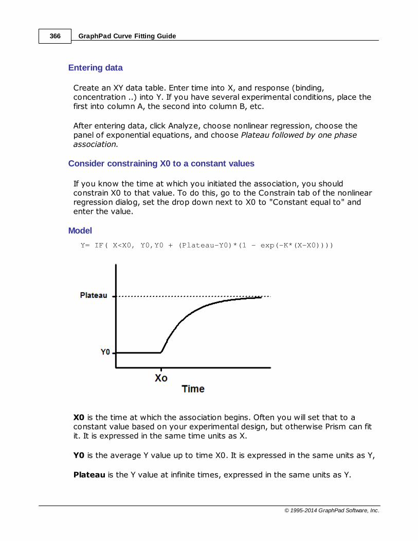
GraphPad Curve Fitting Guide366
© 1995-2014 GraphPad Software, Inc.
Entering data
Create an XY data table. Enter time into X, and response (binding,concentration ..) into Y. If you have several experimental conditions, place thefirst into column A, the second into column B, etc.
After entering data, click Analyze, choose nonlinear regression, choose thepanel of exponential equations, and choose Plateau followed by one phaseassociation.
Consider constraining X0 to a constant values
If you know the time at which you initiated the association, you shouldconstrain X0 to that value. To do this, go to the Constrain tab of the nonlinearregression dialog, set the drop down next to X0 to "Constant equal to" andenter the value.
Model
Y= IF( X<X0, Y0,Y0 + (Plateau-Y0)*(1 - exp(-K*(X-X0))))
X0 is the time at which the association begins. Often you will set that to aconstant value based on your experimental design, but otherwise Prism can fitit. It is expressed in the same time units as X.
Y0 is the average Y value up to time X0. It is expressed in the same units as Y,
Plateau is the Y value at infinite times, expressed in the same units as Y.

CURVE FITTING WITH PRISM 6 367
© 1995-2014 GraphPad Software, Inc.
K is the rate constant, expressed in reciprocal of the X axis time units. If X is inminutes, then K is expressed in inverse minutes.
Tau is the time constant, expressed in the same units as the X axis. It iscomputed as the reciprocal of K.
Half-life is in the time units of the X axis. It is computed as ln(2)/K.
Span is the difference between Y0 and Plateau, expressed in the same units asyour Y values.
2.7.12.9 Equation: Two phase association
Introduction
An exponential decay equation models many chemical and biological processes.It is used whenever the rate at which something happens is proportional to theamount which is left.
A two-phase model is used when the outcome you measure is the result of thesum of a fast and slow exponential decay.
Entering data
Create an XY data table. Enter time into X, and response (binding,concentration ..) into Y. If you have several experimental conditions, place thefirst into column A, the second into column B, etc.
After entering data, click Analyze, choose nonlinear regression, choose thepanel of exponential equations, and choose Two phase association.
Consider constraining Plateau to a constant value of zero
If you have subtracted off any background signal, then you know the curve hasto plateau at Y=0. In this case, you should constrain the parameter Plateau tobe a constant value equal to zero. To do this, go to the Constrain tab of thenonlinear regression dialog, set the drop down next to Plateau to "Constantequal to" and enter the value 0.0.
Model
SpanFast=(Plateau-Y0)*PercentFast*.01SpanSlow=(Plateau-Y0)*(100-PercentFast)*.01Y=Y0+ SpanFast*(1-exp(-KFast*X)) + SpanSlow*(1-exp(-KSlow*X))
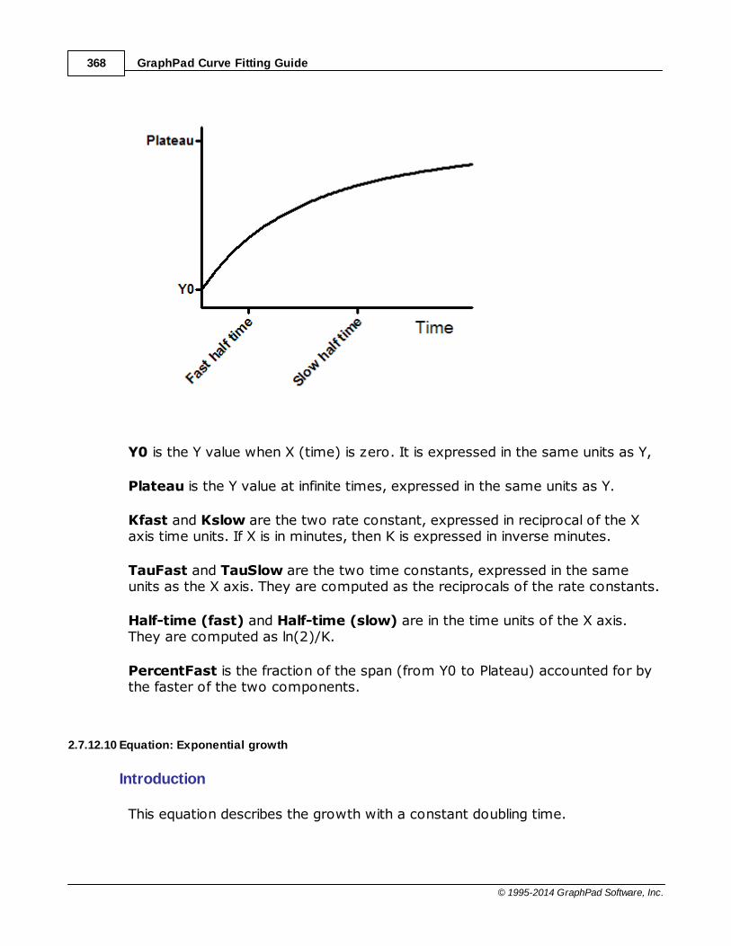
GraphPad Curve Fitting Guide368
© 1995-2014 GraphPad Software, Inc.
Y0 is the Y value when X (time) is zero. It is expressed in the same units as Y,
Plateau is the Y value at infinite times, expressed in the same units as Y.
Kfast and Kslow are the two rate constant, expressed in reciprocal of the Xaxis time units. If X is in minutes, then K is expressed in inverse minutes.
TauFast and TauSlow are the two time constants, expressed in the sameunits as the X axis. They are computed as the reciprocals of the rate constants.
Half-time (fast) and Half-time (slow) are in the time units of the X axis.They are computed as ln(2)/K.
PercentFast is the fraction of the span (from Y0 to Plateau) accounted for bythe faster of the two components.
2.7.12.10 Equation: Exponential growth
Introduction
This equation describes the growth with a constant doubling time.

CURVE FITTING WITH PRISM 6 369
© 1995-2014 GraphPad Software, Inc.
Entering data
Create an XY data table. Enter time into X, and response (cell number ..) into Y.If you have several experimental conditions, place the first into column A, thesecond into column B, etc.
After entering data, click Analyze, choose nonlinear regression, choose thepanel of exponential equations, and choose Exponential growth.
Consider constraining Y0 to a constant value
The parameter Y0 is the Y value at time zero. In many cases, you will know thisvalue precisely. If so, you should constrain that parameter to be a constantvalue. To do this, go to the Constrain tab of the nonlinear regression dialog, setthe drop down next to Y0 to "Constant equal to" and enter its value.
Model
Y=Y0*exp(k*X)
Y0 is the Y value when X (time) is zero. It is expressed in the same units as Y,
K is the rate constant, expressed in reciprocal of the X axis time units. If X is inminutes, then K is expressed in inverse minutes.
Tau is the time constant, expressed in the same units as the X axis. It iscomputed as the reciprocal of K.
Doubling-time is in the time units of the X axis. It is computed as ln(2)/K.

GraphPad Curve Fitting Guide370
© 1995-2014 GraphPad Software, Inc.
2.7.13 Lines
2.7.13.1 Key concepts: Fitting lines
Choosing nonlinear regression, rather than linear regression to fit a line
Prism offers separate analyses for linear regression and nonlinear regression.But the nonlinear regression analysis can fit a straight-line model. This is usefulwhen you want to take advantage of features in Prism's nonlinear regressionanalysis that Prism does not offer in its linear regression analysis, such as theability to compare two models , apply weighting , or automatically excludeoutliers . See a longer discussion of the advantages of using the nonlinearregression analysis to fit a straight line .
Fitting straight lines on graphs with nonlinear axes
The nonlinear regression analysis fits the data, not the graph. Since Prism letsyou choose logarithmic or probability axes, some graphs with data points thatform a straight line follow nonlinear relationships. Prism's collection of "Lines"equations includes those that let you fit nonlinear models to graphs that appearlinear when the X axis is logarithmic, the Y axis is logarithmic, both axes arelogarithmic, or when the Y axis uses a probability scale. In these cases, linearregression will fit a straight line to the data but the graph will appear curvedsince an axis (or both axes) are not linear. In contrast, nonlinear regression toan appropriate nonlinear model will create a curve that appears straight onthese axes.
Segmental linear regression
Segmental regression fits one line to all data points with X less than somevalue X0, and another line to all points with X greater than X0, ensuring that thetwo lines intersect at X0.
Segmental linear regression is helpful when X is time, and you did something attime=X0 to change the slope of the line. Perhaps you injected a drug, or rapidlychanged the temperature. In these cases, your model really does have twoslopes with a sharp transition point.
157 158
59
82
374

CURVE FITTING WITH PRISM 6 371
© 1995-2014 GraphPad Software, Inc.
2.7.13.2 Equation: Fitting a straight line with nonlinear regression
Introduction
Linear regression fits a straight line through your data. Nonlinear regression fitsany model, which includes a straight line model. Prism offers separate analysesfor linear regression and nonlinear regression, so you can choose either one tofit a line.
Prism's nonlinear regression analysis offers more options than its linearregression analysis , such as the ability to compare two models , applyweighting , automatically exclude outliers and perform normality testson the residuals. See a longer discussion of the advantages of using thenonlinear regression analysis to fit a straight line .
Step by step
Create an XY data table. There is one X column, and many Y columns. If youhave several experimental conditions, place the first into column A, the secondinto column B, etc.
After entering data, click Analyze, choose nonlinear regression, choose thepanel equations for lines, and choose Straight line.
Model
Y= YIntercept + Slope*X
Interpret the parameters
YIntercept is the Y value where the line intersects the Y axis.
Slope is the slope of the line, expressed in Y units divided by X units.
Special forms of the linear regression equation
Horizontal line
If you constrain the slope to be zero, the line will be horizontal. The onlyparameter is the Y intercept. Prism has this model built in as "horizontal line".The best-fit value of the Y intercept is the mean of all the Y values. The modelis:
Y = Mean + 0*X
13 157
158 59 185
82

GraphPad Curve Fitting Guide372
© 1995-2014 GraphPad Software, Inc.
Prism requires that all equations include X. Here X is multiplied by zero, so it ispresent (as required) but has no effect.
Line through origin
If you constrain the Y intercept to be zero, the line has to go through the origin(X=0, Y=0). Prism has this "Line through origin " model built in:
Y=Slope*X
The only parameter is the slope.
2.7.13.3 Equation: Line through origin
Introduction
Prism's linear regression analysis fits a straight line through your data, andlets you force the line to go through the origin. This is useful when you are surethat the line must begin at the origin (X=0 and Y=0).
Prism's nonlinear regression offers the equation Line through origin. It offersmore options than its linear regression analysis , such as the ability tocompare two models , apply weighting , automatically exclude outliersand perform normality tests on the residuals. See a longer discussion of theadvantages of using the nonlinear regression analysis to fit a straight line .
When to force the line through the origin
In many scientific situations, it just makes sense that when X=0, Y must alsoequal 0, so the line should be forced to go through the origin (X=0, Y=0). Buteven in these situations, it can make sense to fit an ordinary linear regressionline that also fits the intercept. The data you are analyzing may be far from theorigin, and you may get a better fit through the points (what you care about)when you don't force the line to go through the origin. This can happen whenthe true model is curved (beginning at the origin), so a line through the datapoints that is not forced to the origin may fit a whole lot better than line forcedto go through the origin.
Prism makes it easy to compare the fit that goes through the origin with onethat doesn't.
Step by step
Create an XY data table. There is one X column, and many Y columns. If youhave several experimental conditions, place the first into column A, the secondinto column B, etc.
372
76
13
157 158 59
185
82
157

CURVE FITTING WITH PRISM 6 373
© 1995-2014 GraphPad Software, Inc.
After entering data, click Analyze, choose nonlinear regression, choose thepanel equations for lines, and choose Line Through Origin
Model
Y= Slope*X
Slope is the slope of the line, expressed in Y units divided by X units. Itestimates the ratio of Y/X in the entire population.
Weighting
In situations where linear regression through the origin is appropriate, it iscommon for the variation among replicate Y values increases as X (and Y)increase. Prism provides two weighting choices (in the Weights tab) that areused in this situation. Weight by 1/X2 when you think the variance in Y isproportional to the square of X, which means the SD among Y values isproportional to X.Weight by 1/X if you think the variance in Y is proportional toX.
R2 when fitting a line through the origin
When you constrain a line to go through a point, there are two possible waysto compute R2:
Compare the fit of the best-fit line with the fit of a horizontal line at the mean
Y value. But that null hypothesis (horizontal line through the Ymean) doesn'tobey the constraint that it go through the origin.
Compare the best-fit line with a horizontal line at Y=0. This obeys the
constraint, but often fits the data really badly, pushing up the R2 value.
When you use nonlinear regression to fit a line through the origin, Prism usesthe first definition above. If you use linear regression, and ask Prism toconstrain the line to go through the origin, it simply will not report R2 at all.
Reference
1. J. G. Eisenhauer, Regression through the Origin. Teaching Statistics 25, 76–80(2003).

GraphPad Curve Fitting Guide374
© 1995-2014 GraphPad Software, Inc.
2.7.13.4 Equation: Segmental linear regression
Introduction
Segmental regression fits one line to all data points with X less than some valueX0, and another line to all points with X greater than X0, while ensuring that thetwo lines intersect at X0.
Segmental linear regression is helpful when X is time, and you did something attime=X0 to change the slope of the line. Perhaps you injected a drug, or rapidlychanged the temperature. In these cases, your model really does have twoslopes with a sharp transition point.
In other cases, the true model has the slope gradually changing. The data fit acurve, not two straight lines. In this situation, fitting the data with segmentallinear regression is not helpful.
Caution
Don't use segmental linear regression to analyze a biphasic Scatchard orLineweaver-Burk plot. A biphasic Scatchard plot follows a curve, not twointersecting lines. There is no abrupt break point. You should fit the original datato a two-site binding curve instead.
Step by step
Create an XY data table. Enter time into X, and your measurements into Y. Ifyou have several experimental conditions, place the first into column A, thesecond into column B, etc.
After entering data, click Analyze, choose nonlinear regression, choose thepanel equations for lines, and choose Segmental linear regression.
Model
Y1 = intercept1 + slope1*X YatX0 = slope1*X0 + intercept1Y2 = YatX0 + slope2*(X – X0) Y = IF(X<X0, Y1, Y2)
The first line of the equation defines the first line segment from its intercept andslope.
The second line of the equation computes the Y value of the first regression at

CURVE FITTING WITH PRISM 6 375
© 1995-2014 GraphPad Software, Inc.
the right end of that segment, when X=X0.
The third line of the equation computes the second regression segment. Sincewe want a continuous line, the Y value at the left end of the second segmentmust equal the Y value at the right end of the first segment (YatX0). The Yvalue at any other position along the second segment equals YatX0 plus theincrease due to the second regression line. That increase equals the slope of thesecond segment (slope2) times the distance from X0 to X.
The final line defines Y for all values of X. If X is less than X0 then Y is set equalto Y1. Otherwise Y is set equal to Y2.
Interpret the parameters
Intercept1 is the Y value where the first line segment intersects the Y axis.
Slope1 is the slope of the first line segment, expressed in Y units divided by Xunits.
Intercept2 is the Y value where the second (rightmost) line segmentintersects the Y axis.
Slope2 is the slope of the second line segment, expressed in Y units divided byX units.
X0 is the X value where the two line segments intersect. Often you will want toconstrain this to a constant value equal to the time you applied an experimentalintervention.

GraphPad Curve Fitting Guide376
© 1995-2014 GraphPad Software, Inc.
Extending to three segments
Prism does not include an equation for segmental regression with threesegments, but you could enter this equation as an user-defined equation:
Y1 = intercept1 + slope1*X
YatX0 = intercept1 + slope1*X0 Y2 = YatX0 + slope2*(X – X0)YatX1 = YatX0 + slope2*(X1-X0)Y3 = YatX1 + slope3*(X – X1)Y = IF(X<X0, Y1, IF(X<X1, Y2, Y3))
.
2.7.13.5 Equation: Fitting a straight line on a semi-log or log-log graph
Straight lines on graphs with logarithmic axes
The nonlinear regression analysis fits the data, not the graph. Since Prism letsyou choose logarithmic axes, some graphs with data points that form a straightline follow nonlinear relationships. Prism's collection of "Lines" equations includesthose that let you fit nonlinear models to graphs that appear linear when the Xaxis is logarithmic, the Y axis is logarithmic, or both axes are logarithmic. Inthese cases, linear regression will fit a straight line to the data but the graph willappear curved since an axis (or both axes) are not linear. In contrast, nonlinearregression to an appropriate nonlinear model will create a curve that appearsstraight on these axes.
Entering and fitting data
1.Create an XY table, and enter your X and Y values.
2.Go to the graph, double click on an axis to bring up the Format Axis dialog.Change one or both axes to a logarithmic scale.
3.Click Analyze, choose Nonlinear regression (not Linear regression) and thenchoose one of the semi-log or log-log equations from the "Lines" section ofequations.

CURVE FITTING WITH PRISM 6 377
© 1995-2014 GraphPad Software, Inc.
Equations
Semilog line -- X axis is logarithmic, Y axis is linear
Y=Yintercept + Slope*log(X)
On semilog axis On linear axes
Semilog line -- X axis is linear, Y axis is logarithmic
Y=10^(Slope*X + Yintercept)
On semilog axis On linear axes
Log-log line -- Both X and Y axes are logarithmic
Y = 10^(slope*log(X) + Yintercept)

GraphPad Curve Fitting Guide378
© 1995-2014 GraphPad Software, Inc.
On log-log axes On linear axes
Since both axes are transformed the same way, the graph is linear on both setsof axes. But when you fit the data, the two fits will not be quite identical.
Parameters
In all three equations, Y intercept is in units of the Y values, and Slope is in unitsof the Y values divided by units of the X values.
An alternative way to handle these data
The nonlinear regression analysis minimizes the sum of the squares of thedifference between the actual Y value and the Y value predicted by the curve.This is not the same as minimizing the sum of squares of the distances (asseen on the graph) between points and curve. In the graph below, the twovertical lines look the same distance but one represents a difference of 9 Yunits, and the other a difference of 900.

CURVE FITTING WITH PRISM 6 379
© 1995-2014 GraphPad Software, Inc.
An alternative approach, that might be better in some circumstances, is to usePrism's transform analysis to transform Y (and maybe also X) to logarithms.Then perform linear regression on the logarithms. The regression results will notbe the same as using nonlinear regression on log axes.
2.7.13.6 Equation: Fitting a straight line on a graph with a probability axis
Fitting straight lines on graphs with nonlinear axes
The nonlinear regression analysis fits the data, not the graph. If you chooseprobability Y axis, graphs with data points that form a straight line follownonlinear relationships. Prism's collection of "Lines" equations includes thosethat let you fit nonlinear models to graphs that appear linear when the Y axis isa probability axis. In these cases, linear regression will fit a straight line to thedata but the graph will appear curved since an axis (or both axes) are notlinear. In contrast, nonlinear regression to an appropriate nonlinear model willcreate a curve that appears straight on these axes.
Entering and fitting data
1.Create an XY table, and enter your X and Y values.
2.Go to the graph, double click on an axis to bring up the Format Axis dialog.Change the Y axis to a probability scale.
3.Click Analyze, choose Nonlinear regression (not Linear regression) and thenchoose one of the Cumulative Gaussian distribution equations from the"Lines" section of equations.
Equations
Cumulative Gaussian - Y values are percentages
Top=100z=(X-Mean)/SDY=Top * zdist(z)

GraphPad Curve Fitting Guide380
© 1995-2014 GraphPad Software, Inc.
On probability axis On linear axis
Cumulative Gaussian - Y values are fractions
Top=1z=(X-Mean)/SD
Y=Top * zdist(z)
On semilog axis On linear axes
Parameters
Mean is the average of the original distribution, from which the frequencydistribution was created.
SD is the standard deviation of the original distribution.
Both of these parameters are expressed in the same units as the X valuesplotted on the graph, which is the same as the Y values in the originaldistribution from which the frequency distribution was generated.

CURVE FITTING WITH PRISM 6 381
© 1995-2014 GraphPad Software, Inc.
2.7.14 Polynomial
2.7.14.1 Key concepts: Polynomial
Usefulness of polynomial models
There are two situations where you might want to choose a polynomial model:
Your scientific model is described by a polynomial equation. This is rare in
biology. Few chemical or pharmacological models are described bypolynomial equations.
You don't have a scientific model, but want to fit a curve to interpolate
unknown values. With this goal, you often don't care much about the detailsof the model. Instead, you care only about finding a model that goes nearthe data points. Polynomial models often work well.
Which polynomial model?
The order of a polynomial model expresses how many terms it has. Prismoffers up to a sixth order equation (and it would be easier to enter higher orderequations). The higher order equations have more inflection points.
Choosing the best polynomial model is often a matter of trial and error. If thecurve doesn't follow the trend of your data, pick a higher order equation. If itwiggles too much, pick a lower order equation.
How are polynomial models special?
To a mathematician, polynomial models are very special. Strictly speaking, polynomialmodels are not 'nonlinear'. Even though a graph of X vs. Y is curved (in all but somespecial cases), the derivative of Y with respect to the parameters is linear.
Because polynomial models are not nonlinear, it is possible (but not with Prism) to fitpolynomial models without fussing with initial values. And the fit can be in one step,rather than the iterative approach used for nonlinear models.
Since Prism treats polynomial models the same way it treats nonlinear models, it doesrequire initial values (it chooses 1.0 for each parameter automatically). It doesn't matterwhat values are used -- polynomial regression cannot encounter false minima . 206

GraphPad Curve Fitting Guide382
© 1995-2014 GraphPad Software, Inc.
Why you should choose a centered polynomial equation
There are two problems with polynomial fits, often solved by centering:
When the X values are large, and start well above zero (for example, when X is a calendaryear), taking the very large X values to large powers can lead to math errors.
Even when the X values are not large, the parameters of the model are intertwined, so havehigh covariance and dependency. This results in large standard errors, wide confidenceintervals, and huge confidence or prediction bands.
Both these problems are solved by using a centered polynomial model. The ideaof centering is simple. Subtract the mean of all X values from each X value, anduse those differences instead of X in the model.
Fitting the centered model leads to exactly the same curve (unless the regular approach led to math errors). Accordingly, the sum-of-squares are R2 are thesame, as are results of model comparisons.However, the parameters havedifferent meanings, so have different best-fit values (except the first parameterwhich is the same), different standard errors and confidence intervals, smallercovariances and dependencies, and tighter confidence/prediction bands.
Read more about centered polynomial models.
2.7.14.2 Centered polynomial equations
Included in Prism, are both a set of ordinary polynomial equations and also aset of centered polynomial equations. For example, when you look in the list ofpolynomials you'll see both 'Second order polynomial' and 'Centered secondorder polynomial'. We recommend always choosing one of the centeredequations instead of an ordinary polynomial equation. This page explains why.
What's wrong with ordinary polynomial models?
The standard polynomial models look like this:
Y= B0 + B1*X +B2*X^2
More terms are included with the higher order equations.
There are two problems with polynomial fits:
When the X values are large, and start well above zero (for example, when X
is a calendar year), taking the very large X values to large powers can lead tomath overflow. Even if the program doesn't report any math error, theresults can be inaccurate. Some coefficients will be positive and somenegative, so the value of Y depends on subtracting huge numbers from other
382

CURVE FITTING WITH PRISM 6 383
© 1995-2014 GraphPad Software, Inc.
huge numbers, leading to imprecise results.
Even when the X values are not large, the parameters of the model are
intertwined, so have high covariance and dependency. This results in largestandard errors, wide confidence intervals, and very wide confidence orprediction bands. In many cases, this problem is severe enough that Prismreports that the results are 'ambiguous' and so doesn't report confidenceintervals for all the parameters and can't graph confidence bands.
What are centered polynomial models?
Both problems go away when the X values are centered. The idea of centeringis to subtract the mean X from all X values before fitting the model. This can bedone as part of nonlinear regression, using this model:
XC = X - XmeanY= B0 + B1*XC +B2*XC^2
Here XC is the centered X value, equal to the X value minus Xmean, which isthe mean of all X values. In other words, XC is the distance of any X value fromthe mean of all X values. Xmean is constant, and not a parameter that Prismtries to fit. Of course, you can include more terms in the definition of Y tocreate higher order polynomial equations.
The advantages of centered models
Fitting the centered model leads to exactly the same curve (unless the regular approach led to math errors). Accordingly, the sum-of-squares is the same, asare results of model comparisons.
However, the centered equation has reparameterized the model. Theparameters have different meanings, so have different best-fit values (exceptthe first parameter which is the same), different standard errors and confidenceintervals, smaller covariances and dependencies, and tighter confidence/prediction bands.
How centered models are implemented in Prism
You can fit data to a built-in centered polynomial equation without knowing howPrism implements the model. If you are curious, read on.
The built-in set of centered polynomial equations, written as shown above,constrain the parameter XMean to equal the mean of X value by constraining itto equal a "Data set constant (= Mean X)".
If you open a file using centered polynomial regression in an version of Prism

GraphPad Curve Fitting Guide384
© 1995-2014 GraphPad Software, Inc.
prior to 5.02 or 5.0b, that constraint will be lost, and centered polynomialregression won't work.
2.7.14.3 Equations: Polynomial models
Step by step
Create an XY data table. There is one X column, and many Y columns. If youhave several experimental conditions, place the first into column A, the secondinto column B, etc.
After entering data, click Analyze, choose nonlinear regression, choose thepanel equations for polynomial equations, and choose one.
The "order" of a polynomial equation tells you how many terms are in theequation. Prism offers first to sixth order polynomial equations (and you couldenter higher order equations as user-defined equations if you need them).Higher order models wiggle more than do lower order models. Since theequation rarely corresponds to a scientific model, use trial and error. If it isn'tclose enough to the data, pick a higher order equation. If it wiggles too much,pick a lower order equation.
Polynomial models
Order Equation
First Y=B0 + B1*X (straight line)
Second Y=B0 + B1*X + B2*X^2 (quadratic equation)
Third Y=B0 + B1*X + B2*X^2 + B3*X^3
Fourth Y=B0 + B1*X + B2*X^2 + B3*X^3 + B4*X^4
Fifth Y=B0 + B1*X + B2*X^2 + B3*X^3 + B4*X^4 + B5*X^5
Sixth Y=B0 + B1*X + B2*X^2 + B3*X^3 + B4*X^4 + B5*X^5 +B6*X^6
There is no general way to interpret the coefficients B0, B1, etc. In most cases,the goal of fitting a polynomial model is to make a curve that looks good, andthe parameters really don't matter.

CURVE FITTING WITH PRISM 6 385
© 1995-2014 GraphPad Software, Inc.
Centered polynomial models
The Centered polynomial models are identical to the ones listed above, withone exception. Wherever X appears above, replace it with (X - XMean), whereXMean is the mean of all X values (for rows that have Y values). Using acentered model can avoid computer math problems (overflows), and werecommend that you use them routinely.
2.7.15 Gaussian
2.7.15.1 Key concepts: Gaussian
What is a frequency distribution?
All the equations in this section fit frequency distributions. The X valuesrepresent Y values in the original data set, and the Y values are the frequency orcumulative frequency.
Prism can create a frequency distribution from column data, using an analysiscreated for that purpose (called, of course, Frequency Distribution).
What is a cumulative frequency distribution?
A frequency distribution plots the number of observations as a function ofvalue. A cumulative frequency distribution plots the cumulative number ofobservations as a function of value. Each Y value is the number of observationsin the original data set that have a value less than or equal to the X value.
The Y values can be expressed as the counted number of observations, asfractions or as percentages.
382
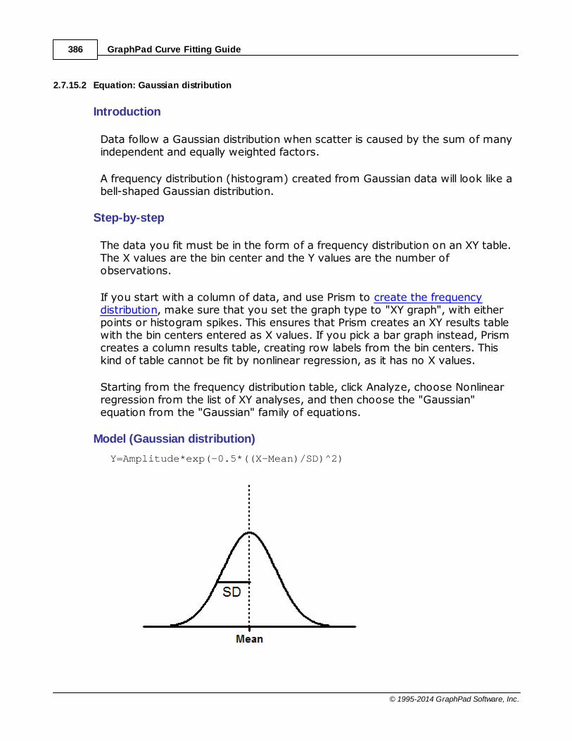
GraphPad Curve Fitting Guide386
© 1995-2014 GraphPad Software, Inc.
2.7.15.2 Equation: Gaussian distribution
Introduction
Data follow a Gaussian distribution when scatter is caused by the sum of manyindependent and equally weighted factors.
A frequency distribution (histogram) created from Gaussian data will look like abell-shaped Gaussian distribution.
Step-by-step
The data you fit must be in the form of a frequency distribution on an XY table.The X values are the bin center and the Y values are the number ofobservations.
If you start with a column of data, and use Prism to create the frequencydistribution, make sure that you set the graph type to "XY graph", with eitherpoints or histogram spikes. This ensures that Prism creates an XY results tablewith the bin centers entered as X values. If you pick a bar graph instead, Prismcreates a column results table, creating row labels from the bin centers. Thiskind of table cannot be fit by nonlinear regression, as it has no X values.
Starting from the frequency distribution table, click Analyze, choose Nonlinearregression from the list of XY analyses, and then choose the "Gaussian"equation from the "Gaussian" family of equations.
Model (Gaussian distribution)
Y=Amplitude*exp(-0.5*((X-Mean)/SD)^2)

CURVE FITTING WITH PRISM 6 387
© 1995-2014 GraphPad Software, Inc.
Amplitude is the height of the center of the distribution in Y units.
Mean is the X value at the center of the distribution.
SD is a measure of the width of the distribution, in the same units as X.
The mean and SD will not be identical to the mean and SD computed directlyfrom the raw data. There are two reasons for the discrepancy. The first is thatcreating the frequency distribution requires a fairly arbitrary decision about binwidth, and that will influence the best-fit values of Mean and SD. The secondreason is that the nonlinear regression assumes that the residuals (thedistances of the points from the curve) follow a Gaussian distribution. Thisassumption won't be exactly true in a frequency distribution.
Model (sum of two Gaussian distributions)
If your data are a mixture of values sampled from two Gaussian distributions,fit the frequency distribution to a model of the sum of two Gaussiandistributions.
One=Amplitude1*exp(-0.5*((X-Mean1)/SD1)^2)Two=Amplitude2*exp(-0.5*((X-Mean2)/SD2)^2)Y= One + Two
Amplitude1 and Amplitude2 are the heights of the center of the distributionin Y units.
Mean1 and Mean2 are the X values at the center of the two distributions.
SD1 and SD2 are measures of the widths of the distributions, in the same unitsas X.
Prism is not very smart about assigning initial values to the parameters. If youhave trouble getting this model to fit, try fussing with the initial parametervalues.
Area under a Gaussian distribution
The area under a Gaussian distribution equals Amplitude*SD/0.3989. Thatconstant equals the reciprocal of the square root of two pi.

GraphPad Curve Fitting Guide388
© 1995-2014 GraphPad Software, Inc.
2.7.15.3 Equation: Log Gaussian distribution
Introduction
Data follow a Gaussian distribution when scatter is caused by the sum of manyindependent and equally weighted factors.
When scatter is caused by the product of many independent and equallyweighted factors, data follow a log Gaussian distribution. When plotted on alinear X axis, this is skewed to the right (see below). When plotted on alogarithmic X axis, it looks like a bell-shaped Gaussian distribution.
Step-by-step
The data must be in the form of a frequency distribution on an XY table. The Xvalues are the bin center and the Y values are the number of observations.
If you start with a column of data, and use Prism to create the frequencydistribution, make sure that you set the graph type to "XY graph", with eitherpoints or histogram spikes. This ensures that Prism creates an XY results tablewith the bin centers entered as X values. If you pick a bar graph instead, Prismcreates a column results table, creating row labels from the bin centers. Thiskind of table cannot be fit by nonlinear regression, as it has no X values.
Starting from the frequency distribution table, click Analyze, choose Nonlinearregression from the list of XY analyses, and then choose the "logGaussian"equation from the "Gaussian" family of equations.
Model
Y=Amplitude*exp(-0.5*(ln(X/Center)/Width)^2)

CURVE FITTING WITH PRISM 6 389
© 1995-2014 GraphPad Software, Inc.
Amplitude is the height of the center of the distribution in Y units.
Center is the X value at the peak of the distribution.
Width is a measure of the width of the distribution. It is also called thegeometric standard deviation. If you transformed all the X values to theirnatural logarithms, and then fit a Gaussian distribution, the SD would equal theWidth from this log Gaussian fit.
A more standard form of the model
A more standard form of the model (from Wikipedia or MathWorld) is:
Y= (1/(X*S*sqrt(2*pi)))*exp(-0.5*(ln(X)-M)^2/(S^2))
This standard form of the equation doesn't have a parameter describing theamplitude as that is computed from S (what we call Width) and M (what we callCenter). The area under the curve, using the equation above, is 1.0. To allowfor a variable area under the curve (and thus a variable maximum height),you'd need to multiply that equation by an Area parameter.
2.7.15.4 Equation: Cumulative Gaussian distribution
Introduction
A frequency distribution plots the number of observations as a function ofvalue. A cumulative frequency distribution plots the cumulative number ofobservations as a function of value. Each Y value is the number of observationsin the original data set that have a value less than or equal to the X value.
The advantage of creating a cumulative distribution is that you don't have tomake any choice regarding bin width.
If your data follow a Gaussian distribution, the cumulative distribution has asigmoidal shape.

GraphPad Curve Fitting Guide390
© 1995-2014 GraphPad Software, Inc.
Step-by-step
1.Create an XY table, and enter your X and Y values. The X values correspondto the value in the original data set, and the Y values are the number (orfraction or percent) of values in the original data set that are less than orequal to the Y value.
Alternatively, enter a stack of values onto a Column data table, and runthe frequency distribution analysis choosing to create a cumulativefrequency distribution with no bins.
2.From the cumulative frequency distribution, click Analyze, choose Nonlinearregression and then choose one of the Cumulative Gaussian distributionequations from the "Gaussian" group of equations.
3.If your data are entered as counts (rather than percentages or fractions)constrain N to a constant value equal to the number of observations.
Models
The details of the model depend on whether the Y values are percentages,fractions or counts.
Here is the model if the data are percentages, so the last Y value equals 100.
Top=100z=(X-Mean)/SDY=Top * zdist(z)
Here is the model if the data are fractions, so the first line of the model definesTop to equal 1.00.
Top=1.0z=(X-Mean)/SDY=Top * zdist(z)

CURVE FITTING WITH PRISM 6 391
© 1995-2014 GraphPad Software, Inc.
And finally, here is the model if the data are numbers of observations, so thelargest value equals the number of observations (N). In this case, you shouldconstrain N to be a constant value equal to the number of observations.
z=(X-Mean)/SDY=N * zdist(z)
Mean is the average of the original distribution, from which the frequencydistribution was created.
SD is the standard deviation of the original distribution.
Both of these parameters are expressed in the same units as the X valuesplotted on the graph, which is the same as the Y values in the originaldistribution from which the frequency distribution was generated.
Plotting on a log Y axis
If you choose a Y axis with a probability scale, then the cumulative Gaussiandistribution appears as a straight line. For this reason, the cumulative Gaussianmodels are part of both "Lines" families of equations as well as the "Gaussian"family. The two listings are identical.
2.7.15.5 Equation: Lorentzian
Introduction
A Lorentzian distribution is bell shaped, but has much wider tails than does aGaussian distribution.

GraphPad Curve Fitting Guide392
© 1995-2014 GraphPad Software, Inc.
Step-by-step
The data must be in the form of a frequency distribution on an XY table. The Xvalues are the bin center and the Y values are the number of observations.
If you start with a column of data, and use Prism to create the frequencydistribution, make sure that you set the graph type to "XY graph", with eitherpoints or histogram spikes. This ensures that Prism creates an XY results tablewith the bin centers are entered as X values. If you pick a bar graph instead,Prism creates a column results table, creating row labels from the bin centers.This kind of table cannot be fit by nonlinear regression, as it has no X values.
Starting from the frequency distribution table, click Analyze, choose Nonlinearregression from the list of XY analyses, and then choose the "Lorentzian"equation from the "Gaussian" family of equations.
Model (Lorentzian distribution)
Y=Amplitude/(1+((X-Center)/Width)^2)
Amplitude is the height of the center of the distribution in Y units.
Center is the X value at the center of the distribution.
Width is a measure of the width of the distribution, in the same units as X. Thisis not identical to a standard deviation, but has the same general meaning.
Model (sum of two Lorentzian distributions)
One=Amplitude1/(1+((X-Center1)/Width1)^2)Two=Amplitude2/(1+((X-Center2)/Width2)^2)Y=One + Two
Amplitude1 and Amplitude2 are the heights of the center of the distributionin Y units.
Center1 and Center2 are the X values at the center of the two distributions.
Width1 and Width2 are measures of the widths of the distributions, in thesame units as X.
Prism is not very smart about assigning initial values to the parameters. If youhave trouble getting this model to fit, try fussing with the initial parametervalues.

CURVE FITTING WITH PRISM 6 393
© 1995-2014 GraphPad Software, Inc.
2.7.16 Sine waves
2.7.16.1 Standard sine wave
Introduction
Sine waves describe many oscillating phenomena.
Step by step
Create an XY data table. There is one X column, and many Y columns. If youhave several experimental conditions, place the first into column A, the secondinto column B, etc.
After entering data, click Analyze, choose nonlinear regression, choose thepanel of equations for sine waves, and choose Standard sine wave.
If you know the Y value is zero at time zero, then constrain PhaseShift to aconstant value of zero.
Model
Y= Amplitude*sin((2*pi*X/Wavelength)+PhaseShift)
Interpret the parameters
Amplitude is the height of top of the waves, in Y units.
Wavelength is the time it takes for a complete cycle, in units of X
Frequency is the number of cycles per time unit. It is calculated as thereciprocal of wavelength, and is expressed in the inverse of the time units of X.

GraphPad Curve Fitting Guide394
© 1995-2014 GraphPad Software, Inc.
PhaseShift is the earliest time when Y=0, in time units of X axis.
2.7.16.2 Damped sine wave
Introduction
Sine waves describe many oscillating phenomena. Often the peak of eachwave decreases or dampens as time goes on.
Step by step
Create an XY data table. There is one X column, and many Y columns. If youhave several experimental conditions, place the first into column A, the secondinto column B, etc.
After entering data, click Analyze, choose nonlinear regression, choose thepanel of equations for sine waves, and choose Damped sine wave.
If you know the Y value is zero at time zero, then constrain PhaseShift to aconstant value of zero.
Model
Y= Amplitude*exp(-K*X)*sin((2*pi*X/Wavelength)+PhaseShift
Interpret the parameters
Amplitude is the height of top of the waves, in Y units.
Wavelength is the time it takes for a complete cycle, in units of X
Frequency is the number of cycles per time unit. It is calculated as thereciprocal of wavelength, and is expressed in the inverse of the time units of X.
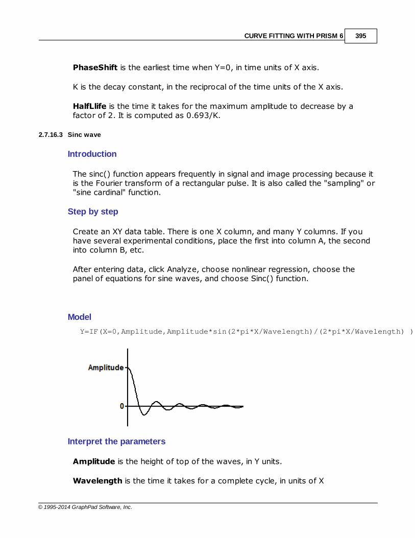
CURVE FITTING WITH PRISM 6 395
© 1995-2014 GraphPad Software, Inc.
PhaseShift is the earliest time when Y=0, in time units of X axis.
K is the decay constant, in the reciprocal of the time units of the X axis.
HalfLlife is the time it takes for the maximum amplitude to decrease by afactor of 2. It is computed as 0.693/K.
2.7.16.3 Sinc wave
Introduction
The sinc() function appears frequently in signal and image processing because itis the Fourier transform of a rectangular pulse. It is also called the "sampling" or"sine cardinal" function.
Step by step
Create an XY data table. There is one X column, and many Y columns. If youhave several experimental conditions, place the first into column A, the secondinto column B, etc.
After entering data, click Analyze, choose nonlinear regression, choose thepanel of equations for sine waves, and choose Sinc() function.
Model
Y=IF(X=0,Amplitude,Amplitude*sin(2*pi*X/Wavelength)/(2*pi*X/Wavelength) )
Interpret the parameters
Amplitude is the height of top of the waves, in Y units.
Wavelength is the time it takes for a complete cycle, in units of X

GraphPad Curve Fitting Guide396
© 1995-2014 GraphPad Software, Inc.
Frequency is the number of cycles per time unit. It is calculated as thereciprocal of wavelength, and is expressed in the inverse of the time units of X.
2.7.17 Classic equations from prior versions of Prism
2.7.17.1 Equation: One site binding (hyperbola)
This curve is known as a rectangular hyperbola, binding isotherm, or saturationbinding curve. Y is zero initially, and increases to a maximum plateau valueB
max.
This equation describes the equilibrium binding of a ligand to a receptor as afunction of increasing ligand concentration.
X is the concentration of the ligand.
Y is the specific binding.
Bmax is the maximum number of binding sites, expressed in the same units
as the Y-axis (usually radioactive counts per minute, sites per cell, or fmolof receptor per mg of tissue).
Kd is the equilibrium dissociation constant, expressed in the same units as
the X-axis (concentration). When the drug concentration equals Kd, half thebinding sites are occupied at equilibrium.

CURVE FITTING WITH PRISM 6 397
© 1995-2014 GraphPad Software, Inc.
This equation also describes the activity of an enzyme as a function ofsubstrate concentration. In this case, the variable labeled Bmax is really Vmax,the maximum enzyme activity, and the variable labeled Kd is really Km, theMichaelis-Menten constant.
2.7.17.2 Equation:Two site binding
This equation is an extension of the one site binding curve . It shows thebinding of a ligand to two receptors with different affinities (different Kd values).It also describes the enzyme activity as a function of substrate concentrationwhen two isozymes are present. The curve in the example has Kd values thatdiffer by a factor of ten, with equal Bmax values. Even with such a largedifference between Kd values, the curve is not obviously biphasic.
2.7.17.3 Equation: Sigmoidal dose-response
396

GraphPad Curve Fitting Guide398
© 1995-2014 GraphPad Software, Inc.
This is a general equation for a dose-response curve. It shows response as afunction of the logarithm of concentration. X is the logarithm of agonistconcentration and Y is the response. This equation is also called a three-parameter logistic equation.
The variable Bottom is the Y value at the bottom plateau; Top is the Y value atthe top plateau, and LogEC50 is the X value when the response is halfwaybetween Bottom and Top. LogEC50 is the logarithm of the EC50 (effectiveconcentration, 50%). With different kinds of variables, this variable issometimes called ED50 (effective dose, 50%), or IC50 (inhibitoryconcentration, 50%, used when the curve goes downhill).
This equation assumes a standard slope, where the response goes from 10%to 90% of maximal as X increases over about two log units. The next equation
allows for a variable slope.
2.7.17.4 Equation: Sigmoidal dose-response (variable slope)
398

CURVE FITTING WITH PRISM 6 399
© 1995-2014 GraphPad Software, Inc.
This equation extends the previous equation, but allows for a variable slope.This equation is also called a four-parameter logistic equation.
Bottom is the Y value at the bottom plateau.
Top is the Y value at the top plateau.
LogEC50 is the X value when the response is halfway between Bottom and
Top. With different kinds of variables, this variable is sometimes called ED50(effective dose, 50%), or IC50 (inhibitory concentration, 50%, used whenthe curve goes downhill).
HillSlope describes the steepness of the curve. This variable is called the Hill
slope, the slope factor, or the Hill coefficient. If it is positive, the curveincreases as X increases. If it is negative, the curve decreases as Xincreases. A standard sigmoid dose-response curve (previous equation) hasa Hill Slope of 1.0. When HillSlope is less than 1.0, the curve is moreshallow. When HillSlope is greater than 1.0, the curve is steeper. The Hillslope has no units.
2.7.17.5 Equation: One site competition
This equation describes the competition of a ligand for receptor binding. It isidentical to the sigmoid dose-response curve with HILLSLOPE = -1.0.
The variable LogEC50 is the concentration of the competitor required tocompete for half the specific binding. We use the term EC50 to be consistentwith the equations for the other sigmoid curves. The term IC50 is used morefrequently ("E" stands for effective; "I" stands for inhibitory).
Usually the Y values are total binding. If you enter specific binding instead, fixBOTTOM to have a constant value of zero. If you enter percent specific binding,also set TOP to be a constant equal to 100.

GraphPad Curve Fitting Guide400
© 1995-2014 GraphPad Software, Inc.
2.7.17.6 Equation: Two site competition
This equation describes the competition of a ligand for two types of receptors.The radioligand has identical affinities for both receptors, but the competitor hasa different affinity for each.
Y is binding (total or specific) and X is the logarithm of the concentration of theunlabeled ligand. FRACTION_1 is the fraction of the receptors that have anaffinity described by LogEC50_1. The remainder of the receptors have anaffinity described by LogEC50_2. If LogEC50_1 is smaller than LogEC50_2,then Fraction_1 is the fraction of high affinity sites. If LogEC50_1 is larger thanLogEC50_2, then Fraction_1 is the fraction of low affinity sites.
2.7.17.7 Equation: Boltzmann sigmoid

CURVE FITTING WITH PRISM 6 401
© 1995-2014 GraphPad Software, Inc.
This equation describes voltage dependent activation of ion channels. Itdescribes conductance (Y) as a function of the membrane potential (X).Conductance varies from BOTTOM to TOP. V50 is the potential at whichconductance is halfway between BOTTOM and TOP. SLOPE describes thesteepness of the curve, with a larger value denoting a shallow curve. Slope isexpressed in units of potential, usually mV, and is positive for channels thatactivate upon depolarization.
Under appropriate experimental conditions, you can use SLOPE to calculate thevalence (charge) of the ion moving across the channel. SLOPE equals RT/zFwhere R is the universal gas constant, T is temperature in °K, F is the Faradayconstant, and z is the valence. Since RT/F » -26 mV at 25°C, z = -26/SLOPE.
BOTTOM is commonly made a constant equal to 0.0. If you also make TOP aconstant equal to 1.0, then Y can be viewed as the fraction of channels that areactivated.
2.7.17.8 Equation: One phase exponential decay
This equation describes the kinetics such as the decay of radioactive isotopes,the elimination of drugs, and the dissociation of a ligand from a receptor.

GraphPad Curve Fitting Guide402
© 1995-2014 GraphPad Software, Inc.
X is time.
Y may be concentration, binding, or response. Y starts out equal to SPAN+PLATEAU and decreases to PLATEAU with a rate constant K.
The half-life of the decay is 0.6932/K.
SPAN and PLATEAU are expressed in the same units as the Y axis. K isexpressed in the inverse of the units used by the X axis. In manycircumstances, the plateau equals zero. When fitting data to this equation,consider fixing the plateau to a constant value of zero.
2.7.17.9 Equation: Two phase exponential decay
This equation describes a two phase exponential decay. Y starts out equal toSpan1+Span2+PLATEAU and decays to PLATEAU with fast and slowcomponents. The two half-lives are 0.6932/K1 and 0.6932/K2. In the figure,the two rate constants differ tenfold, but the spans were equal. The curve is notobviously biphasic, and it takes a very practiced eye to see that the curve doesnot follow a single phase model.
2.7.17.10 Equation: One phase exponential association

CURVE FITTING WITH PRISM 6 403
© 1995-2014 GraphPad Software, Inc.
This equation describes the pseudo-first order association kinetics of theinteraction between a ligand and its receptor, or a substrate and an enzyme. Yis either binding or enzyme activity. X is time.
Y starts out equal to zero and increases to a maximum plateau (at equilibrium)equal to YMAX. When X equals 0.6932/K, Y equals 0.5*YMAX.
2.7.17.11 Equation: Two phase exponential association
This is an extension of the exponential association to two phases,corresponding to a radioligand binding to two independent sites.
2.7.17.12 Equation: Exponential growth
This describes an exponential growth curve. Y is population size (perhaps cellnumber) and X is time. At X=0, Y equals START. Y increases geometrically witha doubling time equal to 0.6932/K.

GraphPad Curve Fitting Guide404
© 1995-2014 GraphPad Software, Inc.
Note: It is difficult to fit data to this equation with nonlinear regression, becausea tiny change in the initial values will drastically alter the sum-of-squares. Youmay need to override the initial values provided by Prism.
2.7.17.13 Equation: Power series
This versatile equation has many uses.
Fitting data to a power series model can be difficult. The initial values generatedautomatically by Prism are not very helpful (all four parameters are set to 1.0).you will probably need to enter better initial values in order to fit this equationto data. The initial values of B and D are important, because small changes inthose values can make a huge change in Y.
The equation is not defined, and leads to a floating point error, if X equals zeroand B or D are negative numbers or if X is negative and B or D are between 0.0and 1.0.
2.7.17.14 Equation: Sine wave
X is in radians. In most cases, you will want to fix BASELINE to a constant valueof zero. AMPLITUDE is the maximum height of the curve away from thebaseline. FREQUENCY is the number of complete oscillations per 1 X unit.
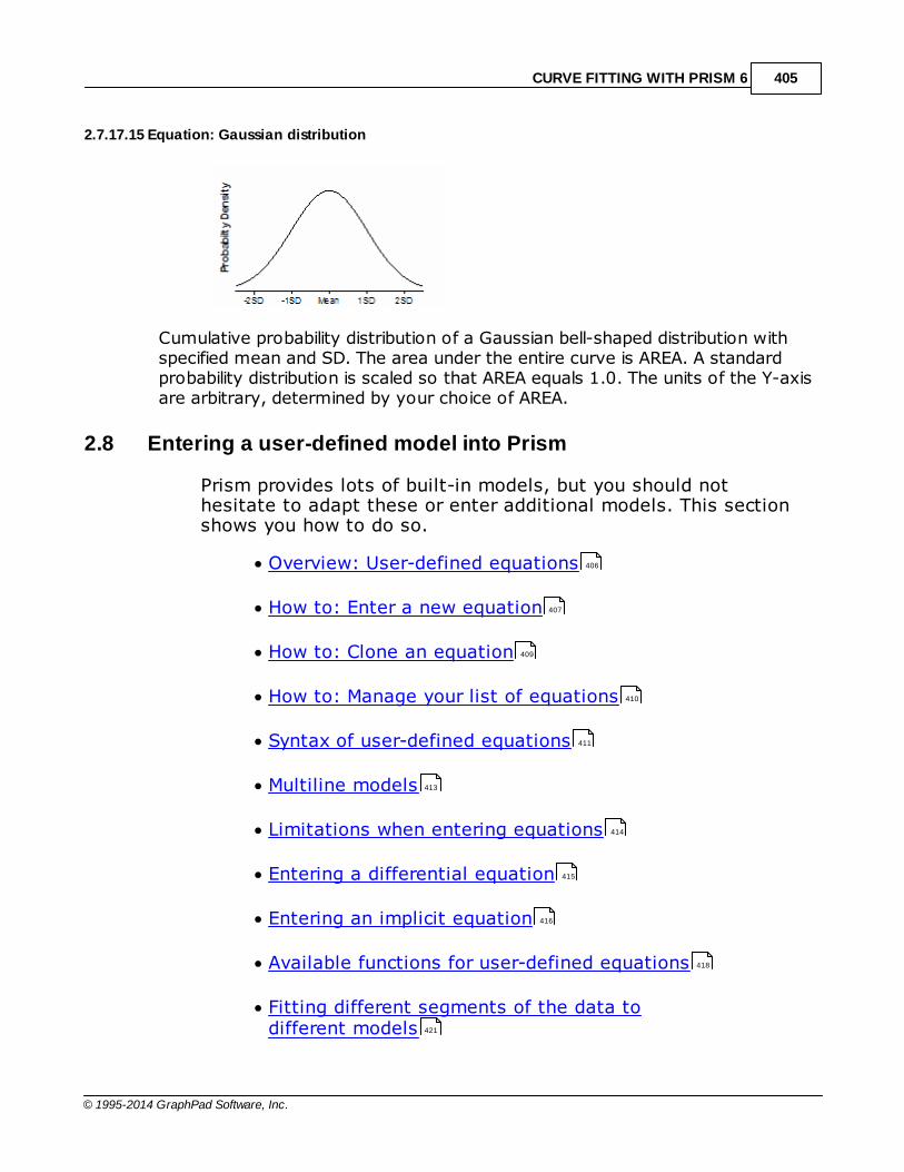
CURVE FITTING WITH PRISM 6 405
© 1995-2014 GraphPad Software, Inc.
2.7.17.15 Equation: Gaussian distribution
Cumulative probability distribution of a Gaussian bell-shaped distribution withspecified mean and SD. The area under the entire curve is AREA. A standardprobability distribution is scaled so that AREA equals 1.0. The units of the Y-axisare arbitrary, determined by your choice of AREA.
2.8 Entering a user-defined model into Prism
Prism provides lots of built-in models, but you should nothesitate to adapt these or enter additional models. This sectionshows you how to do so.
Overview: User-defined equations
How to: Enter a new equation
How to: Clone an equation
How to: Manage your list of equations
Syntax of user-defined equations
Multiline models
Limitations when entering equations
Entering a differential equation
Entering an implicit equation
Available functions for user-defined equations
Fitting different segments of the data todifferent models
406
407
409
410
411
413
414
415
416
418
421

GraphPad Curve Fitting Guide406
© 1995-2014 GraphPad Software, Inc.
Fitting different models to different data sets
Column constants
Defining equation with two (or more)independent variables
Rules for initial values
Default constraints
Transforms to report
2.8.1 Overview: User-defined equations
Few people will need to enter user-defined equations into Prism. If you need to do this, keepthese points in mind:
Rather than starting with a blank screen, it is usually much easier to clone an existingequation , and then modify it.
The syntax Prism uses is pretty standard. But use plenty of parentheses, so there is nodoubt about what the equation means. Many people have made the mistake of entering "A/B+C" expecting Prism to divide A by the sum of B plus C. Instead, Prism first dives A by B,and then adds that quotient to C. Writing the equation with parentheses as "A/(B+C)" avoidsany ambiguity.
Prism lets you use many standard mathematical functions when defining your model.Most of these are standard. But watch out for a few that are implemented differently indifferent languages. The log() function in Prism is common (base 10) log. If you want to usenatural logs, use the ln() function. The sqr() function in Prism squares the value, while thesqrt() function computes the square root.
Prism lets you write an equation in such a way that different models are fit to different datasets .
When you write a model using several lines , Prism evaluates from the top down. Thisfollows the conventions of all computer languages, but is opposite to how mathematical textbooks present complicated equations.
After writing the equation, don't forget to define rules for initial values . If you don't do this,you'll need to enter initial estimated values for each parameter every time you fit the modelto data.
When you enter a new equation, Prism also lets you define default constraints andtransforms to report . These features are optional, so you can skip them when firstlearning about user-defined equations.
423
424
426
433
437
438
409
418
423
413
433
437
438

CURVE FITTING WITH PRISM 6 407
© 1995-2014 GraphPad Software, Inc.
2.8.2 How to: Enter a new equation
Entering an equation
Prism comes with many built-in equations, but you will often want to enter adifferent equation. To do so, click the New button on the top of the Fit tab ofthe Nonlinear regression dialog.
A drop down menu lets you choose to enter a new equation, clone an existingone, or import an equation from a saved .PZF file.

GraphPad Curve Fitting Guide408
© 1995-2014 GraphPad Software, Inc.
Name, definition, tip and description
Equation type
Choose whether you are entering an ordinary explicit equation (that defines Yas a function of X and parameters), an implicit equation (Y appears on bothsides of the equals sign) or a differential equation (which defines the derivativeof Y with respect to X).
Name
Enter a name you will recognize, so you can choose the equation again. Thename also appears on the results table, so make it both descriptive andconcise.
Definition
Write the math that defines Y as a function of X and one or more parameters.Read the details of equation syntax , a list of available math functions youcan use, and how to fit different models to different ranges of X values andto different data sets .
Tip
The tip appears below the equation list in the Fit tab of the Nonlinear regressiondialog. Use it to distinguish among similar equations. Tips are optional, and mustbe short (a few sentences).
Description
The description can be up to several paragraphs. Anyone choosing the equationcan view the description (and the math) by clicking the Edit or View button. Thisis a good place to document the source of the equation, its assumptions, unitsof the parameters, etc.
Rules for initial values
Nonlinear regression must begin with initial estimated values for eachparameter. You can enter values directly, or enter a rule whereby Prism cancompute the initial value from the range of the X and Y values. Learn more .
The values or rules you enter will become the default set of initial values thatwill be used every time the equation is selected. But each time the equation isselected, you (or whoever is selecting the equation) can change the initial
411 418
421
423
433

CURVE FITTING WITH PRISM 6 409
© 1995-2014 GraphPad Software, Inc.
values for that one fit.
Default constraints
Use the constraints tab to set default constraints. You can constrain a parameter to aconstant value, constrain to a range of values, share among data sets (global fit), or
define a parameter to be a column constant . These constraints will become thedefault every time the equation is selected. But each time the equation isselected, you (or whoever is selecting the equation) can change the constraints
for that one fit.
If a parameter has to be set constant, but the actual value is different for eachexperiment, set the constraint "Constant equal to" but leave the value blank. Ifsomeone chooses the equation but forgets to constrain that parameter to aconstant value, Prism will prompt for one.
Transforms to report
Define transforms of the best-fit values on the Transforms to report tab.Unlike initial values and constraints, you can not override these transforms eachtime you choose the equation. Transforms are defined with the equationdefinition and can not be tweaked each time the equation is selected.
2.8.3 How to: Clone an equation
If none of the built-in equations, suit your needs, you may not need to enter anew equation. Instead, consider cloning an existing equation. You may alsoclone an equation if your only goal is to rename some of the parameters.
To clone an equation:
1.Click the New button on the top of the Fit tab of the Nonlinear regressiondialog.
2.A drop down menu lets you choose to enter a new equation, clone an
162
424
158
438

GraphPad Curve Fitting Guide410
© 1995-2014 GraphPad Software, Inc.
existing one, or import an equation from a saved .PZF file. Choose toclone.
3.Edit the duplicated (cloned) copy. You can change the equation, the rulesfor initial values, constraints and transforms to report.
4.The default name of the cloned equation is the original name followed by adigit. Change to a more informative name.
The cloned equation is an exact duplicate of the equation you started withexcept for a digit appended to the equation name. Cloning does more thanduplicate the math. It also includes the description, hint, rules for initial values,default constraints. and transforms to report.
2.8.4 How to: Manage your list of equations
Deleting user-defined equations
Every time you enter an equation, or edit an equation in a file you are workingon, Prism adds that equation to your list of user-defined equations. Over time,this list can get too long to easily work with.
When working with the Fit tab of the nonlinear regression dialog, click on anyuser-defined equations, then click Delete or Delete All.
Don't hesitate to delete equations. It won't affect any files that use theequation you deleted. If you open one of these files, and change theparameters of the nonlinear regression, Prism will automatically add theequation back to your list. You can also import an equation from any Prism fileonto your list of user-defined equations.
Changing the order of equations
Equations appear on the list in the order they were added. To change the orderof equations in the list, select an equation and then click Move up or Movedown. You can only change the order of user-defined equations, not the orderof built-in equations.

CURVE FITTING WITH PRISM 6 411
© 1995-2014 GraphPad Software, Inc.
Renaming an equation
The equation name helps you choose it in the future. It also appears on theanalysis results. You are not stuck with the name you originally gave it. To rename an equation, select the equation, and then click Edit. Change the nameand click OK.
Sending an equation to a colleague
The easiest way to send an equation to a colleague is to send a file that usesthat equation. Ask your colleague to go to the results page, click the button inthe upper left corner of the results table to bring up the Parameters: Nonlinearregression dialog. Then click OK. The equation will be appended to the list ofequations.
2.8.5 Syntax of user-defined equations
General syntax
Variable and parameter names must not be longer than 13 characters.
If you want to use two words to name a variable, separate with the
underscore character, for example Half_Life. Don't use a space, hyphen orperiod.
Prism does not distinguish between upper and lower case letters in variable,
parameter or function names.
Use an asterisk (*) to indicate multiplication. Prism does not always
recognize implied multiplication. To multiply A times B, enter “A*B” and not“AB”.
Use a caret (^) to indicate power. For example, "A^B" is A to the B power.
Use parentheses as necessary to show the order of operations. To increase
readability, substitute brackets [like this] or braces {like this}. Prisminterprets parentheses, brackets, and braces identically. Don't make anyassumptions about the order of precedence. Include enough parentheses sothere is no ambiguity about how the equation is evaluated.
Use a single equals sign to assign a value to a variable.

GraphPad Curve Fitting Guide412
© 1995-2014 GraphPad Software, Inc.
You don't need any special punctuation at the end of a statement.
To enter a long line, type a backslash (\) at the end of the first line, then
press Return and continue. Prism treats the two lines as one.
To enter a comment, type a semicolon (;) and then the text. Comments
can begin anywhere on a line.
You can use many functions , most which are similar to those built-in to
Excel.
Be careful not to use the name of a built-in function as a parameter name.
For example, since beta is the name of a function, you cannot name aparameter beta.
IF-THEN relationships
Prism allows you to introduce some branching logic through use of the IFfunction. The syntax is:
IF (conditional expression, value if true, value if false).
You can precede a conditional expression with NOT, and can connect twoconditional expressions with AND or OR. Examples of conditional expressions:
MAX>100Ymax=Constraint(A<B or A<C)NOT(A<B AND A<C)FRACTION<>1.0 X<=A and X>=B
Prism's syntax is that of most computer languages: "<>" means not equal to,"<=" means less than or equal to, and ">=" means greater than or equal to.
Here is an example.
Y= If (X<X0, Plateau, Plateau*exp(-K*X))
In this example, if X is less than X0, then Y is set equal to Plateau. Otherwise Yis computed as Plateau*exp(-K*X). This approach is useful for segmentalregression .
418
423

CURVE FITTING WITH PRISM 6 413
© 1995-2014 GraphPad Software, Inc.
You may also insert a conditional expression anywhere in an equation, apartfrom an If function. A conditional expression evaluates as 1.0 if true and 0.0 iffalse. Example:
Y=(X<4)*1 + (X>=4)*10
When X is less than 4, this evaluates to 1*1 + 0*10=1. When X is greater than4, this evaluates to 0*1+1*10=10.
2.8.6 Multiline models
Equations can be written over several lines. Here is an example, the mixedmodel enzyme inhibition model built-in to Prism:
VmaxApp=Vmax/(1+I/(Alpha*Ki))KmApp=Km*(1+I/Ki)/(1+I/(Alpha*Ki))Y=VmaxApp*X/(KmApp + X)
Prism follows the convention of all computer languages. It starts at the top andgoes down.
First it computes the intermediate variable VmaxApp. It knows this is anintermediate variable, and not a parameter to fit, because it appears to the leftof the equals sign.
Next Prism computes the value of KmApp.
Finally it uses those two values to compute Y.
Math textbooks tend to write equations in the opposite order. A math textmight first define Y as a function of VmaxApp and KmApp, and then lower onthe page define how to calculate VmaxApp and KmApp from Vmax, Km, Alphaand I. Prism (like all computer languages) requires that you define anintermediate variable before you use it.
Here is a second example:
Specific=X*Bmax/(X+Kd)Nonspecific=NS*X<A>Y=Specific + Nonspecific<B>Y=Nonspecific
GraphPad Curve Fitting Guide414
© 1995-2014 GraphPad Software, Inc.
The first line calculates the intermediate variable Specific. The second linedefines the intermediate variable Nonspecific.
The third line is preceded by <A>. This means that this line only applies to dataset A. The second line is preceded by <B> so only applies to data set B. Thisallows the model to fit a table of data where column A is the total binding andcolumn B is the nonspecific binding. Read more about the syntax used tospecify that a particular line only applies only to selected data sets .
You can define constants right in the multiline equation. This makes sense fordefining true constants, whose value will never change. If the constant issomething like a concentration that changes from experiment to experiment, itis better to not define it in the equation itself, but rather define it in the Constrain tab . If it first appears on the right side of the equation, Prism willtreat it like a parameter. You can use the Constrain tab to fix that parameter toa constant value. If the variable name appears first to the left of the equalssign, it is used only within the equation and won't appear in the constraints tab.For example, this line defines Pi:
Pi=3.141529
2.8.7 Limitations when entering equations
Functions must be Y=f(X)
When you enter an equation into Prism, the independent variable must be 'X'and the dependent variable must be 'Y'. So if you measure a voltage as afunction of time, you cannot enter an equation that defines V as a function of t.It must define Y as a function of X.
No models with more than one X variable
Prism does not calculate multiple regression, so cannot fit models with two ormore independent (X) variables. But note that you can define a parameter tobe a column constant, in which case its value comes from the column titles. Insome cases, you can think of these column constants as being a secondindependent variable.
Ways to evade this limitation.
Model complexity
Prism compiles your equation into an internal format it uses to calculate themath efficiently. If the compiled version of your equation won't fit in the spacePrism sets aside for this purpose, it reports that the equation is "too complex" .
423
158

CURVE FITTING WITH PRISM 6 415
© 1995-2014 GraphPad Software, Inc.
If you see this message, don't give up. You can usually rewrite an equation tomake it less complex. Do this by defining an intermediate variable that definescombinations of variables. For example if your equation uses the term "K1+K2"four times, you reduce complexity (but keep exactly the same mathematicalmeaning) by defining an intermediate variable at the top of your equation (say,K1P2=K1+K2) and then using that intermediate later in the equation. That wayPrism has fewer steps to store.
2.8.8 Entering a differential equation
An example. Exponential decay
A single phase exponential decay is defined by this equation.
Y=Y0*exp(-K*X)
Simple calculus shows that this has the property that the derivative of Y isproportional to the value of Y.
dY/dX = -K*Y
How to fit a differential equation with Prism.
Prism can fit a model defined by a differential equation.
Choose the differential equation type at the top of the Equation dialog, anddefine Y' ( the derivative of Y with respect to X) as a function of X andparameters. For the example, enter:
Y' = -K*Y
That's it. Putting an apostrophe after the Y on the left side of the equation tellsPrism that you are defining the derivative of Y with respect to X.
Notes
Prism does not understand the other nomenclature for differential equations.
Don't try to define an equation that starts with "dY/dX = ".
Note that X doesn't actually appear in the equation. That's ok. It is there in
spirit, since Y' defines the derivative of Y with respect to X.

GraphPad Curve Fitting Guide416
© 1995-2014 GraphPad Software, Inc.
When you look at that equation, there appears to be only one parameter, K.
In fact, the equation has two parameters. Prism generates a parameter Y[0],which is the value of Y at X=0.
When you go to add constraints and initial values, Y[0] appears just like the
other parameter K.
It is not possible to set this parameter to equal Y at some other X value
(other than 0.0). Let us know if this limitation matters to you.
Fitting a differential equation requires more calculations, so it takes noticeably
more time that fitting the usual kind of equation.
It is only possible to define Y'. It is not possible to use differential equations to
define intermediate variables. This would be useful for fitting compartmentalmodels, but Prism cannot (yet) fit this kind of model.
2.8.9 Entering an implicit equation
An implicit equation is one where Y appears on both sides of the equals sign.Prism 6 will (try to) fit models defined by implicit equations to your data.
Example of an implicit equation
The model for total binding at equilibrium to a binding site that follows the law ofmass action is
Y = NS*X + Bmax*X/(Kd + X)
That form of the model assumes that X is the free concentration of ligand.Since X is actually the concentration you entered, this model assumes that atiny fraction of the ligand binds so X is
What if a substantial fraction of the ligand binds? A much more complicatedmodel is built into Prism to handle this situation. But in other similar situations,the model may not have been derived and it may be very difficult or evenimpossible to derive one. Implicit equations to the rescue.
In the situation above, it is easy to write an implicit equation. There are threeplaces in the model where X appears. The X values you enter are the totalconcentration of ligand. The value that enters into the model must be the freeconcentration, which is the total concentration minus the concentration thatbound. Assuming X and Y are both in the same units, we simply replace X with

CURVE FITTING WITH PRISM 6 417
© 1995-2014 GraphPad Software, Inc.
X-Y in all three places:
Y = NS*(X-Y) + Bmax*(X-Y)/(Kd + (X-Y))
When you actually go to fit the data, you'll probably want to change theequation a bit (as shown below) to handle unit conversions so the Kd isreported in nM rather than cpm.
How to fit implicit equations with Prism
Choose the implicit equation type at the top of the Equation dialog, and definethe equation with Y on both sides of the equals sign.
That's it. You'll need to define constraints and initial values as with any user-defined equation.
Notes
In this example you don't actually see Y on both sides of the equals sign in the sameequation line. But the first line puts Y on the right side of the equations sign, and the fourthline puts it on the right side. That makes the equation implicit.
If you subtract Y from X, as in the example here, then X and Y must both be entered in thesame units. Here both are entered as radioactivity counts per minute (cpm). Of course, itwould make no sense to subtract Y from X if Y were in cpm and X were in nM.
Prism finds it "harder" to fit implicit equations than ordinary ones. You may have to fuss withinitial values and constraints to get it to work. The calculations take much longer, althoughthis may not be noticeable with small data sets and fast computers.
While Y appears on both sides of the equals sign in an explicit equation, X must appear onlyon the right side of the equals sign.

GraphPad Curve Fitting Guide418
© 1995-2014 GraphPad Software, Inc.
In this particular example, the explicit equation has been derived and is even built intoPrism. The file you can download (link below) fits the data both ways (explicit equation andimplicit equation) and the results are identical. In other cases, it may be difficult orimpossible to derive an explicit equation.
Example Prism file.
2.8.10 Available functions for user-defined equations
Allowed syntax
Function Explanation Excel equivalent
abs(k) Absolute value. If k is negative,multiply by 1.
abs(k)
arccos(k) Arccosine. Result is in radians. acos(k)
arccosh(k) Hyperbolic arc cosine. acosh(k)
arcsin(k) Arcsine. Result is in radians. asin(k)
arcsinh(k) Hyperbolic arcsin. Result in radians. asinh(k)
arctan(k) Arctangent. Result is in radians. atan(k)
arctanh(k) Hyperbolic tangent. K is in radians. atanh(k)
arctan2(x,y) Arctangent of y/x. Result is in radians. atan2(x,y)
besselj(n,x) Integer Order J Bessel, N=0,1,2… besselj(x,n)
bessely(n,x) Integer Order Y Bessel, N=0,1,2… bessely(x,n)
besseli(n,x) Integer Order I Modified Bessel,N=0,1,2…
besseli(x,n)
besselk(n,x) Integer Order K Modified Bessel,N=0,1,2…
besselk(x,n)
beta(j,k) Beta function. exp(gammaln(j)+gammaln(k)gammaln(j+k))
binomial(k,n,p) Binomial. Probability of k or more 1 -
411

CURVE FITTING WITH PRISM 6 419
© 1995-2014 GraphPad Software, Inc.
Function Explanation Excel equivalent
“successes” in n trials, when each trialhas a probability p of “success”.
binomdist(k,n,p,true) +binomdist(k,n,p,false)
chidist(x2,v) P value for chi square equals x2 with vdegrees of freedom.
chidist(x2,v)
ceil(k) Nearest integer not smaller than k.Ceil (2.5)=3.0. Ceil(-2.5)=2.0
(no equivalent)
cos(k) Cosine. K is in radians. cos(k)
cosh(k) Hyperbolic cosine. K is in radians. cosh(k)
deg(k) Converts k radians to degrees. degrees(k)
erf(k) Error function. 2*normsdist(k*sqrt(2))-1
erfc(k) Error function, complement. 2-2*normsdist(k*sqrt(2))
exp(k) e to the kth power. exp(k)
floor(k) Next integer below k.Floor(2.5)=2.0.Floor(-2.5)=-3.0.
(no equivalent)
fdist(f,v1,v2) P value for F distribution with v1degrees of freedom in the numeratorand v2 in the denominator.
fdist(f,v1,v2)
gamma(k) Gamma function. exp(gammaln(k))
gammaln(k) Natural log of gamma function. gammaln(k)
hypgeometricm(a,b,x)
Hypergeometric M. (no equivalent)
hypgeometricu( Hypergeometric U. (no equivalent)

GraphPad Curve Fitting Guide420
© 1995-2014 GraphPad Software, Inc.
Function Explanation Excel equivalent
a,b,x)
hypgeometricf(a,b,c,x)
Hypergeometric F. (no equivalent)
ibeta(j,k,m) Incomplete beta. (no equivalent)
if(condition, j,k)
If the condition is true, then the resultis j. Otherwise the result is k. Seedetails below.
(similar in excel)
igamma(j,k) Incomplete gamma. (no equivalent)
igammac(j,k) Incomplete gamma, complement. (no equivalent)
int(k) Truncate fraction.
INT(3.5)=3
INT(-2.3) = -2
trunc()
ln(k) Natural logarithm. ln(k)
log(k) Log base 10. log10(k)
max(j,k) Maximum of two values. max(j,k)
min(j,k) Minimum of two values. min(j,k)
j mod k The remainder (modulus) after dividingj by k.
mod(j,k)
psi(k) Psi (digamma) function. Derivative ofthe gamma function.
(no equivalent)
rad(k) Converts k degrees to radians. radians(k)
sgn(k) Sign of k.
If k>0, sgn(k)=1.
If k<0, sgn(k)= -1.
sign(k)

CURVE FITTING WITH PRISM 6 421
© 1995-2014 GraphPad Software, Inc.
Function Explanation Excel equivalent
If k=0, sgn(k)=0.
sin(k) Sine. K is in radians. sin(k)
sinh(k) Hyperbolic sine. K is in radians. sinh(k)
sqr(k) Square. k*k
sqrt(k) Square root. sqrt(k)
tan(k) Tangent. K is in radians. tan(k)
tanh(k) Hyperbolic tangent. K is n radians. tanh(k)
tdist(t,v) P value (one-tailed) corresponding tospecified value of t with v degrees offreedom. T distribution.
tdist(t,v,1)
zdist(z) P value (one-tailed) corresponding tospecified value of z. Gaussiandistribution.
normsdist(z)
2.8.11 Fitting different segments of the data to different models
What is segmental regression?
In some situations you may wish to fit different models to different portions ofyour data. This is called segmental regression. This often occurs in kineticexperiments where you add a drug or perform some sort of intervention whilerecording data. The values collected before the intervention follow a differentmodel than those collected afterwards.
If you didn't perform an intervention at a particular time along the X axis, it isunlikely that this kind of segmental regression is the analysis of choice.
How to perform segmental regression with Prism
Although Prism has no built-in way to fit different equations to different portionsof the data, you can achieve that effect using a user-defined equationcontaining the IF function.

GraphPad Curve Fitting Guide422
© 1995-2014 GraphPad Software, Inc.
In this example, you collected data that established a baseline early in theexperiment, up to "Start". You then added a drug, and followed the outcome(Y) as it increased towards a plateau. Prior to the injection, the data followed ahorizontal line; after the injection the data formed an exponential associationcurve.
Y1=BASELINE
Y2=BASELINE + SPAN*(1-exp(-K*(X-START)))
Y=IF[(X<START),Y1,Y2)]
It is easiest to understand this equation by reading the bottom line first. For Xvalues less than START, Y equals Y1, which is the baseline. Otherwise, Y equalsY2, which is defined by the exponential association equation.
This equation has two intermediate variables (Y1 and Y2). Prism can fit the fourtrue variables: START, SPAN, K, and BASELINE.
In many cases, you will make START a constant equal to the time of theexperimental intervention. If you want Prism to fit START, choose an initial valuecarefully.
This kind of model is most appropriate when X is time, and something happensat a particular time point to change the model. In the example above, a drugwas injected at time=Start.
How to fit a model to only a portion of the data
The Range tab of the nonlinear regression dialog lets you define an X range thatdetermines which points are fit and which are ignored.

CURVE FITTING WITH PRISM 6 423
© 1995-2014 GraphPad Software, Inc.
2.8.12 Fitting different models to different data sets
Writing a model so some lines only apply to selected data sets
Prism can only fit data from one table at a time, and all the data sets must be fit by asingle equation you select or create. But you can create this equation in such a waythat different data sets are fit to mathematically distinct equations.
When entering a user defined equation, you use multiple lines to define intermediatevariables. Each line can have a prefix that specifies which data sets that line will be usedfor:
Prefix This line applies to
<C> Data set C only
<~B> All data sets, except B.
<A:D> Data sets A-D.
<~A:D> All data sets except A-D.
<A:J,3> Data sets A,D,G, and J (every third data set between A and J.)
<~A:J,3> All data sets except A,D,G, and J.
Here is an example. It fits column A to a model that defines total binding andcolumn B to a model that defines nonspecific binding only. The first two linesof the equation are evaluated for all data sets, the third line is only evaluatedfor data set A, while the last line is only evaluated for data set B. To fit thismodel, you would want to set the constraint that the parameter NS is sharedbetween data sets.
Specific=X*Bmax/(X+Kd)Nonspecific=NS*X<A>Y=Specific + Nonspecific<B>Y=Nonspecific
Ambiguity when you select noncontinuous range of data sets to analyze
<A>Y=1/(1+Ka*X^h)<C>Y=(Ka*X^h)/(1+Ka*X^h)
The equation above seems clear at first. The first line is for data set A, and the secondline is one for data set C. But what if you asked Prism to only analyze data sets A andC, skipping B? Now it is a bit ambiguous. Does <C> mean data set C, or does it meanthe third data set included in the analysis? Prism uses the second definition. So you needto enter the equation like this.

GraphPad Curve Fitting Guide424
© 1995-2014 GraphPad Software, Inc.
<A>Y=1/(1+Ka*X^h)<B>Y=(Ka*X^h)/(1+Ka*X^h)
Now the second line is for the second data set, which in this example is data set C(since only A and C were selected in the Analyze dialog).
2.8.13 Column constants
What is a column constant?
When you fit a number of datasets at once, you can use the column title as asecond independent variable. We call this constraining a parameter to be acolumn constant. This is best seen by example.
How to enter column constants
To see how column constants work, create a new XY table using the sampledata file: Enzyme kinetics - Competitive inhibition.
The data table has one X column, and four Y columns, each representing adifferent concentration of inhibitor. The inhibitor concentrations are entered ascolumn title.
Note that Prism reads only the number in the column title. In this example, theunits are specified as micromolar, but Prism ignores this and simply reads thenumbers.
Specifying a column constant when fitting data
To fit the sample data above, click Analyze, choose nonlinear regression,
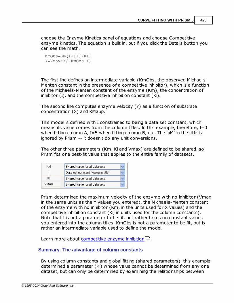
CURVE FITTING WITH PRISM 6 425
© 1995-2014 GraphPad Software, Inc.
choose the Enzyme Kinetics panel of equations and choose Competitiveenzyme kinetics. The equation is built in, but if you click the Details button youcan see the math.
KmObs=Km(1+[I]/Ki)Y=Vmax*X/(KmObs+X)
The first line defines an intermediate variable (KmObs, the observed Michaelis-Menten constant in the presence of a competitive inhibitor), which is a functionof the Michaelis-Menten constant of the enzyme (Km), the concentration ofinhibitor (I), and the competitive inhibition constant (Ki).
The second line computes enzyme velocity (Y) as a function of substrateconcentration (X) and KMapp.
This model is defined with I constrained to being a data set constant, whichmeans its value comes from the column titles. In this example, therefore, I=0when fitting column A, I=5 when fitting column B, etc. The ' M' in the title is
ignored by Prism -- it doesn't do any unit conversions.
The other three parameters (Km, Ki and Vmax) are defined to be shared, soPrism fits one best-fit value that applies to the entire family of datasets.
Prism determined the maximum velocity of the enzyme with no inhibitor (Vmaxin the same units as the Y values you entered), the Michaelis-Menten constantof the enzyme with no inhibitor (Km, in the units used for X values) and thecompetitive inhibition constant (Ki, in units used for the column constants).Note that I is not a parameter to be fit, but rather takes on constant valuesyou entered into the column titles. KmObs is not a parameter to be fit, but israther an intermediate variable used to define the model.
Learn more about competitive enzyme inhibition .
Summary. The advantage of column constants
By using column constants and global fitting (shared parameters), this exampledetermined a parameter (Ki) whose value cannot be determined from any onedataset, but can only be determined by examining the relationships between
345

GraphPad Curve Fitting Guide426
© 1995-2014 GraphPad Software, Inc.
datasets.
2.8.14 Defining equation with two (or more) independent variables
Prism is designed to perform nonlinear regression with one independent (X)variable. But, with a bit of cleverness, it is possible to also fit data with twoindependent variables. There are three separate cases:
Fitting a family of curves
The graph above shows the sample data for competitive enzyme kinetics, andshows how to fit a family of curves. Here, each curve shows enzyme activityas a function of substrate concentration. The curves differ by the presence ofvarious amounts of an inhibitor. There are, essentially, two independentvariables: substrate concentration, and inhibitor concentration.
The substrate concentration is entered into the X column and the inhibitorconcentration into the column titles.

CURVE FITTING WITH PRISM 6 427
© 1995-2014 GraphPad Software, Inc.
When fitting the data, the Constrain tab of the nonlinear regression dialog isused to define the parameter I as dataset constant whose value comes fromthe column titles (so is not fit by regression), and to share the values of all theother parameters so there is one global fit of all the data.
Fitting data where each value has two independent variables
But what if each value you collect has two independent variables? You don'thave a family of curves. Rather you have one set of Y values, each associatedwith two X variables. Follow these steps to enter the data:
1.Create an XY data table, with whatever form of subcolumns fits your data.
2.Enter the first Y value in row 1 of column A.
3.Enter the first independent variable corresponding to that Y into first row ofthe X column.
4.Enter the other independent variable for that first Y value as the column titleof column A.
5.Enter the second Y value in row 2 of column B.
6.Enter the first independent variable for that Y into the second row of the Xcolumn.
7.Enter the other independent variable for that Y as the column title of columnB.
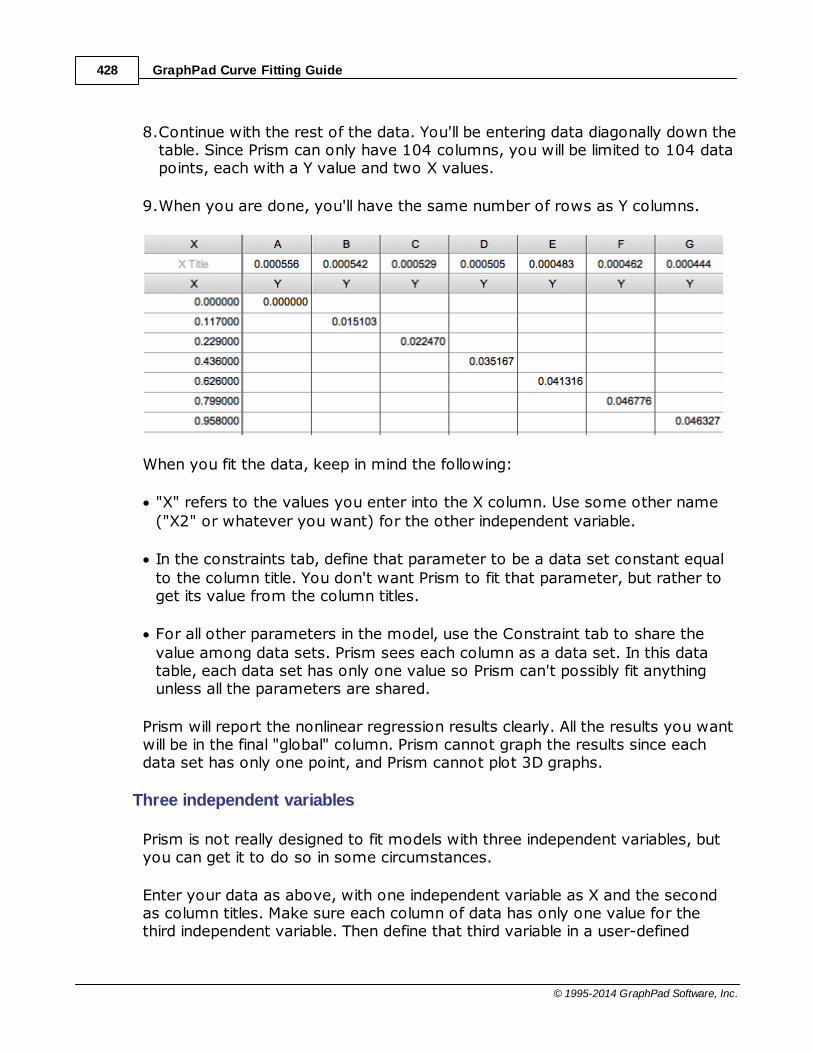
GraphPad Curve Fitting Guide428
© 1995-2014 GraphPad Software, Inc.
8.Continue with the rest of the data. You'll be entering data diagonally down thetable. Since Prism can only have 104 columns, you will be limited to 104 datapoints, each with a Y value and two X values.
9.When you are done, you'll have the same number of rows as Y columns.
When you fit the data, keep in mind the following:
"X" refers to the values you enter into the X column. Use some other name
("X2" or whatever you want) for the other independent variable.
In the constraints tab, define that parameter to be a data set constant equal
to the column title. You don't want Prism to fit that parameter, but rather toget its value from the column titles.
For all other parameters in the model, use the Constraint tab to share the
value among data sets. Prism sees each column as a data set. In this datatable, each data set has only one value so Prism can't possibly fit anythingunless all the parameters are shared.
Prism will report the nonlinear regression results clearly. All the results you wantwill be in the final "global" column. Prism cannot graph the results since eachdata set has only one point, and Prism cannot plot 3D graphs.
Three independent variables
Prism is not really designed to fit models with three independent variables, butyou can get it to do so in some circumstances.
Enter your data as above, with one independent variable as X and the secondas column titles. Make sure each column of data has only one value for thethird independent variable. Then define that third variable in a user-defined

CURVE FITTING WITH PRISM 6 429
© 1995-2014 GraphPad Software, Inc.
equation. Let's imagine that the third variable has the name Z. Add syntax likethis to your equation:
<A> Z=2.34
<B> Z=45.34
<C>Z= -23.4
<D>Z=12.45
That tells Prism to assign Z one value for column A, a different value for columnB, etc. This approach gives you three independent variables, with someconstraints:
The X column is one independent variable, with one value for each row.
The column titles form a second independent variable with one value per data
set column.
The Z values defined within the equation for a third independent variable, also
with one value per data set.
2.8.15 Reparameterizing an equation
Reparameterizing an equation does not change the best-fit curve

GraphPad Curve Fitting Guide430
© 1995-2014 GraphPad Software, Inc.
You want to fit the sigmoidal enzyme kinetics data to a standard model. Butthere are two forms of that model that are commonly used:
Y=Vmax*X^h/(Khalf^h + X^h) Y=Vmax*X^h/(Kprime + X^h)
The two are equivalent, with Kprime equal to Khalfh , so the two fits willgenerate exactly the same curve, with the same sum-of-squares, the same R2,and the same numbers of degrees of freedom. Even though the two equationsexpress the same model, they are written differently. The fancy term is thatthey are parameterized differently.
They both fit Vmax (the maximum activity extrapolated to very highconcentrations of substrate) and h (Hill slope, describing the steepness of thecurve). But one model fits Khalf (the concentration needed to obtain a velocityhalf of maximal) and the other fits Kprime (a more abstract measure ofsubstrate action).
Which model is preferred?
One way to choose between the two models is to match other text books andpapers, so your results can easily be compared to others. Another approach isto choose the form that fits the way you think. For this example, if you preferto think graphically, choose the Khalf. If you think mechanistically, chooseKprime.
But the choice is more than a matter of convenience and convention. Thechoice of model determines the accuracy of the confidence intervals. Read onto see why.
Distribution of parameters are not always symmetrical
GraphPad Prism, like almost all nonlinear regression programs, computes theconfidence interval of a best-fit parameters so the interval is symmetricalaround the best fit values. If the uncertainty of a parameter is trulysymmetrical, then these confidence intervals can be interpreted at face value. Ifthe uncertainty is not symmetrical, then the confidence interval will not beaccurate.
Simulations can determine parameter symmetry. I simulated sigmoidal enzymekinetics using Vmax=100, h=5, Kprime=25, and Gaussian scatter with a SDequal to 7.5. The X values matched those in the figure above, with triplicate Yvalues at each X. Prism can do such simulations easily. Using Prism's MonteCarlo analysis, I repeated the simulations 5000 times, fit each curve to bothforms of the models, and tabulated the best-fit values of Kprime and Khalf, andcomputed the skewness of each.

CURVE FITTING WITH PRISM 6 431
© 1995-2014 GraphPad Software, Inc.
The distribution of Khalf is quite symmetrical and looks Gaussian. Accordingly,its skewness is close to zero. In contrast, the distribution of Kprime is quiteskewed. Note that a few of the simulation data sets had best-fit values ofKprime greater than 100. The skewness value (4.89) confirms what is obviousby inspection -- the distribution is far from symmetrical.
Coverage of the confidence intervals
Ideally, a confidence interval is easy to interpret. A 95% CI has a 95% chanceof including the true value of the parameter, and a 5% chance of missing it.When analyzing real data, we never know the value of the true parameter, sonever know if the interval includes it or not. But when you simulate data, youknow the true values of the parameters, so can quantify the coverage of theconfidence intervals. I set up the same simulations mentioned above, fit eachdata set to both equations, and tabulated whether each confidence intervalincluded the true parameter value or not. This table shows the fraction of 5,000 simulations where the confidence interval did not include the trueparameter value (25 for Kprime, and 1.9037 for Khalf).
"95% CI" "99% CI"
Ideal5.0% 1.0%
Kprime8.8% 4.8%
Khalf5.1% 1.0%
These results show that Khalf is well behaved, as expected given its symmetry

GraphPad Curve Fitting Guide432
© 1995-2014 GraphPad Software, Inc.
(see above). The 95% confidence interval is expected to miss the true value in5.0% of the simulations. In fact, it happened 5.1% of the time. Similarly, the99% CI is expected to miss the true value in 1.0% of the simulations, which isexactly what happened. In contrast, Kprime is less well behaved. The intervalscomputed to be 95% confidence intervals were not wide enough so missed thetrue value in 8.8% of the simulations. The 99% intervals were similarly not wideenough so missed the true value in 4.8% of the simulations. Thus the confidence intervals computed to be 99% intervals, actually turned out to be95% intervals.
These simulations show the advantage of choosing the equation that fits Khalf,rather than the one that fits Kprime. Khalf has a symmetrical distribution so theconfidence intervals computed from these fits can be interpreted at face value.In contrast, Kprime has an asymmetrical distribution and its confidence intervalscannot be interpreted at face value.
Hougaard's skewness
The results above were obtained by running numerous simulations. There is aneasier way to figure out how symmetrical a parameter is. Hougaardsskewness (new in Prism 6) quantifies the asymmetry of each parameter,computed from the equation, the number of data points, the spacing of the Xvalues, and the values of the parameters.
For the simulated data set, Hougaard's skewness is 0.09 for Khalf and 1.83 forKprime. A rule of thumb is to expect problems from asymmetry when theabsolute value of the Hougaard's skewness is greater than 0.25, and bigproblems when the value is greater than 1.0. So Hougaard's skewness tells youthat the confidence intervals will be accurate when you fit Khalf, but not be soaccurate when you fit Kprime.
Note that Hougaard's skewness can be reported as part of the results ofnonlinear regression (choose in the Diagnostics tab). No simulations arerequired.
Bottom line
Models can often be parameterized in multiple ways. You'll get the same curveeither way, but choosing an optimum parameterization ensures that theconfidence intervals for the parameters are believable. The best way to assessvarious parameterizations is to ask Prism to report the value of Hougaardsmeasure of skewness for every parameter. Simulations take a bit more work,but let you see how symmetrical a parameter is.
File used for this example
204
204

CURVE FITTING WITH PRISM 6 433
© 1995-2014 GraphPad Software, Inc.
2.8.16 Rules for initial values
Why initial values?
Before it can perform nonlinear regression, Prism must have initial (estimated)values for each parameter in the equation. It then iteratively modifies thesevalues to improve the fit of the model to the data. The initial values must bereasonable, so that the curve defined by those initial values has generally theshape of the data, and doesn't go awfully far from the data points. If the initialvalues are really bad, Prism may not be able to fit the model.
The need for initial values is not unique to Prism, but is intrinsic to nonlinearregression.
Why rules for initial values?
Prism can store rules (algorithms) to calculate initial values from the range ofyour data. If you choose a built-in equation, the rules are taken care of. If youenter your own (user-defined) equation, you can also enter rules to define theinitial values of each parameter. If you enter a good set of rules, then yourequation will work in the future with no need to think about initial values.
If you don't enter rules for initial values, you will need to enter the initial valuesfor every variable, for every data set, every time you fit data.
If you enter a poor set of rules, then the initial values will not generate a curvethat goes near the data points, and it is likely that Prism will not be able to fitthe model to the data.
How to enter a rule
While entering or editing a user-defined equation, click on the tab labeled "Rulesfor initial values". For each parameter, enter a number in the first column andselect a multiplier from the drop-down list in the second column.

GraphPad Curve Fitting Guide434
© 1995-2014 GraphPad Software, Inc.
Initial value, to be fit
The first choice on the drop-down list is "(Initial value, to be fit)". This meansthat the value you entered in the box to the left will be the initial value for alldata sets. The initial value will not depend on the range of the data (it will not becalculated); it will be the actual value you entered.
Initial value based on the range of the data
Most of the rules are based on the range of the X and Y values.
The abbreviation YMIN is the minimum value of Y; YMAX is the maximum value,and YMID is the average of YMIN and YMAX. For example, if you enter "0.5" inthe first column and select "YMAX" in the second column, Prism sets the initial

CURVE FITTING WITH PRISM 6 435
© 1995-2014 GraphPad Software, Inc.
value to half of YMAX (which differs for each data set).
The phrase "X at YMID" refers to the X value that corresponds to the mean ofthe highest and lowest Y values. Calculation details.
SIGN(YatXmax - YatXmin)
It equals +1 if the curve generally goes up as it goes from left to right: /
It equals -1 if the curve generally goes down as it goes from left to right: \
It is used as the initial value for the Hill Slope in dose response curves.
Here is an explanation of the math. The SIGN() function equals +1 when givena positive number, and -1 when given a negative number. YatXMax is the Yvalue at the largest X values. YatXmin is the Y value at the smallest X value. (YatXmax - YatXmin) will be positive when the curve goes up, and negativewhen the curve goes down.
Mean of column title values (or the log of that mean)
With some kinds of data, it makes sense to label the data sets numerically.Each column titles has a value.
With these kinds of data, you can access the column title values in two ways:
Use the Constrain tab and choose "Data set constant (=column title)". That
parameter in the model is now a constant, but the value of that constant willdiffer for each data set column, and gets it value from the column title.
On the Rules for initial values tab in the dialog that defines an equation, set the
initial value of a parameter to equal the mean of those column titles. Or to thelogarithm of that mean.
The best way to understand this is with an example. Bring up the sample XYdata for competitive enzyme inhibition , and follow the instructions, andinspect the dialog settings.
Example
Y = Vmax*X/(Km + X)
345

GraphPad Curve Fitting Guide436
© 1995-2014 GraphPad Software, Inc.
Km
Vmax
Substrate
Velo
cit
y
The equation above is the Michaelis-Menten enzyme kinetics model built in toPrism. If you pick this equation as a built-in equation, the rules for initial valuesare provided automatically. But if you were entering this as a new user-definedequation, it would be easy to come up with rules.
Vmax is the Y value (enzyme velocity) at very high values of X (substrate). Soa reasonable initial value would be to set Vmax equal to the largest Y value inthe data set. To do this, enter the value 1.0 and choose the multiplier *Ymax.This means Prism will compute the initial value by multiplying the largest Y valueby 1.0. You could argue that Vmax is usually higher than the largest Y value, soshould compute the initial value by multiplying 1.25 times Ymax. There areoften multiple rules one could justify. These rules only compute the initial value,so there is a lot of room for variation.
Km is the X value (substrate concentration) corresponding to a Y value(enzyme velocity) that is half Vmax. Compute its initial value by multiplying 1.0times "Value of X at Ymid". Prism then averages the largest and smallest Yvalues to compute Ymid, and then interpolates from straight connecting lines tofind the corresponding X value.
What happens if you don't enter any rules?
If you don't enter rules for every parameter, Prism will insist that you enterinitial values each time you fit data to the equation.

CURVE FITTING WITH PRISM 6 437
© 1995-2014 GraphPad Software, Inc.
How to override the initial values defined by rule
The rules are stored with each equation, and the rules can be edited as part ofthe dialog that defines and edits equations.
The values defined by the rules are shown in the Initial Value tab of thenonlinear regression dialog. To override the initial values:
1.Select one or several data sets on top of the dialog. Or click "Select all" toselect all data sets.
2.Uncheck the "Choose automatically" option.
3.Enter the initial value (as a value, a number, not a rule) .
To check how good the initial values are, go to the Diagnostics tab and checkthe option:
(*)Don't fit the curve. Instead plot the curve defined by the initial values ofthe parameters.
If the resulting curve doesn't go near the data, revise the initial values (or therules that generate those values) before asking Prism to fit the model to thedata.
2.8.17 Default constraints
What is a constraint?
Constraining parameters is often essential to getting useful results. Constraintscan be used to fix parameters to constant values, to share parametersamong data sets (global fitting), and to define one parameter to be a columnconstant (whose value comes from the column titles in the data table).
Defining constraints when defining an equation
You can define default constraints as part of the equation definition. This isuseful for constraints that will apply every time the equation is used.
Constraints can be for one parameter (Kfast must be greater than zero) or forthe relationship between two parameters (Kfast must be greater than Kslow).But note that you cannot invoke a constraint between two parameters if bothparameters also are themselves constrained. In a two phase exponentialequation, you may want to constrain both parameters to be greater than zero,
158
40
424

GraphPad Curve Fitting Guide438
© 1995-2014 GraphPad Software, Inc.
and also define one rate constant to be larger than the other (Kfast > Kslow).Prism won't let you do that. What you have to do is define one constraint thatKfast is greater than zero, and another that Kfast is greater than Kslow. Butdon't put in the constraint that Kslow is greater than zero. That is implied bybeing larger than Kfast.
Defining experimental constants
In some cases, one of the parameters in the equation is an experimentalconstant. It needs to be set to a constant value, but that value differs eachtime you run the experiment. Do that by going to the constraints tab of thenonlinear regression dialog every time that equation is used.
When you define the equation, you can add a constraint that reminds anyoneusing the equation to set that constant value. In the constraints tab whendefining the equation, choose the constraint "Constant equal to" but leave thevalue (to the right) blank. With an equation defined this way, Prism won't fitdata to that equation until the parameter is defined (or the constraint changed).
2.8.18 Reporting transforms of parameters
When defining an equation, you can also ask Prism to report transforms of thebest-fit values on the "Transforms to report" tab.

CURVE FITTING WITH PRISM 6 439
© 1995-2014 GraphPad Software, Inc.
Transforms of one parameter
Entering the transform
Enter simple transforms of one parameter. On the left side enter the name youwant to give the results. On the right side enter the transform.
Example: You fit data to an equation that includes a parameter logEC50 that isthe logarithm of an EC50, but you want to also report the EC50. Enter the label'EC50' on the left and '10^logEC50' on the right (without the quotes).
Example: You fit data to an equation that reports a rate constant K, but alsowant to report the half-life. Enter the label 'HalfLife' on the left and 'ln(2)/K' onthe right (without the quotes).
Confidence intervals - Symmetrical vs. asymmetrical
When transforming a single parameter, choose between symmetrical andasymmetrical confidence intervals via a drop down to the right of thetransform.
If you choose to report a symmetrical confidence interval, Prism also reportsthe SE of that parameter, and both SE and CI are exactly the same as theywould have been if you had fit that transformed parameter directly. Forexample if you fit an exponential decay model to determine the rate constant,and transform that rate constant (take its reciprocal) to compute the timeconstant, the SE and CI of the time constant will be exactly the same as theywould have been had you fit the time constant directly.

GraphPad Curve Fitting Guide440
© 1995-2014 GraphPad Software, Inc.
If you choose to report an asymmetrical confidence interval, Prism transformsboth confidence limits to create the confidence interval of the transformedparameter. In most cases, this transformed confidence interval will not besymmetrical.
Choosing between the two is often not straightforward. The symmetricalintervals give you the results you would have had if you had chosen to expressthe model differently. The asymmetrical results simply express the sameconfidence interval on a different scale. You want to compute the confidenceintervals on the scale where the true uncertainty is most symmetrical. You canthen transform those confidence limits to come up with asymmetricalconfidence interval on a different scale.
Prism 4 (and earlier) always reported the asymmetrical intervals for EC50 andhalf lives, which were automatically calculated for built-in equations, and did notoffer the choice of transforming parameters in user-defined models.
If your transform simply changes units, then Prism still offers the two choices,but the choice doesn't matter as both end up being exactly the same. This isthe case whenever the transform of parameter K is of the form a*K+b
Interpolating transforms
How to interpolate points off the curve
You can also use these 'transforms' to report values from the curve. Theinterpolated value and its confidence interval will appear in the results, the sameas other transformed parameters.
Use this syntax:

CURVE FITTING WITH PRISM 6 441
© 1995-2014 GraphPad Software, Inc.
Y[value] The Y value of the curve when X is the value you enter withinthe brackets. You must enter a number within the brackets,not a mathematical expression. The Y value will be computedfor any X, but confidence intervals will be calculated only whenthe X value is within the range of the X axis.
X[value] The X value of the curve when Y is the value you enter withinthe brackets. You must enter a number within the brackets,not a mathematical expression. Prism searches for the Y valueyou entered within the range the curve is plotted (Range tab)and extending in each direction a distance equal to half thatrange. It reports the smallest X value it finds within that rangethat corresponds to the Y value you entered, and doesn't alertyou when the curve oscillates so there are several X values ata particular Y value. If both X and Y are within the axis range, aconfidence interval is also calculated.
Example: You fit data to a log(dose) response curve and want to report theantilog of the X value (dose) when Y=50 (which is not always the same as theEC50). For the second example, you would enter "Dose at Y=50' on the left,and '10^X[50]' on the right.
Confidence intervals
The confidence interval for interpolating transforms is computed by interpolationoff the confidence bands of the regression curve. You don't have a choice ofsymmetrical vs. asymmetrical intervals.
Combining two parameters
Usefulness of combining parameters
The bottom half of the tab lets you define combinations of parameters toreport. For example, you can report the sum of two parameters, or the ratio.Enter the name you want to give to the transform on the left, and then choosethe calculation from the drop-down list (say "P1/P2" for a ratio). Then choosewhich parameter is P1 and which is P2 in the drop downs on the right.
Confidence intervals
When Prism combines two parameters to come up with a calculated value, it issmart about propagating the errors. The standard error and confidence intervalit reports for the calculated variable are exactly the same as they would havebeen had you rearranged the equation to directly fit that calculated value.

GraphPad Curve Fitting Guide442
© 1995-2014 GraphPad Software, Inc.
2.9 Plotting a function
Graphing a family of theoretical curves, often called plotting afunction, is useful in three contexts:
To understand the properties of a function. After looking at the
graph, go back and change the parameters to see how the graphchanges. Or plot a family of curves, where one parameter variesfrom curve to curve.
To create graphs for teaching theory.
To understand what initial values would make sense when fitting a
model to data with nonlinear regression.
2.9.1 How to: Plot a function
Prism offers a Plot a function analysis, but it doesn't in fact analyze any data.Rather it generates curves from an equation you choose and parameters youenter.
How to: Plot a function
1.Start from any data table or graph, click Analyze, open the GenerateCurve folder, and then select Plot a function.
2.On the first tab (Function), choose the equation, the starting and endingvalues of X, and the number of curves you want to plot.
3.On the second tab (Options), choose whether you also want to plot thefirst derivative, second derivative or integral of the function. The "curve" isactually a set of X and Y coordinates that define a series of points that areconnected to form the curve. You can choose the number of line segmentsthat will define the curve. There is little reason to change the default (150),unltess you want to plot only a portion of the curve on some graphs, inwhich case you should increase that value.
4.On the third tab (Parameter values), enter the parameter values (or clickthe fish hook icon to hook analysis or info constants).

CURVE FITTING WITH PRISM 6 443
© 1995-2014 GraphPad Software, Inc.
Tips for plotting a function
Plotting a family of curves
If you choose to plot more than one curve (a choice on the first tab), the restof the dialog works a bit differently.
On the bottom of the second (Options) tab, choose if you want to label eachcurve manually (enter the labels the top of the third tab) or using the value ofone of the parameters.
The top of the third tab lists all the curves you will generate. Select one or moreof these curves (or click "select all") and then enter the parameter valuesbelow. Often you'll want to first click "select all" and enter most of theparameters. Then click on one curve at a time, and enter the value for theparameter that varies between curves.
Plotting each curve on a separate graph
By default, Prism will make graph that contains all of the curves on one graph. Ifyou want each curve to be on its on graph, go to the results table, click Newand choose Graph of existing data. On the dialog that pops up, choose to makeone graph for each data set (in this context, a data set is a curve).
If you plan to zoom in and plot only part of the curve
The curve is defined, by default, as 150 line segments. That creates a smoothlooking curve. But if you then change the range of X values shown on thegraph, only a fraction of those line segments will be visible, and the curve mayseem coarse. To fix this problem, go back to the parameters dialog, to theOptions tab, and increase the number of line segments to a much larger value.
Combining two curves on one graph
The graph below combines two plotted functions on one graph. The first time Iplotted a function, I chose a Gaussian distribution, with the X ranging from -3 to3. I set the mean to 0.0, the SD to 1.0, and the amplitude to 100.0 (arbitrary,since I hid that axis). I then repeated that analysis, but this time set the X rangefrom 1.3 to 3.0. I put both curves on one graph (Change.. Add data sets --remember that a curve generated by this analysis is a "data set" to Prism). Forthe shorter curve, I chose to create an area fill.

GraphPad Curve Fitting Guide444
© 1995-2014 GraphPad Software, Inc.
2.9.2 Plotting t, z, F or chi-square distributions
GraphPad Prism can generate probability distributions. This demonstratesPrism's ability to plot functions from user-defined functions, and also the use ofhooking info constants to analyses.
Download this Prism 5 file to generate and plot the graphs shown below.

CURVE FITTING WITH PRISM 6 445
© 1995-2014 GraphPad Software, Inc.
In each case, the simulation generates two (or three) data sets. The first (A)data set plots the entire curve. The equation is written so the second curve(data set B) only plots values where X is less than a specified cutoff value, andthe third curve (data set B) only plots values when X is greater than the cutoffvalue. The second and third data set are plotted with area fill to shade the tailsof the distributions. Remove data set B or C from the graph if you only want toshade one tail. For example, here is the equation used for the first graph (zdistribution):
G=exp(-0.5*X^2)/sqrt(2*3.1415926)<A>Y=G<B>Y=IF(X<-z, G, 0)<C>Y=IF(X>z, G, 0)
Change the numbers of degrees of freedom and the cutoff values (for shading)in the Info sheet. This demonstrates how values entered into an info sheet canbe 'hooked' to constants used in analyses.
2.9.3 Plotting a binomial or Poisson distribution
How to plot a binomial or Poisson distribution
Download the Prism file.
To modify this file, change the value of lamda (for Poission) or the probability,n, and cutoff (Binomial) in the Info sheet. Enter new values there, and the graphupdates. This is a good example of the usefulness of hooking an info constantto an analysis.
If you want to recreate graphs like these, keep in mind these points:
As its name suggests, the analysis 'Create a Family of Theoretical Curves' is
usually used to create curves, not bar graphs. When you choose the range of

GraphPad Curve Fitting Guide446
© 1995-2014 GraphPad Software, Inc.
X values, specify the appropriate number of 'line segments' (points) so thatthe X interval equals 1.0. The binomial example on the left created 16 'linesegments' starting at X=0 and ending at X=15. The Poisson on the rightcreated 13 'segments' with X starting at 0 and ending at 13.
The analysis will create a set of line segments (an attempt to create a curve).
Click the change type of graph button, or drop the Change menu and chooseGraph Type. Then choose the Grouped tab, and then choose interleavedbars.
The binomial example on the right has two data sets. You don't want them
plotted interleaved, as selected in the previous step. Double click to bring upFormat Graph, then go to the middle tab, and choose to superimpose thesecond data set on the first (rather than interleave). And assign it a differentcolor.
Mathematical details
Binomial distribution
The equation for the probability of exactly X successes in N trials, when eachtrial has probability P of success is:
R=INT(X+0.5)ExactProb=(P^R)*(1-P)^(N-R) ;exact probability of successes in n trialsNRearrangments=exp(gammaln(N+1) - gammaln(R+1) - gammaln(N - R +1)) ;gamma(J)=(J-1)factorial, or (J-1)! but factorial is not a function within Prism;NRearrangments = N!/(R! (N-R)!) H=ExactProb * NRearrangments<A>Y=H<B>Y=IF(X>cutoff, H, 0)
Poisson distribution
The equation for the Poisson distribution is:
Y=exp(-1*Lamda)*Lamda^X/gamma(X+1)
Note the definition of the gamma function:
gamma(i) = factorial(i-1) gamma(x+1)= factorial(x) = X!
2.10 Fitting a curve without a model
In some circumstances, your goal is simple. You don't careabout models, and don't expect best-fit values that you can

CURVE FITTING WITH PRISM 6 447
© 1995-2014 GraphPad Software, Inc.
interpret. Instead, you just want to draw a smooth curve tomake a graph look attractive, or to use as a standard curve.
Spline and Lowess curves
Using nonlinear regression with an empiricalmodel
2.10.1 Spline and Lowess curves
Curve fitting without a model
The term curve fitting is more general than regression. Your approach to curvefitting depends on your goal.
In some circumstances, you just want to draw a smooth curve to make agraph look attractive, or to use as a standard curve. You don't care aboutmodels, and aren't looking for best-fit values that you can interpret.
Prism provides two approaches for fitting a curve without selecting a model.From a table or graph of XY data, click Analyze, and then choose 'Fit spline/LOWESS" from the list of XY analyses.
Spline and lowess curves
A lowess curve follows the trend of the data and tends to be a bit jagged.Lowess curves can be helpful when the data progresses monotonically, but areless helpful when there are peaks or valleys. Prism lets you choose betweencoarse, medium and fine lowess curves. The coarse curve (left panel below)shows only the general trend, but obscures the detail. The fine curve (middlepanel below) reveals the fine structure of the data, but tends to wiggle a lot. A cubic spline curve (right panel below) goes through every data point, bendingand twisting as needed.
Prism generates lowess curves using an algorithm adapted from reference 1.
447
448
GraphPad Curve Fitting Guide448
© 1995-2014 GraphPad Software, Inc.
Don't select a lowess curve unless you have well over twenty data points.Prism generates the curve as a series of line segments. Enter the number ofsegments you want, and check the option box if you need to see the XYcoordinates of each point, or if you want to use the resulting lowess, point-to-point, or spline curve as a standard curve. Prism always generates a lowesscurve with at least four times more line segments than the number of datapoints, and you cannot reduce the number of segments below this value.
Creating a point-to-point 'curve'
Prism's spline/lowess analysis can also create a point-to-point "curve" -- aseries of line segments connecting all your data. Don't create a point-to-pointcurve just so you can connect points with a line on the graph. You can do thatby checking an option on the Format Graph dialog from the Graphs section ofyour project. Only select the point-to-point analysis if you want to use thepoint-to-point line as a standard curve, or if you wish to calculate area underthat curve
References
1. John Chambers et. al., Graphical Methods for Data Analysis, Wadsworth andBrooks, 1983.
2.10.2 Using nonlinear regression with an empirical model
If your goal is just to plot a smooth curve, without worrying about a model,you have several choices.
Splines created by Prism go through every point, so may wiggle too much.
Lowess curves follow the general trend of the data, but can be too jagged,
An alternative is to use nonlinear regression.
Nonlinear regression requires you pick a model, but you don't have to payattention to the meaning of the model or the value of the parameters. Instead,you can pick a model empirically and judge it solely on the appearance of thecurve. In this case, you are using nonlinear regression as a tool to create asmooth curve, and not as a method to analyze data.
If you use nonlinear regression in this way, you can experiment with any modelyou want. But first try fitting polynomial models , which are very general (andnever give fitting problems due to poor initial values). If the curve strays too farfrom the trend of the data, pick a higher order model. If the polynomial curvewiggles too much, pick a lower order model.
447
447
381

Index 449
© 1995-2014 GraphPad Software, Inc.
Index- 4 -4PL 256, 262
- 5 -5PL 267
- A -Abolute IC50 248
Adusted R2 216
Advice: How to understand a model 12
AIC 48, 51
AIC. Interpreting. 215
Akaike information criterion 48, 51
Allosteric EC50 shift equation 281
Allosteric modulator defined 311
Allosteric modulator of radioligand binding, equation 322
Ambiguous fits defined 197
Ambiguous nonlinear regression 228
Analysis checklist: Deming regression 103
Analysis checklist: Linear regression 91
Analysis checklist: Nonlinear regression, "Ambiguous" 228
Analysis checklist: Nonlinear regression, "Bad initialvalues" 226
Analysis checklist: Nonlinear regression, "Don't fit" 232
Analysis checklist: Nonlinear regression, "Hitconstraint" 231
Analysis checklist: Nonlinear regression, "Impossibleweights" 233
Analysis checklist: Nonlinear regression, "Interrupted" 226
Analysis checklist: Nonlinear regression, "Notconverged" 227
Analysis checklist: Nonlinear regression, "Perfect fit" 233
Analysis checklist: Nonlinear regression, "Too fewpoints" 232
Analysis checklist: Nonlinear regression, comparingmodels 221
Analysis checklist: Nonlinear regression, general 218
Analysis checklist: Nonlinear regression, interpolating 118, 223
Analysis of Covariance 89
ANCOVA 89
Angled brackets in writing equations 423
Anscome's quartet 18
Association binding experiments 325
Association kinetics (one ligand concentration)equation 328
Association kinetics (two ligand concentrations)equation 329
Association then dissociation, equation 331
Asymmetrical (five parameter) dose-response equation 267
Asymmetrical confidence intervals, nonlinearregression 438
- B -Backfit 104
Bell-shaped dose-response equation 271
Biphasic dose-response equation 269
Boltzmann sigmoid curve 400
Broken line model 374
- C -Centered polynomial equations 381
Cheng and Prusoff 312, 315
Cheng-Prusoff 164
Cloning an equation 409
Colorimetric chemical assays 9
Column constants 424
Compare tab, nonlinear regression 157
Comparing slopes and intercepts: 89
Competitive binding, defined 311
Competitive binding, one site equation 312, 314
Competitive binding, one site, homologous 321
Competitive binding, one site, with ligand depletion 318
Competitive binding, two sites, equation 315, 317
Competitive bindings, equation for kinetics 333
Competitive inhibition of enzyme 345
Complexity, of equations, defined 414
Confidence bands 165
Confidence bands, computation of 67

GraphPad Curve Fitting Guide450
© 1995-2014 GraphPad Software, Inc.
Confidence bands, linear regression 92
Confidence interval of parameters of nonlinearregression 183
Confidence intervals 165
Constrain tab, nonlinear regression 158
Constraints in nonlinear regression, default 437
Convergence criteria 165
Covariance matrix 197
Covariance, analysis of 89
Cox regression 21
Cubic spline 447
Cumulative Gaussian axes, fitting straight lines on 379
Cumulative Gaussian distribution, equation 389
- D -D'Agostino-Pearson normality test of residuals. 185
Damped sine wave 394
Data set constant 158, 424
Deleting equations 410
Deming regression 100
Dependency 197
Depletion of radioligands 289
Diagnostics tab, nonlinear regression 165
Differential equations 414, 415
Dissociation constant, ambiguity 285
Dissociation kinetics equation 326
Don't fit. Nonlinear regression 232
Dose-response curves, defined 235
Dose-response, Five parameters 267
Dose-response, three parameters 255, 256
Dose-shift equation 279
Double exponential decay 360
- E -EC50 defined 236
EC90 283
ECanything 283
Enzyme inhibition, general 337
Enzyme kinetics, assumptions 336
Enzyme progress curve 335
Equation, cloning 409
Equilibrium binding 9
Exponential association equation, one phase 364
Exponential association equation, two phases 367
Exponential decay 9
Exponential decay equation, one phase 357
Exponential decay equation, three phases 362
Exponential decay equation, two phases 360
Exponential decay, derived 356
Exponential defined 355
Exponential growth equation 368
Extra sum-of-squares F test 48
Extra sum-of-squares test 213
- F -F test to compare two models 50
F test, extra sum-of-squares 48
F test, to compare nonlinear fits, interpreting 213
False minimum 206
Family of curves, graphing 442
Fit tab, nonlinear regression 155
Fitting straight lines to semi-log graphs: 376
Fitting two line segments 374
Five parameter dose-response curve 267
Force line through origin 372
Fractional occupancy 285
Functions, graphing 442
- G -Gaddum/Schild EC50 shift equation 277
Gaussian distribution, equation 386
General weighting 31
Generic curves 447
GI50 248, 251
Global nonlinear regression 41
Graphing tips: Linear regression 92
GraphPad radioactivity web calculator 290
- H -Hill slope 240
Hill slope, in saturation binding 300
Hit constraint. Nonlinear regression. 231
Homologous binding defined 311
Hougaard's measure of skewness 204
How the F test works: 50
How to: Linear regression interpolation 76
How to: Linear regression lines 76
How to: Nonlinear regression 126

Index 451
© 1995-2014 GraphPad Software, Inc.
- I -IC50 261, 262, 264, 265
IC50 defined 236
IC50, absolute 248
IC50, relative 248, 251
IC90 283
ICanything 283
IF() statement in segmental regression 421
Implicit equations 414, 416
Impossible weights. Nonlinear regression. 233
Information theory 51
Inhibition of enzymes by substrate 352
Initial rate, in enzyme kinetics 335
Initial values tab 162
Initial values, rules for 433
Intercept of linear regression 84
Interpolating from a standard curve 104
Interrupted nonlinear regression 226
- K -Kcat 340
Kd, meaning of 285
Kinetics of competitive binding, equation 333
Kinetics of radioligand binding 325
Kolmogorov-Smirnov test of residuals 185
- L -Lack of fit, testing for 194
Law of mass action 9, 285
Ligand depletion 289
Linear regression through origin 372
Linear regression, comparing slopes and intercepts 89
Linear regression, goal 14
Linear regression, how it works 15
Linear regression, runs test 90
Linear regression, when to use nonlinear instead 82
Linear vs. nonlinear regression 17
Lines, fitting with nonlinear regression 370
Lineweaver-Burk plot 338
Lineweaver-Burk plots, avoid 19
Local minimum 206
Log Gaussian distribution, equation 388
log((inhibitor) vs. normalized response equation 264
log(agonist) vs. normalized response equation 259
log(agonist) vs. normalized response, equation 258
log(agonist) vs. response -- Variable slope equation 256
log(agonist) vs. response equation 255
log(antagonist) vs. normalized response-- Variableslope equation 265
log(inhibitor) vs. response -- Variable slope equation 262
log(inhibitor) vs. response, equation 261
Logistic curve, four parameter 256, 262
Logistic equation, five parameter 267
Logistic regression 21
Lorentzian distribution, basis for robust regression 59
Lorentzian equation 391
Lowess curve 447
- M -Marquardt method 62
Mass action, law of 285
Mathematical model 9
Michaelis-Menten model 338
Mixed-model inhibition of enzyme 350
Model, defined 9
Models have the same DF 213
Morrison equation of enzyme inhibition 353
Multiple regression 21
- N -Nested models 213
Noncompetitive inhibition of enzyme 347
Nonlinear regression, how it works 62
Nonlinear regression, unequal weighting 30
Nonlinear regression, when to use for fitting a line 82
Nonlinear vs. linear regression 17
Nonspecific binding 288
Normality test, residuals of nonlinear regression 185
Normality tests 165
Normalized data and weighted nonlinear regression 35
Normalized dose-response models 243
Normalizing data, pros and cons 243

GraphPad Curve Fitting Guide452
© 1995-2014 GraphPad Software, Inc.
Normalizing. Does it make sense for dose-responsedata? 241
Not converged. Nonlinear regression. 227
- O -Occupancy of receptor 285
Off rate of radioligand binding 325
On rates of radioligand binding 325
One phase exponential association equation 364
One phase exponential decay equation 357
One site -- Fit total and nonspecific binding, equation 293
One site -- Specific binding equation 297, 300
One site -- Total binding equation 292
One site -- Total, accounting for ligand depletionequation 295
One site competition binding with ligand depletion 318
One site competition equation 312, 314
One site competition homologous competition 321
One site with allosteric modulator equation 309
Operational model. Partial agonists experiments 275
Operational model. Receptor depletion experiments 272
Optical density 9
Origin, forcing a line to go through 372
Orthogonal regression 100
Outlier removal, nonlinear regression 53, 57
Outlier removal, when to avoid 54
Outliers table 207
Outliers, graphing 176
Outliers, what to do when you find one 207
Output tab, nonlinear regression 164
- P -Parallel regression lines, testing for. 89
Perfect fit. Nonlinear regression. 233
Plateau followed by one phase decay, equation 359
Plotting a function 442
Point-to-point 'curve' 447
Poisson weighting 31
Polynomial equations 384
Polynomial regression 21, 381
Power series 404
Prediction bands 165
Prediction bands, computation of 67
Prediction bands, linear regression 92
Probability axes, fitting straight lines on 379
Proportional hazards regression 21
- Q -Q, ROUT coefficient 53, 57
Q, ROUT coefficient, entering 160
Quartet, Anscome 18
- R -R squared, linear regression 86
R2 of weighted fits 65
R2, adjusted 216
R2, nonlinear regression 187
Radioactivity calculations 290
Radioligand binding, ligand depletion 289
Radioligand binding, nonspecific binding 288
Range tab, nonlinear regression 164
Regression through origin 372
Regression, Deming 100
Regression, Orthogonal 100
Regression, use of the term 15
Relative IC50 248, 251
Relative weighting 31
Replicates test 194
Replicates, fitting with nonlinear regression 68
Residual plot, nonlinear regression 179
Residuals from linear regression 92
Residuals, testing normality 165
Robust nonlinear regression 59
Robust nonlinear regression, choosing 155
ROUT coefficient, Q 53, 57
ROUT coefficient, Q, entering 160
ROUT method of identifying outliers 53, 57
Rules for initial values in nonlinear regression 433
Runs test following linear regression 90
Runs test, nonlinear regression 193
- S -Sampling function (sinc wave) 395
Saturation binding, defined 291
Scatchard plots, avoid 19
SD of residuals, from nonlinear regression 187

Index 453
© 1995-2014 GraphPad Software, Inc.
SE of best-fit parameters of nonlinear regression 183
Segmental linear regression 374
Segmental nonlinear regression 421
Semilog graphs, straight lines on 376
Shapiro-Wilk normality test of residuals 185
Sharing parameters 158
Sharing parameters in nonlinear regression 41
Sigmoidal substrate velocity plots 342
Sinc wave 395
Sine wave 393
Sine wave, damped 394
Skewness of nonlinear regression parameter 204
Slope factor 240
Slope of linear regression 84
Slope, testing if is really zero 88
Sorting equations 410
Specific binding, defined 291
SSreg, from nonlinear regression 187
Standard curve, interpolating 104
Standard errors 165
Steady state, in enzyme kinetics 335
Substrate inhibition of enzymes 352
Summary table, nonlinear regression 164
Sum-of-squares, why minimize 61
sy.x, from nonlinear regression 187
Symmetrical confidence intervals, nonlinear regression 438
- T -Theoretical curves, graphing 442
Three parameter dose-response curve 255, 256
Three phase exponential decay equation 362
Tight inhibition of enzymes 353
Too complex, defined 414
Too few points. Nonlinear regression 232
Transforms of best-fit values of parameters of nonlinearregreseson 438
Two phase exponential association equation 367
Two phase exponential decay equation 360
Two site competition equation 315, 317
Two sites -- Fit total and nonspecific binding, equation 307
Two sites -- Specific binding only, equation 304
- U -Uncompetitive inhibition of enzyme 349
Unequal weighting 160
User-defined equations 411
- V -Variable slope vs. fixed slope, dose-response 241
- W -Weighted nonlinear regression, normalized data 35
Weighted residuals 179
Weighting in nonlinear regression, implementation 65
Weighting in nonlinear regression, math 31
Weighting in nonlinear regression, outliers 65
Weighting in nonlinear regression, R2 65
Weighting in robust regression 65
Weighting, general 31
Weighting, nonlinear regression 30
Weighting, Poisson 31
Weighting, relative 31
Weights tab, nonlinear regression 160