Type Curve Analysis Type Curve Analysis Type Curve Analysis Type Curve Analysis
53
Type Curve Analysis Type Curve Analysis Type Curve Analysis Type Curve Analysis
Transcript of Type Curve Analysis Type Curve Analysis Type Curve Analysis Type Curve Analysis

Type Curve AnalysisType Curve AnalysisType Curve AnalysisType Curve Analysis

T C A l iT C A l iType Curve AnalysisType Curve AnalysisInstructional ObjectivesInstructional ObjectivesInstructional ObjectivesInstructional Objectives
1.1. Identify wellbore storage and middle time regions Identify wellbore storage and middle time regions on type curve.on type curve.
2.2. Identify pressure response for a well with high, zero, Identify pressure response for a well with high, zero, or negative skin.or negative skin.
3.3. Calculate equivalent time.Calculate equivalent time.4.4. Calculate wellbore storage coefficient, permeability, Calculate wellbore storage coefficient, permeability,
and skin factor from type curve match. and skin factor from type curve match.

Dimensionless VariablesDimensionless Variables

Dimensionless Variables
rcEiqBpp t
2948670
ktEi
khpp t
i 6.70
2 D
rr
2
1 wi rr
Eippkhw
D r
2
0002637.0422.141
wtrckt
EiqB
qBppkhp i
D 2.141
2
0002637.0D rc
ktt
D
DrEip42
1 2
qwtrc
D
D tp
42

Dimensionless VariablesDimensionless VariablesRadial Flow With WBS And SkinRadial Flow With WBS And Skin
ppkhp i 0002637.0
Dktt
qBpD 2.141
2wt
D rct
wD r
rr w
qBpkhs s
2141 2
8936.0D hrc
CC
qB2.141 wthrc

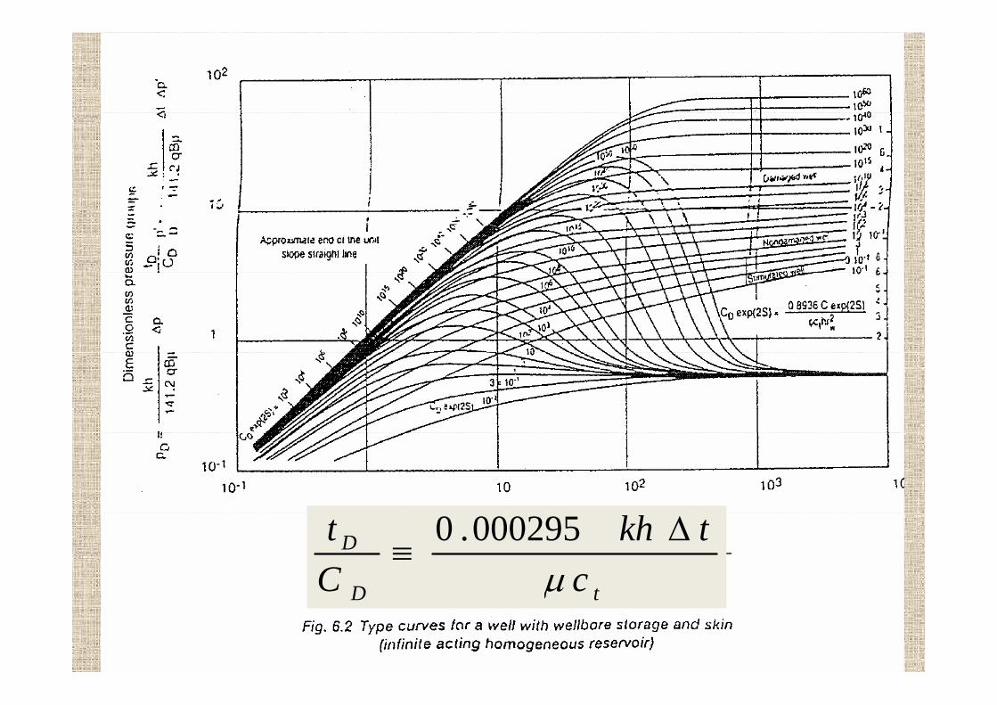
GringartenGringarten T pe C r eT pe C r eGringartenGringarten Type CurveType Curve
•• Constant rate productionConstant rate production•• Vertical wellVertical well•• Vertical wellVertical well•• InfiniteInfinite‐‐acting homogeneous reservoiracting homogeneous reservoir•• SingleSingle‐‐phase, slightly compressible liquidphase, slightly compressible liquid•• Infinitesimal skin factorInfinitesimal skin factor•• Infinitesimal skin factorInfinitesimal skin factor•• Constant wellbore storage coefficientConstant wellbore storage coefficient
GringartenGringarten Type CurvesType Curvesgg ypypinfinite acting homogenous reservoirinfinite acting homogenous reservoir
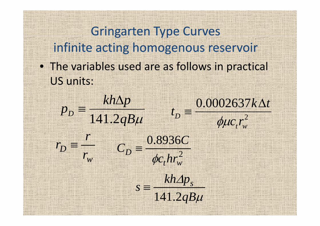
• The variables used are as follows in practical US units:
pkhpD
0002637.0 tkt qB
pD 2.141 2wt
D rct
r 89360 Cw
D rrr
28936.0
wtD hrc
CC
pkhs s
wt
qBs
2.141

D
D
ctkh
Ct
000295.0
tD cC
GringartenGringarten TypeType CurveCurve (cont )(cont )GringartenGringarten Type Type CurveCurve (cont.)(cont.)
• The Gringarten type curve was specifically developed for drawdown tests in oil wells. pWe will see that we may use it (with some limitations) to analyze pressure builduplimitations) to analyze pressure buildup tests in addition to drawdown tests, and to analyze gas well tests as well as oil wellanalyze gas well tests as well as oil well tests.

GringartenGringarten TypeType CurveCurve (cont )(cont )
I th G i t t th ti i
GringartenGringarten Type Type CurveCurve (cont.)(cont.)
• In the Gringarten type curve, the time is plotted as tD/CD, and the dimensionless wellbore storage coefficient and the skin factor are combined into a parameter CDe2s.
• Each value of the parameter CDe2s
describes a pressure response having adescribes a pressure response having a different shape.

Pressure Type CurvePressure Type Curve100 CDe2s=1060
10 CDe2s=100
1D 1p D
C e2s=0 010.1
CDe2s=0.01
0.010 01 0 1 1 10 100 1000 10000 1000000.01 0.1 1 10 100 1000 10000 100000
tD/CD

Pressure DerivativePressure DerivativePressure DerivativePressure Derivative
s
rckt
khqBp
wt869.023.3log6.162
2
ppt DD ppt tp
tpt
ln
D
D
D
DD t
ptpt
ln
qBpt 6.70
5.0 D
Dpt
kht DD t

Derivative TypeDerivative Type CurveCurve
If l l t th “l ith i d i ti ” f thIf l l t th “l ith i d i ti ” f th
Derivative Type Derivative Type CurveCurve
•• If we calculate the “logarithmic derivative” of the If we calculate the “logarithmic derivative” of the semilogsemilog approximation to the line source solution, approximation to the line source solution, we find that the result is a constant that dependswe find that the result is a constant that dependswe find that the result is a constant that depends we find that the result is a constant that depends on flow rate, fluid properties, and rock properties.on flow rate, fluid properties, and rock properties.
•• The logarithmic derivative of the dimensionless The logarithmic derivative of the dimensionless form of the same equation is a constant with theform of the same equation is a constant with theform of the same equation is a constant with the form of the same equation is a constant with the value 0.5.value 0.5.
•• Note that the logarithmic derivative of pressure Note that the logarithmic derivative of pressure has the same units as pressure.has the same units as pressure.pp

Derivative Type Derivative Type CurveCurve (cont.)(cont.)yy ( )( )100
CCDDee2s2s=10=106060
10
CCDDee2s2s=100=100
1p D'
1
t Dp
CCDDee2s2s=0.01=0.010.1
0.010 01 0 1 1 10 100 1000 10000 1000000.01 0.1 1 10 100 1000 10000 100000
tD/CD

Pressure And Derivative Type CurvesPressure And Derivative Type Curvesypyp100
10
1Dp D
'
1
p D, t
D
0.1
0.010 01 0 1 1 10 100 1000 10000 1000000.01 0.1 1 10 100 1000 10000 100000
tD/CD

Derivative TypeDerivative Type CurveCurve (cont )(cont )Derivative Type Derivative Type CurveCurve (cont.)(cont.)
•• Just as we constructed a dimensionless type Just as we constructed a dimensionless type curve with different stems corresponding to curve with different stems corresponding to different values of Cdifferent values of CDDee2s2s, we can construct a , we can construct a derivative type curve from the logarithmic derivative type curve from the logarithmic yp gyp gderivative of the pressure type curve.derivative of the pressure type curve.
•• The shapes of these stems are much more The shapes of these stems are much more di ti ti th th f th tdi ti ti th th f th tdistinctive than those for the pressure type distinctive than those for the pressure type curve.curve.
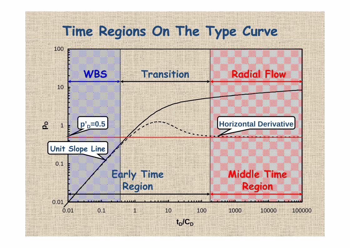
Time Regions On The Type CurveTime Regions On The Type Curve100
10
WBS Transition Radial Flow
1D Horizontal Derivativep’ =0 51p D
Unit Slope Line
Horizontal Derivativep D=0.5
0.1
Middle Time Early Time
p
0.010 01 0 1 1 10 100 1000 10000 100000
Regiony
Region
0.01 0.1 1 10 100 1000 10000 100000
tD/CD

Early TimesEarly TimesEarly TimesEarly Times
E h f th t th G i t t• Each of the stems on the Gringarten type curve exhibits characteristic behavior.
• At early times, the pressure and pressure derivative fall on a unit-slope line. During p gthis period, the pressure response is completely determined by the wellbore co p ete y dete ed by t e e bo eproperties. Permeability cannot be estimated if the only data available liesestimated if the only data available lies within this WBS-dominated period.
Middle Time RegionMiddle Time RegionMiddle Time RegionMiddle Time Region
• After WBS effects have ceased, the derivative follows a horizontal line. This is referred to as the “middle time region”. Permeability may be estimated wheneverPermeability may be estimated whenever there is 1/2 log cycle or more of data in the middle time regionmiddle time region.

Transition PeriodTransition PeriodTransition PeriodTransition Period
• There is a transition period between the unit slope line and the middle time region. p gDuring this transition, both WBS and reservoir properties influence the pressurereservoir properties influence the pressure response. It is sometimes possible to estimate permeability using data duringestimate permeability using data during WBS and the transition, but the results are not as reliable as when there is data lying in the middle time regiong

Estimating Skin FactorEstimating Skin Factor100
High Skin
10
1Dp D
' No Skin
1
p D, t
D
0.1Negative Skin
0.010 01 0 1 1 10 100 1000 10000 1000000.01 0.1 1 10 100 1000 10000 100000
tD/CD

Skin FactorSkin FactorSkin FactorSkin Factor•• Skin factor may be estimated qualitatively by theSkin factor may be estimated qualitatively by the•• Skin factor may be estimated qualitatively by the Skin factor may be estimated qualitatively by the
shape of the pressure and pressure derivative shape of the pressure and pressure derivative responseresponseresponse.response.
•• High skin factorHigh skin factor•• The pressure derivative rises to a maximum and then The pressure derivative rises to a maximum and then
falls sharply before flattening out for the MTR.falls sharply before flattening out for the MTR.Th i l it l thTh i l it l th•• The pressure curve rises along a unit slope then The pressure curve rises along a unit slope then flattens out quickly.flattens out quickly.
•• The pressure and pressure derivative are separatedThe pressure and pressure derivative are separated•• The pressure and pressure derivative are separated The pressure and pressure derivative are separated by ~2 log cycles after the end of WBS.by ~2 log cycles after the end of WBS.
Skin FactorSkin FactorSkin FactorSkin Factor
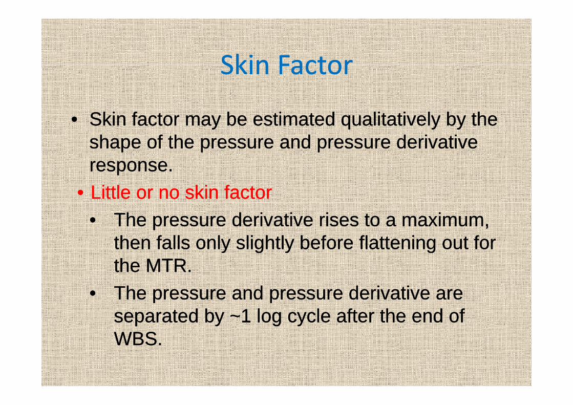
•• Skin factor may be estimated qualitatively by the Skin factor may be estimated qualitatively by the shape of the pressure and pressure derivative shape of the pressure and pressure derivative response.response.
•• Little or no skin factorLittle or no skin factor•• The pressure derivative rises to a maximum, The pressure derivative rises to a maximum,
then falls only slightly before flattening out forthen falls only slightly before flattening out forthen falls only slightly before flattening out for then falls only slightly before flattening out for the MTR.the MTR.
•• The pressure and pressure derivative areThe pressure and pressure derivative are•• The pressure and pressure derivative are The pressure and pressure derivative are separated by ~1 log cycle after the end of separated by ~1 log cycle after the end of WBSWBSWBS.WBS.
Skin FactorSkin FactorSkin FactorSkin Factor
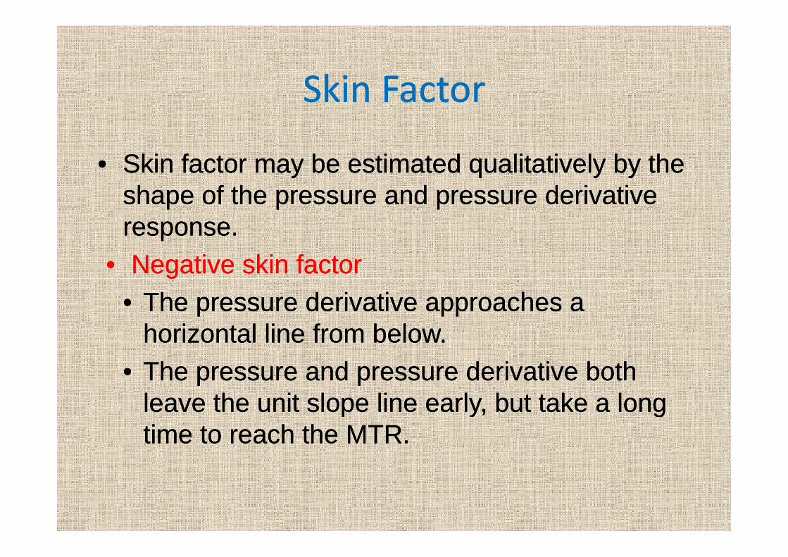
•• Skin factor may be estimated qualitatively by the Skin factor may be estimated qualitatively by the shape of the pressure and pressure derivative shape of the pressure and pressure derivative response.response.
•• Negative skin factorNegative skin factorgg•• The pressure derivative approaches a The pressure derivative approaches a
horizontal line from below.horizontal line from below.horizontal line from below.horizontal line from below.•• The pressure and pressure derivative both The pressure and pressure derivative both
leave the unit slope line early but take a longleave the unit slope line early but take a longleave the unit slope line early, but take a long leave the unit slope line early, but take a long time to reach the MTR.time to reach the MTR.

llEquivalent Time For PBU TestsEquivalent Time For PBU Tests
sktqBpp 8690233loglog6162
src
tkh
ppwt
pwfi 869.023.3loglog6.162 210
skttqBpp 8690233loglog6162
kqB
src
ttkh
ppwt
pwsi 869.023.3loglog6.162 210
s
rckt
khqB
wt869.023.3loglog6.162 210

Equivalent Time For PBU TestsEquivalent Time For PBU TestsEquivalent Time For PBU TestsEquivalent Time For PBU Tests
s
rckt
khqBpp
wtpwfws 869.023.3loglog6.162 210
s
rcktt
khqB
wtp 869.023.3loglog6.162 210
sktkh
qB
rc wt
869.023.3loglog6.162 210
rckh wt
gg 210
s
rck
tttt
khqBpp p
wfws 869.023.3loglog6.162 210
rcttkh wtp
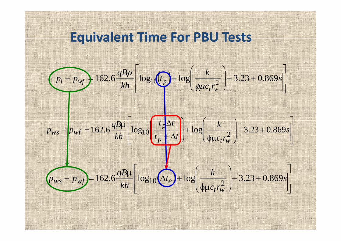
Equivalent Time For PBU TestsEquivalent Time For PBU TestsEquivalent Time For PBU TestsEquivalent Time For PBU Tests
s
rckt
khqBpp
wtpwfi 869.023.3loglog6.162 210
s
rck
tttt
khqBpp
wtp
pwfws 869.023.3loglog6.162 210
kqB 8690233ll6162
src
ktkh
qBppwt
ewfws 869.023.3loglog6.162 210

E i l t Ti F PBU T tE i l t Ti F PBU T tEquivalent Time For PBU TestsEquivalent Time For PBU Tests
Drawdown wfi ppp vs t
Buildup wfws ppp vs et

Properties Of Equivalent TimeProperties Of Equivalent TimeProperties Of Equivalent TimeProperties Of Equivalent Time
tt tt
ttt
p
pe
tt p
pttt ,tt p
t
pttt ,
pp
ttt
t
pp ttt ,
t pHTR
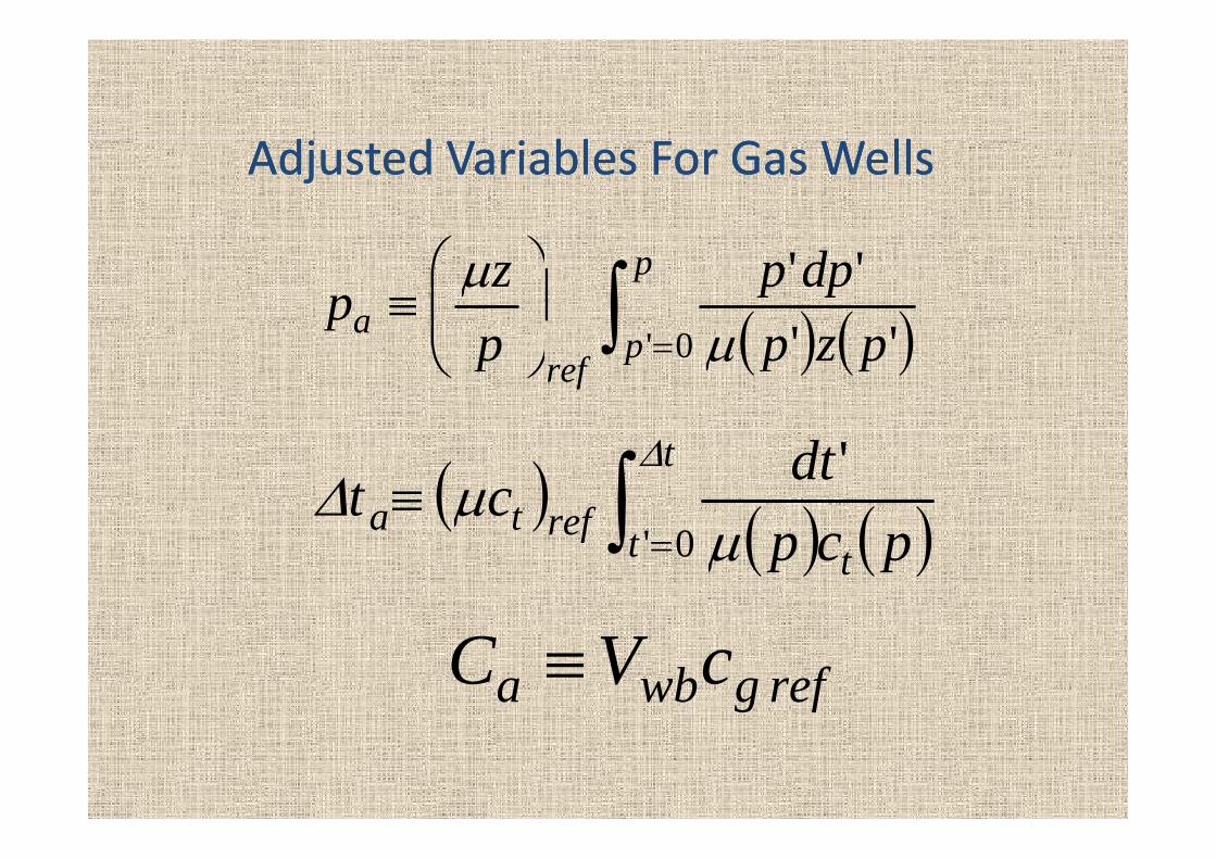
Adjusted Variables For Gas WellsAdjusted Variables For Gas Wells
pa
dppzp''
''
p
refa pzpp 0' ''
t
reftadtct
' t t
refta pcp
0'
refgwba cVC

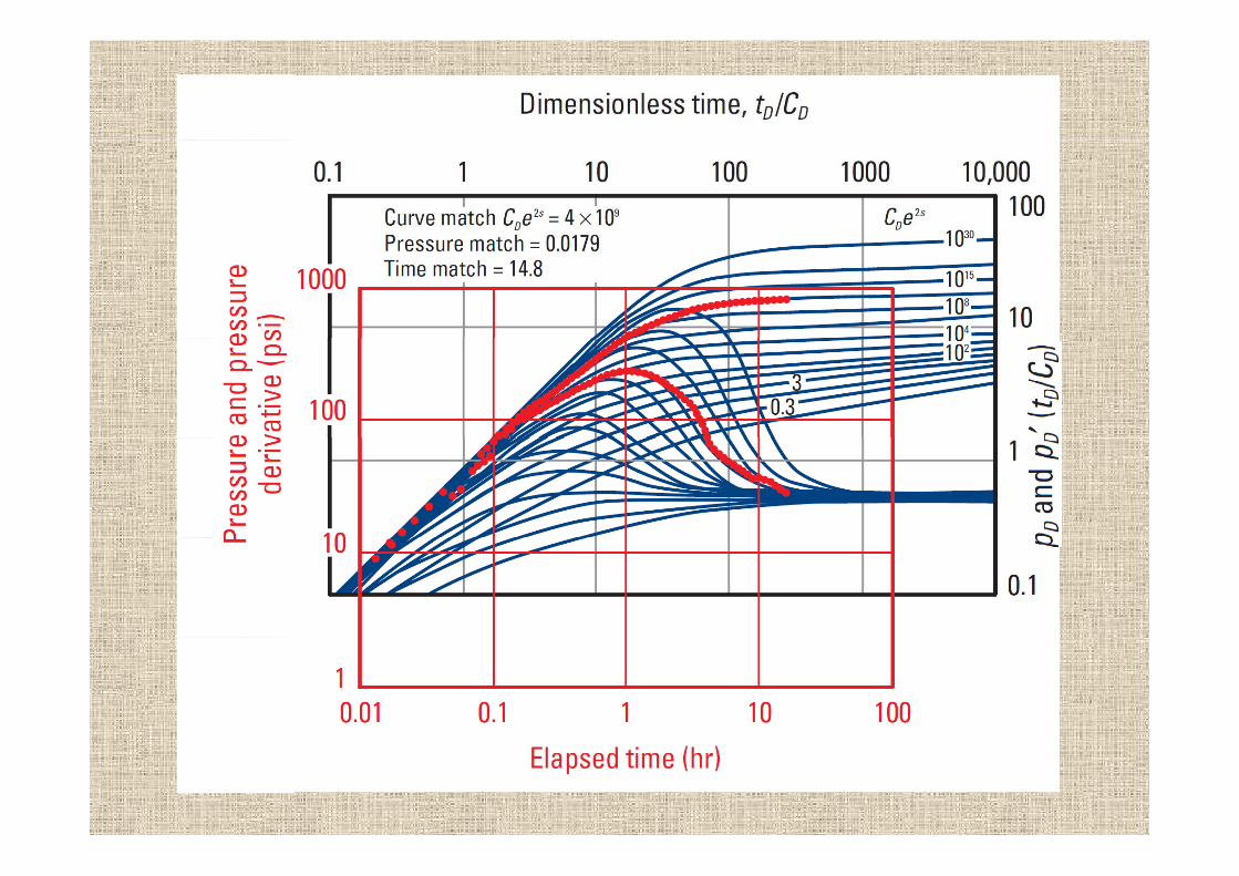
Type Curve MatchingType Curve Matchingyp gyp g
•• Plot field data on logPlot field data on log‐‐log scalelog scale•• Align horizontal part of field data and typeAlign horizontal part of field data and typeAlign horizontal part of field data and type Align horizontal part of field data and type curve derivativecurve derivativeAli i l f fi ld d dAli i l f fi ld d d•• Align unit slope part of field data and type Align unit slope part of field data and type curvecurve
•• Select value of CSelect value of CDDee2s2s that best matches field that best matches field datadatadatadata
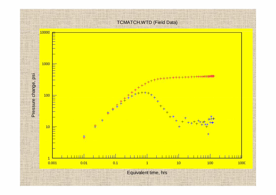
TCMATCH.WTD (Field Data)
1000010000
1000
si
100chan
ge, p
sP
ress
ure
10
10.001 0.01 0.1 1 10 100 10000.001 0.01 0.1 1 10 100 1000
Equivalent time, hrs
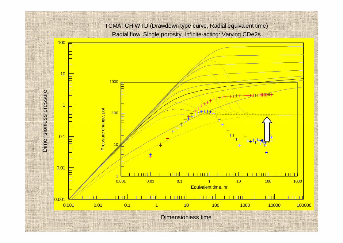
TCMATCH.WTD (Drawdown type curve, Radial equivalent time)Radial flow, Single porosity, Infinite-acting: Varying CDe2s
100
10
re
1000
1
ess
pres
sur
100
nge,
psi
0.1
Dim
ensi
onle
10
Pre
ssur
e ch
an
0.01
D
1
P
0.0010 001 0 01 0 1 1 10 100 1000 10000 100000
0.001 0.01 0.1 1 10 100 10001
Equivalent time, hr
0.001 0.01 0.1 1 10 100 1000 10000 100000
Dimensionless time
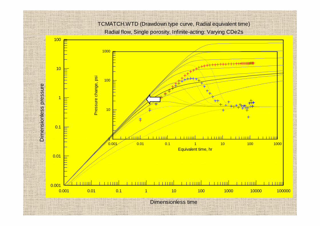
TCMATCH.WTD (Drawdown type curve, Radial equivalent time)Radial flow, Single porosity, Infinite-acting: Varying CDe2s
100
1000
10
re
100
ge, p
si1
ess
pres
sur
10
Pre
ssur
e ch
ang
0.1
Dim
ensi
onle
1
P
0.01
D
0.001 0.01 0.1 1 10 100 10001
Equivalent time, hr
0.0010 001 0 01 0 1 1 10 100 1000 10000 1000000.001 0.01 0.1 1 10 100 1000 10000 100000
Dimensionless time
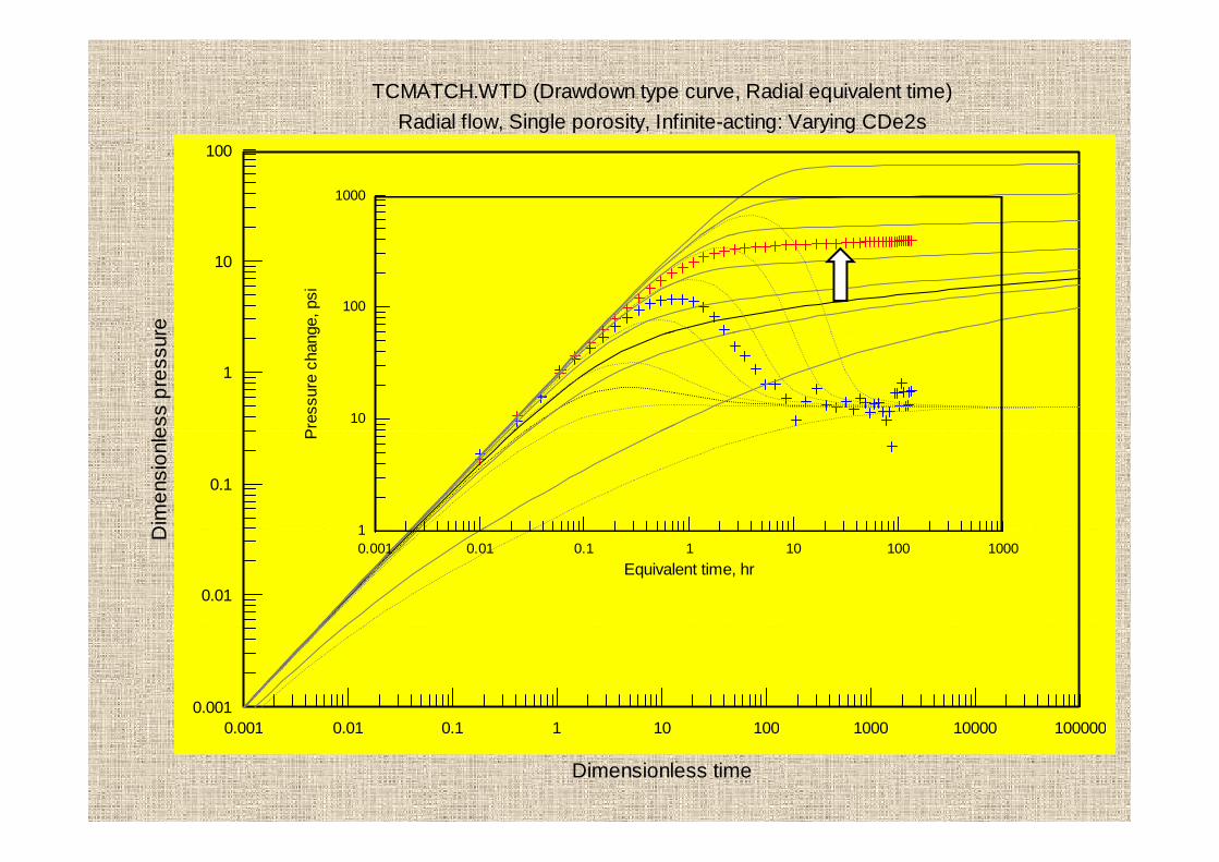
TCMATCH.WTD (Drawdown type curve, Radial equivalent time)Radial flow, Single porosity, Infinite-acting: Varying CDe2s
100
1000
10
re
100ge
, psi
1
ess
pres
sur
10
Pre
ssur
e ch
ang
0.1
Dim
ensi
onle
1
P
0.01
D
0.001 0.01 0.1 1 10 100 10001
Equivalent time, hr
0.0010 001 0 01 0 1 1 10 100 1000 10000 1000000.001 0.01 0.1 1 10 100 1000 10000 100000
Dimensionless time
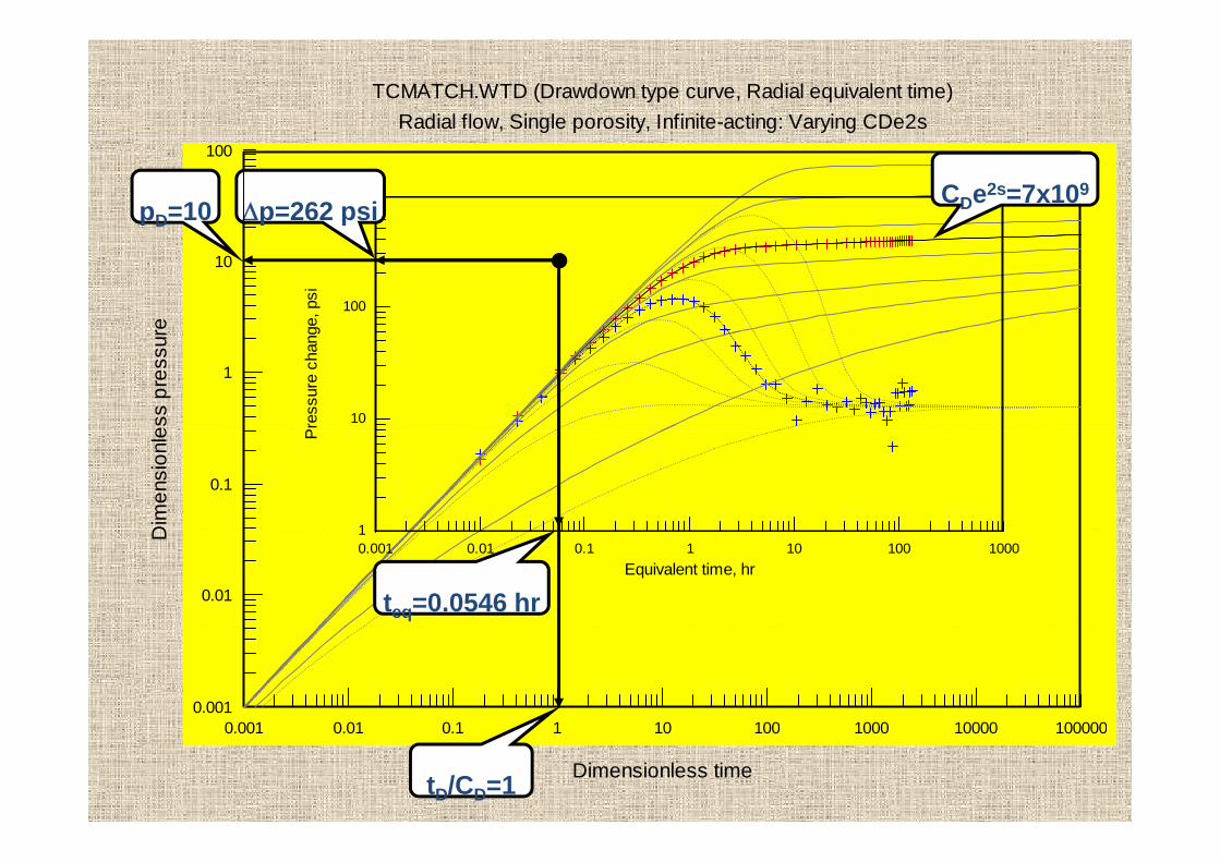
TCMATCH.WTD (Drawdown type curve, Radial equivalent time)Radial flow, Single porosity, Infinite-acting: Varying CDe2s
100
1000p=262 psipD=10 CDe2s=7x10⁹
10
re
100ge
, psi
1
ess
pres
sur
10
Pre
ssur
e ch
ang
0.1
Dim
ensi
onle
1
P
0.01
D
0.001 0.01 0.1 1 10 100 10001
Equivalent time, hr
teq=0.0546 hr
0.0010 001 0 01 0 1 1 10 100 1000 10000 1000000.001 0.01 0.1 1 10 100 1000 10000 100000
Dimensionless timetD/CD=1

Interpreting Type Curve MatchInterpreting Type Curve MatchInterpreting Type Curve MatchInterpreting Type Curve Match
•• Calculate k from the pressure match Calculate k from the pressure match point ratiopoint ratio p/p/pppoint ratio point ratio p/p/ppDD
•• Calculate CCalculate CDD from the time match pointfrom the time match pointCalculate CCalculate CDD from the time match point from the time match point ratio ratio tteqeq//ttDD
•• Calculate s from the matching stem value Calculate s from the matching stem value CCDDee2s2sCCDDee

CalculateCalculate kk From PressureFrom PressureCalculate Calculate kk From Pressure From Pressure MatchMatch2.141 DpqBk
..PM
D
pp
hqk
1060903251502141 k
26210
15609.0325.1502.141
md5.14
26215

Calculate Calculate CCDD From Time MatchFrom Time Match
0002637.0 eqtkC
..
2PMDDwt
D CtrcC
0546051400026370 1
0546.025.01076.1609.0183.0
5.140002637.05
DC
1703

22Calculate Calculate ss From From CCDDee2s2s
s
DeC 2l1
D
D
CeCs ln
21
1071 9
1703107ln
21 9
s
6.7
17032
6.7

BOURDET TYPE CURVES FOR A WELLBORE STORAGE AND SKIN, BOURDET TYPE CURVES FOR A WELLBORE STORAGE AND SKIN, DOUBLE POROSITY BEHAVIOUR DOUBLE POROSITY BEHAVIOUR
((PSEUDOSTEADYPSEUDOSTEADY‐‐STATE REGIME BETWEEN THE TWO POROSITY SYSTEMSSTATE REGIME BETWEEN THE TWO POROSITY SYSTEMS))
tD
D
ctkh
Ct
000295.0
tD
D
ctkh
Ct
000295.0
tD
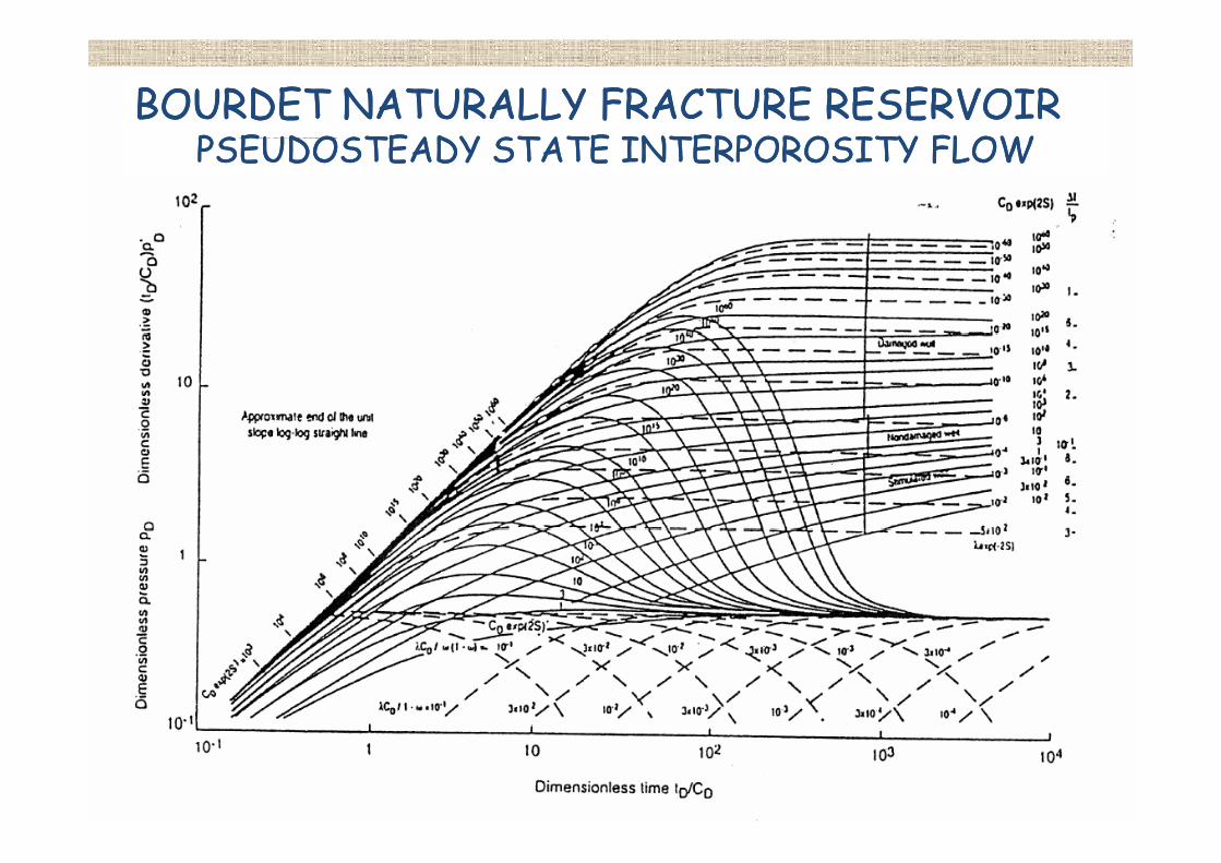
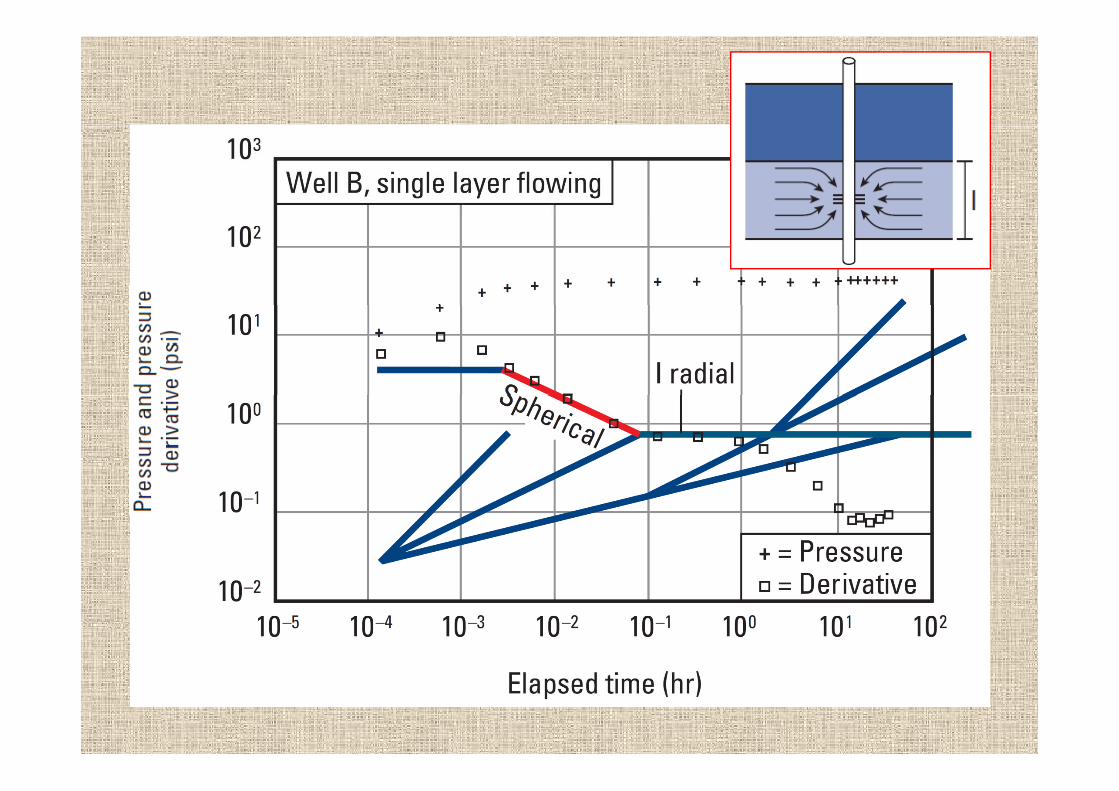
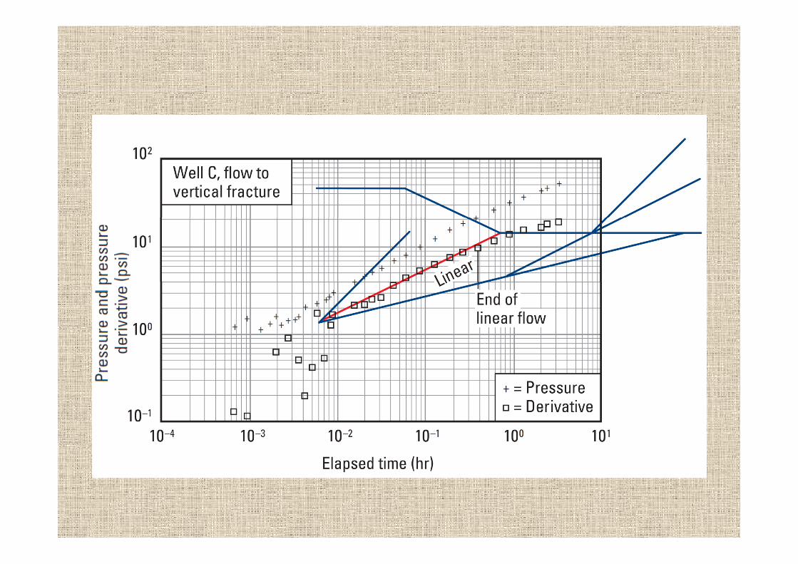
BOURDET NATURALLY FRACTURE RESERVOIR BOURDET NATURALLY FRACTURE RESERVOIR PSEUDOSTEADY STATE INTERPOROSITY FLOWPSEUDOSTEADY STATE INTERPOROSITY FLOWPSEUDOSTEADY STATE INTERPOROSITY FLOWPSEUDOSTEADY STATE INTERPOROSITY FLOW

BOURDET NATURALLY FRACTURE RESERVOIRBOURDET NATURALLY FRACTURE RESERVOIRTRANSIENT INTERPOROSITY FLOW


Plot of the Plot of the bottomholebottomhole flow rate and pressure flow rate and pressure recorded during a drawdown testrecorded during a drawdown testrecorded during a drawdown test.recorded during a drawdown test.
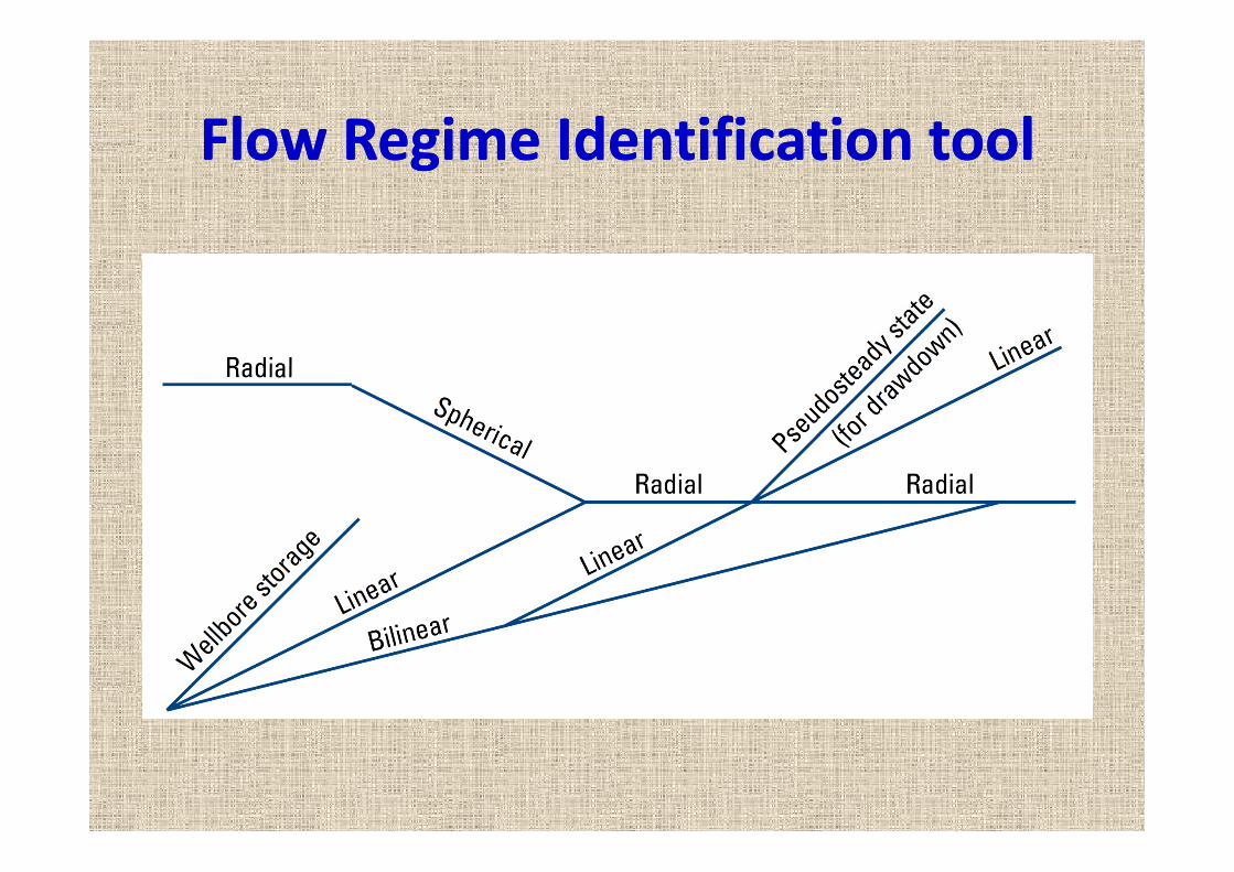
Flow Regime Identification toolFlow Regime Identification toolFlow Regime Identification toolFlow Regime Identification tool