(A) QUES. DESCRIBE CHARACTERISTICS

OF NORMAL PROBABLITY CURVE (NPC)

INTRODUCTION: -

A normal curve is a bell-shaped curve which shows the probability

distribution of a continuous random variable. Moreover, the normal

curve represents a normal distribution. The total area under the

normal curve logically represents the sum of all probabilities for a

random variable. Hence, the area under the normal curve is one. Also,

the standard normal curve represents a normal curve with mean 0 and

standard deviation 1. Thus, the parameters involved in a normal

distribution is mean ( μ ) and standard deviation ( σ ).

The “Graph of the probability density function of the normal

distribution is a continuous bell shaped curve, symmetrical about

the mean” is called Normal Probability Curve.

In statistics it is important because:

(а) It is the distribution of many naturally occurring variables, such as

intelligence of 8th grade students, height of the 10th grade students

etc.

(b) The distribution of the means of samples drawn from most parent

populations is normal or approximately so when the samples are

sufficiently large.

Therefore normal curve has great significance in social sciences and

behavioural sciences. In behavioural measurement most of the aspects

approximates to the normal distribution.

So that Normal Probability Curve or most popularly known as

NPC is used as a reference curve. In order to understand the utility of

the NPC we must have to understand the properties of the NPC.

Characteristics of Normal Probability Curve

Some of the major characteristics of normal probability curve are

as follows:

1. The normal curve is symmetrical:

The Normal Probability Curve (N.P.C.) is symmetrical about the

ordinate of the central point of the curve. It implies that the size,

shape and slope of the curve on one side of the curve is identical to

that of the other.

That is, the normal curve has a bilateral symmetry. If the figure is to

be folded along its vertical axis, the two halves would coincide. In

other words the left and right values to the middle central point are

mirror images.

fig. 1

2. The normal curve is unimodal:

Since there is only one point in the curve which has maximum

frequency, the normal probability curve is unimodal, i.e. it has only

one mode.

3. Mean, median and mode coincide:

The mean, median and mode of the normal distribution are the same

and they lie at the centre. They are represented by 0 (zero) along the

base line. [Mean = Median = Mode]

4. The maximum ordinate occurs at the centre:

The maximum height of the ordinate always occurs at the central

point of the curve that is, at the mid-point. The ordinate at the mean is

the highest ordinate and it is denoted by Y0. (Y0 is the height of the

curve at the mean or mid-point of the base line).

5. The normal curve is asymptotic to the X-axis:

The Normal Probability Curve approaches the horizontal axis

asymptotically i.e., the curve continues to decrease in height on both

ends away from the middle point (the maximum ordinate point); but it

never touches the horizontal axis.

It extends infinitely in both directions i.e. from minus infinity (-∞) to

plus infinity (+∞) as shown in Figure below. As the distance from the

mean increases the curve approaches to the base line more and more

closely.

fig. 2 Normal Curve is Asymptotic to X-axis

6. The height of the curve declines symmetrically:

In the normal probability curve the height declines symmetrically in

either direction from the maximum point. Hence the ordinates for

values of X = µ ± K, where K is a real number, are equal.

For example:

The heights of the curve or the ordinate at X = µ + σ and X = µ –

σ are exactly the same as shown in the following Figure:

Fig. 3 The Ordinates of a Normal Curve

7. The points of Influx occur at point ± 1 Standard Deviation (± 1

a):

The normal curve changes its direction from convex to concave at a

point recognized as point of influx. If we draw the perpendiculars

from these two points of influx of the curve on horizontal axis, these

two will touch the axis at a distance one Standard Deviation unit

above and below the mean (± 1 σ).

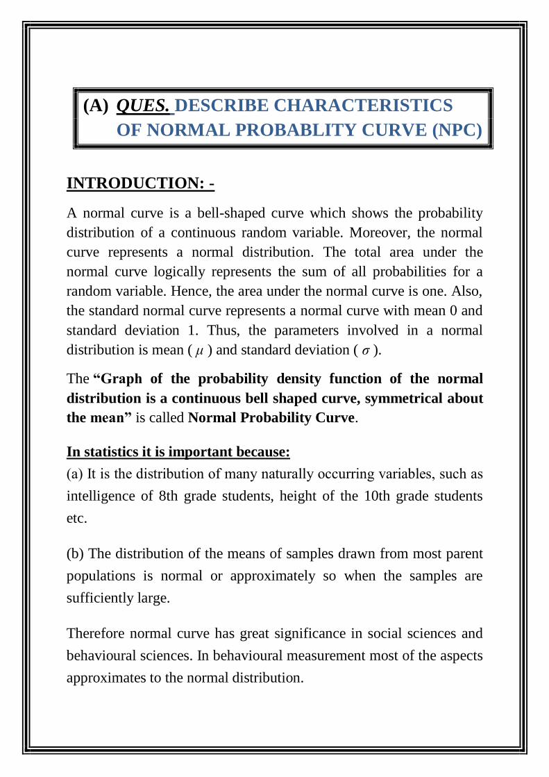
8. The total percentage of area of the normal curve within two

points of influxation is fixed:

Approximately 68.26% area of the curve falls within the limits of ±1

standard deviation unit from the mean as shown in figure below.

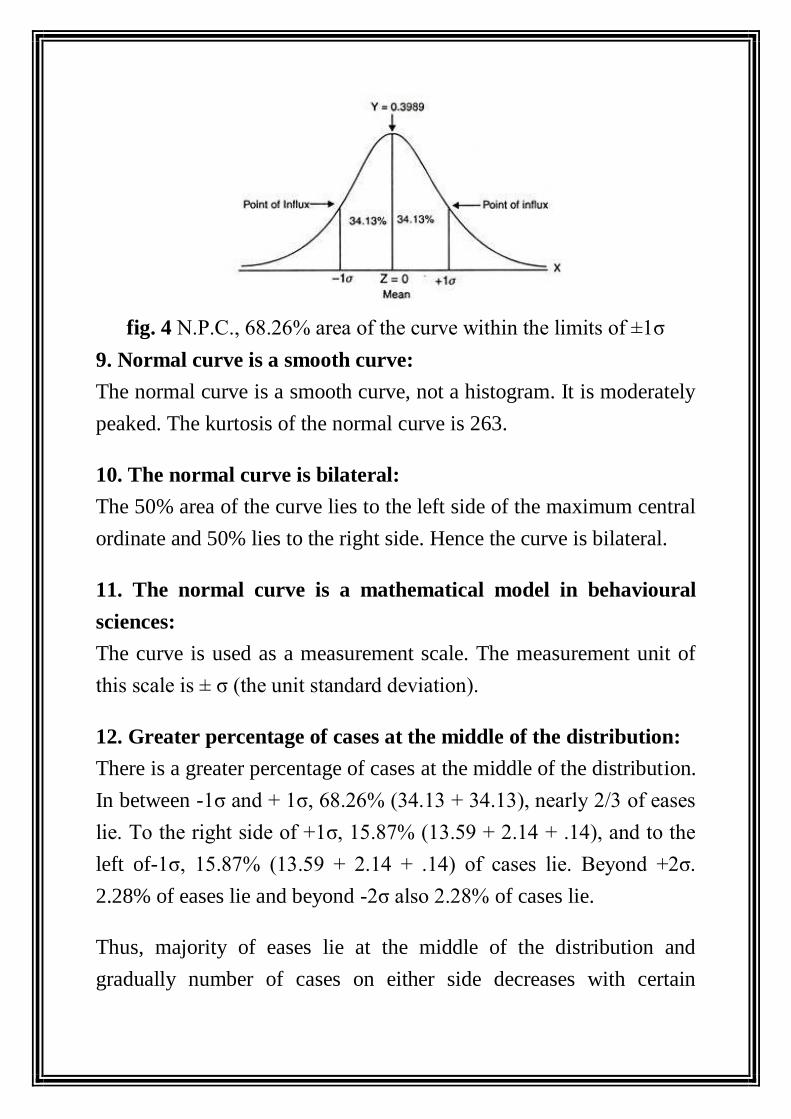
fig. 4 N.P.C., 68.26% area of the curve within the limits of ±1σ

9. Normal curve is a smooth curve:

The normal curve is a smooth curve, not a histogram. It is moderately

peaked. The kurtosis of the normal curve is 263.

10. The normal curve is bilateral:

The 50% area of the curve lies to the left side of the maximum central

ordinate and 50% lies to the right side. Hence the curve is bilateral.

11. The normal curve is a mathematical model in behavioural

sciences:

The curve is used as a measurement scale. The measurement unit of

this scale is ± σ (the unit standard deviation).

12. Greater percentage of cases at the middle of the distribution:

There is a greater percentage of cases at the middle of the distribution.

In between -1σ and + 1σ, 68.26% (34.13 + 34.13), nearly 2/3 of eases

lie. To the right side of +1σ, 15.87% (13.59 + 2.14 + .14), and to the

left of-1σ, 15.87% (13.59 + 2.14 + .14) of cases lie. Beyond +2σ.

2.28% of eases lie and beyond -2σ also 2.28% of cases lie.

Thus, majority of eases lie at the middle of the distribution and

gradually number of cases on either side decreases with certain

proportions. Percentage of cases between Mean and different a

distances can be read from the figure below:

fig. 5

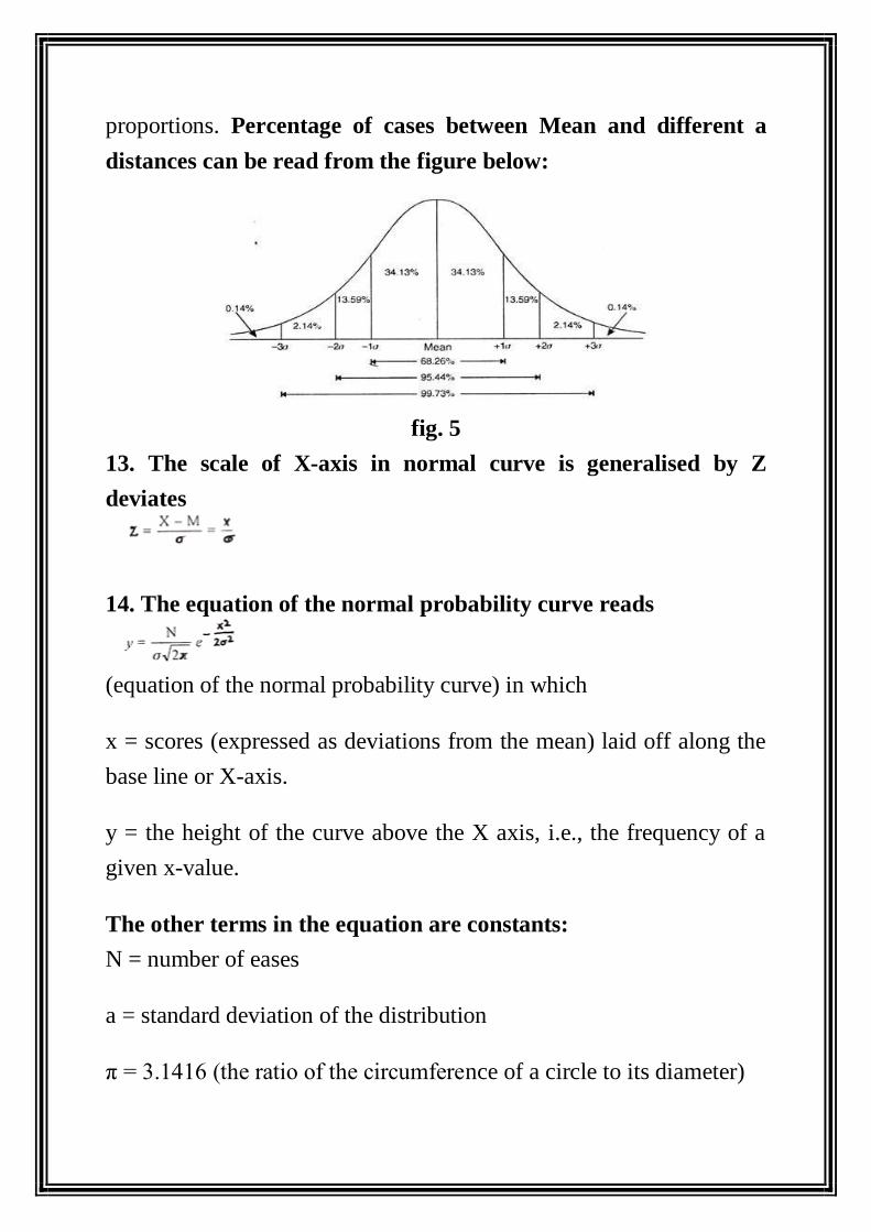
13. The scale of X-axis in normal curve is generalised by Z

deviates

14. The equation of the normal probability curve reads

(equation of the normal probability curve) in which

x = scores (expressed as deviations from the mean) laid off along the

base line or X-axis.

y = the height of the curve above the X axis, i.e., the frequency of a

given x-value.

The other terms in the equation are constants:

N = number of eases

a = standard deviation of the distribution

π = 3.1416 (the ratio of the circumference of a circle to its diameter)

e = 2.7183 (base of the Napierian system of logarithms).

15. The normal curve is based on elementary principles of

probability and the other name of the normal curve is the ‘normal

probability curve’.

Conclusion: -

Hence, we come to a result that NPC has various characteristics and

hence it has various uses and applications too. NPC is symmetrical,

unimodal, asymptotic to x-axis, bilateral and many more.

Reference: -

www.google.com

(B) QUES. TAKING SOME EXAMPLES

DESCRIBES APPLICATIONS OF NPC.

Laplace and Gauss (1777-1855), derived the NORMAL

PROBABLITITY CURVE independently, so the curve is also

known as Gaussian Curve in the honor of Guass.

NPC is the frequency polygon of any normal distribution. It is an

ideal symmetrical frequency curve and is supposed to be based on the

data of a population.

So, it is clear from the definitions and characteristics of NPC that

NPC is the “Graph of the probability density function of the

normal distribution is a continuous bell shaped curve,

symmetrical about the mean”.

Applications of Normal Probability Curve:

Some of the most important applications of normal probability

curve are as follows:

The principles of Normal Probability Curve are applied in the

behavioural sciences in many different areas.

1. NPC is used to determine the percentage of cases in a normal

distribution within given limits:

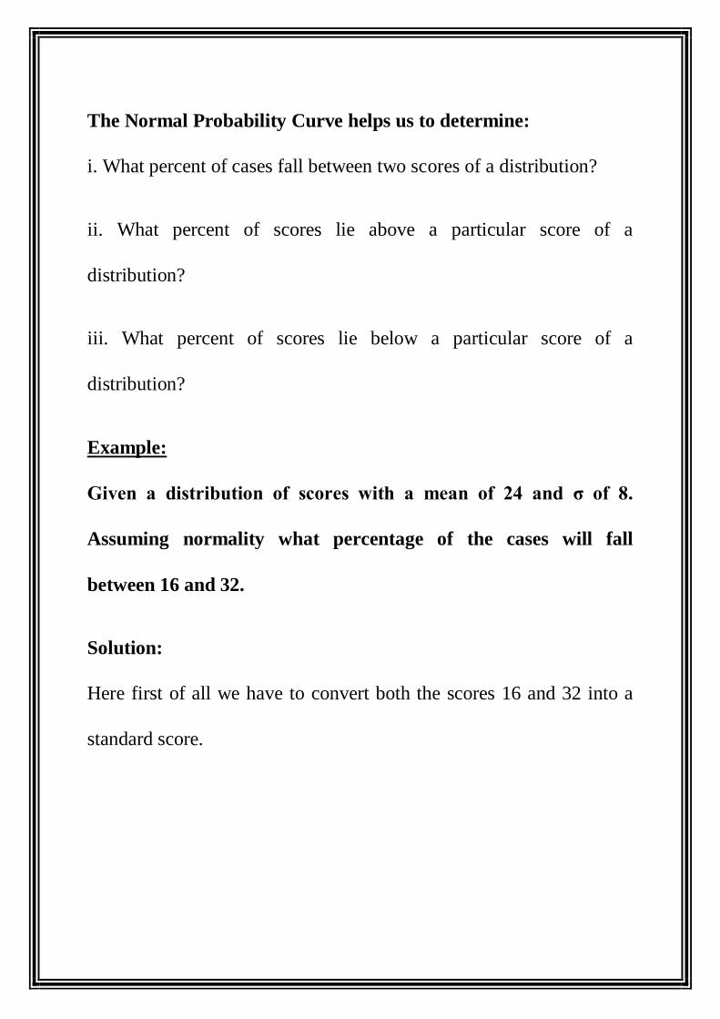
The Normal Probability Curve helps us to determine:

i. What percent of cases fall between two scores of a distribution?

ii. What percent of scores lie above a particular score of a

distribution?

iii. What percent of scores lie below a particular score of a

distribution?

Example:

Given a distribution of scores with a mean of 24 and σ of 8.

Assuming normality what percentage of the cases will fall

between 16 and 32.

Solution:

Here first of all we have to convert both the scores 16 and 32 into a

standard score.

Entering in to the Table-A, the table area under NPC, it is found that

34.13 cases fall between mean and – 1σ and 34.13 cases fall between

mean and + 1σ. So ± σ covers 68.26% of cases. So that 68.25% cases

will fall between 16 and 32.

Example:

Given a distribution of scores with a mean of 40 and σ of 8.

Assuming normality what percentage of cases will lie above and

below the score 36.

Solution:

First of all we have to convert the raw score 36 into standard score.

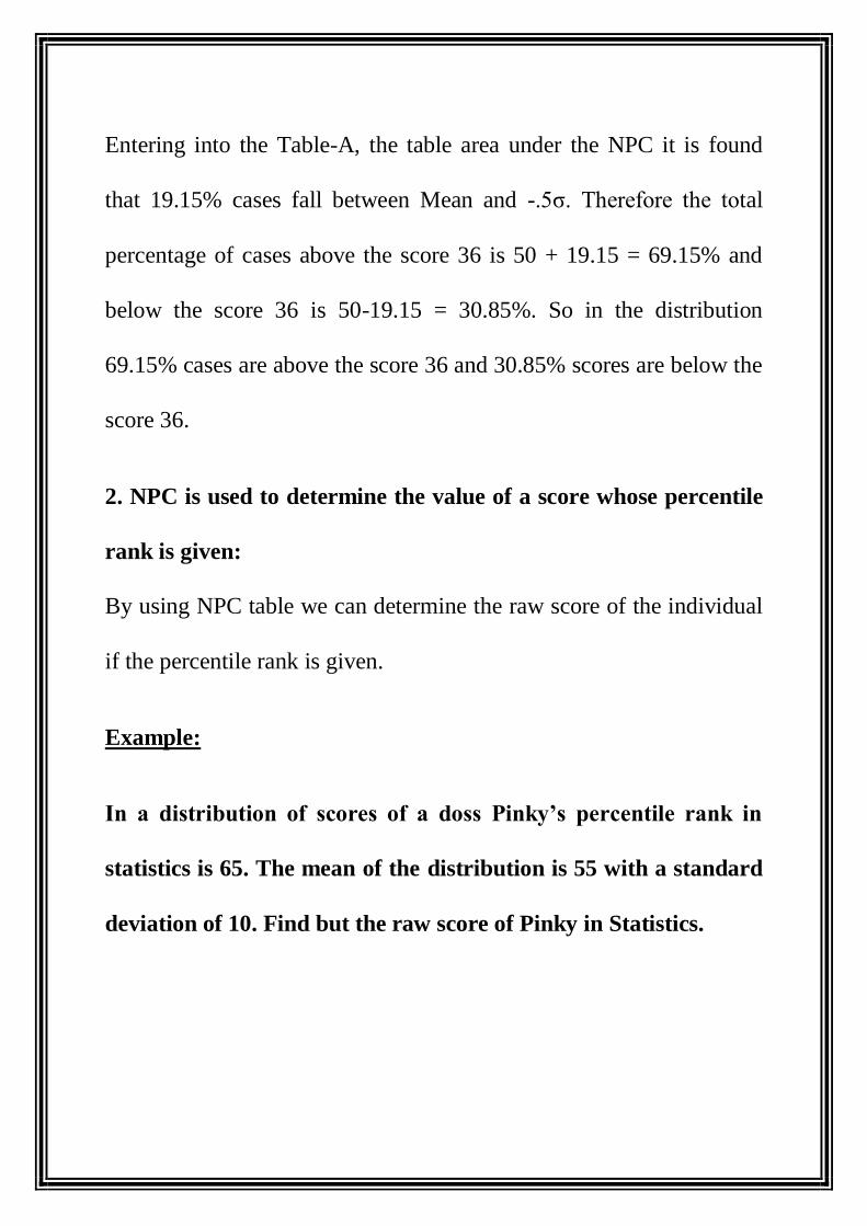
Entering into the Table-A, the table area under the NPC it is found

that 19.15% cases fall between Mean and -.5σ. Therefore the total

percentage of cases above the score 36 is 50 + 19.15 = 69.15% and

below the score 36 is 50-19.15 = 30.85%. So in the distribution

69.15% cases are above the score 36 and 30.85% scores are below the

score 36.

2. NPC is used to determine the value of a score whose percentile

rank is given:

By using NPC table we can determine the raw score of the individual

if the percentile rank is given.

Example:

In a distribution of scores of a doss Pinky’s percentile rank in

statistics is 65. The mean of the distribution is 55 with a standard

deviation of 10. Find but the raw score of Pinky in Statistics.

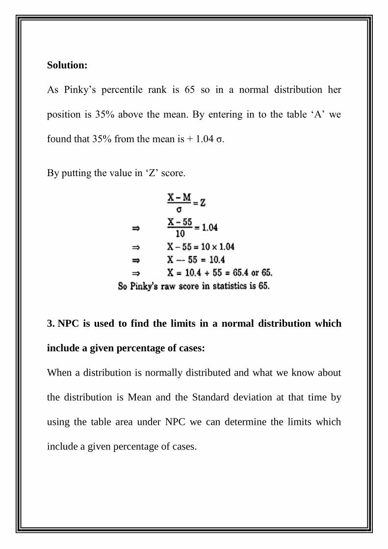
Solution:

As Pinky’s percentile rank is 65 so in a normal distribution her

position is 35% above the mean. By entering in to the table ‘A’ we

found that 35% from the mean is + 1.04 σ.

By putting the value in ‘Z’ score.

3. NPC is used to find the limits in a normal distribution which

include a given percentage of cases:

When a distribution is normally distributed and what we know about

the distribution is Mean and the Standard deviation at that time by

using the table area under NPC we can determine the limits which

include a given percentage of cases.

Example:

Given a distribution of scores with a mean of 20 and σ of 5. If we

assume normality what limits will include the middle 75% of

cases.

Solution:

In a normal distribution the middle 75% cases include 37.5% cases

above the mean and 37.5% cases below the mean. From the Table-A

we can say that 37.5% cases covers 1.15 σ units. Therefore the middle

75% cases lie between mean and ± 1.15 σ units.

So in this distribution middle 75% cases will include the limits 14.25

to 25.75.

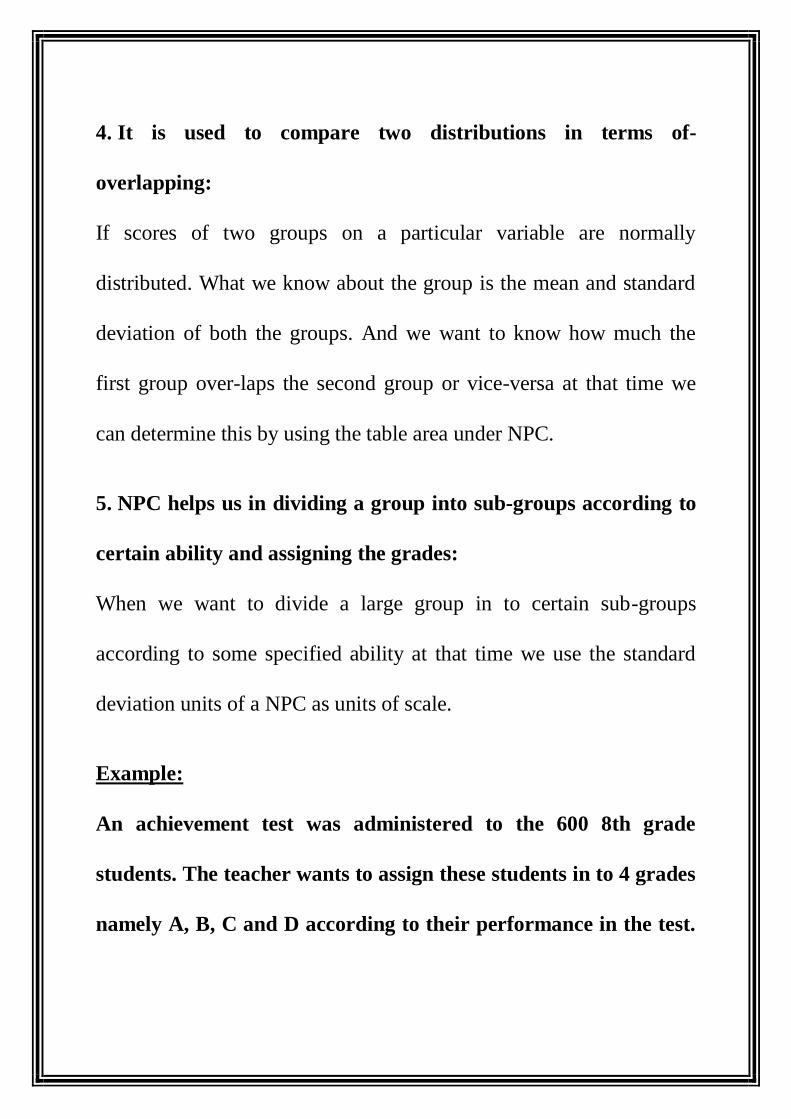
4. It is used to compare two distributions in terms of-

overlapping:

If scores of two groups on a particular variable are normally

distributed. What we know about the group is the mean and standard

deviation of both the groups. And we want to know how much the

first group over-laps the second group or vice-versa at that time we

can determine this by using the table area under NPC.

5. NPC helps us in dividing a group into sub-groups according to

certain ability and assigning the grades:

When we want to divide a large group in to certain sub-groups

according to some specified ability at that time we use the standard

deviation units of a NPC as units of scale.

Example:

An achievement test was administered to the 600 8th grade

students. The teacher wants to assign these students in to 4 grades

namely A, B, C and D according to their performance in the test.

Assuming the normality of the distribution of scores calculate the

number of students can be placed in each group.

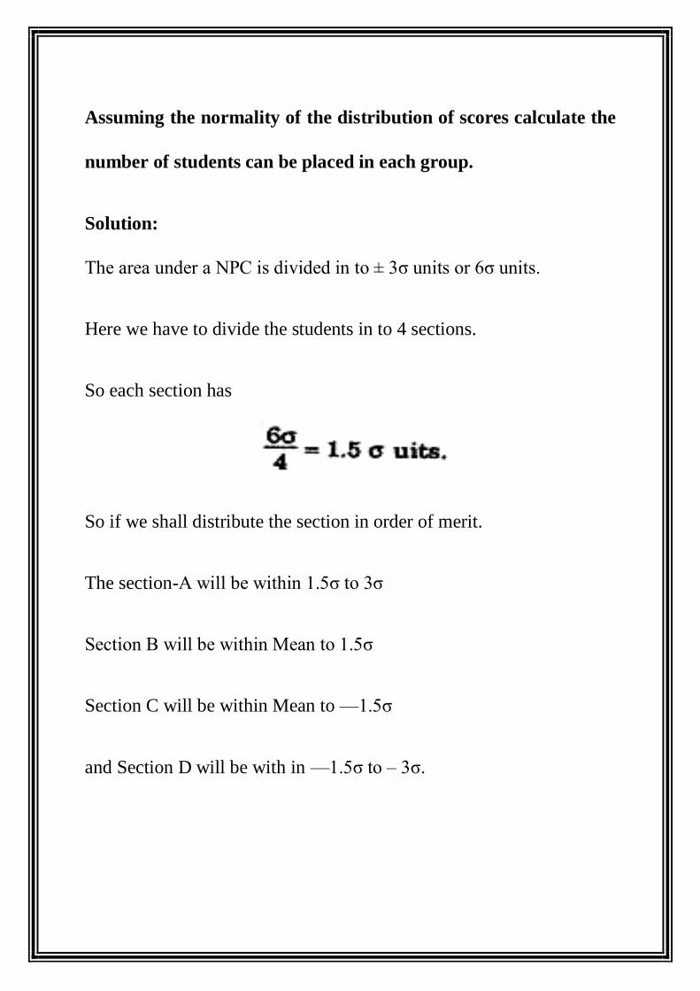
Solution:

The area under a NPC is divided in to ± 3σ units or 6σ units.

Here we have to divide the students in to 4 sections.

So each section has

So if we shall distribute the section in order of merit.

The section-A will be within 1.5σ to 3σ

Section B will be within Mean to 1.5σ

Section C will be within Mean to —1.5σ

and Section D will be with in —1.5σ to – 3σ.

6. NPC helps to determine the relative difficulty of test items or

problems:

When it is known that what percentage of students successfully

solved a problem we can determine the difficulty level of the item or

problem by using table area under NPC.

7. NPC is useful to normalize a frequency distribution:

In order to normalize a frequency distribution we use Normal

Probability Curve. For the process of standardizing a psychological

test this process is very much necessary.

8. To test the significance of observations of experiments we use

NPC:

In an experiment we test the relationship among variables whether

these are due to chance fluctuations or errors of sampling procedure

or it is real relationship. This is done with the help of table area under

NPC.

9. NPC is used to generalize about population from the sample:

We compute standard error of mean, standard error of standard

deviation and other statistics to generalize about the population from

which the sample are drawn. For this computation we use the table

area under NPC.

CONCLUSION: -

Hence, we come to a conclusion that NPC is used to determine the

percentage of cases in normal distribution within given limits. It is

also used to compare two distributions in terms of- overlapping. It

also helps us in dividing a group into sub-groups according to certain

ability and assigning the grades etc.

REFERENCE: -

www.google.com