Decline Curve Analysis for Sudanese Oilfield

Sudan University of Science and Technology

College of Petroleum Engineering and Technology

Department of Petroleum Engineering

Decline Curve Analysis for

Sudanese Oilfield

Case Study (South Al-Najma Oilfield)

تحليل منحنى الهبوط لحقل نفط سوداني

(17)مربع حالةدراسة

This dissertation is submitted as a partial requirement of

B.Tech. Degree (Honor) in Petroleum Engineering

Prepared by

1. Ahmad Ibrahim Mohamed

2. Ibrahim Mohamed Ibrahim

3. Moawia Mohamed A.Jalil

4. Omer Mohamed Elhaj

Supervisor:

Dr. Elradi Abass

October 2017

i

االستــــهالل

قال ربنا جل وعال :

وح من } وح قل الر ما أوتيتم و ب ي مر ر أ ويسألونك عن الر

ن العلم )85(قم رسراء األية {سورة ال إلا قليل م

صدق هللا العظيم

ii

شكر وتقدير

ي لسانا ايها الشعر للشكرأ عرن

وان تطق شكرا فال كنت من شعر

ي الذين ، يات الشكر والتقدير لمنارات العلم والمعرفة آ سىمأنزج

حتى وصلنا إىل هنا .. الثمي من وقتهم أعارونا

iii

تجريـــــد

ج اقبة إنتايعتبر النفط من أهم الصناعات التي تتحكم بالقتصاد العالمي ،لذلك من المهم مر

لدراسة النفط وتوقع النتاج في المستقبل ،ومن هنا أتت الحوجة إلى تطوير الكثير من البحوث

معدلت إنخفاض النتاج.

فط النانتاج معدلت نخفاضامنحيات األنخفاض هو تمثيل بياني يستخدم لتحليل تحليل

التنبؤ بأدائية المكمن في المستقبل.وكذلك والغاز للحقول النفطية

ون أن معدلت النتاج تنخفض كدالة في الزمن وذلك بالنسبة ألنخفاض ضغط المكمن ويك

المنتجة من المكمن ذاته. حجوم الموائع في تغيرالالسبب في ذلك عادة هو

لمكمن عبر تمثيل هذه البيانات بيانيا يمكن رسم منحنيات النخفاض التاريخي لدائية ا

أنهف، من الرسم الناتج المنحني اتجاه سلك نفسيسالمستقبلي األنخفاض لوبأفتراض أن معد

.وايضا حساب كمية الستخلص النهائي المتوقع مستقبليا يمكن التنبؤ باداء المكمن

نفطي والذي يقع في غرب ال South Al-Najma لحقل 17 في هذا البحث فأن مربع

تحليل لتم اخذه كمثال تطبيقي قد برميل في اليوم 3,860 وتقدر انتاجيته الكلية ب السودان

منحنيات األنخفاض في األنتاج .

سةدرالمنحنيات األنخفاض وذلك باستخدام وسائل مختلفة لقامت الدراسة بأجراء تحليل

باألضافة الي Oilfield Manager (OFM-Software)من أهمها برنامج ، هذا األنخفاض

اجريت المقارنة بين النتائج ، وقد Microsoft Excel Sheet (MS-Excel Sheet)برنامج

.المتحصل عليها بواسطة كل من الطريقتين

لنهائي لجهة التنبؤ بمستقبل األنتاج وكمية الستخلص ا جدا النتائج متقاربة تبين أن

.خلل العشر سنوات المقبلة المتوقع

iv

Abstract

Oil and gas is the key word for industrial revolutionary occur worldwide, as in

past and present the necessity of close monitoring for the oil and gas supply

production.

Decline curve analysis (DCA) is a graphical representation used for analyzing

declining production rates and predicting the future production performance of oil and

gas wells. The production rates declines as a function of time; reservoir pressure

drawdown, the change of the produced fluids volumes, are usually the cause. Fitting a

line through the performance history and assuming this same trend will continue in

future forms the basis of Decline curve analysis concept.

In this research block (17) of South Al-Najma oil field which located in western

Sudan, it’s with a total current productivity of (3, 68 0 bbl./day), the data collected

from the area has been used as an applicable for decline curve analysis study

The study conducts a decline curve analysis procedure, which have a variety of

supporting tools, the most common type of these tools are oilfield manager (OFM-

Software) and Micro-Soft Excel sheet (MS-Excel). A comparison study between

Micro-soft Excel sheet and OFM-Software results has been done.

A Comparison study the result show identical feature from the two procedures.

v

List of Content

I ......................................................................................................... االستــــهالل

II ...................................................................................................... شكر وتقدير

III ............................................................................................................ تجريـــــد

ABSTRACT ................................................................................................... IV

LIST OF CONTENT ......................................................................................... V

LIST OF TABLES ........................................................................................... VII

LIST OF FIGURES ........................................................................................ VIII

1. CHAPTER ONE ........................................................................................ 1

INTRODUCTION ............................................................................................ 1

INTRODUCTION: ................................................................................. 1

FIELD BACKGROUND:.......................................................................... 2

PROBLEM STATEMENT: ...................................................................... 3

RESEARCH OBJECTIVES: ...................................................................... 4

PROJECT LAY OUT: .............................................................................. 4

2. CHAPTER TWO ....................................................................................... 5

LITERATURE REVIEW AND THEORETICAL BACKGROUND ................................ 5

LITERATURE REVIEW: ......................................................................... 5

THEORETICAL BACKGROUND: ............................................................. 7

DECLINE TYPES: ...................................................................................... 8

2.2.1.1 Exponential Decline: ..................................................................... 8

2.2.1.2 Hyperbolic Decline: ....................................................................... 9

2.2.1.3 Harmonic Decline: ...................................................................... 10

FETKOVICH DECLINE TYPE CURVE: ............................................................ 13

3. CHAPTER THREE .................................................................................... 15

vi

THE METHODOLOGY .................................................................................... 15

METHODOLOGY BRIEF: ...................................................................... 15

DECLINE CURVE ANALYSIS TOOLS ...................................................... 15

MICROSOFT EXCEL SHEET: ...................................................................... 16

OIL FIELD MANAGER (OFM) SOFTWARE: .................................................. 16

OFM-SOFTWARE RULES: ....................................................................... 18

4. CHAPTER FOUR ..................................................................................... 19

RESULTS AND DISCUSSION .......................................................................... 19

DATA COLLECTION ............................................................................. 19

RESULTS AND DISCUSSION: ............................................................... 20

MICROSOFT EXCEL SHEET RESULTS: .......................................................... 20

4.2.1.1 South Al-Najma 01 (SA-01): ........................................................ 21

4.2.1.2 South Al-Najma 05 (SA-05): ........................................................ 22

4.2.1.3 South Al-Najma Field (SA-Entire Field): ...................................... 24

OFM SOFTWARE RESULTS: ..................................................................... 25

COMPARISON BETWEEN OFM-SOFTWARE AND MS EXCEL SHEET RESULTS: ...... 27

5. CHAPTER FIVE CONCLUSION AND RECOMMENDATIONS ..................... 31

CONCLUSION: .................................................................................... 31

RECOMMENDATIONS: ....................................................................... 31

REFERENCES: ............................................................................................... 32

vii

List of Tables

TABLE 1 FIELD AVERAGE PRODUCTION YEARLY .......................................................................... 3

TABLE 2 EXPONENTIAL EQUATIONS (B=0) ............................................................................... 9

TABLE 3 HYPERBOLIC EQUATIONS (0<B<1) ............................................................................ 10

TABLE 4 HARMONIC DECLINE EQUATIONS (B=1)................................................................... 11

TABLE 5 SA-1DAILY PRODUCTION DATA ................................................................................ 19

TABLE 6 MASTER DATA FOR ENTIRE FIELD .............................................................................. 20

TABLE 7 SA-1 PARAMETERS (EXCEL SHEET) ........................................................................... 21

TABLE 8 SA-01 FLOW RATE VS. TIME (FORECASTING) ............................................................ 21

TABLE 9 SA-5 PARAMETERS (EXCEL SHEET) ........................................................................... 23

TABLE 10 SA-05 FLOW RATE VS. TIME (FORECASTING) ........................................................... 23

TABLE 11 SA- FIELD PARAMETERS (EXCEL SHEET) ................................................................... 24

TABLE 12 SA-ENTIRE FIELD FLOW RATE VS. TIME (FORECASTING) ............................................. 24

TABLE 13 AS-1 PARAMETERS (OFM)................................................................................... 26

TABLE 14 SA-5 PARAMETERS (OFM) ................................................................................... 26

TABLE 15 ENTIRE FIELD PARAMETERS (OFM) ......................................................................... 27

TABLE 16 ENTIRE FIELD COMPARISON IN RESULTS BETWEEN OFM-SOFTWARE AND EXCEL SHEET ..... 28

TABLE 17 SA-1 COMPARISON IN RESULTS BETWEEN OFM-SOFTWARE AND EXCEL SHEET .............. 28

TABLE 18 TABLE SA-5 COMPARISON IN RESULTS BETWEEN OFM-SOFTWARE AND EXCEL SHEET ...... 28

TABLE 19 WELLS DECLINE RATE .......................................................................................... 29

viii

List of Figures

FIGURE 1 A THEORETICAL PRODUCTION CURVE, DESCRIBING THE VARIOUS STAGES OF MATURITY ........ 2

FIGURE 2 FIELD MAP ........................................................................................................... 3

FIGURE 3 DECLINE CURVE SHAPES FOR A SEMI LOG PLOT OF RATE VS. TIME ................................ 11

FIGURE 4 DECLINE CURVE SHAPES FOR A SEMI LOG PLOT OF RATE VS. TIME ................................ 12

FIGURE 5 DECLINE CURVE SHAPES FOR A CARTESIAN PLOT OF RATE VS. CUMULATIVE ................... 12

FIGURE 6 DECLINE CURVE SHAPES FOR A CARTESIAN PLOT OF RATE VS. CUMULATIVE ................... 13

FIGURE 7 FETKOVICH DECLINE TYPE CURVE ............................................................................ 14

FIGURE 8 OFM SOFTWARE INTERFACE .................................................................................. 17

FIGURE 9 OFM MASTER DATA BAS ..................................................................................... 17

FIGURE (10) OFM-SOFTWARE FLOW CHART FOR DATA ANALYSIS & RESULTING: .......................... 18

FIGURE 11 SA-01 FLOW RATE VS. TIME (HISTORY) ON SEMI-LOG ............................................. 21

FIGURE 12 SA-01 FLOW RATE VS. TIME (FORECASTING ON SEMI-LOG) ...................................... 22

FIGURE 13 - 4.6, SA-05 FLOW RATE VS. TIME (HISTORY ON SEMI-LOG) ................................... 22

FIGURE 14 SA-05 FLOW RATE VS. TIME (FORECASTING ON SEMI-LOG) ....................................... 23

FIGURE 15, SA-ENTIRE FIELD FLOW RATE VS. TIME (HISTORY ON SEMI-LOG) ............................... 24

FIGURE 16 , SA-ENTIRE FIELD FLOW RATE VS. TIME (FORECASTING ON SEMI-LOG) ........................ 25

FIGURE 17 , SA-1 FLOW RATE VS. TIME (SEMI-LOG) .............................................................. 25

FIGURE 18 , SA-5 FLOW RATE VS. TIME (SEMI-LOG) ............................................................. 26

FIGURE 19 SA-ENTIRE FIELD FLOW RATE VS. TIME (SEMI-LOG) ............................................... 27

1

1. Chapter One

Introduction

Introduction

Oil is a black gore that runs through the veins of the modern global energy

system. In some senses, oil can be seen as the black soul of our industrialized

mechanized society and the trademark of lifestyle, its combustion brings energy in

immense amounts and can drive a wide array of machines, tools and processes, oil can

also be broken down and used as a feedstock in a wide range of chemical processes,

providing variety of products advances from medicines to plastics.

The aim of this thesis is to investigate fundamental properties and behavior of

crude oil production and examine some model approaches for creating realistic

outlooks for the future.

The decline curve analysis is the most effective and important way for

controlling and monitoring the oil production with predicting the parameters that can

make huge effect to the oil production.

The basis of decline-curve analysis is to match past production performance

histories or trends (i.e., actual production rate/time data) with a "model." Assuming

that future production continues to follow the past trend, we can use these models to

estimate original oil and gas in place and to predict ultimate oil and gas reserves at

some future reservoir abandonment pressure or economic production rate, or we can

determine the remaining productive life of a well or the entire field, in addition we

can estimate the individual well flowing characteristics, such as formation

permeability and skin factor, with decline-type-curve analysis techniques , Decline-

curve methods, however, are applicable to individual well or the entire field.

From about 1975 to 2005, various methods have been developed for estimating

reserves and fields performance.

These methods range from the basic material balance equation to decline- curve

and type-curve analysis techniques.

1. There are two kinds of decline-curve analysis techniques, namely:

Classical curve fit of historical production data.

2

2. Type-curve matching technique.

Some graphical solutions use the both methods

Figure 1 A theoretical production curve, describing the various stages of maturity.

Source: Robelius (2007)

Field background

In this approach targeting a Sudanese oilfield at Block 17 (South AL-Najma)

whose owned by an operating company, the field consist of Early Production Facility

(EPF), 43 km Pipeline and (14 wells).

South AL-Najma field distance from Khartoum State about 900 Km (Western

Sudan – Kourdofan), it has been put into operation since December 2012 and up to

date, producing 3,860 BBLS of oil from (14) wells, plus two wells one in Sharif field

and the other in Abou-Jabra field, now four out of these(14) wells were shut down.

Early production facility (EPF) and pipeline commissioned on Dec.2012.

The EPF is designed to process incoming of 22.5 KBPD with 35% WC, and

outcome of 15 KBPD with maximum 0.5% WC.

3

Figure 2 field map

Problem statement

Currently decreasing in oil production has been observed at South AL-Najma

oilfield due to reservoir pressure drop, it has been observed that the drop in

production, being faster than expected, so it’s necessary to conduct a decline curve

analysis procedure to extrapolate the future production profile for this oilfield.

South AL-Najma Decline in production rates as follows:

Table 1 Field average production yearly

Year Production average (bbl./day)

2013 5350

2014 8000

2015 7800

2016 4800

2017 3860

4

Research objectives

The main objective of this study is to forecasting the behavior of the wells or the

entire reservoir in future at South Al-Najma oilfield based on production declining for

the historical data collected.

The specific objectives studied as the following:

1. To predict the oil production for the next (10) years.

2. To Estimate Expected Ultimate Recovery (EUR) based on the decline curve

analysis.

3. Compare the results that will be achieved from Microsoft Excel computation

and Oil field manager software (OFM).

Project Lay Out

Chapter One:

Include introduction, project background, problem statement and objectives.

Chapter Two:

Here find enclose, literature review and theoretical background.

Chapter Three:

Represent project methodology.

Chapter Four:

Contain results and discussion.

Chapter Five:

Consist of conclusion and recommendations.

5

2. Chapter Two

Literature Review and Theoretical Background

This chapter presents the literature study on decline curve analysis with various

theories which used to analyze the decline curves of an abandoned well or entire

oilfield.

Literature Review:

H.M Roeser in 1925 showed that by using (Trial and error method), we could

obtain same equally & reliable results of the method of least squares. He illustrated

his method (Trail & Error) with examples of both the exponential & hyperbolic types

of decline-curves.

R.H Johnson & A.L Bollens in 1927 They introduced a novel statistical method

called (Loss ratio method).

A curve to be investigated with this method usually shows, after proper

smoothing out, either a constant loss-ratio or constancy in the differences of

successive loss-ratio.

H.C Miller in 1942 Introduced the pressure drop cumulative relationship on a

log-log paper, showed how changes in reservoir performance can be detected by

abrupt (declining sharply) changes in the slope of such a curve.

J.J ARPS, MEMBER A.I.M.E., (May 1944), declares that During a period of

severe production declining, production-decline curves will significantly losing their

importance to estimate the reserves, because the production rates of all wells were

constant or almost constant.

To solve this problem following engineering methods were developed to

understand reservoir performance:

1. Electric-logs

2. Core analysis Data

3. Bottom-hole pressure behavior

4. Physical characteristics of reservoir fluids.

6

Production rate is the most available and logic characteristic which we can rely

on to find out a solution for both problems shown above and the method will be either

one of the following:

1. Plotting this Variable (Production rate vs. time )

2. Plotting (Production rate vs. cumulative production).

Arps (1945) proposed that the “curvature” in the production-rate-versus-time

curve can be expressed mathematically by a member of the hyperbolic family of

equations. Arps recognized the following three types of rate-decline behavior:

1. Exponential decline

2. Harmonic decline

3. Hyperbolic decline

Ramsay, (1968) has expressed that rate-time decline curve extrapolation is one

of the oldest and most often used tools of the petroleum engineer. The various

methods used always have been regarded as strictly empirical and generally not

scientific. Results obtained for a well or leases are subject to a wide range of alternate

interpretations, mostly as a function of the experience and objectives of the evaluator.

Recent efforts in the area of decline curve analysis have been directed toward a purely

computerized statistical approach, its basic objective being to arrive at a unique

"unbiased" interpretation.

Mikael hook, kjell Aleklett, 2008, The field subclasses to giant oil, smaller oil

field, natural gas liquid, condensate

Giant field decline 13% annually, other fields decline faster especially

condensate about 40% annually forecasting for this field is important because Norway

is a major oil exporter and the decline will affect all who are dependent on it is export

methodology depended on all oil most be analyzed separately.

Conclusion normally will have dramatically reduced export volume of oil by

2030.

A.J. Clark, (2011) proposed a new empirical model for production forecasting in

extremely low permeability oil and gas reservoirs based on logistic growth models.

The new model incorporates known physical volumetric quantities of oil and gas into

the forecast to constrain the reserve estimate to a reasonable quantity.

7

The new model is easy to use, and it is very capable of trending existing

production data and providing reasonable forecasts of future production. The logistic

growth model does not extrapolate to non-physical values.

Khulud M. Rahuman, H. Mohamed, N. Hissein, and S. Giuma (April 2013)

Decline curve analysis is a technique can be applied to a single well, and total

reservoir.

Decline analysis routinely used by engineers to estimate initial hydrocarbon in

place, hydrocarbon reserves at some abandonment conditions, and forecasting future

production rate. The remaining reserve depends on the production points that selected

to represent the real well behavior.

Comparison between the hand calculation and decline curve analysis (DCA)

program give result nearly similar to each other by the end of the forecasting period.

Theoretical Background

Decline curve analysis is a technique can be applied to a single well, or entire

reservoir. Routinely used by engineers to estimate initial hydrocarbon in place,

hydrocarbon reserves at some abandonment conditions, and forecasting future

production rate.

The remaining reserve depends on the production points that selected to

represent the real behavior of the well, the way of dealing with the production data,

and the human errors that might happen during the life of the field.

Decline curve analysis is the most currently method used for reserve estimation

when historic production data are available and sufficient.

Decline curves were commonly used to represent or extrapolate the production

data are members of a hyperbolic family, the method of extrapolating a “trend” for the

purpose of estimating future performance must satisfy the condition that the factors

that caused changes in past performance, for example, decline in the flow rate, will

operate in the same way in the future. These decline curves are characterized by three

factors:

1. Initial production rate or the rate at some particular time.

2. Curvature of the decline.

3. Rate of decline.

8

Decline Types

Based on what has been covered so far, the engineer performing a decline curve

analysis (DCA) required being aware of the following:

1. The most representative period in history that will also represent future.

2. The decline trend during that period.

3. The start point (rate) of forecast.

4. The constraints under which the forecast needs to be made.

However one more factor, also extremely important at this stage is to determine

type of decline. Since the signature of shape may not be apparent on a log production

rate (q) vs. time (most used plot), literature provides many ways was to look at the

same data, combine this information with other knowledge about the fields before

making the conclusions.

Depending on the value of the decline exponent (b), the decline exponent has

three different types (Arps -1945):

2.2.1.1 Exponential Decline

In the exponential decline, the well’s production data plots as a straight line on a

semi log paper. The equation of the straight line on the semi log paper is given by

(b=0):

𝑞 = 𝑞𝑖𝑒−𝐷𝑖𝑡 …………………………… Eq. (2.1)

Where: q = Well’s production rate at time t, (STB/day)

𝑞𝑖 = Well’s initial production rate, (STB/day)

𝐷𝑖 = Initial nominal exponential decline rate, t=0, (𝑑𝑎𝑦−1)

b = Decline exponent

t = time (day)

9

Table 2 Exponential Equations (b=0)

Description Equation

Production rate 𝑞 = 𝑞𝑖𝑒−𝐷𝑖𝑡

Cumulative Oil Production 𝑁𝑃 =𝑞𝑖 − 𝑞

𝐷

Nominal Decline Rate 𝐷 = −𝑙𝑛 (1 − 𝐷𝑒)

𝐷𝑒 =𝑞𝑖 − 𝑞

𝑞𝑖

Effective Decline Rate 𝐷𝑒 = 1 − 𝑒−𝐷

Life 𝑡 =

𝑙𝑛 (𝑞𝑖/𝑞)

𝐷

2.2.1.2 Hyperbolic Decline

Alternatively, if the well’s production data plotted on a semi-log paper concaves

upward, and then it is modeled with a hyperbolic decline. The equation of the

hyperbolic decline is given by (0<b<1):

𝑞 = 𝑞𝑖(1 + 𝑏𝐷𝑖𝑡)−1

𝑏 ……………………..Eq. (2.2)





t = time (day)

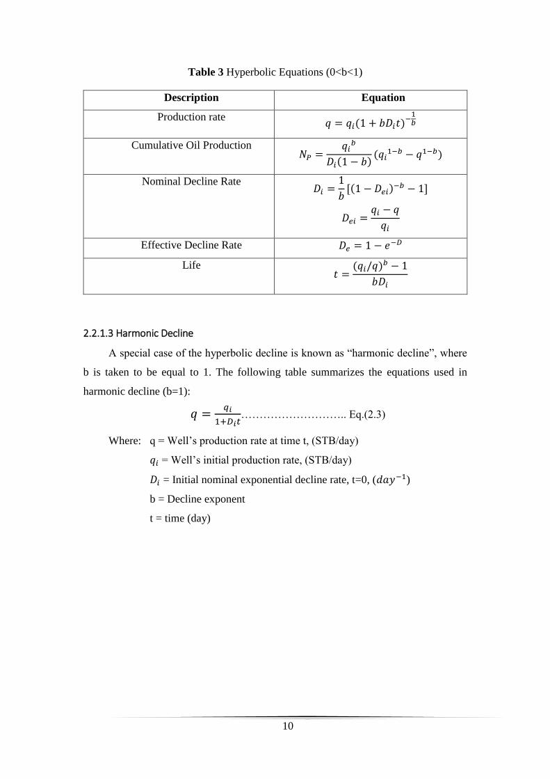
10

Table 3 Hyperbolic Equations (0<b<1)


Production rate 𝑞 = 𝑞𝑖(1 + 𝑏𝐷𝑖𝑡)−

1𝑏

Cumulative Oil Production 𝑁𝑃 =

𝑞𝑖𝑏

𝐷𝑖(1 − 𝑏)(𝑞𝑖

1−𝑏 − 𝑞1−𝑏)

Nominal Decline Rate 𝐷𝑖 =

1

𝑏 [(1 − 𝐷𝑒𝑖)

−𝑏 − 1]

𝐷𝑒𝑖 =𝑞𝑖 − 𝑞

𝑞𝑖

Effective Decline Rate 𝐷𝑒 = 1 − 𝑒−𝐷

Life 𝑡 =

(𝑞𝑖/𝑞)𝑏 − 1

𝑏𝐷𝑖

2.2.1.3 Harmonic Decline

A special case of the hyperbolic decline is known as “harmonic decline”, where

b is taken to be equal to 1. The following table summarizes the equations used in

harmonic decline (b=1):

𝑞 =𝑞𝑖

1+𝐷𝑖𝑡……………………….. Eq.(2.3)





t = time (day)

11

Table 4 Harmonic Decline Equations (b=1)


Production rate 𝑞 =𝑞𝑖

1 + 𝐷𝑖𝑡

Cumulative Oil Production 𝑁𝑃 =𝑞𝑖

𝐷𝑖ln (

𝑞𝑖

𝑞)

Nominal Decline Rate 𝐷𝑖 =

𝐷𝑒𝑖

1 − 𝐷𝑒𝑖

Effective Decline Rate 𝐷𝑒𝑖 =𝑞𝑖 − 𝑞

𝑞𝑖

Life 𝑡 =

(𝑞𝑖/𝑞) − 1

𝐷𝑖

The three decline curves have a different shape on Cartesian and semi-log

graphs of oil & gas production rate vs. time and oil & gas production rate vs.

cumulative gas production. Consequently, these curve shapes can help identify the

type of decline for a well and, if the trend is linear, extrapolate the trend graphically or

mathematically to some future point

Figure 3 Decline Curve Shapes for a Semi log plot of Rate VS. Time [john lee 1996]

12

Figure 4 Decline Curve Shapes for a Semi log plot of Rate VS. Time [john lee 1996]

Figure 5 Decline Curve Shapes for a Cartesian plot of Rate VS. Cumulative [john lee

1996]

13

Figure 6 Decline Curve Shapes for a Cartesian plot of Rate VS. Cumulative [John

lee 1996]

Fetkovich Decline Type Curve

The Fetkovich decline type curves are based on analytical solutions to the flow

equations for production at constant bottom hole pressure (BHP) from a well centered

in a circular reservoir or drainage area with no-flow boundaries. Although these type

curves were developed for a homogeneous-acting reservoir, they can be used for

analyzing long-term gas-production data from hydraulically fractured wells during the

pseudo radial flow period and once the outer reservoir boundaries affect the pressure

response. Fig. (7) is an example of the Fetkovich decline type curves for both

rate/time and cumulative production/time analyses.

14

Figure 7 Fetkovich Decline Type Curve

15

3. Chapter Three

The Methodology

Methodology Brief

Selecting an appropriate methodology is most the important process for accurate

forecasting the future production, as a planning to take the right decision should be

based on the recoverable percentage of the original hydrocarbon in place, as well as

the residual amount of this oil when the economic limit is reached before the need for

any secondary recovery mechanism is involved, for the case of a naturally producing

reservoir-well relationship.

Decline curve analysis (DCA) is a method used for the prediction of future

hydrocarbon production by analyzing past production.

Forecasting crude oil production can be done in many different ways, but in

order to provide realistic outlooks, one must be mindful of the physical laws that

affect extraction of hydrocarbons from a reservoir.

Decline curve analysis is a long established tool for developing future outlooks

for oil production from an individual well or an entire oilfield.

Extrapolation of production history has long been considered the most accurate

and defendable method of estimating the remaining recoverable reserve from a well

and, the entire reservoir.

Using decline curve analysis gives a better tool for describing future oil

production on a field-by-field level. Reliable and reasonable forecasts are essential for

planning and necessary in order to understand likely future world oil production.

Decline curve analysis tools

In this research two methods of decline curve analysis techniques have been

used, which include the following:

1. Microsoft Excel Sheet

2. Oil Field Manager (OFM Software)

16

Microsoft Excel Sheet

Using Microsoft Excel as per the following steps bellow: Calculating the decline

rate (D) from the equation given by Arps (1945)

𝐷 =1 ∗ dq

q ∗ dt… … … … … … … … … 𝐸𝑞(3.1)

1. Using daily production data to plot, oil flow rate versus time on a Semi-

log graph paper.

2. Depending on the curve shape which result from above plotting, decline

curve type will be identified as one of the following:

i. Exponential decline

ii. Harmonic Decline

iii. Hyperbolic Decline

3. Determining the Expected Ultimate Recovery (EUR) using:

EUR = historical oil cumulative + forecasting oil cumulative

Forecasting oil cumulative =𝑞𝑖

𝐷𝑖−

𝑞

𝐷𝑖 ……… Eq.(3.2)

Where: q = Production rate at the end of forecasting period, (bbl./day)

𝑞𝑖 = Initial Prod.Rate at the beginning of forecasting, (bbl./day)


Oil Field Manager (OFM) Software

For oilfield manager (OFM software), well and reservoir analysis software,

offers advanced production surveillance views and powerful production forecasting

tools to manage and improve oil and gas fields performance throughout the entire life

cycle of the field .

OFM software allows view, relate, and analyze reservoir and production data

with comprehensive workflow tools, such as interactive base maps with production

trends, bubble plots, diagnostic plots, decline curve analysis, and type curve analysis.

Recent architectural changes and usability improvements further enable organization

to be more productive.

The OFM application provides a privilege access to the data quickly, wherever

it may be located spreadsheets, databases, or other repositories. It also acts as a single

point of analysis for reservoir and production engineers to collaborate and manage

more wells in less time.

17

The multiple visualization canvases (charts, reports, and maps) and fast filtering

data fed to enable improvement for field performance by promptly identifying the

well or wells that offer an opportunity to increase production.

Figure 8 OFM Software Interface

Figure 9 OFM Master Data Bas

18

Figure (10) OFM-Software flow chart for Data Analysis & Resulting:

OFM-Software Rules

OFM-Software Forecasting module consists of four major categories

(techniques);

- Empirical (using Arps equations)

- Fetkovich

- Locke & Sawyer

- Analytical Transient solutions

Data•Master data

•Daily production data

Process •Forecasting

•Matching

Results •Graphs

•Maps

•Curves

•Tables

19

-

4. CHAPTER FOUR

Results and Discussion

Data collection

Data shown below is obtained from a field master data & daily production data:

Table 5 SA-1daily production data

Well Date THP CHP FLP FLT Choke size Pi Ti Fluid Oil

SA_1 22-Dec-12 200 100 500 53.9 12.8 1709 80 1589 1589

SA_1 23-Dec-12 200 100 500 53.8 12.8 1727 81 1589 1589

SA_1 24-Dec-12 200 100 500 53.8 12.8 1861 81 1521 1521

SA_1 25-Dec-12 230 120 490 46 10 1876 81 1343 1343

SA_1 26-Dec-12 230 120 490 46 10 1760 81 1265 1265

SA_1 27-Dec-12 250 140 495 47 10 1828 81 1265 1265

SA_1 28-Dec-12 220 100 495 50 11.5 1832 81 1406 1406

SA_1 29-Dec-12 250 120 495 49 10 1827 80.5 1462 1462

SA_1 30-Dec-12 250 120 495 48 10 1821 80 1456 1456

SA_1 31-Dec-12 250 120 495 47 10 1819 80 1413 1413

SA_1 01-Jan-13 250 120 495 47 10 1814 80 1341 1341

SA_1 02-Jan-13 245 120 495 49 10 1811 80 1331 1331

SA_1 03-Jan-13 245 120 495 49 10 1810 80 1325 1325

SA_1 04-Jan-13 245 120 495 49 10 1810 80 1343 1343

SA_1 05-Jan-13 245 120 495 49 10 1810 80 1307 1307

SA_1 06-Jan-13 245 100 490 49 10 1810 80 1315 1315

SA_1 07-Jan-13 245 100 495 48 10 1810 80 1272 1272

SA_1 08-Jan-13 250 105 500 49 10 1810 80 1322 1322

SA_1 09-Jan-13 250 105 500 49 10 1810 80 1364 1364

SA_1 10-Jan-13 240 95 490 48 10 1810 80 1352 1352

SA_1 11-Jan-13 245 100 495 48 10 1810 80 1341 1341

SA_1 12-Jan-13 240 100 500 48 10 1810 80 1359 1359

20

Table 6 Master data for entire field

Wells Completion

Type OGM name

Elevation Total depth

Formation Upper

perforation Lower

perforation

SA_1 B OGM_0 489.17 1900 Bentiu 1746 1758

SA_11 B OGM_1 489.17 2355 Bentiu 1806.63 1820.34

SA_12 B OGM_1 489.17 2592 Bentiu 1820.7 1823.3

SA_2 AG5 OGM_0 489.17 3607 AG 3240 3243

SA_3 Z OGM_0 476.16 1739 Zarga 1588 1600

SA_5 B OGM_0 489.17 2100 Bentiu 1755.5 1785

SA_6 B OGM_0 489.17 2114 Bentiu 1815 1825

SA_7A AG2 OGM_0 489.17 3097 AG 2748 2755

SA_7B B OGM_0 489.17 3097 Bentiu 1837.5 1844

SA_9 B OGM_1 489.17 2120 Bentiu 1782.5 1792.5

SA_15 B OGM_2 489.17 2000 Bentiu 1859 1932.5

SA_4 Basement OGM_0 489.17 1870 Basement NA NA

SA_8 AG OGM_0 540 3071 AG NA NA

SA_21 AG OGM_0 489.17 3017 AG 1879 1915

SA_13 AG OGM_0 489.17 3155 AG NA NA

SA_14 AG OGM_0 489.17 1741 AG 1573 1650

Results and Discussion

In this study two methods of decline curve analysis techniques have been used,

which include the following:

Microsoft Excel Sheet Results

1. Graphs shown hereinafter are results of plotting the field collected data using

MS-Excel sheet.

2. Tables shown here results from calculations of decline rate using formulas.

3. For best of analyzing& understanding the Production severe declining, South

Al-Najma wells (1 and 5) and in addition to entire field daily production and

accumulative Production data has been chosen as an applicable example to run

the calculations in this approach.

21

4.2.1.1 South Al-Najma 01 (SA-01)

Figure 11 SA-01 Flow Rate vs. time (History) on Semi-log

Table 7 SA-1 Parameters (Excel sheet)

Decline Exponent (b)

Prod. Rate(qi) (bbl/d)

Decline Rate (D) (1/day)

Forecast. Starting(Ti)

0 1055 0.002756 1/4/2017

For table (8), production rates at date from (01/31/2017) until (12/31/2027) has

been calculated using Eq. (2.1)

Table 8 SA-01 Flow Rate vs. time (Forecasting)

Date Production rate (bbl/d)

01/04/2017 1055

01/31/2017 1052.419

08/31/2021 904.2044

10/31/2025 787.5798

12/31/2027 733.0379

1

10

100

1000

10000

01-Apr-12 14-Aug-13 27-Dec-14 10-May-16 22-Sep-17

Rat

e b

bl/

d

Time (day)

Oil

Linear (Oil)

22

Figure 12 SA-01 Flow Rate vs. time (Forecasting on Semi-log)

3.2.1.2 South Al-Najma 05 (SA-05)

Figure 13 - 4.6, SA-05 Flow Rate vs. Time (History on Semi-log)

1

10

100

1000

10000

12/27/2014 9/22/2017 6/18/2020 3/15/2023 12/9/2025 9/4/2028

Rate vs Time

1

10

100

1000

10000

01-Apr-1214-Aug-1327-Dec-1410-May-1622-Sep-17

Rat

e b

bl/

d

Time (day)

oil rate

Linear (oil rate)

23

Table 9 SA-5 Parameters (Excel sheet)





0 1166

0.013618 1/4/2017



Table 10 SA-05 Flow Rate vs. Time (forecasting)

Date Rate

1/4/2017 1166

1/31/2017 1151.989

8/31/2021 551.3

10/31/2025 275.5427

12/31/2027 193.3664

Figure 14 SA-05 Flow rate vs. Time (forecasting on Semi-log)

1

10

100

1000

10000

12/27/20145/10/20169/22/20172/4/20196/18/202010/31/20213/15/20237/27/202412/9/20254/23/20279/4/2028

Rate vs Time

24

4.2.1.3 South Al-Najma Field (SA-Entire Field)

Figure 15 SA-Entire Field Flow Rate vs. Time (history on Semi-log)

Table 11 SA- Field Parameters (Excel sheet)





0 4159.42

0.00384 1/4/2017



Table 12 SA-Entire Field Flow Rate vs. Time (forecasting)

Date Rate

1/4/2017 4159.42

1/31/2017 4145.26765

8/31/2021 3356.10133

10/31/2025 2769.46386

12/31/2027 2506.29019

1

10

100

1000

10000

100000

4/1/2012 8/14/2013 12/27/2014 5/10/2016 9/22/2017

Rat

e b

bl/

d

Time (day)

oil rate

25

Figure 16 SA-Entire Field Flow Rate vs. Time (forecasting on semi-log)

OFM Software Results

1. Graphs shown hereinafter are results of plotting the field collected data

using OFM-Software.

2. Tables shown here outcomes from OFM-Software output results.

3. South Al-Najma (1&5) along with entire field daily production and

accumulative Production data has been used as an example.

Figure 17 SA-1 Flow Rate vs. Time (Semi-log)

1

10

100

1000

10000

12/27/2014 9/22/2017 6/18/2020 3/15/2023 12/9/2025 9/4/2028

Rate vs Time

26

Table 13 AS-1 Parameters (OFM)

Figure 18 SA-5 Flow Rate vs. Time (Semi-log)

Table 14 SA-5 parameters (OFM)

b Di (M.n.) qi (bbl/d) ti Te qe (bbl/d) Res. (Mbbl)

0.00 0.003370 1055 1/4/2017 12/31/2027 676.472 3418.13

b Di (M.n.) qi (bbl/d) ti Te qe (bbl/d) Res. (Mbbl)

0.00 0.014021 1166 1/4/2017 12/31/2027 183.592 2132.62

27

Figure 19 SA-Entire Field Flow Rate vs. Time (Semi-log)

Table 15 Entire Field parameters (OFM)

Comparison between OFM-Software and MS Excel sheet

results

After using data collected from the field and hence applied the decline curve

analysis methods here enclose is the concise of comparison between both tools which

been used in this research as it appears at the following schedules:

b Di (M.n.) qi (bbl/d) (ti) (te) (qe) (bbl/d) Res. (M.bbl) 0.00 0.004162 4159.42 1/4/2017 12/31/2027 2402.54 12845.7

28

Table 16 entire field Comparison in results between OFM-software and Excel Sheet

Parameters OFM Excel Sheet

Di 0.004162 0.00384

qi(bbl/d) 4159.42 4159.42

Historical

cumulative(Mbbl.)

9350.43 9350.43

Final rate at 2017 (bbl./d) 2402.54 2506.29

EUR (Mbbl.) 22196.1 22446.326

Table 17 SA-1 Comparison in results between OFM-software and Excel Sheet


Di 0.00337 0.00276

qi(bbl/d) 1055 1055

Historical

cumulative(Mbbl)

1839.5 1839.5

Final rate at 2017 (bbl/d) 676.472 733.0379

EUR (Mbbl.) 5257.63 5388.082

Table 18 Table SA-5 Comparison in results between OFM-software and Excel Sheet


Di 0.01402 0.01362

qi(bbl/d) 1166 1166

Historical

cumulative(M.bbl)

3154.82 3154.82

Final rate at 2017 (bbl/d) 183.592 193.366

EUR (M.bbl.) 5287.44 5327.18

Comparison shown above, indicate that results obtained from OFM-Software

and Excel sheet were likely similar to each other, except for values (Final rate, EUR)

which being calculated using Excel sheet were little bit higher than OFM–Software

29

results, this due to the fact that the decline rate calculated by Excel sheet is slightly

less than OFM.

Meaning to say that when using OFM-Software accurate result is obtained,

because choosing the decline rate is more accurate and less error than using Excel

sheet, also the best straight line on OFM-software using filtered data, but in Excel

sheet just the real data without filtration is being used.

By the other hand using Excel sheet will give somehow good result can be used

for the future forecasting for individual well or entire field.

Table 19 Wells Decline rate

Well Name Di

SA-7 A 0.4278

SA-17 0.1609

SA11 0.1303

SA-23 0.1083

SA-C-1 0.0725

SA-7B 0.0696

SA-21 0.0066

SA-12 0.0641

SA-9 0.0594

SA-5 0.0140

SA-15 0.0506

SA-18 0.0058

SA-1 0.00337

SA-6 0.00335

Table (19) shows the decline rate for individual well, sorted in descending

order for a purpose of comparison.

Out of this a conclusion can be made that wells with a high rate of decline will

have a greater and faster expected declining in productivity than those with a low rate

of decline, therefore, wells with a low rate of decline expected to maintain the total

productivity of the entire field for a longer period of time.

30

Note that when the decline rate (D) is high means the production rate will

decrease faster than expected, so the experience revealed that the decline in

production affected by many factors like the artificial life applied and the production

adjustment, such as choke size and pumps frequency.

31

5. Chapter Five

Conclusion and Recommendations

Conclusion

The study uses the historical production data that collected from day one of

the starting of production, until April 2017.

Using OFM software and Microsoft excel for the decline curve analysis allow

a verification result of prediction of production performance for field or

individual well.

The study uses the historical deterioration in production; the exponential

decline method has been used to gain best results.

The comparison between OFM and Micro-Soft Excel both are provide similar

results.

The forecasting results are achieved considering the next 10 years.

The Expected Ultimate Recovery (EUR), calculated by the end of Year 2027

for entire field.

The benefit from decline curve analysis is to figure out the future production,

that’s to optimize and develop the field before it reaches the abandonment

point.

Recommendations

1. In case of using OFM software it’s preferable to be applied for the naturally

produced well, to achieve best and accurate results of decline curve analysis

technique, the reservoir must be put into production of natural energy drive

without any intervention by further recovery methods.

2. When there are some wells producing naturally the right discussion is to keep

them run naturally instead of installing down hole pumps.

3. This study focus only on the future perdition of the field without considering

the economic side, so its recommended that incase a new study made,

economic can be taken into consideration.

4. Its recommended to conduct an EOR process in association with decline curve

analysis to give more hands so such problem.

32

References

1. Agarwal, R. G., Gardner, D. C., Kleinsteiber, S. W., and Fussell, D. D.,

September 1998, “Analyzing Well Production Data Using Combined Type

Curve and Decline Curve Analysis Concepts,” SPE 49222, SPE Annual

Technical, Conference and Exhibition, New Orleans, LA.

2. Ahmed, Tared H., 2000, Reservoir engineering handbook, by Gulf Publishing

Company, Houston, Texas.

3. A.J. Clark, (2011), Production Forecasting with Logistic Growth Models,

SPE -144790-MS , L.W. Lake, T.W. Patzek, University of Texas at Austin.

4. Anash, J., Blasingame, T. A., and Knowles, R. S., December 2000, “A Semi-

Analytic (p/z) Rate-Time Relation for the Analysis and Prediction of Gas Well

Performance”, SPE Reservoir Eval. & Eng. 3(6), USA.

5. Arps, J. J., 1945 , “Analysis of Decline Curves,” Trans. AIME.,. Volume160,

page 228–231.

6. Begland, T., and Whitehead, W., August 1989, “Depletion Performance of

Volumetric High-Pressured Gas Reservoirs,” SPE Reservoir Engineering, , pp.

279–282, USA.

7. Carter, R, Oct 1985, “Type Curves for Finite Radial and Linear Flow System”,

SPE J 719–728.

8. Chen, H.-Y., and Teufel, L. W., April 2002, “Estimating Gas Decline

Exponent before Decline Curve Analysis, ” SPE 75693, SPE Gas Technology

Symposium, Calgary, Alberta, Canada.

9. John Lee, Well testing handbook, 1996, by the Society of Petroleum

Engineers, United States of America.

10. Khulud M. Rahuma, H. Mohamed, N. Hissein, and S. Giuma (April 2013)

Prediction of Reservoir Performance Applying Decline Curve Analysis

International Journal of Chemical Engineering and Applications, Vol. 4, No.

11. Mikael Hook, Kjell Aleklett, November 11, 2008, Decline rate study of

Norwegian oil production, Uppsala University, Sweden.

12. Mikael Hook, May 2009, Depletion and decline curve analysis in crude oil

production, Uppsala University, Sweden.

Decline Curve Analysis for Sudanese Oilfield

Documents

Transcript of Decline Curve Analysis for Sudanese Oilfield