Abstract

The Curve Indicator Random Field

Jonas August

2001

Can the organization of local image measurements into curves be directly related

to natural image structure? By viewing curve enhancement as a statistical estimation

problem, we suggest that it can. In particular, the classical Gestalt perceptual

organization cues of proximity and good continuation—the basis of many current

curve enhancement systems—can be statistically measured in images. As a prior

for our estimation approach we introduce the curve indicator random field (cirf).

Technically, this random field is a superposition of local times of Markov processes

that model the individual curves; intuitively, it is an idealized artist’s sketch, where

the value of the field is the amount of ink deposited by the artist’s pen. The explicit

formulation of the cirf allows the calculation of tractable formulas for its cumulants

and moment generating functional. A novel aspect of the cirf is that contour

intersections can be explicitly incorporated.

More fundamentally, the cirf is a model of an ideal edge/line map, and there-

fore provides a basis for rigorously understanding real (noisy, blurry) edge/line mea-

surements as an observation of the cirf. This model therefore allows us to derive

nonlinear filters for enhancing contour structure in noisy images. In particular, we

first introduce linear, quadratic, and cubic Volterra filters for rapidly estimating the

cirf embedded in large amounts of noise. Then we derive coupled reaction-diffusion-

convection integro-elliptic partial differential equations for estimating the posterior

mean of the cirf. Example computations illustrate a striking degree of noise cleaning

and contour enhancement.

2

But the framework also suggests we seek in natural images those correlations that

were exploited in deriving filters. We present the results of some edge correlation

measurements that not only confirm the presence of Gestalt cues, but also suggest

that curvature has a role in curve enhancement. A Markov process model for contour

curvature is therefore introduced, where it is shown that its most probable realiza-

tions include the Euler spiral, a curve minimizing changes in curvature. Contour

computations with curvature highlight how our filters are curvature-selective, even

when curvature is not explicitly measured in the input.

The Curve Indicator Random Field

A DissertationPresented to the Faculty of the Graduate School

ofYale University

in Candidacy for the Degree of

Doctor of Philosophy

by

Jonas August

Dissertation Director: Steven W. Zucker

December 2001

Copyright c© 2001 by Jonas August

All rights reserved.

ii

Contents

Acknowledgements x

1 Introduction 1

1.1 Contributions . . . . . . . . . . . . . . . . . . . . . . . . . . . . . . . 7

2 Markov Processes for Vision 9

2.1 Why Markov Processes? . . . . . . . . . . . . . . . . . . . . . . . . . 10

2.1.1 Limitations of Markov Processes . . . . . . . . . . . . . . . . . 13

2.1.2 Length Distributions . . . . . . . . . . . . . . . . . . . . . . . 14

2.2 Planar Brownian Motion . . . . . . . . . . . . . . . . . . . . . . . . . 16

2.3 Brownian Motion in Direction . . . . . . . . . . . . . . . . . . . . . . 17

2.4 Brownian Motion in Curvature . . . . . . . . . . . . . . . . . . . . . 19

2.4.1 An Analogy . . . . . . . . . . . . . . . . . . . . . . . . . . . . 20

2.4.2 The Mathematics of the Curvature Process . . . . . . . . . . . 21

2.4.3 What is the Mode of the Distribution of the Curvature Process? 22

2.5 Other Markov Process Models . . . . . . . . . . . . . . . . . . . . . . 25

2.6 A Working Formalism: Continuous-Time,

Discrete-State Markov Processes . . . . . . . . . . . . . . . . . . . . . 28

i

3 The Curve Indicator Random Field 30

3.1 Defining the CIRF . . . . . . . . . . . . . . . . . . . . . . . . . . . . 31

3.1.1 Global to Local: Contour Intersections and the CIRF . . . . . 33

3.2 Moments of the Single-Curve CIRF . . . . . . . . . . . . . . . . . . . 34

3.3 Moment Generating Functional of the Single-Curve CIRF:

A Feynman-Kac Formula . . . . . . . . . . . . . . . . . . . . . . . . . 39

3.3.1 Sufficient Condition For MGF Convergence:

Khas’minskii’s Condition . . . . . . . . . . . . . . . . . . . . . 41

3.3.2 Initial and Final Weightings . . . . . . . . . . . . . . . . . . . 41

3.4 Multiple-Curve Moment Generating Functional . . . . . . . . . . . . 44

3.4.1 The Poisson Measure Construction . . . . . . . . . . . . . . . 44

3.4.2 Application to the MGF of the Curve Indicator Random Field

for Multiple Curves . . . . . . . . . . . . . . . . . . . . . . . . 46

3.4.3 Cumulants of the CIRF . . . . . . . . . . . . . . . . . . . . . 47

4 Edge Correlations in Natural Images 51

4.1 Statistical Homogeneity for Random Fields in 2 × . . . . . . . . . 54

4.2 Empirical Edge Correlations . . . . . . . . . . . . . . . . . . . . . . . 55

5 Filtering Corrupted CIRFs 60

5.1 Bayes Decision Theory . . . . . . . . . . . . . . . . . . . . . . . . . . 62

5.1.1 Previous Estimation Problems . . . . . . . . . . . . . . . . . . 63

5.1.2 Loss Functions: Which Best is Best? . . . . . . . . . . . . . . 66

5.1.3 Minimum Mean Squared Error Filtering . . . . . . . . . . . . 68

5.1.4 Bounding the MMSE Estimate of the Binary CIRF

with a Thresholded Posterior Mean of the CIRF . . . . . . . . 69

5.2 Observation Models and Likelihoods . . . . . . . . . . . . . . . . . . 73

ii

5.2.1 The Gaussian Likelihood . . . . . . . . . . . . . . . . . . . . . 73

5.2.2 Log-Likelihoods with Quadratic Dependence on the CIRF . . 75

5.2.3 Exploiting Empirical Distributions of Local Operators . . . . . 76

5.3 The Posterior Distribution . . . . . . . . . . . . . . . . . . . . . . . . 77

5.4 The Linear Case . . . . . . . . . . . . . . . . . . . . . . . . . . . . . 78

5.4.1 Why Simple Cells and Local Edge Operators are Elongated . . 80

5.5 Volterra Filters and Higher-Order Statistics . . . . . . . . . . . . . . 81

5.6 Deriving CIRF Volterra Filters via Perturbation Expansion . . . . . . 83

5.6.1 Tensors and Generalized Cumulants . . . . . . . . . . . . . . . 85

5.6.2 Cumulants of Polynomials . . . . . . . . . . . . . . . . . . . . 89

5.6.3 The CIRF: A Tractable Special Case . . . . . . . . . . . . . . 91

5.6.4 Diagram Method for Evaluating the Posterior Mean . . . . . . 95

5.6.5 Computational Significance of Approximately

Self-Avoiding Processes . . . . . . . . . . . . . . . . . . . . . . 101

5.7 The Biased CIRF Approximation of the Posterior . . . . . . . . . . . 105

5.7.1 Cumulants of the Biased CIRF . . . . . . . . . . . . . . . . . 106

5.7.2 Solving for the Biased CIRF . . . . . . . . . . . . . . . . . . . 109

5.8 Comparison with Completion Fields . . . . . . . . . . . . . . . . . . . 114

5.9 What Can One Do with a Filtered CIRF? . . . . . . . . . . . . . . . 116

6 Numerical Methods 118

6.1 Applying the Green’s Operator by Solving the Forward Equation . . 119

6.1.1 Direction Process . . . . . . . . . . . . . . . . . . . . . . . . . 120

6.1.2 Curvature Process . . . . . . . . . . . . . . . . . . . . . . . . 131

6.2 Applying the Biased Green’s Operator . . . . . . . . . . . . . . . . . 133

6.3 Solving for the Biased CIRF Approximation of the Posterior . . . . . 135

iii

7 Results 137

7.1 Contour Filtering in 2 × with Direction . . . . . . . . . . . . . . . 137

7.2 Contour Filtering in 2 × ×

with Curvature . . . . . . . . . . . . 149

8 Conclusion 157

8.1 Future Directions . . . . . . . . . . . . . . . . . . . . . . . . . . . . . 158

Bibliography 161

iv

List of Figures

1.1 Touching beaks or crossing curves? . . . . . . . . . . . . . . . . . . . 2

1.2 An image of a guide wire observed fluoroscopically . . . . . . . . . . . 4

2.1 “Lifting” a two-dimensional planar curve . . . . . . . . . . . . . . . . 11

2.2 Direction diffusions . . . . . . . . . . . . . . . . . . . . . . . . . . . . 18

2.3 Mistracking without curvature . . . . . . . . . . . . . . . . . . . . . . 20

2.4 Curvature diffusions for various initial curvatures . . . . . . . . . . . 23

3.1 Similarity of contours in natural images and samples of the CIRF . . 32

3.2 Impulse response of the covariance matrix for direction process-based

CIRF . . . . . . . . . . . . . . . . . . . . . . . . . . . . . . . . . . . . 49

3.3 Impulse responses of the covariance matrix for the curve indicator

random field for the curvature process . . . . . . . . . . . . . . . . . 50

4.1 The homogeneity of the measurement random field . . . . . . . . . . 54

4.2 The empirical edge covariance function of a pure noise image versus

that of a natural image with contours . . . . . . . . . . . . . . . . . . 56

4.3 Edge covariances (continued) . . . . . . . . . . . . . . . . . . . . . . . 57

4.4 Comparison of the correlation coefficient between collinear edges . . . 58

4.5 Edge correlations as a function of position only . . . . . . . . . . . . 59

v

5.1 Mis-estimation of a binary image . . . . . . . . . . . . . . . . . . . . 67

5.2 Function used in the proof of Proposition 6 . . . . . . . . . . . . . . . 72

5.3 Diagrams for representing terms of the posterior mean (5.14) . . . . . 97

5.4 Diagrams with loops for representing permutations in the cirf cumu-

lant formula . . . . . . . . . . . . . . . . . . . . . . . . . . . . . . . . 99

6.1 Isotropy comparison . . . . . . . . . . . . . . . . . . . . . . . . . . . 127

6.2 The discrete impulse is the sampling of a (periodic) sinc function . . 128

6.3 Comparison of solution improvement with increased spatial resolution 130

6.4 Decrease in relative residual with conjugate gradient iterations . . . . 131

6.5 Rate of improvement in solution with increase in resolution . . . . . . 132

7.1 Enhancing a line in the presence of noise . . . . . . . . . . . . . . . . 140

7.2 Enhancing a line in the presence of noise (continued) . . . . . . . . . 141

7.3 Noise performance of direction process-based mmse cirf Volterra filters142

7.4 The effect of varying the direction process parameters . . . . . . . . . 143

7.5 Filtering crossing contours with direction process-based Volterra filters 145

7.6 Crossing lines are teased apart with the cubic Volterra filter . . . . . 146

7.7 Fluoroscopic image of guide wire image and logical/linear negative-

contrast line responses . . . . . . . . . . . . . . . . . . . . . . . . . . 147

7.8 Finding a guide wire . . . . . . . . . . . . . . . . . . . . . . . . . . . 148

7.9 Finding a ship’s wake . . . . . . . . . . . . . . . . . . . . . . . . . . . 150

7.10 Filtering with the biased cirf posterior mean approximation . . . . . 151

7.11 Curvature filtering of a blood cell image . . . . . . . . . . . . . . . . 153

7.12 Curvature filtering for an angiogram . . . . . . . . . . . . . . . . . . 154

7.13 Filtering results on Euler spiral images . . . . . . . . . . . . . . . . . 156

vi

List of Notation

A×B, cartesian product of sets A and

B, 11

A, likelihood matrix, 74

B, blur operator, 51, 73

C, diag c, 36

Di, matrix with 1 at (i, i), 106

E(γ), Euler spiral functional, 25

G(c) = Gc, Green’s operator with bias

c, 39

G, Green’s operator, 28

G∗, transpose of G, 48

H, hitting random field, 69

L, Markov process generator (discrete

space), 28

M , measurement random field, 50, 61

N , noise, 73

P (t), transition matrix, 28

Pc(du), biased cirf distribution, 105

P(ε)(du), posterior cirf distribution, 76

Q, killed Markov process generator, 28

R(n)t , n-th Markov process, 31

Rt = R(t), Markov process, 10

T−, left limit, 36

T , length, 14

T (n), length of n-th curve, 31

U , cirf, 31

V , cirf (single curve), 31

V (n), n-th single-curve cirf, 31

W , standard Brownian motion, 16

Zc, biased cirf normalizing constant,

105

cgf, cumulant generating functional,

84

, expectation, 36

c, biased cirf expectation, 105

F , σ-algebra, 44

Γ, planar curve (random), 10

I, state space (discrete), 28

, Laplace transform, 38

L, Markov process generator (continu-

ous space), 16

N , number of curves, 45

vii

N , average number of curves, 45

P, polynomial operator, 88

R, continuous state-space, 120

+, nonnegative real numbers, 44

, circle, 11

Z(ε), posterior cirf normalizing con-

statnt, 76

ΣU , cirf covariance, 77

cum, cumulant, 47, 85

cumc, cumulant of biased cirf, 107

κi··· ,j··· ,k··· ,..., generalized cumulant, 85

κc, cumulant of biased cirf, 107

, death state, 28

δ(·), Dirac δ-distribution, 16

δi, discrete impulse, 106

δi,j, Kronecker δ, 36

η, density, 48, 92

diag c, diagonal matrix, 36

ζ, Volterra filter parameter, 102

x, derivative ∂x∂t

, 9

ε, inverse noise variance, 102

x, estimate of X, 62

ν, final weighting, 35

γ, planar curve, 9

f , Fourier transform of f , 121

,√−1, 9, 121

I, image, 137

·, indicator function, 31

µ, initial distribution, 36

〈·, ·〉, inner product, 35

κ, curvature, 10

λ, average length, 142

⊕ ′, edge sum, 86

, partition, 86

a b, componentwise product, 96

∇, gradient, 22

∇c, gradient w.r.t. c, 105

perm, permutations, 43

rotφ, rotation matrix, 53

σκ, direction process standard devia-

tion, 17, 142

σBM, planar Brownian motion standard

deviation, 16

τi, average time per hit of i, 69

θ, direction, 9

1, vector of ones, 40

a, likelihood vector, 74

c, bias vector, 35

d(c), closure measure, diagonal of Green’s

operator with bias c, 110

d, Green’s operator diagonal entry, 92

eA, matrix exponential, 28

viii

f ∗ g, convolution, 38

gij, Green’s operator entry, 28

i, j, states (discrete), 28

lij, Markov process generator entry, 28

m, measurement random field realiza-

tion, 61

pij(t), transition matrix entry, 28

r(t), Markov process realization, 11

U>0, binary cirf, 61

, real numbers, 9

ΣM , measurement covariance, 51

ΣN , noise covariance, 73

ΣU , cirf covariance, 51

λ, average length, 14

α, inverse length, 14

poff , “off”-curve distribution, 75

pon, “on”-curve distribution, 75

ix

Acknowledgements

I am indebted to my advisor, Steven Zucker, for many things. First I thank him

for transforming me from a speculative explorer into (hopefully) a more directed

researcher. Also, I appreciate how he has provided a place where I could persue re-

search relatively (in fact, almost entirely) without worry about grants, etc., and with

a great deal of freedom. An unfortunately frequently-mentioned joke at computer

vision conferences is “So where’s the vision?” Steve is one of the rare researchers

in this field that that continues to focus on fundamental problems, even when oth-

ers have abandoned their roots for more profitable or fashionable pastures. He also

encourages—and supports—his students to do the same.

I would also like to thank my committee. I spent numerous pleasant afternoons

having coffee with Nicolas Hengartner, who provided valuable statistical insights.

James Duncan and Peter Belhumeur also helped me think through my ideas in the

early stages of this research and about applications later on.

I am grateful for the numerical aid Vladimir Rokhlin provided when I confronted

my filtering equations. I would especially like to thank him for suggesting the Fourier-

based direct method and introducing me to the conjugate gradient method. I would

like to thank Peter Caines at McGill for giving me a taste for probability. David

Mumford generously agreed to be external reader for this thesis and provided careful

and timely comments on an earlier draft. Kaleem Siddiqi helped me learn the ropes

x

of research; I can learn a lot by emulating him. Steve Haker carefully listened to and

critiqued my thinking about the cirf, spending many hours at the board with me.

The gang of grad students in computer vision at Yale made my grad school

life much more enjoyable. Athinodoros Georghiades, Patrick Huggins, Ohad Ben-

Shahar, Hansen Chen, Todd Zickler, Melissa Koudelka, and the round table crowd

provided engagement and plenty of well-deserved teasing. I also enjoyed discussions

with Fredrik Kahl and Niklas Ludke.

Sharon Taylor has been a constant source of support and affection, and she

brought a lot of humanity to my strange experiences as a graduate student.

My parents Casey and Eileen August were always available to provide encour-

agement and even a refuge from New Haven. I also thank my brothers Justin and

Jason for providing an ear or some flattery when I could use it.

Funding was provided by AFOSR.

xi

xii

Chapter 1

Introduction

There is a semantic gap between images and the visual structures suggested by

them. On the one hand, an image is a distributed array of numbers representing, for

example, a field of spatially distributed light intensity. On the other, the “objects”

depicted by these images are discrete (e.g., a person, a car, or a ship’s wake) and form

a kind of alphabet for our descriptions and interactions with the world (e.g., “the

person on the left is approaching the car on the right,” or “the ship’s wake suggests

the presence of a ship”). Bridging the gap between these qualitatively distinct sorts

of descriptions—performing the signal-to-symbol transition—is at the heart of early

vision. In this thesis we focus on one such transition: obtaining contour structure

from images.

Most research on inferring image contours was inspired by the Gestalt psycholo-

gists [61, 52], who introduced a number of informal principles of perceptual organi-

zation to describe the perceived grouping of visual elements in images. For contours,

most relevant is the principle of good continuation, which asserts that among the

available ways of continuing a contour, the smoothest one should be chosen. Good

continuation is used in grouping as a way of weighting associations of contour frag-

1

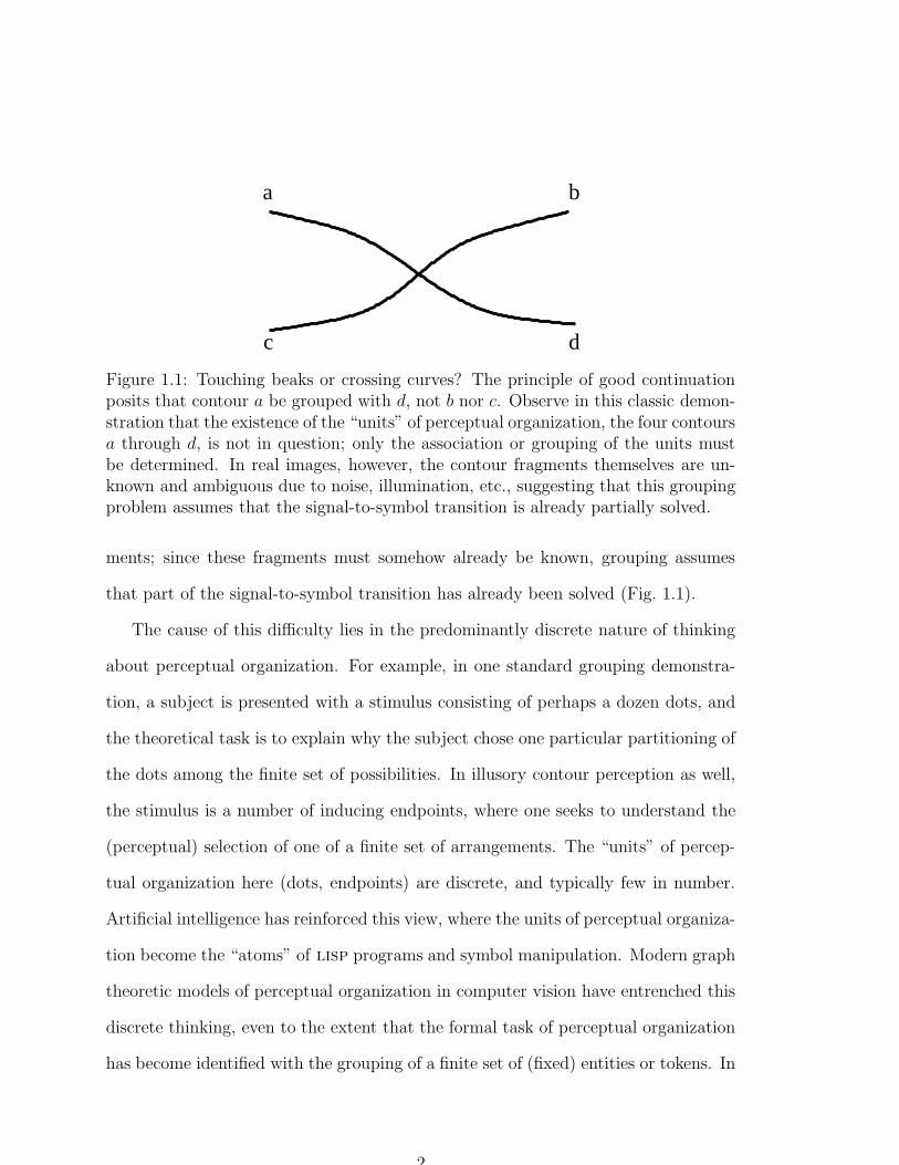
a b

dc

Figure 1.1: Touching beaks or crossing curves? The principle of good continuationposits that contour a be grouped with d, not b nor c. Observe in this classic demon-stration that the existence of the “units” of perceptual organization, the four contoursa through d, is not in question; only the association or grouping of the units mustbe determined. In real images, however, the contour fragments themselves are un-known and ambiguous due to noise, illumination, etc., suggesting that this groupingproblem assumes that the signal-to-symbol transition is already partially solved.

ments; since these fragments must somehow already be known, grouping assumes

that part of the signal-to-symbol transition has already been solved (Fig. 1.1).

The cause of this difficulty lies in the predominantly discrete nature of thinking

about perceptual organization. For example, in one standard grouping demonstra-

tion, a subject is presented with a stimulus consisting of perhaps a dozen dots, and

the theoretical task is to explain why the subject chose one particular partitioning of

the dots among the finite set of possibilities. In illusory contour perception as well,

the stimulus is a number of inducing endpoints, where one seeks to understand the

(perceptual) selection of one of a finite set of arrangements. The “units” of percep-

tual organization here (dots, endpoints) are discrete, and typically few in number.

Artificial intelligence has reinforced this view, where the units of perceptual organiza-

tion become the “atoms” of lisp programs and symbol manipulation. Modern graph

theoretic models of perceptual organization in computer vision have entrenched this

discrete thinking, even to the extent that the formal task of perceptual organization

has become identified with the grouping of a finite set of (fixed) entities or tokens. In

2

these discrete “symbolic” models, the underlying presence of a signal—the image—is

suppressed.

Unfortunately, natural images are ambiguous, and not only in terms of the group-

ings of discrete units: even the existence or absence of these units is uncertain. For

the inference of contour structure, this ambiguity implies that the true space of units

is the uncountably infinite set of all possible curve groups; explicitly enumerating

them is unthinkable. To cross this both semantic and now practical divide between

images and contours, we introduce an intermediate structure—the curve indicator

random field—which will allow us to bring perceptual organization closer to signal

processing by formalizing what one can mean by an image of curves. In particular,

we shall study and exploit the statistical structure of this field and then derive filters

for extracting contour information from noisy images.

To motivate our model, consider the situation of an artist sketching a scene.

Using a pen, the artist draws contours on the paper; this motion can be formalized

mathematically as a curve, or mapping of a parameter, the current time in the

duration of the stroke, to the point in the plane where the tip of the pen is located1. A

separate time-sequence of pen locations can be recorded for each stroke; together this

set of curves provides a description of the artist’s activity. Another way of describing

this situation is the drawing itself; the ink records a trace of the pen’s motion, but

discards the curves’ parameterizations. The drawing might be called an “ink field,”

where the value of the field at a point specifies how much ink was deposited there;

this field has zero value except along the sketched contours. Combined with the

randomness inherent in the act of drawing, this ink field will inspire our definition

1Such pen motion is actually recorded in current hand-held electronic pen devices such as thePalm Pilot.

3

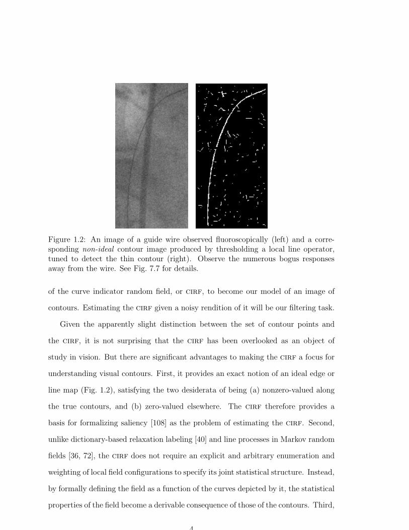
Figure 1.2: An image of a guide wire observed fluoroscopically (left) and a corre-sponding non-ideal contour image produced by thresholding a local line operator,tuned to detect the thin contour (right). Observe the numerous bogus responsesaway from the wire. See Fig. 7.7 for details.

of the curve indicator random field, or cirf, to become our model of an image of

contours. Estimating the cirf given a noisy rendition of it will be our filtering task.

Given the apparently slight distinction between the set of contour points and

the cirf, it is not surprising that the cirf has been overlooked as an object of

study in vision. But there are significant advantages to making the cirf a focus for

understanding visual contours. First, it provides an exact notion of an ideal edge or

line map (Fig. 1.2), satisfying the two desiderata of being (a) nonzero-valued along

the true contours, and (b) zero-valued elsewhere. The cirf therefore provides a

basis for formalizing saliency [108] as the problem of estimating the cirf. Second,

unlike dictionary-based relaxation labeling [40] and line processes in Markov random

fields [36, 72], the cirf does not require an explicit and arbitrary enumeration and

weighting of local field configurations to specify its joint statistical structure. Instead,

by formally defining the field as a function of the curves depicted by it, the statistical

properties of the field become a derivable consequence of those of the contours. Third,

4

being a field, the cirf makes it possible to formalize what is even meant by observing

contours under various forms of corruption. Without the cirf, a concept of a noisy

contour might mean a smooth curve made rough; with the cirf, a noisy image

of a contour is simply the pointwise addition of one field (the cirf) with another

(white noise), for example. Fourth, the filters we derive provide a different notion of

blur scale than convolution by a Gaussian, or linear scale-space [59]. In particular,

smoothing will take place along the (putative) contours. Finally, the cirf provides a

local representation of a global curve property: intersection. As ink builds up where

contours cross in a sketch, so does the value of the cirf increase at intersections.

There are two major sources of inspiration for this work. The first is the set of

relaxation labeling [102] approaches to contour computation, which explicitly empha-

sized the need to include contextual interaction in inference, in contrast to classical

edge detection techniques that regard each edge independently (followed by a link-

ing procedure perhaps) [11]. Based on optimization [47] and game theory [78], these

approaches formalize contour inference as a labeling problem using a notion of label

compatibility derived from good continuation formalized using orientation [139] or

co-circularity [89, 49]. The second source of inspiration is the work on curves of least

energy [43] or elastica [82] and its probabilistic expression as stochastic completion

fields [126]. We have introduced the cirf to unify these works in a probabilistic

framework.

This thesis is organized as follows. Because the signal-to-symbol transition is

fraught with uncertainty, we shall use probabilistic techniques throughout. We be-

gin in Chapter 2 with a review of Markov process models of the random contours

that will drive the cirf model. There we shall observe two key random models of

good continuation, the first based on the local tangent direction, and the second

based on curvature. Given a random contour model, we then formally define the

5

cirf in Chapter 3. In the case of Markov process contour models, we then derive

explicit formulas for the moments and cumulants of the cirf, in the single-curve

and multiple-curve cases, respectively, and summarize this joint statistical structure

with a tractable expression for the cirf moment generating functional. In Chap-

ter 4 we briefly observe that our model is not arbitrary by presenting empirical edge

correlations from several natural images that agree with the correlations of the cirf.

Chapter 5 explores how we can exploit the statistics of the cirf to derive filters by

solving an estimation problem. The chapter begins with a review of Bayes decision

theory, arguing for an additive loss function and leading to minimum mean-square

error estimation of the cirf given a corrupted image of it. After describing some

practical observation models, or likelihoods, we then attack the core filtering problem

of computing the posterior mean of the cirf. Since we are primarily interested in

filtering in high noise situations where the ambiguity is greatest, we derive linear,

quadratic, and cubic Volterra filters by taking a perturbation expansion around an

infinite noise level; we employ a novel diagram technique to facilitate the lengthy

hand calculations. Another class of filters is derived by approximating the poste-

rior with a more manageable distribution, the biased cirf. As a result we obtain

(discrete approximations to) a coupled pair of reaction-diffusion-convection integro-

elliptic partial differential equations (pdes) for estimating the posterior mean. Nu-

merical techniques for computing solutions to our filters are presented in Chapter 6,

and experimental results are provided in Chapter 7. Our results demonstrate a strik-

ing ability of our filters for enhancing contour structure in noisy images, including

the guide wire of Fig. 1.2. The results also show that filters are orientation- and

curvature-selective. We conclude and suggest future work in Chapter 8.

6

1.1 Contributions

In this thesis, we present a number of results and novel ideas for understanding and

inferring curve structure in images. Specifically, we

• Introduce the curve indicator random field as an ideal edge/line map. We sug-

gest that the statistical regularities of the cirf can be exploited for enhancing

noisy edge/line maps. The cirf is applicable even if the individual contours

are neither Markovian nor independent;

• Prove an accessible proof of the Feynman-Kac formula for discrete-space Markov

processes, leading to the moments of the single-curve cirf;

• Derive the cumulants and a tractable form for the moment generating func-

tional of the multiple-curve cirf.

• Show that the curve indicator random field is non-Gaussian;

• Introduce a curvature-based Markov process as a model of smooth contours.

We prove that the most probable realization of this process is an Euler spiral;

• Formalize the problem of optimal contour inference (given a corrupted image)

as the minimum-mean square estimate (mmse) of the cirf;

• Derive novel high-noise linear, quadratic and cubic Volterra mmse cirf filters

with low computational complexity. The derivation exploits a novel diagram

construction;

• Compute the cumulants of a biased cirf and derived mmse cirf filters by ap-

proximating the cirf posterior with a biased cirf. This leads to new nonlinear

contour filtering equations;

7

• Develop a rapid, accurate method for applying the Green’s operator of a

direction-based Markov process. Previous techniques were either very expen-

sive or inaccurate. This technique is also extended to the curvature Markov

process;

• Develop numerical techniques for solving the filtering equations;

• Apply these filters to noisy synthetic and real images, demonstrating significant

contour enhancement; and

• Compute edge correlations and observe a connection to the correlations of the

cirf.

8

Chapter 2

Markov Processes for Vision

What class of contour models is broad enough to capture curve properties relevant

for vision and yet both mathematically and computationally tractable? We start

this chapter by arguing that Markov processes generally satisfy these needs, while

acknowledging situations where they do not. We then review the theory of Markov

processes and a process by Mumford [82] that represents the basic local geometry

of a curve up to its tangent. Because curvature is also significant in vision, we then

introduce a Markov process in curvature. Finally, we suggest other Markov processes

that are useful for vision.

We now establish some notation and terminology. Recall that a planar curve is

a function taking a parameter t ∈ to a point γ(t) := (x(t), y(t)) in the plane

2.

(Also recall that the notation A := B means that the symbol A is defined as the

expression B, whereas A =: B means the opposite.) The local tangent vector (x, y)

has direction θ,1 defined as θ := arg(x +y), where

is the imaginary unit

√−1,

the dot denotes differentiation with respect to the arc-length parameter t, and arg z

denotes the counterclockwise angle from the real axis to z in the complex plane.

1Directions are angles over the circle [0, 2π), while orientations are angles over the half-circle[0, π).

9

Without loss of generality, we assume that the tangent (x, y) (where it exists) has

unit length, i.e., x2+y2 = 1. Curvature κ is equal to θ, the rate of change of direction.

Into this deterministic picture we now inject the uncertainty of vision: since

images are ambiguous, so too will be the structures within it. In other words, any

given structure in a particular image can be viewed as a realization of a random

variable.2 In this way, any given curve γ is thus a realization of a random curve Γ.3

Since Γ = Γ(t) is a one-parameter family of random planar vectors, Γ is a random

process by definition.

2.1 Why Markov Processes?

By making randomness explicit, we clear a path for overcoming it. While the true

curve is uncertain, the curve random process has a lawful distribution that can be

exploited to support contour inferences. Put loosely, we can bias our inferences

towards the probable curves and away from the rare. The rich variety of possible

image curves may appear to suggest, however, that the structure of this distribution

is either too simple to be useful (e.g., “uniform”) or too complex to be practical

(i.e., an arbitrary distribution over the infinite-dimensional space of distributions of

functions). As suggested by the Gestalt law of good continuation, the truth lies is

somewhere in between: although many contours can occur, most have some regular

structure; e.g., object boundaries usually have a degree of smoothness. The class

of Markov processes is ideal for describing such local statistical regularity of visual

curves, while remaining tractable.

2A random variable may be a scalar, vector or function (i.e., a process or field). A randomprocess has only one parameter, while a random field generally has several.

3We often will use upper and lower case letters to denote random variables and their realizations(samples), respectively. Capitals also denote operators later in this thesis.

10

[ ]0 Tt

θ

y

xRt

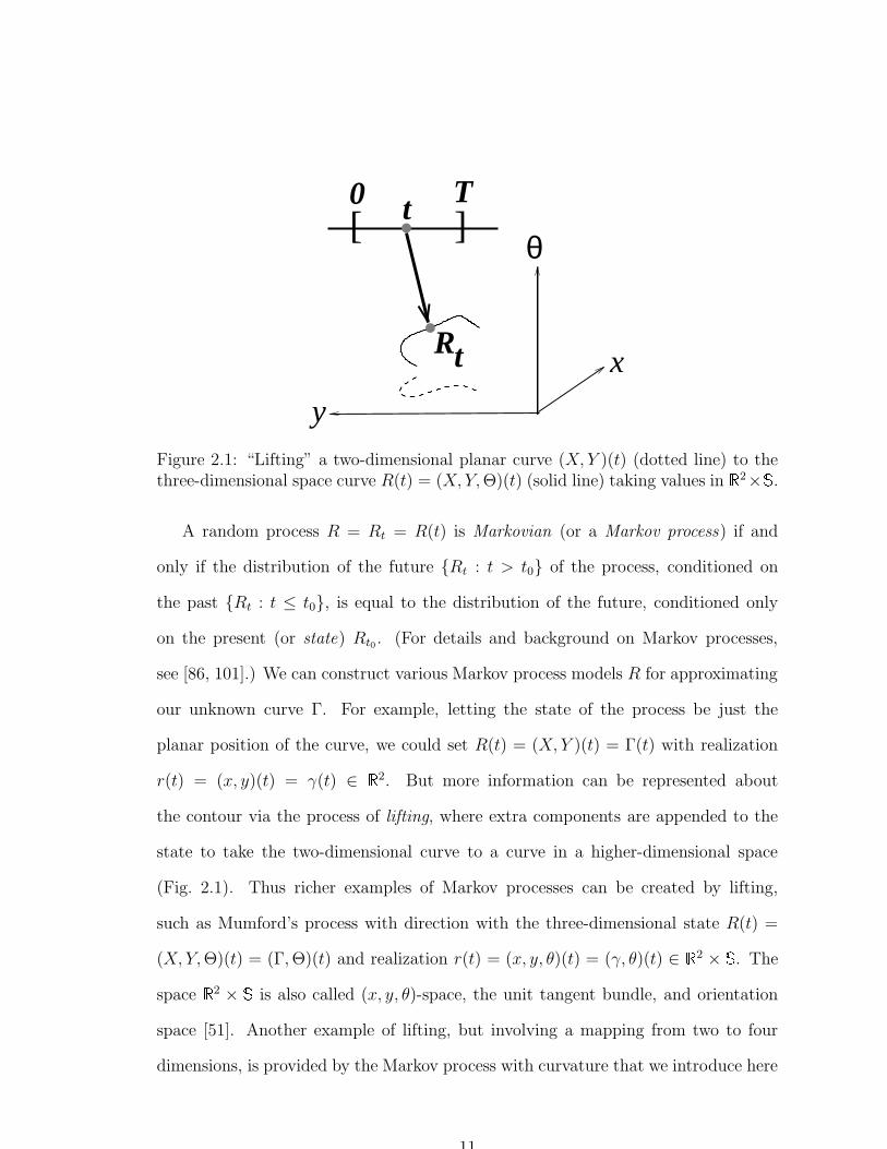
Figure 2.1: “Lifting” a two-dimensional planar curve (X, Y )(t) (dotted line) to thethree-dimensional space curve R(t) = (X, Y,Θ)(t) (solid line) taking values in

2× .

A random process R = Rt = R(t) is Markovian (or a Markov process) if and

only if the distribution of the future Rt : t > t0 of the process, conditioned on

the past Rt : t ≤ t0, is equal to the distribution of the future, conditioned only

on the present (or state) Rt0 . (For details and background on Markov processes,

see [86, 101].) We can construct various Markov process models R for approximating

our unknown curve Γ. For example, letting the state of the process be just the

planar position of the curve, we could set R(t) = (X, Y )(t) = Γ(t) with realization

r(t) = (x, y)(t) = γ(t) ∈ 2. But more information can be represented about

the contour via the process of lifting, where extra components are appended to the

state to take the two-dimensional curve to a curve in a higher-dimensional space

(Fig. 2.1). Thus richer examples of Markov processes can be created by lifting,

such as Mumford’s process with direction with the three-dimensional state R(t) =

(X, Y,Θ)(t) = (Γ,Θ)(t) and realization r(t) = (x, y, θ)(t) = (γ, θ)(t) ∈ 2 × . The

space 2 × is also called (x, y, θ)-space, the unit tangent bundle, and orientation

space [51]. Another example of lifting, but involving a mapping from two to four

dimensions, is provided by the Markov process with curvature that we introduce here

11

with R(t) = (X, Y,Θ, K)(t) = (Γ,Θ, K)(t) with realization r(t) = (x, y, θ, κ)(t) =

(γ, θ, κ)(t) ∈ 2 × × . These examples show that not only can the present state4

R(t) of the Markov process represent the present value Γ(t) of the unknown curve,

it also can capture (uncertain) local differential information such as direction and

curvature. In addition to the curve’s local geometry, the state can represent other

local information such as blur scale [116], intensity (on one or both sides of the

curve), contrast, color, texture, material information, edge classification (edge vs.

line, etc.), and indeed any property that is locally definable.

Merely setting up the state vector is insufficient to characterize a Markov process:

the transition probabilities are also necessary. Such probabilities describe how the

present state influences the future; for visual contours, the transition probabilities

therefore model how local properties extend along the curve. For example, in a

world of infinitely long straight lines, the local position and direction determine

those elsewhere along the curve; additionally including curvature is not necessary.

For a world of very smooth contours, higher-derivative information than curvature

may reliably predict nearby positions along the curves. But for fractal boundaries,

even local direction would be a poor predictor of the contour nearby a point along the

curve. Transition probabilities can model all of these situations, and can therefore be

used to gauge the usefulness of particular local properties: those that “persist” for

some distance along the curve will support the inference of these curves that we study

in Chapter 5. In a sense, Markov processes both formalize the Gestalt concept of

good continuation and generalize it to non-geometrical visual cues such as contrast;

the transition probabilities quantitatively characterize the relative power of these

cues. Markov processes are not even limited to the modeling of such generalized

4In a discrete-time setting there is the distinction between first-order and higher-order processes;by a suitable change of state space this distinction is irrelevant and so we consider first-order Markovprocesses only.

12

good continuations; they can also specify how good continuations break down, e.g.,

at discontinuities (see §2.5).

Desolneux et al take a different view on contour properties: they emphasize

properties that curves do not have, instead of those they do [17, 18]. Instead of fixing

a distribution over the smoothness of a curve (as represented via a Markov process,

for example), they view smoothness as a rare (and thus meaningful) deviation from

uniform randomness (contour roughness, for example).

2.1.1 Limitations of Markov Processes

While Markov processes do capture a variety of crucial properties of contours, it

is important to realize that non-local cues are not explicitly included, such as clo-

sure, symmetry, simplicity (no self-intersections), and junctions (intersections be-

tween possibly distinct contours). The fundamental difficulty with all of these prop-

erties is their global nature: for a random process with any of these properties, the

entire process history directly influences the future. For a Markov process, however,

only the present state directly affects the future; the past has only indirect effects.

Fortunately, there are several tools using which we can exploit global contour prop-

erties without abandoing Markov processes: spectral techniques, alternative shape

representations, and the curve indicator random field (§3.1.1).

To study and extract closed contours, Mahamud, Williams and Thornber com-

bined a Markov process boundary model with spectral analysis [70]. They viewed

closed curves as being infinitely long; the curve repeatedly cycles through the same

points. This cycling was formalized as an eigenvalue problem as follows. After ex-

tracting locally-detected edges, they constructed a reduced state-space consisting

of the positions and possible directions of a subsampling of these edges. Then the

eigenvector corresponding to the maximum positive eigenvalue for a (function of) the

13

process’s transition matrix was computed. They argued that the largest elements

of this eigenvector can be interpreted as lying on a smooth closed curve, and so

they iteratively removed closed curves from images by thresholding out these large

elements and re-computing the maximum eigenvector for the remaining edges. In

§8.1 we suggest another way to represent both symmetry and closure using a Markov

process model of the skeleton representation of the boundary.

Two other global contour properties are simplicity and junctions. For example,

given a parameterization of the contour, one has to traverse the entire domain of

parameterization to determine whether the contour crossed itself [80]. As we shall

see in §3.1.1, this global computation in terms of the parameterization becomes local

in terms of the cirf. Enforcing this constraint is discussed in §5.2, and violations

of the constraint are penalized by filters that we derive in Chapter 5. Junctions

represent contour crossings as well, but of distinct curves, and also are a global

property of the contour parameterizations. Both of these global contour properties

become local properties of a field.

So we see that while Markov processes in themselves do not convey global contour

properties, they are not incompatible with global contour information when captured

appropriately. We now consider one other global contour property: length.

2.1.2 Length Distributions

Not only do contours vary in their local properties, they also vary in length. While

one may consider a large variety of length distributions, as a first approximation

we assert a memoryless property: whether the contour continues beyond a certain

point does not depend on how long it already is. We also assume that the length

is independent of other aspects of the contour. This implies an exponential density

pT (t) = α exp(−αt) for the unknown contour length T , where λ := α−1 is the average

14

contour length. This length distribution is equivalent to a constant killing (or decay

rate) α at each point in the state-space (see 2.6). This length distribution was used

in [82] and [126].

One may view the exponential distribution over contour length as conservative

in two respects. First, the memoryless property is an independence assumption: the

probability that the curve will continue for a certain length is independent of its

current length. Second, the exponential distribution can be used to represent highly

ambiguous lengths. Consider what occurs as λ is increased to infinity: the slope

of the density becomes increasingly flat, and so the length distribution increasingly

appears uniform over any given length interval.

To model more general length distributions we can consider either (1) non-

stationary Markov processes on the same state-space or (2) stationary Markov pro-

cesses on an augmented state-space. As we shall require stationarity in Chapter 3,

we could still take the second approach where we would add a length component to

the state vector and modify the transition probabilities to monotonically increase the

length component with process time. Richer length distributions would be captured

by a non-constant decay rate, i.e., killing depends on the length component of the

state. For example, to bias toward curves with length less than t∗ one would have a

small killing rate for states with length component less than t∗, and a large killing

rate for states with a large length component.

With this capacity for more varied length distributions, we continue our presen-

tation of stationary Markov processes with exponentially distributed lengths. We

shall concentrate on contour geometry in continuous spaces; later we discretize in

preparation for the formal development of the contour filters we derive in Chapter 5.

15

2.2 Planar Brownian Motion

Perhaps the simplest contour model is Brownian motion in the plane. Although we

shall not be using it in our filters, Brownian motion is historically important and

forms a benchmark for more complex random processes. Intuitively, it can represent

the random motion of microscopic particles. Mathematically, we can use the notation

of stochastic differential equations (sdes) to describe planar Brownian motion as the

random process R(t) = (X, Y )(t) such that

dX = σ dW (1), dY = σ dW (2), (2.1)

where W (1) and W (2) are independent, standard Brownian motions5 and σ = σBM >

0 is the “standard deviation in the derivatives”. Planar Brownian motion is an

example of a diffusion process and is characterized by the transition probability

pR(t)|R(0)(r, t|r0), which is the conditional probability density that the particle is lo-

cated at r at time t given that it started at r0 at time 0. We write the transition

probability as p = p(x, y, t) = pR(t)|R(0)(r|r0), where r0 := (x0, y0) is the initial posi-

tion of the process, and they satisfy the following Fokker-Planck diffusion equation:

∂p

∂t= Lp, where L =

σ2

2

(∂2

∂x2+

∂2

∂y2

)=σ2

2∆, (2.2)

where the initial condition is pR(0)(r) = δ(r − r0) = p(x, y, 0) = δ(x − x0)δ(y − y0),

δ(x) is the Dirac δ-distribution6 and the spatial boundary conditions must be appro-

priately specified. The partial differential operator L is known as the (infinitesimal)

generator of the Markov process and fully characterizes the infinitesimal motion

5For reference, a standard Brownian motion W is a stationary (continuous) Markov process on

where the increments are independent and increment Wt −Wt′ is a zero-mean Gaussian randomvariable of variance |t− t′|.

6δ(x) is also called a Dirac δ-function.

16

of the particle’s probability density. The other Markov processes we shall see are

distinguished by their generators.

While Brownian motion has the advantage of capturing the continuity of contours

(since realizations are continuous), it has two difficulties for vision. First, sample

paths of Brownian motion frequently self-intersect. Not only does this not correspond

to actual contours in the world, it also makes the job of filtering more difficult, as

we shall see in §5.5. Second, planar Brownian motion does not represent the local

geometry of contours. In particular, since Brownian paths are differentiable almost-

nowhere, the tangent does not exist (except on a set of measure zero). Thus planar

Brownian motion is a poor model of good continuation, elongated receptive fields

in the visual cortex [45], and the observed edge statistics in natural images (see

Chapter 4), where tangent information is important. The need to capture the local

geometry of contours leads us to more elaborate Markov processes.

2.3 Brownian Motion in Direction

To motivate their model for local contour smoothness, first Mumford [82], and later

Williams and co-workers [126], imagined a particle at R(t) = (Xt, Yt,Θt) ∈ 2 ×

whose direction Θt is slightly perturbed at each time instant t before taking its next

step forward. Mathematically, this particle can be described by a Markov process

with the stochastic differential equation

dX

dt= sin Θ,

dY

dt= cos Θ, dΘ = σdW, (2.3)

where σ = σκ bounds the direction perturbations and W is standard Brownian

motion (on the circle ). In this way a fundamental descriptor of the local geometry

17

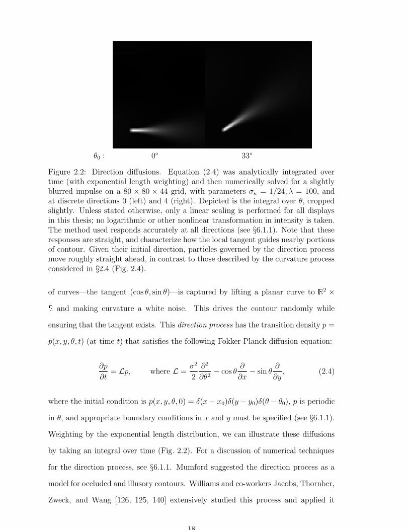
θ0 : 0 33

Figure 2.2: Direction diffusions. Equation (2.4) was analytically integrated overtime (with exponential length weighting) and then numerically solved for a slightlyblurred impulse on a 80 × 80 × 44 grid, with parameters σκ = 1/24, λ = 100, andat discrete directions 0 (left) and 4 (right). Depicted is the integral over θ, croppedslightly. Unless stated otherwise, only a linear scaling is performed for all displaysin this thesis; no logarithmic or other nonlinear transformation in intensity is taken.The method used responds accurately at all directions (see §6.1.1). Note that theseresponses are straight, and characterize how the local tangent guides nearby portionsof contour. Given their initial direction, particles governed by the direction processmove roughly straight ahead, in contrast to those described by the curvature processconsidered in §2.4 (Fig. 2.4).

of curves—the tangent (cos θ, sin θ)—is captured by lifting a planar curve to 2 ×

and making curvature a white noise. This drives the contour randomly while

ensuring that the tangent exists. This direction process has the transition density p =

p(x, y, θ, t) (at time t) that satisfies the following Fokker-Planck diffusion equation:

∂p

∂t= Lp, where L =

σ2

2

∂2

∂θ2− cos θ

∂

∂x− sin θ

∂

∂y, (2.4)

where the initial condition is p(x, y, θ, 0) = δ(x− x0)δ(y − y0)δ(θ− θ0), p is periodic

in θ, and appropriate boundary conditions in x and y must be specified (see §6.1.1).

Weighting by the exponential length distribution, we can illustrate these diffusions

by taking an integral over time (Fig. 2.2). For a discussion of numerical techniques

for the direction process, see §6.1.1. Mumford suggested the direction process as a

model for occluded and illusory contours. Williams and co-workers Jacobs, Thornber,

Zweck, and Wang [126, 125, 140] extensively studied this process and applied it

18

to modeling illusory contours using the stochastic completion field and modeling

closed contours using spectral analysis (see §5.8 for comparison to the cirf). The

covariances of the curve indicator random field (Corollary 4 and Fig. 3.2) based on the

direction process also resemble several formalizations of good continuation [139, 29]

and horizontal interactions in the visual cortex [138].

As Mumford has shown [82], the mode of the distribution of this direction pro-

cess is described by an elastica, or that planar curve which minimizes the following

functional: ∫(βκ2 + α) dt, (2.5)

where β = (2σ2)−1 and α = λ−1 is the constant killing. The elastica functional

measures the bending-energy of thin splines, and was first studied by Euler [28].

Mumford derived formulas for elastica in terms of theta functions. In computer

vision, elasticae were used to model illusory contours and the completion of boundary

gaps [122, 43, 85].

2.4 Brownian Motion in Curvature

Inspired by Gestalt psychology [61], most previous studies of contour smoothness

have focused on good continuity in orientation, that is to say, curves with varying

orientation—high curvature—are rejected, and, conversely, straighter curves are en-

hanced. This is naturally phrased in terms of the elastica functional (2.5) on curves

that minimizes curvature. Now we introduce a Markov process model that instead

aims to enforce good continuation in curvature, and thus minimizes changes in cur-

vature.

19

ab

c

d

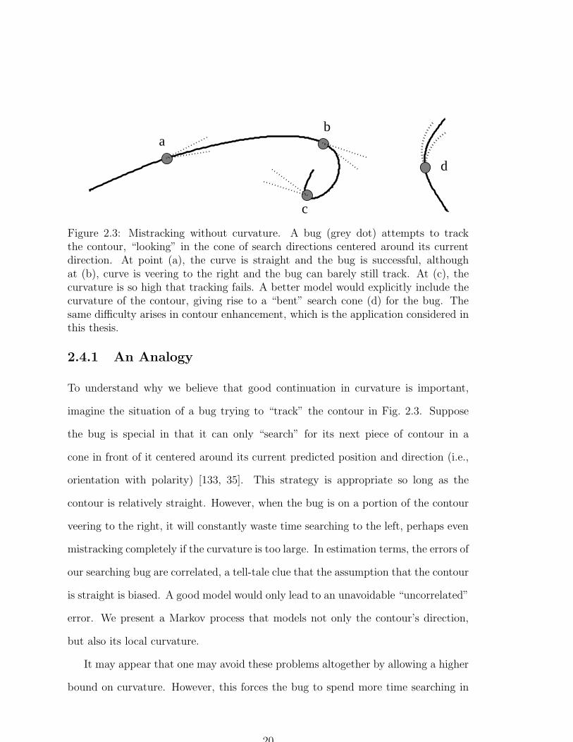
Figure 2.3: Mistracking without curvature. A bug (grey dot) attempts to trackthe contour, “looking” in the cone of search directions centered around its currentdirection. At point (a), the curve is straight and the bug is successful, althoughat (b), curve is veering to the right and the bug can barely still track. At (c), thecurvature is so high that tracking fails. A better model would explicitly include thecurvature of the contour, giving rise to a “bent” search cone (d) for the bug. Thesame difficulty arises in contour enhancement, which is the application considered inthis thesis.

2.4.1 An Analogy

To understand why we believe that good continuation in curvature is important,

imagine the situation of a bug trying to “track” the contour in Fig. 2.3. Suppose

the bug is special in that it can only “search” for its next piece of contour in a

cone in front of it centered around its current predicted position and direction (i.e.,

orientation with polarity) [133, 35]. This strategy is appropriate so long as the

contour is relatively straight. However, when the bug is on a portion of the contour

veering to the right, it will constantly waste time searching to the left, perhaps even

mistracking completely if the curvature is too large. In estimation terms, the errors of

our searching bug are correlated, a tell-tale clue that the assumption that the contour

is straight is biased. A good model would only lead to an unavoidable “uncorrelated”

error. We present a Markov process that models not only the contour’s direction,

but also its local curvature.

It may appear that one may avoid these problems altogether by allowing a higher

bound on curvature. However, this forces the bug to spend more time searching in

20

a larger cone. In stochastic terms, this larger cone is amounts to asserting that the

current (position, direction) state has a weaker influence on the next state; in other

words, the prior on contour shape is weaker (less peaked or broader). But a weaker

prior will be less able to counteract a weak likelihood (high noise): it will not be

robust to noise. Thus we must accept that good continuation models based only on

contour direction are forced to choose between allowing high curvature or high noise;

they cannot have it both ways.7

Although studying curvature is hardly new in vision, modeling it probabilistically

began only recently with Zhu’s empirical model of contour curvature [135]. In [19,

138, 60] and [37, 361 ff.], measuring curvature in images was the key problem. In [58],

curvature is used for smooth interpolations, following on the work on elasticae. The

closest work in spirit to this is relaxation labeling [139], several applications of which

include a deterministic form of curvature [89, 49]. Co-circularity (introduced in [89])

is related to curvature, and was used in Markov random field models for contour

enhancement [42].

We now formally introduce our Markov process in curvature and its diffusion

equation; we then present example impulse responses, which act like the “bent”

search cones. We also relate the mode of the distribution for the curvature process

to an energy functional on smooth curves.

2.4.2 The Mathematics of the Curvature Process

Consider the Markov process that results from making curvature a Brownian motion.

This process has state R(t) = (X, Y,Θ, K)(t), realization r = (x, y, θ, κ) ∈ 2× × ,

7Observe in the road-tracking examples in [35] how all the roads have fairly low curvature. Whilethis is realistic in flat regions such as the area of France considered, others, more mountainousperhaps, have roads that wind in the hillsides.

21

and can be described by the following stochastic differential equation:

dX

dt= cos Θ,

dY

dt= sin Θ,

dΘ

dt= K, dK = σdW, (2.6)

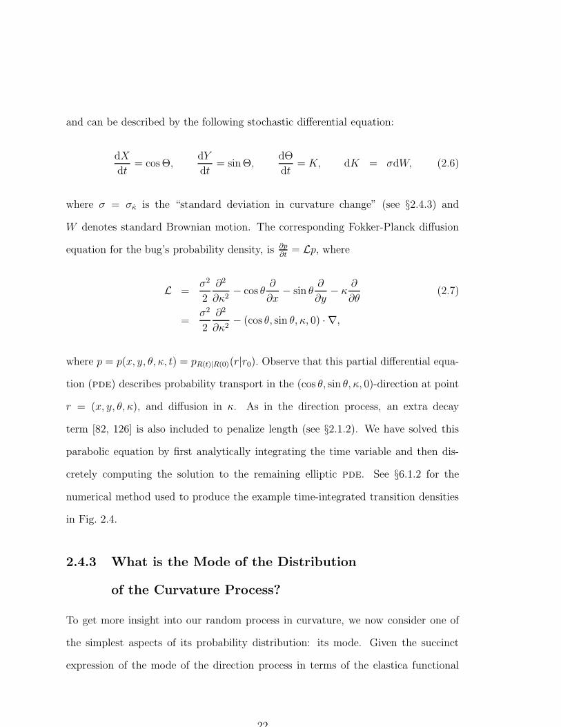
where σ = σκ is the “standard deviation in curvature change” (see §2.4.3) and

W denotes standard Brownian motion. The corresponding Fokker-Planck diffusion

equation for the bug’s probability density, is ∂p∂t

= Lp, where

L =σ2

2

∂2

∂κ2− cos θ

∂

∂x− sin θ

∂

∂y− κ

∂

∂θ(2.7)

=σ2

2

∂2

∂κ2− (cos θ, sin θ, κ, 0) · ∇,

where p = p(x, y, θ, κ, t) = pR(t)|R(0)(r|r0). Observe that this partial differential equa-

tion (pde) describes probability transport in the (cos θ, sin θ, κ, 0)-direction at point

r = (x, y, θ, κ), and diffusion in κ. As in the direction process, an extra decay

term [82, 126] is also included to penalize length (see §2.1.2). We have solved this

parabolic equation by first analytically integrating the time variable and then dis-

cretely computing the solution to the remaining elliptic pde. See §6.1.2 for the

numerical method used to produce the example time-integrated transition densities

in Fig. 2.4.

2.4.3 What is the Mode of the Distribution

of the Curvature Process?

To get more insight into our random process in curvature, we now consider one of

the simplest aspects of its probability distribution: its mode. Given the succinct

expression of the mode of the direction process in terms of the elastica functional

22

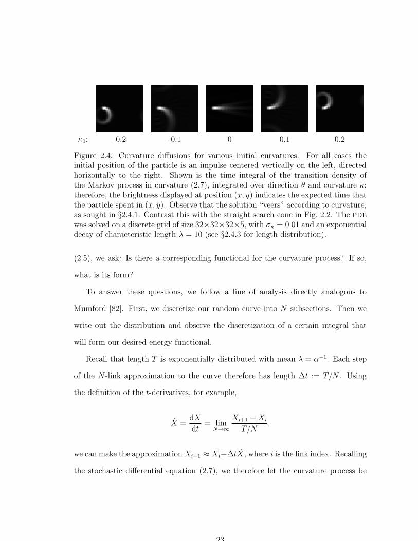
κ0: -0.2 -0.1 0 0.1 0.2

Figure 2.4: Curvature diffusions for various initial curvatures. For all cases theinitial position of the particle is an impulse centered vertically on the left, directedhorizontally to the right. Shown is the time integral of the transition density ofthe Markov process in curvature (2.7), integrated over direction θ and curvature κ;therefore, the brightness displayed at position (x, y) indicates the expected time thatthe particle spent in (x, y). Observe that the solution “veers” according to curvature,as sought in §2.4.1. Contrast this with the straight search cone in Fig. 2.2. The pde

was solved on a discrete grid of size 32×32×32×5, with σκ = 0.01 and an exponentialdecay of characteristic length λ = 10 (see §2.4.3 for length distribution).

(2.5), we ask: Is there a corresponding functional for the curvature process? If so,

what is its form?

To answer these questions, we follow a line of analysis directly analogous to

Mumford [82]. First, we discretize our random curve into N subsections. Then we

write out the distribution and observe the discretization of a certain integral that

will form our desired energy functional.

Recall that length T is exponentially distributed with mean λ = α−1. Each step

of the N -link approximation to the curve therefore has length ∆t := T/N . Using

the definition of the t-derivatives, for example,

X =dX

dt= lim

N→∞

Xi+1 −Xi

T/N,

we can make the approximation Xi+1 ≈ Xi+∆tX, where i is the link index. Recalling

the stochastic differential equation (2.7), we therefore let the curvature process be

23

approximated in discrete time by

Xi+1 = Xi + ∆t cos Θi, Yi+1 = Yi + ∆t sin Θi, Θi+1 = Θi + ∆tKi,

where i = 1, . . . , N . Because Brownian motion has independent increments whose

standard deviation grows with the square root√

∆t of the time increment ∆t, the

change in curvature for the discrete process becomes

Ki+1 = Ki +√

∆t εi,

where εi is an independent and identically distributed set of 0-mean, Gaussian

random variables of standard deviation σ = σκ. Now let the discrete contour be

denoted by

γN = (Xi, Yi,Θi, Ki) : i = 0, . . . , N.

Given an initial point p0 = (x0, y0, θ0, κ0), the probability density for the other points

is

p(γN |p0) = α exp(−αT ) · (√

2πσ)−N exp

(−∑

i

ε2i2σ2

),

which, by substitution, is proportional to

exp

[−∑

i

1

2σ2

(κi+1 − κi

∆t

)2

∆t− αT

].

We immediately recognize κi+1−κi

∆tas an approximation to dκ

dt= κ, and so we conclude

that

p(γN |p0) → p(γ|p0) ∝ e−E(γ) as N →∞,

24

where the energy E(γ) of (continuous) curve γ is

E(γ) =

∫(βκ2 + α) dt, (2.8)

and where β = (2σ2)−1 and α = λ−1.

Maximizers of the distribution p(γ) for the curvature random process are planar

curves that minimize the functional E(γ), which we call the Euler spiral functional.

When α = 0—when there is no penalty on length—, such curves are known as

Euler spirals, and have been studied recently in [58]. A key aspect of the Euler

spiral functional (2.8) is that it penalizes changes in curvature, preferring curves

with slowly varying curvature. In contrast, the elastica functional (2.5) penalizes

curvature itself, and therefore allows only relatively straight curves, to the dismay

of the imaginary bug of §2.4.1. This Euler spiral energy is also loosely related to

the notion of co-circularity expressed in [49]: the coefficient β would play a role of

weighting the “compatibility distance” between a pair of sites (x, y, θ, κ), curvature

while the coefficient α would affect the “transport distance” between them. In other

words, the integral over κ2 in E(γ) is a measure of how non-co-circular two tangents

are, while the second integral measures how far apart they are, defined as the length

of γ, the smooth curve joining them.

2.5 Other Markov Process Models

At the start of this chapter we suggested the use of Markov processes for a host of

contour cues other than the local geometry captured by the direction and curvature

processes. The simplest way of extending a Markov process to include this extra in-

formation, say contrast C, is to add a component to the state vector and assume that

25

it is a Brownian motion independent of the geometry and other factors. Smoothness

in C can be enforced by letting the derivative C be a Brownian motion (or even

the Ornstein-Uhlenbeck [121, 82] process suggested in 3-dimensions next), and then

appending two components to the state vector (one for the contrast itself, the other

for its derivative). Even dependencies among different sources of information, say

intensity and geometry, can be modeled using Markov processes, but this is more

complex.

While the emphasis in this thesis lies in fully exploiting the local properties of

curves in the plane, the framework applies unmodified to higher dimensional images.

In medical imaging of vascular structures in cat and mri images, one would require

random process models of 3-dimensional space curves. With appropriate observation

models (see §5.2), this framework could also be exploited for binocular stereo or even

multiview reconstruction of space curves. In these 3-dimensional applications, one

could exploit a number of properties similar to the 2-dimensional examples we have

discussed. To enforce only continuity one could set the Markov process R(t) =

(X, Y, Z)(t) = (X (1), X(2), X(3))(t) to the spatial Brownian motion

dX(i) = σ dW (i), i = 1, 2, 3,

where W (i) : i = 1, 2, 3 are independent, standard Brownian motions. For a

random 3-dimensional space curve with smoothness up to the local tangent (similar

to the (planar) direction process of §2.3), Mumford suggested a Markov process

obtained by integrating a Brownian motion on 2 (the sphere of unit-length tangent

vectors) [82]. A simpler model would not enforce the unit-length constraint for the

tangent vector; instead, the tangent could be 3-dimensional Brownian motion. A

slightly more general version of this idea includes a force (of spring constant ε) to

26

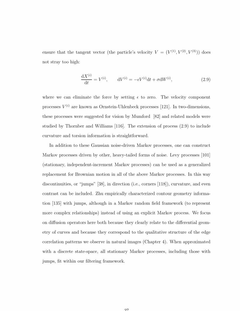
ensure that the tangent vector (the particle’s velocity V = (V (1), V (2), V (3))) does

not stray too high:

dX(i)

dt= V (i), dV (i) = −εV (i)dt + σdW (i), (2.9)

where we can eliminate the force by setting ε to zero. The velocity component

processes V (i) are known as Ornstein-Uhlenbeck processes [121]. In two-dimensions,

these processes were suggested for vision by Mumford [82] and related models were

studied by Thornber and Williams [116]. The extension of process (2.9) to include

curvature and torsion information is straightforward.

In addition to these Gaussian noise-driven Markov processes, one can construct

Markov processes driven by other, heavy-tailed forms of noise. Levy processes [101]

(stationary, independent-increment Markov processes) can be used as a generalized

replacement for Brownian motion in all of the above Markov processes. In this way

discontinuities, or “jumps” [38], in direction (i.e., corners [118]), curvature, and even

contrast can be included. Zhu empirically characterized contour geometry informa-

tion [135] with jumps, although in a Markov random field framework (to represent

more complex relationships) instead of using an explicit Markov process. We focus

on diffusion operators here both because they clearly relate to the differential geom-

etry of curves and because they correspond to the qualitative structure of the edge

correlation patterns we observe in natural images (Chapter 4). When approximated

with a discrete state-space, all stationary Markov processes, including those with

jumps, fit within our filtering framework.

27

2.6 A Working Formalism: Continuous-Time,

Discrete-State Markov Processes

Having set out the kind of processes we shall ultimately use as uncertain contour

models, we need to transition from continuous state-spaces to discrete ones that will

support computations relevant for digital images. In this section we therefore briefly

establish the notation and basic theory of discrete-state Markov processes.

With a slight abuse of notation, we let Rt, where 0 ≤ t < T , denote any stationary

continuous-time Markov process taking values in a finite set I of cardinality |I|. Sites

or states within I will be denoted i and j. We view I as a discrete approximation to

our continuous state-spaces 2× ,

2× × , etc., where our contour random pro-

cesses takes values. For example, (discrete) state i would represent some continuous

state (x, y, θ) for the direction process, and Rt denotes the (discrete) curve Markov

process. As in §2.1.2, the random variable T is exponentially-distributed with mean

value λ, and represents the approximate length of the contour. To ensure finiteness

of the expressions in Chapter 3, we further assume λ <∞.

The (discrete-space) generator of the Markov process Rt is the |I| × |I| matrix

L = (lij), and is the instantaneous rate of change of the probability transition matrix

P (t) = (pij)(t) for Rt. Since we assume that the Markov process is stationary, the

generator L does not vary with time t. One can obtain the discrete-space generator L

by discretizing the continuous-space generator L appropriately; details are provided

in §6.1.

To enforce the exponential distribution over lifetime (length) T of each particle,

we construct a killed Markov process with generator Q = L−αI, where α := λ−1 as

in §2.1.2. (Formally, we do this by adding a single “death” state

to the discrete

state space I. When t ≥ T , the process enters

and it cannot leave.) Slightly

28

changing our notation again, we shall now use Rt to mean the killed Markov process

with generator Q.

The Green’s operator8 G = (gij) of the (killed) Markov process is the matrix

∫∞0eQtdt =

∫∞0P (t)e−αtdt, where P (t) = eLt (eA denotes the matrix exponential of

matrix A). The (i, j)-entry gij in the Green’s matrix represents the expected amount

of time that the Markov process Rt spent in j (before death) given that the process

started in i. The following is a well-known connection between the generator Q

(an approximate differential operator) and the Green’s operator G (an approximate

integral operator):

Lemma 1. G = −Q−1.

proof. Recall the standard result that ddt

eQt = Q eQt, which can be obtained by

using the definition of the matrix exponential as an infinite sum, then differentiating

term by term, and finally re-summing to get back a matrix exponential. We integrate

this from t = 0 to t = ∞: on the left side, we get eQt |∞t=0 = −I; on the right, we get

Q∫∞0

eQt dt = QG.

Having studied (parameterized) contour models, we remove the parameterization

in the next chapter to construct our prior for contour inference from images.

8Formally, G is the Green’s operator (or Green’s matrix) when α = 0, and is known as theresolvent, resolvent matrix, or resolvent operator for α ≥ 0.

29

Chapter 3

The Curve Indicator

Random Field

Given a Markov process for modeling individual contours, we now define a curve indi-

cator random field (cirf), which naturally captures the notion of an ideal edge/line

map. Roughly, this random field is non-zero-valued along the true contours, and

zero-valued elsewhere. The actually measured edge/line map is then viewed as an

imperfect cirf, corrupted by noise, blur, etc. Because the cirf is not standard, our

presentation will be self-contained.

Several independence assumptions play a role in our model. First, we use a mem-

oryless property on contour length T (§2.1.2), which led to an exponential density for

T . Second, we observe that independence of contours is a reasonable approximation

for modeling elongated curves. Tree branch contours, for example, statistically in-

teract primarily where they meet; due to the local process of growth, the individual

branches wander largely independently. Occlusion is apparently a counter-example,

although if we were interested in an “x-ray” view of contour structure, independence

may still be a useful approximation. (We shall weaken the independence assumption

30

in §3.1.1, where contour interactions are described.) Finally, the unknown number

of contours is assumed to be Poisson-distributed: in the related context of random

point fields, this distribution is natural where disjoint regions contain independent

numbers of points. That such assumptions are reasonable can be seen in Fig. 3.1.

3.1 Defining the CIRF

Following §2.6, we focus on continuous-time, discrete-state stationary killed Markov

processes Rt, where 0 ≤ t < T . Let condition denote the (indicator) function

that takes on value 1 if condition is true, and the value 0 otherwise. With this

notation, we can define the curve indicator random field V for a single curve as

Vi :=

∫ T

0

Rt = idt, ∀i ∈ I.

Observe that Vi is the (random) amount of time that the Markov process spent in

state i. In particular, Vi is zero unless the Markov process passed through site i. In

the context of Brownian motion or other symmetric processes, V is variously known

as the occupation measure or the local time of Rt [22, 23, 30].

Generalizing to multiple curves, we pick a random number N and then choose

N independent copies R(1)t1 , . . . , R

(N )tN

of the Markov process Rt, with independent

lengths T1, . . . , TN , each distributed as T . To define the multiple curve cirf, we

take the superposition of the single-curve cirfs V (1), . . . , V (N ) for the N curves.

Definition 1. The curve indicator random field U is defined as

Ui :=N∑

n=1

V(n)i =

N∑

n=1

∫ Tn

0

R(n)tn = idtn, ∀i ∈ I.

31

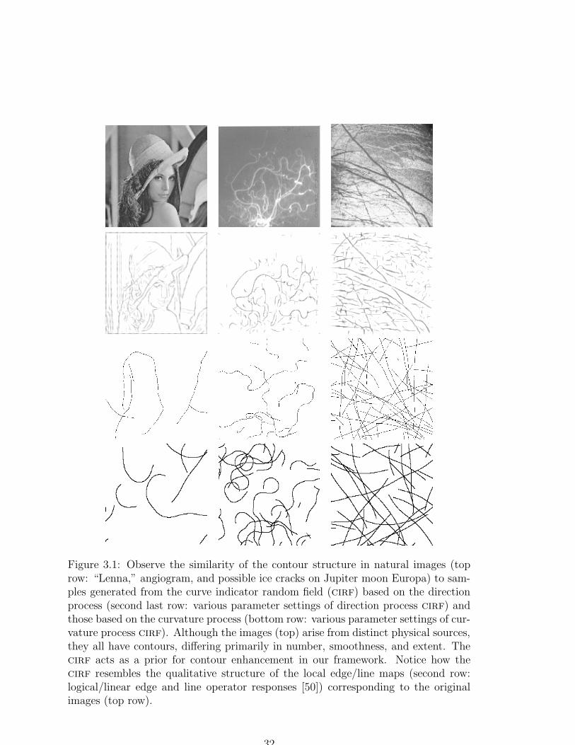
Figure 3.1: Observe the similarity of the contour structure in natural images (toprow: “Lenna,” angiogram, and possible ice cracks on Jupiter moon Europa) to sam-ples generated from the curve indicator random field (cirf) based on the directionprocess (second last row: various parameter settings of direction process cirf) andthose based on the curvature process (bottom row: various parameter settings of cur-vature process cirf). Although the images (top) arise from distinct physical sources,they all have contours, differing primarily in number, smoothness, and extent. Thecirf acts as a prior for contour enhancement in our framework. Notice how thecirf resembles the qualitative structure of the local edge/line maps (second row:logical/linear edge and line operator responses [50]) corresponding to the originalimages (top row).

32

Thus Ui is the total amount of time that all of the Markov processes spent in site i.

Again, observe that this definition satisfies the desiderata for an ideal edge/line map

suggested in Chapter 1: (1) non-zero valued where the contours are, and (2) zero-

valued elsewhere. We emphasize that the curve indicator random field is a different

object than the curves used to produce it. First, the cirf describes a random set

of curves; each one is a Markov process. Second, and more importantly, the cirf

is a stochastic function of space, i.e., a random field, whereas each (parameterized)

curve is a random function of time. This transformation from a set of random curves

to a random field makes the cirf an idealization of local edge/line responses, and

sets the stage for contour enhancement where the probability distribution of U will

become our prior for inference. See Fig. 3.1 for some samples generated by the cirf

prior.

3.1.1 Global to Local: Contour Intersections and the CIRF

In addition to representing the loss of contour parameterization, the cirf locally

captures the global contour properties of intersection and self-intersection (§2.1.1).

This fact has nothing to do with the particular contour distributions used (Marko-

vianity and independence, for example); it is a consequence of the cirf definition.

A measure of self-intersection, or the lack of simplicity of a contour, is the square of

the single-curve cirf, or

V 2i =

(∫ Rt = i dt

)(∫ Rt′ = i dt

)=

∫ (∫ Rt′ = Rt = i dt′

)dt.

To understand why V 2i measures self-intersection, consider the expression in paren-

theses on the right: if the process R was in site i at time t, then this expression

counts the total amount of time spent in site i = Rt; otherwise it is zero. There are

33

two components to this time: (1) the (unavoidable) holding time of Rt in site i (i.e.,

how much time spent in i for the visit including time t) and (2) the remainder, which

evidently must be the time spent in site i before or after the visit that included time

t, i.e., the self-intersection time of Rt = i. Taking the integral over t, we therefore see

that V 2i is a measure of self-intersection for site i over the entire contour. In continu-

ous space and for Brownian motion, Dynkin has studied such self-intersection times

by considering powers of local times for quantum field theory (which is essentially the

single-curve cirf where the indicator is replaced with a Dirac δ-distribution) [24].

A similar calculation can be carried out for the multiple-curve case U 2i , where

we will get terms with integrals over the same curve as above (to measure self-

intersection), or over a pair of distinct curves where instead we get an analogous

intersection or crossing measure. The key is to recognize that a global contour

property that requires checking the entire parameterization—intersection—becomes

a local property (squaring) of the cirf. If desired, we could exploit this property

to enforce non-intersecting curves by penalizing non-zero values of the square of the

cirf. This would amount to changing our prior to one without our assumed indepen-

dence among curves, for example. Instead of taking that direction, we first explore

what statistical structure can be tractably captured without including intersections.

Somewhat surprisingly however, we shall see later (§5.2) that the square of the cirf

will re-emerge in the likelihood (noise and observation model), penalizing contour

intersections automatically.

3.2 Moments of the Single-Curve CIRF

Probabilistic models in vision and pattern recognition have been specified in a num-

ber of ways. For example, Markov random field models [36] are specified via clique

34

potentials and Gaussian models are specified via means and covariances. Here, in-

stead of providing the distribution of the curve indicator random field itself, we derive

its moment generating functional, from which all moments are then computed.

Although we are interested in the statistics of the general curve indicator random

field U , we first consider the simpler, single-curve case, which we studied earlier

in discrete-time [4]. The first step (Prop. 1) is to derive all the moments of the

single-curve cirf V . Then we shall summarize this result as a moment generating

functional (Prop. 2).

To prepare for studying these moments, we first recognize the rather pathological

nature of the cirf: realizations of this field are zero except along the curves. While

we do not develop this connection here, we observe that when the state space is a con-

tinuum, realizations of the analogous1 cirf would generally not even be continuous;

hence we would be faced with generalized functions, or distributions (in the sense of

Schwartz, not probability), where the field is probed by taking inner products with

(appropriately well-behaved) “test functions” [99].

It is also convenient to use this distribution-theoretic formalism for studying the

cirf on our discrete space I. To do so, we first define the inner product 〈a, b〉 :=

∑i∈I aibi. We use a bias vector c ∈ |I| to act as a “probe” or “test function”

function on V by taking an inner product:

〈c, V 〉 =∑

i

ci

∫ Rt = idt =

∫ (∑

i

ci Rt = i

)dt =

∫c(Rt)dt, (3.1)

where c(i) = ci. The integral∫c(Rt)dt is known as an additive functional of Markov

process Rt [30]. In the following, we let α := λ−1 to simplify expressions. We also

introduce a final weighting ν(RT−) on the state of the curve just before death; ν can

1Loosely, we obtain cirf in the continuum by replacing the indicators above with Dirac δ-distributions [3].

35

be used to encourage the curve to end in certain states over others.2 Let

iZ denote

the expected value of the random variable Z given that R0 = i, and let

µZ denote

the same expectation except given that R0 = i = µi, where µ is the distribution

of the initial point of the curve. To reduce the clutter of many brackets we adopt

the convention that the expectation operator applies to all multiplied (functions of)

random variables to its right: e.g.,f(X)g(Y ) :=

[f(X)g(Y )]. We now provide a

formula for the moments of 〈c, V 〉, a “probed” single-curve cirf V . The proof uses

techniques that are used in statistical physics and in studying order-statistics.

Proposition 1. The k-th moment of 〈c, V 〉 with initial distribution µ and final

weighting ν = ν(i) = νi, i ∈ I is:

µ〈c, V 〉kν(RT−) = αk!〈µ, (GC)kGν〉, (3.2)

where C = diag c.

proof. We first consider the case where µj = δi,j, and then generalize. Recall the

formula for exponentially-distributed length T : pT (t) = α e−αt . Substituting this and

(3.1) into the left side of (3.2), we get:

i〈c, V 〉kν(RT−) =

i

(∫ T

0

c(Rt)dt

)k

ν(RT−)

= α

i

∫ ∞

0

e−αt

(∫ t

0

c(Rt′)dt′

)k

ν(Rt)dt, (3.3)

where we have used the fact that:

∫f(t−)dt =

∫f(t)dt,

2Following [30], we use the notation T− to represent the left limit approaching T from below,i.e., ν(RT−) = limtT ν(Rt).

36

for piecewise continuous functions f with finite numbers of discontinuities in finite

intervals. We further note that:

(∫ t

0

c(Rt′)dt′

)k

=

∫ t

0

· · ·∫ t

0

c(Rt1) · · · c(Rtk)dt1 · · ·dtk

= k!

∫· · ·∫

0≤t1≤···≤tk≤t

c(Rt1) · · · c(Rtk)dt1 · · ·dtk, (3.4)

where the second line follows because there are k! orthants in the k-dimensional cube

[0, t]k, each having the same integral by relabeling the ti’s appropriately. Taking

integrals iteratively starting with respect to t1, the right side of (3.4) becomes, by

induction in k:

k!

∫ t

0

∫ tk

0

· · ·∫ t2

0

c(Rt1) · · · c(Rtk)dt1 · · ·dtk.

The right side of (3.3) then becomes:

αk!

∫ ∞

0

e−αt

∫ t

0

∫ tk

0

· · ·∫ t2

0

∑

i1,...,ik,j

iRt1 = i1, . . . , Rtk = ik, Rt = j

· c(i1) · · · c(ik)ν(j)dt1 · · ·dtk

= αk!∑

i1,...,ik,j

c(i1) · · · c(ik)ν(j)[∫ ∞

0

e−αt

·∫ t

0

∫ tk

0

· · ·∫ t2

0

pi,i1(t1)pi1,i2(t2 − t1)

· · ·pik−1,ik(tk − tk−1)pik ,j(t− tk)dt1dt2 · · ·dtk−1

dtk

], (3.5)

37

using the Markovianity and stationarity of Rt. Recalling that the formula for the

convolution of two functions f and g is:

(f ∗ g)(t) =

∫ t

0

f(τ)g(t− τ)dτ,

we see that the expression in braces in (3.5) can be written as:

∫ t

0

· · ·∫ t2

0

pi,i1(t1)pi1,i2(t2 − t1)dt1 · · ·pik,j(t− tk)dtk−1

=

∫ t

0

· · ·∫ t3

0

(pi,i1 ∗ pi1,i2)(t2)pi2,i3(t3 − t2)dt2 · · · pik,j(t− tk)dtk−1

= (pi,i1 ∗ pi1,i2 ∗ · · · pik−1,ik ∗ pik,j)(t),

which is a k-fold convolution by induction in k. Now observe that the expression in

brackets in (3.5) is the Laplace transform h(t)(α) with respect to t, evaluated at

α, of the expression h(t) in braces. Therefore by using the convolution rule of the

Laplace transform k times, the expression in brackets in (3.5) becomes:

pi,i1(α) · pi1,i2(α) · · · · · pik−1,ik(α) · pik,j(α).

38

But as shown earlier we know that gi,j =∫∞0

e−αt pi,j(t)dt = pi,j(α), and so we

can write:

i〈c, V 〉kν(RT−)

= αk!∑

i1,...,ik,j

c(i1) · · · c(ik)ν(j)gi,i1gi1,i2 · · · gik−1,ikgik,j (3.6)

= αk!∑

i1

gi,i1c(i1)

∑

i2

gi1,i2c(i2) · · ·[∑

ik

gik−1,ikc(ik)

(∑

j

gik,jν(j)

)]· · ·

= αk!∑

i1

(GC)i,i1

∑

i2

(GC)i1,i2 · · ·[∑

ik

(GC)ik−1,ik(Gν)ik

]· · ·

= αk!((GC)kGν)i.

Since for any random variable Z we have

µZ =∑

i

R0 = i [Z|R0 = i] =

∑i µi

iZ, the result follows.

3.3 Moment Generating Functional of the

Single-Curve CIRF: A Feynman-Kac Formula

To obtain a formula for the moment generating functional (mgf) of the single-curve

cirf, we first define the Green’s operator G(c) = Gc with (spatially-varying) bias

(vector) c as the Green’s operator for the killed Markov process with extra killing

−c, i.e., having generator Q(c) := Q + C, where C = diag(c1, . . . , c|I|). The bias c

behaves exactly opposite to the decay or death term α in Q = L−αI: if ci is positive,

there is a bias towards the creation of particles at site i; if negative, there is a bias

towards killing them. Using an argument similar to the proof of Lemma 1, we know

G(c) := −Q(c)−1 = −(Q+C)−1. We provide an explicit condition for the invertibility

39

of Q+C later (Prop. 3). We now compute the moment generating functional for the

single-curve case using Prop. 1. This is known as the Feynman-Kac formula [22].

Proposition 2. For all c ∈ |I| such that |c| is sufficiently small,

µ exp〈c, V 〉ν(RT−) = α〈µ,G(c)ν〉.

proof. Using the power series representation of the exponential, we write:

µ exp〈c, V 〉ν(RT−) =

µ

∞∑

k=0

〈c, V 〉kk!

ν(RT−)

=∞∑

k=0

µ〈c, V 〉kν(RT−)/k! =

∞∑

k=0

α〈µ, (GC)kGν)〉 (3.7)

using Prop. 1. Recalling the fact that∑∞

k=0Ak = (I−A)−1, as long as ||A|| < 1, the

right hand side of (3.7) becomes:

α〈µ,[

∞∑

k=0

(GC)k

]Gν〉 = α〈µ, (I −GC)−1Gν〉,

as long as (for some operator norm) ||GC|| < 1. Since C = diag(c1, . . . , c|I|) is

diagonal, the matrix GC is simply G with the i-th column weighted by ci. Therefore

||GC|| < 1 for |c| sufficiently small. The result follows because (I − GC)−1 =

(Q−1Q+Q−1C)−1 = −(Q + C)−1G−1.

Observe that to evaluate the Feynman-Kac formula, one must solve the linear

system (Q + C)h + ν = 0 for h. This equation will become a key component in the

filters of Chapter 5; numerical methods are described in §6.1 and §6.2.

40

3.3.1 Sufficient Condition For MGF Convergence:

Khas’minskii’s Condition

The proof of Prop. 2 suggests with the following condition, first studied by Khas’-

minskii [57], for the convergence of the Feynman-Kac formula.

Proposition 3. The moment generating functional of the (single-curve) curve indi-

cator random field V converges if ||G|c| ||∞ < 1.

proof. Using the ∞-norm, we consider the convergence condition in the proof of

Prop. 2:

1 > ||GC||∞ = supi

∑

j

|(GC)i,j| = supi

(G|C|1)i = supi

(G|c|)i,

where 1 = (1, . . . , 1) and using the facts that G has positive entries and operator C

is diagonal.

The Khas’minskii condition is easy to check: one just takes the componentwise

absolute value of c (which later will be an input), and then “blur” it with the Green’s

operator G. If any component of the result is greater than 1, the moment generating

functional may not converge. As we shall see in §6.2, this condition will be exploited

in our numerical methods for filtering.

3.3.2 Initial and Final Weightings

As the interpretation of the “final weighting” ν above may seem mysterious, we

now restrict µ and ν to be finite measures satisfying the normalization constraint

1 = 〈µ,Gν〉. (If this equality is not satisfied, one need only divide by a suitable

normalizing constant.)

41

Corollary 1. Suppose that the joint distribution over initial and final positions is

R0 = i, RT− = j = µigi,jνj. Then the moment generating functional of V , with

this joint distribution over initial and final states, is:

exp〈c, V 〉 = 〈µ,G(c)ν〉. (3.8)

Remark 1. Although not studied here, it is interesting to consider the problem

of finding those measures µ, ν that induce a R0, RT− with prescribed marginals

R0 and RT− over initial and final states respectively.

Since we are most interested in the case where µ and ν are spatially constant, we

can forego answering this question now. Before we begin the proof of this corollary,

we state a basic result.

Lemma 2. If X and Z are random variables, and X is discrete (i.e., X can only

take on one of an at most countable number of values x), then:

[Z|X = x] =

Z

X = x X = x .

proof. We compute:

[Z|X = x] =

∫z

Z ∈ dz|X = x =

∫z

Z ∈ dz,X = x/ X = x

=

∫ ∑

x′

z x′ = x Z ∈ dz,X = x′/ X = x =

Z

X = x/ X = x.

42

proof of corollary 1. Observe that µigi,jνj is indeed a distribution. We now

compute the result:

exp〈c, V 〉 =

∑

i,j

R0 = i, RT− = j [exp〈c, V 〉|R0 = i, RT− = j]

=∑

i,j

µigi,jνj

i[exp〈c, V 〉|RT− = j]

=∑

i,j

µigi,jνj

i[exp〈c, V 〉 RT− = j]/

iRT− = j,

using Lemma 2. But using Prop. 2 we see that:

iRT− = j =

i exp(0, V )

RT− = j = αgi,j,

and therefore:

exp〈c, V 〉 = α−1

∑

i,j

µiνj

i[exp〈c, V 〉 RT− = j]

= α−1 µ

[exp〈c, V 〉

(∑

j

νj RT− = j

)]

= α−1 µ [exp〈c, V 〉ν(RT−)] .

The result follows after another application of Prop. 2 to the above expectation.

The next corollary shows all of the (joint) moments of V . Let permk denote the

set of permutations of the integers 1, . . . , k.

Corollary 2. If k ≥ 1, the k-th (joint) moment of V at sites i1, . . . , ik is:

Vi1 · · ·Vik =

∑

i,j

µiνj

∑

a∈permk

giia1gia1 ia2

· · · giak−1iakgiak

j. (3.9)

43

proof. Take partial derivatives of (3.8) with respect to ci1 , . . . , cik and evaluate

them at c = 0. The only nonzero terms come from differentiating an expression

proportional to (3.6).

In our earlier work on the curve indicator random field for discrete-time Markov

processes [4], we arrived at a similar result, except under the condition that the sites

i1, . . . , ik are distinct. In observing the connection to the Feynman-Kac formula, we

have overcome this limitation and can now summarize the single-curve cirf with its

moment generating functional. The weighting over final states (the other end of the

contour) is also new.

3.4 Multiple-Curve Moment Generating Functional

In order to model more than one curve in an image, we need a joint distribution

over both the number of curves and the curves (and the corresponding cirfs) them-

selves. To make our computations concrete, we adopt a Poisson distribution over

the number N of curves, and assume conditional independence of the curves given

N . To compute the moment generating functional of this (multiple-curve) cirf as

a Poisson distribution over (single-curve) cirfs, we first consider the general case

of Poisson “point” process given a distribution over each point, where point will be

interpreted as an entire single-curve cirf.

3.4.1 The Poisson Measure Construction

We begin with a finite measure3 P : F → + over the measure space (Ω,F), where

F is a σ-algebra, and

+ denotes the nonnegative real numbers. Intuitively, the

3A finite measure can always be normalized to a probability distribution because P (Ω) < ∞. Inparticular, P (ω) := P (ω)/P (Ω) is a (normalized) probability distribution over ω.

44

finite measure P is the (un-normalized) distribution over “points” ω ∈ Ω, where

in this thesis ω is a curve realization (i.e., a Markov process realization) and Ω is

the set of all possible curves. We shall now define a probability distribution over

random configurations ω = (ω1, ..., ωN ) ∈ Con(Ω) := Ω0 =, Ω1 = Ω, Ω2 =

Ω × Ω, Ω3, . . ., where each ωn is a curve in Ω and N is the random number of

curves. In our context, Ω0 is the 0-curve configuration (no curves), Ω1 are the one-

curve configurations (the set of single curves), Ω2 are the two-curve configurations

(the set of pairs of curves), and so on. We now compute the Poisson point measure

via its expectationF on any (measurable) function F : Con(Ω) →

(clearly

this defines a probability distribution for we could take F as an indicator over any

(measurable) subset of Con(Ω) to get its probability).

Proposition 4. Suppose N is a Poisson deviate with mean P (Ω). Further suppose

that the points ω1, . . . , ωn are (conditionally) independent and identically distributed

with P (·)/P (Ω), given N = n. Then:

F :=

∞∑

n=0

e−P (Ω)

n!

∫

Ωn

F (ω1, . . . , ωn)P (dω1) · · ·P (dωn). (3.10)

proof. We need only take a conditional expectation and recall the formula for the

Poisson distribution, as follows:

F =

(

[F |N ])

=(

F (ω1, . . . , ωN ))

=(∫

ΩN

F (ω1, . . . , ωN ) (P (dω1)/P (Ω)) · · · (P (dωN )/P (Ω))

)

=∞∑

n=0

e−P (Ω) P (Ω)n

n!

(P (Ω)−n

∫

ΩN

F (ω1, . . . , ωN )P (dω1) · · ·P (dωN )

).

The result follows.

45

The above presentation of the Poisson point measure is based on Dynkin [22].

3.4.2 Application to the MGF of the Curve Indicator

Random Field for Multiple Curves

We now finally consider the joint distribution over many curves. Suppose there are

N contours on average, and that µ and ν are finite measures on I (vectors in |I|),

characterizing the initial and final positions, respectively, of the Markov processes

R(n)t : n = 1, . . . ,N. As before, these measures satisfy the normalization constraint

〈µ,Gν〉 = 1. For general-purpose contour enhancement, we typically have no a-priori

preference for the start and end locations of each contour, and so we would set these

measures proportional to the constant vector 1 = (1, . . . , 1). One can show that by

letting µi = |I|−1, νi = λ−1, ∀i ∈ I, the above constraint is satisfied. We now state

and prove the key theoretical result of this thesis, which is most closely related to

the work by Dynkin [22].

Proposition 5. Suppose the inital distribution µ and final weighting ν satisfy the

normalization constraint 〈µ,Gν〉 = 1. Then the moment generating functional of the

curve indicator random field U is

exp〈c, U〉 = exp〈µ, N (G(c)−G)ν〉.

proof. To take advantage of the Poisson point measure construction, we let ω be a

realization of the killed Markov process Rt, t ∈ [0, T−), such that the finite measure

P = P (ω) is the probability distribution for ω but multiplied by the constant N ,

i.e., P (Ω) = N . Let F := exp〈c, U〉 = exp∑N

n=0〈c, V (n)〉 =∏N

n=0 exp〈c, V (n)〉, where

46

V (n) is a function of ωn. Applying (3.10) we obtain:

exp〈c, U〉 =

∞∑

n′=0

e−P (Ω)

n′!

∫

Ωn′

n′∏

n=0

exp〈c, V (n)〉P (dω1) · · ·P (dωn′)

=

∞∑

n′=0

e−P (Ω)

n′!

n′∏

n=0

(∫

Ω

exp〈c, V (n)〉P (dωn)

)

= e−P (Ω)

∞∑

n′=0

1

n′!

n′∏

n=0

(∫

Ω

exp〈c, V (1)〉P (dω1)

),

since V (1), . . . , V (n′) are identically distributed. But then the latter integral is N exp〈c, V 〉,

and so the above sum becomes:

∞∑

n′=0

(N

exp〈c, V 〉)n′

/n′! = exp(N exp〈c, V 〉).

So using P (Ω) = N 〈µ,G(0〉ν) and Prop. 1, we conclude:

exp〈c, U〉 = exp(N 〈µ,G(c)ν〉 − N 〈µ,Gν〉).

3.4.3 Cumulants of the CIRF

While Prop. 5 may seem abstract, it is actually very useful. First observe that how

similar in form it is to the single-curve case. More importantly, with Prop. 5 we can

compute the higher-order cumulants [66, 84] of U (recall that the moments define

the cumulants and vice versa):

47

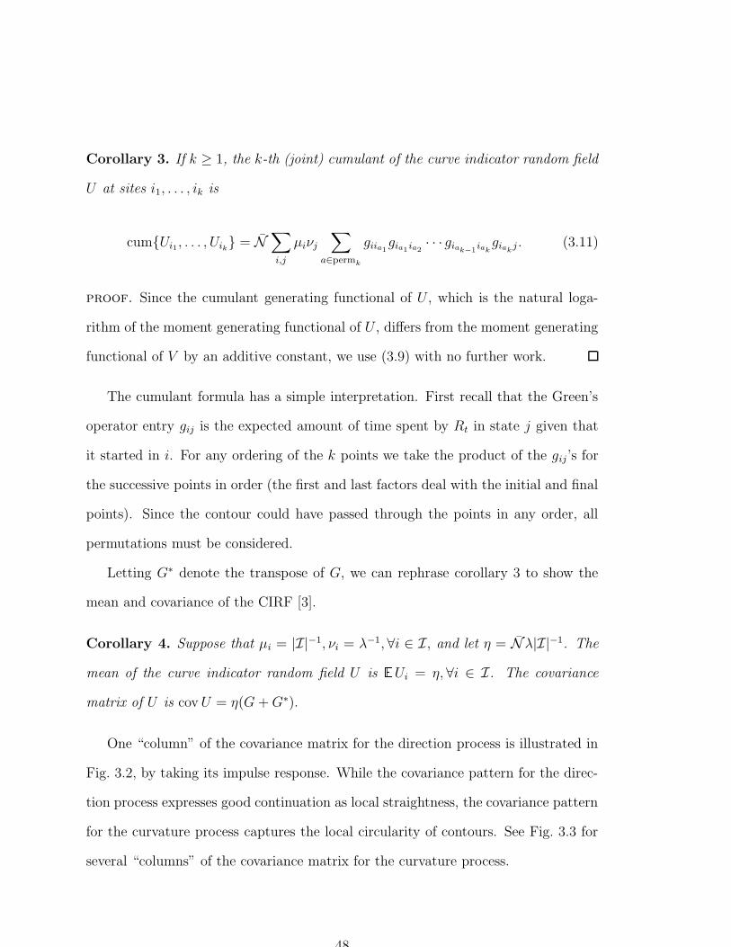
Corollary 3. If k ≥ 1, the k-th (joint) cumulant of the curve indicator random field

U at sites i1, . . . , ik is

cumUi1, . . . , Uik = N∑

i,j

µiνj

∑

a∈permk

giia1gia1 ia2

· · · giak−1iakgiak

j. (3.11)

proof. Since the cumulant generating functional of U , which is the natural loga-

rithm of the moment generating functional of U , differs from the moment generating

functional of V by an additive constant, we use (3.9) with no further work.

The cumulant formula has a simple interpretation. First recall that the Green’s

operator entry gij is the expected amount of time spent by Rt in state j given that

it started in i. For any ordering of the k points we take the product of the gij’s for

the successive points in order (the first and last factors deal with the initial and final

points). Since the contour could have passed through the points in any order, all

permutations must be considered.

Letting G∗ denote the transpose of G, we can rephrase corollary 3 to show the

mean and covariance of the CIRF [3].

Corollary 4. Suppose that µi = |I|−1, νi = λ−1, ∀i ∈ I, and let η = Nλ|I|−1. The

mean of the curve indicator random field U isUi = η, ∀i ∈ I. The covariance

matrix of U is covU = η(G+G∗).

One “column” of the covariance matrix for the direction process is illustrated in

Fig. 3.2, by taking its impulse response. While the covariance pattern for the direc-

tion process expresses good continuation as local straightness, the covariance pattern

for the curvature process captures the local circularity of contours. See Fig. 3.3 for

several “columns” of the covariance matrix for the curvature process.

48

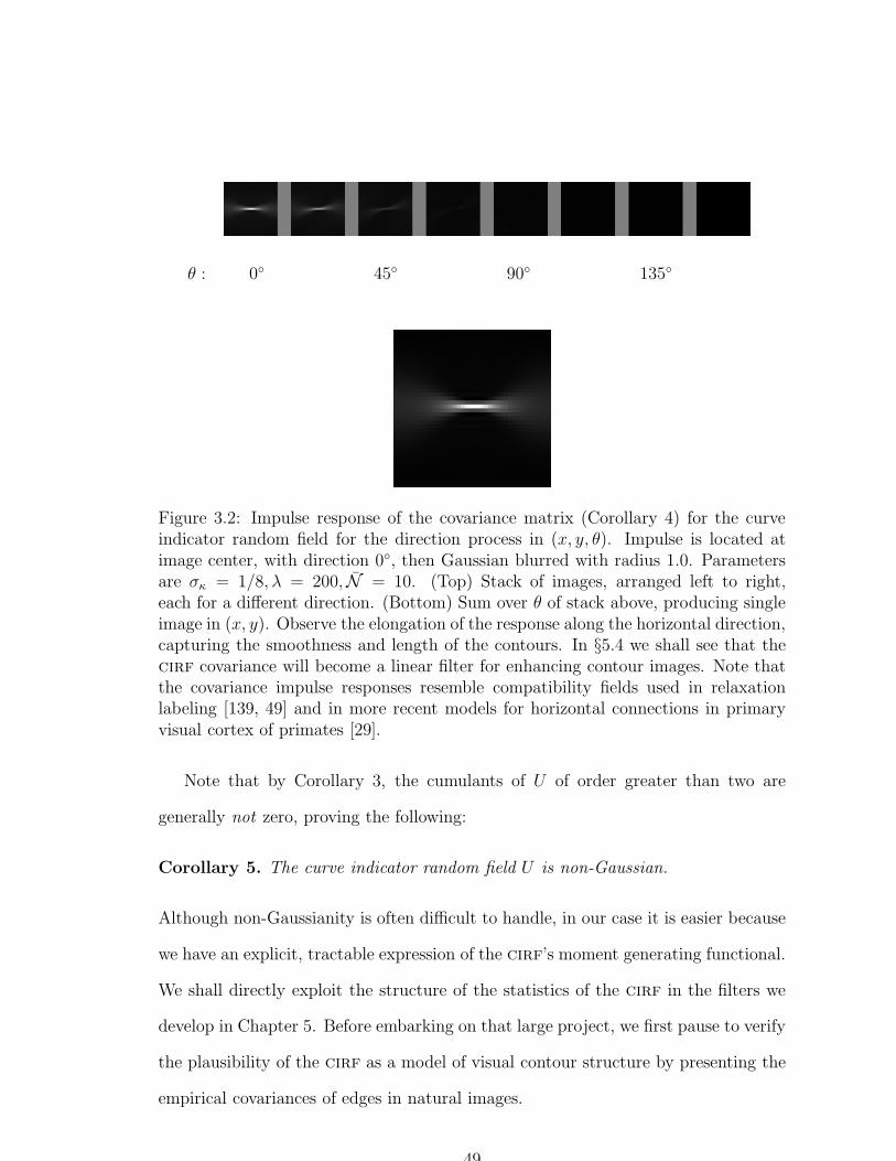
θ : 0 45 90 135

Figure 3.2: Impulse response of the covariance matrix (Corollary 4) for the curveindicator random field for the direction process in (x, y, θ). Impulse is located atimage center, with direction 0, then Gaussian blurred with radius 1.0. Parametersare σκ = 1/8, λ = 200, N = 10. (Top) Stack of images, arranged left to right,each for a different direction. (Bottom) Sum over θ of stack above, producing singleimage in (x, y). Observe the elongation of the response along the horizontal direction,capturing the smoothness and length of the contours. In §5.4 we shall see that thecirf covariance will become a linear filter for enhancing contour images. Note thatthe covariance impulse responses resemble compatibility fields used in relaxationlabeling [139, 49] and in more recent models for horizontal connections in primaryvisual cortex of primates [29].

Note that by Corollary 3, the cumulants of U of order greater than two are

generally not zero, proving the following:

Corollary 5. The curve indicator random field U is non-Gaussian.

Although non-Gaussianity is often difficult to handle, in our case it is easier because

we have an explicit, tractable expression of the cirf’s moment generating functional.

We shall directly exploit the structure of the statistics of the cirf in the filters we

develop in Chapter 5. Before embarking on that large project, we first pause to verify

the plausibility of the cirf as a model of visual contour structure by presenting the

empirical covariances of edges in natural images.

49

κ0: 0.2 0 -0.1

Figure 3.3: Impulse responses of the covariance matrix for the curve indicator randomfield for the curvature process. Impulses are located at the center of each image,directed at discrete direction 4 out of 32, with 5 curvatures. Parameters are σκ =0.01, λ = 10. Each pixel represents an integral over all directions and curvaturesassociated with that position; the actual impulse response in each case is a sparse4-dimensional array.

50

Chapter 4

Edge Correlations

in Natural Images

Whether an algorithm ever works depends on the correctness of the assumptions

upon which it is based. It is therefore useful to determine if the cirf model of

contours bears any resemblance to natural contour images so that our efforts are

not wasted on an unrealistic model. Last chapter we derived the covariances of the

cirf U ; here we present empirical edge covariances for several natural images. The

qualitative similarity between the covariances for our model and the observations

suggests that the cirf based on the direction process is a reasonable starting point

for modeling image contours; the results also suggest a role for the curvature process.

Although we cannot measure the covariances of U directly (since we cannot ob-

serve its realizations), we can estimate covariances in local edge operator responses,

or what we shall the measurement field M . These correlations1 can reveal, albeit

crudely, the qualitative structure of the correlations of U .

1Following common practice, the terms correlation and covariance will be used interchangeablyunless there is confusion.

51

While a detailed treatment of observation models will be presented in Chap-

ter 5, we briefly mention the connection between the covariances ΣM and ΣU , of M

and U , respectively. Suppose that the measurement field M was generated by the

corruption of the cirf U with blur operator B with additive noise N , statistically

independent of U . Because of the independence of N , the cumulant generating func-

tional of the measurements M = BU + N is the sum of the cumulant generating

functions for BU and N respectively. This implies that the measurement covariance

is ΣM = ΣBU + ΣN = BΣUB∗ + ΣN , where B∗ is the transpose of B. If the noise

is relatively white and the blur has relatively small scale, then this result says that

the measurement covariances will be a slightly blurry form of the cirf covariances,

but different along the diagonal. Therefore studying the measurement covariances is

warranted for verifying the plausibility of the cirf.

To carry out our observations, we use oriented edge filter banks. Specifically,

at each image position (x, y) and direction θ we shall measure the edge strength

m(x, y, θ), which is a realization of the random variable M(x, y, θ).2 The resultant

set of these random variables forms our measurement random field M = M(·). The

analysis in the previous paragraph suggests that for good continuation to have any

meaning for natural contour images, at least the following must hold:

Conjecture 1. For natural images, M is not “white,” i.e., its covariance

ΣM (r1, r2) := E[(M(r1)− E[M(r1)])(M(r2)− E[M(r2)])] 6= 0,

for all r1 6= r2, where ri := (xi, yi, θi).

2In this chapter we are using explicit spatial coordinates instead of the abstract site index i.

52

In §4.2, we shall present direct evidence not only in support of this conjecture, but

also in agreement with the cirf model: the observed edge correlations have an

elongated pattern.

After first presenting the results in this chapter [5], we found a paper by Oka-

jima [88] in which edge correlations of natural images were observed and used for

learning edge filters. After publishing our work [3], we found that Kruger [64] and

Schaaf [123] had already independently observed an elongated structure in edge cor-

relations as well. This research area has recently become very active, with edge

correlation reports in [34] and [110]. One distinction of our work is that we assume

the statistical homogeneity (§4.1) that is qualitatively apparent in others’ results,

allowing us to compute edge correlations from a single image. This suggests that it

is possible to adapt or “tune” contour filter parameters to individual images. A more

important difference is the theoretical cirf framework we provide for interpreting

these observations.

More generally, Elder and Krupnik have recently estimated the statistical power

of grouping cues other than good continuation [25]. Martin et al have computed

statistics of Gestalt cues as well, but using hand-segmented images instead [74]. In

related work on image statistics, the joint distributions of neighboring wavelet coef-

ficients have been measured [111, 44]. Mumford and Gidas have recently suggested

an axiomatic generative model of natural images using infinitely divisible distribu-

tions [83]. We currently ignore higher-order moments in order to focus on the longer

distance spatial variation of edge relations. Invoking techniques from the study of tur-

bulence, self-similarity properties in image gradients have also been measured [120].

For a review of natural images statistics, see [104].

53

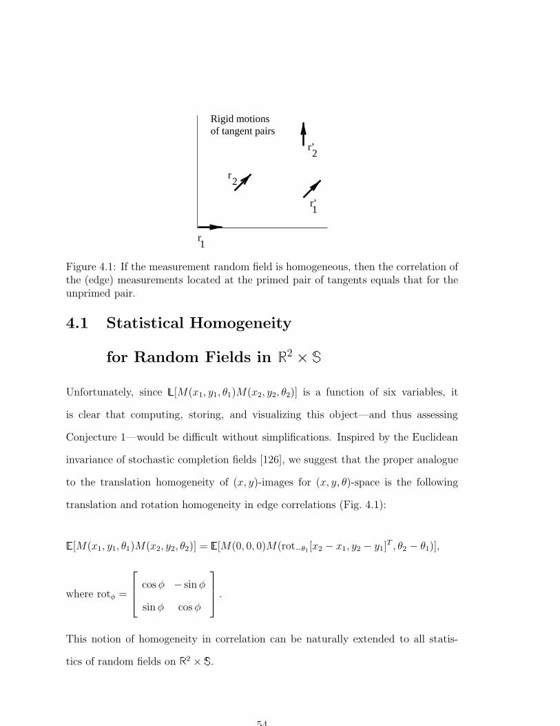
Rigid motionsof tangent pairs

r’

r1

2r

1r’

2

Figure 4.1: If the measurement random field is homogeneous, then the correlation ofthe (edge) measurements located at the primed pair of tangents equals that for theunprimed pair.

4.1 Statistical Homogeneity

for Random Fields in 2 ×

Unfortunately, since [M(x1, y1, θ1)M(x2, y2, θ2)] is a function of six variables, it

is clear that computing, storing, and visualizing this object—and thus assessing

Conjecture 1—would be difficult without simplifications. Inspired by the Euclidean

invariance of stochastic completion fields [126], we suggest that the proper analogue

to the translation homogeneity of (x, y)-images for (x, y, θ)-space is the following

translation and rotation homogeneity in edge correlations (Fig. 4.1):

[M(x1, y1, θ1)M(x2, y2, θ2)] = [M(0, 0, 0)M(rot−θ1 [x2 − x1, y2 − y1]T , θ2 − θ1)],

where rotφ =

cosφ − sinφ

sinφ cos φ

.

This notion of homogeneity in correlation can be naturally extended to all statis-

tics of random fields on 2 × .

54

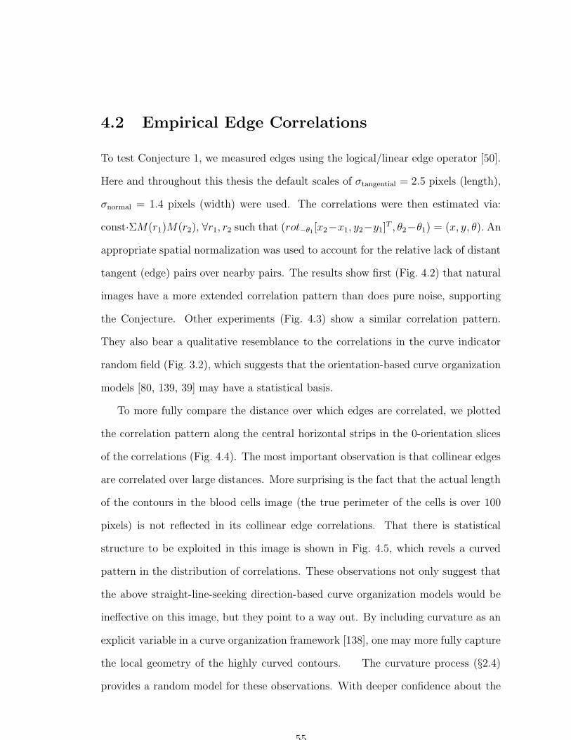
4.2 Empirical Edge Correlations

To test Conjecture 1, we measured edges using the logical/linear edge operator [50].

Here and throughout this thesis the default scales of σtangential = 2.5 pixels (length),

σnormal = 1.4 pixels (width) were used. The correlations were then estimated via:

const·ΣM(r1)M(r2), ∀r1, r2 such that (rot−θ1[x2−x1, y2−y1]T , θ2−θ1) = (x, y, θ). An

appropriate spatial normalization was used to account for the relative lack of distant

tangent (edge) pairs over nearby pairs. The results show first (Fig. 4.2) that natural

images have a more extended correlation pattern than does pure noise, supporting

the Conjecture. Other experiments (Fig. 4.3) show a similar correlation pattern.

They also bear a qualitative resemblance to the correlations in the curve indicator

random field (Fig. 3.2), which suggests that the orientation-based curve organization

models [80, 139, 39] may have a statistical basis.

To more fully compare the distance over which edges are correlated, we plotted

the correlation pattern along the central horizontal strips in the 0-orientation slices

of the correlations (Fig. 4.4). The most important observation is that collinear edges

are correlated over large distances. More surprising is the fact that the actual length

of the contours in the blood cells image (the true perimeter of the cells is over 100

pixels) is not reflected in its collinear edge correlations. That there is statistical

structure to be exploited in this image is shown in Fig. 4.5, which revels a curved

pattern in the distribution of correlations. These observations not only suggest that

the above straight-line-seeking direction-based curve organization models would be

ineffective on this image, but they point to a way out. By including curvature as an

explicit variable in a curve organization framework [138], one may more fully capture

the local geometry of the highly curved contours. The curvature process (§2.4)

provides a random model for these observations. With deeper confidence about the

55

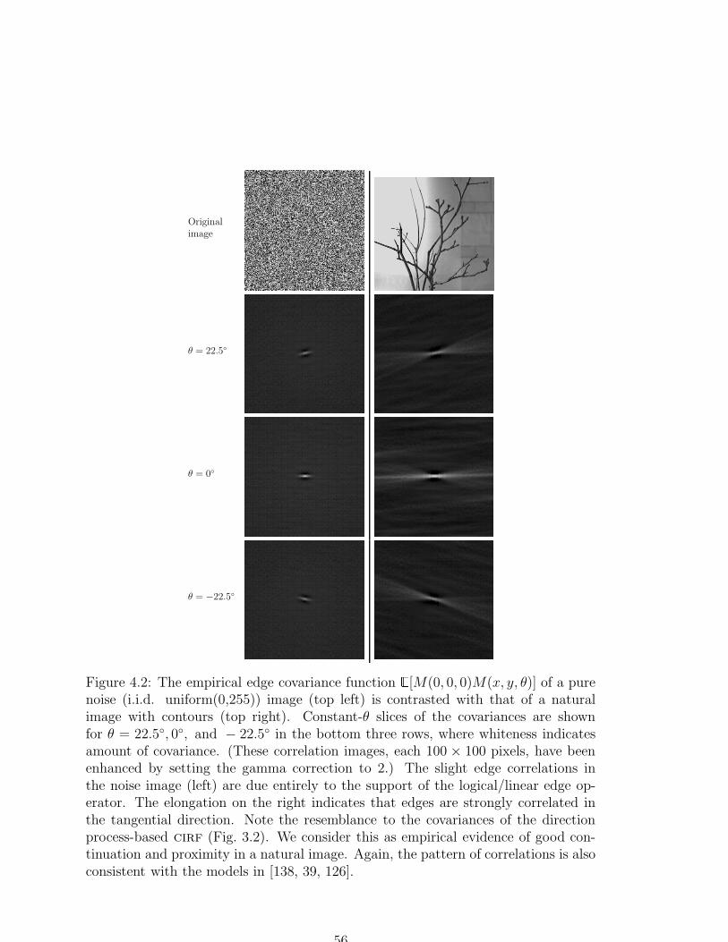
Originalimage

θ = 22.5

θ = 0

θ = −22.5

Figure 4.2: The empirical edge covariance function[M(0, 0, 0)M(x, y, θ)] of a pure

noise (i.i.d. uniform(0,255)) image (top left) is contrasted with that of a naturalimage with contours (top right). Constant-θ slices of the covariances are shownfor θ = 22.5, 0, and − 22.5 in the bottom three rows, where whiteness indicatesamount of covariance. (These correlation images, each 100 × 100 pixels, have beenenhanced by setting the gamma correction to 2.) The slight edge correlations inthe noise image (left) are due entirely to the support of the logical/linear edge op-erator. The elongation on the right indicates that edges are strongly correlated inthe tangential direction. Note the resemblance to the covariances of the directionprocess-based cirf (Fig. 3.2). We consider this as empirical evidence of good con-tinuation and proximity in a natural image. Again, the pattern of correlations is alsoconsistent with the models in [138, 39, 126].

56

Figure 4.3: Edge covariances (continued; see caption of Fig. 4.2 for explanation).The Paolina (left) and lily (center) images have correlations in the tangential direc-tion which extend much farther than those for the blood cells image (right). Notehow these more distant correlations in the Paolina image occur despite the contoursbeing open, unlike the closed contours in the blood cell image, suggesting curveenhancement systems should not rely only on contour closure.

57

0.01

0.1

1

5 10 15 20 25 30 35 40 45 50

Distance [pixels]

Correlation of Collinear Edges

TwigsPaolina

LilyBlood cells

Noise

Figure 4.4: Comparison of the correlation coefficient between collinear edges, ob-tained by extracting a central strip

M(0, 0, 0)M(x, 0, 0) through the zero-orientation

slices of the correlations in Figs. 4.2 and 4.3, subtracting the square of the mean(estimated by taking a spatial average in an approximately constant region of thecovariance), and then dividing by the estimated variance of M . Observe that al-though the correlation of a pure noise image falls off rapidly, the correlation fornatural images persists over much longer distances. For example, note that even at25 pixels of separation, collinear edges in the twigs (Fig. 4.2, right), Paolina and lily(Fig. 4.3, left and center) images are appreciably more correlated than pure noise.The correlation of the blood cells image drops off rapidly due to high curvature (seeFig. 4.5).

relevance of the cirf to real images, we now turn to the task of deriving contour

enhancement filters.

58

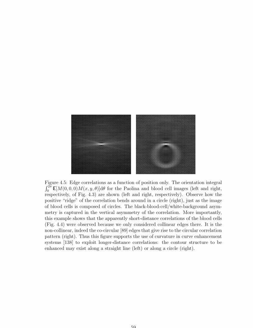
Figure 4.5: Edge correlations as a function of position only. The orientation integral∫ 2π

0

[M(0, 0, 0)M(x, y, θ)]dθ for the Paolina and blood cell images (left and right,

respectively, of Fig. 4.3) are shown (left and right, respectively). Observe how thepositive “ridge” of the correlation bends around in a circle (right), just as the imageof blood cells is composed of circles. The black-blood-cell/white-background asym-metry is captured in the vertical asymmetry of the correlation. More importantly,this example shows that the apparently short-distance correlations of the blood cells(Fig. 4.4) were observed because we only considered collinear edges there. It is thenon-collinear, indeed the co-circular [89] edges that give rise to the circular correlationpattern (right). Thus this figure supports the use of curvature in curve enhancementsystems [138] to exploit longer-distance correlations: the contour structure to beenhanced may exist along a straight line (left) or along a circle (right).

59

Chapter 5

Filtering Corrupted CIRFs

In this chapter we focus on the central objective of this thesis:

Suppose an unknown number of contours are located within a set of sites I. Consider

the question Qi: “Did a curve pass through location i?”

Task: Given a corrupted image of the curves in I, compute the optimal answer to

question Qi, for all i in I.

Unfortunately, this task definition leaves a number of crucial questions unanswered,

such as:

1. What is an image of contours?

2. How is the curve indicator field related to the Qi?

3. What do we mean by corruption?

4. What do we mean by “optimal”? Is this notion unique? If not, which optimal

is optimal?

60

5. What is the optimal answer? Is it computable? If so, is the computation

tractable?

In this chapter we first consider the conceptual issues raised by questions (1) through

(4) above, leading to a clearer formal specification of what will become our filtering

Task. We then handle question (5) by providing derivations of several linear and

nonlinear filters that approximately satisfy our exact specification of filtering noisy

contour images.

Before addressing these issues, let us consider whether it is worth the effort to

perform this Task at all. Certainly boundary representations of our natural world

have been with us for a long time: even early cave drawings exhibited clear contour

structure, and artists have obsessed over lines ever since. In computer vision and

image processing, researchers have been interested in curves to support a host of

computations, including object recognition, tracking, and image compression. How-

ever, the natural task would seem to be that of estimating the curves themselves, not

whether a curve had passed through a given point. Because we shall return to this

issue in §5.9, at this point we only mention that successfully performing our Task

supports the computation of the curves themselves via an edge-linking procedure.

On the surface, satisfying our objective appears startlingly simple: it seems one

should simply take one pass over the image, where for each site i one makes a decision,

perhaps based on a pixel value or local edge operator output. Indeed, this two-step

procedure of local filtering followed by thresholding has been a staple of computer

vision for almost four decades, beginning with Roberts in 1965 [100]. Unfortunately,

in a wide variety of situations the results of this procedure are unsatisfactory, and

a number of attempts at more sophisticated computations have proved insufficient

to sway the field into depending upon low-level contour information. This thesis

attempts to tackle this contour finding problem at the root by defining the problem

61

exactly in a well-understood probabilistic inference framework, and then systemati-

cally deriving procedures for (approximately) solving it.

We begin by relating the questions Qi to the curve indicator random field.

Because the correct answer to Qi is “yes” or “no,” and because we are uncertain

about the correct answer, we can associate a binary random variable with site i,

whose value will be 1 if a curve passed through site i and 0 if not. Recalling that the

curve indicator random field Ui is the total amount of time spent at i by any curve,

the correct answer to Qi can be exactly represented by the binary curve indicator

random field U>0i :=

Ui > 0, where i is in I. Notice that U>0 captures a complete

notion of what we mean by an ideal edge or line map, or what we shall call a (perfect)

image of curves, or contour image.1 Let the measurement vector m denote the given

corrupted contour image. Because we are uncertain about the exact pattern of

corruption, it is natural to view m as a realization of a measurement random field

M . Therefore our Task is one of determining U>0, given the measurements m.

5.1 Bayes Decision Theory

Realize that our Task mandates that we make a particular decision about U>0, i.e.,

that we form some estimate u>0 of U>0. Because U>0 and M are random, our Task

therefore falls under the purview of Bayes decision theory, which we review now. For

an introduction to decision theory, see [13, Ch. 10] or [20, Ch. 1].

Suppose we seek to make a decision D about an unknown state of nature X = x ∈

X distributed with prior p(x), given only observation Y = y (conditioned upon the

unknown x) distributed with likelihood p(y|x). The loss function loss(x,D) specifies

the penalty incurred by making decision D given that the state of nature was in fact

1To relate to the work of Parent and Zucker, we note that since U>0 is also an indicator functionover the union of the traces of the curves, and so U>0 could also be called a trace indicator function.

62

x. Because this decision is based upon the observations, we know D is a mapping

associating the decision D(y) to the observation y. We focus on that class of decision

problems where the decision D is an estimate of the unknown x. The goal in Bayes

decision theory is to select that (Bayes) decision rule or estimator x = x(y) which

minimizes the expected loss given y, or

x(y) := arg minx

[loss(X, x)|y]. (5.1)

The Bayes risk[loss(X, x(Y ))] is the overall expected loss (averaged over all obser-

vations Y ) for the Bayes estimator.

5.1.1 Previous Estimation Problems

Bayesian and related techniques for estimation have a long history in signal pro-

cess, image processing, and computer vision. These methods emphasize the tension

between fidelity to observation (as defined by the likelihood) and some assumed

structure or regularity in the unknown (as defined by the prior). Early work was

with 1-dimensional signals for communications [77] applications. The Wiener filter

exploited knowledge of signal and noise correlations to minimize mean squared er-

ror [124, 94]. Tracking applications [113] are more appropriate for the Kalman-Bucy

filter [94, 14]. Here, the unknown signal (a function of time) is modeled by a (possibly

time-varying) linear stochastic system (with finite dimensional state-space) and the

observations have additive Gaussian noise; the filter provides an optimal estimate

of the state of the system given the past observations. Cox et al even applied a

form of the Kalman filter to contour tracking in images [15], where the stochastic

processes are the individual curves. Somewhat surprisingly, the Kalman filter has

been applied to image restoration problems, where the image is arranged into a time

63

series by concatenating successive rows of pixels [132, 131, 8]. Hidden Markov models

(hmms) generalize the Kalman-Bucy filter to handle nonlinear systems by allowing

(general) Markov process signal models (whose state is hidden) and general (state-

dependent) observation models [27]; a major application of hmms has been speech

recognition [98, 97]. Particle filters, which approximate the distribution over the un-

known current state of the process with a large number of particles, have been used

for visual tracking [48] and mobile robot localization [119]. In binocular stereopsis,

Markov processes have also been used to model the unknown disparity signal, where

the observation comes from a stero image pair [6].

Extending these statistical techniques to general image processing applications

requires making the transition from random processes to random fields. For additive

Gaussian observations with a Gaussian prior, the extension from the 1-dimensional

case to 2-dimensional image restoration applications is straightforward [2, 7]. An

interesting application of Bayesian methods to the restoration of ccd images of

galaxies is [79], where observation nonlinearities are explicitly handled. More gener-

ally, Markov random fields (mrfs) have been used to capture local image interactions

for many image processing and vision applications [130, 36, 128, 67]. While early

applications required hand-tuning of parameters the mrf, recent work has been more

data-driven, with learning procedures such as minimax extropy [137]. Energy min-

imization, or physics-based, approaches to computer vision are closely related to

Bayesian methods2; applications include the reconstruction of images with disconti-

nuities [9] and the local optimization of a contour to image information [54]. Clearly,

estimation has important place in signal processing, image processing, and computer

vision.

2Energy E(x) can be converted to a probabilty P (x) using P (x) = Z−1 exp(−E(x)), whereZ :=

∫exp(−E(x))dx.

64

To relate the Bayes decision framework to our Task, we note that the unknown

state of nature X above is our contour image U>0 and the observation Y above is the

measurement random field M . This answers two of the questions we began with in

this chapter. First, corruption of an image of contours is simply the random mapping

taking U>0 to M , and is completely characterized by the likelihood p(m|u>0). Sec-

ond, Bayes decision theory does not provide a unique notion of optimality, because

the loss function must be specified. We shall return to this latter issue in §5.1.2.

The requirement of making a decision sets Bayes decision theory apart from

related work such as “pure Bayesianism,” which merely reports the posterior distri-

bution p(x|y) without making a decision. Decision theory is similar to game theory

both in that an action will be taken and that the loss function is qualitatively com-

parable to the payoffs; the difference lies in the notions of randomness employed. In

game theory the task is often to determine the equilibria, or marginal distributions

over the unknowns Xi, i = 1, . . . , n; the observations Y can be used to bias toward

particular strategies via strategy-specific payoffs. In decision theory, the observations

are included via the likelihood.

The likelihood is the centerpiece of inferences made by the classical statistical

school, where the existence of the (Bayesian) prior is denied. In the context of edge

detection in computer vision, this amounts to an assertion that all binary functions

of i are equally preferable—a uniform prior on edge maps—; only the likelihood

and loss function can be used to make the decision. If the measurements are local

and conditionally independent (i.e., p(m|u>0) =∏

i p(mi|u>0i )), which is a common

assumption, and if the loss is additive (see §5.1.2), then one is forced to do sitewise

thresholding. The primary difficulty with this uniform prior is that it completely

ignores the rich structure of images of curves. Not only are contour images often

sparse, but their non-zero regions have a stereotyped behaviour: they are curves!

65

Even the relatively simple Markov process-based cirf model of contour images is

highly non-uniform, even non-Gaussian, as we saw in Chapter 3. The application

of Bayes decision theory to our contour Task allows us to consistently exploit this

known structure, to hallucinate contour-ness into images to overcome the ambiguities

introduced by our imperfect measurements. Gestalt psychologists noted this idea

qualitatively in the principle of good continuation [61, 52]. Even earlier Helmholtz

suggested that the visual system is performing “unconscious inference,” where our

perceptions are biased towards expected structure in the world.

5.1.2 Loss Functions: Which Best is Best?

Given this background, we now proceed to apply Bayes estimation for optimally

determining U>0. However, we still need to select a loss function to make our answer

unique. It is well-known that the loss function can significantly influence an estimate

when the posterior is not peaked, so we shall take some care in our choice. But

because we are seeking a binary random field, our loss function is limited to the set

of mappings from 0, 1|I| × 0, 1|I| to. Even that set of possibilities is huge, so

we focus on two opposite extremes: the 0/1 and the (symmetric, uniform) additive

losses.

The 0/1 loss assigns a penalty of 1 if the estimate is different from the true

unknown, and 0 only if the estimate is correct. It is a standard exercise to show

that the Bayes estimate under a 0/1 loss is exactly the maximum a posteriori (map)

estimate, or posterior mode. Estimating an unknown by choosing the most probable

possibility is so intuitive and so common that many applications of Bayes rule are

(almost) synonymous with map estimation. Since the Bayes risk of the map estimate

is the probability of error, the appeal of map estimation is obvious: who would want

more error than the minimum?

66

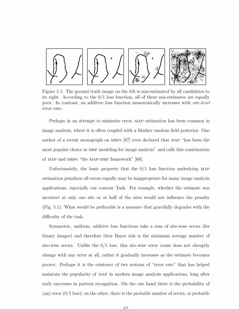
Figure 5.1: The ground truth image on the left is mis-estimated by all candidates toits right. According to the 0/1 loss function, all of these mis-estimates are equallypoor. In contrast, an additive loss function monotonically increases with site-levelerror rate.

Perhaps in an attempt to minimize error, map estimation has been common in

image analysis, where it is often coupled with a Markov random field posterior. One

author of a recent monograph on mrfs [67] even declared that map “has been the

most popular choice in mrf modeling for image analysis” and calls this combination

of map and mrfs “the map-mrf framework” [68].

Unfortunately, the basic property that the 0/1 loss function underlying map

estimation penalizes all errors equally may be inappropriate for many image analysis

applications, especially our contour Task. For example, whether the estimate was

incorrect at only one site or at half of the sites would not influence the penalty

(Fig. 5.1). What would be preferable is a measure that gracefully degrades with the

difficulty of the task.

Symmetric, uniform, additive loss functions take a sum of site-wise errors (for

binary images) and therefore their Bayes risk is the minimum average number of

site-wise errors. Unlike the 0/1 loss, this site-wise error count does not abruptly

change with any error at all, rather it gradually increases as the estimate becomes

poorer. Perhaps it is the existence of two notions of “error rate” that has helped

maintain the popularity of map in modern image analysis applications, long after

early successes in pattern recognition. On the one hand there is the probability of

(an) error (0/1 loss); on the other, there is the probable number of errors, or probable

67

error rate (additive loss). At low noise levels, the difference between additive and 0/1

losses may be small. At high noise levels, however, Marroquin observed empirically

that map estimates of binary fields are particularly poor compared to estimates based

on an additive loss [71].

5.1.3 Minimum Mean Squared Error Filtering

For binary image problems, this additive loss function is equivalent to the squared-

error loss, or the sum of the squares of the differences between the true unknown and

the estimate. Thus minimizing the additive loss amounts to choosing that binary

field that minimizes the mean squared error (mmse), or to computing

u>0 = arg minb∈0,1|I|

m||U>0 − b||2 (5.2)

= arg minb∈0,1|I|

∑

i

m(U>0

i − bi)2

= (arg minb1∈0,1

m(U>0

1 − b1)2, . . . , arg min

b|I|∈0,1

m(U>0

|I| − b|I|)2), (5.3)

where the last line follows from the second because the terms in the sum of positive

numbers can be optimized independently. Thus the additive loss provides an added

benefit in complexity: we have a separation of the joint estimation problem over

2|I| possibilities into |I| single-site problems of two possibilities each. Also, the |I|

separate expectations are taken with respect to the marginal distributions p(u>0i |m),

not the complicated joint distribution. In real-valued problems, one can expect the

marginals to be better behaved (smoother) than the joint, since each marginalization

is an integration process. (In this binary problem, the marginals are so “smooth”

they are a function of a single number!) Thus mmse estimation many not only be

more relevant to image analysis than map estimation, it may be easier as well.

68

5.1.4 Bounding the MMSE Estimate of the Binary CIRF

with a Thresholded Posterior Mean of the CIRF

Now that we have refined our original Task to that of computing the mmse estimate

u>0(m) of the binary cirf U>0 given measurements m, we would like to articulate

this goal in terms of the (non-binary) cirf U , for which we have a complete and

tractable statistical characterization.3 While it is obvious that U>0 and U are related,

the extent to which knowledge about U can help us in estimating U>0 is not. In this

section we show that u>0(m) and a thresholding of

mU are intimately related by a

simple inequality.

Because the squared-error loss is additive, we saw in (5.3) that we can focus on

the problem of finding the mmse estimate u>0(m) at site i, which can be expressed

as

u>0i(m) = arg min

bi∈0,1

m(U>0

i − bi)2

= arg minbi∈0,1

m(U>0

i )2 − 2bi

mU>0 + b2i

= arg minbi∈0,1

(

mU>0i − bi)

2

=

1, if

mU>0i ≥ 1

2

0, else

=:

mU>0i ≥ 1/2. (5.4)

Thus the mmse estimate of our binary field is its thresholded posterior mean [71],

suggesting that we first seek to relate the posterior means of U>0i and Ui, and then

threshold.

3The original intent was to exploit the statistics of U>0 directly. The cirf is used insteadbecause stronger results could be derived.

69

Before pursuing that relationship, we first study an intermediary, the hitting

random field H, where Hi ∈ 0, 1, 2, . . . is the total number times that site i was hit

by any curve Markov process. Observe that the binary cirf is a simple thresholding

of the hitting random field, i.e.,

U>0i =

Hi > 0, (5.5)

and so any function of U>0 is also a function of H. In particular, while it might

appear most natural to assume that our measurements are a corrupted version of

the binary cirf U>0, there is no loss in generality in assuming that our measurement

random field M is a function M(H,N), where N is some noise vector independent

of the curves.

Let τi denote the average amount of time that the curve Markov process spends

in site i each time it hits i (without conditioning on m). It can be shown that

τi = −1/qii, where Q = (qij) is the generator of the killed Markov process [22] (if

the Markov processes is spatially homogeneous (see §5.6.3), then τi does not vary

with i). The following lemma relates the posterior means of the curve indicator and

hitting random fields by the scalar factor τi.

Lemma 3. Suppose that m is a realization of the measurement random field M =

M(H,N), where noise N is independent of the curve Markov processes (and thus the

hitting random field H and the cirf U). Then:

mUi = τi

mHi, ∀i ∈ I,

where τi is the average time spent in site i per visit.

70

proof. Let t(n)i , n = 1, . . . , Hi denote the (random) holding time spent in site i dur-

ing the n-th hit by a curve Markov process. (The ordering of the hits is immaterial;

the index n merely distinguishes the different time intervals.) Recall from the the-

ory of continuous-time, discrete-state Markov processes [86] that the holding times

are independent, exponentially-distributed random variables of mean τi, when con-

ditioned upon the sequence of states taken by the processes. It follows that the t(n)i

(n = 1, . . . , Hi) are independent exponentially-distributed random variables of mean

τi, given H. We can write the cirf at site i as Ui =∑Hi

n=1 t(n)i , and therefore

MUi =

[Ui|M ] =

[∑Hi

n=1 t(n)i |M ] =

[

[∑Hi

n=1 t(n)i |H,M ]|M ]=

[∑Hi

n=1

[t

(n)i |H,M ]|M ]. We

now observe that[t

(n)i |H,M ] =

[t

(n)i |H] = τi, where t

(n)i given H is independent of

M because (1) M is only a function of H and N , and (2) N is independent of t(n)i

(because it is determined by the curve Markov processes, which are independent of

N). The result follows because∑Hi

n=1 τi = τiHi.

Given this connection between U andH, we are now in a position to show that the

thresholded posterior mean of the cirf U is an upper bound on the mmse estimate

u>0 of the binary curve random field U>0.

Proposition 6. Suppose that m is a realization of the measurement random field

M = M(H,N), where noise N is independent of the curve Markov processes. Then

the mmse estimate of U>0 given m is bounded from above by a thresholded posterior

mean of the cirf, or

u>0i(m) =

mU

>0i ≥ 1/2

≤

mUi ≥ τi/2 , ∀i ∈ I, (5.6)

where τi is the average time spent in site i per visit.

71

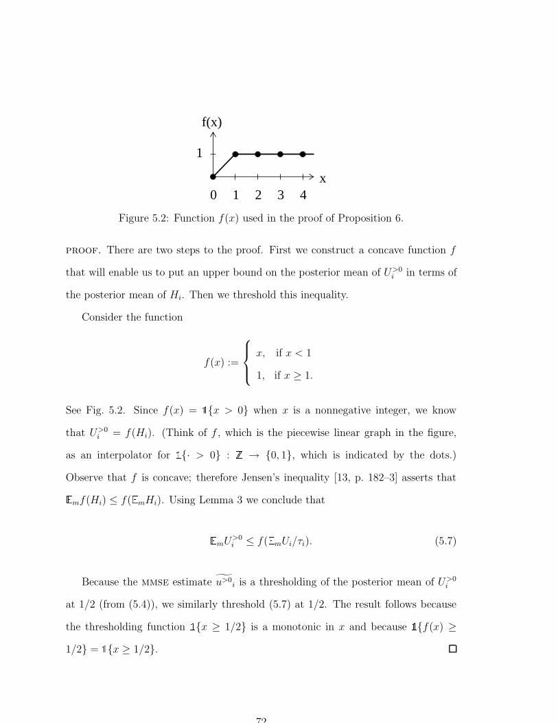
x

f(x)

1

10 2 3 4

Figure 5.2: Function f(x) used in the proof of Proposition 6.

proof. There are two steps to the proof. First we construct a concave function f

that will enable us to put an upper bound on the posterior mean of U>0i in terms of

the posterior mean of Hi. Then we threshold this inequality.

Consider the function

f(x) :=

x, if x < 1

1, if x ≥ 1.

See Fig. 5.2. Since f(x) = x > 0 when x is a nonnegative integer, we know

that U>0i = f(Hi). (Think of f , which is the piecewise linear graph in the figure,

as an interpolator for · > 0 :

→ 0, 1, which is indicated by the dots.)

Observe that f is concave; therefore Jensen’s inequality [13, p. 182–3] asserts that

mf(Hi) ≤ f(

mHi). Using Lemma 3 we conclude that

mU

>0i ≤ f(

mUi/τi). (5.7)

Because the mmse estimate u>0i is a thresholding of the posterior mean of U>0

i

at 1/2 (from (5.4)), we similarly threshold (5.7) at 1/2. The result follows because

the thresholding function x ≥ 1/2 is a monotonic in x and because

f(x) ≥

1/2 = x ≥ 1/2.

72

Proposition 6 enables us to connect the (non-binary) cirf U to our binary de-

cision problem. This upper bound has a simple interpretation: the thresholded

posterior mean of the cirf can have no more misses than u>0; it can only have more

false positives. Because of this close relationship, in the rest of this thesis we shall

approximate the mmse estimate of U>0 given m with the thresholded posterior mean

of the cirf U . Since thresholding is trivial, we shall define our filtering problem to

be the computation of the cirf posterior mean

mU only. In statistical language,

the posterior mean

mU is known as the regression of U on m.

It is well-known that the posterior mean is the mmse estimate for real-valued ran-

dom variables (see [14, p. 68], [13], or [41, p. 483]), and therefore our goal is equivalent

to the computation of the mmse estimate of U given m. In many non-Gaussian cases

the posterior mean can be difficult to compute; in our context, however, we are fortu-

nate to have tractable formulas for the cumulants and moment generating functional

to simplify our computations. Before developing linear and nonlinear mmse cirf

filters that leverage these formulas, we shall present our observation model.

5.2 Observation Models and Likelihoods

Although the cirf has been the focus of Chapters 2 and 3, it is only part of the

contour inferencing story: the prior. Another key component is the likelihood, which

we consider here.

5.2.1 The Gaussian Likelihood

The likelihood represents how our ideal contour image relates to the measurements,

and therefore it characterizes the corruptions in local edge and line operator re-

sponses, or how observed contours are non-ideal. For example, edges are blurry, in

73

the sense that edge operators have an associated scale [129, 59, 26]. Equally impor-

tant is the random noise in edge measurements: even for intensity images with high

signal-to-noise ratio (snr), edges can still be noisy for two reasons. Most funda-

mentally, edge detection requires differentiation, which amplifies noise. In addition,

when the local contrast (i.e., signal) is low, the local snr drops for fixed sensor noise.

One way of specifying such sources of corruption is to write an observation equa-

tion that relates the unknowns to the observations. Although one can consider much

more general models, both for concreteness and simplicity we assume that the mea-

surements are a linear function of the cirf plus Gaussian noise N with zero-mean

and covariance operator ΣN , or M = BU+N , where B ∈ |I|×|I| is a linear operator

used to model the local edge or line filtering and blur. This observation equation

gives rise to the following Gaussian likelihood that models noise and blur:

p(m|u) = (2π)−|I|/2(det ΣN)−1/2 exp

[−1

2〈m− Bu,Σ−1

N (m−Bu)〉].

We stress that the linear operator B is quite flexible: not only can it be a standard

blur operator, but it can also represent more fundamental aspects of observation.

For example, in the case where I is the discretized three-dimensional (x, y, θ)-space

and M is a two-dimensional image, B would be the (discrete) linear projection that

integrates along θ. It can also capture the image derivatives used in local edge and

line operators as well, and thus the operator B need not even perform blurring. Noise

structure can be partially captured by non-diagonal noise covarainace operator ΣN ,

i.e., the correlated noise can be handled.

One may object with this likelihood model on the grounds that the measurement

is a now function of the cirf U , not the more natural binary cirf U>0 or even hitting

random field H. Indeed, Proposition 6 required that M = M(H,N), not M =

74

M(U,N), and we are therefore introducing another approximation with this cirf-

dependent likelihood model. The key difference between U and H is an additional

holding-time “noise” from the continuous-time, discrete-state Markov processes (see

the proof of Lemma 3). At least for those cases where the kernel for B is positive

and has large support (i.e., B is a large scale blur operator) and where τi = τ for

all i, the approximation BU ≈ τBH may be very good because the holding times

are independent, have finite variance and therefore the central limit theorem applies.

As the spatial discretization becomes finer but the absolute scale of the blur kernel

remains fixed, this large (discrete) scale requirement will be met.

5.2.2 Log-Likelihoods with Quadratic Dependence on the

CIRF

The Gaussian is an example of a more general class of quadratic log-likelihoods with

ln p(m|u) = ε〈a + Au, u〉+ constant, (5.8)

where A is a symmetric, nonnegative definite matrix, and vector a and the constant

are functions of the measurement vector m. To relate this class to the Gaussian

likelihood (5.2.1), we set εa = B∗Σ−1N m and εA = −1

2B∗Σ−1

N B. The coefficient ε is

introduced to capture the degree of noise; when the noise is white (ΣN = σ2NI),

this coefficient could be used to represent the inverse noise variance, or ε = σ−2N .

Although for the Gaussian, the vector a is linear in the measurements, the quadratic

log-likelihood allows a to be a general functions of m. Indeed, all of the nonlinear

filters we shall be presenting allow a to be any (measurable) function of m. Some

non-Gaussian observation models can be handled using this freedom in a and A by

a change of variables to a Gaussian model. For example, multiplicative noise can be

75

modeled using a logarithmic change of variables to additive Gaussian white noise.

Molina et al in effect used this technique for restoring astronomical images [79,

Equation (24)]. We present another non-Gaussian example of the quadratic log-

likelihood next.

5.2.3 Exploiting Empirical Distributions of Local Operators

Suppose we have training data in the form of a number of curve images and their

corrupted counterparts. How could we use information gathered from this data to

empirically derive our likelihood function?

One way of doing this is to construct an observation model that only considers

whether a contour hit a site or not by determining the “on” and “off” edge re-

sponses [35]. To formalize this, we set up a likelihood in terms of the binary cirf

U>0, where U>0i = 1 only when at least one of the contours passed sometime through

site i, and 0 otherwise. To simplify the situation, we focus on the class of condition-

ally independent, local likelihoods: p(m|u>0) = p(m1|u>01 ) · · · p(m|I||u>0

|I|). Follow-

ing [35, 133], we consider two distributions over measurements at site i: the “on” dis-

tribution pon(mi) := p(mi|u>0i = 1) and “off” distribution poff(mi) := p(mi|u>0

i = 0).

(Spatial homogeneity is implicit here: the “on” and “off” distributions are assumed

not to depend on i, although this can be relaxed.) Such distributions can ap-

proximated with histograms obtained from the training data [63]. It follows that

ln p(m|u>0) =∑

i u>0i ln pon(mi)

poff(mi)+∑

i ln poff(mi). Letting τ again be the average

amount of time that the Markov process spends in a site per hit of the site, ob-

serve that Ui/τ and U>0i are equal on average, as long as each site gets hit at most

once. Ignoring this latter condition for a moment, one can heuristically try to cre-

ate a likelihood conditioned on u by replacing u>0 with u/τ above: ln p(m|u) ≈

ε∑

i aiui + constant(m) = ε〈a, u〉+ constant(m), where ai = ai(mi) := τ−1 ln pon(mi)poff(mi)

76

and ε = 1. To ensure normalizability, we include a term ε〈Au, u〉 in the likeli-

hood, where A = − 12I, and so obtain a valid quadratic log-likelihood in the form of

(5.8). Observe that this log-likelihood has quadratic dependence on u, but possibly

nonlinear dependence on m. The norm-squared ||u||2 = −2〈Au, u〉 measures the

self-interaction of the cirf; specifically, this term is∑

i u2i , or the sum of the mea-

sure of the self-intersections and crossings of the curves as described in §3.1.1. This

quadratic term therfore penalizes violations of the above condition that a site gets hit

at most once. (To further penalize intersections, one can replace the old prior P (du)

with a modified prior Z−1β exp(−β||u||2)P (du), where Zβ :=

∫exp(−β||u||2)P (du).

See §5.3 for notation.) This empirical model can also be combined with the 3-d to

2-d projection discussed in the Gaussian case by modifying A appropriately if the

training observations are two-dimensional.

5.3 The Posterior Distribution

In this section we set up some notation for gluing together the likelihood with the

prior to form the posterior. We write the cirf prior as P (du) := PU(du) = U ∈

du and combine it with the likelihood p(m|u) := pM |U(m|u) using Bayes’ rule to

obtain the posterior P (du|m) = p(m|u)P (du)p(m)

, where p(m) :=∫p(m|u)P (du). If U had

a density pU(u), then P (du) = pU(u)du. Instead we use the general notation P (du)

for the distribution of U since a density exists for cirf U only in a generalized sense.

Specifically, at each site i there is positive mass for ui = 0. Combined with our

quadratic log-likelihood (5.8), the posterior is therefore

P(ε)(du) = Z−1(ε) exp(ε〈a+ Au, u〉)P (du),

77

where Z(ε) :=∫

exp(ε〈a + Au, u〉)P (du) and the subscript with ε indicates the

quadratic log-likelihood. Note that although we do not have an explicit expres-

sion for the prior P (du) (and therefore no explicit expression for this posterior), we

can indirectly use the prior for U through its moment generating functional (mgf).

An even simpler way of using the mgf is via the cumulants. We start by applying the

mean and covariance in §5.4 on linear filtering, and later use higher-order statistics

for Volterra filters in §5.5. Finally, we exploit all orders of the cirf statistics by

explicitly using the mgf to represent a filter in §5.7.

5.4 The Linear Case

Although one may consider all statistical properties of the curve indicator random

field, even the pair-wise relations express information critical to enhancing curves.

As Gaussian random fields are fully defined by their means and covariances, in this

section we simplify our contour filtering problem by replacing the cirf prior with

a Gaussian approximation pGaussian(u) with the mean µU and covariance ΣU from

Corollary 4. Under this approximation, we can write the log-prior as

ln pGaussian(u) = −1

2〈u− µU ,Σ

−1U (u− µU)〉+ constant(m)

= 〈Σ−1U µU , u〉 −

1

2〈Σ−1

U u, u〉+ constant(m).

Combined with the quadratic log-likelihood (5.8) we get the following quadratic log-

posterior (implying the posterior is Gaussian):

ln pGaussian(u|m) = ln p(m|u) + ln pGaussian(u) + constant(m)

= 〈εa + Σ−1U µU , u〉+ 〈

(εA− 1

2Σ−1

U

)u, u〉+ constant(m).

78

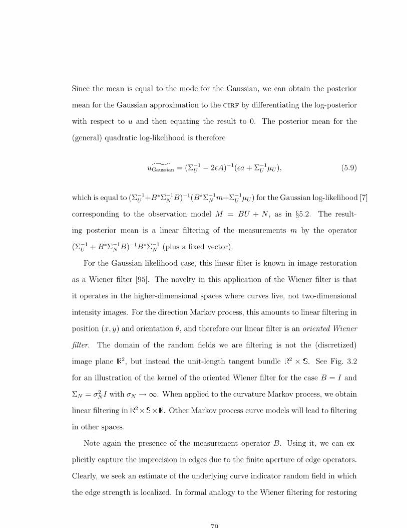
Since the mean is equal to the mode for the Gaussian, we can obtain the posterior

mean for the Gaussian approximation to the cirf by differentiating the log-posterior

with respect to u and then equating the result to 0. The posterior mean for the

(general) quadratic log-likelihood is therefore

uGaussian = (Σ−1U − 2εA)−1(εa + Σ−1

U µU), (5.9)

which is equal to (Σ−1U +B∗Σ−1

N B)−1(B∗Σ−1N m+Σ−1

U µU) for the Gaussian log-likelihood [7]

corresponding to the observation model M = BU + N , as in §5.2. The result-

ing posterior mean is a linear filtering of the measurements m by the operator

(Σ−1U +B∗Σ−1

N B)−1B∗Σ−1N (plus a fixed vector).

For the Gaussian likelihood case, this linear filter is known in image restoration

as a Wiener filter [95]. The novelty in this application of the Wiener filter is that

it operates in the higher-dimensional spaces where curves live, not two-dimensional

intensity images. For the direction Markov process, this amounts to linear filtering in

position (x, y) and orientation θ, and therefore our linear filter is an oriented Wiener

filter. The domain of the random fields we are filtering is not the (discretized)

image plane 2, but instead the unit-length tangent bundle

2 × . See Fig. 3.2

for an illustration of the kernel of the oriented Wiener filter for the case B = I and

ΣN = σ2NI with σN →∞. When applied to the curvature Markov process, we obtain

linear filtering in 2× ×

. Other Markov process curve models will lead to filtering

in other spaces.

Note again the presence of the measurement operator B. Using it, we can ex-

plicitly capture the imprecision in edges due to the finite aperture of edge operators.

Clearly, we seek an estimate of the underlying curve indicator random field in which

the edge strength is localized. In formal analogy to the Wiener filtering for restoring

79

out-of-focus grey-scale images, the filter here is a means of de-blurring edge measure-

ment fields on 2 × . Such a sharpening effect has been viewed as non-maximum

suppression [39] or detection [51]. Other techniques for curve enhancement generally

do no explicitly model blur at all. In contrast, blur is straightforward to include in

this random field model.

Okajima [88] has independently proposed a closely-related Wiener filter for model-

ing the horizontal connections between complex cells in V1. Okajima’s filter operates

in position and spatial frequency, and he exploits translation invariance to simplify

his model, although he does not consider the additional rotation invariance suggested

by 2 × and possessed by the oriented Wiener filter (see also §4.1). Interestingly,

the coefficients of his model were learned from the responses of Gabor filters to a

number of straight-line images and bear a qualitative resemblance to ours, which, in

contrast, were derived from the blur operator B, the noise model, and curve indicator

random field covariance.

5.4.1 Why Simple Cells and Local Edge Operators

are Elongated

When Hubel and Wiesel reported the existence of cells in primate visual cortex that

respond to edge and bar stimuli, they established a connection between physiology

and geometry [45]. Unfortunately, no theory deriving the qualitative features of the

receptive field for even their “simple cell” was provided. Recall that there are two

key “directions” of the receptive field: normal and tangential to the major axis of

the receptive field. Since the receptive fields of simple cells resemble the kernels of

(oriented) local edge and line operators, understanding the rationale for one explains

the other. The normal profile is generally understood functionally as a kind of blurred

80

differentiation [11, 93] using the theory of regularization. The tangential profile, with

its elongated structure, is more poorly understood. Nonetheless many have designed

elongated filters where the tangential profile is explained using a variety of theories,

such as an uncertainty principle [16], Hilbert space representations [46], or increased

noise immunity [11]. The cirf linear filter corresponding to the direction process

provides a much simpler explanation for the simple cell receptive field: it is tuned

to find contour structure in the visual world. Using this idea, one can relate the

length and aspect ratio of the simple cell receptive field to the expected length and

curvature bound on contours that the cell can measure.

But does the curve indicator random field provide more than a contour-based

explanation for elongated linear filtering? To answer this question, we shall have to

go beyond the connection between linear filtering and second-order statistics.

5.5 Volterra Filters and Higher-Order Statistics

Volterra filters constitute one class of nonlinear filters that subsumes linear fil-

ters [107]. Even though most work on Volterra filtering is done on time-domain

sequences, we shall apply these ideas to multidimensional signals (functions on 2× ,

for example) or on vectors m = (mi), where i is a site in I. By definition, the output

of a Volterra filter is a polynomial4 function of the input signal. Although Volterra

filters are (generally) nonlinear, they can always be represented as a linear function of

products of the input m. A k-th order Volterra filter is a linear function of 0- through

k-fold products of the input; for example, a quadratic (second-order) Volterra filter

can be written as a linear combination of a constant, the input mi at site i, and the

4One must distinguish the nonlinear polynomial (Volterra) filters that we consider here fromthose linear filters whose kernel is based on some polynomial, e.g., a Hermite polynomial.

81

products mimj of input at sites i and j. A linear filter (plus a constant) is simply a

first-order Volterra filter.

Analogous to the connection between mmse linear filters and second-order statis-

tics, mmse Volterra filters are related to higher-order statistics. The key lies in

exploiting the fact that Volterra filters are linear functions of products of the input.

Instead of the actual inputs mi, the idea is to focus on an “apparent” set of in-

puts 1 ∪ mi ∪ mi ·mj ∪ · · · mi1 ·mi2 · · ·mik, and so reduce the derivation of

the (polynomial) Volterra filter on the actual inputs to the design of a linear filter

on the apparent inputs. Because mmse linear filters can be derived by solving a

linear system (see §5.4) in terms of the second-order statistics of the input and the

unknown U , one can therefore compute a mmse Volterra filter by solving a linear

system in terms of the second-order statistics of the apparent input and unknown,

or the (2k)-th order statistics of the input and unknown. In the context of discrete-

time systems, such a linear system for Volterra filtering in terms of higher-order

statistics was presented in [1] and later in [92, 10]. Based on empirical estimates of

higher-order statistics, one-dimensional low-order (quadratic and occasionally cubic)

Volterra filters have been designed [84, 134].

The generality of Volterra filtering can be immobilizing, for one must specify

a large number of coefficients in designing one. In filtering a vector of length n

(mathematically, a mapping from n to

n), a linear filter requires O(n2) coeffi-

cients, whereas a general k-order Volterra filter requires O(nk+1) coefficients. For

applications in vision, the appropriate length n can be truly large: for images n is

on the order of a million, and for the discretized 2 × , n can be even a hundred

times that. Not only is directly solving the linear system for the mmse Volterra

filter unthinkable in these dimensions, just estimating such higher-order statistics

82

requires enormous amounts of data. Applying the Volterra filter in the general case

is similarly burdensome.

Symmetries and structural simplifications of any kind are essentially the only hope

for taming the generality of the Volterra filter. One obvious symmetry is homogene-

ity: the kernel of the filter is the same irrespective of which portion of the image it is

applied. This brings the number of coefficients need down to O(nk) from O(nk+1) for

the k-th order Volterra filter. Such homogeneity of the filter is a consequence of the

statistical homogeneity of the unknown signal and noise, and amounts to stationarity

for one-dimensional signals. Other simplifications arise when the unknown signal U

is in some parametric family (e.g., ARMA models in one-dimension [84]) or when the

Volterra filter is assumed to have a particular structure, such as factorizability [62]

or a tensor product basis representation [87]. In vision, quadratic filters have been

applied for local contour detection independent of phase (e.g., the contour’s edge

vs. line characteristics) [81], and general polynomial filters have been linked to the

characterization and discrimination of textures [65]. Maass has made an interesting

connection between Volterra filters and neural network dynamics [69]. In the case of

contour filtering, we shall now see that the special structure of the cirf cumulants

(§3.4.3), combined with a Taylor series expansion in inverse noise level, makes mmse

Volterra filtering of noisy images possible.

5.6 Deriving CIRF Volterra Filters

via Perturbation Expansion

Here we derive linear, quadratic and even cubic Volterra filters for the cirf U ob-

served in white Gaussian noise. In principle, similar techniques can also be used

for filtering the cirf observed with a log-likelihood polynomially dependent on U .

83

The basic idea will be to observe the dependence of the log-likelihood on a small

parameter (the inverse noise variance), and to perform a perturbation expansion in

that parameter. We shall study this perturbation expansion first, developing the

notation and tools that will be necessary to carry it out.

Suppose we have a random vector X = (X i) (superscripts here index the compo-

nent of the vector and do not represent taking a power) with prior distribution P (dx)

(with known cumulants) and posterior distribution P(ε)(dx) = Z−1(ε) exp(εf(x))P (dx),

where ε is a small real number, f(x) = 〈a + Ax, x〉 is a real-valued function of x,

a = (ai) is a constant vector, A = (aij) is a symmetric, negative definite linear oper-

ator, and the normalizing constant Z(ε) is equal to∫

exp(εf(x))P (dx). Observe that

this situation applies exactly to the cirf in Gaussian white noise, where U = X,

ε = σ−2N , a = m, aij = −1

2δij and f(x) = f(u) = 〈m − 1

2u, u〉. Note that we do

know all the cumulants of the cirf prior U from Chapter 3. Given that that the

main application for this thesis is the filtering of extremely noisy contour images,

understanding how to optimally filter as σN →∞, or equivalently, as ε→ 0, is very

important. To avoid being distracted by the particulars of the application of this

idea to the cirf, let us now focus on the problem of estimating X. We can apply

the results we derive to the cirf later.

Recalling that the mmse estimate of X is the posterior mean

(ε)X, our task

is to compute a Taylor series expansion of the posterior mean around ε = 0. To

foreshadow the results to come, we shall see that up to order ε3 the expansion of the

posterior mean to order εk is a k-th order Volterra filter requiring cumulants of up

to the (k + 1)-th order for the cirf.5

5This assumes that the cirf is based on an approximately self-avoiding Markov process; other-wise, (2k + 1)-th order cumulants would be required.

84

Now, observe that the (posterior) mean can be computed by differentiating the

logarithm of the normalizing constant,or

∂ lnZ(ε)

∂(εai)= Z−1

(ε)

∫∂ exp(ε〈a+ Ax, x〉)

∂(εai)P (dx) =

∫xiP(ε)(dx) =

(ε)X

i. (5.10)

Therefore to get a Taylor series for the posterior mean, we need only get a Taylor

series for lnZ(ε) and then differentiate with respect to εai.

Where do we get a Taylor series for lnZ(ε)? Observe that the normalizing constant

Z(ε) is just the moment generating functional of the random vector Y = f(X) in

disguise, or, equivalently, Y has the cumulant generating functional cgfY (ε) such

that

lnZ(ε) = ln

∫exp(εf(x))P (dx) = ln

∫exp(εy)P (dx) = lnmgfY (ε) = cgfY (ε).

(5.11)

But the coefficients in a Taylor series expansion of a cumulant generating functional

are by definition the cumulants, and therefore we need to obtain the cumulants of

Y = f(X), a (quadratic) polynomial inX. Unfortunately, the cumulants of Y are not

directly known; we must somehow calculate them in terms of the (known) cumulants

of X.

5.6.1 Tensors and Generalized Cumulants

Without appropriate tools, calculating the cumulants of a polynomial can be extraor-

dinarily difficult. To aid in this task, McCullagh has developed a tensor formalism

for representing moments, cumulants, and so-called generalized cumulants [75, 76].

Elsewhere in early vision, tensors have previously been used to represent blurred im-

age derivatives via the multiscale local jet [33, 31, 32] and to summarize local tangent

85

information for relaxation labeling [21] and linear filtering (“tensor voting”) [39]. We

now review McCullagh’s formalism.

For the purposes of this discussion, a tensor is an indexed array of numbers, for

example aij or bijk , where indices such as i, j, k can appear as superscripts or subscripts

and vary over a set of index values, e.g., i ∈ I. Tensors are multiplied together by

multiplying the corresponding array entries (as numbers), as in aiXi or bijdi, although

we shall generally adopt the summation convention. In this convention, an index that

appears in both a subscript and a superscript is assumed to be summed over; e.g.,

aiXi :=

∑i aiX

i, and aijYj :=

∑j aijY

j. An index that appears twice or more as

a superscript, but not as a subscript (or vice versa) is not assumed to be summed

over; so, for example, we do not assume that gijgjk is equal to∑

j gijgjk, but we

do assume that ajgijgjk :=

∑j ajg

ijgjk. The summation convention often makes for

pithy expressions, but we shall not hesitate from writing out the sum explicitly if it

helps to reduce ambiguity.

Moments and cumulants can conveniently be represented using tensors, as follows.

The first momentX i will be denoted by κi

X and the second momentX iXj by κij

X .

More generally, the k-th momentX i1 · · ·X ik of the i1-th through ik-th components

of X will be indicated by κi1···ikX = κi1···ik , where the subscript X will be dropped

if understood. Cumulants will be written in a similar fashion, except that commas

will separate the indices; we define κi,j,k := cumX i, Xj, Xk, for example (where

X is understood). In general, the k-th cumulant of X i1 through X ik is denoted by

κi1,...,ik := cumX i1, . . . , X ik. Observe that κi denotes both the first moment and

first cumulant of X i, which is appropriate since they are equal.

A generalized cumulant of random vector X is simply a cumulant of products

of the components of X, such as cumX i, XjXk. McCullagh has suggested the

86

convenient notation

κij,k,lmn := cumX iXj, Xk, X lXmXn (5.12)

for generalized cumulants, where the commas in the superscript separate blocks

of indices, with each block corresponding to a product of components of X and

where these products are separated by commas in the (ordinary) cumulant (as on

the right hand side of (5.12)). Due to the symmetry of both (ordinary) cumulants

and products of components in their indices, the generalized cumulant is symmetric

in its arguments in two senses: (1) the order of the blocks is irrelevant and (2) the

order of the indices within each block is irrelevant. Indices cannot be moved from

one block to another, however, and therefore κi,jk is equal to κkj,i but not equal to

κij,k, for example. Observe that an ordinary cumulant of k-th order is a generalized

cumulant with k blocks of indices, with just one index per block, or κi1,...,ik . In

contrast, a k-th order moment is a simply a generalized cumulant with one block of

k indices, or κi1···ik . Thus the generalized cumulant indeed is a generalization of the

statistical constructions of moments and cumulants.

How can a generalized cumulant be expressed in terms of ordinary cumulants?

McCullagh has derived a formula for generalized cumulants as a sum of products

of ordinary cumulants. Because we use this formula later, we shall set it up here.

Observe that a generalized cumulant with α blocks involving a total of β random

variables can be written as κ(

), where

:= v1, . . . , vα is a partition of β indices

into α non-empty blocks v1, . . . , vα of indices. Now, any such partition can be written

as a graph with β vertices, where one vertex is for each random variable or random

vector component. All vertices corresponding to each block vj of the partition will

be connected by edges, but no two vertices in distinct blocks will be linked by an

87

edge. In this way, a partition

corresponds to a graph that is a union of α complete

graphs, but with no two such complete subgraphs being connected. Thus

will also

denote this corresponding graph. Given any other partition ′ of the same set of

indices (and its corresponding graph), the edge sum ⊕ ′ is a graph in the same

vertices where the set of edges is the union of the edges for

and ′. Now we

can state McCullagh’s formula for the generalized cumulant in terms of products of

ordinary cumulants:

κ(

) =∑

′

κ(v′1) · · ·κ(v′n), (5.13)

where the sum extends over all n-block partitions ′ := v′1, . . . , v′n such that

⊕ ′

is a connected graph. The factors κ(v′j) in the sum are ordinary cumulants in the

indices in block v′j of the partition ′.

To illustrate McCullagh’s result, consider the generalized cumulant corresponding

to the partition

= 1, 2, 3, 4, 5, 6 with α = 4 blocks and β = 6 indices.

While each block of partition ′ = 1, 3, 2, 4, 5, 6 joins a block of

, the

edge sum ⊕ ′ is not connected (because 5, 6 is disconnected from the other

nodes) and so there is no term in the sum in (5.13) corresponding to ′. However, the

partition ′′ = 1, 2, 3, 4, 5, 6 does contribute the term κ(1, 2, 3)κ(4, 5, 6) =

κ1,2,3κ4,5,6 to the sum because ⊕ ′′ is connected. Using the formula, one obtains,

for example,

κi,jk = κi,j,k + κi,jκk + κi,kκj = κi,j,k + κi,jκk[2],

where the bracketed number on the right of a term is the number of partitions

of similar form that should be included in the sum. In this case, κi,jκk[2] equals

κi,jκk + κi,kκk. Although this bracket notation can be ambiguous (e.g., note that

term κj,kκi, although of similar form, is not implied by the above use of κi,jκk[2]), it

is useful in avoiding truly long enumerated lists. Another example of McCullagh’s

88

formula is

κi,j,kl = κi,j,k,l + κkκi,j,l[2] + κi,kκj,l[2].

Applied to the third moment κijk, the formula requires a sum over all partitions

of i, j, k (because

= i, j, k is already connected); and applied to ordinary

cumulant κi,j,k,l (with

= 1, 2, 3, 4), the formula is satisfied by exactly

one partition ′ = 1, 2, 3, 4 connecting all nodes. Thus McCullagh’s formula

succinctly expresses generalized cumulants in terms of a sum of products of ordinary

cumulants.

5.6.2 Cumulants of Polynomials

With the generalized cumulant formula, we now need only express the cumulants

of our polynomial Y = f(X) in terms of the generalized cumulants of X. By the

linearity of expectation and of cumulants [112], cumulants of homogeneous polyno-

mials such as aiXi and aijX

iXj can be computed straightforwardly. For example,

[aiX

i] = cumaiXi = ai cumX i = aiκ

i and

var(aijXiXj) = cumaijX

iXj, aklXkX l = aijakl cumX iXj, XkX l = aijaklκ

ij,kl

= aijakl(κi,j,k,l + κi,kκj,l[2] + κiκj,k,l[2] + κkκi,j,l[2] + κiκkκj,l[4]),

using the generalized cumulant formula. Although one can compute the cumulants

of general polynomial transformations of a random variable [76, 62 ff.], here we focus

on our case of interest, Y = 〈a+AX,X〉 = aiXi + aijX

iXj =: (A1 +A2)X =: PX,

where we use the notation P = A1 + A2 for our polynomial operator with linear

part A1 and quadratic part A2. One can [76, p. 63] express the cumulant generating

89

functional in terms of the cumulant tensors κ of X using the formal expansion

cgfY (ε) = exp(εP)κ = (1 + εP + ε2PP/2! + ε3PPP/3! + · · · )κ.

The terms in this expansion are determined by expanding the polynomial operator

into a sum of homogeneous polynomials, as follows:

Pκ = (A1 + A2)κ = aiκi + aijκ

ij

and

PPκ = (A1 + A2)(A1 + A2)κ

= A1A1κ+ A1A2κ+ A2A1κ + A2A2κ

= aiajκi,j + aiajkκ

i,jk + aijakκij,k + aijajkκ

ij,jk

= aiajκi,j + aiajkκ

i,jk[2] + aijajkκij,jk.

Observe there is only one block of indices in the generalized cumulants in Pκ, but

there are two blocks for the generalized cumulants in PPκ. Higher order terms

behave similarly, as we now observe in our sought-for expression of the cumulant

generating function of the polynomial Y in terms of the generalized cumulants of X:

cgfY (ε) = ε(aiκ

i + aijκij)

+ε2

2

(aiajκ

i,j + aiajkκi,jk[2] + aijaklκ

ij,kl)

+ε3

6

(aiajakκ

i,j,k + aiajaklκi,j,kl[3] + aiajkalmκ

i,jk,lm[3] + aijaklamnκij,kl,mn

)

+ε4

24

(aiajakalκ

i,j,k,l + aiajakalmκi,j,k,lm[4] + aiajaklamnκ

i,j,kl,mn[6]

+aiajkalmanoκi,jk,lm,no[4] + aijaklamnaopκ

ij,kl,mn,op)

+O(ε5).

90

This expression can be further simplified by observing that all of the bracketed

numbers representing permutations become scalar factors by relabeling indices ap-

propriately. To obtain the posterior mean

(ε)X, by (5.10) and (5.11) we need only

differentiate cgfY (ε) with respect to εar, as follows:

(ε)X

r = κr

+ε(aiκ

r,i + aijκr,ij)

+ε2

2

(aiajκ

r,i,j + 2aiajkκr,i,jk + aijaklκ

r,ij,kl)

+ε3

6

(aiajakκ

r,i,j,k + 3aiajaklκr,i,j,kl + 3aiajkalmκ

r,i,jk,lm

+aijaklamnκr,ij,kl,mn

)

+O(ε4). (5.14)

Expression (5.14) can be used directly to compute the posterior mean of a signal (with

known cumulants) that is corrupted by linear blur and (the limit of) large, possibly

correlated, Gaussian noise (for more general observation models, see §5.2.2). One

can derive linear (O(ε) terms), quadratic (O(ε2) terms), cubic (O(ε3) terms) and

other higher-order Volterra filters by systematically computing all of the generalized

cumulants of X in terms of its ordinary cumulants.

5.6.3 The CIRF: A Tractable Special Case

In the general case, the expansion of formula (5.14) is a lengthy and tedious task: each

generalized cumulant will become a possibly large number of products of ordinary cu-

mulants. In addition, the resulting computation naively suggested by the summation

convention would have high-order polynomial complexity, where the order depends

on the number of terms in the perturbation expansion, e.g., O(n7) operations for the

91

cubic filter, which has all the terms explicitly listed in (5.14). For n = 106, applying

the cubic filter would naively require on the order of (106)7 = 1042 operations. It

is little wonder, therefore, that this formula has not appeared in high-noise signal

processing or vision applications before.

Fortunately, the contour images modeled by the cirf have a special cumulant

structure that we can exploit (see §3.4.3). In addition, we invoke several realistic

assumptions that will both (1) significantly simplify the task of even writing down

the surfeit of terms and (2) reduce the computational complexity of the filters to

that of applying the Green’s operator G. For the direction process-based cirf, the

filter complexity becomes O(n logn), where n = |I|. We now consider these extra

assumptions in turn.

Spatial Homogeneity

For general purpose contour enhancement, we assume that any knowledge about

contour endpoint locations will be conveyed by the contour image itself. Equivalently,

one is indifferent to the starting and ending locations of each contour. As introduced

in §3.4.2, this amounts to setting the initial distribution µ and final weighting ν

proportional to a constant, e.g., µi = |I|−1, νi = λ−1, for all sites i ∈ I. Using the

notion of contour density η := Nλ/|I| (the average amount of contour per site) and

observing that G1 = λ1, a simple calculation shows that the k-th cumulant of the

spatially homogeneous cirf U at sites i1, . . . , ik becomes:

κi1,...,ik = cumUi1 , . . . , Uik = η∑

a∈permk

gia1 ia2 · · · giak−1iak . (5.15)

(Superscripts are used here in keeping with the tensor notation and summation con-

vention.) In addition, the Markov process Rt itself will be assumed to be spatially

92

homogeneous in the sense that shifts6 in the initial conditions give rise to corre-

sponding shifts in the solution to the corresponding Fokker-Planck diffusion. As a

consequence, the Green’s operator G = (gij) is constant along the diagonal, i.e.,

gii =: d, for all i ∈ I.

Low Contour Density

Another fact that we shall exploit is that, in a large number of images, contours

constitute a small fraction of the total image. For the cirf, this amounts to asserting

that the contour density η is small (0 ≤ η 1). In the continuum, an extreme form

of this claim certainly holds: the bounding contours in an image of smooth surfaces

in an occlusion relationship constitute a set of measure zero (with respect to the

standard area measure in the plane). In natural images it is easy to observe a variety

of sources of contours for which the low-density cirf is appropriate, such as occlusion

edges, highlights, surface markings (albedo discontinuities), and shadow boundaries.

A number of textures, in particular those where contour structure dominates regions,

may not appear to be modeled realistically by low-density cirfs, and indeed this

is the case if the underlying Markov process is planar Brownian motion. But when

using higher-dimensional Markov process contour models, even images with a large

number of crossing contours can be reasonably modeled with low-density cirfs. For

example, contours that cross in a two-dimensional image will not cross in 2 ×

unless they have the same orientation at the crossing point. Working with curvature

in 2 × ×

, even highly dense planar texture patterns are represented with lower

density as well.

6Depending on the Markov process, the shifts might include translations and rotations (e.g.,planar Brownian motion and Mumford’s direction process). In general the shifts will be the set oftransformations under which the Fokker-Planck equation is invariant (see [140] for some discussionof this).

93

The key consequence of low contour density is that the generalized cumulants

in (5.14) can be approximated with one corresponding joint cumulant, as follows.

Recall formula (5.13) for expanding generalized cumulant κ(

), where graph

=

v1, . . . , vα has vertices i1, . . . , ik, into a sum of products of ordinary cumulants

corresponding to partitions ′ such that

⊕ ′ is connected. Observe that the com-

plete graph ′′ = i1, . . . , ik (with only one block in the corresponding partition)

always leaves ⊕ ′′ connected, since

′′ is connected. Thus there will always be

the term κ( ′′) = κi1,...,ik (a single ordinary cumulant in all the vertices of

) in

formula (5.13), and by (5.15) this term will be O(η). All other terms in the general-

ized cumulant expansion will be products of ordinary cumulants, and therefore will

be O(η2). As a result, with an error of O(η2) we shall replace all of the generalized

cumulants in (5.14) with the corresponding joint ordinary cumulant. For example,

κr,ij = κr,i,j +O(η2) and κr,i,jk,lm = κr,i,j,k,l,m+O(η2) for the low-density cirf. When

the low-density assumption does not hold, the generalized cumulant expansion can be

evaluated completely. Alternatively, one could even consider a high contour density

limit where only those terms of highest power in the contour density η are kept.

Self-Avoidingness of Individual Contours

Suppose our Markov processes were perfectly straight. Then these “curves” would

never return to their starting points even if they were infinitely long. Smooth con-

tours approximately obey this relationship for short lengths, and our Markov process

contour models have similar behaviour. The direction process, for example, rarely re-

turns to its starting position; the curvature process only returns after a full, smooth,

loop, unlike planar Brownian motion, which often self-intersects immediately after

passing through a site. This “approximately self-avoiding” nature of our Markov

94

process models will be exploited in deriving the Volterra filters, allowing many terms

to be neglected, as we shall see now.

5.6.4 Diagram Method for Evaluating the Posterior Mean

Let us now evaluate the terms in parentheses in the posterior mean expansion (5.14).

For the case of additive Gaussian white noise, recall that aij = −12δij. After replac-

ing the generalized cumulants with ordinary cumulants via the low contour density

assumption, our task is to compute terms such as aiajκr,i,j and aiδjkδlmκ

r,i,j,k,l,m.

Also, to avoid unnecessary distraction, we suppress all multiplicative powers of − 12

from the aijs and the scalar multiplication by η in the cirf form of the cumulants7

until we add up the evaluated terms later. Now, evaluating these terms requires

expanding the (ordinary) cumulants κr,i,j,... into a sum over all permutations of the

indices by formula (5.15). The last term for the cubic filter, for example, will require

that 7! = 5040 permutations be evaluated.

To support the error-prone task of explicitly summing over each permutation and

to aid the intuition, we shall construct a diagram corresponding to each permuta-

tion. In statistical physics and quantum field theory, Feynman diagrams have been

successfully used as a computational device to support perturbation calculations.

Independently of this work, Ruderman [103, pp. 29–33] used Feynman diagrams to

calculate the posterior mean of an underlying signal observed in Gaussian white noise,

where the perturbation arises from the non-Gaussianity of the underlying signal. In

contrast, the perturbation used here is due to the Gaussian noise; the underlying

non-Gaussian signal (the cirf) is modeled exactly. In addition, the diagram we

construct is not a Feynman diagram.

7Set η = 1 in (5.15) until the final sum of terms in (5.14).

95

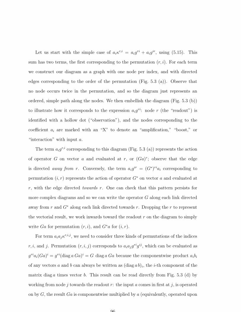
Let us start with the simple case of aiκr,i = aig

ri + aigir, using (5.15). This

sum has two terms, the first corresponding to the permutation (r, i). For each term

we construct our diagram as a graph with one node per index, and with directed

edges corresponding to the order of the permutation (Fig. 5.3 (a)). Observe that

no node occurs twice in the permutation, and so the diagram just represents an

ordered, simple path along the nodes. We then embellish the diagram (Fig. 5.3 (b))

to illustrate how it corresponds to the expression aigri: node r (the “readout”) is

identified with a hollow dot (“observation”), and the nodes corresponding to the

coefficient ai are marked with an “X” to denote an “amplification,” “boost,” or

“interaction” with input a.

The term aigr,i corresponding to this diagram (Fig. 5.3 (a)) represents the action

of operator G on vector a and evaluated at r, or (Ga)r; observe that the edge

is directed away from r. Conversely, the term aigir = (G∗)riai corresponding to

permutation (i, r) represents the action of operator G∗ on vector a and evaluated at

r, with the edge directed towards r. One can check that this pattern persists for

more complex diagrams and so we can write the operator G along each link directed

away from r and G∗ along each link directed towards r. Dropping the r to represent

the vectorial result, we work inwards toward the readout r on the diagram to simply

write Ga for permutation (r, i), and G∗a for (i, r).

For term aiajκr,i,j, we need to consider three kinds of permutations of the indices

r, i, and j. Permutation (r, i, j) corresponds to aiajgrigij, which can be evaluated as

griai(Ga)i = gri(diag a Ga)i = G diag a Ga because the componentwise product aibi

of any vectors a and b can always be written as (diag a b)i, the i-th component of the

matrix diag a times vector b. This result can be read directly from Fig. 5.3 (d) by

working from node j towards the readout r: the input a comes in first at j, is operated

on by G, the result Ga is componentwise multiplied by a (equivalently, operated upon

96

G*

r i

G

r ib:

a:

c: f:

e:

d:

G G

i

* *

G G

r

*

ijir

G G

r i j

jr

Figure 5.3: Diagrams for representing terms of the posterior mean (5.14). Eachdiagram corresponds to a particular permutation (via (5.15) for one of the terms.The permutation for each diagram is a: (r, i); b: (r, i); c: (i, r); d: (r, i, j); e: (j, i, r),and f: (j, r, i). The nodes represent indices in the term, and the edges represent theordering of indices in the corresponding permutation from the cirf cumulant. Thehollow nodes represent the output node (not summed over); the “X” indicates theapplication of an input a at the node.

by diag a), which is finally operated upon by G, to produce G diag a Ga. Since we

get the same diagram back when nodes i and j are swapped, to permutation (r, j, i)

we get the same result G diag a Ga. Permutation (j, i, r) has the diagram shown

Fig. 5.3 (e), which is the same as the reversal of the diagram for permutation (r, i, j),

and so corresponds to G∗ diag aG∗a. Again, nodes i and j can be swapped to produce

a G∗ diag aG∗a for permutation (i, j, r). The readout r need not be at the end of the

ordering, as in permutation (j, r, i) corresponding to term aiajgjrgri = (G∗a)r(Gr)r.

Letting a b denote the vector which is the componentwise product of vectors a and

b, i.e., (a b)i = aibi, the vector result from permutation (j, r, i) can therefore be

written as G∗a Ga := (G∗a) (Ga). This can also be derived from the diagram

97

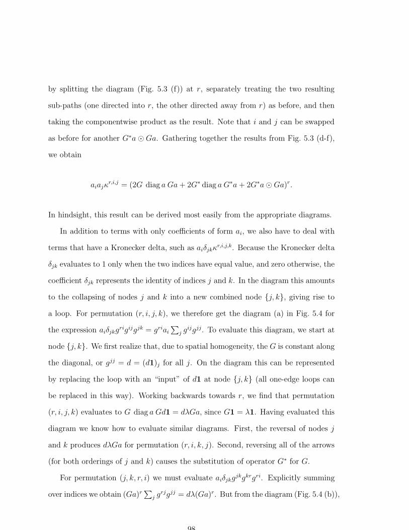
by splitting the diagram (Fig. 5.3 (f)) at r, separately treating the two resulting

sub-paths (one directed into r, the other directed away from r) as before, and then

taking the componentwise product as the result. Note that i and j can be swapped

as before for another G∗a Ga. Gathering together the results from Fig. 5.3 (d-f),

we obtain

aiajκr,i,j = (2G diag a Ga+ 2G∗ diag a G∗a + 2G∗aGa)r.

In hindsight, this result can be derived most easily from the appropriate diagrams.

In addition to terms with only coefficients of form ai, we also have to deal with

terms that have a Kronecker delta, such as aiδjkκr,i,j,k. Because the Kronecker delta

δjk evaluates to 1 only when the two indices have equal value, and zero otherwise, the

coefficient δjk represents the identity of indices j and k. In the diagram this amounts

to the collapsing of nodes j and k into a new combined node j, k, giving rise to

a loop. For permutation (r, i, j, k), we therefore get the diagram (a) in Fig. 5.4 for

the expression aiδjkgrigijgjk = griai

∑j g

ijgjj. To evaluate this diagram, we start at

node j, k. We first realize that, due to spatial homogeneity, the G is constant along

the diagonal, or gjj = d = (d1)j for all j. On the diagram this can be represented

by replacing the loop with an “input” of d1 at node j, k (all one-edge loops can

be replaced in this way). Working backwards towards r, we find that permutation

(r, i, j, k) evaluates to G diag a Gd1 = dλGa, since G1 = λ1. Having evaluated this

diagram we know how to evaluate similar diagrams. First, the reversal of nodes j

and k produces dλGa for permutation (r, i, k, j). Second, reversing all of the arrows

(for both orderings of j and k) causes the substitution of operator G∗ for G.

For permutation (j, k, r, i) we must evaluate aiδjkgjkgkrgri. Explicitly summing

over indices we obtain (Ga)r∑

j grjgjj = dλ(Ga)r. But from the diagram (Fig. 5.4 (b)),

98

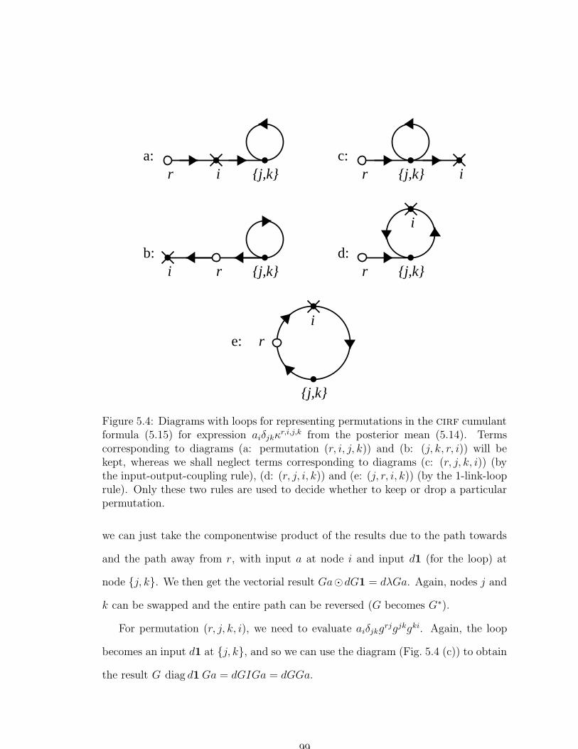
a:

b: d:

c:

j,ki j,k

i

r

j,k

i

r

e: r

r i j,k r ij,k

Figure 5.4: Diagrams with loops for representing permutations in the cirf cumulantformula (5.15) for expression aiδjkκ

r,i,j,k from the posterior mean (5.14). Termscorresponding to diagrams (a: permutation (r, i, j, k)) and (b: (j, k, r, i)) will bekept, whereas we shall neglect terms corresponding to diagrams (c: (r, j, k, i)) (bythe input-output-coupling rule), (d: (r, j, i, k)) and (e: (j, r, i, k)) (by the 1-link-looprule). Only these two rules are used to decide whether to keep or drop a particularpermutation.

we can just take the componentwise product of the results due to the path towards

and the path away from r, with input a at node i and input d1 (for the loop) at

node j, k. We then get the vectorial result GadG1 = dλGa. Again, nodes j and

k can be swapped and the entire path can be reversed (G becomes G∗).

For permutation (r, j, k, i), we need to evaluate aiδjkgrjgjkgki. Again, the loop

becomes an input d1 at j, k, and so we can use the diagram (Fig. 5.4 (c)) to obtain

the result G diag d1Ga = dGIGa = dGGa.

99

Now, observe that G is a positive operator for the Markov processes in which

we are interested8. Given that there is only one positive eigenvector for a positive

operator and that it corresponds to the maximum eigenvalue [55, p. 67], the equation

G1 = λ1 implies that λ is the maximum eigenvalue because 1 is a positive eigenvector

of G. This implies that λ−1G is a contraction mapping that only passes constant

vectors unchanged; non-constant vectors will shrink. Equivalently, ||Gy|| < ||λy||

unless y is a constant vector.

Because of this, we view the result dGGa = dGy for permutation (r, j, k, i) as

smaller than the result dλGa = dλy for permutation (j, k, r, i), where y = Ga is

generally non-constant for typical inputs a. Observe that such contraction mappings

will correspond to repeated operators (GG, G∗G∗, etc., without a “boost” or “am-

plification” from a between them) whenever there is a loop located between a regular

input a (located at i for permutation (r, j, k, i)) and the output r. As a first ap-

proximation, we shall therefore neglect dGGa and all other permutations that have

a Kronecker delta index between an input node and the output r; we shall restrict

our attention to those permutations where all of the indices with subscripted inputs

a form an uninterrupted sequence (in the permutation) to the output r. Let us call

this criterion for neglecting terms the input-output-coupling rule.

In addition to this rule for neglecting loops, there is another that is due to the ap-

proximately self-avoiding nature of our Markov processes. We illustrate this rule with

permutation (r, j, i, k) (Fig. 5.4(d)), or term aiδjkgrjgjigik =

∑j g

rj(Gji(G∗)ji)ai =

(G(GG∗)a)r, where AB denotes the componentwise product of the two operators

A and B. Here, the effective input at combined node j, k due to the 2-edge loop

j, k, i is (GG∗)a. We have “broken” the loop at i and taken the componentwise

8Equivalently, the Markov process on average spends nonzero time in every state j given that itstarted in state i, for both the direction and curvature processes; this can be seen from the plots ofthe Green’s operators, which—although they become very small—do not go exactly to zero awayfrom the impulse location (Figs. 2.2 and 2.4).

100

product of the operators that correspond to the two distinct paths from i to j, k;

this is the action of operator G G∗ on vector a. For approximately self-avoiding

processes, observe that GG∗ is approximately d2I: each row is the componentwise

product of the corresponding rows ofG and G∗, which, by spatial homogeneity, is just

the componentwise product of the Green’s operator kernels for the forward operator

G and the backward operator G∗. For the directed Markov process in 2 × , the

forward operator is large only on one side of the impulse, and the backward operator

is large only on the other, and thus the componentwise product is only significant

at the origin, which corresponds to the common diagonal gii = d. For the curvature

process in 2 × ×

, the forward and backward kernels may overlap for impulses

of high curvature, suggesting the need for a bound on curvature. Thus permutation

(r, j, i, k) evaluates to the simple expression d2Ga, which is clearly smaller than the

dλGa expression for permutation (r, i, j, k), since d = τ (the average amount of time

the contour spends in a site as it passes through) is certainly much less than the total

average contour length λ. This example suggests the 1-link-loop rule: neglect those

permutations that correspond to diagrams where the largest loop has more than one

link or edge.

5.6.5 Computational Significance of Approximately

Self-Avoiding Processes

It is interesting to note that for Brownian motion (a symmetric process, with G∗ = G)

there is perfect overlap between the forward and backward kernels, so the above

argument would not apply and therefore we should not invoke the 1-link-loop rule

to neglect such terms with inputs inside a loop. This suggests a novel justification

for orientation in vision: using approximately self-avoiding Markov processes (e.g.

101

the directed process in 2× ) gives rise to a reduction in computational complexity

compared to non-self-avoiding processes such as planar Brownian motion. Evolution

might exploit this fact since those organisms that expend fewer resources on contour

computations are more likely to survive. Observe that this is rather counter-intuitive

because it is the more elaborate representation ( 2 × ), not the simpler (

2), that

has the smaller computational burden. Also note that this complexity argument is

distinct from the statistical argument as to whether contours in the world do tend

to smoothly continue (§4.2) in orientation.

Returning to the calculation, both the 1-link-loop rule and the input-output-

coupling rule force us to drop permutation (r, j, i, k), but only the 1-link-loop rule

applies will cause us to neglect permutation (j, r, i, k) (Fig. 5.4 (e)). The latter

permutation, which has the output r within the loop can be evaluated by splitting

the loop at i, and then taking the componentwise product of the operators for the

two paths to the output r. Since there is no other loop at j, k, we view it as having

the input 1. (This evaluation of a loop at the output is only necessary if the output

is part of the loop.) The result is (GG∗G∗)a, which we assume to be small.

Bigger loops (with more inputs a) can be handled by breaking the loop at some

node and then forming the appropriate componentwise product operator, giving

rise to effective inputs (G diag a G) G∗a or G (G∗ diag a G∗ diag a G∗)a

at the combined node. Where there are loops within loops, we recursively evalu-

ate from the innermost loops by replacing each loop with the effective input at the

corresponding combined node and working toward the outermost loops. For the

purpose of evaluating the high-noise linear, quadratic, and cubic filters, the largest

loop will have only two internal inputs, corresponding to, for example, effective in-

puts (G diag a G) G∗a and its reversal G (G∗ diag a G∗)a. The use of

approximately self-avoiding processes will allow us to apply the 1-link-loop rule to

102

neglect these terms because, for example, each column of the “amplified” forward

operator G diag a G probably has little overlap with the corresponding column of

operator G∗. For filters of much higher-order than cubic, the 1-link-loop rule may

not be appropriate even for approximately self-avoiding processes because the ker-

nel for a long sequence of alternating forward operators and amplifications (e.g.,

G diag aG diag a · · ·G) may overlap with G∗; for example, a may represent an edge

map of a sufficiently smooth, closed contour.9 Again, we shall apply the 1-link-loop

rule for our cirf Volterra filters up to third order only.

More complicated diagrams than those above can arise; for example, there may

be no strict nesting of the loops. However, using the 1-link-loop rule we shall neglect

the terms corresponding to such diagrams. These more complex diagrams can rep-

resent highly improbable self-intersection patterns—tortuous paths—so neglecting

them seems reasonable.

In summary, we use a diagram-based technique for evaluating all the permutations

in the terms of the posterior mean expansion (5.14) for cirf linear, quadratic, and

cubic Volterra filters. We exploit the approximate self-avoidingness of our Markov

process G to invoke the 1-link-loop rule and the positivity of G for the input-output-

coupling rule. As a by-product we neglect a large variety of improbable looping

paths. We simplify our work by observing that we get the same diagram after

swapping indices in each Kronecker delta, and by implementing permutation reversals

by swapping G and G∗ appropriately. Unsuppressing η and the appropriate powers

of −12, this diagram-based calculation was used to derive the following.

Result 1 (High-noise MMSE CIRF Volterra Filters). Suppose that the curve

indicator random field U (for approximately self-avoiding Markov processes) is cor-

9For the direction process, if there is no diffusion in direction (σκ = 0) and space is unbounded,which corresponds to straight line trajectories, even higher-order kernels will never overlap.

103

rupted with additive Gaussian white noise of variance σ2N =: ε−1 to produce measure-

ment vector m. Let ζ := dλ, where d = gii and λ is the average curve length. Then

the minimum mean-squared error estimate of U given m has the following approxi-

mate asymptotic expansion as σN →∞ (ε→ 0):

Linear Filter:

u(1) = η1− 2εζ + ε(Gm +G∗m) +O(ηε2 + η2ε) (5.16)

Quadratic Filter:

u(2) = η1− 2εζ + 3ε2ζ2 + ε(1− 2εζ)(Gm+G∗m)

+ε2(G diagmGm +GmG∗m +G∗ diagmG∗m)

+O(ηε3 + η2ε) (5.17)

Cubic Filter:

u(3) = η1− 2εζ + 3ε2ζ2 − 4ε3ζ3

+ε(1− 2εζ + 3ε2ζ2)(Gm+G∗m)

+ε2(1− 2εζ)(G diagmGm+GmG∗m+G∗ diagmG∗m)

+ε3(G diagmG diagmGm+G diagmGmG∗m

+GmG∗ diagmG∗m+G∗ diagmG∗ diagmG∗m)

+O(ηε4 + η2ε). (5.18)

We shall see in Chapter 6 that by implementing the operator G in the Fourier

domain, its computational complexity is O(n logn) for the direction process, where

n = |I|. Since multiplying a diagonal matrix with a vector has O(n) complexity, the

104

net complexity for all of these filters is therefore O(n logn) for the direction process.

This is far better than for the general k-th order Volterra filters, which have O(nk+1)

complexity.

One could attempt to improve upon these results by pursuing higher-order ex-

pansions. However, instead of following that tedious, difficult path, we now turn to

a very different approach for deriving filters that is based on the mgf of the cirf

that we derived in Chapter 3. Unlike for general signals, we can follow this path due

to the special structure of the cirf. Not only is the approach simpler, it also allows

one to exploit all of the probabilistic structure in the cirf.

5.7 The Biased CIRF Approximation

of the Posterior

In addition to deriving high-noise Volterra filters by using the low-order cumulants

of the prior, we can also compute filters by approximating the posterior with a more

manageable distribution. This idea has found numerous applications in Markov

random fields, Boltzmann machines, and recurrent neural networks, where a highly

coupled system is approximated with completely uncoupled system that is trivial to

handle [91]. A common theme in those approximations is that the random influences

on a site are replaced with their average, giving rise to a coupled system of equa-

tions in the unknown means. Inspired by its original application in statistical field

theory [90], this procedure is known as the mean-field approximation. More recent

presentations of mean-field approximation seek to minimize the Kullback divergence

between a given distribution and its approximation by taking a perturbation expan-

sion to a factored distribution [106, 53, 114, 115]. We shall now develop a related

approximation for the cirf, although the approximation will not be factored.

105

Because by Bayes’ rule any posterior is a weighted version of the prior, it is

reasonable to base our approximation on the prior. Although the prior itself will not

suffice as an approximation, since it is not even a function of the measurements, the

prior can be modified or “biased” by a function of the measurements to make a useful

approximation of the posterior. To see how to do this, recall from §3.4.2 that we have

a tractable expression for the cirf moment generating functional

exp〈c, U〉, where

the moments are obtained by differentiating the mgf and evaluating the derivatives at

c = 0. However, the mgf of the cirf converges for all c sufficiently small (Prop. 3),

and so we could evaluate the derivatives at c 6= 0, i.e., perform a Taylor series

expansion around c 6= 0. Doing so amounts to finding the moments of a cirf of bias

c, or biased cirf, with distribution Pc(du) := Z−1c exp〈c, u〉P (du), where c ∈ |I|

is the bias (vector), P (du) is the original (unbiased) cirf distribution, and Zc :=

∫exp〈c, u〉P (du). Expectations with respect to Pc are indicated with

c. We shall

first compute the cumulants of the biased cirf and then set up a system of equations

that allows us to approximate the true posterior with a biased cirf. All statistics of

the posterior can then be approximated by those of the approximating biased cirf

distribution. In particular, the posterior mean of the cirf can be approximated in

this way.

5.7.1 Cumulants of the Biased CIRF

To compute the cumulants of the biased cirf we need to take derivatives of its

cumulant generating functional ln

c exp〈b, U〉 with respect to the vector b, and then

evaluate them at 0. Since cgfc(b) := ln

c exp〈b, U〉 = ln∫

exp〈b+c, u〉P (du)−lnZc,

taking derivatives with respect to b of the cgf of the biased cirf (denoted cgfc(b))

and evaluating at 0 is equivalent to taking derivatives with respect to c of the cgf

ln

exp〈c, U〉 of the (unbiased) cirf and evaluating at c.

106

For example, to compute the mean of a biased cirf, we have to compute

∇c ln

exp〈c, U〉 =

(∂

∂c1ln

exp〈c, U〉, . . . , ∂

∂c|I|ln

exp〈c, U〉

),

where ∇c denotes the gradient with respect to c. Substituting the cirf moment

generating functional (Prop. 5), we have to take the gradient of 〈µ, N (Gc −G)ν〉 =

N [〈µ,Gcν〉−1], where we recall the notationGc := G(c) for the Green’s operator with

bias c. Applying the gradient to the latter inner product, we can write ∇c〈µ,Gcν〉 =

〈µ, [∇cGc]ν〉.

Since Gc := −(Q+diag c)−1, to continue the calculation we must understand how

to take derivatives of inverses of operators, which we study in the following lemma.

Lemma 4. Suppose matrices A = (aij) and B = (bij) are functions of some pa-

rameter α, i.e., A = A(α), B = B(α). Letting primes ( ′) denote (componentwise)

derivatives d/dα with respect to α, the following formulas hold:

(AB)′ = A′B + AB′, (5.19)

(A−1)′ = −A−1A′A−1. (5.20)

proof. Formula (5.19) follows by applying the single variable product rule to the

sum from the inner product of a row of A and column of B: (AB)′ij = (∑

k aikbkj)′ =

∑k(a

′ikbkj + aikb

′kj) = (A′B + AB′)ij.

To obtain formula (5.20), we first apply formula (5.19) to write 0 = I ′ =

(AA−1)′ = A′A−1 + AA−1′. Then we solve for A−1′.

Returning to the calculation of the mean of the biased cirf, we use (5.20) to write

∂∂ciGc = ∂

∂ci[−(Q + diag c)−1] = (Q + diag c)−1

[∂

∂ci(Q + diag c)

](Q + diag c)−1 =

GcDiGc, where Di is a matrix with a one at the (i, i)-entry and zeroes elsewhere. The

107

matrix Di can be expressed as the outer product δiδ∗i of discrete impulse vectors δi

at site i, where (δi)j = δij. Therefore ∂∂ci〈µ,Gcν〉 = (δ∗iG

∗cµ) (δ∗iGcν) = (G∗

cµ)i(Gcν)i,

proving the following:

Proposition 7. The mean of the cirf of bias c at site i is

κic =

cUi = N 〈µ,GcDiGcν〉. (5.21)

Equivalently, the mean (vector) of this biased cirf is

cU = N (G∗

cµ) (Gcν). (5.22)

The higher-order cumulants can also be tractably characterized as follows:

Proposition 8. The k-th cumulant at sites i1, . . . , ik of the cirf U of bias c is

κi1,...,ikc = cumcUi1 , . . . , Uik = N 〈µ,

∑

a∈permk

GcDia1Gc · · ·GcDiak

Gcν〉 (5.23)

= N∑

i,j

µiνj

∑

a∈permk

giia1c g

ia1ia2c · · · giak−1

iakc g

iakj

c ,

where (gijc ) := Gc is the Markov process Green’s operator with bias c.

proof. Since by definition cumcUi1, . . . , Uik = ∂k

∂ci1···∂cik

(N 〈µ,Gcν〉−N ), we need

to show

∂kGc

∂ci1 · · ·∂cik=

∑

a∈permk

GcDia1Gc · · ·GcDiak

Gc. (5.24)

(Here and in the following, all derivatives will be evaluated at c.) We shall prove

(5.24) by induction. By the proof of Prop. 7, formula (5.24) holds for k = 1. Suppose

108

(5.24) holds for k = n. We now check the case k = n+ 1:

∂n+1Gc

∂ci1 · · ·∂cin+1

=∂

∂cin+1

∑

a∈permn

GcDia1Gc · · ·GcDian

Gc

=n+1∑

j=1

∑

a∈permn

GcDia1Gc · · ·GcDiaj−1

(GcDin+1Gc)DiajGc · · ·GcDian

Gc

=∑

a∈permn+1

GcDia1Gc · · ·GcDian+1

Gc,

using ∂Gc

∂ci= GcDiGc from the proof of (5.21) again. The result follows.

5.7.2 Solving for the Biased CIRF

Given this manageable characterization of the cumulants of the biased cirf, our task

now is to solve for the bias c to approximate the posterior. Because the logarithm

lnZ(ε) of the normalizing constant Z(ε) of the posterior is (up to an additive constant)

just the cumulant generating functional of the posterior (see §5.7.1), we shall develop

an approximation to lnZ(ε). The general strategy is similar to that for the Volterra

filter, where we assume there is high-noise (ε near 0), and so a perturbation expansion

in ε is warranted. Except in the sense of the remainder term of the expansion, we do

not provide approximation bounds10. Letting εc′ = c, we write

lnZ(ε) = ln

∫eε〈a+Au,u〉 P (du)

= ln

∫eε〈a−c′+Au,u〉 eε〈c′,u〉 P (du)

= lnZεc′

εc′ eε〈a−c′+AU,U〉

= lnZc + ln

c eε〈a−c′+AU,U〉, (5.25)

10Approximation bounds for sigmoidal belief networks are provided in [106].

109

where the second term on the last line is simply the cumulant generating functional

of 〈a− c′ +AU,U〉 (with respect to measure Pc(du)) evaluated at ε, similar to (5.11)

except the measure on U is now biased by c. Now, as for the Volterra filters, we shall

develop the cgf of 〈a−c′+AU,U〉 into a Taylor series in ε. Unlike the Volterra case,

however, we have the extra freedom to choose the bias c to make our approximation

useful, and therefore we shall stop the Taylor series at the first order, i.e.,

ln

c eε〈a−c′+AU,U〉 = ln(1 +ε〈a− c′ +AU,U〉+O(ε2 =

cε〈a− c′ +AU,U〉+O(ε2).

Because the latter expectation is just −〈c, cU〉 + ε〈a,

cU〉 + ε∑

j

c[(AU)jUj], we

can rewrite (5.25) as

lnZ(ε) = lnZc−〈c,

cU〉+ε〈a,

cU〉+∑

j

[covc((AU)j, Uj) +

c(AU)j

cUj]

+O(ε2).

(5.26)

Since lnZ(ε), which characterizes the true posterior, does not depend on the bias c

of our approximate posterior Pc, differentiating lnZ(ε) with respect to any function

of c will be zero. In particular, we can set up a system of equations in c by taking

the derivative of (5.26) with respect to

cUi = κic, a function of c. We consider two

special cases now.

No Blur Case

Consider the situation where there is no blur in the observations and the noise is

white. Thus we set A = − 12I = −1

2(δij) and (5.26) becomes

lnZ(ε) = lnZc −∑

j

cjκjc + ε

∑

j

ajκjc −

1

2

∑

j

[κj,j

c + κjcκ

jc

]

+O(ε2). (5.27)

110

Differentiating with respect to κic and applying the chain rule twice, the first two

terms on the right hand side become

∂

∂κic

[lnZc −

∑

j

cjκjc

]=∑

j

∂ lnZc

∂cj

∂cj∂κi

c

− ci −∑

j

∂cj∂κi

c

κjc = −ci, (5.28)

because ∂ lnZc

∂cj= κj

c. Using formula (5.23) twice, note that κjjc = 2gjj

c N∑

i′,j′ µi′νj′gi′jc gjj′

c =

2gjjc κ

jc, because the two permutations are identical. So by differentiating (5.26) with

respect to κic, we get: 0 = −ci + ε(ai − gii

c +

cUi) + O(ε2), proving the following

result:

Result 2. Suppose the posterior distribution of the observed cirf is P(ε)(du) ∝

exp(ε〈a− 12u, u〉)P (du). Then P(ε) can be approximated by a cirf of bias c, with

c = ε[a− cU − d(c)] +O(ε2), (5.29)

where d(c) is the diagonal of the Green’s operator Gc with bias c, or d(c)i := giic .

As discussed in §5.2.1, we can apply this result to the case where the cirf is

corrupted with additive Gaussian white noise by setting a = m and ε = σ−2N . This

can also be applied when empirical edge histograms are known (§5.2.3) or in other

situations by setting a to an appropriate function of m.

Observe that (5.29) is a coupled nonlinear system in the vector c of |I| unknowns;

c is expressed as a function not only of the exogenous a, but also of the (generally

nonlinear) functions of itself:

cU (see Proposition 7) and d(c). This equation de-

scribes c as proportional to a balance between positive influence due to input a and

negative influence due to the sum of the mean of the biased cirf (

cU) and a mea-

sure of closure d(c). Recall that d(c)i = (Gc)ii is the expected amount of time that

the biased Markov process spends in site i given that it started at i. We note that

111

even if the unbiased process is self-avoiding, the bias may be such as to encourage

the process to return to i. In the context of Mumford’s direction process, if c is

sufficiently positive along an appropriate dilation of a smooth closed curve passing

through i in discrete 2× , then d(c)i may be large. This closure measure may not

be significant if the bias describes only open curves. Since the bias c is ultimately a

function of input a, we would expect d(c) to be important only when a is positive

along smooth, closed curves.11

Large Blur Case

Another system of equations can be derived in an opposite extreme, where the sym-

metric negative definite matrix A is proportional to an operator that performs a

great deal of blur. In that case, the blurred field AU is essentially a constant vector,

and therefore covc((AU)j, Uj) ≈ 0. Using ∇ cU〈

cAU,

cU〉 = 2A

cU and the above

calculations for the no-blur case, we get the following system of equations.

Result 3. Suppose the posterior distribution of the observed cirf is P(ε)(du) ∝

exp(ε〈a+ Au, u〉)P (du), where the symmetric negative definite operator A is approx-

imately proportional to a spatial averaging operator of maximum size, such as a

matrix of constants. Then P(ε) can be approximated by a cirf of bias c, with

c ≈ ε[a + 2A

cU ] +O(ε2). (5.30)

This large blur result provides a nonlinear system of equations in the bias c. It

differs from (5.29) by the presence of the blur operator A acting on the mean and

11The exact notion of smoothness and closedness will depend on the Markov process curve model.For the direction process, closed curves with curvature not many times that of σκ might induce ad(c) having large values at some sites.

112

the absence of the closure measure d(c). By including blur, we can better describe a

number of situations, as outlined in §5.2

Also note that for both the non-blur and large blur cases, the biased cirf approx-

imations do not depend on a spatial homogeneity assumption, and so nonuniform µ

and ν can be used.

Combined with the formula for the mean of the biased cirf and dropping terms

of order ε2, our nonlinear system corresponding to (5.30) can be expressed as the

following coupled nonlinear system describing a self-consistent field c mediating the

posterior cirf interactions:

Observation (Biased CIRF Approximation of the Posterior Mean of the

CIRF). Suppose a cirf U is corrupted via a quadratic log-likelihood (with large-

scale blur) to produce measurements m. The posterior mean of U given m has the

following approximate description:

mU ≈ N f b, (5.31)

where f and b solve the following coupled system:

Qf + ε diag[a + 2NA(f b)]f + ν = 0 (5.32)

Q∗b+ ε diag[a + 2NA(f b)]b + µ = 0. (5.33)

For reference, we include the above filtering equations for the continuum-limit of

the above biased cirf approximation equations for the direction process.

Observation (Reaction-Diffusion-Convection Equation for the Direction

Process). Suppose a cirf U based on the direction process is corrupted via a quadratic

log-likelihood (with large-scale blur) to produce measurements m. Then the posterior

113

mean is approximately N f b, where f and b solve the following coupled nonlinear

integro-elliptic system:

(σ2

2

∂2

∂θ2− cos θ

∂

∂x− sin θ

∂

∂y− α

)f + ε diag[a + 2NA(f b)]f + ν = 0

(σ2

2

∂2

∂θ2+ cos θ

∂

∂x+ sin θ

∂

∂y− α

)b + ε diag[a + 2NA(f b)]b + µ = 0.

Also note that for A, the nonlinear coupled pde is in fact a reaction-diffusion-

convection equation. Since c ≈ ε[a + 2NA(f b)], we see that pattern formation

arises from c+ = max(c, 0) (the positive part of bias c), pattern repression comes from

−c− = min(c, 0) (the negative part of c), diffusion comes from the second derivatives,

and convection is due to the first derivatives [136].

5.8 Comparison with Completion Fields

Perceptual organization has tantalized a number of researchers in computer vision

with the possibility of discovering a rigorous foundation for classical demonstrations

such as illusory contours [52]. This gave rise to work on contour saliency both as a

model of illusory contour formation and for contour organization. We shall focus on

drawing relationships to stochastic completion fields [126, 109] and eigensources [117]

because of their focus on Markov processes such as the direction process. Stochastic

completion fields in particular were a strong inspiration for this thesis.

To make the connection, we begin with the biased cirf approximation, but set the

operator A to zero. The first consequence of dropping A is that the likelihood is no

longer necessarily normalizable. For the second consequence, recall the interpretation

of the square of the cirf U as a measure of contour intersections (see §3.1.1). Ignoring

the operator A (which gives rise to a quadratic form in U) therefore amounts to

114

ignoring those intersections (due to the diagonal of A) or even near intersections (due

to the off-diagonals of A). With this simplification this biased cirf approximation

becomes the decoupled forward and backward linear systems Qf + Cf + ν = 0 and

Q∗b+Cb+µ = 0, respectively, where C := ε diag a. The approximate posterior mean

of the cirf U is proportional to the componentwise product fb of the forward and

backward solutions. We focus on the forward equation, as the backward equation is

just its adjoint.

Now, we observe even though we have dropped the interaction operator A, the

resulting filter is still a nonlinear input-to-output mapping, and in two distinct ways.

First, we are taking the product of the forward and backward solutions. Second, the

input arises as a modification to the diagonal of linear operator Q. In particular,

we have f = (I − GC)−1Gν =∑∞

k=0(GC)kGν, which says that f is an infinite

polynomial in c, i.e., f is nonlinear in c. If we ignore the constant term (k = 0)

and all nonlinear terms (k > 1), what remains is the linear term GCGν, which

is proportional to Gc if ν is a constant vector and G is spatially homogeneous (as

it is for the direction process). We recognize Gc as the source field (with sources

c ∝ CGν), and, by the same argument, G∗c is the sink field (with sinks c ∝ CG∗µ,

where µ is also a constant vector); their product Gc G∗c is then Williams’ and

Jacobs’ stochastic completion field [126]. To have different sinks and sources one can

adjust µ and ν.

To relate to eigensources, let C := diag a and thus write the forward equation

as: f − εGCf − Gν = 0. Setting ν = 0 and assuming ai > 0, for all i, we can

define W 2 := C to get GW 2f = σ2Nf, where we recall ε = σ−2

N (see §5.2.2). Defining

h = Wf , we write GWh = σ2NW

−1h, or

WGWh = σ2Nh.

115

This is an eigenvalue equation of the same form as in [117], where σ2N is now in-

terpreted as an eigenvalue of WGW . We see, therefore, that the cirf provides a

new perspective for understanding other techniques for the perceptual organization

of contours.

5.9 What Can One Do with a Filtered CIRF?

It may seem odd that we have sought to (merely) filter a field of local contour

measurements, producing yet another field. If one objective of vision is to explicitly

represent structures with increasing abstraction, this task may seem to postpone the

most difficult work. To return to a question brought up at the start of this chapter,

why not extract the contours directly from the image, instead of just enhancing a

contour image?

There are a number of reasons why one might focus on processing a field. First,

this approach captures a notion of global information beyond that of a single curve,

by explicitly expressing the idea of an image of contours, where both the inter-

actions among the contours and the blur due to imaging is not ignored. In con-

trast, previous approaches for computing curves using Markov process contour mod-

els [80, 108, 35, 15, 26, 126, 133], implicitly assume that there is only a single contour.

By emphasizing the field we can combine the richer contour models of the single-

contour schemes with the contour interactions implicit in the line processes used in

mrfs [36] or dictionary-based relaxation labeling [40]. Another reason for the inter-

mediate representation of a filtered cirf is that it captures the ambiguity inherent

in finding contours in noisy images: a more diffuse filter response characterizes less

certain (more spread out) contours. If direct contour computations were carried out,

one would need a set of contours to represent this ambiguity. While in some appli-

116

cations only the best contour is needed, in others we require an assessment of the

uncertainty of the situation and some representation of the plurality of comparable

contour explanations.12 Direct enumeration with particular contours may be more

cumbersome than a field for representing the many contour possibilities. Finally,

contour enhancement can be an end in itself in some graphical or image processing

applications.

More pragmatically, simple post-processing of the filtered cirf may be sufficient

for some applications. For example, the thresholding described in §5.1.4 may be

sufficient, perhaps followed by connected component analysis (in 3-d for the directed

Mumford process, for example) to provide a thick individual contours, providing a

description qualitatively similar to Iverson’s thick trace [49]. Thinning and linking

procedures could then follow if desired.

Since information is lost in thresholding, however, for more sophisticated con-

tour processing, might require the (un-thresholded) cirf posterior mean. To com-

pute contours one could greedily follow gradients in the posterior mean from strong,

supra-threshold seed points. The cirf posterior mean could also be used to guide

a heuristic search procedure for finding individual contours [73]. Since the (filtered)

cirf is the expected amount of time a contour spends at a site (given the measure-

ments), the posterior mean is a candidate heuristic function that would encourage

sites with large times to be explored first and more often than others. Other graph-

based methods [12] could be used to post-process the cirf in a similar fashion. By

combining information about the observation process and the structure of contours,

the cirf performs significant global computations, and so reduces the burden upon

later processing.

12See [116] for explicit calculations of such contour diffusivity.

117

Chapter 6

Numerical Methods

Having worked out formulas for mmse cirf filters, we now discuss how these can

be implemented. While the number of linear and nonlinear filters we have suggested

may seem daunting, on closer inspection of the formulas in Chapter 5 we see some

common components. For example, the Green’s operatorG for the generator L of the

Markov process appears in the linear and Volterra filters. In addition, the Green’s

operator Gc of the biased cirf also appears prominently in filters based on the biased

cirf approximation of the cirf posterior. We therefore first study the problem of

computing the action f = Gh of G upon h for both the direction and curvature

processes, where in both cases we have direct (noniterative) methods. Knowing how

to applyG to a vector enables us to compute the action of the biased Green’s operator

Gc on a vector using an iterative technique that uses G as a preconditioner. The

technique for computing Gc does not itself depend upon the Markov process because

those details are summarized by G. Finally, we present a continuation method for

solving the nonlinear system for the biased cirf. The continuation method requires

that we be able to apply Gc, and so it is also not tied to a particular Markov process.

118

6.1 Applying the Green’s Operator by Solving the

Forward Equation

To compute the action f of the Green’s operator G upon a vector h, we can—

equivalently—solve for f in the forward equation

(αI − L)f = h, (6.1)

since Q = L − αI and G = −Q−1. Now, all of the theory in Chapters 3 and 5 was

based on continuous-time, discrete-space Markov processes, to avoid many measure-

theoretic distractions. However, as we saw in Chapter 2, the Markov processes we

are most interested in live in continuous spaces such as 2 × . In general, by de-

signing a Markov process via an appropriate stochastic differential equation, we can

immediately obtain the process’s generator L from the corresponding Fokker-Planck

equation. When the Markov process is a diffusion process, L is a partial differential

operator acting on functions of continuous space, not vectors. To make the tran-

sition from the continuous to discrete domains, we let the discrete-space generator

L be some (reasonable) discretization of the continuous-space generator L. Strictly

speaking, therefore, the cirf filters are only fully defined when we specify the nu-

merical method used to obtain a particular (discrete) generator L. We discretize

only after having studied the filtering problem to focus on the underlying mathe-

matics of filtering curve images, not the (often crucial) details of implementation.

By this thinking, we may imagine that our filters require the solution of differential

or integral equations, even though we only solve their discretizations. In addition,

although we employ particular numerical techniques here, we note that they are not

unique, as in many numerical problems.

119

6.1.1 Direction Process

Here we solve the (discrete) forward equation for Mumford’s direction process by

first specifying the related direction process forward pde and then discretizing using

Fourier series. The result will be a set of linear systems in the frequency domain that

can be solved rapidly. After taking an inverse discrete Fourier transform, we shall

find that we can accurately compute the action f = Gh of G on a vector h ∈ n

in O(n logn)-time. Because this technique does not require iteration, we call it the

direct method.

Recalling the continuous-space generator L of the direction process from (2.4),

the corresponding forward pde is the continuous space equivalent (αI − L)f = g of

(6.1), or the direction process forward pde

αf − σ2

2

∂2f

∂θ2+ cos θ

∂f

∂x+ sin θ

∂f

∂y= h, (6.2)

where f = f(x, y, θ), h = h(x, y, θ), and σ = σκ > 0. Observe that this is a

degenerate elliptic pde, where the degeneracy arises because the second derivatives

do not appear in x and y. As Mumford [82] and later Williams and Jacobs [125] have

noted for the corresponding Fokker-Planck diffusion equation, the second derivative

in θ gives rise to diffusion in the θ-dimension, and the cosine/sine pair of terms

give rise to convection. Suppose we are to solve (6.2) on D × [0, 2π], for planar

rectangular region D = [0, xmax] × [0, ymax] ⊂ 2. Let ∂D denote the boundary of

D. For boundary conditions, we always assume f(x, y, θ) is periodic in θ with period

2π. With respect to (x, y), one may study several possible boundary conditions:

• Dirichlet: f(∂D, θ) = 0, ∀θ;

• Neumann: ∂f∂n

(∂D, θ) = 0, ∀θ, where n is the outward normal of D;

120

• Periodic: f is periodic in x with period xmax and in y with period ymax.

The Dirichlet and Neumann boundary conditions may be more natural for contour

enhancement, as periodic boundary conditions can lead to “wrap around” artifacts.

At least two major approaches can be taken in numerically solving pde (6.2): (1)

finite differencing, or (2) projection onto another basis. In the first approach, the par-

tial derivatives are replaced with (discrete) difference approximations, similar to the

definition of a derivative except without taking the limit. Finite differencing not only

is simple to implement, but it also allows boundary conditions to be easily specified

and modified. Williams and Jacobs used finite differencing to solve the corresponding

time-dependent Fokker-Planck pde (with decay), where the approximation was only

first-order accurate because upwind differencing was needed for stability [125]. They

observed a troubling anisotropy with this first-order method: the solution is more

focused in the horizontal and vertical directions than in the diagonals (see Fig. 6.1).

In other words, rotating h does not simply rotate the solution f , as pde (6.2) would

predict. Extra diffusion was later added to restore isotropy [127], with the additional

benefit of enabling a fast multi-grid solution. Unfortunately, this technique ensured

that all directions had the same unfocused response as the diagonals did without ex-

tra diffusion. It has been difficult to achieve accuracy in solving the direction process

forward pde while maintaining isotropy using finite differencing.

A second approach to solving the direction process forward pde (6.2) involves

selecting a suitable (and typically orthogonal) basis φk, taking the inner prod-

uct 〈φ, ψ〉R :=∫φ(r)ψ∗(r) dr (where the asterisk denotes complex conjugation,

r = (x, y, θ) ∈ R = 2 × ,, and the subscript R is dropped if understood from

the context) of the equation with the basis elements, and then solving the trans-

formed system. A judicious selection of basis can lead to reduced computation

times and/or solution quality. One important virtue of the complex exponential

121

(or complex Fourier) basis is that derivatives can be represented exactly by scalar

multiplication, suggesting that the anisotropy introduced by finite differencing might

be alleviated. In addition, the ready availability of reliable implementations of the

fast Fourier transform (fft), which compute the projection to the complex expo-

nential basis, make coding straightforward. Finally, we shall see that pde (6.2)

reduces to a set of cyclic tridiagonal systems, which can be rapidly solved. Zweck

and Williams solved the related time-dependent diffusion equation by projecting

onto localized wavelet-like bases and obtained superb isotropic performance; unfor-

tunately, the computational cost of their scheme is greater than the cost of finite

differencing [140]. The need to apply the Green’s operator possibly many times to

implement our mmse filters motivated us to devise the following rapid scheme.

Before developing our method, we observe that trigonometric bases correspond

to the three different boundary conditions. Specifically, the sine, cosine, and com-

plex exponential bases correspond to the Dirichlet, Neumann, and periodic boundary

conditions respectively. Despite the periodicity of the complex exponential basis, we

apply it here both because of the above advantages and to simplify the presentation.

To reduce the negative artifacts of periodicity in (x, y), we can often solve the equa-

tion on a larger domain than necessary (after suitably padding h), and then extract

the region of interest from the solution f .

We now detail our direct method. Letdenote the imaginary unit

√−1. The com-

plex exponential having periods xmax, ymax, and 2π and at frequencies j, k, and l in the

x-, y-, and θ-dimensions, respectively, is φjkl(x, y, θ) := exp[2π

( jxxmax

+ kyymax

+ lθ2π

)].

Let the Fourier coefficient fjkl be defined as the inner product 〈f, φjkl〉 of a function

f with a complex exponential φjkl; hjkl is defined similarly. Now we can evalu-

ate, term-by-term, the inner product of the complex exponential with the direction

process forward pde.

122

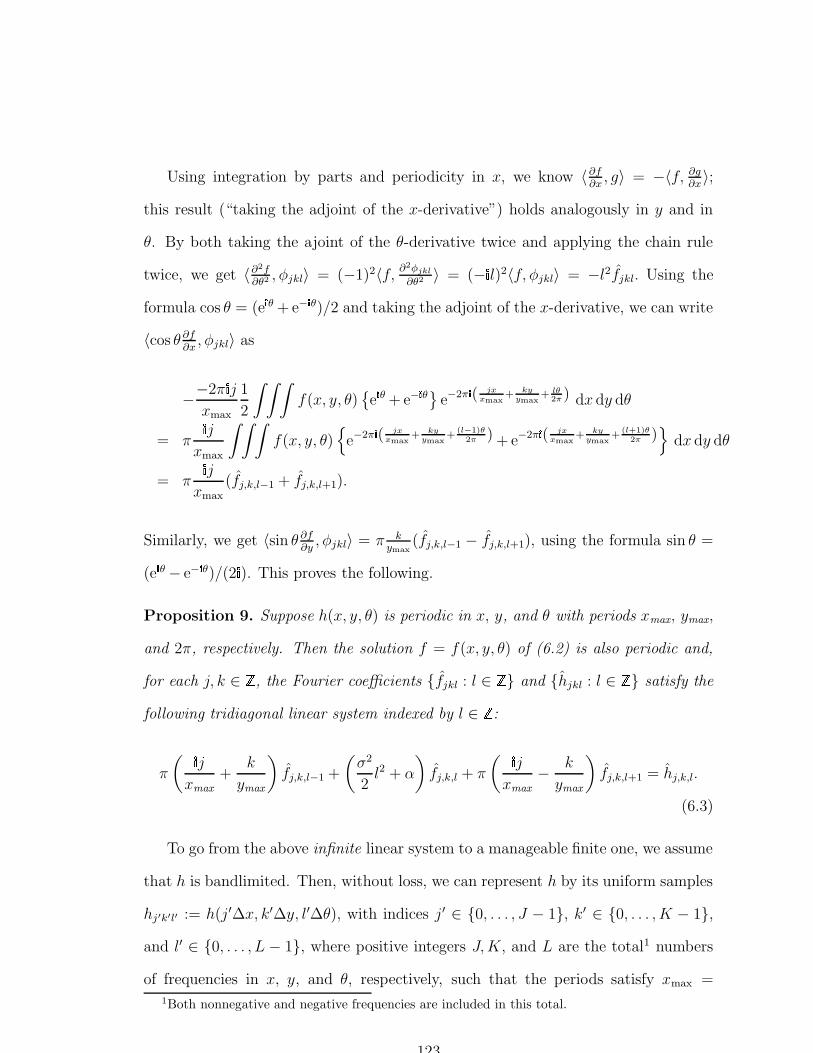
Using integration by parts and periodicity in x, we know 〈 ∂f∂x, g〉 = −〈f, ∂g

∂x〉;

this result (“taking the adjoint of the x-derivative”) holds analogously in y and in

θ. By both taking the ajoint of the θ-derivative twice and applying the chain rule

twice, we get 〈∂2f∂θ2 , φjkl〉 = (−1)2〈f, ∂2φjkl

∂θ2 〉 = (− l)2〈f, φjkl〉 = −l2fjkl. Using the

formula cos θ = (eθ + e−

θ)/2 and taking the adjoint of the x-derivative, we can write

〈cos θ ∂f∂x, φjkl〉 as

−−2πj

xmax

1

2

∫ ∫ ∫f(x, y, θ)

e

θ + e−

θ

e−2π( jx

xmax+ ky

ymax+ lθ

2π ) dx dy dθ

= π

j

xmax

∫ ∫ ∫f(x, y, θ)

e−2π

( jx

xmax+ ky

ymax+ (l−1)θ

2π ) + e−2π( jx

xmax+ ky

ymax+ (l+1)θ

2π )

dx dy dθ

= π

j

xmax

(fj,k,l−1 + fj,k,l+1).

Similarly, we get 〈sin θ ∂f∂y, φjkl〉 = π k

ymax(fj,k,l−1 − fj,k,l+1), using the formula sin θ =

(eθ − e−

θ)/(2

). This proves the following.

Proposition 9. Suppose h(x, y, θ) is periodic in x, y, and θ with periods xmax

, ymax

,

and 2π, respectively. Then the solution f = f(x, y, θ) of (6.2) is also periodic and,

for each j, k ∈ , the Fourier coefficients fjkl : l ∈ and hjkl : l ∈ satisfy the

following tridiagonal linear system indexed by l ∈ :

π

( j

xmax

+k

ymax

)fj,k,l−1 +

(σ2

2l2 + α

)fj,k,l + π

( j

xmax

− k

ymax

)fj,k,l+1 = hj,k,l.

(6.3)

To go from the above infinite linear system to a manageable finite one, we assume

that h is bandlimited. Then, without loss, we can represent h by its uniform samples

hj′k′l′ := h(j ′∆x, k′∆y, l′∆θ), with indices j ′ ∈ 0, . . . , J − 1, k′ ∈ 0, . . . , K − 1,

and l′ ∈ 0, . . . , L − 1, where positive integers J,K, and L are the total1 numbers

of frequencies in x, y, and θ, respectively, such that the periods satisfy xmax =1Both nonnegative and negative frequencies are included in this total.

123

J∆x, ymax = K∆y, and 2π = L∆θ. Prop. 9 then implies f is bandlimited in x

and y. Due to the bandlimitedness of h in θ and the fact that the direction process

forward pde is a diffusion in θ (and thus low-pass), we elect to solve for f in (6.3)

only for the same L total frequencies in θ that are in the bandlimit of h. To deal

with the “boundary conditions” in frequency l, we assume that fjkl is periodic in

l because sampled signals have periodic spectra.2 As a result, we obtain an L × L

cyclic tridiagonal linear system at each (j, k) frequency pair. Assuming L is even,

this sytem is Afj,k,· = hj,k,·, where the matrix A is:

γ−L/2+1 β− 0 · · · · · · 0 β+

β+ . . .. . .

. . . 0

0. . . γ−1 β− 0

...

.... . . β+ γ0 β−

. . ....

... 0 β+ γ1. . . 0

0. . .

. . .. . . β−

β− 0 · · · · · · 0 β+ γL/2

, (6.4)

where γl = σ2

2l2 + α, β+ = π

( j

J∆x+ k

K∆y

), and β− = π

( j

J∆x− k

K∆y

). This system

can be solved for fj,k,· in O(L) operations [96]. Using the fft to compute the (finite

number of) Fourier coefficients of h and the inverse fft to compute f from f , the

overall time complexity of computing f from h is O(n logn), where n = J ·K · L.

When the input—before discretization—is not bandlimited, aliasing and oscil-

lation can occur both in the (discrete) input and solution. For example, if the

discretization of h is a discrete impulse (a “1” at one position, with “0”s else-

where), the corresponding continuous-space h is not a Dirac δ-distribution, since

2Periodic boundary conditions in l produced more pleasing results than zero boundary conditionsin an informal test where the θ-dimension was badly undersampled. If the θ-dimension is sufficientlyoversampled, the difference is negligible.

124

the δ-distribution is not band-limited. Instead, the continuous-space h correspond-

ing to a discrete impulse is a sinc function3 centered on the impulse and with zero

crossings at all other sample locations. Between the sample locations the sinc oscil-

lates above and below zero. If the discrete impulse is shifted by a non-integral number

of samples, which can only fairly mean that the underlying continuous signal—the

sinc function—is so shifted and then resampled, the discretization will no longer be a

discrete impulse, but will have (discrete) oscillations. This phenomenon also appears

in the solution of the direction process forward pde (Fig. 6.2).

The corresponding backward equation (αI−L∗)f = h requires taking the adjoint

of the direction process generator, which in this case amounts to flipping the signs

on the first derivatives. Obeying these sign changes, the backward equations can be

solved similarly.

Instead of numerically solving the direction process forward pde, one can also

compute the action f = Gh by particle simulation [126]. This technique amounts to

the estimation of the integral kernel g(x0, y0, θ0; x1, y1, θ1) for the continuous-space

operator G (used to idealize G = (gij)) directly by simulating a large number of

particles behaving as the direction process, and then taking advantage of the in-

terpretation that gij is the average amount of time the particles spent in location

j, given that they started at i, where i and j are discrete-space approximations of

(x0, y0, θ0) and (x1, y1, θ1), respectively. Error will be introduced both in the time

discretization required to track the individual particles on a digital computer and in

the spatial discretization of the Markov process. The action f = Gh can be com-

puted by explicit integration, leading to an O(n2)-time computation. Not only are

such integrations expensive, the particle simulations can be as well (to ensure that

3The (standard) sinc function has a period of infinity. For finite periods, qualitatively similarfunctions arise.

125

the averages have low variance4). To avoid the error due to the finite number of par-

ticles, Thornber and Williams also set up related diffusion processes in direction and

scale for which convenient approximate formulas for their Green’s function kernels

were obtained analytically using the method of steepest descent [116, 118].

Results

To demonstrate the performance of the direct method we compared it with the first-

order finite differencing method. To solve the direction process forward pde with a

first-order method, one can solve the corresponding (time-dependent) Fokker-Planck

equation and then numerically integrate over time [125]. Instead, we avoid the

explicit time parameter by first analytically integrating over time and then applying

the (unpreconditioned) conjugate method on the normal equations (see §6.2), using

the same upwind differencing for the spatial variables as in [125].

In the first experiment, we illustrate the isotropy that results from the accuracy

of the direct method, using a slightly blurred5 impulse as h. This experiment shows

that at both 0 and 45 the direct method produces similar, but rotated results,

whereas the first-order method result is much more diffuse for the 45 direction than

for 0. The difference is especially apparent close to the impulse: at 45 the first-

order method result is not nearly as focused as the direct method result. See Fig. 6.1.

In contour filtering applications, accurate results are especially important nearby the

impulse, where most of the filtering action occurs. In computer vision, the damaging

effect of the discrete grid has often been observed, where vertical and horizontal edges

are much more easily enhanced than oblique ones [128, p. 45]. The direct method

overcomes this anisotropy in the context of the direction process.

4Since the particle simulations would be done only once, excessive computation times may betolerable.

5Twice convolved with a [1 1] box filter in the x- and y-directions.

126

First-order method Direct method

Figure 6.1: Isotropy comparison. The direction process forward pde was solved for aslightly blurred impulse on a 80×80×44 grid, with parameters σκ = 1/24, α = 1/100,and at discrete directions 4 (top) and 0 (bottom). The spatial discretization wasset to ∆x = ∆y = 1 here and elsewhere in this thesis, unless stated otherwise.Depicted is the integral over θ. The direct method produces a more focused result atdiscrete direction 4 than does the first-order method; the first-order method also hasinsufficient blurriness far to the right of the horizontal impulse (lower left), unlikethe direct method result (lower right).

127

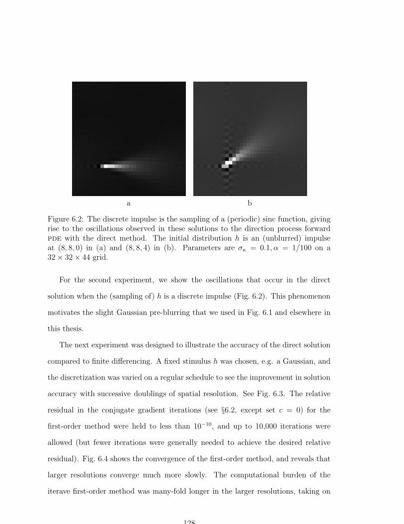
a b

Figure 6.2: The discrete impulse is the sampling of a (periodic) sinc function, givingrise to the oscillations observed in these solutions to the direction process forwardpde with the direct method. The initial distribution h is an (unblurred) impulseat (8, 8, 0) in (a) and (8, 8, 4) in (b). Parameters are σκ = 0.1, α = 1/100 on a32× 32× 44 grid.

For the second experiment, we show the oscillations that occur in the direct

solution when the (sampling of) h is a discrete impulse (Fig. 6.2). This phenomenon

motivates the slight Gaussian pre-blurring that we used in Fig. 6.1 and elsewhere in

this thesis.

The next experiment was designed to illustrate the accuracy of the direct solution

compared to finite differencing. A fixed stimulus h was chosen, e.g. a Gaussian, and

the discretization was varied on a regular schedule to see the improvement in solution

accuracy with successive doublings of spatial resolution. See Fig. 6.3. The relative

residual in the conjugate gradient iterations (see §6.2, except set c = 0) for the

first-order method were held to less than 10−10, and up to 10,000 iterations were

allowed (but fewer iterations were generally needed to achieve the desired relative

residual). Fig. 6.4 shows the convergence of the first-order method, and reveals that

larger resolutions converge much more slowly. The computational burden of the

iterave first-order method was many-fold longer in the larger resolutions, taking on

128

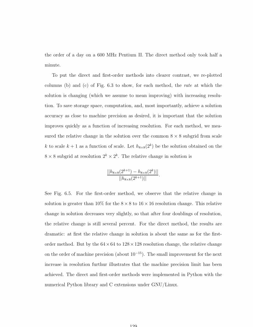
the order of a day on a 600 MHz Pentium II. The direct method only took half a

minute.

To put the direct and first-order methods into clearer contrast, we re-plotted

columns (b) and (c) of Fig. 6.3 to show, for each method, the rate at which the

solution is changing (which we assume to mean improving) with increasing resolu-

tion. To save storage space, computation, and, most importantly, achieve a solution

accuracy as close to machine precision as desired, it is important that the solution

improves quickly as a function of increasing resolution. For each method, we mea-

sured the relative change in the solution over the common 8× 8 subgrid from scale

k to scale k + 1 as a function of scale. Let h8×8(2k) be the solution obtained on the

8× 8 subgrid at resolution 2k × 2k. The relative change in solution is

||h8×8(2k+1)− h8×8(2

k)||||h8×8(2k+1)|| .

See Fig. 6.5. For the first-order method, we observe that the relative change in

solution is greater than 10% for the 8× 8 to 16× 16 resolution change. This relative

change in solution decreases very slightly, so that after four doublings of resolution,

the relative change is still several percent. For the direct method, the results are

dramatic: at first the relative change in solution is about the same as for the first-

order method. But by the 64×64 to 128×128 resolution change, the relative change

on the order of machine precision (about 10−15). The small improvement for the next

increase in resolution furthur illustrates that the machine precision limit has been

achieved. The direct and first-order methods were implemented in Python with the

numerical Python library and C extensions under GNU/Linux.

129

a b c d

Figure 6.3: Comparison of solution improvement with increased spatial resolution.The direction process forward pde was solved on [0, 1]2× [0, 2π] with periodic bound-ary conditions for input b a Gaussian centered at (1/2,1/2,3/8) with standard de-viation 1/16 in all three dimensions. Parameter values are σκ = α = 1. In column(a) are shown the integrals over θ for the direct method solution, for discretizationn × n × 16, where n = 8, 16, 32, 64, 128 (top to bottom) and ∆x = ∆y = 1/n. Tofacilitate comparison, column (b) shows the solution in column (a) subsampled to an8× 8 grid. Observe the slight change from the 8× 8 to the 16× 16 resolution, withno visible improvement thereafter (also see Fig. 6.5). In columns (d) and (c) are thecorresponding results for the first-order method.

130

1e-10

1e-08

1e-06

0.0001

0.01

1

100

0 500 1000 1500 2000 2500 3000 3500

Rel

ativ

e re

sidu

al

Iteration

16 x 16 x 1664 x 64 x 16

256 x 256 x 16

Figure 6.4: Decrease in relative residual (for the first-order method of computing thedirection process forward pde solution) with iterations of conjugate gradient method.Each plot is for the same Gaussian input (see text) sampled at the resolutions shown.

6.1.2 Curvature Process

To compute the action f of the Green’s operator G for the curvature process on

a vector h, we recall the curvature process generator (2.7) to set up the curvature

process forward pde

αf − σ2

2

∂2f

∂κ2+ cos θ

∂f

∂x+ sin θ

∂f

∂y+ κ

∂f

∂θ= h, (6.5)

where σ = σκ > 0. The action of the Green’s operator G is then defined as our

numerical solution to (6.5). To balance performance and simplicity, we use a com-

bination of finite differencing and basis projection. To keep the desired rotational

isotropy and solution focus, we project f with respect to only the x-, y-, and θ-

131

1e-16

1e-14

1e-12

1e-10

1e-08

1e-06

0.0001

0.01

1

8-16 16-32 32-64 64-128 128-256

Rel

ativ

e ch

ange

in s

olut

ion

Resolution change

directfirst-order

Figure 6.5: Rate of improvement in solution with increase in resolution. See text.

dimensions on the same complex exponential basis that we used for the direction

process to obtain fjkl(κ) := 〈f(·, ·, ·, κ), φjkl〉 2× for frequencies j, k, and l. The

κ-dimension is discretized into M uniform samples using finite differencing, as fol-

lows. We first write fjkl;m′ = fjkl(m′∆κ), where κ = m′∆κ for integer m′ and

stepsize ∆κ > 0. The input h is discretized similarly. Then we approximate ∂2f∂κ2 with

(gm′−1 − 2gm′ + gm′+1)/(∆κ)2, for gm′ := f(x, y, θ,m′∆κ).

Taking the (x, y, θ)-projection of (6.5) onto the complex exponential basis, we can

reuse the direction process results, noting that 〈 ∂f∂θ, φjkl〉

2× =lfjkl;m′. We assume

the same bandlimitedness (with respect to (x, y, θ)) of h as in the direction process,

and so are led to solve for the lowest J,K, L frequencies in (x, y, θ) of f in terms of

those of h. Combined with the finite difference approximation in κ, we now need to

132

solve

(α +

σ2

(∆κ)2+

lm′∆κ

)fj,k,l;m′ − σ2

2(∆κ)2

(fj,k,l;m′−1 + fj,k,l;m′+1

)

+π

( j

xmax

+k

ymax

)fj,k,l−1;m′ + π

( j

xmax

− k

ymax

)fj,k,l+1;m′ = hj,k,l;m′. (6.6)

The same periodic boundary condition in l is used as in the direction process case.

We use zero boundary conditions in m′ to put an upper bound on curvature.

Observe that for each j and k, equation (6.6) is an (L ·M)× (L ·M) sparse linear

system in l and m′. Although the computationally advantageous tridiagonality of

the directional process case has been lost, we note that we are often interested in

small L and M (the numbers of discrete directions and curvatures, respectively).

The overall complexity of this system is O((JKLM) log(JKLM)) +O(JK(LM)3),

using LU decomposition to solve the linear system.

6.2 Applying the Biased Green’s Operator

In this section we present a method for computing the action f of the biased Green’s

operator Gc on a vector h. Equivalently, we must solve the linear system

−(Q + C)f = h (6.7)

where Q = αI−L and C is a (possibly non-constant) diagonal operator with c = (ci)

along the diagonal. See §3.3 for how this equation arises in the Feynman-Kac formula.

Because of Khas’sminskii’s condition (Proposition 3), we know that there is a unique

solution to this equation as long as c is sufficiently small.

133

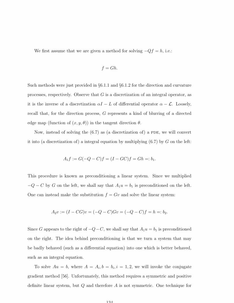
We first assume that we are given a method for solving −Qf = h, i.e.:

f = Gh.

Such methods were just provided in §6.1.1 and §6.1.2 for the direction and curvature

processes, respectively. Observe that G is a discretization of an integral operator, as

it is the inverse of a discretization αI − L of differential operator α − L. Loosely,

recall that, for the direction process, G represents a kind of blurring of a directed

edge map (function of (x, y, θ)) in the tangent direction θ.

Now, instead of solving the (6.7) as (a discretization of) a pde, we will convert

it into (a discretization of) a integral equation by multiplying (6.7) by G on the left:

A1f := G(−Q− C)f = (I −GC)f = Gh =: b1.

This procedure is known as preconditioning a linear system. Since we multiplied

−Q − C by G on the left, we shall say that A1u = b1 is preconditioned on the left.

One can instead make the substitution f = Gv and solve the linear system:

A2v := (I − CG)v = (−Q− C)Gv = (−Q− C)f = h =: b2.

Since G appears to the right of −Q−C, we shall say that A1u = b1 is preconditioned

on the right. The idea behind preconditioning is that we turn a system that may

be badly behaved (such as a differential equation) into one which is better behaved,

such as an integral equation.

To solve Au = b, where A = Ai, b = bi, i = 1, 2, we will invoke the conjugate

gradient method [56]. Unfortunately, this method requires a symmetric and positive

definite linear system, but Q and therefore A is not symmetric. One technique for

134

circumventing the asymmetry of A is to multiply (6.7) on the left by its transpose

A∗, forming the normal equations

A∗Au = A∗b, (6.8)

where A∗A is symmetric because (A∗A)∗ = A∗(A∗)∗ = A∗A and positive definite

because x∗A∗Ax = (Ax)∗(Ax) = ||Ax||2 > 0 for nonsingular A unless x = 0. Now,

we can apply the (iterative) conjugate gradient method directly to (6.8) in order to

solve for u in the sense that the relative residual ||A∗Au − A∗b||/||A∗b|| is reduced

to less than some tolerance level. We can then apply the above definitions to get f

itself.

6.3 Solving for the Biased CIRF Approximation

of the Posterior

In §5.7 we derived coupled nonlinear systems for filtering. Because of the presence

of blur in a number of applications, we elected to solve the nonlinear system in

equations (5.32) and (5.33). Left multiplying these by Q−1 and Q∗−1 respectively,

we get the following system:

f − εGCf + ν ′ = 0 (6.9)

b− εG∗Cb + µ′ = 0, (6.10)

where C := diag(a + 2NA(f b)), ν ′ = Gν, and µ′ = G∗µ. To solve this nonlinear

system, we adopted a continuation strategy in ε. Specifically, we began with ε small,

solved the system, and then used that solution to get an initial condition for the

135

system with ε slightly larger. We proceeded in this fashion until we reached the

value of ε required. To solve this system for any such fixed ε, we used Newton’s

method [56], where often only a few iterations are required because of the Newton

method’s powerful local convergence properties. To bootstrap this continuation pro-

cess with a starting initial condition (corresponding to the smallest value of ε), we

set C = diag(a) (i.e., neglecting the nonlinearity) and then solved the resulting de-

coupled equations, which evidently are the biased cirf Green’s operator equations

that we saw in the previous section. We now apply our filters to images.

136

Chapter 7

Results

In this chapter we illustrate the performance of cirf filters. We begin by applying

direction process-based Volterra filters to some synthetic images and later to a few

natural images. The Volterra filter is also briefly compared to the biased cirf ap-

proximation filter, where the latter shows more powerful noise cleaning action. We

conclude with some examples of the curvature process-based cirf filter.

7.1 Contour Filtering in 2 × with Direction

The first test of the cirf framework was with the mmse Volterra filters using the

direction process in 2 × . With the direct method for computing the action of

G and G∗ from the last chapter, applying these filters requires substitution into

the Volterra formulas in Result 1. We selected parameters as follows. Because the

density parameter η is an overall multiplicative constant, it amounts to a threshold

setting. We developed a user interface to select the parameters ε, ζ, the threshold,

and the order of the filter. By inspection of the Volterra filtering formulas, one can

do most of the computation before parameter selection. Then, for each parameter

setting, only a few fields need to be weighted and added; this means that parameters

137

can be chosen rapidly; typically, selecting parameters took less than a minute. In

most examples we let ζ be small (usually 0) and let ε be about 10, although the exact

setting of ε did not appear to have a great effect. In the end the user interface was

most useful for setting the threshold and comparing the different orders of filter.

Because of the computational efficiency of the Volterra filters, we were able to

test them on a number of examples. To assess the robustness of the Volterra filter in

the presence of noise, we evaluated responses to images of a horizontal straight line

corrupted by additive Gaussian noise of variance σ2N . We characterized the degree

of noisiness using the peak signal-to-noise ratio, which, for an image I taking values

in the range Imin to Imax, is

Peak snr = 20 log10

Imax − Imin

σN,

expressed in decibels. To map from the planar image to a field on discrete 2× , we

simply copied the image to each direction, so that our measurements m = m(x, y, θ)

were constant in θ. We were able to select this mapping because the images were

purely contours embedded in noise. More generally an oriented local edge or line

operator would be applied, as we shall see when we consider natural images.

To avoid the aliasing effect illustrated in Fig. 6.2, for all experiments in this

chapter we convolved the input with a Gaussian having a standard deviation of 1

pixel in all dimensions before applying a cirf filter. The results of applying the

linear, quadratic, and cubic Volterra filters to the noisy line image are shown in Figs.

7.1 and 7.2, where the display is produced by taking the maximum response over

all directions θ for each position (x, y). Observe that while the filter responses are

strongest along the line, there is some response elsewhere, especially for the linear

filters. This extra response can be thought of as weaker contour hypotheses, and

138

conveys how a field model can parsimoniously express the infinite space of contour

explanations. We also observe that as the order of the filter is increased to quadratic

and then cubic, the response becomes increasingly focused on the desired line. To

quantify these results, we placed the responses as vectors in very high-dimensional

spaces. For these 64× 64× 64 fields, the dimension of this space is 262,144. Then,

each response was then centered by subtracting its average value from itself. For each

kind of filter order (linear, quadratic, and cubic), we measured the angle between

the (high-dimensional) vector u1 representing the noiseless (centered) response and

the vector u2 representing the (centered) response under a particular level of noise.

The angle (in degrees) between centered responses u1 and u2 is defined as:

180

πcos−1 〈u1, u2〉

||u1|| ||u2||,

where 〈u1, u2〉 is the Euclidean inner product between u1 and u2, and ||u|| =√〈u, u〉.

Observe the quantitative improvement of the quadratic and cubic nonlinear filters

compared to the linear result (Fig. 7.3); this nonlinear advantage appears even greater

as σκ is made smaller, i.e., when the contours are assumed to be straighter.

To study the effect that the parameters of the direction process have on our fil-

tering results, we created an image containing curves of different curvatures and lines

with gaps, and then applied the direction process-based mmse cirf cubic Volterra

filter at a number of parameter settings (Fig. 7.4). The number of directions used in

each test was 16, 16, 32, and 64, for σκ settings of 1, 0.33, 0.2, and 0.1, respectively;

using more directions has a negligible visible effect. The image at the top was input

to the filter by copying the image over all directions θ (black is 0, and white is 1);

no noise was added, although discretization artifacts are evident in the semi-circular

contour regions. The brightness of the filter outputs (bottom four rows) was obtained

139

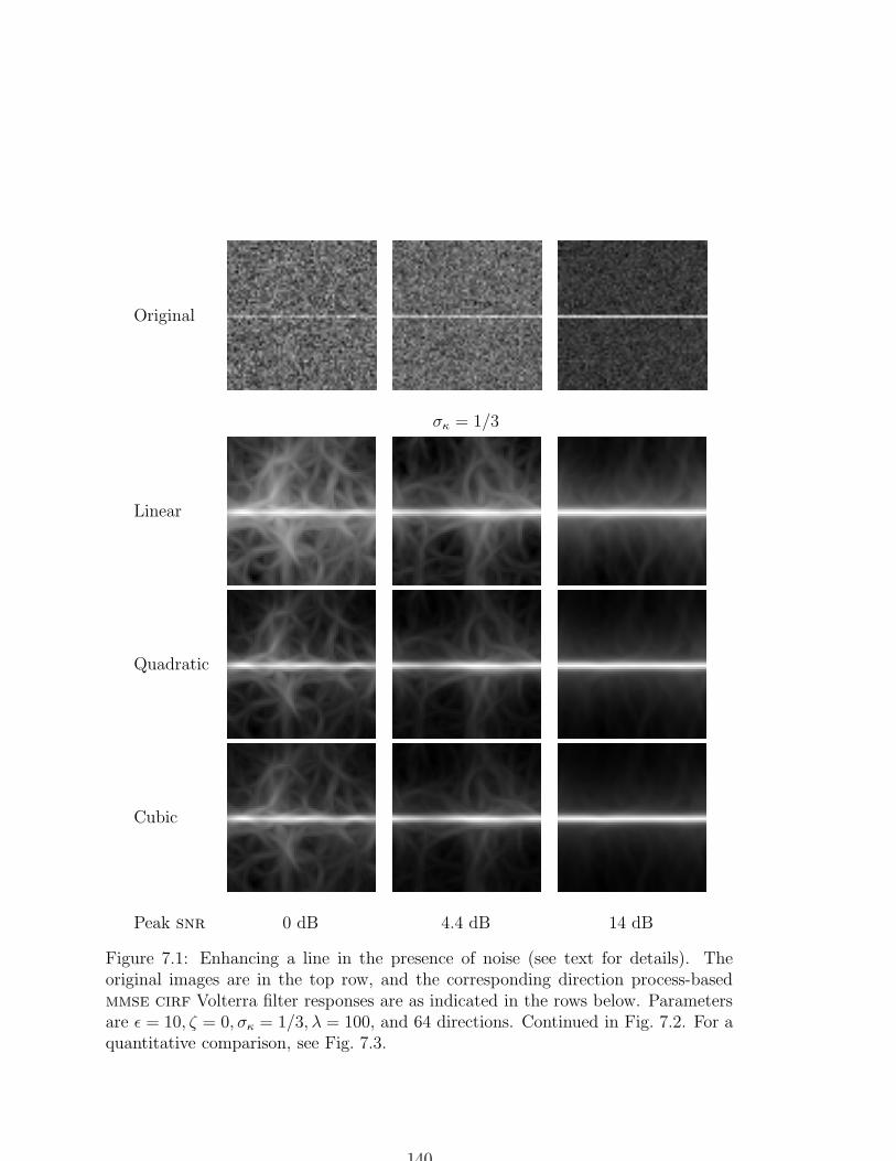
Original

σκ = 1/3

Linear

Quadratic

Cubic

Peak snr 0 dB 4.4 dB 14 dB

Figure 7.1: Enhancing a line in the presence of noise (see text for details). Theoriginal images are in the top row, and the corresponding direction process-basedmmse cirf Volterra filter responses are as indicated in the rows below. Parametersare ε = 10, ζ = 0, σκ = 1/3, λ = 100, and 64 directions. Continued in Fig. 7.2. For aquantitative comparison, see Fig. 7.3.

140

σκ = 1/10

Linear

Quadratic

Cubic

Peak snr 0 dB 4.4 dB 14 dB

Figure 7.2: Enhancing a line in the presence of noise (continued from Fig. 7.1).Parameters are ε = 10, ζ = 0, σκ = 1/10, λ = 100, and 64 directions. Observethe much-reduced response away from the curve compared to the case σκ = 1/3 inFig. 7.1, especially in the quadratic and cubic Volterra responses. For a quantitativecomparison, see Fig. 7.3.

from the maximum response over all directions θ at each position (x, y). Values of

σκ that we have often used in experimenting with the Volterra filters correspond to

the bottom three rows. For λ = 100 (a typical value in our work), we observe that

the gaps are partially filled at σκ = 0.33, and are more strongly completed as σκ is

decreased to 0.1. However, the small half-circle in the center is attenuated at small

σκ, as large curvatures in the direction process become more improbable. Because

the filter output is not sensitive to variations in λ when λ is large (around 100, say),

we used a logarithmic scale in λ. For λ = 10, slightly greater attenuation in the gaps

141

Volterra Filter Performance (σκ = 1/3)

0

5

10

15

20

25

30

35

40

0.0 1.9 4.4 8.0 14.0 ∞

Ang

le [d

egre

es]

Peak SNR [dB]

linearquadratic

cubic

Volterra Filter Performance (σκ = 1/10)

0

5

10

15

20

25

30

35

40

45

0.0 1.9 4.4 8.0 14.0 ∞

Ang

le [d

egre

es]

Peak SNR [dB]

linearquadratic

cubic

Figure 7.3: Noise performance of direction process-based mmse cirf Volterra filters.Plotted is the angle between the centered filter responses to the noisy and noise-freeimages shown in Fig. 7.1 (top plot above) and Fig. 7.2 (bottom plot above); see textfor details.

142

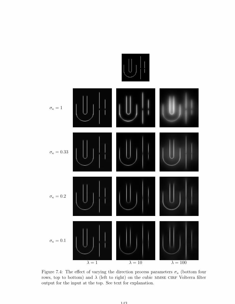
σκ = 1

σκ = 0.33

σκ = 0.2

σκ = 0.1

λ = 1 λ = 10 λ = 100

Figure 7.4: The effect of varying the direction process parameters σκ (bottom fourrows, top to bottom) and λ (left to right) on the cubic mmse cirf Volterra filteroutput for the input at the top. See text for explanation.

143

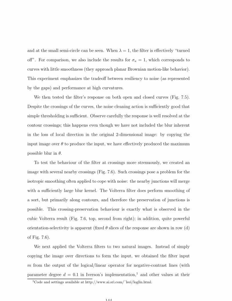
and at the small semi-circle can be seen. When λ = 1, the filter is effectively “turned

off”. For comparison, we also include the results for σκ = 1, which corresponds to

curves with little smoothness (they approach planar Brownian motion-like behavior).

This experiment emphasizes the tradeoff between resiliency to noise (as represented

by the gaps) and performance at high curvatures.

We then tested the filter’s response on both open and closed curves (Fig. 7.5).

Despite the crossings of the curves, the noise cleaning action is sufficiently good that

simple thresholding is sufficient. Observe carefully the response is well resolved at the

contour crossings; this happens even though we have not included the blur inherent

in the loss of local direction in the original 2-dimensional image: by copying the

input image over θ to produce the input, we have effectively produced the maximum

possible blur in θ.

To test the behaviour of the filter at crossings more strenuously, we created an

image with several nearby crossings (Fig. 7.6). Such crossings pose a problem for the

isotropic smoothing often applied to cope with noise: the nearby junctions will merge

with a sufficiently large blur kernel. The Volterra filter does perform smoothing of

a sort, but primarily along contours, and therefore the preservation of junctions is

possible. This crossing-preservation behaviour is exactly what is observed in the

cubic Volterra result (Fig. 7.6, top, second from right); in addition, quite powerful

orientation-selectivity is apparent (fixed θ slices of the response are shown in row (d)

of Fig. 7.6).

We next applied the Volterra filters to two natural images. Instead of simply

copying the image over directions to form the input, we obtained the filter input

m from the output of the logical/linear operator for negative-contrast lines (with

parameter degree d = 0.1 in Iverson’s implementation,1 and other values at their

1Code and settings available at http://www.ai.sri.com/˜leei/loglin.html.

144

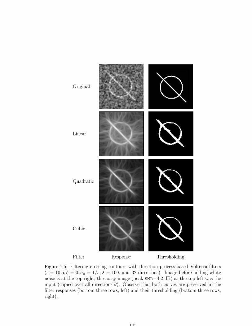
Original

Linear

Quadratic

Cubic

Filter Response Thresholding

Figure 7.5: Filtering crossing contours with direction process-based Volterra filters(ε = 10.5, ζ = 0, σκ = 1/5, λ = 100, and 32 directions). Image before adding whitenoise is at the top right; the noisy image (peak snr=4.2 dB) at the top left was theinput (copied over all directions θ). Observe that both curves are preserved in thefilter responses (bottom three rows, left) and their thresholding (bottom three rows,right).

145

a

b

c

d

e

θ : 0 45 90 135

Figure 7.6: Crossing lines are teased apart with the cubic Volterra filter. From left toright in row (a): original image, image corrupted with additive white Gaussian noise(peak snr=8 dB), cubic Volterra filter response (ε = 10.5, ζ = 0, σκ = 1/10, λ =100, and 64 directions), and thresholded response. Noisy image was copied over alldirections to form filter input (row (b); for comparison we include the correspondingnoise-free “stack” of direction-specific images in row (c)), then filtered with the high-noise mmse cirf cubic Volterra filter (row (d)), and thresholded (row (e)). Observehow the initially strong responses at the inappropriate directions are chiseled awayby the action of the filter, despite the presence of noise.

146

Image Local Responses Thresholding

Figure 7.7: Fluoroscopic image of guide wire (left), logical/linear negative-contrastline responses (center) and their thresholding (right). See Fig. 7.8 for Volterra filter-ing results.

default). The first example is of a guide wire imaged fluoroscopically during surgery

(Fig. 7.7). Finding the wire in noise is particularly important, because surgery can

take hours, all the while exposing the patient to radiation. Reducing such radiation

exposures unfortunately also increases the noise level and makes local filtering (e.g.,

edge and line operators) perform more poorly. With the mmse cirf Volterra filters,

we can readily enhance the guide wire contour (Fig. 7.8).

Another example is the ship’s wake shown in Fig. 7.9 (top left). For this demon-

stration, we work with the magnified section shown in Fig. 7.9 (top right), and

then obtain logical/linear negative-contrast line responses (with degree 0.1) and their

thresholding (second row). Responses to high-noise Volterra filters (Result 1) for the

direction process-based CIRF (ε = 10.5, ζ = 0, σκ = 1/15, λ = 100, and 96 directions)

is shown in the bottom three rows of Fig. 7.9. To produce these two dimensional

images from the actual discrete (x, y, θ)-space responses, the maximum over θ was

147

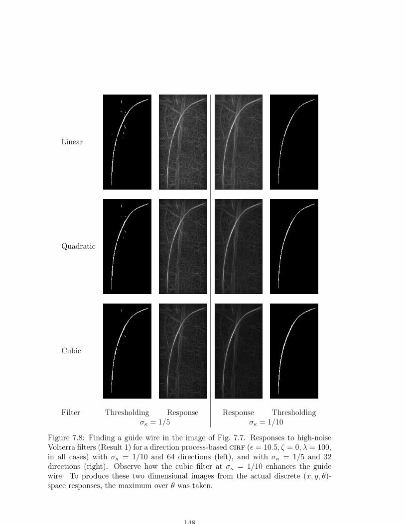
Linear

Quadratic

Cubic

Filter Thresholding Response Response Thresholdingσκ = 1/5 σκ = 1/10

Figure 7.8: Finding a guide wire in the image of Fig. 7.7. Responses to high-noiseVolterra filters (Result 1) for a direction process-based cirf (ε = 10.5, ζ = 0, λ = 100,in all cases) with σκ = 1/10 and 64 directions (left), and with σκ = 1/5 and 32directions (right). Observe how the cubic filter at σκ = 1/10 enhances the guidewire. To produce these two dimensional images from the actual discrete (x, y, θ)-space responses, the maximum over θ was taken.

148

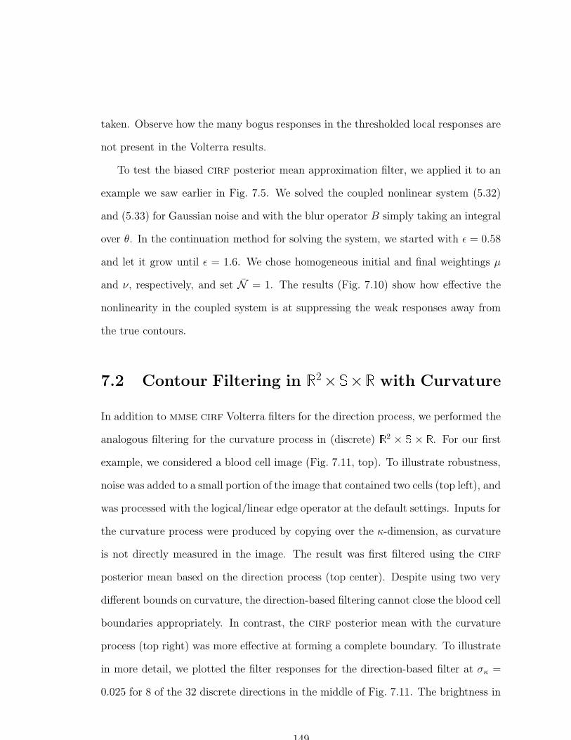
taken. Observe how the many bogus responses in the thresholded local responses are

not present in the Volterra results.

To test the biased cirf posterior mean approximation filter, we applied it to an

example we saw earlier in Fig. 7.5. We solved the coupled nonlinear system (5.32)

and (5.33) for Gaussian noise and with the blur operator B simply taking an integral

over θ. In the continuation method for solving the system, we started with ε = 0.58

and let it grow until ε = 1.6. We chose homogeneous initial and final weightings µ

and ν, respectively, and set N = 1. The results (Fig. 7.10) show how effective the

nonlinearity in the coupled system is at suppressing the weak responses away from

the true contours.

7.2 Contour Filtering in 2× ×

with Curvature

In addition to mmse cirf Volterra filters for the direction process, we performed the

analogous filtering for the curvature process in (discrete) 2 × ×

. For our first

example, we considered a blood cell image (Fig. 7.11, top). To illustrate robustness,

noise was added to a small portion of the image that contained two cells (top left), and

was processed with the logical/linear edge operator at the default settings. Inputs for

the curvature process were produced by copying over the κ-dimension, as curvature

is not directly measured in the image. The result was first filtered using the cirf

posterior mean based on the direction process (top center). Despite using two very

different bounds on curvature, the direction-based filtering cannot close the blood cell

boundaries appropriately. In contrast, the cirf posterior mean with the curvature

process (top right) was more effective at forming a complete boundary. To illustrate

in more detail, we plotted the filter responses for the direction-based filter at σκ =

0.025 for 8 of the 32 discrete directions in the middle of Fig. 7.11. The brightness in

149

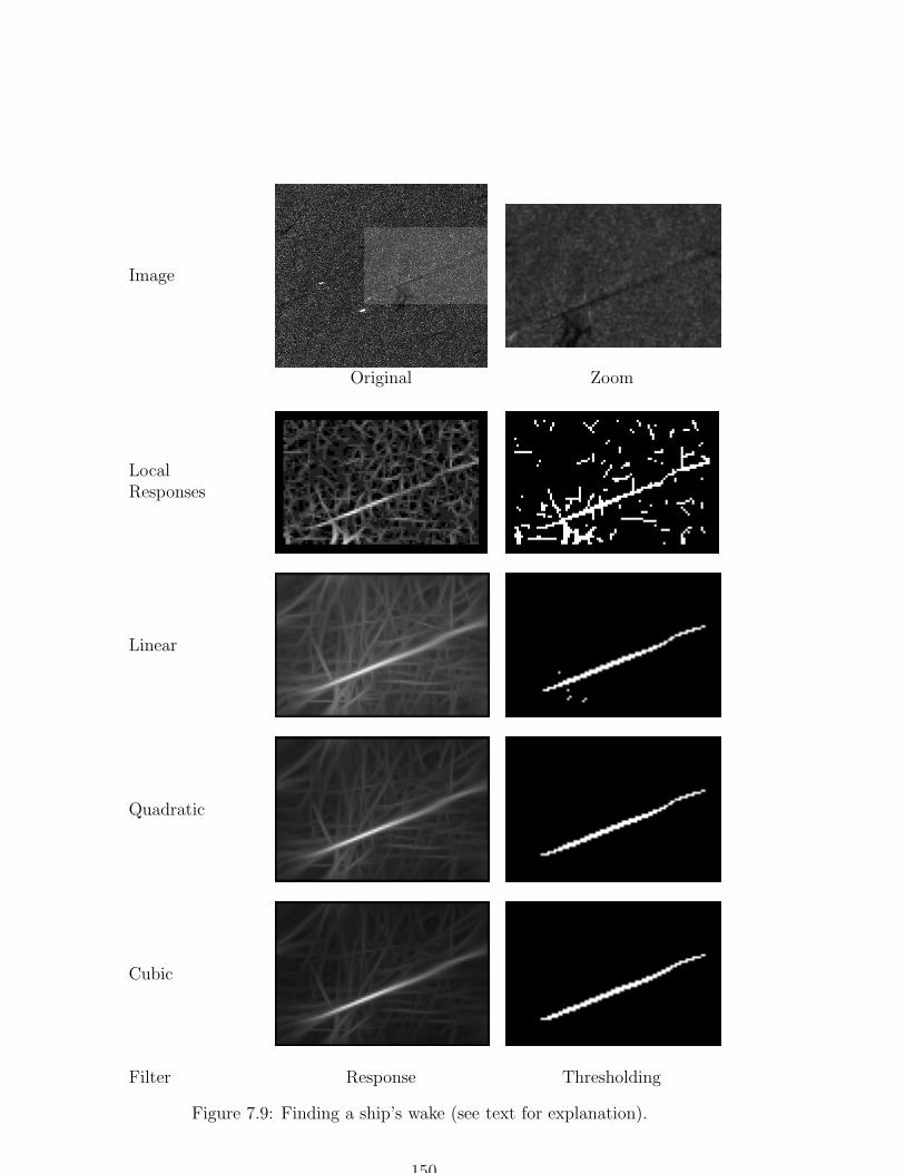
Image

Original Zoom

LocalResponses

Linear

Quadratic

Cubic

Filter Response Thresholding

Figure 7.9: Finding a ship’s wake (see text for explanation).

150

a b

c d e

0 45 90 135

Figure 7.10: Filtering with the biased cirf posterior mean approximation. (a) Origi-nal image, (b) noisy version copied over θ to form input m to filter, (c) cubic Volterraresult (ε = 10.5, ζ = 0, σκ = 1/3, with 16 directions), (d) biased cirf result at startof continuation method (ε = 0.58), (e) final biased cirf result at end of continuationmethod (ε = 1.6). Bottom three rows are (from top to bottom): response over θfor cubic Volterra filter; for biased cirf approximation at start of continuation; andfor biased cirf approximation at the end of the continuation method. Observe thestriking degree of orientation selectivity in the biased cirf approximation end result.

151

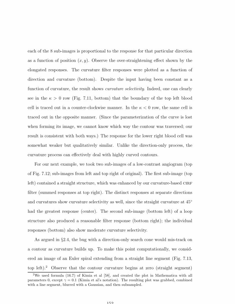
each of the 8 sub-images is proportional to the response for that particular direction

as a function of position (x, y). Observe the over-straightening effect shown by the

elongated responses. The curvature filter responses were plotted as a function of

direction and curvature (bottom). Despite the input having been constant as a

function of curvature, the result shows curvature selectivity. Indeed, one can clearly

see in the κ > 0 row (Fig. 7.11, bottom) that the boundary of the top left blood

cell is traced out in a counter-clockwise manner. In the κ < 0 row, the same cell is

traced out in the opposite manner. (Since the parameterization of the curve is lost

when forming its image, we cannot know which way the contour was traversed; our

result is consistent with both ways.) The response for the lower right blood cell was

somewhat weaker but qualitatively similar. Unlike the direction-only process, the

curvature process can effectively deal with highly curved contours.

For our next example, we took two sub-images of a low-contrast angiogram (top

of Fig. 7.12; sub-images from left and top right of original). The first sub-image (top

left) contained a straight structure, which was enhanced by our curvature-based cirf

filter (summed responses at top right). The distinct responses at separate directions

and curvatures show curvature selectivity as well, since the straight curvature at 45

had the greatest response (center). The second sub-image (bottom left) of a loop

structure also produced a reasonable filter response (bottom right); the individual

responses (bottom) also show moderate curvature selectivity.

As argued in §2.4, the bug with a direction-only search cone would mis-track on

a contour as curvature builds up. To make this point computationally, we consid-

ered an image of an Euler spiral extending from a straight line segment (Fig. 7.13,

top left).2 Observe that the contour curvature begins at zero (straight segment)

2We used formula (16.7) of Kimia et al [58], and created the plot in Mathematica with allparameters 0, except γ = 0.1 (Kimia et al’s notation). The resulting plot was grabbed, combinedwith a line segment, blurred with a Gaussian, and then subsampled.

152

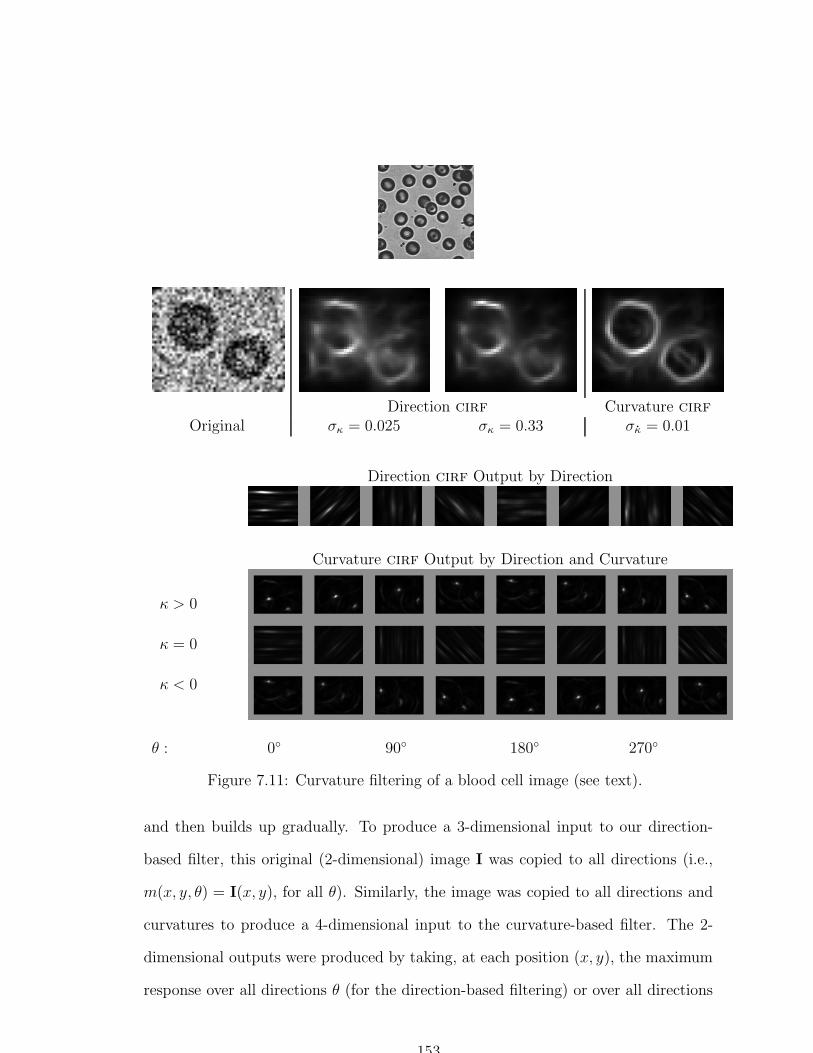
Direction cirf Curvature cirf

Original σκ = 0.025 σκ = 0.33 σκ = 0.01

Direction cirf Output by Direction

κ > 0

κ = 0

κ < 0

Curvature cirf Output by Direction and Curvature

θ : 0 90 180 270

Figure 7.11: Curvature filtering of a blood cell image (see text).

and then builds up gradually. To produce a 3-dimensional input to our direction-

based filter, this original (2-dimensional) image I was copied to all directions (i.e.,

m(x, y, θ) = I(x, y), for all θ). Similarly, the image was copied to all directions and

curvatures to produce a 4-dimensional input to the curvature-based filter. The 2-

dimensional outputs were produced by taking, at each position (x, y), the maximum

response over all directions θ (for the direction-based filtering) or over all directions

153

κ > 0

κ = 0

κ < 0

Curvature cirf Output by Direction and Curvature

θ : 0 45 90 135

κ > 0

κ = 0

κ < 0

Curvature cirf Output by Direction and Curvature

θ : 0 45 90 135

Figure 7.12: Curvature filtering for an angiogram (see text).

154

θ and curvatures κ (for the curvature-based filtering). The direction-based cirf pos-

terior mean (with parameters σκ = 0.025, λ = 10, and 64 directions) was computed

(left, rows (a) and (b)), showing an undesirable reduction in response as curvature

built up. The curvature-based cirf posterior mean (left, rows (c) and (d), with pa-

rameters σκ = 0.05, λ = 10, 64 directions, and 7 curvatures (0,±0.05,±0.1,±0.15))

shows strong response even at the higher curvature portions of the contour. To test

robustness, 0-mean Gaussian noise of standard deviation 0.5 was added (top right)

to the image (0 to 1 was the signal range before adding noise). The results (right,

rows (a)-(d)) show that the curvature-based filter performs better in high curvature

regions despite noise.

155

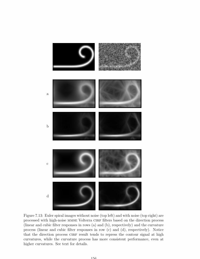
a

b

c

d

Figure 7.13: Euler spiral images without noise (top left) and with noise (top right) areprocessed with high-noise mmse Volterra cirf filters based on the direction process(linear and cubic filter responses in rows (a) and (b), respectively) and the curvatureprocess (linear and cubic filter responses in row (c) and (d), respectively). Noticethat the direction process cirf result tends to repress the contour signal at highcurvatures, while the curvature process has more consistent performance, even athigher curvatures. See text for details.

156

Chapter 8

Conclusion

In this thesis we have introduced a field structure intermediate between contours

and the images that suggest them. This curve indicator random field was studied for

Markov process contour models, leading to a practical description of its joint statis-

tical structure via a moment generating functional. By relating contours to images,

the model provides a way to verify whether it is in agreement with natural image

structure; in this way a role for curvature was found, motivating our introduction of

a Markov process in contour curvature. We believe that the cirf is so basic that

future work on visual contours will have difficulty avoiding it.

Enhancing contour structure in noisy images was characterized as mmse esti-

mation of an underlying cirf, and a variety of nonlinear filters were provided for

computing this posterior mean estimate. The Volterra filters emphasized high-noise

situations, and results on synthetic and real images verified this. The more power-

ful reaction-diffusion-convection equation was provided for dealing with blur more

accurately. We note that this pde was not derived as an (explicit) Euler-Lagrange

equation; instead, it arose indirectly via the moment generating functional of the

biased cirf.

157

Besides enabling explicit calculations, the cirf provides a handle on a rather

unpleasant aspect of contours: their global structure. In particular, the square of

the cirf measures contour intersections. We note that this was not suggested by

studying the cirf prior itself; instead it arose as a quadratic term in the likelihood.

In hindsight, however, it can just as easily be incorporated into the cirf prior to

discourage intersections (see §5.2.3). No current scheme for contour inference has a

place for these interactions, although it is not surprising that dealing with multiple

contours must eventually confront the intersection problem.

8.1 Future Directions

The work in this thesis can be both focused and broadened in a number of ways. On

the practical side, the estimation of the parameters used in the cirf filters would

be convenient for further automating their use. More interesting is the issue of

learning the Markov process contour model. At its simplest, this could be viewed as

a model selection problem, perhaps for choosing between the direction and curvature

processes. More generally, one might like to learn the Markov process generator itself,

using empirical edge correlations of training curve images, for example.

Even more important for applications may be the estimation of good observation

models. We have outlined how the Geman and Jedynak scheme [35] of on-edge

and off-edge distributions can be incorporated. Clearly more realism is desirable; of

highest priority is probably blur scale; currently, our scheme is implemented at one

scale with the direction and curvature processes.

Another immediate issue is occlusion, which is a fundamental example of contour

intersection. Can this be formalized with a quadratic log-likelihood observation

model? Possibly, because occlusion suggests a competitive interaction, where the

158

presence of a contour would discourage other contours on one side (the occluding

side). Another aspect of interaction is texture flow [49], where approximately parallel

nearby contours merge into a flow field of local orientations.

Interaction is also relevant for branching structures, such as vascular structures

in the human body. One can formalize this using branching Markov process (super-

processes). This would be particularly important for medical imaging.

Both closure and symmetry can be thought of as interactions of another form,

by representing the contour with its skeleton or symmetry set. Such a model would

allow us to characterize regional properties of the shape, such as symmetry of two

portions of boundary. Even though symmetry is not a local property of the boundary,

it is a local property of the skeleton. We can construct a branching Markov process

for such a medial axis description that can specify symmetry information through

the radius function and axis location (and derivatives). Two local constraints that

must be maintained in the process are: (1) the radius of curvature of the skeleton is

bounded below by the radius and (2) the rate of change of radius is less than unity

(local growth). Closure (of the boundary induced by the skeleton) is maintained by

construction. The key complication introduced here is the need for a cirf repre-

sentation for the boundary and another for the skeleton. For consistency, these two

cirfs will have to be coupled so that they correspond to the same shapes.

There are a number of interesting technical issues related to the cirf. For ex-

ample, what is the role of the (approximate) self-avoidingness of the Markov process

models, and how does this relate to the intersection terms in the likelihood? While

functions of Markov processes are generally not themselves Markovian, is there even

an approximate sense in which the cirf, as a random field, is Markovian? How is

this related to contour self-avoidingness? On a simpler note, it would be useful to

159

know how to solve for the initial and final weightings on contour endpoints in terms

of given endpoint marginal distributions (Remark 1).

Mathematically, it would also be useful to know some basic properties of the

filtering equations we have provided. Do solutions exist? Are they unique? For the

Volterra filters these questions are trivial, but for the biased cirf approximation

these questions are more subtle.

In a more speculative direction, one may also extend the framework presented

here beyond contours, to submanifolds of dimension greater than one. Inspired

by applications of relaxation labeling [105], surfaces would be the most important

immediate extension; one could define an analogous surface indicator random field

(sirf) to support medical imaging applications, for example. One goal would be to

estimate the sirf that corresponds to the intestinal wall or the surface of a brain

from cat or mri images.

It is the hope of this work that it encourages the field of computer vision to con-

sider taking low-level information, aided by generic geometrical priors, more seriously

as a foundation for general vision systems.

160

Bibliography

[1] P. Alper. A consideration of discrete volterra series. IEEE Transactions on

Automatic Control, 10:322–327, 1965.

[2] H. C. Andrews and B. R. Hunt. Digital Image Restoration. Prentice-Hall,

Englewood Cliffs, NJ, 1977.

[3] J. August and S. W. Zucker. The curve indicator random field: curve orga-

nization via edge correlation. In K. Boyer and S. Sarkar, editors, Perceptual

Organization for Artificial Vision Systems, pages 265–288. Kluwer Academic,

Boston, 2000.

[4] J. August and S. W. Zucker. The moments of the curve indicator random field.

In Proceedings of the 2000 Conference on Information Sciences and Systems,

volume 1, pages WP5–19–WP5–24, Princeton, NJ, March 2000.

[5] J. August and S. W. Zucker. Organizing curve elements with an indicator

random field on the (unit) tangent bundle. In IEEE Workshop on Perceptual

Organization in Computer Vision, Corfu, September, 1999.

[6] P. Belhumeur. A bayesian-approach to binocular stereopsis. IJCV, 19(3):237–

260, August 1996.

161

[7] J. Biemond, R. L. Lagendijk, and R. M. Mersereau. Iterative methods for

image deblurring. Proc. IEEE, 78(5):856–883, 1990.

[8] J. Biemond, J. Rieske, and J. J. Gerbrands. A fast kalman filter for images

degraded by both blur and noise. IEEE Transactions on Acoustics, Speech,

and Signal Processing, 31:1248–1256, 1983.

[9] A. Blake and A. Zisserman. Visual Reconstruction. MIT Press, Cambridge,

MA, 1987.

[10] P. Bondon, P. L. Combettes, and B. Picinbono. Volterra filtering and higher

order whiteness. IEEE Transactions on Signal Processing, 43(9):2209–2212,

1995.

[11] J. Canny. A computational approach to edge detection. IEEE Transactions

on Pattern Analysis and Machine Intelligence, 8:679–698, 1986.

[12] S. Casadei and S. Mitter. Hierarchical image segmentation – Part I: Detection

of regular curves in a regular graph. International Journal of Computer Vision,

27(3):71–100, 1998.

[13] G. Casella and R. L. Berger. Statistical Inference. Duxbury, Belmont, CA,

1990.

[14] D. E. Catlin. Estimation, Control, and the Discrete Kalman Filter. Springer,

New York, 1989.

[15] I. J. Cox, J. M. Rehg, and S. Hingorani. A Bayesian Multiple-Hypothesis

Approach to Edge Grouping and Contour Segmentation. International Journal

of Computer Vision, 11:5–24, 1993.

162

[16] J. G. Daugman. Uncertainty relation for resolution in space, spatial frequency,

and orientation optimized by two-dimensional visual cortical filters. J. Opt.

Soc. Am. A, 2(7):1160–1169, 1985.

[17] A. Desolneux, L. Moisnan, and J.-M. Morel. Meaningful alignments. Interna-

tional Journal of Computer Vision, 40(1):7–23, 2000.

[18] A. Desolneux, L. Moisnan, and J.-M. Morel. Edge detection by helmholtz

principle. Journal of Mathematical Imaging and Vision, 14:271–284, 2001.

[19] A. Dobbins, S. W. Zucker, and M. S. Cynader. Endstopped neurons in the

visual cortex as a substrate for calculating curvature. Nature, 329(6138):438–

441, 1987.

[20] R. O. Duda and P. E. Hart. Pattern Classification and Scene Analysis. Wiley,

New York, 1973.

[21] J. S. Duncan and T. Birkholzer. Reinforcement of linear structure using

parametrized relaxation labeling. IEEE Transactions on Pattern Analysis and

Machine Intelligence, 14(5):502–515, 1992.

[22] E. B. Dynkin. Markov processes as a tool in field theory. Journal of Functional

Analysis, 50:167–187, 1983.

[23] E. B. Dynkin. Gaussian and non-gaussian fields associated with markov pro-

cesses. Journal of Functional Analysis, 55:344–376, 1984.

[24] E. B. Dynkin. Local times and quantum fields. In Seminar on Stochastic

Processes, 1983, pages 69–83, Boston, 1984. Birkh auser.

163

[25] J. Elder and A. Krupnik. Contour grouping with strong prior models. In The

3rd Workshop on Perceptual Organization in Computer Vision, Vancouver,

2001.

[26] J. H. Elder. The Visual Computation of Bounding Contours. PhD thesis,

McGill University, 1995.

[27] R. J. Elliott, L. Aggoun, and J. B. Moore. Hidden Markov Models: Estimation

and Control. Springer, 1994.

[28] L. Euler. Methodus inveniendi lineas curvas maximi minimive proprietate gau-

dentes. Lausanne, 1744.

[29] D. J. Field, A. Hayes, and R. Hess. Contour integration by the human visual

system: Evidence for an a local ‘association field’. Vision Research, 33:173–193,

1993.

[30] P. J. Fitzsimmons and J. Pitman. Kac’s moment formula and the feynman-kac

formula for additive functionals of a markov process. Stochastic Processes and

their Applications, 79:117–134, 1999.

[31] L. Florack. The Syntactical Structure of Scalar Images. PhD thesis, Utrecht

University, 1993.

[32] L. Florack, B. ter Haar Romeny, M. Viergever, and J. Koenderink. The gaus-

sian scale-space paradigm and the multiscale local jet. International Journal

of Computer Vision, 18:61–75, 1996.

[33] L. M. J. Florack, B. M. ter Haar Romeny, J. J. Koenderink, and M. A.

Viergever. Scale and the differential structure of images. Image and Vision

Computing, 10(6):376–388, August 1992.

164

[34] W. S. Geisler, J. S. Perry, B. J. Super, and D. P. Gallogly. Edge co-occurrence

in natural images predicts contour grouping performance. Vision Research,

41:711–724, 2001.

[35] D. Geman and B. Jedynak. An active testing model for tracking roads in satel-

lite images. IEEE Transactions on Pattern Analysis and Machine Intelligence,

18(1):1–14, 1996.

[36] S. Geman and D. Geman. Stochastic relaxation, gibbs distributions, and the

bayesian restoration of images. IEEE Transactions on Pattern Analysis and

Machine Intelligence, 6(6):721–741, 1984.

[37] G. H. Granlund and H. Knutsson. Signal Processing for Computer Vision.

Kluwer Academic, Dordrecht, 1995.

[38] U. Grenander and M. I. Miller. Representations of knowledge in complex-

systems. Journal of the Royal Statistical Society Series B-Methodological,

56(4):549–603, 1994.

[39] G. Guy and G. Medioni. Inferring global perceptual contours from local fea-

tures. International Journal of Computer Vision, 20(1/2):113–133, 1996.

[40] E. R. Hancock and J. Kittler. Edge-labeling using dictionary-based relaxation.

IEEE Transactions on Pattern Analysis and Machine Intelligence, 12(2):165–

181, 1990.

[41] C. W. Helstrom. Probability and Stochastic Processes for Engineers. Macmillan, New

York, 1991.

[42] L. Herault and R. Horaud. Figure-ground discrimination: A combinatorial optimiza-

tion approach. IEEE Transactions on Pattern Analysis and Machine Intelligence,

15(9):899–914, 1993.

165

[43] B. K. P. Horn. The Curve of Least Energy. ACM Transactions on Mathematical

Software, 9:441–460, 1983.

[44] J. Huang and D. Mumford. Statistics of natural images and models. In Pro-

ceedings, Computer Vison and Pattern Recognition, pages 541–547, 1999.

[45] D. H. Hubel and T. N. Wiesel. Functional architecture of macaque monkey

visual cortex. Proc. R. Soc. Lond. B, 198:1–59, 1977.

[46] M. H. Hueckel. An operator which locates edges in digitized pictures. Journal

of the Association for Computing Machinery, 18(1):113–125, 1971.

[47] R. Hummel and S. W. Zucker. On the foundations of relaxation labeling

processes. IEEE Transactions on Pattern Analysis and Machine Intelligence,

6:267–287, 1983.

[48] M. Isard and A. Blake. Condensation: conditional density propagation for

visual tracking. International Journal of Computer Vision, 29(1):5–28, 1998.

[49] L. A. Iverson. Toward Discrete Geometric Models for Early Vision. PhD thesis,

McGill University, Montreal, 1994.

[50] L. A. Iverson and S. W. Zucker. Logical/linear operators for image curves.

IEEE Transactions on Pattern Analysis and Machine Intelligence, 17(10):982–

996, 1995.

[51] S. N. Kalitzin, B. M. ter Haar Romeny, and M. A. Viergever. Invertible ori-

entation bundles on 2d scalar images. In Proc. Scale-Space ’97, LICS, pages

77–88. Springer, 1997.

[52] G. Kanizsa. Organization in Vision. Praeger, New York, 1979.

166

[53] H. J. Kappen and F. B. Rodriguez. Efficient learning in boltzmann machines

using linear response theory. Neural Computation, 10:1137–1156, 1998.

[54] M. Kass, A. Witkin, and D. Terzopoulos. Snakes: Active contour models.

International Journal of Computer Vision, pages 321–331, 1988.

[55] T. Kato. A Short Introduction to Perturbation Theory for Linear Operators.

Springer, New York, 1982.

[56] C. T. Kelly. Iterative Methods for Linear and Nonlinear Equations. SIAM,

1995.

[57] R. Z. Khas’minskii. On positive solutions of the equation uu+vu. Theory of

Probability and Its Applications, 4(3):309–318, 1959.

[58] B. B. Kimia, I. Frankel, and A.-M. Popescu. Euler spiral for shape completion.

In K. Boyer and S. Sarkar, editors, Perceptual Organization for Artificial Vision

Systems, pages 289–309. Kluwer Academic, Boston, 2000.

[59] J. J. Koenderink. The structure of images. Biological Cybernetics, 50:363–370,

1984.

[60] J. J. Koenderink and W. Richards. Two-dimensional curvature operators. J.

Opt. Soc. Am. A, 5(7):1136–1141, 1988.

[61] K. Koffka. Principles of Gestalt Psychology. Harcourt, Brace & World, New

York, 1963.

[62] T. Koh and E. J. Powers. Second-order volterra filtering and its application to

nonlinear system identification. IEEE Transactions on Acoustics, Speech, and

Signal Processing, 33(6):1445–1455, 1985.

167

[63] S. Konishi and A. L. Yuille. Statistical cues for domain specific image seg-

mentation with performance analysis. In Proceedings, Computer Vision and

Pattern Recognition, pages 125–132, 2000.

[64] N. Kruger. Collinearity and parallelism are statistically significant second-order

relations of complex cell responses. Neural Processing Letters, 8:117–129, 1998.

[65] P. Kube. Polynomial shift-invariant operators for texture segmentation. In

CVPR88, pages 100–104, 1988.

[66] V. P. Leonov and A. N. Shiryaev. On a method of calculation of semi-invariants.

Theory of Probability and Its Applications, 4(3):319–329, 1959.

[67] S. Z. Li. Markov Random Field Modelling in Computer Vision. Springer,

Tokyo, 1995.

[68] S. Z. Li. Modeling image analysis problems using markov random fields. In

C. R. Rao and D. N. Shanbhag, editors, Stochastic Processes: Modeling and

Simulation, volume 20 of Handbook of Statistics. Elsevier Science, 2001.

[69] W. Maass and E. D. Sontag. Neural systems as nonlinear filters. Neural

Computation, 12(8):1743–1772, 2000.

[70] S. Mahamud, K. K. Thornber, and L. R. Williams. Segmentation of salient

closed contours from real images. In Proceedings, International Conference on

Computer Vision, 1999.

[71] J. L. Marroquin. Probabilistic Solution of Inverse Problems. PhD thesis, Mas-

sachusetts Institute of Technology, 1985.

[72] J. L. Marroquin. A markovian random field of piecewise straight lines. Biolog-

ical Cybernetics, 61:457–465, 1989.

168

[73] A. Martelli. An application of heuristic search methods to edge and contour

detection. Comm. of the ACM, 19(2):73–83, 1976.

[74] D. Martin, C. Fowlkes, D. Tal, and J. Malik. A database of human segmented

natural images and its application to evaluating segmentation algorithms and

measuring ecological statistics. In Proceedings of the Eighth International Con-

ference on Computer Vision, volume II, pages 416–423, 2001.

[75] P. McCullagh. Tensor notation and cumulants of polynomials. Biometrika,

71(3):461–476, 1984.

[76] P. McCullagh. Tensor Methods in Statistics. Monographs in Statistics and

Applied Probability. Chapman and Hall, Cambridge, England, 1987.

[77] D. Middleton. An Introduction to Statistical Communication Theory. Peninsula

Publishing, Los Altos, CA, 1987.

[78] D. A. Miller and S. W. Zucker. Copositive-plus lemke algorithm solves poly-

matrix games. Operations Res. Lett., 10:285–290, 1991.

[79] R. Molina, A. del Olmo, J. Perea, and B. D. Ripley. Bayesian deconvolution

in optical astronomy. The Astronomical Journal, 103(2):666–675, 1992.

[80] U. Montanari. On the optimum dection of curves in noisy pictures. Comm.

ACM, 14:335–345, 1971.

[81] M. C. Morrone and D. C. Burr. Feature detection in human vision: a phase-

dependent energy model. Proceedings of the Royal Society of London B,

235:221–245, 1988.

[82] D. Mumford. Algebraic Geometry and Its Applications, chapter Elastica and

Computer Vision, pages 491–506. Springer-Verlag, 1994.

169

[83] D. Mumford and B. Gidas. Stochastic models for generic images. Quart. Appl.

Math., 59(1):85–111, 2001.

[84] C. L. Nikias and A. P. Petropulu. Higher-Order Spectra Analysis: A Nonlinear

Signal Processing Framework. Prentice Hall, Englewood Cliffs, NJ, 1993.

[85] M. Nitzberg, D. Mumford, and T. Shiota. Filtering, Segmentation and Depth.

Springer-Verlag, Berlin, 1993.

[86] J. R. Norris. Markov Chains. Cambridge UP, 1997.

[87] R. Nowak and B. V. Veen. Tensor product basis approximations for volterra

filters. IEEE Transactions on Signal Processing, 44(1):36–50, 1996.

[88] K. Okajima. A model visual cortex incorporating intrinsic horizontal neuronal

connections. Neural Networks, 9(2):211–222, 1996.

[89] P. Parent and S. W. Zucker. Trace inference, curvature consistency, and curve

detection. IEEE Transactions on Pattern Analysis and Machine Intelligence,

11(8):823–839, August 1989.

[90] G. Parisi. Statistical Field Theory. Perseus Books, Reading, MA, 1998.

[91] C. Peterson and J. R. Anderson. A mean field theory learning algorithm for

neural networks. Complex Systems, 1:995–1019, 1987.

[92] B. Picinbono and Y. Gu. Mean square estimation and projections. Signal

Processing, 19:1–8, 1990.

[93] T. Poggio, V. Torre, and C. Koch. Computational vision and regularization

theory. Nature, 317:314–319, September 1985.

170

[94] H. V. Poor. An Introduction to Signal Detection and Estimation. Springer,

New York, 1988.

[95] W. K. Pratt. Digital Image Processing. Wiley, 1978.

[96] W. H. Press, S. A. Teukolsky, W. T. Vetterling, and B. P. Flannery. Numerical

Recipes in C. Cambridge University Press, 2nd edition, 1992.

[97] L. R. Rabiner. A tutorial on hidden markov models and selected applications

in speech recognition. Proceedings of the IEEE, 77:257–285, 1989.

[98] L. R. Rabiner and B. H. Juang. An introduction to hidden Markov models.

IEEE ASSP Magazine, pages 4–15, January 1986.

[99] J. I. Richards and H. K. Youn. Theory of Distributions: a non-technical intro-

duction. Cambridge U P, Cambridge, UK, 1990.

[100] L. Roberts. Machine perception of 3-dimensional solids. In J. Tippett, editor,

Optical and Electro-Optical Information Processing. MIT Press, Cambridge,

MA, 1965.

[101] L. C. G. Rogers and D. Williams. Diffusions, Markov Processes, and Martin-

gales, volume 1. Wiley, Chirchester, 2nd edition, 1994.

[102] A. Rosenfeld, R. A. Hummel, and S. W. Zucker. Scene labeling by relaxation

operations. IEEE Transactions on Systems, Man, and Cybernetics, 6(6):420–

433, 1976.

[103] D. L. Ruderman. Natural Ensembles and Sensory Signal Processing. PhD

thesis, U. C. Berkelely, 1993.

171

[104] D. L. Ruderman. The statistics of natural images. Network: Computation in

Neural Systems, 5:517–548, 1994.

[105] P. T. Sander and S. W. Zucker. Inferring surface trace and differential struc-

ture from 3-d images. IEEE Transactions on Pattern Analysis and Machine

Intelligence, 12(9):833–853, 1990.

[106] L. K. Saul, T. Jaakkola, and M. Jordan. Mean field theory for sigmoid belief

networks. Journal of Artificial Intelligence Research, 4:61–76, 1996.

[107] M. Schetzen. The Volterra and Wiener Theories of Nonlinear Systems. Wiley,

New York, 1980.

[108] A. Sha’ashua and S. Ullman. Structural saliency: The detection of globally

salient structures using a locally connected network. In Proceedings, Second

International Conference on Computer Vision, 1988.

[109] E. Sharon, A. Brandt, and R. Basri. Completion energies and scale. In Proc.

CVPR, pages 884–890, 1997.

[110] M. Sigman, G. A. Cecchi, C. D. Gilbert, and M. O. Magnasco. On a common

circle: Natural scenes and gestalt rules. Proceedings of the National Academy

of the Sciences, 98(4):1935–1940, 2001.

[111] E. P. Simoncelli. Modeling the joint statistics of images in the wavelet domain.

In Proc. SPIE 44th Annual Meeting, volume 3813, 1999.

[112] T. P. Speed. Cumulants and partition lattices. Australian Journal of Statistics,

25(2):378–388, 1983.

[113] P. Swerling. A proposed stagewise differential correction procedure for satellite

tracking and predictions. J. Astronaut. Sci., 6:46–59, 1959.

172

[114] T. Tanaka. Mean-field theory of boltzmann machine learning. Physical Review

E, 58(2):2302–2310, 1998.

[115] T. Tanaka. Information geometry of mean-field approximation. Neural Com-

putation, pages 1951–1968, 2000.

[116] K. Thornber and L. Williams. Analytic solution of stochastic completion fields.

Biological Cybernetics, 75:141–151, 1996.

[117] K. K. Thornber and L. R. Williams. Orientation, scale, and discontinuity as

emergent properties of illusory contour shape. In Neural Information Process-

ing Systems (NIPS ’98), Denver, CO, 1998.

[118] K. K. Thornber and L. R. Williams. Characterizing the distribution of com-

pletion shapes with corners using a mixture of random processes. Pattern

Recognition, 33:543–553, 2000.

[119] S. Thrun, D. Fox, W. Burgard, and F. Dellaert. Robust monte carlo localization

for mobile robots. Artificial Intelligence, 2001.

[120] A. Turiel, G. Mato, N. Parga, and J.-P. Nadal. Self-similarity properties of

natural images resemble those of turbulent flows. Physical Review Letters,

80(5):1098–1101, 1998.

[121] G. E. Uhlenbeck and L. S. Ornstein. On the theory of the brownian motion.

Physical Review, 36:823–841, 1930.

[122] S. Ullman. Filling-in gaps: The shape of subjective contours and a model for

their generation. Biological Cybernetics, 25:1–6, 1976.

[123] A. van der Schaaf. Natural Image Statistics and Visual Processing. PhD thesis,

Groningen University, The Netherlands, 1998.

173

[124] N. Wiener. Extrapolation, Interpolation, and Smoothing of Stationary Time

Series with Engineering Applications. Wiley, New York, 1960.

[125] L. Williams and D. Jacobs. Local parallel computation of stochastic completion

fields. Neural Computation, 9(4):859–881, 1997.

[126] L. Williams and D. Jacobs. Stochastic completion fields: A neural model of

illusory contour shape and salience. Neural Computation, 9(4):837–858, 1997.

[127] L. Williams, T. Wang, and K. Thornber. Computing stochastic completion

fields in linear-time using a resolution pyramid. In Proc. of 7th Intl. Conf. on

Computer Analysis of Images and Patterns, Kiel, Germany, 1997.

[128] G. Winkler. Image Analysis, Random Fields, and Dynamic Monte Carlo Meth-

ods. Springer, 1995.

[129] A. Witkin, D. Terzopoulos, and M. Kass. Signal matching through scale space.

International Journal of Computer Vision, 1(2):133–144, 1987.

[130] J. W. Woods. Two-dimensional discrete markovian fields. IEEE Transactions

on Information Theory, 18(2):232–240, 1972.

[131] J. W. Woods and V. K. Ingle. Kalman filtering in two dimensions: Fur-

ther results. IEEE Transactions on Acoustics, Speech and Signal Processing,

29(2):188–197, 1981.

[132] J. W. Woods and C. H. Radewan. Kalman filtering in two dimensions. IEEE

Transactions on Information Theory, 23(4):473–482, 1977.

[133] A. L. Yuille and J. M. Coughlan. Fundamental bounds of bayesian inference:

Order parameters and phase transitions for road tracking. IEEE Transactions

on Pattern Analysis and Machine Intelligence, 22(2):160–173, 2000.

174

[134] C. Zetzsche, E. Barth, and B. Wegmann. The importance of intrinsically

two-dimensional image features in biological vision and picture coding. In

A. B. Watson, editor, Digital Images and Human Vision, pages 109–138. MIT,

Cambridge, MA, 1993.

[135] S.-C. Zhu. Embedding gestalt laws in markov random fields. IEEE Transac-

tions on Pattern Analysis and Machine Intelligence, 21(11):1170–1187, 1999.

[136] S. C. Zhu and D. Mumford. Grade: Gibbs reaction and diffusion equations.

IEEE Transactions on Pattern Analysis and Machine Intelligence, 19(11),

1997.

[137] S. C. Zhu, Y. N. Wu, and D. Mumford. Minimax entropy principle and its

application to texture modeling. Neural Computation, 9(8):1627–1660, 1997.

[138] S. W. Zucker, A. Dobbins, and L. Iverson. Two stages of curve detection

suggest two styles of visual computation. Neural Computation, 1:68–89, 1989.

[139] S. W. Zucker, R. Hummel, and A. Rosenfeld. An application of relaxation

labelling to line and curve enhancement. IEEE Trans. Computers, C-26:393–

403, 922–929, 1977.

[140] J. Zweck and L. R. Williams. Euclidean group invariant computation of

stochastic completion fields using shiftable-twistable functions. In Proc. of

the 6th European Conference on Computer Vision, Dublin, Ireland, 2000.

175

Index

cirf, 31

map, 65

mgf, 39

mmse, 67

pde, 22

approximately self-avoiding Markov pro-

cesses, 100, 102

co-circularity, 54

collinearity, 54

correlation, 53

correlation length, 54

covariance, 51

cumulant tensor representation, 85

curvature, 10, 54

curve enhancement, 77

curve indicator random field, 31

density, 91

direction, 9

edge correlations, 53

edge de-blurring, 78

elastica, 19

error rate, 66

generalized cumulants, 85

generator, 16

geometry, 54

good continuation, 1

grouping, 1

homogeneous random field, 53

ideal edge/line map, 4

ideal edge/line map desiderata, 4

image, 1

image of contours, 3

image of curves, 3

Kronecker delta, 97

lift, lifting, 11

line process, 4

Markov process, 10

maximum a posteriori, 65

orientation, 9

176

oriented Wiener filter, 78

partial differential equation, 22

perceptual organization, 1

performance evaluation, 138

posterior mode, 65

relative residual, 127

relaxation labeling, 54

saliency, 4

semantic gap, 1

signal-to-symbol transition, 1

sink field, 114

site-level error rate, 66

source field, 114

summation convention, 84

tangent bundle, 78

tensor, 84

voting kernel, 77

177