In-cylinder flow analysis for production-type internal - Pure
220
In-cylinder flow analysis for production-type internal- combustion engines Citation for published version (APA): Heuvel, van den, S. L. (1998). In-cylinder flow analysis for production-type internal-combustion engines. Technische Universiteit Eindhoven. https://doi.org/10.6100/IR517108 DOI: 10.6100/IR517108 Document status and date: Published: 01/01/1998 Document Version: Publisher’s PDF, also known as Version of Record (includes final page, issue and volume numbers) Please check the document version of this publication: • A submitted manuscript is the version of the article upon submission and before peer-review. There can be important differences between the submitted version and the official published version of record. People interested in the research are advised to contact the author for the final version of the publication, or visit the DOI to the publisher's website. • The final author version and the galley proof are versions of the publication after peer review. • The final published version features the final layout of the paper including the volume, issue and page numbers. Link to publication General rights Copyright and moral rights for the publications made accessible in the public portal are retained by the authors and/or other copyright owners and it is a condition of accessing publications that users recognise and abide by the legal requirements associated with these rights. • Users may download and print one copy of any publication from the public portal for the purpose of private study or research. • You may not further distribute the material or use it for any profit-making activity or commercial gain • You may freely distribute the URL identifying the publication in the public portal. If the publication is distributed under the terms of Article 25fa of the Dutch Copyright Act, indicated by the “Taverne” license above, please follow below link for the End User Agreement: www.tue.nl/taverne Take down policy If you believe that this document breaches copyright please contact us at: [email protected] providing details and we will investigate your claim. Download date: 04. Jul. 2022
-
Upload
khangminh22 -
Category
Documents
-
view
1 -
download
0
Transcript of In-cylinder flow analysis for production-type internal - Pure

In-cylinder flow analysis for production-type internal-combustion enginesCitation for published version (APA):Heuvel, van den, S. L. (1998). In-cylinder flow analysis for production-type internal-combustion engines.Technische Universiteit Eindhoven. https://doi.org/10.6100/IR517108
DOI:10.6100/IR517108
Document status and date:Published: 01/01/1998
Document Version:Publisher’s PDF, also known as Version of Record (includes final page, issue and volume numbers)
Please check the document version of this publication:
• A submitted manuscript is the version of the article upon submission and before peer-review. There can beimportant differences between the submitted version and the official published version of record. Peopleinterested in the research are advised to contact the author for the final version of the publication, or visit theDOI to the publisher's website.• The final author version and the galley proof are versions of the publication after peer review.• The final published version features the final layout of the paper including the volume, issue and pagenumbers.Link to publication
General rightsCopyright and moral rights for the publications made accessible in the public portal are retained by the authors and/or other copyright ownersand it is a condition of accessing publications that users recognise and abide by the legal requirements associated with these rights.
• Users may download and print one copy of any publication from the public portal for the purpose of private study or research. • You may not further distribute the material or use it for any profit-making activity or commercial gain • You may freely distribute the URL identifying the publication in the public portal.
If the publication is distributed under the terms of Article 25fa of the Dutch Copyright Act, indicated by the “Taverne” license above, pleasefollow below link for the End User Agreement:www.tue.nl/taverne
Take down policyIf you believe that this document breaches copyright please contact us at:[email protected] details and we will investigate your claim.
Download date: 04. Jul. 2022


In-Cylinder Flow Analysis
for
Production-Type Internal-Combustion Engines
PROEFSCRRIFT
ter verkrijging van de graad van doctor aan de
Technische Universiteit Eindhoven, op gezag van de
Rector Magnificus, prof.dr. M. Rem, voor een
commissie aangewezen door het College voor
Promoties in het openbaar te verdedigen
op maandag 21 december 1998 om 16.00 uur
door
Bas van den Reuvel
geboren te Eindhoven

Dit proefschrift is goedgekeurd door de promotoren:
prof.dr.ir. R.S.G. Baert
en
prof.dr.ir. A.A. van Steenhoven
Copromotor:
dr.ir. L.M.T. Somers
This work was financially supported by the Dutch Technology Foundation STW.

In-Cylinder Flow Analysis
for
Production-Type Internal-Combustion Engines

Copyright © 1998 by S.L. van den Heuvel
All rights reserved.
No part of the material protected by this copyright notice may be reproduced or utilised in any
form or by any means, electronic or mechanical, including photocopying, recorded or by any
information storage and retrieval system, without permission from the author.
CIP-DATA LIBRARY TECHNISCHE UNIVERSITEIT EINDHOVEN
Heuvel, S.L. van den
In-cylinder flow analysis for production-type internal-combustion engines /
by S.L. van den Heuvel. - Eindhoven: Technische Universiteit Eindhoven,
1998. - Proefschrift. - ISBN 90-386-0860-8
NUGI834
Subject headings: internal-combustion engines / spark-ignition engines /
in-cylinder flow / CFD / LDV.
Trefwoorden: verbrandingsmotoren / Ottomotoren / in-cilinder stroming / CFD / LDA.
Printed in The Netherlands
Cover:
The illustration on the cover is an artist's impression of the results of the investigation
reported in this thesis. Those readers who see the inconsistency of the illustration are
congratulated. They have read the thesis, and understood it!

What I don't know, wouldn't bother me,
if I didn't know, how it should be.
(Goethe)


Voor mijn moeder


1. Introduction
1.1 Background
1.2 Statement of the problem
1.3 State of the art
1.4 Objectives and scope
1.5 Outline of the thesis
2. Modelling of in-cylinder flows
2.1 Nature of the flow problem
2.2 Governing equations
2.3 Modelling of turbulence
2.4 Discretisation
2.4.1 Finite-volume discretisation of governing equations
2.4.2 Spatial flux discretisation
2.4.3 Solution-domain discretisation
2.4.4 Computation of the flow field
2.5 Boundary conditions
2.6 Closing remarks
3. Accuracy and applicability of the computational method
3.1 Backward-facing step
3.1.1 Nature ofthe flow problem
3.1.2 Model description
3.1.3 Simulation results
3.2 Axi-symmetric steady-flow rig
3.2.1 Model description
3.2.2 Simulation results
3.2.3 Experimental validation of numerical simulation results
3.3 Axi-symmetric model engine
3.3.1 Nature of the flow problem
3.3.2 Model description
3.3.3 Boundary and initial conditions
3.3.4 Simulation results
3.3.5 Experimental validation of numerical simulation results
Contents
1
1
3
6
10
13
15 15
18
22
26
27
29 32
33
34
37
39
40
41
41
42
47
48
50
52
53
54 55
56
58 61

In-Cylinder Flow Analysis for Production-Type Internal-Combustion Engines
3.3.6 Utility of steady-flow analysis
3.4 Conclusions and discussion
4. Application of laser-Doppler velocimetry to engines
4.1 LDV set-up
4.2 Scattering particles
4.2.1 Light scattering
4.2.2 Seeding
4.2.3 Seeding materials and generation
4.3 Signal processing
4.4 Data processing
4.5 Error sources of LDV
4.6 Closing remarks
5. Computational and experimental analysis of steady port-valve-cylinder flows
5.1 Nature of steady port-valve-cylinder flows
5.2 Experimental analysis
5.2.1 Objectives of experiments
5.2.2 Experimental set-up
5.2.3 Accuracy and reproducibility
5.2.4 Measurement results
5.3 Computational analysis
5.3.1 Computational grid
5.3.2 Boundary conditions
5.3.3 Computation of in-cylinder flows
5.3.4 Modelling sensitivity
5.4 Validation of computations with experimental data
5.5 Computational study of port-valve-cylinder flows
5.6 Conclusions and discussion
6. Experimental analysis of in-cylinder flows during intake and compression strokes
6.1 Design of an optically-accessible engine
6.2 LDV set-up
6.2.1 Optics
6.2.2 Positioning and optical alignment
6.2.3 Seeding
6.3 Test rig design
6.4 Measuring accuracy and reprodUcibility
6.5 Manifoldflow measurements
6.6 In-cylinder flow measurements
6.6.1 Measuring conditions and positions
6.6.2 Data processing
6.6.3 Results and discussion
6.7 Conclusions and discussion
7. Concluding discussion
References
61
63
67
68 73
73
74 76
78 81 83
86
87
89 91 91 92
96
99 104
104 107 107 108 115 120
126
129
131 134 134
135
137
137 142
145
148 148 149 152
159
161
165

Contents
Appendices
A. Turbulence modelling
B. Modelling of near-wall region
C. Basic principles of Laser-Doppler Velocimetry
D. Measuring positions of motored-engine experiments
Nomenclature
Summary
Samenvatting
Nawoord
Curriculum vitae
171 173 179 183 191
193 197 199 201 203


Introduction
1. Introduction
1.1 Background
The internal-combustion engine is the foremost important power source to ensure present
and future mobility. At least two questions may rise as a response to such a statement. First,
why is the internal-combustion engine the most important power source, and, secondly, why
is mobility so important? The second question is mostly a matter of opinion of course,
especially when personal mobility is concerned, and a subjective discussion is beyond the
nature of this thesis. Nevertheless, mobility is generally regarded as one of the most important
signs of freedom and prosperity in modern society. People want to live in the country-side
and work in the city, visit family and sporting events (for the sake of sticking to the subject,
let us say: motorsports), or go on vacation. They want to be able to travel to places that are
beyond walking or cycling distance. Moreover, they want fresh vegetables to be delivered to
their local store. Or, to put it in a somewhat double-edged way: We want to be able to get the
fuel for our internal-combustion engines at a filling station around the corner. Clearly, to meet
all these demands, some kind of transportation is needed and, hence, some kind of power
source will be required. This brings these reflections back to the first question: Why is the
internal-combustion engine the most important power source to ensure mobility?
The internal-combustion engine was invented over a century ago and its development and
application have taken a tremendous flight ever since. It is difficult to imagine modern society
without these machines. Internal-combustion engines are found in virtually every passenger
car and truck, and in many ships, trains and aircrafts. These efficient power plants are reliable,
cheap, small and light. Furthermore, they use fuels that have high specific energy densities
and can be easily and safely distributed to the vehicle, and stored in small containers on
board. These properties are very advantageous for application of the internal-combustion
engine as the power source for road vehicles.

In-Cylinder Flow Analysis for Production-Type Internal-Combustion Engines
1000~----------------====--------------------~
800+-----
600 +--===
400
200
o Transport Industry Other
on 1971
Figure 1.1 '.' CO2 emissions from transport, industry and other emitters in Europe since 1971 (Nijkamp, 1995)
However, average engine performance, in terms of efficiency and pollutant emissions, has
repercussions extending to the planetary scale. Local environmental concerns include photo
chemical smog, increased atmospheric carbon-monoxide concentration and toxic depositions.
A regional environmental concern is acid deposition. Globally, the potential for climatic
warming is a threat. Figure 1.1 shows the development of carbon-dioxide (C02) emissions
produced by transport, industry and others in Europe over the last decades. Clearly, transport
has taken a large growth and became the major emitter of this so-called greenhouse gas.
Within the transport sector, road transport is responsible for over 80 per cent of the impact in
most Western European countries (Nijkamp, 1995). World-wide, nearly every road vehicle
operates on a fuel derived from petroleum, which is a limited resource. For the next twenty
five years, petroleum-based fuels are expected to continue their domination of automotive
propulsion, but alternative energy sources are already being investigated as a solution to the
environmental issue. Alternative sources of propulsive energy having potential include
liquefied petroleum gas (LPG), compressed natural gas (CNG), alcohol, bio-fuel, hydrogen,
and electricity. However, electricity is not a primary source of energy. It has to be generated
through the conversion of chemical, hydro or nuclear energy sources.
A major ally in coping with the pollution and the energy use problems may be found in
changes of human behaviour, i.e. the mobility demands must be eased (e.g. Bilderdijk et aI.,
1993). In addition, technological progress is generally considered as an important means in
solving these problems. New technologies may either focus on improving road vehicles or on
the development of different concepts of transportation, such as high-speed trains,
subterranean systems and hydrogen-fueled aircrafts. Nijkamp (1995) addressed the potential
of some of such new technologies and concluded that improved road vehicles have clearly the
best opportunities for adoption, especially on a metropolitan scale.
Since the early 1980s, engine evolution is primarily determined by the increasingly-stringent
regulations on vehicle exhaust gas emissions. In 1993, the European Union effectuated the so
called EC 93 directive, followed by the more stringent EC 96 in 1996, which regulate the
emission of hydro-carbons (HC), nitrogen-oxides (NOx), carbon-monoxides (CO) and
2

Introduction
EC93 EC96 EC 2000 EC 2005
Emissions Gasoline = Diesel Gasoline i Diesel Gasoline i Diesel Gasoline i Diesel
HC 0.20 0.10
::~?:~::::::::::::::::::::: ::::::::::::::::::::::::::::::::::::::::::::::::::: :::::::::::::::::::::::::1::::::::::::::::::::::::: ::::::::?~:~~::::::::t::::::::?~:~?:::::::: ::::::::?~:?~:::::1:::::::?~:~~:::::::: .. ~~~~~.~ ......................... ~:.??.~.~.:.~.~!. ...................... ~:.?? ...... l ........ ~:.?.?. ................................. l ........ ?:.?~ ........ ........................ l ........ ?:.~? ...... . CO 2.72 (3.16) 2.20! 1.00 2.3! 0.64 1.0! 0.50
··p~ti~~i~t~~······ ··············oj4·co:iS)·············· ·······················""["·······0·.-0"8"······· ························-r········o:o:~j········ ························1······0:025······
Table 1.1 ... European Union emissions regulations (glkm)Jor passenger cars (directives 931591EC,
94112IEC and EC 2000; EC 2005 was mandated in June 1998; sources: Delphi, 1996 and Exxon, 1998)
particulates, as indicated in Table 1.1. The regulations for the near future (EC 2000 and EC
2005) will not only imply a further reduction of these polluting emissions, but also of CO2•
The emission of this greenhouse gas is proportional to fuel consumption and has increased
largely over the past decades, as was already indicated in Figure 1.1. In combination with the
ever-increasing fuel prices, this has initiated increased fuel efficiency to be one of the primary
objectives in engine development. Globally, many manufacturers are now working on cars
that have a fuel consumption of only 3 litres per 100 kilometres. However, increased vehicle
mass, due to comfort and safety demands, has caused vehicle specific fuel consumption to
rise in recent years. This trend is strengthened by the increasing demand for more engine
power.
1.2 Statement of the problem
The area with the most potential for technological development of road vehicles is drive-line
optimisation. This may also include development of more or less new drive-line concepts,
such as battery-electric vehicles, fuel-cell powered vehicles and hybrid systems. Nevertheless,
many drive-line concepts will be based on the internal-combustion engine, because of its
beforementioned advantages and the problems that other systems still face.
Although the internal-combustion engine has gone through over a century of very ambitious
development, the margin for improvement can still be considered as relatively wide.
Regulations, new technologies and marketing constraints require engineers to develop and
propose increasingly-sophisticated solutions in order to improve performance even further.
An example of the offspring of these conditions is the development of direct-injection
gasoline engines, which shows large potential. To cope with the demands, control over
combustion is a key objective, but one that is difficult to attain due to the complexity of the
processes involved. Basically, these processes include the flow of air and fuel into the
cylinder, mixing of air and fuel, ignition, combustion and, thus, formation of exhaust gases.
Reduction of engine emissions and fuel consumption can be reached by an improved control
3

In-Cylinder Flow Analysis for Production-Type Internal-Combustion Engines
over the degree of homogeneity of the air-fuel mixture, cycle-to-cycle variation, and
turbulence intensity as well as large-scale motion at the moment of ignition.
It is generally acknowledged that the in-cylinder fluid motion has large influence on these
phenomena. Engine fluid mechanics have been reviewed by various authors, see for instance
the work of Arcoumanis and Whitelaw (1987) or the text books of Heywood (1988), Stone
(1992) and Urlaub (1995). The general characteristics of in-cylinder flow structures that are
common in both gasoline and Diesel type engines can be summarised as:
• unsteady, as a result of the reciprocating piston motion,
• essentially three-dimensional, as a result of the internal engine geometry,
• highly turbulent, with a wide range of time and length scales (see Section 2.1), and
• subject to cycle-to-cycle variations in local flow properties.
From these features it becomes clear that the flow is complex and its interpretation difficult.
Separation of large-scale and small-scale flow structures is important for a general
understanding of the mechanisms that determine the in-cylinder processes. Large-scale fluid
motion is initiated during the intake stroke and is primarily determined by the induction
system and combustion chamber geometry. These motions determine the mixing and the
transport of the mixture inside the combustion chamber. The induced kinetic energy, present
in the large-scale motions, is the source that feeds the generation process of small-scale, or
turbulent, fluctuations. The speed of combustion is related to the intensity of these turbulent
fluctuations. Mixing of fuel and air is determined by all scales of motion.
Typically, large-scale swirling and tumbling motions are generated during the intake stroke to
increase the induced kinetic energy, to improve mixing and to generate higher top-dead-centre
(TDC) turbulence levels and faster combustion. This suggests the possibility of controlling
the combustion process, and hence engine efficiency and emissions, by tailoring the in
cylinder flow. However, it is often not straightforward what the most desirable flow features
are because of the complexity of the processes involved and their strong dependence upon the
characteristics of a specific engine. Questions remain concerning: a) the influence of large
scale fluid motion versus turbulence on ignition and combustion, b) the relative attributes of
swirl, tumble and other large-scale flow structures, and c) the mechanisms by which large
scale structures break down to generate turbulence. Moreover, as a result of an increase of the
induced kinetic energy, discharge efficiency is ge.nerally reduced, which results in reduced
engine efficiency and power. As a consequence, engine design will always be a compromise,
depending on the objectives.
Summarising, in-cylinder fluid motion in internal-combustion engines is one of the most
important factors controlling the combustion process. Therefore, a good understanding of,
4

Introduction
and an ability to predict, in-cylinder fluid dynamics during the intake and compression strokes
is paramount to developing engines that can meet present and future demands. To comply
with the demands, less conventional combustion concepts may emerge. Concepts like lean
burn and direct gasoline injection have high potential, although control over the in-cylinder
processes is even more critical than for conventional engines, especially at part-load
conditions. Due to the complexity of the in-cylinder flow processes, improved understanding
can only be obtained through appropriate scientific methods and advanced instrumentation.
The most reliable information about a physical process is often given by actual measurement,
although measuring instruments are not free from errors. An experimental investigation
involving a complete engine can only be used to assess how identical copies would perform at
the same conditions. However, such full-scale tests are, in most cases, prohibitively expensive
and often impossible until the final stages of engine development. Moreover, conducting
engine measurements often implies serious difficulties and complex measurement techniques
may be required. An alternative then is to perform experiments on a simplified model, such as
a steady-flow rig in which a stationary flow of air is blown through the intake or exhaust ports
of an engine cylinder head. The information obtained from such experiments is commonly
limited to some kind of measure indicating overall performance of the induction or exhaust
system. For example, the angular momentum of the induced flow may be measured. The
resulting information must be extrapolated to the complete engine. However, rules for such
extrapolation often have only limited validity. Hence, although such practises offer some
knowledge about the engine's performance and are often very helpful for optimisation studies,
they do not add to the understanding of the processes involved.
In order for engine manufacturers to remain competitive, development lead times must be
reduced. In this perspective, mathematical modelling is seen as an alternative technology. An
experimentally-validated computational fluid dynamics (CFD) code with the capability of
predicting the influence of geometric changes on the in-cylinder processes would significantly
reduce the need for iterative experimental testing with subsequent reductions in material
costs, facility costs, manpower and project timing. An additional advantage of numerical
simulation over experiments is that it offers much more information; the value of many
different variables is acquired as a function of time and throughout the combustion chamber,
the ports and the manifolds. Experiments usually only offer the, often time-averaged, value of
a single variable at a limited number of measuring positions. Hence, computations may
facilitate studies to increase the understanding of in-cylinder processes. However, as opposed
to experiments, numerical simulations are based on a mathematical model which is an
approximate representation of the physics. This modelling must include those aspects that are
decisive for the phenomena that are to be studied. The amount of physical detail that can be
included in the mathematical model may be limited by incomplete knowledge and by the
demands on computational resources.
5

In-Cylinder Flow Analysis for Production-Type Internal-Combustion Engines
An appreciation of the strengths and weaknesses of experimental investigation and computer
analysis is essential to the proper choice of the appropriate techniques. An optimal prediction
effort should be a judicious combination of experiment and computation. The proportions of
the two ingredients depend on the nature of the problem, on the objectives of the prediction,
and on economic and other constraints of the situation.
1.3 State of the art
Scientific methods can help to increase the understanding of the role of in-cylinder flow on
near-TDC flow structures in reciprocating engines. Especially over the last two decades,
many researchers have contributed to this understanding. The applied techniques involve both
experiments and computations of varying sophistication.
Large-scale in-cylinder flow structures are often characterised by single characteristic non
dimensional numbers, as was discussed in the previous section. Examples of such
characteristic numbers are the Swirl Number or the Tumble Number, which are measures for
the net angular momentum about the cylinder axis and an axis normal to the cylinder axis,
respectively. These rather ,general numbers give an indication about the induced kinetic
energy, assuming solid-body rotation of the fluid around the indicated axes. An indication of
the swirl or tumble production of an engine cylinder head can be easily obtained on a steady
flow rig with a rotating vane or an impulse meter (Yokota et aI., 1993). Such techniques are
often applied in engine development because their relative simplicity allows a quick analysis
of various cylinder head designs.
However, application of such techniques does not contribute to the understanding of the in
cylinder processes. Although there are straightforward flow characteristics in all engines, the
precise flow depends on the particular engine under investigation and is much more complex
than a single solid-body rotation flow. More sophisticated techniques are needed to study
flow details. Such techniques may either be of an experimental or a computational nature and
will be discussed below. A complete state-of-the-art review is not attempted, but the aim is
rather to give an overview of frequently applied techniques and their development and
application in relation to engine performance analysis.
Experimental techniques
Experimental techniques for acquiring detailed flow information often focus on measurement
of fluid velocity distributions. Various sophisticated experimental techniques for this purpose
have been applied by many researchers to study engine-like flows of varying complexity. The
main techniques for detailed engine flow analysis are hot-wire velocimetry (HWV) , laser-
6

Introduction
Doppler velocimetry (LDV), and particle image velocimetry (PIV). All of these techniques
have their specific field of application in engine research.
HWV is a measuring technique for determining local fluid velocities, based on the cooling of
a thin wire, which is heated by an electrical current. The hot-wire probe must intrude into the
fluid, which is often undesirable from a fluid dynamics as well as a constructional point of
view. The probe is a delicate instrument, which cannot survive the harsh environment of
engine combustion. Therefore, application is mostly limited to steady-flow rigs and motored
engines. Furthermore, calibration of the instrument is problematic and most HWV s suffer
from directional ambiguity. Since the pioneering work of Semenov (1958), several
investigations of in-cylinder flow with HWV have been reported, see for instance the work of
Witze (1977).
LDV can overcome many of the problems that HWV faces, but has its own limitations. This
measuring technique is based on probing the local fluid velocity with a measuring volume
created by crossing two laser beams. Hence, it is a non-perturbing measuring technique,
although it may be considered intrusive as a consequence of the modification required to
provide optical access to the flow domain. A more elaborate description of LDV is given in
Chapter 4 and Appendix C. LDV is clearly the most frequently-used measuring technique for
detailed in-cylinder flow analysis. Only part of the publications in this field can be referred to
here.
Initially, engine researchers such as Rask (1979) were focusing on the development of this
technique under idealised engine-like conditions. Subsequently, model engine configurations
were studied in order to gain insight into the basic flow processes. Major contributions were
made at Imperial College, where many LDV research projects focused on an axi-symmetric,
four-stroke, disc-chamber engine with either a central pipe inlet, an annular port inlet or a port
with a reciprocating valve. These model engines were motored at 200 RPM with compression
ratios ranging from 3.5 to 6.7 (cf. [Morse et aI., 1979; Vafidis, 1984; Bicen et aI., 1985]).
Optical access was obtained by applying a transparent cylinder wall. Following steps towards
more complicated flow structures were the application of shrouded valves (Gosman et aI.,
1985) and off-centre valves, which essentially render the flow three-dimensional. Arcoumanis
et ai. (1986) investigated a disc-chamber Diesel engine with off-centre intake port, which was
motored at 900 RPM with a more realistic compression ratio of 8.5. Again, optical access was
obtained through a transparent cylinder wall. Liou et al. (1984) conducted extensive LDV
investigations on the in-cylinder flow for a four-valve cylinder head with a pent-roof
combustion chamber. A window in the piston was applied for optical accessibility. Other
studies focused on the effect of inlet port geometry on the in-cylinder flow structure by using
LDV to analyse the steady flow in engine flow rigs. BrandsHitter et al. (1985), Arcoumanis et
al. (1988) and Bicen et ai. (1985) conducted experiments to obtain the flow around the intake
7

In-Cylinder Flow Analysis for Production-Type Internal-Combustion Engines
valve for flat cylinder heads. Hofler and Wigley (1993) measured in-cylinder velocity
distributions at similar conditions. Comparative investigations of inlet port flows under
steady-state and motoring conditions were conducted by Hofler et al. (1993), amongst others.
Important contributions to in-cylinder LDV were made by Lorenz and Prescher (1990) and
Bopp et al. (1990) on a fired spark-ignited, four-stroke, disc-chamber engine with a single
off-centre intake port, operating at speeds up to 2000 RPM. Optical access was obtained
through windows in the cylinder liner and the cylinder head. Through careful design of the
velocimeter, they were able to conduct cycle-resolved measurements, yielding information on
cyclic variation and turbulence. Hu et al. (1992) managed to correlate in-cylinder flow to
performance and emissions characteristics for a four-valve engine, with a pent-roof
combustion chamber. Y 00 et al. (1995) and Hascher et al. (1997) conducted simultaneous
three-component LDV on a prototype four-valve engine, motored at 600 RPM. Dimopoulos
and Boulouchos (1997) also performed coincident three-dimensional LDV in a pancake
combustion chamber of a two-valve engine, which was motored at speeds between 600 and
1500 RPM. They were able to acquire not only mean velocities, but also Reynolds normal and
shear stresses so that isotropy of turbulence could be investigated. Finally, the work of
Valentino, Corcione and Seccia (1997) is referred to since they were able to estimate integral
and micro time scales from in-cylinder LDV results.
PIV is an instantaneous whole-field measuring technique, as opposed to LDV, which
measures the time history of the fluid velocity in a single point. Basically, this technique is
based on taking multiple pictures, with short time delays, of a particle-laden flow passing
through a laser sheet. The displacement of the particles allows for the calculation of the two
dimensional flow structure and local fluid velocities within the plane of the sheet. Hence, PIV
is a very powerful tool for obtaining both qualitative and quantitative information about
complex flow structures. However, for accurate quantitative data often LDV is the preferable
measuring technique. Both techniques may be used together to obtain maximum information.
In recent years, PIV has been applied to engine-like flows by several researchers. Gindele et
al. (1997) successfully conducted time-resolved investigations of the unsteady flow inside
inlet manifolds at real engine conditions. Brucker (1997) showed how PIV can be used to
conduct three-dimensional time-resolved in-cylinder measurements by applying a scanning
drum to shift the laser sheet. Grosjean et al. (1997) analysed the potential of combining LDV
and PIV for studying engine-like flow structures.
Computational techniques
Numerical simulation of the flow in engines can be separated into two categories: zero
dimensional or quasi-dimensional, and multi-dimensional modelling. The first category of
models essentially deals with the equations of thermodynamics and may include empirical
relationships. These models are often capable of outstanding performance for the
8

Introduction
investigation of macroscopic balances. Yet for detailed computation of in-cylinder flow
structures, most authors agree that essentially multi-dimensional modelling is required that
resolves the variations of mass, composition, momentum and energy in all three dimensions.
This has been the subject of many research projects over the past two decades, during which a
number of numerical methods have been developed.
Multi-dimensional Computational Fluid Dynamics (CFD) is emerging from its research status
to become a design tool in automotive industry. However, the assimilation of CFD into the
design process, as an engineering tool for design evaluation and optimisation prior to
manufacture, requires the validation of its predictive accuracy and the determination of the
limits of its application. The ultimate objective of CFD for engine combustion system
development is the simulation of all components of engine internal flow under operating
conditions. This would reduce the need for extensive flow field investigations with the aid of
experimental laser diagnostic methods, which are limited by optical access, measurement
time and cost.
Development of numerical simulation methods for in-cylinder flows shows a path similar to
that of LDV. Assessment or improvement of the modelling often depended on the application
of laser techniques so that experiments could be conducted which were needed for validation
purposes. However, computer power has also been a determining factor in the progress of
CFD. Naturally, early investigations focused primarily on the development of simulation
techniques. Gradual improvements of numerical methods and computer performance allowed
application to increasingly-realistic engine flows. Gosman (1985a) gives an overview of the
early work that has been done on the simulation of two-dimensional flows in reciprocating
engines. The axi-symmetric engine-like configurations used at Imperial College for the
development of LDV techniques have been the subject of many computational investigations
as well, yielding a large data-base of information that has often been used to test numerical
methods (also see Sections 3.2 and 3.3 of this thesis). These test cases have been used
extensively, especially for testing turbulence modelling (cf. [El Tahry, 1985a; El Tahry,
1985b; Ahmadi-Befrui and Gosman, 1989]). Watkins et al. (1990) assessed not only
turbulence models, but also discretisation schemes by analysing their performance for the
case of steady, axi-symmetric flows. Lea and Watkins (1997) published similar investigations
for the unsteady cases.
The progress of three-dimensional model computations has been largely determined by
limitations on computer power and modelling flexibility, so sweeping assumptions had to be
made to simplify the computations. Relatively coarse computational grids were used for
idealised geometries with simplified boundary conditions. Henriot et al. (1989) computed the
unsteady three-dimensional in-cylinder flow on a 12000 node grid for an engine with an
idealised four-valve, pent-roof cylinder head. Intake ports were not modelled; the boundary
9

In-Cylinder Flow Analysis for Production-Type Internal-Combustion Engines
conditions at the valve curtain were estimated. Comparison with data taken from LDV
showed that some flow trends could be reproduced by the computations. However, the
modelling proved to be incapable of correct predictions for a four-valve configuration due to
the inaccurate inlet-boundary definitions. Hofler and Wigley (1993) followed a similar
strategy to compute and validate steady in-cylinder flows generated by a helical port. Ahmadi
Befrui et aI. (1993) also assessed the accuracy of unsteady three-dimensional flow
computations for a disc-chamber engine by comparison with LDV data taken at an engine
speed of 1000 RPM. Inlet valve boundary conditions were taken from steady-flow
experiments and the computational grid contained 13600 nodes. Tu and Fuchs (1992)
conducted incompressible flow simulations of the unsteady flow in a disc-chamber with
several configurations of a pipe inlet port. More complex intake port configurations were
studied by Kbalighi et al. (1994) for an otherwise similar configuration. Flow visualisation
techniques were used for qualitative validation purposes.
The assumed simplified boundary conditions and idealised geometric configurations are
inadequate for the challenge of improving performance of already highly refined engines
(Khalighi et aI., 1995). In recent years, as computer technology and numerical methods have
evolved, flow simulations for more realistic engine geometries have become feasible. The
average model size has increased to 100000-500000 computational cells, which is adequate
for reliable description of the flow in complex geometries according to Gosman (1985b).
Godrie and Zellat (1994) computed the steady flow through production-type intake port
valve-cylinder configurations and validated the results by comparison with in-cylinder LDV
data, whereas Krlls (1993b) did similar investigations for Diesel engine heads. Befrui (1994)
validated the computed flow through a helical intake port by comparison with LDV data
taken at the valve exit. Ntone and Zehr (1993) simulated the flow through Diesel engine
exhaust port geometries. Jones and Junday (1995) computed and measured the unsteady flow
inside a production-type, four-valve, four-stroke, pent-roof-chamber spark-ignition engine.
Still, the latter computations were limited to the chamber volume bounded by the valve
curtains. Boundary conditions were taken from HWV. Similar investigations were conducted
by Bo et aI. (1997) for a Diesel engine. They estimated the valve curtain boundary conditions
from steady-flow measurements. Khalighi et aI. (1995) conducted similar simulations
including the intake ports in the flow domain. As for most other investigations, emphasis has
been on low-speed, part-throttle operating conditions.
1.4 Objectives and scope
Advances in experimental and computational techniques enable detailed analysis of in
cylinder processes in realistic engine configurations that thus far were not possible. Improved
diagnostics and modelling capabilities have resulted in an enhanced appreciation of the
sensitivity of in-cylinder flow and combustion to what had previously been considered to be
10

Introduction
secondary geometric effects. Many publications about this subject exist, but the analyses
often involve idealised flow cases, as was argued in the previous section. Although three
dimensional computations of unsteady in-cylinder flow processes are currently used as
additional development tools by the major engine manufacturers, the number and extent of
publications about detailed flow analyses, and validations of such simulation tools with
detailed experimental results, at realistic production-type engine conditions, are limited.
The objective of the work presented in this thesis is to contribute to the understanding of in
cylinder flow structures and to present further evidence of the value of sophisticated
experimental and computational techniques for modern engine development. This will be
achieved by applying detailed experimental techniques and multi-dimensional modelling to
production-type engine geometries. Furthermore, the research will assess the accuracy and
possible error sources of these techniques.
Due to limited computer resources, the mathematical description of complex fluid dynamics
will always include some kind of modelling. If computer codes are to be used for engine
development purposes, the implications of such modelling must first be assessed. Ultimately,
the codes must be validated for realistic, three-dimensional engine geometries, which has
been the topic of several published investigations, as was discussed in the previous section.
However, it is very difficult to make definite judgements on the performance of the modelling
in such circumstances. The geometric complexity, and the moving piston and valves, make
grid generation complex. Furthermore, many investigations involved rather coarse grids, due
to limited computer speed, with the inevitable consequence that grid related numerical errors
and geometric inaccuracies are introduced. Moreover, it is extremely difficult to obtain high
quality experimental data. Therefore, the present investigations first focus on the validity of
the applied modelling techniques by analysing their performance for idealised flow cases.
These cases range from the flow over a backward-facing step to the beforementioned axi
symmetric in-cylinder flow cases that have been the subject of many published investigations
(see for example the work of Lea and Watkins, 1997).
The flow during the intake stroke largely determines the resulting in-cylinder flow and
turbulence intensity at the moment of ignition. Hence, the performance of the induction
system is of great importance. The various complexities of the flow through intake ports pose
a challenge to CFD. Especially turbulence modelling is known to be problematic for
prediction of flows with three-dimensional strain-rate variation, strong streamline curvature,
favourable and adverse pressure gradients, separation and compressibility effects. Because of
these reasons, an important part of the investigation focuses on the three-dimensional flow
structures generated in a steady-flow rig for a production-type cylinder head. Another
important reason that warrants such an investigation is that steady-flow rig analysis is
standard industry procedure for design and evaluation of intake ports. Such analyses involve
11

In-Cylinder Flow Analysis for Production-Type Internal-Combustion Engines
the experimental determination of established global performance parameters which present
quick, but limited insight into the occurring flow structure. More detailed analysis may yield a
better understanding of the flow phenomena and allow for an evaluation of the value of the
global performance parameters.
In the present investigation, steady flows are analysed, and experimental and numerical
techniques are applied and validated, at several realistic flow conditions. Literature reports
about various investigations in which such techniques are applied at similar conditions.
However, their scope is often limited to a single valve-lift height and almost invariably to a
single mass-flow rate. Moreover, model validation is often based on limited experimental
data. The present investigation will assess the robustness of three-dimensional numerical
methods at a wider range of steady-flow conditions through comparison with the results of
extensive LDV experiments.
Of course, the intake flow plays an important role in the subsequent in-cylinder processes.
However, its structure is importantly affected by the motion of the piston and the valves
during the intake and compression strokes. This is essentially an unsteady process that can not
be studied at steady-flow conditions. Only analysis of the unsteady phenomena can give
information about the flow conditions at the end of the compression stroke, after which
combustion takes place. The ability to accurately predict the conditions just prior to
combustion is of course crucial to the usefulness of a computational method for the
simulation of combustion. Especially turbulence affects the rate of combustion because it
causes flame wrinkling. If turbulence is not too intensive, the so-called turbulent burning
velocity may exceed its laminar counterpart by a factor of 30 to 50. Already in 1940, this
concept was formulated by Damkohler (1940, also see Bradley, 1992). Turbulent burning
velocities in engines are typically of the order of 10 mls. However sophisticated the
combustion model employed may be, it cannot hope to accurately predict the flame
propagation rates and such fine details as the amounts of unburned hydrocarbons and other
emissions, if the turbulent flow structure is not correctly predicted.
For this reason, the unsteady flow in a motored engine is investigated. The main focus in this
thesis is on in-cylinder LDV experiments. An optically-accessible motored engine is designed
and part of the appropriate experimental techniques are developed. Subsequently, in-cylinder
flow structures are investigated experimentally so that reliable and detailed data are acquired
that can facilitate the validation of numerical modelling of these three-dimensional unsteady
flows. Such numerical modelling, and the validation of computation results through
comparison with the experimental results, was a major part of the investigation. However,
although close to completion, that part of the investigation could not be finished because of
time limitations. Therefore, it was decided to not yet report about it in this thesis. The
presented work on computing unsteady in-cylinder flows is limited to an axi-symmetric case.
12

Introduction
1.5 Outline of the thesis
The nature of in-cylinder flows is addressed in the first part of Chapter 2. The remaining part
of that chapter describes the numerical techniques that are used further on for the simulation
of various flow cases. The modelling accuracy and its applicability are assessed in Chapter 3
by analysing the performance of the comp~tational method for several simplified flow cases
which have distinct engine-like flow features. Also, the value of steady-flow analysis for
studying the flow during the intake stroke is assessed. To conclude that chapter, modelling
demands for more realistic engine flow simulations are discussed.
The theoretical and practical backgrounds of conducting in-cylinder laser-Doppler
velocimetry is described in Chapter 4. Apart from the basic principles of this measuring
technique, this chapter deals with the various choices that have to be made to set up reliable
and practically-feasible engine experiments. Furthermore, the measuring accuracy is
addressed.
Chapter 5 deals with the numerical and experimental analysis of steady-state port-valve
cylinder flows as they occur in an engine flow rig for a production-type cylinder head. First,
the dedicated test rig and measuring conditions are described. Then, the LDV results are
presented and the steady-flow structures are analysed. Subsequently, the numerical simulation
results are presented and validated by comparison with the experimentally-acquired data.
Finally, the value of the validated computational method is demonstrated through a study of
the effects of several cylinder head configurations on the in-cylinder flow field.
The experimental analysis of in-cylinder flow structures during the intake and compression
strokes is presented in Chapter 6. The development of an optically-accessible engine and the
measuring methodology for these experiments is an important part of this investigation. The
acquired time:-dependent velocity distributions are presented and their implication is
discussed.
Finally, the results of the presented investigation are discussed in Chapter 7 and conclusions
are drawn. Furthermore, recommendations for future work are given.
13

In-Cylinder Flow Analysis for Production-Type Internal-Combustion Engines
14

Modelling of in-cylinder flows
2. Modelling of in-cylinder flows
The computation of complex flow phenomena, such as occurring in internal-combustion
engines, requires the mathematical description of all significant properties of the processes by
means of a limited number of linear algebraic equations and their solution. For the numerical
flow simulations presented in this thesis, a commercial code called STAR-CD (Computational
Dynamics, 1996) is applied. This code is frequently used in industry for automotive
applications. In this chapter, a general description of the computational methods that are
applied for the computation of various flow cases are given. First, the nature of the flow
phenomena that play a significant role in the current study are evaluated in Section 2.1.
Subsequently, the governing equations and additional modelling of the flow physics are
described in Sections 2.2 and 2.3. The practice for discretisation of the derived differential
equations is discussed in Section 2.4. Finally, prescription of boundary conditions is briefly
addressed in Section 2.5.
2.1 Nature of the flow problem
For smooth flows, adjacent layers of fluid slide past each other in an orderly fashion. If the
applied boundary conditions do not change with time, such a flow is steady. This regime is
called laminar flow. However, most of the flow situati~ns occurring in nature enter into a
particular form of instability, called turbulence. Turbulence is characterised by a multitude of
scales in time and space and associated mixing and diffusion that are orders of magnitude
stronger than in laminar flows. The state of fluid motion is often characterised by the non
dimensional Reynolds number Re == f} I Iv , where f} and I represent a characteristic velocity
and a characteristic length, respectively, and v is the kinematic viscosity. Which characteristic
scales are used to define Re depends on the phenomena of interest. Below, several
independent Reynolds numbers are defined based on the scales of fluid motion that are
studied. The Reynolds number characterises the relative importance of inertial forces over
viscous forces in the flow. A Reynolds number close to unity indicates a flow predominantly
15

In-Cylinder Flow Analysis for Production-Type Internal-Combustion Engines
driven by viscous forces. For large values of Re, the viscous forces will no longer be capable
of damping perturbations.
The Reynolds number based on large-scale motion with length scale L and velocity scale U is
defined as Re L == UL/v. In the laminar flow regime, this large-scale Reynolds number is
below a critical value Recrit although laminar flow may still exist for higher values at special
conditions such as a flow free from disturbances (Schlichting, 1979). Normally however, the
transition to turbulence starts for Reynolds numbers above Reerit• For example, the value of
Reerit for a pipe flow is typically of order 2.103, when U represents the mean axial velocity
and L is given by the pipe diameter. Full turbulence is attained at a Reynolds number
somewhere between 2.103 and 105, depending on the specific flow case (Versteeg and
Malalasekera, 1995). Reynolds numbers may become as high as 108, such as for jet
aeroplanes, or even much higher like in atmospheric flows. However, the Reynolds number
gives only an indication of flow stability and, thus, the possible occurrence of turbulence. An
additional measure to characterise the state of turbulent fluid motion is the turbulence
intensity I, which is defined as the ratio between the mean amplitude of the turbulent velocity
fluctuations and the mean large-scale velocity. Flows with high Reynolds numbers may well
possess a low turbulence intensity, because of high mean velocities, and visa versa.
Turbulent flows reveal rotational flow structures, so-called turbulent eddies. The turbulence
energy associated with these flow structures spreads over a wide range of length and time
scales. The largest eddies present, mostly referred to as macroscales, are limited by the
boundaries of the turbulent flow domain. Most of the turbulent energy production is
associated with these large eddies because they break up and exchange their energy with the
just-smaller eddies by a mechanism called vortex stretching (see Nieuwstadt, 1992). This
results in the structure of the largest eddies being highly directional, or anisotropic, and flow
dependent. These eddies are effectively inviscid and angular momentum is conserved during
vortex stretching. This causes the rotation rate to increase and the radius of the eddy cross
sections to decrease, which results in an increase of the local vorticity. Thus the process
creates motions at progressively smaller transverse length scales and also at smaller time
scales. This energy cascade process ends at the smallest eddies, mostly characterised by the
so-called Kolmogorov microscales. The size of these smallest eddies is predominantly
determined by the molecular process of viscous dissipation. Work is performed against the
action of the viscous stresses, so that the energy associated with the eddy motions is
dissipated and converted to thermal internal energy. This dissipation is the cause of increased
losses of kinetic energy associated with turbulent flows when compared to laminar flows. The
diffusive action of viscosity tends to diminish directionality at small scales. Therefore, the
smallest eddies in a turbulent flow are predominantly isotropically distributed. The
continuous spectrum of turbulent motion between the energy-containing macroscale and the
viscosity-damped microscale eddies is called the inertial subrange. This spectrum has a
nearly universal character and is independent of the macro structures and viscosity (cf. 16

Modelling of in-cylinder flows
[Nieuwstadt, 1992; Hallback, 1996]) according to the so-called universal equilibrium theory
of Kolmogorov (1941). This theory is based on the assumption that for high ReL the rate of
turbulent energy dissipation per unit mass at the microscales, E, is only governed by the
kinematic viscosity v and the rate at which these micros cales are supplied with energy by the
macroscales.
This assumption implies that the Reynolds number of the smallest eddies is equal to unity,
which expresses that the viscous forces are preponderant, as was discussed earlier. This
Reynolds number is defined as RelJ == V11/V, based on the microscale length 11 and the
characteristic velocity V (= n·11/r), where r is the time microscale. Based on this assumption,
Kolmogorov introduced the following relations:
(V'Y' (2.1a) 11= - , E
r=(~r (2.1b)
v = (VE) 1/4 (2.1c)
The assumption that the rate at which the small scales are supplied with energy is determined
by the energy transfer through the spectrum from large to small scales implies that the
dissipation rate E can be related to the velocity scale U and time scale T (=L/U) of the largest
eddies:
(2.2)
Using large eddy properties to define the dissipation rate E is permitted at high Reynolds
numbers because the rate at which large eddies extract energy from the mean flow is precisely
matched by the rate of transfer of energy across the spectrum to small, dissipating eddies.
Otherwise, the energy at some scales of turbulence could grow or diminish without limit and
that does not occur in practice for flows that are in local equilibrium (Versteeg and
Malalasekera, 1995). Substitution of this expression in equations 2.1 yields the following
scale relations, which relate the microscales to the macroscale structures:
(u LJ-3/4 !l_ __ = Re-3/4
L v L
(2.3a)
- _ -- = Re-l12 r (U LJ-1/2 T v L
(2.3b)
17

In-Cylinder Flow Analysis for Production-Type Internal-Combustion Engines
From this equation it can be seen that the range of the length scales broadens with increasing
Reynolds number. Hence, high Reynolds numbers yield 'fine' turbulent structures.
In-cylinder engine flows are almost exclusively turbulent. The confined three-dimensional
entrainment and the compression in engines produce high spatial and temporal variation of
fluid properties. Moreover, these flows exhibit curvature, rotation and flow separations or
reversals. The large-scale in-cylinder eddies that are responsible for producing most of the
turbulence during the intake stroke arise from the jet-like flow structure that emerges from the
intake ports. The flow velocity in the jet is typically an order of magnitude larger than the
piston velocity, and the initial width of the jet is approximately equal to the valve lift. Shear
between the jet and the more or less stagnant cylinder contents leads to eddies. The size of
these induction-generated eddies is of the order 10-2 m since that is a typical value for the
valve-lift height for automotive engines. During compression, the eddies relax to the shape of
the combustion chamber, resulting in a typical length scale L of 10-1 m. The velocity scale U
is conveniently associated with the mean piston velocity during the intake stroke, which is of
course dependent on the engine speed, but is typically of the order of 10 mls. Hence, the in
cylinder engine flows of interest in this thesis exhibit large-scale Reynolds numbers in the
range of 104-105• For such high values, the large-scale eddies in engines are dominated by
inertia forces and viscous effects are negligible. According to equation 2.3a, such high
Reynolds numbers cause the smallest in-cylinder lengths scales to be of the order of 10-1 to
10-2 mm. Lorenz and Prescher (1990) report that hot-wire velocimetry experiments have
shown that the turbulent fluctuations can have frequencies !(=lIr) up to 10 kHz.
Equation 2.3b indicates the same order of magnitude for the in-cylinder flow during the
compression stroke (U=101 mis, L=10-1 m, ReL=104). In the intake jet, much higher
frequencies of order 103 kHz (U=102 mis, L=10-2 m, ReL=105) are suggested by the equations.
However, no literature was found that reports of frequencies higher than 10kHz. This may
also be caused by limitations of commonly-applied experimental techniques to measure
higher frequencies. Nevertheless, in-cylinder flows indeed exhibit a broad range of length and
time scales. Due to their reciprocating behaviour, flows in engines generally have large
turbulence intensities, which are of the order of 10%. Hence, in conjunction with relatively
high Reynolds numbers, flows in engines may be considered highly turbulent.
2.2 Governing equations
Fluid motion occurs as a consequence of pressure differences between adjacent air masses
which are sustained by natural or mechanical forces. This motion is governed by the
conservation laws for mass, momentum and energy. The equations describing fluid velocity
and pressure distribution were discovered independently more than a century and a half ago
by the French engineer Claude Navier (1827) and the Irish mathematician George Stokes
18

Modelling of in-cylinder flows
(1845). The system of so-called Navier-Stokes equations, supplemented by equations of state
and constitutive relations, completely describes flow behaviour (see for instance Patankar,
1980). Hence, any experiment could be accurately duplicated by computations given
appropriate computer resources.
For most practical applications, the numerical solution of the governing equations demands
spatial discretisation by subdividing the flow domain into a finite number of computational
cells and through time-stepping, as will be discussed in more detail in Section 2.4. With so
called Direct Numerical Simulation (DNS), the governing equations are solved on a grid
which is sufficiently fine to resolve the flow up to the smallest detail, e.g. the Kolmogorov
microscales. According to equations 2.3, the number of computational cells required for
three-dimensional DNS is of order Re~4, with the number of time steps of order Re~2.
Hence, the complexity of unsteady computations scales with Re~/4 , meaning that an increase
of the Reynolds number by one order of magnitude results in an increase of the computational
effort in DNS of nearly three orders. Clearly, the direct numerical representation of all
relevant hydrodynamic length and time scales in an engine, even without combustion and
sprays, is a formidable task which puts very high demands on computer resources. At present,
full DNS can only be conducted for fairly simple flow problems at low Reynolds numbers.
In the future, with increasing computer power, both in speed and memory, simulation of the
macroscale turbulent fluctuations, or even the microscale turbulent motion, from the time
dependent Navier-Stokes equations may become feasible for more complex flow problems.
Meanwhile, engineers need adequate information about such complex, turbulent flows. As far
as the analysis of flows in engines is concerned, there is already much insight to be gained
from information about the mean flow properties and their average turbulent fluctuation. This
demands computational procedures which can supply such information while avoiding the
need to predict the effects of each and every eddy in the flow. As a consequence, the required
resolution is reduced. One ultimately relies on mathematical models to condense and digest
information, in any realistic case (Kbaligi et aI., 1995). This is achieved by considering the
Reynolds-averaged Navier-Stokes equations supplemented by models for the Reynolds
stresses, as will be discussed below.
Reynolds-averaged Navier-Stokes equations
The particular form of instability generated in turbulent flow regimes is characterised by the
presence of statistical fluctuations of all flow quantities. The instantaneous quantity f/Jl a) can
be considered as a high-frequency fluctuation f/J/(a) superimposed on an average, low
frequency value (j(a) , the so-called Reynolds decomposition:
19

In-Cylinder Flow Analysisfor Production-Type Internal-Combustion Engines
(2.4)
where a is the crank angle position and i identifies the engine cycle. Under the periodic flow
conditions in reciprocating engines, the Reynolds-averaging procedure is a phase averaging:
(2.5)
For steady-flow conditions, this procedure of course returns to time averaging. The average of
the fluctuations cp/(a) is, by definition, zero. Information regarding the fluctuating part of the
flow can be obtained from its root-mean-square (RMS) value,
(2.6)
The Reynolds-averaged mass and momentum conservation equations for time-dependent
compressible fluid flows are, in Cartesian tensor notation (Warsi, 1981):
(2.7)
(2.8)
where the fluid velocity components are denoted by Ui for the direction of Cartesian
coordinate Xi (i = 1,2,3), P is the density, rij and r!f represent the viscous and the Reynolds
stress tensor components, respectively, and p is the static pressure. Repeated subscripts
indicate the Einstein summation convention and overbars denote the averaging process.
Gravitational buoyancy effects are not taken into account because in-cylinder flow problems
are expected to be governed by forced convection.
Note that, apart from the additional rif terms in the momentum equations, equations 2.7 and
2.8 are identical to the general set of Navier-Stokes equations for unsteady flow (see for
instance Patankar, 1980). The additional terms in the Navier-Stokes equations arising from
th~ Reynolds decomposition and the time averaging are the so-called Reynolds stresses: three
normal stresses ri~ = -p u:u: and three shear stresses r; = rj~ = -p u:u~ . In turbulent flows,
the normal stresses are always non-zero because they contain squared velocity fluctuations.
20

Modelling of in-cylinder flows
The turbulent shear stresses are also non-zero and usually very large compared to the
corresponding viscous-stress components.
Heat transfer
Heat transfer is provided for through the energy equation, expressed here in terms of the
enthalpy h:
(2.9)
where qj represent the heat fluxes.
Equations of state
The enthalpy and the pressure are given by caloric and thermal equations of state,
respectively. The enthalpy is defined by
T
h = f C pdT = C p (T - To) , (2.10) To
where Cp is the constant-pressure specific heat, which is assumed constant, T is the
temperature and To is a reference temperature. Local pressure p is a function of local density
and temperature by assuming that the fluid has the properties of an ideal gas, thus
(2.11)
where R is the universal gas constant and M represents the average molecular weight.
Constitutive relations
The heat fluxes qj are assumed to obey Fourier's law:
(2.12)
where k represents thermal conductivity, which is taken to be constant.
21

In-Cylinder Flow Analysis for Production-Type Internal-Combustion Engines
For turbulent flows, Ui, p and other dependent variables, including the viscous stresses rij,
assume their ensemble-averaged values, giving, for Newtonian fluids (Hinze, 1975)
(2.13)
where J.1 is the molecular viscosity, which is assumed constant. The 'Kronecker delta' ~j is
unity when i = j and zero otherwise. The rate of strain sij is given by
(2.14)
The unknown Reynolds stresses r; and turbulent heat fluxes are linked to the mean velocity
field via turbulence models to mathematically close the set of Reynolds-averaged Navier
Stokes equations, as will be seen in the following section.
2.3 Modelling of turbulence
Models of turbulence comprise additional differential or algebraic equations that relate the
Reynolds stresses and the turbulent heat fluxes to the ensemble-averaged properties of the
turbulence field and also provide a framework for computing these properties. This modelling
process unavoidably introduces inaccuracies into the solution. Nevertheless, it is the only
feasible approach today for the three-dimensional numerical simulation of engine gas flows
that must be conducted in a reasonable time-frame and still fulfil the requirement of adequate
accuracy and generality for engineering applications.
It is important to stress here the role of turbulence modelling for engine simulations. As for
most engineering purposes, it is unnecessary to resolve all details of the turbulent
fluctuations. Only the effects of the turbulence on the mean flow and combustion are sought.
Engine developers demand models that have wide applicability, are simple and economical to
run, have a proven level of accuracy and are available in commercial codes. Two types of
mathematical modelling of turbulent flows are distinguished here: classical modelling, which
employs Reynolds-averaged Navier-Stokes equations, and Large Eddy Simulation (LES).
State of the art
LES is a form of mathematical modelling where space-filtered equations (see for instance
Piomelli and Chasnov, 1996), as opposed to Reynolds-averaged equations, are solved for the
22

Modelling of in-cylinder flows
mean flow and the largest eddies. As argued in Section 2.1, the largest eddies interact strongly
with the mean flow and contain most of the turbulence energy. In LES, only the unresolved
small scales are modelled, which are normally less anisotropic and less influenced by the
geometry of the flow than the large scales. This encourages optimism about the possibility of
constructing models for these small scales that are more universal than those thought of as
adequate for the complete turbulence field. Such models are called subgrid-scale models. The
mesh size for LES is chosen such that local isotropy can be assumed within the dimensions of
each computational cell. Hence, cell size must relate to the length scale of the eddies in the
inertial subrange. As a consequence, this approach results in a good model for the main
effects of turbulence. With growing computer capacities, the LES technique is becoming an
alternative to traditional mathematical modelling, in particular for unsteady flows. However,
this technique is still at an early stage of development and reliable application to industrial
problems is limited. Many phenomena are still not adequately understood. Therefore, LES is
not yet an option for the simulation of realistic engine flows. Anticipated improvements in its
understanding and in computer hardware may change this perspective in the near future.
Classical modelling employs Reynolds-averaged Navier-Stokes equations and forms the basis
of turbulence computations in most currently-available commercial CFD codes. Flow
simulation for realistic engines today almost exclusively depends on this approach. Eddies
ranging from macroscales to microscales are included in turbulence models, instead of just
for the microscales and the eddies in part of the inertial subrange as is the case for LES.
Hence, the fluctuating quantities that are introduced by the Reynolds-averaging must
represent all scales of turbulence. The major problem with this type of modelling lies in the
difficulty to describe the anisotropy associated with the larger eddies. Most commonly, the
models must rely on empiricism, which renders them strongly dependent on the flow case.
Typically, the time-scales resolved in classical modelling are one or two orders of magnitude
larger than for LES. Appropriate cell sizes may be of similar order or one order larger in each
direction. From this point of view, computations with classical modelling are generally
considerably less expensive than LES. However, there are a few more aspects that determine
the final difference of computational costs. On the one hand, LES computations can be more
efficient since commonly explicit solution schemes are applied. Computations with classical
modelling mostly involve implicit solution because that allows larger time steps without
stability constraints. On the other hand, the computational effort involved with LES is
increased because it requires computation through multiple engine cycles to accumulate
ensemble-average statistics (Haworth and Jansen, 1996).
In general, classical turbulence models range from the straightforward algebraic mixing length
models to transport equations for the turbulent kinetic energy and dissipation rates, the so
called k-£ models, or to still more complicated models directly computing the Reynolds
stresses. Mixing length models attempt to describe the stresses by means of simple algebraic
23

In-Cylinder Flow Analysis for Production-Type Internal-Combustion Engines
formulae as a function of position (Versteeg and Malalasekera, 1995). The k-E model is a
more sophisticated, more general and often more accurate, but also less economic, description
of turbulence. It allows for the transport of turbulence properties by mean flow and diffusion,
and for the production and destruction of turbulence. Two transport equations are solved for,
one for the turbulent kinetic energy k and one for the rate of dissipation of turbulent kinetic
energy E. Both the mixing length model and the k-E models are based on the presumption that
there exists an analogy between the action on the mean flow of viscous stresses and Reynolds
stresses.
An alternative is to solve transport equations for all six Reynolds stresses in addition to the
transport equation for E, which is called Reynolds Stress modelling (RSM). The design of
such models is an area of vigorous research and they have not been validated as widely as the
mixing length and k-E models. RSM is not yet capable of predicting complex compressible
flows with sufficient accuracy. Moreover, these models must solve seven equations, which
gives rise to a substantial increase in computational cost over the two-equation k-E models.
The k-E models are most commonly used for realistic in-cylinder flow simulations (Kbalighi
et aI., 1995) and are readily available in many commercial flow simulation codes in industry.
Two-equation k-e turbulence modelling
All turbulence models applied in the investigations that are presented in this thesis are two
equation k-E models. In k-E turbulence modelling, the turbulent Reynolds stresses r: and the
turbulent heat fluxes are modelled by gradient-diffusion expressions. Hence, they are
described as additional diffusion transport processes. The so-called turbulent viscosity flt is
defined as the turbulent diffusion coefficient and is given by
CJ.lpe fl=--
t E (2.15)
where Cp is an empirical model coefficient. This is an isotropic entity, which implies that the
employed modelling can not describe anisotropy of turbulence.
A number of variants of the k-E model have been developed over the last decades to give
improved descriptions of specific flow phenomena. The empiricism involved in the derivation
of some of these models implies that they are best suited for simple flows and, in particular,
those flow geometries from which experimental data were used to fix the empirical constants.
Every engineer is aware of the dangers of extrapolating an empirical model beyond its data
range. Flows in engines are invariably complex and, hence, provide a challenge to these
turbulence models. CFD computations of such turbulent flows should never be accepted
24

Modelling olin-cylinder flows
without any validation against high-quality experiments. This summarises one of the main
objectives of the work reported in this thesis, as was discussed in Chapter 1. Here, three
different k-£ models for high-Reynolds-number flows are analysed at engine-like conditions:
the 'standard' k-£ model, the Renormalisation Group variant, and the so-called CHEN model.
Below, some specific properties of these models are discussed. Extensive model descriptions
are given in Appendix A. The model constants of these models were set to their default
values, which are also given in the appendix. Optimisation of these constants may yield
improved predictions for a specific flow case. Such an optimisation was not attempted here
since the present investigation focuses on the general applicability of the models.
The standard k-£ model (Launder and Spalding, 1974) relies on two basic assumptions.
Firstly, it is based on the assumption that turbulent transport and dissipation of turbulent
energy proceed with the same time scale, which is the dissipation time scale, kl£.
Consequently, small-scale fluctuations will respond instantaneously to large-scale
fluctuations, which implies that turbulence is in approximate equilibrium. In reality, this
appears to be often the case and the success of this model for engineering applications may be
due to the fact that many of these flows can be described with only a single time-scale.
Secondly, the model assumes isotropy, which is due to the fact that a single turbulent
viscosity is used to model all Reynolds stresses, as was seen above. This poses an important
problem to the application of this type of turbulence modelling because many engineering
applications are anisotropic.
The k-£ model performs particularly well in confined flows where the Reynolds shear stresses
are dominant. This includes a wide range of flows with industrial engineering applications,
which explains the popularity if this model. Ahmadi-Befrui and Gosman (1989) analysed
several k-£ models and concluded that the version of EI Tahry (1983), applied in the present
study, is suitable for engine applications. However, the model has problems predicting several
flow phenomena. For example, swirling motions and flows with large strain rates are not
captured since no description of the effects of streamline curvature on turbulence are
included. Unfortunately, flows in engines exhibit such features as a result of the highly curved
geometries, the diverging flow through the ports and the volume compression. The standard
k-£ model is known to be highly diffusive in such cases, which is often attributed to the £
equation. Many variants of the standard model have been developed over the past decades for
improved prediction of such flows, such as the RNG and CHEN models.
The Renormalisation Group (RNG) method is a general framework for model building in
which the complex dynamics of physical problems are described in terms of so-called coarse
grained equations of motion governing the large-scale, long-term behaviour of a system. In
analogy with LES, the basic idea of the RNG method as applied to turbulence modelling is
the elimination of small-scale eddies from the equations of motion. The RNG turbulence
25

In-Cylinder Flow Analysis for Production-Type Internal-Combustion Engines
model is based on the work of Yakhot and Orszag (1986) and Yakhot et al. (1993). The
method can describe effects of the small eddies that should be statistically independent of the
large-scale motion. In other words, the RNG method gives a theory for the Kolmogorov
equilibrium range of turbulence, comprising the inertial range of small-scale eddies. The
importance of the RNG approach is that once the inertial range eddies can be accounted for in
a quantitatively correct way, coarse-grained equations of motion for the averaged flow
quantities at the macroscale of turbulence may be obtained. The main difference of the RNG
model compared to the standard k-E model is an additional term in the dissipation equation,
which represents the effect of mean flow distortion on E (see Appendix A). In regions of large
strain rate, the production rate of E is increased due to this term. This feature of the RNG
model may allow for an improved prediction of flow separation and recirculation, which are
prominent phenomena occurring in in-cylinder engine flows.
The so-called CHEN k-E model is based on the work of Chen and Kim (1987). The
dissipation time scale, klE, is the only turbulence time scale used in closing the E-equation of
the standard k-E model. In Chen's model, the production range time scale, p P / f.1tk , as well
as the dissipation time scale, are used in closing the E-equation. This additional time scale
should allow the transfer mechanism of turbulence energy to respond to the mean strain rate
more effectively. Again, this has resulted in an additional expression in the dissipation
equation, which has a net effect of enhancing turbulent energy dissipation when the
turbulence production rate is large (see Appendix A). This expression represents the energy
transfer rate from large-scale turbulence to small-scale turbulence controlled by the
production range time scale. Numerical test cases presented by Chen and Kim (1987) suggest
that this model is more generally applicable than the standard model. Superior performance
for flow problems involving rapidly-changing energy production and dissipation rates are
attributed to the energy-transfer expression. This expression is expected to suppress an
overprediction of turbulent kinetic energy that is characteristic for the standard k-E model for
strong mean shear.
2.4 Discretisation
The previous sections illustrated that the physical phenomena of interest are governed by
partial differential equations. A numerical solution of a partial differential equation consists
merely of a set of numerical values from which the distribution in space and time of the flow
variables can be constructed. In this sense, a numerical method is akin to a laboratory
experiment, in which a set of instrument readings enables the experimenter to establish the
distribution of the measured quantity in the domain under investigation. The numerical
analyst and the laboratory experimentalist both must consent with only a finite number of
numerical values as the outcome. However, this number can, at least in principle, be made
26

Modelling of in-cylinder flows
large enough for practical purposes. A numerical method treats the values of the flow
variables at a finite number of locations and instances in time as its basic unknowns. The
numerical method provides a set of algebraic equations for these unknowns.
2.4.1 Finite-volume discretisation of governing equations
The partial differential equations governing the conservation of mass, momentum and energy,
presented in Sections 2.2 and 2.3, are discretised by means of the Finite-Volume Method (see
Gosman et aI., 1969, and Patankar, 1980). Thus, the equations are first integrated over a
control volume, here chosen as an individual computational cell, and then approximated in
terms of the cell-centred nodal values of the flow variables.
For the purpose of finite-volume discretisation, it is convenient to work with the following
general coordinate-free, conservative form of the conservation equations:
(2.16)
where ii is the Favre-averaged fluid velocity, f denotes any of the Favre-averaged
dependent variables and TI/J and si/J are the associated 'diffusion' coefficient and 'source' term,
respectively. With Favre-averaging, the variable ¢ is decomposed into a mass-weighted
quantity f and a fluctuation ¢", similar to equation 2.4. The mass-weighted quantity is
defined as:
- p¢ ¢ =-=
p (2.17)
Favre-averaging is mathematically preferable over conventional averaging (Sanders, 1994).
An exact form of equation 2.16, valid for an arbitrary time-varying control volume ~)' which
is bounded by discrete faces Sj (j = 1, Nf ) of a computational cell (see Figure 2.1), can be
written as (Warsi, 1981)
:t J,p f dV + ~ I (pi;, f - r.grad f)· lidS = J, s. dV (2.18)
~ , , '----y--J
Tl i2 T1
where ii is the surface normal vector and lir is the velocity of the fluid relative to the velocity
of surface S. Here, the Gauss theorem is applied to write term T 2 as a surface integral. 27

In-Cylinder Flow Analysis for Production-Type Internal-Combustion Engines
facej
Figure 2.1 '.' Illustration of a computational cell with centred node P and neighbour cell with centred node N
From here onwards, approximations are introduced. The first term TJ is discretised as:
T. = (15 f v): - (15 f v): 1 ot (2.19)
where the superscripts nand 0 refer to 'new' and 'old' time levels respectively, separated by
an interval 8t. This is a so-called Euler-backward time discretisation, which is first-order
accurate in time (see ti. Hirsch, 1988a). For steady-flow problems, which are solved by
iteration, the time derivative term TI is dispensed entirely. The manual of the CFD code
STAR-CD claims that a fully-implicit formulation is used (Computational Dynamics, 1996).
This implies that all fluxes and sources in terms T 2 and T 3 prevailing over this interval are
taken to have their new-time-Ievel value.
The second term of equation 2.18 is split into separate contributions Cj and Dj due to
convection and diffusion, respectively. Each contribution is expressed in terms of average
values over cell faces, denoted by the subscriptj, thus:
(2.20)
The approximation of the convection terms Cj is discussed in Section 2.4.2. The diffusion
terms Dj are approximated by face-centred expressions of the form
(2.21)
where the first term within the brackets represents the gradient between P and the
neighbouring cell-centred node N, as indicated in Figure 2.1. The second term is an
28

Modelling of in-cylinder flows
approximation of the cross-diffusion expressed as a summation of of over all vertex pairs on
face j, with of being the difference between the vertex f values, which are interpolated
from the surrounding nodal values. The cross-diffusion compensates for the gradient not
being perpendicular to the interface. Terms jj are geometrical factors and T¢,j is the
interpolated diffusivity. From a Taylor-series expansion, it can be shown that the
approximation of the diffusion terms Dj introduces a truncation error of the order of (At)2 on
uniform, Cartesian grids, where At is the distance between two neighbouring cell centres.
The third term of equation 2.18, T3, may contain sources and sinks of the transported
property, as well as additional flux terms. Fluxes and other gradient-containing terms are
approximated in a similar fashion as Cj and Dj , while non-gradient quantities are evaluated
using the cell-centred nodal quantities.
2.4.2 Spatial flux discretisation
The manner in which the convective and diffusive fluxes are expressed in terms of nodal cP
values is one of the key factors determining accuracy and stability, for both steady-state and
transient computations. At high Reynolds numbers, flows are often predominantly driven by
convection and exhibit large gradients. In other words, the non-dimensional cell Peelet
number Pe, defined as a measure of the relative magnitudes of convection and diffusion
(Pe=p·ur·AtIT¢J), is often large. Therefore, the choice of convective flux approximation is
important. In what follows, the spatial discretisation schemes that are used in the present
investigation are presented and discussed. For this purpose, the Cj factors in equation 2.20 are
rewritten as
(2.22)
is the mass flux through face j. The average property value at the face CPj is effectively
interpolated from selected nodal values in accordance with the scheme used and as indicated
in Figure 2.2. The face values of auxiliary properties such as p and T are also obtained by
linear interpolation. All the difference schemes are one-dimensional.
Upwind differencing
The Upwind Difference (UD) scheme, which was first put forward by Courant, Isaacson and
Rees (1952), selects the nearest upwind neighbour value for CPj, thus
29

In-Cylinder Flow Analysis/or Production-Type Internal-Combustion Engines
• N--
Figure 2.2 '.' Node labelling convention/or flux discretisation
(2.23)
This scheme applies a 'zeroth-order' interpolation, which results in a truncation error of the
order of Lix, rendering it only first-order accurate. This form of interpolation preserves the
correct physical bounds on ¢ at all conditions, given correct initial and boundary conditions.
A major drawback of the scheme is that it gives rise to smearing of gradients, which has come
to be known as numerical diffusion. Numerical diffusion is large in the case of steep gradients
and in multi-dimensional flow problems when the flow is not aligned with the grid lines. In
high Reynolds number flows, the numerical diffusion can be large enough to give physically
incorrect results. Numerical diffusion is a form of truncation error that diminishes as the cell
sizes are decreased, but of course at an increased cost of computation. An important
advantage of the UD scheme is that it is unconditionally stable (Patankar, 1995).
Central differencing
The Central Difference (CD) scheme simply interpolates linearly on the nearest neighbour
values, irrespective of the flow direction, giving
(2.24)
From a Taylor-series expansion, it can be shown that this scheme has a truncation error of the
order of (~.xl on uniform, Cartesian grids. This order of accuracy would make this scheme
ideal for most practical purposes if it were unconditionally stable. Unfortunately, it can be
shown that the CD scheme exhibits oscillatory behaviour for IPel > 2, which is often called
numerical dispersion (Hirsch, 1988b). In this respect, it is important to note that the cell
Pec1et number is a combination of fluid properties (p and T), a flow property (ur) and a
property of the computational grid (i.ll). So, for given values of p and r, it is only possible to
30

Modelling of in-cylinder flows
satisfy the condition IPel :::;; 2 when the velocity is small, hence in diffusion-dominated low
Reynolds number flows, or when the grid spacing is small.
Self-filtered central differencing
The very attractive second-order accuracy of the CD scheme has led to the development of
several variants that are less dispersive. A famous example is the Hybrid scheme (Spalding,
1972), which basically applies CD for IPel:::;; 2 and UD otherwise. Unfortunately, this scheme
possesses high numerical diffusion for large values of the Peclet number. The Self-Filtered
Central Difference (SFCD) scheme, as its name implies, is effectively central differencing
with a built-in adaptive filter to remove non-physical extrema whenever they arise. This is
achieved by locally blending the CD and UD schemes, thus
C~FCD = y. CCD + (1- y.)CUD ] ] ] ] ]
(2.25)
The face-related weighting factors '}) (0 :::;; '}) :::;; 1) are evaluated from the local ¢ gradients in a
way that the factors are as close to unity as possible in regions of steep gradients. Although
the exact algorithm of the scheme has not been published for commercial reasons, its
developers assure that the evaluation of the weighting factors is achieved in a similar fashion
to the CONDIF scheme, as proposed by Runchal (1987). That scheme only switches to
upwind differencing ('}) = 0) in case the property gradient has an extremum within the
computational cell. Whenever the ratio of the gradients on opposite cell faces exceeds a
certain value, the CONDIF scheme blends the CD and UD solutions (0 < '}) < 1). As a result, a
controlled, but limited, amount of numerical diffusion is introduced, which reduces
dispersion. In all other cases, the scheme is unconditionally stable and central differencing is
applied ('}) = 1). Effectively, this procedure gives the higher accuracy of the CD scheme in
areas of limited Peclet number, without becoming unstable in other areas. According to
Ziman (1990), the difference between the SFCD and the CONDIF schemes lies in another
appreciation of the local-gradient variation. The SFCD scheme, as applied in the present
study, promises reduced numerical diffusion without dispersion.
Quadratic upstream interpolation of convective kinematics
The Quadratic Upstream Interpolation of Convective Kinematics (QUICK) scheme of
Leonard (1979) fits a parabola through two points upstream and one point downstream to get
an interpolation value, giving
31

In-Cylinder Flow Analysis for Production-Type Internal-Combustion Engines
(2.26)
where f, f+ and f++ are quadratic interpolation factors. Since this scheme is based on a
quadratic function, its accuracy in terms of the Taylor-series truncation error is of the order of
(Ll;t)3 on a uniform, Cartesian mesh. Hence, the QUICK scheme has a higher formal accuracy
than the other schemes. In conjunction with the formally second-order accurate description of
diffusion, the overall accuracy of the convection-diffusion terms Cj and Dj will only be third
order for convection-driven flows. The resultant false diffusion is small, but the scheme is
only conditionally stable and may give rise to unbounded solutions (Versteeg and
Malalasekera, 1995). Note that more stable variants of the QUICK scheme have been
developed, such as the ULTRAQUICK scheme (cf. [Dogge, 1996; Leonard and Mokhtari,
1990; Leonard, 1991]). Nevertheless, only the standard QUICK scheme is applied in the
present investigation.
2.4.3 Solution-domain discretisation
Inherent to the finite-volume method is the necessity to discretise the solution domain. A
computational grid must be generated that fits the boundary surface of the domain and
subdivides its volume into 'cells', used for the spatial flux discretisation as was discussed in
the previous section. The accuracy of the numerical simulation of complex flows is very
much determined by the computational grid structure employed. Simulation of flows in
engines puts very high demands on the grid because of the complex three-dimensional
geometry and the moving boundaries, i.e. piston and valves.
The grids employed in the current investigation are body-fitted and unstructured. They consist
of straight-edged cells of predominantly hexahedral form. Occasionally, triangular prisms
occur within an otherwise hexahedra grid at positions where it is not possible or inconvenient
to apply hexahedras. The cells are shaped and patched face-to-face in an 'arbitrary' manner to
fill complex volumes, such as the intake port of a cylinder head or the pent-roof combustion
chamber. To increase local resolution, so-called embedded refinement is applied, in which
one or more existing cells are subdivided while neighbouring cells remain unchanged.
Moving boundaries are represented through grid movement, in which portions of the grid are
distorted by ascribing time-varying positions to some or all of the cell vertices. This type of
grid movement is sometimes referred to as Arbitrary Lagrangian-Eulerian. Of course, the
grid motion is not entirely arbitrary because there are limits on the degree of distortion that is
tolerated, imposed by accuracy and stability requirements. Grid motion has been
accommodated by working from the outset with the general form of the governing differential
32

Modelling olin-cylinder flows
equations in an arbitrary moving coordinate frame. The development and solution of the
discretised forms of these equations is straightforward within the finite-volume framework,
provided that appropriate measures are taken to ensure obedience to an additional equation
called the space conservation law (Demirdzic and Peric, 1988), which is solved for the
moving grid points. This relates the change in cell volume to the coordinate frame velocity.
The simultaneous satisfaction of the space conservation law and all other equations of fluid
motion facilitates the solution to be obtained on a moving grid.
During the computation of unsteady in-cylinder flow, cells may become extremely distorted,
for instance as a result of the large compression ratio of the combustion chamber volume,
which is typically 10: 1. To prevent this, so-called cell-layer removal and addition is applied.
The general approach in cell-layer removal is that grid motion is used to cause two opposing
pairs of cell faces to become coincident at a specific time step, thereby causing all other faces
to collapse to lines or points, upon which the cell can be removed and the grid rearranged.
The opposite process is used for cell-layer addition, i.e. a previously-removed cell is made to
reappear.
2.4.4 Computation of the flow field
The conservative set of algebraic finite-volume equations resulting from the discretisation
practises described in the previous sections are solved to obtain the values of all variables
throughout the solution domain. The equation set is closed since there are as many equations
as dependent variables for each computational cell. However, there is a difficulty in the
computation of the velocity field in an unknown pressure field. The pressure gradient forms a
part of the right-hand side of the momentum equations 2.8. Yet, there is no obvious equation
for obtaining the pressure. The pressure field is indirectly specified via the continuity
equation 2.9 in the sense that when the correct pressure field is substituted into the
momentum equations, the resulting velocity field will satisfy the continuity equation.
Simultaneous· solution of the velocity and pressure field is done by using an initial estimate of
the pressure field and applying subsequent pressure and velocity corrections until the velocity
field satisfies the continuity equation.
Two different pressure-correction algorithms for the computation of the flow field are
employed, namely a variant of the well-established SIMPLE (Semi Implicit Method for
Pressure Linked Equations) method (Patankar and Spalding, 1972) and the more recent PISO
method (Issa, 1986; Issa et aI., 1986; Issa et aI., 1991). SIMPLE is used solely for steady-flow
computations in an iterative mode, i.e. the time derivative terms are deleted from the finite
volume equations. PISO is applied to unsteady-flow computations.
33

In-Cylinder Flow Analysis for Production-Type Internal-Combustion Engines
It can be shown that the simultaneous solution of the flow field and the pressure field may
cause unrealistic results when both are computed at the same grid points. Therefore, a so
called staggered grid is used, which means that the velocity components are computed for
points that lie on the faces of cells instead of the cell-centred nodes, see for instance
Patankar (1980).
2.5 Boundary conditions
A set of appropriate boundary conditions is necessary to close the set of coupled non-linear
partial differential equations. For the description of most fluid mechanical problems, the
boundary conditions can be categorised into the conditions appearing at inlet and outlet
planes, impermeable walls and symmetry planes. Symmetry planes denote surfaces at which
the normal velocity and normal gradients of all other variables are zero. The other boundary
types are discussed below.
Inlet boundaries
For steady-flow problems, the inflow conditions are imposed at so-called inlet boundaries.
The quantity specified at the inlet cell faces is either a fixed velocity or a fixed mass flux. The
latter case leaves the density to be determined during the course of the computation using
boundary pressures obtained by extrapolation from adjacent interior grid node values and the
prescribed boundary temperature. Mass flux is then preserved by adjusting the velocity.
Since differential turbulence models are employed, it is necessary to specify the distributions
of k and £. If measurement data of the turbulent normal stresses u:u: are available, the
turbulence energy k can be deduced via the relation A.3. In the absence of such data, plausible
values can be assigned to u' via estimates of the local turbulence intensity I, here defined as
rux' u·u. 1= __ 1 _I
U (2.27)
where U is the magnitude of the local velocity at the inlet boundary.
The turbulence dissipation rate £ is seldom measured and must, therefore, usually be
estimated. A common way is using the following equation (Hirsch, 1988b):
34
C3/4 en £=--,-11_-
L (2.28)

Modelling of in-cylinder flows
which allows £ to be computed from the value of k and a prescription of the turbulence length
scale L. The turbulence length scale is often chosen to be an order of magnitude smaller than
the local flow domain size, according to Schlichting (1979).
Outlet boundaries
For obvious reasons, a computational domain is to be isolated from the universe that lies
downstream of open flow systems. An outlet-boundary treatment is applied in steady-flow
simulations to account for the fluid leaving the domain. At such a boundary, neither the value
of rjJ nor its flux are known, but these are not needed if some assumptions are met. The flow is
assumed to be outwards-directed everywhere on the boundary. No other conditions need to be
known as these are estimated by extrapolating from upstream, on the assumption of zero
gradient along the mesh lines intersecting this surface; a so-called Neumann condition.
Subsequently, the velocities are adjusted uniformly to give the required flow rate by satisfying
overall continuity. The accuracy of the extrapolation is of course dependent on how closely
the assumptions resemble physical reality. The outlet boundaries must be located at a position
where the possible inaccuracies have only negligible effects on the upstream flow areas of
interest.
Impermeable wall boundaries
The modelling of wall boundaries requires particular attention since boundary layers form
adjacent to solid walls (Launder and Spalding, 1974). In these layers, the structure of the
turbulence is highly anisotropic and strongly influenced by the presence of the wall. Away
from solid walls, the mean velocity gradients are generally moderate due to turbulent mixing,
whereas steep mean velocity gradients are formed in the near-wall region because of the no
slip condition at the wall. These gradients lead to associated strong turbulence production and
high turbulence levels. Many modelling difficulties are associated with the regions near solid
walls due to the anisotropy and strong inhomogeneity.
As was seen in Section 2.1, the Reynolds number based on the large-scale motion is often
very large, which implies that inertia forces are overwhelmingly larger than viscous forces.
The Reynolds number based on the distance Y normal to the wall, Rey = pUY/Ji, is also large
for the region far from the wall, e.g. Y "" L. However, there will be a range of Y values, closer
to the wall, for which Rey is of the order of unity implying that there the viscous and inertia
forces become of the same order of magnitude. Close to the wall, Rey approaches zero and the
flow is governed by viscous effects, independent of free-stream properties. Based on these
considerations, Schlichting (1979) divided the near-wall zone into a laminar sublayer, a buffer
layer where laminar and turbulent friction are of the same order of magnitude, and a fully
35

In-Cylinder Flow Analysis for Production-Type Internal-Combustion Engines
turbulent zone, called inertial sublayer. The multi-layer structure is a universal feature of
fully-developed turbulent boundary layers near solid walls.
At impermeable walls, the no-slip condition for the velocity applies. By direct application of
the wall-boundary conditions, the boundary layer can be computed by solving the mass,
momentum, energy and turbulence equations of the flow within boundary layer. This type of
wall region treatment is often referred to as the two-layer approach, because of the large
number of cells required to describe the boundary flow in such a direct manner. For a
discussion of the dimensions of the near-wall cells in such an approach, the non-dimensional
distance to the wall y+ is defined as:
pUr y+ =--y , (2.29)
11
where Ur is the so-calledfriction velocity (see Appendix B). For an accurate description of the
boundary layer, the height of the first cell adjacent to the wall should have a y+ value of the
order of 10-1-10° (Fell, 1997). Hence, already for values of urofthe order of 10-1 mis, the first
cell height should be of the order of 10-4_10-5 m,. according to equation 2.29. More realistic
conditions demand a cell size that is many orders smaller. Clearly, a huge number of cells is
required if the boundary layer is to be modelled this way. Furthermore, such small cell heights
may cause serious stability problems as a result of extremely high cell aspect ratios, since the
cell length parallel to the wall is typically of the order of 10-3-10-2 m. Because of these
considerations, boundary layers are commonly treated in a different manner: by application of
so-called wall functions. In this approach, the high Reynolds number k-e models are used in
conjunction with algebraic representations of the momentum, heat and mass transfer within
the boundary layer. These relations prescribe the 'known' distributions of velocity,
temperature and turbulence parameters to 'bridge' the boundary layer.
The wall-functions describing these distributions are those of steady-state, fully-developed
boundary layers on a flat plate, based on the universal behaviour of near-wall flows for high
Reynolds numbers (Versteeg and Malalasekera, 1995). Although it is evident that realistic
engine flows usually do not fulfil these requirements, the approach is numerically convenient.
Wall functions effectively provide turbulence boundary conditions at the layer's outer edge
for solution of the turbulence transport equations in the outer layer. The details of wall
function modelling, as applied in the present investigation, are given in Appendix B.
36

Modelling of in-cylinder flows
2.6 Closing remarks
This chapter described the background of the physical and numerical methods that are applied
in the computational investigation presented in the following chapters. The precise
application for the various flow cases is discussed in those sections, as will their implication
on the quality of the flow predictions. The following chapter is focused on the latter issue.
The performance of the various numerical methods is analysed for several idealised flow
situations, which are, to a certain extent, typical for in-cylinder flows.
37

In-Cylinder Flow Analysis for Production-Type Internal-Combustion Engines
38

Accuracy and applicability o/the computational method
3. Accuracy and applicability of the
computational method
In order that the numerical simulation of the multi-dimensional flows that occur in internal
combustion engines attain their full potential and have an impact on the understanding of the
in-cylinder processes and the design of internal-combustion engines, it is necessary that
physical submodels contained in the computational method are sufficiently versatile.
Therefore, any submodel in the method should be able to cope with various flow phenomena
without the need for further empirical input. This, of course, demands both adequate
understanding of the different physical processes occurring in engines as well as their
accurate representation. Application of any numerical technique demands awareness of the
potential errors which it may embody. Numerical diffusion may arise from the
approximations introduced by the chosen scheme for converting partial differential equations
into algebraic equations. Truncation errors are caused by spatial and temporal discretisation.
Aside from discretisation errors, modelling errors are introduced when the partial differential
equations do not match the physics of the flow. One of the important mechanisms that control
most physical processes in the combustion chambers of engines is turbulence. Hence, its
understanding and prediction is paramount to the success of any computational method.
Finally, imposing incorrect boundary and initial conditions may cause erroneous results.
Accuracy and applicability of the computational method can be addressed by investigating
simplified flow cases. Such investigations may focus on flow phenomena that are typical for
engines, or at least the flow during a specific part of the engine cycle. This strategy allows for
a more straightforward analysis of typical flow processes that exist in real engines. Since such
cases have been the subject of several experimental and numerical investigations, detailed and
accurate data are available through literature. Important flow features occurring during the
intake stroke, and also in a steady-flow rig, are flow separation and recirculation. The flow
leaving the intake port will separate from both the edges of the valve and the valve seat,
causing ajet-like structure to develop. When this occurs in the vicinity of a wall, the flow will
subsequently reattach. Between the jet and the wall, a recirculation region will be generated.
39

In-Cylinder Flow Analysis for Production-Type Internal-Combustion Engines
To investigate the performance of the computational method for these types of flow
structures, a so-called backwardlacing step is analysed in Section 3.1. Other typical in
cylinder flow structures are so-called swirling and tumbling motions, indicating a rotary
motion around the cylinder axis and one around an axis perpendicular to the cylinder axis,
respectively. These types of flow are caused by the interaction of the jet with the walls and the
piston. Tumble, flow separation and recirculation have been studied for an ax i-symmetric
steady-flow engine rig, as is discussed in Section 3.2. Finally, the development of the
observed flow structures, and the possible generation of others, is investigated in Section 3.3
for the unsteady flow during intake and compression strokes in an axi-symmetric model
engine. The insight gained from these investigations is used to draw conclusions about the
best modelling strategy for the simulation of three-dimensional flows in realistic engine
geometries, as will be described in the final section of this chapter.
3.1 Backward-fachig step
Reattachment of separated turbulent shear layers and flow recirculation occur in many
aerodynamic flow cases, such as the flow from the intake port of an engine into the cylinder
volume, as was indicated in the previous section. The reattaching shear layer is found in the
valve area of engines and occurs on a surface with complex geometry. These aspects are
likely to cause strong interaction between the separation and reattachment. Therefore,
independent studies of the individual phenomena by itself are difficult. A backward-facing
step geometry offers one of the least geometrically-complex separating and reattaching flows,
because of the fixed location of separation. The flow over backward-facing steps has been the
subject of many experimental and numerical investigations (cf. [Jovic and Driver, 1994; Le
and Moin, 1992; Vogel and Eaton, 1985; Jovic, 1996; Clayton, 1994; Limbach, 1997]). As a
result, much data is available for validating numerical simulation methods. The performance
of the present method has been analysed for the backward-facing step geometry for which
Jovic and Driver (1994)1 conducted laser-Doppler velocimetry (LDV) and Le and Moin
(1992)1 completed direct numerical simulations (DNS) at low-turbulence flow conditions.
The Reynolds number of this flow is Reh = Vo·hlv ~ 5000, based on the free stream inlet
velocity Vo and step height h. Apart from the analysis of that case, the present study also
focuses on the performance of the computational method for higher turbulence ~evels
(Reh=28000; 75000; 120000).
1 These authors are gratefully acknowledged for providing their data.
40

h
Accuracy and applicability of the computational method
1
fully developed boundary layer
wall or symmetry plane
main flow --.... ~ direction
free shear layer
1
~1 '::::::------------:~~:~:~~ ~i~i~-~-i~~~r corner eddy\ recirculation ----- __ ... _________________ _
yj' ~ -"\, ._- .. -.-- ... --.-.- .. -- ...... -.. -;~~~~~~y region ~
reattachment length XR "I X2 "I
Figure 3.1 '.' Flow characterisation for a backward-facing step geometry
3.1.1 Nature of the flow problem
The backward-facing step geometry is indicated in Figure 3.1 along with a characterisation of
typical flow regions. Upstream of the step edge, the flow has the typical characteristics of the
flow over a flat plate with an attached fully-developed boundary layer. At the step edge, it
undergoes a rapid transition and forms a free shear layer. A recirculation region is formed
downstream of the step due to the pressure gradient and the shear. The shear layer attaches to
the wall at the so-called reattachment point. Downstream of this point, an equilibrium
boundary layer develops in the recovery region.
3.1.2 Model description
The width of the test section and the applied flow conditioning during the experiments of
Jovic and Driver (1994) were such that an assumption of a two-dimensional flow at the
central plane is justified. Therefore, only two-dimensional flow computations are required. In
the applied three-dimensional numerical simulation method, two-dimensional flows are
simulated by applying a single hexahedral cell in the third dimension and forcing symmetry
conditions onto the appropriate cell faces.
The domain boundary opposite to the step is a symmetry plane. The chosen expansion ratio of
the step geometry, defined as Er = ( l + h ) / l, is 1.2, while the step height h is 9.6 mm. The
measured boundary velocity profile at a distance of three step heights upstream of the step
closely resembles that of a standard, fully-developed, turbulent boundary layer (Jovic and
Driver, 1994). The equilibrium boundary layer thickness 8991h"'" 1.2. The free stream inlet
velocity Vo is 7.72 mis, with a reported turbulence intensity of less than 1 %.
41

In-Cylinder Flow Analysis for Production-Type Internal-Combustion Engines
In order to obtain appropriate inlet-boundary conditions, the measured velocity distributions
are imposed at x = -3·h. However, sensitivity studies for inlet turbulence, mesh density, and
Reynolds number, have been conducted for a uniform velocity profile at x = -1 O·h. For the
latter condition, the boundary layer thickness at x = -3·h was found to be much smaller than
observed during the experiments. This difference is due to the effects of special boundary
layer trip wires, which were applied in the experiments. The flow is calculated up to x = 20·h
for all cases. The bottom mesh boundaries are modelled as no-slip walls, with wall-functions
descriptions for the near-wall region, as discussed in Section 2.5.
In turbulent flows, turbulence parameters must be imposed at the inlet boundary in addition to
the velocity distribution. Jovic and Driver (1994) report a free-stream turbulence intensity at
x = -3·h of less than 1 %, while no information about inlet turbulence length scale is given.
Typically, the length scale is estimated to be 1110·/, which approximates to the boundary-layer
thickness. However, when analysing the performance of turbulence models, it is prudent to
test the sensitivity of the solution to the inlet-boundary conditions. Therefore, the effects of
the variation of the inlet turbulence intensity between 1 % and 25%, and of the inlet length
scale between 1130·/ and 113·/ have been studied for both Reh = 5000 and Reh = 28000 by
comparison of the computed reattachment lengths. This study showed that the solution is
relatively insensitive to the variation of both parameters. Only for large values of the
turbulence intensity a significant reduction of the reattachment length is observed. This
phenomenon was also observed by Clayton (1994), who conducted computations for a
backward-facing step with the same computational method as employed in the present study.
He showed that XR only slightly decreases with increasing inlet turbulence intensity and length
scale for Reh = 66400. Because the influence of these inlet turbulence parameters was found
to be small, all simulations were conducted with an inlet turbulence intensity of 1 % and an
inlet length scale of 111 0·/, unless indicated otherwise. These parameters are chosen constant
over the inlet area, which is of course only valid outside the near-wall region.
3.1.3 Simulation results
The results of various computations will be used to analyse the performance of the
computational method. Focus will be on grid sensitivity, the performance of the three k-£
turbulence models and the performance of the UD, SFCD and QUICK difference schemes.
Grid sensitivity
According to Clayton (1994), the reattachment length XR is slowest to converge to a grid size
independent solution and can, therefore, be used as the criterion for selection of an
appropriate number of cells. To study grid dependency, the total number of cells was varied
42

~ h
9
8
7
6
5
4
3
Accuracy and applicability of the computational method
,--------------------------1 --+-- k-e (Re=5000)
0 5000 10000
"'.'" k-e (Re=28000) ____ -----------1 -II-RNG (Re=5000)
15000 20000
number of cells
, , '. ' , RNG (Re=28000) ----.- CHEN (Re=5000) , , '.' " CHEN (Re=28000) - - - - experiments
----------------~--
25000 30000 35000
Figure 3.2 '.' Variation of reattachment length XR with the number of cells and the applied turbulence
model for the flow over a backward-facing step (Reh=5000 and Re,,=28000)
between 1565 and 32400. Figure 3.2 shows the variation of the reattachment length with the
number of cells for the three turbulence models: the standard k-£ model and its RNG and
CHEN variants, which are described in Section 2.3 and Appendix A. The reattachment length
was determined as the location at which the mean axial velocity u is equal to zero at the first
grid point away from the wall, normalised to the step height h. Jovic and Driver (1994)
conducted visualisation experiments and found the reattachment length to be 6.0 ± 0.15 for
the present case. The DNS conducted by Le and Moin (1992) indicated a value of 6.1, using
the same definition for XR as presently applied. The results indicate that the number of cells
must be at least 5000 to generate results of reasonable accuracy. However, this is clearly not
sufficient for a grid-independent solution, for which at least 15000 cells are required, This
conclusion is confirmed by the findings of Clayton (1994) for Reh = 66400. In view of
computational cost and the fact that the present investigation is focused on comparing
variations of the computational method rather than obtaining absolute values, the following
analyses have been conducted on a grid containing 7900 cells.
In-cylinder flows in engines may have a Reynolds number of the order of 104-105, as is
discussed in Section 2.1. In order to justify choosing a relatively low Reynolds number of
5000 for the present study of the flow over a backward-facing step, the influence of higher
Reynolds numbers was analysed. Figure 3.3 shows the dependence of the reattachment length
on Reh for the three turbulence models. Clearly, the solutions are nearly insensitive to Reh.
The applied turbulence modelling, for instance, is of much larger influence on the solution
than the Reynolds number. Therefore, a value of 5000 for the Reynolds number is considered
appropriate for the present analysis.
43

~ h
In-Cylinder Flow Analysis for Production-Type Internal-Combustion Engines
8 -+-standard k-e _RNGk-e
----------. -.-CHEN k-e 7
• • 6
5
4
3
0 25000 50000 75000 100000 125000 Reynolds number
Figure 3.3 '.' variation of reattachment length with the Reynolds number and the employed turbulence
model for the flow over a backward-facing step (7900 cells)
Effects of applied turbulence model
The computed reattachment length is highly dependent on the applied two-equation
turbulence model, as is seen in Figures 3.2 and 3.3. For the specific case considered, the
CHEN k-£ model accurately predicts the measured reattachment length (XR = 6.0). The
standard model underpredicts (XR = 4.62), whereas the RNG variant causes a considerable
overprediction (XR = 7.12). Similar observations concerning the performance of the standard
model and the CHEN model are reported by Chen and Kim (1987).
For a more detailed validation of the results, predicted distributions of the mean axial velocity
and Reynolds stress at five stations downstream of the step are analysed and compared to the
data from the experiments and the DNS. Figure 3.4 shows these distributions for the three
turbulence models. Although the standard model underpredicts the reattachment length, it
performs remarkably well in the prediction of the mean axial velocity throughout the domain
(see Figure 3.4a). Clearly, all three models perform well in predicting the mean axial velocity
at x = 4·h, which is in the recirculation region. The width of the recirculation bubble in the
direction normal to the wall is captured correctly by all models, resulting in an almost perfect
prediction of the main stream profile. These findings are in contradiction with the results of
Clayton (1994), who found that both the standard and the RNG model underpredict the
bubble width. Further downstream at x = 6·h, the RNG and CHEN models start to deviate
considerably from the experimental data and from the DNS results. This station is exactly at
the reattachment point found in the experiments. As a consequence, a small error in the
predicted location of the reattachment point may yield large discrepancies. This is the case for
the CHEN model. The large backflow which is observed for the RNG model at this station is
44

Accuracy and applicability of the computational method
-x=-3·h 0
2.5
2
1.5 Y -h
0.5 0.5
0 x=O
0
0 2.5 --standard k-e
--RNG k-e --CHEN k-e ·····DNS
2 o experiments
Y 1.5 -h
0.5 0.04
0
u'u'
b)
Figure 3.4 "." Axial mean velocity (a) and Reynolds-stress (b) distributions at the inlet boundary andfive
stations downstream of the backward-facing step (x = 4·h, 6·h, lO·h, 15·h and 19·h) for Reh = 5000:
performance of three k-E models (Upwind Differencing, 7900 cells) compared to experiments and DNS
in accordance with the overestimation of the recirculation length. Generally, the predictions
around the reattachment point may be expected to be greatly in error because of the flow
characteristics at this point.
Downstream of the reattachment point, the profiles for the RNG and CHEN models become
similar. They still exhibit considerable discrepancies with the experiments in the near-wall
region. However, these discrepancies become smaller further downstream as the boundary
layer develops in the recovery region. In the area between the step and a point well beyond the
reattachment point, turbulence production and dissipation are not in local equilibrium. This
45

In-Cylinder Flow Analysis for Production-Type Internal-Combustion Engines
invalidates the use of wall functions for which a fully-developed boundary layer is assumed.
This is likely the main cause of the observed deviations of the simulation results from the
experimental data in the near-wall region. Further downstream in the recovery region, the
boundary layer will start to approach a fully-developed state and, hence, the wall-function
description will be closer to reality. This explains the observed improved agreement in that
area. Nevertheless, the recovery region for the RNG and CHEN models is apparently much
larger than that for the standard k-£ model. The zero-gradient outlet-boundary condition at
x = 20·h is not expected to have an influence on this observation, since the gradients in the
axial mean velocity and the Reynolds-stress were indeed found to be near zero at this
boundary.
Figure 3.4b gives distributions of the axial Reynolds-stress u'u' (see Section 2.2). The
computational method gives as output a value for the total turbulent kinetic energy k, which is
independent of the coordinate direction since the k-£ models assume isotropic turbulence.
Therefore, the axial Reynolds-stress is defined as u'u' = 2· k /2, according to equation A.3.
The predicted distributions of this variable show tendencies similar to those observed for the
mean velocity. However, the agreement with the experimental data is generally less good.
Again, the standard k-£ model clearly performs better than the other turbulence models. Both
the width and the intensity of the large turbulent structures are captured by this model. A
comparison of the present results, attained on a grid with 7900 cells, with the results for a fine
grid of 32400 cells learns that only a minor grid size dependency exists; due to blurring,
computations on the coarser grid predict a somewhat wider and more intense recirculation
region, as is indicated in Figure 3.4 at x = 4·h. The other models underpredict the turbulence
intensity in the recirculation region, although the mean velocity and, hence, turbulence
generating velocity gradients are predicted correctly. The width of the recovery region
downstream of the reattachment point is underestimated by these models in a similar fashion
as observed for the mean axial velocity predictions. The behaviour of both the RNG and the
CHEN model is likely to be a result of the additional terms in the E-equations A.I 0 and A.I4
that distinguish these models from the standard model. These terms are expected to enhance
turbulent energy dissipation in distorted areas. Apparently, this produces too much dissipation
for the present case with the present setting of the model constants. The RNG model produces
a Reynolds-stress profile at x = 4·h which is excessively low in amplitude and skewed away
from the wall, perhaps because dissipation near the wall is enhanced by the strain there.
The results that Chen and Kim (1987) presented for their own turbulence model III
comparison with the standard model for another backward-facing step flow case clearly
indicate improved predictions with the CHEN model, both for the mean velocities as well as
the Reynolds-stresses. In their investigation, the standard model produces an overshoot of
turbulent kinetic energy in the area just downstream of the step, whereas the CHEN model is
much closer to the experimental data as a result of the enhanced turbulent energy dissipation
46

Accuracy and applicability of the computational method
in areas of high shear that is associated with this model. The present results clearly show
similar tendencies where the discrepancies between the solutions for both models are
concerned. However, the standard model is closer to the experimental data for the present
flow case. Apparently, energy dissipation is overpredicted by the CHEN model for this case.
These observations show that the performance of empirical models, like these k-E turbulence
models, is sensitive to the specific case investigated, even for relatively straightforward flow
problems like a backward-facing step.
Effects of difference scheme
Computations have been conducted with the UD, SFCD and QUICK difference schemes,
which are described in Section 2.4.2. Apparently, the applied difference scheme has no
significant influence on the reattachment length since the various predictions were found to
be within 3% of each other. The computed distributions of axial mean velocity and axial
Reynolds-stress are presented in Figure 3.5 for all three schemes with the use of the standard
k-E turbulence model. Clearly, only minor differences between the various solutions exist.
The observations indicate that no significant benefits are to be gained by applying the higher
order, and thus more expensive, schemes instead of first-order accurate upwind differencing.
Of course, this conclusion only holds for this relatively simple two-dimensional flow case
which exhibits only limited gradients. Moreover, the higher-order schemes may still give
good results on coarser computational grids, whereas low-order schemes would fail.
3.2 Axi-symmetric steady-flow rig
An axi-symmetric steady-flow over a single valve into an open-ended cylinder was
investigated to study the performance of the computational method for predicting the flow
during the intake stroke of an engine. The intake flow is a crucial aspect of flow management
in internal-combustion engines, contributing much to the nature of the turbulent flow during
combustion. Of course, the unsteady and three-dimensional nature of real engine intake flows
are important. Nevertheless, its main features are reproduced by the present axi-symmetric
steady-flow case, which exhibits tumble, flow separation and recirculation. The case has the
advantage of simplicity and, hence, allows for a first assessment of these flow phenomena
without the extra computational overhead of unsteady three-dimensional flow computations.
Similar flow cases have been the subject of several published investigations. Most studies are
based on the flow rig for which the Imperial College group conducted extensive LDV
experiments. These experimental data, taken from Bicen (1985) and Watkins et al. (1990), are
used for comparison with the present computational results.
47

In-Cylinder Flow Analysis for Production-Type Internal-Combustion Engines
2.5
2
Y 1.5
h
0.5
o
o a
2.5 '
2
o x = -3·/Z 0
~ o d
~ci _.~.--o-- .. -o-
x=O
~1.5 ~ 0.5
o
4·/Z :
b)
6·/Z
u'u'
U 2 o
1O·/Z 15·h 19·h'
--UD --SFCD --QUICK
, -··--DNS o experiments
Figure 3.5'.' Axial mean velocity (a) and Reynolds-stress (b) distributions at the inlet boundary andfive
stations downstream of the backward-facing step (x = 4·h, 6·h, IO·h, I5·h and 19·h) for Reh = 5000:
performance of three difference schemes (standard k-E model, 7900 cells) compared to experiments and DNS
3.2.1 Model description
The steady-flow geometry is given in Figure 3.6. The stationary valve is positioned at the
centre of the open-ended cylinder and has a lift h of 6 mm. The valve diameter d is 33 mm, so
that the non-dimensional lift hId = 0.18. The valve angle is 45°. The induced mass-flow rate
is 12 kg/h, which corresponds to the mean flow rate during the intake stroke of a real engine
at a speed of 200 rpm, similar to the model engine investigated in Section 3.3. As a
consequence, the Reynolds number Reh, based on the valve lift h and the inlet velocity Uiniet,
48

inlet boundary (= valve curtain)
I valve
/ ---"/ .-
~ 'h·d
Accuracy and applicability of the computational method
L .1
outlet bOUndary~
_t.:_.~~ ____________________ a_x_is_O_f_sy_mm ___ etr_y ____________________ ~
Figure 3.6'.' Axi-symmetric steady-flow rig geometry
'h·B
is approximately 1700. The cylinder bore B is 74 mm and its length L was chosen to be 200
mm in agreement with Watkins et al. (1990).
Although the experiments involved a three-dimensional flow domain, measurements were
taken in a single plane because of assumed axi-symmetry of the flow. Of course, no axi
symmetry exists in reality due to the effects of flow instabilities. Nevertheless, the flow will
predominantly be axi-symmetric since no swirling motions are induced. The objectives of the
present investigation, being the assessment of the performance of various variants of the
computational method at typical intake flow conditions, justifies axi-symmetric flow
modelling.
The intake port is not accounted for, similar to Watkins et al. (1990). Instead, an inlet
boundary is defined at the so-called valve curtain (see Figure 3.6). Lea and Watkins (1997)
indicate that imposition of an experimentally-determined inlet flow distribution may yield a
much better description of the subsequent in-cylinder flow, compared to imposition of a
uniform distribution. However, they also showed that one such distribution measured on one
flow rig could not be transferred to another flow case. Indeed, they report a case that was
computed more accurately when a uniform distribution was assumed at the inlet. Because of
these observations, and since there are no measured inlet velocity distributions available for
the present case, it was decided to compromise and accept a uniform velocity distribution.
The axial and radial components of the mean velocity at this boundary are obtained by
assuming that the flow enters at the valve seat angle of 45°. Turbulence intensity was set to
10% and the inlet length scale was one-third of the valve lift. All computations have been
carried out on an axi-symmetric grid similar to the one applied by Watkins et al. (1990). The
grid contains 101 x 61 cells in axial and radial direction, with 13 cells spanning the valve
curtain.
49

In-Cylinder Flow Analysis for Production-Type Internal-Combustion Engines
--+----+--.--.--------/' - \! ~ Ie II' " t boo If 11< IJi< .. II" II< .. ___ ....... -.. ..... ~ - ......
, \.1" /--- I '"... __ .......... _ __.--..-- ....... --- _.. ____ -+
,/ )/~--~~~~~~~~~~~~~~~~--, 7" - . ~ ~ ~ , , , ~ , , - ~ , , ~ - - - - - -
....... ;;;Jf t \ , • • • , I , , ~ ~ ~ .. .. ." ... ...
.~ /7r\, ...... --_~V'~L (F" L L ....... "', ..... .....
i 7 \" ...... ---..,...,.-..-.,...,-{~/I L, ................ -
,~"~~-~~~~~~~~ ~ It 1 I
\,"~~~~-~~~~~~~~ ~". \,,~~~~~~~~~~~~~~ ,,~~~~~~~~~~~~~~~
""~~+-----"'-""-~""-"""----""""----'--
-------,---- - - -
Figure 3.7 '.' Vector plot impression of the numerically-simulated mean velocity of the steady-flow
through an axi-symmetricflow rig (Reh = 1700, RNG model, QUICK scheme, 5836 cells)
3.2.2 Simulation results
Figure 3.7 shows a vector plot impression of the computed mean velocity field close to the
cylinder head. The dominant flow feature is the oblique impingement of the intake jet on the
cylinder wall. A major part of the air flows directly from the jet towards the open end of the
cylinder. Also, a large recirculation region behind the valve develops due to shear between
the jet and the stagnant air in the cylinder. Additionally, a smaller recirculating vortex in the
comer between the cylinder head and the cylinder wall is generated due to the separation of
the jet from the valve seat.
Figure 3.8 shows the axial mean and RMS velocity distributions at z = 6 mm, which coincides
with the valve edge, and at z = 15 mm for the UD, SFCD and QUICK difference schemes.
Since both stations are close to the cylinder head, the intake jet is the dominant flow feature.
As a consequence, the flow is convection dominated. It is in such a flow that differences
between the solutions for the different schemes may be observed since the employed schemes
are used to discretise the convective terms of the various equations (see Section 2.4.2). The
UD scheme gives first-order accuracy, while SFCD is accurate up to the second order. The
QUICK scheme is third-order accurate, although being not unconditionally-stable like both
other schemes.
For the mean flow, use of higher-order difference schemes reduces the computed spread of
the intake jet, as can be seen from the results for the SFCD scheme and, in particular, for the
QUICK scheme at z = 15 mm. This is due to a reduction of the numerical diffusion.
Moreover, the QUICK scheme is capable of capturing more flow detail, such as the S-bend in
the mean velocity distribution at z = 6 mm. As for the prediction of flow turbulence, all three
schemes produce similar amounts of turbulence. Again, the QUICK scheme performs best,
50

Accuracy and applicability of the computational method
0.15 .-
z=6mm
a)
z=6mm b)
o 0 D~~~~===-----------------o
o o o
-~-------------------~~-z=15 mm
c)
--UD --SFCD
o Cb --QUICK 8 0 experiments
' 0 u'u' , 0 ---, 0 , 0 U~~ J : ~. m
------ -~-D--------------------z=15 mm
d)
Figure 3.8 ... Axial mean (a, c) and RMS velocity (b, d) distributions at z=6 mm and z=15 mm:
peiformance of difference schemes for the steady axi-symmetric flow case (Reh = 2400, standard k
G model, 5836 cells)
closely followed by the SPCD scheme. Both schemes produce slightly more pronounced
peaks of RMS velocities at the edges of the jet. The more diffusive UD scheme produces a
more smeared turbulence distribution. All present observations made for the QUICK scheme
confirm the findings of Watkins et al. (1990).
51

In-Cylinder Flow Analysis for Production-Type Internal-Combustion Engines
o 0 D~~~====~----------~~ 0.15 o I-------o-i
o o
Uinlet - - - - - - - - - - - - - - - - - - - - --
z=15 mm
a)
--standard k-e --RNG k-e --CHEN k-e
o experiments
.J u'u'
--------------g~-b)
Figure 3.9'.' Axial (a) and RMS (b) velocity distributions at z=15 mm: peiformance ofk-e turbulence
models for the steady axi-symmetricflow case (Reh = 2400, QUICK scheme, 5835 cells)
The performance of the standard k-£ model and its RNG and CHEN variants are evaluated
based on the results at z = 15 mm, as presented in Figure 3.9. Closer to the cylinder head, the
three models produce almost identical solutions. The results show that the prediction of the
intake jet structure is only mildly sensitive to the choice of turbulence model. However,
considerable dependency is observed in the recirculation regions near the wall and in the
wake of the valve. The CHEN model produces a slightly larger backflow in the near-wall
region than the RNG variant. The standard model obviously predicts the smallest size of this
recirculation region, which corresponds with the findings for the backward-facing step case in
Section 3.1. However, the much larger recirculation region observed for that case with the
RNG model, when compared with the CHEN model, is not repeated here. The standard
model produces the largest backflow in the wake of the valve. Both other models perform
similar to each other.
3.2.3 Experimental validation of numerical simulation results
Figures 3.8 and 3.9 include the experimental data for this steady-flow case. Comparison of
the various simulation results with these data allows for an assessment of the accuracy of the
numerical solutions.
52

Accuracy and applicability of the computational method
The intake jet strength is considerably underpredicted at both the z = 6 mm and the z = 15 mm
stations. The strength of the corner vortex (see the top left corner of Figure 3.7) between the
jet and the cylinder head is captured well, as can be seen from the results at z = 6 mm. At
z = 15 mm, the experiments still indicate a large backflow at the wall, whereas the
simulations suggest that the jet is about to attach to the wall, or has indeed done so for the UD
scheme. Apparently, the size of this vortex is largely underpredicted. On the other hand, the
strength of the recirculating vortex in the wake of the valve (see Figure 3.7) is considerably
overpredicted. Both the axial and radial mean velocity, of which only the former is shown in
the figures, are much higher than their measured counterparts. Obviously, the reduced size of
the corner vortex and the increased strength of the larger wake vortex are closely related
because of mass conservation over a cross section of the flow domain.
The impingement of the jet on the cylinder wall creates a complex structure of shear and
normal stresses, implying high levels of turbulence, which will be anisotropically distributed.
The k-£ model assumes isotropy. Nevertheless, the RMS results indicate that the correct order
of magnitude of the Reynolds stresses is predicted. Moreover, peaks are predicted at their
correct positions, which is of course closely related to the correct prediction of the width of
the jet, as was observed above. However, peak strength is generally underpredicted. The RNG
and CHEN k-£ models produce improved predictions over the standard model, but only to a
moderate extent. The improvements are a result of the extra turbulent energy dissipation in
areas of such high shear, which is associated with these models (see Section 2.3).
3.3 Axi-symmetric model engine
Due to the reciprocating character of internal-combustion engines, in-cylinder flows are much
more complex than the steady flows studied thus far. In this section, an axi-symmetric model
engine is investigated in order to gain insight into the occurring flow phenomena and the
performance of the computational method at such conditions. Furthermore, comparison of
this unsteady-flow case and the steady-flow case described in the previous section allows for
an assessment of the utility of using steady-flow approximations for analysing in-cylinder
flow structures during the intake stroke. This is important with respect to the use of three
dimensional steady-flow rigs, such as the one that is investigated in Chapter 5.
Performance of computational methods has most frequently been assessed against
experimental data obtained from ax i-symmetric model engines with centrally located valves,
similar to the steady-flow rig studied in the previous section. Such geometries, although
idealised, still exhibit many of the flow phenomena existing in real engines, and, thus, allow
for the modelling to be assessed without the extra overheads of three-dimensional numerical
simulations. The bulk of these data have been collected at Imperial College from transparent
53

In-Cylinder Flow Analysis for Production-Type Internal-Combustion Engines
inlet boundary
7ve~~:n)
lh·d
TDC piston position
s
axis of symmetry
BDC piston position
piston
J~. . __ ._._._._._1_._._._._._._._._._._._._._._._._._._._._._._._._._._._._._._._._._.
Figure 3.10 '.' Geometry of the axi-symmetric model engine
V2·B
model engines operating at low speeds and low compression ratios, using laser-Doppler
velocimetry (cf. [Bicen, 1983; Arcoumanis et aI., 1983; Vafidis, 1984; Bicen, et aI., 1985]).
These data have been used for many validation studies. Perhaps the major work undertaken in
this area was that of Ahmadi-Befrui and Gosman (1989). Recently, Lea and Watkins (1997)
published a comprehensive study focusing on the performance of higher-order difference
schemes and turbulence modelling. An engine similar to one of the Imperial College engines
is considered here.
3.3.1 Nature of the flow problem
The engine geometry is indicated in Figure 3.10. The engine has a flat cylinder head and a flat
piston face, thus ensuring no squish effects during compression. Moreover, swirling motions
do not occur due to the axi-symmetry. The flow from the valve area during the intake stroke
will form a jet-like structure, similar to the one observed in the previous section for the axi
symmetric steady-flow case. In the present unsteady-flow case however, the jet may not only
interact with the cylinder wall, but also with the piston face. As a consequence, an extensive
tumbling motion will be induced. A corner vortex in between the intake jet and the cylinder
head, similar to the one observed for the steady-flow case, is to be expected. The motion of
the piston during the final stages of the intake stroke and during the compression stroke
imposes external forces on the induced air that determine the final flow structure at the end C?f
compression. Combustion is not included in this study.
The valve is used for both air intake and exhaust purposes. As a consequence, the valve opens
at the start of the intake stroke immediately after it was closed during the later stages of the
preceding exhaust stroke. In fact, the valve motion is modelled in a way that it does not close
completely due to an overlap of the intake and exhaust lift diagrams.
54

Accuracy and applicability of the computational method
Figure 3.11 '.' Illustration of the computation grid for the unsteady axi-symmetric model engine
at 90 DCA after TDC of the intake stroke
3.3.2 Model description
The engine speed was taken to be 200 RPM and the applied compression ratio is 3.5. The
cylinder bore B and the stroke S are 75.4 mm and 94.0 mm, respectively, while the connecting
rod has a length of 363.5 mm. The centrally-positioned valve has an outer diameter d of
34.0 mm with a valve angle of 60°. The maximum valve lift h is 8.0 mm. The Reynolds
number Reh, based on the valve-lift height, is of the order of 10000 for this case. The
computations presented here have been guided by the results of Lea and Watkins (1997).
Lea and Watkins investigated the -grid sensitivity by analysing 30 x 30, 45 x 45, and 60 x 60
cell grids, with 5 cells spanning the valve curtain (see Figure 3.10). They concluded that
simulations with the 45 x 45 grid gave sufficiently-accurate results. A limited grid sensitivity
study with the present method yielded a similar conclusion, showing only some moderate grid
sensitivity during early stages of the intake stroke. Figure 3.11 illustrates the present grid at
90 degrees of crank angle (OCA) after TDC (top dead centre) of the intake stroke. Valve and
piston motion are accommodated through expansion and contraction in axial direction of the
cell volumes covering the valve curtain and the cells between the cylinder head and the piston
face, respectively. Subsequent cell layers were removed from the computation during
compression and added during expansion to prevent cell aspect ratios from becoming too
high, which may introduce inaccuracies or convergence problems, and to save unnecessary
computing time (see also Section 2.4.3). Lea and Watkins used the same approach, although
they did not remove and add piston cell layers and, hence, the number of cells between the
cylinder head and the piston face was always 40. In the present case, this number varies
between 50 for BDC (bottom dead centre) and 40 for TDC piston position. Although Lea and
Watkins indicate that 5 cells spanning the valve curtain in its fully-open position is sufficient,
the present computations are conducted with an 8-cell curtain discretisation. The number of
cells in radial direction was set to 45, similar to the grid employed by Lea and Watkins. The
time step applied throughout every engine cycle during all computations was equivalent to .
% °CA, which is sufficiently accurate according to the findings of Lea and Watkins. Because
55

In-Cylinder Flow Analysis for Production-Type Internal--Combustion Engines
a three-dimensional simulation method is applied, a single cell is used in the third coordinate
direction with symmetry conditions imposed on the top and bottom surfaces. An axi
symmetric solution is obtained through appropriate definition of these single cells, as is
indicated in Figure 3.11.
3.3.3 Boundary and initial conditions
At solid surfaces, such as the cylinder wall, the cylinder head, the piston and the valve,
appropriate boundary conditions are imposed via 'wall functions', as discussed in Section 2.5.
Symmetry conditions are imposed at the cylinder axis.
For an accurate simulation of the flow through the port during the intake and exhaust strokes,
the port must be included in the computational domain up to a location where imposition of
only a pressure boundary condition is sufficient to close the set of equations. In such a case,
the motion of the piston is the driving force which determines the flow through the port.
However, the port is not included in either the present computations, nor in the computations
performed by Lea and Watkins (1997). Alternatively, appropriate boundary conditions are
imposed at the valve curtain. Since the pressure at this boundary is unknown, the flow rate
during the intake and the exhaust strokes must be prescribed. Lea and Watkins calculated the
flow rate through the valve curtain using a quasi-steady relationship (Heywood, 1988) based
on discharge coefficients measured on a steady-flow rig for different valve-lift heights. For
the present case, such data are given by Bicen (1983). With that relationship, the flow rate can
be approximated from the pressure difference between the in-cylinder volume and the
ambient air. Unfortunately, straightforward application of such a method in the present
investigation led to numerical instabilities, which resulted in diverged solutions.
Alternatively, the present computations were conducted with a constant-velocity definition at
the valve curtain. For this purpose, the temporal distribution of the velocity at the curtain
during the intake stroke was calculated by assuming that the flow rate responds instantly, and
without dissipation, to the piston motion. At low engine speeds, this is considered a good
approximation of reality. The mean piston velocity Vp is 0.63 rnIs at an engine speed of
200 RPM. Furthermore, a uniform velocity distribution at the valve curtain was assumed,
similar to Lea and Watkins (1997). The latter assumption was accepted for the same reasons
as described in Section 3.2 for the steady-flow case. Figure 3.12a shows that the thus
calculated velocity is more or less constant during the intake stroke. In view of the other large
assumptions to be made, approximating the calculated distribution by its mean value was
considered acceptable. The velocity at the valve curtain was set to this value.
56

Accuracy and applicability of the computational method
12,-----~----~----~----~ 40,-----~----__ ----__ ----~
.c 6 'u o "0 :> 3
calculated
IVO ' lVC
~ 30 =. ~
1§ 20 ~ o
4::l
~ 10 S
O~----~-----+------r' ----~~ 0r-----~-----+----~----__4
360
TOG 405 450 495
crank angle position [CAl
a)
540 BDG
360
TOG 405 450 495
crank angle position [CAl
b)
Figure 3.12 '.' Calculated and appliedfluid velocity (a) and mass-flow rate (b) distributions at inlet
boundary (lVO: 360 °CA; lVC: 540 °CA)
540 BDG
To determine the time-dependent boundary conditions at the valve curtain, the valve lift as a
function of crank angle must be specified. Since this information could not be retrieved from
the available literature, arbitrary valve lift diagrams and valve timing were chosen. These
diagrams were taken from the engine studied in Chapter 6, adequately scaled to meet the
maximum lift condition of 8 mm and to limit the duration of valve opening to 180 °CA. The
inlet valve opens at the exact moment that the outlet valve closes, which is at TDC. Here, the
valve is said to be open for lift heights above 1 mm and closed below that value.
Figure 3.12b gives the temporal distribution of the imposed mass-flow rate. Clearly, the
distributions based on the calculated velocity and the one based on the mean velocity are
similar. Generally, the flow rate is under-estimated during the early stages of the intake
stroke, while an over-estimation exists at the later stages. For the purpose of comparing the
relative performance of computational method variants, the present description of the inlet
conditions is assumed appropriate. The axial and radial components of the mean velocity are
set by assuming that the flow enters at the valve seat angle of 60°. Turbulence properties at
the inlet boundary were taken from Lea and Watkins (1997). Turbulence intensity was set to
2 % of the local incoming mean kinetic energy and the inlet turbulent mixing length was
assumed to be one-third of the maximum valve lift. Wall temperatures were set to 360 K.
The numerical flow simulations are supposed to be a representation of the flow in a stationary
motored engine. For correct predictions, an adequate initial field at the start of the intake
stroke is required. Since no such information is available, a zero-velocity initial field is
imposed. This does not reflect reality. Therefore, the computations are initially marched
through one full 720 °CA engine cycle to provide more realistic initial conditions for the start
57

In-Cylinder Flow Analysis for Production-Type Internal-Combustion Engines
z=15 mm
20
..... first cycle --second cycle
Figure 3. 13 '.' Comparison of numerically simulated first and second-cycle mean axial velocity at 36 DCA
after TDC of intake employing the SFCD scheme and the standard k-E modelling (z=15 mm, Rehz1 0000)
of the second intake stroke. These conditions are assumed to be accurate enough since Lea
and Watkins (1997) state that, using k-£ turbulence modelling, third-cycle simulations without
swirl are virtually identical to second-cycle results. Figure 3.13 shows results during an early
stage of the intake stroke of first and second cycle simulations employing the SFCD scheme .
. The results clearly indicate that a considerable sensitivity to the initial field exists. When
compared to the first cycle simulation, the flow during the second cycle shows a less intense
intake jet that is closer to the cylinder wall. Consequently, the comer vortex is smaller and
considerably stronger.
3.3.4 Simulation results
The numerically-simulated in-cylinder flow is visualised in Figure 3.14 by means of velocity
vector plots at selected crank angle positions. At 36 DCA after TDC of the intake stroke
(396 DCA), the intake jet is clearly present and has attached to the opposite cylinder wall. The
jet separates at the valve seat and produces a recirculating vortex near the comer formed by
the cylinder wall and the cylinder head. A second, tumbling motion is formed in the wake of
the valve due to shear between the jet and the stagnant air in the cylinder, and through
interaction of the jet with the cylinder wall and the piston. This flow structure is retained at
mid-intake stroke until which the jet remains attached to the wall over its full length. After
that, the jet separates from the wall downstream of the attachment point, as can be seen from
the vector plot for 492 DCA. Consequently, a third tumbling motion near the piston face is
formed. All of the three prominent motions are quickly dissipated during the early stages of
the compression stroke (588 DCA). Near the end of the compression stroke (684 DCA), no
explicit large-scale flow structures exist for the present flow case.
58

Accuracy and applicability of the computational method
396 DCA 492 DCA
, I', •...••• _. "'.,." "' ..... .
I • , •• _ " " • " .. '" '" .. ~ ./ " _ ... .
, ..... _. - - - "' .................... .
,'-~_~ ___ ~ ____________ ,..... • _______ ~ .. ___ • I' •
.. _--------------------_ ............ ------_ .... . " - - - - - - ...... - - - _. - - --
684 DCA 588 DCA
Figure 3.14 '.' Numerically simulatedfiow fields at 36 DCA, 132 DCA, 228 DCA and 324 DCA after TDC of
the intake stroke (SFCD scheme, standard k-£ model, 2nd cycle, Reh Z 10000)
The performance of the 'standard' k-£ turbulence model and the RNG and CHEN variants is
assessed through comparison of the computed distributions of the axial mean velocity and the
axial RMS velocity. Such distributions are plotted in Figure 3.15 for several cross sections at
396°CA, 450°CA and 684°CA. At 396°CA, the simulations with all three models give
results that are virtually identical, similar to the steady-flow case. The dependence of the
predicted axial RMS velocity on the turbulence model also holds a trend similar to the steady
flow case. Again the standard k-£ model predicts the largest turbulent fluctuations in the jet
structure. No significantly-different solutions are observed in the wake of the valve where
turbulent fluctuations are nearly absent. At 450 DCA, while the intake valve lift is at its
maximum, all turbulence models still perform similar.
The flow structure near TDC of compression (684 DCA) is most important for the analysis of
the engine performance since that is just prior to the start of combustion. The results
presented in Figure 3.15 indicate that a nearly uniform distribution of axial mean velocity
exists close to the piston face at this stage, which is again almost identical for all three
turbulence models. Closer to the cylinder head, still a weak recirculating motion is predicted.
Here, significantly different solutions for the three turbulence models are found. The CHEN
model and, to a lesser extent, also the RNG model predict a considerably stronger
recirculation than the standard k-£ model. Nevertheless, the prediction of the RMS velocity
field is similar for all three models.
59

60
In-Cylinder Flow Analysis for Production-Type Internal-Combustion Engines
~o
z=15 mm
a) u/Vp ,396 DCA
e o
o o
o
o
o , 0
-0 -
z=15 mm
Q
o - -0-
z=lOmm
e) u/Vp ,684 DCA
z=41 mm
o
10
z=15 mm
- - - - - - c) u/Vp , 450 DCA
20
d) ~u'u'/Vp ,450 DCA
:~ -
10 : c
/ :c -- standard k-eps --RNGk-eps --CHEN k-eps
-~ o experiments
_ _ _ _ _ ,_L- __
z=10mm z=41 mm
Figure 3, 15 ',' Axial mean velocity (a, c, e) and axial RMS velocity (b, d, f) distributions at 36 DCA,
90 DCA and 324 DCA after TDC of the intake stroke; Comparison of results of numerical simulation
with the three k-E models (SFCD scheme) and experimental results (Reh = 10000)

Accuracy and applicability of the computational method
The simulation results that are shown in Figure 3.15 were computed with the SFCD
difference scheme. Unfortunately, the higher-order QUICK scheme did not converge for the
present flow case. Results of numerical simulations with the first-order accurate UD scheme
showed moderate differences with the results obtained with the SFCD scheme. Although the
jet strengths are similar, SFCD predictions indicate a smaller jet which attaches earlier to the
cylinder wall. The observed differences of jet-prediction are explained by the fact that higher
order schemes offer reduced numerical diffusion, as was discussed before.
3.3.5 Experimental validation of numerical simulation results
Although a comparison of the results of the numerical simulations and the experimental
results is hampered by the assumptions made about the inlet-boundary definition, still a
general assessment of the accuracy of the computational methods is possible. Figure 3.15
includes the experimental results for the presently-investigated flow case.
During early stages of the intake stroke (396 DCA and 450 DCA), the most important flow
structures are captured. However, the intake jet is predicted slightly too far away from the
cylinder wall. Furthermore, the jet strength is clearly underpredicted, which can be explained
from the approximate inlet-boundary definition. At this stage of the intake stroke, the
imposed fixed velocity at the valve curtain is too low, as was seen from Figure 3.12. The
degree of underprediction of the jet strength is of the same order of magnitude as this
underestimation of the inlet velocity. Consequently, the strength of the recirculation near the
cylinder wall and in the wake of the valve are also underpredicted. The turbulence intensity is
largely underpredictedat these stages of the engine cycle.
At the later stages of the compression stroke (684 DCA), a good agreement between
computational and experimental results exists close to the piston face. Here, the measured
axial velocity distribution is nearly perfectly predicted by the computational method. Closer
to the cylinder head, the agreement is found to be much worse because the computational
method still predicts recirculation unlike the experimental results. Moreover, the numerical
simulations indicate considerably higher fluid velocities. Nevertheless, the distribution and
intensity of the RMS velocities throughout the cylinder volume are almost perfectly captured
by the computational method.
3.3.6 Utility of steady-flow analysis
Steady-flow analysis by means of engine flow rigs is often used to study the in-cylinder flow
phenomena in engines. It allows for a more straightforward approach than analysis of the
unsteady flows in real engines, both from an experimental and a computational point of view.
61

In-Cylinder Flow Analysis for Production-Type Internal-Combustion Engines
396 DCA 450 DCA
; .u~~"l / ~~::::::__ . __ ~_==:=:::::::::::::::::: : : : : : : = \ \/~ . ~-::/_~------------------- ~ - - -- - - - - - - - - - - - -
)~~!f [[fJtHi~~~~nlrrrr:f:f ~~ ~ ~ ~: ~ ~ 1 ~ 1 ~ ~ ~ ~ ~ \ , ..................... - - -- --+-_ - _.,.. .......... ..,.. .,.. , , ., " .. '" ~ , I , ~ , , , .... '" ....... - - - - -
, '\ " ......... - _ ...... ----______ ........ - ___ - - - - - ... ,I' .. , , , ~ ........ ~ '- .............. -\~ ... ,~ ______________ ~ _______ ~ ~ J'. •• ~ ______ _
\ ....... ---_..--_----------"..,--.,.; --~ " ; ......
steady-flow
Figure 3.16 '.' Vector plots of the numerically simulated in-cylinder flow field at 36 DCA and 90 DCA after
TDC of the intake stroke and the steady-flow solution, simulated with identical boundary conditions.
Comparison of the computational results of the present unsteady-flow case with those of the
steady-flow case studied in the previous section allows for an assessment of the utility of such
an approach.
By their nature, steady-flow approximations can at best yield insight into the in-cylinder flow
during the intake stroke. Figure 3.16 shows velocity vector plots of the present unsteady-flow
simulations at 36 DCA and 90 DCA after TDC of the intake stroke. Also, the results of an
additional steady-flow simulation with boundary conditions identical to the unsteady-flow
case are plotted. Clearly, the general flow features that are found close to the cylinder head
are similar for all three results. Further downstream, the solution at 36 DCA after TDC
(396 DCA) differs because of the presence of the piston. The separation of the intake jet from
the cylinder wall, as seen at 90 DCA after TDC (450 DCA), does not occur in the steady-flow
solution because of the absence of the piston and a different pressure level. Figure 3.17 shows
the axial mean velocity distributions at a cross-section close to the cylinder head, thus
allowing for a quantitative comparison of both flow cases. Apparently, the position and the
strength of the intake jet as well as of the corner vortex are captured by the steady-flow
model.
From these results, it is concluded that the steady-flow case is a fair representation of the
unsteady in-cylinder flow during the early stages of the intake stroke. The most accurate
62

25
20
15 u
[mls] 10
5
Accuracy and applicability of the computational method
-- steady-flow
--unsteady-flow at 36 CA
--unsteady-flow at 90 CA
-5 -l------~------~
-10
-15
-20 radial position [mm]
Figure 3.17 '.' Distributions of the numerically-simulated axial mean velocity obtained for the steady-flow
case andfor the unsteady-flow case at 36 DCA and 90 DCA (z=15 mm, SFCD scheme, standard k-£ model)
representation lies somewhere in between 36 DCA and 90 DCA after TDC. The presently
achieved accuracy is considered high enough to allow for application of steady-flow models
for first assessments of the performance of intake port designs. However, the present axi
symmetric flow cases are highly simplified models of real engines, which involve complex
three-dimensional flow structures. Hence, the utility of steady-flow modelling (see Chapter 5)
for studying in-cylinder flow phenomena during the intake stroke must be proven at such
conditions.
3.4 Conclusions and discussion
The in-cylinder flow of production-type engines, is much more complex than the idealised
flow cases studied in this chapter. Moreover, such flows are essentially three-dimensional due
to the complexity of the geometries involved. Although the flow is also unsteady of course,
the flow during early stages of the intake stroke may be characterised by a steady flow
through a port-valve-cylinder configuration, as was concluded in Section 3.3.6. Such a
configuration is the subject of an experimental as well as computational investigation in
Chapter 5. Apparently, the computational method is capable of predicting the main flow
features of the two-dimensional and axi-symmetric cases studied in the previous sections.
However, the relative strength of the various flow structures is not always captured. Below,
the implications of the insight gained from studying these simplified flow cases on the
simulation of more realistic flows is discussed. First, the appropriate size of the
computational grid will be discussed, after which turbulence models and difference schemes
are addressed.
63

In-Cylinder Flow Analysis for Production-Type Internal-Combustion Engines
Appropriate computational grid size
The flow cases studied in the previous sections involve dimensions similar to the steady-flow
rig studied in Chapter 5. The grid sensitivity studies performed for the backward-facing step
indicated that a solution more or less indifferent to grid refinement is attained for grid sizes of
approximately 15000 cells. In view of the size of the computational domain, this implies an
average cell size of approximately 1 % of domain diameter for this ReL = 5000 case with
wall-function modelling. The ReL = 28000 case that was also investigated, and the
ReL = 66400 case of Clayton (1994), lead to the same conclusion. Similarly, both the steady
and the unsteady axi-symmetric flow cases analysed in Sections 3.2 and 3.3 imply sufficient
grid density for an average cell size of 1-2 % of the cylinder bore, while ReL is of order
10000. For all three cases, the Reynolds number based on the cell size is of order 103.
Although no solid conclusions about grid size can be deduced from this limited information,
using a maximum cell Reynolds number of 103 seems to be a good first guess. Of course, the
exact grid size for obtaining grid independent solutions can only be obtained through
appropriate grid sensitivity studies. The cell size may be varied throughout the solution
domain to reduce the number of cells while still satisfying the cell Reynolds number
requirement.
Choice of turbulence model
All k-£ turbulence models performed well in predicting flows similar to those occurring
during the early stages of the intake stroke. In general, it was found that this type of
turbulence modelling performs remarkably well in such flows, provided there is no significant
swirl. This is due to the assumption of isotropically-distributed turbulence which is associated
with this type of modelling. Swirl introduces considerable anisotropy. Unfortunately from this
point of view, the three-dimensional steady-flow rig analysed in Chapter 5 does exhibit a
considerable amount of swirl. Hence, it remains to be seen to what extent k-£ models are
capable of predicting such flows.
For the backward-facing step, the standard k-£ model surprisingly performs superior to the
RNG and CHEN variants because turbulent energy dissipation is overpredicted by the latter
models. Furthermore, it was found for that case that the performance of the turbulence models
relative to each other is apparently insensitive to grid size and Reynolds number, which gives
confidence in the generality of the findings. For the axi-symmetric steady-flow rig, the RNG
and CHEN models perform considerably better than the standard model at flow conditions
involving high shear, such as occurring in jet flows and recirculation regions. Almost
identical performance of the three models is observed during the intake stroke of the axi
symmetric model engine. However, during the later stages of the compression stroke,
significant differences in the prediction of the flow structure close to the cylinder head were 64

Accuracy and applicability of the computational method
found. Generally, the RNG and CHEN models predict similar or smaller mean Reynolds
stresses compared to the standard k-£ turbulence model. This appears to be a result of the
additional terms in the £-equation of these models that enhance turbulent energy dissipation in
regions of high shear. Although the RNG model produces significantly more energy
dissipation than the CHEN model for the backward-facing step case, both models performed
similar to each other for the other cases. Hence, no solid conclusions can be drawn about the
differences between these two models.
Apparently, increased turbulent energy dissipation in areas of large strain is no guarantee for
obtaining an improved prediction, as was seen for the backward-facing step where this
resulted in less agreement with experimental data. As a consequence, no general conclusion
can be drawn about which of the three turbulence models performs best at a given situation.
One model may be preferable for one flow phenomenon, while a different model performs
best for another. A three-dimensional steady-flow rig exhibits many different flow
phenomena. Therefore, the performance of all three models is analysed for the three
dimensional steady-flow rig in Chapter 5 in order to investigate the best overall performance.
Choice of difference scheme
The investigation of the ax i-symmetric steady-flow case showed that higher-order difference
schemes produce significantly less numerical diffusion in steep-gradient flows, such as the
jet-flow structure. Compared to the solutions obtained with the UD scheme, the QUICK
scheme and, to a lesser extent, also the SFCD scheme produced stronger and somewhat
sharper peaks in the velocity distributions and an associated increased intensity of turbulence.
Similar performance was found for the axi-symmetric model engine. For that case however,
the simulations with the QUICK scheme were found to diverge. The reduced numerical
diffusion found for higher-order schemes of course came at an increased computational cost.
Higher-order schemes were found to be much less advantageous throughout the backward
facing step flow domain and outside the jet area for the axi-symmetric cases. This may partly
be because there less-strong gradients occur. However, grid sensitivity studies did not include
a variation of the difference schemes. Higher-order schemes may be capable of producing
similarly-good results on coarser grids and may for that reason be preferable over low-order
schemes.
Generally, higher-order difference schemes are to be preferred. However, reduction of
computational cost, or convergence and stability problems associated with the QUICK
scheme, may be a reason to choose lower-order difference schemes for more complex flow
problems.
65

In-Cylinder Flow Analysis for Production-Type Internal-Combustion Engines
66

Application of laser-Doppler velocimetry to engines
4 .. Application of laser-Doppler
velocimetry to engines
The objective of the experimental investigation described in this thesis is twofold. Firstly, the
experiments should give enough information for studying the occurring flow phenomena.
Secondly, this information must allow for a proper validation of numerical simulation
methods. Such a validation is described in Section 5.4 for the steady-flow rig, based on the
results of the experiments repOlted in Section 5.2. Although not reported in this thesis, the in
cylinder flow experiments for the motored engine, presented in Chapter 6, serve for validation
purposes of the numerical simulations of the unsteady-flow fields.
Experimental analysis of internal-combustion engine performance can be done with a wide
range of techniques. For the purposes of the present investigation, detailed flow data must be
acquired. Such experimental data must not only yield a qualitative impression, but also
quantitative information is required since it must serve as a validation means. Ultimately,
complete validation of the numerical method would demand each new flow simulation to be
validated separately by experimental determination of the instantaneous values of all
independent flow quantities throughout the whole flow domain. Clearly, such an approach is
not feasible nor sensible. However, accurate information about velocity distributions at a
limited number of well-chosen positions, and for several well-chosen flow cases, can already
give insight into the predictive capabilities of the numerical simulation method. If reliable
performance is thus proven, part of the optimisation during the development phase of an
engine can be done through computations alone. In the final stages, experiments can be
conducted to determine the quantitative engine performance and possibly optimise for aspects
that are not predicted accurately enough by the simulation method. Concluding, the main
objective for the present experimental investigation is to acquire a maximum amount of high
quality information on the flow structures by means of a limited number of experiments.
Accurately-acquired velocity distributions are appropriate for such a quantitative analysis of
flow structures. Laser-Doppler Velocimetry (LDV) is a proper technique for this purpose and
67

In-Cylinder Flow Analysis for Production-Type Internal-Combustion Engines
has often been applied for analysis of engine-like flow structures, as was discussed in
Section 1.3. The use of LDV requires knowledge of optics, wave theory, fluid dynamics, two
phase flows, signal and data analysis, and statistics. This wide and diverse range of topics
makes it difficult to grasp all details of the technique, which is often underestimated. LDV
will always demand skilled and experienced operators and experiment designers if reliable
and accurate measurements are to be conducted. Moreover, internal-combustion engines are
probably one of the most demanding environments for this technique. The statement of
Riethmuller (1977) is still applicable:
"Know-how is perhaps the Leitmotiv of laser-Doppler velocimetry.
Whatever optical design is used, whatever electronic processing is fitted,
the satisfactory use of LDV depends essentially on the know-how of the operator".
Therefore, this chapter will focus on the characteristics of LDV and its specific application to
engines, while the specific choices made for the presently-conducted experiments are
discussed in Chapters 5 and 6. First, the set-up of an LDV system, with all its elements, is
described. After that, scattering particles are considered. Subsequently, signal processing and
data processing are addressed. Finally, the accuracy of the LDV technique is discussed.
4.1 LDV set-up
Laser-Doppler Velocimetry is a method characterised by the use of laser light and the
Doppler effect for non-perturbing measurements of the local, instantaneous velocity of
particles suspended in a flow. Of course, since it is the particle velocity which is measured,
the relationship between the particle and the fluid velocity must be known if the fluid velocity
is to be evaluated. The start of what could be called modern laser velocimetry goes back to
the measurements of Yea and Cummins (1964). In the late sixties, several laboratories
pursued this technique and a number of different optical configurations were proposed during
these earlier days of LDV. There are now several manufacturers of sophisticated laser
velocimeter systems.
The velocimeter that Yeh and Cummins developed was 'of the so-called reference beam type.
A major advancement in optical configurations for LDV was the invention of the so-called
dual-beam systems. Extensive descriptions of both systems have been provided by Durst,
Melling and Whitelaw (1976) and Adrian (1983). Due to their flexibility and superior
performance in particle-rare fluids, dual-beam systems are generally preferred in modern laser
velocimetry of complex gaseous flows. Such a system is applied for the current experiments
and its principles are briefly discussed in Appendix C, along with the basic principles of
LDV.
68

laser frequency shifter
Application of laser-Doppler velocimetry to engines
measuring volume
\ beam focussing f
expander lens receiving
optics
Figure 4.1 '.' Dual-beam velocimeter set-up
Here, only the essential equation of a dual-beam LDV system is given:
2sin(ie) fD =Vx A
pin hole
photomultiplier
signal processor
(4.1)
where fD is the so-called Doppler frequency, e denotes the crossing angle of the laser beams
and Vx is a velocity component. From this equation it becomes apparent that a local velocity
component can be determined through measurement of the frequency of the laser light
scattered by a particle.
Figure 4.1 shows a typical dual-beam velocimeter set-up, which includes a laser, afrequency
shifter, projection optics for forming the fringe pattern in the measuring volume, receiving
optics and a photomultiplier for capturing the light scattered by the particles, and, finally, a
signal processor for deriving fluid velocity data. Below, the laser, the optical elements and
the photomultiplier of an LDV set-up are discussed. Signal processing is addressed in
Section 4.3.
Laser
The measuring volume is the optical transducer of an LDV system. It can be considered as an
ellipsoidal volume containing a fringe pattern parallel to the major axis, as is explaned in
Appendix C. A high-contrast parallel fringe pattern can only be formed from the complete
interference of two co-linearly polarised coherent light beams with plane wave fronts of equal
intensity. Laser beams can meet these demands.
Almost invariably, Argon-Ion lasers are used to provide sufficient power at different
wavelengths (476,488, and 514.5 nm). These lasers give high signal quality at high velocities
and allow detection of small particles. The lasers are operated in the so-called TEMoo mode,
which yields an output light beam with a Gaussian intensity distribution. For a description of
69

In-Cylinder Flow Analysis for Production-Type Internal-Combustion Engines
the typical properties of Gaussian beams and their effects in LDV systems, the reader is
referred to Absil (1995).
However, the assumption that these lasers operate ideally in the Gaussian or TEMoo mode is a
major source of error. If lasers are operated for maximum power, they often will run a multi
mode, which means that other cavity modes are excited as well. The beam will then exhibit a
non-Gaussian transverse intensity distribution and a beam divergence exceeding that of the
fundamental TEMoo mode. To prevent this from occurring, the bore diameter of the
intracavity aperture can be chosen such that only the TEMoo mode, which has the smallest
beam size and divergence, is not constricted. Wigley (1987) performed simple free jet
experiments to quantify the effects of mode noise on laser velocimetry. He showed that
correct laser operation may double the data rate and increase spatial resolution. Furthermore,
an increased validation rate was observed, which stems from a more efficient operation of the
signal processor with signals having true Gaussian profiles.
Optical elements
Projection and receiving optics have totally different roles and should be designed
accordingly. A projector handles high power, small aperture, linearly-polarised, Gaussian
beams while a receiver handles very low power, large aperture, depolarised, non-Gaussian
beams.
A frequency shifter can be considered as a part of the projector and is primarily used to allow
for discrimination of the velocity sign as is discussed in Appendix C. However, frequency
shifting has a second major advantage because it increases the dynamic range and accuracy of
the velocimeter. Since small measuring volumes are required for high spatial resolution in
high speed flows, the number of fringes formed is low. Adding a pre-shift to one of the laser
beams leads to a moving fringe pattern. As a consequence, the number of fringes observed
when a particle travels through the measuring volume is increased. Hence, the Doppler signal
contains more cycles, which results in a higher data rate and improved visibility.
The velocimeter relies on the interference of two crossing coherent light beams of equal
intensity. These beams can be obtained by splitting the single beam of a laser. An acousto
optic Bragg cell is used for both beam splitting and frequency shifting one of the beams. In
such a device, the incoming beam is partly diffracted. Appropriate apertures are used to
isolate the zeroth-order and first-order diffracted beams. The latter is frequency shifted over
40 MHz. When the Bragg cell is optimally aligned, it will split the light equally between the
zeroth and first order of diffraction.
70

Application of laser-Doppler velocimetry to engines
Basically, the projection optics consists of a single lens for focusing both laser beams to
create a measuring volume (see Figure 4.1). Usually, also some kind of system for aligning
the laser beams is included. In the present investigations, the DANTEC 60X80 fibre-optic
system with an optional beam expander is applied.
The receiving optics can be located wherever scattered light can be received from the
measuring volume. Receiving the scattered light in forward direction is favourable and yields
the highest signal-to-noise ratio, as is discussed in Section 4.2.1. Forward-scattered light is
often 100 to 1000 times more intense than back-scattered light, although it depends highly on
the type and size of the scatterers. Such an arrangement is referred to as the forward-scatter
mode.
Since the projector and the receiver will be on opposite sides of the test section in forward
scatter mode, optical access at both sides of the test section is required and all optics must be
mounted on a large traversing system. The on-axis back-scattering optical arrangement has
the advantage that the transmitting lens can also be used for the collection of the scattered
light, resulting in compact systems which can be easily traversed and optical-accessibility
requirements can be minimised.
According to the fringe model, as explained in Appendix C, the measuring volume is
determined by the intersection region of the crossing laser beams. When the fringe model is
combined with the Gaussian characteristics of the laser beams, the approximate size of the
measuring volume can be defined by assuming that no measurable signals can be obtained
when the intensity is below 1/e2 of its value in the centre of the measuring volume. The width
dm, length 1m and height hm of the ellipsoidal measuring volume, indicated in Figure C.3b, are
given by:
d -2
dm = (e ) , cos 1e (4.2)
d -2 I = __ e_
m sin(le) (4.3)
(4.4)
where d -2 denotes the waist diameter of the focused laser beams. e
The width dm of the measuring volume is typically in the order of 0.1 mm and its length is
between 0.5 and 3.0 mm. Decreased measuring volume sizes can be obtained from decreasing
the focallengthf of the focusing lens, and from increasing the beam intersection angle e and
the input waist. The latter two options can be achieved by placing a beam expander in front of
71

In-Cylinder Flow Analysis for Production-Type Internal-Combustion Engines
the focusing lens. In such a device, which consists of a negative and a positive lens, the beam
is expanded and the beam separation distance is increased. Beam expanders are characterised
by the so-called expansion ratio E, which is defined as the ratio of the outgoing and the
incoming beam waist diameters. When an expander is used, the waist of the focused beam is
given by
(4.5)
where De-z is the waist diameter before expansion and A is the wave length of the laser light.
As a result of the increased beam separation on the focusing lens, the beam intersection angle
is now given by
e = 2arctan( ~:) , (4.6)
where d is the separation distance of the beams before expansion. By substituting these
expressions into equations 4.2 and 4.3 it can be deduced that the width dm of the measuring
volume decreases proportional to the expansion ratio, and its length 1m decreases proportional
to the square of the expansion ratio. The use of a beam expander will increase the signal
strength and the measuring accuracy, since the smaller measuring volume size will lead to a
higher light intensity at the focal plane. However, the total number of fringes, given by
dm N fr =-d
f
(4.7)
decreases due to beam expansion, which may diminish the visibility of fast moving particles.
As stated earlier, frequency shifting helps to increase visibility, because it increases the
number of observed fringes. Furthermore, beam expansion introduces a greater susceptibility
to misalignment of the beams. For a more complete analysis of the effects of misalignment,
the reader is referred to Absil (1995).
Usually, the receiver consists of a lens, or a combination of lenses, and a small aperture,
called pin hole, in front of the photodetector. The function of the receiving lens and pin hole
combination is to delimit the region from which scattered light is received to the cross-over
region of the beams, or just a part of it. Moreover, light scattered from other sources such as
background light and extraneous radiation from light flare and reflections at the test section
windows is blocked off. The length of the effective measuring volume can be reduced by
viewing the scattered light from aside (Absil, 1995), which is referred to as off-axis light
72

Application of laser-Doppler velocimetry to engines
collection. However, this requires careful alignment of the recelvmg optics because the
prominent maxima in the scattering diagram must be found, as will be seen in Section 4.2.1.
Photomultiplier
The function of the photomultiplier is to convert the scattered radiation collected by the
receiving optics to an electrical signal. Especially during in-cylinder flow measurements, low
light levels are experienced. Photomultipliers have a high sensitivity and are, therefore,
almost exclusively prefered for LDV in gaseous flows.
A photomultiplier is a vacuum tube containing a photocathode, a dynode chain and an anode.
The semi-conductor material in the cathode will emit electrons when being hit by photons.
These primary electrons strike the first dynode which emits multiple secondary electrons for
each electron striking it. By means of a high-voltage power system, a potential gradient is
maintained across the dynode chain. The secondary electrons are accelerated towards
subsequent dynodes. Repeating this cascade process through the dynode chain results in an
amplification of the current. The anode, which forms the end of the dynode chain, collects the
electrons and converts them into a voltage. At best, photomultipliers have a bandwidth of
2.108 Hz. In general, this limitation is caused by the variation of the travelling time of the
secondary electrons through the dynode chain. The frequency of the incident light, which is of
0(1014), is not recorded by the photomultiplier. The Doppler frequency JD however, will be
recorded since it is of 0(106-108). Hence, a photomultiplier acts like a low-pass filter. For a
more detailed description of photomultiplier tubes, the reader is referred to textbooks such a
the one by Durst et al. (1976).
4.2 Scattering particles
Clearly, scattering particles play an important role in LDV. They are the basic source of the
Doppler signal, and their importance in the overall performance of an LDV system should not
be underestimated. They can have more influence on the quality of the signal than any other
component of the system. Below, general light scattering, particle characteristics and particle
materials and generation methods are addressed.
4.2.1 Light scattering
Whenever a light beam passes through an inhomogeneous medium, light will be scattered by
the natural particles present in the fluid, like dust, but also by the fluid molecules. Light
scatterers which are much smaller than the wavelength of the incident beam, such as
73

In-Cylinder Flow Analysisfor Production-Type Internal-Combustion Engines
incident _ radiation 0.01
Figure 4.2 '.' Polar plot of a typical scattered light distribution for
micron-sized particles (Absil, 1995). Note the logarithmic scale.
molecules and atoms, result in so-called Rayleigh scattering. In practice it is found that this
type of scattering is too weak to generate measurable signals for LDV applications. The so
called scattering cross section of a particle is defined as the ratio of the power of the light
scattered in all directions to the intensity of the light incident on the particle. For dipole
scatterers, such as molecules, the light power scales with cf (Ruck, 1990), where d is the
equivalent diameter of the scatterer. Consequently, the scattering cross-section of molecules
is 1021 times smaller than micron-sized particles (Durst et aI., 1976). Scattering by micron
sized particles, which are larger than the wavelength of the laser light, obeys the Mie
scattering theory (Mie, 1908), and the scattered light power scales with d2. A typical
distribution of the scattered light intensity for micron-sized particles is shown in Figure 4.2.
The scattering properties of micron-sized particles are very sensitive to size, refractive index,
and scattering angle, so it is difficult to make straightforward statements about their general
behaviour. On average, the following inferences are valid (Adrian, 1983): (1) the intensity of
the scattered light increases proportional to the square of the particle diameter~ (2) backward
scattering signal-intensity is very weak compared to forward-scattering for the 0.5 to 20 M-m
range; and (3) high ratios of the particle refractive index to the fluid refractive index yield
better scattering, which is often the case when measuring in air.
4.2.2 Seeding
Durst et al. (1976) indicate an atmospheric concentration of 2.108 micron-sized particles per
cubic meter, which is 10 to 100 times too small for laser-Doppler velocimetry with low laser
powers, especially for backward scattering. Only when using high laser power, forward
scattering signals may be obtained from natural particles without seeding. Hence, dependent
on the application and the optical set-up, external particles must be entrained in the flow. But
also because of the relatively broad size-distribution of natural particles, it is desirable to seed
74

Application of laser-Doppler velocimetry to engines
the flow with external particles of known size so that the effects of the less suitable natural
particles are overwhelmed. Adding particles to a flow is commonly referred to as seeding.
Although the presence of particles in the investigated fluid is essential to laser-Doppler
velocimetry, there is comparatively little published information relating to this specific
application (cf. [Witze and Baritaud, 1986; Van Peer, 1997]). Seeding is of special
importance for engine applications. Perhaps in no other field of laser velocimetry are such
high demands put on the choice of seeding and its introduction into the air flow. In order to
obtain satisfactory results in an optical flow measurement, it is necessary to take into account
the seeding requirements when the experiment is designed. The main property requirements
for scattering particles are:
• ability to accurately follow the flow up to the highest frequencies of fluctuation,
• good light scattering properties,
• limited fouling of windows and test sections,
• cheap, non-toxic, non-volatile, non-corrosive, non-abrasive, and chemically-inactive, and
• convenient generation at sufficient rate and with the desired size distribution.
The most important requirement is that the particles must be able to follow the paths of the
fluid particles up to the highest frequencies of flow fluctuation that are of interest to the
investigation. In engines, these frequencies typically run up to 10kHz (Lorenz and Prescher,
1990). All particles must satisfy'this requirement because otherwise erroneous results may
occur. The fluid dynamic behaviour of particles suspended in a moving fluid depends on the
particle size and shape, which affect the drag force, and on the relative density of the particle
to the fluid. In air flows, the ratio of particle density to air density is typically of the order of
103. Several authors have derived approximate equations to describe the relative motion of
particles suspended in air flow, see for instance Ruck (1990) or Lading et al. (1994). These
equations provide an indication of the maximum acceptable particle size at given flow
conditions.
The particle size distribution is as important as its mean value. For reliable experiments, all
particles must be smaller than the maximum acceptable diameter. But also particles that are
too small can cause problems since they do not produce a measurable Doppler signal, but add
to the background noise. Errors caused by particles that are either too large or too small are
referred to as particle lag bias (Absil, 1995), which can be considerable when the flow
experiences large velocity gradients such as near the inlet valve during the intake stroke.
75

In-Cylinder Flow Analysis for Production-Type Internal-Combustion Engines
4.2.3 Seeding materials and generation
For successful measurements, aerosols must be produced with the demanded mean diameter
and a narrow diameter distribution; ideally a o-function. Seeding generation for in-cylinder
velocimetry falls into two main categories: atomisation of liquids and fluidisation for
dispersion of solids. In general, generation at a steady rate and uniform size becomes more
difficult as the flow rate increases.
Atomisation is frequently applied, especially for cold flows, because it is an easily-controlled
process and generally produces a distribution of droplets in the size range of 0.5 to 5 microns.
For in-cylinder engine investigations, oil-mist seeding can be advantageous from a lubrication
and lifetime point of view, but its drawback is that oil films may collect on the optical
windows or be deposited there by centrifugal forces. Although the films may be transparent,
irregular refraction through them will degrade the fringe pattern and hence lead to low data
rates or spurious data. In cases where window fouling is not too much of a problem, oil-mist
seeding gives good data rates, especially for forward-scattering because of the transparent
nature op droplets. Typical atomisers are the so-called blast atomiser (Durst et aI., 1976) and
nebulisers such as used in respiratory medicine. Droplet concentrations of 1010 particles per
cubic meter are common after atomisation, which is sufficient for most back-scattering LDV
experiments. During the experiments presented in Chapters 5 and 6, sunflower oil droplets,
generated with a blast atomiser, have been used in cases where window fouling is not
problematic and frequencies of fluctuation remain below 1 kHz. Approximate calculations
performed by Durst et aI. (1976) indicate that droplets smaller than 2.6 ~m are required to
follow such flow fluctuations. According to Durst et aI. (1976) and Krebs (1986), a mean
droplet size of 1 ~m can be obtained from atomisation. Therefore, the majority of droplets is
expected to meet the size requirement.
For engine investigations, solid seeding is often required because the high engine
compression ratios produce sufficiently high in-cylinder temperatures to vaporise oil-mist
seeding. Furthermore, solid seeding allows smaller particle sizes and can result in an
improved visibility for back-scattering configurations due to a higher reflection coefficient.
Solid particles must be fluidised and often a so-called fluidised bed is used, see for instance
Lorenz and Prescher (1990). Witze and Baritaud (1986) and Van Peer (1997) list typical solid
seed materials and describe their applicability. Some of these materials have single particle
sizes in the sub-micron range. However, such small particles exhibit high inter-particle
attractive forces causing agglomerates to be formed. Energy is required to break these bonds.
A fluidised bed is not an efficient device for breaking these agglomerates so it must be
followed by a cyclone to remove too large particles before they are introduced into the engine.
Many velocimetrists also report adding some kind of additive to the seeding material in order
to reduce hygroscopicity (Lorenz and Prescher, 1990). Additionally, an adsorption air dryer
and a heater may be installed in the air supply for this purpose.
76

Application of laser-Doppler velocimetry to engines
For in-cylinder velocimetry, often Ti02 particles are used which are commercially available
in monodisperse samples for various particle sizes. These solid, white-coloured particles have
good back-scattering performance. Krebs (1986) showed that this seeding material can have a
mean particle size as small as 200 nm. According to approximate calculations by Durst et al.
(1976), such small particles are capable of following turbulent fluctuations of over 10 kHz
with 99% accuracy, whereas micron-sized Ti02 particles are still able to follow frequencies of
1 kHz. The Ti02 particles tend to agglomerate and experience high static electricity, resulting
in window fouling and possible damage to the engine when these hard agglomerates collect
between the piston and the cylinder liner. Therefore, appropriate measures must be taken.
Ti02 particles have been reported to give good signal quality and data rates for in-cylinder
measurements, see for instance Lorenz and Prescher (1990). This type of seeding is used for
the LDV experiments in the cylinder of the motored engine, as presented in Chapter 6. During
these experiments, the particles are wetted and suspended in a volatile liquid, usually ethanol.
An ultra-sonic mixing bath is used to break down the agglomerates. The resulting suspension
is subsequently atomised. The air shearing atomisation process also contributes to breaking
down agglomerates. The liquid part of the aerosol then vaporises to leave behind a cloud of
separate solid particles. Although the actual size distribution of the thus generated particles
was not measured, particle sizes in the sub-micron range are claimed by experts (e.g. Wigley,
1987).
Tobacco smoke can also be used as seeding for measuring highly turbulent flows since it has
mean particle sizes in the sub-micron range (Merzkirch, 1974). Similar to the smallest Ti02
particles, smoke particles can also accurately follow fluctuations with a frequency of the order
of 10 kHz. This type of seeding was applied for a part of the steady-flow rig experiments
described in Chapter 5. Generation of tobacco smoke at a steady and sufficiently-large rate,
and of constant quality, is not straightforward. Therefore, a dedicated smoke generator was
developed. Figure 4.3 shows a schematic drawing and a photograph of this generator. Cigars
are combusted in a Perspex cylinder. An air flow is pumped through the cigars to supply
oxygen and to transport the thus generated smoke towards the test section. The cigars are
contained in holes which are drilled in a steel plate. The amount of smoke generated is set by
adjusting the air flow rate and varying the number of cigars. Although up to 16 cigars can be
combusted simultaneously in the present configuration, three or four cigars are sufficient for
most applications. Unused holes are blocked. The cigars are ignited with a lighter by
removing the top part of the cylinder and sucking air through the cigars with a pump. Several
filters are applied to exclude substances from the smoke that are liable to contaminate the test
sections. Cigarettes, shag tobacco or insense can also be used instead of cigars.
The air flow in engine intake manifolds can be highly streamlined and, hence, there is little
mixing of added seeding particles with the fluid. Care must be taken to introduce the seeding
in a way such that it passes through the measuring volume. Mixing the seeding with the
intake air in a large plenum or using a special mixing device in front of the air intake system 77

In-Cylinder Flow Analysis for Production-Type Internal-Combustion Engines
adjustable air supply
smoke
cigars
steel plate with holes
Perspex cylinder
filter for ashes
Figure 4.3 ... Schematic drawing and photograph of the smoke generator
is a sound practice. Ideally, introduction of seeding should not perturb the induction flow and
particles should be evenly distributed in the flow.
4.3 Signal processing
LDV signal processors determine the Doppler frequency from the Doppler signal. Several
different types of processors have been developed over the years, each using specific analysis
and validation techniques. The experiments presented in this thesis are primarily conducted
using a so-called Burst Spectrum Analyser (BSA).
The DANTEC Burst Spectrum Analyser 55N21 Enhanced is the latest update of the signal
processor that was introduced in 1987 (cf. [Lading, 1987; and Caspersen, 1992]). As the
name indicates, the BSA performs a spectrum analysis of the Doppler signal. The Doppler
frequency is defined by the position of the peak in the spectrum. Contrary to a so-called
counter processor, which only uses the signal information around zero-crossings, the BSA
uses the complete Doppler signal. Another benefit of spectral analysis is that it is relatively
insensitive to white noise contributions. Since white noise has a flat spectrum, the position of
the Doppler peak will hardly be affected. However, other noise spectra also may occur, which
can still introduce erroneous effects (Van Maanen, 1993). The block diagram of Figure 4.4
illustrates the two signal paths of the BSA. The upper path shows the burst detector and the
circuitry for measurement of burst arrival time and burst transit time. The lower path
represents the spectrum analyser. Both the burst detector and the spectrum analyser are
discussed below in more detail.
78

Application of laser-Doppler velocimetry to engines
r---------------------------------------------------I I
A
Burst Detector
Arrival Time Burst f-----------J Output f-------l~
Detector Transit Time Buffer
Figure 4.4 '.' Block diagram of DANTEC Burst Spectrum Analyser
Doppler Frequency
The burst detector determines whether a signal is actually a Doppler signal or background
noise. The Doppler burst is low-pass (LP) filtered to obtain the signal pedestal. Furthermore,
the band-pass filtered burst is rectified and then low-pass filtered to give the signal envelope.
Burst detection can be based on the pedestal, the envelope, or a combination of both
exceeding a certain threshold. In the following, it is assumed that both the pedestal and the
envelope are used.
In case of high data rates, individual bursts may overlap and quasi-continuous signals will be
recorded. The BSA has the capability to process such signal, the so-called Continuous mode.
In this mode, sampling is controlled by a signal formed by dividing the sample clock by Nand
multiplying it by a duty cycle. For as long as the burst detector indicates that Doppler signals
are present, N input samples are stored in the input buffer and the arrival time is recorded at
the positive-going edge of the sampling signal.
Alternatively, the BSA may be operated in the so-called Burst mode, in which individual
bursts are processed. In this mode, the burst detector is provided with a number of increasing
thresholds for the pedestal and the envelope. Input sampling is started when either one
exceeds the first threshold. Simultaneously, the arrival time is registered and the transit time
counter is started. The sampling is restarted when the envelope exceeds a higher threshold.
This procedure ensures that the part of the burst with the largest amplitude is used for the
frequency determination. The transit time counter is stopped when the pedestal and envelope
decrease below another threshold.
79

In-Cylinder Flow Analysis for Production-Type Internal-Combustion Engines
Spectrum analyser
Spectrum analysis consists of three separate stages: preprocessing, fast Fourier
transformation, and postprocessing, which are discussed below.
The band-pass (BP) filter removes all frequency components outside the range of interest,
thus maximising the signal-to-noise ratio. In the spectrum analyser, the filtered signals are
then passed through a mixer unit, which shifts the frequency spectrum down by the centre
frequency fe to improve the resolution in the computed spectrum. Both the average expected
centre frequency and the frequency bandwidth Bw must be carefully set by the velocimetrist.
This usually involves an iterative procedure of testing. Especially for engine experiments, the
optimum setting is not straightforward because commonly large temporal and spatial
fluctuations of fluid velocity and turbulence intensity occur.
The low-pass (LP) filtered complex mixed signal is subsequently digitised by an AID
converter through sampling at regular time intervals Ts. The record length N, which is defined
as the number of samples per burst, can be set to 8, 16, 32, or 64, dependent on the burst
length. The record length will always be a compromise between accuracy and validation ratio
and should be approximately equal to the shortest expected transit time multiplied by the
sampling frequency fs. The resolution in the frequency domain is !J.f = f.,1 N = 1/ N~ .. Hence, the resolution of the power spectrum can be improved by increasing the record length
or decreasing the sampling frequency. However, to prevent aliasing, the sampling frequency
must be at least twice the highest appearing frequency, which is known as the Nyquist
criterion. Sensible signal reconstruction may even demand a sampling frequency as high as 2n
times the highest frequency (Van Maanen, 1993). Since the frequency range of the BSA
extents to 120 MHz, meeting such a criterion requires extremely high sampling rates.
Therefore, the signal spectrum is first shifted down to the base band, as indicated above.
Consequently, the sampling frequency can be considerably reduced since it can be taken of
the order of the bandwidth. In the BSA, the sampling frequency is fixed at 1.5 times the
bandwidth. Hence, the resolution of the computed spectrum equals 1.5· Bwl N .
When a burst is detected, the sampled signal is stored in a buffer and subsequently processed
by the fast Fourier transform (FFT) processor, which performs a discrete Fourier transform
(DFT) on the record of N samples. The input clock frequency is 5 MHz, but the number of
input samples is doubled by applying a zero-filling technique (Bendat and Piersol, 1986). This
fast hardwired FFT processor can handle mean data rates of 78 to 625 kHz, depending on the
record length. However, the first-in, first-out (FIFO) buffer allows peak data rates that are
considerably larger than the mean data rates accepted by the FFT.
The post processor determines the maximum in the measured spectrum by fitting a 'sinc'
curve through the maximum frequency sample and its two neighbouring samples. A 'sinc'
80

Application of laser-Doppler velocimetry to engines
function represents the spectrum of a signal with frequency I which is multiplied by a
rectangular window of duration T and is given by: sinc(nj1) = sin(nj1) InjT. By applying the
zero-filling technique in the FFf, the resolution of the calculated spectrum is doubled to
!lIn = f" /2N without affecting the shape of the spectrum. This allows a better estimate of
the position of the maximum in the spectrum.
The post processor also validates the measured spectrum by comparing the magnitude of the
two highest peaks in the spectrum. Bursts are validated if the global maximum exceeds the
largest local maximum at least four times. After validation, the measured Doppler frequency
is sent to the output buffer (see Figure 4.4), together with the arrival time and the transit time
measured by the burst detector.
During steady-flow experiments, the internal clock of the BSA is used to set the arrival time
of a burst. In the case of a reciprocating engine however, the arrival time is given by the crank
angle position, which is measured through external triggering with a crank shaft encoder. In
this way, a precise determination of the position is achieved even though the angular velocity
of the engine is not constant.
4.4 Data processing
In a typical steady-flow situation, it is convenient to decompose the measured instantaneous
fluid velocity u(t) into a mean velocity Ii, a turbulent fluctuation u;urb. (t), a bias u:ias and a
statistical error u:rror (t) ,
u(t) = Ii + u;urb. (t) + u;ias + u:rror (t) , (4.8)
The mean isa simple time average, which is unambiguous and physically meaningful; no real
problems of concept or definition exist. Within a reciprocating engine however, the fluid
motions are time-dependent because of its inherent cyclic nature. Therefore, it is common to
apply phase averaging to define the instantaneous mean velocity as a function of crank angle,
(4.9)
where Ui( a) is the instantaneous velocity at crank angle a during the i-th cycle of
measurement, while Nc indicates the total number of cycles that are measured. The subscript
PA indicates phase averaging. The phase-averaged mean velocity includes the measurement
bias because of the systematic nature of this error source.
81

In-Cylinder Flow Analysis for Production-Type Internal-Combustion Engines
The root-mean-squared (RMS) value of the turbulent velocity fluctuation then follows
Nc
I(ui(a) - upA (a))2 i=1 (4.10)
when assuming the statistical error u;rror (a) to be insignificant. This of course introduces an
approximation into the analysis of turbulent fluctuations in an engine. The measurement bias
U;ias(a) has no influence on this RMS value since it is included in upA (a).
It is important to realise that the instantaneous velocity at crank angle a may not be the same
for each cycle. Consequently, the use of a phase average to separate u;urbJa) out of ui(a)
introduces a further approximation. When cycle-to-cycle variation is taken into consideration,
the measured instantaneous velocity can be expressed as
(4.11)
where u:Cycle (a) is the velocity fluctuation due to cycle-to-cycle variation at crank angle a
during engine cycle i. Here, the turbulent fluctuations and the measurement bias and error are
assumed to be independent of the engine cycle. There is a problem of defining the U;,CYcle(a)
term or, alternatively, of defining it; (a) = upA + u:Cycie (a). In order to account for cycle-to
cycle variations, a nearly continuous velocity record is required such that every single cycle
can be processed.
The data acquired in the present study do not satisfy this requirement. Consequently,
fluctuations due to turbulence and due to cycle-to-cycle variation can not be separated. The
magnitude and importance of cycle-to-cycle contamination of turbulence are unclear for the
present case. Therefore, the term RMS velocity fluctuations is used to indicate both
contributions. When analysing turbulence intensity from U~A (a) , the existence of cycle-to
cycle variation most be taken into account.
Due to the random arrival time of scattering particles at the measuring volume, LDV can be
considered a random sampling procedure of a continuous signal. Therefore, the mean velocity
is estimated by ensemble-averaging over a crank angle window L1a about position a. If the
value of L1a is too large, this may introduce a so-called crank angle broadening error.
According to Morse et al. (1979), crank angle broadening only slightly affects mean
velocities, but RMS velocity fluctuations may become overestimated during periods of high
fluid acceleration.
82

Application of laser-Doppler velocimetry to engines
The ensemble-averaged mean velocity and the RMS velocity fluctuation are subject to
statistical uncertainty since they are calculated from a limited number of velocity
measurements. Turbulent fluctuations, cycle-to-cycle variations and statistical errors are
assumed to have Gaussian distributions. Then, the error in the RMS value is inversely
proportional to the square root of the number of samples N. Consequently, the error in the
mean velocity estimate is proportional to the relative RMS fluctuation, normalised by the
mean, divided by the square root of N. This is known as the central limit theorem of statistics
(Chatfield, 1983). Additionally, the measurement bias u~ias (a) introduces a shift to the mean
that is independent of N. Of course, both u~ias (a) and u:rmr (a) must be as small as possible
to improve accuracy. The following section discusses the error sources that are related to the
LDV technique and how they can be minimised.
4.5 Error sources of LDV
It often turns out to be surprisingly simple to design and build an LDV optical set-up and to
create a measuring volume that produces 'measurable' Doppler signals. Often, one may be apt
to put up with the rather easily obtained Doppler signals without making further attempts at
improving the signal quality. However, due to the complexity of LDV and its numerous error
sources, such an approach yields unreliable results. Below, the most important error sources
are discussed. Furthermore, noise reduction and signal enhancement techniques will be
briefly addressed.
The ideal dual-beam LDV signal is obtained when all background light, spurious heterodyne
signals, and electronic noise are negligible, and a single scattering particle resides at the
centre of the measuring volume, where the illuminating beams, assumed to be of equal power,
have maximum intensities. In such a case, a recorded signal will only contain information
about the local fluid velocity component. Unfortunately, a number of erroneous effects will
affect the measurement results. For an elaborate analysis of LDV error sources the reader is
referred to the literature (cf. [Absil, 1995; Durst et aI., 1976; Van Maanen, 1993; Ruck,
1990]). The most important sources of measurement bias and error are discussed below:
• Random shot noise is generated in the photomultiplier. Shot noise is an intrinsic part of
the random photo-emission process (Lading et aI., 1994, and Durst et aI., 1976) and
imposes a fundamental limit upon the maximum attainable signal-to-noise ratio. Shot
noise is usually directly proportional to the mean photocurrent.
• Part of the shot noise originates from background illumination, which is caused by light
reflections or flare light, light scattering from particles passing only one of the laser
beams, or even ambient light. This is a major difficulty in performing LDV in engines.
Background illumination is detrimental in that it contributes nothing to the signal power
83

In-Cylinder Flow Analysis/or Production-Type Internal-Combustion Engines
while it increases the shot-noise power. Very substantial improvements of the signal-to
noise ratio can be achieved by using a small pinhole for spatial filtering, as stated in
Section 4.1, and by taking the precautions that will be stated below.
• The fringes will not be parallel when the beam waists are not both in the focal plane of the
transmitter lens because of the Gaussian and diverging nature of the focused laser beams
(Lading et aI., 1994). Such a fringe gradient will result in incorrect RMS values since the
measured Doppler frequency is dependent on the particle position in the measuring
volume. Checking the crossing of both beams is done by expanding the beams with a lens
with a small focal length placed at the measuring volume and projecting them onto a
. screen. As the lens is moved along the optical axis of the beams, the expanded beam
images can be seen to subsequently converge and diverge. Accurate overlap of the beams
is obtained when, at the intersection point, both images converge into a single spot.
• The finite size of the measuring volume combined with the presence of a strong velocity
gradient in the mean velocity flow field renders the assumption of constant mean velocity
throughout the measuring volume invalid. As a consequence, the probability density
function of the measured velocities broadens, causing too high measured RMS values.
However, the ensemble-averaged velocity is not necessarily false, it should merely be
interpreted as a spatially-integrated value over the measuring volume. Therefore, the
spatial resolution of the measuring volume should be carefully tuned to the scales
occurring in the flow. In engines, high velocity gradients occur near the intake valve
during the intake stroke.
• An important error is the particle lag bias due to particle inertia, which is discussed in
Section 4.2.2. Careful analysis of the particle size distribution is important to minimise
this error source.
• The scattered light power for particles that are small compared to the fringe spacing will
be relatively low, which results in a low signal-to-noise ratio. Again, optimisation of the
particle size distribution minimises this error source.
• In highly turbulent flows, the measured velocity probability distribution becomes biased
towards higher velocities. More high-speed particles are observed, because the volume
flux through the measuring volume is proportional to the local fluid velocity. This effect
is commonly referred to as velocity or sampling bias and will scale with the in-cylinder
turbulence intensity, which is of course crank angle dependent.
• The amplitude and visibility of the Doppler signals increase with decreasing particle
velocity, because more photons are scattered. This so-called amplitude or signal-to-noise
ratio bias shifts the measured velocity probability distribution towards lower velocities
when measuring turbulent flows. Hence, this effect may partly compensate for the
velocity bias. Smaller measuring volume size and lower seeding concentration may
reduce this effect.
• Scattered light from multiple particles, whether inside or outside the measuring volume,
may lead to phase-jumps or other spurious heterodyne signals. Although most processors
84

Application of laser-Doppler velocimetry to engines
are equipped with means to prevent such signals from validation, no complete elimination
of this error can be guaranteed. Hence, the measuring volume size and the seeding
concentration must again be minimised.
• Particle visibility decreases with increasing particle size, because the integrated scattered
light intensity over the particle is never zero (Absil, 1995). This will cause emin, as defined
in Figure CA of Appendix C, to rise. Moreover, visibility will vanish for particles of the
same size as the fringe spacing. The integrated intensity remains constant throughout the
measuring volume in that case, because the particle will always cover a bright and a dark
fringe.
• Thermal noise is caused by thermal movements of electrons in the semi-conductor
material of the photomultiplier. However, in case of a photomultiplier with internal gain,
thermal noise is often dominated by shot noise (Lading et aI., 1994).
Furthermore, signal power depends on:
• The light intensity in the measuring volume. Light intensity can be increased by reducing
the measuring volume size. This can be achieved by employing a beam expander, as
discussed in Section 4.1. Alternatively, higher laser power may be used. However, laser
power is limited by the maximum attainable power of a TEMoo mode beam and the losses
in the transmitting optics, which can be especially large when a fibre-optic system is used.
• The light collection angle and the size of the cone defined by the aperture of the receiving
lens and its focallengthfR (see Figure 4.1). Compared to back-scatter signals, observing
the scattered light in forward direction can significantly improve signal power when
particles of micron-size are used, as was discussed in Section 4.1. Furthermore, signal
power will be increased when using lenses with larger aperture and smaller focal length.
• The scattering efficiency of the particles. Signal strength can be increased significantly by
optimising particle size (Absil, 1995) and particle refractive index.
Signal rate and quality are obviously complex functions of the mechanical geometry, the flow
field, the seeding density, the optical system and the signal processor. Nevertheless, accepting
or rejecting a measurement result often relies heavily on the subjective judgement and
experience of the operator. This person will have a subjective approach to first finding the
signal, and, secondly, finding a strategy for optimising the signal quality, i.e. the data and
validation rates. This usually involves a gradual reduction in detector and amplifier gains
until noise sources are no longer processed. Moreover, the velocimetrist must be keen on
setting the correct filter bandwidth on the processor, which determines the range of valid
Doppler frequencies. For example, a too narrow setting may cause a velocity range of interest
to be skipped.
85

In-Cylinder Flow Analysis for Production-Type Internal-Combustion Engines
Reducing the background light is the most appropriate way to reduce noise and to improve
signal quality. Primarily, background light is caused by reflection of the incident beams on
walls and windows. Surface treatment of walls must receive much attention. Blackening,
anodising, polishing, using anti-reflective coatings or transparent inserts are most popular.
Furthermore, stray light may be blocked with black tape before it enters the receiving optics.
Placing a pinhole far away from the receiving lens will also prevent much of the flare light
from being collected because it introduces spatial filtering.
Windows must be cleaned regularly to reduce background noise as a result of flare light.
Seeding density should be kept as low as possible to reduce window fouling and background
light scattered by particles outside the measuring volume, and to reduce the chance of
multiple particles in the measuring volume.
4.6 Closing remarks
In this chapter, the backgrounds of laser-Doppler velocimetry for application in engines were
discussed in a general sense. Clearly, this measurement technique is capable of providing the
demanded information of the in-cylinder fluid motion. Nevertheless, its application to acquire
reliable results is not straightforward, especially not for complex flow cases. The application
of this technique to steady-flow rigs and a motored engine is described in Chapters 5 and 6,
respectively. There, also quantitative estimations of measurement errors are given.
86

Computational and experimental analysis of steady port-valve-cylinder flows
5. Computational and experimental analysis
of steady port-valve-cylinder flows
At part load, pollutant formation can be limited by improved homogeneity of the air-fuel
mixture and reduced cycle-to-cycle variation. This requires an enhanced turbulent kinetic
energy during combustion, which can be reached by creating large-scale in-cylinder motion,
such as swirl and tumble, during the intake stroke. Such large-scale motions break down
during the compression stroke. With a single intake port, swirl is the main choice, whereas
almost any combination of swirl and tumble can be generated with multiple intake ports.
However, inducing large-scale motions usually results in a reduced discharge efficiency.
Consequently, the design of cylinder heads must always be a compromise.
Cylinder heads of modem engines involve up to three intake and two exhaust ports. Multiple
intake ports are not necessarily symmetrically-shaped and may have individual lift diagrams.
In order to allow multiple valves to be positioned in the head, often a so-called pent-roof
combustion chamber is applied. An overview of the geometric properties of cylinder head
designs is given by Schafer et al. (1997). The most common lay-out of cylinder heads for
production-type spark-ignition engines is one with two intake ports on one side of a pent roof,
and two exhaust ports on the other side, with a single centrally-positioned spark plug. An
example of such a cylinder head is shown in Figure 5.1. It was taken from a Rotax D605 0.6
litre single-cylinder engine and is the subject of the investigation presented in the current
chapter and in Chapter 6.
From the abovementioned properties of modem cylinder heads, it may become clear that the
flow that is induced in the cylinder of production-type engines is much more complex than
the idealised flow cases studied in Chapter 3. Moreover, the flow is essentially three
dimensional. To design cylinder heads, industrial engine designers need tools to study
induced flow structures, and their effect on the combustion process. Although in reality the
flows are unsteady, often steady-flow rigs are used to study the flow structures that occur
during the early stages of the intake stroke. In such a steady-flow rig, a cylinder head is
87

In-Cylinder Flow Analysisfor Production-Type Internal-Combustion Engines
inlet valve
~
cylinder
Figure 5.1 '.' The Rotax cylinder head Figure 5.2 '.' Cross-section of the steady-flow rig
mounted on top of a dummy cylinder and air is blown through the intake port, along the
valve, into the cylinder volume, and, finally, out of the open end of the cylinder. The valve is
fixed at a given lift height as indicated in Figure 5.2. Of course, such a set-up is merely a
model of reality, but its advantage is the relative simplicity of the configurations compared to
a complete engine. The comparison of steady and unsteady axi-symmetric flow cases in
Section 3.3.6 showed that steady-flow analysis can yield valuable insight into the flow during
the early stages of the intake stroke.
It is common industrial practice to conduct experiments in which global numbers are
determined that characterise the flow. For example, such numbers may relate to the discharge
efficiency or the strength of an induced swirling motion. However, such general
characterisations yield only limited information about the induced flow structures. More
detailed analyses are required to enhance insight into the global performance as well as the
flow details. Such analyses may be either of an experimental or a computational nature.
Additionally, the validation of CFD simulations for steady flows can be considered as a
prerequisite to prove the feasibility of time-dependent numerical simulations of in-cylinder
flows during an engine cycle. Detailed experimental data is required for such a validation.
In this chapter, the steady flows in several port-valve-cylinder configurations are investigated
through LDV experiments and three-dimensional computations. Of course, many papers have
been published on the issue of experimental and computational analyses of steady flows, as
was discussed in Section 1.3. LDV experiments on similar flow cases have been conducted
since the early days of this measuring technique. Initially, mainly axi-symmetric flow cases
were studied, similar to the one described in Section 3.2. As computer power and simulation
techniques evolved, three-dimensional flow problems started to become feasible. Because the
88

Computational and experimental analysis of steady port-valve-cylinder flows
geometric complexity of production-type cylinder heads drastically complicates domain
discretisation, CFD and LDV validation for such configurations started much later, see for
instance Krlls (1993) and Godrie and Zellat (1994). Most such validations of CFD codes
typically involve only a single (moderate) mass-flow rate and a single (maximum) valve-lift
height. A soundly-based validation should include a range of realistic flow phenomena.
Furthermore, it should include strong velocity-gradient conditions since these occur in reality
and are especially demanding on discretisation schemes, computational grids and turbulence
modelling.
In the following sections, first the nature of the steady-flow cases is reviewed. Subsequently,
both the experimental and computational analyses are described. With the data acquired from
these analyses, the validation of the numerical method is then addressed. The thus validated
modelling is used for a more elaborate study of steady port-valve-cylinder flows to
demonstrate the use of numerical simulations. A concluding discussion is given in the final
section.
5.1 Nature of steady port-valve-cylinder flows
Complex flow structures occur in the port-valve region. First the flow impinges on the valve
stem. Then it is directed towards the valve region, before jetting into the cylinder. The
structure of the final jetting flow depends heavily on the port shape, the valve-lift height and
the flow conditions. The air motion leaving the intake port will induce in-cylinder flow
structures such as swirl, tumble and recirculating vortices. Most viscous and turbulent losses
occur in the port-valve region.
The nature of the flow in a steady-flow rig largely depends on the geometric lay-out of the
port-valve-cylinder configuration. Especially the shape of the port is important. Most
commonly, straight ports or ports with a helical shape are used. Helical ports cause the intake
flow to swirl even before it enters the cylinder volume. They are applied in cases where high
swirl intensities are needed, such as in Diesel engines. Most frequently however, straight
ports are applied, especially in spark-ignited engines. During the period of large valve lift, the
induced air exits the valve area predominantly in a direction along the axis of the port. This is
due to the shape of such ports and due to inertial forces. Consequently, a directed, jet-like
flow is introduced, as is indicated in Figure 5.3. The Rotax D605 cylinder head has two
straight intake ports (see Figure 5.2). The head and its ports are symmetrical. However,
during the present steady-flow investigation, only one of the two intake ports is used so that a
non-symmetric configuration exists. This configuration was chosen because it allows for the
investigation of swirl, which is one of the options for organising the in-cylinder fluid motion.
Swirl develops because of the impingement of the intake jet at the opposite cylinder wall at a
non-perpendicular angle.
89

In-Cylinder Flow Analysis for Production-Type Internal-Combustion Engines
je C uniform flow around valve
: K", ' .,' ~., "~ , ~' B~: /,n 4b:
.'".' • sWld ". ' : Ai' .-. -'-/,1: <.-_._._. T+ : Ai --~f~·~~) T : +/ ! "'", ' ,." : ~ : ---/ +! +" maximum valve lift : ; 'small valve lift :
a) b)
Figure 5.3 '.' Characterisation of in-cylinder flow fields in the steady-flow rig for maximum (a) and small
valve lift height (b).
The flow that resides inside the cylinder volume after closure of the intake valve is
determined mainly by the intake flow during the period of large valve lift because the largest
amount of air is induced in that period, Therefore, the maximum valve-lift height is of most
interest to the analysis of steady intake flows. Here, a maximum lift of 9.7 mm is applied.
When the valve lift is smaller, the influence of the shape of the intake port on the induced
flow structure reduces because the flow is obstructed more by the valve. This results in a
more or less uniform flow around the valve and, consequently, in different in-cylinder flow
phenomena, as is indicated in Figure 5.3b. Of course, the flow rate during small valve
opening is relatively low and usually has only a limited influence on the resulting in-cylinder
flow after valve closure. Nevertheless, it may playa decisive role in how a flow starts to
develop during the early stages of the valve opening. Moreover, the different flow phenomena
of such a configuration offer additional realistic test cases to examine the robustness of the
numerical simulation method. For these reasons, a second valve lift of 1.9 mm is investigated.
Apart from the geometry and the valve-lift height, the mass-flow rate through the system is
another important parameter that determines the flow structure in a steady-flow rig. In an
engine, the flow rate through the port depends on the piston speed at a certain moment in time
and on the discharge efficiency of the port. Generally, flow rates will be high for large valve
opening, and vice versa. Two mass-flow rates per valve-lift height are investigated in this
study. Firstly, an moderate mass-flow rate of 70 kg/h, which corresponds to the average flow
during the intake stroke at an engine speed of 1500 RPM, is applied for both valve positions.
Secondly, a valve-lift dependent realistic rate is applied. Estimates of these flow rates were
based on the results of time-dependent LDV experiments conducted in the intake manifold of
an engine motored at 1500 RPM (see Section 6.5). The applied flow rates are 30 kg/h and
219 kg/h for the small and large valve lift configurations, respectively. Hence, moderate as
well as extreme flow cases are considered. The Reynolds number Reinlet. based on the port
diameter and the flow rate, varies between 16000 and 120000 for these four cases. Table 5.1
summarises the cases considered.
90

Computational and experimental analysis of steady port-valve-cylinder flows
CASE I II ill IV
flow rate [kg/h] 30 70 70 219
valve lift [mm] 1.9 1.9 9.7 9.7
Reinlet [-] ~16000 ~38000 ~38000 ~120000
Table 5.1 '.' Definition of the mass-flow rates and valve-lift
heights for the four steady-flow cases investigated
5.2 Experimental analysis
In this section, the experimental analyses of the flows through all four flow-rig configurations
are described. Firstly, the objectives of the experiments are discussed, after which the
dedicated test rig and the experimental set-up are described. Subsequently, LDV data taken in
the manifold and in the cylinder volume are presented and discussed in separate subsections.
5.2.1 Objectives of experiments
The primary objective of the experiments is the acquisition of quantitative data that can serve
as a validation means for computations. For this purpose, it is appropriate to collect velocity
distributions in the intake manifold and in the cylinder volume. Laser-Doppler velocimetry is
an appropriate experimental technique for obtaining accurate flow data. Since this technique
involves single point measurements, it is not feasible to acquire data with a high spatial
resolution within a reasonable time frame. For the purpose of validation of computational
methods however, a limited number of measurements at well-distributed positions can
already offer valuable insight. An optimal set of in-cylinder measurements includes
measuring positions throughout the cylinder volume, with an emphasis on the area near the
cylinder head. In that area, the flow is expected to be most unstructured and, hence, most
demanding on the numerical simulation method.
Because of these considerations, in-cylinder measuri~g positions were chosen to be located
on four planes parallel to the cylinder head, at distances of approximately 11l0·D, l/4·D,
1I2·D and 11l·D from the head, where D is the cylinder bore. On each plane, measurements
make up four lines, separated by 45° (see lines A, B, C and D in Figure 5.4). Along each of
these measurement lines, 25 measuring positions are located, individually separated by 4 mm.
In addition to in-cylinder measurements, also velocity data were acquired in the intake
manifold. Such data can be used to verify boundary conditions. These measurements are
located at approximately 110 mm upstream of the valve curtain. There, measurements were
taken along a straight line through the centre of the intake pipe, perpendicular to its axis.
91

In-Cylinder Flow Analysis for Production-Type Internal-Combustion Engines
top view
c
1I1D 1I2D 1I4D
side view
1I1O.Dj"::::::::-;::p,+_~ ~
Figure 5.4 '.' Definition of measuring positions for the in-cylinder LDV experiments on the steady-flow rig
5.2.2 Experimental set-up
A test rig was developed for the purpose of the LDV experiments. A schematic representation
of the experimental set-up is presented in Figure 5.5. A steady flow of air is blown through
the intake port and the dummy cylinder into open air. The cylinder has an internal diameter D
of 99 mm with a length of 2·D and is made of Pyrex glass, thus allowing optical access to its
inner volume. The air flow through the system was provided by a 7 bar air supply. The flow
rate is adjusted with the use of butterfly valves and a blow-by facility.
Care was taken to design the intake system such that well-developed flow profiles exist at the
start of the intake port. Swirling components were eliminated by application of a flow
straightener. A circular straight pipe with a length of more than 60 times the internal diameter
was mounted between the straightener and the intake port. The pipe radius R is 17 mm. A
Pyrex-glass test section allows for LDV at the end of the pipe. The design of this test section
was such that smooth transitions to the pipe and the cylinder head could be assured, so that no
significant flow disturbances were introduced.
This set-up allows forward-scattering light collection since the projection optics can be at one
side of the test sections, while the receiving optics are at the opposite side, as is indicated in
the figure for the case of the in-cylinder flow experiments. The set-up for the manifold
experiments is similar. The cylinder head was blackened to reduce signal noise originating
from flare light. With the one-component LDV set-up, both axial and tangential velocity
components were acquired by rotation of the projection optics. The majority of the
experiments were conducted with a DANTEC BSA 50N21 Enhanced Burst-Spectrum
Analyser, which is described in Section 4.3. Due to high signal rate, individual bursts could
not be identified at a sufficient rate. Therefore, the analyser was operated in the so-called
Continuous mode.
92

Computational and experimental analysis of steady port-valve-cylinder flows
BSA P.C.
LASER
projection optics I--:t:===--"<:~=--L..--
60·D straight pipe
.. ~~~t\~----~-------c~~~ Rotax cylinder head flow straightener
Figure 5.5 '.' Schematic representation of the experimental set-up of the steady- flow rig
Optical alignment
The beam intersection angle e is 4.00 ± 0.07°, which was determined through measurement
of the coordinates of the beam spots according to the method described in Appendix C. A 2W
Argon-Ion laser with a wave length A of 488 nm was used. The waist diameter De- 2 of the
laser beams before focusing is 1.35 mm, while the focal length f of the focusing lens is
310 mm. No beam expander is applied. From equation C.5 it follows that the fringe spacing df is 6.99 ± 0.11 !lm for this configuration. According to equations 4.2 - 4.6, the diameter dm and
length lm of the intersection volume of the laser beams are 0.14 mm and 4.1 mm, respectively.
The effective size of the measuring volume is reduced by application of an off-axis forward
scatter alignment and a pinhole aperture in the receiving optics. An angle of 43 ± 10 with the
forward-scattering direction was found to be an optimal compromise between the data rate
and the measuring volume size (see Section 4.2.1). Thus, the effective length of the
measuring volume was limited to approximately 0.2 mm.
Positioning of the measuring volume
Both the projection optics and the receiving optics are mounted on a traversing system with
which the measuring volume can be positioned at any given location in the cylinder volume.
Together with the use of fibre-optics, this resulted in a flexible, easy-to-use system. The
traversing system represents a cylindrical coordinate system with its frame of reference at the
cylinder axis. As a consequence, the centre lines of both the projection optics and the
receiving optics are always perpendicular to the cylinder wall in tangential direction. This has
the advantage of straightforward alignment and, more importantly, the alignment between the
laser and the receiving optics will not shift when the measuring volume is traversed. The
latter is true because both the laser beams and the scattered light, which is collected by the
receiving optics, remain at a constant angle to the cylinder wall during traversement.
93

In-Cylinder Flow Analysis for Production-Type Internal-Combustion Engines
y
bi-sectric of laser beams
bi-sectric of laser beams
z
-~~-[L ______ _ ..... .................... ~.:-.::::-.':'-. "'-&:.:~.::..:.~
x
z
y
Figure 5.6 '.' Definition of calibration angles and displacements of the frame of reference of the traversing
system with respect to the cylinder frame of reference
Theunissen (1994) and Van den Hurk (1996) described the employed procedures for aligning
the frame of reference of the traversing system with the frame of reference of the cylinder or
the intake pipe. The accuracy of these procedures is presented below with reference to the
definition of calibration angles and displacements given in Figure S.6. The maximum
inaccuracy of the position of the frame of reference is 0.2 mm and O.OS mm for the Xo and Yo
displacements and 0.10, 0.1 0 and 1.70 for the fXQ, /30 and /1J calibration angles, respectively.
With respect to this frame of reference, the measuring volume can be positioned with
maximum inaccuracies of O.OS mm and O.so in the radial and tangential direction,
respectively. The axial position is determined through absolute measurement, which has an
accuracy of O.S mm.
Seeding
When conducting LDV in turbulent flows, the seeding particles must be able to follow the
flow up to the highest frequencies of turbulent fluctuation. Equation 2.1 b gives an expression
for the time scale r of the smallest turbulent eddies, based on Kolmogorov's assumption that
these motions are dominated by viscous dissipation. Thus, the highest frequency of
fluctuation is defined as
1 (v)-1/2
f --- -- -r E
(S.l)
With equations 2.27,2.28, and A.3, the rate of turbulent energy dissipation E is be expressed as
E= .J8L (S.2)
94

Computational and experimental analysis of steady port-valve-cylinder flows
CASE
flow rate [kg/h]
manifold frequency [kHz]
in-cylinder frequency [kHz]
I
30
0.1
< 1
II
70
0.3
< 1
III
70
0.3
<1
IV
219
1.7
< 10
Table 5.2 ... Frequency estimations for the flow in the manifold
and the cylinder of the four steady-flow cases
where I represents the turbulence intensity, U is the magnitude of the mean velocity and L is
the mixing length. These quantities can be estimated for the region upstream of the intake
port. Similar to the inlet-boundary definition for the computations (see Section 5.3.2),
turbulence intensity is set to 2.5% and the mixing length is of the order of 10% of the pipe
diameter. The mean velocity is determined by dividing the flow rate by the pipe cross
sectional area. With equations 5.1 and 5.2, the highest occurring frequencies of fluctuation in
this manifold area can now be estimated and are given in Table 5.2 for the four cases
considered. The turbulence' intensity is expected to increase and the mixing length will
decrease when the flow enters the cylinder volume, which indicates a rise of turbulence
dissipation rate £ according to equation 5.2. However, the frequency of fluctuation is expected
to rise only modestly in view of the definition of equation 5.1. For cases I to III, in-cylinder
frequencies are expected to be lower than 1 kHz, while those for case IV should not exceed
10 kHz (Table 5.2).
Sunflower oil droplets are applied as scattering particles for the measurements in the intake
pipe and for part of the in-cylinder measurements of cases II and III. All these cases exhibit
maximum frequencies of fluctuation below 1 kHz, as was seen above. Atomised sunflower
oil droplets are small enough to follow these fluctuations, as was discussed in Section 4.2.3.
However, for the in-cylinder measurements this seeding material generally caused too much
window fouling. Application of other seeding materials was problematic because of their
often toxic nature and because the test rig was designed as an open system. For that reason,
the measurements of cases II and III were also partly conducted by using merely the particles
naturally available in the supplied air flow as scatterers. Despite the drawbacks of such a
procedure, most importantly being low particle concentration and non-uniform size
distribution, it proved to be an acceptable method at the given circumstances. Erroneous data
due to the non-uniform size distribution are largely prevented because of the ability of the
signal processor to reject Doppler bursts of particles that are too large. The resulting decrease
in signal-to-noise ratio was acceptable since good overall signal quality was obtained with
this type of seeding because of the off-axis forward-scattering mode of light collection.
Tobacco-smoke seeding was used for the in-cylinder experiments of cases I and IV. This type
of seeding can follow the high-frequency fluctuations of case IV, as was discussed in
Section 4.2.3. High data rates of 10-35 kHz were obtained with good signal quality and
almost no fouling of the test sections.
95

In-Cylinder Flow Analysis for Production-Type Internal-Combustion Engines
5.2.3 Accuracy and reproducibility
In-cylinder LDV experiments were conducted for all four flow cases indicated in Table 5.1
with the above-described experimental set-up. In this section, first the accuracy and
reproducibility of the measurement data are discussed. After that, some total-error estimates
are given.
Accuracy
For steady flows of course no cycle-to-cycle variation exists. Hence, the average magnitude of
the turbulent velocity fluctuations may be estimated by the RMS values, as discussed in
Section 4.4. Nevertheless, various erroneous effects may add to the acquired values and, thus,
lead to an overestimation of the turbulence. Although appropriate measures were taken to
minimise measurement errors, according to Section 4.5, no total exclusion of errors can be
achieved. Two types of measurement error are identified: statistical error and bias.
The statistical errors that are expected to be important in the present case include velocity
gradient broadening and statistical sampling inaccuracy. Before the effects of velocity
gradient broadening can be estimated, first the maximum velocity gradient must be known. A
posteriori, it was found from the measurement data that velocity gradients predominantly
occur in radial direction and have maxima of the order of 5 mls per millimetre. The finite size
of the measuring volume in that direction, 0.2 mm according Section 5.2.2, introduces
velocity gradient broadening, which results in an inherent RMS velocity fluctuation of the
order of 0.5 mls. Velocity gradient broadening is insignificant in areas away from the sharp
velocity peaks, which mainly occur at the edges of the intake jet. The accuracy of the
estimated mean velocity improves with the square root of the number of samples, as
discussed in Section 4.4. Since 5000 to 15000 validated Doppler bursts were collected at each
measuring position, the statistical sampling inaccuracy is improved by a factor of the order of
102. Consequently, the error in the mean velocity estimates due to velocity gradient
broadening is of the order of 0.005 mls. Hence, statistical errors are rendered insignificant for
the present conditions.
Additionally to statistical errors, measurement bias may be introduced. Section 4.5 explains
that so-called velocity and amplitude bias are inherent to most LDV experiments. The
contributions of these error sources may be of the order of 1 % of the mean velocity
(cf.[Ruck, 1990; Absil, 1995]). However, both effects may partly compensate for each other.
Some of the many publications that deal with these forms of measurement bias are in
contradiction. Moreover, many theoretical correction methods were proven to be in
disagreement with experimental results (Ruck, 1990). Since both forms of measurement bias
may partly compensate for each other, their total effects are neglected in the present
investigation. For the present case, the following sources of measurement bias are considered
96

Computational and experimental analysis of steady port-valve-cylinder flows
significant: uncertainty in the position of the measuring volume, inaccuracy of the average
imposed flow rate, and inaccuracy in the determination of the beam angle.
The effect of positioning inaccuracies on measured velocity data can be derived from the
information given in Section 5.2.2. The maximum occurring velocity gradient in the
investigated flows is of the order of 5 mls per millimetre displacement in radial direction, as
was seen above. The maximum position inaccuracy in that direction is 0.2 + 0.05 = 0.25 mm.
Consequently, positioning inaccuracies may cause a measurement bias at the edges of
velocity peaks as high as 1.25 mls. Bias due to displacement in axial direction is considerably
smaller because of the mild velocity gradients occurring in that direction on the measurement
planes. Furthermore, it can be shown that the error as a result of inaccurate calibration angles
is always smaller than 0.05 %.
During the experiments, the flow rate was determined by measuring the pressure drop over a
calibrated orifice with a Druck DPI601 pressure transducer, which has an accuracy of
0.075%. Unsteadiness of the air supply caused a considerably larger variation of flow rate
during the experiments. These fluctuations have periods much larger than the duration of an
individual measurement and are, therefore, considered to only introduce measurement bias. A
total inaccuracy due to mass-flow rate setting of up to 2 % is introduced. According to
Appendix C, the error due to inaccuracy in the determination of the beam angle is of the order
of 1.7 % of the velocity estimate. Since velocities of the order of 50 mls may occur at extreme
flow conditions in the intake jet, the error introduced by inaccuracies in the flow rate and in
the beam angle may approach 2 mls. The total measurement bias, including inaccuracy of
position, is estimated to have a maximum of 3 mls. Unfortunately, measurement bias is not
improved by increasing the number of samples since it is a systematical error, as opposed to
statistical errors. RMS velocity fluctuations are not significantly affected by measurement
bias.
Reproducibility
Reproducibility of measurement results is checked in two different manners. Firstly, several
independent measurements of the same velocity distribution are compared. Secondly,
measurement lines A, B, C and D cross at the cylinder centre line (see Figure 5.4). The
correspondence of the various measured axial velocities at these positions is also analysed.
Figure 5.7 shows the results of four independent data sets taken along the same measurement
line at supposedly-identical conditions. Since all data are close to the mean velocity
distribution, an accurate reproducibility of the flow structures is indicated. The observed
differences are believed to be a result of measurement bias, since statistical errors are
expected to be insignificant as a result of the number of acquired samples, as was discussed
97

In-Cylinder Flow Analysis for Production-Type Internal-Combustion Engines
EY 12.00
~ 0
9.00
C 6.00 'u
0 '0 > 3.00 (;l .g II.)
0.00 00 ~
.lS
-3.00
-48 -32 -16 0 16 32 48
radial position [mm]
Figure 5.7 " ' Accurate reproducibility of steady
flow experiments, illustrated by four independent
measurements (symbols) of the tangential velocity
compared to their mean (solid line) (valve lift:
9.7 mm; mass-flow rate: 70 kglh; Reh Z 9500;
measurement line A; lI2·D)
30
~ 20
C 'u 10 0 '0 >
(;l 0 .;;:
<:!
-10 -48 -32 -16 0 16 32
radial position [mm]
Figure 5.8 '.' Problematic reproducibility of
steady-flow experiments along measurement
line D, illustrated by two independent
measurements ofaxial velocity (valve lift:
48
1.9 mm; mass-flow rate: 70 kglh; Reh Z 9500;
l/2·D)
above. The average absolute deviation from the mean distribution is as small as 0.2 mls. The
maximum deviation that occurs in the complete data set is 1.7 mls. This result confirms the
correctness of the above-made considerations about measurement bias, although the observed
maximum deviation is only half of the estimated value.
On each measurement plane, the axial velocity at the cylinder centre was measured on four
independent occasions, i.e. for measurement lines A, B, C and D. The correspondence of
these data is analysed for all four measurement planes at the conditions of flow case III. From
this data set, an average absolute deviation from the mean velocity of 0.5 mls is found. The
maximum deviation occurs close to the cylinder head and has a value of 2.8 mls. Again, the
latter observation is in agreement with the maximum bias estimation made above, especially
since the maximum deviations occur close to the cylinder head at a position where the intake
jet produces extreme flow conditions.
In general, the reproducibility of the measurements along lines D for small valve-lift height
proved to be problematic. This is illustrated by the two independently-measured velocity
distributions along this line presented in Figure 5.8, which are clearly different. These
problems are caused by the flow approaching symmetry for this valve lift, as is indicated by
the flow characterisation in Figure 5.3. Measurement line D is near to the plane of symmetry.
Hence, small deviations of the measuring volume position or of the position of the symmetry
plane can have a large effect on the measured velocity distribution.
98

Computational and experimental analysis of steady port-valve-cylinder flows
Total-error estimates
The total measurement error is believed to be dominated by bias, which may be as high as
3 m1s for extreme flow conditions. However, the average value of the measurement bias was
seen from measurements to be an order of magnitude smaller, which indicates high accuracy.
Because of these findings, mean velocity distributions will be plotted without confidence
intervals in the following section.
5.2.4 Measurement results
First, the measured velocity profiles in the manifold are given and compared to theoretical
predictions. Subsequently, examples of the measured in-cylinder velocity distributions are
presented and a characterisation of the in-cylinder flow structures is attempted.
Manifold velocity distributions
Radial distributions of the axial velocity were collected in the intake manifold at a distance of
38 mm upstream from the start of the cylinder head, which is approximately 110 mm
upstream from the valve curtain. Because axi-symmetry is assumed, measurements make up a
single, horizontal line through the centre of the intake pipe, perpendicular to its axis. For each
measuring position, IS000 validated Doppler bursts were acquired to allow for the calculation
of a mean and RMS value of the velocity. Measurement spacing was very small, typically 0.1-
0.2 mm. Flow cases I, ill and IV were investigated. Additionally, a flow of 30 kg/h was
studied at the end of the intake pipe while the cylinder head was removed.
Figure S.9 shows the results for the four cases. The measured velocities are normalised by the
maximum occurring velocity Umax, the radial position is normalised by R. Additionally,
predicted velocity distributions are plotted. These predictions are due to Nikuradse (1932),
who found that the following empirical relation gives a good approximation of fully
developed flow profiles in smooth pipes:
1
U ( y)n U
max
= l- R (S.3)
where the exponent n varies slightly with the Reynolds number, based on the pipe diameter.
According to Table S.l, this Reynolds number for the free-stream case and flow case I is
16000, for which Nikuradse (1932) suggests a value of n = 6.0. Flow cases ill and IV have
Reynolds numbers of 38000 and 120000, which implicates n = 6.6 and n = 7.0, respectively.
99

-1.00
-1.00
In-Cylinder Flow Analysis for Production-Type Internal-Combustion Engines
free stream, 30 kg/h
-0.50
0.50
0.25
0.00
y/R [-]
0.50
case III (9.7 mm, 70 kg/h)
-0.50
0.25
0.00
y/R [-]
0.50
1.00
1.00
-1.00
-1.00
case I (1.9 mm, 30 kg/h)
-0.50
1
0.50
0.25
0.00
y/R [-]
0.50
case IV (9.7 mm, 219 kg/h)
-0.50
0.50
0.25
0.00
y/R [-]
0.50
1.00
1.00
Figure 5.9 '.' Measured (fat line) axial velocity distributions (normalised by Umax) in the intake pipe compared
to predictions (thin line) according to Nikuradse (1932) for four steady-flow configurations
The velocity distribution for the unobstructed case is smooth and close to the prediction,
although there exists no perfect agreement. The mean turbulence intensity I, defined as the
mean ratio of the local RMS value and the magnitude of the local mean velocity, is 12.5 %
for this case. The measured distribution for flow case I (flow rate: 30 kg/h; valve lift: 1.9 mm)
shows considerable fluctuations and is generally overpredicted by the empirical relation. The
mean turbulence intensity was found to be 15.2 %. The only difference between these two
cases is the absence of the cylinder head in the free-stream case. Apparently, the intake port,
or rather the small valve lift, has considerable effect upstream in the intake pipe for flow
case I.
Flow case III (70 kg/h; 9.7 mm) gives again a smooth velocity distribution, which is
reasonably close to the prediction. Apparently, no significant upstream influence of the now
wide open valve is experienced for this moderate flow rate case. The mean turbulence
intensity has dropped to 10.6 % for this case, which is considerably lower than the value for
100

Computational and experimental analysis of steady port-valve-cylinder flows
the unobstructed case. This is a remarkable observation because generally turbulence intensity
is not expected to decrease when a valve is added downstream. At best, no differences are
observed. Otherwise, a rise of the turbulence intensity is more likely, as was seen for flow
case I. Apparently, the increased mass-flow rate of case III or the flow obstruction introduced
by the valve cause a decrease of turbulence intensity, when compared to the unobstructed
case. The more extreme flow case IV is only slightly less smooth, compared to case III. The
only difference between both flow cases is the flow rate, while valve-lift heights are the same.
Remarkable for this case is the clearer deviation from the predicted shape of the flow
distribution. Turbulence intensity is now 12.3 %, which is considerably higher than for
case III.
Note that the deviation of the measured distribution from the predictions close to the walls
may be a result of the finite size of the measuring volume. This results in inclusion of zero
velocity wall signals in the collected signal, which became apparent since the average signal
validation percentage dropped from 17 % in the pipe core to 1 % near the wall. Although the
validation procedure of the signal processor eliminates most unwanted signals, it is not
perfect. Hence, some of the signals may be erroneous.
The velocity distributions are generally close to the fully-developed state and, thus,
appropriate for the present investigations. The acquired data is used in Section 5.3.4 to verify
the inlet-boundary conditions for the numerical simulations.
In-cylinder velocity distributions and characterisation of flow structures
Axial and tangential velocity distributions were acquired at the in-cylinder measuring
positions indicated in Section 5.2.1 for all four flow cases. A total of 3200 data sets was
obtained. Figure 5.10 shows two examples of measured mean velocity distributions. Bands
representing two times the RMS value are drawn around the mean values to indicate the
95 %-confidence interval of a single measurement.
Figure 5.10a gives the axial velocity distribution close to the cylinder head for a moderate
mass-flow rate and maximum valve lift (flow case III). For this large valve lift, a jet stream
leaves the intake port with a flow direction along the port axis, as was discussed in
Section 5.1. This jet flows along the cylinder head before interacting with the opposite
cylinder wall and being deflected in both tangential and axial direction. The latter is observed
by the axial velocity peak at r = -48 mm. However, not all air exits the port exclusively in the
direction of the port axis. The part of the induced air that exits in a perpendicular direction
likely has an angle relative to the cylinder axis that approximates to the valve angle, which is
45 o. Hence, this flow has a considerable axial velocity component close to the head, which
101

In-Cylinder Flow Analysis for Production-Type Internal-Combustion Engines
""J:L
radial position [mm]
a)
~ VB '''fL
radial position [mm]
b)
Figure 5.10'.' Examples of measured mean in-cylinder velocity distributions with 2xRMS band: a) axial
velocity (flow rate: 70 kglh; valve lift: 9.7 mm; measurement line B; lllO·D from head) and b) tangential
velocity (30 kglh; 1.9 mm; line B; III·D)
can be observed in Figure 5.10a as the peak around r = 12 mm. In between both observed
velocity peaks, backflow is observed, which indicates a recirculation region.
Figure 5.10b shows a tangential velocity distribution at a relatively large distance from the
cylinder head for flow case I, which implies a low flow rate and small valve lift. According to
Section 5.1, such a flow situation is likely to approach symmetry. The measurement results
confirm this expectation. Velocity peaks are observed near both opposite walls, whereas flow
reversal occurs at the centre of the cylinder. This clearly indicates two counter-rotating
swirling motions, similar to the flow indicated in Figure 5.3. More measurement results are
presented in Section 5.4 together with computational results.
The in-cylinder flow structures are visualised in Figure 5.11, based on the limited set of
acquired data. For each of the flow cases investigated, the measured tangential velocity
distributions have been studied to arrive at a qualitative impression of the horizontal flow
structures in each measuring plane. Similarly, the vertical flow structures on a plane through
the measurement lines A are visualised, based on the measured axial velocity distributions.
For cases I and II (low and moderate flow rate, small valve-lift height), no explicit flow
structures can be derived close to the cylinder head. Further downstream, the two counter
rotating swirling motions, as discussed above, become apparent. In the vertical plane, large
102

Computational and experimental analysis of steady port-valve-cylinder flows
1I1O·D 1I4·D 1I2·D 1I1·D plane A
Figure 5.]] ... Flow characterisationfor the four steady-flow cases based on LDV data, visualised in the
four horizontal measurement planes (]IJO·D, ]14·D, 112·D, 11]·D) and the vertical plane through
measurement lines A.
recirculating motions are suggested by the LDV data. For flow cases ill and IV (moderate and
large flow rate, maximum valve lift), swirling motions at the wall are seen throughout the
cylinder. Downstream of the cylinder head, the swirling motion appears to occupy the whole
in-cylinder space. For case IV, the axis of rotation does not coincide with the cylinder axis, as
can be seen in the figure at IIl·D. The flow structure in the core of the cylinder, close to the
head, can again not explicitly be characterised based on the limited number of measuring
positions. In the vertical plane, recirculating motions close to the cylinder head are observed.
The amount of data does not allow the determination of the detailed structures and their
positions.
103

In-Cylinder Flow Analysis for Production-Type Internal-Combustion Engines
5.3 Computational analysis
While the previous section describes the experimental analysis of steady flows in engine rigs,
in this section the computational analysis of this type of flows is addressed. First, the
generation of the computational grid and the prescription of boundary conditions are
described in separate sections. Subsequently, some of the computed flow fields are presented
and discussed. Finally, the performance of various modelling choices is analysed.
5.3.1 Computational grid
For the spatial discretisation of the three-dimensional flow domain, surface data of the
geometry of the engine head were required. These data were acquired by taking three
dimensional coordinate measurements. These measurements involved the scanning of many
cross-sections of the intake port and the combustion chamber with a measuring probe, a
Mitutoyo AE-122. Scanning the pent-roof combustion chamber is more or less
straightforward, but the intake port poses problems due to the fact that it is difficult to probe
internal geometries. Therefore, the intake port was molded with a silicon-based elastomere l.
The mold accurately reflects the interior shape of the port and was used instead of the real
port for coordinate measurements. The set of measured coordinates was subsequently
transformed into appropriate surface data for the grid generation process with the use of cubic
interpolation techniques.
Due to the three-dimensional nature of the flows, the required number of cells rises
vigorously compared to that of the two-dimensional flow cases studied in Chapter 3. Direct
Numerical Simulation (DNS) of steady three-dimensional flows requires a number of cells of
the order of Re~4 , as was seen in Section 2.2. Since the flows considered exhibit Reynolds
numbers in the range of 104_105, this would imply a number of cells of the order of 1010.
Clearly, DNS for this case is in no way feasible. For practicable computation of three
dimensional flows, the number of cells usually is a compromise between accuracy of solution
and computation time. Ideally, a grid size is needed for which grid refinement would give no
significantly different results for the quantities of interest.
The discussion about appropriate grid sizes in Section 3.4 concludes that an average cell size
of 1 % of the characteristic domain size is often sufficient, which implies a Reynolds number,
based on the cell size, of the order of 103. In view of the volume of the computation domain
for the three-dimensional steady-flow rig, the 1 %-rule would imply a total of well over 1.5
I The molding material is called Sta-Seal and was acquired from Detax Karl Huber GmbH & Co. KG, Erlangen.
104

Computational and experimental analysis of steady port-valve-cylinder flows
million cells. However, the fluid velocities vary throughout the domain. For example, very
high velocities are encountered through the valve gap, while velocities near the open end of
the cylinder are much lower. If the local cell Reynolds number is to be of order 103, the cell
size may vary inversely proportional to the local fluid velocity. Hence, a non-uniform grid
may be applied to reduce the number of cells. Moreover, cell aspect ratios different from
unity are acceptable at positions where spatial gradients exhibit directional dependency. For
example, this is the case in the valve area. The major problem in generating an optimal grid
according to these guidelines is of course the fact that the flow structures are not known.
Therefore, a more or less intuitive approach is demanded. Ideally, subsequent iterative grid
refinement studies should be conducted to analyse grid sensitivity.
Due to the complexity of the grid generation process for the present cases, it is not feasible to
generate a full range of grids with different numbers of cells to allow for an elaborate grid
sensitivity study. Therefore, a single grid was generated based on the considerations made
above and on expectations of the flow structures. By applying these strategies, a grid was
generated for the present configuration that holds nearly 2.105 cells. Figure 5.12 gives some
impressions of this grid. The flow domain can be subdivided into three main areas: the intake
port, the area around the valve and inside the pent-roof 'combustion chamber', and the
remaining part of the cylinder volume. Obviously, the smallest cells are located in the port
and, especially, in the valve area since that is where the largest fluid velocities and velocity
gradients are to be expected. As a result of the complex, three-dimensional geometry of the
flow domain, the grid can no longer be rectangular; body-fitted cell distributions are required.
The geometry is such that the grid can only be composed out of multiple grid blocks, which
are indicated by the areas of different shades of grey in the figures. Air enters the flow domain
at an inlet boundary located at the start of the intake port. Outlet-boundary conditions are
defined at the end of the cylinder.
In a comparable study of three-dimensional port-valve-cylinder flows, Godrie and
Zellat (1994) analysed grid sensitivity for a flow case similar to case III of the present study,
although at an even lower flow rate. They compared results for grids with cell numbers of
42500 and 340000, where the latter was obtained by dividing each cell of the coarser grid into
eight cells. Only slight changes in the velocity profiles were found. Hence, the coarse grid
seems to give sufficiently-accurate results for that case. The present study involves also
higher flow rates and a smaller lift height (see Table 5.1). Therefore, local fluid velocities and
gradients will be considerably higher than for the case investigated by Godrie and Zellat. In
order for the cell Reynolds number to remain the same, the number of cells should be
accordingly larger. This is further evidence for the appropriateness of the grid size of 200000
cells. A limited grid sensitivity study is discussed in Section 5.3.4.
105

In-Cylinder Flow Analysis for Production-Type Internal-Combustion Engines
cross-section through center of intake port
inlet boundary
pent-roof shape
I
Figure 5.12 '.' Impressions of the flow domain and the computational gridfor the steady-flow rig simulations
with maximum valve lift (number of cells: 199003)
106

Computational and experimental analysis of steady port-valve-cylinder flows
5.3.2 Boundary conditions
Apart from the standard wall-boundary definition with wall functions (see Section 2.5), the
flow of air into, and out of the computational domain must be modelled. Inlet-boundary
conditions are imposed at the start of the intake port, whereas an outlet boundary is defined at
the bottom part of the cylinder volume, as indicated in Figure 5.12.
Inlet-boundary conditions can either be specified by imposing fixed velocity components or a
fixed mass-flow rate at the inlet cell faces. Initially, fixed flow rate definitions are applied.
The effect of imposition of measured velocity distributions at the inlet is analysed in
Section 5.3.4. The inlet density is determined during the course of the computations using
boundary pressures obtained by extrapolation from adjacent interior grid node values and the
prescribed temperature. Inlet-boundary turbulence intensity is initially set to 2.5 %, while the
characteristic length scale was assumed to be 10 % of the intake port diameter. The effects of
variation of these turbulence parameter settings are also discussed in Section 5.3.4.
The method of defining outlet-boundary conditions was described in Section 2.5 and
primarily involves the assumption that all· quantities have zero-gradient distributions
perpendicular to the boundary. Moreover, the flow is assumed to be outwards directed
everywhere on the boundary. The boundary should be at a position in the flow where these
assumptions closely correspond to physical reality, or at least have no significant influence on
the solution in the area of interest. In the present study, interest focuses on the top cylinder
volume, close to the cylinder head. The flow further downstream than the BDC piston
position in a real engine is of less interest. In this position, the piston is at a distance of the
order of I·D from the cylinder head. Therefore, the outlet boundary was initially positioned at
2·D, similar to the open end of the cylinder used during the experiments. The sensitivity of
the flow upstream of I·D to this boundary position is addressed in Section 5.3.4. The
reference pressure needed to close the set of equations is prescribed at the outlet boundary
since that is the only position where pressure is known without measurement. By good
approximation, atmospheric pressure conditions may be assumed at this boundary.
5.3.3 Computation of in-cylinder flows
The steady-state port-valve-cylinder flows of cases I to N were simulated using the
computational grid described above. As a convergence criterion for all computations, the
normalised absolute residual sum was set to a maximum of 10-3• All computations are run in
single precision since double precision computations gave no significantly different results.
107

In-Cylinder Flow Analysis for Production-Type Internal-Combustion Engines
Two of the four flow cases are visualised in Figure 5.13 by means of stream ribbons along the
paths of massless particles and by means of velocity vector plots. Figure 5.13a shows the flow
for case III (flow rate: 70 kg/h, valve lift: 9.7 mm). The jet stream that was predicted for large
valve lifts, as discussed in Section 5.1, is clearly shown. Interaction of the jet with the
opposite wall results in a large-scale swirling motion. Air leaving the valve area in other
directions predominantly results in a large recirculating vortex below the valve. For small
valve lift case II (70 kg/h, 1.9 mm), the computed flow structure is very different as is seen in
Figure 5.l3b. The flow leaving the valve area is more or less uniformly distributed around the
valve. Interaction with the cylinder wall results in two counter-rotating swirling motions. This
behaviour agrees with the experimental observations (see Figure 5.11).
5.3.4 Modelling sensitivity
A number of assumptions were made that are not necessarily straightforward. Therefore, it is
important to investigate the sensitivity of the solution to a number of modelling aspects. This
section subsequently focuses on grid size dependency, the effects of the inlet-boundary and
the outlet-boundary definition, and the choice of turbulence model and difference scheme. All
investigations involve flow case III (mass-flow rate: 70 kg/h, valve lift: 9.7 mm) while
employing of the standard k-£ turbulence model and the UD difference scheme, unless
indicated otherwise.
Grid size dependency
A grid containing 2.105 cells was generated, as discussed in Section 5.3.1. The distribution of
the cell size and the cell shape was primarily directed by intuitive considerations about the
flow structures. The effort involved in grid generation and the limited computer power made
a detailed grid sensitivity study with a full range of grid sizes impracticable. A limited study
was conducted in which the top cylinder area was refined by dividing cell edges in axial and
radial direction by two. The largest gradients occur in this area as a result of the interaction of
the air jetting into the cylinder volume and cylinder contents. Hence, this area may be
expected to be particularly sensitive to numerical diffusion due to a too coarse grid. The
refinement practise resulted in an increase of the grid size to nearly 2.5.105 cells. Thus, the
area in which the flow jets from the valve area into the cylinder volume is resolved with a
considerably higher resolution.
Differences observed between results of numerical simulations on both grids are small, while
the computations with the refined grid increased the computation time by about 50 %. Only
some moderately-higher peak velocity predictions are encountered in the centre of the top
cylinder area. Figure 5.14 shows a typical axial velocity distribution close to the cylinder
108

Computational and experimental analysis of steady port-valve-cylinder flows
recirculating vortex
,. ;:,,: _ ..... _ .... " \ \ 1 , _ .................... "~
· /~ __ "\\~Itl'_~~~
, "'F~~"\\lll1l'_,,\ , t I ,- ' , \ , , r r I I I I . \ \ \' \ •• , t I I I I J I I I • \\
'>.~_?'IIIJ" t II. \\~ "~~' ___ ///II'II'_~~!
i [,,::-=:"!'! [[ i! :1/1 · ......... , .. , ... , , \ \ ~
, ... "., ............. \\\' J I I , , I , • • I I ,. I • .. • • • \ ~ \ I · . ~ . . . . . . , .. . . . - , ... , .. \ \ \ ~ • .. • • I , • • , • I .. • • • , ~ \ \ \ \
'" • , ,. • • • • • • • I • • • • ... ~ \ ~ \ ,
,1'., ••.••••••• -.,'\\\\' .. . . . , . . . . . . . . . . . . ~ \ \ \ \
.. • - • .. .. • I • I • I • .. • . • , \ ~ \ ~
................... ,., "\'
...... " ...... - .... ., .... ,. ........ - ..
a)
uniform flow
counter-rotating swirling motions
....... "" .... -"""-~
=:~~~i~~;:: ~ i ~~~~~~~
1:""""" ""'-:~~ .. , \ "', \. .... " '" " , 1 } I J I ..... ,~
.. " " .............. , , 1 1 , f t J _ .... ~ ~ " " " .......... , .. '" , 1 , r 1 I ..... ... \\
... \ '\. ........... " \ , 1 t r I ( .... \.
~ ........... \, ........... , tIt r , I •• ~ ~ I .......................... \ 1 1 t r 1 I • " \ \
~::~:::::::: ~ ~ ~~: :::~~ I ...... "- .. .. .. ~ .. I 1 r r J I ... " \ ,
, ; .................. 1 1 r r J I • ~ • '\ \
, .... ~ ... .. .. • • • 1 t , r , • • _ " \ \
. ; ...... _ ....... I' rJ ..... '10 ..
.... - .. - - ... • • • • I 1 , I ' ~ • _ , \ ...
...... ___ •••• 1,' I ....... '
b)
Figure 5.13 '.' Visualisation of three-dimensional flow field through ribbon plots and vector plots on a plane
through the centre of the intake port. Computed steady-fiow fields for a mass-flow rate of 70 kg/h and a valve
lift height of a) 9.7 mm (flow case 111) and b) 1.9 mm (flow case 11)
109

In-Cylinder Flow Analysis for Production-Type Internal-Combustion Engines
12.0
-8.0
radial position [mml
Figure 5. 14 '.' Comparison of the axial velocity
distribution, computed on the original grid (thin
line) and on the refined grid (fat line) for flow
case 111(70 kg/h, 9.7 mm, line B, 1/1 OD)
'''"~ ~ 30.0
-20.0
radial position [mml
Figure 5. 15 '.' Comparison of the tangential
velocity distribution, computedfor two inlet
boundary definitions: fixed mass-flow rate (thin
line) and prescribed-velocity distribution (fat line)
for flow case IV (219 kg/h, 9.7 mm, line C, I/4D)
head. Only a slight increase of the peak around radial position r = 12 mm is seen. This peak is
a result of part of the air leaving the valve area from aside, as was seen earlier. The axial
velocity peak at the wall is not affected. This peak is due to the interaction of the intake jet
with the opposite wall and may be considered to be most decisive in the development of the
flow structure further downstream of the head. In view of these findings, the original grid is
assumed to be an appropriate compromise between accuracy of solution and computation
time. Therefore, all other investigations are conducted with the 2.105 cells grid.
Effects of inlet-boundary definition
The effect of the inlet-boundary definition was studied for flow cases I (30 kg/h, 1.9 mm), ill
(70 kg/h, 9.7 mm}and IV (219 kg/h, 9.7 mm). In general, the mass-flow rate through the inlet
cross-section is fixed, which resulted in more or less uniform velocity distributions at the inlet
boundary. Alternatively, measured velocity distributions were prescribed as fixed inlet
conditions. For the latter definition, LDV data was taken at the position of the boundary.
These measurement results, which are presented in Section 5.2.4, showed that in reality the
distribution of the inlet velocity is not uniform. However, computational results showed that
the in-cylinder flow field is not significantly affected by the change of inlet-boundary
definition for cases I and ill. Flow case IV, which has an extreme flow rate, shows some
moderate differences between both solutions, but the characteristic flow structures are not
changed significantly. This is illustrated in Figure 5.15, which shows one of the most extreme
examples of the observed differences.
110

~ o Ti o "0 >
Computational and experimental analysis of steady port-valve-cylinder flows
-20.0 -48 -32 -16 16 32 48
radial position [mml radial position [mml
a) b)
Figure 5.16 ... Comparison of a) axial velocity distribution and b) RMS velocity distribution computedfor
inlet turbulence intensities of2.5 % (thinnest line), 8 % (thin line) and 25 % (fat line) for flow case 1V
(219 kg/h, 9.7 mm, measurement line B, 1/4·D from head)
Turbulence intensity at the inlet boundary was initially set to 2.5 % as is frequently reported
in literature. However, as measurement results became available, it became apparent that a
higher value is more appropriate (see Section 5.2.4). Therefore, the sensitivity of the in
cylinder solution to variation of inlet turbulence intensity was investigated for the extreme
case IV (219 kg/h, 9.7 mm). This flow case was chosen because it was expected to be the
most sensitive to these variations, in analogy with the findings above. Apart from the 2.5 %
case, also 8 % and 25 % turbulence intensity cases were evaluated. Only moderate differences
between the solutions for 2.5 % and 8 % were observed. The 25 % .{;ase was chosen to
investigate if an unrealistically high inlet turbulence intensity can have significant effect on
the fluid motion. Indeed the results indicate a considerably-larger influence. However, the
general flow structures still remain unaffected.
Differences in mean velocity are especially seen at peaks near the intake valve, which become
less intense with rising inlet turbulence intensity, as can be seen from the example given in
Figure 5.16a. Apparently, turbulent dissipation is considerably increased with increasing inlet
turbulence intensity. Figure 5.16b shows that the RMS velocities are affected considerably
more than the mean velocity. This effect is predominantly seen close to the cylinder head.
Further downstream, the influence of the inlet turbulence intensity on the in-cylinder
turbulent velocity fluctuations is reduced.
Concluding, the computations were proven to be rather insensitive to inlet-boundary
definition. Significant influences are only seen for the extreme flow case IV and for extreme
settings of turbulence intensity.
111

In-Cylinder Flow Analysis for Production-Type Internal-Combustion Engines
12.0
48
-8.0
radial position [mml
a)
,J} ~
12.0
-8.0
radial position [mml
b)
Figure 5.17 ... Comparison of solutions for an outlet-boundary definition at 2·D (thin line) and at 4D (fat
line): a) axial (case III, line C, I/4·D) and b) tangential velocity distribution (case III, line C, lI2·D)
Effects of outlet-boundary definition
The outlet boundary must be located at a position where the assumptions that are associated
with this type of boundary condition are close enough to physical reality, as was discussed in
Section 5.3.2. The current location is at a distance of 2·D from the cylinder head. In order to
investigate the sensitivity of the solution to this boundary location, a second computation was
conducted in which the outlet boundary was located at a distance of 4·D. Two characteristic
results are shown in Figure 5.17. The 2·D case was taken to be appropriate since no large
differences were observed and as it is the set-up which was used during the experiments.
Effects of turbulence model
The standard k-E turbulence model and its RNG and CHEN variants are described in
Section 2.3 and Appendix A. In Chapter 3, these models were evaluated for simplified flow
conditions. Although the latter two models were shown to produce more turbulent energy
dissipation compared to the standard model, no decisive conclusions could be drawn about
what model is favourable for a specific flow situation. This is even more difficult for the
presently-investigated three-dimensional flow cases since these include a combination of
many different flow phenomena. Therefore, all three models are evaluated again for this case.
Moreover, the solutions for these models are compared to a computation with prescribed
turbulent viscosity )..Lt. Hence, no turbulence transport equations are solved during the latter
computations. This is done to investigate the effectiveness of the applied turbulence
modelling. Computations with one of the k-E models indicate average )..Lt values of the order of
112

Computational and experimental analysis of steady port-valve-cylinder flows
'''~ "'£L 9.0
~ §
0 ·u 0
OJ ;>
0; -48 16 32 48 .~
-3.0
-8.0 -6.0
radial position [mml radial position [mml
4.0
3.0
2.0
16 32 48
-6.0
-8.0
radial position [mml radial position [mml
a) b)
Figure 5.18 '.' Comparison of axial (top) and tangential (bottom) velocity distributions for the three
turbulence models (fat lines) and a computation with constant turbulent viscosity, 111 = 11 (thin line): at a
distance of 1/4·D (a) and 1/1·D (b) from the cylinder head (measurement line C, 70 kg/h, 9.7 mm)
1-10'1l, while peak values run up to close to 300'1l, where Il is the molecular viscosity.
Therefore, constant turbulent viscosity flow fields were computed for III = Il and III = 100·1l.
Some typical results of the computations are presented in Figure 5.18. Generally, the three k-E
models perform very similar throughout the solution domain. No distinct differences between
the three solutions were found. Especially predictions of the peaks are very similar. Any
differences must be due to the additional terms in the E-equations of the RNG and CHEN
models (see equations A.10 and A.14) and the slightly different values of the model
constants. The additional terms should enhance turbulent energy dissipation in regions of high
shear, as was argued in Section 2.3. However, this does not become apparent from observing
the differences between the solutions for the cases that were studied.
The solutions for the constant turbulent viscosity definition show clear differences with the
results for the k-E models as can be seen from the results for III = Il, which are given in
113

.~ o ~ '" .J:l
5 § -48
In-Cylinder Flow Analysis for Production-Type Internal-Combustion Engines
~'O- ~ o 11lO-D ., .-;::-:, .•... +4 B ........ \.....-
14.0
12.0
10.0
-6.0
radial position [mml
a)
14.0
radial position [mml
b)
Figure 5.19 -.' Comparison of computation results with UD (thin line) and SFCD (fat line) difference
schemes: tangential velocity (a) at line B and height l/lO·D, and axial velocity (b) at line A and height
1/2·D (70 kg/h, 9.7 mm)
Figure 5.18. Nevertheless, although these solutions exhibit considerably more variations, the
general flow features are already captured. Although the computation for J.1t = 100·J.1 gave
different results compared to the J.1t = J.1 case, both cases performed similarly when compared
to the computations with the k-£ models. These results prove that the k-£ models are effective
for the presently-investigated flow cases since they are closer to reality than the results
obtained with constant turbulent viscosity.
Effects of difference scheme
Three difference schemes of varying order of accuracy were employed in the preliminary
investigations of Chapter 3: UD, SFCD and QUICK. These schemes are described in
Section 2.4.2. Generally, higher-order schemes give improved performance at increased cost
of computation. However, it was shown that the low-order schemes, such as UD, are often
capable of predictions close to those of a higher-order scheme. Of course, this depends on the
complexity of the specific flow case considered and the employed computational grid. Here,
the UD and SFCD schemes are analysed for the three-dimensional steady-flow case III
(70 kg/h, 0.97 mm). Unfortunately, convergence for the QUICK scheme was not attained for
this complex flow case, similar to the ax i-symmetric model engine investigated in
Section 3.3. This scheme is only conditionally stable, as was discussed in Section 2.4.2.
Some typical results of computations with the UD and SFCD schemes are given in
Figure 5.19. Differences relate to a better prediction of the intake jet by the SFCD scheme,
which is up to second-order accurate. This can be seen from the higher and narrower peaks in
114

Computational and experimental analysis of steady port-valve-cylinder flows
the predicted tangential velocity distribution, plotted in Figure 5.19a. Nevertheless, the UD
scheme produces only moderately-deteriorated predictions of the velocity peaks and performs
almost identical in other regions. Moreover, the position of the velocity peaks seems almost
unaffected by the type of difference scheme. Of course, the differences in the prediction of the
jet will affect the flow structures further downstream in the cylinder. This can be seen in
Figure 5.19b, which shows an axial velocity distribution at a distance of 1I2·D from the
cylinder head. However, the differences in this area are even smaller than in the intake jet
area.
5.4 Validation of computations with experimental data
Following the experimental and the computational analyses of steady port-valve-cylinder
flows, now the accuracy of the computational results can be assessed through comparison
with the acquired experimental data. This section focuses on the validation of the numerical
simulation method employing the standard k-£ turbulence model and the UD difference
scheme on the 2.105 cells grid. Fixed mass-flow rate conditions are applied at the inlet
boundary and the outlet boundary is positioned at a distance of 2·D of the cylinder head.
Mean velocity
The experimental data that were acquired include mean axial and tangential velocity
distributions at 16 measurement lines throughout the cylinder volume for the four flow cases
listed in Table 5.1. Moreover, RMS distributions were obtained which yield information
about the local turbulence. Hence, a comprehensive set of detailed data is available to validate
the computational method. In this section, only a very limited part of the data can be
presented in detail.
Figure 5.20 shows the axial and tangential velocity distributions at a position close to the
cylinder head for each of the four cases. The flow close to the head may be very demanding
on the numerical simulation bec.ause large gradients are to be expected due to the existence of
the intake jet and the subsequent shear and recirculation. Similar data are presented in
Figure 5.21 for a position further downstream of the head, where the flow may be expected to
become much smoother. Measurement data is plotted as mean velocity distributions.
Both figures give the flow data along measurement lines B (see Figure 5.4), which are taken
to be representative of all data. Along these lines, the most important flow phenomena are
apparent, such as velocity peaks close to the head that occur as a result of the air jetting into
the cylinder volume. Further downstream, these lines offer the most insight since they are
perpendicular to the symmetry plane between the counter-rotating swirling motions occurring
115

In-Cylinder Flow Analysis for Production-Type Internal-Combustion Engines
CASEl 30.0 30.0
~ 20.0
.s
.€ ~
10.0
;;.
<ii .~
-48 -32
-10.0 -10.0
CASE II 30.0 30.0
~ .s G-'u 0
o:i ;;.
~ 20.0
.€ ~ 10.0 ;;.
<ii
~ .~ <!) OJ) I': 8-48
-10.0
CASE III 30.0 30.0
-10.0 -10.0
CASElV 50.0 50.0
40.0
~ ~ .s
G- .€ 'u 0 0 o:i
o:i ;;. ;;. ott
<ii '5 .~ OJ)
§
-20.0
radial position [mm] radial position [mmJ
a) b)
Figure 5.20 '.' Comparison of computed (fat line) and measured (dotted line) axial (a) and tangential (b)
velocity distributions for flow cases I to IV (measurement line B at lIJO·D from cylinder head)
116

In-Cylinder Flow Analysis for Production-Type Internal-Combustion Engines
CASE I 10.0 10.0
-10.0
CASE II 10.0
CASE III 10.0
16 32 48
CASE IV 20.0 20.0
l 10.0
.€ 0
~ -48 48
Cd .~
-10.0
-20.0 -20.0
radial position [nun] radial position [nun]
a) b)
Figure 5,21 ',' Comparison of computed (fat line) and measured (dotted line) axial (a) and tangential (b)
velocity distributions for flow cases I to IV (measurement line B at III -D from cylinder head)
117

Computational and experimental analysis of steady port-valve-cylinder flows
in the small valve lift cases. There, large differences can be observed for the tangential
velocities at measurement line D for flow cases I and II. However, these are a result of this
line nearly coinciding with the symmetry plane. Hence, small deviations may have large
effects on the solution in such a case, as was discussed earlier.
Comparison of the computational and experimental data for flow case I (30 kg/h, 1.9 mm)
learns that all main flow phenomena are captured by the computational method. Although
there are some discrepancies, the overall agreement is good, on a qualitative as well as on a
quantitative level. The computational data is close to the experimental results.
Although the agreement for flow case II (70 kg/h, 1.9 mm) is not as good as for case I, it may
still be considered fairly good. Basically, large discrepancies are only found for the tangential
velocity close to the cylinder head. Otherwise, most flow structures were captured. The
similarity between cases I and II concerning the flow structures close to the head leads to the
believe that the observed differences may be a result of measurement error. Indeed, bad signal
quality was encountered during these measurements for which no solid explanation exists. No
attempt was made to repeat these measurements since flow case II is likely to be the most
unrealistic of all cases and, therefore, less decisive for the validation of the computations than
the other cases. This case combines the moderate mass-flow rate of 70 kg/h with a small
valve-lift height of 1.9 mm. That value of flow rate is much higher than common flow rates
during the period of the intake stroke in which the valve opening is so small (see Section 6.5).
The other three flow cases either involve realistic flow rates (cases I and IV) or a moderate
flow rate (case III).
Large valve lift case III (70 kg/h, 9.7 mm) exhibits flow phenomena that are clearly different
from those observed in the previous two cases, as was already seen in Section 5.3.3 from the
experimental data. An explicit jet structure is present close to the head, which results in a
single swirling motion further downstream. Moreover, a large recirculation region occurs
behind the valve. The intake jet is the cause of the velocity peaks close to the wall and around
radial position r = 12 mm, seen in Figure 5.20. The computational method accurately predicts
the position of these peaks. However, the computed peaks are smeared, which can be seen
from the lower peak height and wider peak basis. This is likely caused by a combination of
two aspects. Firstly, numerical diffusion is introduced by the spatial discretisation in
combination with the properties of the difference scheme. Higher-order differencing can
improve the peak prediction, as was seen in the previous section. Secondly, the assumption of
isotropy of turbulence included in the k-£ model is certainly incorrect in the jet area, where a
highly-directed flow and large shear exist. This causes the jet to spread too fast resulting in
the observed phenomena. The inaccuracies in the jet prediction may also play a role in the
differences observed further downstream. However, the swirl is captured reasonably well.
118

Computational and experimental analysis of steady port-valve-cylinder flows
5.0
~--r---+-~+---~---r--~
-48 -32 -16 16 32 48 -48 -32 -16 16 32 48
radial position [mmJ radial position [mmJ
a) b)
Figure 5.22 '.' Comparison of computed (fat line) and measured (dotted) turbulent velocity distributions
for a) flow case 1(30 kg/h, 1.9 mm) and b) flow case IV (219 kg/h, 9.7 mm) (measurement line B at
1/10·D from cylinder head). Note the scaling differences.
Flow case IV.has a much larger flow rate (219 kg/h) than case m. This aspect is reflected in
much higher fluid velocities, as can be seen in the figures. Again, the width of the velocity
peaks close to the cylinder is overpredicted. However, also an overprediction of the peak
height is observed for this case. No decisive explanation for this observation can be given on
the basis of the presently-available experimental data. However, it is most likely that the air
jets into the cylinder at a somewhat different angle and position than indicated by the
computational results. Apart from the overpredicted peak velocities, the computational
method performs well for this case since all large-scale flow structures are captured.
Turbulent velocity fluctuations
Turbulence prediction is validated through comparison of the computed and measured
turbulent velocities of which examples are plotted in Figure 5.22. The turbulent velocity is
defined as the square root of the turbulent kinetic energy k. Since the radial velocity
component was not measured, the turbulent energy is obtained from equation A.3 by
assuming isotropy of turbulence. Thus, the radial velocity fluctuation is taken to be equal to
the mean of the other two components. Hence,
3(- -) k =4' v'v' +w'w' , (5.4)
where v' and w' are taken to be the RMS values of the tangential and axial velocity
components. Although the flows are not expected to exhibit isotropy of turbulence in reality,
119

In-Cylinder Flow Analysis for Production-Type Internal-Combustion Engines
this practise is considered appropriate since the turbulence modelling is based on the same
assumption. Naturally, the assumption has a damping effect on the differences between the
results of the numerical simulations and the experiments.
Comparison of the data learns that the predicted turbulent velocity is of the correct order of
magnitude, although it is almost always clearly . lower than the measured value. The latter
finding may be a result of the measured RMS velocities being not solely due to turbulent
fluctuations, but also prone to measurement errors. Increasing discrepancies near the walls,
such as observed in Figure 5.22a, are partly caused by measurement errors due to increased
background noise close to solid surfaces.
5.5 Computational study of port-valve-cylinder flows
From the validation study above, it is concluded that the modelling is sufficiently accurate to
investigate different configurations. In this section, the effects on the in-cylinder flow of a
variation of the valve-lift height and of the intake port direction are studied to illustrate the
utility of the computations.
Effects of valve-lift height
The modelling was validated for two valve-lift heights, namely 1.9 and 9.7 mm. The effects
of valve lift on the in-cylinder flow will now be analysed in more detail for four lift heights:
1.9 mm, 4.8 mm, 7.3 mm and 9.7 mm. All cases are computed for the moderate mass-flow
rate of 70 kg/h to allow for a more straightforward comparison. However, a study to optimise
the intake port may demand lift-dependent flow rates to be analysed.
The solutions for these four flow cases are visualised in Figure 5.23. The largest valve
openings cause a dominant swirling motion occupying most of the in-cylinder space. This
motion is induced by the highly directed jet flow leaving the intake port. When the valve
closes, the directionality is quickly reduced. Already at a lift height of 7.3 mm, a considerable
amount of the induced air starts to exit the valve area from aside and even from the backside.
This causes a second axial flow structure to develop, which is predominantly axially-directed
for this lift height. The large recirculating vortex behind the valve, which was present at
maximum valve opening, is already considerably reduced in strength and size. As the valve
closes further to 4.8 mm, the second flow structure develops into a swirling motion with a
direction of rotation opposite to that of the first swirl. The valve is still half open at this stage.
Yet a further reduction of the lift height does not importantly change the flow structure. Only
very close to the cylinder head some changes occur as can be seen from the tangential
velocity plots: the flow becomes even more symmetrical.
120

Computational and experimental analysis of steady port-valve-cylinder flows
valve lift: 1.9 [rom] valve lift: 4.8 [mm] valve lift: 7.3 [mm] valve lift: 9.7 [mm]
1IlO·D
1I4·D
1I2·D
1I1·D Figure 5.23 '.' Ribbon plots of the computed in-cylinder flow field and vector plots of the tangential velocity at
heights of 1110·D, 1/4·D, l12·D and 111·D for valve lift ranging from 1.9 mm to 9.7 mm (flow rate: 70 kg/h)
121

In-Cylinder Flow Analysis for Production-Type Internal-Combustion Engines
The vector plots show that the two counter-rotating swirling motions at 1.9 mm valve lift are
already formed very close to the cylinder head and remain virtually unchanged along the
length of the cylinder. The single swirl at maximum lift is formed much further downstream.
Moreover, the centre of swirl does not coincide with the centre of the cylinder. Close to the
head, the large valve lift cases exhibit more complex flow phenomena.
The computations indicate that the centre of swirl does not coincide with the centre of the
cylinder. A swirl measurement using a swirl meter or an impulse meter would never give this
information because of the assumed solid-body rotation centred at the cylinder axis. Hence,
such techniques yield an incomplete impression of the angular momentum. Nevertheless, the
so-called swirl number S is a frequently-used measure to characterise the induced kinetic
energy. The swirl number is defined according to Heywood (1988) as:
8T S=-
rhDvo ' (5.5)
where rh is the air mass-flow rate and D is the cylinder diameter. A characteristic velocity Va
is derived from the pressure drop across the valve using Bernoulli's equation for
incompressible, isentropic, steady flows,
(5.6)
where Po and Pc refer to the upstream stagnation pressure and the cylinder pressure,
respectively, and p is the air density. The incompressible flow equation is used since the
difference with the compressible flow equation is usually small (Heywood, 1988). The
'impulse meter' torque T for cross-section A is defined as
T = f p r VtanYaxialdA , A
(5.7)
where Vtan. and Vaxial are the tangential and axial velocity components, respectively. Thus, the
swirl number can be calculated from the computed data for each axial position in the cylinder.
Impulse meter experiments are usually conducted for a single position, mostly 1.75·D
downstream of the cylinder head.
122

Computational and experimental analysis of steady port-valve-cylinder flows
-9.7 nun lift --7.3 nun lift
~ 0.8 --4.8 nun lift
-- 1.9 nun lift
~ 0.6
.0 S ::s 0.4 !:::
~ ~
0.2
0
0 0.5 1.5 2
LiD [-]
Figure 5.24 '.' Swirl number versus normalised axial cylinder position for
the four different valve-lift heights (flow rate: 70 kg/h)
Here, the swirl number is considered along the length of the cylinder. The swirl number
distributions for the four valve-lift heights are presented in Figure 5.24. Obviously, the swirl
number rises with the 'opening' of the inlet valve. For small valve-lift heights, virtually no
total angular momentum is present due to the approximate symmetry of the flow in the
cylinder. The angular momentum represented by the two counter-rotating motions cancels in
the integration process. For large valve opening however, the fact that predominantly a single
swirling motion exists results in a large swirl number. The valve lifts of 7.3 and 9.7 mm result
in a much larger swirl number along the length of the cylinder, although the flow is far from a
single swirling motion within the first 112·D from the head, as was seen in Figure 5.23.
Apparently, a high swirl number does not necessarily imply a single swirling flow. Therefore,
the phrase 'swirl number' is somewhat deceiving. It merely gives an impression of the angular
momentum with respect to the cylinder axis, no information about the flow structure is
gained. The swirl number is observed to decrease with the axial position, which is likely due
to the effects of friction and turbulent dissipation.
Effects of port direction
To illustrate the effect that intake port design and orientation can have on the induced flow,
three different port orientations are studied in this section. In addition to the configuration
with the original Rotax cylinder head, two other configurations in which the intake port has
been rotated around the valve axis by 45° in each direction are considered. Easy grid
generation was facilitated by the rotational-symmetric orientation of the cells in the valve area
such that the complete port grid could be rotated. Thus, the configurations considered are a
tangentially-directed port, the original port and a radially-directed port as is illustrated by the
top view images in Figure 5.25.
123

In-Cylinder Flow Analysis for Production-Type Internal-Combustion Engines
tangential intake port direction original intake port direction radial intake port direction
124
1I1O·D
1I2D
1I1·D
Figure 5.25 '.' Ribbon plot of computed in-cylinder flow field and vector plots of tangential velocity
at heights of IIIO·D, 112.0 and III·D for tangential, original and radial intake port directions (flow
rate: 70 kglh, lift height: 9.7 mm)

Computational and experimental analysis of steady port-valve-cylinder flows
3 -tangential port --original port
2.5
S ~ 2
I-< Q)
'---"'-...... _ ....... ~
--radial port
"S 1.5 ;:l I:i
:E 1
~ 0.5
0
0 0.5 1.5 2
zJD [-]
Figure 5.26 '.' Swirl number versus the normalised axial cylinder
position for three different intake port orientations (flow rate: 70 kg/h)
Computations for these three configurations were performed with a mass-flow rate of 70 kg/h
to reflect average flow conditions. The maximum valve-lift height of 9.7 mm was applied
since, in real engines, the vast majority of the air is induced during the period of large valve
lift. The computed flow fields are also visualised in Figure 5.25 by means of three
dimensional ribbon plots and vector plots of the velocity at three different cross-sections of
the cylinder. The tangential port produces a vigorously-swirling motion with the centre of
rotation closer to the centre of the cylinder than found for the original port. Furthermore, the
ratio of the angular and the axial momentum has increased, which can be seen from the
pitching angle of the ribbons in Figure 5.25. This observation is confirmed by the swirl
number distribution for this case, which is given in Figure 5.26. Compared to the original
case, the swirl number has increased by a factor of approximately 2.5.
The radially-directed port produces a more or less symmetrical flow structure, much like the
one observed in the previous section for the original port at small valve lift. Again, two
counter-rotating swirling motions are produced. Although the swirl pitching angle is
considerably lower than for the original low-valve-lift case (see Figure 5.25), the swirl
number is much higher. Apparently, the integration involved in the calculation of the swirl
number does not cancel out both motions as was seen previously for that case. This is caused
by a less-perfect symmetry, which is illustrated by the vector plots. This is further evidence of
the observation that the swirl number should be used with proper care. Another remarkable
thing about the flow pr9duced by the radially-directed port is the direction of rotation of the
swirling motions. Since the valve is wide open a strong intake jet leaves the intake port in
radial direction and impinges more or less perpendicular onto the opposite cylinder wall.
Intuitively, one might be apt to assume that this jet will split more or less equally and cause
two counter-rotating motions with directions of rotation opposite to those actually formed in
the numerical simulations. In reality, the intake jet forms a recirculation region behind the
125

In-Cylinder Flow Analysis for Production-Type Internal-Combustion Engines
valve and the two counter-rotating motions are induced by the air leaving the valve area from
aside.
5.6 Conclusions and discussion
An off-axis LDV set-up was applied to acquire detailed velocity data throughout the cylinder
volume of a steady-flow rig for four flow configurations. These data allow for a
characterisation of the in-cylinder flow, as was seen in Section 5.2.4. Such practises yield
much more insight into the existing flow structures than can be obtained from general non
dimensional numbers, such as the Swirl number, that are often used to characterise engine
flows. However, although a large data set was collected during the present experiments,
conclusive descriptions of the flow details would demand a higher spatial resolution of the
measuring positions. The number of positions required to enhance detail is estimated to be at
least an order of magnitude larger than used here. Such a resolution is feasible, but in view of
the time involved with the present manually-controlled experiments, such an approach would
demand an automated LDV set-up. Alternatively, a judicious combination of LDV with a
whole-field measuring technique, such as PIV (see Section 1.3), may be ideal. The optical
accessibility of the flow-rig cylinder volume may allow for a relatively straightforward
application of PlY.
The higher spatial resolution that is required to yield a more complete flow description
indicates a definite need for the numerical simulation of the steady flow in engine flow rigs.
Before a specific computational method can be applied to study flow phenomena, it must be
validated for this type of ·flow. For such a validation, quantitative experimental data of local
fluid velocities and turbulence are required. Acquiring such data was the primary objective of
the present experiments. For that purpose, the presently-applied measuring technique has
been demonstrated to be appropriate.
The validity of the present computational method for the simulation of three-dimensional
steady flows in production-type engine flow rigs has been proven through comparison of the
computational results with the LDV results. From the results presented in Section 5.4, it is
concluded that the computations perform remarkably good in view of the modelling
assumptions. In this respect, the assumption of isotropic distribution of turbulence, which is
implied in the k-£ turbulence model, is important. This assumption generally causes a
smearing effect on flow phenomena such as swirl, high-shear flow at the edges of jets, and
recirculation. Nevertheless, the present validation study shows that still a good general
description of flows that clearly exhibit such phenomena can be obtained. This observation
confirms the findings of similar studies (cf. [Godrie and Zellat, 1994; Kriis, 1993]). The
'standard' k-£ model was compared to the RNG and CHEN variants. Despite the differences
126
Computational and experimental analysis of steady port-valve-cylinder flows
between the three turbulence models, their overall performance was found to be similar at the
investigated steady-flow conditions. Hence, no apparent reason exists to abandon the standard
model in favour of the other models for the computation of the present flow types.
The proven level of accuracy of the computational method may be considered sufficient for
many applications, especially for comparative studies of the flow performance of cylinder
head designs. Such studies can provide improved insight in the flow phenomena that occur.
The present investigation shows that the method is applicable for a wide range of realistic
steady-flow conditions since it was validated for a variation of valve-lift height and of flow
rate. The use of the validated computational method was demonstrated through a study of
flow phenomena for several flow rig configurations (see Section 5.5). Although not all details
are captured, already much insight is gained from such studies. Of course, there still remain
differences between the computational and experimental data. Applying higher-order
difference schemes can produce moderately-improved predictions. However, if accuracy of
prediction is to be increased significantly, an alternative manner of turbulence modelling may
be required. Unfortunately, the current state of development of such methods, and the
accompanying extra computational costs, are still the limiting factors for general industrial
application (see Section 2.3).
127

In-Cylinder Flow Analysis for Production-Type Internal-Combustion Engines
128

Experimental analysis of in-cylinder flows during intake and compression stroke
6. Experimental analysis of in-cylinder flows
during intake and compression strokes
Steady-flow analysis can be very valuable for acquiring information about the flow structures
induced during the early stages of the intake stroke and for comparing the performance of
different cylinder head designs, as was seen in the preceding chapters. However, no insight is
gained as to how the flow structures break down during the remaining part of the intake
stroke and, more importantly, during compression. Ultimately, only transient analysis can
yield detailed information about the flow field and turbulence intensity distribution prior to,
and during, combustion.
Many studies have revealed that in-cylinder flows are complex. Because of their highly
turbulent nature, these flows are not easily quantified. However, LDV experiments and CFD
simulations can be powerful tools for acquiring such information and for increasing the
understanding of the flow phenomena. Although both types of analyses have been performed
by other researchers in the past, as was indicated by the review presented in Section 1.3, they
are still no straightforward practises. Moreover, the number of publications of detailed
validation studies of unsteady in-cylinder flow computations for production-type engine
geometries is still very limited. The present study focuses on the LDV analysis of the
unsteady flow in a motored engine. This investigation serves three purposes. Firstly, the
complexity of designing a practicable test rig and of conducting LDV under such conditions
are assessed. Secondly, the acquired data must allow for an analysis of in-cylinder flow
structures. Finally, the data is to be used for a future validation study of computational
methods for three-dimensional unsteady flows.
Several demands were put upon the dedicated engine that was developed as part of the
present investigation. A primary demand is that it must represent the general features of
production-type, spark-ignited, passenger-car engines. Furthermore, it must allow for optical
access of the combustion chamber to facilitate not only the LDV experiments, but also
visualisation studies of the flame propagation in planes perpendicular to the cylinder axis.
129

In-Cylinder Flow Analysis for Production-Type Internal-Combustion Engines
Consequently, the engine is also to be operated under firing conditions, although it is motored
during the present investigation. The engine must be able to run at engine speeds of at least
2500 RPM, and preferably at much higher speeds during future investigations. For the present
preliminary investigations, it was chosen to run a full-throttle operation at engine speeds of
1000 and 1500 RPM.
The Rotax D605 four-stroke spark-ignition engine again forms the basis of the investigation,
similar to the steady-flow analyses in Chapter 5. This 0.6-litre single-cylinder engine is
applied in motorcycles and has a bore D of 97 mm and a stroke S of 81 mm, which are
maintained in the present investigation because they represent the dimensions of many
modem passenger-car engines. The original compression ratio of 11.0 was reduced to 10.5,
which is a realistic value. This reduction was partly due to a different design of the piston
crown for the purpose of the optical-access, as is discussed in the following section. The
original engine was designed for high-performance motorcycle application. Consequently, its
intake and exhaust manifolds were laid out for maximum performance at high engine speeds,
which resulted in very short intake and exhaust runners. Passenger car engines run at much
lower engine speeds and, moreover, involve mUltiple cylinders. Therefore, the original
manifolds are not appropriate for the present investigation. The applied manifolds involve
much longer runners to facilitate more realistic performance at lower engine speeds.
However, their design remains more or less arbitrary since the effects of multiple cylinders
can not be simulated in a single-cylinder configuration. The Rotax cylinder head (see
Figure 5.1) has a design similar to most production-type engines, as was discussed in the
introduction to the previous chapter. Two intake and two exhaust ports are positioned in a
pent-roof combustion chamber with a valve angle of 40°. In the present analyses, all ports are
included in the configuration, whereas only a single intake port was used in the steady-flow
analyses of the previous chapter. Consequently, a more or less symmetrical configuration
exists, which is likely to suppress the occurrence of a single swirling motion. Rather, tumble
is to be expected due to the interaction of the induced air with the cylinder wall and the
piston. Tumbling flow structures are often favoured in the design of similar configurations.
The LDV experiments focus on determining both in-manifold and in-cylinder velocity
distributions. A major difficulty in conducting in-cylinder LDV experiments is that a
dedicated test engine is required. Basically, an engine with an optically-accessible combustion
chamber is to be designed. This engine must be placed in a test rig that allows the engine to
be operated and monitored under well-defined conditions. Severe demands complicate the
design of such an experimental set-up, as is seen below. The design of the optically-accessible
motored engine, the LDV set-up and the complete test rig design are addressed in separate
sections. Subsequently, the experimental analyses of both in-manifold and in-cylinder flow structures are discussed. Some concluding remarks are presented in the final section.
130

Experimental analysis of in-cylinder flows during intake and compression stroke
6.1 Design of an optically-accessible engine
In-cylinder LDV requires optical access to the combustion chamber through some kind of
window. Deciding on the location of that window is often the major compromise in the whole
design of the experimental set-up. From an optics point of view, its requirements are: large
diameter, flat, thin, no bubbles or striations, high transmission, low reflection, and applicable
for high laser-power densities (Wigley, 1987). The engineering point of view demands: small
diameter, thick, high strength, low stress mount, resistance to thermal gradients, vibration,
abrasion and pressure differential, easy to maintain and to clean, and low cost. Furthermore,
the window should flush fit into the flow geometry so as to preserve flow fidelity.
In general, windows can either be mounted in the cylinder head, in the cylinder liner or in the
piston. The demand for future flame visualisation with the present engine in a plane
perpendicular to the cylinder axis demands a window in either the head or the piston.
Geometric limitations and considerations about deterioration of flow fidelity render the first
option impossible for the presently-applied cylinder head. Because of these considerations, a
piston-based window is favourable. Piston-based windows can have diameters approaching
the cylinder bore and, thus, facilitate easy access to most of the in-cylinder volume including
the area close to and in between the valves. Consequently, the important intake jet leaving the
port areas can be studied with this set-up. Velocity components parallel to the cylinder head
can be measured through a piston based window. Hence, scanning an axial line yields
information about the existence of tumble, which is thought to be important here, as was
discussed above. Horizontal scans may be conducted to gain insight about the possible
existence of swirling motions. Unfortunately, axial velocity components can not be obtained
with a window in the piston. That would demand a window in the cylinder liner. This was
considered an acceptable drawback because tangential and radial components were expected
to yield already great insight and allow for validations studies of computational results.
Figure 6.1 shows a drawing of the single-cylinder engine which was designed and used during
the present investigations. The dedicated piston contains a window with an optically-effective
diameter of 75 mm. The window is 25 mm thick in order to also withstand the in-cylinder
pressures at firing conditions on a later occasion. The window is mounted in the piston in a
manner such that it experiences low and uniform stresses. Although production-type pistons
may exhibit more complex shapes, a flat piston face was accepted for the present
phenomenological investigation. A fixed mirror at an angle of 45° to the cylinder axis is
needed below the piston window for the sidewards deflection of the incoming laser beams
and the outgoing scattered light. This demands an extended piston which is open at two sides.
Effectively, a top and a bottom piston are applied in between which the mirror is mounted.
The top piston is used for compressing and sealing off the in-cylinder fluid, similar to a
regular piston. The bottom piston seals off the crank case and is connected to the crank by a
connecting rod of length 140 mm. Both pistons are interconnected by two lobes. The top and
131

In-Cylinder Flow Analysis for Production-Type Internal-Combustion Engines
intake pipe
window_--N~-ffi'Sf----'
cylinder body----f<'."-'0.::,j;Y/J
water mantle
bottom piston p _______ ----I+-_---'
Figure 6.1 '.' Drawing of the optically-accessible engine
mirror mirror traversing
rotating system system
bottom part of the piston reciprocate in the extended cylinder liner. The liner temperature is
conditioned through a water mantle between the liner and the cylinder body. Both the liner
and the cylinder body have two holes. The mirror passes through one of the holes, while the
other hole facilitates the optical access. The mirror is mounted to the cylinder body by means
of dedicated axial traversing and rotating systems.
Oil-lubrication is applied to reduce engine wear, especially of the piston and the cylinder
liner. A major problem of oil lubrication in optically-accessible engines is window fouling.
Moreover, the piston and the cylinder liner may be damaged by the piston rings or when an
abrasive seeding material is applied that accumulates in the oil. Therefore, an advanced·
lubrication system was developed. This system is based on the controlled injection of filtered
oil at the positions where needed, whereas excessive oil is subsequently removed so that
132

lift [mm]
10.00
8.00
6.00
4.00
2.00
0.00 0
Experimental analysis of in-cylinder flows during intake and compression stroke
TDC of intake
45 90 135 180 225 270 315 360 405 450 495 540 585 630 675 720 crank angle [degrees]
Figure 6.2 '.' Lift diagrams of exhaust and intake valves as used for the motored test engine
window fouling is minimised. Hence, the lubrication oil is continuously refreshed so that
contamination by seeding particles is prevented.
The top part of the piston is lubricated through eight injection holes in the cylinder liner,
located just below the bottom dead centre (BDC) position of the piston's oil scrape ring. The
holes, which are 0.5 mm in diameter, are equally divided around the perimeter of the cylinder.
The amount of oil that is injected and the frequency of injection are controlled by a single
injector. The injected oil is spread on the cylinder surface through the reciprocating motion of
the piston rings. Excessive oil runs down the cylinder wall and accumulates on a ring located
below the BDC position of the piston. The collected oil is removed from the ring by means of
a pressure difference over eight larger holes in the cylinder liner. The bottom part of the
piston is lubricated by means of controlled oil injection at the crank and big-end bearings of
the original Rotax lubrication system. Through centrifugal forces, oil droplets are slung onto
the cylinder wall, after which the oil is again spread on the cylinder liner by the piston rings.
The crank case is kept at a lower pressure than the ambient air above the bottom piston part to
reduce the chance that oil droplets become air born and, thus, to minimise mirror fouling.
Optimisation of the top and bottom oil injection systems resulted in a configuration which is
virtually free from window and mirror fouling by lubrication oil, whilst the piston is
lubricated sufficiently to ensure a reasonable life time expectancy. However, the optimisation
has not been a straightforward process and required delicate fine-tuning.
The Rotax head is mounted on top of the cylinder. The valve train, for which excessive oil
lubrication is applied, is driven by the crank. Both intake valves and both exhaust valves are
driven by cams with identical profiles with a maximum valve lift of 9.5 mm. The valve lift
diagrams 1 are plotted in Figure 6.2. Inlet valve opening coincides with outlet valve closure,
I The applied cam profiles are given by the D159 type of Kent Cam Ltd., England
133

In-Cylinder Flow Analysis for Production-Type Internal-Combustion Engines
which is at TDC of the intake stroke. Here, the valves are said to be open for lift heights over
1 mm and closed below. The valves are open during 228°CA, which is appropriate for
automotive engines of this type. Of course, such engines are commonly operated at higher
engine speeds than is the case in the present preliminary investigation. Consequently, a
considerable part of the air induced during intake stroke (360-540 °CA) is expected to be
forced back into the intake manifold during the early stages of the compression stroke since
the inlet valve is not yet closed at that stage.
6.2 LDV set-up
The design of an LDV set-up for in-cylinder unsteady-flow measurements is much more
complex than for the steady-flow rig discussed in ChapterS. This is due to the unsteadiness
and the limited optical access. Since a single window in the piston is applied, the incoming
laser beams and the outgoing scattered light must follow the same optical path, which implies
a back-scattering LDV set-up. In the following sub-sections, the optics of the applied set-up,
the positioning of the measuring volume in the combustion chamber and the seeding of the
flow are addressed.
6.2.1 Optics
Figure 6.3 gives a schematic representation of the LDV set-up designed for the in-cylinder
flow measurements. A Spectra-Physics Stabilite 2017 2W Argon-Ion laser is used to generate
a monochromatic light beam with a wave length A of 514.5 nm. The Bragg cell splits the laser
beam and preshifts one of the beams over 40 MHz. Fibre-optics is used to direct the laser
beams to the test rig. The DANTEC 60X80 fibre-optic probe and a lens with a focal length f of 500 mm are applied to focus both beams. A beam expander with an expansion ratio E of
1.98 is used to improve spatial resolution. The beam waist before expansion De- 2 is 1.35 mm.
The beams are deflected by the mirror and enter the combustion chamber through the piston
based window. The mirror consists of an optically flat glass plate on which a thin film of
aluminium vapour was deposited. Scattered light is again collected by the fibre-optic probe.
The cone of light collection has an angle of 4.5° around the back-scattering direction. The
collected light is. fed to a photomultiplier by means of a glass fibre. The BSA is used for
signal processing (see Section 4.3).
The signal strength collected in back-scattering direction is generally much lower than in
forward direction (see Section 4.2.1). Therefore, it is important to minimise background noise
134

Experimental analysis of in-cylinder flows during intake and compression stroke
manifold test section
Figure 6.3 '.' Schematic representation of the LDV set-up
due to reflections. For that reason, special window materials, Herasil® and Suprasil®l, are
applied with the present set-up to provide sufficiently-low scattering. Suprasil® proved to
perform superior to Herasil® because it contains even less impurities. Nevertheless, Herasil®
was applied during most of the in-cylinder experiments because of availability reasons.
Additionally, all surfaces inside the engine that may reflect flare light were blackened for a
further reduction of background noise.
6.2.2 Positioning and optical alignment
The use of fibre-optics allows for a flexible set-up. The fibre-optic probe is mounted on a
manually-controlled XYZ-traversing system with an electronic position determination
facility. This system represents a Cartesian positioning system for the measuring volume in
the combustion chamber, which is aligned parallel and perpendicular to the cylinder axis. The
accuracy of the traversing system is 0.005 mm for each coordinate axis.
Establishing a frame of reference in an enclosed volume such as the combustion chamber is
not straightforward. Here, the following method is used. A thin metal film with an aperture is
placed in the cylinder head at the position of the central spark plug, perpendicular to the
cylinder axis. The aperture has a diameter of 50 fl,m, which is significantly smaller than the
focused beam waists. The fibre-optic probe is traversed to a position where the light of both
I The Herasil® and Suprasil® windows were acquired from Haraeus Quarzglas GmbH, Hanau.
135

In-Cylinder Flow Analysis for Production-Type Internal-Combustion Engines
laser beams passes through the aperture. This is observed through the projection of the beam
spots on a screen at a few meters distance of the aperture. Through small adjustments of all
three coordinates, the intensity of both spots is maximised under the constraint that they must
have identical intensity. Only then, the centre of the measuring volume coincides with the
centre of the aperture. Analysis proved that this state could be achieved with great accuracy
through visual observation. Subsequently, the measuring volume is traversed from the
aperture to the desired frame of reference. The position of the aperture relative to the frame of
reference is known through accurate coordinate measurements. The inaccuracy of the
described method for establishing the frame of reference has a maximum of 0.02 mm for each
coordinate axis.
The flexibility of the XYZ-positioning system is somewhat limited because of the limited size
of the mirror and of the holes in the cylinder body and liner. One of the laser beams may be
blocked by the cylinder body or fall outside the mirror when the measuring volume is to be
placed close to the cylinder wall. The beam separation at the location of the hole is of the
order -of 40 mm. For such cases, the mirror can be traversed and rotated to establish another
frame of reference (see Figure 6.1). Relative to that frame of reference, again the XYZ
traversing system can be used. The optical alignment of the laser beams to form a measuring
volume can be done outside the engine when the bi-sectric of the laser beams is perpendicular
the window. Although the measuring volume is no longer at the focal length of the focusing
lens due to beam refraction on the surfaces of the 25 mm thick window, it will remain well
aligned under these conditions. In case of mirror rotation, the bi-sectric of the beams is not
perpendicular to the window. Then, optical alignment must be done inside the engine because
both beams are refracted unequally by the window. To facilitate easy alignment, the cylinder
head must be removed. During the present preliminary experiments, all measuring positions
are located in the core of the cylinder as will be discussed in Section 6.6, for which no mirror
rotation was needed.
Because of the back-scattering set-up, a relatively long measuring volume is obtained.
Nevertheless, application of a beam expander and a large beam intersection angle of
9.00 ± 0.07° (see Appendix C) resulted in reasonable dimensions. According to equations 4.2
to 4.6, the diameter dm and the length lm of the measuring volume are 0.123 mm and 1.55 mm,
respectively. Significant velocity gradient broadening may be introduced because of the
relatively large measuring volume length lm. This and other aspects of the measuring accuracy
are assessed in Section 6.4. From equation D.5 it follows that the fringe spacing df for this
case is 3.28 ± 0.11 Jim.
136

Experimental analysis of in-cylinder flows during intake and compression stroke
6.2.3 Seeding
Strong requirements are put on the choice of seeding for unsteady in-cylinder flow
experiments. The seeding particles must be able to follow the highly-turbulent flow.
Frequencies of fluctuation of the order of 10 kHz have been reported in the literature (see
Lorenz and Prescher, 1990). Generally, particle sizes in the sub-micron range are needed to
satisfy this requirement. Furthermore, the seeding must have good back-scattering efficiency
for application with the present LDV set-up. To allow for sufficiently-long measuring
durations, window fouling due to deposition of seeding particles must be minimised.
Additionally, the seeding material must not damage the engine.
After an extensive analysis of seeding materials and generation methods (see Van P~er,
1997), Ti02 was found to be an adequate seeding material for the present in-cylinder flow
investigation. This seeding material satisfies the above requirements. Particles with a size in
the sub-micron range are generated as described in Section 4.2.3. Although Ti02 can be very
abrasive, engine wear could be minimised through optimisation of the oil lubrication system
as described in the previous section.
Tobacco smoke was used for the measurements inside the intake manifold. Section 4.2.3.
describes the generation method. No significant window contamination problems were
encountered because the flow in the manifold is predominantly aligned with the pipe walls. A
high signal-to-noise ratio was achieved with processing in the Continuous mode of the BSA.
6.3 Test rig design
An engine test rig for LDV experiments is much more than only an optically-accessible
engine and an LDV set-up. The engine must be operated at well-controlled conditions.
Figure 6.4 gives a schematic representation of the complete test rig as it was designed for the
present investigation. Below, systems for flow conditioning, engine conditioning and engine
monitoring are described in separate sections. The final section deals with the functionality of
the complete test rig.
Flow conditioning
Pressure waves are induced in intake manifolds as a result of the opening and the closing of
the valves. Manifolds are often designed in such a way that these pressure waves can help to
increase the amount of air induced into the cylinders. The exact structure of the field of
pressure waves depends on many aspects such as the engine speed, the number of cylinders
and the length of the runners. As a single-cylinder engine is studied in the present
investigation, the design of the intake manifold is more or less arbitrary. For reasons of
137

In-Cylinder Flow Analysis for Production-Type Internal-Combustion Engines
exhaust
Ix
excessive oilfromtop~
piston part
engine heating system
lubrication system for valve train and piston
2x
air trumpets
piston
flywheel
seeding
~======::( oil mist from crank case
drive belt
electro-engine
Figure 6.4 '.' Schematic representation o/the test rig
220 liter settling tank
Ix
gas counter
nGC
fresh air
simplicity, two straight pipes are mounted in front of the intake ports. Both the port diameter
and the internal pipe diameter are identical so that a smooth flow is guaranteed. Here, a
manifold length of 1100 mm, including the intake port, is used. The pipes end in a 220 litre
settling tank. Air trumpets are mounted at this end of each pipe. Hence, a smooth flow into
the pipes is ensured so that no arbitrary vortices are generated because of separation at the
pipe edges. This has the advantage of allowing for a more straightforward computational
modelling of the manifold flow conditions. When no upstream-generated vortices are present,
there exists no need to compute the flow from the tank into the pipes. Prescribed-pressure
boundary conditions at a cross-section of the pipes may suffice in such a case.
Part of the fresh air supply is pumped through the seeding generator, which is described in
Section 4.2.3. A blow-by valve allows for fine-tuning of the flow rate through the generator.
The generator consists of a reservoir containing an emulsion of Ti02 particles in ethanol. An
ultra-sonic bath is used to break up particle agglomerates. Air is pumped through the reservoir
and exits through two nebulisers, thus forming a spray of small droplets. This flow of air and
droplets reenters the main flow in front of the air trumpets. On their way to the engine, the
ethanol droplets evaporate, leaving behind a cloud of individual Ti02 particles. The distance
between the seeding generator and the engine was gradually increased to find maximum
signal quality. At such conditions, the distance is expected to be long enough for the droplets
to evaporate and short enough to prevent the particles from again forming agglomerates.
138

Experimental analysis of in-cylinder flows during intake and compression stroke
A 12-litre settling tank is used in the exhaust system to merge the flow from both exhaust
ports into to a single exhaust pipe. Two separate pipes are mounted between each of the
exhaust ports and the tank. Similar to the intake manifold, pipe lengths of 1100 mm, inclusive
of the exhaust ports, are employed.
Engine conditioning
The present study is limited to flow investigations during the intake an.i compression strokes,
which is more or less equivalent to the period between the opening of the intake ports and the
start of combustion. Under the assumption that the flow during that period of an engine cycle
is unaffected by the combustion process of the preceding cycle, the test engine can be
operated at motored conditions. Since there is no combustion, the engine must be externally
driven by an electromotor. From an LDV point of view, such motored conditions are
preferable over fired-engine operation since it offers a less harsh environment for this
sensitive measuring technique. For example, window contamination is an even larger problem
at firing conditions because of the presence of the combustion products, such as particulates.
An 11 kW DC electromotor is applied to drive the optically-accessible engine via a drive belt.
A single-cylinder engine will exhibit angular velocity fluctuations as a result of the
compression and expansion processes. Although this is a phenomenon common to any
engine, the fluctuations must not be too large. A flywheel was mounted to the crank to
smoothen these fluctuations. Thus, the variation in engine speed was measured to have an
acceptable value of the order of 5 % at 1000 RPM. At higher engine speeds, the variations are
reduced due to increased momentum.
Two further engine conditioning systems are to be distinguished. Firstly, a controlled engine
heating system is used. Water is pumped through the engine at a constant rate. A thermostat
controls the heating system, which is used to keep the engine at a constant temperature of
80°C. Secondly, individual lubrication systems are used for the valve train, for the upper
piston part, and for the lower piston part and crank case, as described in more detail in
Section 6.1. Two separate systems remove the excessive oil at the top piston part and the oil
mist from the crank case.
Engine monitoring
A crank shaft encoder provides the corresponding crank angle position of each velocity
measurement. The encoder has a resolution of 0.1 DCA and offers an additional pulse at top
dead centre (TDC) of both the compression and exhaust strokes. To discriminate between
these strokes, an additional sensor at the cam shaft is applied. Thus, a pulse at TDC of the
139

In-Cylinder Flow Analysis for Production-Type Internal-Combustion Engines
Figure 6.5 :. The test rig for LDV in the motored engine
exhaust stroke is obtained. This pulse is used to reset the crank angle counter. The engine
speed is measured with a hand-held tachometer which has an accuracy of approximately
5 RPM. Drift of mean engine speed was restricted to under 5 RPM during a period of several
hours of operation.
The settling tank smoothens the reciprocating air flow through the engine. As a result, the
flow through a gas counter, which is mounted upstream of the tank, is always directed
towards the tank. This is necessary since this gas counter can not discriminate between flow
directions. Moreover, pressure fluctuations must be reduced to prevent damage of the
counter's bearings. The gas counter allows the flow rate through the engine to be monitored
and, more importantly, with that the engine's discharge coefficient can be determined, as
indicated in the following section. Together with measurement data of the local pressure P GC
and temperature T GC, the flow rate data can be used to derive the mass-flow rate.
Test rig functionality
Figure 6.5 shows a photograph of the test rig. The optically-accessible engine is seen in the
centre of the picture. The fibre-optic probe in the front is positioned for in-cylinder LDV
measurements. In the background, the intake pipes and the large, white settling tank can be
distinguished.
140

Experimental analysis of in-cylinder flows during intake and compression stroke
The engine successfully passed tests to determine whether it can be operated at the demanded
speed of up to 2500 RPM. Although it is likely capable of running at higher speeds, no
attempt was yet made to test that since, during the current investigation, the engine was only
operated at lower speeds. After careful optimisation of the oil lubrication systems (see
Section 6.1), engine wear was found to be very limited. The volumetric discharge efficiency
(Heywood, 1988) of the entire intake system was analysed from gas counter data and found to
be 74 % at 1000 RPM and 75 % at 1500 RPM. These values are considered realistic,
especially since the intake manifold was not optimised and the valve train is laid out for
maximum performance at higher engine speeds.
Window fouling due to seeding deposition can quickly increase background noise which
deteriorates signal quality. However, cleaning in-cylinder windows is laborious. Although
window fouling does occur for the present set-up, its rate was so low that good signal quality
was attained even after over six hours of operation without window cleaning. This is a
remarkable result, since many velocimetrists have reported much shorter cleaning intervals.
An effective operation duration of the order of ten minutes is apparently more common. The
presently-achieved low fouling-rate is a result of proper system design. Firstly, the applied
seeding generation process prevents the Ti02 particles from forming agglomerates that are too
large to follow the flow and may, consequently, deposit on the window. Secondly, free
lubrication oil droplets are prevented through careful design of the lubrication system. Such
oil droplets can deposit onto the window and, thus, increase light flare. Moreover, the oil may
retain seeding particles that otherwise would have been blown away from the window. In
addition to these measures to minimise window fouling, the cleaning interval could be
extended through application of the signal analyser in Burst mode, which is explained in
Section 4.3. That way, good quality of the validated velocity data could be obtained for
measurements taken through a heavily-contaminated window. This Burst mode of operation
imposes high demands on the quality of a Doppler burst. As a consequence, most noisy
signals are not validated. Only at the later stages of a measuring period, as window
contamination becomes more severe, a reduction of the data rate is observed, which is a result
of the decreased validation ratio of the signal processor.
The probe traversing system and the engine are both rigidly connected to the floor of the
laboratory. Consequently, vibrations of both elements relative to each other are largely
prevented. This is important for the positioning accuracy of the measuring volume. Relative
displacements were found to be less than 0.1 mm for each coordinate direction. Of course,
these inaccuracies add to the effective measuring volume size. Nevertheless, they are
considered satisfactorily small in view of the total length lm of the measuring volume, which
is 1.55 mm, according Section 6.2.2.
141

In-Cylinder Flow Analysis for Production-Type Internal-Combustion Engines
6.4 Measuring accuracy and reproducibility
The experimental set-up described in Sections 6.1 to 6.3 was used to measure temporal and
spatial velocity distributions. In this section, first the accuracy and reproducibility of the
measurement data are discussed. After that, some total-error estimates are given.
Accuracy
Measured velocity data of unsteady engine flows may be considered as an addition of several
contributions, as was discussed in Section 4.4. Apart from turbulent fluctuations and cycle-to
cycle variations relative to a mean velocity, also statistical errors and measurement bias are
encountered. Again, although appropriate measures are taken to minimise measurement errors
by appreciation of the methods discussed in Section 4.5, no total exclusion of errors can be
achieved. This is even more problematic for the present case than for the previously
investigated steady-flow rig because of the application of back-scattering LDV in an enclosed
space and due to the unsteadiness of the flow. Application of a back-scattering set-up implies
a low intensity of the observed scattered light, while reflections at walls and due to window
fouling increase background noise. Hence, the signal-to-noise ratio (SNR) is often
dramatically smaller than in a forward-scattering set-up.
Because of the low mean SNR, the in-cylinder LDV experiments were conducted by
application of the Burst mode setting of the analyser, which only validates individual bursts
of high quality (see Section 4.3). Thus, accurate data were obtained, but, consequently, at the
cost of low data rates. With a typical data rate of 0.1 kHz, acquiring cycle-resolved data
proved to be impossible. Consequently, the individual contributions of cycle-to-cycle
variations and turbulent fluctuations could not be discriminated. Both contributions are
captured in a phase-averaged RMS value, similar to equation 4.10. The instantaneous mean
fluid velocities are expressed as phase-averaged means, according to equation 4.9. Statistical
measurement errors add to the RMS value, while measurement bias adds to the mean
velocity. The extent of both types of measurement error is discussed below.
Various phenomena can contribute to the total statistical error. Here, velocity gradient
broadening and crank angle broadening are considered important sources of statistical error.
Velocity gradient broadening occurs in areas of large spatial gradient as a result of the finite
size of the measuring volume. In the present case, the length of the measuring volume lm is
relatively large, 1.55 mm (see Section 6.2.2). The effective length is increased to a maximum
of 1.75 mm because of engine vibrations, as was discussed in the previous section.
Consequently, considerable velocity gradient broadening may be introduced since large
gradients occur, especially at the edges of the jet flow leaving the valve area during the intake
142

Experimental analysis of in-cylinder flows during intake and compression stroke
stroke. Local gradients are found to be as high as 8 m/s per millimetre. Hence, the
contribution to the RMS value in these areas is of the order of 8 X (1.75 / 2) z 7 m/s. Crank
angle broadening, on the other hand, occurs when the temporal gradient at a specific
measuring position is large. It is a result of the averaging process over a crank angle window,
as discussed in Section 6.6.2. Here, crank angle windows of up to 10 DCA are applied.
Maximum observed temporal gradient is of the order of 0.2 m/s per crank angle degree.
Consequently, the increase of RMS value due to crank angle broadening may be as large as
0.2 x (10 / 2) z 1 m/s.
The size of the confidence interval of the mean velocity estimate due to statistical
measurement errors decreases proportionally to the square root of the number N(a) of
samples at a certain crank angle position a, according to the central limit theorem discussed
in Section 4.4. The total number of velocity samples N taken at each in-cylinder measuring
position is 20000 to 30000 for the complete engine cycle of 720 DCA. If a crank angle
window of 10 DCA is used to determine a phase-average, N(a) is typically of the order of
25000 X (10/720) z 350. Consequently, the RMS value of the statistical error in the mean
velocity estimate due to velocity and crank angle broadening is reduced to a maximum of
-Y(72 + 12) / -YN(a) z 0.4 m/s in areas of steep spatial and temporal gradients. Outside steep
gradients, the RMS value is at least an order of magnitude smaller and, hence, insignificant.
Measurement bias in the present investigation is expected to be a result of inaccuracies of the
engine speed, of the beam angle and of the position of the measuring volume. The maximum
error in establishing a desired engine speed is 10 RPM, according to Section 6.3. This implies
a relative error C?f 1 % at an engine speed of 1000 RPM. For such small deviations, local fluid
velocities may be considered proportional to the engine speed. Hence, the maximum velocity
bias due to this source of error is also 1 %. The beam angle is measured with the procedure
described in Appendix C. Hence, the maximum inaccuracy introduced is 1.7 % of the local
mean velocity. Since velocities of the order of 50 m/s may occur under extreme flow
conditions in the intake jet, the bias introduced by inaccuracies of engine speed and beam
angle may be as large as 50 x (1 + 1.7) / 100 z 1.3 m/s. Inaccuracies in the positioning of the
measuring volume are very small. According to Section 6.2.2, the maximum total inaccuracy
is 0.02 + 0.005 z 0.025 mm per coordinate axis, which is an addition of the error involved in
establishing a frame of reference and the inaccuracy of the traversing system. With a
maximum velocity gradient of 8 m/s per millimetre, the error due to this source has a
maximum of 0.2 m/s. Concluding, the measurement bias is expected to have a maximum of
the order of 1.3 + 0.2 z 1.5 m/s. However, the average absolute bias is expected to be
considerably smaller, similar to the observations made for the accuracy of the steady-flow rig
experiments, as discussed in Section 5.2.3.
143

In-Cylinder Flow Analysis for Production-Type Internal-Combustion Engines
Reproducibility
Reproducibility of measurement results is checked based on two repeated experiments.
Firstly, two independent sets of measurements are compared to analyse the average total
measurement error. Secondly, two successively acquired, and thus dependent sets are
observed, which allow for a comparison free of bias.
Figure 6.6 shows two distributions of the velocity during the first 90 °CA of the compression
stroke at in-cylinder measuring position 10 (see Section 6.6.1 and Appendix D). Both
distributions are measured under similar conditions and at the same measuring position. They
are considered largely independent since the most important operating conditions, such as the
position of the measuring volume, were re-established before the second measurement. The
number of samples per crank angle window for the measurements indicated as line A in the
figure is of the order of 100, whereas line B represents the mean of approximately 4000
samples. Hence, according to the above-estimated measurement accuracy, measurements A
may be subject to a statistical error with a maximum of -1(72 + 12) / -1100::::: 0.7 mis, while
measurements B may be considered virtually free of statistical error. Indeed, the considerable
statistical error of measurements A is seen from the less smooth distribution. In addition to
statistical errors, both measurements are subject to bias, which was estimated above to be of
the order of 1.5 mls in areas of steep gradients. The mean absolute difference between the
means of both measurement sets is 0.67 mis, which is, as expected, considerably smaller than
the above-made estimates. This confirms the appropriateness of those estimates since those
indicate a maximum occurring in areas of steep gradients, while the flow at the current
measuring position exhibits relatively weak gradients.
The mean velocity distributions of two dependent experiments are given in Figure 6.7 for
measuring position 14. The dependency is due to the fact that both experiments were
conducted immediately after one another, without modification of the measuring conditions
such as the position of the measuring volume and the engine speed. Both experiments had an
averaging time of under three minutes. Because of the dependency, the difference between
both results is considered free of bias. The number of samples per crank angle window is of
the order of 3000 for both experiments. Hence, according to the estimates made above, the
statistical error of both experiments is approximately -1(72 + 12) / -13000 ::::: 0.13 mls in areas of
steep gradients. However, the actual statistical error may be expected to be much lower since
no steep gradients exist at the measuring position, which is confirmed by the smoothness of
both velocity distributions. Hence, the difference between both experiments should be free
from measurement bias as well as statistical error. Nevertheless, a small, but significant mean
absolute difference of 0.18 mls is found. The uniformity of both distributions suggests the
existence of a small bias, for which no solid explanation was found.
144

Experimental analysis of in-cylinder flows during intake and compression stroke
Figure 6.6 '.' Reproducibility of in-cylinder flow
experiments, illustrated by two independent mean
velocity distributions (measuring position 10,
1000 RPM)
Total-error estimates
Figure 6.7 '.' Reproducibility of in-cylinder flow
experiments, illustrated by two dependent mean
velocity distributions taken under identical
conditions (measuring position 14, 1000 RPM).
Note the scaling differences with figure 6.6.
Summarising, the total measurement error is believed to be dominated by measurement bias,
which may be as high as 1.5 rnIs under extreme flow conditions. Additionally, an average
statistical error of the order of 0.4 rnIs is expected. The,mean measurement error outside areas
of steep gradients was seen to be considerably smaller.
6.5 Manifold flow measurements
LDV experiments were conducted at the end of one of the intake manifold pipes of the
optically-accessible engine. A back-scattering set-up, similar to the set-up for the in-cylinder
flow measurements, was applied to determine the distribution of the axial velocity component
at a distance of approximately 120 mm upstream of the inlet valve (see Figure 6.8). A Pyrex
cylinder is mounted between the intake pipe and the cylinder head to facilitate optical access.
Engine speed was set to 1500 RPM. Measuring positions were located on a vertical line
through the centre of the pipe, parallel to the cylinder axis. At each measuring position, an
average of 60000 validated velocity samples were taken. Tobacco smoke, generated
according to the method described in Section 4.2.3, was used for seeding purposes. No
significant window fouling problems were encountered because the flow direction of the
smoke particles is predominantly parallel to the wall.
The majority of measuring positions was located on the vertical line between the pipe centre
and the top wall because of symmetry considerations. However, this symmetry may only be
assumed in case of an undisturbed flow. To analyse the symmetry, a number of measurements
145

In-Cylinder Flow Analysis for Production-Type Internal-Combustion Engines
vertical
fibre-optic probe
section
Figure 6.8 '.' Schematic representation of
the LDV set-up for manifold measurements
30
20
·10
lYe .20 '-_--"---_---"-_------' __ -L-_--L-_---'------'_-'-_-'
o 90 180 270 360 450 540 630 720 crank angle position [CAl
Figure 6.9 '.' Two axial velocity distributions in the manifold at
rlR = 0.67, measured at the top and bottom half of a vertical
line through the pipe centre at an engine speed of 1500 RPM
were taken on the opposite vertical line, between the pipe centre and the bottom wall.
Comparison of velocity distributions in the top and bottom part of the pipe, taken at the same
radial position, allows for an assessment of flow symmetry. Figure 6.9 shows typical
distributions for the radial positions rlR = 0.67, where R is the pipe radius of 17 mm. Clearly,
both distributions are very similar. Consequently, the vertical axial velocity distribution may
be assumed to be symmetrical.
The measured velocity distributions, illustrated by the examples given in Figure 6.9, indicate
a flow towards the cylinder immediately after inlet valve opening (IVO). During the intake
stroke (360 °CA-540 DCA), a large amount of air is induced into the cylinder volume with
peak velocities of up to 35 mls. At the end of the intake stroke, the velocity at the measuring
location switches sign and, subsequently, a considerable backflow is observed during the
early stages of the compression stroke. This is due to the motion of the piston which forces air
out of the cylinder volume into the manifold until inlet valve closure (IVC). Subsequently, the
axial velocity in the manifold exhibits fluctuations which have a period of approximately
115 DCA. These fluctuations indicate pressure waves that run up and down the intake pipes
with a velocity close to the speed of sound c. Such pressure waves are due to the opening and
closing of the valve and due to pressure differences over the valve as a result of the piston
motion. A compression wave travels to the start of the pipe, which is assumed to be an open
end because of the large volume of the settling tank (see Figure 6.4). By good approximation
(Stone, 1992), the pressure wave reflects as an expansion wave. At the measuring location,
this is observed as negative axial velocities. The expansion wave reflects at the closed valve
and returns to the open end, where it reflects as a compression wave. This results in positive
146

Experimental analysis of in-cylinder flows during intake and compression stroke
40
30
~ 20 .§. Z-'13 10 0 v > ro 0 'x ro
-10
-20 0
540 720 -1 radial position rlR [-]
crank angle position [CAl
Figure 6.10 '.' Measured axial velocity distribution 120 mm upstream a/the inlet valve at an engine speed
of 1500 RPM (data measured at the top part of the pipe is mirrored to visualise the complete flow profile)
axial velocities at the measuring location. Consequently, the period of the observed
fluctuations must be equal to four times the length of the intake pipe divided by the speed of
sound. This is true by good approximation for the present configuration, motored at
1500 RPM.
Figure 6.10 shows a three-dimensional plot of the axial velocity in the intake manifold as a
function of the crank angle position and the normalised radial position. Clearly, a uniform
profile is observed throughout the engine cycle. No measurements were conducted in the
horizontal plane. However, previous experiments at similar conditions also indicated fully
developed, symmetrical velocity profiles on a horizontal measurement line. Because of those
results and the present results, the axial velocity distribution is expected to be rotational
symmetric.
Temporal and spatial integration of the measured velocity distributions over the pipe cross
sectional area gives an estimate of the amount of air induced into the engine during a single
engine cycle. For the abovementioned reasons, rotational symmetry is assumed. Moreover,
the flow through both intake pipes is assumed identical, which was not proven since
measurements were only conducted in one of the two pipes. Nevertheless, this assumption
147

In-Cylinder Flow Analysis for Production-Type Internal-Combustion Engines
II II II II
line I line II line III line IV
Figure 6. I I '.' Top and side views indicating the location of the four in-cylinder measurement lines
appears justified since a high level of symmetry of the in-cylinder motion exists, as is seen in
the following section. For the present case, a discharge efficiency of approximately 83 % is
calculated while assuming rotational symmetry. Flow measurements under similar conditions
with the gas counter indicate an actual discharge efficiency of 75 % at an engine speed of
1500 RPM, as was discussed in Section 6.3. The discrepancies with the presently-found value
are attributed to measurement bias and the assumption of rotational symmetry of the velocity
distribution, which may not be perfect.
6.6 In-cylinder flow measurements
The objectives of the in-cylinder LDV experiments presented in this section are twofold.
Firstly, it is a test for proving that reliable and accurate in-cylinder velocity data can be
acquired with the designed experimental set-up and the applied techniques. Secondly, the
experiments must offer data that allow for an analysis of the flow structures and for a
validation of computational results. Because of limitations of available time, only a limited
number of measurements have been conducted for a single operating condition.
6.6.1 Measuring conditions and positions
A number of full-cycle velocity measurements were conducted at an engine speed of
1000 RPM. The measuring positions were carefully chosen so that a maximum amount of
information is acquired. Measurements are taken along four lines, two axial lines and two
lines perpendicular to the cylinder axis, as is indicated in Figure 6.11. The coordinates of the
measuring positions are given in Appendix D. Only a single velocity component, directed
according to the arrows indicated in the figure, is acquired.
148

Experimental analysis a/in-cylinder flows during intake and compression stroke
Measurement line I was chosen because it may visualise a possible tumbling motion that is
caused by the interaction of the intake jet with the cylinder wall and the piston face.
Measurement line IV is also used to study the possible tumbling motion. Furthermore, this
line gives an axial cut through the jet of one of the intake ports. The highest spatial resolution
is applied at the top part of this line because of the expected steep velocity gradients in the jet.
The existence of symmetry can be analysed from the data acquired along measurement lines II
and III. The former is located in between the inlet and exhaust valves, whereas the latter is
approximately halfway between the TDC and the bottom-dead-centre (BDC) piston position.
Additionally, line II allows the structure of the intake jet to be analysed in the plane
perpendicular to the cylinder axis. Measurement line III gives information about the existence
or absence of swirl.
Typically, 20000 to 30000 velocity samples were taken at each measuring position to improve
the statistical sampling accuracy, as was discussed in Section 6.4. The number of engine
revolutions involved in these measurements varied between 2000 and 15000, dependent on
the data rate obtained at a specific measuring position. The validated data rate is primarily
determined by the amount of background noise. Close to walls, more noise is experienced.
Moreover, many of the measurements are located at a position that may be blocked by the
piston or a valve during a certain period of the engine cycle. Of course, no data is collected
during such periods and, hence, acquiring the intended total number of samples involves more
engine cycles.
6.6.2 Data processing
With each velocity sample, the moment of occurrence is determined from the crank-shaft
encoder signal. In view of the phase-averaging process, crank angle registration is restarted
each time the piston reaches the TDC position of the compression stroke. Figure 6.12a shows
a typical plot of the raw velocity data versus the crank angle position. The velocity
distributions are nicely illustrated by this figure. To extract quantitative estimates, data
processing as described in Section 4.4 is needed. However, here a pre-processing step is
required. As can be seen from the velocity-histogram plotted in Figure 6.12b, a prominent
peak at zero velocity occurs. The measuring position' for which these data are plotted is
relatively close to the cylinder head wall. As a consequence, it is likely that the zero-velocity
peak originates from the outer region of the measuring volume where light scatters on that
wall. Obviously, such signals contaminate the fluid velocity estimate. Therefore, the peak was
excluded from the data set by straightforward deletion all samples in a small band around
zero velocity. The resulting data set is plotted in Figure 6.13. From that set, the phase
averaged mean and its RMS value are calculated. Figure 6.13c shows the mean velocity
distribution with an RMS band around it. A single velocity sample has a probability of 65%
149

In-Cylinder Flow Analysis for Production-Type Internal-Combustion Engines
crank angle [CAl
a)
velocity [mls]
b)
c)
Figure 6.12 '.' Original velocity distribution
acquired at measuring position 27 (centre of line l/):
raw data (a), velocity histogram (b), mean velocity
with IxRMS band (c).
150
~ .~ o~!-W:\s~.:~~~t~ o ~.10
1200
:c 1OOO
ril
..2 800
i ~ GOO
o .... i 400
=200
crank angle [CAl
a)
o velocity [mls]
b)
c)
Figure 6. 13 '.' Corrected velocity distribution
acquired at measuring position 27 (centre of
line II): raw data (a), velocity histogram (b), mean
velocity with IxRMS band (c).

Experimental analysis of in-cylinder flows during intake and compression stroke
::!: ~ 700r········································ r // ................................................... .
1~ ~500 o t 400
,rl
§300 = 2OO~.................. . .....
o
velocity [m/S]
b)
Figure 6.14 '.' Original velocity distribution
acquired at measuring position 14 (centre of
line Ill): raw data (a) and velocity histogram (b).
a)
::!: ~ 7OO"······································;····f+······· .................. . .£ f~ ~500 ] 400
§ '00
=200
c~angle [CAl
b)
Figure 6.15 '.' Corrected velocity distribution
acquired at measuring position 14 (centre of
line III): raw data (a) and velocity histogram (b).
of being within this band. Deviation from the mean velocity distribution is due to turbulence,
cycle-to-cycle variation and statistical measurement error, as was discussed in Section 6.4.
At some of the measuring positions, peculiar spots of high velocity data are observed near
TDC piston position. Figure 6.14 gives an example of this phenomenon, which results in
additional peaks in the velocity histogram. The fact that these spots only occur near TDC
leads to the believe that they originate from reflections on the piston. However, the observed
velocities can not be correlated to piston motion. In fact, only velocity components
perpendicular to the piston motion are measured with the applied LDV set-up. Although no
solid explanation for this phenomenon was found, it is clear that it does not represent a flow
property. Therefore, the spots were removed in a similar fashion as the zero velocity samples,
151

In-Cylinder Flow Analysis for Production-Type Internal-Combustion Engines
indicated above. The resulting data set is visualised in Figure 6.15. The data presented in
Figures 6.14 and 6.15 were taken at a position halfway down the cylinder axis. Consequently,
the piston blocks the measuring volume during large periods of the engine cycle, as is nicely
illustrated by the raw data distributions.
Since the obtained data rate is too low for a cycle-resolved velocity analysis, the data of many
subsequent cycles is used to obtain phase-averaged velocity distributions. The raw data set
gives a noisy distribution as a result of velocity fluctuations due to turbulence, cycle-to-cycle
variation and measurement error. Some kind of algorithm is required to smoothen the velocity
distribution. Here, the data are averaged over a certain crank angle window to obtain the
velocity at the crank angle position at the centre of the window. Consequently, high
frequency velocity fluctuations are suppressed and a smoother distribution is obtained. This
effect is enhanced with increasing window size. However, the difficulty lies in choosing an
appropriate window size, which must be high enough to obtain a smooth distribution, but it
must not eliminate velocity fluctuations which represent the physical nature of an average
engine cycle. The ultimate choice depends on the locally-achieved data rate, which can vary
largely during the engine cycle. Thus, crank angle windows of up to 10 DCA are needed for
the presently-acquired data. Alternative methods, such as signal reconstruction from a filtered
Fourier transform, or the even more sophisticated Savitzki-Golay method (Press et aI., 1992),
were seen to perform equally good to the crank-angle averaging for the present data set.
6.6.3 Results and discussion
The acquired velocity data allows for a temporal as well as a spatial analysis of the in-cylinder
flow structures. Below, first a temporal-velocity distribution at a single position is analysed.
Subsequently, spatial flow structures at specific crank angle positions are studied.
Temporal-velocity distributions
Figure 6.16 again shows the mean velocity distribution at the centre of measurement line II
(also see Figure 6.13), which was chosen because it allows both the intake and exhaust flows
to be studied. For that purpose, the moments of opening and closing of the intake and exhaust
valves are indicated in the figure.
At intake valve opening (IVO), first negative velocities are observed, which indicates a
backflow of in-cylinder air into the intake port as a result of a pressure difference. However,
as a result of the piston motion, the velocity quickly switches sign and a prominent flow into
152

Experimental analysis of in-cylinder flows during intake and compression stroke
40~----~--~--~----~----~~----~------~-.--~----~
intake flow 30 ·········t·····
20 ................. : .............. .
-10
-20 ................... ,. . : .
................ ,:, ...................... ~ ............................................ : ........... :. iEVO: EvdIVO :IVC:
o 90 180 270 360 450 540 630 Crank angle [CAl
Figure 6.16 '.' Mean velocity distribution with a 1xRMS band acquired at measuring
position 27 (centre of line 1I)
720
the cylinder volume develops. During the later stages of intake valve opening, again some
backflow into the intake port occurs. This is most likely due to the piston having passed BDC
(540 DCA) and again moving towards the cylinder head. After inlet valve closure (IVC), again
positive velocities were measured, which may indicate the presence of a large-scale tumbling
motion induced by the vigorous intake flow. This tumble weakens as the piston starts to
approach TDC of compression (720 DCA). Around exhaust valve opening (EVO), the velocity
again switches sign indicating a flow from the exhaust port into the cylinder volume.
Apparently, the in-cylinder pressure is considerably lower than the exhaust manifold pressure
at that moment, which is a result of the volumetric efficiency of the intake system. The inflow
condition persists until the exhaust valve approaches its maximum lift. After that, a nearly
constant, positive velocity indicates a flow of air from the cylinder volume into the exhaust
system.
153

In-Cylinder Flow Analysis for Production-Type Internal-Combustion Engines
Proper care must be taken when the RMS value of the velocity data is to be analysed as an
indication of turbulence intensity since it also contains cycle-to-cycle variation and statistical
measurement error. A more or less constant RMS value during most parts of the engine cycle
is found, which is shown by the width of the band around the mean velocity distribution in
Figure 6.16. The increase observed at the peak of the intake flow (around 420 DCA) is likely
due to an increase of turbulent fluctuations as a result of the shear at the edges of the intake
jet. The increased RMS estimate around 135 DCA, is expected to be due to sampling
inaccuracy since a relatively small number of velocity samples was obtained at that position.
Moreover, the deletion of the zero-velocity peak, as indicated in Figure 6.13, causes an
additional decrease of the number of samples.
Spatial-velocity distributions
Spatial flow structures are studied on the basis of the measurement results along the lines I to
IV, as indicated in Figure 6.11. The results are plotted in Figures 6.17 to 6.20 for various
crank angle positions during the intake and compression strokes. Along with the LDV results,
some conjectures of the in-cylinder flow structures are plotted. For the axial measurement
lines I and IV, the position of the piston is also plotted.
The velocity distribution along the cylinder axis, as shown in Figure 6.17 for line I, indicates
the existence of a strong intake jet, especially during the mid-stages of the intake stroke
(450 DCA). Interaction of this jet with the cylinder wall and the piston face apparently results
in a large tumbling motion occupying most of the in-cylinder volume. The generation of a
tumbling flow structure and its subsequent dissipation during the compression stroke were
also seen from the numerical flow simulations for the axi-symmetric model engine reported in
Section 3.3.
However, for that case the tumble is of course quite differently shaped as a result of the axi
symmetry. The tumbling motion in that model engine was dissipated very early in the
compression stroke, whereas the tumble observed in the present case persists until at least
mid-stages of the compression stroke (630°CA). Only at the later stages of compression
(675°CA), a clear tumbling motion is no longer observed. In both cases, the break-up of
tumble is due to an increase of shear and turbulent dissipation as a result of the compression.
The delayed break-up observed for the present case is likely due to the different shape of the
combustion chamber. The present pent-roof chamber facilitates the existence of a tumbling
structure much longer than the pancake combustion chamber of the model engine.
154
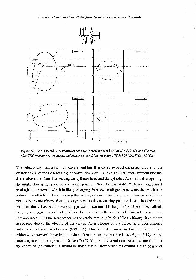
Experimental analysis of in-cylinder flows during intake and compression stroke
~~~----------------------~
vet1lcalposllionlmm] vmtical position (Iml]
Figure 6.17 '.' Measured velocity distributions along measurement line I at 450,540,630 and 675 DCA
after TDC of compression, arrows indicate conjectured flow structures (IVO: 360 DCA; IVC: 588 DCA)
The velocity distribution along measurement line IT gives a cross-section, perpendicular to the
cylinder axis, of the flow leaving the valve areas (see Figure 6.18). This measurement line lies
5 mm above the plane intersecting the cylinder head and the cylinder. At small valve opening,
the intake flow is not yet observed at this position. Nevertheless, at 405 °CA, a strong central
intake jet is observed, which is likely emerging from the small gap in between the two intake
valves. The effects of the air leaving the intake ports in a direction more or less parallel to the
port axes are not observed at this stage because the measuring position is still located in the
wake of the valve. As the valves approach maximum lift height (450 °CA), these effects
become apparent. Two direct jets have been added to the central jet. This inflow structure
remains intact until the later stages of the intake stroke (495-540 °CA), although its strength
is reduced due to the closing of the valves. After closure of the valve, an almost uniform
velocity distribution is observed (630°CA). This is likely caused by the tumbling motion
which was observed above from the data taken at measurement line I (see Figure 6.17). At the
later stages of the compression stroke (675 °CA), the only significant velocities are found at
the centre of the cylinder. It should be noted that all flow structures exhibit a high degree of
155

In-Cylinder Flow Analysis for Production-Type Internal-Combustion Engines
·~f8!-;-.S----------';C----------::
sr-------~------_,
-5: direct
I \ jets
r\\", ......... _ ..... -
-~~8'-:-.S------~'--------='------::!
i:\",,'-_____ --/\Y~ ____ //
-~~8L-.S------------":O----------,J
horizontalposition[mmj
_S·····----------.o---<"··~~···"-<>-·-··-----------'
-10
-~~8~.S---------!------------;-!
":1a'-:-.s------------":----------,J
sr-------~------_,
.. ~~---"'-----" ..... -.. --
-~8''-;-.S---------!-O---------::! horizonte.lpositiOll(mm)
Figure 6.18 '.' Measured velocity distributions along measurement line II at 405,450,495,540, 630
and 680 DCA after TDC of compression, dashed lines and arrows indicate conjectured flow structures
(IVO: 360 DCA; IVC: 588 DCA)
symmetry, throughout the intake and compression strokes. The observed plane of flow
symmetry approximately coincides with the plane of symmetry of the cylinder head.
The observations may lead to the believe that the two direct jets and the single central jet
induce a single tumbling motion, similar to the axi-symmetric model engine studied in
Section 3.3, that persists until the later stages of the compression stroke. However, the data
156

Experimental analysis of in-cylinder flows during intake and compression stroke
·:1s~.s-------:---------::
I f 0 __ ,
.......... ...... ~
·:1sL,-.s-------:o--------::! horilonlalposttlon[nm]
·:1sL,-.s-------:---------,-J
A ... ., ~.~+~ ......... ..
o _. ________ -
·~C=-.s-------::-o-------:-: horizonlaiposltJon{mrn)
Figure 6.19 '.' Measured velocity distributions along measurement line III at 450,540,585 and
630 DCA after TDC of compression, dashed lines and arrows indicate conjectured flow structures
(IVO: 360 DCA; IVC: 588 DCA)
taken at measurement line ill, which is half way between the TDC and the BDC piston
positions, suggest a much more complex flow structure, as indicated by Figure 6.19. Already
at the mid-stages of the intake stroke (450 °CA), steep velocity gradients are observed at this
position. The observed flow direction at the centre of the cylinder is opposite to that in the
outer regions. This indicates the existence of two counter-rotating swirling motions. These
structures persist well into the compression stroke (585°CA). Again, the flow structures
clearly indicate symmetry, similar to the observations made above. At the mid-stages of the
compression stroke (630°CA), the swirling motions have become much less apparent, but
that is likely due to the piston having almost reached the measurement line at this stage.
The indication that a single tumbling motion does not exists outside the symmetry plane is
confirmed by the velocity distributions found at axial measurement line IV, which is at the
centre of one of the presumed swirling motions (see Figure 6.20). Again, a strong intake jet is
observed close to the cylinder head, which emerges directly from the intake port. During the
second half of the intake stroke (495 °CA), a layered flow with steep gradients is observed
157

In-Cylinder Flow Analysis for Productioiz-Type Internal-Combustion Engines
direct intake jet
':tf:= j
verticalposition[rrmJ
_30L----=-_____ --==:..--___ _
v.=rticalposllionIrm'I]
Figure 6.20 '.' Measured velocity distributions along measurement line IV at 450,495,540,585,
630 and 675 DCA after TDC of compression, arrows indicate conjectured flow structures (IVO:
360 DCA; IVC: 588 DCA)
above the piston face. However, no subsequent tumbling motion is observed. Apparently,
tumble only exists at the symmetry plane (Figure 6.17). That tumbling motion is induced by
the central intake jet emerging from the gap in between the two valves, as seen in Figure 6.18.
The jets that emerge directly from the intake ports apparently induce two counter-rotating
swirling motions.
158

Experimental analysis of in-cylinder flows during intake and compression stroke
6.7 Conclusions and discussion
A dedicated optically-accessible engine was designed and built for the experimental
investigation of unsteady in-cylinder flow structures, as is described in Section 6.1. This
engine facilitates back-scattering LDV through a piston-based window. Although presently
operated and tested at motored conditions, the engine was designed to also allow for fired
operation. Through proper design, it was proven possible to apply oil-lubrication while the
generally-encountered problems of window and mirror fouling were largely minimised. The
present engine can be operated for several consecutive hours without cleaning. Moreover,
engine wear was seen to be minimal. Special positioning systems for the optics enable radial
and tangential velocity components to be measured throughout a major part of the combustion
chamber. Ti02 particles, generated as described in Section 4.2.3, were successfully applied as
scatterers for the LDV experiments.
Conducting in-cylinder velocity measurements with a back-scattering LDV configuration was
proven possible. The flow analyses given in Section 6.6 showed that much insight into the
temporal and spatial in-cylinder flow structures can already be gained from a relatively small
number of measurements. The observed flow structures are clearly not straightforward. The
three-dimensional nature of modem reciprocating engines implies the in-cylinder air motion
to be considerably more complex than, for instance, of the axi-symmetric model engine
(Section 3.3). Despite the insight gained from the experimental results, more data is needed to
draw definite conclusions. Such data may be obtained from additional LDV experiments.
Alternatively, multi-dimensional techniques such as PIV may be applied to check whether
flow descriptions that are constructed on the basis of the LDV results are correct. However,
practicable experiments can not reveal all flow details. Consequently, again a definite need
for validated computational methods exists in order to obtain a more complete flow
description. The experimental data obtained in the present investigation may already offer a
validation means for computational results. Ultimate validation should involve a larger data
set for the present and other operating conditions, such as operation at different engine speeds
and engine loads. The present investigations proved that such data can be obtained in a
quantitative and reliable manner with the test rig and experimental techniques used in this
study.
Unfortunately, the observed data rates were too low to allow for the discrimination of the
effects of turbulence and of cycle-to-cycle variation. An LDV set-up with scattered light
collection in forward or sideward direction is expected to yield much higher data rates.
Application of such a configuration puts considerable demands on the design of the engine.
However, small windows in the cylinder liner may be feasible and would not only facilitate
sideward light-collection, but additionally allow for LDV of axial velocity components.
Moreover, it allows for the application of an in-cylinder laser sheet in order to facilitate PIV
experiments. Alternatively, preliminary investigations on the feasible data rates with forward-
159

In-Cylinder Flow Analysis for Production-Type Internal-Combustion Engines
scattering could be analysed with a set-up involving a window in one of the three spark plug
holes of the cylinder head. This practise is recommended as the next step because its
realisation is relatively straightforward and it may already yield valuable information.
Although such a window would be very small, it is expected to enable forward-scattering
LDV along an axial line in the combustion chamber.
160

Concluding discussion
7. Concluding discussion
The objective of the present investigation was to contribute to the understanding of in
cylinder fluid motion in modern internal-combustion engines and to present further evidence
of the value of sophisticated experimental and computational techniques for engine research
and development. Below, the most important conclusions of this study are summarised and
recommendations for future investigations are presented. Finally, some closing remarks are
put forward.
Conclusions
Numerical simulations of the steady flow in an axi-symmetric rig and the unsteady flow in an
axi-symmetric model engine showed that steady-flow analysis can yield valuable insight into
the flow structures induced during the early stages of the intake stroke (Section 3.3). Such
steady-flow analyses can either be experimental or computational. Successful LDV
experiments were conducted on the steady flow in an engine flow rig for a modern four-valve
cylinder head at several combinations of valve-lift height and mass-flow rate (Section 5.2). A
computational method for the simulation of the three-dimensional steady flows in this engine
rig was thoroughly validated with the acquired experimental data (Section 5.4). It was
concluded that the computational method produces good predictions of the large-scale in
cylinder fluid motion, despite the associated assumptions, such as isotropic distribution of
turbulence. Comparison of the performances of the 'standard' k-c turbulence model and its
RNG and CHEN variants led to the conclusion that there exists no apparent reason to
abandon the standard model for the simulation of these flow types. It was demonstrated that
validated computational methods can be used for enlightening comparative studies of the
performance of different intake port designs (Section 5.5).
The flow structures induced during the early stages of the intake stroke are altered during the
remaining part of the intake stroke and during the compression stroke. This process is
essentially unsteady. For the experimental investigation of such unsteady flows, a production-
161

In-Cylinder Flow Analysisfor Production-Type Internal-Combustion Engines
type, optically-accessible, single-cylinder, spark-ignition engine was developed which
facilitates in-cylinder LDV at motored as well as fired conditions (Sections 6.1 to 6.3).
Through optimisation of the oil-lubrication systems and the seeding properties, window
fouling was minimised such that reliable experiments can be conducted during several hours
of operation without window cleaning. Successful in-cylinder and in-manifold velocity
measurements were conducted with a back-scattering LDV set-up (Sections 6.S and 6.6). It
was shown that the data acquired at a limited number of measuring positions can already
contribute to the understanding of the complex flow structures occurring in engines. This was
demonstrated by the finding that the investigated in-cylinder flow does not exhibit a
predominantly tumbling air motion, as might be expected for a symmetrical engine geometry
with two directed intake ports and a pent-roof combustion chamber. In fact, a combination of
tumble and two counter-rotating swirling motions was observed. Apart from adding to the
understanding of in-cylinder flows, the acquired experimental data can be used to validate
numerical simulations of these unsteady flows.
In general, the investigation of the steady and unsteady in-cylinder flows has shown that LDV
and CFD are powerful tools for modem engine research and development. These techniques
can offer insight into the flow that can not be given by less-sophisticated methods.
Recommendations
The present LDV experiments at the motored engine are merely preliminary. A larger data set
should be taken at the presently-considered conditions as well as at other conditions, such as
different engine speeds and engine loads. Such data would allow for a more elaborate analysis
of in-cylinder flow structures. However, the results of the LDV experiments for the engine
flow rigs as well as for the motored engine indicated that a high spatial measuring resolution
is required to allow for conclusive descriptions of the in-cylinder flow structures. A judicious
combination of LDV and a whole-field measuring technique, such as PIV, is considered ideal
for this purpose. Therefore, application of PIV to both the flow rig and the real engine is
recommended for future studies.
The demand for high spatial resolution, and the effort and cost involved with designing test
rigs and conducting reliable experiments, indicate a definite need for numerical simulations.
The value and validity of a computational method for the steady flows in engine rigs has been
shown in this thesis. The numerical simulation of the unsteady flow in the motored engine,
and its experimental validation with the acquired data, could not be completed within the
present investigation. It is recommended that this study is finished so that the accuracy of
such simulations can be assessed. A validated computational method can help to understand
how the complex flow structures, like the ones that were observed from the experimental
data, arise and develop during the engine cycle. Furthermore, comparison of numerical
162

Concluding discussion
simulations of the steady flow in the rigs and the unsteady flow during the intake stroke of the
real engine will allow for a further assessment of the value of steady-flow analysis at realistic
engine conditions.
Unfortunately, the data rates attained for the unsteady-flow measurements with the present
set-up are too low to allow for the discrimination of the effects of turbulence and cycle-to
cycle variation. Therefore, it is recommended that these effects are studied through
application of a forward-scattering LDV set-up, which is expected to yield much higher data
rates (Section 6.7).
Closure
The present investigation learns that LDV and CFD of the flow in realistic engine geometries
remain the domain of specialists. The costs and time involved to complete such analyses is
high. While there remains room for improvement and further validation, engine design
through application of these techniques is technically viable today and provides detailed
insight into the in-cylinder processes. It is not anticipated that CFD will ever replace
experiments, but rather that there will be an evolving blend of CFD and measurements. The
computational capability to fully resolve all relevant hydrodynamic length and time scales in
the engine, even without combustion and sprays, is not foreseen for the near future.
Continued work on modelling of turbulence, on improved computational methodologies, as
well as further automation of grid generation techniques for complex flow geometries will
allow for improved accuracy and a more efficient application of CFD.
Finally, it is important to bear in mind that experiments of complex physical systems are
subject to difficulties analogous to those experienced in computations. Experimental
diagnostics, as models, generally are developed and calibrated in simple, controllable
configurations. Application of highly sensitive techniques, such as LDV, on complex realistic
problems is never straightforward. Thus, in comparing computation and measurement of
flows in realistic engine configurations, it is appropriate to view the exercise as one of
reconciliation between computation and measurement rather than as one of validation of a
computational method.
163

In-Cylinder Flow Analysis for Production-Type Internal-Combustion Engines
164

References
References
Absil, L.H.J. (1995). Analysis of the laser Doppler measurement technique for application in turbulent flows,
dissertation, ISBN 90-5623-017-4, Delft University.
Adrian, R. (1983). Developments in laser techniques and applications to fluid dynamics: proceedings of the
international symposium, Adrian, R., Durao, D.F.G. and Durst, F. (eds.), Springer Verlag, Berlin.
Ahmadi-Befrui, B. and Gosman, A.D. (1989). Assessment of variants of the k-£ turbulence model for engine
flow applications, Int. J. Num. Meth. in Fluids, 9, pp.1073-1086.
Ahmadi-Befrui, B., Brandstiitter, W., Hofler, T., Pitcher, G. and Wigley, G. (1993). Driedimensionales
simulationsmodell zur berechnung der turbulenter luftbewegung in zylindern (i~ German),
Motortechnische Zeitschrift, 54, pp. 154-160.
Arcoumanis, C., Begleris, P., Gosman, A.D. and Whitelaw, J.H. (1986). Measurement and calculations of the
flow in a research Diesel engine, SAE paper 861563.
Arcoumanis, C., Bicen, A.F. and Whitelaw, J.H. (1983). Squish and swirl-squish interaction in motored model
engines, J. Fluids Eng., 105, pp. 104-112.
Arcoumanis, C. and Whitelaw, J.H. (1987). Fluid mechanics of internal combustion engines - a review,
proceedings Instn. Mech. Engrs., 201, no Cl.
Arcoumanis, C., Cossali, E., French B. and Whitelaw, J.H. (1988). Inlet valve flow generated by helical ports,
proceedings of 4th international symposium Applications of Laser Anemometry to Fluid Dynamics,
Lisbon, pp. 119-132.
Befrui, B.A. (1994). CFD simulation and comparison with measurement of steady flow in intake ports and
combustion chambers, International Symposium COMODIA 94, pp. 535-540.
Bendat, J.S. and Piersol, A.G. (1986). Random data, analysis and measurement procedures, ISBN 0-471-04000-
2, 2nd edition, John Wiley & Sons, New york.
Bicen, A.F. (1983). Air flow characteristics of model internal combustion engines, dissertation, University of
London.
Bicen, A.F., Vafidis, C. and Whitelaw, J.H. (1985). Steady and unsteady airflow through the intake valve of a
reciprocating engine, J. Fluids Eng., 107, pp. 413-420.
Bo, T., Clerides, D., Gosman, A.D. and Theodossopoulos, P. (1997). Prediction of the flow and spray processes
in an automobile DI Diesel engine, SAE paper 970882.
Bopp, S., Durst, F. and Tropea, C. (1990). In-cylinder velocity measurements with a mobile fiber optic LDA
system, SAE paper 900055.
Boussinesq, J. (1877). Essai sui la theorie des eaux courantes (in French), Mem. Presentes Acad. Sci., 23, p. 46,
Paris.
Boussinesq, J. (1903). Theorie analytique de la chaleur, vol. 2., Gauthier-Villars, Paris.
165

In-Cylinder Flow Analysis for Production-Type Internal-Combustion Engines
Bradley, D. (1992). How fast can we burn?, twenty-fourth symposium on combustion, Pittsburg, ISBN 0082-
0784, pp. 247-278.
Brandstatter, W., Johns, RJ.R. and Wigley, G. (1985). The effect of inlet port geometry on in-cylinder flow
structure, SAE paper 850499.
Briicker, Ch. (1997). High-speed video: an upcoming chance for time-resolved 3-D velocimetry based on light
sheet tomography, proceedings of the 7th International Conference on Laser Anemometry - Advances
and Applications, Karlsruhe, pp. 427-435.
Caspersen, C. (1992). The enhanced burst spectrum analyzer, Dantec Information, no. 11, pp. 17-20.
Chatfield, C. (1983). Statistics for technology - a course in applied statistics, third edition, ISBN 0 412 25340 2,
Chapman and Hall, London.
Chen, Y.S., and Kim, S.W. (1987). Computation of turbulent flows using an extended k-E turbulence closure
model, NASA CR-179204.
Clayton, R.P. (1994). The calculation of complex turbulent flows with computational fluid dynamics, Master's
thesis, Imperial College, London.
Computational Dynamics (1996). STAR-CD manuals - version 3.0, Computational Dynamics Limited, London.
Courant, R., Isaacson, E. and Rees, M. (1952). On the solution of non-linear hyperbolic differential equations by
finite differences, Comm. Pure Appl. Math., 5, p. 243.
Damk6hler, G. (1940). Z. elektrochem. angew. phys. chern. (in German), 46, p. 601 (English translation: Techn.
memo. nat. advis. comm. aeronaut, Wash., p. 1112, 1947)
Delphi (1996). Emissions standards passanger cars worldwide, Delphi technical centre, Luxembourg.
Demirdzic, I. And Peric, M. (1988). Space conservation law in finite volume calculations of fluid flow, Int. 1.
Num. Meth. Fluids, 8, pp. 1037-1050.
Dimopoulos, P. and Boulouchos, K. (1997). Turbulent flow field characteristics in a motored reciprocating
engine, SAE paper 972833.
Dogge, E. (1996). Toepassing van een hogere orde discretisatieschema: ULTRA-QUICKER (in Dutch), internal
repport WOC-WET 96.040, Eindhoven University of Technology, Eindhoven.
EI Tahry, S.H. (1983). k-£ equation for compressible reciprocating engine flows, AIAA 1. Energy, 7, No.4, pp.
345-353.
EI Tahry, S.H. (1985a). Application of a Reynolds stress model to engine-like flow calculations, transactions of
ASME, 107, pp. 444-450.
El Tahry, S.H. (1985b). A comparison of three turbulence models in engine-like geometries, International
Symposium COMODIA '85, pp. 203-213.
Exxon (1998). Paramins postscript july 1998, Exxon chemical limited.
Fell, S. (1997). Some general considerations for calculating the flow around a car, proceedings 6th STAR-CD
user conference, London.
Gindele, J., Kech, J.M., Scholl, D.M. and Spicher, U. 0997). Time resolved investigation of unsteady flow
inside inlet manifolds and characterization of inlet flow behaviour, SAE paper 972828.
Godrie, P. and Zellat, M. (1994). Simulation of flow field generated by intake port-valve-cylinder configurations
- comparison with measurements and applications, SAE paper 940521.
Gosman, AD., Pun, W.M., Runchal, AK., Spalding, D.B., and Wolfstein, M. (1969). Heat and mass transfer in
recirculating flows, Academic Press, London.
Gosman, AD. (1985a). Multidimensional modeling of cold flows and turbulence in reciprocating engines, SAE
paper 850344.
Gosman, AD. (1985b). Computer modeling of flow and heat transfer in engines - progress and prospects,
proceedings of International Symposium COMODIA '85, Tokyo.
Grosjean, N., Graftieaux, L., Michard, M., Hiibner, W., Tropea, C. and Volkert, J. (1997). Combining LDA and
PIV for turbulence measurements in unsteady swirling flows, Laboratoire de Mechanique des Fluides et
d'Acoustic, France.
166

References
Hallback, M., Johansson, AV. and Burden, AD. (1996). The basics of turbulence modelling, in: Turbulence and
transition modelling, Hallback et al. (eds.), ISBN 0-7923-4060-4, Kluwer Academic Publishers,
Dordrecht.
Hascher, H.G., Jaffri, K., Novak, M., Lee, K., Schock, H., Bonne, M. and Keller, P. (1997). An evaluation of
turbulent kinetic energy for the in-cylinder flow of a four-valve 3.51 SI engine using 3-D LDV
measurements, SAE paper 970793.
Hassid, S., and Poreh, M. (1975). A turbulent energy dissipation model for flows with drag reduction, J. Fluids
Eng., 100, pp. 107-112.
Hayworth, D.C. and Jansen, K. (1996). LES on unstructured deforming meshes: towards reciprocating IC
engines, Proceedings of the summer program 1996, Center for turbulence research, pp. 329-346
Heywood, J.B. (1988). Internal combustion engine fundamentals, ISBN 0-07-028637-X, McGraw-Hill, New
York.
Hinze, P.O. (1975). Turbulence, 2nd edition, McGraw-Hill, New York.
Hirsch, Ch. (1988a). Numerical computation of internal and external flows - Vol. 1 Fundamentals of numerical
discretization, ISBN 0 471917621, John Wiley and Sons, New York.
Hirsch, Ch. (1988b). Numerical computation of internal and external flows - Vol. 2 Computational methods for
inviscid and viscous flows, ISBN 0 471923516, John Wiley and Sons, New York.
Hofler, T. and Wigley, G. (1993). Experimental investigation and three-dimensional calculation of the steady in
cylinder flow generated by a helical port, Turbulence, Heat and Mass Transfer 1, Begell House, New
York, pp. 553-558.
Hofler, T., Pitcher, G. and Wigley, G. (1993). A comparison of Diesel engine inlet valve flows under steady
state and motoring conditions, proceedings of the 5th International Conference on Laser Anemometry -
Advances and Applications, pp. 737-744.
Hu, Z., Vafidis, c., Whitelaw, J.H., Chapman, J. and Head, R.A (1992). Correlation between in-cylinder flow,
performance and emissions characteristics of a Rover pentroof four-valve engine, IMechE C448/026,
pp. 157-164
Issa, R.I. (1986). Solution of the implicitly discretised fluid flow equations by operator-splitting, J. Compo Phys.,
62, pp. 40-65.
Issa, R.I., Gosman, AD., and Watkins, AP. (1986). The computation of compressible and incompressible
recirculating flows by a non-iterative implicit scheme, J. Compo Phys., 62, pp. 66-82.
Issa, R.I., Ahmadi-Befrui, B., Beshay, K., and Gosman, AD. (1991). Solution of the implicitly discretised
reacting flow equations by operator-splitting, J. Compo Phys., 93, pp. 388-410.
Jayatilleka, c.L. (1969). The influence of Prandtl number and surface roughness on the resistance of the laminar
sub-layer to momentum and heat transfer, Progr. Heat and Mass Transfer, 1, pp. 193-330.
Jones, W.P. (1980). Models for turbulent flows with variable density and combustion. In: Prediction methods for
turbulent flow, Kollman, W. (ed.), Hemishere, Washington, D.C.
Jovic, S. (1996). An experimental study of a separated/reattached flow behind a backward-facing step -
Reh=37,000, NASA Technical Memoradum 110384, NASA, Moffett Field.
Jovic, S. and Driver, D.M. (1994). Backward-facing step measurements at low Reynolds number, Reh=5000,
NASA Technical Memorandum 108807, NASA, Moffett Field.
Khalighi, B. Haworth, D.C. and Hubler, M.S. (1994). Multidimensional port-and-in-cylinder flow calculations
and flow visualisation study in an internal combustion engine with different intake configurations, SAE
paper 941871.
Khalighi, B., EI Tahry, S.H., Haworth, D.C. and Hubler, M.S. (1995). Computation and measurement of flow
and combustion in a four-valve engine with intake variations, SAE paper 950287.
Kolmogorov, AN. (1941). The local structure of turbulence in incompressible flow for very large Reynolds
numbers, Compt. Rend. Acad. Sci. URRS, 30, p.31.
Krebs, H. (1986). Glasfaser-Iaser-doppler-anemometer fUr messungen in verbrennungs-motoren (in German),
dissertation, University of Erlangen-Nurnberg.
167

In-Cylinder Flow Analysis for Production-Type Internal-Combustion Engines
Krlls, H.W. (1993a). Upstream influence of the impulse swirl meter, internal report 55310-93061, DAF Trucks
B.V., Eindhoven.
Krlls, H.W. (1993b). Numerical simulation and experimental verification of DI Diesel intake port designs,
proceedings 4th Int. EAEC conference, Strasbourg.
Lading, L. (1987). Spectrum analysis of LDA signals and postprocessing with a PC computer, proceedings of
ISL conference: The use of computers in laser velocimetry.
Lading, L., Wigley, G. and Buchhave, P. (1994) Optical diagnostics for flow processes, ISBN 0-306-44817-3,
Plenum Press, New York.
Launder, B.E. (1989). Second-moment closure: present ... and future?, Int. J. Heat and Fluid Flow, 10, pp. 282-
300.
Launder, B.E., and Spalding, D.B. (1974). The numerical computation of turbulent flow, Compo Meth. Appl.
Mech. Eng., 3, p. 269.
Le, H. and Moin, P. (1992). Direct numerical simulation of turbulent flow over a backward-facing step, Annual
Research Briefs 1992, Center for Turbulence Research, Stanford, pp. 161-173.
Lea, C.J. and Watkins, AP. (1997). Differential stress modelling of turbulent flows in model reciprocating
engines, Proc. Instn. Mech. Engrs., 211, part D, pp. 59-77.
Leonard, B.P. (1979). A stable and accurate convective modelling procedure based on quadratic upstream
interpolation, Compo Meth. Appl. Mech. Eng., 19, pp. 59-98.
Leonard, B.P. and Mokhtari, S. (1990). Beyond first-order upwinding: The ULTRA-SHARP alternative for non
oscillatory steady-state simulation of convection, Int. J. Num. Meth. Eng., 30, pp. 729-766.
Leonard, B.P. (1991). The ULTIMATE conservative difference scheme applied to unsteady one-dimensional
advection, Compo Meth. Appl. Mech. Eng., 88, pp. 17-74.
Lesieur, M. (1990). Turbulence in fluids, second revised edition, ISBN 0-7923-0645-7, Kluwer Academic
Publishers, Dordrecht.
Liou, T.-M., Hall, M., Santavicca, D.A and Bracco, F.V. (1984). Laser Doppler velocimetry measurements in
valved and ported engines, SAE paper 840375.
Limbach, S. (1997). Multi-dimensional computation of transient convective heat transfer: application to a
reciprocating engine, dissertation, Technischen UniversWit Graz.
Lorenz,M. and Prescher K. (1990). Cycle resolved LDV measurements on a fired SI-engine at high data rates
using a conventional modular LDV -system, SAE paper 900054.
Maanen, R.E. van (1993). Signaalprocessoren en signaalverwerking voor laser-Doppler anemometrie (in Dutch),
contribution to the Burgers Centre summerschool, Delft University of Technology, Delft.
Merzkirch, W. (1974). Flow visualisation, second edition, ISBN 0-12-491351-2, Academic Press Inc LTD.,
London.
Mie, G. (1908). Beitrage zur optik treiber medien (in German), Ann. der Physik, 4, p. 37:881.
Morse, AP., Whitelaw, J.H. and Yianneskis, M. (1979). Turbulent flow measurements by laser-Doppler
anemometry in motored piston-cylinder assemblies, transactions of the ASME, 101.
Navier, M (1827). Memoire sur les lois du movement de fluides, Mem. de l'Acad. de Sci., 6, pp. 389-416.
Nieuwstadt, F.T.M. (1992). Turbulentie: inleiding in de theorie en toepassing van turbulente stromingen (in
Dutch), ISBN 90-5041-028-6, Epsilon uitgaven, Utrecht.
Nijkamp, P. (1995). Scanning the transportation future, a long-term scenario approach, proceedings of
international symposium Concepts 2020, TNO road-vehicles research institute, Delft
Nikuradse, J. (1932). Gesetzmassigkeit der turbulenten stromung in glatten rohren, Furschg. Arb. Int.-Wes., 356.
Norris, L.H., and Reynolds, W.e. (1975). Turbulent channel flow with a moving wavy boundary, Report No.
FM-lO, Department of Mechanical Engineering, Stanford University, USA
Ntone F. and Zehr, R.L. (1993). Multidimensional fluid flow calculations in Diesel engine exhaust valve-port
geometries, SAE paper 930073.
Oberbeck, A (1879). Uber die warmeleitung der flllBigkeiten bei berllcksichtigung der stromungen infolge von
temperaturdifferenzen (in German), Annalen der Physik und Chemie, 7:271-292.
168

References
Patankar, S.V., and Spalding, D.B. (1972). A calculation procedure for heat, mass and momentum in three
dimensional parabolic flows, Int. J. Heat Mass Transfer, 15.
Patankar, S.V. (1980). Numerical heat transfer and fluid flow, ISBN Hemisphere, Washington, D.e.
Pinchon, P. (1990). Modelling of fluid dynamics and combustion in piton engines, International Symposium
COMODIA '90, pp. 31-47.
Piomelli, U. and Chasnov, J.R. (1996). Large-eddy simulations: theory and applications, in: Turbulence and
transition modelling, Hallback et al. (eds.), ISBN 0-7923-4060-4, Kluwer Academic Publishers,
Dordrecht.
Prandtl, L. (1925). Bericht uber untersuchungen zur ausgebildeten turbulenz, ZAMM, 5, p.136.
Press, W.H., Teukolsky, S.A., Vetterling, W.T., and Flannery, B.P. (1992). Numerical recipes in Fortran - the art
of scientific computing, second edition, ISBN 0 521430640, Cambridge University Press, Cambridge.
Rask, R.B. (1979). Laser Doppler anemometer measurements in an internal combustion engine, SAE paper
790094.
Riethmuller, M. (1977). Laser Doppler Velocimetry, in: Measurement of unsteady fluid dynamic phenomena,
B.E. Richards (ed.), Hemisphere publishing corporation, pp. 163-187.
Roach, P.J. (1972). Computational fluid dynamics, ISBN 0-913478-05-9, Hermosa Publishers, Albuquerque.
Rodi, W. (1979). Influence of buoyancy and rotation on equations for turbulent length scale, Proc. 2nd symp. on
turbulent shear flows.
Ruck, B. (1990). Lasermethoden in der stromungsmesstechnik (in German), ISBN 3-921 681-01-4, AT
Fachverlag GmbH, Stuttgart.
Rudd, M.J. (1969). A new theoretical model for the laser Doppler meter, J. Phys. E. Sci. Instrum., 2, pp. 723-
726.
Runchal, AK. (1987). CONDIF: A modified central-differencing scheme for convective flows, Int. J. Num.
Meth. Eng., 24, pp. 1593-1608.
Sanders, J.P.H. (1993). Scalar transport and flamelet modelling in turbulent jet diffusion flames, PhD thesis,
ISBN 9038601433, Eindhoven University of Technology.
Schafer, F., Barte, S. and Bulla, M. (1997). Geometrische zusammenhange an zylinderkopfen (in German),
Motortechnische Zeitschrift, 58, pp. 384-391.
Schlichting, H. (1979). Boundary layer theory, ISBN 0-07-055334-3, McGraw-Hill, New York.
Semenov, E.S. (1958). Device for measuring the turbulence in piston engines, Instrum. Exp. Tech., 1, pp. 102-
111.
Spalding, D.B. (1972). A novel finite difference formulation for differential expressions involving both first and
second derivatives, Int. J. Numer. Methods in Engineering, 4, pp. 551-559.
Speziale, e.G. (1987). On non-linear k-l and k-£ models of turbulence, J. Fluid Mech., 178, pp. 459-475.
Stokes, G.G. (1845). On the theories of internal friction of fluids in motion, Trans. Cambro Phil. Soc., 8, pp.
287-305.
Stone, R. (1992). Introduction to internal combustion engines, second edition, ISBN 0-333-55084-6, The
MacMillan Press, London.
Theunissen, AB.M. (1994). LDA-metingen stationaire stromingen (in Dutch), internal report woc/vtlr/94.76,
Eindhoven University of Technology.
Tu, J.Y. and Fuchs, L. (1992). Three-dimensional unsteady flow calculations in both intake port and combustion
chamber, AIAA paper 92-0833, 30th Aerospace Sciences Meeting, Reno.
Urlaub, A (1995). Verbrenningsmotoren - grundlagen, verfahrentechnik, konstruktion (in German), ISBN 3-
540-58194-4, Springer-Verlag, Berlin.
Vafidis, C. (1984). Influence of induction swirl and piston configuration on air flow in a four-stroke model
engine, proceedings Instn. Mech. Engrs., 198C, no. 8.
Valentino, G., Corcione, F.E. and Seccia, G. (1997). Integral and micro time scales estimate in a DJ. Diesel
engine, SAE paper 971678.
169

In-Cylinder Flow Analysis for Production-Type Internal-Combustion Engines
Van den Heuvel, S.L., Van Steenhoven, AA and Baert, RS.G. (1997). Three-dimensional calculations and
laser velocimetry validation of steady-state port-valve-cylinder flows, proceedings of the 7th
International Conference on Laser Anemometry - Advances and Applications, Karlsruhe, pp. 245-252.
Van den Hurk, O.J. (1996). LDA-snelheidsmetingen vergeleken met simulaties bij stationair doorgeblazen
cilinderkop (in Dutch), MSc. thesis, WOC-WET 96.019, Eindhoven University of Technology.
Van Driest, E.R (1956). On turbulent flow near a wall, J. Aeronaut. Science, 23, pp. 1007-1011.
Van Peer, B.AR van (1997). Seeding voor LDA in het bijzonder voor toepassing in verbrandingsmotoren (in
Dutch), thesis WOC-WET 97017, Eindhoven University of Technology.
Versteeg, H.K. and Malalasekera, W. (1995). An introduction to computational fluid dynamics, the finite volume
method, ISBN 0-582-21884-5, Longman Group limited, Harlow.
Vogel, J.e. and Eaton, J.K. (1985). Combined heat transfer and fluid dynamic measurements downstream of a
backward-facing step, J. Heat Trans., 107, pp. 922-929.
Warsi, Z.V.A (1981). Conservation form ofthe Navier Stokes equations in general nonsteady coordinates, AIAA
J., 19, pp. 240-242.
Watkins, AP., Kanellakopoulos, P. and Lea, e.J. (1990). An assessment of discretisation schemes and
turbulence models for in-cylinder flows, proceedings of International Symposium COMODIA '90, pp.
499-504.
Wigley, G. (1987). Laser anemometer techniques in internal combustion engines, second International
Conference on Laser Anemometry - Advances and Applications, Glasgow, pp. 1-28.
Witze, P.O. (1977). Measurements of the spatial distribution and engine speed dependence of turbulent air
motion in an IC engine, SAE paper 770220.
Witze, P.O. (1980). A critical comparison of hot-wire anemometry and laser Doppler velocimetry for IC engine
applications, SAE paper 800132.
Witze, P.O. and Baritaud, T.A (1986). Particle seeding for Mie scattering measurements in combusting flows,
third international symposium on applications of laser anemometry to fluid dynamics, Lisbon.
Wolfstein, M. (1969). The velocity and temperature distribution in one-dimensional flow with turbulence
augmentation and pressure gradient, Int. J. Heat Mass Transfer, 12, pp. 301-318.
Yakhot, V., and Orszag, S.A (1986). Renormalization group analysis of turbulence - I: Basic theory, J.
Scientific Computing, 1. pp. 1-51.
Yakhot, V., Orszag, S.A, Thangam, S., Gatski, T.B., and Speziale, e.G. (1992). Development of turbulence
models for shear flows by a double expansion technique, Phys. Fluids, A4, 7, pp. 1510-1520.
Yeh, Y. and Cummins, H.Z. (1964). Localized flow measurements with an He-Ne laser spectrometer, Appl.
Phys. Letters, 4, p. 176.
Yokota, H., Sugihara, H., Kakegawa, T., Aoyagi, Y. and Joko, 1. (1993). An experimental study of in-cylinder
air motion in a 4 valves per cylinder engine - an invesitigation of swirl evaluating methods under steady
state flow conditions, JSAE Review 9303438, 14, no. 2.
Yoo, S.-e., Lee, K.L., Novak, M., Schock, H. and Keller, P. (1995). 3-D LDV measurement of in-cylinder air
flow in a 3.51 four-valve SI engine, SAE 950648.
170

Appendices
171

In-Cylinder Flow Analysis for Production-Type Internal-Combustion Engines
172

Appendix A
A. Turbulence modelling
Three different k-E turbulence models were applied in the present investigation: the 'standard'
model, and its Renormalisation Group (RNG) and CHEN variants. Below, the essence of k-E
turbulence models is described. Subsequently, the individual model equations and their
specific properties are presented.
Constitutive relations for turbulent stresses and heat fluxes
The k-E modelling assumes that the turbulent Reynolds stresses 'Ci7 and the turbulent scalar
fluxes are linked to the ensemble-averaged flow properties in an analogous fashion to their
laminar counterparts, the viscous stresses 'Cij (Launder and Spalding, 1974):
(A.1)
- f.1 dh -pu~h'=--t --
] (}h,t d Xj
(A.2)
where the turbulent Prandtl number (}h,t is defined as f.1t·cp/kt, with k t being the turbulent
thermal conductivity coefficient. The turbulent kinetic energy k is defined as
u~u~ k=_'_' - 2 . (A.3)
The last term in equation A.l is introduced to ensure consistency with equation A.3 for i=j,
since 'Ci~ is equal to minus twice the turbulent kinetic energy per unit volume pk (Hirsch,
1988b).
173

In-Cylinder Flow Analysis for Production-Type Internal-Combustion Engines
The quantity J.lt represents the so-called turbulent viscosity. The turbulent Reynolds stresses
and turbulent heat fluxes are modelled by gradient-diffusion expressions. Hence, they are
described as additional diffusion transport processes, with /1t being the turbulent diffusion
coefficient. The idea of turbulent viscosity is based on the notion of the momentum transfer in
a turbulent flow being dominated by the mixing caused by the large energy-containing
turbulent eddies. The first ideas along these lines seem to have been proposed by Boussinesq
(1877). Therefore, this approach is known as the Boussinesq hypothesis. The turbulent
viscosity J.lt is linked to k and £ by assuming proportionality to the product of a characteristic
velocity fluctuation and length scale of the energy containing motions. These scales are
defined as U == k 1/2 and L == k 3/2/£ , respectively. Hence, the turbulent viscosity is given by
CJ1pe /1(=--- ,
£
(A A)
where CJ.l is an empirical model coefficient. This is an isotropic entity, which implies that all
modelling based on the constitutive relations of equations A.l and A.2 can not describe
anisotropy of turbulence.
The turbulent energy dissipation rate £ is modelled as (Launder and Spalding, 1974;
Nieuwstadt, 1992; Yakhot et aI., 1992):
(A.S)
Standard k-e model equations
The 'standard' k-£ model (Launder and Spalding, 1974) is used in this study in a high
Reynolds number form and in conjunction with algebraic 'law-of-the-wall' representations of
flow properties within boundary layers, as is discussed in Appendix B. Basically, the
derivation of transport equations for turbulence energy k and turbulence dissipation rate £ is
based on the Navier-Stokes equation for the velocity fluctuations u:. These equations are
obtained by subtracting the Reynolds-averaged Navier-Stokes equations from the full Navier
Stokes equations. The transport equations for k and £ can then be found by application of
equations A.3 and A.S.
174

Appendix A
Cil 1]0 f3
0.09 1.0 1.22 1.44 1.92 -0.33
Table A.I '.' Empirical coefficients appliedfor the standard k-e turbulence model
The equation that is applied for compressible flows in the present investigations is given by
EI Tahry (1983):
d (-) d (_ /left d k J - 2 ( d li; -) d li; :l P k +-;-- PUj k ---;-- = /It P- P E-- /It -;-+ P k -;- , at aX. (Jk aX. ~ '--v-' 3 aX. aX. '--.r------' \ J J, T4 15 \ I I ,
1j T2 :"'T3 ';6
where the turbulence production P is defined as
duo P==2s .. --1 ,
IJ dXj
while (Jk is an empirical coefficient. The effective viscosity /left is defined as
/left == /l + /It
(A.6)
(A.7)
(A.8)
For high Reynolds numbers, this effective viscosity is dominated by the turbulent viscosity /l('
given by equation A.4. Transport of the turbulence dissipation rate E follows from:
d (-) d ( /left dE J - pE +-- pUjE---- = dt dX j (Je dX j '--y-J \ I
T, v 1 ~-15
(A.9)
where (Je, Ce], Cel and Ce4 are empirical coefficients whose values are given in Table A.l,
along with Cil and (Jk.
The first term T 1 of both the equations A.6 and A.9 represents the rate of change of k or E.
Terms T 2 and T 3 account for transport of k or E by convection and diffusion, respectively. The
first term on the right-hand side of both equations, T 4, gives the production rate of k or E by
shear and normal stresses, which is fed by macroscale destruction of the mean flow kinetic
175

In-Cylinder Flow Analysis for Production-Type Internal-Combustion Engines
energy. The negative-signed term Ts represents the destruction rate of k or e through
microscale viscous dissipation. Production and destruction of turbulent kinetic energy k are
always closely linked. The dissipation rate e is large where production of k is large. The
model equation for e assumes that its production and destruction terms are proportional to
those of the k-equation. Adoption of such forms ensures that e increases rapidly when k
increases rapidly and that it decreases sufficiently fast to avoid non-physical negative values
of turbulent kinetic energy if k decreases (Versteeg and Malalasekera, 1995). The factor elk,
which represents the inverse of the dissipation time scale, renders the production and
destruction terms dimensionally correct in the e-equation. The final term, T 6, describes
amplification or attenuation due to compressibility effects.
RNG k-€ model equations
The RNG turbulence model is based on the work of Yakhot and Orszag (1986) and
Yakhot et. al. (1993). The procedure is as follows: first, a narrow band of the smallest energy
containing eddies is removed by expressing their effects in terms of larger scale motions and
an increased effective viscosity. As a result, the effective Reynolds number of the system
decreases. This process is repeated in an iterative manner, so that more and more scales of
motion are removed from the dynamics to a point where the remaining scales are all
resolvable. The removal of only the smallest scales gives rise to so-called subgrid-scale
models, in a similar fashion to LES. In the limit, as successively-larger scales are removed, a
model equivalent to the standard k-e model is recovered.
Through the scale-elimination procedure, RNG theory develops an equation for the variation
of the effective viscosity J1eff with the eddy length scale l. Thus, a formula is obtained with
which J1eff(l) is interpolated between the molecular viscosity J1 for the Kolmogorov
microscale 1 = 11 and the high-Reynolds-number limit of 1 = L» 11. The detailed mathematics
of the RNG k-e model is highly abstruse. Here, only the resulting model equations are quoted.
The RNG transport equation of turbulence energy is equal to that of the standard k-e model as
given by equation A.6. Transport of turbulence dissipation rate is as follows:
(A.10)
176

Appendix A
CIl 1]0 f3 0.0085 0.719 0.719 1.42 1.68 -0.387 4.38 0.012
Table A.2 '.' Empirical coefficients applied in the RNG k-E turbulence model
where 1]0 and f3 are empirical model constants given in Table A.2. The non-dimensional strain
rate 1] is defined as
k 1] == S- ,
c
S == ~2sij sij .
(A. 11)
(A.12)
Apart from the values of the model constants, which are also given in Table A.2, terms T 1 to
T 6 in equation A.l 0 are identical to those of the c-equation of the standard model. Notable
about the RNG derivation is that the values of the constants are calculated explicitly, whereas
the constants of the standard model have an empirical nature.
The additional last term in the dissipation rate equation, compared to the standard k-c model,
represents the effect of mean flow distortion on c (Rodi, 1979) and, in the form written in
equation A.l 0, it may be interpreted as an addition to term T 5. Indeed, in regions of small
strain rate 1], this term tends to increase the destruction rate of c. Nevertheless, /leff is still
typically smaller than its value in the standard theory due to the lower value of Cel • In regions
'of large strain rate, the sign of term T 7 is changed and its effect is one of increased production
rate of c, which becomes more apparent when it is rewritten in a similar fashion to production
term T4:
(A. 13)
As a consequence, the effective viscosity /leff, as given by equation AA, is decreased even
more. This feature of the RNG model may allow for an improved prediction of flow
separation and recirculation, which are prominent phenomena occurring in in-cylinder engine
flows. The model, as originally proposed, does not take explicit account of compressibility
effects. However, in the presently-applied modelling these effects are modelled as in the
standard k-c model.
177

In-Cylinder Flow Analysis for Production-Type Internal-Combustion Engines
CII 110 f3 0.09 0.75 1.15 1.15 1.9 -0.4 0.25
Table A.3 '.' Empirical coefficients applied in the CHEN k-t: turbulence model
CHEN's k-£ model equations
The so-called CHEN k-£ model is based on the work of Chen and Kim (1987). The
dissipation time scale, kl£, is the only turbulence time scale used in closing the £-equation of
the standard k-£ model. In Chen's model, the production range time scale, pP / J.l1k , as well
as the dissipation time scale, are used in closing the £-equation. This additional time scale
should allow the transfer mechanism of turbulence energy to respond to the mean strain rate
more effectively. This has resulted in an additional term, T 7, in the £ equation:
(A. 14)
where CE5 is an additional empirical coefficient, which is given in Table A.3 along with the
other model constants. Again, compressibility effects are modelled as in the standard k-£
model.
Terms 1 to 6 are again similar to the corresponding terms in the standard model equations.
The net effect of term T 7 is to enhance turbulent energy dissipation when the turbulence
production rate is large. This expression represents the energy transfer rate from large-scale
turbulence to small-scale turbulence controlled by both the dissipation rate time scale and the
production range time scale, as becomes more obvious when it is again written in a similar
fashion to term T 4:
(A. 15)
178

Appendix B
B. Modelling of near-wall region
For the discussion of the flow model in the near-wall region, first, non-dimensional quantities
that characterise flow properties within the boundary layer are introduced. The non
dimensional distance normal to the wall, y +, is defined as
+ PUr y =-y , (B.1) /1
where y is the normal distance to the wall. The so-called friction velocity U1: is given by
U ={:w r . p
(B.2)
The wall shear stress 'l"w can be written as
(B.3)
where /1t is the turbulent viscosity as given in equation AA. Under the assumption of one
dimensional equilibrium flow in the boundary layer, the local turbulence production rate is
balanced by the local dissipation rate. Hence, terms T 4 and T 5 of the k-equation A.6 are equal.
Moreover, only a single non-zero shear stress 'l"ij exists, which is approximately constant
throughout the boundary layer and, therefore, equal to the wall shear stress 'l"w. It can be
shown that the turbulence kinetic energy k, in its non-dimensional form, is then given by
kp , where k+ =- (BA)
'l"w
179

In-Cylinder Flow Analysis for Production-Type Internal-Combustion Engines
When substituting these expressions into equation B.l, the non-dimensional distance to the
wall can be rewritten as
pC1I4.jk Y y+=_--=-J1 __ _ f.1
(B.5)
In accordance with equation B.l, the non-dimensional velocity u + and temperature rare
defined as
, and
T+ = p(T-Tw)u"cp
FT,w
(B.6)
(B.7)
where u is the tangential fluid velocity, Uw is the wall velocity, which allows for the
representation of moving walls, Tw is the wall temperature and FT,w is the wall heat flux.
In the present investigation, so-called wall-function modelling is applied, which prescribes the
velocity and temperature distributions in the near-wall region. The expressions giving the
velocity distributions in terms of the normal distance y +, commonly known as the law of the
wall, are given by (Launder and Spalding, 1974):
(B.8)
A value of 9.0 was assigned to the profile shape factor E, whereas the 'von Karman'
coefficient K: is 0.42, 0.4 and 0.415 for the standard k-£ model and the RNG and CHEN
variants, respectively. In the wall-function approach, the buffer layer (Schlichting, 1979) is
usually not taken into account. The value of y: is defined as that distance from the wall at
which the linear velocity profile of the laminar sublayer (f.1t«)1) meets the logarithmic
profile of the fully turbulent inertial sublayer ()1t» )1). Hence, it must satisfy the equation:
(B.9)
180

Appendix B
Temperature distributions in boundary layers are given by:
(B.10)
where u+ is given by equation B.8, (JT (=f.1·cpITT; TT is the thermal conductivity) is the
molecular Prandtl number and (Jr.t is the turbulent Prandtl number. Finally, P is a non
dimensional sub-layer resistance factor dependent on the ratio of the molecular and the
turbulent Prandtl numbers given, for impermeable, smooth walls, by Jayatilleka (1969).
181

In-Cylinder Flow Analysis for Production-Type Internal-Combustion Engines
182

Appendix C
c. Basic principles of Laser-Doppler
Velocimetry
The experiments presented in Chapters 5 and 6 involve laser-Doppler velocimetry (LDV).
The specific application of this measuring technique to engines is addressed in Chapter 4. In
this appendix, its basic principles are described. First the mere essence of LDV is discussed:
the Doppler effect. Subsequently, the dual-beam method, the so-called fringe model, which is
helpful for understanding LDV, and signal characteristics are briefly explained. Finally, a
method to prevent directional ambiguity is described.
Doppler effect
As the name indicates, the basic physical principle involved in LDV is the Doppler effect. In
LDV the change of frequency of an incident laser beam is caused by the movement of small
particles scattering the light. A laser is used as the light source because it generates coherent,
monochromatic light waves. Furthermore, a laser can provide a light beam so intense that
even micron-sized particles scatter measurable amounts of radiation. Figure C.l shows a
particle, moving at velocity v, which is illuminated by a laser beam of frequency fi and
wavelength Il directed along unit vector ei • A detector, located in the direction of unit vector
es ' will receive scattered light of frequency is which, as a result of the Doppler effect, differs
from that of the incident beam. This frequency difference is firstly caused by the particle
having a velocity component in the direction of the beam causing it to receive the wavefronts
at a faster or slower rate thanA Secondly, the particle has a velocity component relative to the
detector which causes either compression or stretching of the wavefronts as the particle
scatters the wave in the direction of the detector. The frequency of the scattered radiation
received by the detector can be written as
(C.I)
183

In-Cylinder Flow Analysis for Production-Type Internal-Combustion Engines
detector
Figure C.l '.' Operating principle of LDV: a particle moving at velocity v, illuminated by a laser beam with frequency fi.
Since the particle velocity Ivl is usually much smaller than the speed of light e Ivl « c), the
Doppler shift fD, which is defined as the difference between the frequency of the scattered
radiation and that of the incident radiation, can be approximated by
ec.2)
Expression C.2 indicates that the Doppler shift depends linearly on the velocity of the
scattering particle, which is one of the favourable features of LDV. The Doppler shift is
furthermore determined by the scattering geometry, i.e. by the angle between the wave source
and the detector. The geometric layout is defined by the angles CfJ and a, which denote the
scattering angle and the angle between the velocity vector and the vector (e", - ei ), as
indicated in Figure C.1. The Doppler shift can also be written as
2/v/ . (1 ) fD Z T sm 2CfJ cos(a) . ec.3)
From this relationship it is evident that the velocity component Ivl cos(a) can be obtained if
the Doppler frequency is known.
Dual-beam method
Unfortunately, the direct measurement of the frequency shift poses a problem. The
wavelength of most visible light is of the order of 500 nm. With the speed of light being
3.108 mis, this yields a light frequency /; of 6.1014 Hz. From equation C.3 it can be seen that
the Doppler shift is only of the order of 106-108 Hz at typical in-cylinder gas' velocities, i.e.
below 100 mls. Since the scattered light has a frequency that is shifted relative to the
frequency /; of the incident laser light, a detector with resolution better than 10-8 is needed to
184

Appendix C
Figure C.2 '.' Operating principle of an LDV: the dual-beam method
measure the Doppler shift with some accuracy. No such high resolution detection systems are
available.
In most practical LDV systems for engine flow measurements, the problem of limited
detection resolution is overcome by using an optical heterodyne detection technique, which
means that two light waves having slightly different frequencies II and 12 are mixed on a
square-law detector. After passing through a low-pass filter, the output signal of such a
detector oscillates with the frequency difference (11 -12)'
In a dual-beam velocimeter, light of two laser beams of the same wavelength is scattered by a
particle moving through their crossing region and subsequently mixed on a photo detector. Its
principle of operation is illustrated in Figure C.2. Both scattered beams are Doppler shifted
and have slightly different frequencies is] and is2' Due to its limited resolution, the
photodetector operates as a low pass filter and will, hence, only respond to the frequency
difference. This difference is used to determine the local fluid velocity component. From
equation C.3 it can be derived that the Doppler frequency for this system can be written as
(CA)
where e denotes the crossing angle of the beams and Vx is the velocity component lying in the
plane of the crossing beams, perpendicular to their bisector. A great advantage of the dual
beam method is that the Doppler shift is independent of the scattering direction.
Consequently, the Doppler shift does not vary across the surface of the photo detector and is
independent of the detector's location. Hence, the angular aperture of the collecting optics can
be as large as desired to ensure much scattered radiation to be collected, providing strong and
high signal-to-noise ratio signals.
185

In-Cylinder Flow Analysis for Production-Type Internal-Combustion Engines
a)
Figure C.3 ... Fringe model: a) superposition of two laser beams yields a pattern of inteiference fringes,
b) the measuring volume is ellipsoidal (Courtesy of TSI)
Fringe model
b)
The principle of operation of dual-beam LDV can also be explained in terms of the
inteiference fringe model, as proposed by Rudd (1969). This model provides an easily
visualised picture as well as a basis for both qualitative and quantitative analyses of a number
of features of laser-Doppler signals. However, the fringe model should be used with proper
care, because it is a simplification of reality.
Two coherent light beams having plane wave fronts, as would be present in the waist region
of two Gaussian beams, intersect at an angle e. This yields a pattern of plane interference
fringes, when observing the intersection area with a square-law detector, as indicated in
Figure C.3a. The distance between the intensity maxima is called the fringe spacing df and is
proportional to the wavelength of the light and inversely proportional to the half-angle
between the two beams,
d = A-t 2sin(te)
(C.5)
A particle that passes through such a fringe pattern will scatter laser light of varying intensity.
These light intensity variations are detected by a photomultiplie"r. The frequency of the
resulting signal is proportional to the perpendicular component of the particle velocity Vx and
inversely proportional to the fringe spacing. It can be shown that this frequency is exactly that
determined from the analysis based on Doppler considerations. From equations C.4 and C.5 it
is derived that
186

Appendix C
Vx 2sin(te) fcrossing = d = Vx Il ::::; f D
f
(C.6)
When the fringe model is combined with the Gaussian behaviour of the interfering beams, a
more complete picture of the LDV system is obtained. The effective probe volume is
ellipsoidal in shape, using lIe2 of the peak intensity to define its boundaries. Thus, the probe
volume for dual-beam systems can be visualised as a set of parallel fringe planes occupying
an ellipsoidal volume at the beam intersection point, as indicated in Figure C.3b. The
effective probe volume is usually referred to as the measuring volume.
The fringe model assumes plane wavefronts throughout the measuring volume. This is correct
by good approximation when both beams cross at their waists. Before or after the beam
waists, wavefronts are spherical. The effects of improper alignment of the beams can be
readily visualised by the fringe model, because in that case spherical rather than plane
wavefronts interfere. The resulting fringe surfaces are distorted and are no longer parallel
planes. Particles with the same velocity, but passing through different parts of the probe
volume, will consequently produce different Doppler frequencies (Durst, 1976).
The particle velocity can be calculated with equation C.6 from the measured Doppler
frequency if the fringe spacing df is known. The accuracy of the calculated velocity is directly
related to the accuracy with which df is determined. Several methods for the determination
exist and are evaluated by Absil (1995). In the present study, the fringe spacing is determined
indirectly from the measurement of the beam intersection angle e. This is done by projection
of the beams on a screen at a large distance behind the measuring volume and determination
of the coordinates of the beam spots. The applied method is described in more detail by
Theunissen (1994). The accuracy of the thus determined fringe spacing was found to be 1.7%,
which is acceptable for the present investigation.
Signal characteristics
Figure C.4 shows a typical Doppler burst. This signal is prone to bias errors and noise
contributions, as is seen in Section 4.5. The strength and quality of the signal are defined by
the pedestal height ep and the envelope or Doppler height eE, as indicated in the figure. The
ratio of the envelope height to the pedestal height is called the visibility or modulation depth
of the signal and is defined as:
- e E emax - emin V = - = -=::.:.----=::::.. (C.7) e p emax + emin
187

In-Cylinder Flow Analysis for Production-Type Internal-Combustion Engines
e(t)
emin ----------
time
Figure C.4 ... Typical Doppler burst
Envel.pe Hei,ht
where enuv:; and emin are defined according to Figure C.4. The visibility is a complex function
of particle size, particle refractive index and the optical parameters of the LDV system, and
can be approximated from Mie's theory (see section 4.2.1). In terms of the fringe model, large
visibility implies completely 'dark' fringes, because then the pedestal height is low. Clearly,
the Doppler burst of Figure C.4 does not exhibit maximum visibility, since emin is non-zero.
This may for instance be caused by unequal intensity of the two laser beams, but also particles
that are too large will cause the visibility to decrease. Fringe contrast and the intensity
distribution profile across the fringe pattern are found to be the most important parameters for
judging the capability and applicability of a laser-Doppler velocimeter (Wigley, 1987).
Finally, the signal-to-noise ratio of dual-beam LDV systems is defined as the ratio of signal
power to noise power.
Directional ambiguity
From the properties of heterodyning, it follows that the Doppler shift recorded by the detector
depends on the magnitude of the scattering particle velocity, but not on its direction, as can be
seen from equation C.4. A measured Doppler frequency may be generated by a particle
moving in forward direction at velocity + V, or by a particle moving in reverse direction, i.e.
at velocity -V. Hence, conventional LDV suffers from directional ambiguity.
The introduction of a frequency shifter can overcome this sign ambiguity problem. The
principle of this technique is to apply a constant frequency shift Ishift to one of the incident
beams. Consequently, the fringe pattern will appear to move at a constant velocity, which is
proportional to Ishift. The resulting frequency difference is then given by:
188

Appendix C
(C.8)
Hence, the frequency shift provides a fixed off-set of the linear frequency versus velocity
relationship. A zero velocity no longer corresponds to a zero Doppler frequency, but yields a
frequency equal to /shift. Negative velocities will generate frequencies below f~hift and positive
velocities result in frequencies higher thanfshift. Consequently, the ambiguity is removed since
Doppler frequencies can now be related uniquely to one specific velocity. Furthermore, a
stationary particle will now yield a measurable signal.
189

In-Cylinder Flow Analysis for Production-Type Internal-Combustion Engines
190

Appendix D
D. Measuring positions of motored
engine experiments
The in-cylinder measurements conducted in the motored engine, as presented in Chapter 6,
are located on four individual lines. The exact coordinates of the measuring positions are
given in the Table D.I below.
S8x~ ... _------'
~ y ~
line I line II line III line IV
nr. X Y Z nr. X Y Z nr. X Y Z nr. X Y Z
23 -20 -7 -9 22 -20 -7 -5 10 -20 0 40 33 0 0 -8
2 -20 -7 -7 24 -15 -7 -5 11 -15 0 40 32 0 0 -5
22 -20 -7 -5 25 -10 -7 -5 12 -10 0 40 34 0 0 -1
1 -20 -7 -3 26 -5 -7 -5 13 -5 0 40 35 0 0 10
21 -20 -7 -1 27 0 -7 -5 14 0 0 40 36 0 0 30
3 -20 -7 10 28 5 -7 -5 15 0 0 40 37 0 0 50
4 -20 -7 20 29 10 -7 -5 16 5 0 40 38 0 0 70
5 -20 -7 20 30 15 -7 -5 17 10 0 40
6 -20 -7 30 31 20 -7 -5 18 15 0 40
7 -20 -7 40
40 -20 -7 40
8 -20 -7 50
9 -20 -7 60
39 -20 -7 65
Table D.l '.' Coordinates of the in-cylinder measuring positions along four individual lines
191

In-Cylinder Flow Analysis for Production-Type Internal-Combustion Engines
192

Nomenclature
Nomenclature
Symbols
B cylinder bore [m] Bw band width [1/s] C speed of light [mls] Cp constant-pressure specific heat [m2/K-s2] d valve diameter; [m];
beam separation before expansion; [m]; particle diameter [m]
de-2 waist diameter of focused beam [m] df fringe spacing [m] dm width of the measuring volume [m] D cylinder or pipe diameter, bore [m]
De-2 waist diameter of beam before expansion [m]
eE envelope signal height [V] ep pedestal signal height [V] E beam expansion ratio [-] Er expansion ratio of a backward-facing step geometry [-] f frequency of turbulent fluctuations; [1/s];
focal length [m]
!c centre frequency [1/s] fD Doppler frequency [1/s] j, sampling frequency [lIs]
!shift frequency shift [1/s] h enthalpy; [m2/s2];
height of a backward-facing step [m] hm height of the measuring volume [m] l characteristic length scale; [m];
turbulence intensity [-]
lm length of the measuring volume [m] k turbulent kinetic energy; [m2/s2];
thermal conductivity [kg o mlK-s3]
kt turbulent thermal conductivity [kgom/K-s3] L characteristic length scale of large-scale motion [m] M molecular weight [kg] N record length; [-];
number of samples [-] Nfr number of fringes [-] p static pressure [kg/mos2]
Po stagnation pressure [kg/mos2]
193

r R Rex Recrit sij
S
t T
Tw To 1'.,. u U'
U'turb.
U'cycle
U'bia.l'
u'errur
ur
U-r
U
Uo Uinlet
Umax
V
~J VX Xi
XR
x,y,z
XO, Yo, zo Y
In-Cylinder Flow Analysis for Production-Type Internal-Combustion Engines
cylinder pressure Peclet number molecular diffusional flux of heat in coordinate direction j radial position universal gas constant Reynolds number based on length scale X
critical Reynolds number rate of strain piston stroke; swirl number time time scale of large-scale motion; temperature; impulse meter torque wall temperature reference temperature sampling period velocity components velocity fluctuation relative to a mean turbulent velocity fluctuation cycle-to-cycle velocity fluctuation velocity bias velocity measurement error velocity relative to a surface friction velocity characteristic velocity scale of large-scale motion; magnitude of local fluid velocity free stream inlet velocity; velocity at the inlet boundary maximum occurring velocity visibility mean piston speed velocity components coordinate in coordinate direction i reattachment length coordinates displacements distance perpendicular to a wall
[kg/mos 2]
[-] [kg/s3] em] [kgom2/Kos2]] [- ] [-] [lis] em]; [kg om2/s2] [s] [s]; [K]; [kg om%2] [K] [K] [s] [mls] [mls] [mls] [mls] [mls] [mls] [mls] [mls] [mls]; [mls] [mls]; [mls] [mls] [- ] [mls] [mls] em] [m] [m] [m] [m]
Greek symbols
a
ao, /30, )0
Or Llx 11f £
17 q> 7J /l
Ii lit
lief!
V
e p (Jh,r
194
crank angle position calibration angles time interval size of a computational cell frequency resolution rate of turbulent energy dissipation per unit mass micro scale length scattering angle characteristic velocity scale wave length molecular viscosity turbulent viscosity effective viscosity kinematic viscosity beam intersection angle density turbulent Prandtl number
[- ] [- ] [s] [m] [lis] [m%3]
[m] [-] [mls] em] [kg/m3os] [kg/m3os] [kg/m3os] [m%] [-] [kg/m3] [-]

Notations
Superscripts
n o +
Subscripts
PA tano axial
Nomenclature
time microscale (Reynolds) viscous stress tensor wall shear stress characteristic velocity
Reynolds-averaged quantity
Favre-averaged quantity
high-frequency fluctuation of a quantity
Root-Mean-Square value of a quantity
time derivative
space derivative
'new' time level 'old' time level non-dimensional
engine cycle number; coordinate direction Phase-Averaged tangential direction axial direction
Abbreviations
BDC °CA CFD EVO EVC FFT HC HWV IVO IVC LDV LES PIV RMS RPM RSM SFCD TDC UD
Bottom Dead Centre degrees Crank Angle Computational Fluid Dynamics Exhaust Valve Opening Exhaust Valve Closure Fast Fourier Transformation Hydro-Carbons Hot-Wire Velocimetry Inlet Valve Opening Inlet Valve Closure Laser-Doppler Velocimetry Large Eddy Simulation Particle Image Velocimetry Root Mean Square Revolutions Per Minute Reynolds Stress Modelling Self-Filtered Central Differencing Top Dead Centre Upwind Differencing
[s] [kg/mos2] [kg/mos2] [m/s]
195

In-Cylinder Flow Analysis for Production-Type Internal-Combustion Engines
196

Summary
Summary
In this thesis, a study of in-cylinder fluid motion in modem internal-combustion engines
through experiments as well as computations is described. The objective of the investigation
was to contribute to the understanding of such complex flows and to present further evidence
of the value of sophisticated experimental and computational techniques for engine research
and development.
The employed mathematical flow modelling consists of a set of Reynolds-Averaged Navier
Stokes equations complemented with transport equations for the turbulence parameters k and
c. The equations are numerically solved using a finite-volume method within the commercial
STAR-CD package. Engine flows are very complex since they exhibit many different flow
phenomena and are three-dimensional, highly turbulent and time-dependent. Because of that
complexity, the accuracy and applicability of the computational method was first assessed for
simplified flow cases exhibiting flow phenomena that are typical for real engines. The study
includes the flow over a backward-facing step, the steady flow through an axi-symmetric
engine flow rig and the unsteady flow in an axi-symmetric model engine. Comparison with
experimental data, obtained from literature, demonstrated that the main flow structures are
captured by the computational method. The numerical simulations of the steady and the
unsteady flow in the axi-symmetric engine configurations showed that steady-flow analysis
can yield valuable insight into the flow structures induced during the early stages of the intake
stroke.
Therefore, the flow structures occurring at realistic engine conditions during the intake stroke
have been studied by means of an experimental and computational assessment of the steady
flow in several engine flow rig configurations. Successful in-cylinder and in-manifold LDV
(laser-Doppler velocimetry) experiments were conducted for a production-type cylinder head.
An off-axis forward-scattering LDV set-up was applied to acquire an extensive data set of
axial and tangential velocity components at several combinations of valve-lift height and
mass-flow rate. Additionally, these three-dimensional steady flows were numerically
197

In-Cylinder Flow Analysis for Production-Type Internal-Combustion Engines
simulated and the simulation results were thoroughly validated with the acquired
experimental data. The computational method was found to produce good predictions of the
large-scale in-cylinder fluid motion, despite the associated assumptions, such as isotropic
distribution of turbulence. Comparison of the performances of the standard k-E turbulence
model and its RNG and CHEN variants led to the conclusion that there exists no apparent
reason to prefer the latter models over the standard model for the simulation of these flow
types. It was demonstrated that the validated computational method can be used for
enlightening comparative studies of the performance of different intake port designs.
Moreover, it was shown that global measures, like the swirl number, give very limited and
sometimes deceiving information about the in-cylinder air motion.
For the experimental investigation of realistic unsteady in-cylinder flows during the intake
and compression strokes, a production-type, optically-accessible, single-cylinder, four-valve,
spark-ignition engine was developed. Through optimisation of the oil-lubrication systems and
the seeding properties, window contamination was minimised such that reliable LDV
experiments can be conducted during several hours of operation without window cleaning.
Ti02 particles were used as scatterers and a method was developed to prevent the particles
from forming agglomerates. The engine was placed in a dedicated test rig which allows for air
and engine conditioning. Successful in-cylinder and in-manifold velocity measurements were
conducted at motored conditions with a back-scattering LDV set-up. It was shown that the
data acquired at a limited number of measuring positions can already contribute to the
understanding of the complex flow structures occurring in engines. In-cylinder flow structures
were shown to be far from straightforward. For example, instead of a predominantly tumbling
in-cylinder air motion, which may be expected for the investigated configuration, a complex
combination of tumble and two counter-rotating swirling motions was observed.
In general, the investigation of the steady and unsteady in-cylinder flows has proven that LDV
and CFD are powerful tools for modem engine research and development. These techniques
can offer insight into the flow that can not be given by less sophisticated methods. However,
application of these techniques is time-consuming and costly, and demands specialised
knowledge.
198

Samenvatting
Samenvatting
Dit proefschrift beschrijft een onderzoek naar de luchtbeweging in de cilinderruimte van
modeme verbrandingsmotoren. De doelstelling van het onderzoek was het begrip van
dergelijke complexe stromingen te vergroten en de waarde van diepgaande experimentele en
numerieke technieken voor onderzoek en ontwikkeling van motoren aan te tonen.
De toegepaste mathematische stromingsmodellering bestaat uit een set Reynolds-gemiddelde
Navier-Stokes-vergelijkingen, aangevuld met transportvergelijkingen voor de turbulentie
parameters k en E. De vergelijkingen worden numeriek opgelost met een eindige volume
methode, zoals geimplementeerd in het commerciele simulatiepakket STAR-CD. Stromingen
in motoren zijn zeer complex omdat een verscheidenheid aan stromingsfenomenen optreedt,
die bovendien essentieel drie-dimensionaal, hoog turbulent en tijdsafhankelijk zijn. Vanwege
deze complexiteit zijn eerst de nauwkeurigheid en de toepasbaarheid van de berekenings
methode onderzocht aan de hand van een aantal vereenvoudigde voorbeelden van stromings
fenomenen die typisch zijn voor motoren. Dit vooronderzoek omvatte de stroming tussen
twee platen met een stapvormige verbreding, de stationaire stroming in een doorgeblazen axi
symmetrische motorconfiguratie en de instationaire stroming in een axi-symmetrische
modelmotor. Vergelijking met uit literatuur verkregen experimentele gegevens heeft
aangetoond dat de belangrijkste stromingsfenomenen kunnen worden voorspeld met de
berekeningsmethode. De numerieke simulaties van de stationaire en instationaire stromingen
in de axi-symmetrische motorconfiguraties zijn met elkaar vergeleken. Hieruit bleek dat de
analyse van stationaire stromingen waardevolle inzichten kan verschaffen in de stromings
fen omen en welke ontstaan gedurende de beginperiode van de inlaatslag van een motor.
Dergelijke stromingsfenomenen zijn bestudeerd voor realistische motorcondities door middel
van experimentele analyse~ en numerieke simulaties. Hierbij werd een station air luchtdebiet
door het inlaatkanaal van een modeme cilinderkop in een cilinder met open einde geblazen.
Succesvolle LDA (laser-Doppler Anemometrie) experimenten zijn uitgevoerd in de cilinder
ruimte en in het inlaatkanaal. Axiale en tangentiele snelheidscomponenten zijn gemeten op
199

In-Cylinder Flow Analysis for Production-Type Internal-Combustion Engines
een groot aantal posities voor diverse configuraties, waarbij de massastroom van de lucht en
de lichthoogte van de inlaatklep werden gevarieerd. Numerieke simulaties van deze drie
dimensionale stationaire stromingen zijn uitgevoerd en de resultaten zijn gevalideerd aan de
hand van de experimentele resultaten. Ondanks de soms grove aannamen, zoals isotropie van
turbulentie, is de berekeningsmethode in staat goede voorspellingen van de grootschalige
luchtbewegingen in de cilinder te produceren. Uit een vergelijkingen van het standaard k-£
turbulentiemodel met de RNG en CHEN varianten is gebleken dat voor de simulatie van dit
soort stromingen geen reden bestaat om de laatstgenoemde modellen te verkiezen boven het
standaard model. Tenslotte is aangetoond dat de gevalideerde berekeningsmethode kan
worden gebruikt voor de vergelijking van de stromingseigenschappen van verschillende
ontwerpen van een inlaatpoort. Hieruit bleek ondermeer dat globale maten, zoals het
swirlgetal, een zeer beperkt en soms misleidend beeld geven van de werkelijke stromingen in
de verbrandingsruimte.
Voor de experimentele analyse van realistische, instationaire stromingen in de verbrandings
ruimte gedurende de inlaat- en de compressieslag is een modeme, optisch-toegankelijke, vier
kleps, een-cilinder Otto motor ontwikkeld. Door optimalisatie van het oliesmeringssysteem en
van de seedingeigenschappen kon de vervuiling van de vensters tot een minimum worden
beperkt. Betrouwbare LDA experimenten kunnen gedurende meerdere uren zonder reiniging
van de vensters worden uitgevoerd. Als seeding worden voomamelijk Ti02 deeltjes gebruikt.
Veel aandacht is besteed aan de kwaliteit van deze deeltjes. De motor is opgenomen in een
speciale proefopstelling waarin de lucht en de motor kunnen worden geconditioneerd.
Snelheidsmetingen zijn uitgevoerd in de cilinderruimte en in een inlaatkanaal. Hierbij werd
een zogenaamde 'back-scattering' LDA-opstelling toegepast. De motor werd tijdens deze
experimenten "gesleept. Aan de hand van de experimentele resultaten is aangetoond dat
snelheidsmetingen op een beperkt aantal meetposities al kunnen bijdragen tot een beter begrip
van de complexe stromingsfenomenen in motoren. Interessante stromingsfenomenen zijn
waargenomen welke verre van vanzelfsprekend bleken te zijn. Zo is bijvoorbeeld een
complexe combinatie van een tumble-structuur en twee swirl-structuren waargenomen in
plaats van een te verwachten enkelvoudige tumble-beweging in de gehele verbrandings
ruimte.
Algemeen kan worden geconcludeerd dat door middel van de analyses van de stationaire en
instationaire stromingen is aangetoond dat LDA en CFD krachtige gereedschappen zijn voor
hedendaags onderzoek en ontwikkeling van verbrandingsmotoren. Deze technieken bieden
inzichten in de stromingseigenschappen welke niet kunnen worden verkregen met minder
gedetailleerde methoden. Toepassing van deze technieken is echter tijdrovend en kostbaar.
Bovendien vraagt het specialistische kennis.
200

Nawoord
Nawoord
Zo ..... het is zover, voor jullie ligt mijn proefschrift! Roewel, proefschrift? Waarom heet het eigenlijk een proejschrift? Jullie denken toch niet dat ik dit nog een keer ga doen, he? Ik ben blij dat ik het gedaan heb hoor, maar er staat toch niet straks iemand op om te zeggen: Zo, en nu echt. Nee, dat zal weI niet. Maar het blijft toch een raar woord: proejschrift. Zou het mischien iets met het woord beproeving te makenhebben?
Tijdens mijn studie Werktuigbouwkunde heb ik mogen proeven aan verscheidene aspecten van toegepast wetenschappelijk onderzoek, zowel van experimentele als numerieke aard. Beiden trokken me bijzonder aan. In 1993 kreeg ik de mogelijkheid om na mijn afstuderen een promotieonderzoek te gaan doen waarbij ik me zowel op hoogwaardige experimentele technieken als gedetailleerde numerieke simulaties zou kunnen gaan rich ten. En bovendien ook nog eens op het gebied van stromingen in verbrandingsmotoren. Ik was er dan ook erg enthousiast over. En dat ben ik nog. De breedte en de diepgang van het onderzoek hebben er echter weI toe geleid dat het een bijzonder zware taak was. Mischien weI te zwaar. Ret heeft er echter in geresulteerd dat ik erg vee I heb geleerd op wetenschappelijk gebied, en daamaast zeker ook op menselijk en organisatorisch gebied. Ret waren namelijk woelige tijden, waarin de sectie Verbrandingsmotoren vee I veranderingen doormaakte. Gelukkig hebben die veranderingen ertoe geleid dat de sectie nu weer een krachtige positie aan het innemen is.
Veel is bereikt in het genoemde promotieonderzoek en dat is zeker niet aIleen mijn verdienste. Een groot aantal mensen hebben bijgedragen tot dit succes. Ret is me dan ook een groot genoegen dat ik hier de kans heb om hen te bedanken. Maar waar moet ik beginnen? Laat ik beginnen met Pieter Blom, Onno van den Rurk, Madan Bindraban, Wout de Boer en Larry de Graaf, diegenen zonder wie de experimenten niet mogelijk waren geweest. Pieter en Onno hebben als eindstudenten (Pieter later ook nog als medewerker) een zeer waardevolle bijdrage geleverd door zich met grote inzet op de LDA experimenten te richten. Dat moest vaak onder niet ideale arbeidsomstandigheden gebeuren. Daamaast heb ik met beiden vruchtbare discussies kunnen voeren. Ais constructeur heeft Wout ervoor gezorgd dat de bijzonder complexe proejopstellingen zijn ontwikkeld. Met zijn nooit aflatende gedrevenheid en enthousiasme heeft Madan, samen met Wout, ervoor gezorgd dat die proejopstellingen op
201

In-Cylinder Flow Analysis for Production-Type Internal-Combustion Engines
een kwalitatief hoogstaande wijze werden gerealiseerd. Larry heeft gezorgd voor een prima ondersteuning op onder andere het gebied van instrumentatie.
Grote dank gaat uit naar de leden van mijn promotiecommissie. Ondanks dat hij pas in een laat stadium bij het onderzoek betrokken raakte, heeft prof.dr.ir. Rik Baert, mijn eerste promotor, nog een zeer positieve invloed kunnen uitoefenen. Ik heb veel van hem geleerd en ik waardeer zijn eerlijkheid en rechtlijnigheid. Bijzondere bewondering heb ik voor mijn tweede promotor, prof.dr.ir. Anton van Steenhoven, als wetenschappeLen als mens. Hij heeft me enorm gesteund en gestimuleerd en hij heeft er vaak voor gezorgd dat ik de zaken weer duidelijk zag. Zonder hem waren vele dingen anders gel open. Dr.ir. Bart Somers, mijn copromotor, beeft vooral tijdens de laatste periode waardevolle ondersteuriing geboden. Zo was hij een gewillig slachtoffer om de eerste versies van mijn proefschrift te corrigeren, waarna we vaak tijdrovende discussies hadden. Prof.dr.ir. Harry Hoeijmakers wi! ik danken voor de opmerkelijke grondigheid waarmee hij mijn proefschrift heeft gecorrigeerd. Al zijn opmerkingen waren waardevol. Ais laatste lid van mijn kerncommissie noem ik dr.ir. Cees van der Geld. Hem dank ik voor zijn opmerkingen, maar vooral ook voor zijn enthousiasme. Daarnaast dank ik natuurlijk de overige leden van mijn promotiecommissie: prof.dr.ir. R. Sierens, prof.ir. D. Stapersma, prof.dr. J.1. ter Meulen en prof.dr.ir. M.1.W. Schouten. Hoewel hij geen deel uitmaakt van de commissie, zijn de discussies met dr.ir. Rob Bastiaans tijdens het schrijven van mijn proefschrift vaak zeer verhelderend geweest.
Graag bedank ik ook mijn collega promovendi Ard, Daan, Dirk, Gerry, Jack en Silvan voor hun ondersteuning en adviezen, de vruchtbare discussies en de prettige sfeer. Ik ben blij dat ik kan zeggen dat ik ze allemaal als goede vrienden beschouw. Daarnaast dank ik Rian Tielemans en Marjan Dijk, twee bijzondere vrouwen, en de rest van sectie Werktuigkundige Energietechnologie (WET) voor de steun en de uitermate fijne sfeer.
Om uiteenlopende redenen ben ik dank verschuldigd aan prof.dr.ir. Dick van Campen, Gemmy Crombags, Henk Kriis, Roel Luppes, Berry van Peer, Marcel Theunissen, Roel Wessels en Dr. Graham Wigley. Uiteraard dank ik ook de Stichting voor de Technisc;;he Wetenschappen voor de financiele ondersteuning van het onderzoek. Verder ben ik natuurlijk dankbaar voor de steun die ik van mijn vrienden heb mogen ondervinden.
Ais laatste en meest belangrijke bedank ik mijn moeder uit de grond van mijn hart voor de ongelooflijke steun en liefde. Ik heb oneindig veel respect en waardering voor haar en ben enorm trots dat ik haar zoon ben.
Bedankt allemaal!
Bas.
Eindhoven, 23 oktober 1998.
202

Bas van den Heuvel
17 March, 1968
1981 - 1987
1987 - 1993
1993 - 1998
1998 - today
Curriculum vitae
Curriculum vitae
Born in Eindhoven, The Netherlands.
Pre-university education (VWO), Eckart College, Eindhoven.
Education in Mechanical Engineering at the Eindhoven University of
Technology. Both the graduation and training projects dealt with
Automotive Engineering. The graduation project focused on the
numerical optimisation of rear-axle suspensions for heavy-duty trucks.
The training project dealt with the experimental analysis of the acoustic
behaviour of an air intake system for truck engines.
PhD project at the Laboratory for Internal-Combustion Engines of the
Eindhoven University of Technology. This project dealt with the
computational and experimental analysis of in-cylinder flows for
production-type internal-combustion engines. The results of this
investigation are reported in the present thesis.
Post-Doctoral fellow at the Laboratory for Internal-Combustion
Engines of the Eindhoven University of Technology.
203


Stellingen
behorende bij het proefschrift
In-Cylinder Flow Analysis for Production-Type Internal-Combustion Engines
Bas van den Reuvel
Laser-Doppler anemometrie en multidimensionale berekeningen van de stromingen in
verbrandingsmotoren blijven het domein van specialisten (dit proefschrift).
2 Globale maten voor de karakterisering van stromingen in verbrandingsmotoren, zoals
het swirlgetal, zijn misleidend (dit proefschrift).
3 De stap van academische probleemstellingen naar vraagstukken uit de praktijk is veel
groter dan menig academicus vermoedt (dit proefschrift).
4 Om roken te ontmoedigen zouden jongeren in een vroeg stadium kennis moeten
maken met geavanceerde seedingtechnieken (dit proefschrift).
5 Ret is niet nodig een prima theorie te verwerpen louter om de reden dat deze onjuist is.
6 Ret is in de meeste gevallen onbegrijpelijk waarom vee I mensen hun ouders naar een
tehuis do en terwijl de hond op de bank mag blijven liggen.
7 De kunst van het leven is onthouden en toch vergeten.
8 Geloven is zeker weten dat je twijfelt1•
9 De kans dat wantoestanden blijven voortbestaan is vaak veel groter dan de kans dat
deze worden opgeheven. Ret opheffen van wantoestanden vereist namelijk moed van
mensen.
1 Freek de Jange in Hervarmd Nederland

10 Wanneer een stelling maar vaak genoeg wordt herhaald wordt deze vanzelf
aannemelijk.
11 Gezien de effecten op het milieu van vele toepassingen van techniek dreigt het credo
van de ingenieur, 'mens agitat molem,2, gepaard te gaan met 'vita exstinguitur,3.
12 De meest effectieve methode om files te voorkomen is de spreiding van werktijden.
13 Doe-het-zelven spaart in de regel tijd; geld en ergernis terwijl de kwaliteit van het
geleverde werk doorgaans hoger is.
14 Wanneer een stelling maar vaak genoeg wordt herhaald wordt deze vanzelf
aannemelijk.
2 Latijn voor: 'de geest brengt de dode materie tot leven' 3 vrije modern Latijnse vertaling voor: 'de levende materie wordt gedood'