A coupled finite volume solver for the solution of ...

Journal of Computational Physics 228 (2009) 180–201

Contents lists available at ScienceDirect

Journal of Computational Physics

journal homepage: www.elsevier .com/locate / jcp

A coupled finite volume solver for the solutionof incompressible flows on unstructured grids

M. Darwish, I. Sraj, F. Moukalled *

Department of Mechanical Engineering, American University of Beirut, P.O. Box 11-0236, Riad El Solh, Beirut 1107 2020, Lebanon

a r t i c l e i n f o

Article history:Received 7 March 2008Received in revised form 19 August 2008Accepted 27 August 2008Available online 19 September 2008

Keywords:Finite volume methodPressure-based methodCoupled solverSegregated solverAcceleration techniques

0021-9991/$ - see front matter � 2008 Elsevier Incdoi:10.1016/j.jcp.2008.08.027

* Corresponding author. Tel.: +961 1 347952; faxE-mail address: [email protected] (F. Moukal

a b s t r a c t

This paper reports on a newly developed fully coupled pressure-based algorithm for thesolution of laminar incompressible flow problems on collocated unstructured grids. Theimplicit pressure-velocity coupling is accomplished by deriving a pressure equation in aprocedure similar to a segregated SIMPLE algorithm using the Rhie–Chow interpolationtechnique and assembling the coefficients of the momentum and continuity equations intoone diagonally dominant matrix. The extended systems of continuity and momentumequations are solved simultaneously and their convergence is accelerated by using analgebraic multigrid solver. The performance of the coupled approach as compared to thesegregated approach, exemplified by SIMPLE, is tested by solving five laminar flow prob-lems using both methodologies and comparing their computational costs. Results indicatethat the number of iterations needed by the coupled solver for the solution to converge to adesired level on both structured and unstructured meshes is grid independent. For rela-tively coarse meshes, the CPU time required by the coupled solver on structured grid islower than the CPU time required on unstructured grid. On dense meshes however, thisis no longer true. For low and moderate values of the grid aspect ratio, the number ofiterations required by the coupled solver remains unchanged, while the computational costslightly increases. For structured and unstructured grid systems, the required number ofiterations is almost independent of the grid size at any value of the grid expansion ratio.Recorded CPU time values show that the coupled approach substantially reduces thecomputational cost as compared to the segregated approach with the reduction rateincreasing as the grid size increases.

� 2008 Elsevier Inc. All rights reserved.

1. Introduction

At the heart of computational fluid dynamics (CFD) is the velocity-pressure coupling algorithm that drives the fluid flowsimulations to convergence. Over the past decades efforts to develop more robust and efficient velocity-pressure algorithmshave resulted in a better understanding of the numerical issues affecting the performance of these algorithms, such as thechoice of primitive variables (density-based versus pressure-based [1]), the type of variable arrangement (staggered versuscollocated [2]), and the kind of solution approach (coupled versus segregated), to cite a few. While consensus regarding bestpractices of many issues have been reached within the CFD community, for pressure-based algorithms the coupled versus seg-regated approach dichotomy has not been completely resolved. This was clearly indicated in a recent review of pressure-based algorithms for single and multiphase flow conducted by the authors [3], in which it was mentioned that even thoughthe situation is currently in favor of the segregated approach, recent work seems to indicate that this might be changing.

. All rights reserved.

: +961 1 744462.led).

mailto:[email protected]

http://www.sciencedirect.com/science/journal/00219991

http://www.elsevier.com/locate/jcp

Nomenclature

a/P ; a

/F ; . . . coefficients in the discretized equation for/

b/P source term in the discretized equation for /

dPF space vector joining the grid points P and FDP the matrix D operatorg geometric interpolation factorH[/] the H operatorH[v] the vector form of the H operatorI the identity matrix_mf mass flow rate at control volume face f

p pressureP main grid pointQ general source termS surface vectoru, v velocity components in x- and y-directions, respectivelyv velocity vectorXP volume of the P cell

Greek symbols/ general scalar quantitye grid expansion ratioC diffusion coefficientl dynamic viscosityq fluid density

Subscriptsf refers to control volume faceF refers to the F grid pointnb refers to values at the faces obtained by interpolation between P and its neighborsNB refers to the neighbors of the P grid pointP refers to the P grid pointx, y refers to x and y directions

Superscriptsp refers to pressureu refers to the u-velocity componentv refers to the v-velocity componentx refers to x-directiony refers to y-direction

refers to an interpolated value

M. Darwish et al. / Journal of Computational Physics 228 (2009) 180–201 181

This renewed interest in the development of coupled solvers [4,5] is due to the tremendous increase in computermemory and to the convergence problem experienced by segregated solvers when used with dense computationalmeshes [6]. Even though the convergence issue has been addressed successfully through multigrid, parallel processing,and domain decomposition the convergence issue has not been directly resolved. It is worthwhile in this respect to pointout that density-based Euler methods have been using coupled solvers quite successfully for solving highly compressibleflow problems. In the coupled approach, the conservation equations are discretized and solved as one system of equa-tions as opposed to the segregated approach where the equation of each variable is solved separately using, previouslycomputed, best estimate values of the other dependent variables. Although the coupled versus segregated issue is notdirectly related to the method used, traditionally it has been the case that pressure-based methods follow a segregatedapproach. This state of affairs owes more to the development history of pressure-based algorithms than to any algorith-mic limitation.

Pressure-based algorithms originated with the work of Harlow and Welch [7] and Chorin [8]. However the real thrust tothis group of algorithms was generated in the early 1970s by the CFD group at Imperial College through the development ofthe well-known segregated SIMPLE algorithm (semi-implicit method for pressure linked equations) [9] for incompressibleflows. The CFD research community widely adopted the SIMPLE algorithm which led to the development of a number of SIM-PLE-like algorithms, a review of which is reported in [10]. Furthermore, the work of Rhie and Chow [11] provided a solutionto the checkerboard problem and expanded the application area of the SIMPLE-like algorithms by enabling the use of a col-located variable arrangement and setting the ground for a geometric flexibility similar to that of the finite element method

182 M. Darwish et al. / Journal of Computational Physics 228 (2009) 180–201

(FEM) [12]. Additional developments resulted in extending the applicability of the SIMPLE-like algorithms to a wide range offluid physics such as compressible [1], free-surface [13], and multiphase flows [14,15].

Several pressure-based coupled algorithms have also been reported in the literature. These algorithms followed twoapproaches in their development. In the first, no pressure equation is introduced and the momentum and continuityequations are discretized in a straightforward manner. Examples of these algorithms include the SIVA (simultaneous var-iable arrangement) algorithm of Carretto et al. [16], the SCGS (symmetric coupled Gauss Seidel) algorithm of Vanka [17],the UVP method of Karki and Mongia [18], the method of Braaten [19], and more recently the BIP (Body Implicit Proce-dure) of Mazhar [20], among others. Since no pressure equation is derived, zeros are present in the main diagonal of thediscretized continuity equation leading to an ill conditioned system of equations. This problem has been addressed, withvarious degrees of success, through the use of pre-conditioning [6], penalty formulations [21], or by algebraic manipula-tions [22].

In the second approach a pressure equation is derived either through the addition of pseudo-velocities [23] as in the seg-regated SIMPLER algorithm [24] or without the addition of new variables [25] as in the segregated SIMPLE algorithm [9].Following either method, a set of diagonally dominant equations is obtained. Using the control volume finite element meth-od (CVFEM), Lonsdale [26] and Webster [5] followed this approach and reported impressive convergence rates and goodscaling behavior with dense meshes. However Lonsdale’s algorithm did not prove to be robust [5].

In a recent article [27], the authors reported on a pressure-based coupled algorithm for the solution of incompressibleflow problems over structured grid systems developed within the context of a finite volume formulation. Their resultsshowed that, for the problems presented, the CPU time per control volume is nearly independent of the grid size. The objec-tive of this work is to extend the method to unstructured grid topology and compare the performance of the coupled algo-rithm with the segregated SIMPLE algorithm for both structured and unstructured grids by solving a series of test problemsshowing the effects of grid size, grid non-uniformity, mesh skewness, large pressure gradients, and large source terms on theconvergence rate. Extension into unstructured grid systems entails substantial changes to the algorithm (e.g. using differentnumbers of control volume faces depending on the type of elements that compose the mesh, connectivity of the grid, thealgebraic equation solver, and the algebraic multigrid solver for convergence acceleration).

In the remainder of this article a brief description of the Finite Volume discretization process is presented, followed by ashort review of the segregated algorithm. Then the formulation of the coupled algorithm, the most frequently encounteredboundary conditions, the algebraic multigrid solver, and some implementation tips are detailed. Finally, the performance ofthe coupled algorithm is illustrated by solving several problems.

2. Finite volume discretization

The conservation equations governing steady, laminar incompressible Newtonian fluid flow are given by

r � ðqvÞ ¼ 0 ð1Þr � ðqvvÞ ¼ r � ðlrvÞ � r � ðpIÞ ð2Þ

These equations can be expressed in the general conservative form as

r � ðqv/Þ ¼ r � ðCr/Þ þ Q ð3Þ

where the values of / and C differ depending on the equation represented.Integrating the general transport equation over the control volume displayed in Fig. 1(a) and transforming the volume

integrals of the diffusion and convection terms into surface integrals through the use of the divergence theorem, thesemi-discretized form of the governing conservation equation using the finite volume method is obtained as
I
oXðqv/Þ � dS ¼

IoXðCr/Þ � dSþ

Z ZX

QdX ð4Þ

Evaluating these integrals using a second order integration scheme yields
Xf¼nbðPÞ
ðqv/� Cr/Þf � Sf ¼ Q PXP ð5Þ

Finally, the equation is expressed in algebraic form by representing the variables at the control volume faces in terms ofnodal values. The resulting equation is written as

a/P /P þ

XF¼NBðPÞ

a/F /F ¼ b/

P ð6Þ

The above equation could equivalently be written as

/P þX

F¼NBðPÞ

a/F

a/P

/F ¼b/

P

a/P

or /P þX

F¼NBðPÞA/

F /F ¼ B/P ð7Þ

Fig. 1. (a) Control volume, (b) normal and tangential velocity components at a wall, and (c) decomposition of the surface into two components one alignedwith the grid and one normal to the surface vector.


For the momentum equation, the pressure gradient term is explicitly displayed as

vP þX

F¼NBðPÞAv

FvF ¼ BvP � DPrpP with DP ¼

XPau

P0

0 XPat

P

24

35 ð8Þ


while for the continuity equation the following discrete form is used:
Xf¼nbðPÞ
_mf ¼ 0 with _mf ¼ qvf � Sf ð9Þ

3. The collocated SIMPLE algorithm

In the segregated SIMPLE algorithm, the solution is obtained by iteratively solving the momentum equations and a pres-sure correction equation, derived from the continuity equation, while accounting for the effects of the pressure field on themomentum equations through a correction to the velocity field. Denoting corrections with a prime, the corrected fields arewritten as

p ¼ pðnÞ þ p0 and v ¼ v� þ v0 ð10Þ

where p0 and v0 are the pressure and velocity corrections, respectively. Thus, before the pressure field is known, the veloc-ity obtained from the solution of the momentum equation is actually v* rather than v. Hence the equations to be solvedare

v�P þX

F¼NBðPÞAv

Fv�F ¼ BvP � DPrpðnÞP ð11Þ

where the final solution satisfies

vP þX

F¼NBðPÞAv

FvF ¼ BvP � DPrpP ð12Þ

Subtracting the two sets of Eqs. (12) and (11) from each other yields the following equation involving the correctionterms:

v0P þX

F¼NBðPÞAv

Fv0F ¼ �DPrp0P ð13Þ

Using the Rhie–Chow interpolation [11], the velocity correction along the control volume face, is written as

v0f ¼ v0f � Dfðrp0f �rp0fÞ ¼ �Dfrp0f þ v0f þ Dfrp0f ¼ �Dfrp0f �X

f¼nbðPÞAv

f v0f ð14Þ

To derive the pressure correction equation, the following expanded form of the continuity equation [Eq. (9)] is used:
Xf¼nbðPÞ
_m�f þX

f¼nbðPÞðqv0Þf � Sf ¼ 0 ð15Þ

By substituting v0f from Eq. (14) into the continuity equation (Eq. (15)), the pressure correction equation is obtainedas
X
f¼nbðPÞð�qf Dfrp0f � Sf Þ ¼ �

Xf¼nbðPÞ

_m�f þX

f¼nbðPÞqf A

vf v0f � Sf ð16Þ

Neglecting the last term in Eq. (16) as done in SIMPLE [9], the algebraic form of the pressure correction equation is writtenas

ap0

P p0P þX

F¼NBðPÞap0

F p0F ¼ bp0

P

ap0F ¼ qf

ðDf SfÞ � Sf

Sf � dPF

ap0

P ¼X

F¼NBðPÞap0

F

bp0

P ¼ �X

f¼nbðPÞ

_m�f

ð17Þ

Using the Rhie–Chow interpolation, the mass flow rate _m�f at a control volume face is computed from

_m�f ¼ qf v�f � Sf ¼ qf v�f � Sf � qf Df rpðnÞf �rpðnÞf

� �� Sf ð18Þ

Moreover, neglecting the last term in Eq. (14), the velocity correction is found to be

v0f ¼ �Dfrp0f ð19Þ


The overall SIMPLE algorithm can be summarized as follows:

1. Solve the momentum equations implicitly for v using the available pressure field.2. Calculate the D field.3. Solve the pressure correction equation.4. Correct v and p.5. Solve sequentially all other scalar equations (if any).6. Return to the first step and repeat until convergence.

4. The coupled algorithm

The convergence of the SIMPLE algorithm is highly affected by the explicit treatment of the pressure gradient in themomentum equation and the velocity field in the continuity equation. Treating both terms in an implicit manner is in es-sence the aim of any coupled algorithm. This is achieved here by coupling the momentum equation and the pressure equa-tion form of the continuity equation through a set of coefficients that represent the mutual influence of the continuity andmomentum equations on the pressure and the velocity fields, as described below.

Starting with the semi-discretized momentum equation given by
Xf¼nbðPÞ
ðqvv� lrvÞf � Sf þX

f¼nbðPÞpf Sf ¼ bPXP ð20Þ

where the pressure gradient term has been integrated over the faces of the control volume and the pressure at each face isevaluated using

pf ¼ gf pP þ ð1� gfÞpF ð21Þ

substituting Eq. (21) into Eq. (20), and manipulating, the final form of the discretized momentum equations is obtainedas

auuP uP þ auv

P tP þ aupP pP þ

PF¼NBðPÞ

auuF uF þ

PF¼NBðPÞ

auvF tF þ

PF¼NBðPÞ

aupF pF ¼ bu

P

avvP tP þ avu

P uP þ avpP pP þ

PF¼NBðPÞ

avvF tF þ

PF¼NBðPÞ

avuF uF þ

PF¼NB

avpF pF ¼ bt

P

8>>><>>>:

ð22Þ

where the coefficients are given by

auuF ¼ avv

F ¼ lfSf � Sf

Sf � dPFþ k _mf ;0k

auuP ¼

XF¼NBðPÞ

auuF avv

P ¼X

F¼NBðPÞavv

F

auvF ¼ 0 avu

F ¼ 0

auvP ¼

XF¼NBðPÞ

auvF avu

P ¼X

F¼NBðPÞauv

F

aupF ¼ ð1� gfÞS

xf avp

F ¼ ð1� gf ÞSyf

aupP ¼

Xf¼nbðPÞ

gf Sxf avp

P ¼X

f¼nbðPÞgf S

yf

buP ¼

Xf¼nbðPÞ

ru � ðSf �Sf � Sf

Sf � dPFdPFÞ

� �bv

P ¼X

f¼nbðPÞrv � ðSf �

Sf � Sf

Sf � dPFdPFÞ

� �

ð23Þ

It should be noted that the single underlined terms in Eq. (22) represent the pressure gradient in its implicit form; whilethe double underlined terms account for the velocity component interactions with their values being zero except at wallboundaries. Even though their values are set at zero in Eq. (23), their inclusion is necessary for the proper implementationof the algebraic solver.

To derive the pressure equation, the semi-discretized form of the continuity equation, given by
Xf¼nbðPÞ
qf vf � Sf ¼ 0 ð24Þ

is combined with the Rhie–Chow interpolation to yield
Xf¼nbðPÞ
qf ½vf � Dfðrpf �rpfÞ� � Sf ¼ 0 ð25Þ


Eq. (25) can be expanded into
Xf¼nbðPÞ
qfð�DfrpfÞ � Sf þX

f¼nbðPÞqf vf � Sf ¼

Xf¼nbðPÞ

qfð�DfrpfÞ � Sf ð26Þ

where

vf ¼ gf vP þ ð1� gfÞvF ð27Þ

Substituting Eq. (27) into Eq. (26), the algebraic form of the pressure equation is obtained as

appP pP þ apu

P uP þ apvP vP þ

XF¼NBðPÞ

appF pF þ

XF¼NBðPÞ

apuF uF þ

XF¼NBðPÞ

apvF vF ¼ bp

P ð28Þ

with the coefficients evaluated as

appF ¼ qf

ðDf Sf Þ � Sf

Sf � dPF

appP ¼

XF¼NBðPÞ

appF

apuF ¼ ð1� gfÞS

xf apv

F ¼ ð1� gf ÞSyf

apuP ¼

Xf¼nbðPÞ

gf Sxf apv

P ¼X

f¼nbðPÞgf S

yf

bpP ¼

Xf¼nbðPÞ

qf ð�Dfrpf Þ � Sf �X

f¼nbðPÞqf ð�Dfrpf Þ � Sf �

Sf � Sf

Sf � dPFdPF

� �ð29Þ

Combining the discretized momentum and continuity equations [Eqs. (22) and (28)], the following system of equations isobtained for each control volume:

auuP auv

P aupP

avuP avv

P avpP

apuP apv

P appP

264

375

uP

vP

pP

264

375þ X

F¼NPðPÞ

auuF auv

F aupF

avuF avv

F avpF

apuF apv

F appF

264

375

uF

vF

pF

264

375 ¼

buP

bvP

bpP

264

375 ð30Þ

The above set of equations expressed over the entire computational domain yields a system of equations in the form of

AU ¼ B ð31Þ

where all variables (v, p) are now solved simultaneously. Note that the continuity equation is now written in terms of pres-sure rather than pressure correction.

The overall coupled algorithm can be summarized as follows:

1. Start with the latest available values ð _mðnÞf ; vðnÞ; pðnÞÞ.2. Assemble and solve the momentum and continuity equation for v* and p*.3. Assemble _mf using the Rhie–Chow interpolation.4. Solve sequentially all other scalar equations (if any).5. Return to step 2 and repeat until convergence.

5. Boundary conditions

The proper treatment of the boundary conditions is critical to the success of the proposed algorithm because of the cou-pling between the governing equations. The contribution of a boundary face to the algebraic equation of the control volumeconcerned depends on the type of the boundary condition. The details for implementing the most frequently encounteredboundary conditions at a wall, inlet, and outlet are given next.

5.1. The no-slip boundary condition at a moving wall

The general case of a wall moving with a velocity vwð¼ uwiþ vwjÞ is considered; the special case of a stationary wall isobtained by setting vw to zero. The convection term has no effect on the momentum equation because no flow crossesthe wall. The shear stress is accounted for using the method described next.

The velocity vector at the first interior grid point (Fig. 1(b)), designated by vpð¼ upiþ vpjÞ, is decomposed into two vectorsone tangential (vt) and one normal (vn) to the wall. The wall velocity (vw) being in the tangential direction, the wall shearstress can be calculated as

sw ¼ l vt � vw

dPw � nwð32Þ


where dPw is the distance vector between the internal and boundary grid point, nw is the outward unit vector normal to thewall (nw = nw,xi + nw,yj = Sw/Sw), and (dPw � nw) is the normal distance to the wall. Then the shear force Fs is given by

Fs ¼ �swSw ð33Þ

while the tangential velocity vt is computed from

vt ¼ vP � ðvP � nwÞnw ð34Þ

Combining Eqs. (32) and (34), the expanded form of the shear force is written as

Fs ¼Fs;x

Fs;y

� �¼ � lSw

dpw � nw

uPð1� n2w;xÞ � vPnw;xnw;y � uw

vPð1� n2w;yÞ � uPnw;xnw;y � vw

" #ð35Þ

The contribution of the wall shear stress can now be incorporated into the coefficients to obtain

auuP ¼ auu

P þlSw

dpw � nwð1� n2

w;xÞ avvP ¼ avv

P þlSw

dpw � nwð1� n2

w;yÞ

auvP ¼ auv

P �lSw

dpw � nwnw;xnw;y avu

P ¼ avuP �

lSw

dpw � nwnw;xnw;y

ð36Þ

Further, the pressure at the wall is extrapolated from the pressure at the main grid point using a zero order profile to yield

pw ¼ pP ð37Þ

and its contribution to the momentum equations is therefore written as

aupP ¼ aup

P þ Sw;x

avpP ¼ avp

P þ Sw;yð38Þ

Because at a wall the mass flow rate is zero, no modification is needed for the pressure equation so its coefficients remainunchanged.

5.2. Inlet boundary condition

For an incompressible flow, either the velocity or the pressure can be specified at inlet. Both cases are presented next.

5.2.1. Specified static pressureThe flux at an interior control volume face is a function of the two control volumes straddling the face, while at a bound-

ary face the flux becomes a function of the control volume and the boundary face itself. When the value of the dependentvariable is specified, the corresponding boundary flux can be computed and moved to the source term. In a case with a spec-ified static pressure at the inlet the pressure is known. However the velocity, being unknown, has to be interpolated. In addi-tion, the velocity direction should be specified, because it cannot be predicted. By splitting the surface vector into twocomponents E and T (i.e. S = E+T), with E being aligned with the distance vector and T normal to the S vector (Fig. 1(c)),the modified coefficients of the momentum equations at the inlet boundary are written as

auuP ¼ auu

P þ k _mi;0k þ l Si � Si

dpi � Sibu

P ¼ buP þ ðlru � TÞi þ k � _mi;0k þ l Si � Si

dpi � Si

� �ui � piSi;x

avvP ¼ avv


dpi � Sibv

P ¼ bvP þ ðlrv � TÞi þ k � _mi;0k þ l Si � Si

dpi � Si

� �vi � piSi;y

ð39Þ

For the pressure equation the velocity is extrapolated from the nearest control volume and the pressure gradient term iscomputed with the known inlet pressure term considered explicitly. The modified coefficients of the pressure equation aregiven by

aupP ¼ aup

P þ qSi;x

avpP ¼ avp

P þ qSi;y

appP ¼ app

P þ qiðDiSiÞ � Si

Si � dPi

bpP ¼ Dirp�i � Ti þ qi

ðDiSiÞ � Si

Si � dPipi � Dirp�i � Si

ð40Þ

5.2.2. Specified velocityBecause the velocity is known at inlet, the convection term can be treated explicitly. The contribution of the stress term

affects the coefficient of the interior control volume, as well as the boundary itself, and a source term appears. For the pres-


sure gradient term in the momentum equations, the pressure is extrapolated from the interior, as in the case of a wall. Theset of coefficients for the momentum equations at the inlet are modified as

auuP ¼ auu


dpi � Siavv

P ¼ avvP þ k _mi; 0k þ l Si � Si

dpi � Si

buP ¼ bu

P þ ðlru � TÞi þ k � _mi;0k þ l Si � Si

dpi � Si

� �ui aup

P ¼ aupP þ Si;x

bvP ¼ bv

P þ ðlrv � TÞi þ ½k � _mi;0k þ l Si � Si

dpi � Si�vi avp

P ¼ avpP þ Si;y

ð41Þ

Because the flow is incompressible, the mass flow rate at inlet is known. Therefore no modification is needed to the pres-sure equation and its coefficients remain unchanged.

5.3. Outlet boundary condition

A common boundary condition at an outlet is a specified value for the static pressure. This boundary condition is similarto the specified static pressure at an inlet boundary condition. The modified coefficients are those given by Eqs. (39) and (40).

6. Linear multigrid solver

Many methods exist for the solution of large systems of linear equations and these can be categorized as being either di-rect or indirect iterative methods. The use of a direct method is not appropriate in the present context because direct meth-ods require by far more storage than iterative methods and are usually more time consuming. This is further magnified bythe non-linearity encountered in fluid flow calculations. The algorithm used in this work is a combination of the ILU(0) [28]algorithm with an additive corrective multigrid method [29]. Surprisingly, this combination is found to provide the simplic-ity and low storage needs of the basic ILU algorithm with the high convergence rate of multigrid methods.

The simplest form of incomplete factorization is based on taking a subsetP

of nonzero elements from the original coeffi-cient matrix A while keeping all positions outside this set equal to zero. If

Pis chosen to coincide with the non zero elements of

A, then the factorization is called the ILU(0) [28]. For the ILU(0) method, the factorization does not produce any non zero ele-ments beyond the sparsity of A so that the pre-conditioner requires at worst as much storage as A. To remedy the deteriorationof the convergence rate with increasing mesh size, the ILU(0) is used as a smoother for an algebraic multigrid solver.

Multigrid algorithms were independently introduced by Federenko [30] (Geometric Multigrid) and Poussin [31] (Alge-braic Multigrid) in the 60s, and later gained popularity with the work of Brandt [32]. They are considered one of the mostefficient techniques for the numerical solution of PDEs, at least for sequential computers. While standard iterative solvers(e.g. SOR and ILU) are efficient in removing high frequency errors, they are inefficient in removing the remaining low fre-quency or smooth errors. Multigrid methods overcome the decay in the convergence rate by using a hierarchy of coarse gridsin addition to the one on which the solution is sought. The fundamental idea is that by restricting the problem to a coarsergrid, the lower frequency errors now appear more oscillatory.

Without going into details, the implementation of a multigrid method involves two stages. In the first stage, the coarsegrids and their connectivity are setup using an agglomeration or coarsening algorithm [33]. In the second stage, a multigridcycling procedure is used with a smoother to yield the solution at the finest desired grid. All segregated and coupled resultspresented in this work are generated using an algebraic multigrid with an ILU(0) solver as a smoother.

7. Efficient implementation of the coupled solver

In addition to an appropriate fully implicit discretization of the Navier–Stokes’ equations, the performance of the coupledalgorithm is critically dependent on the proper implementation of an iterative solver to ensure that the increase in compu-tational time incurred in the solution of the enlarged system of equations does not counter balance the advantage of thehigher convergence rate. In one-component systems, the coefficients represent the influences between neighboring ele-ments, i.e. spatial influences. For a coupled system, in addition to the spatial connectivity, inter-component connectionsarise. This renders the use of the algebraic multigrid iterative solver described above unsuitable. To circumvent this hurdleand efficiently employ the one-component algebraic multigrid algorithm to solving the coupled system, the original spatialconnectivity array describing the topology of the mesh is retained for use in the agglomeration procedure of the multigridalgorithm, while an expanded connectivity array that accounts for the inter-variable influences is constructed for the iter-ative solver as described below.

The algebraic system of equations for a single variable u, over a computational domain of size n, has the following form:

a11 : : a1n

: : : :

: : : :

an1 ann

26664

37775

u1

:

:

un

26664

37775 ¼

b1

:

:

bn

26664

37775 ð42Þ


where [a] is an n � n matrix, and [u] and [b] are vectors of size n (n being the number of elements in the computationalmesh). The two vector [u] and [b] are stored in arrays of size n, while the sparse matrix [a] is usually stored in two vectors[ap] containing the diagonal elements represented by the array aP(i) of size n and [anb] containing the neighboring coeffi-cients. The size of [anb] depends on the number of neighbors associated with the mesh elements and is equal to the sum overall the mesh elements of the number of neighboring elements ði:e:sizeof ½anb� ¼

Pni¼1nbðiÞÞ. Access to an element of [anb] is

done via and offset array, as depicted in Fig. 2, whereby the coefficients of the neighbors of the control volume i are storedin coeff[offset(i)] to coeff[offset(i + 1) � 1].

For a coupled algorithm the equations to be solved can be written for the case of a three component system in the fol-lowing form:

a1111 a12

11 a1311

a2111 a22

11 a2311

a3111 a32

11 a3311

264

375 : : : : :

a111n a12

1n a131n

a211n a22

1n a231n

a311n a32

1n a331n

264

375

: : : : : : :

: : : : : : :

: : : : : : :

: : : : : : :

: : : : : : :

a11n1 a12

n1 a13n1

a21n1 a22

n1 a23n1

a31n1 a32

n1 a33n1

264

375 : : : : :

a11nn a12

nn a13nn

a21nn a22

nn a23nn

a31nn a32

nn a33nn

264

375

266666666666666666664

377777777777777777775

u11

u21

u31

8><>:

9>=>;

:

:

:

:

:

u1n

u2n

u3n

8><>:

9>=>;

266666666666666666664

377777777777777777775

¼

b11

b21

b31

8>><>>:

9>>=>>;

:

:

:

:

:

b1n

b2n

b3n

8>><>>:

9>>=>>;

26666666666666666666664

37777777777777777777775

ð43Þ

From this perspective [a] is now an n � n matrix of sub-matrices of size n�cnc (nc being the number of components), while [u]and [b] are arrays of vectors of size nc. The sparse matrix [a] of the multi-component system, which now accounts for theinter-component influence in addition to the spatial influence between the elements, is again decomposed into the two vec-tors [ap] containing the diagonal elements represented by the array aP(i) of sub-matrices of size n and [anb] containing theneighboring sub-matrix coefficients. The number of connections for a control volume i in this case becomes nc*nc*nb(i) andthe size of [anb] becomes nc � nc �

Pni¼1nbðiÞ. The storage of aP, bP, and the neighboring coefficients is shown in Fig. 3(a). To

solve this system using the standard iterative solver, the sub-matrices are first unraveled and transformed into an N*N sys-tem of scalar equations (N = n*nc) through the formulation of an extended connectivity matrix. The process followed in con-structing the coupled connectivity matrix is explained next by referring to the element and its neighbors displayed in Fig. 3(band c).

As shown in Fig. 3(b), the chosen element (element 5) is connected to elements 2, 3 and 7. The original spatial or geomet-ric connectivity matrix is summarized in the upper part of Table 1, which displays the indices for ap, anb, and bp. These indicesare suitable for solving a one-component system, which is the case for a segregated solution algorithm. For a coupled system,each coefficient is transformed into a 3 � 3 matrix (Fig. 3(c)). The connectivity is maintained by renumbering the elements ofthe matrix [a] according to (i*nc + 1,i*nc + 2,i*nc + 3) for the three components, where i is the element number under consid-eration (5 in this case) and the 1, 2, and 3 refers to the component u,v, and p, respectively. In a similar manner, the elementsof the vector [b] are renumbered as (i*nc + ic), where ic refers to the component number (1 for u, 2 for v, and 3 for p). Theconnectivity for the [anb] coefficients is now given by (Nic)*nc + ic, (Nic) being the value in the old connectivity of the chosenelement (element 5 in this case) and ic the component under consideration. The connectivity arrays obtained by applying theabove relations are depicted in Table 1. With this approach, the original algebraic multigrid solver is used with minormodifications.

8. Results and discussion

The performance of the coupled algorithm is assessed in this section by presenting solutions to the following five laminarincompressible fluid flow problems: (i) lid-driven flow in a rectangular and a skew cavity, (ii) flow behind a backward facingstep, (iii) sudden expansion in a rectangular cavity, (iv) flow in a Planar Tee-Junction, and (v) natural convection in a trap-ezoidal cavity. For all problems, results are generated using both triangular and quadrilateral control volumes on three gridsizes with cell values of 104, 5 � 104, and 3 � 105. The largest grid used was limited by the computational resources availableand not because of any algorithmic limitation. The same initial guess was used for all grid sizes and for both coupled andsegregated methods and the computations were stopped when the maximum residual of all variables, defined as,

ðRESÞ/ ¼maxN

i¼1

ja/P /Pþ

PF¼NBðPÞ

a/F /F�b/

P j

a/P /scale

where

/scale ¼maxð/P;max � /P;min;/P;maxÞ /P;max ¼maxN

i¼1ð/PÞ /P;min ¼min

N

i¼1ð/PÞ

8>>>>><>>>>>:

ð44Þ

Fig. 2. Storage of coefficients for a single component system of equations.


became smaller than a vanishing quantity, which was set at 10�5. All computations were performed on a ‘‘MacBook Pro”computer with a 2.16 GHz Intel Core Duo processor and 2 GB of RAM.

All problems were solved using both the coupled and segregated approach and the efficiency of the proposed coupledalgorithm is demonstrated by comparing the number of iterations and CPU time required by each method on the variousgrids. No under relaxation was used with the coupled approach but it was needed to obtain converged solutions with thesegregated method ðau ¼ av ¼ 0:7 and ap0 ¼ 0:3Þ.

8.1. Comparison of solutions generated using the coupled and segregated solvers

The physical situations for the various problems solved, along with illustrative portions of the quadrilateral and triangularmeshes used are depicted in Fig. 4. The first problem considered, which involves two configurations, is the standard CFD testcase of lid-driven flow in a square (Fig. 4(a)) and a skew (Fig. 4(b)) cavity. It is used here to check the performance of thecoupled approach in predicting recirculating flows on orthogonal and non-orthogonal unstructured grids. The second prob-lem (Fig. 4(c)) is concerned with separated flows behind steps, which arise in many applications such as in electronic equip-ment and combustors and is used here to check the effect of a high-pressure gradient on the performance of the coupledapproach. The third problem, depicted in Fig. 4(d), represents a sudden expansion of a flow entering a square cavity witha side of L from a vertical section with a width of W = L/5 located in the lower left corner of the domain. The problem is solvedfor a value of Reynolds number (Re = qvinL/l) of 1000 with the velocity vector at the inlet set at vin(1, 1). The geometry andboundary conditions of the fourth problem, which deals with the flow split in a Planar Tee-Junction (Fig. 4(e)), are those usedby Hayes et al. [34] with the gauge pressure at the outlets set to zero. The flow enters the domain from its lower part movingvertically upward with a parabolic velocity profile of v(0, 4x � 4x2). The problem is solved for a Reynolds number value(Re = qVcW/l, Vc is the centerline velocity at inlet) of 500. The width of the domain W is set at 1 m and the length L at3 m. The buoyancy-driven flow in a trapezoidal cavity problem, illustrated schematically in Fig. 4(f), is the one analyzedby Moukalled and Darwish [35] and is used here to check the performance of the new algorithm for sequentially solvingthe energy equation with the coupled hydrodynamic equations in the presence of a large source term on non-orthogonalunstructured grids.

Solutions for the various problems are generated using the coupled and segregated solvers by assuming the flow to besteady, laminar, and two-dimensional and the resulting flow fields in the domains are visualized by the streamline maps

Fig. 3. (a) Storage vectors for a coupled system with three variables, (b) single component connectivity, and (c) multi-component connectivity.


presented in Fig. 5(a–f). Differences between the segregated and coupled solutions can be inferred from the u- and v-velocitycontours displayed in Figs. 6 and 7, respectively. As shown, the two sets of contours are on top of each other, indicating thatboth solvers produce the same solution.

Table 1Example of geometric and multi-component connectivity

Geometric connectivityElement Coefficients5 aP aN1 aN2 aN3 bP

Connectivity5 5 2 3 7 5

Multi-component connectivityElement/scalar Coefficients5 1 a11

P a12P a13

P a11N1 a12

N1 a13N1 a11

N2 a12N2 a13

N2 a11N3 a12

N3a13N3 b1

P5 2 a21

P a22P a23

P a21N1 a22

N1 a23N1 a21

N2 a22N2 a23

N2 a21N3 a22

N3 a23N3 b2

P5 3 a31

P a32P a33

P a31N1 a32

N1 a33N1 a31

N2 a32N2 a33

N2 a31N3 a32

N3 a33N3 b3

P

Connectivity (scalar, iv = 1, 2, 3)Element/scalar i*3 + iv N1*3 + iv N2*3 + iv N3*3 + iv i*3 + iv5 1 16, 17, 18 7, 8, 9 10, 11, 12 22, 23, 24 165 2 16, 17, 18 7, 8, 9 10, 11, 12 22, 23, 24 175 3 16, 17, 18 7, 8, 9 10, 11, 12 22, 23, 24 18


As a further validation check, pressure and velocity profiles along the vertical centerline of the main channel and the cen-terline of the horizontal branch for the Tee-Junction problem generated using both solvers are compared and the results arepresented in Fig. 8(a–d). As shown, the profiles fall almost on top of each other confirming the correctness of the developedmethod.

8.2. Performance of the coupled solver on unstructured meshes

A summary of the number of iterations, the CPU time, and the CPU time per control volume are presented in Table 2 forthe various problems solved on grids with triangular control volumes. Except for the flow in a Planar Tee-Junction, the num-ber of iterations required to solve a problem is independent of the grid size. The increase in the number of iterations for theflow in a Planar Tee-Junction problem is attributed to intermediate flow reversal at the exit section of the horizontal branch(Fig. 5(e)) before convergence is reached causing larger changes in the coefficients between two consecutive iterations.

As expected, the CPU time increases with the number of the control volumes. A more indicative performance parameter isthe CPU per control volume, which is nearly constant (its percent variation is trivial as compared to the percent variation inthe grid size) for all problems except for the flow in a Planar Tee-Junction (for the reasons stated above).

The above findings are in line with results reported in [27], for the performance of the coupled solver on structured quad-rilateral control volumes, and a clear indication of a successful extension of the coupled solver to unstructured grid.

8.3. Comparison of performance of the coupled solver with the segregated solver

A summary of the number of iterations and CPU time needed by both segregated and coupled approaches usingquadrilateral and triangular elements are presented for all problems and grid sizes in Table 3. Except for the flow in a PlanarTee-Junction problem, the number of iterations required by the coupled solver for both types of control volumes is nearlyindependent of the grid size. For the segregated solver this number increases with increasing the number of cells in the do-main. The ratio of the number of iterations required by the segregated algorithm to the number required by the coupledalgorithm (S/C) for quadrilateral (triangular) elements increases from 45 to 546 (78–642), 76 to 342 (46–296), 15 to 149(17–185), 24 to 204 (28–261), 26 to 92 (31–134), and 12 to 154 (14–143) for the driven flow in a square cavity, driven flowin a skew cavity, backward facing step, sudden expansion in a square cavity, flow in a Planar Tee-Junction, and natural con-vection in a trapezoidal cavity problem, respectively. Because the cost per iteration is higher for the coupled solver, it is moremeaningful to compare the CPU time consumed by both solvers. Results in Table 3 indicate that as the grid size increasesfrom 104 to 3 � 105 quadrilateral (triangular) control volumes, the corresponding ratio of the CPU time needed by the seg-regated solver to the CPU time required by the coupled algorithm increases from 13 to 115 (13–104), 18 to 71 (8–58), 4 to 31(3–33), 8 to 56 (6–54), 8 to 22 (6–25), and 5 to 38 (3–37) for the above problems. This represents a tremendous savings as thetotal time required by the coupled approach to solve all problems on the coarsest and densest quadrilateral (triangular) gridsused are 209.6 and 11660.1 (339.7 and 12849.3) seconds while the times required by the segregated method are 1844.89 and525911.74 (2113.11 and 564206) seconds with the average S/C ratio varying from 8.8 to 45.1 (6.22–43.9). This clearly dem-onstrates the virtues of the coupled approach.

8.4. Effects of the structured and unstructured grid systems on performance

Results presented in Table 3 also reveal that on the coarsest grid used (104 control volumes) the CPU time required by thecoupled solver on structured grid is lower than the CPU time required on unstructured grid. On the densest grid (3 � 105

control volumes) however, the CPU time required on structured grid could be lower or higher than that required on unstruc-

Fig. 4. Physical domain and illustrative triangular and quadrilateral grids used for the (a) driven flow in a rectangular cavity, (b) driven flow in a skewcavity, (c) flow behind a backward facing step, (d) sudden expansion in a square cavity, (e) flow in a Tee-Junction, and (f) natural convection in a trapezoidalcavity problems.


tured grid. While the connectivity of the grid is cheaper to establish on structured meshes in comparison with its connec-tivity on unstructured grid networks, the higher number of control volume faces associated with quadrilateral elements in-creases the computational cost. Since the same ILU(0) solver with an additive corrective multigrid method is used for bothstructured and unstructured solvers, the competing effects of the grid connectivity and number of control volume faces de-cide on whether the use of the coupled solver on a structured grid system results in an increase or a decrease in CPU time incomparison with its use on an unstructured mesh and results in the CPU times reported in Table 3.

a b

c d

e f

Fig. 5. Computed streamlines for the (a) driven flow in a rectangular cavity, (b) driven flow in a skew cavity, (c) flow behind a backward facing step, (d)sudden expansion in a square cavity, (e) flow in a Tee-Junction, and (f) natural convection in a trapezoidal cavity problems.


8.5. Effect of the grid aspect ratio on performance

All results presented in the previous sections were generated on uniform structured and unstructured grid systems. Tostudy the effect of grid non-uniformity (i.e. variable aspect ratio of the grid) on the performance of the coupled solver,the driven flow in a skew cavity problem is solved on a series of structured and unstructured grid systems of different degree

-0.3

-0.2

-0.1

-0.1

-0.1

00

0

0

0.1

0.1

0

0.3

0.5 0.7 0.9

-0.3-0.2

-0.1

0

-0.4

-0.1

0

0.1

0.3

0.50.70.9

0

0

0

-0.02 0.05

0.05

0.05

0.1

0.1

0.15

0.15

0.2

0.20.25

0.30.34

-0.3

-0.2

-0.2

-0.1

-0.1

-0.1

-0.1-0.1

-0.1

0

0

0

0

0

0

0.1

0.1

0.1

0.1

0.1

0.2

0.2

0.2

0.2

0.2

0.3

0.3

0.3

0.4

0.4

0.4

0.4

0.5

0.5

0.5

0.5

0.6

0.6

0.6

0.6

0.7

0.7

0.7

0.7

0.7

0.8

0.8

0.9

-0.03

-0.01

-0.01

0.004

0.004

-0.06

0.04

0.04

0.04

0.2

0.08

0.120.08

0.28

-80-60

-40-20

0

0

0

20

20

40

120

60

60

80

80100

a b

c d

e f

Fig. 6. Comparison of contours of constant u-velocity generated using the coupled and segregated solvers for the (a) driven flow in a rectangular cavity, (b)driven flow in a skew cavity, (c) flow behind a backward facing step, (d) sudden expansion in a square cavity, (e) flow in a Tee-Junction, and (f) naturalconvection in a trapezoidal cavity problems.


of non-uniformity and results (number of iterations and CPU times) are displayed in Table 4. The degree of non-uniformity isdefined by the expansion ratio of the grid at the boundaries. Designating by Dxi and Dxi+1 the lengths of the faces of theboundary elements i and i + 1, the expansion ratio is defined as e = Dxi+1/D xi. If expansion is performed in both directions

-0.6

-0.5

-0.4

-0.3

-0.2

-0.1

0

0

0

0

0

0.1

0.1

0.1

0.2

0.3

-0.4

-0.5

-0.3-0.2

-0.1

0.1

0

0

0

0.050.1

0.15 0.2

0.25

-0.03-0.02

0.01

-0.01-0.001

-0.0010.001

0.001

-0.4

-0.3

-0.3

-0.2

-0.1

-0.1

-0.1

-0.1

-0.1

0

0

0

0

0

0

0

0.1

0.1

0.1

0.1

0.7

0.2

0.2

0.9

0.9

0.2

0.6

0.3

0.3

0.3

0.4

0.4

0.4

0.4

0.5

0.5

0.5

0.5

0.6

0.6

0.6

0.7

0.7

0.7

0.7

0.8

0.8

0.8

10.9

11.1

1

1.2

-0.08 0

-0.04

0.1

0

0.3

0

0.3

0 .5

0.5

0.5

0.5

0.7

0 .7

0 .7

0. 7

0.9

0.90.9

0.9

0.05

0.10.15

0.2

0.25

0.9

0.3

0.350.4

0.45

0.5

0.6

0.55

0.650.7

0.8

a b

c d

e f

Fig. 7. Comparison of contours of constant v-velocity generated using the coupled and segregated solvers for the (a) driven flow in a rectangular cavity, (b)driven flow in a skew cavity, (c) flow behind a backward facing step, (d) sudden expansion in a square cavity, (e) flow in a Tee-Junction, and (f) naturalconvection in a trapezoidal cavity problems.


(similar to concentrating grid points near both walls of a channel) and if the total number of elements along a boundary sideis 2N, then the ratio between the maximum and minimum length of a control volume face will be the expansion ratio raisedto the power N (eN). The problem is solved using three grid sizes of values 104, 5 � 104, and 3 � 105 and for each grid size six

Gauge Pressure

y

0 0.01 0.02 0.03 0.040

1

2

3

4

5

6

Coupled solver

Segregated solver

u-velocity

y

-0.01 0 0.01 0.02 0.03 0.04 0.050

1

2

3

4

5

6

Coupled solver

Segregated solver

x

Gau

ge

Pre

ssur

e

0 1 2 3 4

-0.015

-0.01

-0.005

0

0.005

0.01

0.015

Coupled solver

Segregated solver

x

v-ve

loci

ty

0 1 2 3 4

0

0.2

0.4

0.6

0.8

1

Coupled solver

Segregated solver

a b

c d

Fig. 8. Comparison of (a) the gauge pressure and (b) u-velocity profiles along the vertical centerline of the channel and (c) the gauge pressure and (d) v-velocity profiles along the horizontal centerline of the channel generated using the coupled and segregated solvers.

Table 2Number of iterations, CPU time, and CPU time per control volume required by the coupled solver for the various problems on unstructured triangular meshes ofdifferent sizes

Size Iterations CPU CPU/ c.v. Iterations CPU CPU/ c.v.

Driven flow in a square cavity Sudden expansion in a square cavity104 18 45.0 0.0045 27 61.1 0.006115 � 104 17 205.9 0.004118 26 317.6 0.0063523 � 105 17 1211.5 0.004038 26 1919.5 0.006398

Driven flow in a skew cavity Flow in a Planar Tee-Junction104 23 52.7 0.00527 27 59.7 0.005975 � 104 24 278.9 0.005578 31 346.0 0.006923 � 105 24 1691.3 0.005638 61 4483.8 0.01495

Backward facing step Natural convection in a Trapezoidal cavity104 22 57.6 0.00576 25 63.6 0.006365 � 104 21 246.9 0.004938 25 303.0 0.006063 � 105 23 1766.9 0.005889 23 1776.3 0.00592


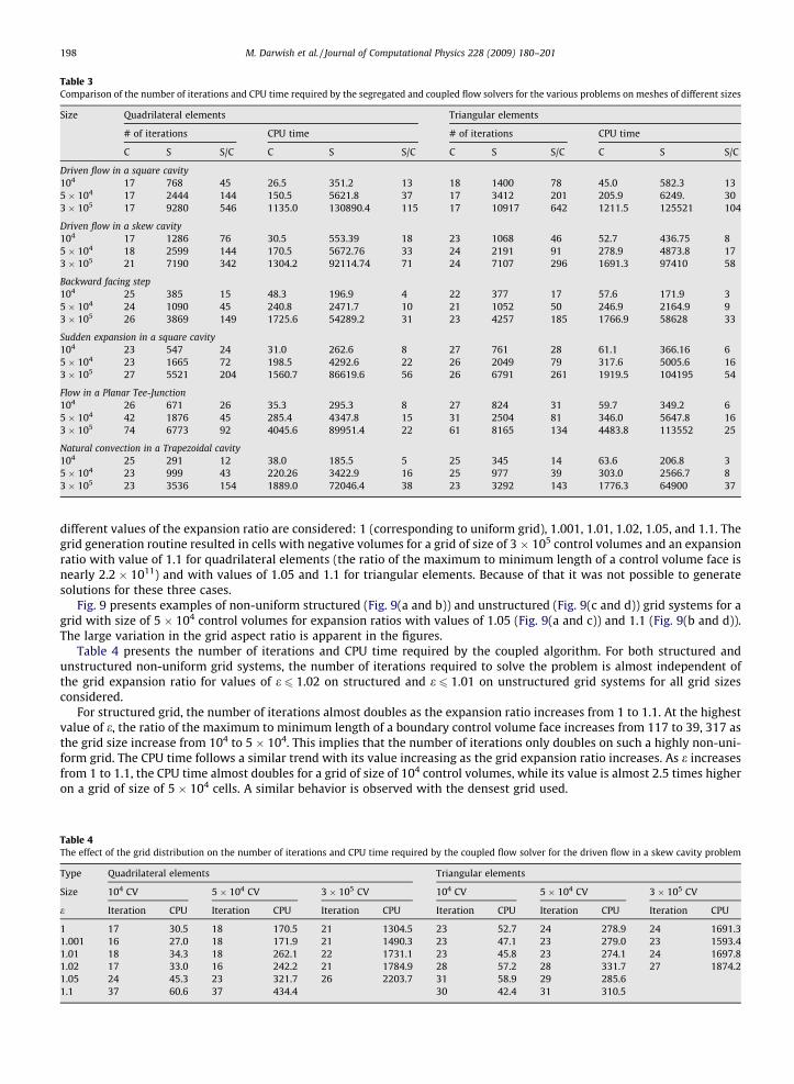
Table 3Comparison of the number of iterations and CPU time required by the segregated and coupled flow solvers for the various problems on meshes of different sizes

Size Quadrilateral elements Triangular elements

# of iterations CPU time # of iterations CPU time

C S S/C C S S/C C S S/C C S S/C

Driven flow in a square cavity104 17 768 45 26.5 351.2 13 18 1400 78 45.0 582.3 135 � 104 17 2444 144 150.5 5621.8 37 17 3412 201 205.9 6249. 303 � 105 17 9280 546 1135.0 130890.4 115 17 10917 642 1211.5 125521 104

Driven flow in a skew cavity104 17 1286 76 30.5 553.39 18 23 1068 46 52.7 436.75 85 � 104 18 2599 144 170.5 5672.76 33 24 2191 91 278.9 4873.8 173 � 105 21 7190 342 1304.2 92114.74 71 24 7107 296 1691.3 97410 58

Backward facing step104 25 385 15 48.3 196.9 4 22 377 17 57.6 171.9 35 � 104 24 1090 45 240.8 2471.7 10 21 1052 50 246.9 2164.9 93 � 105 26 3869 149 1725.6 54289.2 31 23 4257 185 1766.9 58628 33

Sudden expansion in a square cavity104 23 547 24 31.0 262.6 8 27 761 28 61.1 366.16 65 � 104 23 1665 72 198.5 4292.6 22 26 2049 79 317.6 5005.6 163 � 105 27 5521 204 1560.7 86619.6 56 26 6791 261 1919.5 104195 54

Flow in a Planar Tee-Junction104 26 671 26 35.3 295.3 8 27 824 31 59.7 349.2 65 � 104 42 1876 45 285.4 4347.8 15 31 2504 81 346.0 5647.8 163 � 105 74 6773 92 4045.6 89951.4 22 61 8165 134 4483.8 113552 25

Natural convection in a Trapezoidal cavity104 25 291 12 38.0 185.5 5 25 345 14 63.6 206.8 35 � 104 23 999 43 220.26 3422.9 16 25 977 39 303.0 2566.7 83 � 105 23 3536 154 1889.0 72046.4 38 23 3292 143 1776.3 64900 37


different values of the expansion ratio are considered: 1 (corresponding to uniform grid), 1.001, 1.01, 1.02, 1.05, and 1.1. Thegrid generation routine resulted in cells with negative volumes for a grid of size of 3 � 105 control volumes and an expansionratio with value of 1.1 for quadrilateral elements (the ratio of the maximum to minimum length of a control volume face isnearly 2.2 � 1011) and with values of 1.05 and 1.1 for triangular elements. Because of that it was not possible to generatesolutions for these three cases.

Fig. 9 presents examples of non-uniform structured (Fig. 9(a and b)) and unstructured (Fig. 9(c and d)) grid systems for agrid with size of 5 � 104 control volumes for expansion ratios with values of 1.05 (Fig. 9(a and c)) and 1.1 (Fig. 9(b and d)).The large variation in the grid aspect ratio is apparent in the figures.

Table 4 presents the number of iterations and CPU time required by the coupled algorithm. For both structured andunstructured non-uniform grid systems, the number of iterations required to solve the problem is almost independent ofthe grid expansion ratio for values of e 6 1.02 on structured and e 6 1.01 on unstructured grid systems for all grid sizesconsidered.

For structured grid, the number of iterations almost doubles as the expansion ratio increases from 1 to 1.1. At the highestvalue of e, the ratio of the maximum to minimum length of a boundary control volume face increases from 117 to 39, 317 asthe grid size increase from 104 to 5 � 104. This implies that the number of iterations only doubles on such a highly non-uni-form grid. The CPU time follows a similar trend with its value increasing as the grid expansion ratio increases. As e increasesfrom 1 to 1.1, the CPU time almost doubles for a grid of size of 104 control volumes, while its value is almost 2.5 times higheron a grid of size of 5 � 104 cells. A similar behavior is observed with the densest grid used.

Table 4The effect of the grid distribution on the number of iterations and CPU time required by the coupled flow solver for the driven flow in a skew cavity problem

Type Quadrilateral elements Triangular elements

Size 104 CV 5 � 104 CV 3 � 105 CV 104 CV 5 � 104 CV 3 � 105 CV

e Iteration CPU Iteration CPU Iteration CPU Iteration CPU Iteration CPU Iteration CPU

1 17 30.5 18 170.5 21 1304.5 23 52.7 24 278.9 24 1691.31.001 16 27.0 18 171.9 21 1490.3 23 47.1 23 279.0 23 1593.41.01 18 34.3 18 262.1 22 1731.1 23 45.8 23 274.1 24 1697.81.02 17 33.0 16 242.2 21 1784.9 28 57.2 28 331.7 27 1874.21.05 24 45.3 23 321.7 26 2203.7 31 58.9 29 285.61.1 37 60.6 37 434.4 30 42.4 31 310.5

Fig. 9. Non-uniform grid systems with size of 5 � 104 cells for the driven flow in a skew cavity problem using (a and b) quadrilateral and (c and d) triangularelements and expansion ratios of values of (a and c) 1.05 and (b and d) 1.1.


For unstructured grid, the number of iterations varies slightly as the expansion ratio increases, with this number increas-ing from 23 to a maximum of 31 for e = 1.05 (�35% increase in the number of iterations). The variation of CPU time with e isrelatively small with values being slightly dependent on the grid aspect ratio. This difference in performance on structuredand unstructured grids is attributed to the difference in the grid distribution over the computational domain as e increases(compare grid networks in Fig. 9(a–d)).

The decrease, for some cases, in the required CPU time for a given grid size as e increases even though the number of iter-ations required for convergence may be higher is due to the increase in the number of inner iterations needed to satisfy thelocal convergence criteria. For all computations, the residual reduction factor (RRF), defined as the ratio of the root meansquare of the residuals of the algebraic system at the end of an inner iteration to the root mean square of the residuals atthe start of the iteration process is set at 0.01 with the maximum number of iterations of the multigrid solver during anyglobal iteration set at 10. The inner iterative process is stopped when either of the above two conditions is reached, whichexplains the variations in the CPU time.

Finally it should be noted that for structured and unstructured grid systems, the required number of iterations is almostindependent of the grid size at any value of the grid expansion ratio, which is an important characteristic of a coupled solver.

9. Issues and future extensions

Extensions to the above described coupled algorithm could proceed in several directions. In the present work an algebraicmultigrid method was used to accelerate the convergence of the linearized systems of equations. Further improvement toperformance could be achieved by embedding the current algorithm within a Full Multigrid framework (denoted in the lit-erature by the Full Approximation Storage, FAS) whereby inter-equations coupling and non-linearity are dealt with by apply-ing multigrid to the outer iterations [36].

The convective terms have been discretized using the first order upwind scheme [24]. Higher accuracy will be sought byimplementing, within the framework of the normalized variable and space formulation methodology [37], high resolutionschemes following either the deferred correction approach [38] or the more implicit normalized weighting factor method[39].

Two issues that warrant further considerations are turbulence and flow compressibility. With regard to turbulence,appending turbulence models to the system of equations bring additional scalar transport equations (with the numberdepending on the model used) and cause the diffusion coefficients to vary several orders of magnitude within the solution


domain, which is bound to affect the convergence rate. As for flow compressibility, its inclusion will influence the discret-ization of the continuity equation and will require investigating whether to add the energy equation to the coupled system ofcontinuity and momentum equations or to keep it as a separate equation to be solved independently. Both issues will have tobe addressed in future work.

Another matter that deserves attention is the application of the coupled solver to unsteady flows. In most practical sit-uations temporal accuracy can be achieved at a high Courant number. In these cases, multiple iterations of the segregatedsolver are needed for convergence at any one transient step. The performance advantage of the coupled is expected to carryto these situations. However for applications where the time scale necessitates a low courant number, the segregated ap-proach and even the explicit scheme will have an advantage over the coupled approach.

10. Closing remarks

A pressure-based fully coupled method for the solution of laminar incompressible flow problems on unstructured gridwas developed. The method was tested by solving the following five problems: (i) driven flow in a square and a skew cavity,(ii) flow behind a backward facing step, (iii) sudden expansion in a square cavity, (iv) flow in a Planar Tee-Junction, and (v)buoyancy-induced flow in a trapezoidal cavity. The performance of the coupled algorithm was assessed by comparing thenumber of iteration and CPU time required to produce a solution that converged to a desired level with those required usingthe segregated approach. It was found that for problems in which intermediate flow reversals at an outlet boundary do notoccur during the solution, the number of iterations needed by the coupled algorithm is grid independent. Moreover, resultsshowed a substantial decrease in computational time using the coupled approach when compared to using the segregatedmethod with the reduction rate increasing as the grid size increases. The CPU times required by the coupled solver on struc-tured and unstructured grids depended on the grid size with the time required on relatively coarse structured meshes beinglower. Low and moderate variation in the grid aspect ratio did not alter the required number of outer iterations but, rather,affected the time consumed by the inner iterations with the CPU time increasing as the grid expansion ratio increases. At anygrid expansion ratio, the required number of iterations was almost independent of the grid size.

Acknowledgments

The financial support provided by the University Research Board of the American University of Beirut through Grant #888322 is gratefully acknowledged.

References

[1] F. Moukalled, M. Darwish, A high resolution pressure-based algorithm for fluid flow at all speeds, Journal of Computational Physics 169 (1) (2001) 101–133.

[2] W. Rodi, S. Majumdar, B. Schonung, Finite volume methods for two-dimensional incompressible flows with complex boundaries, Computer Methods inApplied Mechanics and Engineering 75 (1989) 369–392.

[3] F. Moukalled, M. Darwish, Pressure-based algorithms for single-fluid and multifluid flows, in: W.J. Minkowycz, E.M. Sparrow, J.Y. Murthy (Eds.),Handbook of Numerical Heat Transfer, second ed., Wiley, 2006, pp. 325–367.

[4] G.B. Deng, J. Piquet, X. Vasseur, M. Visonneau, A new fully coupled method for computing turbulent flows, Computers and Fluids 30 (2001) 445–472.[5] R. Webster, An algebraic multigrid solver for Navier–Stokes problems, International Journal for Numerical Methods in Fluids 18 (1994) 761–780.[6] R.F. Hanby, D.J. Silvester, A comparison of coupled and segregated iterative solution techniques for incompressible swirling flow, International Journal

for Numerical Methods in Fluids 22 (1996) 353–373.[7] F.H. Harlow, J.E. Welch, Numerical calculation of time-dependent viscous incompressible flow of fluid with free surface, Physics of Fluids 8 (1965)

2182–2189.[8] A.J. Chorin, Numerical solution of the Navier–Stokes equation, Mathematics of Computation 22 (1971) 745–762.[9] S.V. Patankar, D.B. Spadling, A calculation procedure for heat, mass and momentum transfer in three-dimensional parabolic flows, International Journal

of Heat and Mass Transfer 15 (1972) 1787–1806.[10] F. Moukalled, M. Darwish, A unified formulation of the segregated class of algorithms for fluid flow at all speeds, Numerical Heat Transfer, Part B 37 (1)

(2000) 103–139.[11] C.M. Rhie, W.L. Chow, A numerical study of the turbulent flow past an isolated airfoil with trailing edge separation, AIAA Journal 21 (1983) 1525–1532.[12] G.E. Schneider, G.D. Raithby, M.M. Yonavovich, Finite element analysis of incompressible fluid flow incorporating equal order pressure and velocity

interpolation, in: C. Taylor, K. Morgan, C.A. Brebbia (Eds.), Numerical Methods in Laminar and Turbulent Flow, Pentech Press, London, 1978.[13] P. Brufau, P. Garcı́a-Navarro, Unsteady free surface flow simulation over complex topography with a multidimensional upwind technique, Journal of

Computational Physics 186 (2) (2003) 503–526.[14] M. Darwish, F. Moukalled, B. Sekar, A unified formulation of the segregated class of algorithms for multi-fluid flow at all speeds, Numerical Heat

Transfer, Part B 40 (2) (2001) 99–137.[15] F. Moukalled, M. Darwish, B. Sekar, A high resolution pressure-based algorithm for multi-phase flow at all speeds, Journal of Computational Physics

190 (2003) 550–571.[16] L.S. Caretto, R.M. Curr, D.B. Spalding, Two numerical methods for three-dimensional boundary layers, Computer Methods in Applied Mechanics and

Engineering 1 (1972) 39–57.[17] S.P. Vanka, Block-implicit multigrid solution of Navier–Stokes equations in primitive variables, Journal of Computational Physics 65 (1) (1986) 138–

158.[18] K.C. Karki, H.C. Mongia, Evaluation of a coupled solution approach for fluid flow calculations in body fitted co-ordinates, International Journal for

Numerical Methods in Fluids 11 (1990) 1–20.[19] Braaten, M.E., Development and evaluation of iterative and direct methods for the solution of the equations governing recirculating flows, Ph.D. Thesis,

University of Minnesota, May 1985.[20] Z. Mazhar, A procedure for the treatment of the velocity-pressure coupling problem in incompressible fluid flow, Numerical Heat Transfer, Part B 39

(2001) 91–100.


[21] A. Pascau, C. Pérez, F.J. Serón, A comparison of segregated and coupled methods for the solution of the incompressible Navier–Stokes equations,Communications in Numerical Methods in Engineering 12 (1996) 617–630.

[22] P.F. Galpin, G.D. Raithby, Numerical solution of problems in incompressible fluid flow: treatment of the temperature-velocity coupling, Numerical HeatTransfer 10 (1986) 105–129.

[23] I. Ammara, C. Masson, Development of a fully coupled control-volume finite element method for the incompressible Navier–Stokes equations,International Journal for Numerical Methods in Fluids 44 (2004) 621–644.

[24] S.V. Patankar, Numerical Heat Transfer and Fluid Flow, Hemisphere, NY, 1981.[25] Van Doormal, J.P., Numerical methods for the solution of incompressible and compressible fluid flows, PhD Thesis, University of Waterloo, Ontario,

Canada, 1985.[26] R.D. Lonsdale, An algebraic multigrid scheme for solving the Navier–Stokes equations on unstructured meshes, in: C. Taylor, J.H. Chin, G.M. Homsy

(Eds.), Numerical Methods in Laminar and Turbulent Flow, vol. 7, Pineridge Press, Swansea, UK, 1991, pp. 1432–1442. part 2.[27] M. Darwish, I. Sraj, F. Moukalled, A coupled incompressible flow solver on structured grids, Numerical Heat Transfer, Part B 52 (2007) 353–371.[28] C. Pommerell, W. Fichtner, Memory aspects and performance of iterative solvers, SIAM Journal of Scientific and Statistical Computing 15 (1994) 460–

473.[29] B.R. Hutchinson, G.D. Raithby, A multigrid method based on the additive correction strategy, Numerical Heat Transfer 9 (1986) 511–537.[30] R.P. Fedorenko, A relaxation method for solving elliptic difference equations, USSR Computational Mathematics and Mathematical Physics 1 (1962)

1092–1096.[31] F.V. Poussin, An accelerated relaxation algorithm for iterative solution of elliptic equations, SIAM Journal of Numerical Analysis 5 (1968) 340–351.[32] A. Brandt, Multi-level adaptive solutions to boundary value problems, Mathematics of Computations 31 (138) (1977) 333–390.[33] S.R. Elias, G.D. Stubley, G.D. Raithby, An adaptive agglomeration method for additive correction multigrid, International Journal for Numerical Methods

in Engineering 40 (1997) 887–903.[34] R.E. Hayes, K. Nandakumar, H. Nasr-El-Din, Steady laminar flow in a 90 degree planar branch, Computers and Fluids 17 (1989) 537–553.[35] F. Moukalled, M. Darwish, Natural Convection in a Partitioned Trapezoidal Cavity Heated from the Side, Numerical Heat Transfer, Part A 43 (5) (2003)

543–563.[36] M. Darwish, F. Moukalled, B. Sekar, A Robust multi-grid algorithm for multifluid flow at all speeds, International Journal for Numerical Methods in

Fluids 41 (2003) 1221–1251.[37] M. Darwish, F. Moukalled, Normalized variable and space formulation methodology for high-resolution schemes, Numerical Heat Transfer, Part B 26

(1) (1994) 79–96.[38] S.G. Rubin, P.K. Khosla, Polynomial interpolation method for viscous flow calculations, Journal of Computational Physics 27 (1982) 153–168.[39] M. Darwish, F. Moukalled, The normalized weighting factor method: a novel technique for accelerating the convergence of high-resolution convective

schemes, Numerical Heat Transfer, Part B 30 (2) (1996) 217–237.

A coupled finite volume solver for the solution of ...

Documents

Transcript of A coupled finite volume solver for the solution of ...