Journal of Applied Fluid Mechanics, Vol. 7, No. 4, pp. 673-682, 2014.

Available online at www.jafmonline.net, ISSN 1735-3572, EISSN 1735-3645.

Development of a Segregated Compressible Flow Solver

for Turbomachinery Simulations

J. Benajes1, J. Galindo

1, P. Fajardo

2 and R. Navarro

1†

1 CMT - Motores Térmicos, Universitat Politècnica de València, Camino de Vera S/N, Valencia, 46022,

Spain 2 Bioingeniería e Ingeniería Aeroespacial, Universidad Carlos III de Madrid, Leganés, 28911, Spain

†Corresponding Author Email: ronagar1@mot.upv.es

(Received September 10, 2013; accepted January 13, 2014)

ABSTRACT

A steady multiple reference frame segregated compressible solver and an unsteady sliding mesh one are

developed using OpenFOAM® to simulate turbomachinery. For each of the two solvers, governing

equations, numerical approach and solver structure are explained. Pressure and energy equation are

implemented so as to obtain the best numerical properties, such as the ability to use large time-steps. Sod

shock tube test case is used to assess the prediction of compressible phenomena by the transient scheme,

which shows proper resolution of compressible waves. Both solvers are used to simulate a turbocharger

turbine, comparing their solutions to corresponding ones using ANSYS® Fluent® as a means of validation.

The multiple reference frame solver global results quantitatively differ from those computed using ANSYS

Fluent, although predicted flow features match. The solution obtained by the sliding mesh solver presents

better agreement compared to ANSYS Fluent one.

Keywords: CFD, OpenFOAM, Multiple Reference Frame, Sliding Mesh.

NOMENCLATURE

Symbols

d A differential area vector (m2) u

pa diagonal coefficients of momentum

equation (kg · m-3 · s-1)

pc specific heat capacity at constant

pressure (J · kg-1 · K-1)

h specific enthalpy (m2 · s-2)

H v off-diagonal part of the momentum

equation matrix and source terms

excluding pressure gradient (kg · m-2 · s-2)

k turbulent kinetic energy (m2 · s-2)

p pressure (Pa)

r position vector (m)

R specific gas constant (J · kg-1 · K-1)

t time (s)

T temperature (K)

v velocity (m · s-1)

isentropic efficiency

specific heats ratio

thermal conductivity (kg · m · s-3 · K-1)

pressure ratio

d pseudo-flux (m-1 · s)

compressibility (m-2 · s2)

density (kg · m-3)

viscous stress tensor (Pa)

rotational speed (rad · s-1)

Sub- and Superscripts

0 stagnation variable

eff effective value

in inlet value

f values at faces of control volumes

out outlet value

p value for generic point P

r relative

ref reference value

Abbreviations

BC boundary condition

CFD computational fluid dynamics

EOS equation of state

GGI general grid interface

MRF multiple reference frame

SM sliding mesh

URF under-relaxation factor

J. Benajes et al. / JAFM, Vol. 7, No. 4, pp. 673-682, 2014.

674

1. INTRODUCTION

CFD has become an essential tool in

turbomachinery design and analysis, particularly in

automotive turbochargers. The flow passing

through this type of radial turbomachinery must be

considered as compressible, due to the high Mach

numbers (Simpson et al. 2009). When simulating

compressible flow, there are two types of solvers.

The so-called density based solvers can be

employed, in which the use of Riemann solvers

enhances the ability to capture shocks (Toro 1999).

These solvers are thus well-suited for solving

hypersonic flow problems (Nair et al. 2010).

However, they have a high computational cost, over

all when dealing with steady computations, since

they rely on a time-marching process. Computation

of subsonic/transonic turbomachinery flows can

also be carried out by pressure-based segregated

solvers, in which a pressure equation is derived

from continuity and momentum equations. Since

the governing equations are resolved in a sequential

fashion, a pressure-velocity coupling method is

required, such as the well known SIMPLE

(Patankar and Spalding 1972) or PISO (Issa 1986)

algorithms.

Another important feature in solvers used to

simulate turbomachinery is the strategy to deal with

rotor motion. There are two main methods. On the

one side, there is the Multiple Reference Frame

(MRF) approach, also known as frozen rotor, in

which the mesh does not move and the impeller

region is modeled with a rotating frame. This

technique allows solving a set of steady equations,

thus having little computational cost. Several

authors have studied the accuracy of this method

(Hillewaert and Van den Braembussche 1999; Liu

and Hill 2000; Zheng et al. 2010). The general

agreement is that MRF is not the most appropriate

approach for radial turbomachinery simulations,

especially when predicting flow features at off-

design conditions. However, due to its low

computational cost, it is useful as a first hint of the

turbomachinery performance or as a means of

initialization for more complex methods. On the

other side, the Sliding Mesh (SM) approach

considers the unsteady equations, rotating the

impeller mesh at every time-step.

Reaching a periodic state requires 10 to 100 times

more computational cost than obtaining the

converged steady solution with MRF. However,

transient features are resolved, which is of

importance when simulating turbomachinery at off-

design operating conditions (Galindo et al. 2013a).

The SM method has been proved to give good

results (Hellstrom 2010; Guo et al. 2007; Chen et

al. 2008).

One of the codes whose use is steadily increasing is

OpenFOAM. OpenFOAM (OpenCFD Ltd 2004-

2013) is an open source toolbox for the solution of

continuum mechanics problems. OpenFOAM has

been used for several incompressible

turbomachinery simulations. Auvinen et al. (2009)

conducted a numerical study of a single-channel

pump, comparing CFD results against experimental

data. Transient simulation were performed using a

sliding mesh approach with the aid of a General

Grid Interface (GGI), a tool developed by Beaudoin

and Jasak (2008). The effect of mesh density,

turbulence models, time-step, and length of inlet

duct on overall parameters such as hydrodynamic

head, shaft power or efficiency was checked.

Moreover, velocity profiles predicted by the

different numerical configurations are compared

with Laser Doppler Velocimetry measurements.

Petit et al. (2009) compared frozen rotor and sliding

grid 2D simulations of the ERCOFTAC centrifugal

pump against experimental data obtained by Ubaldi

et al. (1996). GGI variants and additional

turbomachinery simulations performed with

OpenFOAM can be found in Jasak (2011).

Regarding compressible flow turbomachinery

simulations using OpenFOAM, Borm et al.

(2011a,b; 2012) developed and tested several

density-based solvers with MRF and SM

capabilities, which are available at one branch of

the Extend Project Borm (2012). Mangani et al.

(2007) developed a pressure-based segregated

compressible solver in OpenFOAM, using a

pressure corrector equation. However, rotor motion

methods were not discussed. Mangani et al. (2012)

investigated the effect of turbulence models on the

prediction of centrifugal compressor global

variables and local flow field. Gröschel et al. (2012)

used an improved version of this solver with a MRF

approach to optimize a high pressure ratio

centrifugal compressor, although the

implementation of the MRF method is not

described.

The main advantages of OpenFOAM are that it is

free of charge, so it does not have any license code

nor license manager problems, and it is an open

code, which allows one to modify almost every

single detail of it. However, since the code is

relatively young, it lacks some capabilities and

some existing ones have not been thoroughly

validated. For instance, there are no compressible

pressure based solvers available in OpenFoam

having a built-in rotor motion capability, which is a

must in turbomachinery applications, and allowing

to perform computations with large time-step size.

The objective of this paper is therefore to develop

compressible pressure-based segregated solvers for

turbomachinery flow simulations using

OpenFOAM, with both MRF and SM approaches.

The solvers have been implemented in

OpenFOAM-1.6-ext.

For each of the two solvers, corresponding

governing equations will be first presented and the

solver structure will be explained. Then, the solver

will be used to simulate a turbocharger turbine,

comparing the solution obtained to the one

computed using ANSYS Fluent.

2. MULTIPLE REFERENCE

FRAME

The governing equations in a rotating reference

frame, using the absolute velocity formulation, can

be expressed as:

J. Benajes et al. / JAFM, Vol. 7, No. 4, pp. 673-682, 2014.

675

0

( ) 0

( ) ( )

( ) ( )

r

r

r eff

v

v v v p

v h p r T v

p RT

(1)

where total enthalpy is defined as:

2

0

| |

2

vh h k . (2)

The differences between Eq. (1) and the ordinary

Navier-Stokes equations are that the advective

terms are computed with a relative flux

rv v r and there are new terms due to non

inertial effects.

It is important to highlight that energy equation has

been considered using total enthalpy because it

provides a conservative formulation. Since a

segregated approach is sought, the pressure

equation is derived using continuity and momentum

ones following the work by Jasak (2006), resulting

in Eq. (3): 1

, ( ( ) )u

d f f p

f

p a p . (3)

Left hand side of Eq. (3) has been integrated over a

control volume using a linearized and discretized

form of Gauss’ theorem. Since Eq. (3) is not a

pressure corrector equation, implicit under-

relaxation can be performed, thus improving the

linear solver stability (Ferziger and Peric 2002), and

the restrictions on boundary conditions described by

Mangani (2008) are not present. In Eq. (3) a

pseudo-flux, d , is used as presented by Jasak

(1996). d is computed as shown in Eq. (4):

1( ) ( ) ,u

d pa H v dA (5)

in which the pseudo-velocity employed, 1( ) ( )u

pa H v , does not carry the pressure gradient

contribution. The pseudo-velocity field can be

obtained rearrainging the momentum equation, as

shown in Eq. (6):

( )u

p pa v H v p , (6)

where the terms of the equation have been separated

in the diagonal terms, u

p pa v , and the off-diagonal

part and rest of the sources of the equation

excluding the pressure gradient, represented by the

operator ( )H v . Additionally, since it is a MRF

solver, the flux in the rotating domain has to be

relative to the rotating reference frame, as:

1

, ( ) ( )u

d r pa H v r dA .

(7)

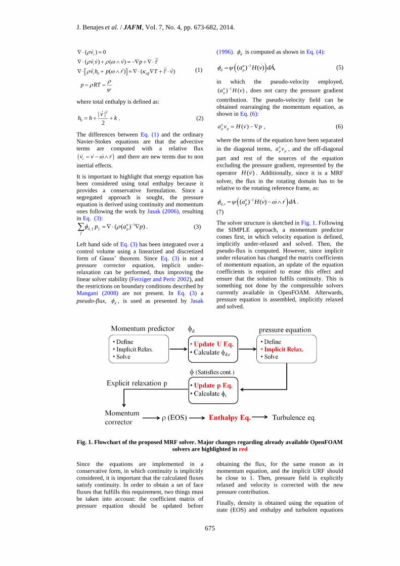
The solver structure is sketched in Fig. 1. Following

the SIMPLE approach, a momentum predictor

comes first, in which velocity equation is defined,

implicitly under-relaxed and solved. Then, the

pseudo-flux is computed. However, since implicit

under relaxation has changed the matrix coefficients

of momentum equation, an update of the equation

coefficients is required to erase this effect and

ensure that the solution fulfils continuity. This is

something not done by the compressible solvers

currently available in OpenFOAM. Afterwards,

pressure equation is assembled, implicitly relaxed

and solved.

Fig. 1. Flowchart of the proposed MRF solver. Major changes regarding already available OpenFOAM

solvers are highlighted in red

Since the equations are implemented in a

conservative form, in which continuity is implicitly

considered, it is important that the calculated fluxes

satisfy continuity. In order to obtain a set of face

fluxes that fulfills this requirement, two things must

be taken into account: the coefficient matrix of

pressure equation should be updated before

obtaining the flux, for the same reason as in

momentum equation, and the implicit URF should

be close to 1. Then, pressure field is explicitly

relaxed and velocity is corrected with the new

pressure contribution.

Finally, density is obtained using the equation of

state (EOS) and enthalpy and turbulent equations

J. Benajes et al. / JAFM, Vol. 7, No. 4, pp. 673-682, 2014.

676

are solved. After that, a new iteration is performed.

Regarding enthalpy equation, it has been placed

after the pressure-velocity coupling to have a

consistent set of pressure and velocity fields and

fluxes when solving it. If the fluid cell considered

belongs to the rotor, the corresponding non-inertial

terms must be added prior to solving momentum

and energy equations and the fluxes should be made

relative to the rotating reference frame after its

computation.

The developed solver was used to simulate the

variable geometry turbine analyzed by Galindo et

al. (2013b) under different operating conditions,

providing good convergence behavior. The solution

obtained by this solver is compared to the one

computed using ANSYS Fluent. The same setup,

described in Table 1, is used in both codes. First

order discretization schemes have been chosen for

the current simulations. This selection is based on

the fact that the implementation of 1st order

schemes is unequivocal while the implementation

of a 2nd order scheme could have different

approaches in each code, and the goal of the

simulations is not accuracy of the solution but

comparability across codes.

Table 1 MRF configuration parameters

Discretization

schemes 1st order

Inlet BC

Mass flow (0.065, 0.075,

0.085, 0.095 kg/s),

total temperature (664 K)

Outlet BC Static pressure (101325 Pa)

Wall heat transfer

model Adiabatic

Turbulence model RNG k-ε

Rotational speed 18953 rad/s

Thermal properties

(cp, κ, etc.)

Constant values for dry air at

664 K

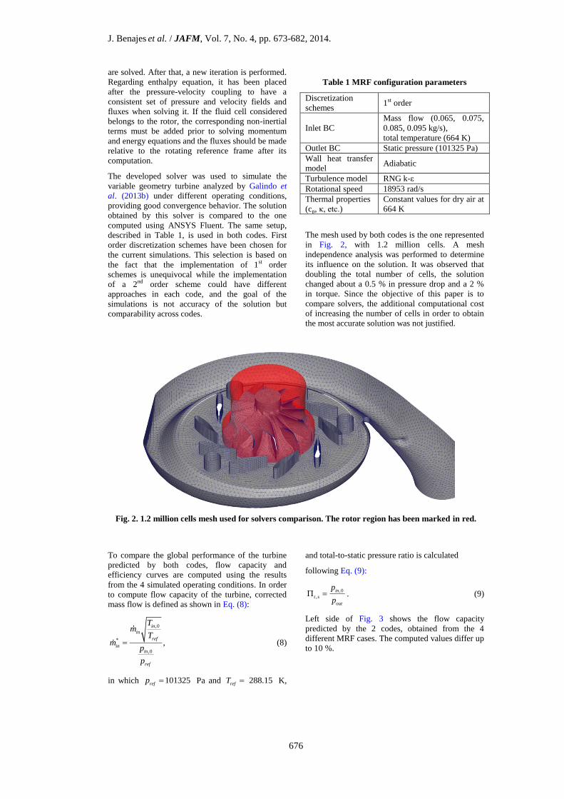
The mesh used by both codes is the one represented

in Fig. 2, with 1.2 million cells. A mesh

independence analysis was performed to determine

its influence on the solution. It was observed that

doubling the total number of cells, the solution

changed about a 0.5 % in pressure drop and a 2 %

in torque. Since the objective of this paper is to

compare solvers, the additional computational cost

of increasing the number of cells in order to obtain

the most accurate solution was not justified.

Fig. 2. 1.2 million cells mesh used for solvers comparison. The rotor region has been marked in red.

To compare the global performance of the turbine

predicted by both codes, flow capacity and

efficiency curves are computed using the results

from the 4 simulated operating conditions. In order

to compute flow capacity of the turbine, corrected

mass flow is defined as shown in Eq. (8):

,0

*

,0

,

in

in

ref

inin

ref

Tm

Tm

p

p

(8)

in which 101325refp Pa and 288.15refT K,

and total-to-static pressure ratio is calculated

following Eq. (9):

,0

,

in

t s

out

p

p . (9)

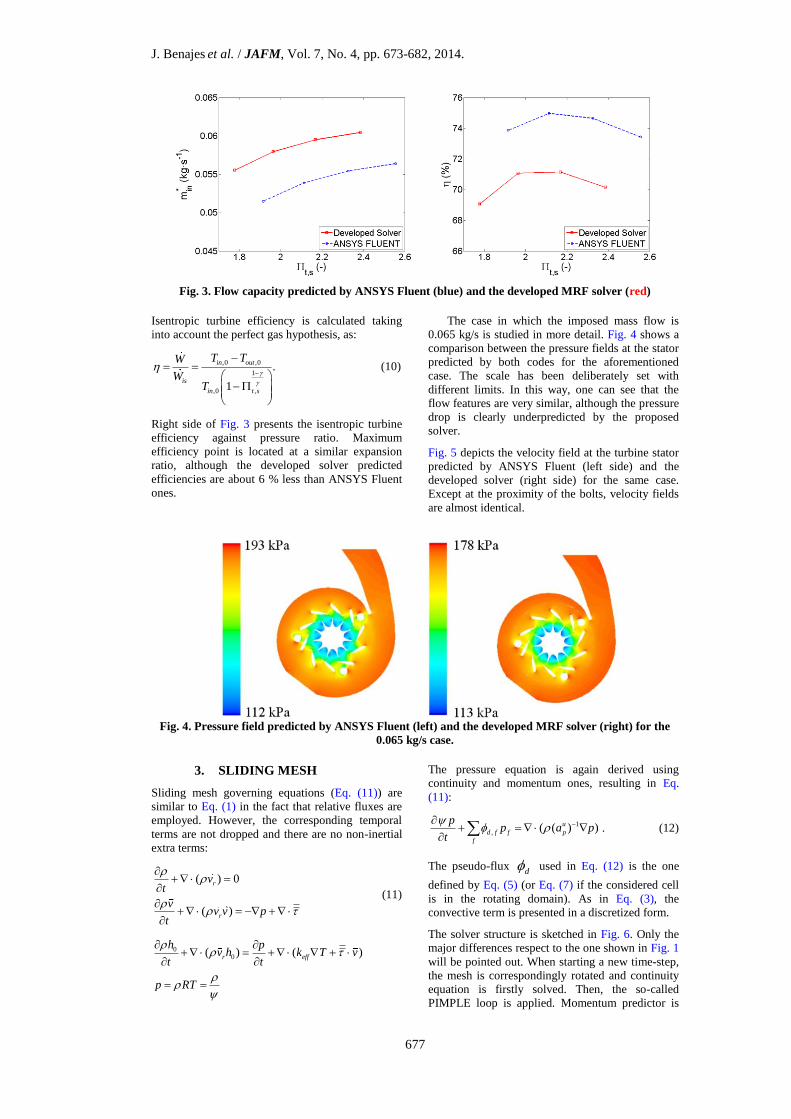
Left side of Fig. 3 shows the flow capacity

predicted by the 2 codes, obtained from the 4

different MRF cases. The computed values differ up

to 10 %.

J. Benajes et al. / JAFM, Vol. 7, No. 4, pp. 673-682, 2014.

677

Fig. 3. Flow capacity predicted by ANSYS Fluent (blue) and the developed MRF solver (red)

Isentropic turbine efficiency is calculated taking

into account the perfect gas hypothesis, as:

,0 ,0

1

,0 ,

.

1

in out

is

in t s

T TW

WT

(10)

Right side of Fig. 3 presents the isentropic turbine

efficiency against pressure ratio. Maximum

efficiency point is located at a similar expansion

ratio, although the developed solver predicted

efficiencies are about 6 % less than ANSYS Fluent

ones.

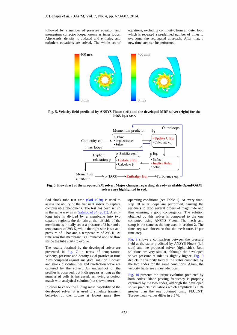
The case in which the imposed mass flow is

0.065 kg/s is studied in more detail. Fig. 4 shows a

comparison between the pressure fields at the stator

predicted by both codes for the aforementioned

case. The scale has been deliberately set with

different limits. In this way, one can see that the

flow features are very similar, although the pressure

drop is clearly underpredicted by the proposed

solver.

Fig. 5 depicts the velocity field at the turbine stator

predicted by ANSYS Fluent (left side) and the

developed solver (right side) for the same case.

Except at the proximity of the bolts, velocity fields

are almost identical.

Fig. 4. Pressure field predicted by ANSYS Fluent (left) and the developed MRF solver (right) for the

0.065 kg/s case.

3. SLIDING MESH

Sliding mesh governing equations (Eq. (11)) are

similar to Eq. (1) in the fact that relative fluxes are

employed. However, the corresponding temporal

terms are not dropped and there are no non-inertial

extra terms:

( ) 0

( )

r

r

vt

vv v p

t

(11)

00 )( ( )r eff

h pv h k T v

t t

p RT

The pressure equation is again derived using

continuity and momentum ones, resulting in Eq.

(11):

1

, ( ( ) )u

d f f p

f

pp a p

t

. (12)

The pseudo-flux d used in Eq. (12) is the one

defined by Eq. (5) (or Eq. (7) if the considered cell

is in the rotating domain). As in Eq. (3), the

convective term is presented in a discretized form.

The solver structure is sketched in Fig. 6. Only the

major differences respect to the one shown in Fig. 1

will be pointed out. When starting a new time-step,

the mesh is correspondingly rotated and continuity

equation is firstly solved. Then, the so-called

PIMPLE loop is applied. Momentum predictor is

J. Benajes et al. / JAFM, Vol. 7, No. 4, pp. 673-682, 2014.

678

followed by a number of pressure equation and

momentum corrector loops, known as inner loops.

Afterwards, density is updated and enthalpy and

turbulent equations are solved. The whole set of

equations, excluding continuity, form an outer loop

which is repeated a predefined number of times to

overcome the segregated approach. After that, a

new time-step can be performed.

Fig. 5. Velocity field predicted by ANSYS Fluent (left) and the developed MRF solver (right) for the

0.065 kg/s case.

Fig. 6. Flowchart of the proposed SM solver. Major changes regarding already available OpenFOAM

solvers are highlighted in red.

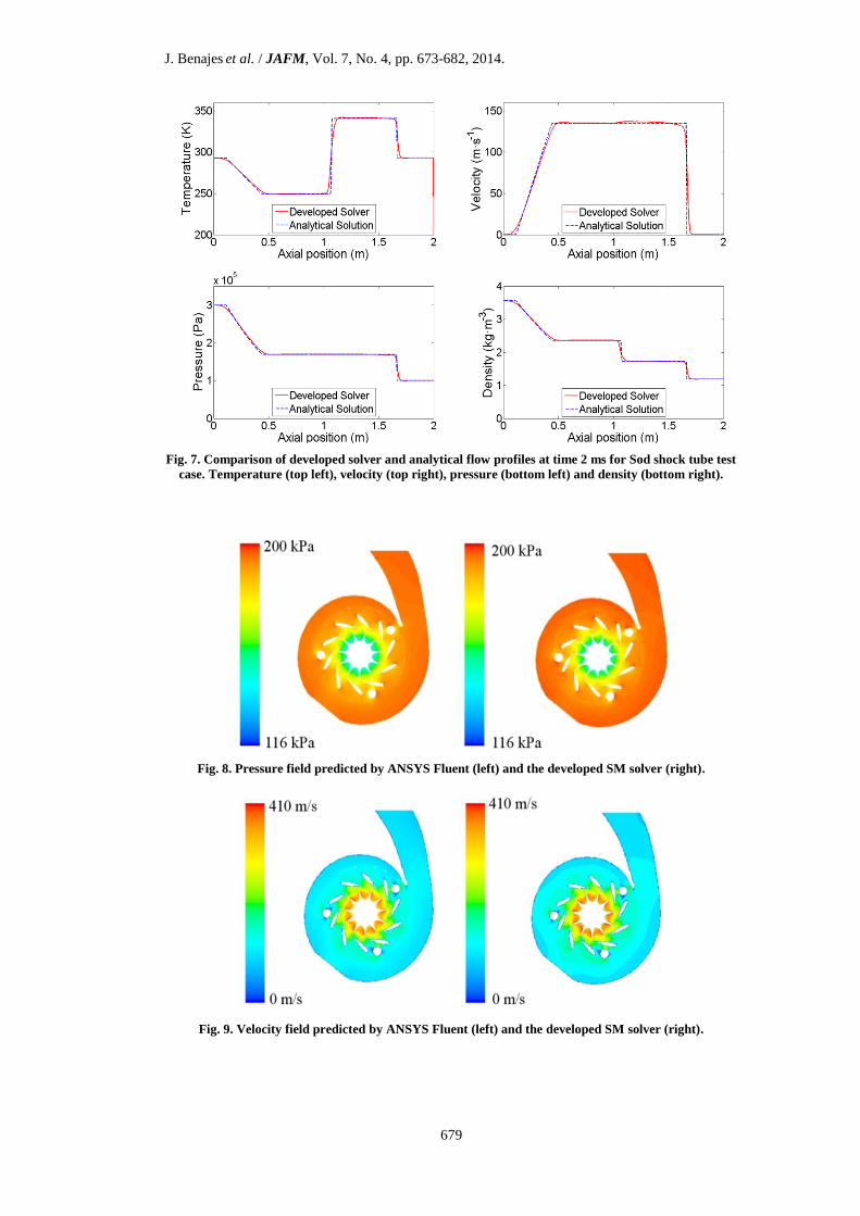
Sod shock tube test case (Sod 1978) is used to

assess the ability of the transient solver to capture

compressible phenomena. The test has been set up

in the same way as in Galindo et al. (2011). A 2-m-

long tube is divided by a membrane into two

separate regions: the domain at the left side of the

membrane is initially set at a pressure of 3 bar and a

temperature of 293 K, while the right side is set at a

pressure of 1 bar and a temperature of 293 K. At

time zero this membrane is eliminated and the flow

inside the tube starts to evolve.

The results obtained by the developed solver are

presented in Fig. 7 in terms of temperature,

velocity, pressure and density axial profiles at time

2 ms compared against analytical solution. Contact

and shock discontinuities and rarefaction wave are

captured by the solver. An undershoot of the

profiles is observed, but it disappears as long as the

number of cells is increased, achieving a perfect

match with analytical solution (not shown here).

In order to check the sliding mesh capability of the

developed solver, it is used to simulate transient

behavior of the turbine at lowest mass flow

operating conditions (see Table 1). At every time-

step 10 outer loops are performed, causing the

residuals to drop several orders of magnitude and

thus ensuring a good convergence. The solution

obtained by this solver is compared to the one

computed using ANSYS Fluent. The mesh and

setup is the same as the one used in section 2. The

time-step was chosen so that the mesh turns 1º per

time-step.

Fig. 8 shows a comparison between the pressure

field at the stator predicted by ANSYS Fluent (left

side) and the proposed solver (right side). Both

solutions are very similar, although the developed

solver pressure at inlet is slightly higher. Fig. 9

depicts the velocity field at the stator computed by

the two codes for the same conditions. Again, the

velocity fields are almost identical.

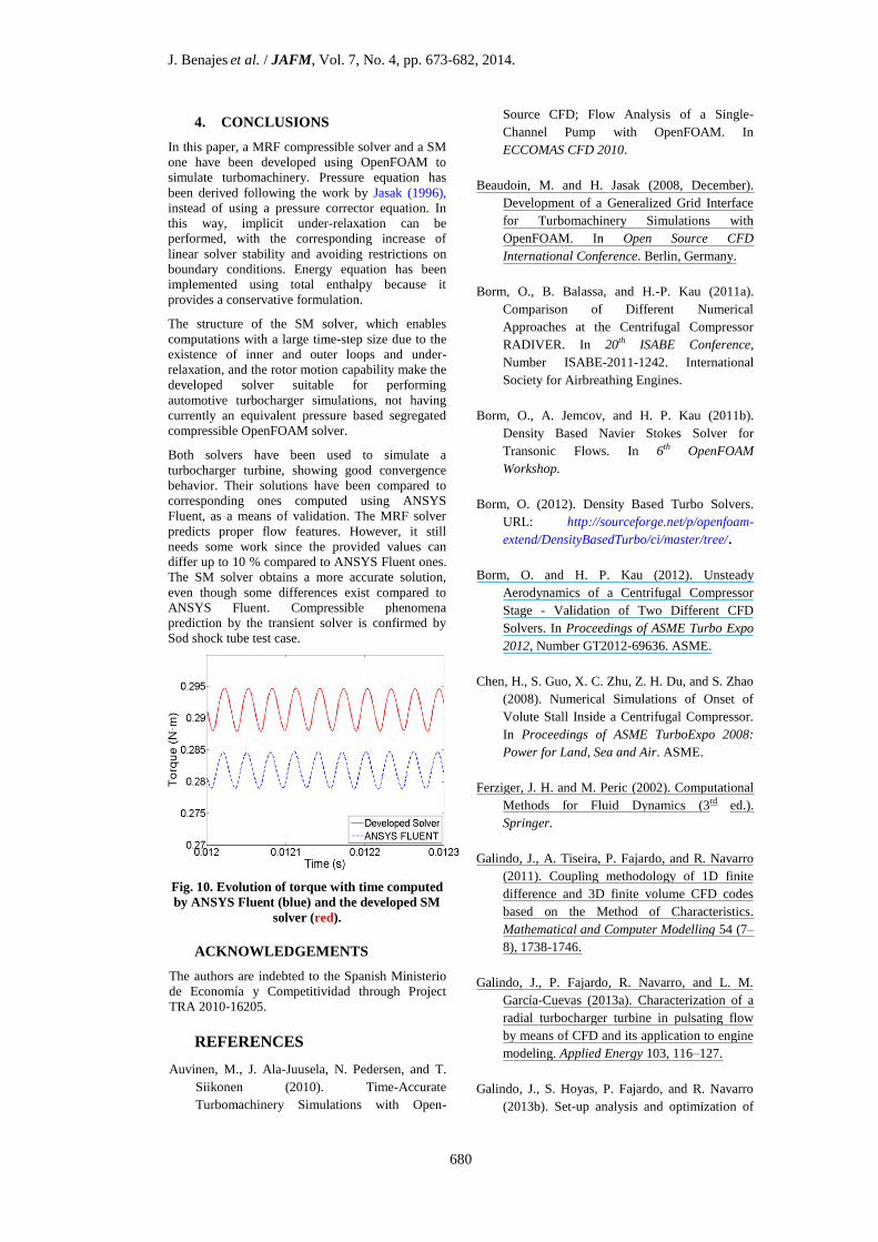
Fig. 10 presents the torque evolution predicted by

both codes. Blade passing frequency is properly

captured by the two codes, although the developed

solver predicts oscillations which amplitude is 15%

greater than the one obtained using FLUENT.

Torque mean values differ in 3.5 %.

J. Benajes et al. / JAFM, Vol. 7, No. 4, pp. 673-682, 2014.

679

Fig. 7. Comparison of developed solver and analytical flow profiles at time 2 ms for Sod shock tube test

case. Temperature (top left), velocity (top right), pressure (bottom left) and density (bottom right).

Fig. 8. Pressure field predicted by ANSYS Fluent (left) and the developed SM solver (right).

Fig. 9. Velocity field predicted by ANSYS Fluent (left) and the developed SM solver (right).

J. Benajes et al. / JAFM, Vol. 7, No. 4, pp. 673-682, 2014.

680

4. CONCLUSIONS

In this paper, a MRF compressible solver and a SM

one have been developed using OpenFOAM to

simulate turbomachinery. Pressure equation has

been derived following the work by Jasak (1996),

instead of using a pressure corrector equation. In

this way, implicit under-relaxation can be

performed, with the corresponding increase of

linear solver stability and avoiding restrictions on

boundary conditions. Energy equation has been

implemented using total enthalpy because it

provides a conservative formulation.

The structure of the SM solver, which enables

computations with a large time-step size due to the

existence of inner and outer loops and under-

relaxation, and the rotor motion capability make the

developed solver suitable for performing

automotive turbocharger simulations, not having

currently an equivalent pressure based segregated

compressible OpenFOAM solver.

Both solvers have been used to simulate a

turbocharger turbine, showing good convergence

behavior. Their solutions have been compared to

corresponding ones computed using ANSYS

Fluent, as a means of validation. The MRF solver

predicts proper flow features. However, it still

needs some work since the provided values can

differ up to 10 % compared to ANSYS Fluent ones.

The SM solver obtains a more accurate solution,

even though some differences exist compared to

ANSYS Fluent. Compressible phenomena

prediction by the transient solver is confirmed by

Sod shock tube test case.

Fig. 10. Evolution of torque with time computed

by ANSYS Fluent (blue) and the developed SM

solver (red).

ACKNOWLEDGEMENTS

The authors are indebted to the Spanish Ministerio

de Economía y Competitividad through Project

TRA 2010-16205.

REFERENCES

Auvinen, M., J. Ala-Juusela, N. Pedersen, and T.

Siikonen (2010). Time-Accurate

Turbomachinery Simulations with Open-

Source CFD; Flow Analysis of a Single-

Channel Pump with OpenFOAM. In

ECCOMAS CFD 2010.

Beaudoin, M. and H. Jasak (2008, December).

Development of a Generalized Grid Interface

for Turbomachinery Simulations with

OpenFOAM. In Open Source CFD

International Conference. Berlin, Germany.

Borm, O., B. Balassa, and H.-P. Kau (2011a).

Comparison of Different Numerical

Approaches at the Centrifugal Compressor

RADIVER. In 20th ISABE Conference,

Number ISABE-2011-1242. International

Society for Airbreathing Engines.

Borm, O., A. Jemcov, and H. P. Kau (2011b).

Density Based Navier Stokes Solver for

Transonic Flows. In 6th OpenFOAM

Workshop.

Borm, O. (2012). Density Based Turbo Solvers.

URL: http://sourceforge.net/p/openfoam-

extend/DensityBasedTurbo/ci/master/tree/.

Borm, O. and H. P. Kau (2012). Unsteady

Aerodynamics of a Centrifugal Compressor

Stage - Validation of Two Different CFD

Solvers. In Proceedings of ASME Turbo Expo

2012, Number GT2012-69636. ASME.

Chen, H., S. Guo, X. C. Zhu, Z. H. Du, and S. Zhao

(2008). Numerical Simulations of Onset of

Volute Stall Inside a Centrifugal Compressor.

In Proceedings of ASME TurboExpo 2008:

Power for Land, Sea and Air. ASME.

Ferziger, J. H. and M. Peric (2002). Computational

Methods for Fluid Dynamics (3rd ed.).

Springer.

Galindo, J., A. Tiseira, P. Fajardo, and R. Navarro

(2011). Coupling methodology of 1D finite

difference and 3D finite volume CFD codes

based on the Method of Characteristics.

Mathematical and Computer Modelling 54 (7–

8), 1738-1746.

Galindo, J., P. Fajardo, R. Navarro, and L. M.

García-Cuevas (2013a). Characterization of a

radial turbocharger turbine in pulsating flow

by means of CFD and its application to engine

modeling. Applied Energy 103, 116–127.

Galindo, J., S. Hoyas, P. Fajardo, and R. Navarro

(2013b). Set-up analysis and optimization of

J. Benajes et al. / JAFM, Vol. 7, No. 4, pp. 673-682, 2014.

681

CFD simulations for radial turbines.

Engineering Applications of Computational

Fluid Mechanics 7(4), 441-460.

Gröschel, E., B. Rembold, L. Mangani, and E.

Casartelli (2012). AN OBJECT-ORIENTED

CFD CODE FOR OPTIMIZATION OF HIGH

PRESSURE RATIO COMPRESSORS. In

Proceedings of ASME Turbo Expo 2012,

Number GT2012-68708. ASME.

Guo, Q., H. Chen, X. C. Zhu, Z. H. Du, and Y.

Zhao (2007). Numerical simulations of stall

inside a centrifugal compressor. Proceedings

of the Institution of Mechanical Engineers,

Part A: Journal of Power and Energy 221(5),

683–693.

Hellström, F. (2010). Numerical computations of

the unsteady flow in turbochargers. Ph. D.

thesis, Royal Institute of Technology KTH

Mechanics.

Hillewaert, K. and R. Van den Braembussche

(1999). Numerical simulation of impeller–

volute interaction in centrifugal compressors.

Journal of Turbomachinery 121, 603.

Issa, R. I. (1986). Solution of the implicitly

discretised fluid flow equations by operator-

splitting. Journal of Computational physics

62(1), 40–65.

Jasak, H. (1996, June). Error Analysis and

Estimation for the Finite Volume Method with

Applications to Fluid Flows. Ph. D. thesis,

Imperial College of Science, Technology and

Medicine.

Jasak, H. (2006-2007). Numerical Solution

Algorithms for Compressible Flows (Lecture

notes). Faculty of Mechanical Engineering

and Naval Architecture.

Jasak, H. and M. Beaudoin (2011). OpenFOAM

Turbo Tools: From General Purpose CFD to

Turbomachinery Simulations. In ASME-

JSME-KSME Joint Fluids Engineering

Conference, Number AJK2011-05015. ASME.

Liu, Z. and D. Hill (2000). Issues surrounding

multiple frames of reference models for

turbocompressor applications. In Fifteenth

International Compressor Engineering

Conference. Purdue University.

Mangani, L., C. Bianchini, A. Andreini, and B.

Facchini (2007). Development and validation

of a C++ object oriented CFD code for heat

transfer analysis. In ASME-JSME 2007

Thermal Engineering and Summer Heat

Transfer Converence.

Mangani, L. (2008). Development and Validation of

an Object Oriented CFD Solver for Heat

Transfer and Combustion Modeling in

Turbomachinery Applications. Ph. D. thesis,

Università degli Studi di Firenze, Florence,

Italy.

Mangani, L., E. Casartelli, and S. Mauri (2012).

Assessment of Various Turbulence Models in

a High Pressure Ratio Centrifugal Compressor

With an Object Oriented CFD Code. Journal

of turbomachinery 134(6).

Nair, P., T. Jayachandran, M. Deepu, B.P. Puranik

and U.V. Bhandarkar (2010). Numerical

Simulation of Interaction of Sonic Jet with

High Speed Flow over a Blunt Body using

Solution Mapped Higher Order Accurate

AUSM+-UP Based Flow Solver. Journal of

Applied Fluid Mechanics 3(1) 15-23.

OpenCFD Ltd (2004-2013). OpenFOAM. URL:

http://www.openfoam.com/.

Patankar, S. V. and D. B. Spalding (1972). A

calculation procedure for heat, mass and

momentum transfer in three-dimensional

parabolic flows. International Journal of Heat

and Mass Transfer 15(10), 1787–1806.

Petit, O., M. Page, M. Beaudoin, and H. Nilsson

(2009). The ERCOFTAC Centrifugal Pump

OpenFOAM Case-Study. In 3rd IAHR

International Meeting of the Workgroup on

Cavitation and Dynamic Problems in

Hydraulic Machinery and Systems, Brno,

Czech Republic, October, Volume 14, pp. 16.

Simpson, A. T., S. W. T. Spence, and J. K.

Watterson (2009). A comparison of the flow

structures and losses within vaned and

vaneless stators for radial turbines. Journal of

Turbomachinery 131, 031010.

Sod, Gary A. (1978). A survey of several finite

difference methods for systems of nonlinear

hyperbolic conservation laws. Journal of

Computational Physics 27(1), 1-31.

Toro, E. (1999). Riemann solvers and numerical

methods for fluid dynamics: a practical

J. Benajes et al. / JAFM, Vol. 7, No. 4, pp. 673-682, 2014.

682

introduction (2nd ed.). Springer.

Ubaldi, M., P. Zunino, G. Barigozzi, and A.

Cattanei (1996). An experimental investigation

of stator induced unsteadiness on centrifugal

impeller outflow. Journal of turbomachinery

118, 41.

Zheng, X. Q., J. Huenteler, M. Y. Yang, Y. J.

Zhang, and T. Bamba (2010). Influence of the

volute on the flow in a centrifugal compressor

of a high-pressure ratio turbocharger.

Proceedings of the Institution of Mechanical

Engineers, Part A: Journal of Power and

Energy 224(8), 1157–1169.