Sources, Measurements, and Effects of Segregated Hot Mix ...
316
SCHOOL OF CIVIL ENGINEERING INDIANA DEPARTMENT OF TRANSPORTATION JOINT HIGHWAY RESEARCH PROJECT FHWA/IN/JHRP-96/16 Final Report SOURCES, MEASUREMENT, AND EFFECTS OF SEGREGATED HOT MIX ASPHALT PAVEMENT R. Christopher Williams Gary R. Duncan, Jr. Thomas D. White UNIVERSITY
-
Upload
khangminh22 -
Category
Documents
-
view
4 -
download
0
Transcript of Sources, Measurements, and Effects of Segregated Hot Mix ...
SCHOOL OF
CIVIL ENGINEERING
INDIANA
DEPARTMENT OF TRANSPORTATION
JOINT HIGHWAY RESEARCH PROJECT
FHWA/IN/JHRP-96/16
Final Report
SOURCES, MEASUREMENT, AND EFFECTS OFSEGREGATED HOT MIX ASPHALT PAVEMENT
R. Christopher Williams
Gary R. Duncan, Jr.
Thomas D. White
UNIVERSITY

Digitized by the Internet Archive
in 2011 with funding from
LYRASIS members and Sloan Foundation; Indiana Department of Transportation
http://www.archive.org/details/sourcesmeasuremeOOwill
FHWA/IN/JHRP-96/16Final Report
SOURCES, MEASUREMENT, AND EFFECTS OF SEGREGATEDHOT MTX ASPHALT
HPR-2066
by
R. Christopher Williams
Gary R. Duncan, Jr.
Thomas D. White
Joint Highway Research Project
Project No. C-36-36MMFile No. 2-4-39
In Cooperation with
Indiana Department of Transportation
and
U.S. Department of Transportation
Federal Highway Administration
The contents of this report reflect the views of the authors, who are responsible for the facts and
accuracy ofthe data presented herein. The contents do not necessarily reflect the official views or
policies of the Indiana Department of Transportation or the Federal Highway Administration at
the time of publication. This report does not constitute a standard, specification, or regulation.
Purdue University
West Lafayette, IN 47907
December, 1996

TECHNICAL REPORT STANDARD TITLE PAGE1. Report No.
FHWA/IN/JHRP-96/16
2. Government Accession No. 3. Recipient's Catalog No.
4. Title and Subtitle
Sources, Measurements, and Effects of Segregated Hot Mix Asphalt Pavement
5. Report Date
December, 1996
6. Performing Organization Code
7. Authors)
R. Christopher Williams, Gary R. Duncan, and Thomas D. White
8. Performing Organization Report No.
FHWA/IN/JHRP-96/16
9. Performing Organization Name and Address
Joint Highway Research Project
1284 Civil Engineering Building
Purdue University
West Lafavette, Indiana 47907-1284
10. Work Unit No.
11. Contract or Grant No.
HPR -2066
12. Sponsoring Agency Name and Address
Indiana Department of Transportation
State Office Building
1 00 North Senate Avenue
Indianapolis, IN 46204
13. Type ofReport and Period Covered
Final Report
14. Sponsoring Agency Code
IS. Supplementary Notes
Prepared in cooperation with the Indiana Department of Transportation and Federal Highway Administration.
16. Abstract
There are several factors that lead to segregation. Segregation can occur during stockpiling and handling of aggregate and during mixing,
storage, transport, and laydown of the asphalt mixture. Sometimes segregation may result from a single source or from a combination of
sources.
Nondestructive test methods have been examined to determine their effectiveness in detecting segregation. These methods include thermal
imaging, air permeability, nuclear moisture (asphalt) and density, and permitivity Based on the effectiveness of these technologies in a
laboratory environment, the standard moisture/density nuclear gauge technology was field tested with a high degree of success. Use of four
minute gauge readings is recommended.
Field testing with the nuclear moisture/density gauge was conducted on four projects. Random locations and areas visually identified as
segregated were tested with a nuclear moisture/density gauge. Subsequently, cores from the same locations where the nuclear gauge moisture
(asphalt) content and density readings were taken for laboratory evaluation. A draft specification for detecting segregation is recommended
using a nuclear moisture/density gauge.
Asphalt mixture segregation results in distresses such as raveling, stripping, rutting, and cracking developing prematurely. Relative
performance of mixtures with varying levels of segregation were determined through repeated flexural fatigue and accelerated wheel track
testing. The most significant reduction in pavement performance through flexural fatigue and accelerated wheel track testing comes from
coarse segregation.
A training video was prepared for the Indiana Department of Transportation as one of the research tasks. A copy of this video, "Hot Mix
Asphalt Segregation," can be obtained by calling the Joint Highway Research Project at 3 1 7/494-93 10. Recommendations for future research
from this study are also outlined.
17. Keywords
Hot mix asphalt, segregation, laboratory accelerated wheel track
testing, nuclear gauge.
18. Distribution Statement
No restrictions. This document is available to the public through the
National Technical Information Service, Springfield, VA 22161
19. Security Classif. (of this report)
Unclassified
20. Security Classif. (of this page)
Unclassified
21. No. of Pages
313
22. Price
Form DOT F 1700.7 (8-69)
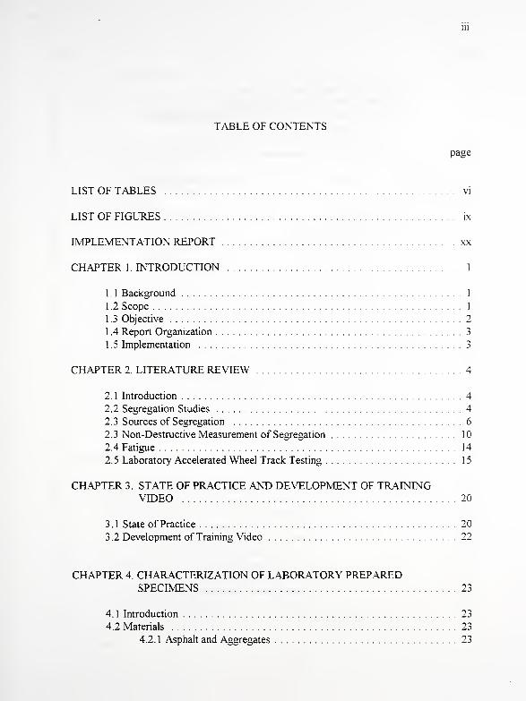
TABLE OF CONTENTS
page
LIST OF TABLES vi
LIST OF FIGURES ix
IMPLEMENTATION REPORT xx
CHAPTER 1 INTRODUCTION 1
1 .
1
Background 1
1 .2 Scope 1
1.3 Objective 2
1 .4 Report Organization 3
1.5 Implementation 3
CHAPTER 2. LITERATURE REVIEW 4
2.1 Introduction 4
2.2 Segregation Studies 4
2.3 Sources of Segregation 6
2.3 Non-Destructive Measurement of Segregation 10
2.4 Fatigue 14
2.5 Laboratory Accelerated Wheel Track Testing 15
CHAPTER 3. STATE OF PRACTICE AND DEVELOPMENT OF TRAININGVIDEO 20
3.1 State of Practice 20
3.2 Development of Training Video 22
CHAPTER 4. CHARACTERIZATION OF LABORATORY PREPAREDSPECIMENS 23
4.1 Introduction 23
4.2 Materials 23
4.2. 1 Asphalt and Aggregates 23
page
4.2.2 Asphalt Mixtures 23
4.3 Laboratory Segregation Techniques 24
4.4 Characterization of Segregated Mixtures 25
4.4.1 Segregated Mixture Asphalt Content/Gradation 26
4.4.2 Density and Air Voids 26
4.5 Laboratory Specimens for Non-Destructive Testing 27
4.5.
1
Specimen Preparation 27
CHAPTER 5 NON-DESTRUCTIVE TESTING FOR SEGREGATION 44
5.1 Introduction 44
5.2 Thermal Imaging 44
5.3 Water or Air Permeability 44
5.4 Moisture/Density Nuclear Gauge 45
5 4. 1 Calibration 46
5.4.2 Moisture (Asphalt) Content and Density 47
5.4.3 Test Procedure Discussion 47
5.4.4 Correction Factors 49
5.4.5 Nuclear Density 53
5.4.6 Nuclear Asphalt Content Discussion 56
5.4.7 Classification Procedure 59
5.5 Permittivity 61
5.5.1 Permittivity Theory 61
5.5.2 Laboratory Measurement of Permittivity 63
CHAPTER 6. FIELD TESTS 95
6 1 Introduction 95
6.2 Field Tests 95
6.2.
1
Preliminary Field Tests 97
6.2.2 Expanded Field Tests 97
6.3 Laboratory Analysis 98
6.3.1 Density 98
6.3.1.1 Bulk Density Evaluation 99
6.3.1.2 Volumetric Density 99
6.3.1.3 Comparison of Different Densities: RandomLocations 100
6.3.1.3.1 Delphi Project 100
6.3.1.3.2 Holland Project 101
6.3.1.3.3 Vincennes Project 101
6.3.1.4 Comparison of Different Densities: Visual
Locations 102
6.3.2 Asphalt Content 103
6.3.3 Gradation 1 03
page
6.4 Classification 1 04
CHAPTER 7. FLEXURAL FATIGUE TESTING OF SEGREGATEDMIXTURES 126
7.
1
Introduction 1 26
7.2 Preparation of Samples for Fatigue Testing 126
7.3 Test Apparatus 1 28
7.4 Test Procedures 128
7.5 Fatigue Test Results 1 29
7.6 Analysis 130
7.7 Performance Comparison of Different Levels of Segregation 132
CHAPTER 8. LABORATORY ACCELERATED WHEEL TRACKTESTING 146
8.1 Introduction 146
8.2 Test Apparatus 146
8.2.1 Purdue University Wheel Test Device 146
8.3 Sample Preparation 147
8.4 Test Parameters 149
8.5 Design of Experiment 150
8.6 Test Results 1 50
8.7 Analysis 151
8.7.
1
Gravel Surface Mixture 1 52
8.7.2 Limestone Surface Mixture 1 53
8.7.3 Gravel Binder Mixture 1 54
8.7.4 Limestone Binder Mixture 155
8.8 Effect of Segregation on Wheel Track Testing Performance 155
CHAPTER 9. CONCLUSIONS AND RECOMMENDATIONS 188
9.1 Characterization of Segregation 188
9.2 State of Practice 1 88
9.3 Non-Destructive Detection of Segregation 1 89
9.3.1 Thermal Imaging and Air or Water Permeameter 1 89
9.3.2 Nuclear Gauge 1 89
9.3.3 Permittivity 191
9.4 Field Conclusions 191
9.4.1 Sublot Testing Transverse to Laydown Direction 191
9.4.2 Visual Location of Segregation 192
9.5 Fatigue Characteristics 193
9.6 Permanent Deformation 1 94
page
9.7 Performance of Segregated Mixtures 195
9.8 Recommendations for Further Study 1 95
9.8.1 Non-Destructive Testing Technology 196
9.8.2 Laboratory Accelerated Wheel Track Testing 196
9.8.3 Paving Laydown Equipment 197
9.8.4 Quality Control/Quality Assurance 197
9.8.5 Gradation Limits 198
LIST OF REFERENCES 201
APPENDICE 205
A 206
B 252
C 258
D 276
E 285
LIST OF TABLES
Table page
2.
1
Test Parameters of the LCPC French Rut Tester (Parti et al.. 1995 and
Colorado Department of Transportation, 1996) 17
2.2 Georgia Loaded Wheel Tester (Lai, 1994) 18
2.3 Hamburg Steel Wheel Tracking Device (Hamburg Road Authority,
1992) 19
4.
1
Asphalt Cement Properties 29
4.2 Aggregate Characteristics 30
4.3 Optimum Surface Mixture Characteristics 31
4.4 Optimum Binder Mixture Characteristics 32
4.5 Segregation Proportions for Surface Mixtures 33
4.6 Segregation Proportions for Binder Mixtures 33
4.7 Segregated Mixture Asphalt Contents 34
4.8 Segregated Mixture Gyratory Density, Mg/m3 34
4.9 Segregated Mixture Air Voids 35
4.10 Surface Mixture Design of Experiment 35
4. 1
1
Binder Mixture Design of Experiment 36
5.1 Mean and Standard Deviation of Five Readings with Nuclear Gauge for
Asphalt Base Samples 64
5.2 Mean and Standard Deviation of Five Readings with Nuclear Gauge for
Concrete Base Samples 64
Table page
5.3 PLC Compaction Ranges 65
5.4 Density Correction Factors 65
5.5 Asphalt Content Correction Factors 65
5.6 Values of Permittivity of Some Common Materials 66
6.1 Characterization of Delphi Field Samples and Field Tests 106
6.2 Characterization of Holland Field Samples and Field Tests 107
6.3 Characterization of Vincennes Field Samples and Field Tests 108
6.4 Statistical Summary of Delphi Sublot #1, Transverse Density Data 109
6.5 Statistical Summary of Delphi Sublot #2, Transverse Density Data 109
6.6 Statistical Summary of Holland, Transverse Density Data 109
6.7 Statistical Summary of Vincennes Sublot #1, Transverse Density
Data 110
6.8 Statistical Summary of Vincennes Sublot #2, Transverse Density
Data 110
6.9 Statistical Summary of Delphi Visually Identified Segregation Density
Data 110
6. 10 Statistical Summary of Vincennes Visually Identified Segregation
Density Data Ill
6. 1
1
Discriminant Analysis: Visual Segregation Classification Ill
7 1 Surface Gravel, Very Fine Segregation Fatigue Test Results 134
7.2 Surface Gravel, Fine Segregation Fatigue Test Results 134
7.3 Surface Gravel, Control Segregation Fatigue Test Results 135
7.4 Surface Gravel, Coarse Fine Segregation Fatigue Test Results 135
Table page
7.5 Surface Gravel, Very Coarse Segregation Fatigue Test Results 136
7.6 Binder Gravel, Very Fine Segregation Fatigue Test Results 136
7.7 Binder Gravel, Fine Segregation Fatigue Test Results 137
7.8 Binder Gravel, Control Segregation Fatigue Test Results 137
7.9 Binder Gravel, Coarse Fine Segregation Fatigue Test Results 138
7.10 Binder Gravel, Very Coarse Segregation Fatigue Test Results 138
7.11 Statistical Values for Individual Level of Segregation Regression
Models 139
7.12 Values of Regression Constants B and C for N, Prediction Models 140
7.13 Statistical Values for Level of Segregation Regression Models 140
7.14 Effect of Level of Segregation on Fatigue Performance 141
8.
1
PTD and HWST Operating Characteristics 158
8.2 Wheel Track Testing Design of Experiment 159
8.3 Gravel Surface Sample Characteristics 1 59
8.4 Limestone Surface Sample Characteristics 160
8.5 Gravel Binder Sample Characteristics 160
8.6 Limestone Binder Sample Characteristics 161
8.7 Gravel Surface Wheel Tracking Test Results Summary 162
8.8 Limestone Surface Wheel Tracking Test Results Summary 163
8.9 Gravel Binder Wheel Tracking Test Results Summary 164
8.10 Limestone Binder Wheel Tracking Test Results Summary 165
8.1
1
Summary of Statistical Analysis for Rate of Deformation 166

Table page
8.12 Summary of Statistical Analysis for Creep Rate 166
8.13 Summary of Statistical Analysis for Stripping Rate 166
8.14 Gravel Binder Wheel Track Performance 167
LIST OF FIGURES
Figure page
4.
1
Surface Mixtures Gradation 37
4.2 Binder Mixtures Gradation 37
4.3 Mixing 2000 g of Control Mix 38
4.4 Transferring Control Mix to Sieve 38
4.5 Segregating Hot Mix Over Sieve 39
4.6 Transferring Coarse Fraction to Pan 39
4.7 Transferring Fine Fraction to Pan 40
4.8 Resulting Fractions from Segregation Sieving 40
4.9 Segregated Gravel Surface Mixture Gradations 41
4.10 Segregated Gravel Binder Mixture Gradations 41
4.11 Segregated Limestone Surface Mixture Gradations 42
4.12 Segregated Limestone Binder Mixture Gradations 42
4.13 Purdue Linear Compactor (PLC) 43
4.14 Schematic of Hidden Segregation 43
5.1 Air Permeameter 67
5.2 Permeability: #1 1 Surface Gravel, 50 mm Surface Segregation, Asphalt
Base 67
5.3 Permeability: #1 1 Surface Gravel, 50 mm Surface Segregation, Concrete
Base 68
Figure page
5.4 Permeability: #1 1 Surface Gravel, Hidden Segregation. Asphalt
Base 68
5.5 Permeability: #1 1 Surface Gravel, Hidden Segregation, Concrete
Base 69
5.6 Permeability: #1 1 Surface Limestone, Hidden Segregation, Asphalt
Base 69
5.7 Permeability: #1 1 Surface Limestone, Hidden Segregation, Concrete
Base 70
5.8 Permeability: #8 Binder Gravel. Hidden Segregation, Asphalt
Base 70
5.9 Permeability: #8 Binder Gravel, Hidden Segregation. Concrete
Base 71
5.10 Permeability: #8 Binder Limestone, Hidden Segregation, Asphalt
Base 71
5.11 Permeability: #8 Binder Limestone, Hidden Segregation, Concrete
Base 72
5.12 Nuclear Gauge 72
5.13 Nuclear Gauge Number of Readings 73
5.14 Nuclear Density Bias Plot - #1 1 Gravel 73
5.15 Nuclear Density Bias Plot - #1 1 Limestone 74
5.16 Nuclear Density Bias Plot - #8 Gravel 74
5.17 Nuclear Density Bias Plot - #8 Limestone 75
5 18 Nuclear Asphalt Content Bias Plot - #1 1 Gravel 75
5.19 Nuclear Asphalt Content Bias Plot - #1 1 Limestone 76
5.20 Nuclear Asphalt Content Bias Plot - #8 Gravel 76
Xlll
Figure page
5.21 Nuclear Asphalt Content Bias Plot - #8 Limestone 77
5.22 Nuclear Density - Asphalt Base - #1 1 Gravel 77
5.23 Nuclear Density - Concrete Base - #1 1 Gravel 78
5.24 Nuclear Density - Asphalt Base - #1 1 Limestone : 78
5.25 Nuclear Density - Concrete Base - #1 1 Limestone 79
5.26 Nuclear Density - Asphalt Base - #8 Gravel 79
5.27 Nuclear Density - Concrete Base - #8 Gravel 80
5.28 Nuclear Density - Asphalt Base - #8 Limestone 80
5.29 Nuclear Density - Concrete Base 81
5.30 Nuclear Asphalt Content - Asphalt Base - #11 Gravel 81
5.31 Nuclear Asphalt Content - Concrete Base - #1 1 Gravel 82
5.32 Nuclear Asphalt Content - Asphalt Base - #1 1 Limestone 82
5.33 Nuclear Asphalt Content - Concrete Base - #1 1 Limestone 83
5.34 Nuclear Asphalt Content - Asphalt Base - #8 Gravel 83
5.35 Nuclear Asphalt Content - Concrete Base - #8 Gravel 84
5.36 Nuclear Asphalt Content - Asphalt Base - #8 Limestone 84
5.37 Nuclear Asphalt Content - Concrete Base - #8 Limestone . 85
5.38 Laboratory Dielectric Constant Measurement Equipment 85
5.39 Frequency vs. Magnitude Transmission Coefficients, #1 1 Surface
Gravel, Very Fine 86
XIV
Figure page
5.40 Frequency vs. Magnitude Transmission Coefficients, #1 1 Surface
Gravel, Control 86
5.41 Frequency vs. Magnitude Transmission Coefficients, #1 1 Surface
Gravel, Very Coarse 87
5.42 Frequency vs. Magnitude Transmission Coefficients, #8 Binder
Gravel, Very Fine 87
5.43 Frequency vs. Magnitude Transmission Coefficients, #8 Binder
Gravel, Control 88
5.44 Frequency vs. Magnitude Transmission Coefficients, #8 Binder
Gravel, Very Coarse 88
5.45 Frequency vs. Phase Transmission Coefficients, #1 1 Surface Gravel,
Very Fine 89
5.46 Frequency vs. Phase Transmission Coefficients, #1 1 Surface Gravel,
Control 89
5 .47 Frequency vs. Phase Transmission Coefficients, #1 1 Surface Gravel,
Very Coarse 90
5.48 Frequency vs. Phase Transmission Coefficients, #8 Binder Gravel,
Very Fine 90
5.49 Frequency vs. Phase Transmission Coefficients, #8 Binder Gravel,
Control 91
5.50 Frequency vs. Phase Transmission Coefficients, #8 Binder Gravel,
Very Coarse 91
5.51 Dielectric Constant Measurement, #1 1 Surface Gravel. Very Fine 92
5.52 Dielectric Constant Measurement, #1 1 Surface Gravel. Control 92
5.53 Dielectric Constant Measurement, #1 1 Surface Gravel, Very
Coarse 93
5.54 Dielectric Constant Measurement, #8 Binder Gravel, Very Fine 93
XV
Figure page
5.55 Dielectric Constant Measurement, #8 Binder Gravel, Control 94
5.56 Dielectric Constant Measurement, #8 Binder Gravel, Very Coarse 94
6.
1
Ft Wayne, All Density Data, 1 Minute Reading 112
6.2 Ft. Wayne, All Density Data, 4 Minute Reading 112
6.3 Ft. Wayne, All Moisture (Asphalt) Content Data, 1 Minute
Reading 113
6.4 Ft. Wayne, All Moisture (Asphalt) Content Data, 4 Minute
Reading 113
6.5 Delphi, Sublot #1, Density, 4 Minute Reading 114
6.6 Delphi, Sublot #2, Density, 4 Minute Reading 114
6.7 Holland, Density, 4 Minute Reading 115
6.8 Vincennes, Sublot #1, Density, 4 Minute Reading 115
6.9 Vincennes, Sublot #2, Density, 4 Minute Reading 116
6.10 Delphi, Sublot #1, Random Location, Density Comparisons 116
6.1
1
Delphi, Sublot #2, Random Location, Density Comparisons 117
6.12 Holland, Random Location, Density Comparisons 117
6.13 Vincennes, Sublot #1, Random Location, Density Comparisons 118
6.14 Vincennes, Sublot #2, Random Location, Density Comparisons 118
6.15 Delphi, Visual Locations, Density Comparisons 119
6.16 Vincennes, Visual Locations, Density Comparisons 119
6.17 Delphi, Sublot #1, Moisture (Asphalt) Content, 4 Minute Reading 120
6.18 Delphi, Sublot #2, Moisture (Asphalt) Content, 4 Minute Reading 120
Figure page
6.19 Holland, Moisture (Asphalt) Content, 4 Minute Reading 121
6.20 Vincennes, Sublot #1, Moisture (Asphalt) Content, 4 Minute
Reading 121
6.21 Vincennes, Sublot #2, Moisture (Asphalt) Content, 4 Minute
Reading 122
6.22 Delphi, Sublot #1, Difference in Gradation on the 9.5 mm Sieve 122
6.23 Delphi, Sublot #2, Difference in Gradation on the 9.5 mm Sieve 123
6.24 Holland, Difference in Gradation on the 4.75 mm Sieve 123
6.25 Vincennes, Sublot #1, Difference in Gradation on the 9.5 mmSieve 1 24
6.26 Vincennes, Sublot #2, Difference in Gradation on the 9.5 mmSieve 124
6.27 Coarse Segregation Classification Probability (#8 Binder, Greater than
-5% Difference on the 9.5 mm Sieve) 125
7.
1
Purdue Linear Compactor and Infrared Heater 142
7.2 Concrete Saw 142
7.3 First Phase of Saw Cutting Beams, Top View 143
7 4 Second Phase of Saw Cutting Beams, Side View 143
7.5 MTS Test System 144
7.6 Repeated Flexural Frame in the Environmental Chamber 144
7.7 Flexural Fatigue Prediction Results, Gravel Surface Mixture 145
7.8 Flexural Fatigue Prediction Results, Gravel Binder Mixture 145
8.1 Purdue Linear Compactor and Infrared Heater 168

XVII
Figure page
8.2 Location of Sample Height Measurements from a Planimetric
View 1 68
8.3 Contact Area of 682 kPa Tire Pressure and 150 kg Load 169
8.4 Contact Area of 682 kPa Tire Pressure and 175 kg Load 169
8.5 Wheel Track Test Results of Gravel Surface Mixture, Control,
Sample 1 1 70
8.6 Wheel Track Test Results of Gravel Surface Mixture, Control.
Sample 2 1 70
8.7 Wheel Track Test Results of Gravel Surface Mixture, Control,
Sample 3 171
8.8 Wheel Track Test Results of Gravel Surface Mixture, Coarse,
Sample 1 171
8.9 Wheel Track Test Results of Gravel Surface Mixture, Coarse,
Sample 2 1 72
8.10 Wheel Track Test Results of Gravel Surface Mixture, Coarse,
Sample 3 1 72
8. 1
1
Wheel Track Test Results of Gravel Surface Mixture, Very Coarse,
Sample 1 1 73
8.12 Wheel Track Test Results of Gravel Surface Mixture, Very Coarse,
Sample 2 1 73
8. 13 Wheel Track Test Results of Gravel Surface Mixture, Very Coarse,
Sample 3 1 74
8.14 Wheel Track Test Results of Limestone Surface Mixture, Control,
Sample 1 1 74
8.15 Wheel Track Test Results of Limestone Surface Mixture, Control,
Sample 2 175
8. 16 Wheel Track Test Results of Limestone Surface Mixture, Control,
Sample 3 175
Figure page
8.17 Wheel Track Test Results of Limestone Surface Mixture. Coarse.
Sample 1 1 76
8.18 Wheel Track Test Results of Limestone Surface Mixture, Coarse.
Sample 2 1 76
8. 19 Wheel Track Test Results of Limestone Surface Mixture. Coarse,
Sample 3 1 77
8.20 Wheel Track Test Results of Limestone Surface Mixture, Very Coarse.
Sample 1 1 77
8.21 Wheel Track Test Results of Limestone Surface Mixture, Very Coarse.
Sample 2 1 78
8.22 Wheel Track Test Results of Limestone Surface Mixture, Very Coarse,
Sample 3 1 78
8.23 Wheel Track Test Results of Gravel Binder Mixture, Control,
Sample 1 1 79
8.24 Wheel Track Test Results of Gravel Binder Mixture, Control,
Sample 2 1 79
8.25 Wheel Track Test Results of Gravel Binder Mixture, Control,
Sample 3 1 80
8.26 Wheel Track Test Results of Gravel Binder Mixture, Coarse,
Sample 1 180
8.27 Wheel Track Test Results of Gravel Binder Mixture, Coarse,
Sample 2 181
8.28 Wheel Track Test Results of Gravel Binder Mixture, Coarse,
Sample 3 181
8.29 Wheel Track Test Results of Gravel Binder Mixture, Very Coarse,
Sample 1 1 82
8.30 Wheel Track Test Results of Gravel Binder Mixture, Very Coarse,
Sample 2 182
XIX
Figure page
8.3
1
Wheel Track Test Results of Gravel Binder Mixture, Very Coarse,
Sample 3 183
8.32 Wheel Track Test Results of Limestone Binder Mixture, Control,
Sample 1 183
8.33 Wheel Track Test Results of Limestone Binder Mixture, Control,
Sample 2 1 84
8.34 Wheel Track Test Results of Limestone Binder Mixture, Control,
Sample 3 1 84
8.35 Wheel Track Test Results of Limestone Binder Mixture, Coarse,
Sample 1 185
8.36 Wheel Track Test Results of Limestone Binder Mixture, Coarse,
Sample 2 185
8.37 Wheel Track Test Results of Limestone Binder Mixture, Coarse,
Sample 3 1 86
8.38 Wheel Track Test Results of Limestone Binder Mixture, Very Coarse,
Sample 1 1 86
8.39 Wheel Track Test Results of Limestone Binder Mixture, Very Coarse.
Sample 2 187
8.40 Wheel Track Test Results of Limestone Binder Mixture, Very Coarse,
Sample 3 187
9.
1
Visual Coarse Segregation 199
9.2 Visual Coarse Segregation Classification Based on 4 Minute Nuclear
Gau«e Readings 204

IMPLEMENTATION REPORT
This research project has demonstrated that nuclear gauge testing of visually
identified segregated areas is very effective in quantifying segregation and should be
implemented. Based upon field testing with four minute nuclear gauge readings of
density and moisture (asphalt) content, coarse segregation was identified with perfect
accuracy. The following implementation of nuclear gauge testing to confirm visual
A standard background count is taken before use on a daily basis to check
gauge operation and allow for source decay. The new count will pass if
plus or minus two percent of the moisture average and/or plus or minus
one percent of the density average. The operating manual should be
consulted to ensure safe operating procedures.
The gauge is operated in backscatter mode Further, the gauge is operated
in the soil mode allowing for both density and moisture (asphalt) content
measurements.
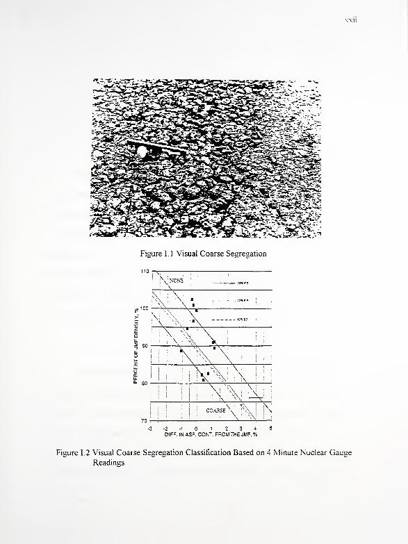
Analysis of coarse segregation is visually identified by an inspector. This
area of coarse segregation is defined as an area having considerably more
coarse aggregate than the surrounding acceptable mat and contains little
or no mastic. Figure II identifies such an area.

A nuclear gauge is placed on the subject location and concurrent four
minute readings of density and moisture (asphalt) content are recorded
The density reading is subtracted from the job mix formula target density.
This value is referred to as the "Difference in density from the JiVLF."
The moisture (asphalt) content reading is subtracted from the job mix
formula target asphalt content. This value is referred to as the "Difference
in asphalt content from the JMF "
The values obtained in steps 5 and 6 are plotted on Figure 1.2 titled
"Visual Coarse Segregation Classification Based on 4 Minute Nuclear
Gauge Readings."
If the plotted point falls below the 90 percent posterior probability line (90
PP), the location is identified as being coarsely se<zre<iated.
XX11
T.~~Z-
Figure 1. 1 Visual Coarse Segregation
w2Mi
cu.
^ 90u.O
N; , , ,
: \\ j
i \ j
\
:\\\:i !
; W''\:V;4 ;\ j i i
Ill III KKiCOARSE v !
.
'
! 1 ! ' ! IN UM•3-2-10123*5
DIFF. IN ASP. CONT. FROM THE JMF, %
Figure 1.2 Visual Coarse Segregation Classification Based on 4 Minute Nuclear Gauge
Readings
CHAPTER 1. INTRODUCTION
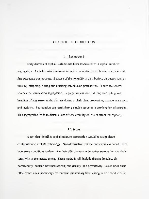
] 1 Background
Early distress of asphalt surfaces has been associated with asphalt mixture
segregation. Asphalt mixture segregation is the nonuniform distribution of coarse and
fine aggregate components. Because of the nonuniform distribution, distresses such as
raveling, stripping, rutting and cracking can develop prematurely. There are several
sources that can lead to segregation. Segregation can occur during stockpiling and
handling of aggregate, in the mixture during asphalt plant processing, storage, transport.
and laydown Segregation can result from a single source or a combination of sources
This segregation leads to distress, loss of serviceability or loss of structural capacity
1.2 Scope
A test that identifies asphalt mixture segregation would be a significant
contribution to asphalt technology. Non-destructive test methods were examined under
laboratory conditions to determine their effectiveness in detecting segregation and their
sensitivity in the measurement. These methods will include thermal imaging, air
permeability, nuclear moisture( asphalt) and density, and permittivity. Based upon their
effectiveness in a laboratory environment, preliminary field testing will be conducted to

evaluate their sensitivity under field conditions.
Equally important to detecting segregation is the impact of segregation on
pavement performance The performance of mixtures with varying levels of segregation
were determined through repeated flexural and accelerated wheel track testing.
1.3 Objective
Objectives of this study include: 1. characterization of segregated mixtures. 2.
identification of a technology or combination of technologies that detects segregation, 3.
implementation of this technology, and 4. establishment of the relative reduction in
pavement performance due to segregation. This study will involve both laboratory and
field investigations. The following tests and evaluations are planned on laboratory
prepared specimens:
i.) Gradation analyses.
ii.) Density and asphalt content determination.
iii.) Air voids analyses.
iv.) Nuclear moisture (asphalt) content and density measurements
v.) Repeated flexural testing.
vi.) Accelerated wheel track testing.
The following tests will be performed on field specimens:
i.) Nuclear moisture (asphalt) content and density measurements.
ii.) Density and asphalt content determination.

iii.) Gradation analyses.
1 .4 Report Organization
Chapter two discusses the literature review on segregation, its measurement and
effect. Chapter three provides a summary of the state of practice survey results and the
development of the training video. Chapter four evaluates potential technologies and
their effectiveness to detect segregation. Chapter five describes the technologies studied
in a laboratory environment to detect segregation. Chapter six explains the field data
collection and describes laboratory tests on field cores. Fatigue testing of segregated
mixtures is discussed in Chapter seven. Chapter eight covers the accelerated wheel track
testing of segregated mixtures The conclusions of the study with recommendations for
future research are outlined in Chapter nine.
1.5 Implementation
Implementation of the results and recommendations in this study is expected to
assist INDOT in detecting segregated mixtures. Further, reduction in pavement
performance based upon degree of segregation will be established for some mixtures
This will assist INDOT in implementing a more effective quality control/quality
assurance program. Overall this will result in tax dollar savings.
CHAPTER 2: LITERATURE REVIEW
2.1 Introduction
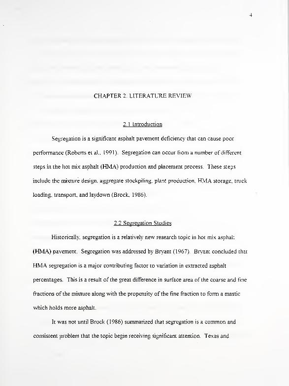
Segregation is a significant asphalt pavement deficiency that can cause poor
performance (Roberts et al., 1991 ). Segregation can occur from a number of different
steps in the hot mix asphalt (HMA) production and placement process. These steps
include the mixture design, aggregate stockpiling, plant production, HMA storage, truck
loading, transport, and laydown (Brock, 1986).
2.2 Segregation Studies
Historically, segregation is a relatively new research topic in hot mix asphalt
(HMA) pavement. Segregation was addressed by Bryant (1967). Bryant concluded that
HMA segregation is a major contributing factor to variation in extracted asphalt
percentages. This is a result of the great difference in surface area of the coarse and fine
fractions of the mixture along with the propensity of the fine fraction to form a mastic
which holds more asphalt.
It was not until Brock (1986) summarized that segregation is a common and
consistent problem that the topic begin receiving significant attention. Texas and
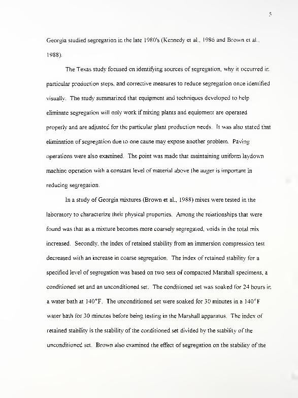
Georgia studied segregation in the late 1980's (Kennedy et al.. 1986 and Brown et al..
1988).
The Texas study focused on identifying sources of segregation, why it occurred in
particular production steps, and corrective measures to reduce segregation once identified
visually. The study summarized that equipment and techniques developed to help
eliminate segregation will only work if mixing plants and equipment are operated
properly and are adjusted for the particular plant production needs. It was also stated that
elimination of segregation due to one cause may expose another problem. Paving
operations were also examined. The point was made that maintaining uniform laydown
machine operation with a constant level of material above the auger is important in
lg segregation.
In a study of Georgia mixtures (Brown et al., 1988) mixes were tested in the
laboratory to characterize their physical properties. Among the relationships that were
found was that as a mixture becomes more coarsely segregated, voids in the total mix
increased. Secondly, the index of retained stability from an immersion compression test
decreased with an increase in coarse segregation. The index of retained stability for a
specified level of segregation was based on two sets of compacted Marshall specimens, a
conditioned set and an unconditioned set. The conditioned set was soaked for 24 hours in
a water bath at 140°F. The unconditioned set were soaked for 30 minutes in a 140°F
water bath for 30 minutes before being testing in the Marshall apparatus. The index of
retained stability is the stability of the conditioned set divided by the stability of the
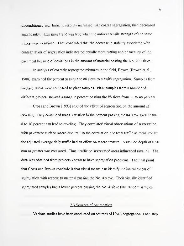
unconditioned set. Initially, stability increased with coarse segregation, then decreased
significantly. This same trend was true when the indirect tensile strength of the same
mixes were examined. They concluded that the decrease in stability associated with
coarser levels of segregation indicates potentially more rutting and/or raveling of the
pavement because of deviations in the amount of material passing the No. 200 sieve.
In analysis of coarsely segregated mixtures in the field. Brown (Brown et al..
1988) examined the percent passing the #8 sieve to classify segregation Samples from
in-place HMA were compared to plant samples. Plant samples from a number of
different projects showed a range in percent passing the #8 sieve from 33 to 48 percent
Cross and Brown (1993) studied the effect of segregation on the amount of
raveling. They concluded that a variation in the percent passing the #4 sieve greater than
8 to 10 percent can lead to raveling. They correlated visual observations of segregation
with pavement surface macro-texture. In the correlation, the total traffic as measured by
the adjusted average daily traffic had an effect on macro texture. A raveled depth of 0.50
mm or greater was measured. Thus, traffic on segregated areas influenced raveling. The
data was obtained from projects known to have segregation problems. The final point
that Cross and Brown conclude is that visual means can identify the lateral extent of
segregation with respect to material passing the No. 4 sieve. Their visually identified
segregated samples had a lower percent passing the No. 4 sieve than random samples
2.3 Sources of Segregation
Various studies have been conducted on sources ofHMA segregation. Each step
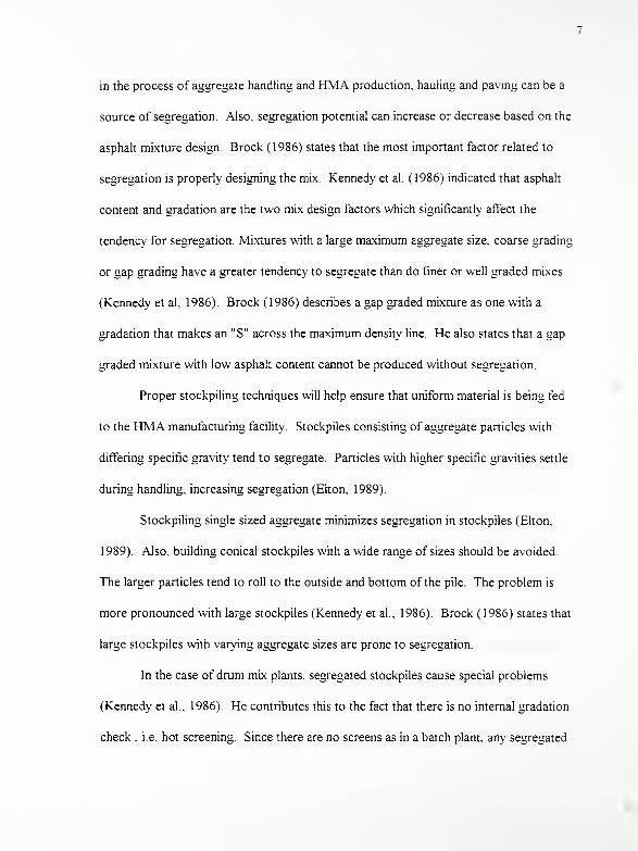
in the process of aggregate handling and HMA production, hauling and paving can be a
source of segregation. Also, segregation potential can increase or decrease based on the
asphalt mixture design. Brock (1986) states that the most important factor related to
segregation is properly designing the mix. Kennedy et al. (1986) indicated that asphalt
content and gradation are the two mix design factors which significantly affect the
tendency for segregation. Mixtures with a large maximum aggregate size, coarse grading
or gap grading have a greater tendency to segregate than do finer or well graded mixes
(Kennedy et al, 1986). Brock (1986) describes a gap graded mixture as one with a
gradation that makes an "S" across the maximum density line. He also states that a gap
graded mixture with low asphalt content cannot be produced without segregation.
Proper stockpiling techniques will help ensure that uniform material is being fed
to the HMA manufacturing facility. Stockpiles consisting of aggregate particles with
differing specific gravity tend to segregate. Particles with higher specific gravities settle
during handling, increasing segregation (Elton, 1989).
Stockpiling single sized aggregate minimizes segregation in stockpiles (Elton.
1989). Also, building conical stockpiles with a wide range of sizes should be avoided.
The larger particles tend to roll to the outside and bottom of the pile. The problem is
more pronounced with large stockpiles (Kennedy et al., 1986). Brock ( 1 986) states that
large stockpiles with varying aggregate sizes are prone to segregation.
In the case of drum mix plants, segregated stockpiles cause special problems
(Kennedy et al., 1986). He contributes this to the fact that there is no internal gradation
check , i.e. hot screening. Since there are no screens as in a batch plant, any segregated
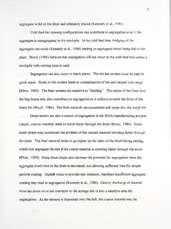
aggregate is fed to the plant and ultimately placed (Kennedy et al ., 1986).
Cold feed bin opening configurations can contribute to segregation even if the
aggregate is unsegregated in the stockpile. In the cold feed bins, bridging of the
aggregate can occur (Kennedy et al., 1986) leading to segregated mixes being fed to the
plant. Brock (1986) believes that segregation will not occur at the cold feed bins unless a
stockpile with varying sizes is used.
Segregation can also occur in batch plants. The hot bin screens must be kept in
good repair. Holes in the screens leads to contamination of the next largest size range
(Elton, 1989). The finer screens are sensitive to "blinding". The return of the fines from
the bag house may also contribute to segregation as it collects towards the front of the
finest bin (Brock, 1986). The finer material can accumulate and surge into the weigh bin
Drum mixers are also a source of segregation in the HMA manufacturing process
Larger, coarser material tends to travel faster through the drum (Brock, 1986). Steep
drum slopes may accentuate the problem of the coarser material traveling faster through
the plant. The finer material tends to go higher up the sides of the drum during mixing,
which will segregate the mix if the coarse material is traveling faster through the drum
(Elton, 1989). Steep drum slopes also increase the potential for segregation since the
aggregate dwell time in the drum is decreased, not allowing sufficient time for proper
particle coating. Asphalt tends to provide mix cohesion, therefore insufficient aggregate
coating may lead to segregation (Kennedy et al., 1986). Gravity discharge of material
from the drum on to the conveyor to the storage silo is also a sensitive area for
segregation. As the mixture is deposited onto the belt, the coarse material may be
deposited on one side of the belt with the fine material deposited on the other
The process of conveying HMA to the surge silos can contribute to segregation.
A ladder or drag conveyor is generally used to deliver freshly mixed HMA from the drum
to the storage silo. Segregation will usually not occur on a drag conveyor unless there is
"hydroplaning" or the mix is segregated as it is fed onto the drag conveyor (Brock.
1986). "Hydroplaning" is caused when the drag conveyor is cold and a buildup of fine
material occurs on the flights. This buildup will cause the coarse material of fresh HMA
to spill backwards down the conveyor rather than move up the conveyor with the fine
fraction as a uniform mixture (Brock, 1986).
There are conditions associated with the surge bins or storage silos which may
contribute to segregation. One main concern is proper placement of the mix into the silo.
This placement can be achieved with a bin loader or batcher, or a rotating chute (Elton,
1 989). A bin loader allows mix to accumulate in a bin above the storage silo until it
reaches its capacity, then drops the mix into the silo as a batch. A rotating chute is a
continuous feed device that keeps the material being fed into the storage silo from
collecting in a cone in the middle of the bin. Problems can arise during loading of the
storage silo with a rotating chute if the end of the chute wears away. The material
entering the silo will have a horizontal trajectory rather than a vertical one and coarse
material will collect on the outside of the bin (Kennedy et al., 1986). The amount of
material kept in the storage silo can also significantly affect segregation Kennedy et al
(1986) suggested keeping the silos at least one third full at all times. Brock ( 1 986) also
recommends not allowing the material to fall below the top of the bottom cone during bin

10
discharge.
Truck segregation is likely to occur if the trucks are loaded incorrectly from the
storage silo (Brock, 1986) Coarse material will collect towards the outside walls of the
truck if the truck is not loaded in distributed batches, i.e. one drop in the front of the
truck, one in the back and one in the middle (Kennedy et al., 1986). This segregated
material will then be fed directly to the paver resulting in a segregated area between each
truck load of material (Kennedy et al., 1986).
Even when material is successfully processed through all of the steps of HMA
production segregation can still occur in the HMA paving machine (Brock, 1986) Areas
of concern include operation of the paver wings; auger operation including condition and
speed; proper flooding of the hopper; truck loading; and proper adjustment of the screed
(Kennedy et al., 1986).
2.4 Non-Destructive Measurement of Segregation
Permeability has been used in the past to detect areas of segregation Zube ( 1 962)
showed that dense-graded HMA pavements became highly permeable to water, 1 .3
mm/sec, at approximately 8 percent air voids. Above 8 percent air voids, the
permeability increases quickly. Brown et al. (1989) in a study of segregated mixes
showed that HMA mixtures were impermeable to water as long as the air void content
was below approximately 8 percent.
Nuclear gauges have been studied and used as a quality control device in the
asphalt industry for many years (Belt et al., 1991). However, most studies have used

1
1
nuclear density and asphalt content independent of each other. Nuclear gauges have the
advantage of rapidly and non-destructively measuring pavement densities (NAPA. 1991).
Duncan (1996) conducted a laboratory study using a nuclear moisture/density gauge and
concluded that the gauge can effectively identify variations in asphalt mixture physical
properties attributed to segregation. Several researchers have concluded that the nuclear
gauge accurately measures density when compared with densities of cores, i.e. Kennedy
et al. (1989) and the Missouri Highway and Transportation Department ( 1991
)
Studies using a nuclear gauge to determine asphalt content were performed by
Regan (1975) and Christensen and Tarris (1989). Both studies found nuclear gauges to
produce results comparable to those of conventional extractions. However, they do warn
that the presence of absorbed moisture in aggregate can cause problems as the readings
are based on a heavy hydrogen count. The reason is the hydrogen in both water and
asphalt, a hydrocarbon, are measured cumulatively.
The State of Georgia proposed a method for using a nuclear density gauge to
detect segregation based on density variations between a suspected segregated area and
an adjacent unsegregated area. A suspect site on the pavement mat was identified
visually. The nuclear gauge in the backscatter mode was used on the surface of the
suspect site to determine the uncorrected density. The surface voids were then filled with
a fine slurry of water, sand and cement. The slurry was then covered with a plastic sheet
of Saran Wrap and the area retested. If the difference between the two readings was
greater then 10 pcf, the area was considered segregated. This method has not been
utilized by the State of Georgia since a new method was developed. The new method

Georgia has proposed utilizes the nuclear gauges void count as the governing property
concerning segregated areas. If a visually segregated pavement area has voids exceeding
9% as determined by the nuclear gauge, then the area is considered suspect and should be
removed. This procedure has not been accepted yet due to lack of supporting data to
confirm the correlation between in place air voids as determined by the nuclear gauge
and degree of segregation.
The State of Montana uses a method that is the same as the Georgia slurry
method, except that the density difference allowed is only 6 pcf before sites are
considered segregated. The Montana method is outlined in the survey form that was
submitted for data contained in Chapter 3 and is contained in Appendix A. The survey
form did not state whether the method has been accepted or is currently used in Montana
Winfrey (1990) proposed a method to detect segregation on coarse areas using the
Troxler thin-lift density gauge. The thin lift gauge is supplied with a calibration plate
upon which the gauge may be placed to eliminate surface voids error. The gauge was
used to take an initial density reading on a visually segregated area of the pavement. The
calibration plate was then placed over the coarse area and the gauge placed on top of the
plate. The gauge was placed in the surface void mode and a second reading taken. If the
measured difference in density between the two readings exceeded 9 pcf, the area was
considered segregated. This method was not in place at the time the survey outlined in
Chapter 3 was conducted, nor was it recommended by the State itself due to the lack of
data for confirmation of the procedure.
Colorado outlined a method to detect segregation with a nuclear density gauge

based on density variations in the pavement mat. The proposed procedure entailed
placing the nuclear gauge on a visually identified segregated area and taking a one
minute density count. A second density count would then be taken at an adjacent area of
the compacted pavement surface. If the density difference between the two readings was
more than 5 pcf then the pavement was considered segregated. The survey form states
that the method was seldom tried and never used as a specification.
Cross and Brown (1993) stated that if the nuclear gauge was utilized to determine
the unit weight of segregated areas of a pavement, low values will be determined which
might be useful in verifying segregation during construction.
Lackey approached the problem by measuring density profiles with nuclear
density readings (Lackey, 1986). Measured density profiles can be determined along the
lane length or across the lane width. By measuring the area to be tested in sublots. i.e a
12 ft wide paving lane measured at two foot intervals, and comparing the density reading
versus distance, a density profile can be developed. As already stated, coarsely
segregated areas of pavements have an open texture and low density.
Based on studies and applications in the literature, a nuclear density gauge can be
used to measure density differences resulting from segregation as part of construction
control. Some state agencies, Kansas and Missouri, utilize the nuclear gauge in this
manner to develop a density profile and evaluate the pavement for segregation.
Permittivity is a relatively new technology being applied to the HMA industry.
To date, there has only been one study with this technology applied to HMA. This
research was conducted by AJ-Qadi et al. (1991) on small specimens to measure the
effect of moisture on asphalt concrete at microwave frequencies. They were able to
measure moisture content with reasonable accuracy by measuring the dielectric
properties of wet and dry specimens. These specimens were tested in a reflection mode,
however the specimens were metal-backed. As a result, this technique is not currently
viable as a non-destructive field test method
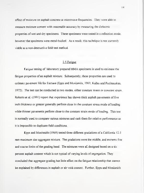
2.5 Fatigue
Fatigue testing of laboratory prepared FDVIA specimens is used to estimate the
fatigue properties of an asphalt mixture. Subsequently, these properties are used to
estimate pavement life for fracture (Epps and Monismith, 1969, Kallas and Puzinauskas.
1972). The test can be conducted in two modes, either constant stress or constant strain
Roberts et al. (1991) report that experience has shown thick asphalt pavements of five
inch thickness or greater generally perform close to the constant stress mode of loading
while thinner pavements perform close to the constant strain mode of loading. This test
is normally used to compare various mixtures and rank them for relative performance as
it is impossible to duplicate field conditions.
Epps and Monismith (1969) tested three different gradations of a California 12.5
mm maximum size aggregate mixture. The gradations were the middle, and extreme fine
and coarse limits of the grading band. The mixtures were all designed based on a six
percent asphalt content which is not typical of varying levels of segregation. They
concluded that aggregate grading has little effect on the fatigue relationship that cannot
be explained by differences in asphalt or air void content. Further, Epps and Monismith

15
concluded that the three different levels of gradation were not statistically different and
represented the three levels as a single regression line.
Khedaywi and White ( 1 996) developed a laboratory procedure for segregating an
optimum mixture. They tested a 25 mm nominal maximum aggregate size gravel mixture
at five levels of segregation. The fatigue curves (log 6 vs. log N, ) of the five levels of
segregation were linear and parallel. At a given level of strain, coarser segregated
mixtures had lower cycles to failure.
2 6 Laboratory Accelerated Wheel Track Testing
To date, there has been no documented laboratory accelerated testing of
segregated mixtures. This is likely the result of wheel track testing being a more recently
developed test The literature reveals that there has been three laboratory accelerated
wheel tracking devices used in the United States. They are considerably different in
design. These are the Laboratoire Centrale des Ponts et Chaussees (LCPC) French
Rutter, the Georgia Loaded Wheel Tester (GLWT) and the Hamburg Steel Wheel
Tracking Device (HSWT). Tables 2. 1 through 2.3 list the test conditions and parameters
for each device. Each device has used different criteria in evaluating mixture
performance. The French Rutter' s criteria of a quality mix is one that ruts less than 20
percent of the test specimen's thickness (CDOT, 1996). The GLWT's criteria is a rut
depth of 7.5 mm for 8000 wheel passes for a poor mix (Collins, 1996). And, the HSWT's
criteria is a 4mm rut depth in less than 20,000 wheel passes (Hamburg Road Authority,
1992) for failure. In application of the French Rutter, both rutting and uplift are

16
measured. The HSWT measures just rutting. Both rutting and uplift are measured during
tests with the GLWT. Literature for these wheel track testers indicate inconsistencies in
the tests. As a result, testing duplicate samples is recommended and if an inconsistency
between two tests do occur, a third sample is tested. No comparisons of equivalency
between the different test apparatus has been reported.
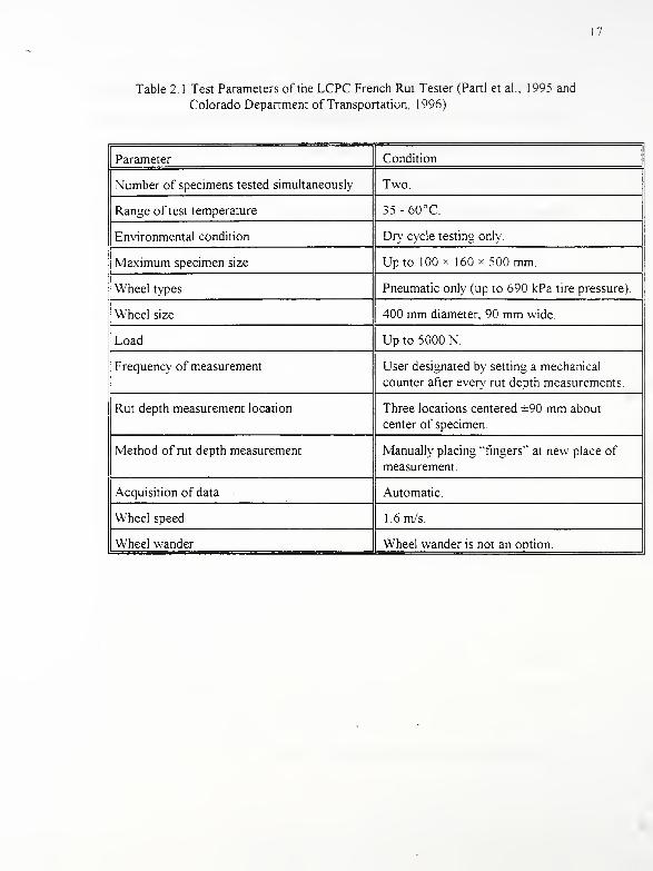
17
Table 2. 1 Test Parameters of the LCPC French Rut Tester (Parti et al., 1995 and
Colorado Department of Transportation, 1996)
Parameter Condition
Number of specimens tested simultaneously Two.
Range of test temperature 35-60°C.
Environmental condition Dry cycle testing only
Maximum specimen size Up to 100 x 160 x 500 mm.
Wheel types Pneumatic only (up to 690 kPa tire pressure)
Wheel size 400 mm diameter, 90 mm wide.
Load Up to 5000 N.
Frequency of measurement User designated by setting a mechanical
counter after every rut depth measurements
Rut depth measurement location Three locations centered =90 mm about
center of specimen.
Method of rut depth measurement Manually placing "fingers" at new place of
measurement.
Acquisition of data Automatic.
Wheel speed 1.6 m/s.
Wheel wander Wheel wander is not an option.
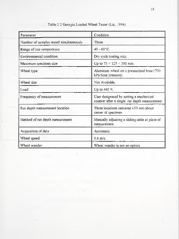
Table 2.2 Georgia Loaded Wheel Tester (Lai, 1994)
Parameter Condition
Number of samples tested simultaneously Three
Range of test temperature 40 - 60°C.
Environmental condition Dry cycle testing only.
Maximum specimen size Up to 75 x 125 - 300 mm.
Wheel type Aluminum wheel on a pressurized hose (700
kPa hose pressure)
Wheel size Not Available.
Load Up to 445 N.
Frequency of measurement User designated by setting a mechanical
counter after a single rut depth measurement.
Rut depth measurement location Three locations centered ±50 mm about
center of specimen.
Method of rut depth measurement Manually adjusting a sliding table at place of
measurement
Acquisition of data Automatic.
Wheel speed 0.6 m/s.
Wheel wander Wheel wander is not an option

19
Table 2.3 Hamburg Steel Wheel Tracking Device (Hamburg Road Authority. 1 992]
Parameter Condition
Number of samples tested simultaneously Two.
Range of test temperature 50°C.
Environmental condition Wet cycle testing only
Maximum specimen size Up to 175 x 305 x 305 mm
Wheel types Steel wheel, 47 mm wide.
Wheel size 203.5 mm.
Load Up to 697 N.
Frequency of measurement Every 250 wheel passes.
Rut depth measurement location Center of specimen.
Method of rut depth measurement Automatic by linear voltage displacement
transducers.
Acquisition of data Automatic.
Wheel speed Sinusoidal with a maximum of 0.33 m/s at the
center of sample.
Wheel wander Wheel wander is not an option.

20
CHAPTER 3 STATE OF PRACTICE AND DEVELOPMENT OF TRAJNING VIDEO
3 1 State of Practice
A survey was conducted of the 50 state departments of transportation, plus the District of
Columbia, to determine awareness of segregation, specifications or guidelines for its
prevention and any test methods for its detection. Survey forms were distributed to the
chief materials engineer for each agency. The completed survey forms for each of the
state agencies that responded are contained in Appendix A.
Forty-two of the fifty-one agencies (82%) that were sent questionnaires
responded. These results were used to establish the knowledge base and significance of
factors relating to segregation.
The main areas addressed in the survey were:
1
.
Agency specifications for prevention or minimization of
segregation.
2. Agency training for segregation prevention techniques during
production.
3. Methods for detecting or quantifying segregation.
4. Penalties imposed for stripping.
5. Desire for segregation prevention training material.
Results of the survey included:

21
55% of the agencies responding have specifications or guidelines for the
prevention of segregation during production and placement ofHMA
79% of the agencies responding train technicians for procedures that
minimize segregation during production and placement ofHMA.
Of the 83% of the responding states that address segregation through
either specifications or training, 57% were specific as to potential sources
of segregation which are addressed by their agency. These
areas are outlined below with the percentage of those states that
specifically address the problem area.
A. 26% Mix Design
B. 34% Stockpiling of Aggregate.
C. 37% Plant Operations.
D 46% Storage Silos.
E 40% Truck Loading.
F. 46% Paving and Laydown.
Of the responding agencies, 64% attempt to quantify the degree of
segregation when it is known to exist. 7.4% of the agencies that state they
quantify segregation were not specific as to their method. Of those states
that were specific, the following methods are used:
A. 78% Visual evaluation.
B. 19% Nuclear gauge to detect either air voids or density
variation across the mat.

1->
C. 41% Asphalt extraction and gradation analysis on cores
or random HMA samples.
5. No agency responding included a pay reduction factor for stripping
6. Eighty-six percent of the states responding were very interested in any
training material that could be provided to reduce or prevent segregation
from occurring.
These results indicate a significant awareness of segregation. The primary effort to
address the problem is through training and is therefore preventative. Also, the results
show that more emphasis is placed on post mixing HMA segregation
3.2 Development of Training Video
One of the tasks of the research project was development of a training video The
video is intended to act as a training tool for contractors and government agencies in
identifying sources, causes and methods for minimizing HMA segregation. A copy of
the video, "Hot Mix Asphalt Segregation " can be obtained through the Joint Highway-
Research Program by calling (3 1 7)494-93 1 0. The script developed for the video is given
in Appendix B. The video script was reviewed by industry and government agencies
CHAPTER 4. CHARACTERIZATION OF LABORATORY PREPARED SPECIMENS
4.1 Introduction
To quantify segregation, data was needed for the characteristics of mixtures with
varying levels of segregation. This data would help identify which properties are
important in identifying segregation non-destructively.
4.2 Materials
4.2.1 Asphalt and Aggregates
The materials incorporated in this study are commonly used for hot mix asphalt
pavements in Indiana. Table 4. 1 lists test results for the AC-20 grade asphalt used in the
study and the Indiana Department of Transportation (INDOT, 1995) asphalt
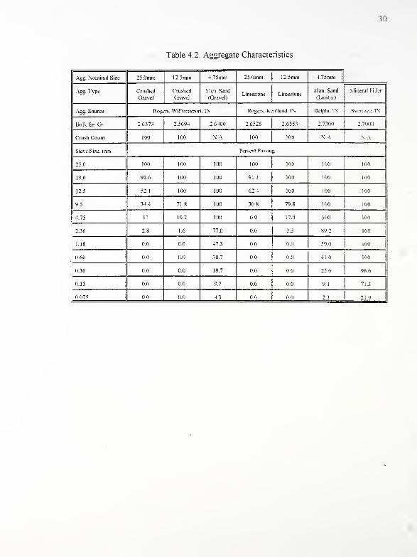
specifications. Table 4.2 lists aggregate characteristics and sources Each aggregate
source is INDOT approved.
4.2.2 Asphalt Mixtures
Four asphalt mixtures were studied. These included #1 1 surface mixes, 12.5 mm
nominal maximum aggregate size, and #8 binder mixes, 25.0 mm nominal maximum
aggregate size as defined by INDOT. Two aggregate types, limestone and gravel
aggregate, were utilized. INDOT aggregate specifications require 100 percent of the
24
particles have one crushed face for high volume surface mixes and a minimum of 95
percent for high volume binder mixes (INDOT, 1995) INDOT also restricts the type of
aggregate to slag or limestone.
Mix designs were conducted using a 75 blow Marshall hand-hammer compaction
effort Optimum asphalt contents were selected solely on 6 percent air voids which is
INDOT' s criteria. Otherwise, the mix design followed the procedure described in the
Asphalt Institute Manual, MS-2 (Asphalt Institute, 1995). INDOT mix design criteria
includes a minimum stability of 5340 N, and a maximum flow value of 16. Voids in the
mineral aggregate requirements are a minimum of 16.0% and 14.0% for the surface and
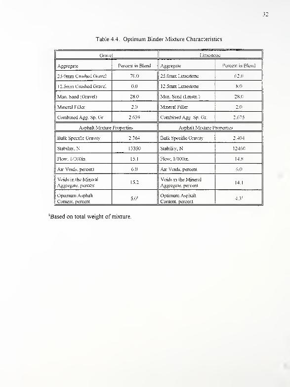
the binder mixes, respectively. Characteristics of the surface and binder mixes are listed
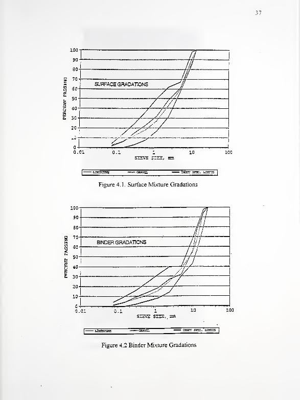
in Tables 4.3 and 4.4, respectively. The gradations for the surface mixtures are shown in
Figure 4 1 and those for the binder mixtures in Figure 4.2.
4.3 Laboratory Segregation Techniques
Five mixes with varying degrees of segregation were produced for each of the
four HMA types. The mixtures designated as the control mix were the result of the
Marshall mixture design method outlined in Table 4.3 and Table 4.4. These mixtures
were included in the study as one of the five degrees of segregation.
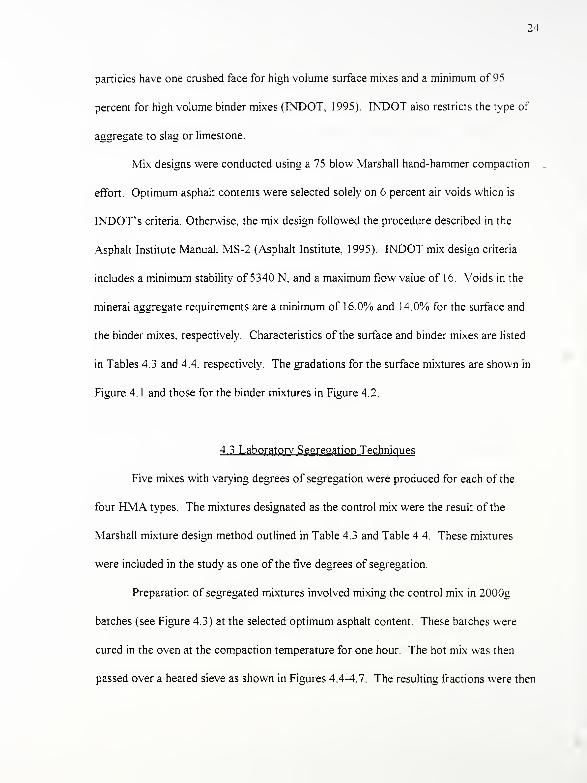
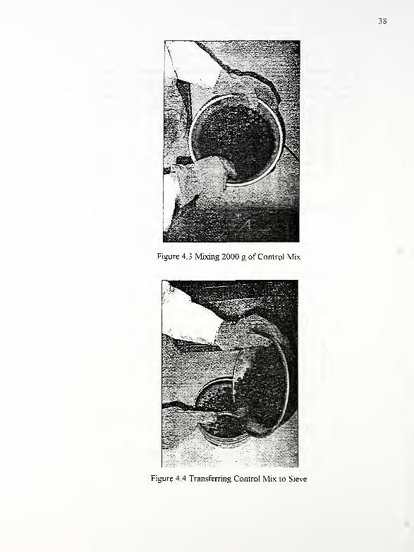
Preparation of segregated mixtures involved mixing the control mix in 2000g
batches (see Figure 4.3) at the selected optimum asphalt content These batches were
cured in the oven at the compaction temperature for one hour The hot mix was then
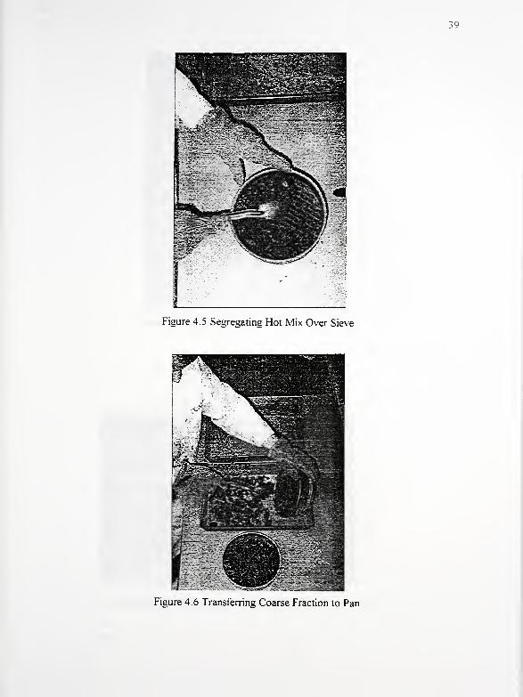
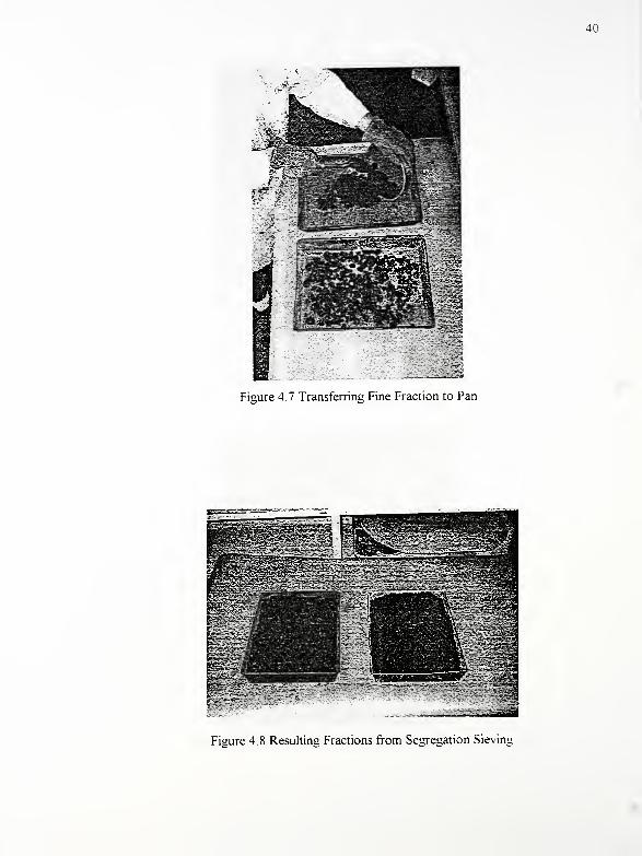
passed over a heated sieve as shown in Figures 4.4-4.7. The resulting fractions were then
25
placed into pans for further material testing.
The sieves were selected based on the fact that when the heated control mix was
passed through the sieve, approximately 50% was retained and 50% passed These
proportions made estimation of material quantities easier. Enough material for each mix
was prepared in 2000g batches to provide adequate amounts of segregated material to
conduct the asphalt extraction tests and subsequent gradation analysis. This sieving
created two fractions of the control mix (refer to Figure 4.8), coarse (retained on the
sieve) and fine (passing the sieve). These fractions were used as two degrees of
segregation, very coarse and very fine.
Two other mixes were produced with intermediate degrees of segregation by
combining differing percentages of the coarse and fine materials. The five mixtures were
produced using the percentages of coarse and fine material outlined in Tables 4.5 and 4 6
Bryant (1968) developed these manual segregation procedures using laboratory
prepared surface mixtures. In the study, a procedure was developed to pass fresh hot mix
over heated sieves and proportion the resulting fractions to examine varying asphalt
content and film thickness with different gradations. This "segregation" was quantified
based on gradation and extracted asphalt content. Khedaywi and White ( 1 994) used a
similar laboratory procedure to develop the segregated proportions for an Indiana #8
Binder and #1 1 Surface mixtures.
4.4 Characterization of Segregated Mixtures
Physical properties of laboratory segregated and compacted asphalt mixtures were

26
determined. These properties established the baseline for measurements with the
proposed nondestructive testing equipment. These physical properties included asphalt
content, gradation, density and voids.
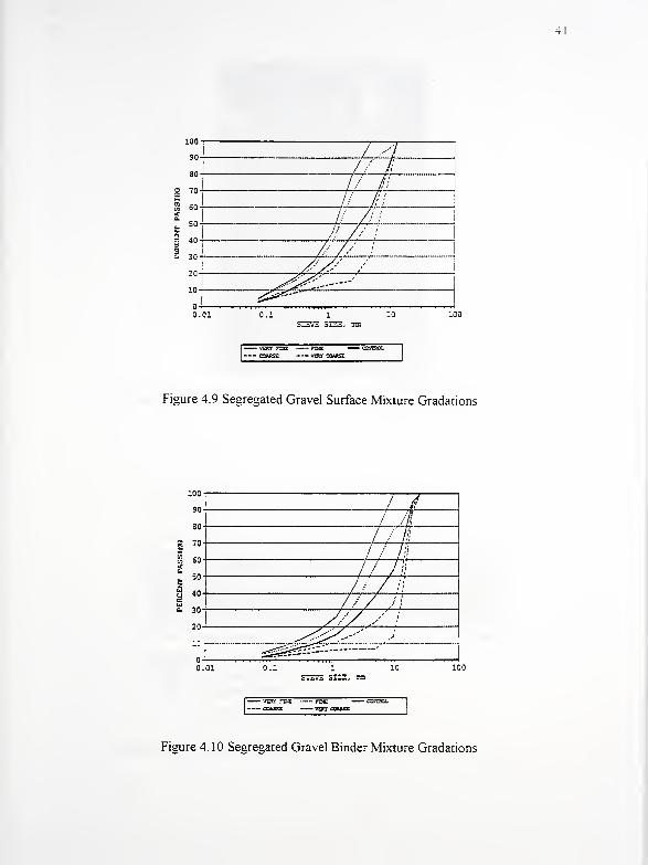
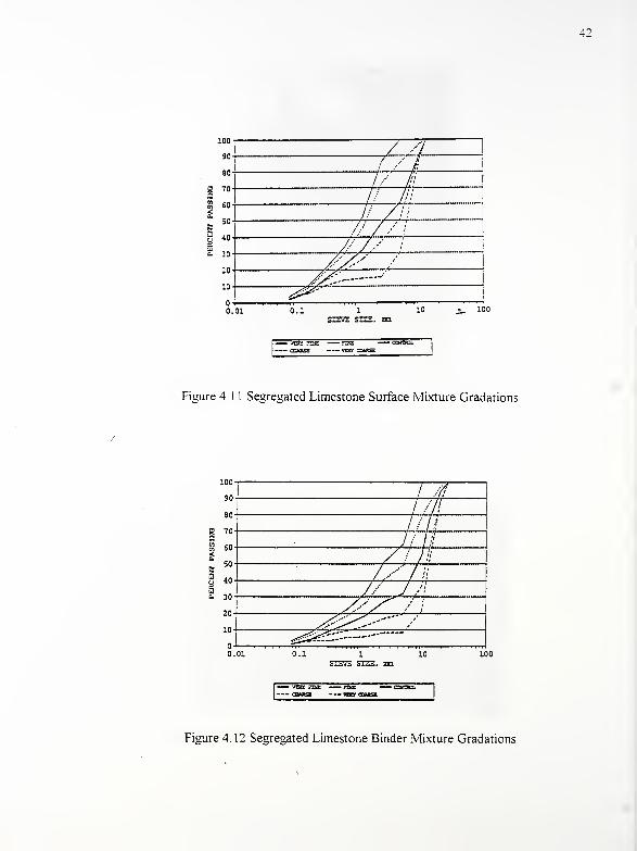
4.4.1 Segregated Mixture Asphalt Content/Gradation
Extractions (ASTM D 2172 - 92) and sieve analyses (ASTM C 136) were
performed on each mixture prepared at the five levels of segregation. Results of the
extractions are shown in Table 4.7. The gradations of the segregated limestone #1
1
surface and #8 binder mixtures are shown in Figures 4.9 and 4. 10, respectively.
Corresponding gradations of the segregated gravel mixtures are shown in Figures 4. 1
1
and 4.12, respectively. The specific asphalt content and gradation for each level of
segregation were used in preparing batches of mixtures for testing.
4.4.2 Density and Air Voids
A target density was required for each segregated mixture to prepare samples for
testing. In attempts to compact segregated mixtures with the Marshall hand-hammer, the
very coarse mixtures exhibited considerable aggregate crushing and the very fine mixture
flushed. In the latter case, material flowed up the sides of the Marshall mold and collar
during compaction. As an alternative, samples were compacted in the Gyratory Testing
Machine (GTM) using procedures in ASTM D 3387-83.
GTM compaction conditions were 1380 kPa vertical pressure, 1 degree angle of
gyration and 30 revolutions. Four samples were prepared for each level of segregation
27
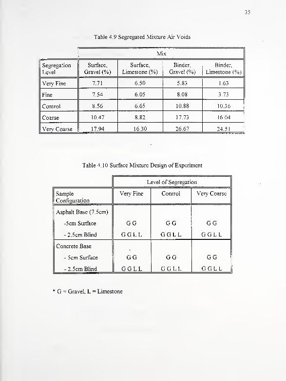
Resulting density and air voids based on the GTM compacted samples are given in
Tables 4.8 and 4.9, respectively.
4.5 Laboratory Specimens for Non-Destructive Testing
Planned non-destructive tests of the segregated mixtures required that compacted
samples be large enough so that the results would not be influenced by sample size In
order that samples meet the size criteria, a linear compactor was designed and fabricated
(Brown, K. 1993). The non-destructive tests that were planned included thermal
imaging, air permeability, nuclear moisture(asphalt) and density, and permittivity
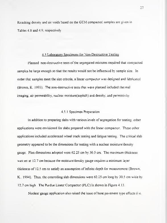
4.5. 1 Specimen Preparation
In addition to preparing slabs with various levels of segregation for testing, other
applications were envisioned for slabs prepared with the linear compactor. These other
applications included accelerated wheel track testing and fatigue testing. The critical slab
geometry appeared to be the dimensions for testing with a nuclear moisture/density
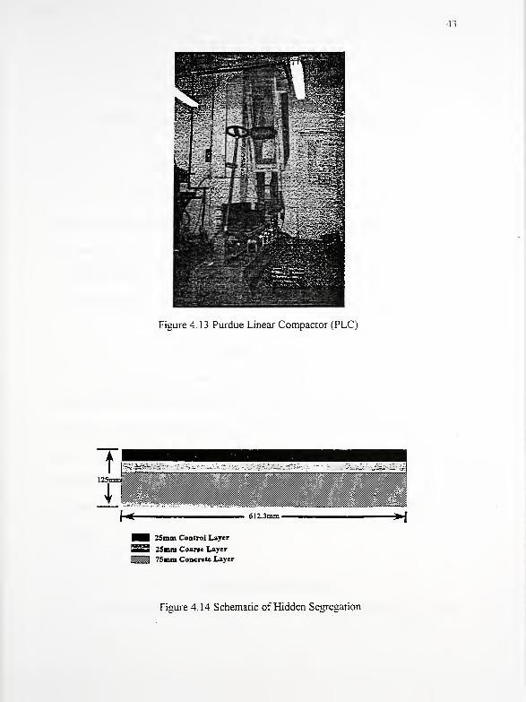
gauge. Plan dimensions adopted were 62.25 cm by 30.5 cm. The maximum thickness
was set at 12.7 cm because the moisture/density gauge requires a minimum layer
thickness of 12.5 cm to satisfy an assumption of infinite depth for measurement (Brown.
K., 1994). Thus, the controlling slab dimensions were 62.25 cm long by 30.5 cm wide by
12.7 cm high. The Purdue Linear Compactor (PLC) is shown in Figure 4.13.
Nuclear gauge application also raised the issue of base pavement type effects (i.e.
28
asphalt or concrete). Consequently, both types of base layers were incorporated into the
tests. In taking this approach, slabs were prepared that would represent the cases of a
thin overlay of an asphalt or concrete base. An overlay thickness of 5 1 cm and a base
thickness of 7.6 cm were adopted. The asphalt base (control mixture) was prepared at the
same time as the segregated overlays. Concrete bases were fabricated in advance They
were allowed to cure for a minimum of 21 days before applying a tack coat and
compacting the hot mix asphalt on top.
Two segregated conditions were considered, hidden segregation and visible,
surface segregation. Figure 4.14 shows a schematic of samples prepared with hidden
segregation. Tables 4. 1 and 4. 1 1 show the tests that have been conducted. Factors
tested were mix type, aggregate type, control and extreme segregation, and hidden (blind)
and visible, surface segregation.
Material for each 2.5 cm of compacted slab was batched and mixed in a Hobart
mixer. These batches were placed in a forced draft oven for an hour to allow for asphalt
absorption. Mixtures prepared at each level of segregation were compacted in the PLC to
the previously determined GTM densities for each level of segregation.
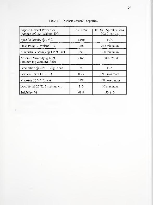
Table 4. 1 . Asphalt Cement Properties
29
Asphalt Cement Properties
(Amoco AC-20, Whiting, IN)
Test Result INDOT Specifications,
902 01(g)-93.
Specific Gravity @ 25 °C 1.036 N/A
Flash Point (Cleveland), °C 288 232 minimum
Kinematic Viscosity @ 135°C, cSt 393 300 minimum
Absolute Viscosity @ 60°C
(300mm Hg vacuum), Poise
2165 1600-2500
Penetration @ 25 °C, lOOg, 5 sec 65 N/A
Loss on Heat (T.F.O.T.) 0.25 99.0 minimum
Viscosity @ 60°C, Poise 5293 8000 maximum
Ductility @ 25 °C, 5 cm/min, cm 110 40 minimum
Solubility, % 99.9 50-110
30
Agg. Nominal Size; 25.0iiiiii 12.5mm 4.75mm 25.0mm 1 2.5mm 4.75mni
Agg. Type Crushed
Gravel
Crushed
Gravel
Man. Sand
(Gravel)Limestone Limestone
Man. Sand
(Lmstn)
Mineral Filler
Agg- Source Rogers. Williamsport. IN Rogers. Kenlland. IN Delphi. IN Suav/ec. IN
Bulk Sp. Gr. 2.6373 2.5694 2.6400 2.6526 2.6553 2.7300 2.7000
Crush Count 100 100 N A 100 100 \ A N A
Sieve Size, nun Percent Passing
25.0 100 100 100 100 100 100 100
19.0 92.6 100 100 91.1 100 100 100
12.5 52.1 100 100 62.4 100 100 100
9.5 34.4 71.8 100 30.8 79.8 100 100
4.75 11 10.2 100 0.9 17.0 100 100
2.36 2.8 1.6 770 0.0 1.5 89.2 100
1.18 0.0 0.0 47.3 0.0 0.0 59.0 100
0.60 0.0 0.0 30.7 0.0 0.0 41.0 100
0.30 0.0 0.0 19.7 0.0 0.0 25.6 96.6
0.15 0.0 0.0 9.7 0.0 0.0 9.1 71.3
075 0.0 0.0 4.3 0.0 0.0 2.1 21.9
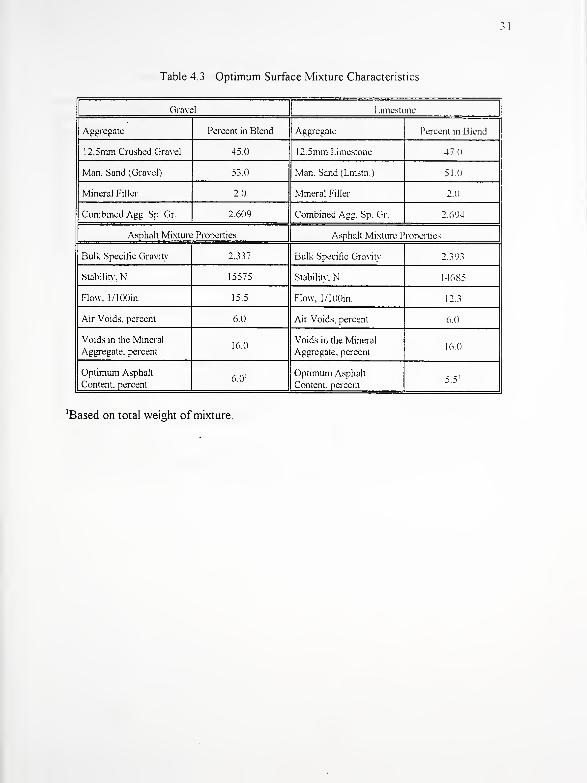
Table 4.3. Optimum Surface Mixture Characteristics
Grave] Limestone
Aggregate Percent in Blend Aggregate Percent in Blend
12.5mm Crushed Gravel 45.0 12.5mm Limestone 47.0
Man. Sand (Gravel) 53.0 Man. Sand(Lmstn.) 51.0
Mineral Filler 2.0 Mineral Filler 2.0
Combined Agg. Sp. Gr. 2.609 Combined Agg. Sp. Gr. 2.694
Asphalt Mixture Properties Asphalt Mixture Properties
Bulk Specific Gravity 2.337 Bulk Specific Gravity 2.393
Stability, N 15575 Stability, N 1 4685
Flow. l/100in. 15.5 Flow. 1/lOOin 12.3
Air Voids, percent 6.0 Air Voids, percent 6.0
Voids in the Mineral
Aggregate, percent16.0
Voids in the Mineral
Aggregate, percent16.0
Optimum Asphalt
Content, percent6.0'
Optimum Asphalt
Content, percent5.5
1
'Based on total weight of mixture.
32
Table 4.4. Optimum Binder Mixture Characteristics
Gravel Limestone
Aggregate Percent in Blend Aggregate Percent in Blend
25.0mm Crushed Gravel 70.0 25.0mm Limestone 62.0
1 2.5mm Crushed Gravel 0.0 12.5mm Limestone 8
Man. Sand (Gravel) 28.0 Man. Sand (Lmstn.) 28.0
Mineral Filler 2.0 Mineral Filler 2.0
Combined Agg. Sp. Gr. 2.639 Combined Agg. Sp. Gr. 2.675
Asphalt Mixture Properties Asphalt Mixture Properties
Bulk Specific Gravity 2.364 Bulk Specific Gravity 2 404
Stability, N 13350 Stability. N 1 2460
Flow. 1/luOin. 15.1 Flow, 1/1 00m. 14.8
Air Voids, percent 6.0 Air Voids, percent 6.0
Voids in the Mineral
Aggregate, percent15.2
Voids in the Mineral
Aggregate, percent14.1
Optimum Asphalt
Content, percent5.0'
Optimum Asphalt
Content, percent4.3
1
"Based on total wei«ht of mixture.
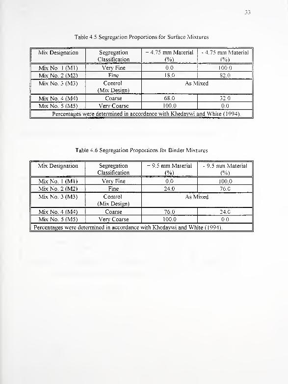
Table 4.5 Segregation Proportions for Surface Mixtures
Mix Designation Segregation
Classification
+ 4.75 mm Material
(%)
- 4.75 mm Material
(%)
Mix No 1 (Ml) Verv Fine 0.0 1000
Mix No. 2 (M2) Fine 18.0 820
Mix No. 3 (M3) Control
(Mix Design)
As Mixed
Mix No. 4 (M4) Coarse 68.0 32.0
Mix No. 5 (M5) Very Coarse 100.0 0.0
Percentages were determined in accordance with Khedaywi and White ( 1994)
Table 4.6 Segregation Proportions for Binder Mixtures
Mix Designation Segregation
Classification
+ 9.5 mm Material
(%)
- 9.5 mm Material
(%)
Mix No. 1 (Ml) Verv Fine 0.0 100.0
Mix No. 2 (M2) Fine 24.0 76.0
Mix No. 3 (M3) Control
(Mix Design)
As Mixed
Mix No. 4 (M4) Coarse 76.0 24.0
Mix No. 5 (M5) Very Coarse 100.0 0.0
Percentages were determined in accordance with Khedaywi and White (1994)
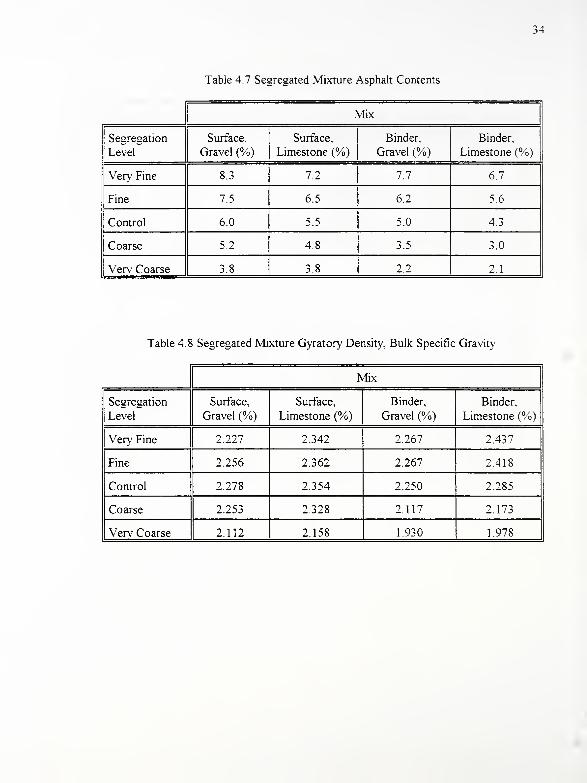
Table 4.7 Segregated Mixture Asphalt Contents
Mix
Segregation
Level
Surface,
Gravel (%)
Surface,
Limestone (%)
Binder,
Gravel (%)
Binder,
Limestone (%)
Very Fine 8.3 7.2 7.7 6.7
Fine 7.5 6.5 6.2 5.6
Control 6.0 5.5 5.0 4.3
Coarse 5.2 4.8 3.5 3.0
Very Coarse 3.8 3.8 2 2 2.1
Table 4.8 Segregated Mixture Gyratory Density, Bulk Specific Gravity
Mix
Segregation
Level
Surface,
Gravel (%)
Surface,
Limestone (%)
Binder,
Gravel (%)
Binder,
Limestone (%)
Very Fine 2.227 2.342 2.267 2.437
Fine 2.256 2.362 2.267 2.418
Control 2.278 2.354 2.250 2.285
Coarse 2.253 2.328 2.117 2.173
Very Coarse 2.112 2.158 1.930 1.978
Mix
Segregation
Level
Surface,
Gravel (%)
Surface,
Limestone (%)
Binder,
Gravel (%)
Binder,
Limestone (%)
Very Fine 7.71 6.50 5.83 1.63
Fine 7.54 6.05 8.08 3.73
Control 8.56 6.65 10.88 10.36
Coarse 10.47 8.82 17.73 16.04
Verv Coarse 17.94 16.30 26.67 24.51
Table 4.10 Surface Mixture Design of Experiment
Level of Segregation
Sample Very Fine Control Very Coarse
Configuration
Asphalt Base (7.5cm)
-5cm Surface GG GG GG
-2.5cm Blind GGLL GGLL GGLL
Concrete Base
- 5cm Surface GG GG GG
-2.5cm Blind GGLL GGLL GGLL
* G = Gravel, L = Limestone
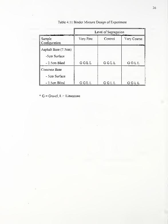
Table 4. 1 1 Binder Mixture Design of Experiment
Level of Segregation
Sample
Configuration
Very Fine Control Very Coarse
Asphalt Base (7.5cm)
-5cm Surface
-2.5cm Blind GGLL GGLL GGLL
Concrete Base
- 5cm Surface
- 2.5cm Blind GGLL GGLL GGLL
G = Gravel, L = Limestone
100
SIEVE SIZE, nm
2BOT 3?SC.
Figure 4.1. Surface Mixture Gradations
100
90
80
§ 70
I 50<Oi
SO
g 40IT
£ 30
20
10
//_/[:/
\ BINDEH GRADATIONS /w/ *7
_J/jI / .^/ z^yj ^^^
y
i^<^-^
0.01 0.1 10
sieve SIZE, am100
' 21DCT a?£E. L2CTS
Figure 4.2 Binder Mixture Gradations
38
Figure 4.3 Mixing 2000 g of Control Mix
Figure 4.4 Transferring Control Mix to Sieve
39
Figure 4.5 Segregating Hot Mix Over Sieve
Figure 4.6 Transferring Coarse Fraction to Pan
40
Figure 4.7 Transferring Fine Fraction to Pan
Figure 4.8 Resulting Fractions from Segregation Sieving
41
SIEVE SIZE, mm
Figure 4.9 Segregated Gravel Surface Mixture Gradations
SIEVE SXSS, an
Figure 4.10 Segregated Gravel Binder Mixture Gradations
42
vnce =aues:
Figure 4.11 Segregated Limestone Surface Mixture Gradations
SIEVE SIZE, am
Figure 4.12 Segregated Limestone Binder Mixture Gradations
43
Figure 4. 1 3 Purdue Linear Compactor (PLC)
25mm Control Layer
25mm Coarse Layer
75mm Concrete Layer
Figure 4.14 Schematic of tiidden Segregation
44
CHAPTER 5. NON-DESTRUCTIVE TESTING FOR SEGREGATION
5.1 Introduction
One objective of this study was to identify technologies for detecting segregation
Detection implies that one or a combination of physical characteristics could be measured
and subsequently correlated with degree of segregation. Technologies considered were:
1 . thermal imaging, 2. air/water permeability, 3. nuclear moisture(asphalt) and density,
and 4. permittivity.
Thermal imaging equipment was field tested on an existing pavement, at a hot
mix asphalt plant, and at a paving project to determine its overall effectiveness in
detecting segregation. The basis for using this equipment was that different size
aggregates would retain or gain heat at different rates. In general, thermal imaging did
confirm locations of segregated areas that were visually identified. However, the
technology was not considered effective in locating segregation occurring beneath the
surface.
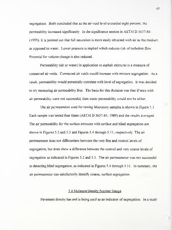
5.3 Water or Air Permeability
Zube (1962) and Brown, et al (1989) conducted water permeability tests to detect
45
segregation. Both concluded that as the air void level exceeded eight percent, the
permeability increased significantly. In the significance section in ASTM D 3637-84
(1995), it is pointed out that full saturation is more easily obtained with air as the medium
as opposed to water. Lower pressure is implied which reduces risk of turbulent flow.
Potential for volume change is also reduced.
Permeability (air or water) in application to asphalt mixtures is a measure of
connected air voids. Connected air voids would increase with mixture segregation As a
result, permeability would potentially correlate with level of segregation. It was decided
to try measuring air permeability first. The basis for this decision was that if tests with
air permeability were not successful, then water permeability would not be either.
The air permeameter used for testing laboratory samples is shown in Figure 5.1
Each sample was tested four times (ASTM D 3637-84, 1989) and the results averaged.
The air permeability for the surface mixtures with surface and blind segregation are
shown in Figures 5.2 and 5.3 and Figures 5.4 through 5.11, respectively. The air
permeameter does not differentiate between the very fine and control levels of
segregation, but does show a difference between the control and very coarse levels of
segregation as indicated in Figures 5.2 and 5.3. The air permeameter was not successful
in detecting blind segregation, as indicated in Figures 5.4 through 5.11. In summary, the
air permeameter can satisfactorily identify coarse, surface segregation.
5.4 Moisture/Density Nuclear Gauge
Pavement density has and is being used as an indicator of segregation In a study

46
for the Georgia DOT (Brown et al, 1989) used nuclear density to indicate segregation as
part of construction quality control. Cross and Brown (1993) used a thin lift nuclear
gauge to measure densities in areas visually identified as segregated.
Careful consideration of the principles on which the nuclear gauge operates
suggests that the nuclear moisture/density gauge can be used to measure asphalt content
The moisture reading is independent of the density measurement as there are two
different sources, and thus the measurements are not correlated with each other (Troxier.
1993). When moisture measurements are made, the "count" depends on the heavy
hydrogen atoms. Asphalt is a hydrocarbon material and therefore the asphalt hydrogen
atoms could be "counted" by the nuclear gauge. It is also recognized that the pavement
would have to be in a dry condition for the asphalt content reading.
Consequently, tests were conducted using the nuclear gauge to measure both
density and asphalt (moisture) content of laboratory compacted slabs prepared with
different levels and location of segregation. The nuclear moisture/density gauge and a
test slab are shown in Figure 5.12.
5.4.1 Calibration
Nuclear density calibration is conducted using blocks of three different materials.
These blocks consist of magnesium, aluminum and a laminated aluminum and
magnesium. The aluminum and magnesium blocks represent two extremes in density,
1 1 and 1 70 pcf, respectively. A midpoint density is achieved with the laminated block
of aluminum and magnesium.
47
Two blocks are used for moisture content calibration, magnesium and
polyethylene. The magnesium block represents zero moisture content and the
polyethylene block represents an infinite volume of water because of the high number of
hydrogen atoms. The gauge calibration is a straight line between these two extremes
Four minute counts are used for calibrating the gauges (K. Brown, 1995).
A standard count should be taken before use to check gauge operation and allow
for source decay (Troxler, 1988). For the particular gauge used in this study, the gauge
automatically compares the new count to the average of the last four standard counts.
The new count will "pass1' if it is within two percent of the moisture average and/or one
percent of the density average of the previous four counts. The Manual of Operation and
Instruction (Troxler, 1988) should be consulted to ensure safe operating procedures.
5.4.2 Moisture (Asphalt) Content and Density
For this study, the gauge was operated in the soils backscatter modes. The gauge
contains two radioactive sources. Cesium-137 is used to measure density and is located
within a rod on the left side of the gauge. Americium-24 1 :Beryllium is used for moisture
measurement and is located inside the gauge near the center of the base.
5.4.3 Test Procedure Discussion
The number of readings taken with the nuclear gauge was four one minute
readings. Belt et al., (1991), concluded that a minimum of four density readings taken for
each density measurement and averaged provided very good to excellent final density
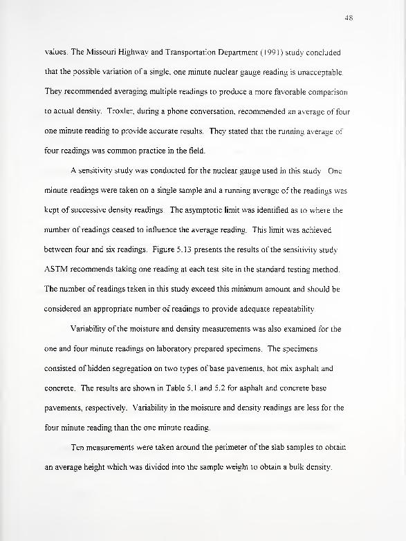
48
values. The Missouri Highway and Transportation Department ( 1991 ) study concluded
that the possible variation of a single, one minute nuclear gauge reading is unacceptable
They recommended averaging multiple readings to produce a more favorable comparison
to actual density. Troxler, during a phone conversation, recommended an average of four
one minute reading to provide accurate results. They stated that the running average of
four readings was common practice in the field.
A sensitivity study was conducted for the nuclear gauge used in this study. One
minute readings were taken on a single sample and a running average of the readings was
kept of successive density readings. The asymptotic limit was identified as to where the
number of readings ceased to influence the average reading This limit was achieved
between four and six readings. Figure 5.13 presents the results of the sensitivity studv
ASTM recommends taking one reading at each test site in the standard testing method
The number of readings taken in this study exceed this minimum amount and should be
considered an appropriate number of readings to provide adequate repeatability
Variability of the moisture and density measurements was also examined for the
one and four minute readings on laboratory prepared specimens. The specimens
consisted of hidden segregation on two types of base pavements, hot mix asphalt and
concrete. The results are shown in Table 5.1 and 5.2 for asphalt and concrete base
pavements, respectively. Variability in the moisture and density readings are less for the
four minute reading than the one minute reading.
Ten measurements were taken around the perimeter of the slab samples to obtain
an average height which was divided into the sample weight to obtain a bulk density.
49
Habermann (1994) used this procedure to obtain the bulk density of the slabs he
fabricated with the PLC.
The measured density was used to produce a basis for comparison to establish
appropriate correction factors based on the material properties and sample configurations.
These measured densities were used as the basis for density correction factors.
This data also provided a means to measure the effectiveness of the PLC in
compaction ofHMA. The control mix, full depth slabs could be used in this analysis,
assuming uniform compaction throughout the depth of the sample. The segregated
samples prevented an estimate of percent compaction obtained with the PLC due to the
fact that the density was not uniform throughout the sample (as is the case also with the
concrete base slabs ). The percent compaction obtained with the PLC when comparing
measured densities to target densities from Table 4.8 averaged 96.1 percent compaction
given in Table 5.3. The results show that the PLC is an effective compaction device that
can produce compactive efforts equivalent to those experienced in the field
5.4.4 Correction Factors
ASTM D 2950-91 states that it is necessary to establish a density correction factor
based on each project. Belt et.al, (1991) also recommended the establishment of density
correction factors for each paving project. Kennedy et.al, ( 1 989) stated that density
calibration factors are necessary for each project to provide acceptable results
ASTM D 4125-83 recommends the development of a calibration curve for
correction of nuclear asphalt contents. Regan (1975) recommended the establishment of
50
a nuclear calibration curve over a range of asphalt contents
Belt et al., (1991) stated that variations in the nuclear gauge density results can be
reduced by utilizing user provided inputs. He stated that these variations are caused by
variables that are inherent in the pavement mat. The variables that could affect nuclear
gauge readings include chemical composition of the material being tested, size and
geometry of the aggregate and density variations in the asphalt mix
A bias analysis was conducted of the nuclear moisture/density gauge results to
identify the need for establishment of correction factors for the results of this study. This
analysis served to identify any bias caused by main level effects. Main level effects are
those independent factors that were varied as a part of this study These factors include
mixture type, base pavement and degree of segregation The analysis was conducted by
plotting the nuclear gauge results against the known material properties which were used
as the basis for establishing correction factors. Figures 5. 14 - 5.21 contain the plots of
this analysis.
In the analysis, a "least squares" linear regression was performed on the data for
each mix type and compared to the "optimum fit line". The optimum fit line is the line
that represents perfect accuracy between nuclear gauge readings and the known material
properties used for calibration.
The nuclear gauge density readings for the #1 1 Surface and #8 Binder mixtures,
presented in Figures 5.14 and 5.16, show little or no bias from degree of segregation or
base pavement. The results suggest that these mixes would require no density calibration
for these main level effects.
51
The nuclear density readings for the #1 1 Limestone and #8 Limestone, presented
in Figures 5.15 and 5.17, do show bias from either degree of segregation or base
pavement. As a result, the bias analysis on these mixes was extended to also analyze the
bias effect due to differing base pavements. The resulting regression lines show a
distinct bias caused by base pavement on the limestone mixes. The main level effects on
the limestone mix density results are discussed further in Section 5.4.5.
When comparing the gravel mixes to the limestone mixes, it is apparent that there
could be a bias caused by aggregate type. The limestone mixes exhibit a large disparity
between nuclear gauge results and the known densities when compared to the gravel
mixes. The plots also show that the nuclear gauge overpredicts density for both
limestone mixes, regardless of base pavement. This bias is not unexpected based on
factory calibration of the nuclear gauge as discussed in Section 5.4.5.
The bias analysis plots for nuclear asphalt content based on each mix are
presented in Figures 5.18- 5.21. The bias analysis of the nuclear asphalt contents allows
statements to be made concerning the effect degree of segregation has on the results.
Degree of segregation in this study is marked by controlled variations in the as-mixed
asphalt content. The data groupings in all of the asphalt content bias plots inherently
show the levels of segregation for each mix type. If the regression lines are not parallel
with the optimum fit lines, one could state that these biases are caused by variations in
the asphalt percentage due to degree of segregation.
The bias analysis for each mix was extended to confirm any bias effects due to
base pavement. The results of the extended analysis show that the regression lines divide

52
the data into two distinct groups. These groups are defined as having either asphalt or
concrete bases.
By comparing the nuclear asphalt content bias plots of all of the mixes, one can
state that bias is caused by both aggregate type, mix type, base pavement and degree of
segregation. One may also state that the nuclear gauge overpredicts asphalt content All
of the bias statements concerning nuclear asphalt content are further discussed in Section
5.4.6.
By correcting for the main level effects identified in the bias analysis, it may be
possible to minimize their effect on the nuclear gauges precision This correction may
also reduce the apparent variability of the nuclear gauge results. Consequently, the
gauges may then be utilized to generate data which could be used to accurately classify
the results into degree of segregation.
The common practice for the establishment of density correction factors is to take
nuclear density readings on a pavement and correlate those readings with cores taken
from each of the testing locations. Correction for asphalt content readings can be
obtained by correlation between readings and extracted asphalt percentages. Since this
study was conducted in the laboratory, the known material properties were used as the
basis for the correction factors. The process followed in this study for establishing
correction factors was as follows:
1
.
Take four, one minute readings on each sample and or test site
2. Average the four readings.
3. Compare average readings to known material properties.
^J
4. Establish correction factor for each sample and or test site.
5 Analyze the correction factors based upon the independent factors of the
study, which include, aggregate and mix type, degree of segregation and
base pavement.
6. Establish a standard correction factor based on each of these independent
factors at a 95% confidence interval.
The correction factors used in this study for density and asphalt contents are given
in Tables 5.4 and 5.5. These correction factors were established based on the process
discussed in Appendix C. The analysis of the correction factors based on the
independent factors of the study is discussed in sections 5.4.5 and 5.4.6. The output of
the analysis concerning the independent factors of the study is contained in Appendix C.
5.4.5 Nuclear Density
The bias analysis conducted in Section 5.2.3 served to identify potential main
level effects that could result in erroneous nuclear density readings. The correction
factors established for nuclear density in this study were analyzed statistically to further
identify and understand the independent variables to which the nuclear gauge were most
sensitive. Establishment of these correction factors is critical to accounting for the
variations inherent in the gauges sensitivity to certain properties of the materials being
tested. By addressing these variations through correction factors, their effect in the
classification process could be eliminated. As a result, the possibility of misclassification
54
based on erroneous readings due to the effect of material properties could be reduced
Independent variables in the analysis were Degree of Segregation (DOS), Mixture
Type (MIXTYPE) and Base Pavement (BSEPAV), each having 3, 4, and 2 levels
respectively. The dependent variable was nuclear density.
The General Linear Models (GLM) procedure used in SAS was used for the
correction factor analysis. Output from the GLM analysis of the nuclear density
correction factors is presented in Appendix C. The analysis indicated that DOS had no
effect on the nuclear gauge readings for density. This finding is positive since DOS will
not be able to be preestablished in the field. The analysis also showed that BSEPAV and
MIXTYPE were significant to the GLM model. These will be either be known or can be
tested for to preestablish correction factors for field application of this method.
The MIXTYPE variable included both asphalt mixture types (#1 1 Surface and #8
Binder) and aggregate types (Gravel and Limestone). It is expected that MIXTYPE
would be significant based on how the nuclear gauge is calibrated in the factory.
The density calibration method used at the factory consists of the accumulation of
count rate data on five standard density blocks and then on a standard density block to
verify calibration accuracy. The accumulation of data on the various calibration blocks
provides count rate results for varied densities. These results can then be used in
computations of density versus count rate to establish a calibration for a wide range of
densities (Troxler Users Manual). Of the five calibration blocks, two are non-metallic
and are used for the soil calibration. The two standard blocks are granite and limestone
The assumption is that the density of most soils will fall between the density of these two
ss
limits. So, a calibration with these two materials as the limits will provide a calibration
suitable for all normal soils. The other three standard density blocks are metallic and are
used to provide data for other factors in Troxler's calibration model (Troxler Users
Manual).
By acknowledging this calibration process, one can expect that MIXTYPE would
be a significant factor since one of the aggregates in the study is limestone and is on the
outside range of the gauge calibration. In a phone conversation with Troxler, they agreed
that the limestone mixes would require larger correction factors and be significant due to
the factory calibration. The calibration places limestone on the lower limit, meaning it
has a lower count rate. This lower count rate would result in a higher density reading, as
the results show. The correction factor required lowers the density reading, meaning the
gauge overpredicted the density on the limestone samples.
Table 5.4 presents a finding concerning MIXTYPE and its two components,
mixture and aggregate type. It can be seen that aggregate type had a larger effect on the
nuclear gauge density readings than mixture type. The gravel and limestone mixtures
required different correction factors, but the #1 1 Surface to #8 Binder comparison
showed similar correction factors for each aggregate type.
The GLM analysis also concluded that BSEPAV was a significant factor to the
density model at a 95% confidence interval. This sensitivity to base pavement was found
to be true only for the limestone mixes.
It should be noted that the varied results due to the two base pavements may not
be totally attributable to the fact that the samples had different base materials. Effects

56
due to the thickness of the asphalt layer, although not clearly identified in this study.
could prove to be a factor in the gauges precision. The differing base samples in the study
had different depths of compacted asphalt. The concrete base samples had a two inch
asphalt lift, while the full depth asphalt slabs had a five inch asphalt lift These different
thicknesses of the asphalt layer could be found to have an effect on the gauge readings
Table 5.4 outlines the density correction factors used for the samples in this study
Figures 5.22 to 5.29 show the plots of the corrected density readings for both asphalt and
concrete base samples. The figures show that the nuclear gauge was effective in
detecting the density trend for segregated mixtures, which decreases from fine to coarse
mixtures. The results also agree with the results of the Cross and Brown study ( 1 993)
which concluded that coarsely segregated areas will have lower unit weight values when
measured with the nuclear gauge.
The results also show that, in general, the segregated sample density results fell
below the 95% minimum density line required by INDOT in field compaction These
low density samples with segregated areas would be unacceptable since they are below
the minimum acceptable density. The results show that the nuclear gauge is effective in
identifying density variations that would be unacceptable from a quality control
standpoint.
5.4.6 Nuclear Asphalt Content Discussion
The bias analysis conducted in Section 5.4.4 served to identify potential main
level effects that could result in erroneous nuclear asphalt content readings. Correction
57
factors established for nuclear asphalt content results in this study were analyzed
statistically using the SAS GLM procedure. The GLM analysis identified independent
variables suspected of having the largest effect on the nuclear gauge readings of asphalt
content. The GLM analysis also served to further understand the main level effects that
were causing any identified bias. Output from the GLM analysis of the nuclear asphalt
content correction factors is presented in Appendix C.
Independent variables were DOS, MIXTYPE and BSEPAV, The dependent
variable was asphalt content. DOS, MIXTYPE and BSEPAV were all found to be
significant to the GLM model for the nuclear gauge asphalt readings This finding shows
that the nuclear gauge readings are very sensitive to physical property variations in the
mix when it is used to determine asphalt content. ASTM D 4125-83 states that the
asphalt content reading is sensitive to aggregate type, source and percentage of asphalt
and mix gradation. The standard supports the findings of the GLM analysis and
recommends the establishment of correction curves based on the resulting asphalt
percentages obtained for each job mix.
Even though the analysis showed that the asphalt content correction factors varied
with base pavement, it should be noted that these varied results may not be totally
attributable to the fact that the samples had different base materials. The different
thicknesses of the asphalt layers in this study may have an effect on the asphalt content
readings.
A significant finding of the analysis was that the asphalt correction factors were
affected by DOS. Since the asphalt content results varied based on DOS. it can be stated
58
that the nuclear gauge moisture reading is sensitive to the amount of asphalt in the mix
This statement is supported by ASTM D 4125-83.
This finding is significant since DOS is the only factor in this study that can not
be accounted for in the field. If it was determined that the nuclear gauge was sensitive to
DOS for certain mixes, it would be necessary to correct for this factor, since DOS will be
unknown in the field. MIXTYPE and BASEPAV would be preestablished based on the
job mix and job conditions.
Trends from the corrected asphalt content readings match well with the trends
obtained through extractions run on very coarse and very fine segregated mixes, which
are presented in Figure 5.30. Even though the segregated layer is being tested along with
a uniform layer, the segregation effect on asphalt content variation is still evident through
the corrected readings.
Table 5.5 shows the correction factors used in this study for each of the various
samples. The correction factors vary more than the density factors since the asphalt
content test is more sensitive to material properties. Figures 5.31 To 5.38 show the
corrected nuclear asphalt content readings for each of the sample configurations. The
figures also show that the fine and coarse segregated sample readings are out of the
acceptable range for asphalt percentage variation.
Kandhal et al., (1978) stated that the presence of absorbed moisture in the
aggregate can cause problems in nuclear gauge readings since the hydrogen in the water
is read as additional asphalt. It is understood that the testing must be conducted in the
dry condition.
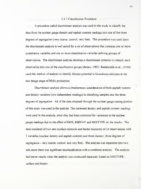
50
5.4.7 Classification Procedure
A procedure called discriminant analysis was used in this study to classify the
data from the nuclear gauge density and asphalt content readings into one of the three
degrees of segregation (very coarse, control, very fine). This procedure was used since
the discriminant analysis is well suited for a set of observations that contains one or more
quantitative variables and one or more classification variables defining groups of
observations. The discriminant analysis develops a discriminant criterion to classify- each
observation into one of the classification groups (James, 1985). Badaruddin et al., (1994)
used this method of analysis to identify distress potential in bituminous mixtures at the
mix design stage ofHMA production.
Discriminant analysis allows a simultaneous consideration of both asphalt content
and density variation (two independent readings) in classifying samples into the three
degrees of segregation. All of the data obtained through the nuclear gauge testing portion
of this study was used in the analysis. The corrected density and asphalt content readings
were used in this analysis, since they had been corrected for variations in the nuclear
gauge readings due to the effect ofDOS, BSEPAV and MIXTYPE on the results. The
data consisted of two sets (surface mixtures and binder mixtures) of 24 observations with
2 variables (nuclear density and asphalt content) and three classes ( three degrees of
segregation - very coarse, control, and very fine). The analysis was separated into two
sets since there was significant misclassification with a combined analysis. The analysis
had better results when the analysis was conducted separately based on MIXTYPE ,
surface and binder.

60
The discriminant analysis uses the method of Generalized Squared distance given
in equation 1. This equation can be used to classify any observation into one of the three
degrees of segregation distinguished in this study using the classification rule in equation
2.
D2(X,) = (X-X,)
TCOV- 1(X-Xj) ( 1
)
Where,
D 2(Xj) = Generalized Squared Distance from X to group j.
X = Sample Vector (Individual reading considered for classification)
Xj = Sample Mean Vector (Other readings already classified)
COV" 1 = Pooled Covariance Matrix
T = Transpose of a matrix
Observation X will be assigned to group j if,
D2(Xj) = min (D,
2, D 2
2, D,
2
) (2)
Results of the discriminant analysis are contained in Appendix D. Classification
and resubstitution information for each of the data sets is contained in Tables D.6 and
D.7 and Tables F. 13 and F. 14.
The analysis did not provide a zero error classification. Zero error classification
would be achieved if all of the data were classified correctly into their respective degrees
in Table D.7. One observation was misclassified for the binder mixtures as shown in
Table D. 14 The sample population from this study was invariably small and more data
may be needed to calibrate the model.
5.5 Permittivity
Permittivity was another candidate technology that was used to test the laboratory
prepared segregated mixtures. The hypothesis for use of this technology was based on
the assumption that every material has a unique set of electrical characteristics that are
dependent on its dielectric properties. The dielectric properties that were examined were
resistivity and permittivity. These properties are not constant and change with
temperature, orientation, pressure and molecular structure of the material being
measured. Resistivity is a DC-resistance measurement of a material High resistivity is
an important characteristic for insulating materials, while low resistivity is important for
conducting materials. A material is dielectric if it has the ability to store energy when
exposed to an external electric field.
5.5.1 Permittivity Theory
Permittivity, E, describes the interaction of a material with an electric field. The
dielectric constant, k*, is equivalent to relative permittivity, Er*= E*/En . Permittivity
consists of real and imaginary components. This relationship can be described as
follows:
Er* = k* = E*/E = (E'/E )-j(E"/E ) ( 1
)

62
where:
Er* = complex relative permittivity
E = permittivity in free space
Er
' = real part of permittivity
Er
" = imaginary part of permittivity.
The real part of permittivity is a measure ofhow much energy from an external electric
field is stored in a material and is always greater than one for most solids and liquids
The imaginary part of permittivity is also called the loss factor, and it is a measure of
dissipativeness of a material when exposed to an external electric field. It is always
greater than zero, but is usually much smaller than the real portion. The loss factor
includes the effects of both dielectric loss and conductivity.
A system for measuring permittivity includes a vector network analyzer, a coaxial
probe apparatus, an external computer and software. The system is based on the network
analyzer providing the high frequency stimulus and measures the reflected response. A
vector network analyzer consists of a signal source, a receiver and display. The source
sends a signal at a frequency to the material being tested. The receiver is tuned to the
transmitted frequency to detect the reflected and transmitted signals from the material.
The measured response produces the magnitude and phase data at the source transmitted
frequency. Subsequently, the input frequency is increased and the measurement
repeated. Software is then used to convert the measured data to permittivity, real and
imaginary. Relative permittivity values for some common materials are shown in Table
5.6.
5.5.2 Laboratory Measurement of Permittivity
Six gravel samples, three surface and three binder, were prepared using the
Purdue Linear Compactor. The samples for both types of mixtures included very coarse,
control (no segregation) and very fine mixtures. Permittivity of the six segregated
mixtures was measured using the test configuration shown in Figure 5.39. Measurements
were performed by Damaskos, Incorporated, Concordville, PA because of the uniqueness
of the test equipment.
Measurements were made using a Hewlett Packard 851 OB vector network
analyzer and Damaskos, Inc.'s propriety Inverted Arch. As indicated, the measurements
were made in a direct transmission mode over an input frequency range of 2 to 18 Ghz
using Damaskos' Arch Software. Using the transmission coefficients illustrated in
Figures 4.40 through 4.51, the dielectric constants of the six samples were computed as a
function of frequency. Figures 4.52 through 4.57 reveal that there is a clear difference in
the imaginary part of the dielectric constant for the three different levels of segregation
for each mix type. However, multiple samples of the same mixture at different levels of
segregation were not tested to statistically confirm this difference.
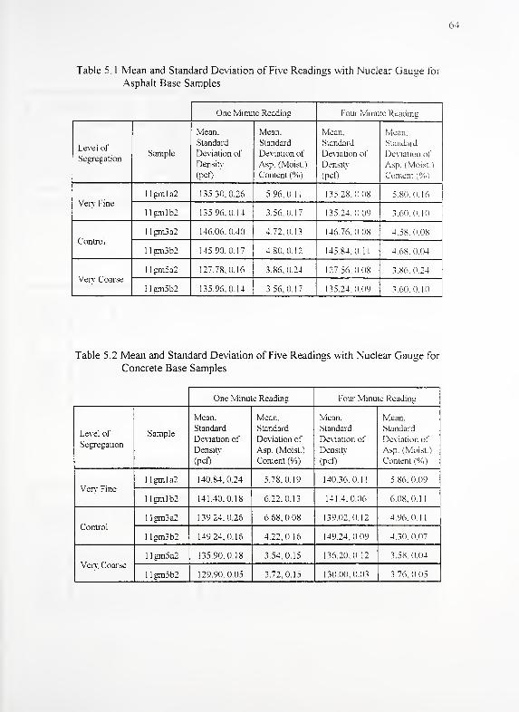
64
Table 5. 1 Mean and Standard Deviation of Five Readings with Nuclear Gauge for
Asphalt Base Samples
One Minute Reading Four Minute Reading
Level of
SegregationSample
Mean.
Standard
Deviation of
Density
(pcf)
Mean.
Standard
Deviation of
Asp. (Moist.)
Content (%)
Mean.
Standard
Deviation of
Density
(pcf)
Mean.
Standard
Deviation of
Asp. (Moist
)
Content (%)
Very Fine
1 1 gm 1 a2 135.30.0.26 5.96.0.11 135.28.0.08 5.80.0.16
llgmlb2 135.96,0.14 3.56.0.17 135.24.0.09 3 60. 0.10
Control
1 Igm3a2 146.06.0.40 4.72.0.13 146.76.0.08 4.58.0.08
Ilgm3b2 145.90, 0.17 4.80.0.12 145.84.0.11 4.68. 0.04
Very Coarse
I Igm5a2 127.78.0.16 3.86,0.24 127.56.0.08 3.86.0.24
1 1 gm5b2 135.96.0.14 3.56,0.17 135.24.0,09 3.60. 10
Table 5.2 Mean and Standard Deviation of Five Readings with Nuclear Gauge for
Concrete Base Samples
One Minute Reading Four Minute Reading
Level of
Segregation
Sample
Mean,
Standard
Deviation of
Density
(pcf)
Mean.
Standard
Deviation of
Asp. (Moist.)
Content (%)
Mean.
Standard
Deviation of
Density
(pcf)
Mean.
Standard
Deviation of
Asp. (Moist.)
Content (%)
Very Fine
1 1 gm 1 a2 140.84,0.24 5.78,0.19 140.36.0.11 5.86. 0.09
llgmlbZ 141.40,0.18 6.22,0.13 141.4.0.06 6.08.0.11
Control
1 Igm3a2 1 39.24. 0.26 6.68, 0.08 139.02.0.12 4.96. 0. 1 1
Ilgm3b2 149.24,0.16 4.22,0.16 149.24.0.09 4.30. 0.07
Very Coarse
1 Igm5a2 135.90.0.18 3.54.0.15 136.20.0.12 3.58. 0.04
I Igm5b2 129.90.0.05 3.72.0.15 130.00.0.03 3.76.0.05
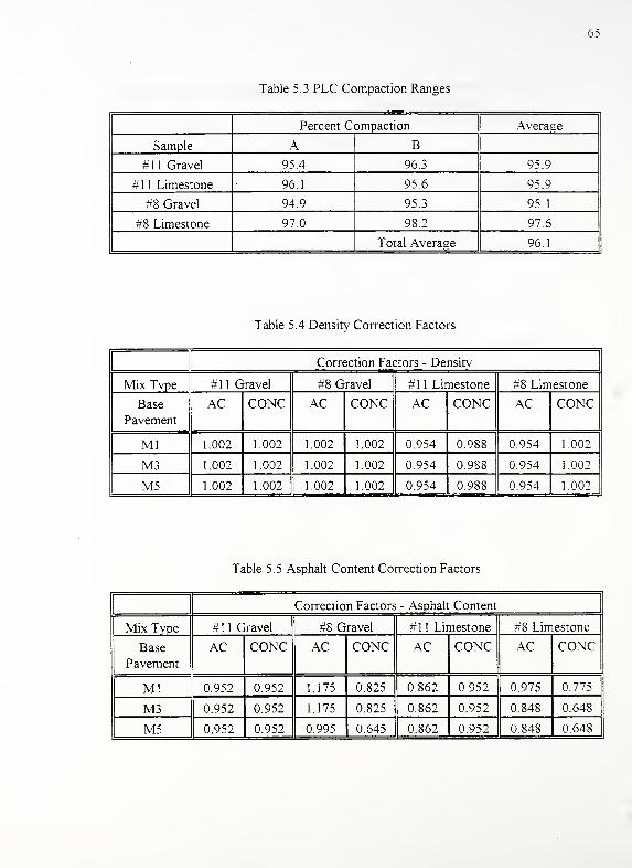
65
Table 5.3 PLC Compaction Ranges
Percent Compaction Average
Sample A B
#11 Gravel 95.4 963 95.9
#1 1 Limestone 96.1 956 95.9
#8 Gravel 94.9 95.3 95.1
#8 Limestone 97.0 98.2 97.6
Total Average 96 .1
Table 5.4 Density Correction Factors
Correction Factors - Densitv
Mix Type #11 Gravel #8 Gravel #1 1 Limestone #8 Limestone
Base
Pavement
AC CONC AC CONC AC CONC AC CONC
Ml 1.002 1.002 1.002 1.002 0.954 0.988 0.954 1.002
M3 1.002 1.002 1.002 1.002 0.954 0.988 0.954 1.002
M5 1.002 1.002 1.002 1.002 0.954 0.988 0.954 1.002
Table 5.5 Asphalt Content Correction Factors
Correction Factors - Asphalt Content
Mix Type #11 Gravel #8 Gravel #1 1 Limestone #8 Limestone
Base
Pavement
AC CONC AC CONC AC CONC AC CONC
Ml 0.952 0.952 1.175 0.825 0.862 0.952 0.975 0.775
M3 0.952 0.952 1.175 0.825 0.862 0.952 0.848 0.648
M5 0.952 0.952 0.995 0.645 0.862 0.952 0.848 0.648
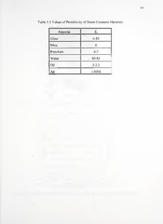
66
Table 5.6 Values of Permittivity of Some Common Materials
Material E r
Glass 6-10
Mica 6
Porcelain 6-7
Water .80-83
Oil 2-2.2
Air 1.0006
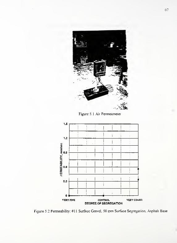
67
Figure 5.1 Air Permeameter
1.5
1.2
1S0.9
-i
sill 0.6s111
0.3
VERY FINE
I
|
! j|
!
!
!
i
:I i i 1 i
ii 11
CONTROL VERY COARSi
DEGREE OF SEGREGATION
Figure 5.2 Permeability: #1 1 Surface Gravel, 50 mm Surface Segregation. Asphalt Base
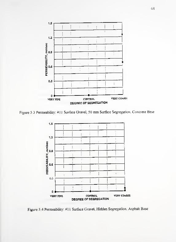
68
1.5
I
i i ! i i j
*
1.2
a|| ;
i
0)is
I ! !
:
I!
£ 0.9
> :
!
!
5<
1
«
uj 0.6 -
Sceuia
i
j j j
1 ( i j
0.3 -
! 1
1
i
VERY FINE CONTROL VERYCOA
DEGREE OF SEGREGATION
Figure 5.3 Permeability: #1 1 Surface Gravel, 50 mm Surface Segregation. Concrete Base
VERY FINE
T.b
i l i I I
I
'
\
| j
1.2
Ij I I I
i'
I I
!
0.9 -
! ! ! I !
j
I ! !I
I!
0.6 -
I j j I
|i : I i
j
1
!- i
CONTROL VERY COARSE
DEGREE OF SEGREGATION
Figure 5.4 Permeability: #1 1 Surface Gravel, Hidden Segregation, Asphalt Base
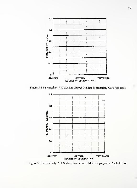
69
1.5
1.2
E0.9
03<ui 0.62Cu0.
0.3
VERY FINE CONTROL VERY COARSi
DEGREE OF SEGREGATION
Figure 5.5 Permeability: #1 1 Surface Gravel, Hidden Segregation, Concrete Base
1.5
1.2
E£0.9
m<w 0.6
cUJa.
. ! 1 1
VERY FINE CONTROL VERY COARSEDEGREE OF SEGREGATION
Figure 5.6 Permeability: #1 1 Surface Limestone, Hidden Segregation, Asphalt Base
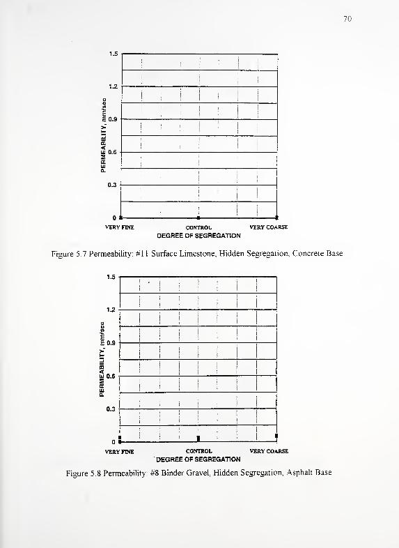
70
I.-3
1.2
o
iI
'
ii i
l ( I
CD
lo.9>
:
:
i
i!
;i
i
I
ffi
<til ft R
!i
2KUJ
I
a.
n *?
<{
I!
: |: |
0,: i
; i i
I
'
' i II
VERY FINE CONTROL VERY COARSE
DEGREE OF SEGREGATION
Figure 5.7 Permeability: #1 1 Surface Limestone, Hidden Segregation. Concrete Base
1.5
1.2
E£0.9
CD
uj 0.6EOCUJ0.
0.3
VERY FINE
i ! ! i I 1
'I
CONTROL VERY COARSE
DEGREE OF SEGREGATION
Figure 5.8 Permeability: #8 Binder Gravel, Hidden Segregation, Asphalt Base
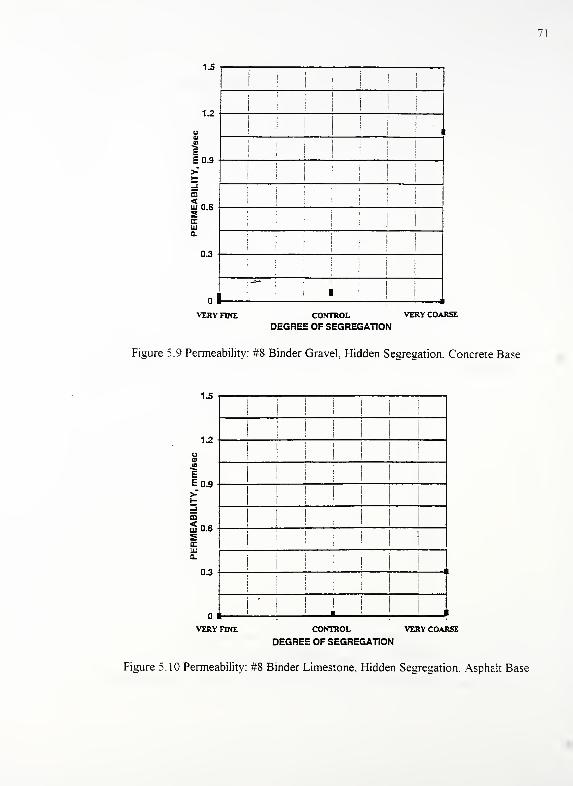
1.3
II |
i j I
1.2i i ! ! i
!!
I
! I i
0.9III III
i !
;
;
0.6
! | ! I iI
;• ' I
I
i
0.3 -
;i
i
i| I I
| |
i|
i
i
VERY FINE CONTROL VERY COARSE
DEGREE OF SEGREGATION
Figure 5.9 Permeability: #8 Binder Gravel, Hidden Segregation, Concrete Base
1.5
1.2
E£_0.9
>
mS 0.6
SECma
0.3
VERY FINE
|
I j i
"
I ! ! 1
CONTROL VERY COARSE
DEGREE OF SEGREGATION
Figure 5.10 Permeability: #8 Binder Limestone, Hidden Segregation, Asphalt Base
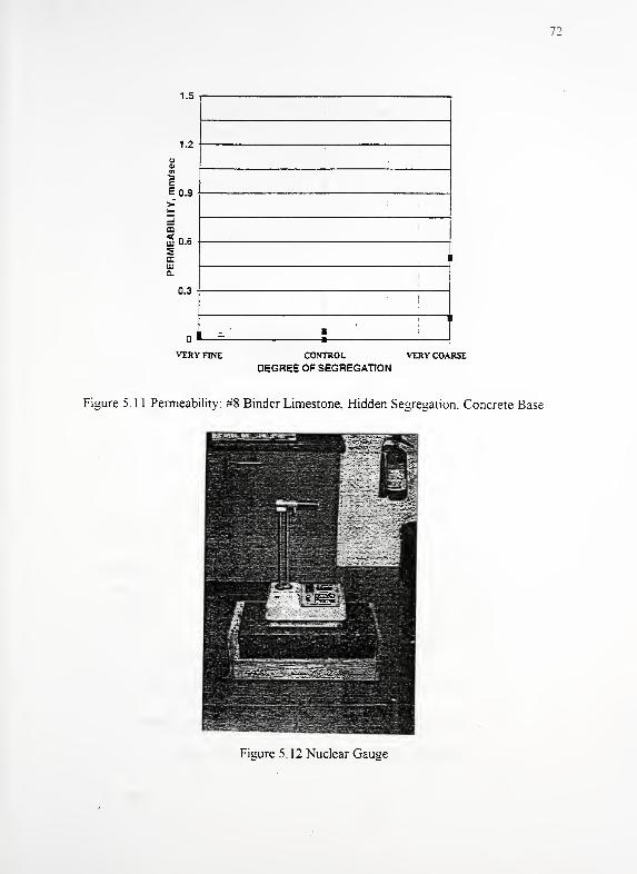
72
1.5
1.2
E£0.9
OD
2 0.6
5CUJa.
0.3
VERY FINE CONTROL VERY COARSE
DEGREE OF SEGREGATION
Figure 5.1 1 Permeability: #8 Binder Limestone, Hidden Segre»ation, Concrete Base
Figure 5.12 Nuclear Gauge
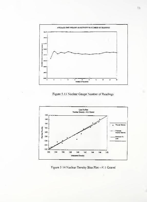
73
AVERAGE UNIT WIEGHT SENSITIVITY TO NUMBER OF READINGS
151 30
•2 IS100
t
M ISO so
i
2~ nci
£§< 14830
£
a 149.00
148.50
c 2 4 S 8 10 12 14 16 IS XNUMBER OP READINGS
Figure 5.13 Nuclear Gauge Number of Readings
148
Line Fit Plot
Nuclear Density - #1 1 Gravel
146 .
144 .
= 142 .
= 138 .
z
136 .
134 .
132 .
It?
^T 4>
^^^4>
Nuclear Density
^» • Predicted
Nuclear Density
Optimum Fit
Line
"8i: 2 134 136 138 140 142 144 146 U
Measured Density
Figure 5.14 Nuclear Density Bias Plot - #1 1 Gravel
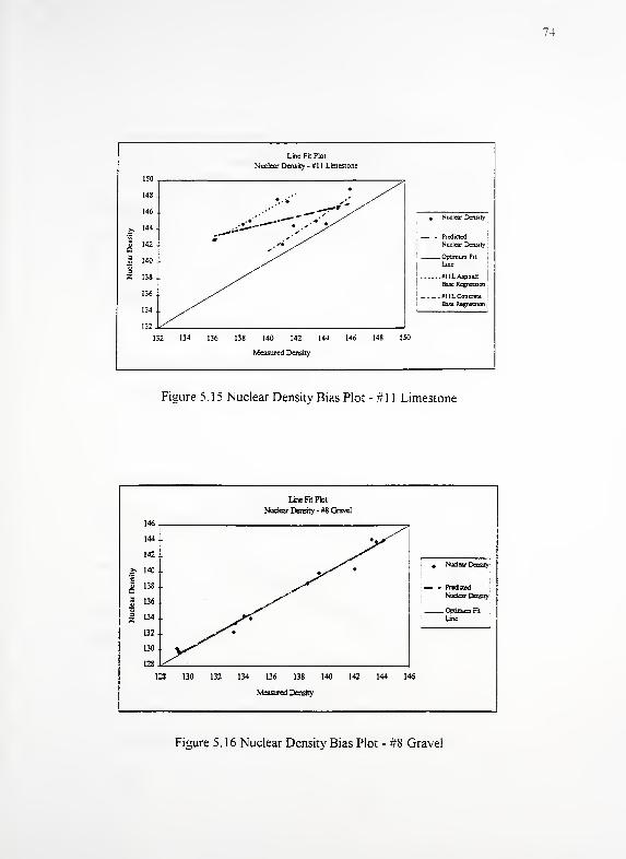
74
Z
150
Line Fit Plot
Nuclear Density - # 1 1 Limestone
148 .
146 .
144 .
142 .
140 .
138.
136.
134.
132
* Nuclear Density
— . Predicted
Nuclear Density
Optimum Fit
Line
| milLAsphalt !
Base Regression
jHI 1L Concrete
Base Regression
i: 2 134 136 138 140 142 144 146 148 1.
Measured Density
Figure 5.15 Nuclear Density Bias Plot - #1 1 Limestone
Line Fit Plot
Nuclear Density - #8 Gravel
* Nudear Density
' w m Predicted
Nudear Density
130 132 134 136 138 140
Measured Density
Figure 5. 16 Nuclear Density Bias Plot - #8 Gravel
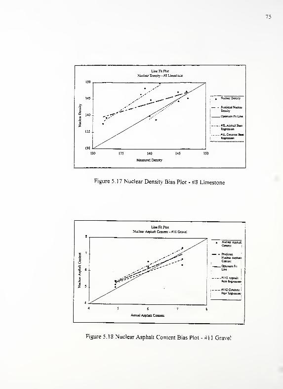
75
Line Fit Plot
Nuclear Density - #8 Limestone
140
Measured Density
» Nuclear Density
— • Predicted Nuclear
Density
Optimum Fit Lme
. DSL Asphalt Base
Regression
. «SL Concrete Base
Regression
Figure 5.17 Nuclear Density Bias Plot - #8 Limestone
Line Fit Plot
Nuclear Asphalt Content - * 1 1 Gravel
s
. Nuclear Asphalt
Content
.*S^- 7 . "\^^ — - Pfediaed
{: Nuclear AsphaltoU
1 6.±-£^"'' Content
Optimum Fit
Lme
<a **#^ ullGAsphalt
Base Regression* ^^
2 5 . *>r>^ i »I1G Concrete 1
4
4
Base Regression!
1 |
5 6 7 %
Actual Asphalt Content
Figure 5.18 Nuclear Asphalt Content Bias Plot - #1 1 Gravel
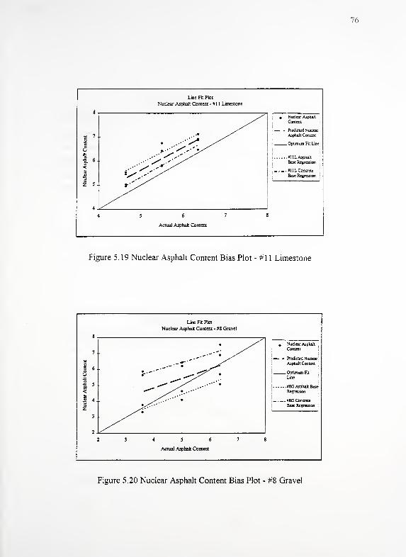
76
8 .
Line Fit Plot
Nuclear Asphalt Content -#11 Limestone
g? -
coU
I 6.
<
Z 5.
4
^ Nuclear Asphalt
Content
— - Predicted Nuclear
Asphalt Content
Opumum Fit Line
j
iUMlLAsphaJt
Base Regression
j
*11L Concrete
Base Regression
i 5 6 7 i
Actual Asphalt Content
\
Figure 5. 19 Nuclear Asphalt Content Bias Plot - #1 1 Limestone
Line Fit Plot
Nuclear Asphalt Content - #8 Gravel
^ - Predicted NudearAsphalt Content
Figure 5.20 Nuclear Asphalt Content Bias Plot - #8 Gravel
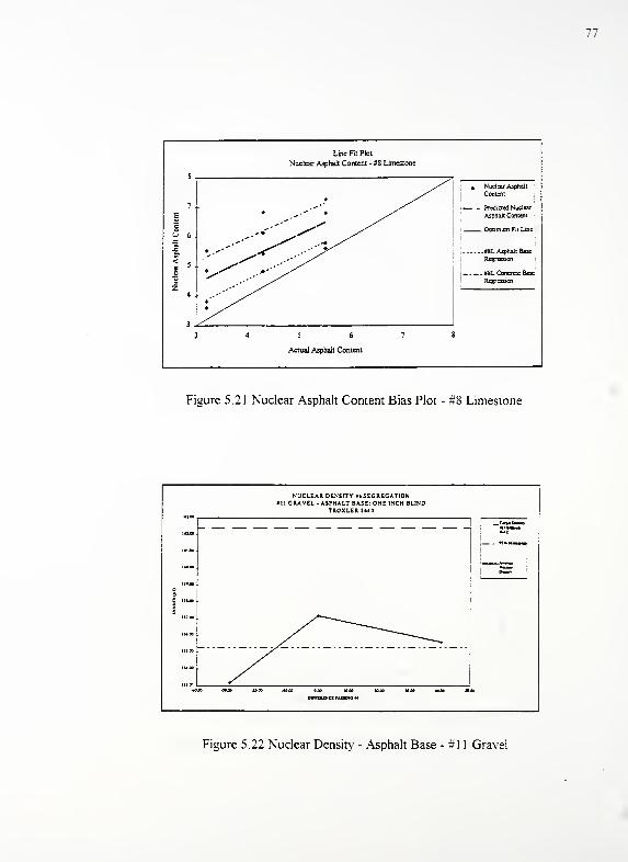
77
Line Fit Plot
Nuclear Asphalt Content - #8 Limestone
5 6
Actual Asphalt Content
— - Predicted Nuclear
Asphalt Contest
_ Optimum Fit Line
. =SL Asphalt Base
*8L Concrete £
Regression
Figure 5.21 Nuclear Asphalt Content Bias Plot - #8 Limestone
NUCLEAR DENSITY vi SEGREGATION111 GRAVEL -ASPHALT BASE: ONE INCH BLIND
TROXLER 3M0
1*1-00
110.00
Ie nigo
1
jn~ mmmm
^_^_/
m -Jtw oloo -iooo ooo iom um »j» mac mDIFTZUMCZ FASSOTO *4
Figure 5.22 Nuclear Density - Asphalt Base - #1 1 Gravel
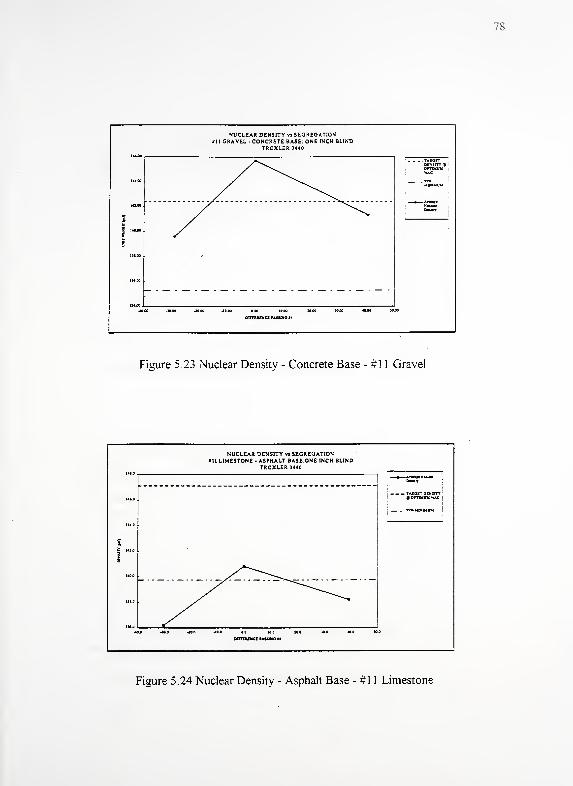
78
NUCLEAR DENSITY vi SEGREGATION*II GRAVEL - CONCRETE BASE: ONE INCH BLIND
TROXLER 3440
MM
I
1- - -
,DENSITY 4)
|
ofttmum|
." MINIMUM
•40130 -KM -1000 .10,00 000 10.00 1000 WOO MM KMormuxcE paisho »
Figure 5.23 Nuclear Density - Concrete Base - #1 1 Gravel
NUCLEAR DENSITY • SEGREGATION«l I LIMESTONE - ASPHALT BASE:0NE INCH BLIND
TROXLER 3440
, _ _ _ TAJtGET DENSITY9 0FTTMUMHAC
;
It K1J>a
3
/ ^^^-1C0 400 -100 10 100 100 M0 400 H
BOfUIHCXMSSIMH
Figure 5.24 Nuclear Density - Asphalt Base - #1 1 Limestone
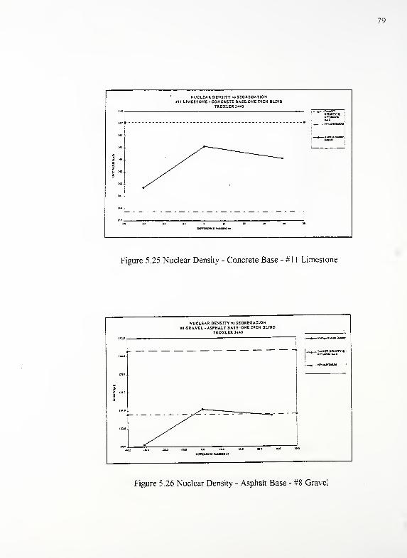
NUCLEAR DENSITY vi SEGREGATION«11 LIMESTONE - CONCRETE BASE:ONE INCH BLIND
TROXLER 3440
79
OfTMUUMAC
tMFFEUNCE rAUDIO »-
Figure 5.25 Nuclear Density - Concrete Base - #1 1 Limestone
NUCLEAR DENSITY »i SEGREGATION• I GRAVEL - ASPHALT BASE: ONE INCH BLIND
TROXLER 3440
offTUDicz passim} *
Figure 5.26 Nuclear Density - Asphalt Base - #8 Gravel
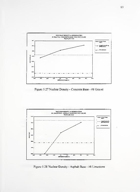
80
NUCLEAR DENSITY v> SEGREGATION«l GRAVEL - CONCRETE BASE: ONE INCH BLIND
TROXLER 3440
DITTTX£NCE FASJEWO 14
Figure 5.27 Nuclear Density - Concrete Base - #8 Gravel
NUCLEAR DENSITY »i SEGREGATIONII LIMESTONE - ASPHALT BASE ONE INCH BLIND
TROXLER 3440
MU
I
i
lJ4fl
IJ44
:
S.TAtCFTDCWSTTY
. .tlWMtNIMUH
/L> •HA JO* -lfl-0 «J> 10H 100 MO •#£ W
PmUKEMODIOM
Figure 5.28 Nuclear Density - Asphalt Base - #8 Limestone
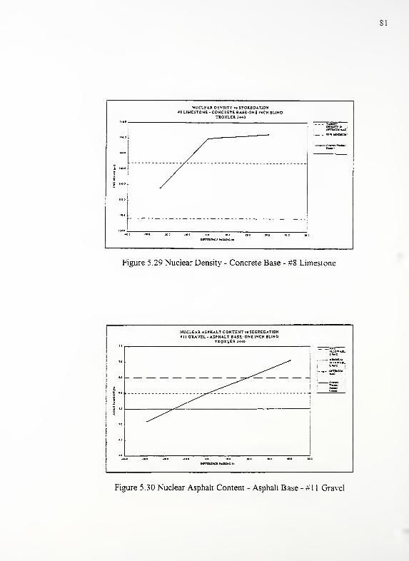
81
NUCLEAR DENSITY n SEGREGATION• t LIMESTONE - CONCRETE BASErONE INCH BLIND
TROXLER 3440
c
!*
111.0
/onM'Ju v.:
y.
tuntUNCE tAiSO*G **
Figure 5.29 Nuclear Density - Concrete Base - #8 Limestone
NUCLEAR ASPHALT CONTENT n SEGREGATION11 GRAVEL - ASPHALT BASE: ONE INCH BLIND
TROXLER 3440
i
!
i u5
-^^l-\_ _MA*
EveMWMWHALLOVAIL!v;
L «- .OfTOWXUK
^^^mttiidn:! paxsomo h
Figure 5.30 Nuclear Asphalt Content - Asphalt Base - #1 1 Gravel
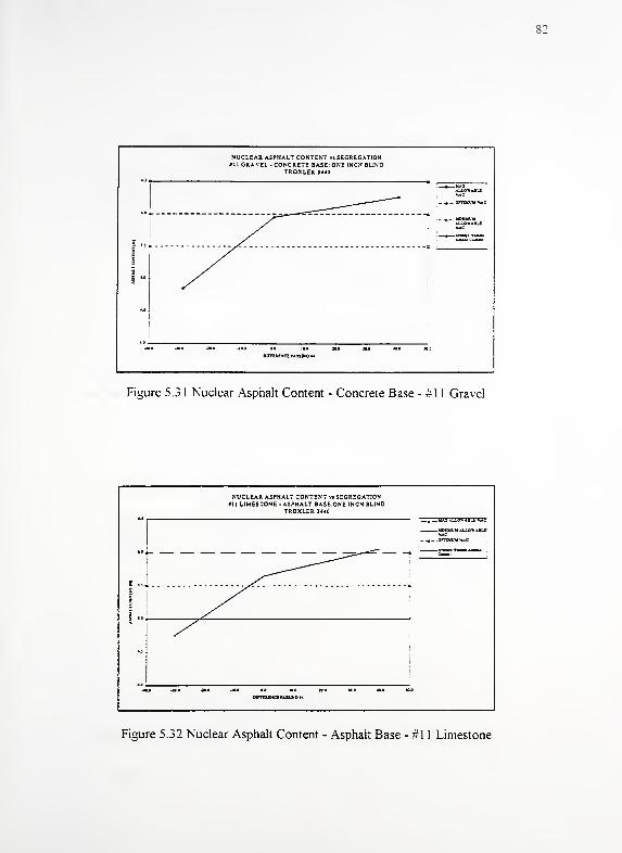
82
NUCLEAR ASPHALT CONTENT »| SEGREGATION• II GRAVEL - CONCRETE BASE: ONE INCH BLIND
TROXLER J440
DDTZUHCE PAJSOIO '
Figure 5.3 1 Nuclear Asphalt Content - Concrete Base - #1 1 Gravel
NUCLEAR ASPHALT CONTENT <n SEGREGATION• 11 LIMESTONE - ASPHALT BASE ONE INCH BLIND
TROXLER 3440
u,
-^—-^=r ^ —SS"—*—•
I u,
i
I
a
i
..
i
J> -K>0 -M4 iu oo io 20.0 m.o ma v>a
DffRBWCI fajiiwo «4
Figure 5.32 Nuclear Asphalt Content - Asphalt Base - #1 1 Limestone
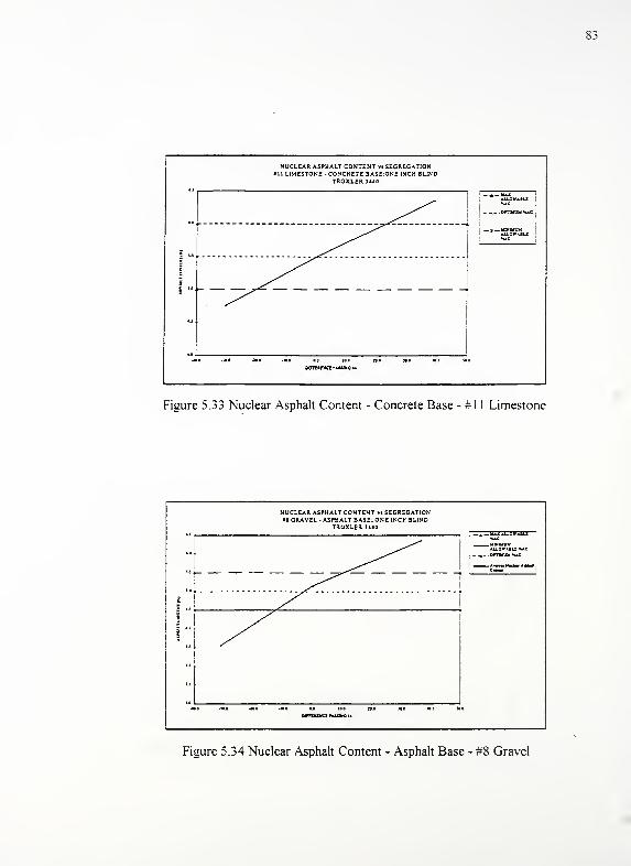
83
NUCLEAR ASPHALT CONTENT vi SEGREGATIONill LIMESTONE -CONCRETE BASE ONE INCH BLIND
TROXLER3*40
. „_ ,OPTIMUM XAC :
MO .10
wmMBtct rAumo *
Figure 5.33 Nuclear Asphalt Content - Concrete Base - #1 1 Limestone
NUCLEAR ASPHALT CONTENT »« SEGREGATION<8 GRAVEL - ASPHALT BASE: ONE INCH BLIND
TROXLER 3"0_ A B3 AU.OWABU
AU.OW4ILZ **C
Figure 5.34 Nuclear Asphalt Content - Asphalt Base - #8 Gravel
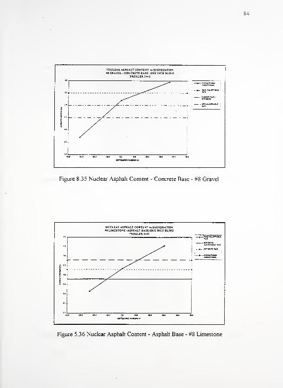
84
NUCLEAR ASPHALT CONTENT v» SEGREGATION*8 GRAVEL - CONCRETE BASE: ONE INCH BLIND
TROXLER 3«0
X Al_LO*AlU
H AU.OW A*L£
DVTUJXCt fAiSCiG «
Figure 8.35 Nuclear Asphalt Content - Concrete Base - #8 Gravel
NUCLEAR ASPHALT CONTENT vi SEGREGATION• 1 LIMESTONE -ASPHALT BASE ONE INCH BLIND
..
TROXLER 3**0A HAX UIOV4IU
HIMtMVMAU.OVAALE ^*C
^^" " *" ' **C
" ^^I" /^
c4*
5 u
/S
Li
pvfEUMci runa m
Figure 5.36 Nuclear Asphalt Content - Asphalt Base - #8 Limestone
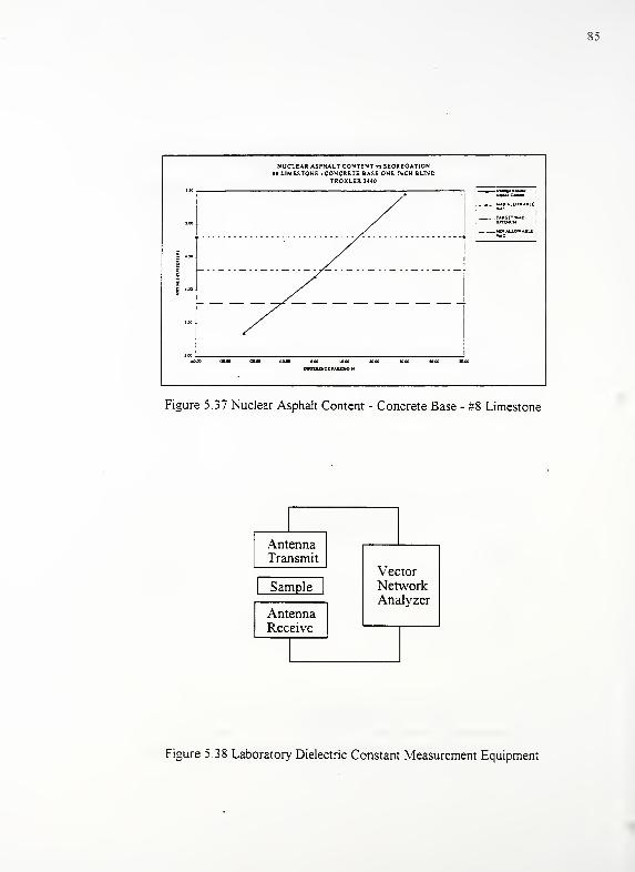
85
NUCLEAR ASPHALT CONTENT vi SEGREGATION«« LIMESTONE -CONCRETE BASErONE INCH BLIND
TROXLER 3440
DfFTOfHCE PAUDtO *•
Figure 5.37 Nuclear Asphalt Content - Concrete Base - #8 Limestone
AntennaTransmit
VectorNetworkAnalyzer
Sample
AntennaReceive
Figure 5.38 Laboratory Dielectric Constant Measurement Equipment
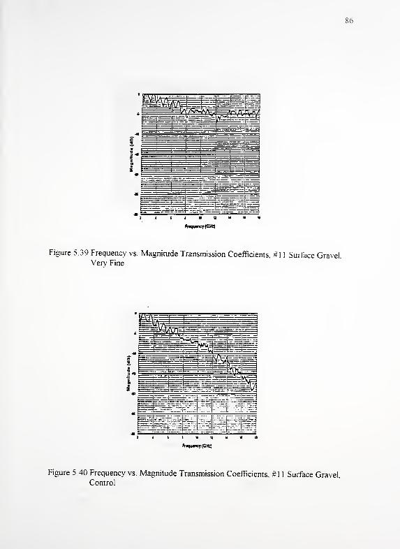
86
i-«.
' —01«3*
I
JO* '
'
" — ' ~i i iiasua*
Fraqut»qr(Ctt)
Figure 5.39 Frequency vs. Magnitude Transmission Coefficients, #1 1 Surface Gravel,Very Fine
-""-=- •" - •r;;t"r;=3
2 4 t i « s u « a
Froqwney (GHa
Figure 5.40 Frequency vs. Magnitude Transmission Coefficients, #1 1 Surface Gravel,
Control
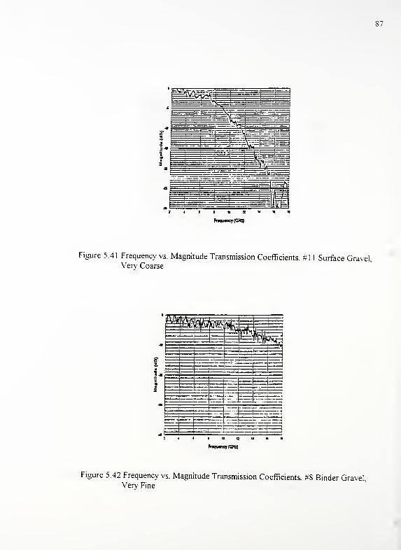
87
Figure 5.41 Frequency vs. Magnitude Transmission Coefficients, #1 1 Surface Gravel,Very Coarse
Figure 5.42 Frequency vs. Magnitude Transmission Coefficients, #8 Binder Gravel,Very Fine
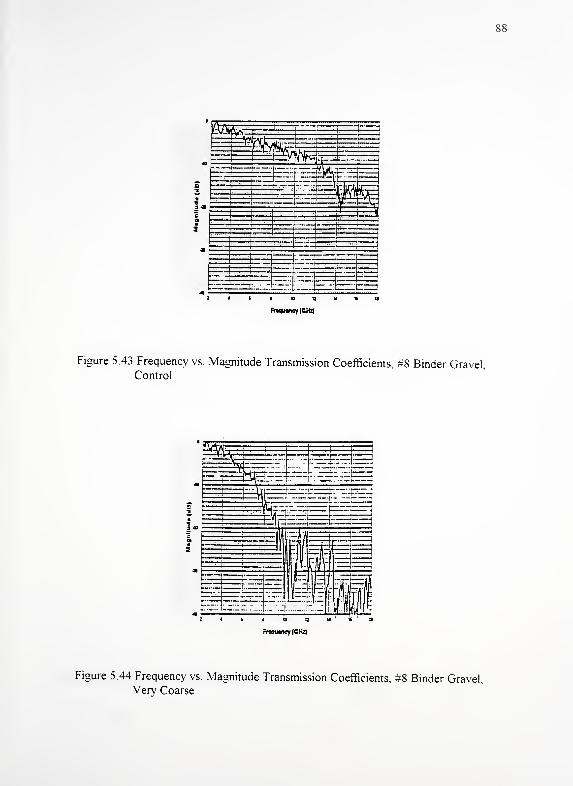
88
J 4 I i io a u % n
FraqiMncy(Ub)
Figure 5.43 Frequency vs. Magnitude Transmission Coefficients, #8 Binder Gravel,Control
Figure 5.44 Frequency vs. Magnitude Transmission Coefficients, #8 Binder Gravel,
Very Coarse
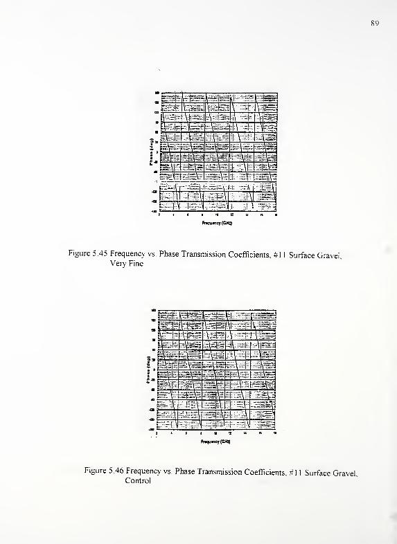
89
mmmmmi
:.M :MFrequtncy (CKS
Figure 5.45 Frequency vs. Phase Transmission Coefficients, #1 1 Surface Gravel,
Very Fine
Fraqutney (CH$
Figure 5.46 Frequency vs. Phase Transmission Coefficients, #1 1 Surface GravelControl
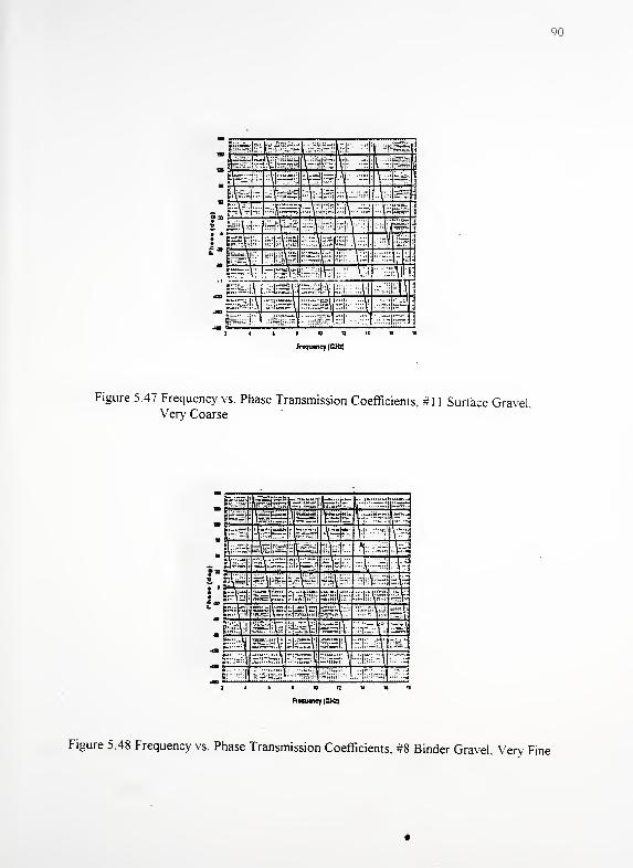
90
Frtqinnqr (CHz)
Figure 5.47 Frequency vs. Phase Transmission Coefficients, #1 1 Surface Gravel,Very Coarse
FuqiMnqr(CK4
Figure 5.48 Frequency vs. Phase Transmission Coefficients, #8 Binder Gravel, Verv Fine
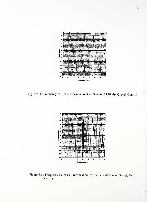
91
Fraqutncy (CKz)
Figure 5.49 Frequency vs. Phase Transmission Coefficients, #8 Binder Gravel, Control
Fraquauy (GHz)
Figure 5.50 Frequency vs. Phase Transmission Coefficients, #8 Binder Gravel, VeryCoarse
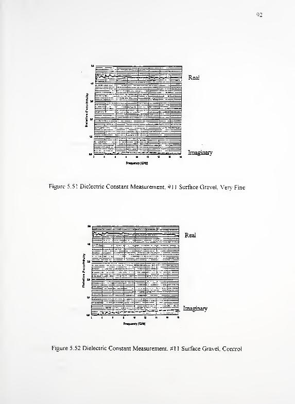
92
Real
—
—
;-/ "— I
—
M Imaginary
Figure 5.51 Dielectric Constant Measurement, #1 1 Surface Gravel, Very Fine
Figure 5.52 Dielectric Constant Measurement, #1 1 Surface Gravel, Control
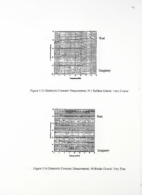
Imaginary
: < • i » a u » a
Friqumey (OJtt}
Figure 5.53 Dielectric Constant Measurement, #1 1 Surface Gravel, Very Coarse
Real
:^r^-igj====.-^—-^ Imaginarya u % %
Frequency (Cte)
Figure 5.54 Dielectric Constant Measurement, #8 Binder Gravel, Yen- Fine
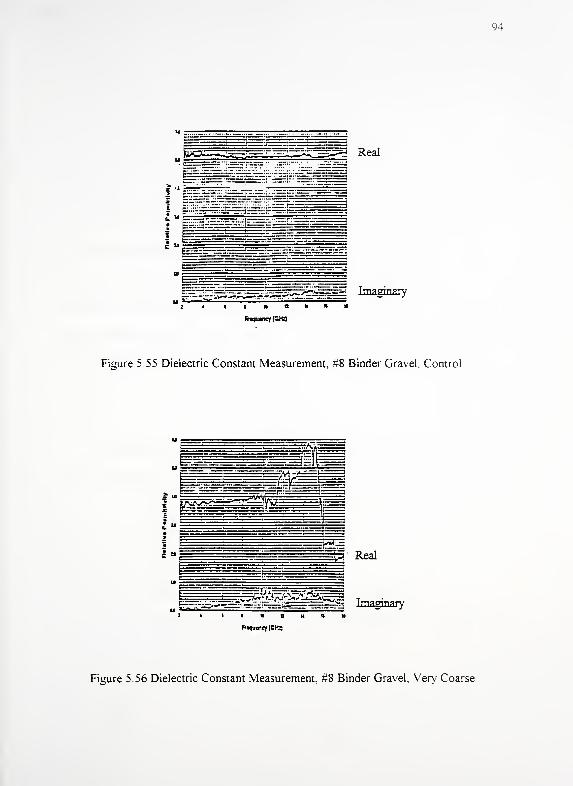
94
gpli5±=i^i=y5~j.^^;====s Imaginary
2 • I I
fnqumcf (CM)
Figure 5.55 Dielectric Constant Measurement, #8 Binder Gravel. Control
3 Real
j^5^-^v=^^^^!*^^s==^=^a ImaginaryI i a s u
faquenqr(CKQ
Figure 5.56 Dielectric Constant Measurement, #8 Binder Gravel, Very Coarse
95
CHAPTER 6. FIELD TESTS
6.1 Introduction
The previous laboratory study was conducted to determine which technologies
were viable for field implementation to detect segregation Based on these laboratory
tests and preliminary field testing, the nuclear gauge appeared to be the most promising
technology. Thus, an expanded field testing program was conducted using the nuclear
gauge to measure in-place moisture (asphalt) content and density Cores were taken at
the same location and analyzed in the laboratory.
6.2 Field Tests
Field projects tested were identified by the Indiana Department of Transportation
Operations personnel. These projects were as follows:
1. 1-469 North, 0.3 and 0.7 miles after the DuPont Road exit, right lane
with confinement from the left lane.
Fort Wayne, IN.
#8 Binder, limestone coarse aggregate and natural sand.
2. US 421 South, 1.4 and 0.8 miles from the Wabash River, right lane with
confinement from the right shoulder.
Delphi, IN.

96
#8 Binder, limestone coarse aggregate and natural sand.
3. 1-64 East on-ramp from SR 161, full-width paving lane without
confinement.
Holland, IN.
#9 Binder, limestone coarse aggregate and natural sand. The mix
design called for 17 percent recycled asphalt pavement
4. US 231 North, 0.6 miles north of Vincennes, right lane with
confinement from the left lane.
Vincennes, IN.
#8 Binder, limestone coarse aggregate and natural sand.
The Fort Wayne project was used as a trial section to evaluate the testing program. At
each project, two transverse sections were to be randomly located within two different
sublots. The first nuclear gauge readings for a transverse section were to be taken one
foot from the edge of paving lane. Subsequent readings were taken at one foot
increments across the lane until there was at least two feet but not less than one foot
remaining to the edge of the paving lane. In addition, by visual inspection, sites within
the sublot were located and tested that appeared to be segregated, coarse and fine, and
non-segregated. The Holland project was limited, consisting of only one sublot. It also
started to rain at the Holland project before tests of the visually located sites were
completed.
97
6.2. 1 Preliminary Field Tests
As noted, the Fort Wayne project was used as a trial project. A problem was
encountered when field nuclear density was compared with the saturated surface dry
density of cores. This problem is depicted in Figures 6.1 and 6.2. The paraffin coating
technique was not utilized because the asphalt was to be extracted.
On the Fort Wayne project, the nuclear gauge readings were taken the following
day after paving. There was significant scatter in comparing the moisture (asphalt)
content readings and extracted asphalt contents of the cores shown in Figures 6.3 and 6.4.
It was surmised and confirmed through conversations with the nuclear gauge
manufacturer (Brown, K., 1995), that the readings should be taken the same day.
immediately after compaction Otherwise, moisture from rain or humidity penetrating
the mat's surface would affect the gauge readings. As a result, on the ensuing three
projects the readings and cores were taken the same day as construction
6.2.2 Expanded Field Tests
Field tests were conducted on the three remaining projects. At these projects,
nuclear gauge readings were taken just after compaction of the pavement mat to
minimize any errors in the moisture (asphalt) content readings due to humidity Density
readings were also recorded concurrently with the asphalt content readings The field
nuclear readings are summarized in Tables 6.1 through 6.3 for the additional projects.
The transverse readings for density and moisture (asphalt) content are shown in Figures
6.5 through 6.9 and Figures 6.10 through 6.14, respectively.

98
6 3 Laboratory Analysis
To examine whether a relationship between the nuclear gauge readings and the
actual pavement existed, 20.3 cm cores were taken in the exact locations where the
nuclear gauge measurements were recorded These cores were taken by the Indiana
Department of Transportation Research Division and Vincennes District personnel.
The laboratory analysis was initially envisioned to involve measuring the
saturated surface dry density of the cores, performing an extraction to determine the
asphalt content, and performing a sieve analysis. However, results from the Fort Wayne
project (Figure 6.2) indicated either the nuclear gauge or the core saturated surface dry
densities were in error. As a result, on the remaining three projects a volumetric density
measurement technique was employed in addition to the saturated surface dry method.
6.3.1 Density
Core density was initially measured by the saturated surface dry technique given
in ASTM D-2726. Core density was also determined utilizing a technique outlined by
White ( 1 975) which assumes the cores are right cylinders. The height and diameter of a
subject core is measured at three equidistant locations. The average height and the
diameter of the cylinder are then used to calculate the volume of the cylinder.
Subsequently, the dry weight ofthe core is divided by the calculated volume to determine
the density.
99
6.3. 1 .
1
Bulk Density Evaluation
Based on the relation of saturated surface dry (SSD) bulk density and nuclear
density on the Fort Wayne project, it was hypothesized that the constant density reflected
in the SSD density was a result of water that had penetrated the cores' connected air
voids when the submerged weight was obtained Subsequently, the water drained during
preparation prior to obtaining the saturated surface dry weight This would result in a
lower volume and thus a higher density. The following equation outlines the calculation
of bulk specific gravity (ASTM D-2726).
Bulk Specific Gravity = [A/(B-C)] ( 1
)
where:
A = mass in grams of sample in air,
B = mass in grams of saturated surface-dry specimen in air,
C = mass in grams of sample in water.
It is obvious that a decrease in the value of B results in a lower bulk density. The bulk
densities for the transverse sections are shown in Figures 6.5 through 6.9. The values for
the three subsequent test locations are shown in Tables 6.1 through 6.3.
6.3.1.2 Volumetric Density
Volumetric density was calculated assuming the cores were right cylinders
Height and diameter of the cores were measured at three equidistant locations The
100
average height, diameter and the dry weight were then used to calculate the cylindrical
volumetric (CV) density. The CV densities for the transverse sections are shown in
Figures 6.5 through 6.9. Values for the three subsequent test locations are shown in
Tables 6.1 through 6.3.
6.3.1.3 Comparison of Different Densities: Random Locations
To determine the relationship between SSD and CV densities and four minute
nuclear density readings, regression analysis was performed on data obtained from
random locations transverse to pavement laydown. The following equation was used in
the analysis to compare the densities.
SSD, CV = A(Nuc) + B (2)
where:
SSD = Saturated Surface-Dried Density,
CV = Cylindrical Volumetric Density,
Nuc = Four Minute Nuclear Gauge Density Reading,
A, B = Regression Coefficients.
This analysis was performed separately on data obtained from random sublots Two
random sublots were sampled on the Delphi and Vincennes projects, and one sublot on
the Holland project
6.3.1.3.1 Delphi Project
The regression results performed on data from the two Delphi sublots are
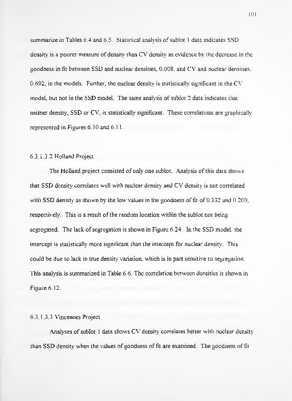
101
summarize in Tables 6.4 and 6.5. Statistical analysis of sublot 1 data indicates SSD
density is a poorer measure of density than CV density as evidence by the decrease in the
goodness in fit between SSD and nuclear densities, 0.008, and CV and nuclear densities.
0.692, in the models. Further, the nuclear density is statistically significant in the CV
model, but not in the SSD model. The same analysis of sublot 2 data indicates that
neither density, SSD or CV, is statistically significant. These correlations are graphically
represented in Figures 6. 10 and 6. 1
1
6.3.1.3.2 Holland Project
The Holland project consisted of only one sublot. Analysis of this data shows
that SSD density correlates well with nuclear density and CV density is not correlated
with SSD density as shown by the low values in the goodness of fit of 0.332 and 0.209,
respectively. This is a result of the random location within the sublot not being
segregated. The lack of segregation is shown in Figure 6.24. In the SSD model, the
intercept is statistically more significant than the intercept for nuclear density. This
could be due to lack in true density variation, which is in part sensitive to segregation
This analysis is summarized in Table 6.6. The correlation between densities is shown in
Figure 6.12.
6.3.1.3.3 Vincennes Project
Analyses of sublot 1 data shows CV density correlates better with nuclear density
than SSD density when the values of goodness of fit are examined. The goodness of fit
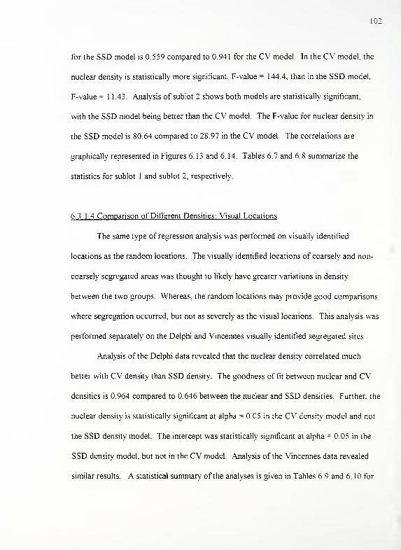
102
for the SSD model is 0.559 compared to 0.941 for the CV model. In the CV model, the
nuclear density is statistically more significant, F-value = 144.4, than in the SSD model.
F-value = 1 1.43. Analysis of sublot 2 shows both models are statistically significant,
with the SSD model being better than the CV model. The F-value for nuclear density in
the SSD model is 80.64 compared to 28.97 in the CV model. The correlations are
graphically represented in Figures 6.13 and 6.14. Tables 6.7 and 6.8 summarize the
statistics for sublot 1 and sublot 2, respectively.
6.3. 1 .4 Comparison of Different Densities: Visual Locations
The same type of regression analysis was performed on visually identified
locations as the random locations. The visually identified locations of coarsely and non-
coarsely segregated areas was thought to likely have greater variations in density
between the two groups. Whereas, the random locations may provide good comparisons
where segregation occurred, but not as severely as the visual locations This analysis was
performed separately on the Delphi and Vincennes visually identified segregated sites
Analysis of the Delphi data revealed that the nuclear density correlated much
better with CV density than SSD density. The goodness of fit between nuclear and CV
densities is 0.964 compared to 0.646 between the nuclear and SSD densities. Further, the
nuclear density is statistically significant at alpha = 0.05 in the CV density model and not
the SSD density model. The intercept was statistically significant at alpha = 0.05 in the
SSD density model, but not in the CV model. Analysis of the Vincennes data revealed
similar results. A statistical summary of the analyses is given in Tables 6.9 and 6. 1 for
io;
the Delphi and Vincennes sites, respectively. The relationship between the three
densities are shown in Figures 6. 1 5 and 6. 16 for the Delphi and Vincennes sites,
respectively.
6.3.2 Asphalt Content
Asphalt content of the field samples was determined by extraction of the asphalt
according to ASTM D-2172, Method B. The results are shown graphically in Figures
6. 1 7 through 6.21 Regression analysis was done for each subot comparing four minute
nuclear gauge moisture (asphalt) content and extracted asphalt content The goodness of
fit for all sublots ranged from 0.11 to 0.45 showing that a strong relationship does not
exist. However, when the same regression was performed for the visually located
segregated locations, the goodness of fit for the Delphi and Vincennes projects are 0.59
and 0.95. This shows that visually identified locations have larger variations in asphalt
content from the job mix formula and that the nuclear gauge can be used to detect these
variations. The values for the three expanded test locations are shown in Tables 6.
1
through 6.3.
6.3.3 Gradation
Core aggregate gradation after asphalt extraction was determined according to
ASTM D-448. Based upon the job mix formulas for each project, the sieve that most
nearly divided the gradation evenly was identified. This sieve was the 9.5 mm sieve for
the Delphi and Vincennes projects (INDOT 25 mm nominal maximum mixture) and the
104
4.75 mm sieve for the Holland project (INDOT 19 mm nominal maximum mixture). The
percent passing this sieve was subtracted from the actual percent passing of each core for
the appropriate project. Results of the transverse locations are shown graphically in
Figures 6.22 through 6.26. The values for the three expanded test locations are shown in
Tables 6. ] through 6.3. Sieve analysis for the Fort Wayne project samples was not
performed because of the incomplete CV density data and inappropriate field testing with
the nuclear gauge as discussed previously.
6.4 Classification
The same procedure, discriminant analysis, used in Chapter five to classify the
segregated laboratory samples using nuclear gauge readings was used to classify field
samples. However, base pavement and mixtype variables previously included in the
laboratory classification were not used in the field classification. Further, only two
categories, coarse and non-coarse segregation, were used in the field classification For
this analysis, a sample was categorized as being "coarse segregation" if the gradation was
more than five percent above the job mix formula on the 9.5 mm sieve, otherwise the
sample was categorized as "no coarse segregation." Discriminant analysis, was used to
analyze samples from the visually identified segregated and non-segregated sites. The
independent variables are the nuclear gauge moisture (asphalt) content and density
readings.
Initially, all of the data (transverse sections and visual sites) were classified using
the nuclear density and moisture (asphalt) content. This classification was conducted
105
using the SAS discriminant analysis procedure (SAS Institute, 1988). Classification
using all of the data created a bias towards the "none" segregated set because of there
being more "none" data. Using the data for visually located segregated, coarse and fine,
and non-segregated locations resulted in poor classification. This is caused by the
physical properties of fine segregation Visually identifying what appears to be fine
segregation created problems because the "fine" segregation may be only a very thin
layer on the surface. Whereas with the coarse segregation, the coarser aggregate does
constitute a thicker layer of the segregation.
Subsequently, the data for visually identified sites was classified alone with a 100
percent success in the classification. These results are summarized in Table 6.11.
Analysis was based on a plus or minus five percent passing on the 9.5 mm sieve for the
Delphi and Vincennes projects. The 9.5 mm sieve was selected because for both job mix
formulas, this sieve evenly divided the mix as 50/50 retained/passing. As previously
mentioned, the visual data set for Holland was incomplete due to rain The results of the
discriminant analysis are in Appendix E. Figure 6.27 was prepared from the discriminant
analysis of the visual data. The lines of posterior probability shown in Figure 6.26 apply
to coarsely identified locations only.
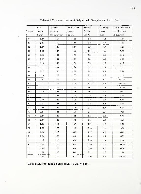
106
Table 6. 1 Characterization of Delphi Field Samples and Field Tests
Sample
Bulk
Specific
Gravity
Cylindrical
Volumetric
Specific Gravity
Extracted .Asp.
Content.
percent
Nuclear*
Specific
Gravity
Nuclear .Asp.
Contem.
percent
Dill', in Grad. on 9.5
nun Sieve Irani
JMF. percent
l.A 2.27 2.03 4.65 2. IX 4.2 -3.64
IB 2.26 2.09 4.54 2.18 4.7 -1.69
1C 2.27 2.16 5.14 2.28 4.X -5.23
ID 2.24 2.23 4.X0 2.51 4.6 7.33
IE 2.2X 2.22 4X6 2.36 5.3 0.14
IK 2.27 2.21 4.63 2.34 5.2 5. 81
1G 2.25 2. IX 5.14 2.28 5.6 6.17
1H 2.21 2.21 5.34 2.32 5.4 11.15
11 2.27 2.20 4.79 2.42 4.9 1.7X
1.1 2.26 2.09 5.50 2.25 4.7 -7.03
IK 2.31 2.09 4.97 2 27 4.1 -:: -5
1L 2.22 2.0X 4.0X 2.22 43 -14.78
KA 2.27 2.06 4.27 2.05 4.9 -10.03
XB 2.26 2.13 5. IX 2.00 4.9 -0.17
XC 2.2X 2.15 5.29 2.10 5.3 1 .00
XD 2.24 2.16 6.05 2.16 5.5 9.34
8E 2.26 2.13 4.98 2.16 5.4 1.04
8F 2.24 2.14 5.08 2.27 5.4 X.73
XG 2.26 2.11 4.94 2.31 5.1 -0.91
XH 2.25 217 4.85 2.33 5.2 9.7X
XI 2.27 2.11 4.7X 2.35 5.3 -2.57
XI 2.26 2.06 4.83 2.29 4.9 1.79
XK 2.29 2.05 4.41 2.26 4.8 -3.2X
XL 2.2X 2.17 4.83 2.17 4.X -4.XX
2 2.2X 2.19 4.40 2.00 5.1 -6.71
3 2.27 2.02 5.28 2.20 5.4 0.24
4 2.26 2.22 6.21 2.16 5.5 14.56
5 2.29 2.00 4.14 1.99 4.7 -9.74
6 2.2X 2.07 4.6X 2.21 5.5 1X4
7 2.30 2.03 4.21 1.96 4X -16.99
* Converted from English units (pef) to unit weight.
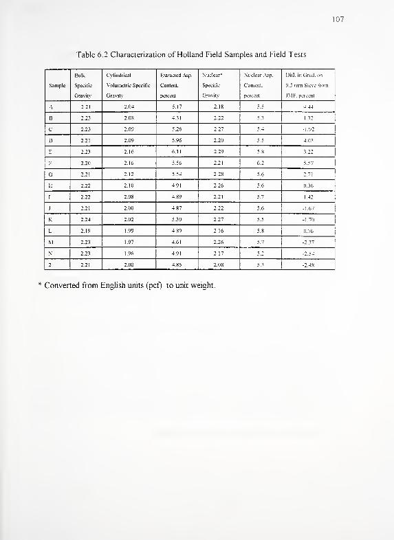
107
Table 6.2 Characterization of Holland Field Samples and Field Tests
Sample
Bulk
Specific
Gravity
Cylindrical
Volumetric Specific
Gravity
Extracted .Asp.
Content.
percent
Nuclear*
Specific
Gravity
Nuclear Asp.
Content,
percent
Dill inCiracJ
9 5 nini Sieve
.IMF. percent
from
A 2.21 2.04 5.17 2.18 5.5 4 44
B 2.23 2.08 4.31 2.22 5.3 1 32
C 2.23 2.09 5.26 2.27 5.4 -1.92
D 2.21 2.09 5.96 2.20 5.5 4 03
E 2.23 2.16 6.11 2.29 5.8 } ::
r 2.20 2.16 5.56 2.21 6.2 5.57
Ci 2.21 2.12 5.54 2.28 5.6 2.71
H 2.22 2.10 4.91 2.26 5.6 36
I 2.22 2.08 4.89 2.21 5.7 1 42
.1 2.21 2.00 4.87 2.22 5.6 -1.67
K 2.24 2.02 5.30 2.27 5.5 -1.70
L 2.19 1.99 4.89 2.16 5.8 0.76
M 2.23 1.97 4.61 2.26 5.7 -2.37
N 2.23 1.96 4.91 2.17 5.2 -2.54
2 2.21 2.00 4.85 2.08 5.3 -2.48
Converted from English units (pef) to unit weight.
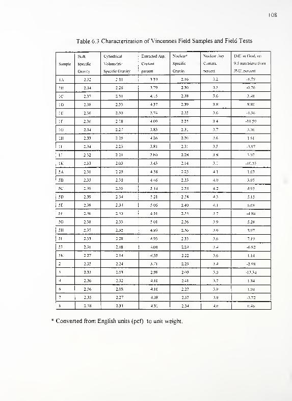
108
Table 6.3 Characterization of Vincennes Field Samples and Field Tests
Sample
Bulk
Specific
Gravity
Cylindrical
Volumetric
Specific Gravity
Extracted Asp.
Content.
percent
Nuclear*
Specific
Gravity
Nuclear .Asp
Content.
percent
Dill, in Grad. on
9.5 nun Sieve from
JM1'. percent
1A 2.32 2.11 3.39 2.16 3.2 -X.79
IB 2.34 2.26 3.79 2.30 3.5 -0.76
1C 2.37 2.31 4.15 2.38 3.6 3.48
ID 2.38 2.33 4.37 2.39 3.8 8X0
IE 2.36 2.30 3.74 2.35 3.6 -1.36
IP 2.36 2.18 4.09 2.25 3.4 -10.59
1G 2.34 2.27 3.83 2.31 3.7 3.06
1H 2.33 2.25 4.26 2.30 3.6 1.61
11 2.34 2.23 3.81 2.31 3.5 -3.97
U 2.32 2.21 3.80 2.28 3.8 3.07
IK 2.33 2.03 3.43 2.14 3.1 -10.35
5.A 2.31 2.29 4.38 2.23 4.1 1.03
5B 2.35 2.30 4.46 2.33 4.0 3.97
5C 2.39 2.35 5 14 2.38 4.2 4.91
5D 2.39 2.34 5.21 2.38 4.3 5.15
5E 2.38 2.34 5.06 2.40 4.1 6.08
5F 2.36 2.30 4.51 2.33 3.7 -4 84
5G 2.38 2.3.3 5.01 2.36 3.9 5.28
5H 2.37 2.32 4.93 2.36 3.9 3.97
51 2.33 2.28 4.93 2.33 3.6 7.19
5.1 2.31 2.18 4.08 2.24 3.4 -6.82
5K 2.27 2.14 4.39 2.22 3.6 1.14
: 2.35 2.24 3.71 2.23 3,4 -2.98
3 2.33 2.03 2.98 2.09 3.0 -13.34
4 2.36 2.32 4.10 2.41 3.7 1.34
6 2.36 2.18 4.10 2.27 3.9 1.94
7 2.35 2.27 438 2.37 3.9 -3.72
X 2.38 2.31 4.31 2.34 4 0.46
* Converted from English units (pcf) to unit weight.
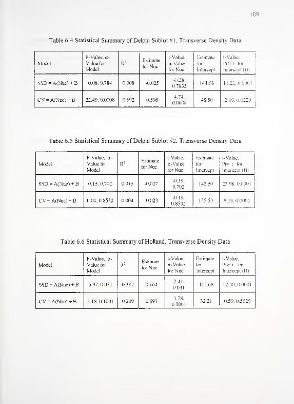
109
Table 6.4 Statistical Summary of Delphi Sublot #1, Transverse Density Data
Model
F-Value. De-
Value for
Model
R :Estimate
for Nuc
t- Value.
a-Value
for Nuc
Estimate
for
Intercept
l- Value.
I'r> t for
Intercept (B)
SSD = A(Nuc) + B 0.08,0.784 0.008 -0.025-0.28.
0.7835144 68 1 1.21, 0.0001
GV = A(Nuc) + B 22.49. 0.0008 0.692 0.5964.74.
0.000848.50 2.69. 0.0229
Table 6.5 Statistical Summary of Delphi Sublot #2. Transverse Density Data
Model
F- Value, a-
Value for
Model
R :Estimate
for Nuc
t-Value.
a- Value
for Nuc
Estimate
for
Intercept
t-Value.
Pr> i for
Intercept (B)
SSD = A(Nuc) + B 0.15.0.702 0.015 -0.017-0.39.
0.702143.50 23. 9S. 0.0001
CV = A(Nuc)+B 0.04. 0.8532 0.004 -0.023-0.19,
0.85321 35.53 8.19. 0.0001
Table 6.6 Statistical Summary of Holland, Transverse Density Data
Model
F- Value, a-
Value for
Model
R :Estimate
for Nuc
t-Value.
a- Value
for Nuc
Estimate
for
Intercept
t-Value.
Pr> l for
Intercept (B)
SSD = A(Nuc) + B 5.97.0.031 0.332 0.1642.44,
0.031115.68 12.40.0.0001
CV = A(Nuc) + B 3.18,0.1001 0.209 0.6931.78.
0.100132.21 59. 0.5629
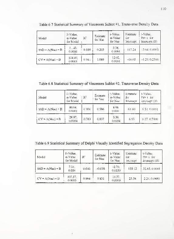
10
Table 6.7 Statistical Summary of Vincennes Sublot #1, Transverse Density Data
Model
F-Value.
a-Value
for Model
R :Estimate
for Nuc
t-Value.
a-Value
for Nuc
Estimate
for
Intercept
I- Value.
Pr> t tor
Intercept (13)
SSD = A(Nuc)+B11.43.
0.00810.559 0.203
3.38.
0.0081117.24 1 3 64. O.OOO'l
CV = A(Nue) + B144.40.
0.00010.941 1 .089
12.02.
0.0001-16.65 -1.29.0.2306
Table 6.8 Statistical Summary of Vincennes Sublot #2, Transverse Density Data
Model
F-Value.
a-Value
for Model
R :Estimate
for Nuc
t-Value.
a-Value
for Nuc
Estimate
for
Intercept
t-Value,
Pr> t for
Intercept (B)
SSD = A(Nuc) + B80.64.
0.00010.900 0.586
898.
0.00016 1 .60 6.51. 0.0001
CV= A(Nuc) + B28.97.
0.00040.763 0.937
5.38.
0.00046.93 0.27. 0.7900
Table 6.9 Statistical Summary of Delphi Visually Identified Segregation Density Data
Model
F-Value.
a-Value
for Model
R :Estimate
for Nuc
I- Value.
a-Value
for Nuc
Estimate
for
Intercept
l-Value.
Pr> t for
Intercept (13)
SSD = A(Nuc) + B7.31,
0.0540.646 -0.098
-2.70.
0.0539155.12 32.85.0.0001
CV = A(Nuc) + B107.57.
0.00050.964 0.831
10.37.
0.000523.38 2.24. 0.0889
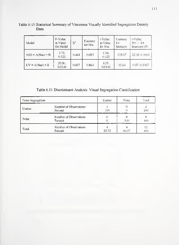
Table 6.10 Statistical Summary of Vincennes Visually Identified Segregation Density
Data
Model
F-Value.
a- Value
for Model
R : Estimate
tor Nuc
t-Value.
a- Value
for Nuc
Estimate
for
Intercept
l-Valuc.
1T> t for
Intercept (Bi
SSD = A(Nuc) + B3.75.
0.1250.484 0.083
1.94.
0.125135.07 22.05.0.0001
CV = A(Nuc) + B20.50.
0.01060.837 0.864
4.53.
0.010615.64 0.57. 0.5967
Table 6. 1 1 Discriminant Analysis: Visual Segregation Classification
From Segregation Coarse None Total
Number of ObservationsCoarse „
Percent
4
100
4
100
Number of ObservationsNone „
Percent
8
100
X
100
_ , Number of Obsei"vationsTotal nPercent
4
3 3 . 3 3 66.67
12
100
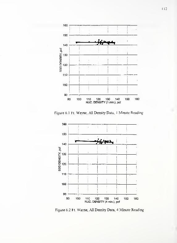
112
160
150
140
cozLU
Q 120oCOCO
110
100
90
; j
'
: | ! |
_
i j ; j|
j |j j i I |
ii i l i
!|
!i
!
|!
90 100 110 120 130 140 150 160
NUC. DENSITY (1 min.), pcf
Figure 6.1 Ft. Wayne, All Density Data, 1 Minute Reading
160
150
140
130
120
110
100
90 -
i ; I I
! i -—-ViWu.- s =
i ; II
j
; i : :i-ii!
I
: ! I
I;
II I
!i
i I;
!
:
! ! !
90 100 110 120 130 140 150 160NUC. DENSITY (4 min.), pcf
Figure 6.2 Ft. Wayne, All Density Data, 4 Minute Reading
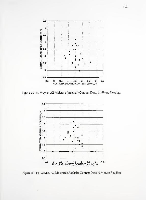
6.5 -
6 -
5.5
5 -
4.5
3.5
1
:
!
j
1
I1
2.5
1 .'. *
1
'! 1
i
i i
ii
! ! | i
: ! ! !
2.5 3 3.5 4 4.5 5 5.5 6 6.5
NUC. ASP. (MOIST.) CONTENT (1min.), %
Figure 6.3 Ft. Wayne, All Moisture (Asphalt) Content Data, l Minute Reading
6.5
^ 6
I-"
a: 5.5l-z8 5
!:<14.50.W<Q 4inI-O<3.5-
2.5
|| !
:
! ill!! -
;
i i
i
i
I
! 1 1 i
!
1
! '
l
! i
1 I
i
I
- i 1 1
\ 1
i
:
I
!
|1 ! !
i
1 | 1"
i
! ill! |
2.5 3 3.5 4 4.5 5 5.5 6 6.5
NUC. ASP. (MOIST.) CONTENT (4 min.), %
Figure 6.4 Ft. Wayne, All Moisture (Asphalt) Content Data, 4 Minute Reading
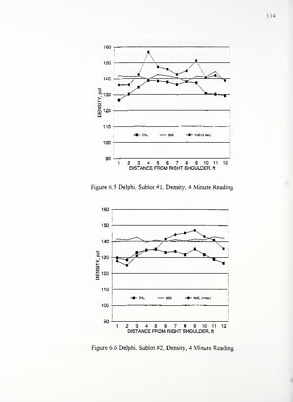
14
110 -
100
901 2 3 4 5 6 7 8 9 10 11 12
DISTANCE FROM RIGHT SHOULDER, ft
Figure 6.5 Delphi, Sublot #1, Density, 4 Minute Reading
160
150
140
•130
120
110
100
90
|!
i ;
_^ _ ^r^>^~-^* V
\^V *-.
-9- CYL SSO -•- NUC. (4 mil.)
1 2 3 4 5 6 7 8 9 10 11 12
DISTANCE FROM RIGHT SHOULDER, ft
Figure 6.6 Delphi, Sublot #2, Density, 4 Minute Reading
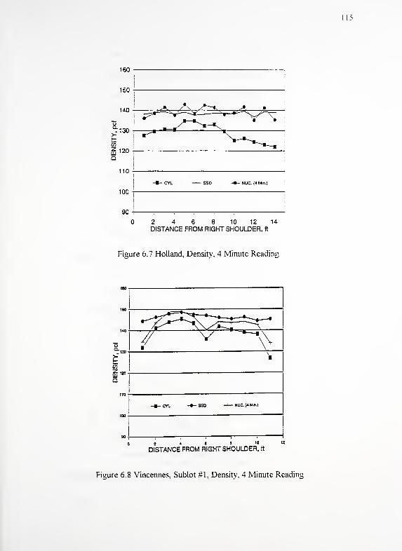
2 4 6 8 10 12 14
DISTANCE FROM RIGHT SHOULDER, ft
Figure 6.7 Holland, Density, 4 Minute Reading
180
^^^Ei^i
1
v -^>1-
.
Q
-*- en. -- SSO —r— NUC. (4 Min.)
90
DISTANCE FROM RIGHT SHOULDER, ft
Figure 6.8 Vincennes, Sublot #1, Density, 4 Minute Reading
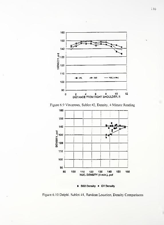
2 4 6 8 10 12
DISTANCE FROM RIGHT SHOULDER, ft
Figure 6.9 Vincennes, Sublot #2, Density, 4 Minute Reading
160
150
140
JT130
120
1
110
100
90
I
i
! !
|
!i
!
!i
,*s*
i
i
• ]
i
I
90 100 110 120 130 140 150 160
NUC. DENSITY (4 min.), pcf
SSD Density • CV Density
Figure 6.10 Delphi, Sublot #1, Random Location, Density Comparisons
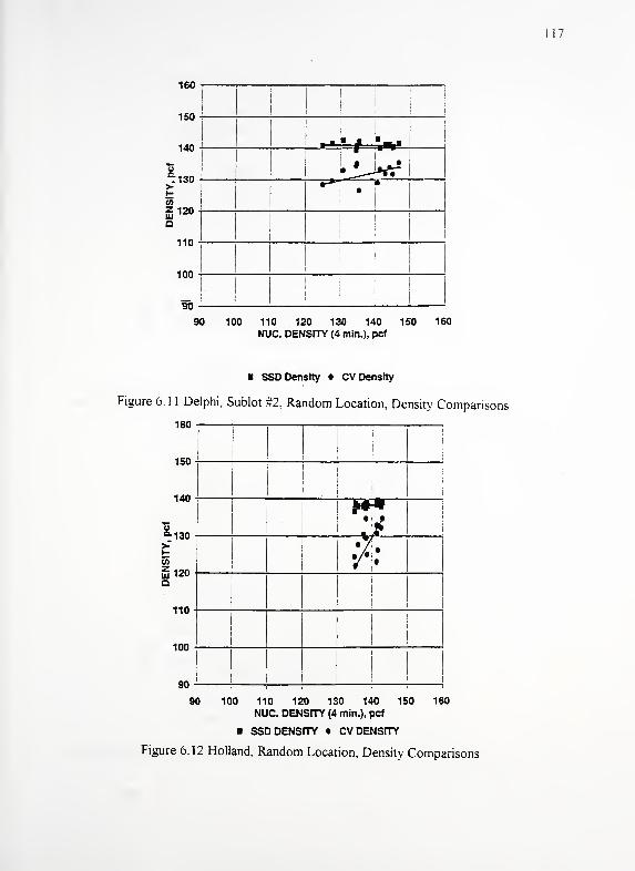
117
160
150
140
130
120
110
100
90
90 100 110 120 130 140 150 160
NUC. DENSITY (4 min.), pcf
SSD Density • CV Density
Figure 6. 11 Delphi, Sublot #2, Random Location, Density Comparisons
160
150
140
0-130>55
g 120
110
100
90
i
i
i
i
! i
! ***I
I
\
i
! I !
I—
i
90 100 110 120 130 140 150 160
NUC. DENSITY (4 min.), pcf
SSD DENSITY • CV DENSITY
Figure 6. 12 Holland, Random Location, Density Comparisons
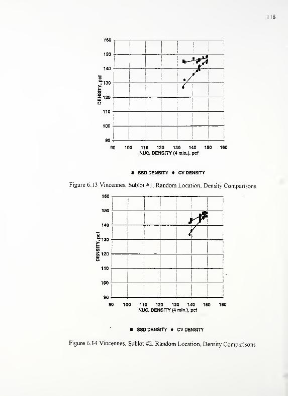
160
150
140
:130
enz 120
a
110
100
90
J
90 100 110 120 130 140 150 160
NUC. DENSITY (4 min.), pcf
SSD DENSITY * CV DENSITY
Figure 6 13 Vincennes, Sublot #1, Random Location, Density Comparisons
160i
|
I
! i
140 '
!! HZ
o
>55Z 19D
Q
inn -
90 -
90 100 110 120 130 140 150 160
NUC. DENSITY (4 min.), pcf
SSD DENSITY • CV DENSITY
Figure 6. 14 Vincennes, Sublot #2, Random Location, Density Comparisons
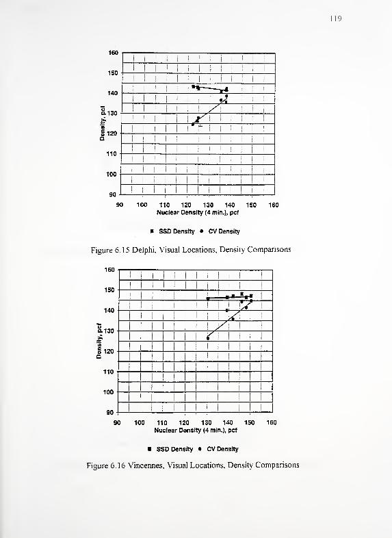
19
1i i
i
;
!
i
'
1
! i i i Ii i ; !
i ii
1 1 1 1 1i i'i 1 ! ! i 1
** T§1 1 1 ! 1 i 1 1 U! ! 1 .1
|J/l
!! 1 jf
ii i i i r i
i
i ! 1 1: ! i
;
! | !i
1 1 1 1 ! ! 1 ! ! ii i 1
II
! ! 1 1 1 1
III ! i 1 ii 1 1
1 1 1 1 I 1
1
i Mil II
160
150
140
"oa 130
Ȥ120a
110
100
90
90 100 110 120 130 140 150 160
Nuclear Density (4 min.), pcf
SSD Density • CV Density
Figure 6. 1 5 Delphi, Visual Locations, Density Comparisons
160
150
140
aO.130
a5120Q
110
100
90
90 100 110 120 130 140 150 160
Nuclear Density (4 min.), pcf
SSD Density • CV Density
Figure 6.16 Vincennes, Visual Locations, Density Comparisons
11
1 II II1 1 1 1 i
1i i i
1 1 1 ! 1 1
'i
1 1 1 1 1 1 1 1 1 ,! IVf !
1 1i
1 i 1 1 i ! Vl 1 !
1 ! I 1 KM 1 1
( i
1 i
i
!
1 1 1 ! i 1
i II i 1
1 II 1 1 II II1 1 1 |
1 1i
1 il 1i 1
I
III 1
1
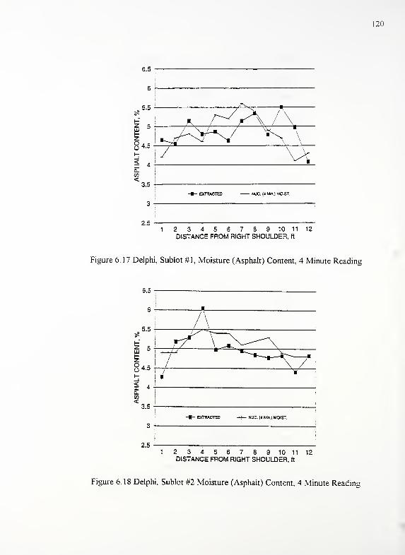
120
6.5
6
5.5
2 5
K
84.51-
O.
<3.5
3
2.5
"^ I
R KAA! ^<f*V ^S \
1/i
v>1
-- EXTRACTED NUC. (4 Mm.) MOIST.
i
1 2 3 4 5 6 7 8 9 10 11 12
DISTANCE FROM RIGHT SHOULDER, ft
Figure 6.17 Delphi, Sublot #1, Moisture (Asphalt) Content, 4 Minute Readinu
1 2 3 4 5 6 7 8 9 10 11 12DISTANCE FROM RIGHT SHOULDER, ft
Figure 6.18 Delphi, Sublot #2 Moisture (Asphalt) Content, 4 Minute Reading
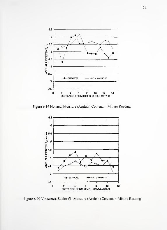
121
NUC. (4 Min.) MOIST.
3 -
2.5
2 4 6 8 10 12 14DISTANCE FROM RIGHT SHOULDER, ft
Figure 6.19 Holland, Moisture (Asphalt) Content, 4 Minute Readim
6.5
15.5
Z111
^4.5OOS 4<X0-
52 3.5
2.5
-
rA . Ax^v X>7\i^ V
\-•- BCTRACTED —
i
— NUC. (4 Min.) MOIST.
i
;
1
2 4 6 8 10
DISTANCE FROM RIGHT SHOULDER, ft
12
Figure 6.20 Vincennes, Sublot #1, Moisture (Asphalt) Content, 4 Minute Reading
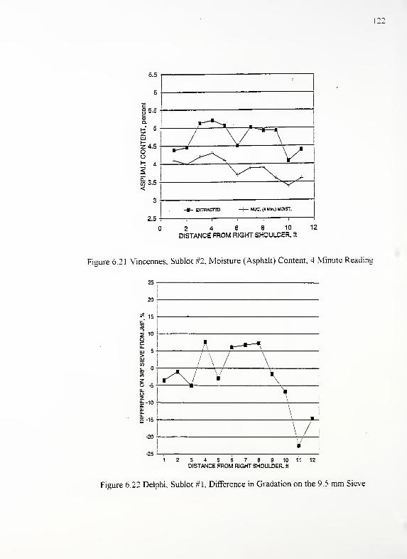
122
2 4 6 8 10 12
DISTANCE FROM RIGHT SHOULDER, ft
Figure 6.21 Vincennes, Sublot #2, Moisture (Asphalt) Content, 4 Minute Reading
25 -
20 -
u.
22 10 foau.
uj 5 4-
> j
1zo .-^ T7 \o|-10UJu.u.5-15
-20/
-25
1 2 3 4 5 6 7 8 9 10 11 12
DISTANCE FROM RIGHT SHOULDER, ft
Figure 6.22 Delphi, Sublot #1, Difference in Gradation on the 9.5 mm Sieve
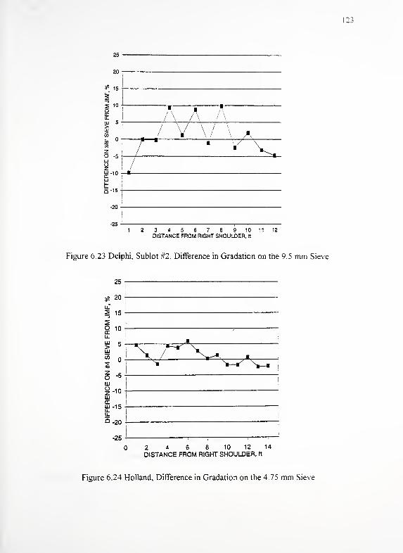
25
20
15
ITu. A /\ ' \
>
? o!
/ V \/ \ ACO °53
Z° -5
l
X " v v^% 17LU
5-15
-20
-25
1 2 3 4 5 6 7 8 9 10 11 12
DISTANCE FROM RIGHT SHOULDER, ft
Figure 6.23 Delphi, Sublot #2, Difference in Gradation on the 9.5 mm Sieve
25
20
15
10
5
-5
10
•15
a -20
-25
X̂i"
2 4 6 8 10 12 14
DISTANCE FROM RIGHT SHOULDER, ft
Figure 6.24 Holland, Difference in Gradation on the 4.75 mm Sieve
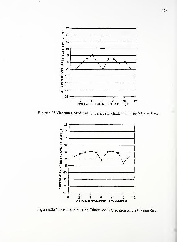
124
2 4 6 8 10 12
DISTANCE FROM RIGHT SHOULDER, ft
Figure 6.25 Vincennes, Sublot #1, Difference in Gradation on the 9.5 mm Sieve
- 20
3«o£ 10in
uj 5 •
CO
2 o-UJX
I- - Tl t *-
**-* \/I -^ —
v1
oo•z.m -15tc 1SUJu.u- -?n -
Q-25
2 4 6 8 10 12
DISTANCE FROM RIGHT SHOULDER, ft
Figure 6.26 Vincennes, Sublot #2, Difference in Gradation on the 9.5 mm Sieve
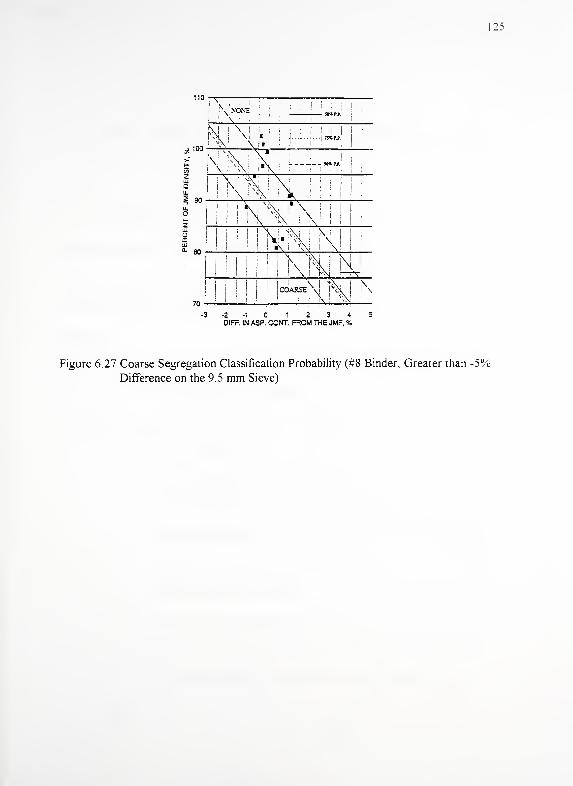
125
100
90
: Yi \ ;
NONE I
I! ! )
'!
|
: ! .\'
1 i
M I \ Mm n r.
|
• :
!
! i
| ;
J }..-| 73%P.P 1
K^\
j\. J 90* PJ.'
I
i \ i
!! i\aiH'IIMII
I I I i
1
1 1 K %j !\! ! 1 1
'
801
1
1 IK'XJ NJ'
1
1
1
1
1
i \\W\l
1
1 \;
^n
1 1 i 1 I 1 !coarse\! 1M N-3-2-10 1 2 3 4
DIFr. IN ASP. CONT. FROM THE JMF, %
Figure 6.27 Coarse Segregation Classification Probability (#8 Binder, Greater than -5%
Difference on the 9.5 mm Sieve)
126
CHAPTER 7. FLEXURAL FATIGUE TESTING OF SEGREGATED MIXTURES
7 1 Introduction
Flexural fatigue testing was performed to examine the difference in fatigue of
procurement and preparation of samples, test apparatus, testing procedures, results and
analysis.
7.2 Preparation of Samples for Fatigue Testing
Samples were prepared in a multi-step process. This process included:
1
.
Drying aggregate to a constant weight,
2. Sieving aggregate into stockpiles by size,
3
.
Recombining aggregate to satisfy required gradation,
4. Heating combined aggregate and asphalt to predetermined mixing
temperature based on the asphalt viscosity,
5. Mixing aggregate and asphalt,
6. Curing mix for approximately one hour,
7. Preheating Purdue Linear Compactor (PLC) mold to compaction
temperature using an infrared heater shown in Figure 7.1,

127
8 Compacting slabs in the PLC (slab dimensions of 102 mm high by 550
mm long and 305 mm wide) to their predetermined laboratory density
as discussed in Chapter 4,
9 Saw three beams measuring approximately 380 mm long by 75 mm
wide by 75 mm high using a water-cooled diamond saw blade (Figure
7.2). Figures 7.3 and 7.4 show the beams' layout on a schematic of
the slabs,
10. Drying beams to a constant weight at room temperature
Once the beams reached a constant weight, the final weight and
dimensions were determined and recorded. These measurements
allow the density and cross-sectional area of each specimen to be
calculated. The cross-sectional area is used in the strain calculation
for the flexural fatigue test.
1 1
.
Bonding an indented aluminum button to the center of each beam with
epoxy. The probe of the linear variable differential transducer
(LVDT) is placed in the indenture of the button to minimize
movement. The LVDT measures beam vertical displacement
12. Placement of beams in an environmental chamber for 3 hours to
allow the specimens to reach 25 degrees Celsius prior to testing.
There was some difficulty in producing quality beams for the binder, very coarse level of
segregation. The saw blade raveled the poorly bonded coarse aggregate from the
mixture.
128
7 3 Test Apparatus
A Materials Testing Systems Corporation (MTS) electro-hydraulic testing
machine was used for applying loads to the beam specimens. The beams were held in a
load frame built for repeated flexural tests and was contained within an environmental
chamber capable of maintaining a constant temperature within 0.5 degrees Celsius.
A Shaevitz type GCD- 120-050 linear variable differential transducer (LVDT) was
used to measure the deflection of a subject beam during testing. The tip of the LVDT
was placed in the indenture of the aluminum button that was previously bonded to the
center of the test beam. The MTS system and repeated flexure frame in the
environmental chamber are shown in Figures 7.5 and 7.6, respectively LABTECH
NOTEBOOK software (Labtech Notebook, 1991) was used to record data automatically
using a 12 bit DT2801-A A/D conversion board mounted in a personal computer. The
strain level was manually controlled by monitoring the voltage level of the LVDT using
an oscilloscope.
7.4 Test Procedures
Prior to installation of a beam in the flexural test apparatus, the loading clamps
were adjusted vertically to the same level as the support/reaction clamps. The centers of
the two support/load clamps are 50 mm from the beam center and 100 mm from the
centers of two reaction clamps. Two layers of teflon were placed between a subject beam
and the clamps to reduce friction which could cause shearing stresses near the clamps
creating moment in the test portion of a specimen.
129
All beams were tested in a controlled strain mode at 25 degrees Celsius using a
one hertz haversine wave with a 0. 1 second loading period and a 9 second rest period.
A specimen is tested at a predetermined constant deflection. This deflection is used to
calculate the extreme fiber strain using the following equation
Strain, in/in = (12H*D)/(3L2-4A2
) (1
)
where:
H = Specimen height, inches
D = Deflection of the beam at the center, inches
L = Reaction span length, inches
A = Distance between support and first applied load, inches
As a specimen fatigues, it requires a lower load to attain the desired deflection (i.e. this
stiffness decreases). Beams were tested until the flexural stiffness modulus was 50
percent of the initial stiffness modulus measured at the 200th load application Data
acquisition was performed automatically by a personal computer with the Labtech
Notebook software interacting with an MTS control board.
7.5 Fatigue Test Results
The fatigue results for the surface gravel mixture are shown in and Tables 7.
1
through 7.5. Results for the gravel binder mixture are shown in Tables 7.6 through 7.10.
All of the results for the two mix sizes and different levels of segregation exhibit the
typical trend associated with decreasing strain: an increase in the number of cycles to
failure (Yoder and Witzak, 1975).

7.6 Analysis
Two types of statistical analysis of the fatigue test results were performed In the
first, a regression analysis of data for each level of segregation was conducted separately
Predictive equations for each level of segregation for both gravel mixes were
developed. The predictive equations were of the form shown in Equation 1 because the
analysis was performed on translated data. The data was translated by taking the
logarithm to the base 10 of both the strain and number of cycles to failure.
Log 10(Nf)= A + BxLog 10(e) (2)
where:
N, = Number of cycles to failure,
e = Strain, in/in, and
A, B = Regression Constants.
This equation is then presented in its classical form in equation 3 (Yoder and Witzak,
1975).
Nr
=k(l/e)c (3)
where:
k, C = values based on regression constants.
However, the analysis presented here is based on the following equation.
Nr
= D(e)B
(4)
131
where:
D = 10\
A, B = Regression constants defined in equation 2
The F-values for the models and regression variables are shown in Table 7.11. The
values of B and D for the models, as expressed in equation 2, are listed in Table 7.12.
The predicted fatigue equations for the gravel surface and binder mixtures with the five
levels of segregation are shown in Figures 7.7 and 7.8, respectively.
In the second analysis, a regression was performed by mix size with all five levels
of segregation. The logarithm of strain to the base 10, level of segregation and the
interaction between the two variables were included in the model. Level of segregation
was used as a class variable. The purpose of this analysis was to examine the levels of
segregation and test whether the performance of the different levels of segregation was
statistically different. The form of this model for both the surface and binder mixtures
was as follows.
Log 10(Nf) = A + BxLog]0(e) + DxLOS + ExLog
10(s)* LOS (5)
where:
LOS = Level of Segregation (1, 2, 3, 4, 5),
D, E = Regression Constants.
Table 7. 1 3 summarizes the model statistics for the surface sravel and binder <iravel
mixtures. Overall, the models were statistically significant for the logarithm of strain to
the base 10 at the 99 percent level The level of segregation was significant for the
surface and binder mixes at the 94 and 90 percent levels, respectively Statistically, the
interaction term was significant at the 90 and 87 percent levels for the surface and binder
mixes, respectively. This poor significance level of the interaction term implies that
models of the logarithm to the base 10 of number of cycles to failure and strain are
parallel functions dependent on the level of segregation
7.7 Performance Comparison of Different Levels of Segregation
Compared with the control mixture (no segregation) fatigue performance of both
the gravel surface and binder mixtures is reduced with coarser levels of segregation
Finer levels of segregation for the gravel binder mixture exhibited improved fatigue
performance. The fine level of segregation for the gravel surface mixture performed
poorer than the control mixture, while the very fine level performed better performance
than the control mixture. The relative performance of the mixtures are shown in Figures
7.7 and 7.8.
The predictive equations, outlined in Table 7.12, can be used to estimate the
number of cycles to failure at a given strain level. Examination of Figures 7.7 and 7.8
show that all five levels of segregation for both the gravel surface and binder mixtures
were tested above and below the 0.0007 in/in strain level. Comparison of the mixtures
tested at the 0.0007 in/in strain level and relative performance to the control mixture are
summarized in Table 7.14.

For the gravel surface mixture at the 0.0007 in/in strain level, the coarse, and very
coarse levels of segregation models predict the number of cycles to failure would lead to
a reduction in fatigue performance of 24. 1 and 81 .6 percent compared to the control
level, respectively. However, the gravel surface mixture's fine and very fine level of
segregation model predicts a decrease of 13.9 and an increase of 75.3 percent in the
number of cycles to failure compared to the control level of segregation, respectively
For the gravel binder mixture at the 0.0007 in/in strain level, the coarse and very
coarse levels of segregation, a predicted number of cycles to failure would lead to 49.9
and 16.8 percent reduction in fatigue life compared to the control level of segregation.
The same comparison for the very fine and fine levels of segregation for the gravel binder
mixture, leads to an estimated 512.8 and 190.3 percent increase in fatigue performance
compared to the control level of segregation.
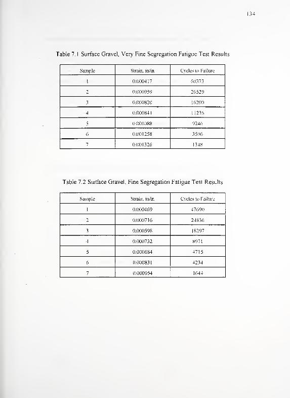
134
Table 7. 1 Surface Gravel, Very Fine Segregation Fatigue Test Results
Sample Strain, in/in Cycles to Failure
1 0.000417 60373
2 0.000959 26529
3 0.000820 16200
4 0.000841 1 1 236
5 0.001088 9246
6 0.001258 3506
7 0.001326 1348
Table 7.2 Surface Gravel, Fine Segregation Fatigue Test Results
Sample Strain, in/in Cycles to Failure
1 0.000469 47690
2 0.000716 24836
_> 0.000598 1 8297
4 0.000732 8971
5 0.000684 4715
6 0.000831 4234
7 0.000954 1644
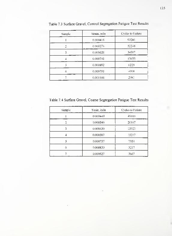
Table 7.3 Surface Gravel, Control Segregation Fatigue Test Results
Sample Strain, in/in Cvcles to Failure
1 0.000416 99280
2 0.000274 52248
3 0.000620 34507
4 0.000741 13033
5 0.000892 6229
6 0.000791 4068
7 0.001166 2981
Table 7.4 Surface Gravel, Coarse Segregation Fatigue Test Results
Sample Strain, in/in Cycles to Failure
1 000449 49100
2 0.000546 26107
3 0.000630 15923
4 0.000587 15217
5 0.000757 7351
6 0.000839 3217
7 0.000927 3867
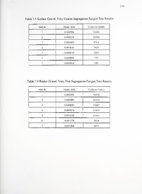
36
Table 7.5 Surface Gravel, Very Coarse Segregation Fatigue Test Results
Sample Strain, in/in Cycles to Failure
1 0.000384 32486
2 0.000435 25355
3 0.000469 8364
4 0.000610 3851
5 . 0.000644 3260
6 0.000898 737
7 0.000944 649
Table 7.6 Binder Gravel, Very Fine Segregation Fatigue Test Results
Sample Strain, in/in Cycles to Failure
1 0.000595 36696
2 0.000580 223 1
2
3 0.000820 1 9487
4 0.000974 1 249
1
5 0.001055 10561
6 0.001178 5818
7 0.001408 2876
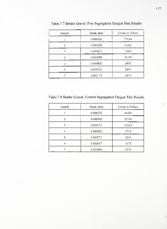
37
Table 7.7 Binder Gravel, Fine Segregation Fatigue Test Results
Sample .Strain, in/in Cycles lo Failure
1 0.000453 73744
-) 0.000528 21482
3 0.000611 13247
4 0.000698 10139
5 0.000820 5891
6 0.001012 2899
7 0.001173 1874
Sample Strain, in/in Cycles to Failure
1 0.000376 48950
2 0.000369 22741
3 0.000471 11615
4 0.000555 3715
5 0.000717 3216
6 0.000617 3073
7 0.001000 2375
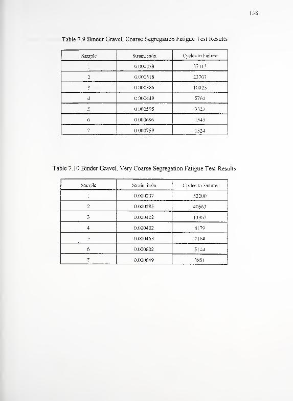
38
Table 7.9 Binder Gravel, Coarse Segregation Fatigue Test Results
Sample Strain, in/in Cycles lo Failure
1 0.000238 37113
2 0.000318 23767
3 0.000386 10025
4 0000449 5760
5 0.000595 3320
6 0.000696 1545
7 0.000759 1524
Table 7. 10 Binder Gravel, Very Coarse Segregation Fatigue Test Results
Sample Strain, in/in Cycles to Failure
1 0.000237 52200
2 0.000285 40563
:, 000402 13967
4 0.000462 8179
5 0.000463 7164
6 0.000602 5144
7 0.000649 385
1
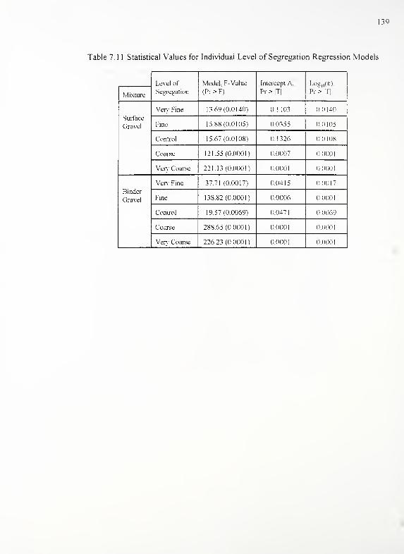
139
Level of
Segregation
Model. F-Value
(Pr>F)
Intercept A.
Pr > |T|
Logl0(e),
Pr > it;Mixture
Surface
Gravel
Very Fine 13.69(0.0140) 0.1103 0.0140
Fine 15.88(0.0105) 0.0355 0.0105
Control 15.67(0.0108) 0.1326 0.0108
Coarse 121.55(0.0001) 0.0007 0.0001
VeiT Coarse 221.13(0.0001) 0.0001 0.0001
Binder
Gravel
Very Fine 37.71 (0.0017) 0.0415 0.0017
Fine 138.82(0.0001) 0.0006 0.0001
Control 19.57(0.0069) 0.0471 0.0069
Coarse 288.65(0.0001) 0.0001 0.0001
Very Coarse 226.23 (0.0001) 0.0001 0.0001
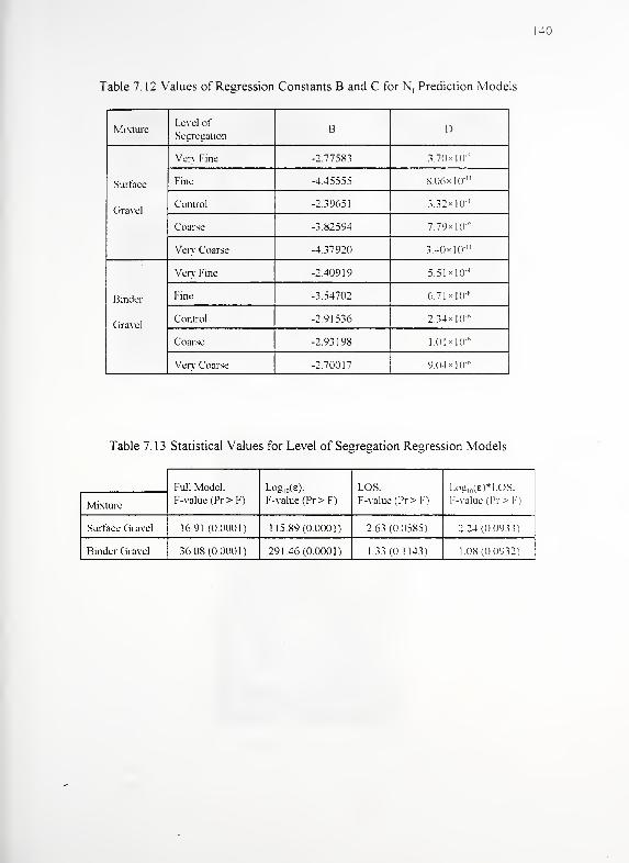
140
Table 7.12 Values of Regression Constants B and C for N, Prediction Models
MixtureLevel of
SegregationB I)
Surface
Ciravel
Ven Fine -2.77583 3.70*10"
Fine -4.45555 8 06* 10'"
Control -2.39651 3.32x10*'
Coarse -3.82594 7.79* 10"'
Ven Coarse -4.37920 3 40*10""
Binder
Gravel
Very Fine -2.40919 5.51 xIO*1
Fine -3.54702 6.71*K)-X
Control -2.91536 2.34* K)-"
Coarse -2.93198 1.01*Kr"
Ven' Coarse -2.70017 9()4*l(r"
Table 7.13 Statistical Values for Level of Segregation Regression Models
Full Model.
F-value (Pr > F)
Logio(e),
F-value (Pr > F)
LOS.
F-value (Pr>F)
I.og,„(£)*1.0S.
F-value (Pr> !•')
Mixture
Surface Gravel 16.91 (0.0001) 115.89(0.0001) 2.63 (0.0585) 2.24 (0.0933)
Binder Gravel 36.08(0.0001) 291.46(0.0001) 1.33(0.1143) 1 08(0.0932)
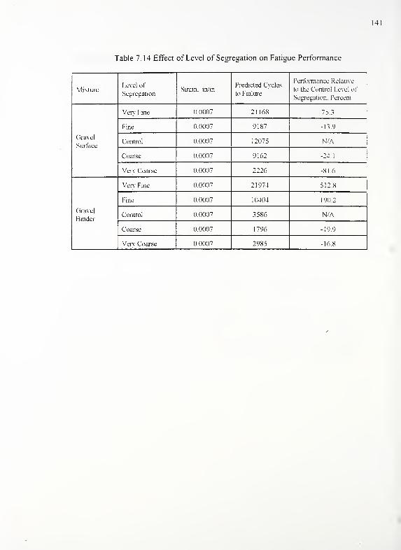
MixtureLevel of
SegregationStrain, in/in
Predicted Cycles
lo Failure
Performance Relative
lo the Control Level of
Segregation. Percent
Gravel
Surface
Very Fine 0.0007 21168 75.3
Fine 0.0007 9187 -13.9
Control 0.0007 12075 N/A
Coarse 0.0007 9162 -24.1
Very Coarse 0.0007 2226 -XI.
6
Gravel
Binder
Very Fine 0.0007 21974 512.8
Fine 0.0007 10404 190.2
Control 0.0007 3586 N/A
Coarse 0.0007 1 796 -49.9
Very Coarse 0.0007 2985 -16.8
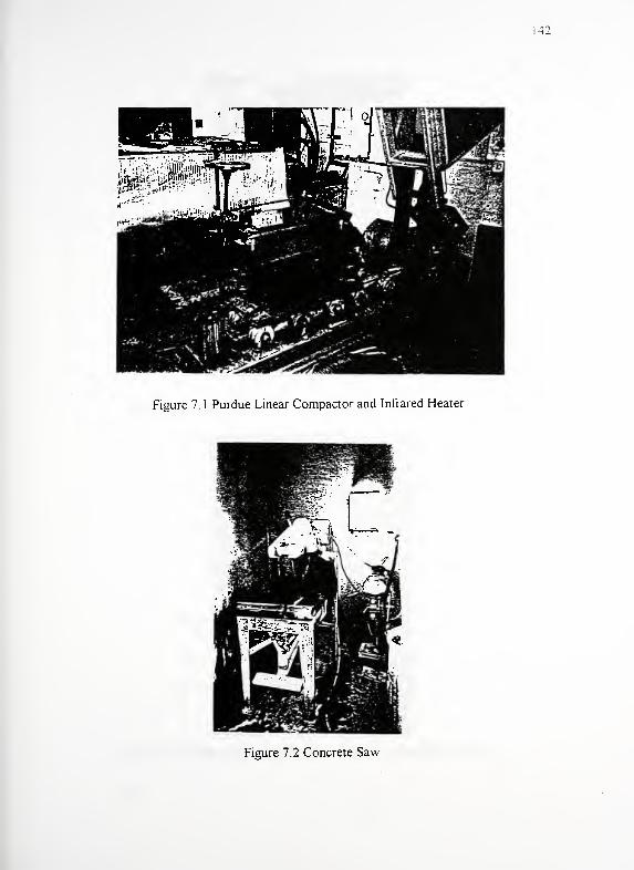
142
Figure 7.1 Purdue Linear Compactor and Infrared Heater
Figure 7.2 Concrete Saw
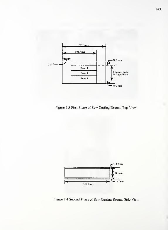
7mm— ^120.7 mm
501.7 mm
<r>
Beam 2
Beam 3
3 Beams, Each76.2 mm Wide
•38.1 mm
Figure 7.3 First Phase of Saw Cutting Beams, Top View
143
c12.7 mm
76.2 mm
381.0 mm•12 7 mm
Figure 7.4 Second Phase of Saw Cutting Beams, Side View
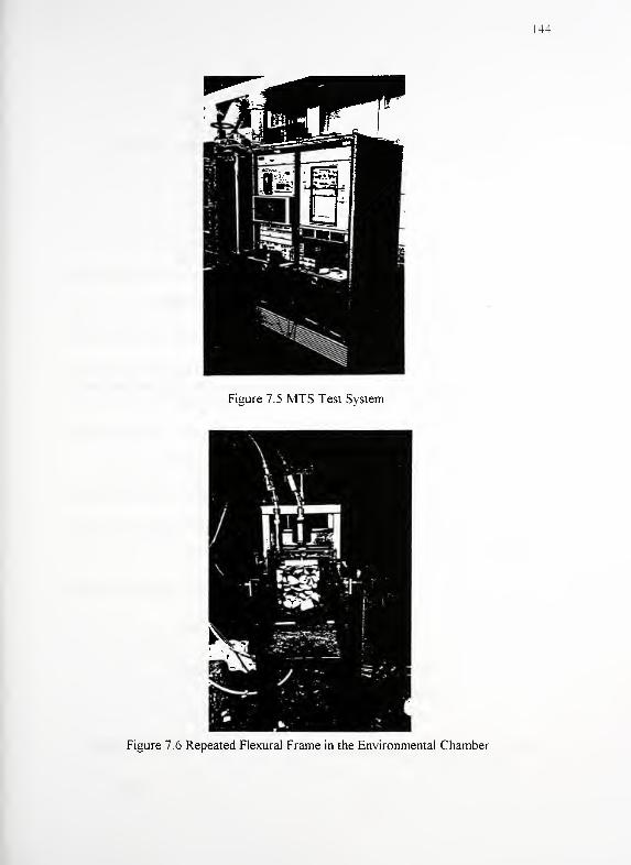
144
Figure 7.5 MTS Test System
Figure 7.6 Repeated Flexural Frame in the Environmental Chamber
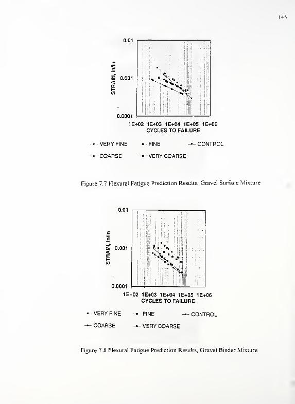
145
0.01
0.0001
1E+02 1E+03 1E+04 1E+05 1E+06CYCLES TO FAILURE
VERY FINE * FINE — CONTROL
-— COARSE — VERY COARSE
Figure 7.7 Flexural Fatigue Prediction Results, Gravel Surface Mixture
0.01
I 0.001<IX
0.0001
1E+02 1E+03 1E+04 1E+05 1E+06CYCLES TO FAILURE
VERY FINE • FINE -*- CONTROL
COARSE -*- VERY COARSE
p I Ifli'
i|j!lll|
;
; IHliftin?*;
jljjj••
>^W i'iT!
!
III
ill! i
i rw1
i
;
:i!1 hi
IP liSlll1
; :Hli
i
Fiuure 7.8 Flexural Fatigue Prediction Results, Gravel Binder Mixture
146
CHAPTER 8 LABORATORY ACCELERATED WHEEL TRACK TESTING
8.1 Introduction
In general, fatigue testing showed that the fine and very fine levels of segregation
performed better than the control mix and the coarse and very coarse levels of
segregation performed poorer. However, the fine level of segregation for the gravel
surface mixture did perform poorer than the control level of segregation. As a result, the
coarse levels of segregation would control to relative fatigue performance. For this
reason, laboratory wheel track device (WTD) tests were performed on the very coarse,
coarse, and control mixtures for both limestone and gravel mixtures.
Binder and surface mixtures for both aggregate types were tested with the WTD.
The characteristics of these mixtures were discussed in Chapter 4. The intent of this
testing was to determine the relative reduction in performance of coarsely segregated
mixtures due to wheel track testing in a hot, wet environment. The following discusses
the testing apparatus, sample preparation, test results and analysis.
8.2 Test Apparatus
8.2. 1 Purdue University Wheel Test Device
The Purdue University Wheel Test Device (PTD) was used for laboratory wheel
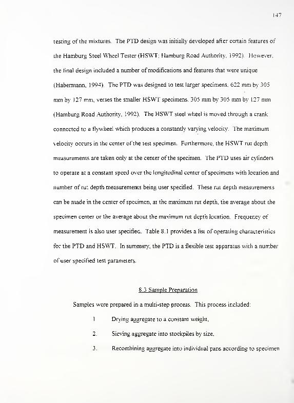
147
testing of the mixtures. The PTD design was initially developed after certain features of
the Hamburg Steel Wheel Tester (HSWT; Hamburg Road Authority, 1992). However,
the final design included a number of modifications and features that were unique
(Habermann, 1994). The PTD was designed to test larger specimens. 622 mm by 305
mm by 127 mm, verses the smaller HSWT specimens, 305 mm by 305 mm by 127 mm
(Hamburg Road Authority, 1992). The HSWT steel wheel is moved through a crank
connected to a flywheel which produces a constantly varying velocity. The maximum
velocity occurs in the center of the test specimen. Furthermore, the HSWT rut depth
measurements are taken only at the center of the specimen. The PTD uses air cylinders
to operate at a constant speed over the longitudinal center of specimens with location and
number of rut depth measurements being user specified. These rut depth measurements
can be made in the center of specimen, at the maximum rut depth, the average about the
specimen center or the average about the maximum rut depth location. Frequency of
measurement is also user specified. Table 8.1 provides a list of operating characteristics
for the PTD and HSWT. In summary, the PTD is a flexible test apparatus with a number
of user specified test parameters.
8.3 Sample Preparation
Samples were prepared in a multi-step process. This process included
1 Drying aggregate to a constant weight,
2. Sieving aggregate into stockpiles by size,
3. Recombining aggregate into individual pans according to specimen

148
gradation, density and asphalt content,
4. Heating combined aggregate and asphalt to the predetermined
mixing temperature based on asphalt viscosity,
5. Mixing aggregate and asphalt,
6. Curing mixture for approximately one hour,
7. Preheating the Purdue Linear Compactor (PLC) mold to the
compaction temperature using an infrared heater shown in Figure
8.1,
8. Compacting specimens with the PLC to the desired density and
thickness (approximately 38mm for surface and 51mm for binder
mixtures) as discussed in Chapter 4,
9. Allowing slabs to cool prior to removal from the PLC mold,
10. Measuring the slab heights at eight locations as shown in Figure
8.2 and then determine their weights,
1 1
.
Cutting samples in half using the concrete saw as previously
shown in Figure 6.2,
12. Placing the front half of the slab (relative to the PLC) in the right
side of the PTD, grouting the sample in place with plaster-of-paris
and then installing the back half of the slab in the left side of the
PTD in the same way.
After the plaster-of-paris cured (approximately 30 minutes), the PTD water reservoir was
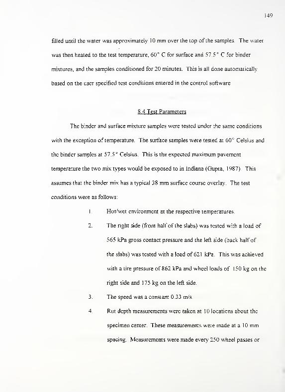
149
filled until the water was approximately 10 mm over the top of the samples. The water
was then heated to the test temperature, 60° C for surface and 57.5° C for binder
mixtures, and the samples conditioned for 20 minutes. This is all done automatically
based on the user specified test conditions entered in the control software
8.4 Test Parameters
The binder and surface mixture samples were tested under the same conditions
with the exception of temperature. The surface samples were tested at 60° Celsius and
the binder samples at 57.5° Celsius. This is the expected maximum pavement
temperature the two mix types would be exposed to in Indiana (Gupta, 1 987) This
assumes that the binder mix has a typical 38 mm surface course overlay The test
conditions were as follows:
1
.
Hot/wet environment at the respective temperatures
2. The right side (front half of the slabs) was tested with a load of
565 kPa gross contact pressure and the left side (back half of
the slabs) was tested with a load of 621 kPa. This was achieved
with a tire pressure of 862 kPa and wheel loads of 1 50 kg on the
right side and 175 kg on the left side.
3. The speed was a constant 0.33 m/s.
4. Rut depth measurements were taken at 1 locations about the
specimen center. These measurements were made at a 1 mm
spacing. Measurements were made every 250 wheel passes or
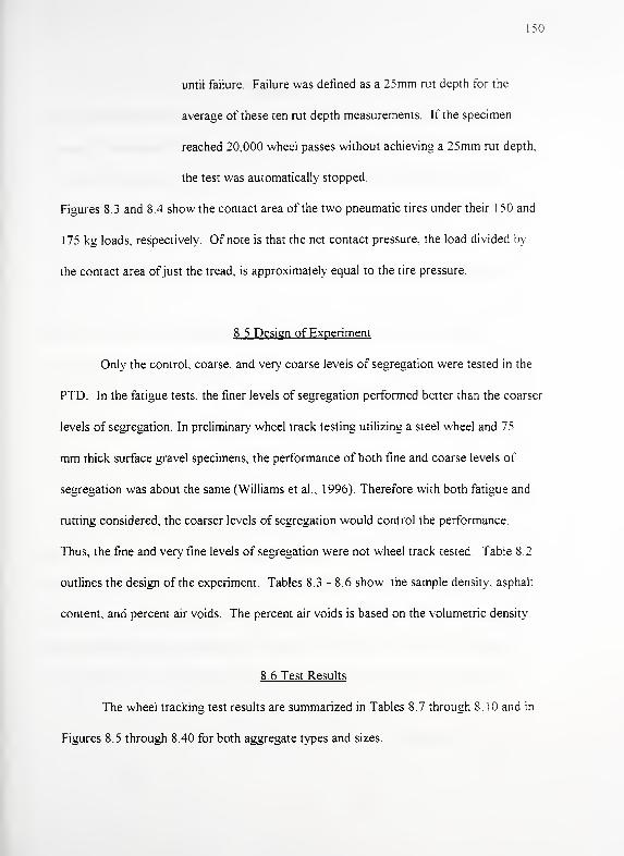
50
until failure. Failure was defined as a 25mm rut depth for the
average of these ten rut depth measurements. If the specimen
reached 20,000 wheel passes without achieving a 25mm rut depth,
the test was automatically stopped.
Figures 8.3 and 8.4 show the contact area of the two pneumatic tires under their 1 50 and
175 kg loads, respectively. Of note is that the net contact pressure, the load divided by
the contact area ofjust the tread, is approximately equal to the tire pressure
8.5 Design of Experiment
Only the control, coarse, and very coarse levels of segregation were tested in the
PTD. In the fatigue tests, the finer levels of segregation performed better than the coarser
levels of segregation. In preliminary wheel track testing utilizing a steel wheel and 75
mm thick surface gravel specimens, the performance of both fine and coarse levels of
segregation was about the same (Williams et al., 1996). Therefore with both fatigue and
rutting considered, the coarser levels of segregation would control the performance.
Thus, the fine and very fine levels of segregation were not wheel track tested Table 8.2
outlines the design of the experiment. Tables 8.3 - 8.6 show the sample density, asphalt
content, and percent air voids. The percent air voids is based on the volumetric density
8.6 Test Results
The wheel tracking test results are summarized in Tables 8.7 through 8.10 and in
Figures 8.5 through 8.40 for both aggregate types and sizes.
8.7 Analysis
Statistical analysis was performed on wheel track test data in a two-step process
The first step was defining the rate of deformation, creep and stripping rates. The second
step was statistically determining the effects of the test conditions and level of
segregation on mixtures.
The most basic result from wheel track testing is rate of deformation. Rate of
deformation is the final rut depth divided by the corresponding number of wheel passes
and is expressed as mm per wheel pass (mm/wp).
Creep rate is the rate at which a slab experiences permanent deformation without
the compounding effect of moisture. This is best represented in Figure 8.5, where both
specimens tested at 621 and 565 kPa experienced pure creep. Thus, the creep rate is the
deformation due to creep of a specimen divided by the number of wheel passes Creep
rates were statistically determined by best fit of the data with respect to linear regression
analysis
Stripping rate is defined similar to creep rate. Figure 8.29 shows two samples
tested at 621 and 565 kPa contact pressure, respectively, that demonstrate pure stripping
The best fit linear regression equation of data defined the stripping rates. Like creep rate,
stripping rate is the rate of deformation when stripping occurs and is expressed as mm of
rut depth per wheel pass. Tables 8.7 through 8.10 summarize rate of deformation, creep
and stripping rates, and stripping inflection points for test samples. The intersection of
the creep and stripping slopes is referred to as the stripping inflection point
The second step in statistical analysis of wheel track test data was performing
analysis of variance (ANOVA) using SAS (SAS Institute, 1991 ). The following equation
represents the split-plot design used to examine the rate of deformation, creep and
stripping rates.
Y = u + LOS, + CP,+ LOS(SAM)I(10
+ LOS><CP,, + CP*LOS(SAM)„(k)+ Error (
1
)
where:
Y = Rate of Deformation, Creep Rate, Stripping Rate, Stripping
Inflection Point
LOS = Level of Segregation (control, coarse, very coarse),
CP = Contact Pressure (565 kPa, 621 kPa), and
SAM = Sample (1,2,3 9).
The LOS(SAM)lkterm was used as the error term to test the level of segregation, LOS,,
for statistical significance. The CP*LOS(SAM)ij(k)
term was used as the error term to test
the contact pressure, CP,, and the interaction term between level of segregation and
contact pressure, LOS*CPij
, for statistical significance. The results of the analyses are
summarized in Tables 8.11 through 8.13.
8.7.1 Gravel Surface Mixture
Data for gravel surface mixture data included of rate of deformation, creep and
stripping rates, and stripping inflections. Of the samples tested, more than half did not
experience stripping. No analysis for the stripping rates and stripping inflection points
were performed because of the limited samples size per test cells.
The rate of deformation ANOVA shows that only the contact pressure is
significant for an alpha = 5 percent. The average rate of deformation for samples tested
with the 565 and 621 kPa contact pressures were 0.00037422 and 0.00052144 mm per
wheel pass, respectively. A sample tested with a higher contact pressure would be
expected to have a higher rate of deformation than a lower contact pressure. ANOVA of
the creep rate shows none of the variables to be statistically significant
8.7.2 Limestone Surface Mixture
Data for the limestone surface mixture included rate of deformation, creep and
stripping rates, and stripping inflection points. Like the gravel surface mixture, the
limestone surface mixture had limited sample size per cell for stripping rates and
stripping inflection points. Thus, no analysis for stripping rate was performed.
The rate of deformation ANOVA shows the contact pressure and the interaction
between the level of segregation and contact pressure to be significant for an alpha = 5
percent. The level of segregation was significant for an alpha - 7 percent. The mean rate
of deformation for the control, coarse, and very coarse levels were 0020697,
0.0001892, 0.0003990 mm of rut depth per wheel pass, respectively The coarse and
very coarse levels of segregation performed better than the control mix which was not
expected. One explanation of this result is that for the gradation, the selected optimum
154
asphalt content was low. Consequently, there was insufficient asphalt coating of the finer
material in the control mix. This would make the control mix more susceptible to
moisture damage or stripping. Every control sample did experience stripping
The average rate of deformation for the 565 and 621 kPa contact pressures were
0.0007022 and 0.001 0697 mm of rut depth per wheel pass, respectively. Like the gravel
surface mixture, higher contact pressure produced a higher rate of deformation.
ANOVA of the creep rate data found the contact pressure and the interaction
between the level of segregation and contact pressure to be significant for alpha = 5
percent. The average creep rates for the 565 and 621 kPa contact pressures were
0.0007022 and 0.0010697 mm of rut depth per wheel pass, respectively. As expected,
higher contact pressure yielded a higher creep rate.
8.7.3 Gravel Binder Mixture
Data for the gravel binder mixture data consisted of rate of deformation, creep
rates, and stripping rates, and stripping inflection points. A few of the samples did not
experience creep and stripping, thus not all of the cell sample sizes are equal
ANOVA of the rate of deformation and creep rates found none of the variables to
be statistically significant for alpha = 5 percent. This indicates that the gravel mixtures
are very susceptible to stripping/rutting. It is a characteristic of the gravel, i.e. rounded,
low crushed faces or mineralogical.
ANOVA of the stripping rate found the level of segregation was significant at
higher than alpha = 5 percent. The average rate of stripping for the very coarse level was
155
0.043 166 mm of rut depth per wheel pass while that of the coarse and control levels were
0.004201 and 0.0041 15 mm of rut depth per wheel pass, respectively. This indicates that
coarsely segregated mixtures are sensitive to moisture once failure begins. Analysis of
the stripping inflection points yielded a model with an F-value of 2.18, showing that use
of stripping inflection points is not appropriate in evaluating mixtures.
8.7.4 Limestone Binder Mixture
Data for the limestone binder mixture data consisted of rate of deformation and
creep rates for nearly all samples tested. The sample sizes within the test cell were
unbalanced for the creep rate data because two of the samples did not experience creep
Like the surface mixtures, the limestone binder mixture had very low samples sizes
within the test cells for the stripping rate and stripping inflection points. Thus. ANOVA
was not performed for the stripping rates and stripping inflection points
ANOVA of the rate of deformation found the level of segregation was the only
statistically significant variable at alpha = 8 percent. ANOVA of the creep rates found no
significant variables. The lack of significance with the contact pressure was not expected
because at the control and coarse levels of segregation, exclusivity of failure did not
occur at the higher 621 kPa contact pressure. This resulted in very slight differences in
the performance at the control and coarse levels of segregation.
The effect of level of segregation on the performance of a mixture due to wheel
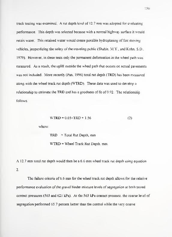
156
track testing was examined. A ait depth level of 12.7 mm was adopted for evaluating
performance. This depth was selected because with a normal highway surface it would
retain water. This retained water would create possible hydroplaning of fast moving
vehicles, jeopardizing the safety of the traveling public (Shahin, MY., and Kohn. S.D.,
1 979). However, in these tests only the permanent deformation in the wheel path was
measured. As a result, the uplift outside the wheel path that occurs on actual pavements
was not included. More recently (Pan, 1996) total rut depth (TRD) has been measured
along with the wheel track rut depth (WTRD). These data was used to develop a
relationship to estimate the TRD and has a goodness of fit of 0.92. The relationship
follows.
WTRD = 65xTRD+ 1.56 (2)
where:
TRD = Total Rut Depth, mm
WTRD = Wheel Track Rut Depth, mm.
A 12.7 mm total rut depth would then be a 6.6 mm wheel track rut depth using equation
2.
The failure criteria of 6.6 mm for the wheel track rut depth allows for the relative
performance evaluation of the gravel binder mixture levels of segregation at both tested
contact pressures (565 and 621 kPa). At the 565 kPa contact pressure, the coarse level of
segregation performed 65.7 percent better than the control while the very coarse

57
performed 49.0 percent poorer than the control. Similar performance resulted with the
621 kPa contact pressure. The coarse level of segregation performed 48.9 percent better
than the control mixture at the 565 kPa contact pressure while the very coarse level of
segregation performed 73.3 percent poorer than the control under the 621 kPa.
Examination of the performance between the two contact pressures at different levels of
segregation for the gravel binder mixture shows the higher contact pressure causes
progressively poorer performance with coarser segregation. The 621 kPa versus the 565
kPa contact pressure resulted in a reduction in performance of 34.6, 41 .2, and 65.8
percent for the control, coarse, and very coarse levels of segregation, respectively. These
results are summarized in Table 8.14.
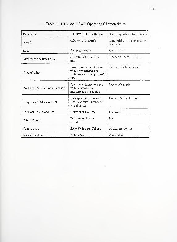
58
Table 8.1 PTD and HSWT Operating Characteristics
Parameter PURWheel Test Device Hamburg Wheel Track Tester
Speed0.20 m/s to 0.40 m/s Sinusoidal with a maximum of
33 m/s
Load 500 N to 1 900 N Up to 697 N
Maximum Specimen Size622 mm* 305 mm* 127
mm305 mmx.lOS nun* 1 27 mm
Type of Wheel
Steel wheel up to 1 00 mmwide or pneumatic tire
with tire pressure up to 862
kPa
47 mm wide Steel w heel
Rut Depth Measurement Location
Anywhere along specimen
with the number of
measurements specified
Center of sample
Frequency of Measurement
User specified, from every
1 to maximum number of
wheel passes
Every 250 wheel passes
Environmental Condition Hot/Wet or Hot/Dry I lot/Wet
Wheel WanderDistribution is user
specified
No
Temperature 25 to 60 degrees Celsius 50 degrees Celsius
Data Collection Automated Automated
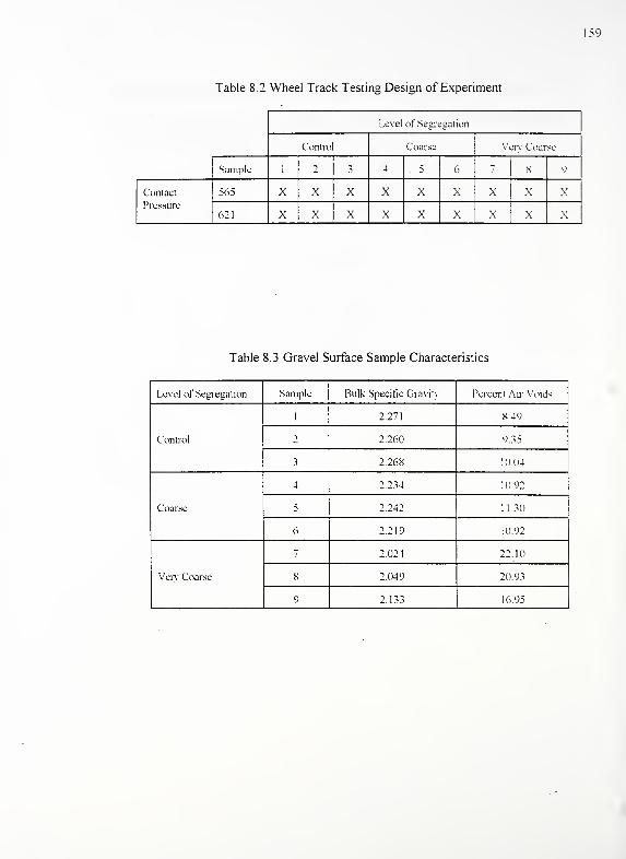
Table 8.2 Wheel Track Testing Design of Experiment
Table 8.3 Gravel Surface Sample Characteristics
159
Level of Segregation
Control Course Very Coarse
Sample 1 2 3 4 5 6-
X ')
Contact
Pressure
565 X X X X X X X X X
621 X X X X X X X X X
Level of Segregation Sample Bulk Specific Gravity Percent Air Voids
Control
1 2.271 8 49
2 2.260 9.35
3 2.268 10 04
Coarse
4 2.234 10 92
5 2.242 11.30
6 2.219 10.92
Veiy Coarse
7 2.024 22.10
8 2.049 20.93
9 2.133 16 95
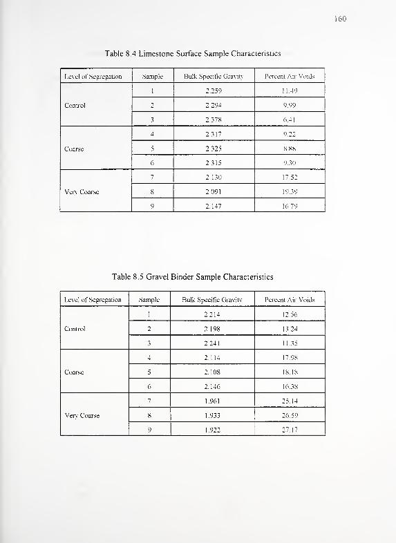
160
Table 8 4 Limestone Surface Sample Characteristics
Level of Segregation Sample Bulk Specifie Gravity Percent Air Voids
Control
1 2.259 1 1 49
i 2.294 9 99
3 2.378 6.4]
Coarse
4 2.317 9.22
5 2.325 SX8
6 2.315 9 30
Veiy Coarse
7 2.130 17 52
8 2.091 19,39
9 2.147 16 79
Table 8.5 Gravel Binder Sample Characteristics
Level of Segregation Sample Bulk Specific Gravity Percent Air Voids
Control
1 2.214 12.56
2 2.198 13.24
3 2.241 1 1 .35
Coarse
4 2.114 17.98
5 2.108 18 18
6 2.146 16.38
Ven' Coarse
7 1.961 25.14
8 1.933 26.59
9 1.922 27.17
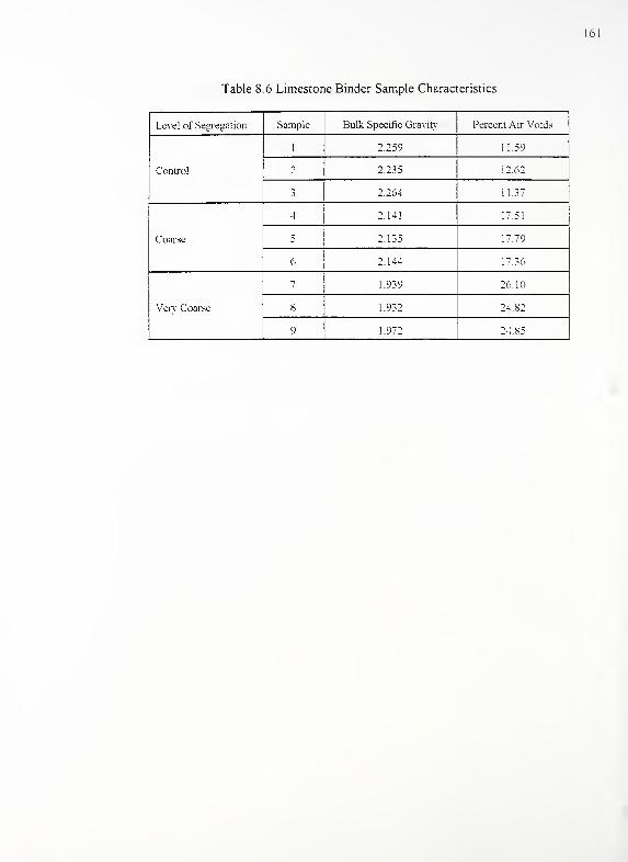
Table 8.6 Limestone Binder Sample Characteristics
161
Level of Segregation Sample Bulk Specific Gravity Percent Air Voids
Control
1 2.259 11.59
2 2.235 12.62
3 2.264 11.37
Coarse
4 2.141 17.51
5 2.135 17.79
6 2.144 17.36
Very Coarse
7 1.939 26.10
8 1.932 24.82
9 1.972 24.85
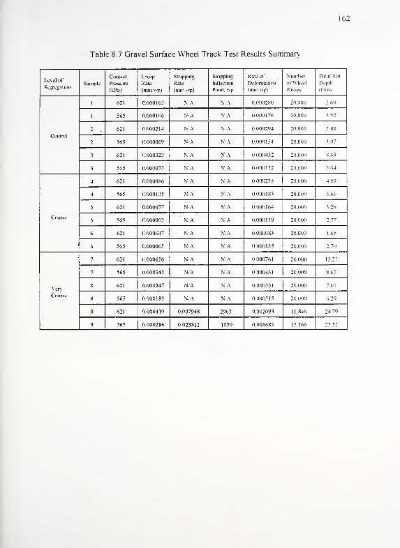
Table 8.7 Gravel Surface Wheel Track Test Results Summary
162
Level of
SegregationSample
Contact
Pressure
(kl>a)
Creep
Kale
(mm wp)
Stripping
Rate
(mnvwp)
Stripping
Inflection
Point, wp
Rate of
Deformation
(mm wp)
Numberol Wheel
Passes
1 ni.il KmDepth
(mnii
Control
1 621 0.000163 N A N A 0.0002X0 20.000 5.60
1 565 0.000106 N A N A 0,000176 20.000 3.52
2 621 0.000214 N A \ A 0.000294 20.000 5 XX
2 565 0.000069 N/A N A 0.000154 20.000 3 07
3 621 0.000323 N A N A 0,000432 20.000 X.f.3
3 565 0.000073 N A N A 0.000152 20.000 3.04
Coarse
4 621 0.0000X6 N/A N A 0.000235 20.000 4.69
4 565 0.000135 N/A N A 0.000183 20.000 3,66
5 621 0.000077 N/A N A 0.000164 20.000 3.2X
5 565 0.000063 N A N A 0.000139 20.000 2,77
6 621 0.000037 N A N/A 0.0000X3 20.000 1.65
6 565 0.000065 N/A N A 0.000135 20.000 2.70
YenCoarse
7 621 0.000656 N/A N/A 0.000761 20.000 15.21
7 565 0.000341 N/A N A 0.000431 20.000 X.62
X 621 0.000247 N/A N A 0.000351 20.000 7 01
X 565 0.000185 N/A N A 0.0003 1 5 20.000 6.29
9 621 0.000419 0.007948 2963 0.002093 1 1 .846 24 79
9 565 0000286 0.023811 1059 0.0016X3 15.166 25.52
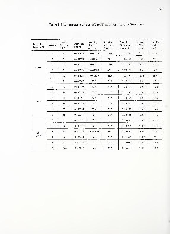
Table 8 8 Limestone Surface Wheel Track Test Results Summary
163
Level of
SegregationSample
Contact
Pressure
(kPa)
Creep Rate
(nmvwp)
Stripping
Rale
(mnvwp)
Stripping
Inflection
Point, wp
Rate of
Deformation
(mm wp)
Numberof Wheel
Passes
Final Rut
Depth
(mm)
C omrol
1 621 0.002154 0.007280 2636 0.004424 5.622 24.X7
1 565 001698 0.007161 2883 0.002906 8.7X8 25 54
2 621 0.000723 007143 3210 0.002020 12.500 25.25
2 565 0.000333 0.002988 4231 0.000675 20.000 14 05
3 621 0.000535 0.010850 2226 0.001987 12.750 25.34
3 565 0.000247 N A N A 0.000406 20.000 8.12
C oarse
4 621 0.000049 N A N A 0.000164 20.000 3.28
4 565 0.000154 N A N A 0000230 20.000 4.59
5 621 0.000091 N A \ A 0.000170 20.000 3.06
5 565 0.000052 N A N A 0.000243 20.000 4.3S
6 621 0.000084 N A N A 0.000170 20.000 3.40
6 565 0.000075 N A N A 000158 20.000 3.16
YenCoarse
7 621 0.000152 N A N A 0.000221 20.000 4.41
7 565 0.000145 N A X A 0.000229 20.000 4.58
8 621 0.000250 0.005639 4344 0.000388 1 8.650 25.58
X 565 0.000264 N A N A 0.001372 20.000 "5
9 621 0.000027 N A N A 0.000084 20.000 1.6"
9 565 0.000040 N A N A 0.000101 20.001) 2.02
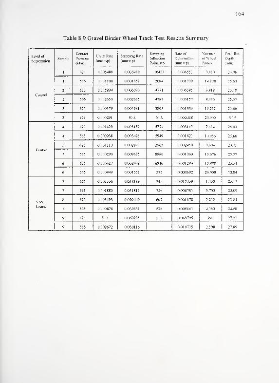
Table 8.9 Gravel Binder Wheel Track Test Results Summary
164
Level of
SegregationSample
Contact
Pressure
(kPa)
Creep Rate
(nun wp)
Stripping Rate
(mm up)
Stripping
Inflection
Point, ivp
Rale ol'
Delomiation
(nun up)
Number
ol Wheel
Passes
1 mal Rut
Depth
(mini
C onlrol
1 621 0.005488 0.005488 10453 0.006551 3.810 24.96
1 565 0.001100 0.001352 2084 0.001739 14.29X 25.63
2 621 0.005994 0.006090 4771 0.006595 3.818 25. IX
2 565 0.002653 0.002665 4787 0.003157 X.036 25.37
3 621 0.000379 0.004981 3803 0.001336 1 9.2 1
2
25.66
3 565 0.000291 N A N A 0.000408 20.000 K.I 5
C oarse
4 621 0.001429 0.005 1 52 5774 0.003163 7.914 25 03
4 565 0.000938 0.003496 5949 0.001821 14.056 25.60
5 621 0.001113 0.002879 2565 0.002450 9.694 23.7?
5 565 0.000293 0.009675 8880 0.001300 1 9.676 25.57
6 621 0.000427 0.002449 6916 0.0012X4 19.XXX 25.54
6 565 0.000449 0.001552 575 0.000692 20.000 13.84
YenCoarse
7 621 0.005556 0.038189 745 0.017359 1 .450 25. 1
7
7 565 0.001880 0.031813 724 0.0067X1 3.700 25.09
X 621 0.003493 0.029449 607 0.001078 2.212 23.84
X 565 0.000878 0.03963
1
528 0.005651 4.350 24.58
9 621 N.-\ 0.069795 NA 0.069795 390 27.22
9 565 0.002672 0.050116 0.010735 2.59X • 27.89
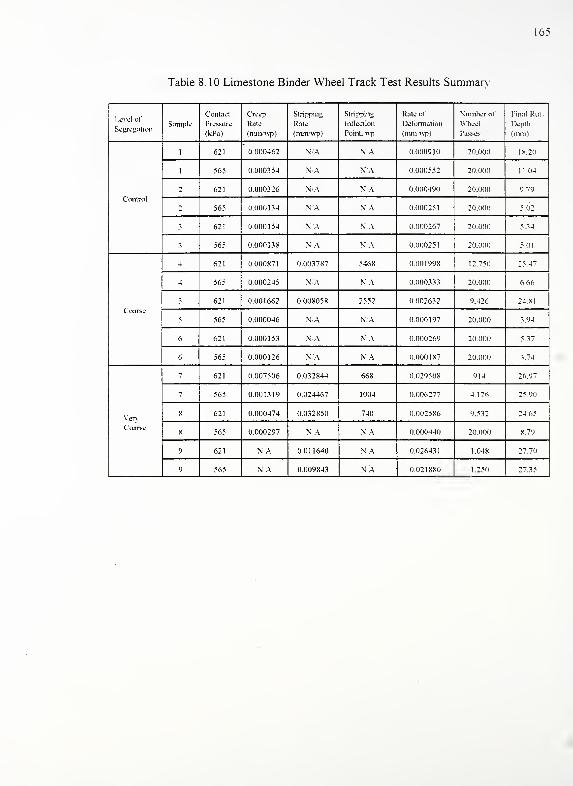
Table 8. 10 Limestone Binder Wheel Track Test Results Summary
165
] .ovel of
SegregationSample
Contact
Pressure
(kPa)
Creep
Rate
(mm \vp)
Stripping
Rate
(mni'\vp)
Stripping
Inflection
Point. \vp
Rate of
Deformation
(mm up)
Number of
Wheel
Passes
l-'inal KmDepth
(mm)
Control
1 621 0.000462 N A N/A 0.000910 20.000 18.20
1 565 0.000354 N A N A 0.000552 20.000 11.04
2 621 0.000326 N/A N A 0.000490 20.000 9.79
2 565 0.000134 N A N A 0.000251 20.000 5.02
3 621 0.000154 N A N/A 0.000267 20.000 5 34
3 565 0.000138 N A N A 0.000251 20.000 5.01
Coarse
4 621 0.000871 0.003787 5468 0.001998 12.750 25 4"
4 565 0.000245 N/A N A 0.000333 20.000 6 66
5 621 0.001662 0.008058 2552 0.002632 9.426 24 81
5 565 0.000046 N/A N/A 0.000197 20.000 3 94
6 621 0.000153 N/A N A 0.000269 20.000 5.37
6 565 0.000126 N A N/A 0.000187 20.000 3.74
Verv
Coarse
7 621 0.007506 0.032844 668 0.029508 914 26.97
7 565 0.001319 0.024467 1004 0.006277 4.126 25.90
X 621 0.000474 0.032850 740 0.002586 9.532 24 65
X 565 0.000297 N A N/A 0.000440 20.000 8.79
9 621 N/A 0.011640 N A 0.026431 1.048 27.70
9 565 N A 0.009843 N/A 0.021880 1.250 27.35
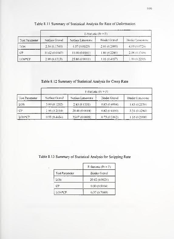
166
Table 8.1 1 Summary of Statistical Analysis for Rate of Deformation
F-Statistic (Pr > F)
Test Parameter Surface Gravel Surface Limestone Binder Grave] Binder Limestone
[.OS 2.36(0.1749) 4.57 (0.0623) 2.06 (0.2089) 4 19(0.0728)
CP 11.62(0.0143) 1 1.00(0.0161) 1 .80 (0.2286) 2.98(0.1348)
LOS*CP 2.90(0.1313) 25.86(0.0011) 1.05(0.4057) 1.90(0.2295)
Table 8. 12 Summary of Statistical Analysis for Creep Rate
F-Statistic (Pr> F)
Test Parameter Surface Gravel Surface Limestone Binder Gravel Binder Limestone
LOS 3.00(0.1252) 2.85(0.1351) 0.83 (0.4994) 1 83 (0.2530)
CP 1 96(0.2114) 28.48(0.0018) 0.82(0.4160) 3.31 (0.1284)
LOS*CP 0.93 (0 4454) 35.07 (0.0005) 0.73 (0.5362) 1.55(0.2998)
Table 8.13 Summary of Statistical Analysis for Stripping Rate
F-Statistic (Pr > F)
Test Parameter Binder Gravel
LOS 20.42(0.0021)
CP 0.50(0.5104)
LOS*CP 0.37 (0.7089)
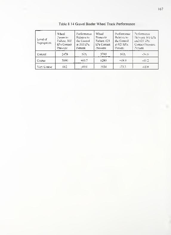
167
Table 8 14 Gravel Binder Wheel Track Performance
Level of
Segregation
Wheel
Passes to
Failure. 565
kPa Contact
Pressure
Performance
Relative to
the Control
at 565 kPa.
Percent
Wheel
Passes to
Failure. 62
1
kPa Contacl
Pressure
Performance
Relative to
the Control
at 621 kPa.
Percent
Performance
Between 565 kl'a
and 62 1 kl'a
Contact Pressure.
Percent
Control 2478 N/A 3789 N/A -34.6
Coarse 3690 +65.7 6280 +48.9 -41.2
Veiy Coarse 662 -49.0 1934 -73.3 -65. X
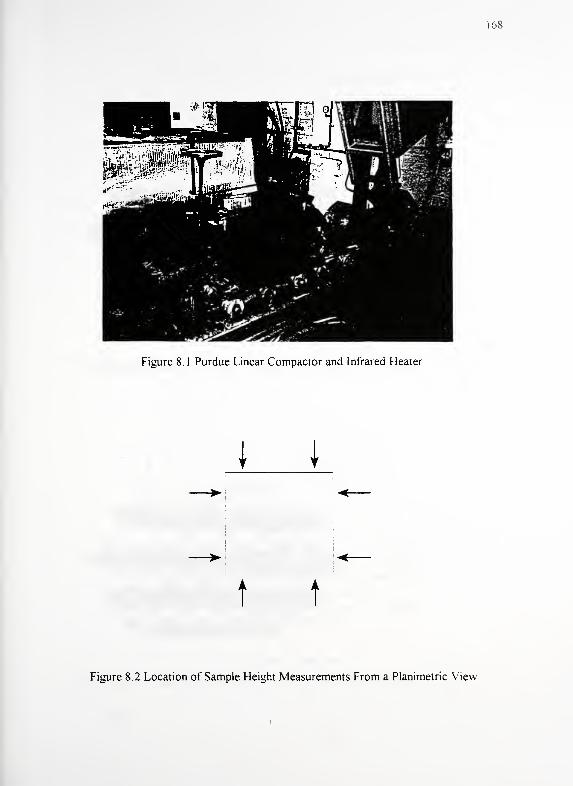
168
Figure 8.1 Purdue Linear Compactor and Infrared Heater
\ I
t t
Figure 8.2 Location of Sample Height Measurements From a Planimetric View
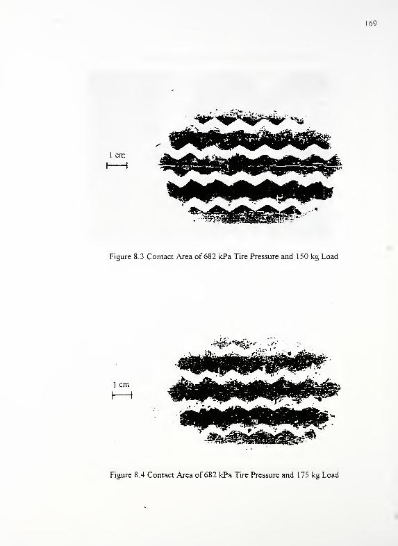
169
cm
I 1
Figure 8.3 Contact Area of 682 kPa Tire Pressure and 150 k" Load
1 cm
Figure 8.4 Contact Area of 682 kPa Tire Pressure and 175 k" Load
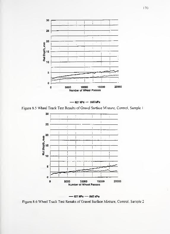
170
30
25
20
Q.15aa
10
5000 10000 15000
Number of Wheel Passes
20000
— 621 kPa— 565 kPa
Figure 8.5 Wheel Track Test Results of Gravel Surface Mixture, Control, Sample
30 1!
25
20E !
E
10
! ! i !^
! ! I
I ]' I! I
! !I
i
i | j |
! |j | j L_^|
i
_ ^^^==ZZClZ^_^-\-^"T^T
1""
!
i ; i i
5000 10000 15000 20000
Number of Wheel Passes
— 621 kPa— 565 kPa
Figure 8.6 Wheel Track Test Results of Gravel Surface Mixture, Control, Sample 2
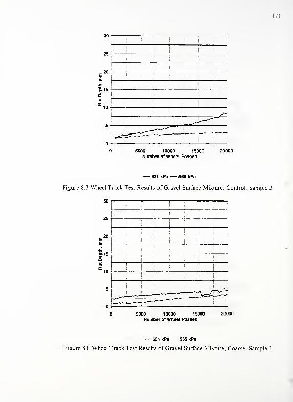
171
30
25
20
Q.15
5000 10000 15000 20000Number of Wheel Passes
— 621 kPa— 565 kPa
Figure 8 7 Wheel Track Test Results of Gravel Surface Mixture, Control. Sample 3
30
25
20
1-15
10
7— — "*^
5000 10000 15000 20000
Number of Wheel Passes
— 621 kPa— 565 kPa
Figure 8.8 Wheel Track Test Results of Gravel Surface Mixture, Coarse, Sample l
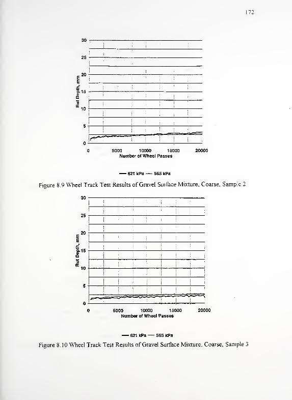
172
30
25
20
a.15
10
5
5000 10000 15000 20000Number of Wheel Passes
621 kPa— 565 kPa
Figure 8.9 Wheel Track Test Results of Gravel Surface Mixture, Coarse, Sample 2
30 -; :
25
20
a.15
5000 10000 15000 20000
Number of Wheel Passes
— 621 kPa— 565 kPa
Figure 8.10 Wheel Track Test Results of Gravel Surface Mixture, Coarse, Sample 3
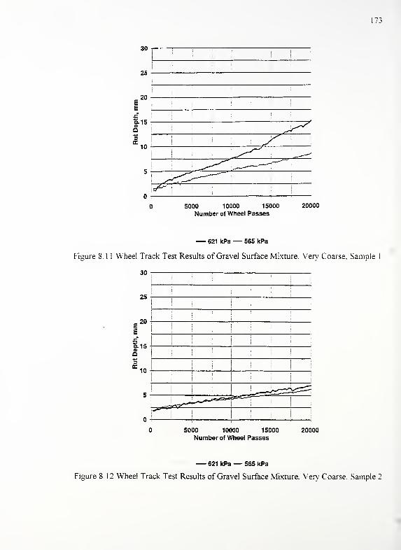
173
30
25
E20
E
I 15
o
10
**i
5000 10000 15000
Number of Wheel Passes20000
— 621 kPa— 565 kPa
Figure 8. 1 1 Wheel Track Test Results of Gravel Surface Mixture, Very Coarse. Sample
30
25
e20
;
E
e-15
5000 10000 15000 20000
Number of Wheel Passes
— 621 kPa— 565 kPa
Figure 8.12 Wheel Track Test Results of Gravel Surface Mixture, Very Coarse. Sample 2
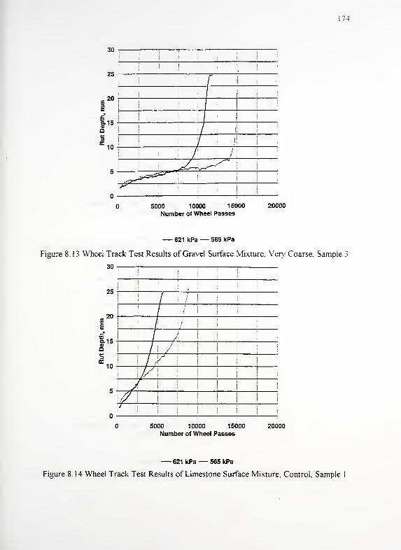
174
30
25
E20
E
so
10
iI
i
'
iI !
I . ,
1
ri
I i
:/
| 1
1/ i
/ ''
! /' /
^~^^'^^^^
'^!
5000 10000 15000
Number of Wheel Passes
20000
— 621 kPa— 565 kPa
Figure 8.13 Wheel Track Test Results of Gravel Surface Mixture, Very Coarse. Sample 3
30
25
20 f
Q.15a>
a
10
I I
;
I !
; fill/ ''
'
f U
/ ^i
\ J II
! 1 / i
i 1 1 i
1 is i
!
i i
i i
X// ! I
ii 1
5000 10000 15000 20000
Number of Wheel Passes
— 621 kPa— 565 kPa
Figure 8.14 Wheel Track Test Results of Limestone Surface Mixture, Control. Sample
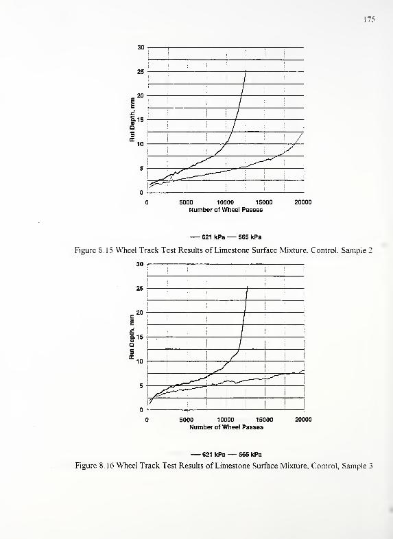
175
30
25
20
9-15
10
i
i!
I
;
I
i
/
; /
j J|/
/ // : >
^f 1^-f.I J^rC^-^r
—"^
i^-T'i
i
5000 10000 15000 20000
Number of Wheel Passes
— 621 kPa— 565 kPa
Figure 8. 15 Wheel Track Test Results of Limestone Surface Mixture. Control, Sample 2
30 i
i
10i
1 1/ !
I
I
1/ I I I.J
; ^cp-r^i\f | 1 ! |
! !
'
1:
' ^—^^—^^—
5000 10000 15000 20000
Number of Wheel Passes
— 621 kPa— 565 kPa
Figure 8. 16 Wheel Track Test Results of Limestone Surface Mixture, Control, Sample 3
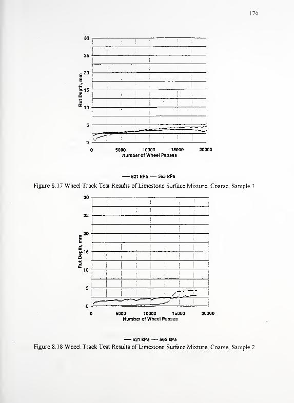
76
30
25
E20
EJB
a.154)
Q
= 10
5000 10000 15000
Number of Wheel Passes
20000
— 621 kPa— 565 kPa
Figure 8.17 Wheel Track Test Results of Limestone Surface Mixture, Coarse. Sample 1
30
25
E20
E
oa i i
!
i i
i j
10
! ! i
i
!
! i I
'
! S .. .ii! "L -
5000 10000 15000
Number of Wheel Passes20000
— 621 kPa— 565 kPa
Figure 8.18 Wheel Track Test Results of Limestone Surface Mixture, Coarse. Sample 2
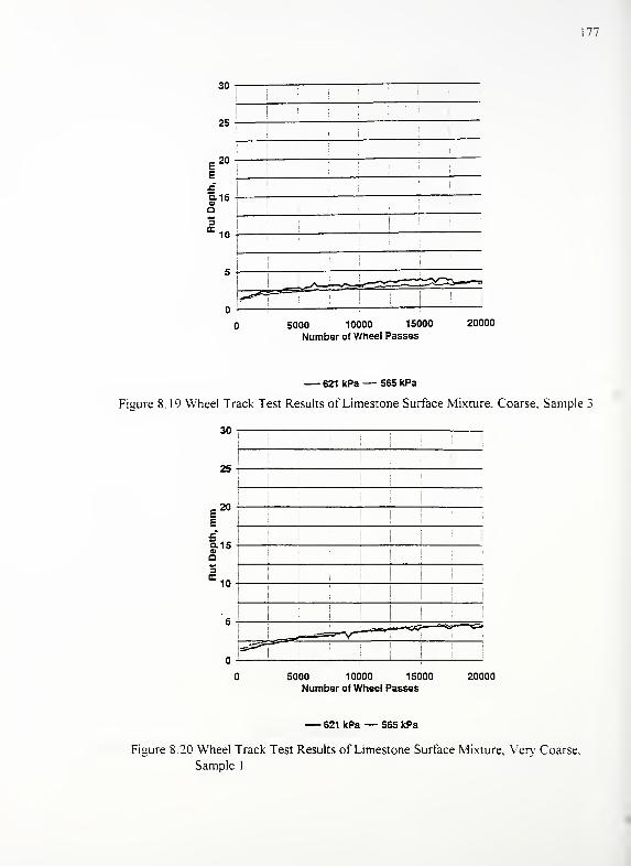
30
25
20
e-is
10
1 77
5000 10000 15000
Number of Wheel Passes
20000
— 621 kPa— 565 kPa
Figure 8. 19 Wheel Track Test Results of Limestone Surface Mixture. Coarse, Sample 3
30 ;;
25
20
S-15a
10
5000 10000 15000
Number of Wheel Passes20000
— 621 kPa— 565 kPa
Figure 8.20 Wheel Track Test Results of Limestone Surface Mixture, Very Coarse,
Sample l
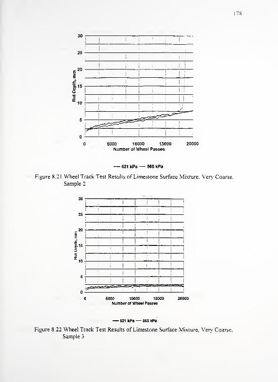
78
30
25
E20
EJC
Q.150)
Q
10
! 'i
Ii
j
I
i
i!
'
I
i
| illI !
i':
I
|i ; I
_/ ,_!
^^-?cs^;
^^^^^^^I
r i
i
ii
. ii
i
5000 10000 15000 20000
Number of Wheel Passes
— 621 kPa — 565 kPa
Figure 8.21 Wheel Track Test Results of Limestone Surface Mixture, Very Coarse.
Sample 2
30
25
20
3-15
10
5000 10000 15000 20000
Number of Wheel Passes
621kPa— 565 kPa
Figure 8.22 Wheel Track Test Results of Limestone Surface Mixture, Very Coarse,
Sample 3
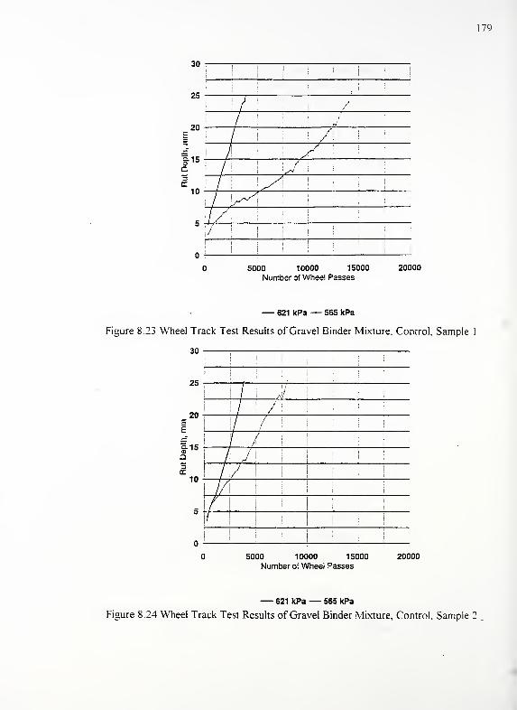
179
oui
• ;i
25/ /
20E
J!
i'
/: /
I 15
Q
1/I
! /I 'W i
1
3cc
10/
j ^y 1 ,]
: / \^-y
5//1 / !
;/'
i
:
ni
!
!
5000 10000 15000 20000
Number of Wheel Passes
— 621 kPa— 565 kPa
Figure 8.23 Wheel Track Test Results of Gravel Binder Mixture, Control, Sample
30
5000 10000 15000 20000Number of Wheel Passes
— 621 kPa— 565 kPa
Figure 8.24 Wheel Track Test Results of Gravel Binder Mixture, Control, Sample
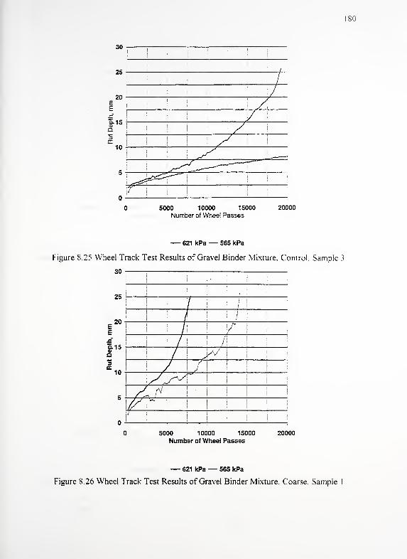
30
5000 10000 15000 20000
Number of Wheel Passes
— 621 kPa— 565 kPa
Figure 8.25 Wheel Track Test Results of Gravel Binder Mixture. Control. Sample
5000 10000 15000Number of Wheel Passes
Depth,
mm
-»
to
ro
o
en
o
in
c
'
i
/ !
//
/
V ! :
,/ :
/ W= 10-
J I f I
I
! I
\yif^r5 - Af< i
'!
iI
/:w
| j
'
«
/j
I |I
20000
— 621 kPa— 565 kPa
Figure 8.26 Wheel Track Test Results of Gravel Binder Mixture, Coarse, Sample I
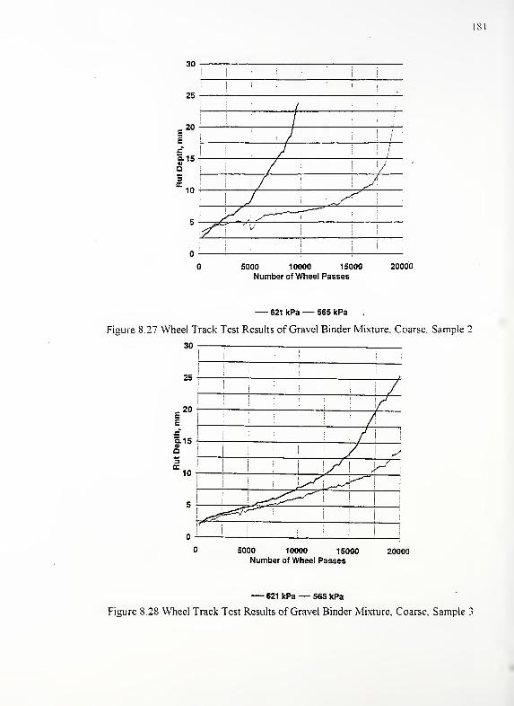
181
30
25
E20
E.e
9.15
10
|
i ! iI !
| j; j
j
/
/
, i
J I /
J I /
; / !/
I / ! ; i J-
i >/ j^-4--—r^-"
I^T "V
!
'
5000 10000 15000 20000
Number of Wheel Passes
— 621 kPa— 565 kPa
Figure 8.27 Wheel Track Test Results of Gravel Binder Mixture, Coarse. Sample 2
30
5000 10000 15000 20000Number of Wheel Passes
— 621 kPa— 565 kPa
Figure 8.28 Wheel Track Test Results of Gravel Binder Mixture, Coarse. Sample 3
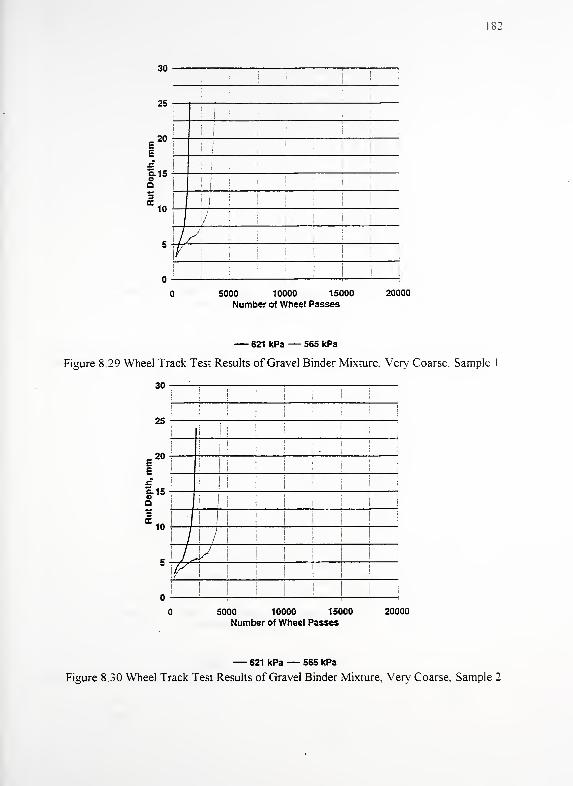
182
30
25
20
Q-15
10
5000 10000 15000 20000
Number of Wheel Passes
— 621 kPa— 565 kPa
Figure 8.29 Wheel Track Test Results of Gravel Binder Mixture, Very Coarse. Sample
30
25
20
9-15
10
5000 10000 15000 20000
Number of Wheel Passes
— 621 kPa— 565 kPa
Figure 8.30 Wheel Track Test Results of Gravel Binder Mixture, Very Coarse, Sample 2
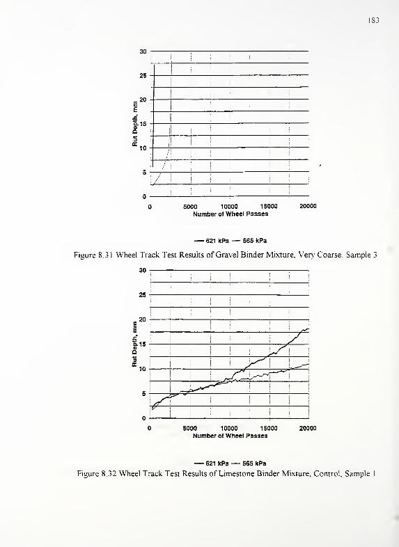
30
25
£20
E
£a.15oQ
110
I I! :
i
j
I
I
|
I
j i
I
I!
;
! /! :
!/ I I i
5000 10000 15000
Number of Wheel Passes20000
— 621 kPa — 565 kPa
Figure 8.3 1 Wheel Track Test Results of Gravel Binder Mixture, Very Coarse. Sample 3
30
25
£20
E
9-15
10
|ll!j :
: i 'i
' '
!
i i
!;
j Jy
\S*\
^^ —
^
i
| ^/f^L^~H—
i
>^<^""
/lI
i II I
ri
i
i
i
i i
i
5000 10000 15000 20000
Number of Wheel Passes
— 621 kPa— 565 kPa
Figure 8.32 Wheel Track Test Results of Limestone Binder Mixture, Control. Sample
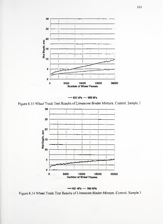
30
25
184
E2°-
tisi-
5000 10000 15000
Number of Wheel Passes
20000
— 621 kPa— 565 kPa
Figure 8.33 Wheel Track Test Results of Limestone Binder Mixture, Control, Sample 2
30
25
20
5000 10000 15000Number of Wheel Passes
20000
— 621 kPa— 565 kPa
Figure 8.34 Wheel Track Test Results of Limestone Binder Mixture, Control. Sample 3
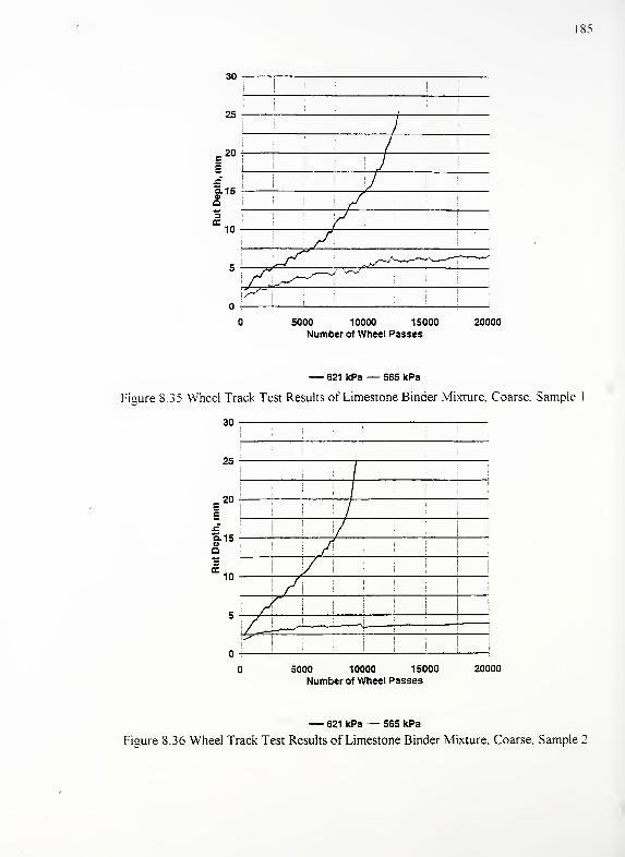
185
ou .
—i
!
!
i !
22 ''
f
r°; i
: \JI
f1- !
!/ '
!
Q I !/J
= 10 ! / '
^-^ ^^A_—"
\ r^:^, j \~y ;
~t^~\i
: !
5000 10000 15000 20000
Number of Wheel Passes
— 621 kPa — 565 kPa
Figure 8.35 Wheel Track Test Results of Limestone Binder Mixture, Coarse. Sample
30
25
20
a. 15
10
r-
5000 10000 15000 20000
Number of Wheel Passes
— 621 kPa — 565 kPa
Figure 8.36 Wheel Track Test Results of Limestone Binder Mixture, Coarse, Sample 2
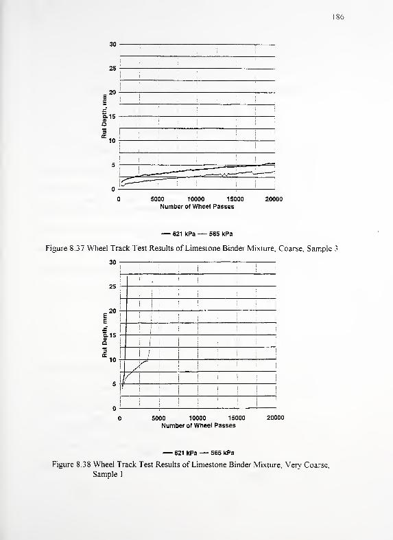
30
25
86
20
V 5
a
10
5000 10000 15000
Number of Wheel Passes20000
— 621 kPa— 565 kPa
Figure 8.37 Wheel Track Test Results of Limestone Binder Mixture, Coarse, Sample 3
30
25
20
9-15
10
j ! jj
i j|
! j Ij j ill
i
ji ! j
:
Ml !
;
li. ._,
1 ! / 1 i
!i jr\
\i \ \
\\r \ \ \ \ \
f | | |;
!
I 1
5000 10000 15000
Number of Wheel Passes
20000
— 621 kPa— 565 kPa
Figure 8.38 Wheel Track Test Results of Limestone Binder Mixture, Very Coarse,
Sample l
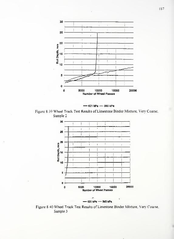
187
30
25
20
8- 15oo
10
^,rL^-"--*-'
:
i:
5000 10000 15000
Number of Wheel Passes20000
— 621 kPa— 565 kPa
Figure 8.39 Wheel Track Test Results of Limestone Binder Mixture, Very Coarse,
Sample 2
30 :
j
;
I i !i
ii
'I I
I
5000 10000 15000
Number of Wheel Passes
20000
— 621 kPa— 565 kPa
Figure 8.40 Wheel Track Test Results of Limestone Binder Mixture. Very Coarse,
Sample 3
88
CHAPTER 9 CONCLUSIONS AND RECOMMENDATIONS
91 Characterization of Segregation
Asphalt mixture segregation is the nonuniform distribution of coarse and fine
aggregate components. With segregation there are physical characteristics that are
measurably different than the non-segregated mixture. This is true for both fine and
coarse segregation. These characteristics include a change in density, asphalt content and
air voids. Fine segregation has a lower percentage of air voids, lower density, and higher
asphalt content than the non-segregated mixture. Coarse segregation has lower asphalt
content and higher percentage of air voids resulting in a dramatically lower density than
9.2 State of Practice
The survey conducted of State Highway Agencies (SHA) supported the need for a
rapid non-destructive testing method for segregation detection. Subjective visual
evaluation in combination with extraction and gradations as used by several SHA's
would seem to be resource intensive.
Of those states that do utilize a nuclear gauge for detection of segregation, the
basis for detection is mainly density differences. Current studies have not shown density
variation to be a reliable indicator of segregation as discussed in section 2.3.

189
The specifications that are used by many agencies concentrate on post-mixim
HMA segregation. Segregation also needs to be addressed during mix design,
stockpiling and plant operations.
9.3 Non-Destructive Detection of Segregation
As discussed in Chapter four, thermal imaging did confirm visual location of
segregated areas. However, the technology was not considered effective in locating
segregation occurring beneath the surface. Also discussed earlier was the insufficiency
of the air permeameter in detecting hidden segregation. This is evident when examining
Figures 5.4 through 5.11.
9.3.2 Nuclear Gauge
Results show that the nuclear moisture/density gauge can be used effectively to
identify variations in asphalt mixture physical properties that can be attributed to
segregation. The results show that the nuclear moisture/density gauge has the potential to
be used in the quality control process to identify in place segregation Results show that
a four minute nuclear gauge reading was found to minimize the measurement error of
density and moisture (asphalt) content. Readings of shorter duration provide somewhat
higher variation.
A bias analysis and subsequent GLM analysis of the correction factors indicated

190
that degree of segregation had no effect on the nuclear density readings Results of the
GLM analysis also indicated that the nuclear gauge density reading varied with differing
base pavement for the limestone mixtures. The combined analysis showed that the
nuclear gauge readings varied with the type of aggregate in the mix The nuclear gauge
overpreidcted the densities of the limestone mixes. The combined analysis also showed
that mixture type (#1 1 Surface or #8 Gravel) had no effect on the nuclear gauge density
readings.
Both the bias analysis and GLM analysis of the correction factors showed that the
nuclear asphalt content readings varied with mixture type, aggregate type, degree of
segregation and base pavement In all cases, the nuclear gauge overpredicted the asphalt
contents of the samples. Results show that the nuclear gauge asphalt content reading
varied with differing as-mixed asphalt contents.
Correction factors may be used to lessen or eliminate the bias caused by the
independent variables of mix type, base pavement and degree of segregation. When
these corrections are made to the data, the nuclear gauge provides results which
accurately predicted density and asphalt content of the samples.
A discriminant analysis showed that the nuclear moisture/density gauge has the
potential to be used effectively to classify a materials degree of segregation. It is
important that the potential exhibited by the results of the study be extended and
evaluated for field conditions.
It is recommended that future studies include an analysis of the effect of varied
asphalt layer thickness on the nuclear gauge density and asphalt content readings. It is
191
also recommended that the studies should include varied segregated layer thickness as a
factor in the design of experiment matrix. -
9.3.3 Permittivity
In permittivity measurement, a limited number of samples were examined, and
thus no conclusions can be made on an experimental basis. However, the tests results
indicate that this technology does exhibit potential to discriminate segregation and should
be studied further.
9.4 Conclusions for Field Tests
9.4 1 Sublot Testing Transverse to Laydown Direction
Sublot testing transverse to laydown direction should be performed utilizing four
minute nuclear gauge measurements. It is apparent that laydown operations can produce
varying levels of segregation transverse to the laydown operation. Because of this
transverse variation in the material, the density test results at transverse locations should
not be averaged as it would be an average for properties of different materials. With
current laydown equipment capability, averaging nuclear gauge measurements should be
done only in the longitudinal direction.

192
9.4.2 Visual Location of Segregation
It has been demonstrated that nuclear gauge testing of visually identified
segregated areas is very effective in quantifying segregation and should be implemented
Based upon field testing with four minute nuclear gauge readings of density and moisture
(asphalt) content, coarse segregation was identified with perfect accuracy The following
implementation of nuclear gauge testing to confirm visual identified segregation is
recommended.
1. A standard background count is taken before use on a daily basis to check
gauge operation and allow for source decay. The new count will pass if
plus or minus two percent of the moisture average and/or plus or minus
one percent of the density average. The operating manual should be
consulted to ensure safe operating procedures.
2. The gauge is operated in backscatter mode. Further, the gauge is operated
in the soil mode allowing for both density and moisture (asphalt) content
measurements.
3. Analysis of coarse segregation is visually identified by an inspector This
area of coarse segregation is defined as an area having considerably more
coarse aggregate than the surrounding acceptable mat and contains little
or no mastic. Figure 9. 1 identifies such an area.
4. A nuclear gauge is placed on the subject location and concurrent four
minute readings of density and moisture (asphalt) content are recorded

5. The density reading is subtracted from the job mix formula target density.
This value is referred to as the "Difference in density from the JMF."
6. The moisture (asphalt) content reading is subtracted from the job mix
formula target asphalt content. This value is referred to as the "Difference
in asphalt content from the JMF."
7. The values obtained in steps 5 and 6 are plotted on Figure 9.2 titled
"Visual Coarse Segregation Classification Based on 4 Minute Nuclear
Gauge Readings."
8. If the plotted point falls below the 90 percent posterior probability line (90
PP), the location is identified as being coarsely segregated.
9.5 Fatigue Characteristics
The flexural fatigue characteristics of segregated hot mix asphalt pavement is
similar to that of non-segregated hot mix. Regression models show that segregated
mixtures are generally parallel to non-segregated mixtures when graphed on a log-log
scale with strain and number of cycles to failure. Finer levels of segregation exhibited
improved fatigue performance, while coarser segregation generally exhibits poorer
performance when compared to non-segregated mixtures at the same strain level This
indicates that from a fatigue standpoint, coarse segregation is critical and could lead to
premature pavement fatigue failure.
Epps and Monismith (1969) concluded that with a fixed asphalt content, the
change in gradation did not affect the fatigue life of mixtures with a 12.5 mm nominal
194
maximum size aggregate. Their work would be indicative of aggregate segregation prior
to combination with asphalt In this case, the segregated aggregate would be combined
with the correct amount of asphalt. The current research would be indicative of
segregation of the optimum mixture after mixing. Thus, segregation occurring in
aggregate stockpiles, cold feed bins, and/or hot bins is not as detrimental to fatigue life as
segregation during mixture storage, transfer, transport and placement
9 6 Permanent Deformation
Permanent deformation testing during laboratory accelerated wheel track testing
indicates that some coarser levels of segregation perform better than the developed
control mixtures (no segregation). Limestone mixtures tested tended to produce more
consistent results than gravel mixtures. This is likely due to the varying mineralogy of
the gravel in samples and/or the variability of the physical characteristics of the gravel
(i.e. crushed faces).
The gross contact pressure during wheel track testing was significant when
stripping occurred, as evident from the gravel binder tests. During the creep phase of a
test and for the overall rate of deformation, the gross contact pressure was also found to
be statistically significant for the limestone surface mixtures but not for any of the other
surface or binder mixtures. Use of the stripping inflection points did not prove to be
useful in evaluating mixtures.

195
9.7 Performance of Segregated Mixtures
Examination of the gravel binder mixture shows the very coarse level of
segregation results in reduced pavement performance of 16.8 percent due to fatigue and
49 and 73.3 percent due to wheel track testing at 565 and 621 kPa contact pressure,
respectively. The coarse level of segregation for the gravel binder mixture shows a
reduction of 49.9 percent in performance due to fatigue, but an increase in performance
of 65.7 and 48.9 percent in wheel track testing at 565 and 621 kPa contact pressure,
respectively
The gravel surface mixture did not experience failure at all levels of segregation
in wheel track testing. However, in fatigue testing the gravel surface mixture did
experience reduced performance of 24.1 and 81.6 percent for the coarse and very coarse
levels of segregation when compared to the control. The limestone surface and binder
mixtures were not fatigue tested, so no conclusions can be drawn for these mixtures with
regard to fatigue. Like the gravel surface mixture, not all levels of segregation for the
limestone surface and binder mixtures experienced wheel track testing failure
9.8 Recommendations for Further Study
Areas that warrant further study include theory and application of permittivity,
accelerated wheel track testing, design of paving laydown equipment, and
implementation of a quality control/quality assurance testing program for segregation
measurement. The gradation limits also warrant closer examination.
196
9.8. 1 Non-Destructive Testing Technology
In the area of non-destructive testing, permittivity technology should be pursued
This technology may be able to provide useful information such as volume measurements
and type of base pavement . The volume measurements could include the volume of air,
asphalt and aggregate. This would enhance detection of segregation. With the recent
development of technology, a vector network analyzer may not be needed to assist in the
measurement of permittivity. As a result, a more cost-effective device could measure
permittivity at predetermined frequencies rather than using a $130,000 vector network
analyzer that measures all frequencies.
9.8.2 Laboratory Accelerated Wheel Track Testing
It has been demonstrated that a laboratory wheel test device can be used to
effectively evaluate compacted bituminous mixtures in a reasonable period of time.
However, sample to sample variation can make it difficult to reach definitive conclusions
with respect to wheel track testing. Realizing this, there are two approaches that could be
pursued.
The first is to improve sample preparation process. However, the variability of
the aggregate may still be significant enough to produce sample to sample variation. The
second improvement is to improve wheel track testing boundary conditions. These
boundary conditions mainly apply to gross contact pressure. Samples could be tested
over a range of gross contact pressures. They could potentially be tested at five different
gross contact pressures from 200 kPa up to 2000 kPa. Similar to the fatigue test, the
197
number of wheel passes to failure verses the contact pressure could be graphically
represented This type of testing would need to be performed on pavements that have a
history of both good and poor performance to establish a standard.
9.8.3 Paving Laydown Equipment
Review of Figures 6.14-6.18 suggests that transverse segregation is a result of
poor operation of the laydown equipment or design flaws in the laydown equipment.
9.8.4 Quality Control/Quality Assurance
In order to initiate an effective quality control/quality assurance (QC/QA)
program, the type of density measured in the mixture design and in the field inspection
must be the same. Without the two types of density being the same, the field
measurement and how to correct it to the design density becomes questionable.
With the introduction of Superpave, the design density is based upon the saturated
surface dry density (Asphalt Institute, 1995). However, it has been demonstrated that this
technique is inadequate in measuring the true density of field samples that are coarsely
segregated. Utilizing the paraffin coating technique may produce more accurate density
measurements. However, the field samples could not be extracted to determine the
asphalt content. Not obtaining the asphalt content from the same samples as the density
would compromise a QC/QA program. This compromise would be especially true if it
includes detecting segregation. The binder ignition test might be applicable to determine
binder content. However, to date there is no experience in using the National Center for

198
Asphalt Technology Furnace method for burning off asphalt and paraffin and thus no
ignition tests were conducted in this study.
9.8.5 Gradation Limits
The INDOT gradation limits should be examined to determine the impact of the
current limits on pavement performance. The coarse level of segregation compared to
the control may perform better as a mixture when both fatigue and wheel track testing are
considered.
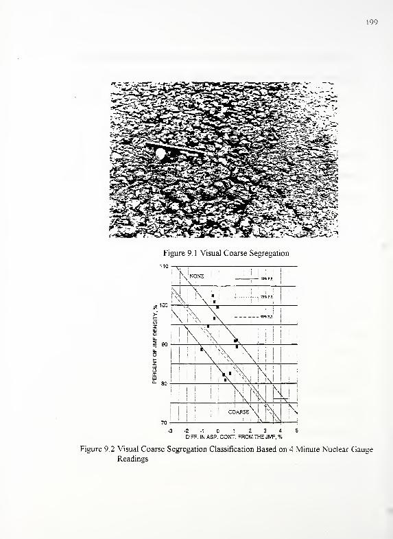
199
Figure 9. 1 Visual Coarse Segregation
110
' N NONE\
M !
x\
100
§ 90\
v>
\i
i
Ii
iN80
70
! : \ I «COARSE \ I
-3-2-10 1 2 3 4 5
DIFF. IN ASP. CONT. FROM THE JMF, %
Figure 9.2 Visual Coarse Segregation Classification Based on 4 Minute Nuclear GaugeReadings

200
LIST OF REFERENCES
201
LIST OF REFERENCES
Al-Qadi, I.L., Ghodgaonkar, D.K., Varadan, V.K., Varadan, V.V., "Effect of Moisture on
Asphaltic Concrete at Microwave Frequencies," IEEE Transactions on Geoscience and
Remote Sensing, Vol. 29, No. 5, pp 710-717, September, 1991.
American Society for Testing and Materials, "Annual Book of ASTM Standards,"
Section 4, Construction, Volume 4.03, ASTM, Philadelphia, PA, 1994
The Asphalt Institute, "Mix Design Methods for Asphalt Concrete and Other Hot Mix
Types," MS-2, Lexington, KY, 1995.
Badaruddin, S., White, T. D., "Asphalt Mix Design and Performance", Joint Highway
Research Project, Purdue University, West Lafayette, IN, FFrWA/IN/JHRP-94/3, May1994.
Badaruddin, S., Kuczek, T., White, T. D., "Identification of Distress Potential in
Bituminous Mixtures Using Discriminant Analysis", Preprint TRB 1994, Washington
DC, January 1994.
Belt, G, Hansen, M., Santelli, N. "Evaluation ofNew Nuclear Density Gauges on
Asphalt Concrete," Scientex Corporation, Rockville, MD, FFTWA, McLean, VA, FFTWA-RD-90-092, September, 1991.
Brock, J.D., "Segregation in Asphalt Mixtures," Proceedings . Association of Asphalt
Paving Technologists, Volume 55, 1986, pp 269-276.
Brown, E.R., and Brownfield, J.R., "Investigation of Rutting and Segregation of Asphalt
Mixtures in the State of Georgia," Georgia Department of Transportation, Atlanta, GA,
FHWA/GA-88/8703.
Brown, E.R., Collins, R., Brownfield, J.R., "Investigation of Asphalt Segregation in State
of Georgia," Paper presented at 68th Annual Meeting of the Transportation Research
Board, Washington, DC, 1989.
Brown, K., Personal communication concerning nuclear gauge testing, 1993.
Brown, K., Personal communication concerning nuclear gauge testing, 1994
Brown, K., Personal communication concerning nuclear gauge testing, 1995
Bryant, L.J , "Effect of Segregation of an Asphaltic Concrete Mixture on Extracted
Asphalt Percentage," Proceedings . Association of Asphalt Paving Technologists, Denver.
CO, Vol. 36, February, 1967, pp 206-218.
Christensen, D.W., Tarris, J. P., "Nuclear Method for Determination of Asphalt Content
Corrected for Moisture in Bituminous Mixtures," Pensylvania Transportation Institute.
Pennsylvania State University, University Park, PA, FHWA/PA-89-008+86- 1 4, May,
1989.
Cody, Ronald P., Smith, JefFery K., "Applied Statistics and the SAS Programming
Language", Prentice-Hall, Inc., Englewood Cliffs, NJ, 1991.
Collins, Personal communication concerning the Georgia Loaded Wheel Tester, 1996
Colorado Department of Transportation, "French Rutter Test Procedure," Colorado
Department of Transportation, Materials Laboratory, Denver, CO, May, 1996.
Cross, S.A., and Brown, E.R., "Effect of Segregation on Performance of Hot Mix
Asphalt," Highway Research Center, Auburn University, AL, Preprint TRB-1993,
Washington, DC, January, 1993.
Epps, J. A. and Monismith, C.L., "Influence of Mixture Variables on the Flexural Fatigue
Properties of Asphalt Concrete," Proceedings , Association of Asphalt Paving
Technologists, Volume 38, 1969, pp 432-458.
Elton, D.J., "Expert Systems for Diagnosing Hot Mix Asphalt Segregation".
Transportation Research Record 1217, Washington, DC, 1989, pp 38-45.
Gupta, Anil, "Temperature and Seasonal Corection Factors for Flexible and Rigid
Pavements," A Thesis Submitted to the Faculty of Purdue University, August, 1987.
Habermann, J.H., "Design Features and a Preliminary Study of the Purdue Linear
Compactor and the PurWheel Tracking Device," A Thesis Submitted to the Faculty of
Purdue University, August, 1994.
Hamburg Road Authority, "Hamburg Road Authority Specifications," City of HamburgConstruction Bureau, Hamburg, Germany, 1992.
Higgins, J. P., LeBlanc, R., Robitaille, R , "Methods of Using Nuclear Gages on
Bituminous Pavement", 25th Annual Convention of the Canadian Technical Asphalt
Association, Victoria, November 1980.
203
Indiana Department of Transportation, "Standard Specifications," INDOT, Indiana
Government Center, Indianapolis, IN, 1993.
James, Mike, "Classification Algorithms," Collins Professional and Technical Books.
London, 1985.
Kallas, B.F., and Puzinauskas, V.P., "Flexural Fatigue Tests on Asphalt Paving
Mixtures," Fatigue of Compacted Bituminous Aggregate Mixtures, American Society for
Testing and Materials, STP 508, Philadelphia, PA, 1972.
Kandhal, P.S. and Klotz, R.C., "Determination of Moisture Contents in Bituminous
Mixtures by Nuclear Method", Transportation Research Record 695, Washington, DC,1978, pp 41-47.
Kennedy, T.W., Tahmoressi, M., Holmgreen, R.J., Jr., Anagnos, J.N., "Segregation of
Asphalt Mixtures - Causes, Identification and Cures," Center for Transportation
Research, Austin, TX, FHWA/TX-87/67+366-1F, November, 1986
Kennedy, T.W., Tahmoressi, M., Solaimanian, M., "Evaluation of a Thin Lift Nuclear
Density Gauge," Transportation Research Record 1217, Washington, DC, 1989,
pp9-19.
Khedaywi, T.S., White, T.D., "Development and Analysis of Laboratory Techniques for
Simulating Segregation," Paper presented at the 74th Annual Meeting of the
Transportation Research Board, Washington, DC, 1994.
Khedaywi, T.S., White, T.D., "Effect of Segregation on Fatigue Performance of Asphalt
Paving Mixtures," Paper presented at the 75th Annual Meeting of the Transportation
Research Board, Washington, DC, 1995.
Labtech Notebook, Laboratory Technologies Corporation, 400 Research Drive,
Wilmington, MA, 1991.
Lackey, W.M., "Segregation - A Mutual Problem", presented at the 31st Annual
Convention of the National Asphalt Pavement Association, Honolulu, HA, 1986.
Lai, James S., "User's Manual: Georgia Loaded Wheel Tester and Rolling Compactor,"
Georgia Institute of Technology, Atlanta, GA, October, 1994.
Missouri Highway and Transportation Department, Materials and Research, "Density of
Thin Lift Bituminous Mixtures By Nuclear Methods," Missouri Highway and
Transportation Department, Division of Materials and Research, Jefferson City, MO.MCHRP 90-1, May, 1991.
204
Nady, R.M., "Resurfacing: Construction Problems. Solutions "", Proceedings .
Association of Asphalt Paving Technologists, Vol. 53. 1984.
Parti, M.N., Vinson, T.S., Hicks, R.G., Younger, K.D., "Experimental Study on
Mechanical Properties of Stone Mastic Asphalt," Transportation Research Institute.
Oregon State University, Corvallis, OR, March, 1995.
Regan, George L., "Evaluation of a Nuclear Asphalt Content Gauge," U.S. Army
Engineer Waterways and Experiments Station, Vickburg, MI, S-75-23, October, 1975.
Roberts, Freddy L., Kandhal, Priviti S., Brown, E.R., Lee, Dah-Yinn, Kennedy, Thomas
W , "Hot Mix Asphalt Materials, Mixture Design and Construction,'* N.APA Education
Foundation, National Center for Asphalt Technology, Lanham, MD, 1991
SAS Institute Inc., "SAS System for Regression," Cary, NC, 1991
Shahin, MY. and Kohn, S.D., "Development of Pavement Condition Rating Procedures
for Roads, Streets, and Parking Lots - Volume I Condition Rating Procedure." Technical
Report M-268, Construction Engineering Research Laboratory, United States Corps of
Engineers, 1979.
Troxler Electronic Laboratories, Inc., "User Instruction Manual for the 3440 Nuclear
Density Gauge," Research Triangle Park, NC, 1988.
Troxler Electronic Laboratories, Inc., "Review of the 3400 Series Soils GaugeOperation," Research Triangle Park, NC, 1993.
White, Thomas D., "Porous Friction Surface Course," U.S. Army Engineer Waterways
and Experiments Station, Vickburg, MI, FAA-RD-73-197, February, 1975.
Williams, R.C., Duncan, G.D., White, T.D., "Sources and Measurement of Segregated
Hot Mix Asphalt Pavement," Paper presented at the 76th Annual Meeting of the
Transportation Research Board, Washington, DC, 1996.
Yoder, E.J. and Witzak, M.W., "Principles of Pavement Design," John Wiley & Sons.
Inc., New York, 1975.
Zube, E., "Compaction Studies of Asphalt Concrete Pavement as Related to the Water
Permeability Test," Paper presented at 41st Annual Meeting of the Highway Research
Board, Washington, DC, 1962.

205
APPENDICES
206
APPENDIX AState of Practice Survey Results
207
1284 Civil Engineering
Civil Engineering Building Rm. B150Bituminous Materials Laboratory
Purdue University
West Lafayette, IN 47907-1284
To Whom it May Concern:
I am currently involved in an ongoing research project under Dr. Thomas D. White for the
Indiana Department of Transportation (INDOT) Research Division concerning segregation in hot
mix asphalt (HMA). I am conducting a survey to determine techniques for prevention of
segregation in HMA for the various state agencies across the country. The results of this study
will be included in my masters thesis. My thesis involves quantifying segregation and
determining a rapid, non-destructive field test to determine the presence of segregation. I am also
compiling and producing a video that addresses solutions to common problems in construction
and placement of HMA that cause segregation.
Filling out this short questionnaire will be helpful to me and my research. Please take ten
minutes to fill this out and return it in the enclosed, stamped envelope. If I have sent this to the
wrong person, please forward it to the individual in your agency who could address the matters
presented in the survey.
Thank you for your time.
Sincerely,
Gary R. Duncan Jr.
Research Assistant
Purdue University

208
Questionnaire Concerning DOT Guidelines/Procedures in Prevention of Segregation in
HMA.Gary R Duncan Jr. Research Assistant
Purdue University
16 FEB 94
1. Does your agency have any specifications or guidelines for the prevention of
segregation in Hot Mix Asphalt (HMA) during the phases of production and
placement?
2. Does your agency train technicians in any trouble-shooting procedures to
rmnimize segregation in the production and placement of quality HMA?
3. Does your agency make any attempts to quantify the degree of segregation
(i.e. testing, visual evaluation) when it is known to exist?
4. Does your agency have a reduction in pay factor for stripping? If so, what
is the basis for deciding the reduction?
5. Would your agency be interested in training material or presentations
concerning procedures to rniriimize segregation in HMA production
and placement?
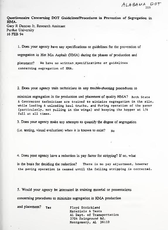
ALA-GAM* OCT209
Questionnaire Concerning DOT Guidelines/Procedures in Prevention of Segregation in
HMA.Gary R Duncan Jr, Research Assistant
Purdue University
16 FEB 94
1. Does your agency have any specifications or guidelines for the prevention of
segregation in Hot Mix Asphalt (HMA) during the phases of production and
placement? We have no written specifications or guidelines
concerning segregation of HMA.
2. Does your agency train technicians in any trouble-shooting procedures to
minimize segregation in the production and placement of quality HMA? Both State
& Contractor technicians are trained to minimize segregation in the silo,
while loading & unloading haul trucks, and during operation of the paver
(particularly, not pulling in the wings) and keeping the hopper at 1/4
full at all times.
3. Does your agency make any attempts to quantify the degree of segregation
(i.e. testing, visual evaluation) when it is known to exist? No
4. Does your agency have a reduction in pay factor for stripping? If so, what
is the basis for deciding the reduction? There is no pay adjustment, however
the paving operation is ceased until the failing stripping is corrected,
5. Would your agency be interested in training material or presentations
concerning procedures to minimize segregation in HMA production
and placement? yes Floyd StricklandMaterials & TestsAL Dept. of Transportation3704 Fairground Rd.
Montgomery, AL 36110
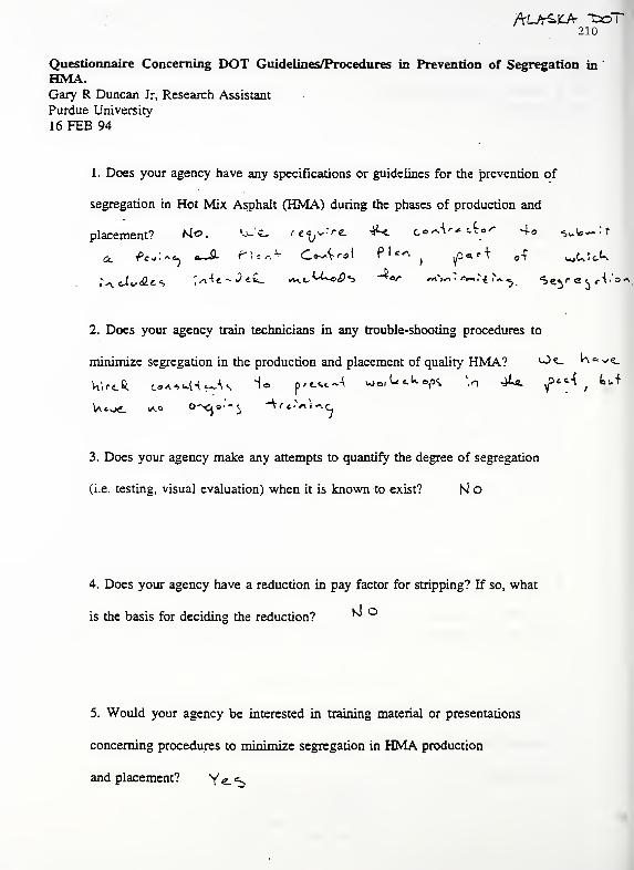
210
Questionnaire Concerning DOT Guidelines/Procedures in Prevention of Segregation in
HMA.Gary R Duncan Jr. Research Assistant
Purdue University
16 FEB 94
1. Does your agency have any specifications or guidelines for the prevention of
segregation in Hot Mix Asphalt (HMA) during the phases of production and
placement? no . ijJc r e$.^ ;/"e. 4^t c«
o_ Pc^"*-. a. .}*- r">^> Co^^rai)
,\J«/£tS >4f.Ja£_ ^0*^-0^*5 4- 0«N
2. Does your agency train technicians in any trouble-shooting procedures to
minimize segregation in the production and placement of quality HMA? ^^- ^ & yJ 'z-
oWrtft WA^H^s io prt^c-4 wo. <<«>«/*V
,^l 4U ^>«Mi
feu +
3. Does your agency make any attempts to quantify the degree of segregation
(i.e. testing, visual evaluation) when it is known to exist? Si O
4. Does your agency have a reduction in pay factor for stripping? If so, what
is the basis for deciding the reduction? ™ °
5. Would your agency be interested in training material or presentations
concerning procedures to minimize segregation in HMA production
and placement? Ye^
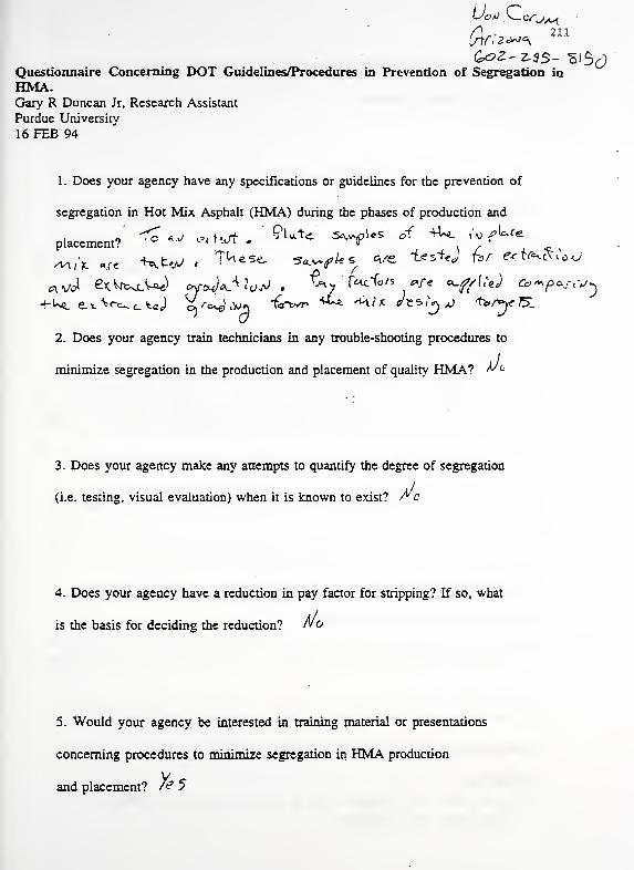
Questionnaire Concerning DOT Guidelines/Procedures in Prevention of Segregation in
HMA.Gary R Duncan Jr. Research Assistant
Purdue University
16 FEB 94
1. Does your agency have any specifications or guidelines for the prevention of
segregation in Hot Mix Asphalt (HMA) during the phases of production and
placement?
2. Does your agency train technicians in any trouble-shooting procedures to
minimize segregation in the production and placement of quality HMA? ^c
3. Does your agency make any attempts to quantify the degree of segregation
(i.e. testing, visual evaluation) when it is known to exist? Ac
4. Does your agency have a reduction in pay factor for stripping? If so, what
is the basis for deciding the reduction? N
o
5. Would your agency be interested in training material or presentations
concerning procedures to minimize segregation in HMA production
and placement? 7& 5
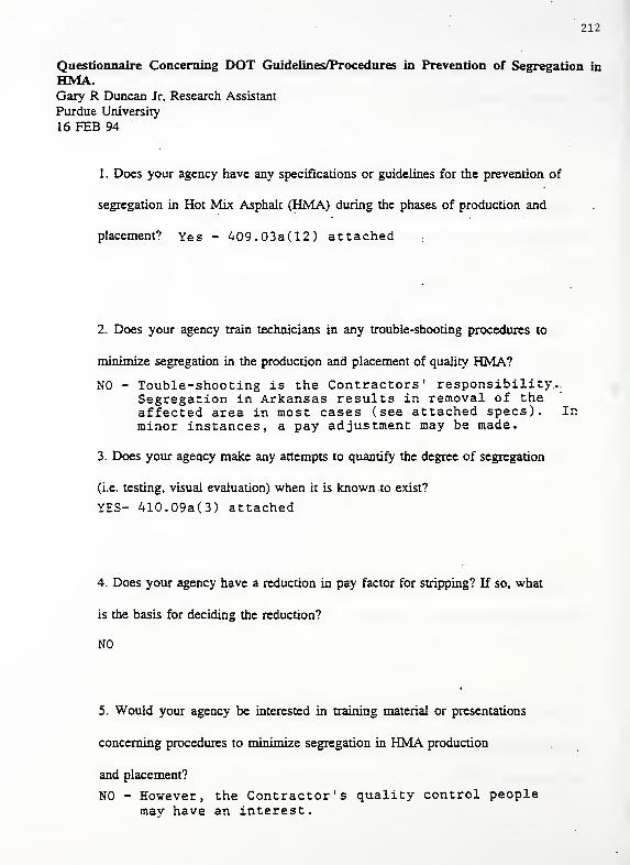
212
Questionnaire Concerning DOT Guidelines/Procedures in Prevention of Segregation in
HMA.Gary R Duncan Jr, Research Assistant
Purdue University
16 FEB 94
1. Does your agency have any specifications or guidelines for the prevention of
segregation in Hot Mix Asphalt (HMA) during the phases of production and
placement? Yes - 409.03a(12) attached
2. Does your agency train technicians in any trouble-shooting procedures to
minimize segregation in the production and placement of quality HMA?
NO - Touble-shooting is the Contractors' responsibility...Segregation in Arkansas results in removal of theaffected area in most cases (see attached specs). Inminor instances, a pay adjustment may be made.
3. Does your agency make any attempts to quantify the degree of segregation
(i.e. testing, visual evaluation) when it is known to exist?
YES- 410.09a(3) attached
4. Does your agency have a reduction in pay factor for stripping? If so, what
is the basis for deciding the reduction?
NO
5. Would your agency be interested in training material or presentations
concerning procedures to minimize segregation in HMA production
and placement?
NO - However, the Contractor's quality control peoplemay have an interest.
CCICRADO213
Questionnaire Concerning DOT Guidelines/Procedures in Prevention of Segregation in
HMA.Gary R Duncan Jr, Research Assistant
Purdue University
16 FEB 94
1. Does your agency have any specifications or^guidelines) for the prevention of
segregation in Hot Mix Asphalt (HMA) during the phases of production and
placement?Colorado DOT requires the contractor to document steps he will take to prevent
and correct segregation if it occurs during the prepaving conference.
2. Does your agency train technicians in any trouble-shooting procedures to
minimize segregation in the production and placement of quality HMA?CDOT has sponsored training for both CDOT and Contractor personnel at no costfor the. last three years (4 sessions of 2 days each) following the "Hot Mix PavingHandbook" ( AASHTO, FHWA, etc.) and the increased awareness on the part of bothparties has greatly reduced segregation problems on our projects.
We hired J. Scherocman to present training)3. Does your agency make any attempts to quantify the degree of segregation
(i.e. testing, visual evaluation) when it is known to exist?
(See attached DRAFT test method)
This method was seldom tried and never used as a specification. Segregationhas to be pretty bad visually before this procedure shows much.
4. Does your agency have a reduction in pay factor for stripping? If so, what
is the basis for deciding the reduction?
When project produced hot mix fails the Lottman test, the contractor is required to
stop production and correct mix problems prior to restart of paving.
5. Would your agency be interested in training material or presentations
concerning procedures to minimize segregation in HMA production
and placement?
Yes
214
Questionnaire Concerning DOT Guidelines/Procedures in Prevention of Segregation in
(HMA)Gary R Duncan Jr, Research Assistant
Purdue University
16 FEB 94
1. Does your agency have any specifications or guidelines for the prevention of
segregation in Hot Mix Asphalt (HMA) during the phases of production and
placement?
See copy of specifications attached. Areas that pertain
to segregation are high-lighted in red.
2. Does your agency train technicians in any trouble-shooting procedures to
minimize segregation in the production and placement of quality HMA?
YES
3. Does your agency make any attempts to quantify the degree of segregation
(i.e. testing, visual evaluation) when it is known to exist?
Visual evaluation followed by selective sampling and
testing; e.g. , right and left or front and back of truck
to search for variations in grading.
4. Does your agency have a reduction in pay factor for stripping? If so, what is
the basis for deciding the reduction?
NO
5. Would your agency be interested in training material or presentations
concerning procedures to minimize segregation in HMA production
and placement?
YES
C d>'£- l>'M £>>A 215
Questionnaire Concerning DOT Guidelines/Procedures in Prevention of Segregation inHMA.Gary R Duncan Jr, Research Assistant
Purdue University
16 FEB 94
1. Does your agency have any specifications or guidelines for the prevention of
segregation in Hot Mix Asphalt (HMA) during the phases of production and
placement?YES - SPECIFICATIONS
A. AASHTO M-I55B. STANDARD OPERATING PROCEDURESC. DC STANDARD SPECIFICATIONS 801.05D. DC STANDARD SPECIFICATIONS 401.07E. INSPECTORS ARE ASSIGNED TO HMA PLANTS AND PAVING SITES
2. Does your agency train technicians in any trouble-shooting procedures to
minimize segregation in the production and placement of quality HMA?
YES
3. Does your agency make any attempts to quantify the degree of segregation
(i.e. testing, visual evaluation) when it is known to exist?
NO
4. Does your agency have a reduction in pay factor for stripping? If so, what
is the basis for deciding the reduction?
NO
5. Would your agency be interested in training material or presentations
concerning procedures to rninimize segregation in HMA production
#SdA>feg
e5f^YS RECEPTIVE TO IMPROVEMENTS IN OUR INSPECTION ANDTESTING PROCEDURES
FLORIDA216
Questionnaire Concerning DOT Guidelines/Procedures in Prevention of Segregation in
HMA.Gary R Duncan Jr. Research Assistant
Purdue University
16 FEB 94
1. Does your agency have any specifications or guidelines for the prevention of
segregation in Hot Mix Asphalt (HMA) during the phases of production and
(Florida Department of Transportation)placement? (FDOT) Specifications prohibit segregation in Hot Mix
Asphalt (HMA) but do not include guidelines or methods for preventionduring production and placement.
2. Does your agency train technicians in any trouble-shooting procedures to
minimize segregation in the production and placement of quality HMA?Yes, all of the techniques that are known to prevent segregation, fromhandling of the stockpiles to the paving operations:, are taught as partof the Asphalt Plant and Paving Technician Certification courses.'
3. Does your agency make any attempts to quantify the degree of segregation
(i.e. testing, visual evaluation) when it is known to exist?
Yes, a visual evaluation is made of the texture of each pavement layer.The Contractor is then required to correct any areas having unacceptabletexture due to segregation (See attached Specification, Subarticle 330-12.2.)
4. Does your agency have a reduction in pay factor for stripping? If so, what
is the basis for deciding the reduction?
No. Stripping has not been a problem in Florida; however, if an excessiveamount of stripping were to be detected in a pavement prior to finalacceptance it would be removed and replaced.
5. Would your agency be interested in training material or presentations
concerning procedures to minimize segregation in HMA production
and placement?
Yes, any new material would be appreciated.
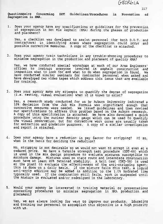
Cr&XbiAin
Questionnaire Concerning DOT Guidelines/Procedures in Prevention ofSegregation in HMA.
1. Does your agency have any specifications or guidelines for the preventionof segregation in Hot Mix Asphalt (HMA) during the phases of productionand placement?
Yes, a checklist was developed to assist personnel (for both D.O.T. andcontractors) in identifying areas where segregation could occur andpossible corrective measures. A copy of the checklist is attached.
2. Does your agency train technicians in any trouble-shooting procedures tominimize segregation in the production and placement of quality HMA?
Yes, we have conducted special workshops at each of our Area Engineers'offices to instruct everyone involved in asphalt construction andinspection what to look for and what to do when segregation is found. Wehave conducted similar seminars for contractor personnel when asked andhave developed two video tapes which address this issue that are availablefor training.
3
.
Does your agency make any attempts to quantify the degree of segregation(i.e. testing, visual evaluation) when it is known to exist?
Yes, a research study conducted for us by Auburn University indicated a10% deviation from the Job Mix Formula was significant enough thatcorrective measures were needed. We issued guidelines and then revisedour specifications to address this problem based on the Auburn research.A copy of this specification is attached. We have also developed a quickprocedure using the nuclear density gauge which can be used to quantifythe visual observation, but for corrective work cores are usually takenfor extraction and gradation purposes. A copy of a similar investigationand report is attached.
4. Does your agency have a reduction in pay factor for stripping? If so,what is the basis for deciding the reduction?
No, stripping is not desirable so we would not want to accept it even at areduced price. We have a tensile strength test procedure (GDT-66) whichis used in the mix design procedure to evaluate mixtures susceptible tomoisture damage. Mixtures used on state route and interstate constructionmust have at least 80% retained stability. A boil test (GHD-56) is usedat the plant to evaluate the effectiveness of the anti-stripping agent;this is done on a daily basis. If the mixture fails this test, a liquidanti-strip additive may be added in addition to the 1.0% hydrated limetypically used. If the combination still fails, work is suspended untilthe mixture is evaluated and/or redesigned in the laboratory.
5. Would your agency be interested in training material or presentationsconcerning procedures to minimize segregation in HMA production andplacement?
Yes, we are always looking for ways to improve our products. Educatingand training our personnel to accomplish this objective is a high prioritywith us.
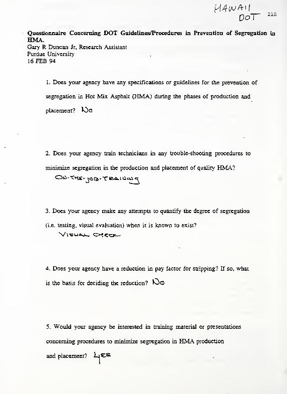
OoT 21G
Questionnaire Concerning DOT Guidelines/Procedures in Prevention of Segregation in
HMA.Gary R Duncan Jr, Research Assistant
Purdue University
16 FEB 94
1. Does your agency have any specifications or guidelines for the prevention of
segregation in Hot Mix Asphalt (HMA) during the phases of production and
placement? 10o
2. Does your agency train technicians in any trouble-shooting procedures to
minimize segregation in the production and placement of quality HMA?OO - "CHE -
J3 Cfc -TE^ t Vi Ui er
3. Does your agency make any attempts to quantify the degree of segregation
(i.e. testing, visual evaluation) when it is known to exist?
4. Does your agency have a reduction in pay factor for stripping? If so, what
is the basis for deciding the reduction? KjO
5. Would your agency be interested in training material or presentations
concerning procedures to minimize segregation in HMA production
and placement? 1jCs
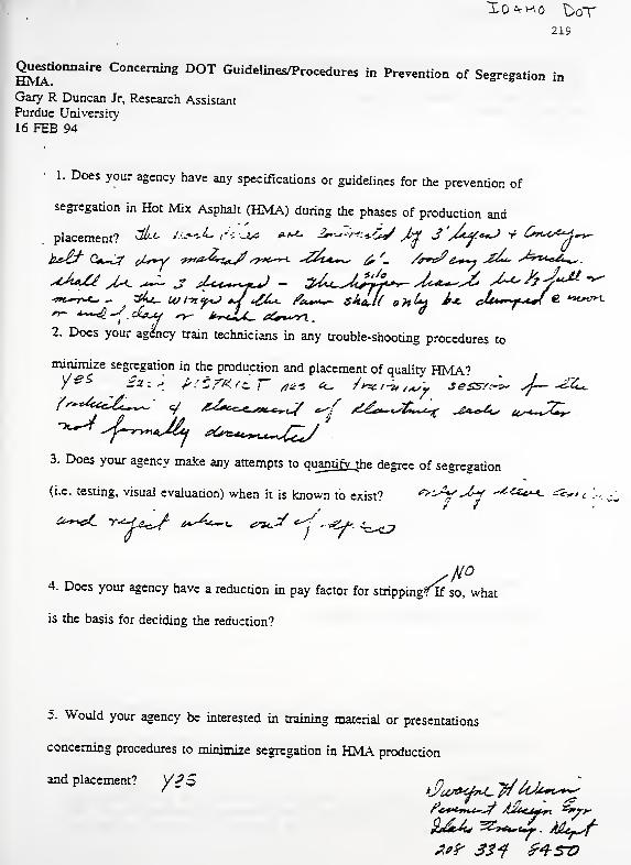
Tcxvho t>oT219
Questionnaire Concerning DOT Guidelines/Procedures in Prevention of Segregation in
Gary R Duncan Jr, Research Assistant
Purdue University
16 FEB 94
1. Does your agency have any specifications or guidelines for the prevention of
segregation in Hot Mix Asphalt (HMA) during the phases of production and
placement? ^ ***£- ''- '-^ **"'- ^»*^«*i/ Jtf 3 '/&t<f**J * CmM**.
*>t~r*~ - Z&L. u/ot^f *J *£/^ f*^~ skartt only J>+ dt**-f-*J € *»t*en.
2. Does your agency train technicians in any trouble-shooting procedures to
minimize segregation in the production and placement of quality HMA?
3. Does your agency make any attempts to quantify the degree of segregation
(i.e. testing, visual evaluation) when it is known to exist7 ^-^V'-^V ****
9 /
4. Does your agency have a reduction in pay factor for stripping^ so, what
is the basis for deciding the reduction?
-*W c
5. Would your agency be interested in training material or presentations
concerning procedures to minimize segregation in HMA production
and placement? y£S J^y^At? 334 &4SO
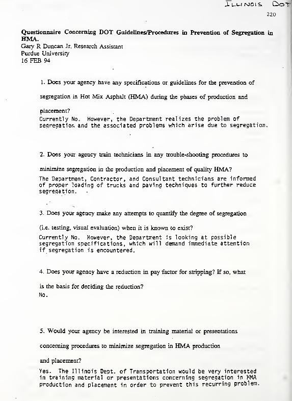
J. ut-i roots. Dot220
Questionnaire Concerning DOT Guidelines/Procedures in Prevention of Segregation in
HMA.Gary R Duncan Jr, Research Assistant
Purdue University
16 FEB 94
1. Does your agency have any specifications or guidelines for the prevention of
segregation in Hot Mix Asphalt (HMA) during the phases of production and
placement?
Currently No. However, the Department realizes the problem ofsegregation and the associated problems which arise due to segregation.
2. Does your agency train technicians in any trouble-shooting procedures to
minimize segregation in the production and placement of quality HMA?The Department, Contractor, and Consultant technicians are informedof proper loading of trucks and paving techniques to further reducesegregation.
3. Does your agency make any attempts to quantify the degree of segregation
(i.e. testing, visual evaluation) when it is known to exist?
Currently No. However, the Department is looking at possiblesegregation specifications, which will demand immediate attentionif segregation is encountered.
4. Does your agency have a reduction in pay factor for stripping? If so, what
is the basis for deciding the reduction?
No.
5. Would your agency be interested in training material or presentations
concerning procedures to minimize segregation in HMA production
and placement?
Yes. The Illinois Dept. of Transportation would be very interestedin training material or presentations concerning segregation in HMA
production and placement in order to prevent this recurring problem.
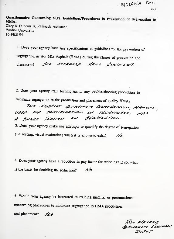
/AjDfA^A DO"
221
Questionnaire Concerning DOT Guidelines/Procedures in Prevention of Segregation inHMA.Gary R Duncan Jr. Research AssistantPurdue University
16 FEB 94
1. Does your agency have any specifications or guidelines for the prevention of
segregation in Hot Mix Asphalt (HMA) during the phases of production and
placement? ^^ SrrSA»/<0 J%7s*>> ^V^^t^^t:
2. Does your agency train technicians in any trouble-shooting procedures to
minimize segregation in the production and placement of quality HMA?
3. Does your agency make any attempts to quantify the degree of segregation
(i.e. testing, visual evaluation) when it is known to exist? A&
4. Does your agency have a reduction in pay factor for stripping? If so, what
is the basis for deciding the reduction? A^d
5. Would your agency be interested in training material or presentations
concerning procedures to minimize segregation in HMA production
and placement? /g$

j-&w a t>crr222
Questionnaire Concerning DOT Guidelines/Procedures in Prevention of Segregation inHMA.Gary R Duncan Jr. Research Assistant
Purdue University
16 FEB 94
1. Does your agency have any specifications or guidelines for the prevention of
segregation in Hot Mix Asphalt (HMA) during the phases of production and
placement? t\j o
2. Does your agency train technicians in any trouble-shooting procedures to
minimize segregation in the production and placement of quality HMA?
3. Does your agency make any attempts to quantify the degree of segregation
(i.e. testing, visual evaluation) when it is known to exist?
4. Does your agency have a reduction in pay factor for stripping? if so, what
is the basis for deciding the reduction? AG O
5. Would your agency be interested in training material or presentations
concerning procedures to minimize segregation in HMA production
and placement? y £5
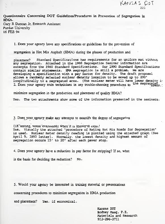
\<AMM s Co'223
Questionnaire Concerning DOT Guidelines/Procedures in Prevention of Segregation in
HMA.Gary R Duncan Jr, Research Assistant
Purdue University
16 FEB 94
1. Does your agency have any specifications or guidelines for the prevention of
segregation in Hot Mix Asphalt (HMA) during the phases of production and
placement? Standard Specifications has requirements for an uniform mat withoutany segregation. Attached in the 1986 Segregation Seminar information areexcerpts from the 1980 Standard Specifications- Our 1990 Standard Specificationscontain similar statements. HMA segregation is still a problem. We aredeveloping a specification with a pay factor for density. The draft proposalallows a randomly selected nuclear density location to be moved up to 200'
longitudinally to a segregated area. (The nuclear meter will have lower density ir
2. Does your agency train technicians in any trouble-shooting procedures tothe segreg
lrlas .
;
minimize segregation in the production and placement of quality HMA?
Yes. The two attachments show seine of the information presented in the seminars.
3. Does your agency make any attempts to auantifv the degree of segregation
Cue.'' testing, visuai'evaiuauoh) wtien'it is khown'to exist/
Yes. Visually the attached "procedure of Rating Hot Mix Roads for Segregation"is used. Nuclear meter density reading is plotted using the attached graph (See
April 9/ 1993 letter). Normally/ the lowest density and highest amount ofsegregation occurs 15' to 20' after each paver stop.
4. Does your agency have a reduction in pay factor for stripping? If so, what
is the basis for deciding the reduction? No.
5. Would your agency be interested in training material or presentations
concerning procedures to minimize segregation in HMA production
and placement? Yes , if economical
.
Kansas DOTRodney Maag/ P.E.Materials and Research913-296-3711
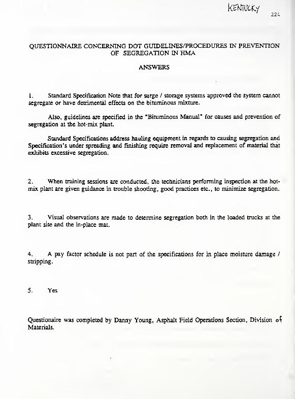
224
QUESTIONNAIRE CONCERNING DOT GUIDELINES/PROCEDURES IN PREVENTIONOF SEGREGATION IN HMA
ANSWERS
1. Standard Specification Note that for surge / storage systems approved the system cannot
segregate or have detrimental effects on the bituminous mixture.
Also, guidelines are specified in the "Bituminous Manual" for causes and prevention of
segregation at the hot-mix plant.
Standard Specifications address hauling equipment in regards to causing segregation and
Specification's under spreading and finishing require removal and replacement of material that
exhibits excessive segregation.
2. When training sessions are conducted, the technicians performing inspection at the hot-
mix plant are given guidance in trouble shooting, good practices etc., to minimize segregation.
3. Visual observations are made to determine segregation both in the loaded trucks at the
plant site and the in-place mat.
4. A pay factor schedule is not part of the specifications for in place moisture damage /
stripping.
5. Yes
Questionaire was completed by Danny Young, Asphalt Field Operations Section, Division o$
Materials.
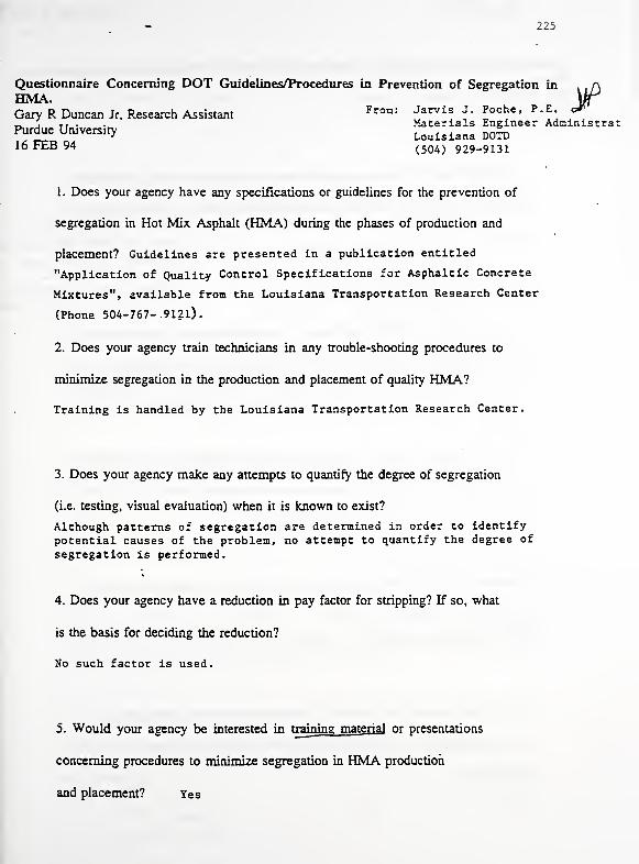
225
Questionnaire Concerning DOT Guidelines/Procedures in Prevention of Segregation in .aHMA. )jrGary R Duncan Jr. Research Assistant
From: Jarvis J. Poche, P.E c*
_, j TT . Materials Engineer AdminiscratPurdue University
Louisiana DOTD16 FEB 94 (504) 929-9131
1. Does your agency have any specifications or guidelines for the prevention of
segregation in Hot Mix Asphalt (HMA) during the phases of production and
placement? Guidelines are presented in a publication entitled
"Application of Quality Control Specifications for Asphaltic Concrete
Mixtures", available from the Louisiana Transportation Research Center
(Phone 504-767-9121).
2. Does your agency train technicians in any trouble-shooting procedures to
minimize segregation in the production and placement of quality HMA?
Training is handled by the Louisiana Transportation Research Center.
3. Does your agency make any attempts to quantify the degree of segregation
(i.e. testing, visual evaluation) when it is known to exist?
Although patterns of segregation are determined in order to identify
potential causes of the problem, no attempt to quantify the degree of
segregation is performed.
4. Does your agency have a reduction in pay factor for stripping? If so, what
is the basis for deciding the reduction?
No such factor is used.
5. Would your agency be interested in training material or presentations
concerning procedures to minimize segregation in HMA production
and placement? Yes
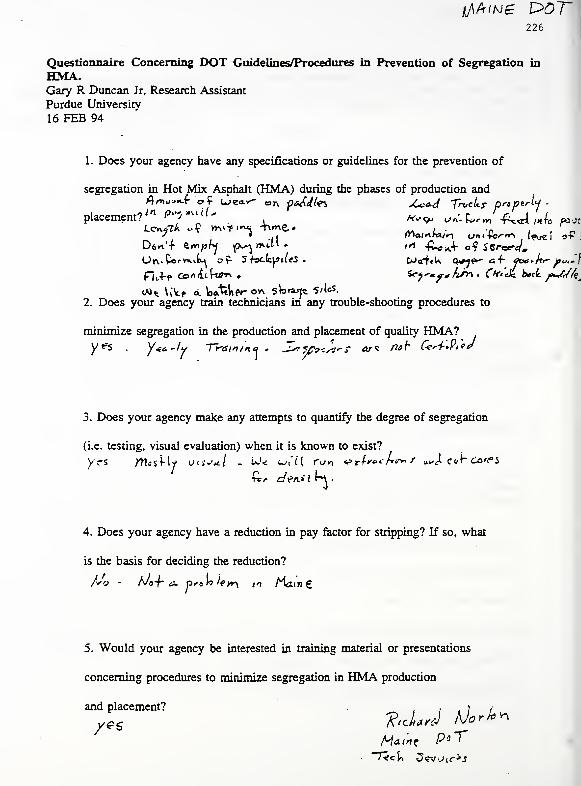
Jt
fJ[AlN£ V>Of226
Questionnaire Concerning DOT Guidelines/Procedures in Prevention of Segregation in
HMA.Gary R Duncan Jr. Research Assistant
Purdue University
16 FEB 94
1. Does your agency have any specifications or guidelines for the prevention of
segregation in Hot Mix Asphalt (HMA) during the phases of production andfimo+*Sr e>? u><e*v- «A paJJl&i /*ca-d. Trucks properly
placement?"1 P"5^«'' *,^ utC. ^m '^^ £ ,
06*' f e*r,/j^ jp^mtLU ,« •ft^A'f o? JCrer*/,
2. Does your agency train technicians in any trouble-shooting procedures to
minimize segregation in the production and placement of quality HMA?y«*s y*<i.~ty Trati/n* » S^ttcs-j-r or* not &**h>9i*J
3. Does your agency make any attempts to quantify the degree of segregation
(i.e. testing, visual evaluation) when it is known to exist?
for den.il rH .
4. Does your agency have a reduction in pay factor for stripping? If so, what
is the basis for deciding the reduction?
5. Would your agency be interested in training material or presentations
concerning procedures to minimize segregation in HMA production
and placement?
MMain? P*T
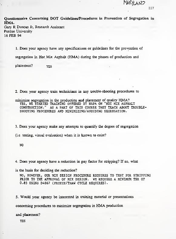
227
Questionnaire Concerning DOT Guidelines/Procedures in Prevention of Segregation in
HMA.Gary R Duncan Jr, Research Assistant
Purdue University
16 FEB 94
1. Does your agency have any specifications or guidelines for the prevention of
segregation in Hot Mix Asphalt (HMA) during the phases of production and
placement? YES
2. Does your agency train technicians in any trouble-shooting procedures to
minirnize segregation in the production and placement of quality HMA?YES, WE STARTED TRAINING OFFERED BY NAPA ON "HOT MIX ASPHALTCONSTRUCTION." AS A PART OF THIS COURSE THEY TEACH ABOUT TROUBLE-SHOOTING PROCEDURES AND MINIMIZING/AVOIDING SEGREGATION.
3. Does your agency make any attempts to quantify the degree of segregation
(i.e. testing, visual evaluation) when it is known to exist?
NO
4. Does your agency have a reduction in pay factor for stripping? If so, what
is the basis for deciding the reduction?
NO, HOWEVER, OUR MIX DESIGN PROCEDURE REQUIRES TO TEST FOR STRIPPINGPRIOR TO THE APPROVAL OF MIX DESIGN. WE REQUIRE A MINIMUM TSR OF0.85 USING D4867 (FREEZE/THAW CYCLE REQUIRED).
5. Would your agency be interested in training material or presentations
concerning procedures to rmmrnize segregation in HMA production
and placement?
YES
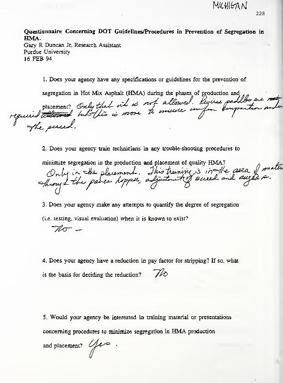
228
Questionnaire Concerning DOT Guidelines/Procedures in Prevention of Segregation in
HMA.Gary R Duncan Jr, Research Assistant
Purdue University
16 FEB 94
1. Does your agency have any specifications or guidelines for the prevention of
segregation in Hot Mix Asphalt (HMA) during the phases of production and
2. Does your agency train technicians in any trouble-shooting procedures to
minimize segregation in the production and placement of quality HMA? ~ /__
3. Does your agency make any attempts to quantify the degree of segregation
(i.e. testing, visual evaluation) when it is known to exist?
4. Does your agency have a reduction in pay factor for stripping? If so, what
is the basis for deciding the reduction? /rt>
5. Would your agency be interested in training material or presentations
concerning procedures to minimize segregation in HMA production
and placement? CA^^3-
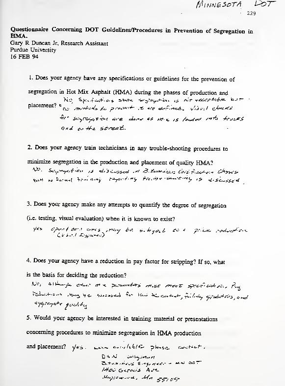
229
Questionnaire Concerning DOT Guidelines/Procedures in Prevention of Segregation inHMA.Gary R Duncan Jr, Research Assistant
Purdue University
16 FEB 94
1. Does your agency have any specifications or guidelines for the prevention of
segregation in Hot Mix Asphalt (HMA) during the phases of production and
'Dc- .tfr'^'^'S* jfc* Z> /WW *+~ .-£. *,*e e&>r '"<£&„ ^iJittt c£***f£
2. Does your agency train technicians in any trouble-shooting procedures to
minimize segregation in the production and placement of quality HMA?
3. Does your agency make any attempts to quantify the degree of segregation
(i.e. testing, visual evaluation) when it is known to exist?
<lii.-/%^,) ' 7 r
4. Does your agency have a reduction in pay factor for stripping? If so, what
is the basis for deciding the reduction?
5. Would your agency be interested in training material or presentations
concerning procedures to minimize segregation in HMA production
and placement? y*?s . ua»-«- +»<ul\kl€~ pi«*.,$«». &**.**<**'*
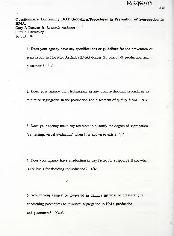
230
Questionnaire Concerning DOT Guidelines/Procedures in Prevention of Segregation in
HMA.Gary R Duncan Jr, Research Assistant
Purdue University
16 FEB 94
1. Does your agency have any specifications or guidelines for the prevention of
segregation in Hot Mix Asphalt (HMA) during the phases of production and
placement? t*)o
2. Does your agency train technicians in any trouble-shooting procedures to
minimize segregation in the production and placement of quality HMA? do
3. Does your agency make any attempts to quantify the degree of segregation
(i.e. testing, visual evaluation) when it is known to exist? Mo
4. Does your agency have a reduction in pay factor for stripping? If so, what
is the basis for deciding the reduction? NO
5. Would your agency be interested in training material or presentations
concerning procedures to nunimize segregation in HMA production
and placement? Y&S

Missouri Pol Z31
Questionnaire Concerning DOT Guidelines/Procedures in Prevention of Segregation in
HMA.Gary R Duncan Jr. Research Assistant
Purdue University
16 FEB 94
1. Does your agency have any specifications or guidelines for the prevention of
segregation in Hot Mix Asphalt (HMA) during the phases of production and
placement?
See attached specification excerpts.
2. Does your agency train technicians in any trouble-shooting procedures to
minimize segregation in the production and placement of quality HMA?
See attached Appendix E.
3. Does your agency make any attempts to quantify the degree of segregation
(i.e. testing, visual evaluation) when it is known to exist?
See attached Appendix E.
4. Does your agency have a reduction in pay factor for stripping? If so, what
is the basis for deciding the reduction?
No-
5. Would your agency be interested in training material or presentations
concerning procedures to minimize segregation in HMA production
and placement?
Yes.
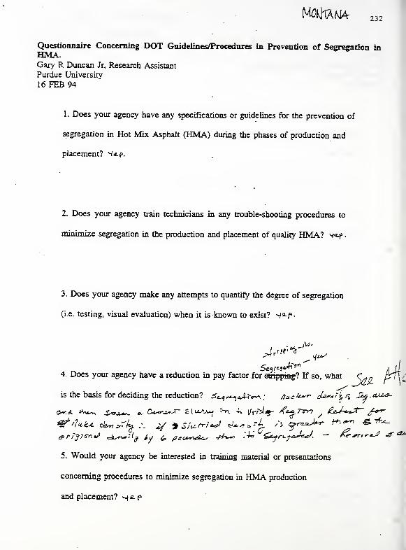
MOhAM* 232
Questionnaire Concerning DOT Guidelines/Procedures in Prevention of Segregation inHMA.Gary R Duncan Jr, Research Assistant
Purdue University
16 FEB 94
1. Does your agency have any specifications or guidelines for the prevention of
segregation in Hot Mix Asphalt (HMA) during the phases of production and
placement? s«.p.
2. Does your agency train technicians in any trouble-shooting procedures to
minimize segregation in the production and placement of quality HMA? v«-f
.
3. Does your agency make any attempts to quantify the degree of segregation
(i.e. testing, visual evaluation) when it is known to exist? ^s-f-
4. Does your agency have a reduction in pay factor for stripping? If so, what C^Q pTTf
is the basis for deciding the reduction? S*^i+^tev*\ \ Aaete*"* J***?^ SL&.clu^*-
4ffak* ok~,*rj^ ... tf *S/urr/*J *U«*?k Si ^toJ^r- ^~i &-*«-
5. Would your agency be interested in training material or presentations
concerning procedures to minimize segregation in HMA production
and placement? <-jji p
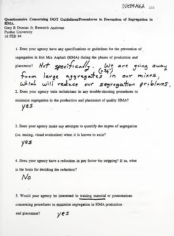
NWMft* 233
Questionnaire Concerning DOT Guidelines/Procedures in Prevention of Segregation in
HMA.Gary R Duncan Jr Research Assistant
Purdue University
16 FEB 94
1. Does your agency have any specifications or guidelines for the prevention of
segregation in Hot Mix Asphalt (HMA) during the phases of production and
placement? //?y KfiGcT'T'f C+~4'*i . (/J'C d>rt ^Ina CtujOLU
2. Does your agency train technicians in any trouble-shooting procedures to
minimize segregation in the production and placement of quality HMA?
yfi5
3. Does your agency make any attempts to quantify the degree of segregation
(i.e. testing, visual evaluation) when it is known to exist?
yes
4. Does your agency have a reduction in pay factor for stripping? If so, what
is the basis for deciding the reduction?
No
5. Would your agency be interested in training material or presentations
concerning procedures to minimize segregation in HMA production
and placement? \J g S
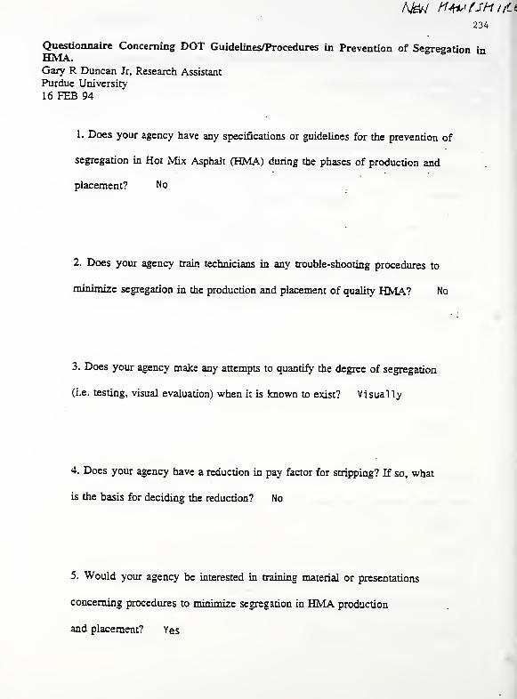
234
Questionnaire Concerning DOT Guidelines/Procedures in Prevention of Segregation inHMA. ^Gary R Duncan Jr, Research Assistant
Purdue University
16 FEB 94
1. Does your agency have any specifications or guidelines for the prevention of
segregation in Hot Mix Asphalt (HMA) during the phases of production and
placement? No
2. Does your agency train technicians in any trouble-shooting procedures to
minimize segregation in the production and placement of quality HMA? No
3. Does your agency make any attempts to quantify the degree of segregation
(i.e. testing, visual evaluation) when it is known to exist? Visually
4. Does your agency have a reduction in pay factor for stripping? If so, what
is the basis for deciding the reduction? No
5. Would your agency be interested in training material or presentations
concerning procedures to mimmize segregation in HMA production
and placement? Yes
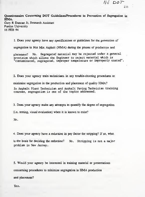
235
Questionnaire Concerning DOT Guidelines/Procedures in Prevention of Segregation in
HMA.Gary R Duncan Jr. Research Assistant
Purdue University
16 FEB 94
1. Does your agency have any specifications or guidelines for the prevention of
segregation in Hot Mix Asphalt (HMA) during the phases of production and
placement? No. Segregated material may be rejected under a general
provision which allows the Engineer to reject material which is
"contaminated, segregated, improper temperature or improperly coated".
2. Does your agency train technicians in any trouble-shooting procedures to
minimize segregation in the production and placement of quality HMA?
In Asphalt Plant Technician and Asphalt Paving Technician trainingcourses, segregation is one of the topics addressed.
3. Does your agency make any attempts to quantify the degree of segregation
(i.e. testing, visual evaluation) when it is known to exist?
No.
4. Does your agency have a reduction in pay factor for stripping? If so, what
is the basis for deciding the reduction? No. Stripping is not a major
problem in New Jersey.
5. Would your agency be interested in training material or presentations
concerning procedures to minimize segregation in HMA production
and placement?
Yes.

236
Questionnaire Concerning DOT Guidelines/Procedures in Prevention of Segregation inHMA.Gary R Duncan Jr. Research Assistant
Purdue University
16 FEB 94
1. Does your agency have any specifications or guidelines for the prevention of
segregation in Hot Mix Asphalt (HMA) during the phases of production and
placement? /^ ^^^£,^0. _S" >~>9
'
?-2Z-'Z7j£.'V/~~ y-yy,*??-
2. Does your agency train technicians in any trouble-shooting procedures to
m in imize segregation in the production and placement of quality HMA?
X&<> ,
3. Does your agency make any attempts to quantify the degree of segregation
(i.e. testing, visual evaluation) when it is known to exist? /}/£,
4. Does your agency have a reduction in pay factor for stripping? If so, what
is the basis for deciding the reduction? /Jra JT^.'s*ysy£- 'S
/Zf/Z x.y--^- 2 & /y rz^.f's~*
5. Would your agency be interested in training material or presentations
concerning procedures to minimize segregation in HMA production
and placement? s/s _? „
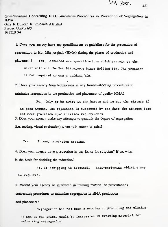
New Y<x^ 237
Questionnaire Concerning DOT Guidelines/Procedures in Prevention of Segregation in
HMA.Gary R Duncan Jr. Research Assistant
Purdue University
16 FEB 94
1. Does your agency have any specifications or guidelines for the prevention of
segregation in Hot Mix Asphalt (HMA) during the phases of production and
placement? Yes. Attached are specifications which pertain to the
mixer unit and the Hot Bituminous Mixer Holding Bin. The producer
is not required to own a holding bin.
2. Does your agency train technicians in any trouble-shooting procedures to
minimize segregation in the production and placement of quality HMA?
No. Only to be aware it can happen and reject the mixture if
it does happen. The rejection is supported by the fact the mixture does
not meet gradation specification requirements.
3. Does your agency make any attempts to quantify the degree of segregation
(i.e. testing, visual evaluation) when it is known to exist?
Yes Through gradation testing.
4. Does your agency have a reduction in pay factor for stripping? If so, what
is the basis for deciding the reduction?
No. If stripping is detected, anti-stripping additive may
be required.
5. Would your agency be interested in training material or presentations
concerning procedures to minimize segregation in HMA production
and placement?
Segregation has not been a problem in producing and placing
of HMA in the state. Would be interested in training material for
minimizing segregation.
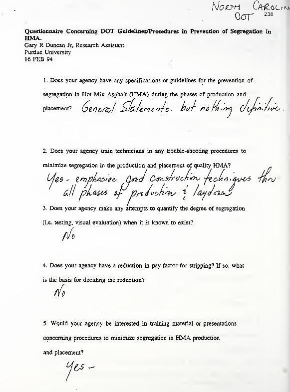
Oct 238
Questionnaire Concerning DOT Guidelines/Procedures in Prevention of Segregation in
HMA.Gary R Duncan Jr, Research Assistant
Purdue University
16 FEB 94
1. Does your agency have any specifications or guidelines for the prevention of
segregation in Hot Mix Asphalt (HMA) during the phases of production and
placement? OlOLfcl $>fasfCULT'S &0T nOfh'^ ULf'^'T*^
2. Does your agency train technicians in any trouble-shooting procedures to
minimize segregation in the production and placement of quality HMA?
3. Does your agency make any attempts to quantify the degree of segregation
(i.e. testing, visual evaluation) when it is known to exist?
fit
4. Does your agency have a reduction in pay factor for stripping? If so, what
is the basis for deciding the reduction?
do
5. Would your agency be interested in training material or presentations
concerning procedures to minimise segregation in HMA production
and placement?
ru
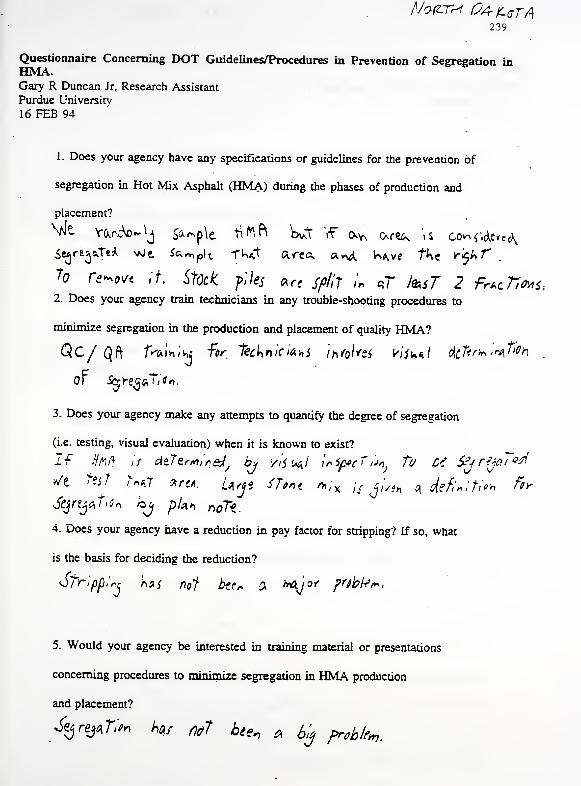
N?(LTH Oa-uta239
Questionnaire Concerning DOT Guidelines/Procedures in Prevention of Segregation inHMA.Gary R Duncan Jr. Research Assistant
Purdue University
16 FEB 94
1. Does your agency have any specifications or guidelines for the prevention of
segregation in Hot Mix Asphalt (HMA) during the phases of production and
placement?
£e^r»^«TtA wt ^^ pl t rUfl" area, a^ ^vc Ac ^f
,
to re^ovt it. Stock f'M *ct split in sT J&sT 2 fhc77*is-.2. Does your agency train technicians in any trouble-shooting procedures to
minimize segregation in the production and placement of quality HMA?
Qc/ Qft f^ihiw "fir technicians it\fol*ei vi$w*\ dcT^r^.^t'Om
of Serre^sJiSn.
3. Does your agency make any attempts to quantify the degree of segregation
(i.e. testing, visual evaluation) when it is known to exist?
If tihft if deters,'nedy
bj sis <*l i»Sp*cT ,'j^ fu C{ $?j rfjaTed
v/l ItsT fMT firiA. Urji i7##»« m,\\s j/,f„ q fafinlti** fir
4. Does your agency have a reduction in pay factor for stripping? if so, what
is the basis for deciding the reduction?
^Stripp.'rr nfi$ nof btr* a htijof ?rsbtet».
5. Would your agency be interested in training material or presentations
concerning procedures to minimize segregation in HMA production
and placement?
Sejrej^r:^ ha/ not bie« *fy Fr hlf^.

OHIO DOT240
Questionnaire Concerning DOT Guidelmes/Procedures in Prevention of Segregation in
Gary R Duncan Jr. Research Assistant
Purdue University
16 FEB 94
1. Does your agency have any specifications or guidelines for the prevention of
segregation in Hot Mix Asphalt (HMA) during the phases of production and
placement? OiJ^ ^SuC*J^ OS p 1&L€£) or^S ooJ^lK-frudL ioc^
2. Does your agency train technicians in any trouble-shooting procedures to
minimize segregation in the production and placement of quality HMA?
3. Does your agency make any attempts to quantify the degree of segregation
(i.e. testing, visual evaluation) when it is known to exist?
4. Does your agency have a reduction in pay factor for stripping? If so, what
is the basis for deciding the reduction? S/'O
5. Would your agency be interested in training material or presentations
concerning procedures to minimize segregation in HMA production
and placement? Sjo O^on^ol^C^)^ (XJo^ o{ ik \fOTtOOS

241
Questionnaire Concerning DOT Giudelines/Procedures in Prevention of Segregation inHMA.Gary R Duncan Jr. Research Assistant
Purdue University
16 FEB 94
1. Does your agency have any specifications or guidelines for the prevention of
segregation in Hot Mix Asphalt (HMA) during the phases of production and
placement? $f>eC f> C& f•*^> £T#&5
" SeSfagfiTrc?* erf The. m;*r«re win nor be acceffckle.
2. Does your agency train technicians in any trouble-shooting procedures to
minimize segregation in the production and placement of quality HMA?^C3 in &nf0,-nf cic<$se5
3. Does your agency make any attempts to quantify the degree of segregation
(i.e. testing, visual evaluation) when it is known to exist?
i/t 'Sue* ' 6i/& hj&r> '0*^
4. Does your agency have a reduction in pay factor for stripping? If so, what
is the basis for deciding the reduction? A/fl
we c/t? h#*e. & $u;rt>»J TesT 6,'*"'/<*' ~^
flfiSH-Tc? T-Z&3 useJ T<? cJeTer^>ne.
5. Would your agency be interested in training material or presentations
concerning procedures to minimize segregation in HMA production
and placement? #-735 /J, / y
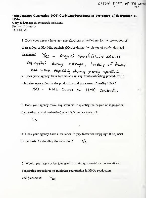
ORCGOiJ D6PH oT TRA^Psb242
Questionnaire Concerning DOT Guidelines/Procedures in Prevention of Segregation in
HMA.Gary R Duncan Jr. Research Assistant
Purdue University
16 FEB 94
1. Does your agency have any specifications or guidelines for the prevention of
segregation in Hot Mix Asphalt (HMA) during the phases of production and
placement? ^ _ ^^; Sf*«£c«i^f QdcircS
S
2. Does your agency train technicians in any trouble-shooting procedures to
minimise segregation in the production and placement of quality HMA?
Yes - H)Al Course. 0vv 14*4 Consfacfc
3. Does your agency make any attempts to quantify the degree of segregation
(i.e. testing, visual evaluation) when it is known to exist?
4. Does your agency have a reduction in pay factor for stripping? If so, what
is the basis for deciding the reduction? f^o.
5. Would your agency be interested in training material or presentations
concerning procedures to minimize segregation in HMA production
and placement? Y&S
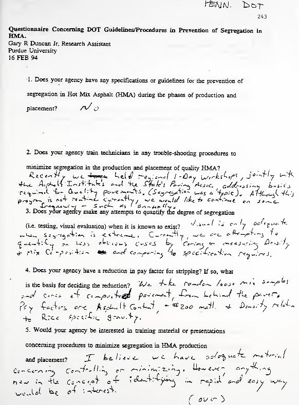
243
Questionnaire Concerning DOT Guidelines/Procedures in Prevention of Segregation inHMA.Gary R Duncan Jr, Research Assistant
Purdue University
16 FEB 94
1. Does your agency have any specifications or guidelines for the prevention of
segregation in Hot Mix Asphalt (HMA) during the phases of production and
placement? /^ O
2. Does your agency train technicians in any trouble-shooting procedures to
minimize segregation in the production and placement of quality HMA?^c^^v u,c-tHP«. kdrf r-et:*~*i I -Cay \s/,rksLfi j J f'-J-ly t~i<s
*f-Ui. At/^tVX^X+'+^Wi e^A 'fU 1%^'j P+*}~^ Ass*C. G*tdk'±Si-<H i-i^'j
3. Does your agency make any attempts to quantify the degree of segregation
(i.e. testing, visual evaluation) when it is known to exist?,/ ^"*< ,J c 'v
y0c '$**'
4. Does your agency have a reduction in pay factor for stripping? If so, what
is the basis for deciding the reduction? ^^ T^ « r*>-.«/w /ooj« /*»»« **-y° J
5. Would your agency be interested in training material or presentations
concerning procedures to ininimize segregation in HMA production
andplacement? X U I i «-•*, w * A*„ c r<^-^ ^W>
j r • j -I i •• •
/(/
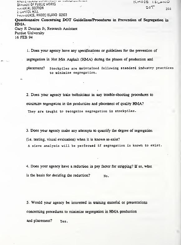
DlvioiU.i Of PUBLIC WORKS '"" "^
K,A i tKIAL SECTION C>o \ 2442 CAr'ifOL HILL
Kku«.D£NCE, RHODE ISLAND 02903
Questionnaire Concerning DOT Guidelines/Procedures in Prevention of Segregation in
HMA.Gary R Duncan Jr, Research Assistant
Purdue University
16 FEB 94
1. Does your agency have any specifications or guidelines for the prevention of
segregation in Hot Mix Asphalt (HMA) during the phases of production and
placement? Stockpiles are maintained following standard industry practices
to minimize segregation.
2. Does your agency train technicians in any trouble-shooting procedures to
minimize segregation in the production and placement of quality HMA?
They are taught to recognize segregation in stockpiles.
3. Does your agency make any attempts to quantify the degree of segregation
(i.e. testing, visual evaluation) when it is known to exist?
A sieve analysis will be performed if segregation is known to exist.
4. Does your agency have a reduction in pay factor for stripping? If so, what
is the basis for deciding the reduction? No
.
5. Would your agency be interested in training material or presentations
concerning procedures to minimize segregation in HMA production
and placement? ye s.
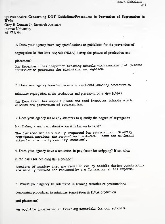
SOUTH CAROLINA245
Questionnaire Concerning DOT Guidelines/Procedures in Prevention of Segregation in
HMA.Gary R Duncan Jr, Research Assistant
Purdue University
16 FEB 94
1. Does your agency have any specifications or guidelines for the prevention of
segregation in Hot Mix Asphalt (HMA) during the phases of production and
placement?
Our Department has inspector training schools with manuals that discuss
construction practices for minimizing segregation.
2. Does your agency train technicians in any trouble-shooting procedures to
minimize segregation in the production and placement of quality HMA?
Our Department has asphalt plant and road inspector schools which
discuss the prevention of segregation.
3. Does your agency make any attempts to quantify the degree of segregation
(i.e. testing, visual evaluation) when it is known to exist?
The finished mat is visually inspected for segregation. Severely
segregated sections are removed and replaced. There are no formal
attempts to actually quantify (measure).
4. Does your agency have a reduction in pay factor for stripping? If so, what
is the basis for deciding the reduction?
Sections of roadway that are ravelled out by traffic during construction
are usually removed and replaced by the Contractor at his expense.
5. Would your agency be interested in training material or presentations
concerning procedures to niinimize segregation in HMA production
and placement?
We would be interested in training materials for our schools.
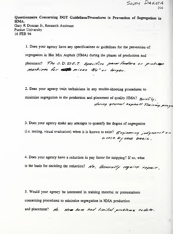
South D+Z-otA246
Questionnaire Concerning DOT Guidelines/Procedures in Prevention of Segregation inHMA.Gary R Duncan Jr. Research Assistant
Purdue University
16 FEB 94
1. Does your agency have any specifications or guidelines for the prevention of
segregation in Hot Mix Asphalt (HMA) during the phases of production and
placement? 7/*<? S. D. Z20. 7~. ^fxgcr/Crs /="****' /ZrtnSs's-s *s ^>^^-^o/f7tt<f6/sf'S &s- 2fl$£ /nS*4*s c^"„^ Aa^fiSy.
2. Does your agency train technicians in any trouble-shooting procedures to
minimize segregation in the production and placement of quality HMA? Bri-
<o£7
y,
c/ury^f ?<*„*>**/ osf>/,a/* 7^/^*^^^
3. Does your agency make any attempts to quantify the degree of segregation
(i.e. testing, visual evaluation) when it is known to exist? ^y/^ww™ J,*/****^/*& £0^e. &>y case &&S/S. .
4. Does your agency have a reduction in pay factor for stripping? If so, what
is the basis for deciding the reduction? /^ &<**<>,<*//?> ray"^ rr/=*a,^
5. Would your agency be interested in training material or presentations
concerning procedures to minimize segregation in HMA production
and placement? //a. */*>— Aa*z S?ac//>»*//<-*/
fp^S/e^* ^etafe
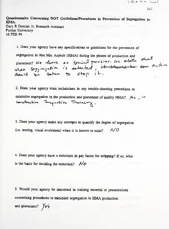
A ^ l ~ '~^> T
247
Questionnaire Concerning DOT Guidelines/Procedures in Prevention of Segregation inHMA.Gary R Duncan Jr. Research Assistant
Purdue University
16 FEB 94
1. Does your agency have any specifications or guidelines for the prevention of
segregation in Hot Mix Asphalt (HMA) during the phases of production and »
placement? A/e -bw<- k« 5,^-J? f~"*«"«*<• U<~ *4^'A J-
2. Does your agency train technicians in any trouble-shooting procedures to
minimize segregation in the production and placement of quality HMA? /*% , i*
3. Does your agency make any attempts to quantify the degree of segregation
(i.e. testing, visual evaluation) when it is known to exist? A/0
4. Does your agency have a reduction in pay factor for stripping? if so, what
is the basis for deciding the reduction? NO
5. Would your agency be interested in training material or presentations
concerning procedures to minimize segregation in HMA production
and placement? ye*?

243
Questionnaire Concerning DOT Guidelines/Procedures in Prevention of Segregation in
HMA.Gary R Duncan Jr, Research Assistant
Purdue University
16 FEB 94
1. Does your agency have any specifications or guidelines for the prevention of
segregation in Hot Mix Asphalt (HMA) during the phases of production and
placement? — 7t<? , /*&S -4pc£lte£ &^£ .
2. Does your agency train technicians in any trouble-shooting procedures to
minimize segregation in the production and placement of quality HMA? —$0>*JL J^t^J. s>ud- a>6 <U-^ —»*c^ w^£> ~4-Ji4«m£ -£c
3. Does your agency make any attempts to quantify the degree of segregation
(i.e. testing, visual evaluation) when it is known to exist? -
—*<*
4. Does your agency have a reduction in pay factor for stripping? If so, what
is the basis for deciding the reduction? — ***^
5. Would your agency be interested in training material or presentations
concerning procedures to minimize segregation in HMA production
and placement? _ u^a* -
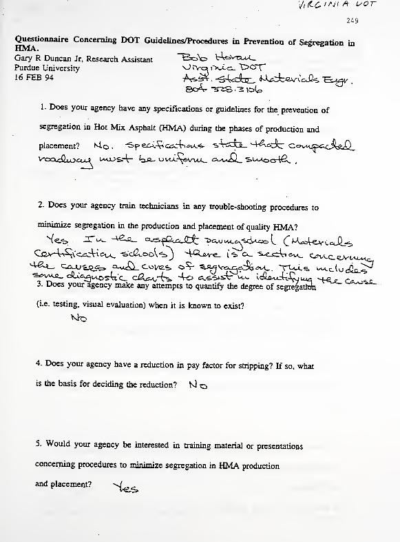
\ji<Lc.iN[ fit uor
249
Questionnaire Concerning DOT Guidelines/Procedures in Prevention of Segregation in
Gary R Duncan Jr, Research Assistant "Bob b-Wv-ccU^
Purdue University \J\V<=» ixic ~D>CS"X~
16 FEB 94 A^ . ^c&x_ UtfdbavCcJk "B^v .
1. Does your agency have any specifications or guidelines for the prevention of
segregation in Hot Mix Asphalt (HMA) during the phases of production and
placement? Nio . "SpecjL-^osc^^x^ •sAcCO- '-l&cck: 0<^v^ffx=<JW<Q_
2. Does your agency train technicians in any trouble-shooting procedures to
minimize segregation in the production and placement of quality HMA?
3. Does your agency make any attempts to quantify the degree of segregation«*^**-
(i.e. testing, visual evaluation) when it is known to exist?
4. Does your agency have a reduction in pay factor for stripping? If so, what
is the basis for deciding the reduction? NJ o
5. Would your agency be interested in training material or presentations
concerning procedures to minimize segregation in HMA production
and placement? v/ .
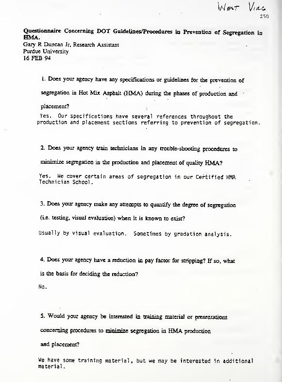
W^r \Jiilc
250
Questionnaire Concerning DOT Guidelines/Procedures in Prevention of Segregation inHMA.
e s
Gary R Duncan Jr. Research Assistant
Purdue University
16 FEB 94
1. Does your agency have any specifications or guidelines for the prevention of
segregation in Hot Mix Asphalt (HMA) during the phases of production and
placement?
Yes. Our specifications have several references throughoat theproduction and placement sections referring to prevention of segregation.
2. Does your agency train technicians in any trouble-shooting procedures to
minimize segregation in the production and placement of quality HMA?
Yes. We cover certain areas of segregation in our Certified HMATechnician School
.
3. Does your agency make any attempts to quantify the degree of segregation
(i.e. testing, visual evaluation) when it is known to exist?
Usually by visual evaluation. Sometimes by gradation analysis.
4. Does your agency have a reduction in pay factor for stripping? If so, what
is the basis for deciding the reduction?
No.
5. Would your agency be interested in training material or presentations
concerning procedures to minimi** segregation in HMA production
and placement?
We have some training material, but we may be interested in additionalmaterial
.
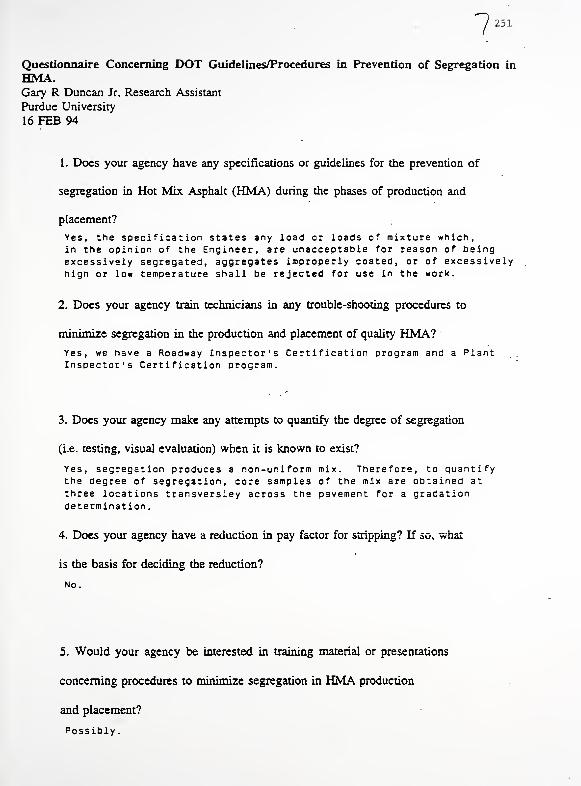
7 251
Questionnaire Concerning DOT Guidelines/Procedures in Prevention of Segregation in
HMA.Gary R Duncan Jr. Research Assistant
Purdue University
16 FEB 94
1. Does your agency have any specifications or guidelines for the prevention of
segregation in Hot Mix Asphalt (HMA) during the phases of production and
placement?
Yes, the specification states any load or loads of mixture which,in the opinion of the Engineer, are unacceptable for reason of beingexcessively segregated, aggregates improperly coated, or of excessivelyhigh or low temperature shall be rejected for use in the work.
2. Does your agency train technicians in any trouble-shooting procedures to
minimize segregation in the production and placement of quality HMA?Yes, we have a Roadway Inspector's Certification program and a PlantInspector's Certification program.
3. Does your agency make any attempts to quantify the degree of segregation
(i.e. testing, visual evaluation) when it is known to exist?
Yes, segregation produces a non-uniform mix. Therefore, to quantifythe degree of segregation, core samples of the mix are obtained at
three locations transversley across the pavement for a gradationdetermination
.
4. Does your agency have a reduction in pay factor for stripping? If so, what
is the basis for deciding the reduction?
No.
5. Would your agency be interested in training material or presentations
concerning procedures to minimize segregation in HMA production
and placement?
Possibly.

252
APPENDIX BTraining Video Script

25:
Properly designed, produced and placed Hot Mix Asphalt provides durable, long
lasting pavements, requiring little maintenance. Yet segregation of these mixtures has
caused problems in the paving industry. Problems that can be avoided
Segregation is a process which results in a non-uniform aggregate stockpile, gradation or
HMA mix that contains concentrated areas of fine and coarse aggregate Segregated
HMA mixes do not perform the way they are designed.
Fine areas of the segregated HMA hold the majority of the asphalt in the mix, which
makes them over rich with asphalt, have low air voids and a tendency to rut and shove
Coarse areas of a segregated HMA are deficient in asphalt and lack the fine mastic to
hold the larger, coarse aggregate in place, which may lead to ravelling Coarse areas are
also more permeable, allowing water to enter the pavement which could cause stripping
of the mat.
We are going to show you the five steps of the HMA production and construction
processes where segregation can occur. They are mix design production and
stockpiling of aggregate HMA manufacturing and storage facilities truck loading
and transfer and paving.
Segregation can be reduced considerably by properly designing the mix. Mixes that are
well designed tend to be more forgiving and allow for mistakes in HMA construction
Gap graded mixes should be avoided since they are unforgiving and at low asphalt
contents usually can not be produced without segregation, regardless of the equipment or
techniques used.
The maximum density curve can be a guide to ensure proper mix design. A gradation
that falls directly on the maximum density curve should not be used since it would leave
insufficient room for the asphalt. The designer should select two to four percentage
points above the curve for a finer texture. For a coarser texture, select two to four
percentage points below the curve. A grading curve that roughly parallels the maximumdensity line will produce uniformly graded mixes that are more forgiving. However, the
maximum density curve should only be used as a guide for mix design and density. Other
criteria, such as air voids, VMA and stability are also important.
Proper stockpiling techniques will help ensure that uniform materials are being supplied
to the HMA manufacturing facility. In a conical stockpile .... segregation will occur
because the larger stones tend to roll down the sides and to the outside of the pile. If this
occurs, segregated materials will be fed to the mix plant unless they are remixed
beforehand.
When constructing stockpiles with trucks, the aggregate should be piled in units not
larger than a single truckload and no higher than one layer of truckloads.
When using a crane or a bucket, the loads should be deposited adjacent to and
overlapping one another to form a layer of uniform thickness.
Stockpiles should be built in progressive, horizontal layers.
When a conveyor is used, a bulldozer should be used to distribute the pile in horizontal
layers to keep the aggregate from forming a conical pile.
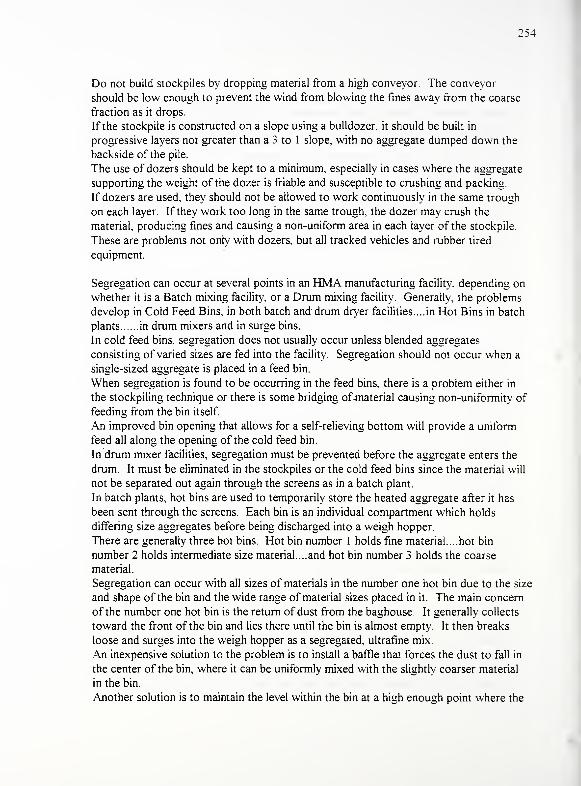
254
Do not build stockpiles by dropping material from a high conveyor. The conveyor
should be low enough to prevent the wind from blowing the fines away from the coarse
fraction as it drops.
If the stockpile is constructed on a slope using a bulldozer, it should be built in
progressive layers not greater than a 3 to 1 slope, with no aggregate dumped down the
backside of the pile.
The use of dozers should be kept to a minimum, especially in cases where the aggregate
supporting the weight of the dozer is friable and susceptible to crushing and packing.
If dozers are used, they should not be allowed to work continuously in the same trough
on each layer. If they work too long in the same trough, the dozer may crush the
material, producing fines and causing a non-uniform area in each layer of the stockpile.
These are problems not only with dozers, but all tracked vehicles and rubber tired
equipment.
Segregation can occur at several points in an HMA manufacturing facility, depending on
whether it is a Batch mixing facility, or a Drum mixing facility. Generally, the problems
develop in Cold Feed Bins, in both batch and drum dryer facilities... in Hot Bins in batch
plants in drum mixers and in surge bins.
In cold feed bins, segregation does not usually occur unless blended aggregates
consisting of varied sizes are fed into the facility. Segregation should not occur when a
single-sized aggregate is placed in a feed bin.
When segregation is found to be occurring in the feed bins, there is a problem either in
the stockpiling technique or there is some bridging of-material causing non-uniformity of
feeding from the bin itself.
An improved bin opening that allows for a self-relieving bottom will provide a uniform
feed all along the opening of the cold feed bin.
In drum mixer facilities, segregation must be prevented before the aggregate enters the
drum. It must be eliminated in the stockpiles or the cold feed bins since the material will
not be separated out again through the screens as in a batch plant.
In batch plants, hot bins are used to temporarily store the heated aggregate after it has
been sent through the screens. Each bin is an individual compartment which holds
differing size aggregates before being discharged into a weigh hopper
There are generally three hot bins. Hot bin number 1 holds fine material....hot bin
number 2 holds intermediate size material.... and hot bin number 3 holds the coarse
material.
Segregation can occur with all sizes of materials in the number one hot bin due to the size
and shape of the bin and the wide range of material sizes placed in it. The main concern
of the number one hot bin is the return of dust from the baghouse. It generally collects
toward the front of the bin and lies there until the bin is almost empty. It then breaks
loose and surges into the weigh hopper as a segregated, ultrafine mix.
An inexpensive solution to the problem is to install a baffle that forces the dust to fall in
the center of the bin, where it can be uniformly mixed with the slightly coarser material
in the bin.
Another solution is to maintain the level within the bin at a high enough point where the
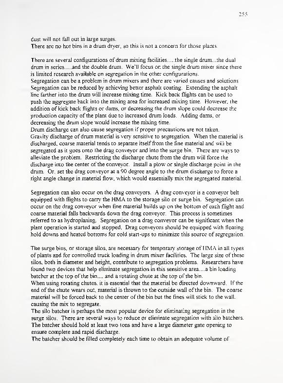
255
dust will not fall out in large surges.
There are no hot bins in a drum dryer, so this is not a concern for those plants
There are several configurations of drum mixing facilities the single drum the dual
drum in series and the double drum. We'll focus on the single drum mixer since there
is limited research available on segregation in the other configurations
Segregation can be a problem in drum mixers and there are varied causes and solutions
Segregation can be reduced by achieving better asphalt coating. Extending the asphalt
line farther into the drum will increase mixing time. Kick back flights can be used to
push the aggregate back into the mixing area for increased mixing time. However, the
addition of kick back flights or dams, or decreasing the drum slope could decrease the
production capacity of the plant due to increased drum loads. Adding dams, or
decreasing the drum slope would increase the mixing time.
Drum discharge can also cause segregation if proper precautions are not taken.
Gravity discharge of drum material is very sensitive to segregation. When the material is
discharged, coarse material tends to separate itself from the fine material and will be
segregated as it goes onto the drag conveyor and into the surge bin. There are ways to
alleviate the problem. Restricting the discharge chute from the drum will force the
discharge into the center of the conveyor. Install a plow or single discharge point in the
drum. Or, set the drag conveyor at a 90 degree angle to the drum discharge to force a
right angle change in material flow, which would essentially mix the segregated material
Segregation can also occur on the drag conveyors. A drag conveyor is a conveyor belt
equipped with flights to carry the HMA to the storage silo or surge bin. Segregation can
occur on the drag conveyor when fine material builds up on the bottom of each flight and
coarse material falls backwards down the drag conveyor. This process is sometimes
referred to as hydroplaning. Segregation on a drag conveyor can be significant when the
plant operation is started and stopped. Drag conveyors should be equipped with floating
hold downs and heated bottoms for cold start-ups to minimize this source of segregation.
The surge bins, or storage silos, are necessary for temporary storage ofHMA in all types
of plants and for controlled truck loading in drum mixer facilities. The large size of these
silos, both in diameter and height, contribute to segregation problems. Researchers have
found two devices that help eliminate segregation in this sensitive area... a bin loading
batcher at the top of the bin and a rotating chute at the top of the bin.
When using rotating chutes, it is essential that the material be directed downward. If the
end of the chute wears out, material is thrown to the outside wall of the bin. The coarse
material will be forced back to the center of the bin but the fines will stick to the wall.
causing the mix to segregate.
The silo batcher is perhaps the most popular device for eliminating segregation in the
surge silos. There are several ways to reduce or eliminate segregation with silo batchers.
The batcher should hold at least two tons and have a large diameter gate opening to
ensure complete and rapid discharge.
The batcher should be filled completely each time to obtain an adequate volume of
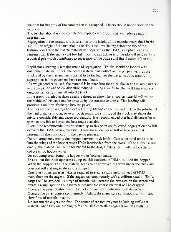
256
material for integrity of the batch when it is dropped. Timers should not be used on the
batchers.
The batcher should not be completely emptied each drop. This will reduce random
segregation.
Segregation in the storage silo is sensitive to the height of the material maintained in the
silo. If the height of the material in the silo is too low (falling below the top of the
bottom cone) then the coarse material will separate as the HMA is emptied, causing
segregation. If the silo is kept too full, then the mix falling into the silo will tend to form
a conical pile which contributes to separation of the coarse and fine fraction of the mix
Rapid truck loading is a major cause of segregation. Trucks should be loaded with
distributed batches. If not, the coarse material will collect on the outside walls of the
truck and be the first and last material to be loaded into the paver, causing areas of
segregation in the pavement between truck loads.
If a weigh batcher is used, the material is batched into the truck similar to the silo batcher
and segregation can be considerably reduced. Using a weigh batcher will help ensure a
uniform transfer of material into the truck.
If the truck is loaded in three separate drops, as shown here, coarse material will roll to
the middle of the truck and be covered by the successive drops. This loading will
promote a uniform discharge into the paver.
Another source of segregation occurs during hauling of the mix by truck to thejobsite. If
the haul distance is long, or over rough roads, the stiff ride of the truck may shake the
mixture considerably and cause segregation. It is recommended that haul distances be as
short as possible and over the best roads available.
Even if the recommendations presented up to this point are followed, segregation can still
occur in the HMA paving machine. There are guidelines to follow to ensure that
segregation does not occur in the paving process.
Do not completely empty the hopper between truck loads. Coarse material tends to roll
into the wings of the hopper when HMA is unloaded from the truck. If the hopper is not
empty, the material will be uniformly fed to the drag flights since it will not be able to
collect in the hopper wings.
Do not completely dump the hopper wings between loads.
Ensure that the truck operators dump the full truckload ofHMA to flood the hopper.
When the hopper is full, the material tends to be conveyed out from under the truck and
does not roll and segregate as it is dumped.
Open the hopper gates as wide as required to ensure that a uniform head ofHMA is
maintained on the augers. If the augers run continuously with a uniform head ofHMAsurges will be avoided. A surge of material will increase the pressure on the screed and
create a rough spot on the pavement because the coarse material will be dragged.
Operate the paver continuously. Do not stop and start between truck deliveries.
Operate the paver augers continuously Adjust the speed so a continuous, uniform and
slow flow of material occurs.
Do not run the augers too fast. The center of the mat may not be holding sufficient
material when they are running to fast, causing centerline segregation. If a baffle is
257
installed, the augers in the flights will kick uniform material back to the center.
Alternate paving procedures include material transfer vehicles which can be used to load
material into the hopper
One alternative paving procedure that has been found to reduce segregation involves
laying down a windrow in front of the paver rather than dumping the mix directly into the
hopper.
The transfer vehicle picks up the HMA from the windrow with paddles, slightly mixing
the HMA, then delivers it to a hopper with increased capacity. This process is
continuous, which is beneficial since the HMA is slightly remixed and the hopper is
never emptied. Segregation caused by improper truck loading, improper transfer to the
hopper or improper hopper use could be eliminated.
Another procedure involves a transfer vehicle which has an insulated surge bin with an
auger that remixes the HMA before delivering it to the hopper. The truck dumps directly
into the transfer vehicle, rather than placing it in a windrow in front of the paver It is
also a continuous process with the same benefits of the windrow, except the HMA is
mixed more efficiently, resulting in a more uniform pavement.
These guidelines should minimize segregation in the production and laydown of Hot Mix
Asphalt pavements. If the recommendations for proper mix design proper operation of
the HMA manufacturing facility truck loading and paving operations are followed.
segregation should be reduced, hopefully eliminated.
258
APPENDIX CSequence of Steps to Establish Correction Factors
259
This appendix contains the results of the SAS analysis of the correction factors
established for nuclear density and asphalt content. The correction factors were
established as follows:
1
.
Four, one minute readings of density and asphalt content were taken on each
sample.
2. These readings were averaged.
3. The average was then compared to known values of density and asphalt
content and a correction factor was established for each observation.
The General Linear Model (GLM) procedure was then used to analyze these data. The
GLM procedure was used to:
4. Determine the significance of each class (independent factor) to the model.
Insignificant factors were dropped from the GLM model. The results
contained in this Appendix reflect only the factors that were significant to the
model. The discussion of these significant factors is contained in Sections
5.2.4 and 5.2.5.
5. Group the data at 95% confidence as outlined in Tables A.7, A.8, A. 1 8-A.20.
The groupings were necessary to identify individual groupings that could
require different correction factors (i.e. DOS for Asphalt Content or
MLXTYPE for Density).
6. Fit a model of the correction factors and establish a 95% upper and lower
confidence interval. These data are contained in Tables A. 10 and A.23.
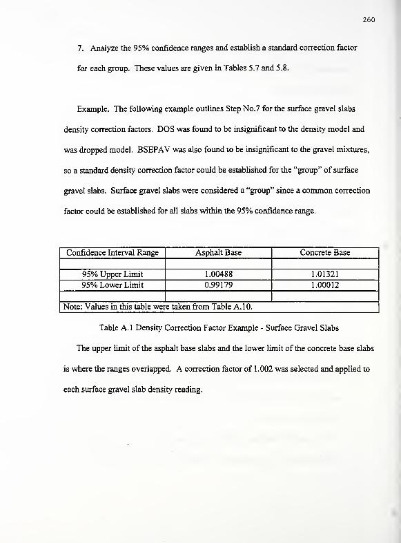
260
7. Analyze the 95% confidence ranges and establish a standard correction factor
for each group. These values are given in Tables 5.7 and 5.8.
Example. The following example outlines Step No.7 for the surface gravel slabs
density correction factors. DOS was found to be insignificant to the density model and
was dropped model. BSEPAV was also found to be insignificant to the gravel mixtures,
so a standard density correction factor could be established for the "group" of surface
gravel slabs. Surface gravel slabs were considered a "group" since a common correction
factor could be established for all slabs within the 95% confidence range.
Confidence Interval Range Asphalt Base Concrete Base
95% Upper Limit 1.00488 1.01321
95% Lower Limit 0.99179 1.00012
Note: Values in this table were taken from Table A. 10.
Table A.l Density Correction Factor Example - Surface Gravel Slabs
The upper limit of the asphalt base slabs and the lower limit of the concrete base slabs
is where the ranges overlapped. A correction factor of 1 .002 was selected and applied to
each surface gravel slab density reading.
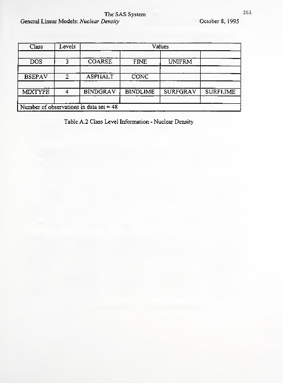
The SAS System
General Linear Models: Nuclear Density
261
October 8, 1995
Class Levels Values
DOS 3 COARSE FINE UNIFRM
BSEPAV 2 ASPHALT CONC
MIXTYPE 4 BINDGRAV BINDLIME SURFGRAV SURFLIME
Number of observations in data set = 48
Table A.2 Class Level Information - Nuclear Density
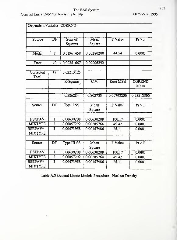
The SAS System
General Linear Models: Nuclear Density
262
October 8, 1995
Dependent Variable: CORRND
Source DF Sum of
Squares
MeanSquare
F Value Pr>F
Model 7 0.01961458 0.00280208 44.54 0.0001
Error 40 0.00251667 0.00006292
Corrected
Total
47 0.02213125
R-Square C.V. Root MSE CORRNDMean
0.886284 0.802733 0.00793200 0.98812500
Source DF Type I SS MeanSquare
F Value Pr>F
BSEPAV 1 0.00630208 0.00630208 100.17 0.0001
MIXTYPE 3 0.00857292 0.00285764 45.42 0.0001
BSEPAV*MIXTYPE
3 0.00473958 0.00157986 25.11 0.0001
Source DF Type III SS MeanSquare
F Value Pr>F
BSEPAV 1 0.00630208 0.00630208 100.17 0.0001
MIXTYPE 3 0.00857292 0.00285764 45.42 0.0001
BSEPAV*MIXTYPE
3 0.00473958 0.00157986 25.11 0.0001
Table A.3 General Linear Models Procedure - Nuclear Density
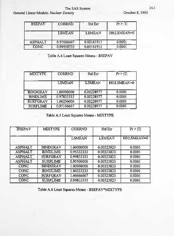
The SAS System
General Linear Models: Nuclear Density
263
October 8, 1995
BSEPAV CORRND StdErr Pr>|T|
LSMEAN LSMEAN H0:LSMEAN=0
ASPHALT 0.97666667 0.00161911 0.0001
CONC 0.99958333 0.00161911 0.0001
Table A.4 Least Squares Means - BSEPAV
MIXTYPE CORRND StdErr Pr>|T|
LSMEAN LSMEAN H0:LSMEAN=0
BINDGRAV 1.00000000 0.00228977 0.0001
BINDLIME 0.97833333 0.00228977 0.0001
SURFGRAV 1.00250000 0.00228977 0.0001
SURFLIME 0.97166667 0.00228977 0.0001
Table A.5 Least Squares Means - MIXTYPE
BSEPAV MIXTYPE CORRND StdErr Pr > |T|
LSMEAN LSMEAN H0:LSMEAN=0
ASPHALT BINDGRAV 1.00000000 0.00323823 0.0001
ASPHALT BINDLIME 0.95333333 0.00323823 0.0001
ASPHALT SURFGRAV 0.99833333 0.00323823 0.0001
ASPHALT SURFLIME 0.95500000 0.00323823 0.0001
CONC BINDGRAV 1.00000000 0.00323823 0.0001
CONC BINDLIME 1.00333333 0.00323823 0.0001
CONC SURFGRAV 1.00666667 0.00323823 0.0001
CONC SURFLIME 0.99833333 0.00323823 0.0001
Table A.6 Least Squares Means - BSEPAV*MLXTYPE
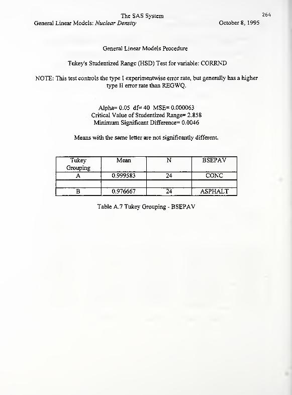
The SAS System
General Linear Models: Nuclear Density
264
October 8, 1995
General Linear Models Procedure
Tukey's Studentized Range (HSD) Test for variable: CORRND
NOTE: This test controls the type I experimentwise error rate, but generally has a higher
type II error rate than REGWQ.
Alpha=0.05 df=40 MSE= 0.000063
Critical Value of Studentized Range= 2.858
Minimum Significant Difference= 0.0046
Means with the same letter are not significantly different.
Tukey
Grouping
Mean N BSEPAV
A 0.999583 24 CONC
B 0.976667 24 ASPHALT
Table A.7 Tukey Grouping - BSEPAV
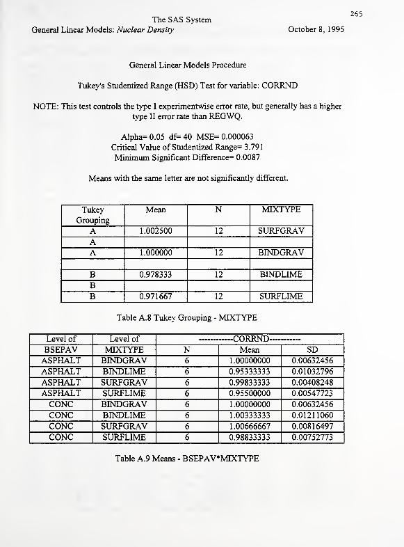
The SAS System
General Linear Models: Nuclear Density
265
October 8, 1995
General Linear Models Procedure
Tukey's Studentized Range (HSD) Test for variable: CORRND
NOTE: This test controls the type I experimentwise error rate, but generally has a higher
type II error rate than REGWQ.
Alpha= 0.05 df= 40 MSE= 0.000063
Critical Value of Studentized Range= 3.791
Minimum Significant Difference= 0.0087
Means with the same letter are not significantly different.
Tukey
Grouping
Mean N MIXTYPE
A 1.002500 12 SURFGRAVAA 1.000000 12 BINDGRAV
B 0.978333 12 BINDLIMEBB 0.971667 12 SURFLIME
Table A. 8 Tukey Grouping - MIXTYPE
Level of Level of . „ rORRND -
BSEPAV MIXTYPE N Mean SDASPHALT BINDGRAV 6 1.00000000 0.00632456
ASPHALT BINDLIME 6 0.95333333 0.01032796
ASPHALT SURFGRAV 6 0.99833333 0.00408248
ASPHALT SURFLIME 6 0.95500000 0.00547723
CONC BINDGRAV 6 1.00000000 0.00632456
CONC BINDLIME 6 1.00333333 0.01211060
CONC SURFGRAV 6 1.00666667 0.00816497
CONC SURFLIME 6 0.98833333 0.00752773
Table A.9 Means - BSEPAV*MIXTYPE
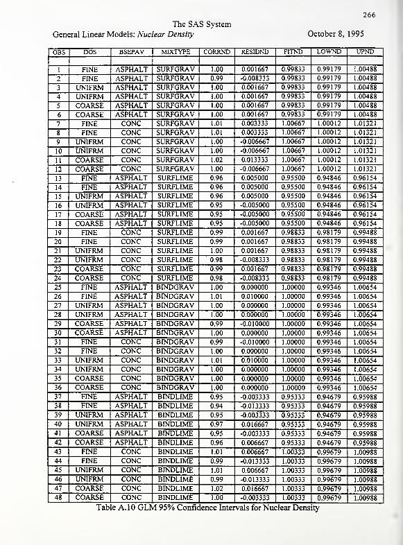
The SAS System
General Linear Models: Nuclear Density
266
October 8, 1995
OBS DOS BSEPAV MIXTYPE CORRND RESIDND FITND LOWND UPND
1 FrNE ASPHALT SURFGRAV 1.00 0.001667 0.99833 0.99179 1.00488
2 FINE ASPHALT SURFGRAV 0.99 -0.008333 0.99833 0.99179 1.00488
3 UNIFRM ASPHALT SURFGRAV 1.00 0.001667 0.99833 0.99179 1.00488
4 UNIFRM ASPHALT SURFGRAV 1.00 0.001667 0.99833 0.99179 1.00488
5 COARSE ASPHALT SURFGRAV 1.00 0.001667 0.99833 0.99179 1.00488
6 COARSE ASPHALT SURFGRAV 1.00 0.001667 0.99833 0.99179 1.00488
7 FINE CONC SURFGRAV 1.01 0.003333 1.00667 1.00012 1.01321
8 FINE CONC SURFGRAV 1.01 0.003333 1.00667 1.00012 1.01321
9 UNIFRM CONC SURFGRAV 1.00 -0.006667 1.00667 1.00012 1.01321
10 UNIFRM CONC SURFGRAV 1.00 -0.006667 1.00667 1.00012 1.01321
11 COARSE CONC SURFGRAV 1.02 0.013333 1.00667 1.00012 1.01321
12 COARSE CONC SURFGRAV 1.00 -0.006667 1.00667 1.00012 1.01321
13 FINE ASPHALT SURFLIME 0.96 0.005000 0.95500 0.94846 0.96154
14 FINE ASPHALT SURFLIME 0.96 0.005000 0.95500 0.94846 0.96154
15 UNIFRM ASPHALT SURFLIME 0.96 0.005000 0.95500 0.94846 0.96154
16 UNIFRM ASPHALT SURFLIME 0.95 -0.005000 0.95500 0.94846 0.96154
17 COARSE ASPHALT SURFLIME 0.95 -0.005000 0.95500 0.94846 0.96154
18 COARSE ASPHALT SURFLIME 0.95 -0.005000 0.95500 0.94846 0.96154
19 FINE CONC SURFLIME 0.99 0.001667 0.98833 0.98179 0.99488
20 FINE CONC SURFLIME 0.99 0.001667 0.98833 0.98179 0.99488
21 UNIFRM CONC SURFLIME 1.00 0.001667 0.98833 0.98179 0.99488
22 UNIFRM CONC SURFLIME 0.98 -0.008333 0.98833 0.98179 0.99488
23 COARSE CONC SURFLIME 0.99 0.001667 0.98833 0.98179 0.99488
24 COARSE CONC SURFLIME 0.98 -0.008333 0.98833 0.98179 0.99488
25 FINE ASPHALT BINDGRAV 1.00 0.000000 1.00000 0.99346 1.00654
26 FINE ASPHALT BINDGRAV 1.01 0.010000 1.00000 0.99346 1.00654
27 UNIFRM ASPHALT BINDGRAV 1.00 0.000000 1.00000 0.99346 1.00654
28 UNIFRM ASPHALT BINDGRAV 1.00 0.000000 1.00000 0.99346 1.00654
29 COARSE ASPHALT BINDGRAV 0.99 -0.010000 1.00000 0.99346 1.00654
30 COARSE ASPHALT BINDGRAV 1.00 0.000000 1.00000 0.99346 1.00654
31 FINE CONC BINDGRAV 0.99 -0.010000 1.00000 0.99346 1.00654
32 FINE CONC BINDGRAV 1.00 0.000000 1.00000 0.99346 1.00654
33 UNIFRM CONC BrNDGRAV 1.01 0.010000 1.00000 0.99346 1.00654
34 UNIFRM CONC BINDGRAV 1.00 0.000000 1.00000 0.99346 1.00654
35 COARSE CONC BINDGRAV 1.00 0.000000 1.00000 0.99346 1.00654
36 COARSE CONC BINDGRAV 1.00 0.000000 1.00000 0.99346 1.00654
37 FINE ASPHALT BINDLIME 0.95 -0.003333 0.95333 0.94679 0.95988
38 FINE ASPHALT BINDLIME 0.94 -0.013333 0.95333 0.94679 0.95988
39 UNIFRM ASPHALT BINDLIME 0.95 -0.003333 0.95333 0.94679 0.95988
40 UNIFRM ASPHALT BINDLIME 0.97 0.016667 0.95333 0.94679 0.95988
41 COARSE ASPHALT BINDLIME 0.95 -0.003333 0.95333 0.94679 0.95988
42 COARSE ASPHALT BINDLIME 0.96 0.006667 0.95333 0.94679 0.95988
43 FINE CONC BINDLIME 1.01 0.006667 1.00333 0.99679 1.00988
44 FINE CONC BINDLIME 0.99 -0.013333 1.00333 0.99679 1.00988
45 UNIFRM CONC BINDLIME 1.01 0.006667 1.00333 0.99679 1.00988
46 UNIFRM CONC BINDLIME 0.99 -0.013333 1.00333 0.99679 1.00988
47 COARSE CONC BrNDLIME 1.02 0.016667 1.00333 0.99679 1.00988
48 COARSE CONC BINDLIME 1.00 -0.003333 1.00333 0.99679 1.00988
Table A. 10 GLM 95% Confidence Intervals for Nuclear Density
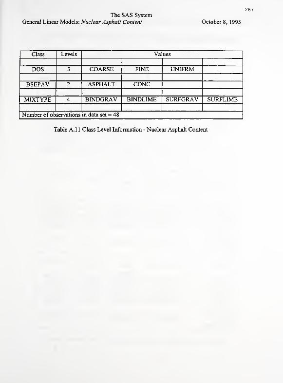
The SAS System
General Linear Models: Nuclear Asphalt Content
267
October 8, 1995
Class Levels Values
DOS 3 COARSE FINE UNIFRM
BSEPAV 2 ASPHALT CONC
MIXTYPE 4 BINDGRAV BINDLIME SURFGPvAV SURFLIME
Number of observations in data set = 48
Table A.l 1 Class Level Information - Nuclear Asphalt Content
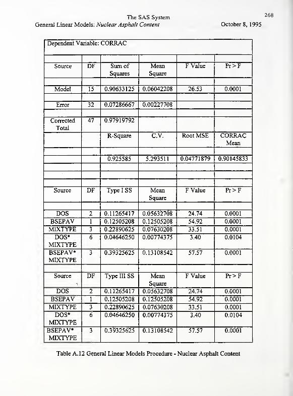
The SAS System
General Linear Models: Nuclear Asphalt Content
268
October 8, 1995
Dependent Variable: CORRAC
Source DF Sum of
Squares
MeanSquare
F Value Pr>F
Model 15 0.90633125 0.06042208 26.53 0.0001
Error 32 0.07286667 0.00227708
Corrected
Total
47 0.97919792
R-Square C.V. Root MSE CORRACMean
0.925585 5.293511 0.04771879 0.90145833
Source DF Type I SS MeanSquare
F Value Pr>F
DOS 2 0.11265417 0.05632708 24.74 0.0001
BSEPAV 1 0.12505208 0.12505208 54.92 0.0001
MIXTYPE 3 0.22890625 0.07630208 33.51 0.0001
DOS*MIXTYPE
6 0.04646250 0.00774375 3.40 0.0104
BSEPAV*MTXTYPE
3 0.39325625 0.13108542 57.57 0.0001
Source DF Type III SS MeanSquare
F Value Pr>F
DOS 2 0.11265417 0.05632708 24.74 0.0001
BSEPAV 1 0.12505208 0.12505208 54.92 0.0001
MIXTYPE 3 0.22890625 0.07630208 33.51 0.0001
DOS*MTXTYPE
6 0.04646250 0.00774375 3.40 0.0104
BSEPAV*MTXTYPE
3 0.39325625 0.13108542 57.57 0.0001
Table A. 12 General Linear Models Procedure - Nuclear Asphalt Content
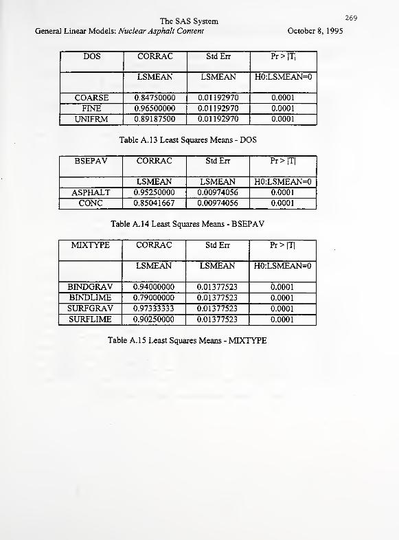
The SAS System
General Linear Models: Nuclear Asphalt Content
269
October 8, 1995
DOS CORRAC StdErr Pr>|T|
LSMEAN LSMEAN H0:LSMEAN=0
COARSE 0.84750000 0.01192970 0.0001
FINE 0.96500000 0.01192970 0.0001
UNIFRM 0.89187500 0.01192970 0.0001
Table A. 1 3 Least Squares Means - DOS
BSEPAV CORRAC StdErr Pr>|T|
LSMEAN LSMEAN H0:LSMEAN=0ASPHALT 0.95250000 0.00974056 0.0001
CONC 0.85041667 0.00974056 0.0001
Tat)le A. 14 Least Squares Means - BSEPAV
MIXTYPE CORRAC StdErr Pr > |T|
LSMEAN LSMEAN H0:LSMEAN=0
BINDGRAV 0.94000000 0.01377523 0.0001
BINDLIME 0.79000000 0.01377523 0.0001
SURFGRAV 0.97333333 0.01377523 0.0001
SURFLIME 0.90250000 0.01377523 0.0001
Table A. 15 Least Squares Means - MIXTYPE
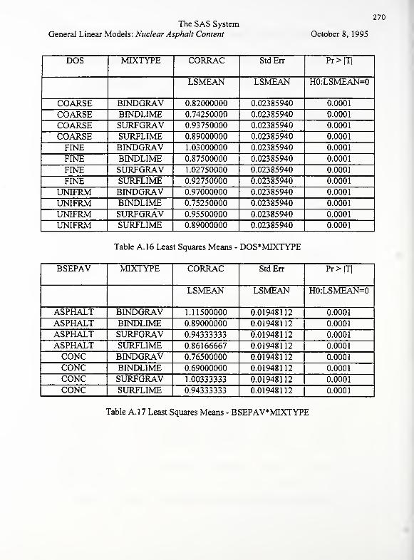
The SAS System
General Linear Models: Nuclear Asphalt Content
270
October 8, 1995
DOS MIXTYPE CORRAC StdErr Pr > |T|
LSMEAN LSMEAN H0:LSMEAN=0
COARSE BINDGRAV 0.82000000 0.02385940 0.0001
COARSE BINDLIME 0.74250000 0.02385940 0.0001
COARSE SURFGRAV 0.93750000 0.02385940 0.0001
COARSE SURFLIME 0.89000000 0.02385940 0.0001
FINE BINDGRAV 1.03000000 0.02385940 0.0001
FINE BINDLIME 0.87500000 0.02385940 0.0001
FINE SURFGRAV 1.02750000 0.02385940 0.0001
FINE SURFLIME 0.92750000 0.02385940 0.0001
UNIFRM BINDGRAV 0.97000000 0.02385940 0.0001
UNIFRM BINDLIME 0.75250000 0.02385940 0.0001
UNIFRM SURFGRAV 0.95500000 0.02385940 0.0001
UNIFRM SURFLIME 0.89000000 0.02385940 0.0001
Table A. 16 Least Squares Means - DOS*MIXTYPE
BSEPAV MIXTYPE CORRAC StdErr Pr > |T|
LSMEAN LSMEAN H0:LSMEAN=0
ASPHALT BINDGRAV 1.11500000 0.01948112 0.0001
ASPHALT BINDLIME 0.89000000 0.01948112 0.0001
ASPHALT SURFGRAV 0.94333333 0.01948112 0.0001
ASPHALT SURFLIME 0.86166667 0.01948112 0.0001
CONC BINDGRAV 0.76500000 0.01948112 0.0001
CONC BINDLIME 0.69000000 0.01948112 0.0001
CONC SURFGRAV 1.00333333 0.01948112 0.0001
CONC SURFLIME 0.94333333 0.01948112 0.0001
Table A. 17 Least Squares Means - BSEPAV*MIXTYPE
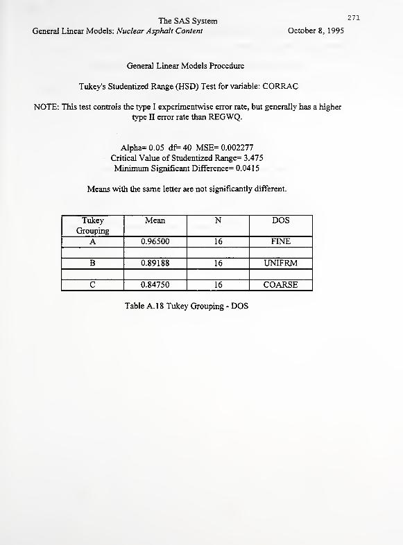
The SAS System
General Linear Models: Nuclear Asphalt Content
271
October 8, 1995
General Linear Models Procedure
Tukey's Studentized Range (HSD) Test for variable: CORRAC
NOTE: This test controls the type I experimentwise error rate, but generally has a higher
type II error rate than REGWQ.
Alpha= 0.05 df= 40 MSE= 0.002277
Critical Value of Studentized Range= 3.475
Minimum Significant Difference= 0.0415
Means with the same letter are not significantly different.
Tukey
Grouping
Mean N DOS
A 0.96500 16 FINE
B 0.89188 16 UNIFRM
C 0.84750 16 COARSE
Table A. 1 8 Tukey Grouping - DOS
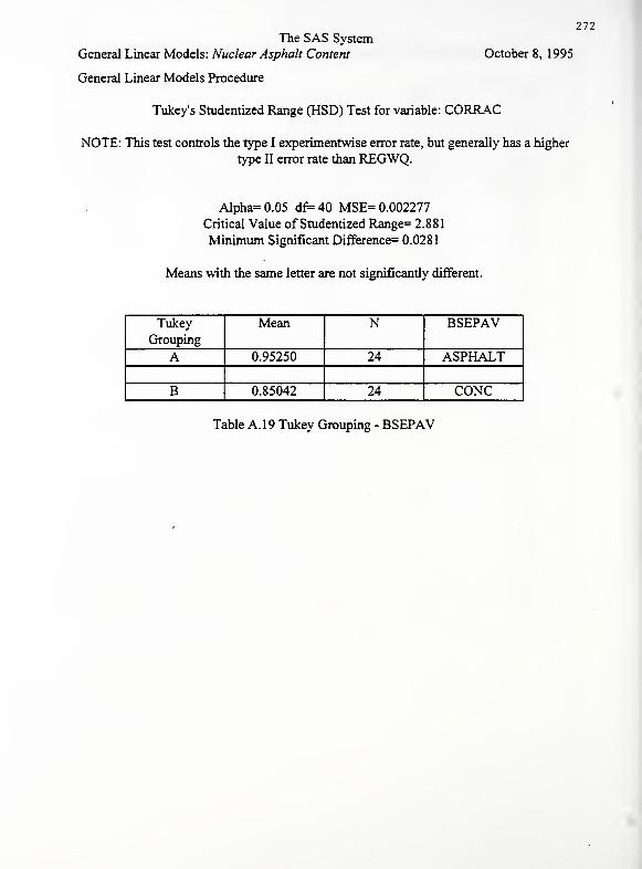
The SAS System
General Linear Models: Nuclear Asphalt Content
272
October 8, 1995
General Linear Models Procedure
Tukey's Studentized Range (HSD) Test for variable: CORRAC
NOTE: This test controls the type I experimentwise error rate, but generally has a higher
type II error rate than REGWQ.
Alpha=0.05 df=40 MSE= 0.002277
Critical Value of Studentized Range= 2.881
Minimum Significant Difference= 0.0281
Means with the same letter are not significantly different.
Tukey
Grouping
Mean N BSEPAV
A 0.95250 24 ASPHALT
B 0.85042 24 CONC
Table A. 19 Tukey Grouping - BSEPAV
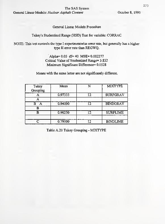
The SAS System
General Linear Models: Nuclear Asphalt Content
273
October 8, 1995
General Linear Models Procedure
Tukey's Studentized Range (HSD) Test for variable: CORRAC
NOTE: This test controls the type I experimentwise error rate, but generally has a higher
type II error rate than REGWQ.
Alpha= 0.05 df= 40 MSE= 0.002277
Critical Value of Studentized Range= 3.832
Minimum Significant Difference= 0.0528
Means with the same letter are not significantly different.
Tukey
Grouping
Mean N MIXTYPE
A 0.97333 12 SURFGRAVA
B A 0.94000 12 BINDGRAVBB 0.90250 12 SURFLIME
C 0.79000 12 BINDLIME
Table A.20 Tukey Grouping - MIXTYPE
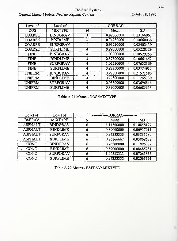
The SAS System
General Linear Models: Nuclear Asphalt Content
274
October 8, 1995
Level of Level of rORRACDOS MIXTYPE N Mean SD
COARSE BINDGRAV 4 0.82000000 0.23166067
COARSE BINDLIME 4 0.74250000 0.14660036
COARSE SURFGRAV 4 0.93750000 0.03403430
COARSE SURFLIME 4 0.89000000 0.05228129
FINE BINDGRAV 4 1.03000000 0.18529256
FINE BINDLIME 4 0.87500000 0.10661457
FINE SURFGRAV 4 1.02750000 0.07632169
FINE SURFLIME 4 0.92750000 0.03774917
UNIFRM BINDGRAV 4 0.97000000 0.21571586
UNIFRM BINDLIME 4 0.72500000 0.11265730
UNIFRM SURFGRAV 4 0.95500000 0.03696846
UNIFRM SURFLIME 4 0.89000000 0.06683313
Table A.21 Means - DOS*MIXTYPE
Level of Level of CORRAC
—
BSEPAV MIXTYPE N Mean SDASPHALT BINDGRAV 6 1.11500000 0.10858177
ASPHALT BINDLIME 6 0.89000000 0.06957011
ASPHALT SURFGRAV 6 0.94333333 0.03881580
ASPHALT SURFLIME 6 0.86166667 0.03868678
CONC BINDGRAV 6 0.76500000 0.11895377
CONC BINDLIME 6 0.69000000 0.08485281
CONC SURFGRAV 6 1.00333333 0.07061633
CONC SURFLIME 6 0.94333333 0.02065591
Table A.22 Means - BSEPAV*MLXTYPE
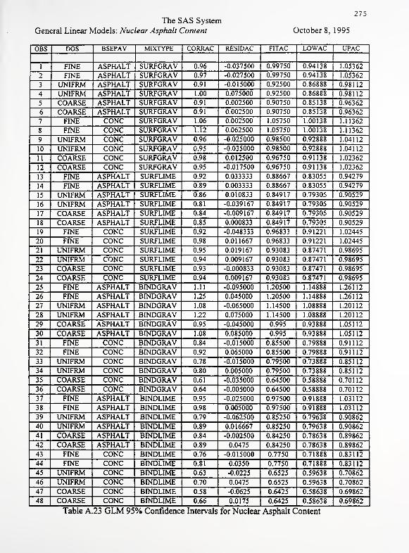
The SAS System
General Linear Models: Nuclear Asphalt Content
275
October 8, 1995
OBS DOS BSEPAV MIXTYPE CORRAC RESIDAC FITAC LOWAC UPAC
1 FINE ASPHALT SURFGRAV 0.96 -0.037500 0.99750 0.94138 1.05362
2 FINE ASPHALT SURFGRAV 0.97 -0.027500 0.99750 0.94138 1.05362
3 UNIFRM ASPHALT SURFGRAV 0.91 -0.015000 0.92500 0.86888 0.98112
4 UNIFRM ASPHALT SURFGRAV 1.00 0.075000 0.92500 0.86888 0.98112
5 COARSE ASPHALT SURFGRAV 0.91 0.002500 0.90750 0.85138 0.96362
6 COARSE ASPHALT SURFGRAV 0.91 0.002500 0.90750 0.85138 0.96362
7 FINE CONC SURFGRAV 1.06 0.002500 1.05750 1.00138 1.11362
8 FINE CONC SURFGRAV 1.12 0.062500 1.05750 1.00138 1.11362
9 UNIFRM CONC SURFGRAV 0.96 -0.025000 0.98500 0.92888 1.04112
10 UNIFRM CONC SURFGRAV 0.95 -0.035000 0.98500 0.92888 1.04112
11 COARSE CONC SURFGRAV 0.98 0.012500 0.96750 0.91138 1.02362
12 COARSE CONC SURFGRAV 0.95 -0.017500 0.96750 0.91138 1.02362
13 FINE ASPHALT SURFLIME 0.92 0.033333 0.88667 0.83055 0.94279
14 FINE ASPHALT SURFLIME 0.89 0.003333 0.88667 0.83055 0.94279
15 UNIFRM ASPHALT SURFLIME 0.86 0.010833 0.84917 0.79305 0.90529
16 UNIFRM ASPHALT SURFLIME 0.81 -0.039167 0.84917 0.79305 0.90529
17 COARSE ASPHALT SURFLIME 0.84 -0.009167 0.84917 0.79305 0.90529
18 COARSE ASPHALT SURFLIME 0.85 0.000833 0.84917 0.79305 0.90529
19 FINE CONC SURFLIME 0.92 -0.048333 0.96833 0.91221 1.02445
20 FINE CONC SURFLIME 0.98 0.011667 0.96833 0.91221 1.02445
21 UNIFRM CONC SURFLIME 0.95 0.019167 0.93083 0.87471 0.98695
22 UNIFRM CONC SURFLIME 0.94 0.009167 0.93083 0.87471 0.98695
23 COARSE CONC SURFLIME 0.93 -0.000833 0.93083 0.87471 0.98695
24 COARSE CONC SURFLIME 0.94 0.009167 0.93083 0.87471 0.98695
25 FINE ASPHALT BINDGRAV 1.11 -0.095000 1.20500 1.14888 1.26112
26 FINE ASPHALT BINDGRAV 125 0.045000 1.20500 1.14888 1.26112
27 UNIFRM ASPHALT BINDGRAV 1.08 -0.065000 1.14500 1.08888 1.20112
28 UNIFRM ASPHALT BINDGRAV 1.22 0.075000 1.14500 1.08888 1.20112
29 COARSE ASPHALT BINDGRAV 0.95 -0.045000 0.995 0.93888 1.05112
30 COARSE ASPHALT BINDGRAV 1.08 0.085000 0.995 0.93888 1.05112
31 FINE CONC BINDGRAV 0.84 -0.015000 0.85500 0.79888 0.91112
32 FINE CONC BINDGRAV 0.92 0.065000 0.85500 0.79888 0.91112
33 UNIFRM CONC BINDGRAV 0.78 -0.015000 0.79500 0.73888 0.85112
34 UNIFRM CONC BINDGRAV 0.80 0.005000 0.79500 0.73888 0.85112
35 COARSE CONC BINDGRAV 0.61 -0.035000 0.64500 0.58888 0.70112
36 COARSE CONC BINDGRAV 0.64 -0.005000 0.64500 0.58888 0.70112
37 FINE ASPHALT BINDLIME 0.95 -0.025000 0.97500 0.91888 1.03112
38 FINE ASPHALT BINDLIME 0.98 0.005000 0.97500 0.91888 1.03112
39 UNIFRM ASPHALT BINDLIME 0.79 -0.062500 0.85250 0.79638 0.90862
40 UNIFRM ASPHALT BINDLIME 0.89 0.016667 0.85250 0.79638 0.90862
41 COARSE ASPHALT BINDLIME 0.84 -0.002500 0.84250 0.78638 0.89862
42 COARSE ASPHALT BINDLIME 0.89 0.0475 0.84250 0.78638 0.89862
43 FINE CONC BINDLIME 0.76 -0.015000 0.7750 0.71888 0.83112
44 FINE CONC BINDLIME 0.81 0.0350 0.7750 0.71888 0.83112
45 UNIFRM CONC BINDLIME 0.63 -0.0225 0.6525 0.59638 0.70862
46 UNIFRM CONC BINDLIME 0.70 0.0475 0.6525 0.59638 0.70862
47 COARSE CONC BINDLIME 0.58 -0.0625 0.6425 0.58638 0.69862
48 COARSE CONC BINDLIME 0.66 0.0175 0.6425 0.58638 0.69862
Table A.23 GLM 95% Confidence Intervals for Nuclear Asphalt Content
276
APPENDIX DDiscriminant Analysis Output of Laboratory Nuclear Gauge Testing
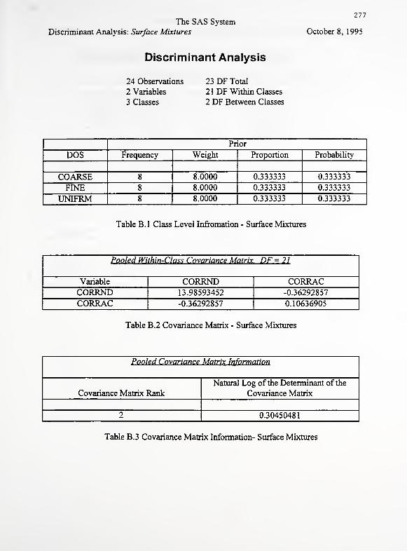
The SAS System
Discriminant Analysis: Surface Mixtures
277
October 8, 1995
Discriminant Analysis
24 Observations
2 Variables
3 Classes
23 DF Total
21 DF Within Classes
2 DF Between Classes
Prior
DOS Frequency Weight Proportion Probability
COARSE 8 8.0000 0.333333 0.333333
FINE 8 8.0000 0.333333 0.333333
UNIFRM 8 8.0000 0.333333 0.333333
Table B.l Class Level Infromation - Surface Mixtures
Pooled Within-Class Covariance Matrix. DF = 21
Variable CORRND CORRACCORRND 13.98593452 -0.36292857
CORRAC -0.36292857 0.10636905
Table B.2 Covariance Matrix - Surface Mixtures
Pooled Covariance Matrix Information
Covariance Matrix Rank
Natural Log of the Determinant of the
Covariance Matrix
2 0.30450481
Table B.3 Covariance Matrix Information- Surface Mixtures
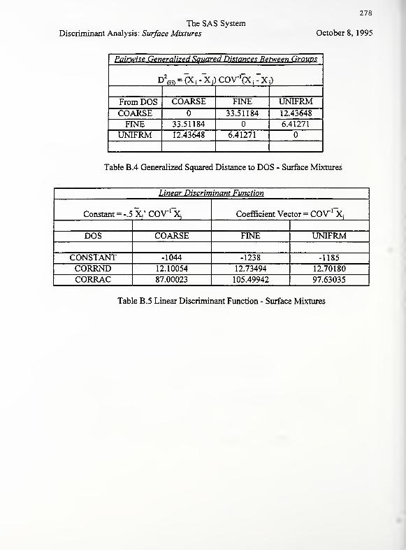
The SAS System
Discriminant Analysis: Surface Mixtures
278
October 8, 1995
Pairwise Generalized Squared Distances Between Groups
D^n-pCi-XOCOVfcj'x i)
From DOS COARSE FINE UNIFRMCOARSE 33.51184 12.43648
FINE 33.51184 6.41271
UNIFRM 12.43648 6.41271
Table B.4 Generalized Squared Distance to DOS - Surface Mixtures
Linear Discriminant Function
Constant = -.5 X,' COV*1"^Coefficient Vector = COV" 1 X
s
DOS COARSE FINE UNIFRM
CONSTANT -1044 -1238 -1185
CORRND 12.10054 12.73494 12.70180
CORRAC 87.00023 105.49942 97.63035
Table B.5 Linear Discriminant Function - Surface Mixtures
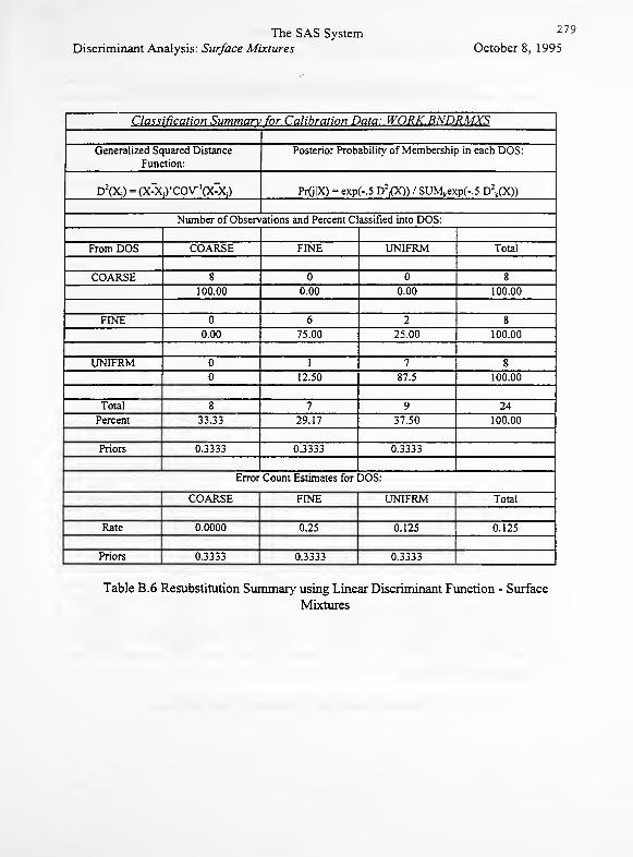
The SAS System
Discriminant Analysis: Surface Mixtures
279
October 8, 1995
Classification Summary for Calibration Data: WORK.BNDRMXS
Generalized Squared Distance
Function:
Posterior Probability of Membership in each DOS:
d2(Xj) = (xog'covr'cx'Xj) PrOIX) = exp(-.5 D 2
j(X)) / SUMkexp(-.5 D2
k(X))
Number of Observations and Percent Classified into DOS:
From DOS COARSE FINE UNIFRM Total
COARSE 8 8
100.00 0.00 0.00 100.00
FINE 6 2 8
0.00 75.00 25.00 100.00
UNIFRM 1 7 8
12.50 87.5 100.00
Total 8 7 9 24
Percent 33.33 29.17 37.50 100.00
Priors 0.3333 0.3333 0.3333
Error Count Estimates for DOS:
COARSE FINE UNIFRM Total
Rate 0.0000 0.25 0.125 0.125
Priors 0.3333 0.3333 0.3333
Table B.6 Resubstitution Summary using Linear Discriminant Function - Surface
Mixtures
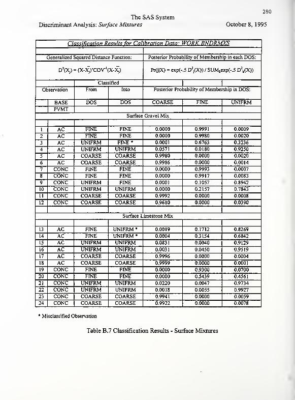
The SAS System
Discriminant Analysis: Surface Mixtures
280
October 8, 1995
Classification Results for Calibration Data: WORK.BNDRMXS
Generalized Squared Distance Function: Posterior Probability of Membership in each DOS:
D2(Xj) = (X-Xp'COV'(X-XJ) PrGiX) = exp(-.5 D2
j(X)) / SUMkexp(-.5 D2
t(X))
Classified1 1
Observation From Into Posterior Probability of Membership in DOS:
BASE DOS DOS COARSE FINE UNIFRMPVMT
Surface Gravel Mix
1 AC FINE FINE 0.0000 0.9991 0.0009
2 AC FINE FINE 0.0000 0.9980 0.0020
3 AC UNIFRM FINE* 0.0001 0.6763 0.3236
4 AC UNIFRM UNIFRM 0.0571 0.0180 0.9250
5 AC COARSE COARSE 0.9980 0.0000 0.0020
6 AC COARSE COARSE 0.9986 0.0000 0.0014
7 CONC FINE FINE 0.0000 0.9993 0.0007
8 CONC FINE FINE 0.0000 0.9917 0.0083
9 CONC UNIFRM FINE 0.0001 0.1057 0.8942
10 CONC UNIFRM UNIFRM 0.0000 0.2157 0.7843
11 CONC COARSE COARSE 0.9992 0.0000 0.0008
12 CONC COARSE COARSE 0.9610 0.0000 0.0390
Surface Limestone Mix
13 AC FINE UNIFRM* 0.0019 0.1712 0.8269
14 AC FINE UNIFRM* 0.0004 0.3154 0.6842
15 AC UNIFRM UNIFRM 0.0831 0.0040 0.9129
16 AC UNIFRM UNIFRM 0.0031 0.0450 0.9519
17 AC COARSE COARSE 0.9996 0.0000 0.0004
18 AC COARSE COARSE 0.9999 0.0000 0.0001
19 CONC FINE FINE 0.0000 0.9300 0.0700
20 CONC FINE FINE 0.0000 0.5439 0.4561
21 CONC UNIFRM UNIFRM 0.0220 0.0047 0.9734
22 CONC UNIFRM UNIFRM 0.0018 0.0055 0.9927
23 CONC COARSE COARSE 0.9941 0.0000 0.0059
24 CONC COARSE COARSE 0.9922 0.0000 0.0078
* Misclassified Observation
Table B.7 Classification Results - Surface Mixtures
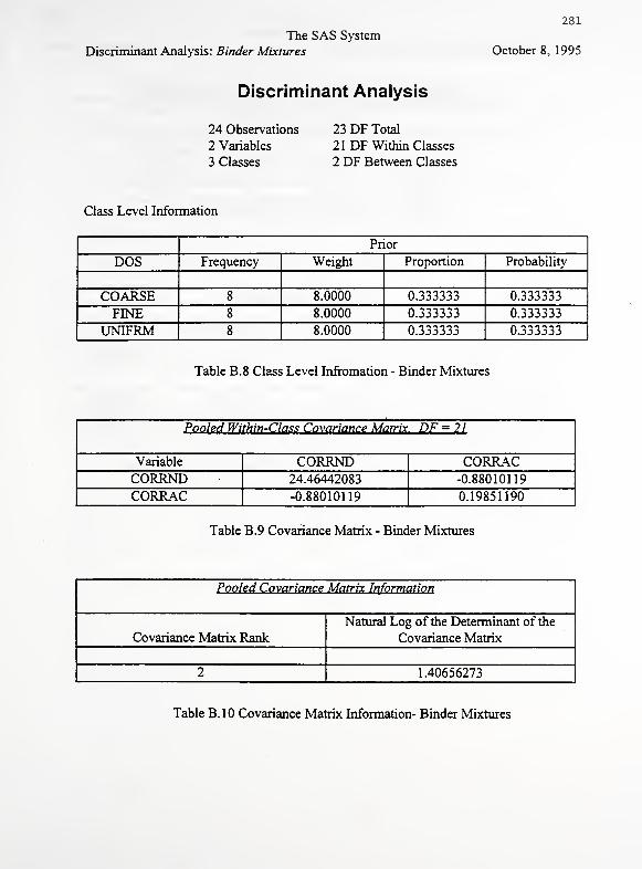
The SAS System
Discriminant Analysis: Binder Mixtures
281
October 8, 1995
Discriminant Analysis
24 Observations
2 Variables
3 Classes
23 DF Total
21 DF Within Classes
2 DF Between Classes
Class Level Information
Prior
DOS Frequency Weight Proportion Probability
COARSE 8 8.0000 0.333333 0.333333
FINE 8 8.0000 0.333333 0.333333
UNIFRM 8 8.0000 0.333333 0.333333
Table B.8 Class Level Infromation - Binder Mixtures
Pooled Within-Class Covariance Matrix. DF = 21
Variable CORRND CORRACCORRND 24.46442083 -0.88010119
CORRAC -0.88010119 0.19851190
Table B.9 Covariance Matrix - Binder Mixtures
Pooled Covariance Matrix Information
Covariance Matrix Rank
Natural Log of the Determinant of the
Covariance Matrix
2 1.40656273
Table B.10 Covariance Matrix Information- Binder Mixtures
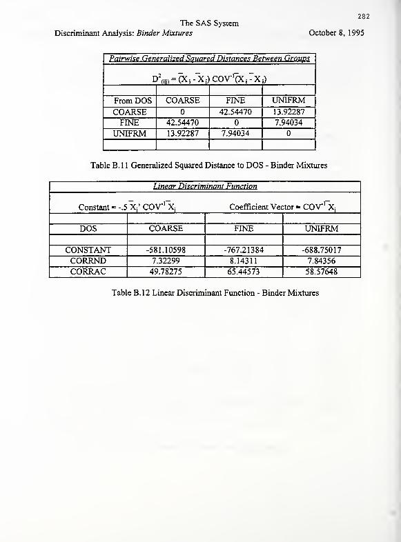
The SAS System
Discriminant Analysis: Binder Mixtures
282
October 8, 1995
Pairwise Generalized Squared Distances Between Groups
D^CXi-XOCOV'CXiOC i)
From DOS COARSE FINE UNIFRMCOARSE 42.54470 13.92287
FINE 42.54470 7.94034
UNIFRM 13.92287 7.94034
Table B.l 1 Generalized Squared Distance to DOS - Binder Mixtures
Linear Discriminant Function
Constant = -.5 X,' COV 1
X, Coefficient Vector = COV^X,
DOS COARSE FINE UNIFRM
CONSTANT -581.10598 -767.21384 -688.75017
CORRND 7.32299 8.14311 7.84356
CORRAC 49.78275 65.44573 58.57648
Table B.12 Linear Discriminant Function - Binder Mixtures
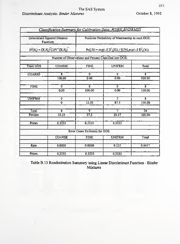
The SAS System
Discriminant Analysis: Binder Mixtures
283
October 8, 1995
Classification Summary for Calibration Data: WORK.BNDRMXS
Generalized Squared Distance
Function:
Posterior Probability of Membership in each DOS:
D2(Xi) = (x-Xjycov'pc-Xi)
-PrflIX) = exp(-.5 D 2
S
(X)) / SUM kexp(-.5 D2
k(X))
Number of Observations and Percent Classified into DOS:
From DOS COARSE FINE UNIFRM Total
COARSE S 8
100.00 0.00 0.00 100.00
FINE 8 8
0.00 100.00 0.00 100.00
UNIFRM 1 7 8
12.50 87.5 100.00
Total 8 9 7 24
Percent 33.33 37.5 29.17 100.00
Priors 0.3333 0.3333 0.3333
Error Count Estimates for DOS:
COARSE FINE UNIFRM Total
Rate 0.0000 0.0000 0.125 0.0417
Priors 0.3333 0.3333 0.3333
Table B.13 Resubstitution Summary using Linear Discriminant Function - Binder
Mixtures
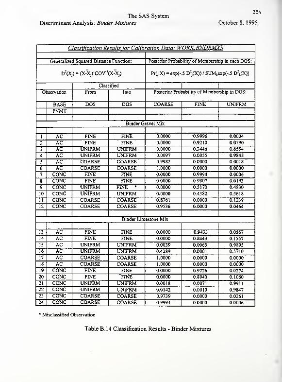
The SAS System
Discriminant Analysis: Binder Mixtures
284
October 8, 1995
Classification Results for Calibration Data: WORK.BNDRMXS
Generalized Squared Distance Function: Posterior Probability of Membership in each DOS:
D2(Xj) = (X-XjJ'COV'CX-'Xj) Ft(j|X) = exp(-.5 D2
j(X)) / SUMkexp(-.5 D2
k(X))
Classified1 1
Observation From Into Posterior Probability of Membership in DOS:
BASE DOS DOS COARSE FINE UNIFRMPVMT
Binder Gravel Mix
1 AC FINE FINE 0.0000 0.9996 0.0004
2 AC FINE FINE 0.0000 0.9210 0.0790
3 AC UNIFRM UNIFRM 0.0000 0.3446 0.6554
4 AC UNIFRM UNIFRM 0.0097 0.0055 0.9848
5 AC COARSE COARSE 0.9982 0.0000 0.0018
6 AC COARSE COARSE 1.0000 0.0000 0.0000
7 CONC FINE FINE 0.0000 0.9994 0.0006
8 CONC FINE FINE 0.0000 0.9807 0.0193
9 CONC UNIFRM FINE * 0.0000 0.5170 0.4830
10 CONC UNIFRM UNIFRM 0.0000 0.4382 0.5618
11 CONC COARSE COARSE 0.8761 0.0000 0.1239
12 CONC COARSE COARSE 0.9536 0.0000 0.0464
Binder Limestone Mix
13 AC FINE FINE 0.0000 0.9433 0.0567
14 AC FINE FINE 0.0000 0.8443 0.1557
15 AC UNIFRM UNIFRM 0.0039 0.0065 0.9895
16 AC UNIFRM UNIFRM 0.4289 0.0001 0.5710
17 AC COARSE COARSE 1.0000 0.0000 0.0000
18 AC COARSE COARSE 1.0000 0.0000 0.0000
19 CONC FINE FINE 0.0000 0.9726 0.0274
20 CONC FINE FINE 0.0000 0.8940 0.1060
21 CONC UNIFRM UNIFRM 0.0018 0.0071 0.9911
22 CONC UNIFRM UNIFRM 0.0142 0.0010 0.9847
23 CONC COARSE COARSE 0.9739 0.0000 0.0261
24 CONC COARSE COARSE 0.9994 0.0000 0.0006
Misclassified Observation
Table B.14 Classification Results - Binder Mixtures
285
APPENDIX EDiscriminant Analysis Output of Field Nuclear Gauge Testing
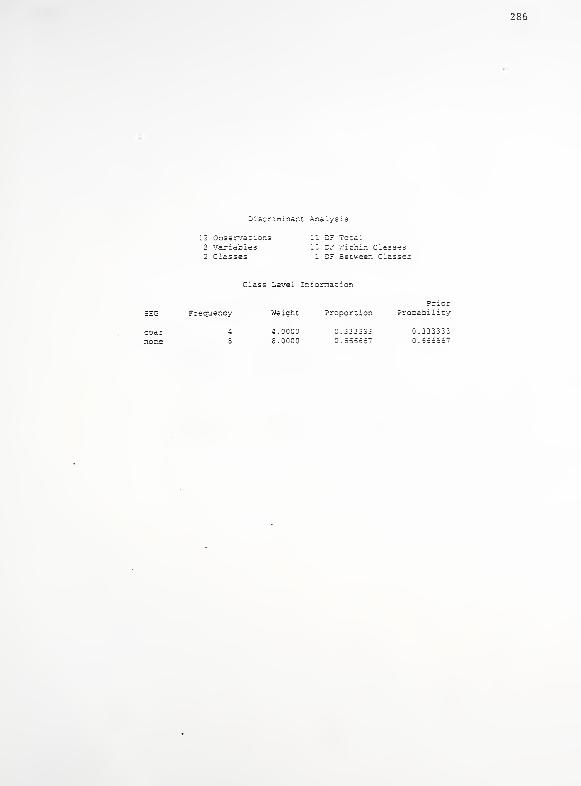
286
Discriminant Analysis
12 Observations 11 DF Total2 Variables 12 DF Vjithir. Classes2 Classes 1 DF Between Classes
Class Level Information
Prior
SEG Frequency Weight Proportion Prooability
coar 4 4.0000 C. 333332 0.333333
none S 8.00C0 0.666657 0.556567
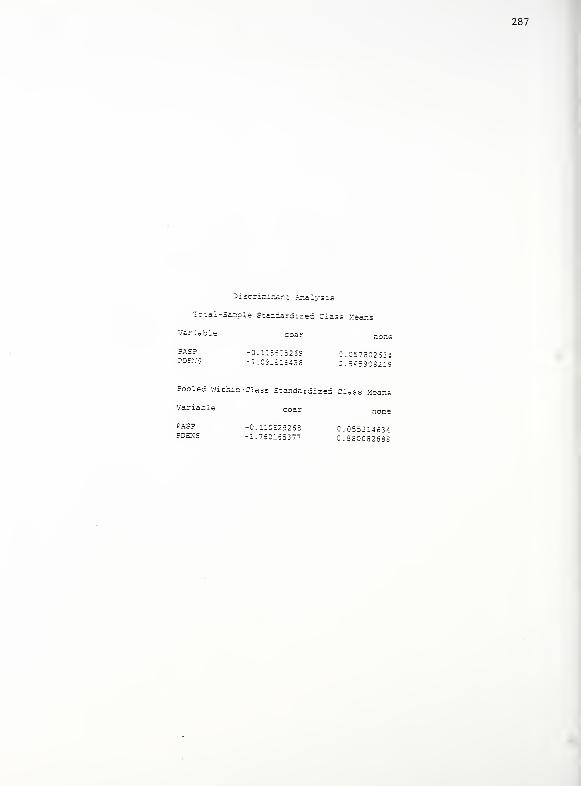
287
Qiscrininar.: Analysis
Tc-ai-SampIe Sta.-~azr6.izec. Class Means
Variable coar none
?AS? -0.1156:5259 1.057302524PDSNS -1.051=15438 0.545S08219
Pooled Wi thin-Class 3-andardized Class Means
Variable coar nong
PAS? -0.110529253 0.055314634PDENS -1.750155377 0.3S003268S

288
Pooled Covariancs Matrix ~-f omacior.
Covariar.cs Natural Log of Che Decern:.
Matrix Rank of the Covariar.ce Matrix
7.74352331
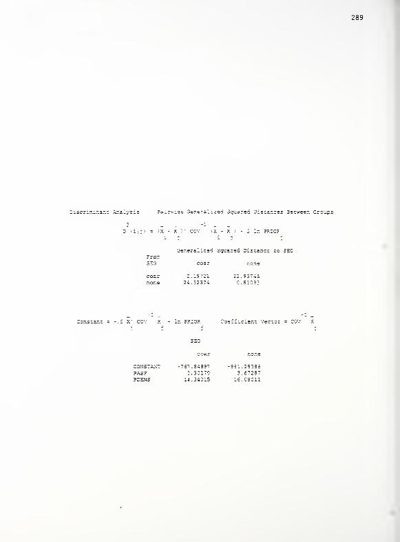
289
Discrir.ir.ar.; Analysis Pairwise Ger.era-ized Squared Distances Setweer. Groups
2 -1
D lijj) = (X - X i' COV (X - X )- 2 In PRIOR
Generalized Squared Distance to SEG
SEG coar none
coar 2.19722 22.93745none 24.32374 C.S1093
Constant = -.3 X' COV X - In PRIOR Coefficient Vector = COV
J ; J
coar none
CONSTANT -757.84897 -951.29386PAS? 3.30179 3.57287PDEN3 14.34015 16.08011
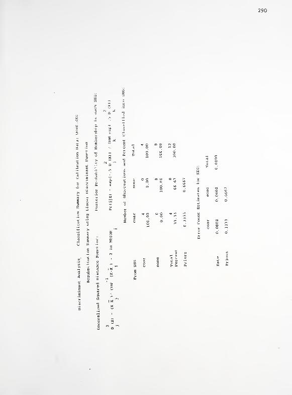
— ^r O
290
cc r- r*