CGS preconditioned with ILUT as a solver for circuit simulation
62
Nat.Lab. Unclassified Report 828/98 Date of issue: December 1998 CGS preconditioned with ILUT as a solver for circuit simulation Master Thesis Linda Lengowski UNCLASSIFIED NATLAB REPORT c Philips Electronics 1999
-
Upload
khangminh22 -
Category
Documents
-
view
1 -
download
0
Transcript of CGS preconditioned with ILUT as a solver for circuit simulation

Nat.Lab. Unclassified Report 828/98
Date of issue: December 1998
CGS preconditioned with ILUT as asolver for circuit simulationMaster Thesis
Linda Lengowski
UNCLASSIFIED NATLAB REPORTc Philips Electronics 1999

828/98 UNCLASSIFIED NATLAB REPORT
Authors' address data: [email protected]
c Philips Electronics N.V. 1999
All rights are reserved. Reproduction in whole or in part isprohibited without the written consent of the copyright owner.
ii c Philips Electronics N.V. 1999
UNCLASSIFIED NATLAB REPORT 828/98
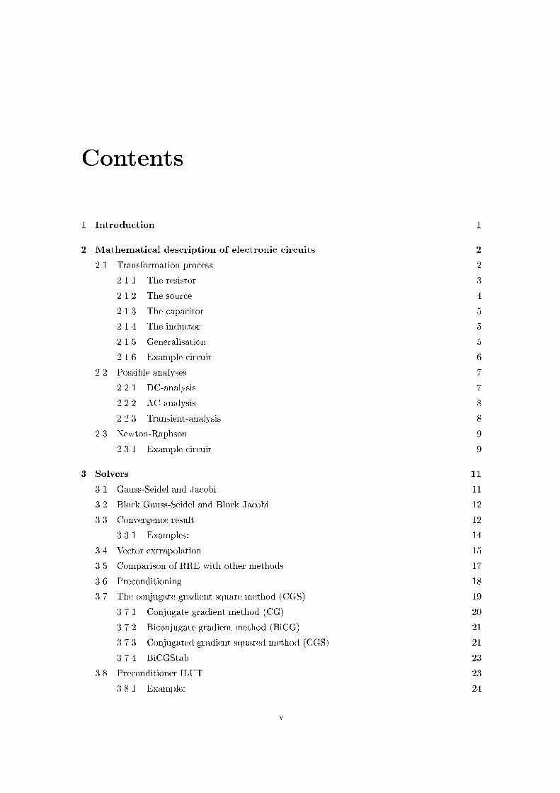
Unclassi�ed Report: 828/98
Title: CGS preconditioned with ILUT as a solver for circuit simulation
Master Thesis
Author(s): Linda Lengowski
Part of project:
Customer:
Keywords: Circuit simulation, BGS, CGS, ILUT
Abstract: In the design process of analogue circuits, lots of simulations are done
with circuit simulators to tune the behaviour of the circuit to meet its
requirements. Reducing the CPU-time needed for such a simulation is
a constant point of attention.
During these simulations, large sparse systems of equations need to be
solved. In this report, we concentrate on solving such intermediate lin-
ear systems and describe our experiments with several iterative meth-
ods. Options for improvement are discussed and the e�ect of precondi-
tioning is considered. The Conjugate Gradient Squared method (CGS),
preconditioned with an improved incomplete decomposition technique
(ILUT) showed to be the best.
The results are obtained for so called " at" circuits. A description is
given how the method can be implemented in Philips' analog circuit
simulator, Pstar, to simulate e�ciently hierarchical organized circuits.
This project was a co-operation between Philips Research Eindhoven
(Dept. ED&T/AS) and the Eindhoven Technical University.
It was executed at the Philips Nat.Lab. Eindhoven under supervision
of dr. E.J.W. ter Maten (Philips Electronic Design & Tools, Analogue
Simulation), dr. W.H.A. Schilders, (Philips Research, VLSI Design Au-
tomation and Test), dr. E.F. Kaasschieter (TUE) and prof. dr. R.M.M. Mattheij
(TUE).
Conclusions: See Chapter 6
c Philips Electronics N.V. 1999 iii

828/98 UNCLASSIFIED NATLAB REPORT
iv c Philips Electronics N.V. 1999
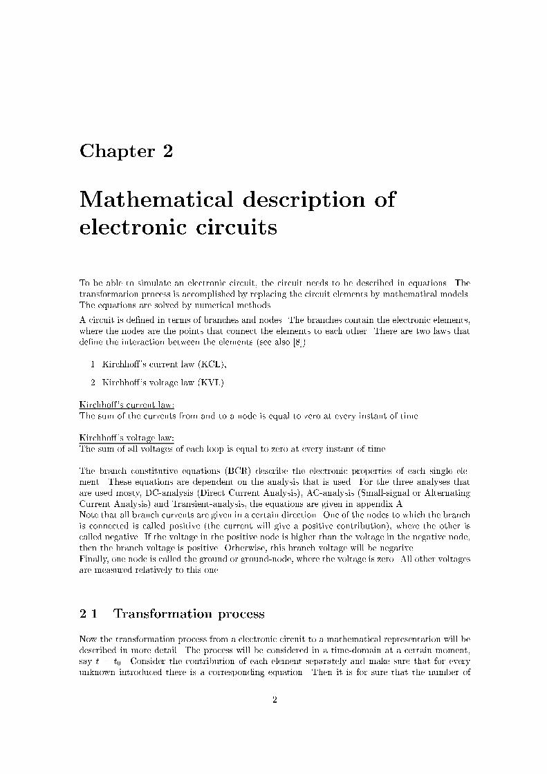
Contents
1 Introduction 1
2 Mathematical description of electronic circuits 2
2.1 Transformation process . . . . . . . . . . . . . . . . . . . . . . . . . . . . . . . . . 2
2.1.1 The resistor . . . . . . . . . . . . . . . . . . . . . . . . . . . . . . . . . . . . 3
2.1.2 The source . . . . . . . . . . . . . . . . . . . . . . . . . . . . . . . . . . . . 4
2.1.3 The capacitor . . . . . . . . . . . . . . . . . . . . . . . . . . . . . . . . . . . 5
2.1.4 The inductor . . . . . . . . . . . . . . . . . . . . . . . . . . . . . . . . . . . 5
2.1.5 Generalisation . . . . . . . . . . . . . . . . . . . . . . . . . . . . . . . . . . 5
2.1.6 Example circuit . . . . . . . . . . . . . . . . . . . . . . . . . . . . . . . . . . 6
2.2 Possible analyses . . . . . . . . . . . . . . . . . . . . . . . . . . . . . . . . . . . . . 7
2.2.1 DC-analysis . . . . . . . . . . . . . . . . . . . . . . . . . . . . . . . . . . . . 7
2.2.2 AC-analysis . . . . . . . . . . . . . . . . . . . . . . . . . . . . . . . . . . . . 8
2.2.3 Transient-analysis . . . . . . . . . . . . . . . . . . . . . . . . . . . . . . . . 8
2.3 Newton-Raphson . . . . . . . . . . . . . . . . . . . . . . . . . . . . . . . . . . . . . 9
2.3.1 Example circuit . . . . . . . . . . . . . . . . . . . . . . . . . . . . . . . . . . 9
3 Solvers 11
3.1 Gauss-Seidel and Jacobi . . . . . . . . . . . . . . . . . . . . . . . . . . . . . . . . . 11
3.2 Block Gauss-Seidel and Block Jacobi . . . . . . . . . . . . . . . . . . . . . . . . . . 12
3.3 Convergence result . . . . . . . . . . . . . . . . . . . . . . . . . . . . . . . . . . . . 12
3.3.1 Examples: . . . . . . . . . . . . . . . . . . . . . . . . . . . . . . . . . . . . . 14
3.4 Vector extrapolation . . . . . . . . . . . . . . . . . . . . . . . . . . . . . . . . . . . 15
3.5 Comparison of RRE with other methods . . . . . . . . . . . . . . . . . . . . . . . . 17
3.6 Preconditioning . . . . . . . . . . . . . . . . . . . . . . . . . . . . . . . . . . . . . . 18
3.7 The conjugate gradient square method (CGS) . . . . . . . . . . . . . . . . . . . . . 19
3.7.1 Conjugate gradient method (CG) . . . . . . . . . . . . . . . . . . . . . . . . 20
3.7.2 Biconjugate gradient method (BiCG) . . . . . . . . . . . . . . . . . . . . . 21
3.7.3 Conjugated gradient squared method (CGS) . . . . . . . . . . . . . . . . . 21
3.7.4 BiCGStab . . . . . . . . . . . . . . . . . . . . . . . . . . . . . . . . . . . . . 23
3.8 Preconditioner ILUT . . . . . . . . . . . . . . . . . . . . . . . . . . . . . . . . . . . 23
3.8.1 Example: . . . . . . . . . . . . . . . . . . . . . . . . . . . . . . . . . . . . . 24
v

828/98 UNCLASSIFIED NATLAB REPORT
4 Numerical Results 26
4.1 The test set of electronic circuits . . . . . . . . . . . . . . . . . . . . . . . . . . . . 26
4.2 Block Gauss-Seidel (BGS) . . . . . . . . . . . . . . . . . . . . . . . . . . . . . . . . 26
4.2.1 Variation of the coupling factor . . . . . . . . . . . . . . . . . . . . . . . . . 27
4.2.2 BGS in combination with RRE . . . . . . . . . . . . . . . . . . . . . . . . . 28
4.3 GMRES preconditioned with ILUT . . . . . . . . . . . . . . . . . . . . . . . . . . . 28
4.4 CGS preconditioned with ILUT . . . . . . . . . . . . . . . . . . . . . . . . . . . . . 30
4.4.1 Order of the variables . . . . . . . . . . . . . . . . . . . . . . . . . . . . . . 30
4.4.2 Eigenvalues . . . . . . . . . . . . . . . . . . . . . . . . . . . . . . . . . . . . 33
4.4.3 Comparison to comparable methods . . . . . . . . . . . . . . . . . . . . . . 34
5 A hierarchical solver 36
5.1 Hierarchical construction . . . . . . . . . . . . . . . . . . . . . . . . . . . . . . . . . 36
5.1.1 Example circuit . . . . . . . . . . . . . . . . . . . . . . . . . . . . . . . . . . 36
5.2 CGS in the hierarchy . . . . . . . . . . . . . . . . . . . . . . . . . . . . . . . . . . . 37
5.3 The hierarchical version of LU and ILUT decomposition . . . . . . . . . . . . . . . 38
5.4 The preconditioned CGS in the hierarchy . . . . . . . . . . . . . . . . . . . . . . . 40
6 Conclusions 42
A Branch equations 43
B Test circuits 44
B.1 Onebitadc . . . . . . . . . . . . . . . . . . . . . . . . . . . . . . . . . . . . . . . . . 44
B.2 Counter . . . . . . . . . . . . . . . . . . . . . . . . . . . . . . . . . . . . . . . . . . 45
B.3 Sram128 . . . . . . . . . . . . . . . . . . . . . . . . . . . . . . . . . . . . . . . . . . 46
B.4 dac5b right . . . . . . . . . . . . . . . . . . . . . . . . . . . . . . . . . . . . . . . . 47
B.5 ER 7899 . . . . . . . . . . . . . . . . . . . . . . . . . . . . . . . . . . . . . . . . . . 48
C Coupling factor and partitioning 49
C.1 Dynamic partitioning . . . . . . . . . . . . . . . . . . . . . . . . . . . . . . . . . . . 49
C.2 Adaptive coupling factor . . . . . . . . . . . . . . . . . . . . . . . . . . . . . . . . . 50
Bibliography 53
Distribution
vic Philips Electronics N.V. 1999

Chapter 1
Introduction
The electronic circuits that are created nowadays consist of extremely high numbers of elements.To study the characterictics of these circuits, they are simulated by a program like Pstar [12]. Withthis circuit simulation program it is possible to get information about the system that cannot befound by electronic measurements. During the simulation, large, often sparse systems of linearequations need to be solved.Within Pstar this is in most cases done by a UL-decomposition. Other options that are possible,are the usage of Block Gauss-Seidel (BGS [10, 11]). The goal of this project was to extend thestudies [10, 11, 14] by studying improvement options for these methods and to compare their per-formances with other recently developed iterative solvers.As a result, CGS, preconditioned with ILUT (Incomplete LU-decomposition with threshold), ap-peared to be the best from the point of view of CPU-performance. In the study, we restrictedourselves to linear systems within Transient-analysis.
This report is structured as follows:The �rst chapter is this introduction. The second chapter explains how an electronic circuit canbe described by a system of (non-linear) equations. Here also, the intermediate linear systems aredescribed as occuring in DC-analysis, AC-analysis and Transient-analysis. The third chapter givesthe necessary theoretical background for the iterative methods that are investigated. Chapter 4lists and comments the numerical results found by using the mathematical program MATLAB5.2.0 [7]. Chapter 5 gives an idea how the chosen method can be implemented within Pstar, to-gether with an explanation about the hierarchy of an electronic circuit. Finally, Chapter 6 givesconclusions that can be drawn from the experiments.
1
Chapter 2
Mathematical description of
electronic circuits
To be able to simulate an electronic circuit, the circuit needs to be described in equations. Thetransformation process is accomplished by replacing the circuit elements by mathematical models.The equations are solved by numerical methods.
A circuit is de�ned in terms of branches and nodes. The branches contain the electronic elements,where the nodes are the points that connect the elements to each other. There are two laws thatde�ne the interaction between the elements (see also [8]).
1. Kirchho�'s current law (KCL),
2. Kirchho�'s voltage law (KVL).
Kirchho�'s current law:The sum of the currents from and to a node is equal to zero at every instant of time.
Kirchho�'s voltage law:The sum of all voltages of each loop is equal to zero at every instant of time.
The branch constitutive equations (BCR) describe the electronic properties of each single ele-ment. These equations are dependent on the analysis that is used. For the three analyses thatare used mosty, DC-analysis (Direct Current Analysis), AC-analysis (Small-signal or AlternatingCurrent Analysis) and Transient-analysis, the equations are given in appendix A.Note that all branch currents are given in a certain direction. One of the nodes to which the branchis connected is called positive (the current will give a positive contribution), where the other iscalled negative. If the voltage in the positive node is higher than the voltage in the negative node,then the branch voltage is positive. Otherwise, this branch voltage will be negative.Finally, one node is called the ground or ground-node, where the voltage is zero. All other voltagesare measured relatively to this one.
2.1 Transformation process
Now the transformation process from a electronic circuit to a mathematical representation will bedescribed in more detail. The process will be considered in a time-domain at a certain moment,say t = t0. Consider the contribution of each element separately and make sure that for everyunknown introduced there is a corresponding equation. Then it is for sure that the number of
2

UNCLASSIFIED NATLAB REPORT 828/98
equations is equal to the number of unknowns.Suppose that two nodes, a and b, are connected by an electronic element (�g. 2.1).
Elementa b
Figure 2.1: Part of an electronic circuit
While only looking at the connection between two nodes, the element can be
! a resistor,
! a source,
! an inductor or
! a capacitor.
Within Pstar, there are two options both for a resistor and a source:
! the 'I-def'-resistor and the 'V-def'-resistor,
! the current source and the voltage source.
The di�erence between these two resistors is that through the 'I-def'-resistor, the current i[R],where R is the resistor, is explicitly known. This is in contrast to the 'V-def'-resistor, in whichcase the current i[R] is added as an unknown variable. Before looking at the di�erent elements, anotation will be introduced �rst.De�ne the nodes of the circuit as nk and the voltages corresponding to that node as V N [k]. TheKCL generates then the following equation for node nk:
V N [k] : 0 = : : : ; (2.1)
where the dots will be �lled by the contributions of the currents of the elements connected to nodek. In the next sections, n+ represents the positive node and n� represents the negative node.
2.1.1 The resistor
The resistor is given by the following symbol:
VN[-]VN[+] R
i[R]
V[R]
The 'I-def' resistor or linear resistor
Normally the resistor introduces three di�erent variables: the current i[R] and the voltages V N [+]and V N [�]. For this kind of resistor, the current is known and is given as i[R] = V [R]=R =(V N [+]� V N [�])=R.The following contributions are given to the system of equations. The KCL introduces:
V N [+] : 0 = : : :+ i[R] + : : :V N [�] : 0 = : : :� i[R] + : : :
c Philips Electronics N.V. 1999 3

828/98 UNCLASSIFIED NATLAB REPORT
The KVL introduces:
i[R] : 0 = V [R]� (V N [+]� V N [�])And �nally, the BCR introduces
0 = i[R]R� V [R]:
Now use the de�nition for i[R]. Both nodes can be given as an expression, only existing of nodevoltages. Therefore the current does not have to be introduced as an unknown variable. This�nally leads to the following contribution of the 'I-def'-resistor to the KCL equations:
V N [+] : 0 = : : :+ (V N [+]� V N [�])=R+ : : :V N [�] : 0 = : : :� (V N [+]� V N [�])=R+ : : :
The 'V-def' resistor
Because of the fact that the current is not explicitly known yet, the current must be introducedas an extra unknown. The resistor is de�ned by expressing V [R] as a function of the current i[R]:V [R] = f(i[R]). This leads to the following contribution to the system of equations:
V N [+] : 0 = : : :+ i[R] + : : :V N [�] : 0 = : : :� i[R] + : : :i[R] : 0 = V N [+]� V N [�]� f(i[R])
Note that this can be easily generalised to deal with implicit relations of the form g(i[R]; V [R]) = 0.As can easily be seen, the 'I-def' resistor is a special case of the 'V-def' resistor. The current i[R]is then given as a function of V [R].
2.1.2 The source
The current source
The current source is given by the following symbol:
VN[+] VN[-]
i[S]
V[S]
I(t)
Like for the 'I-def' resistor, the current i[S] is given, and therefore there are no new unknowsneeded to generate the equations. The contributions of this source are:
V N [+] : 0 = : : :+ I(t) + : : :V N [�] : 0 = : : :� I(t) + : : :
The voltage source
The voltage source is given by the following symbol:Analogously to the 'V-def' resistor, the current i[S] is not known. It does not depend explicitlyon the node voltages, but it is in uenced by the whole system. Thus the current i[S] needs to beadded as an extra unknown variable. This leads to the contributions of this source:
V N [+] : 0 = : : :+ i[S] + : : :V N [�] : 0 = : : :� i[S] + : : :i[S] : 0 = V (t)� (V N [+]� V N [�]):
4 c Philips Electronics N.V. 1999
UNCLASSIFIED NATLAB REPORT 828/98
VN[+] VN[-]
i[S]
V[S]
V(t)+ -
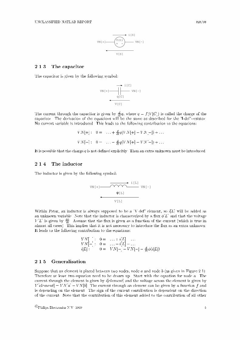
2.1.3 The capacitor
The capacitor is given by the following symbol:
VN[+] VN[-]
q[C]
V[C]
i[C]
The current through the capacitor is given by ddtq, where q = f(V [C]) is called the charge of the
capacitor. The derivation of the equations will be the same as described for the 'I-def'-resistor.No current variable is introduced. This leads to the following contribution to the equations:
V N [+] : 0 = : : :+ ddtq(V N [+]� V N [�]) + : : :
V N [�] : 0 = : : :� ddtq(V N [+]� V N [�]) + : : :
It is possible that the charge q is not de�ned explicitly. Then an extra unknown must be introduced.
2.1.4 The inductor
The inductor is given by the following symbol:
VN[+]
V[L]
VN[-]i[L]
φ[L]
Within Pstar, an inductor is always supposed to be a 'V-def' element, so i[L] will be added asan unknown variable. Note that the inductor is characterized by a ux �[L] and that the voltageV [L] is given by d�
dt. Assume that the ux is given as a function of the current (which is true in
almost all cases). This implies that it is not necessary to introduce the ux as an extra unknown.It leads to the following contribution to the equations:
V N [+] : 0 = : : :+ i[L] + : : :V N [�] : 0 = : : :� i[L] + : : :
i[L] : 0 = V N [+]� V N [�]� ddt�(i[L])
2.1.5 Generalisation
Suppose that an element is placed between two nodes, node a and node b (as given in Figure 2.1).Therefore at least two equation need to be drawn up. Start with the equation for node a. Thecurrent through the element is given by i[element] and the voltage across the element is given byV [element] = V N [a]� V N [b]. The current through an element can be given by a function f andis depending on the element. The sign of the current contribution is dependent on the directionof the current. Note that the contribution of this element added to the contribution of all other
c Philips Electronics N.V. 1999 5

828/98 UNCLASSIFIED NATLAB REPORT
elements connected to node a must be equal to zero.The same procedure can be used for node b. This way of creating equations for the branch currentsat each node, by using KCL, is called nodal analysis. Note that the system can formally be writtenas
i(v) +d
dtq(v) = 0; (2.2)
where i; v and q are "generalized"quantities. In some cases, the current through the elementneeds to be added as an extra unknown variable and therefore an additional equation need to bedrawed up. This is done by using KVL. The combined approach of creating the equations (withthese extra unknown variables) is called modi�ed nodal analysis.To transform a whole circuit to a system of equations, this procedure needs to be done for allelements in the circuit.
Remarks:
1. The additional unknowns i[R] and i[L] are used for convenience in order to deal with thenon-linear expressions.
2. Instead of using only currents as additional unknowns, �L and qC can be added as unknownvariables also. Combination of unknowns is another possibility.
3. If all contributions of all elements in a circuit are put together, then a system of �rst order,non-linear algebraic-di�erential equations arises.
2.1.6 Example circuit
In this section, an example circuit is considered to show the complete system of equations of acircuit instead of only elements. The circuit is shown in Figure 2.2.
1 2 3
R2
R1
C2
C1L1+
-V(t)
Figure 2.2: Example circuit
The transformation start with three KCL equations and three unknown variables V N [1], V N [2]and V N [3].
V N [1] : 0 = : : :V N [2] : 0 = : : :V N [3] : 0 = : : :
The contribution of the voltage source ('V-def') introduces an extra unknown i[S] and of coursean extra equation. This leads to:
V N [1] : 0 = i[S] + : : :V N [2] : 0 = : : :V N [3] : 0 = : : :i[S] : 0 = V (t)� V N [1]
6c Philips Electronics N.V. 1999

UNCLASSIFIED NATLAB REPORT 828/98
The contributions of both resistors lead to the following system (both linear resistors):
V N [1] : 0 = i[S]� (V N [1]� V N [2])=R1
V N [2] : 0 = (V N [1]� V N [2])=R1 + : : :V N [3] : 0 = �V N [3]=R2 + : : :i[S] : 0 = V (t)� V N [1]
The inductor introduces, with an explicit model of the ux, one extra variable i[L]. This leads to:
V N [1] : 0 = i[S]� (V N [1]� V N [2])=R1
V N [2] : 0 = (V N [1]� V N [2])=R1 � i[L] + : : :V N [3] : 0 = �V N [3]=R2 + : : :i[S] : 0 = V (t)� V N [1]i[L] : 0 = V N [2]� L1
ddti[L]
Finally, the in uence of the capacitors is given. Assume that the capacitor is modelled explicitly.This leads to:
V N [1] : 0 = i[S]� (V N [1]� V N [2])=R1
V N [2] : 0 = (V N [1]� V N [2])=R1 � i[L]� C1ddtV N [2]� C2
ddt(V N [3]� V N [2])
V N [3] : 0 = �V N [3]=R2 + C2ddt(V N [3]� V N [2])
i[S] : 0 = V (t)� V N [1]i[L] : 0 = V N [2]� L1
ddti[L])
2.2 Possible analyses
The three basic analyses: DC-analysis, AC-analysis and Transient-analysis are described in detailin the following subsections.
2.2.1 DC-analysis
DC-analysis of a circuit is the very basic analysis in a circuit simulation program and addresses thesteady-state solution. Hence all time-derivatives are zero and the time-dependent expressions areconstant. Hence the system simply is i(vDC) = 0. If the circuit is linear, then the circuit equationsfor DC-analysis form a system of linear equations. DC-analysis of a linear system needs only amethod to describe the circuit into equations and a linear solver to solve the system of equations.Modi�ed nodal analysis, de�ned as above, is the easiest method to transform the circuit in termsof equations. The system of these linear equations can be solved by, e.g., LU-decomposition.
Example circuit
Now consider the circuit as given in Figure 2.2. The system of equations is given above. Forthe DC-analysis, it holds that V (t) = VDC (constant), C1
ddtV N [k] = C2
ddtV N [k] = 0 and that
L1ddti[L]) = 0. If the above equations are rewritten with these data, then the following system
arises:0BBBBB@
�1R1
1R1
0 1 01R1
�1R1
0 0 �1
0 0 �1R2
0 0
1 0 0 0 00 �1 0 0 0
1CCCCCA
0BBB@
V N [1]V N [2]V N [3]i[S]i[L]
1CCCA =
0BBB@
000V
0
1CCCA
This linear system can be solved by LU-decomposition. The solution is V N [1] = V , V N [2] =V N [3] = 0 and i[S] = i[L] = V=R1.
c Philips Electronics N.V. 1999 7
828/98 UNCLASSIFIED NATLAB REPORT
2.2.2 AC-analysis
AC-analysis determines the perturbation of the solution of the circuit, due to small sinusoidalsources. AC means alterning current and applies to small input AC-sources. Another name issmall-signal analysis. This kind of analysis is a frequency-domain analysis and the equations arelinearised around the solution obtained by the DC-analysis. In comparison to DC-analysis, theequations for AC-analysis can be derived in nearly the same way. The only di�erence is that thecircuit equations are complex if AC-analysis is used. The equations that need to be solved inAC-analysis, can be found in the following way.Start again from:
i(v) +d
dtq(v) = 0:
Now de�ne v = vDC + x, where x = xACej!t and xAC is constant. Linearisation of this system
leads to:
i(vDC) +di
dv(vDC)x+
d
dt[q(vDC) +
dq
dv(vDC)x] = 0:
Note that i(vDC) = 0 (de�nition of vDC) and q(vDC) = constant and therefore ddt[q(vDC)] = 0.
Note that dqdv(vDC) is also time-independent. This will lead to the following equation:
di
dvx+
dq
dv
d
dtx = 0 ) (
di
dv+ j!
dq
dv)x = 0 8t ) (
di
dv+ j!
dq
dv)xAC = 0;
where ( didv
+ j! dqdv) is a complex matrix. AC-analysis has his own (extra) sine-wave sources for the
voltage- and current-sources. These sources are additional to the DC-sources (and may be assignedto other nodes than for the DC-sources).So, AC-analysis consists of
1. DC-analysis,
2. Compute all didv
and dqdv
in v = vDC ,
3. Solve the complex system of linear equations (in practice for a sweep of several frequences!).
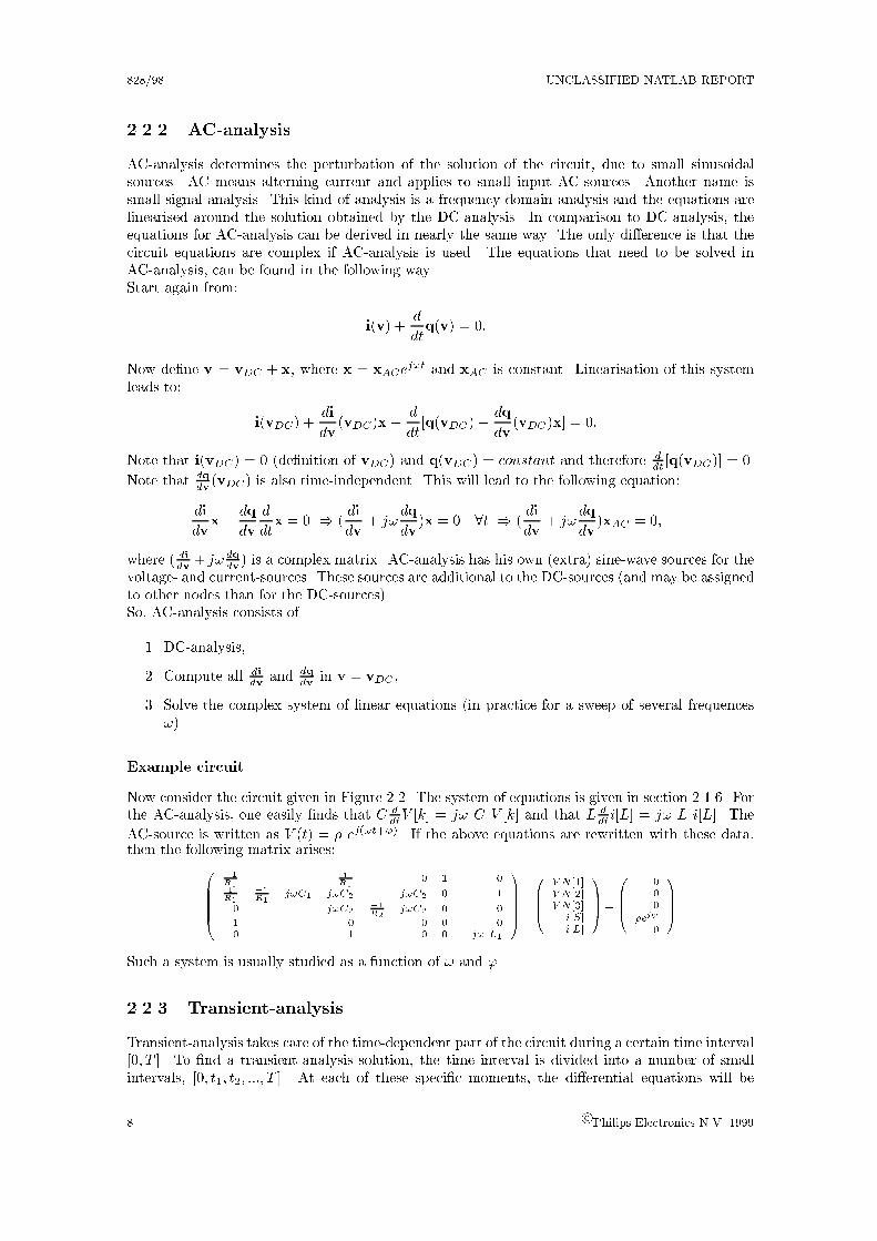
Example circuit
Now consider the circuit given in Figure 2.2. The system of equations is given in section 2.1.6. Forthe AC-analysis, one easily �nds that C d
dtV [k] = j! C V [k] and that L d
dti[L] = j! L i[L]. The
AC-source is written as V (t) = � ej(!t+'). If the above equations are rewritten with these data,then the following matrix arises:
0BBBBB@
�1R1
1R1
0 1 01R1
�1R1
� j!C1 + j!C2 �j!C2 0 �1
0 �j!C2�1R2
+ j!C2 0 0
1 0 0 0 00 �1 0 0 �j! L1
1CCCCCA
0BBB@
V N [1]V N [2]V N [3]i[S]i[L]
1CCCA =
0BBB@
000
�ej'
0
1CCCA
Such a system is usually studied as a function of ! and '.
2.2.3 Transient-analysis
Transient-analysis takes care of the time-dependent part of the circuit during a certain time interval[0; T ]. To �nd a transient-analysis solution, the time interval is divided into a number of smallintervals, [0; t1; t2; :::; T ]. At each of these speci�c moments, the di�erential equations will be
8c Philips Electronics N.V. 1999

UNCLASSIFIED NATLAB REPORT 828/98
transformed by a numerical integration algorithm into algebraic equations. This implies that asystem of non-linear algebraic equations needs to be solved. The solution at t = 0 is determinedby the DC-solution and the solution of the transient-analysis can then be found iteratively. Thisnumerical integration can be implicit as well as explicit. For circuit simulation, in general, implicitmethods, like the backward di�erential formula (BDF) methods, are preferred. Within, e.g., theEuler backward method (which is the BDF method of order 1), the term d
dtq(v) in (2.2) can be
replaced by
d
dtq(v) � 1
�t(q(vk)� q(vk�1)) ; (2.3)
where �t = tk � tk�1 is the time step. This leads to the following equation, to be solved for vk attime tk:
q(vk) = q(vk�1) + �t i(vk); (2.4)
where q(vk�1) is known at time tk. For accurate approximation, the time step needs to be chosensmall enough. When dealing with solutions that show an oscillatory behaviour, the trapezoidalrule is applied to be able to deal with the imaginary eigenvalues.
2.3 Newton-Raphson
Application of the modi�ed nodal analysis to a circuit and the usage of a suitable time integrationmethod (within Transient Analysis), will lead to a system of non-linear algebraic equations foreach discretisation point ti. These equations can generally be described as
F(x) = 0;
where x = xi is the vector of the unknown variables at moment ti (where x can be voltagesand currents). The Newton-Raphson method is often used in simulation programs because of itse�ciency. Newton-Raphson starts with an initial solution x0. The m-th iteration of the Newton-Raphson process then is
J(xm�1)xm = J(xm�1)xm�1 �F(xm�1): (2.5)
J(xm�1) = @F@x
is the Jacobian matrix of F, evaluated at xm�1, and m the iteration number of theNewton-Raphson proces. Equation 2.5, with A = J(xm�1) en B = Axm�1 � F(xm�1), will leadto
Axm = B: (2.6)
Note that the RHS of (2.5) can be determined very e�ciently by elementwise assembly of contri-butions to the matrix and to F. This system of equations is a linearised system of the equationsand can be solved by LU-decomposition. The iteration process continues until the values xk andxk+1 agree within some error tolerance.
Within Transient analysis, equation (2.4) describes the function F directly. Note that J(x) =1�t
dqdv(x)+ di
dv(x). A system with as coe�cient matrix such J(x) will be solved in Chapter 4, using
the methods described in Chapter 3.
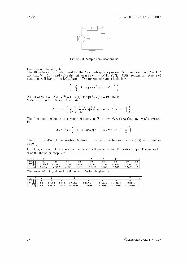
2.3.1 Example circuit
To explain the Newton-Raphson method a bit more, it will be applied to the system given in�gure 2.3. Instead of two linear resistors, one is replaced by a variable resistance. The currentthrough this resistance is described as i(v) = v+2v2+ v3, with v = V N [2]� 0 = V N [2]. This will
c Philips Electronics N.V. 1999 9
828/98 UNCLASSIFIED NATLAB REPORT
R1 2
i(v)
I[S]+
-V(t)
Figure 2.3: Simple non-linear circuit
lead to a non-linear system.The DC-solution will determined by the Newton-Raphson process. Suppose now that R = 1 and that V = 20 V and write the unknown as v = (V N [1]; V N [2]; i[S]). Solving this system ofequations will lead to the DC-solution. The functional matrix looks like
0@
1R
� 1R
1
� 1R
1R+ 1 + 4V N [2] + 3V N [2]2 0
1 0 0
1A
As initial solution take: v(0) = (V N [1]0; V N [2]0; i[S]0) = (20; 16; 4).Written in the form F(x) = 0 will give:
F(x) =
0@
�i[S] + V N [1]� V N [2]
�V N [1] + 2V N [2] + 2V N [2]2 + V N [2]3
V N [1]� 20
1A =
0@
000
1A :
The functional matrix to this system of equations F at x(m�1), with m the number of iterationsis:
J(x(m�1)
) =
0@
1 �1 �1
�1 2 + 4V N [2](m�1) + 3(V N [2]2)(m�1) 01 0 0
1A
The m-th iteration of the Newton-Raphson proces can then be described as (2.5) and thereforeas (2.6).
For the given example, the system of equation will converge after 8 iteration steps. The values forx at the iterations steps are
#iter 1 2 3 4 5 6 7 8 9V N [1] 20 20 20 20 20 20 20 20 20V N [2] 10.4604 6.7938 4.4109 2.9553 2.2260 2.0168 2.0001 2.0000 2I[S] 9.5396 13.2062 15.5891 17.0447 17.7740 17.9832 17.9999 18.0000 18
The error jvi � ~vj, where ~v is the exact solution, is given by
#iter 1 2 3 4 5 6 7 8 9V N [1] 0 0 0 0 0 0 0 0 0V N [2] 8.46 4.7938 2.4109 9.5532e-1 2.2598e-1 1.6752e-2 1.0182e-4 3.6362e-9 0I[S] 8.46 4.7938 2.4109 9.5532e-1 2.2598e-1 1.6752e-2 1.0182e-4 3.6362e-9 0
10 c Philips Electronics N.V. 1999

Chapter 3
Solvers
In this chapter we collect some mathematical background of several iterative methods to solve asystem of linear equations Ax = b. The given n � n�matrix A is called the coe�cient matrix,the vector x of length n is the vector of unknowns and the vector b of length n is called the right-hand side vector. We will consider (Block) Gauss-Seidel (Section 3.1- 3.3), vector extrapolation(Section 3.4- 3.5), CGS (Section 3.7). Numerical experiences will be postponed until the nextchapter. Special details of Gauss-Seidel when applied to a circuit from practice can be found in [6].Good general references are [13, 2, 22].
3.1 Gauss-Seidel and Jacobi
Let a nonsingular n� n-matrix A and a sparse system of linear equations
Ax = b (3.1)
be given. For large systems, direct methods are too expensive and therefore iterative methods areoften used. However, instead of �nding an exact solution of equation 3.1, iterative methods �ndapproximate solutions xk that should converge to the exact solution. An iterative method alwaysstarts with an initial vector x0 and generates a sequence of solutions. The advantage of basiciterative methods is that they can determine a next iterand very fast and they are not di�cult toimplement. On the other hand, a disadvantage is that they may converge slowly or may convergenot at all.The following standard decomposition of matrix A can be introduced:
A = D�E�F: (3.2)
Here D is the diagonal of A, �E is the strictly lower triangular part of A and �F is the strictlyupper triangular part of A. A standard assumption is that the diagonal entries of matrix A arenonzero, so aii 6= 0. Note that this may not be valid when dealing with circuit analysis (see thematrices given in the previous chapter).
The Gauss-Seidel method is given as follows:During the solution of one of the unknown variables at the k-th iteration step, the variables thathave already been solved at the same iteration level as the unknown vector can be used directly asan input signal. The other variables are used from the previous iteration. This method gives thefollowing iteration prescription for the i-th component:
aiix(k+1)i = �
Xj<i
aijx(k+1)j �
Xj>i
aijx(k)j + bj : (3.3)
11

828/98 UNCLASSIFIED NATLAB REPORT
In matrix form, with de�nitions as given above, this looks like
Dx(k+1) = Ex(k+1) +Fx(k) + b; (3.4)
or
(D�E)x(k+1) = Fx(k) + b: (3.5)
The Jacobi method is given as follows:During the solution of one of the unknown variables at the k-th iteration step, the solution at theprevious iteration of all other variables will be used as an input signal. This leads to the followingprescription per iteration for the i-th component:
aiix(k+1)i = �
Xj 6=i
aijx(k)j + bj : (3.6)
In matrix form, with de�nitions as given above, this looks like
Dx(k+1) = (E+F)x(k) + b: (3.7)
3.2 Block Gauss-Seidel and Block Jacobi
Block iterative methods are generalisations of basic iterative methods. Matrices arising fromdi�erential methods often have a natural block structure where Aii are square matrices. Theconcept of block iterative methods is updating blocks instead of components. The vectors xk andbk, belonging to the block Ak will then be subsets of the vectors x and b. Now the same splittingas used for basic iterative methods (A = D � E � F) will be used, where E is a strictly lowertriangular matrix, F is a strictly upper triangular matrix and D is the diagonal. It is easy togeneralise the Gauss-Seidel method de�ned as above.An iteration prescription for the i-th vector is:
Aiix(k+1)i = �
Xj<i
Aijx(k+1)j �
Xj>i
Aijx(k)j + bj : (3.8)
In matrix form, with de�nitions as given above:
(D�E)x(k+1) = Fx(k) + b: (3.9)
For every iteration step, N systems of equations of the form
Ajjz = y; j = 1; :::; N; (3.10)
need to be solved. Note that this o�ers a way to deal with a scalar 0 on the diagonal, since thiscan be incorporated into a non-singular diagonal block.These last equations can be solved by LU-decompositions. Similar remarks apply to block Jacobi.
3.3 Convergence result
Iterative methods are supposed to converge to the exact solution of the problem x = A�1b. Assaid before every method starts with an initial vector x0 and produces a sequence of solutions(xi)i=1;:::;n. If this sequence converges to the exact solution, then the method is called convergent.
The Gauss-Seidel method is of the form Mx(k+1) = Nxk + b, where M = D � E and N = F.For Jacobi holds that M = D and N = E + F. Now de�ne G = M�1N and f = M�1b, thenx(k+1) = Gx(k) + f . The iteration matrix is de�ned as
G =M�1(M�A) = I�M�1A:
12 c Philips Electronics N.V. 1999

UNCLASSIFIED NATLAB REPORT 828/98
An important measure used for convergence is the spectral radius � of the matrix G. The spectralradius of G is de�ned as �(G) := max1�i�n j�ij, where �i are the eigenvalues of G.
Theorem 1. Consider an iterative method of the form x(k+1) =Gx(k) + f .
1. This method is convergent if and only if �(G) < 1.
2. It is su�cient for the convergence of an iterative method that kGk < 1, where kGk is de�nedas kGk = maxx6=0
kGxk
kxkand k:k is a vectornorm.
Proof. The proof can be found in [20].
Another way to investigate whether an iterative method is convergent is to consider its diagonaldominance. Note that a matrix is called irreducible if there is no permutation matrix P such thatPAP T is block upper triangular, where a block upper triangular matrix is of the form:� � �
0 ��
.A matrix A is called
� weakly diagonally dominant if jaiij �P
j 6=i jaij j, i = 1; :::; n,
� strongly diagonally dominant if jaiij >P
j 6=i jaij j, i = 1; :::; n,
� irreducibly diagonally dominant if A is irreducible and jaiij �P
j 6=i jaij j, but for at least onei it holds that jaiij >
Pj 6=i jaij j, i = 1; :::; n:
Theorem 2. Let A be strongly diagonally dominant or irreducibly diagonally dominant. Then
0 < �(GGS) < �(GGJ ) < 1.Thus both Jacobi and Gauss-Seidel are convergent.
Proof. The proof of this theorem is given in [20].
Consider matrix A. This matrix is called an M -matrix if it satis�es the following properties:
1. aii > 0 for i = 1; : : : ; n,
2. aij � 0 for i 6= j and i; j = 1; : : : ; n,
3. A is nonsingular,
4. A�1 � 0.
One expects that BGS converges faster than GS. Indeed, for the class of M -matrices, Theorem 3con�rms that the number of iterations needed for convergence of BGS is less than the number ofiterations using GS. Although the number of computations per iteration is higher while using BGSthan while using GS, this disadvantage will, in general, not exceed the advantage of the numbersof iterations.
Theorem 3. Consider an M-matrix A. Then:
�(GBGJ) � �(GGJ);�(GBGS) � �(GGS) and�(GBGS) � �(GBGJ):
Proof. This proof is given in [4], Theorems 6:6:1, 6:6:2 and 6:6:3.
c Philips Electronics N.V. 1999 13

828/98 UNCLASSIFIED NATLAB REPORT
3.3.1 Examples:
A is not an M-matrix
It is not always true that BGS converges faster than GS. To show the opposite, Varga [21], p. 80,considered a simple counter example:
A =
0@ 5 2 2
2 5 32 3 5
1A ; b =
0@ 9
1010
1A ; (3.11)
which has exact solution x = (1; 1; 1))T . Using Gauss-Seidel and block Gauss-Seidel, the resultsare shown in Figure 3.3.1a.
0 5 10 15 20 25 30 35 4010
−16
10−14
10−12
10−10
10−8
10−6
10−4
10−2
100
102
Number of iterations
testjob
GSBGS
(a) The system of equations in (3.11)
0 5 10 15 20 25 30 35 40 4510
−18
10−16
10−14
10−12
10−10
10−8
10−6
10−4
10−2
100
Number of iterations
testjob
GSBGS
(b) The system of equations in (3.12)
Figure 3.1: BGS versus GS
The eigenvalues of the iteration matrix of GS are f0; 0:29+ 0:1i; 0:29� 0:1ig. The eigenvalues ofthe iteration matrix of BGS are f0; 0; 0:39g.The fact that the spectral radius of the iteration matrix of GS is smaller than the spectral radiusof BGS explains the fact that GS converges faster than BGS. (�GS = 0:29; �BGS = 0:37).Note that the matrix given in (3.11) is not a M -matrix, but the inverse of a M -matrix.
A is an M-matrix
Consider the system Ax = b with
A =
0BBBBBB@
14
�116
�116
�116
2164
�1164
�116
�1164
2164
1CCCCCCA; b =
0BBBB@
18
332
332
1CCCCA ; (3.12)
in which the M -matrix A is the inverse of the matrix used in (3.11). Again the solution isx = (1; 1; 1)T . Now BGS converges faster than GS, shown in �gure 3.3.1b. The eigenvalues of theiteration matrix of GS are f0; �0:06; 0:45g. The eigenvalues of the iteration matrix of BGS aref0; 0:39; 0g. The spectral radia are given by �GS = 0:45; �BGS = 0:39.
14 c Philips Electronics N.V. 1999

UNCLASSIFIED NATLAB REPORT 828/98
0 10 20 30 40 50 60 70 80 90 10010
−16
10−14
10−12
10−10
10−8
10−6
10−4
10−2
100
102
Number of iterations
JBJ
(a) BJ versus GJ
0 10 20 30 40 50 60 70 8010
−16
10−14
10−12
10−10
10−8
10−6
10−4
10−2
100
102
Number of iterations
BGSBJ
(b) BGS versus BJ
Figure 3.2: Convergence behaviour while using matrix (3.12)
Finally consider BJ versus J and BJ versus BGS. The results are given in respectively Figure 3.3.1aand Figure 3.3.1b. The corresponding spectral radia are �BJ = 0:63 and �J = 0:67.
3.4 Vector extrapolation
A method to reduce the number of computations and iterations is vector extrapolation. The scalarextrapolation will be explained �rst, because of the fact that vector extrapolation is based on scalarextrapolation.The best known method to accelerate the convergence of a given sequence of values x(0), x(1), x(2),: : : is probably Aitken's method (better known as the 42-method of Aitken). Assume that thesequence converges towards the solution x. This can be represented as:
x(k+1) � x = (x(k) � x):
To �nd values for and x, the following equations will be used:
x(k+1) � x = (x(k) � x); (3.13)
x(k+2) � x = (x(k+1) � x): (3.14)
For , substract (3.13) from (3.14). x can be found by substitution of in (3.13). This will leadto
=x(k+2) � x(k+1)
x(k+1) � x(k); x =
x(k)x(k+2) � (x(k+1))2
x(k+2) � 2x(k+1) + x(k)(3.15)
The expression for x can be written in a more simple way by using the di�erence operator4x(k) :=x(k+1) � x(k) and 42x(k) := x(k+2) � 2x(k+1) + x(k). It will then look like
x = x(k) � (4x(k))2
42x(k):
The next theorem con�rms that the sequence generated by Aitken's method will converge fasterthan the original sequence.
c Philips Electronics N.V. 1999 15

828/98 UNCLASSIFIED NATLAB REPORT
Theorem 4. Assume that the sequence x(0), x(1), x(2), : : : converges towards x such that
x(k+1) � x = k(x(k) � x); lim
k!1 k = ; j j < 1;
and that x(k) 6= x; 8k�0.If k is large enough, then the sequence x̂(k), x̂(k+1), : : : , found by Aitken's method and de�ned by
x̂(k) = x(k) � (4x(k))2
42x(k);
exists and then
limk!1
x̂(k) � ~x
x(k) � x= 0:
Ste�ensen's method is based on Aitken's method. It starts by using the initial scalar x(0). Thescalars x(1) and x(2) are found by the original method. Because a sequence of three iterands isfound, Aitken's method can be used. Iterate x(2) will be replaced by this result. Use the originalrecipe to �nd the iteratives x(3) and x(4). Then again a sequence of three iterands is found andagain Aitken's method can be used. This procedure will be repeated until a solution is found thatis close enough to the exact solution.
Vector extrapolation, described here below, is based on Ste�ensen's method, but instead of us-ing scalars, vectors are used.Assume that a linear iteration process (for example the Gauss-Seidel method) generates a sequencex(0), x(1), : : : of vectors. The initial vector will be de�ned by x(0). The iteration process can bedescribed in an n-dimensional space by:
x(k+1) = Hx(k) + b;
where H is an n� n matrix. Similarly to the scalar case, the linear convergence can be describedas:
x(k+1) � x = H(x(k) � x); k = 0; 1; : : : : (3.16)
Let x(0), : : : , x(m+1) be the �rst m + 2 vectors in the sequence. The �rst and second orderdi�erences can be described by vectors as follows:
u(k) =4x(k) = x(k+1) � x(k); k = 0; 1; : : : ;m� 1;
andv(k) = 42x(k) = x(k+2) � 2x(k+1) + x(k); k = 0; 1; : : : ;m� 1:
Furthermore, de�ne the n� k matrices
U(k) = [u(0)ju(1)j : : : ju(k�1)] (3.17)
and
V(k) = [v(0)jv(1)j : : : jv(k�1)]: (3.18)
Substraction of two equations of the form (3.16) leads to:
x(k+2) � x(k+1) =H(x(k+1) � x(k)) = Hu(k);
which can be used to rewrite the equation for v(k):
v(k) = (x(k+2) � x(k+1))� (x(k+1) � x(k)) = (H� I)u(k): (3.19)
16 c Philips Electronics N.V. 1999

UNCLASSIFIED NATLAB REPORT 828/98
In matrix notation, this will look like:
V(k) = (H� I)U(k):
Assume that V(n) is nonsingular. Then apply the full rank extrapolation (FRE) (rang(V(n)) =k = n). It is easy to see that (H� I)�1 = U(n)(V(n))�1 and therefore
~x = x(0) �U(n)(V(n))�1u(0): (3.20)
Another way to write this equation is to introduce a temporary variable y. The equations thatneed to be solved are then
V(n)y = �u(0); (3.21)
~x = x(0) +U(n)y: (3.22)
A more useful extrapolation method is the reduced rank extrapolation (RRE), where k < n. Es-pecially for large systems, RRE will be prefered above FRE.Because of the fact that the matrices U(k) and V(k) are not square anymore, instead of eq. (3.21),the following equation need be solved
(V(k))TV(k)y = �(V(k))Tu(0): (3.23)
Note that
(V(k))+ = ((V(k))TV(k))�1(V(k))T ; (3.24)
where (V(k))+ is called the pseudo inverse (or Moore-Penrose generalized inverse). Therefore
y = �(V(n))+u(0); (3.25)
If the equation is written in the same form as (3.20), it will look like
~x = x(0) �U(n)(V(n))+u(0); (3.26)
Now consider a special case. If r = 1, then the matrices U(k) and V(k) consist of one single columnand y, given in equation (3.25), is just a scalar. In fact, the vector extrapolation method collapses
to the well known SOR-method, where ! =�(v(0))Tu(0)(v(0))Tv(0)
= y.
Now equation (3.22) simply becomes
~x = x(0) + yu(0): (3.27)
The same way as Ste�ensen used Aitken's method a several times, vector extrapolation can be useda several times after each other too. To use this, there must be at least a triplet of iterates thatcan be used to make an extrapolation. The vector extrapolation can be used with any linearlyconvergent iterative method, for example BGS or GS. To make sure that vector extrapolationwill give good results, the number of the start iterations and the internal iterations need to bedetermined. These are dependent on the speci�c matrix (or problem).
3.5 Comparison of RRE with other methods
Vector extrapolation methods can be partitioned into two families, the polynomial and the epsilonmethods. RRE belongs to the family of the polynomial methods together with the minimal poly-nomial method (MPE). In [17] it is proved that if these methods are applied to a linearly generated
c Philips Electronics N.V. 1999 17

828/98 UNCLASSIFIED NATLAB REPORT
vector sequence, they are Krylov methods. Furthermore, Van der Sluis ( [18]) proved that RREis mathematically equivalent to GMRES. GMRES is a method that minimizes the residual normover all vectors within the Krylov subspace Km. A Krylov subspace is a subspace of the formKm(A;v) = spanfv; Av; A2v; : : : ; Am�1vg. More information about GMRES can be foundin [13].To be able to prove the equivalency, RRE will be written in a di�erent way.The system that needs to be solved is Ax = b and consider the following iteration process:
x(i+1) = (I�A)x(i) + b: (3.28)
The matrices U and V are given in equations (3.17) and (3.18) (the indices are not mentionedanymore). De�ne ~y(i) and ~x(i) as
~y(i) = argminy2Rikx(1) � x(0) +Vyk;~x(i) = x(0) +U~y(i);
where k:k represents the Euclidean norm and V = �AU.
Theorem 5. Suppose that x(0) is an approximate solution and that ~b is given as ~b = b�Ax(0).
Note that x(1) � x(0) = b �Ax(0) = ~b. Then it holds that RRE is mathematically equivalent to
GMRES.
Proof.
(~x(i))GMRES = x(0) + argminx2Kik~b�Axk
= x(0) +Uargminy2Rik~b�AUyk= x(0) +Uargminy2Rikx(1) � x(0) +Vyk= x(0) +U~yi = ~x(i) = (~x(i))RRE
where Ki = spanf~b;A~b; : : : ;Ai�1~bg.Now it follows that GMRES is equivalent to RRE.
Remark:In practice the system solved by 3.28 will be equivalent to the one, one is interested in. Forinstance, if one wants to solve a system A1x = b1, with A1 = D + L + U, with GS, thenA = (D + L)�1U + I = (D + L)�1A1 and b = (D + L)�1b1. The Krylov subspaces are de�nedusing A rather than using A1.
3.6 Preconditioning
When solving systems by iterative methods, preconditioning plays an important role. The con-vergence speed of an iterative solver depends on the spectral properties of the matrix. These canbe in uenced by preconditioning of the matrix. There are three possible ways to precondition amatrix. These options are
1. Split preconditioning
2. Right preconditioning
3. Left preconditioning
To explain these options a bit more, start with the linear system of equations
Ax = b: (3.29)
18 c Philips Electronics N.V. 1999

UNCLASSIFIED NATLAB REPORT 828/98
The preconditioning matrix K needs to approximate the matrix A in some way and therefore thenew coe�cient matrix K�1A will have better spectral conditions, but the system
K�1Ax = K�1b (3.30)
will give the same solution as the system (3.29).The preconditioning matrix can be split in K =K1K2. The above given preconditioning is knownas left preconditioning. Split preconditiong is given by K�1
1 AK�12 , and the last preconditioning
technique (right preconditioning) is given by AK�12 K�1
1 . So it holds that preconditioning is atechnique that transforms the system
Ax = b (3.31)
to the system
~A~x = ~b; (3.32)
which has the same solution, but will have better spectral conditions. Therefore, the iterativemethods is expected to converge faster for system 3.32 than for the system 3.31. If a method iscalled preconditioned, it means that the system to which the method will be used is preconditioned.
Theorem 5 can also be given for a left or right preconditioned GMRES and RRE. This leads tothe following theorem.
Theorem 6. Suppose that x0 is an approximate solution and that ~b is given by ~b = b�Ax0.
1. the left preconditioned RRE is mathematically equivalent to the left preconditioned GMRES
2. the right preconditioned RRE is mathematically equivalent to the right preconditioned GMRES
Proof. 1. The proof of the equivalence is almost the same as the proof of Theorem 5.(~x(i))GMRES = x(0) + argminx2Ki
kM�1(~b�Ax)k= x(0) +Uargminy2RikM�1(~b�AUy)k= x(0) +Uargminy2Rikx(1) � x(0) +Vyk= x(0) +U~yi = ~x(i) = (~x(i))RRE
where Ki is now Ki = spanfM�1~b;M�1AM�1~b; : : : ; (M�1A)i�1M�1~bg.
2. The proof of the equivalence is again almost the same:
(~x(i))GMRES = x(0) +M�1argminx2Kik~b�AM�1xk
= x(0) +M�1Uargminy2Rik~b�AM�1Uyk= x(0) +M�1Uargminy2Rikx(1) � x(0) +Vyk= x(0) +M�1U~yi = (~x(i))RRE
where Ki is now Ki = spanfM�1~b;M�1AM�1~b; : : : ; (M�1A)i�1M�1~bg.It can be seen that RRE needs to be right preconditioned to be equivalent to the right pre-conditioned GMRES.
3.7 The conjugate gradient square method (CGS)
The CGS method is derived from the BiCG method (for asymmetric matrices), which itselve isderived from CG (for symmetric matrices). The CGS method is mainly developed to avoid theuse of the transpose of the matrix A, which is used in BiCG, and to gain a faster convergencewith almost the same amount of work as BiCG. To make it a bit more clear where the method iscoming from, the methods CG and BiCG will be explained �rst.
c Philips Electronics N.V. 1999 19
828/98 UNCLASSIFIED NATLAB REPORT
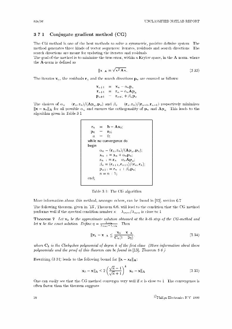
3.7.1 Conjugate gradient method (CG)
The CG method is one of the best methods to solve a symmetric, positive de�nite system. Themethod generates three kinds of vector sequences: iterates, residuals and search directions. Thesearch directions are meant for updating the iterates and residuals.The goal of the method is to minimize the true error, within a Krylov space, in the A-norm, wherethe A-norm is de�ned as
kxkA =pxTAx: (3.33)
The iterates xn, the residuals rn and the search directions pn are counted as follows:
xn+1 = xn + �npnrn+1 = rn � �nApnpn+1 = rn+1 + �npn
The choices of �n = (rn; rn)=(Apn;pn) and �n = (rn; rn)=(rn�1; rn�1) respectively minimizeskx � xnkA for all possible �n and ensures the orthogonality of pn and Apn. This leads to thealgorithm given in Table 3.1.
r0 = b�Ax0;p0 = r0;n = 0;
while no convergence dobegin
�n = (rn; rn)=(Apn;pn);xn+1 = xn + �npn;rn+1 = rn � �nApn;�n = (rn+1; rn+1)=(rn; rn);pn+1 = rn+1 + �npn;n = n+ 1;
end;
Table 3.1: The CG algorithm
More information about this method, amongst others, can be found in [13], section 6:7.
The following theorem, given in [13], Theorem 6:6, will lead to the condition that the CG-methodperforms well if the spectral condition number � = �max=�min is close to 1.
Theorem 7. Let xk be the approximate solution obtained at the k-th step of the CG-method and
let x be the exact solution. De�ne � = �min�max��min
. Then
kxk � xkA � kx0 � xkACk(1 + 2�)
; (3.34)
where Ck is the Chebychev polynomial of degree k of the �rst class. (More information about these
polynomials and the proof of this theorem can be found in [13], Theorem 6.6.)
Rewriting (3.34) leads to the following bound for kx� xkkA:
kxk � xkA � 2
�p�� 1p�+ 1
�kkx0 � xkA (3.35)
One can easily see that the CG-method converges very well if � is close to 1. The convergence isoften faster than the theorem suggests.
20 c Philips Electronics N.V. 1999

UNCLASSIFIED NATLAB REPORT 828/98
3.7.2 Biconjugate gradient method (BiCG)
The CG-method cannot be used for asymmetric matrices. One way to solve this problem is toapply CG to
Ax = b; and ATx� = b�;
in the form �0 A
AT 0
� �x�
x
�=
�b
b�
�;
where b� is arbitrary. The computation of the iterates stays the same. The computations of theresiduals and search directions are now:
rn+1 = rn � �nApnr�n+1 = r�n � �nA
Tp�n; r0 such that (r0; r�0) 6= 0
pn+1 = rn+1 + �npnp�n+1 = r�n+1 + �np
�n
The choices �n = (rn; r�n)=(Apn;p
�n) and �n = (rn+1; r
�n+1)=(rn; r
�n) ensure that the bi-orthogonality
relations ((ri; r�j ) = 0 and (Api;p
�j ) = 0 if i 6= j) are guarantueed. This leads to the algorithm
given in Table 3.2 (see also [13], Algorithm 7.3). Not much is known about the convergence be-
r0 = b�Ax0;Choose r�0 such that (r0; r
�0) 6= 0;
p0 = r0;p�0 = r�0;n = 0;
while no convergence dobegin
�n = (rn; r�n)=(Apn;p
�n);
xn+1 = xn + �npn;rn+1 = rn � �nApn;r�n+1 = r�n � �nA
Tp�n;�n = (rn+1; r
�n+1)=(rn; r
�n);
pn+1 = rn+1 + �npn�1;p�n+1 = r�n+1 + �np
�n�1;
n = n+ 1;end;
Table 3.2: The BiCG algorithm
haviour of BiCG. If ATA is positive de�nite, Theorem 3.34 can be applied with �'s being thesquare roots of the eigenvalues of ATA (i.e. � is a singular value of A). For symmetric, positivede�nite matrices A, BiCG gives the same result as CG, but needs twice as much costs per iterationas CG.
3.7.3 Conjugated gradient squared method (CGS)
The residuals vectors of BiCG can be written as rj = P (A)r0 and ~rj = P (AT )~r0, implying that�n = (P 2(A)r0; r
�0)=(Apn; r
�0) and � = (rn+1; r
�n+1)=(rn; r
�n). Indeed r
0j can be found, which plays
the same role as rj and ~rj and satis�es r0j = P 2(A)r0.
c Philips Electronics N.V. 1999 21

828/98 UNCLASSIFIED NATLAB REPORT
On this idea, the CGS-method is based. More detailed information can be found in [19].The major advantage of this method, when compared to BiCG, is that the use of AT is not longerneccessary. Furthermore, it holds that CGS converges often twice at fast as BiCG. A disadvantagecan be that the convergence behaviour can be very irregular. The CGS algorithm is given inTable 3.3, with initial vector x0 (see also for instance [2], Figure 2.9).
r0 = b�Ax0; r�0 such that (Ap0; r
�0) 6= 0
p0 = r0; u0 = r0n = 0;
while no convergence dobegin
�n = (rn; r�0)=(Apn; r
�0);
qn = un � �nApnxn+1 = xn + �n(un + qn);rn+1 = rn � �nA(un + qn);�n = (rn+1; r
�0)=(rn; r
�0);
un+1 = rn+1 + �nqn;pn+1 = un+1 + �n(qn + �npn);n = n+ 1;
end;
Table 3.3: The CGS algorithm
As before, it can be expected that preconditioning of the matrix will improve the convergence ofthe CGS-algorithm. De�ne PL as the matrix for left preconditioning and PR as the matrix forright preconditioning. Then the preconditioned system will look like:
~A~x = ~b;
where ~A = PLAPR, PR~x = x and ~b = PLb. Choose the matrices PL and PR in such a way thatthey create a matrix ~A which has better spectral properties than A. The product PLPR oftenrepresents an approximation of the inverse of A. If this preconditioning is used within CGS, thealgorithm is given in Table 3.4:
The amount of work S for this algorithm can be given in ops as:
S = SPL + SA +#iter(7N + 2+ 2(SA + SPL + SPR));
where SA, SPL and SPR represent respectively the amount of work to compute Ax, PLx and PRx
and N is the number of the variables. The amount of work for a sparse matrix is much less thanthe amount of work for a full matrix. A multiplication of a matrix and a vector costs for a fullmatrix N2 and for a sparse matrix only nz(A), where nz is the number of non-zeros of the matrixA. The circuit matrices are often very sparse and then holds nz(A) = O(N). This will lead to amuch cheaper CGS iteration step.Note that there are di�erent options for PL and PR. If the matrix will be preconditioned with anincomplete LU -decomposition, then there are the following options:
PL = L�1; PR = U�1;PL = I; PR = U�1L�1 andPL = U�1L�1; PR = I:
Finally something about the convergence properties of CGS. Although the CGS method does notneed a symmetric positive de�nite (SPD) matrix, the convergence behavour will be close to the
22 c Philips Electronics N.V. 1999

UNCLASSIFIED NATLAB REPORT 828/98
r0 = PL(b�Ax0);p0 = r0; u0 = r0
n = 0;while no convergence dobegin
vn = PLAPRpn;�n = (rn; r
�0)=(vn; r
�0);
qn = un � �nvnvn = �nPR(un + qn);xn+1 = xn + vn);rn+1 = rn �PLAvn;�n = (rn+1; r
�0)=(rn; r
�0);
un+1 = rn+1 + �nqn;pn+1 = un+1 + �n(qn + �npn);n = n+ 1;
end;
Table 3.4: The preconditioned CGS algorithm
SPD case if the matrix does not deviate too much from being positive de�nite. How much thematrix may di�er is not known, but if the method converges twice as fast as the BiCG method,one will understand that the convergence properties are almost equal to those of CG. Therefore,Theorem (3.35) can also be used for CGS.
3.7.4 BiCGStab
Finally, the BiCGStab method will be mentioned. In this method, the residual is generated, insteadof squaring the BiCG-polynomial (as done in CGS), as follows:
rj = ~Pj(A)P (A)r0; (3.36)
where ~Pj is a polynomial of degree j and ~Pj(0) = 1. A possible ~Pj(A) could be
~Pj(A) = (1� !1A)(1� !2A) : : : (1� !iA); (3.37)
with ! suitable constants.The BiCGStab can be seen as a product of BiCG and GMRES. The algorithm can be found in [2],Figure 2.10. The method was developed to smooth the irregular convergence behaviour of CGS.From the ideas of this method, the solver BiCGStab(l) is developed, as a product of BICG andGMRES(l) (which is the restarted GMRES after l iterations). This one is invented because evenBiCGStab sometimes causes stagnation or even break-downs. This is likely to happen if the matrixA is real and has complex eigenvalues with an imaginary part that is large when compared to thereal part. More details, and the algorithm, can e.g. be found in [14].
3.8 Preconditioner ILUT
Consider a general matrix A. A general incomplete LU-factorization (ILU) computes a sparselower triangular matrix L and a sparse upper triangular matrix U where instead of A = LU, itholds that A = LU +R, where R is the residual matrix. Some ILU-factorizations are based onthe structure of the matrix A and therefore make no use of the numerical values of the matrix.These methods only drop elements if there are non-zeros elements on places where matrix A was
c Philips Electronics N.V. 1999 23

828/98 UNCLASSIFIED NATLAB REPORT
empty. In other words, if the structure of the decomposed matrix di�ers from the structure of thematrix A itselves.A method that considers the numerical values of A is ILUT. There are two dropping rules withinthe ILUT-algorithm. If an element satis�es these dropping rules, it will be replaced by zero. Firstconsider the algorithm.
for i = 2; :::; n dofor k = 1; : : : ; i� 1 and aik 6= 0 do
lik = aik=akkApply dropping rule 1.for j = k + 1; : : : ; n do
if lik 6= 0aij = aij � likukj
endend
endApply dropping rule 2.uij = aij for j = i; : : : ; n
end
Table 3.5: The ILUT algorithm
The �rst dropping rule replaces the element lik, given by lik = aik=akk, by zero if it is smallerthan the relative drop-tolerance. The relative drop-tolerance �� is de�ned as �� = �kai�k, where� is the given drop-tolerance and kai�k is the Euclidean norm of row i. It is easy to see that thedropping rule is a relative criterion.
The second dropping rule reduces the number of elements in a row of the upper triangular matrix.The elements in the row that are smaller than the relative drop tolerance �� are replaced by zero.Note that the diagonal elements of U are always kept, although they might be smaller than therelative drop tolerance. Note that the second dropping rule is only applied to U .
3.8.1 Example:
To show the di�erence between LU and ILUT, a small example is given. For both options, thematrices U and L are given for all decomposition steps. Note that within the matrices U and Lformed by ILUT, the dropping rules are applied with tolerance � = 10�4.Note that the matrix is a �ctituous matrix and does not represent a practical electric circuit.Consider matrix A:
A =
0@
1 9:977e � 3 �1:225e� 4�9:621e � 3 2:882e+ 2 �1:293e� 4�1:293e � 3 �3:839e � 4 1:597e + 1
1A
First consider the standard LU-decomposition. After the �rst decomposition step, the matrices Land U will look like:
U =
0@
1 9:977e � 03 �1:225e � 040 2:882e+ 02 �1:305e � 040 3:710e � 04 1:597e+ 01
1A ; L =
0@
1 0 0�9:621e � 03 1 0�1:293e � 03 0 1
1A
24 c Philips Electronics N.V. 1999

UNCLASSIFIED NATLAB REPORT 828/98
After the second and last decomposition step, the matrices look like:
U =
0@
1 9:977e � 03 �1:225e� 040 2:882e + 02 �1:305e� 040 0 1:597e + 01
1A ; L =
0@
1 0 0�9:621e � 03 1 0�1:293e � 03 �1:287e� 06 1
1A
Now consider ILUT. The vector containing the relative droptolerances is �� = [1e � 04; 2:882e�02; 1:597e� 03]. After the �rst decomposition, the matrices look like:
U =
0@
1 9:977e� 03 �1:225e � 040 2:882e + 02 00 3:710e� 04 1:597e + 01
1A ; L =
0@
1 0 00 1 00 0 1
1A
After the second and last decomposition step, the matrices look like:
U =
0@
1 9:977e� 03 �1:225e � 040 2:882e + 02 00 0 1:597e + 01
1A ; L =
0@
1 0 00 1 00 0 1
1A
The residual matrix R = A� LU is given by
R =
0@
0 0 0�9:621e � 03 0 �1:293e � 04�1:293e � 03 �3:839e � 04 0
1A
Note that making an LU -decomposition in this case costs 11 ops, where ILUT costs only 3 ops,where the only operations that are counted are the multiplication and the division. One can easilysee that the �ll-in made by ILUT is much less than the �ll-in made by LU.
c Philips Electronics N.V. 1999 25

Chapter 4
Numerical Results
Transient analysis of electronic circuits is usually done by applying a backward di�erential formula(BDF) methods for time-integration. Each time step requires the solution of a non-linear system ofequations. We will assume that such a system is solved iteratively by Newton-Raphson's method.Then each new iterand is found by solving a linear system of equations. For details see Chapter 2.For solving such a linear system, the methods described in Chapter 3 will be applied. The presentchapter presents the numerical experiences with these methods for a limited number of electroniccircuits. The circuits are of di�erent sizes. The jobs that have been investigated are, with thenumber of the unknown variables written between brackets: onebitadc (58), counter (96), sram128(2624), dac5b (2477) and er7899 (2612). The study is done by using MATLAB 5.1 [7], using" at" matrices (i.e. no hierarchical datastructure was used). Note that all results presented hererepresent only one moment of time.
4.1 The test set of electronic circuits
The circuits used for this research are not especially created, but are circuits used in practice. Thesystems of equations come from a certain Newton-Raphson step within Pstar. The circuits in thisset show several characteristics. For the investigation, it is important to know how many elementsintroduce current variables and associated voltage equations. For all the above circuits, only thevoltage sources will give current variables and equations. Later on it will be shown that it is alsoimportant to know whether voltage sources are grounded or not.Finally, the number of elements of the circuit and a bit of the electronic background (the meaningof the circuit) will be given. These descriptions of the circuits used can be found in Appendix B.In the past some of these circuits have also been used in the research described in [11].
4.2 Block Gauss-Seidel (BGS)
To be able to use BGS, the matrix which represents the functional matrix of the Newton iterationneeds to be partitioned in blocks. The main idea of partitioning is to split the circuit into 'subcir-cuits' that are weakly coupled. The 'subcircuits' themselves exist of tightly coupled variables.Consider the iterative solver BGS where the assembly of the blocks is based on the followingcoupling criterion
jaij j > �jaiij _ jajij > �jajj j; (4.1)
where � is called the coupling factor and 0 � � � 1. If � = 0 then all variables are stronglycoupled. If � = 1 then all variables are weakly coupled. After applying this coupling criterion, the
26
UNCLASSIFIED NATLAB REPORT 828/98
strongly coupled pairs need to be placed in blocks. If two couples both contain the same variable,then they are placed in the same block.The number of strongly coupled variables will increase if � increases. This means that the numberof iterations needed for convergence will decrease if the coupling factor decreases. On the otherhand, the amount of work for each block will increase. The best solution is to �nd a compromisesomewhere in between. More details about this coupling and partioning criterion can be found inAppendix C .The linear system Ax = b will be solved iteratively up to a certain accuracy of the residual:
kAx� bkkbk < 10�5: (4.2)
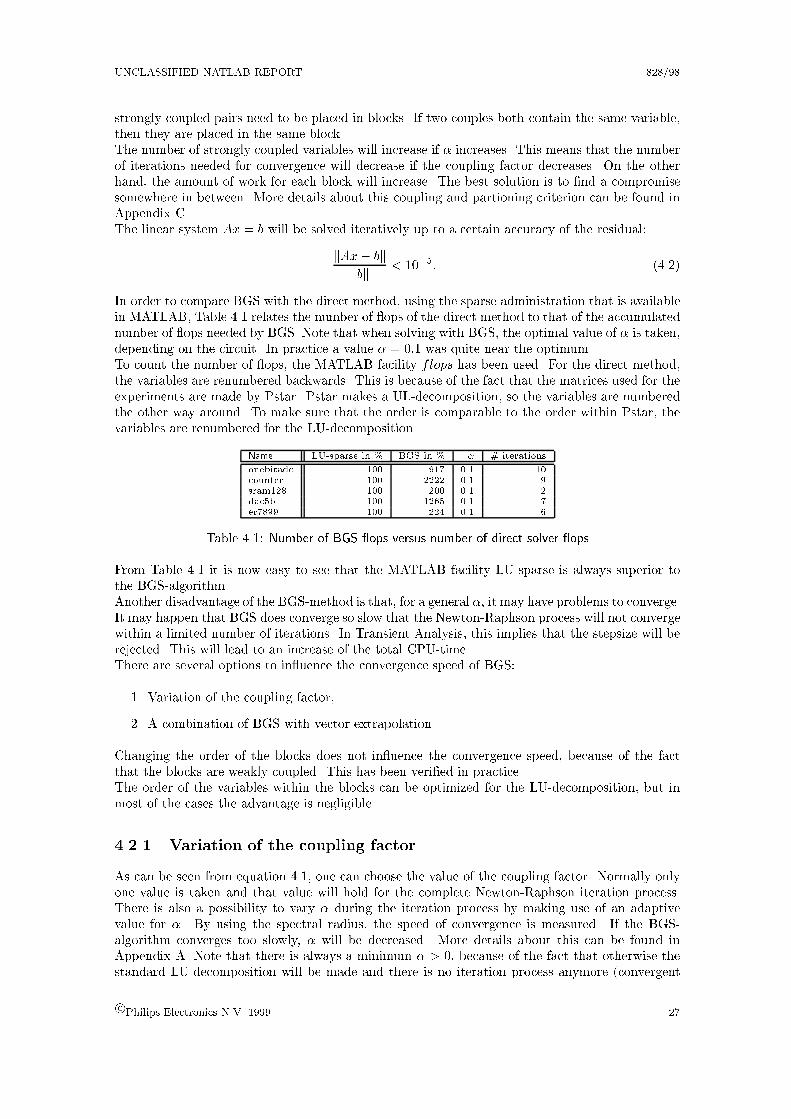
In order to compare BGS with the direct method, using the sparse administration that is availablein MATLAB, Table 4.1 relates the number of ops of the direct method to that of the accumulatednumber of ops needed by BGS. Note that when solving with BGS, the optimal value of � is taken,depending on the circuit. In practice a value � = 0:1 was quite near the optimum.To count the number of ops, the MATLAB facility flops has been used. For the direct method,the variables are renumbered backwards. This is because of the fact that the matrices used for theexperiments are made by Pstar. Pstar makes a UL-decomposition, so the variables are numberedthe other way around. To make sure that the order is comparable to the order within Pstar, thevariables are renumbered for the LU-decomposition.
Name LU-sparse in % BGS in % � # iterations
onebitadc 100 917 0.1 10counter 100 2222 0.1 9sram128 100 200 0.1 2dac5b 100 1265 0.1 7er7899 100 224 0.1 6
Table 4.1: Number of BGS ops versus number of direct solver ops
From Table 4.1 it is now easy to see that the MATLAB facility LU-sparse is always superior tothe BGS-algorithm.Another disadvantage of the BGS-method is that, for a general �, it may have problems to converge.It may happen that BGS does converge so slow that the Newton-Raphson process will not convergewithin a limited number of iterations. In Transient Analysis, this implies that the stepsize will berejected. This will lead to an increase of the total CPU-time.There are several options to in uence the convergence speed of BGS:
1. Variation of the coupling factor,
2. A combination of BGS with vector extrapolation.
Changing the order of the blocks does not in uence the convergence speed, because of the factthat the blocks are weakly coupled. This has been veri�ed in practice.The order of the variables within the blocks can be optimized for the LU-decomposition, but inmost of the cases the advantage is negligible.
4.2.1 Variation of the coupling factor
As can be seen from equation 4.1, one can choose the value of the coupling factor. Normally onlyone value is taken and that value will hold for the complete Newton-Raphson iteration process.There is also a possibility to vary � during the iteration process by making use of an adaptivevalue for �. By using the spectral radius, the speed of convergence is measured. If the BGS-algorithm converges too slowly, � will be decreased. More details about this can be found inAppendix A. Note that there is always a minimum � > 0, because of the fact that otherwise thestandard LU-decomposition will be made and there is no iteration process anymore (convergent
c Philips Electronics N.V. 1999 27

828/98 UNCLASSIFIED NATLAB REPORT
in 1 step). In practice, however, it appears that if there is a time step where BGS converges verybadly (� = 0:99), variation of the coupling factor is not much of a help. One will obtain lessiterations, however the total process will not be much faster in ops. This is the reason why onecannot expect this method to really improve the BGS process. New results are not presented herebecause of the fact that in Table 4.1 the most optimal � with respect to ops was chosen.
4.2.2 BGS in combination with RRE
If a system converges linearly, then it is possible to speed up this convergence with vector extrap-olation. For the problems where BGS converges very badly, it decreases the number of iterationsenormously. On the other hand, if BGS converges quite well, RRE will not give much advantage.In most of the cases it uses even more ops than BGS for the same accuracy of the residual. A hugedisadvantage is that the optimal number of iterands after which RRE will be applied (the "basis"of RRE), strongly depends on the problem and on the speci�c moment in the Newton-Raphsonprocess. Furthermore, a wrong choice of the number of these basic iterands can turn out that themethod does not improve the convergence speed of BGS.Because of the fact that no default number of basic iterands can be given, it is not a good optionto use in Pstar. The result of RRE with BGS is given in Figure 4.1. As can be seen, Figure 4.1arepresents a case where BGS converges very badly. RRE(5) gives an enormous decrease of thenumber of iterands (where RRE(k) means that the k-th iterant is replaced by the extrapolant.This extrapolant is the initial solution for the new serie of iterants). This �gure shows also anoption (RRE(3)) where the number of basic iterands is chosen too small. It is easy to see thatthe vector extrapolation gives a very bad result. In Figure 4.1b a moment where BGS convergesquite good is given. One can see that RRE(4) does not improve much the performance of BGS(although it is not shown in the �gure, RRE(5) does not improve the performance of BGS either).
4.3 GMRES preconditioned with ILUT
Because of the equivalence of RRE with GMRES (given in section 3.5), this method is the nextthat is looked after. Because of the fact that GMRES is quite expensive for the matrices producedby a circuit, due to ill-conditioned matrices, preconditioning is desirable (this holds also for RRE).The most common preconditioner is ILU(0), but this one only makes use of the structure of matrixA instead of the values. The preconditioning technique ILUT as presented in Chapter 3, makesuse of the values of the matrix and only replaces elements by zero if they are smaller than a certaintolerance. Because of this, preconditioning with ILUT is better than with ILU(0). This leadsto a faster convergence (less iterations for the same residual). That is why this preconditioningtechnique is chosen. The results of the GMRES algorithm preconditioned with ILUT, with droptolerance=10�4, are given in Table 4.2, again compared with the direct solver. The terminationcriterion that is used is
kAx� bkkbk < 10�5 (4.3)
Name LU sparse in % GMRES in % # iterations
onebitadc 100 106 3counter 100 144 2sram128 100 176 3dac5b 100 86 2er7899 100 141 2
Table 4.2: Number of GMRES ops versus number of direct solver ops
If Table 4.2 is compared with Table 4.1, one can easily deduce that the number of ops neededwhile using GMRES is less than the number of ops needed while using BGS. Another advantage of
28 c Philips Electronics N.V. 1999

UNCLASSIFIED NATLAB REPORT 828/98
0 5 10 15 20 25 30 35 40 45 5010
−16
10−14
10−12
10−10
10−8
10−6
10−4
10−2
100
102
Number of iterations
Res
idua
l
BGSBGS−RRE(3)BGS−RRE(5)
(a) Variation of the number of start iterations
0 2 4 6 8 10 12 1410
−18
10−16
10−14
10−12
10−10
10−8
10−6
10−4
10−2
100
Number of iterations
Res
idua
l
BGS BGS with RRE(4)
(b) In uence of RRE if BGS converges well
Figure 4.1: BGS with vector extrapolation
c Philips Electronics N.V. 1999 29

828/98 UNCLASSIFIED NATLAB REPORT
GMRES above BGS is that it always converges quite fast (for an n�nmatrix the maximum numberof iterations is n, but in the cases that are considered here, the maximum number of iterationsneeded for a residual less than 10�5 is only 3. Note that this is extremely small for such an iterativesolver). On the other hand, in most of the cases, it clearly is not faster than the direct sparse LU-decomposition (note that the optimal value for the drop-tolerance is chosen). To �nd a method thatmight be able to be faster than the LU-decomposition, four other iterative solvers for asymmetricmatrices are investigated. These methods are the conjugated gradient square method (CGS), thebiconjugate gradient algorithm (BiCG), the biconjugate gradient stabilized (BiCGStab) and thequasi-minimum residual algorithm (QMR). Note that all methods use the same preconditionerILUT. The CGS-method came out as the best of these and in most cases it is even better than thesparse LU-decomposition. More details about this can be found in Section 4.4.3.
4.4 CGS preconditioned with ILUT
For the CGS method, the preconditioner ILUT is used. This preconditioner has one importantvariable, the drop-tolerance. This is the bound to decide whether an element is replaced by zero orcan keep its value. If this bound is taken too small, then the ILUT will look much alike the normalLU-decomposition and therefore will lose its supposed advantage. If the drop-tolerance is takentoo large, then it is possible that too many elements are replaced by zero. For all of the test jobsthe drop-tolerance has been set to 10�4. Then the �ll-in of the lower triangular matrix L and theupper triangular matrix U is about 50% of the �ll-in of the ordinary LU-decomposition. This willlead to a op-advantage of about 50%. In Table 4.3 the results of this method, compared to thedirect solver, are presented. The algorithm is stopped when the relative error is of order O(10�5).
Name LU-sparse in % CGS in %
onebitadc 100 65counter 100 86sram128 100 125dac5b 100 62er7899 100 87
Table 4.3: Number of CGS ops versus number of direct solver ops, drop-tolerance=10�4
4.4.1 Order of the variables
Experience from previous investigations shows that the order of the variables has a big in uenceon the e�ciency of the LU- and ILU-decomposition. If the variables are placed in a di�erent order,it is possible to decrease the �ll-in and the number of ops needed to make the decomposition.One important observation is that it pays o� to put the nodal voltages, belonging to the elementsthat introduce the current variables, in the beginning.If these voltages are placed at the top of the matrix, the matrix looks like
0BB@
I B
C D
1CCA (4.4)
where each row of matrix C contains at most one non-zero element which is equal to �1.To explain this structure of the matrix and the cases where matrix C contains non-zero elements,two di�erent circuit possibilities are considered. Note that the current equations in the circuitmatrix most of the times are created by the voltage sources.
30 c Philips Electronics N.V. 1999
UNCLASSIFIED NATLAB REPORT 828/98
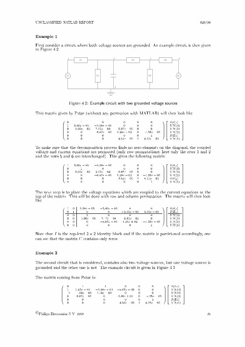
Example 1
First consider a circuit where both voltage sources are grounded. An example circuit is then givenin Figure 4.2.
1 2 3
0
E1
R1 R3
R2 R4
4R5
E2
Figure 4.2: Example circuit with two grounded voltage sources
This matrix given by Pstar (without any permution with MATLAB) will then look like
0BBBBB@
0 1 0 0 0 01 5:00e � 05 �5:00e� 05 0 0 00 �5:00e � 05 2:17e � 04 �6:67e� 05 0 00 0 �6:67e� 05 1:28e + 02 0 �4:55e� 050 0 0 0 0 10 0 0 �4:55e� 05 1 4:55e � 05
1CCCCCA
2666664
I(E2)V N(4)V N(3)V N(2)I(E1)V N(1)
3777775
To make sure that the decomposition process �nds no zero elements on the diagonal, the coupledvoltage and current equations are permuted (only row permutations; here only the rows 1 and 2and the rows 5 and 6 are interchanged). This gives the following matrix
0BBBBB@
1 5:00e � 05 �5:00e� 05 0 0 00 1 0 0 0 00 �5:00e � 05 2:17e � 04 �6:67e� 05 0 00 0 �6:67e� 05 1:28e + 02 0 �4:55e� 050 0 0 �4:55e� 05 1 4:55e � 050 0 0 0 0 1
1CCCCCA
2666664
I(E2)V N(4)V N(3)V N(2)I(E1)V N(1)
3777775
The next step is to place the voltage equations which are coupled to the current equations at thetop of the matrix. This will be done with row and column permutation. The matrix will then looklike
0BBBBB@
1 0 5:00e � 05 �5:00e � 05 0 00 1 0 0 �4:55e� 05 4:55e � 050 0 1 0 0 00 0 �5:00e � 05 2:17e � 04 �6:67e� 05 00 0 0 �6:67e � 05 1:28e + 02 �4:55e� 050 0 0 0 0 1
1CCCCCA
2666664
I(E2)I(E1)V N(4)V N(3)V N(2)V N(1)
3777775
Note that I is the top-level 2 � 2 identity block and if the matrix is partitioned accordingly, onecan see that the matrix C contains only zeros.
Example 2
The second circuit that is considered, contains also two voltage sources, but one voltage source isgrounded and the other one is not. The example circuit is given in Figure 4.3.
The matrix coming from Pstar is:
0BBBBB@
0 1 �1 0 0 01 1:67e � 04 �1:00e� 04 �6:67e� 05 0 0�1 �1:00e � 04 1:50e� 04 0 0 00 �6:67e � 05 0 5:00e + 01 0 �4:55e � 050 0 0 0 0 10 0 0 �4:55e� 05 1 4:55e � 05
1CCCCCA
2666664
I(E2)V N(3)V N(4)V N(2)I(E1)V N(1)
3777775
c Philips Electronics N.V. 1999 31

828/98 UNCLASSIFIED NATLAB REPORT
1 2 3
4
0
E1 E2
R1 R3
R2 R4
R5
Figure 4.3: Example circuit with one grounded voltage source
Row permutation, applied to the rows 1 and 2 and to the rows 5 and 6, to remove the zeros on thediagonal leads to:
0BBBBB@
1 1:67e � 04 �1:00e� 04 �6:67e� 05 0 00 1 �1 0 0 0�1 �1:00e � 04 1:50e� 04 0 0 00 �6:67e � 05 0 5:00e + 01 0 �4:55e � 050 0 0 �4:55e� 05 1 4:55e � 050 0 0 0 0 1
1CCCCCA
2666664
I(E2)V N(3)V N(4)V N(2)I(E1)V N(1)
3777775
Again placing the equations for V N(3) and V N(1) at the top of the matrix will lead to:
0BBBBB@
1 0 1:67e � 04 �1:00e � 04 �6:67e� 05 00 1 0 0 �4:55e� 05 4:55e � 050 0 1 �1 0 0�1 0 �1:00e � 04 1:50e � 04 0 00 0 �6:67e � 05 0 5:00e + 01 �4:55e � 050 0 0 0 0 1
1CCCCCA
2666664
I(E2)I(E1)V N(3)V N(4)V N(2)V N(1)
3777775
As can be seen, the voltage source E2, which is not grounded, gives a non-zero value within thematrix C. (Changing V N(3) with the other obvious choice, V N(4), gives a similar result.) Theother voltage source (grounded) only adds a empty column to matrix C.
The test circuits
Now consider the test circuits. The number of current equations is equal to the number of voltagesources. These values are presented in section 4.1. All voltage sources of all test circuits, exceptfor the circuit onebitadc, are grounded. It turns out that for all these circuits, matrix C is empty.For the circuit onebitadc, matrix C contains only one non-zero element, in the column belongingto the ungrounded voltage source.
The matrices created by Pstar, renumbered up-side-down and after the �rst row permutations,are called A. The matrix with the voltage equations of the voltage sources at the top of the ma-trix, is called matrix A1, thus A1 = PA1P
�1. Table 4.4 now shows the e�ects of these orderingsto the number of ops for the ILUT decomposition and the CGS algorithm. Note that the numberof ops needed if matrix A is used, is set on 100%. The �ll-in gives the percentage of non-zerosin the decomposed matrix. It contains the number of non-zeros of matrix U and matrix L. Thenumber of non-zeros of the decomposition of matrix A is set on 100%.
One can see that the number of ops decreases if matrix A is reordered according to matrix A1.Note that, as can be seen in Table 4.5, the number of CGS-iterations needed for a residual< 10�5
is only 1. The maximum of iterands needed for convergence (residual < 10�15) is 3, but within theNewton-Raphson process it is not needed that CGS gives a solution with a residual that is thatsmall. A residual of < 10�5 is accurately enough. (Note that in general the criteria for the linearsolver will depend on the Newton process.)Consider the di�erence in ops for the CGS method. As given in Chapter 3, the costs of the
32c Philips Electronics N.V. 1999

UNCLASSIFIED NATLAB REPORT 828/98
Matrix A Matrix A1
Name ILUT CGS �ll-in ILUT CGS �ll-in
onebitadc 100% 100% 100% 93% 98% 97%counter 100% 100% 100% 93% 99% 98%sram128 100% 100% 100% 67% 91% 77%dac5b 100% 100% 100% 80% 98% 98%er7899 100% 100% 100% 71% 97% 97%
Table 4.4: Comparison of the ops for two di�erent orders of variables
CGS method depends on the number of elements in the matrix. If the preconditioning matrices Land U contain more elements, then the preconditioning is more expensive. This will lead to morecomputations per iteration-step in the CGS method. However, in most cases, this is not the mainreason for the advantage caused by replacing some variables. As can be seen from table 4.4, thelargest part of the overall advantage comes from making the decomposition.
Depending on the coupling pattern of the circuit, some of the voltages equations have a signi�canthigher �ll-pattern in their rows than is the case for all the other variables. This can be explained bythe fact that some voltage sources in uence a large part of the circuit. The corresponding variablewill have a lot of connections with other variables. All the other variables are not connected thatmuch, thus their �ll-in of the row is much less. The di�erence between the �ll-in is very large(74% �ll-in towards 0:48% in case of the large circuits). This voltage source (in hierarchical largecircuits there are usually several of them) is always connected to the ground and therefore alwayshas a empty column in submatrix C of (4.4). By placing these equations at the top of the matrix,it will not be used for emptying the lower triangular matrix.This means that about 17% (the average of the percentage of the non-zero elements in these voltageequation toward the total number of non-zeros elements in the circuit matrices) of the non-zeroelements is not used in the decomposition process.
Before decomposition, Pstar makes sure that the order is set in such a way that the �ll-in of thematrices L and U is as low as possible. The only problem is that Pstar persists in treating thevoltage variables V N(i) and the belonging currents as a 2 � 2 block. Here improvement can beobtained to consider the row and column permutation as described above.
RemarkWhen dealing with hierarchical organised matrices (see Chapter 5), the above remarks apply tothe matrix of the circuit-level.
4.4.2 Eigenvalues
The CGS algorithm, without preconditioning, converges very badly in case of these circuit matrices.This can be explained by looking to the eigenvalues. As can be seen in Figure 4.4a, most of theeigenvalues are close to zero, which leads to a bad convergence, see Chapter 2. The picture that isshown represents the eigenvalues of the circuit onebitadc, but all the other circuits show a similarpattern. Note that some of the eigenvalues contain a small complex part. This is caused by theasymmetry of the system.If an ILUT-decomposition is used, matrix A will be split in two matrices: A = LU + R. If thedrop-tolerance � is equal to zero, the matrix R will be all zero and AU�1L�1 will be the identitymatrix. Now choose a value for � such that the �ll-in of the matrices U and L will decrease,but such that the matrix R will be as small as possible (then the preconditioned matrix is closeto the identity matrix and CGS will converge very fast). The eigenvalues of the preconditionedmatrix (using � = 10�4) are shown in Figure 4.4b. The di�erence in convergence speed betweena preconditioned matrix with eigenvalues close to 1 and an unpreconditioned matrix with theeigenvalues close to zero is shown in Figure 4.5.
c Philips Electronics N.V. 1999 33
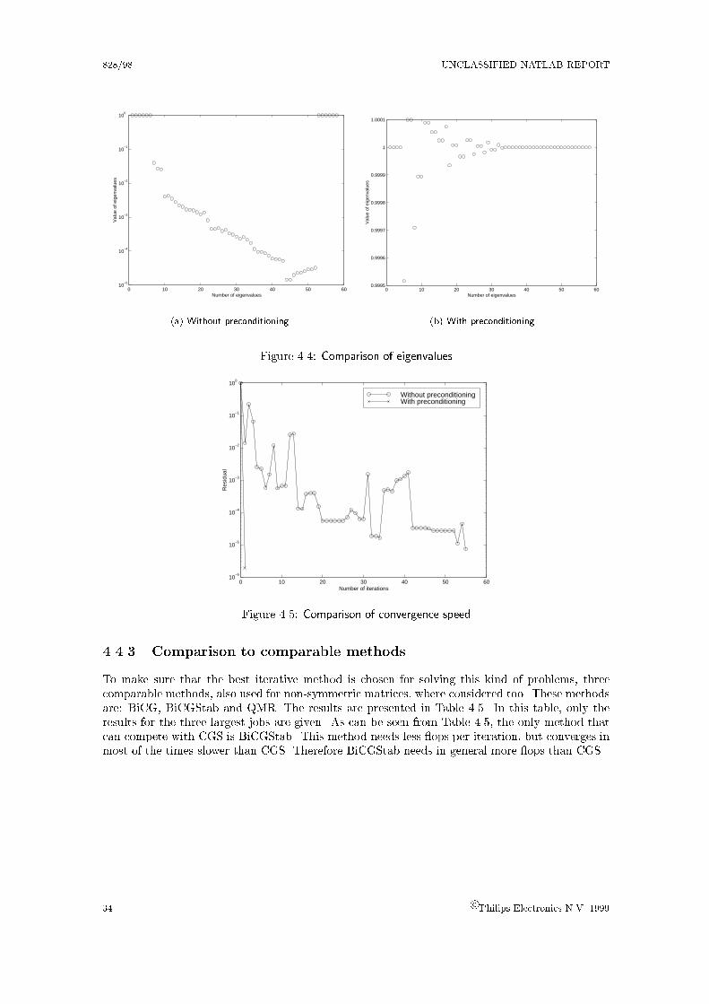
828/98 UNCLASSIFIED NATLAB REPORT
0 10 20 30 40 50 6010
−5
10−4
10−3
10−2
10−1
100
Number of eigenvalues
Val
ue o
f eig
enva
lues
(a) Without preconditioning
0 10 20 30 40 50 600.9995
0.9996
0.9997
0.9998
0.9999
1
1.0001
Number of eigenvalues
Val
ue o
f eig
enva
lues
(b) With preconditioning
Figure 4.4: Comparison of eigenvalues
0 10 20 30 40 50 6010
−6
10−5
10−4
10−3
10−2
10−1
100
Number of iterations
Res
idua
l
Without preconditioningWith preconditioning
Figure 4.5: Comparison of convergence speed
4.4.3 Comparison to comparable methods
To make sure that the best iterative method is chosen for solving this kind of problems, threecomparable methods, also used for non-symmetric matrices, where considered too. These methodsare: BiCG, BiCGStab and QMR. The results are presented in Table 4.5. In this table, only theresults for the three largest jobs are given. As can be seen from Table 4.5, the only method thatcan compete with CGS is BiCGStab. This method needs less ops per iteration, but converges inmost of the times slower than CGS. Therefore BiCGStab needs in general more ops than CGS.
34 c Philips Electronics N.V. 1999

UNCLASSIFIED NATLAB REPORT 828/98
Name Method # ops in % # iterations residual (b� Ax) error (x� A�1b)
sram128 CGS 100 1 1.46e-6 1.61e-3BiCGStab 80.3 1 1.10e-3 2.27e+0BiCG 213.2 2 1.90e-1 1.59e-3QMR 257.4 2 1.89e-1 1.59e-3GMRES 141.2 2 1.19e+1 1.60e-3
dac5b CGS 100 1 1.88e-6 7.35e-4BiCGStab 139.2 2 1.88e-6 7.06e-4BiCG 214.5 2 3.20e-6 1.31e-3QMR 259.5 2 3.20e-6 1.31e-3GMRES 137.6 2 3.58e-5 7.05e-4
er7899 CGS 100 1 4.92e-9 5.6e-7BiCGStab 139.7 2 2.69e-9 5.2e-7BiCG 212.9 2 8.52e-8 1.03e-6QMR 264.9 2 8.52e-8 1.03e-6GMRES 161.9 2 1.41e-7 5.20e-7
Table 4.5: Comparison iterative methods
c Philips Electronics N.V. 1999 35

Chapter 5
A hierarchical solver
The circuit simulation program Pstar, developed by Philips, transforms the electronic circuitsto equations as described in Chapter 2 and linearizes systems of non-linear equations by usingNewton-Raphson.In opposite to the systems considered in the previous chapters, Pstar uses a hierarchical construc-tion for the circuits. This hierarchy is described in section 5.1.To be able to use the iterative solver CGS, there needs to be a hierarchical version. In [14] alreadya hierarchical version of CGS with a preconditioner has been given. This is given in section 5.2and section 5.4. The preconditioner ILUT needs to be hierarchical as well. It is comparible to theUL-decomposition, which is already implemented in Pstar.
5.1 Hierarchical construction
Electronic circuits are often designed in a hierarchical way. This means that the circuit containsa couple of subcircuits, which is caused by the fact that designers link several circuits with knowncharacteristics. The top-level, most of the times called circuit level, consist of the elements that donot belong to one of the subcircuits. Note that these subcircuits can contain subcircuits themselves.The subcircuits are linked in the hierarchy by the boundary unknowns to the model at a higherlevel. At the circuit level, the �xed voltage at the ground node is the only boundary variable.Suppose now that a circuit contains one subcircuit. De�ne A1 as the matrix for the top level andA2 as the matrix for the subcircuit. The matrix A for the whole circuit is given in Figure 5.1.
A1
A2
A1+A2
A=
Figure 5.1: Structure of the complete circuit matrix
5.1.1 Example circuit
To illustrate the hierarchical construction, a simple example is shown.
Figure 5.2 shows the whole circuit without a hierarchical structure. In �gure 5.3 the hierarchicalstructure is shown. It is easy to see now that the unknowns 2 and 3 are interface unknowns andthe unknown 4 is the internal unknown of the subcircuit. The matrix formed by Pstar for the at
36
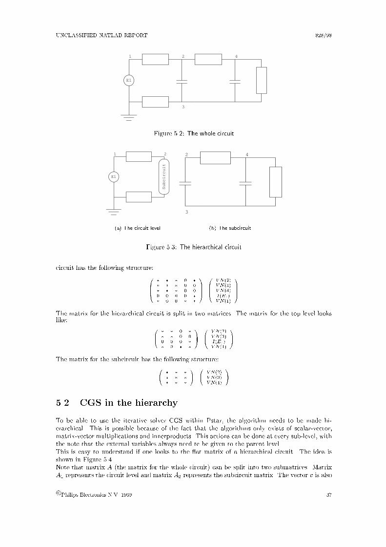
UNCLASSIFIED NATLAB REPORT 828/98
1 2
3
4
E1
Figure 5.2: The whole circuit
1 2
E1
Subcircuit
(a) The circuit level
2
3
4
(b) The subcircuit
Figure 5.3: The hierarchical circuit
circuit has the following structure:
0BBB@
� � � 0 �
� � � 0 0� � � 0 00 0 0 0 �
� 0 0 � �
1CCCA
0BBB@
V N(2)V N(3)V N(4)I(E1)V N(1)
1CCCA
The matrix for the hierarchical circuit is split in two matrices. The matrix for the top level lookslike:
0B@
� � 0 �
� � 0 00 0 0 �
� 0 � �
1CA
0B@
V N(2)V N(3)I(E1)V N(1)
1CA
The matrix for the subcircuit has the following structure:
0@
� � �
� � �
� � �
1A
0@
V N(2)V N(3)V N(4)
1A
5.2 CGS in the hierarchy
To be able to use the iterative solver CGS within Pstar, the algorithm needs to be made hi-erarchical. This is possible because of the fact that the algorithms only exists of scalar-vector,matrix-vector multiplications and innerproducts. This actions can be done at every sub-level, withthe note that the external variables always need te be given to the parent level.This is easy to understand if one looks to the at matrix of a hierarchical circuit. The idea isshown in Figure 5.4.Note that matrix A (the matrix for the whole circuit) can be split into two submatrices. MatrixA1 represents the circuit level and matrix A2 represents the subcircuit matrix. The vector v is also
c Philips Electronics N.V. 1999 37

828/98 UNCLASSIFIED NATLAB REPORT
A1
A2
v1
v2
A1+A2
Figure 5.4: The whole circuit
split into two parts, vector v1 and vector v2. The result of the computation Av for the common(boundary) values exists of A1v1 +A2v2.There are two hierarchical recursions possible: bottom-up or top-down. Because of the bottum-upprocedure of Pstar, the values of the boundary variables can only be counted if the values of A2v2are given to the parent level. The same procedure is (and needs to be) used for the matrix-vectorcomputations and the scalar-vector computations.Now it follows that it is quite important that after every computational step of the algorithmwithin a subcircuit, results are given to the parent circuit.For the hierarchical CGS, the method given in Table 3.3 will be split in several parts, where everypart is computed for all levels. The hierarchical algorithm for CGS is given in Table 5.1. Theorder of the algorithm di�ers a bit from the algorithm given in a previous chapter, but it is easierto implement it this way. This algorithm is also given in [14], section 4:2.As presented in the previous chapter, the method converges better when the matrix A is precon-ditioned with ILUT.
5.3 The hierarchical version of LU and ILUT decomposition
To be able to use the hierarchical construction, a suitable solver needs to be used. The standarddirect Gaussian method is one of the methods that can be used in a hierarchical environment.Starting with the submodels, one can combine the formation of the matrix and the (partial)decomposition by using a recursive bottom-up procedure. Finally, the blocks that correspond withthe boundary unknowns will be used for the matrix belonging to the model at a higher level.The solution process within a hierarchical structure will be considered more closely. Consider asystem of linear equations
Ax = b: (5.1)
Within Pstar, a UL-decomposition of the matrix A will be made, where U is an upper triangularmatrix and L is a lower triangular matrix. Assume that a matrix A belongs to a certain subcircuitwhich has n unknowns. The unknowns are numbered in such a way that the �rst k unknownvariables are the variables that couple this subcircuit to the model at a higher level. This means thatthere are n� k internal unknowns. These variables have, in contrast to the boundary unknowns,no connection with unknowns at a higher level and thus stay hidden for the higher levels.After computation of the local matrix in a hierarchical level, it is already possible to generate partsof the lower-triangular matrix L. The decomposition is started on the last row of the matrix. The
38c Philips Electronics N.V. 1999

UNCLASSIFIED NATLAB REPORT 828/98
x0 is the solution from the previous Newton iteration;r0 = b�Ax0, r�0 is taken arbitrary, such that (r0; r
�0) 6= 0
�0 = 1; p0 = q0 = 0for i = 1; 2; 3; : : :
� = �i�i�1
;
for each subcircuit:u = ri�1 + �qi�1;pi = u+ �(qi�1 + �pi�1);
end;� = 0;for each subcircuit:
v = Api;� = sigma+ (r�0 ; v);
end;� = �i
�;
for each subcircuit:qi = u� �v;u = u+ qi;xi = xi�1 + �u;
end;�i+1 = 0;for each subcircuit:
ri = ri�1 � �Au;�i+1 = �i+1 + (r�0 ; ri);
end;if xi is accurate enough, then quit;
end;
Table 5.1: The hierarchical CGS algortihm
last unknown is eliminated �rst from rows n� 1; : : : ; 1 of the linear set of equations on this level.This is done for all n� k internal unknowns. The blocks Ak , Lk and Ln�k are now known. Notethat the matrix Ln�k is lower triangular, where matrix Lk is normaly �lled.It is then not di�cult to show that the upper triangular matrix U can be found and is in facta by-product of the previous procedure. This will form a partial UL-decomposition of the formA = UL, with L given as
L =
�Ak 0Lk Ln�k
�:
On the higher level, only the resulting block Ak will be added to the local matrix on that higherlevel. After treating the top-level, a full UL-decomposition is formed (and the right-hand side ismultiplied by U�1). In practice one saves all elimination factors used to construct Ln�k in theupper triangle of L. Note that the matrix Ln�k is lower triangular, where matrix Lk is normaly�lled.Hence the decomposition is done by a bottom-up recursion. At the circuit level, the ground node isset to 0. The internal unknowns at that level follow from the lower triangular system. The valuesof the boundary variables will be past to each subcircuit at the next level. Thus the solution ofthe lower triangular systems is done by a top-down recursion.
Now consider the ILUT-decomposition. Because of the structure of Pstar, this decompositionwill also be replaced by IULT-decomposition. This decomposition is made the same way as theUL-decomposition extended with the dropping rules (for more information about this, see Chapter
c Philips Electronics N.V. 1999 39

828/98 UNCLASSIFIED NATLAB REPORT
2).
Within the hierarchy, it is quite di�cult to use the norm of the row, as needed for both droppingrules. In practice it turned out that using the diagonal element instead of the row-norm in thedropping rule, the result is at least as good as the result by using the row-norm. (These tests areconsidered for a at matrix after the I,V-row permutation.) This holds that the dropping ruleschange into:
A(i; j) = 0 if jA(i; j)j � � � jA(i; i)j; where � is given drop� tolerance: (5.2)
If all subcircuits and the top-level are decomposed, then the iterative method CGS can be usedand the matrix A will be preconditioned with U and L.
5.4 The preconditioned CGS in the hierarchy
In this section the results of preconditioning on the implementation will be given. The matrix Awill be copied into matrix K. This matrix K will be decomposed as described in the previoussection. The result is an upper triangular matrix U�1 and a lower trangular matrix L. Then thepreconditioning step U�1 � vector, where vector can be pi and ui, can be counted directly. On theother hand, L�1 is not directly availible. Therefore forward substitution needs to be done, whereLy = z needs to be counted, with y an auxilary vector and z = U�1 � vector. The hierarchicalalgorithm for the preconditioned CGS is based on the algorithm for preconditioned CGS for atmatrices, given in Table 3.4. This hierarchical algorithm is given in Table 5.2 (see also [14], section4:6).
40c Philips Electronics N.V. 1999
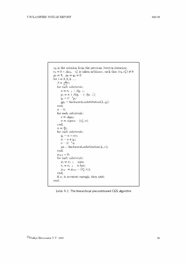
UNCLASSIFIED NATLAB REPORT 828/98
x0 is the solution from the previous Newton iteration;r0 = b�Ax0, r�0 is taken arbitrary, such that (r0; r
�0) 6= 0
�0 = 1; p0 = q0 = 0for i = 1; 2; 3; : : :
� = �i�i�1
;
for each subcircuit:u = ri�1 + �qi�1;pi = u+ �(qi�1 + �pi�1);qi = U�1pi;gpi = backward substitution(L; qi);
end;� = 0;for each subcircuit:
v = Agpi;� = sigma+ (r�0 ; v);
end;� = �i
�;
for each subcircuit:qi = u� �v;u = u+ qi;v = U�1u;gu = backward substitution(L; v);
end;�i+1 = 0;for each subcircuit:
xi = xi�1 + �gu;ri = ri�1 � �Agu;�i+1 = �i+1 + (r�0 ; ri);
end;if xi is accurate enough, then quit;
end;
Table 5.2: The hierarchical preconditioned CGS algorithm
c Philips Electronics N.V. 1999 41

Chapter 6
Conclusions
The performance of iterative solvers is studied when applied to systems arising in circuit simulation.In the �rst place, one can conclude that the iterative solver BGS is not a good solver for the circuitsimulation. In most of the cases that have been considered, the method converges very slowlyor is expensive in CPU-time. Several improvements are considered. However, even if vectorextrapolation is used to speed-up this convergence, the speed-up may be disappointing. Also arobust default de�nition of the parameters for vector extrapolation could not be found.It turned out that matrices of the test circuits, used for the investigations, are ill-conditioned (thecondition numbers are relativly high). This means that it is useful to use a preconditioner. Becauseof the fact that the preconditioner ILUT makes use of the numerical values instead of the structureof matrix A, this preconditioner is used.Tests turned out that the iterative solver CGS preconditioned with ILUT was the best solver forthe circuit matrices. The only methods that were compatible are GMRES and BiCGStab, butboth method needed more iterations to reach the same residual and therefore also more ops.The in uence of the order of the variables was also considered. It turned out that placing thevoltage variables belonging to the voltage sources at the top of the matrix increases the number of ops per iteration. In some cases the advantage was almost 25%.Unfortunately, it was not possible in the period of this study to implement this method, withchanging of the order of variables, into Pstar and thus to compare the hierarchical version withPstar's direct solver. For at, large circuit one would expect from the results in this reportthat this preconditioned CGS sould be able to give better results than the direct method (Thetestjobs considered here consisted of a large circuit with only transistor models in parallel thathad no internal unknowns). For the hierarchical circuits, a subcircuit must be quite large beforepreconditioned CGS is comparible to the direct solver. In practice, some mixture of methods mightbe necessary.Note that in the future, the option of Picard iteration instead of CGS within Transient-analysiscan be examined.
42

Appendix A
Branch equations
The branch constitutive equations for a number of basic elements:
Element Mode Branch Relation
Resistor DC, TR, AC V = R � II = V=R = G � V
Capacitor DC I = 0TR I = dQ(V )=dt
I = C(V )dV=dtAC I = jwCV
Inductor DC V = 0TR V = d�(I)=dt
V = L(I)dI=dtAC V = jwLI
43

Appendix B
Test circuits
Note that all structures that are shown correspond to matrices generated by Pstar, where a UL-decomposition is made. For the investigation described before, all matrices are reversed.
B.1 Onebitadc
It is a 1 bit analog to digital converter. The circuit is small and hierarchical. The circuit consistsof 6 voltage sources, where one is not grounded and the rest is grounded, NMOS- and PMOStransistors and a number of juncaps (spread diodes).There are 7 submodels which create a total hierarchical depth of 6. The at, linear system has adimension of 58. The total number of non-zeros is 435. The maximum of non-zeros in a row is 44and the minimum is 1. The structure of the coe�cient matrix A is shown in Figure B.1.
0 10 20 30 40 50
0
10
20
30
40
50
Figure B.1: Stucture of matrix A
44

UNCLASSIFIED NATLAB REPORT 828/98
B.2 Counter
The circuit is a 10 bit binair counter with backward coupling. It is a small, at circuit withoutprocess bloc. The circuit consists of 3 voltage sources (all grounded) and NMOS- and PMOStransistors. It does not hold parasites (diodes or capacitors).The circuits has no submodels, which leads to a hierarchical depth of 2. The matries of thesubsystems for NMOS- and PMOS transistors do not require a partial Gaussian elimination in thelower hierarchical level. Hence, in this example, the matrix at the circuit level is identical to the at matrix.The linear system has a dimension of 96. The total number of non-zeros is 783. The maximum ofnon-zeros in a row is 74 and the minimum is 1. The structure of the coe�cient matrix A is shownin Figure B.2.
0 10 20 30 40 50 60 70 80 90
0
10
20
30
40
50
60
70
80
90
Figure B.2: Stucture of matrix A
c Philips Electronics N.V. 1999 45

828/98 UNCLASSIFIED NATLAB REPORT
B.3 Sram128
It is a RAM-memory en contains a few tables which can de�ne voltage sources. It consists of 29voltage sources (all grounded) and capacitors. Within the DC-analysis, the capacitors are bypassedwith resistors. This is done by using G+�C in stead of G, where � is small to avoid oating areas.The circuits has no submodels, which leads to a hierarchical depth of 2. The linear system has adimension of 2624. The total number of non-zeros is 35823. The maximum of non-zeros in a rowis 2571 and the minimum is 1. The structure of the coe�cient matrix A is shown in Figure B.3.
Figure B.3: Stucture of matrix A
46 c Philips Electronics N.V. 1999
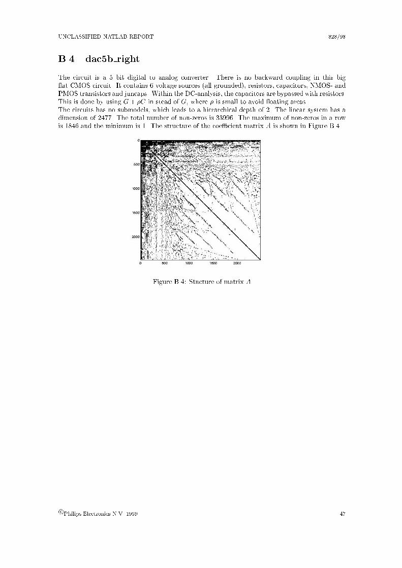
UNCLASSIFIED NATLAB REPORT 828/98
B.4 dac5b right
The circuit is a 5 bit digital to analog converter. There is no backward coupling in this big at CMOS circuit. It contains 6 voltage sources (all grounded), resistors, capacitors, NMOS- andPMOS transistors and juncaps. Within the DC-analysis, the capacitors are bypassed with resistors.This is done by using G+ �C in stead of G, where � is small to avoid oating areas.The circuits has no submodels, which leads to a hierarchical depth of 2. The linear system has adimension of 2477. The total number of non-zeros is 33996. The maximum of non-zeros in a rowis 1846 and the minimum is 1. The structure of the coe�cient matrix A is shown in Figure B.4.
Figure B.4: Stucture of matrix A
c Philips Electronics N.V. 1999 47

828/98 UNCLASSIFIED NATLAB REPORT
B.5 ER 7899
It is a 9 bit digital to analog converter. The 9 digital entries are quite stable. There is nobackward coupling in this at circuit. The circuit consists of 16 voltage sources (all grounded),resistors, capacitors, NMOS- and PMOS transistors and juncaps. Within the DC-analysis, thecapacitors are bypassed with resistors.The circuits has 10 submodels, which create a hierarchical depth of 3. The linear system has adimension of 2612. The total number of non-zeros is 26260. The maximum of non-zeros in a rowis 1846 and the minimum is 1. The structure of the coe�cient matrix A is shown in Figure B.5.
Figure B.5: Stucture of matrix A
48 c Philips Electronics N.V. 1999

Appendix C
Coupling factor and partitioning
The intention to look at another method than the methods that are already used in Pstar, is thepossibility to simulate large digital systems which contain many MOS-transistors in a much fasterway.Within Pstar, the main method to solve a system of equations is the LU-decomposition.Due to an earlier study (results can be found in [10, 11]), the block Gauss-Seidel (BGS) is a methodthat can work quite well as a linear solver within Transient-analysis.In Pstar, BGS has been implemented in the circuit level only. Within the test set of Pstar thereare only two jobs, that use this BGS-method. The �rst one exists of about 5000 transistors andthe second one exists of 1000 transistors. BGS is also used for the additional job ER 7899. Insteadof a much smaller CPU-time, the problem needed much more simulation time when compared toordinary Gaussian elimination within transient analysis. This job exists of about 4000 transistorsand therefore it would be useful to use BGS. For job ER 7899 the performance of BGS was improvedusing a lower value of coupling factor � and after a correction of the stopping criterion (see also [6]).
C.1 Dynamic partitioning
There are several techniques to partition a circuit. Two possible kinds of partitioning are
1. static partitioning and
2. dynamic partitioning.
In this section, the only partitioning that will be considered is the dynamic partitioning. The staticpartitioning is described in [10].
A dynamic partioning is a partitioning of the circuit made during the simulation. One of themethods that is used within several circuit simulators is the coupling based partitioning. The mainidea of this method is to �nd tightly couplings by using a certain formula. After that, all the tightlycoupled nodes (or variables) are placed in a tightly coupled variable list. This way of partitioningis based on diagonally dominance of the matrix. As been said in the training report [6], diagonaldominance is a condition to guarantee convergence of the usual GS. If a 2 � 2-submatrix causesnon-diagonally dominance, the associated variables will be called strongly coupled. (The ones thatsatisfy diagonally dominance can be solved by usual GS and will be placed in a weakly coupledpair list.)The negation of diagonally dominance is :(jaiij >
Pj 6=i jaij j) or better
9ijaiij �Xj 6=i
jaiij (C.1)
49
828/98 UNCLASSIFIED NATLAB REPORT
For a 2� 2-submatrix, the right-hand side of the inequality C.1 will be reduced to jaij j, which willsimply lead to jaiij � jaij j. If two nodes satisfy this condition, then they are said to have a strongcoupling from node i to node j.
Now there are two possible ways of de�ning strongly coupled pairs.
(i) In the �rst criterion there must be a strong coupling from node i to node j and from node jto node i. So, it holds that
jaij j � jaiij ^ jajij � jajj j (C.2)
or even better is:
jaij j > jaiij ^ jajij > jajj j: (C.3)
To be able to in uence the coupling a bit more, a certain bound � is introduced as followsjaij j > �jaiij. This will lead to :
jaij j > � jaiij ^ jajij > � jajj j: (C.4)
The value � must satisfy 0 < � < 1. Within Pstar, � is standard chosen as � = 0:5, but it isa so-called change parameter, which means that it can be changed by the user. Within theiteration process, it is not possible to change the value of �. If a lower value of � is taken, thenumber of iterations to reach convergence will decrease. A better default value for � wouldbe � = 0:1.
(ii) The second criterion is based on the idea that there only needs to be a strong coupling in onedirection. If that is true, then the two nodes are coupled strongly. Written in equation formit will give:
jaij j > �jaiij _ jajij > �jajj j: (C.5)
The two criterions are almost the same and will lead (if the coupling factor is smal enough) tothe same subcircuits. The second criterion will sometimes make larger subcircuits for the samecoupling factor. The value of � may vary, but is bounded by an upper and lower bound: 0 < � < 1.If � is near to zero or one all variables will be considered as respectively strongly or weakly coupled,and then the advantage of the block method will disppear.The blocks will be formed by clustering these pairs. A simple algorithm starts by checking whethertwo pairs have a variable in common. If so, place them in the same subcircuit, S1, otherwise maketwo subcircuits of it, S1 and S2. Apply this algorithm to all pairs of strongly coupled variablesand to all subcircuits constructed so far. In the end, there will be a partitioning of all variables ina number of disjoint subcircuits. The set of all subset will be given by
S(�) = fSj9N : S = fS1; :::; SNg;[Ni=1Si = All;8i;jSi \ Sj = ;g:Note that for each �0 it holds that there is an neighbourhood U�0
of �0 such that each � in thatneighbourhood forms the same subsets. There is a �nite number of U�0
that form a partition of[0; 1]. Because of the fact that there will exists �� < � < �+, that will give di�erent blocks thanS(�), it is possible to approximate �� and �+, with �� < � < �+, such that S(��) 6= S(�) 6=S(�+). While determing S(�), one can easily �nd approximations for �� and �+ at the sametime.
C.2 Adaptive coupling factor
An extra functionality which could be implemented easily in Pstar is an adaptively-determinedcoupling factor. It might be useful to be able to change the coupling factor during the iteration
50 c Philips Electronics N.V. 1999

UNCLASSIFIED NATLAB REPORT 828/98
proces. Start with a standard coupling factor, say � = 0:5. During the iteration proces there aretwo factors that can in uence the value of the coupling factor, the convergence speed and the blocksize. While considering the convergence speed, Pstar can check whether the convergence speed ishigh enough. (This can be done by approximation of the spectral radius cf below.) If not, a smallercoupling factor can be used to make new partitionings using larger blocks.If the block size is used, Pstar needs to check whether the bocks are not too large. If the blocksare too large, then a larger value of � needs to be chosen, because otherwise the advantage of theusage a block method will be lost.At a certain moment, the increase of the computations will be more than the decrease of the num-ber of iterations. Finally this will lead to a larger analysis time (or CPU time). If it is possible,there must be found an optimum between the spectral radius (which depends on the couplingfactor) and the CPU-time.
c Philips Electronics N.V. 1999 51

828/98 UNCLASSIFIED NATLAB REPORT
Given in quasi-implementation, this will look like:
Constants: �def , sizemax, sizemin, �def� = �def ;Determine S(�), �� and �+.Determine also the size of the individual blocks (size).if size < sizemax
fif size > sizeminf Determine �(�);if �(�) < �def fcontinue gelse f�+ := � ; � := ��;
determine S(�) and ��g
gelse f �+ := � ; � := ��;
determine S(�) and ��g
gelse f �� := � and � := �+;
determine S(�) and �+g
The spectral radius �(�) can be determined within the iteration process by using the followingapproxiation:
�(�) = (residuala
residualb)
1a�b ; (C.6)
where b < a and residuala represents the residual after a iterations.
52 c Philips Electronics N.V. 1999
Bibliography
[1] O. Axelsson and V.A. Barker,Finite element solution of boundary value problems
1984, Academic Press, Inc. Orlando.
[2] R. Barker, M. Berry, T. Chan, J, Demmel, J. Donato, J. Dongarra, V. Eijkhout, R. Pozo, C.Omine, H. van der Vorst,Templates, for the solution of linear systems: building blocks for iterative methods
1994, SIAM, Philadelphia.
[3] J.W. Francke,A block preconditioning method in circuit simulation
1994, Natlab Technical Note 195, Philips Electronics N.V. Eindhoven.
[4] W. Hackbusch,Iterative L�osung grosser schwachbesetzter Gleichungssysteme
1991, Teubner Studienb�ucher Mathematik, vol.69.
[5] A.J.M. Huijben and E.J.W. ter Maten,Vector extrapolation applied to a time-cyclic heat problem
1992, Natlab Technical Note 189, Philips Electronics N.V. Eindhoven.
[6] L.S. Lengowski,Block Gauss-Seidel prestudy project
1998, Eindhoven Technical University.
[7] MATLAB,High performance numeric computation and visualization software
1998, Version 5.2.0, The MathWorks, Inc.
[8] W.J. McCalla,Fundamentals of computer-aided circuit simulation
1988, Kluwer Academic Publischers, Boston.
[9] L.W. Nagel,SPICE2, A computer program to simulate semiconductor circuits
1975, Report No ERL-M520, College of Engeneering, University of California, Berkely.
[10] T.P. Nguyen,A hybrid method for solving systems of nonlinear circuit equations: combining relaxation
methods with direct methods
1993, Natlab Technical Note 204, Philips Electronics N.V. Eindhoven.
[11] T.P. Nguyen,A dynamic circuit partitioning and iterative method for circuit simulation
1994, Natlab Report 6823, Philips Electronics N.V. Eindhoven.
53

828/98 UNCLASSIFIED NATLAB REPORT
[12] Pstar User Guide (available from ED&T),Philips Electronics N.V. Eindhoven.
[13] Y. Saad,Iterative methods for sparse linear systems
1996, PWS Publishing comp., Boston.
[14] W.H.A. Schilders and M.M.A. Driessen,Iterative linear solvers for circuit simulation
1995, Natlab Report 6854, Philips Electronics N.V. Eindhoven.
[15] W.H.A. Schilders,Numerical methods for semiconductor device simulation, Volume 1
1998, Philips Electronics N.V. Eindhoven.
[16] M.F. Sevat, T.J. Engelen, J.C.H van Gerwen and E.J.W. ter Maten,Harmonic balance algorithm in Pstar
1998, Version 2.0, Internal Doc. Philips ED&T/AS, Philips Electronics N.V. Eindhoven.
[17] A. Sidi,Extrapolation vs. projection methods for linear systems of equations
1987, Israel Institute of Technology.
[18] A. van der Sluis,Memo on vector extrapolation
1992.
[19] P. Sonneveld,CGS, a fast Lanczos-type solver for non-symmetric linear systems
1989, SIAM J. SCI. STAT. COMPUT., Vol. 10.
[20] J. Stoer and R. Bulirsch,Introduction to numerical analysis
1993, Springer-Verlag New York, Inc.
[21] R.S. Varga,Matrix iterative analysis
1962, Prentice-Hall International, London.
[22] H.A. van der Vorst,Lecture notes on iterative methods
1992, Report TR/PA/G2/75, CERFACS, Toulouse.
[23] D.M. Young,Iterative solution of large linear systems
1971, Academic Press, New York and London.
54 c Philips Electronics N.V. 1999

UNCLASSIFIED NATLAB REPORT 828/98
Author(s) Linda Lengowski
Title CGS preconditioned with ILUT as a solver for circuit simulationMaster Thesis
Distribution
Nat.Lab./PI WB-5PRL Redhill, UKPRB Briarcli� Manor, USALEP Limeil{Br�evannes, FrancePFL Aachen, BRDCP&T WAH
Director: Dr. Ir. M.F.H. Schuurmans WB-56Deputy Director a.i.: Ir. E. Roza WAY-52Department Head: Ir. G.F.M. Beenker WAY-32
Abstract
Ir. H.A.J. van de Donk PRLE, ED&T WAY-31Dr. H.H.J. Janssen PRLE, ED&T WAY-31Dr. Ir. T.A.M. Kevenaar PRLE, ED&T WAY-31Ir. M.F. Sevat PRLE, ED&T WAY-31Dr. T.G.A. Heijmen PRLE WAY-41Ir. M. Stoutjesdijk PS-CIC Nijmegen
Full report
Ir. J.G. Fijnvandraat PRLE, ED&T WAY-31Ir. J.C.H. van Gerwen PRLE, ED&T WAY-31Dr. E.J.W. ter Maten PRLE, ED&T WAY-31Dr. Ir. S.P. Onneweer PRLE, ED&T WAY-31Ir. J.M.F. Peters PRLE, ED&T WAY-31Mw. Drs. E.J.M. Duren-van der AA PRLE, ED&T WAY-31Mw. Drs. M.M.A. Driessen PRLE, ED&T WAY-31Ing. T.P. Nguyen PS-Microtel WAY-31Mw. L.S. Lengowski PRLE, ED&T WAY-31S.H.M.J. Houben PRLE, ED&T WAY-41Dr. Ir. P.B.L. Meijer PRLE WAY-41Ir. C. Niessen PRLE WAY-41Dr. W.H.A. Schilders PRLE WAY-41Drs. M.C.J. van de Wiel PS-ASG-LTC BQ1, NijmegenProf. Dr. H.A. van der Vorst PRLE (advisor) Utrecht University
Mathematical InstituteP.O.Box 800103508 TA Utrecht
Prof. dr. R.M.M. MattheijDr. E.F. KaasschieterDr. J.M.L. Maubach Eindhoven Technical University
Dept. of Mathematics and Computing Science, HG8P.O. Box 5135600 MB Eindhoven
c Philips Electronics N.V. 1999 55

828/98 UNCLASSIFIED NATLAB REPORT
56 c Philips Electronics N.V. 1999