An efficient, preconditioned, high-order solver for scattering by two-dimensional inhomogeneous...
25
An efficient, preconditioned, high-order solver for scattering by two-dimensional inhomogeneous media Oscar P. Bruno a,1 , E. McKay Hyde b, * ,2 a Applied and Computational Mathematics, Caltech, Pasadena, CA 91125, USA b School of Mathematics, University of Minnesota, 127 Vincent Hall, 206 Church Street SE, Minneapolis, MN 55455, USA Received 31 October 2003; received in revised form 29 April 2004; accepted 29 April 2004 Available online 8 June 2004 Abstract We consider the problem of evaluating the scattering of TE polarized electromagnetic waves by two-dimensional penetrable inhomogeneities: building upon previous work [IEEE Trans. Antennas Propag. 48 (2000) 1862] we present a practical and general fast integral equation algorithm for this problem. The contributions introduced in this text in- clude: (1) a preconditioner that significantly reduces the number of iterations required by the algorithm in the treatment of electrically large scatterers, (2) a new radial integration scheme based on Chebyshev polynomial approximation, which gives rise to increased accuracy, efficiency and stability, and (3) an efficient and stable method for the evaluation of scaled high-order Bessel functions, which extends the capabilities of the method to arbitrarily high frequencies. These enhancements give rise to an algorithm that is much more accurate and efficient than its previous counterpart, and that allows for treatment of much larger problems than permitted by the previous approach. In one test case, for example, the present algorithm results in far-field errors of 8:9 10 13 in a 2.12s calculation (on a 1.7 GHz PC) whereas the original algorithm gave rise to far-field errors of 1:1 10 8 in 88.91s on a 400 MHz PC. In another example, the present algorithm evaluates accurately the scattering by a cylinder of acoustical size jR ¼ 256, which is of the order of 20 times larger (400 times larger in square wavelengths) than the largest scatterers that could be treated by the previous ap- proach. Yielding, at worst, third-order far field accuracy (or substantially better, for smooth scatterers) in fast com- puting times (OðN log N Þ operations for an N point mesh) even for discontinuous and complex refractive index distributions (possibly containing severe geometric singularities such as corners and cusps), the proposed approach is the highest-order OðN log N Þ solver in existence for the problem under consideration. Ó 2004 Elsevier Inc. All rights reserved. AMS: 35J05; 65D30; 65F10; 65N12; 65R20; 65T50; 78A45; 78M25 * Corresponding author. Tel.: +1-612-624-5895; fax: +1-612-626-2017. E-mail address: [email protected] (E.M. Hyde). 1 Supported by the AFOSR under Grant Nos. F49620-96-1-0008, F49629-99-1-0010 and F49620-02-10049, by the NSF through the NYI award DMS-9596152 and contract Nos. DMS-9523292, DMS-9816802 and DMS-0104531 and by the Powell Research Foundation. 2 Supported through a DOE Computational Science Graduate Fellowship, an Achievement Reward for College Scientists (ARCS) Fellowship and an NSF Mathematical Sciences Postdoctoral Research Fellowship. 0021-9991/$ - see front matter Ó 2004 Elsevier Inc. All rights reserved. doi:10.1016/j.jcp.2004.04.017 www.elsevier.com/locate/jcp Journal of Computational Physics 200 (2004) 670–694
-
Upload
independent -
Category
Documents
-
view
7 -
download
0
Transcript of An efficient, preconditioned, high-order solver for scattering by two-dimensional inhomogeneous...
www.elsevier.com/locate/jcp
Journal of Computational Physics 200 (2004) 670–694
An efficient, preconditioned, high-order solver for scatteringby two-dimensional inhomogeneous media
Oscar P. Bruno a,1, E. McKay Hyde b,*,2
a Applied and Computational Mathematics, Caltech, Pasadena, CA 91125, USAb School of Mathematics, University of Minnesota, 127 Vincent Hall, 206 Church Street SE, Minneapolis, MN 55455, USA
Received 31 October 2003; received in revised form 29 April 2004; accepted 29 April 2004
Available online 8 June 2004
Abstract
We consider the problem of evaluating the scattering of TE polarized electromagnetic waves by two-dimensional
penetrable inhomogeneities: building upon previous work [IEEE Trans. Antennas Propag. 48 (2000) 1862] we present a
practical and general fast integral equation algorithm for this problem. The contributions introduced in this text in-
clude: (1) a preconditioner that significantly reduces the number of iterations required by the algorithm in the treatment
of electrically large scatterers, (2) a new radial integration scheme based on Chebyshev polynomial approximation,
which gives rise to increased accuracy, efficiency and stability, and (3) an efficient and stable method for the evaluation
of scaled high-order Bessel functions, which extends the capabilities of the method to arbitrarily high frequencies. These
enhancements give rise to an algorithm that is much more accurate and efficient than its previous counterpart, and that
allows for treatment of much larger problems than permitted by the previous approach. In one test case, for example,
the present algorithm results in far-field errors of 8:9� 10�13 in a 2.12s calculation (on a 1.7 GHz PC) whereas the
original algorithm gave rise to far-field errors of 1:1� 10�8 in 88.91s on a 400 MHz PC. In another example, the present
algorithm evaluates accurately the scattering by a cylinder of acoustical size jR ¼ 256, which is of the order of 20 times
larger (400 times larger in square wavelengths) than the largest scatterers that could be treated by the previous ap-
proach. Yielding, at worst, third-order far field accuracy (or substantially better, for smooth scatterers) in fast com-
puting times (OðN logNÞ operations for an N point mesh) even for discontinuous and complex refractive index
distributions (possibly containing severe geometric singularities such as corners and cusps), the proposed approach is
the highest-order OðN logNÞ solver in existence for the problem under consideration.
� 2004 Elsevier Inc. All rights reserved.
AMS: 35J05; 65D30; 65F10; 65N12; 65R20; 65T50; 78A45; 78M25
*Corresponding author. Tel.: +1-612-624-5895; fax: +1-612-626-2017.
E-mail address: [email protected] (E.M. Hyde).1 Supported by the AFOSR under Grant Nos. F49620-96-1-0008, F49629-99-1-0010 and F49620-02-10049, by the NSF through the
NYI award DMS-9596152 and contract Nos. DMS-9523292, DMS-9816802 and DMS-0104531 and by the Powell Research
Foundation.2 Supported through a DOE Computational Science Graduate Fellowship, an Achievement Reward for College Scientists (ARCS)
Fellowship and an NSF Mathematical Sciences Postdoctoral Research Fellowship.
0021-9991/$ - see front matter � 2004 Elsevier Inc. All rights reserved.
doi:10.1016/j.jcp.2004.04.017
O.P. Bruno, E.M. Hyde / Journal of Computational Physics 200 (2004) 670–694 671
Keywords: Helmholtz equation; Lippmann–Schwinger equation; FFT; TE/TM scattering; Preconditioner; Chebyshev polynomials;
Bessel functions
1. Introduction
Scattering problems find application in a wide range of fields including communications, materials
science, plasma physics, biology and medicine, radar and remote sensing. The evaluation of useful nu-
merical solutions to such problems remains a challenge, requiring novel mathematical approaches andpowerful computational tools. In this paper, building on the contribution of [1,2], we present a practical
and general integral equation algorithm for the evaluation of time-harmonic, TE polarized electromagnetic
scattering by bounded inhomogeneities in two dimensions. (Note that there is some ambiguity in the
naming of the polarization with some authors referring to this setting as TM polarized scattering; see [3–6].
To be precise, we consider the case in which the electric field is parallel to the cylindrical axis of the
scatterer.)
Our problem can be stated as follows: given an incident field ui, satisfying Dui þ j2ui ¼ 0, we denote by uthe total electric field – which equals the sum of ui and the resulting scattered field us: u ¼ ui þ us. Therefractive index of the scattering obstacle is given by a bounded (possibly discontinuous) function nðxÞ,where nðxÞ ¼ 1 outside some compact set X. Calling k the wavelength of the incident field and j ¼ 2p=k the
wavenumber, the total field u satisfies [7, p. 2]
Duþ j2n2ðxÞu ¼ 0; x 2 R3: ð1Þ
Finally, the scattered field, us, is required to satisfy the Sommerfeld radiation condition [7, p. 67]
limr!1
ffiffir
p ous
or
�� ijus
�¼ 0: ð2Þ
An appropriate integral formulation for our two-dimensional TE problem is given by the Lippmann–
Schwinger equation [7, p. 214]
uðxÞ ¼ uiðxÞ � j2
ZXgðx� yÞmðyÞuðyÞ dy; ð3Þ
where gðxÞ ¼ ði=4ÞH 10 ðjjxjÞ is the fundamental solution for the Helmholtz equation in two dimensions and
m is the compactly supported function m ¼ 1� n2. For the present problem, integral equation methods have
a number of advantages over, say, finite element methods; in particular, the integral approaches only re-
quire discretization of the equation on the scatterer itself (the region surrounding the scatterer needs not be
discretized), and the solutions they produce satisfy the radiation condition at infinity automatically (no
absorbing boundary conditions are needed). Direct use of integral equation methods is costly, however,since they lead to dense linear systems of equations: a straightforward computation of the required con-
volution requires OðN 2Þ operations per iteration of an iterative linear solver – where N is the number of
mesh points in the discretization. As in other Fourier-based integral methods [8], however, in our integral
equation approach the complexity of the convolution evaluation is reduced to OðN logNÞ operations periteration. In addition, our method achieves higher-order accuracy, yielding, at worst, far-field errors of
order Oðh3Þ, even for discontinuous and rather complex refractive index distributions – possibly containing
geometric singularities such as corners and cusps, which present severe difficulties for other methods. This
compares favorably with previous approaches, which either require OðN 2Þ operations per iteration or, if

672 O.P. Bruno, E.M. Hyde / Journal of Computational Physics 200 (2004) 670–694
applicable in OðN logNÞ operations per iteration, yield lower orders of accuracy than our approach – no
better than Oðh2ð1þ logðhÞÞÞ accuracy for discontinuous refractive indexes [8–12] (see [13] for a more
detailed comparison of various algorithms for the problem under consideration).Following [1,2], our method is based on recasting the integral term of (3) in the polar coordinate form
ðKuÞða;/Þ ¼ �j2
Zgða;/; r; hÞmðr; hÞuðr; hÞr dr dh: ð4Þ
An approximate integral equation is obtained from (4) by replacing the fundamental solution g by a
truncation of its Fourier representation with respect to the angular variables (given by the addition theorem
for the Hankel function [7, p. 67]). Denoting the solution of the approximate integral equation by v, wehave
vða;/Þ ¼ ui;Mða;/Þ þ ðKMvÞða;/Þ; ð5Þ
where
ui;Mða;/Þ ¼XM‘¼�M
ui‘ðaÞei‘/; ð6Þ
ðKMvÞða;/Þ ¼XM‘¼�M
ðK‘vÞðaÞei‘/: ð7Þ
Here, using an annular region R0 6 a6R1 containing the support of m, the operator K‘ is defined by
ðK‘vÞðaÞ ¼ � ij2
4
Z R1
R0
J‘ða; rÞI‘ðrÞr dr; ð8Þ
where calling J‘ and H 1‘ the Bessel and Hankel functions of order ‘,
J‘ða; rÞ ¼ H 1‘ ðjmaxða; rÞÞ J‘ðjminða; rÞÞ ð9Þ
and
I‘ðrÞ ¼Z 2p
0
mðr; hÞvMðr; hÞe�i‘h dh: ð10Þ
From (5) it is clear that v ¼ vM , i.e., the approximate solution v is itself a truncated Fourier series.
(Throughout this paper we use a superscript M to denote the truncated Fourier series of order M of a given
function.)
Remark 1. Note that the polar coordinate formulation in no way restricts our algorithm to cylindrically
symmetric scatterers; indeed, the algorithm can treat a completely general collection of bounded penetrable
inhomogeneities. Further, the polar coordinate formulation is particularly well adapted for use in a number
of important applications. In particular, fiber optics problems often require the solution of the Helmholtz
equation (1) within a disc [14].
In [15,13] we proved that Eq. (5) admits a unique solution vM for piecewise-smooth inhomogeneities m,and that vM provides a high-order approximation to the solution u of (3) (see [13] for a more precisedefinition of the appropriate spaces and a more precise statement of the results). In particular, for a dis-
continuous and piecewise-smooth inhomogeneity m, the L1 error decays as OðM�3Þ in the far field and as
O.P. Bruno, E.M. Hyde / Journal of Computational Physics 200 (2004) 670–694 673
OðM�2Þ in the near field; furthermore, the order of convergence increases rapidly with the degree of reg-
ularity of m.Like the algorithm of [1,2], the method presented in this paper is based on consideration of the polar
coordinate formulation (5). The contributions introduced in this text include: (1) a new radial integration
scheme based on Chebyshev polynomial approximations, which gives rise to increased accuracy, efficiency
and stability (Section 3), (2) an efficient and stable method for the evaluation of scaled high-order Bessel
functions, which extends the capabilities of the method to arbitrarily high frequencies (Section 4), and (3) a
preconditioner that significantly reduces the number of iterations required by the algorithm in the treatment
of electrically large scatterers (Section 5). These enhancements give rise to an algorithm that is much more
accurate and efficient than its previous counterpart, and that allows for treatment of much larger problems
than permitted by the previous approach. In one test case, for example, the present algorithm results in far-field errors of 8:9� 10�13 in a 2:12s calculation (on a 1.7 GHz PC) whereas the original algorithm gave rise
to far-field errors of 1:1� 10�8 in 88:91s on a 400 MHz PC. In another example we evaluate scattering by a
cylinder of acoustical size jR ¼ 256, which of the order of 20 times larger (400 times larger in square
wavelengths) than the largest scatterers that could be treated by the previous approach. A variety of nu-
merical examples illustrating the efficiency and accuracy of the method, including applications to refractive
index distributions containing complex geometric singularities, are presented in Section 6.
2. High-order angular integration
For high-order, OðN logNÞ evaluation of the quantities I‘ðrÞ in Eq. (10) we proceed as in [2]: in terms of
the Fourier coefficients of the inhomogeneity m and the approximate solution vM we have
I‘ðrÞ ¼Z 2p
0
X1j¼�1
mjðrÞeijh ! XM
k¼�M
vkðrÞeikh !
e�i‘h ¼ 2pXMk¼�M
m‘�kðrÞvkðrÞ; ð11Þ
where ‘ ¼ �M ; . . . ;M . Hence, at each radius r, I‘ðrÞ is given by a finite convolution of the Fourier coef-
ficients m‘ðrÞ and v‘ðrÞ involving Fourier modes of m of orders j‘j6 2M . In our method these convolution
are evaluated by a well-known FFT algorithm [16, pp. 531–537] at a computational cost of OðM logMÞ foreach radius. Therefore, given the finitely many Fourier coefficients m‘ðrÞ and v‘ðrÞ in (11), we can compute
the angular integrals I‘ðrÞ exactly (except for roundoff errors) in a total of OðNrM logMÞ ¼ OðN logNÞoperations, where Nr denotes the number of radial discretization points and N ¼ Nrð2M þ 1Þ denotes thetotal number of unknowns.
Note the following interesting implication of (11): the high-order modes of m (m‘ for j‘j > 2M) do not
enter the calculation of I‘. It follows that the function m can be replaced by the smooth function m2M with no
effect on the accuracy of I‘. Similarly, it is not difficult to see that, after first replacing m by m2M , evaluation
of the convolutions (11) is exactly equivalent to trapezoidal rule integration of (10) with Nh > 4M inte-
gration points. More precisely,
I‘ðrÞ ¼ INh‘ ðrÞ �
XNh�1
j¼0
m2Mðr; hjÞvMðr; hjÞe�2pij‘=Nh ; ð12Þ
where hj ¼ 2pj=Nh for j ¼ 0; 1; . . . ;Nh � 1. We thus compute INh‘ ðrÞ using FFTs in a total of OðN logNÞ
operations.
Although I‘ðrÞ may always be computed exactly by replacing m by m2M , in the case of sufficiently smooth
inhomogeneities the direct application of the trapezoidal rule is somewhat simpler (since the Fourier co-efficients m‘ðrÞ are not required) and produces nearly the same accuracy (since the trapezoidal rule yields
674 O.P. Bruno, E.M. Hyde / Journal of Computational Physics 200 (2004) 670–694
high-order accuracy for smooth and periodic integrands [17, p. 288]). Hence, in practice, we use the
trapezoidal rule to compute (10), replacing m by m2M only for inhomogeneities with discontinuous low-
order derivatives.
3. High-order radial integration: Chebyshev approximation
We now turn to the high-order evaluation of the radial integrals (8), which may be expressed in the form
ðK‘vMÞðaÞ ¼ �ij2
4
Z a
R0
H 1‘ ðjaÞJ‘ðjrÞI‘ðrÞr dr
�þZ R1
aJ‘ðjaÞH 1
‘ ðjrÞI‘ðrÞr dr�
¼ j2
4F ð1Þ‘ ðaÞ
�þ F ð2Þ
‘ ðaÞ � iJ‘ðjaÞY‘ðjR1Þ
F ð1Þ‘ ðR1Þ
�ð13Þ
for R0 6 a6R1 (with a simple modification for the case Y‘ðjR1Þ ¼ 0), where
F ð1Þ‘ ðaÞ ¼
Z a
R0
Y‘ðjaÞJ‘ðjrÞI‘ðrÞr dr; ð14Þ
F ð2Þ‘ ðaÞ ¼
Z R1
aJ‘ðjaÞY‘ðjrÞI‘ðrÞr dr: ð15Þ
As indicated in Section 1, our method for evaluation of F ð1Þ‘ ðaÞ and F ð2Þ
‘ ðaÞ relies on high-order Chebyshev
approximation of the functions I‘ðrÞ. To obtain the desired high-order accurate approximations, it is im-portant to identify and treat any singularities in the function I‘ðrÞ, which can only arise, in fact, from
corresponding singularities in the Fourier coefficients m‘ðrÞ of the inhomogeneity.
To provide some details, let us denote by D any one of the sets with piecewise-smooth boundary within
which mðr; hÞ is smooth and such that m is discontinuous on oD; in general, singularities in m‘ðrÞ occur atpoints r ¼ r0 for which the circle r ¼ r0 intersects the boundary of such a set D at (1) a non-smooth point of
oD, or (2) at a point of tangency between the circle and oD, or a combination of these two cases. In case (1),
it is easy to check that m‘ðrÞ has a corner-type singularity, i.e., m‘ðrÞ is smooth on either side of r ¼ r0. Incase (2), we have two important subcases. In the first subcase the circle intersects oD at a single point; hereone can show that m‘ðrÞ has a singularity of type jr � r0jc for 0 < c < 1. In the second subcase the the circle
intersects the boundary on an arc; this gives rise to a jump discontinuity in m‘ðrÞ on each side of which m‘ðrÞis smooth.
Remark 2. Accurate determination of the values of c mentioned above and resolution of the corresponding
singularity gives rise to significant improvements in the convergence rates; see Table 2. Fortunately,
evaluation of such values does not entail any significant difficulty: the short discussion presented in Ap-
pendix A shows that c can be determined simply from the degree of tangency of the circle r ¼ r0 and theboundary of any set D.
To handle these singularities, we first subdivide the domain of integration ½R0;R1� into several intervals in
such a way that the singularities of m‘ðrÞ (and hence of I‘ðrÞ) occur only at endpoints of these intervals. On
each interval, we then resolve the remaining singularities, which can only be of type jr � r0jc, throughappropriate changes of variables. For example, on a given interval ½a; b�, square-root singularities (the most
typical in our context) can be resolved by means of the change of variables
cosð/Þ ¼ffiffiffiffiffiffiffiffiffiffiffiffiffiffiffir2 � a2
b2 � a2
r: ð16Þ
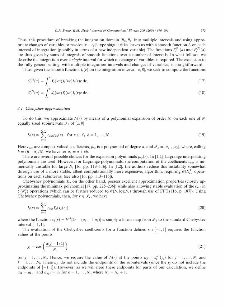
O.P. Bruno, E.M. Hyde / Journal of Computational Physics 200 (2004) 670–694 675
Thus, this procedure of breaking the integration domain ½R0;R1� into multiple intervals and using appro-
priate changes of variables to resolve jr � r0jc-type singularities leaves us with a smooth function I‘ on each
interval of integration (possibly in terms of a new independent variable). The functions F ð1Þ‘ ðaÞ and F ð2Þ
‘ ðaÞare thus given by sums of integrals of smooth functions over a number of intervals. In what follows, we
describe the integration over a single interval for which no change of variables is required. The extension to
the fully general setting, with multiple integration intervals and changes of variables, is straightforward.
Thus, given the smooth function I‘ðrÞ on the integration interval ½a; b�, we seek to compute the functions
Gð1Þ‘ ðaÞ ¼
Z a
aY‘ðjaÞJ‘ðjrÞI‘ðrÞr dr; ð17Þ
Gð2Þ‘ ðaÞ ¼
Z b
aJ‘ðjaÞY‘ðjrÞI‘ðrÞr dr: ð18Þ
3.1. Chebyshev approximation
To do this, we approximate I‘ðrÞ by means of a polynomial expansion of order Nc on each one of Ni
equally sized subintervals Ik of ½a; b�
I‘ðrÞ �XNc�1
n¼0
cnk‘pnkðrÞ for r 2 Ik; k ¼ 1; . . . ;Ni: ð19Þ
Here cnk‘ are complex-valued coefficients, pnk is a polynomial of degree n, and Ik ¼ ½ak�1; ak�, where, callingh ¼ ðb� aÞ=Ni, we have set ak ¼ aþ kh.
There are several possible choices for the expansion polynomials pnkðrÞ. In [1,2], Lagrange interpolating
polynomials are used. However, for Lagrange polynomials, the computation of the coefficients cnk‘ is nu-merically unstable for large Nc [16, pp. 113–116]. In [1,2], the authors reduce this instability somewhat
through use of a more stable, albeit computationally more expensive, algorithm, requiring OðN 3c Þ opera-
tions on each subinterval (see also [16, pp. 113–116]).
Chebyshev polynomials Tn, on the other hand, possess excellent approximation properties (closely ap-
proximating the minimax polynomial [17, pp. 225–236]) while also allowing stable evaluation of the cnk‘ inOðN 2
c Þ operations (which can be further reduced to OðNc logNcÞ through use of FFTs [16, p. 187]). Using
Chebyshev polynomials, then, for r 2 Ik, we have
I‘ðrÞ �XNc�1
n¼0
cnk‘Tn xkðrÞð Þ; ð20Þ
where the function xkðrÞ ¼ h�1½2r � ðak�1 þ akÞ� is simply a linear map from Ik to the standard Chebyshev
interval ½�1; 1�.The evaluation of the Chebyshev coefficients for a function defined on ½�1; 1� requires the function
values at the points
yj ¼ cospðj� 1=2Þ
Nc
� �ð21Þ
for j ¼ 1; . . . ;Nc. Hence, we require the value of I‘ðrÞ at the points ajk ¼ x�1k ðyjÞ for j ¼ 1; . . . ;Nc and
k ¼ 1; . . . ;Ni. These ajk do not include the endpoints of the subintervals (since the yj do not include the
endpoints of ½�1; 1�). However, as we will need these endpoints for parts of our calculation, we define
a0k ¼ ak�1 and aNpk ¼ ak for k ¼ 1; . . . ;Ni, where Np ¼ Nc þ 1.
676 O.P. Bruno, E.M. Hyde / Journal of Computational Physics 200 (2004) 670–694
Since in our algorithm the order Np of the Chebyshev approximation is held fixed, evaluation of the
coefficients cnkl for n ¼ 0; . . . ;Nc � 1, k ¼ 1; . . . ;Ni and ‘ ¼ �M ; . . . ;M requires a total of
OðNpNiMÞ ¼ OðNÞmemory and OðNiMN 2p Þ ¼ OðNÞ operations. As noted earlier, the N 2
p complexity requiredby the Chebyshev approximation could be reduced to OðNp logNpÞ by use of FFTs. Note that, since Np
remains fixed, however, a recourse to FFTs does not improve the overall asymptotic complexity. And, more
importantly, since we typically use a relatively small value of Np, e.g., Np ¼ 9; 17, we have found that use of
FFTs in this context provides little additional benefit.
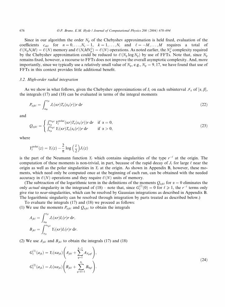
3.2. High-order radial integration
As we show in what follows, given the Chebyshev approximations of I‘ on each subinterval Ik of ½a; b�,the integrals (17) and (18) can be evaluated in terms of the integral moments
Pnjk‘ ¼Z ajk
a0k
J‘ðjrÞTn xkðrÞð Þr dr ð22Þ
and
Qnjk‘ ¼R aNpkajk
Y polar‘ ðjrÞTn xkðrÞð Þr dr if a ¼ 0;R aNpk
ajkY‘ðjrÞTn xkðrÞð Þr dr if a > 0;
(ð23Þ
where
Y polar‘ ðzÞ ¼ Y‘ðzÞ �
2
plog
z2
� �J‘ðzÞ
is the part of the Neumann function Y‘ which contains singularities of the type r�‘ at the origin. The
computation of these moments is non-trivial, in part, because of the rapid decay of J‘ for large ‘ near theorigin as well as the polar singularities in Y‘ at the origin. As shown in Appendix B, however, these mo-ments, which need only be computed once at the beginning of each run, can be obtained with the needed
accuracy in OðNÞ operations and they require OðNÞ units of memory.
(The subtraction of the logarithmic term in the definitions of the moments Qnjk‘ for a ¼ 0 eliminates the
only actual singularity in the integrand of (18) – note that, since Gð2Þ‘ ð0Þ ¼ 0 for ‘P 1, the r�‘ terms only
give rise to near-singularities, which can be resolved by Gaussian integrations as described in Appendix B.
The logarithmic singularity can be resolved through integration by parts treated as described below.)
To evaluate the integrals (17) and (18) we proceed as follows:
(1) We use the moments Pnjk‘ and Qnjk‘ to obtain the integrals
Ajk‘ ¼Z ajk
a0k
J‘ðjrÞI‘ðrÞr dr;
Bjk‘ ¼Z aNpk
ajk
Y‘ðjrÞI‘ðrÞr dr:
(2) We use Ajk‘ and Bjk‘ to obtain the integrals (17) and (18)
Gð1Þ‘ ðajkÞ ¼ Y‘ðjajkÞ Ajk‘
þXk�1
q¼1
ANpq‘
!;
Gð2Þ‘ ðajkÞ ¼ J‘ðjajkÞ Bjk‘
þXNi
q¼kþ1
B0q‘
!:
ð24Þ

O.P. Bruno, E.M. Hyde / Journal of Computational Physics 200 (2004) 670–694 677
Remark 3. The quantities Ajk‘ can be obtained directly from the Pnjk‘:
Ajk‘ � Y‘ðjajkÞXNc�1
n¼0
cnk‘Pnjk‘:
Similarly, for a > 0, the Bjk‘ are obtained directly from the Qnjk‘:
Bjk‘ � J‘ðjajkÞXNc�1
n¼0
cnk‘Qnjk‘:
Our method for the evaluation of Gð2Þ‘ ðajkÞ in the case a ¼ 0, which is less direct, is described below.
Remark 4. In practice, for large values of ‘, the function J‘ (resp. Y‘) may underflow (resp. overflow)causing the quantities Ajk‘ (resp. Bjk‘) in point (1) above, in turn, to underflow (resp. overflow). To over-
come this difficulty, for sufficiently large values of the ratio ‘=ðjajkÞ, we redefine Ajk‘, Bjk‘, Pnjk‘ and Qnjk‘,
e.g.,
Ajk‘ ¼Z ajk
a0k
Y‘ðjajkÞJ‘ðjrÞI‘ðrÞr dr;
Pnjk‘ ¼Z ajk
a0k
Y‘ðjajkÞJ‘ðjrÞTn xkðrÞð Þr dr;ð25Þ
with analogous redefinitions of Bjk‘ and Qnjk‘, and corresponding changes to (24). It is easy to check that, in
view of the asymptotic properties of J‘ and Y‘, the quantities (25) do not underflow or overflow. A method
for the evaluation of products of the form J‘ðz1ÞY‘ðz2Þ that are needed in (25) is presented in Section 4.
As mentioned in Remark 3, it remains for us to evaluate Gð2Þ‘ ðajkÞ in the case a ¼ 0. In view of the
relation
Bjk‘ �Z aNpk
ajk
2
plog
jr2
� �J‘ðjrÞI‘ðrÞr dr þ
XNc�1
n¼0
cnk‘Qnjk‘;
to do this it suffices to evaluate integrals of the formZ b
a
2
plog
jr2
� �J‘ðjrÞI‘ðrÞr dr ð26Þ
for all relevant values of ‘ and a 2 ½a; b� ¼ ½0; b�.To evaluate the integrals (26), we integrate the logarithmic term by parts to obtainZ b
alog
jr2
� �J‘ðjrÞI‘ðrÞr dr ¼ log
jr2
� �Z r
0
J‘ðjqÞI‘ðqÞq dq
����ba
�Z b
adr
1
r
Z r
0
J‘ðjqÞI‘ðqÞq dq
¼ logjb2
� �Gð1Þ
‘ ðbÞ � logja2
� �Gð1Þ
‘ ðaÞ �Z b
ar�1Gð1Þ
‘ ðrÞ dr: ð27Þ
Since r�1Gð1Þ‘ ðrÞ is smooth for rP 0 (Gð1Þ
‘ ðrÞ ¼ OðrÞ as r ! 0), the last term in (27) can be computed by
means of the high-order Chebyshev approximation
r�1Gð1Þ‘ ðrÞ �
XNc�1
n¼0
dnk‘Tn xkðrÞð Þ for r 2 Ik:
The evaluation of the coefficients dnk‘ requires the values of Gð1Þ‘ ðajkÞ, which have been obtained previously.

678 O.P. Bruno, E.M. Hyde / Journal of Computational Physics 200 (2004) 670–694
As is known, the Chebyshev coefficients of an indefinite integral can be obtained easily from the coef-
ficients of the integrand [16, pp. 189, 190]; in our case, the Chebyshev coefficients Dnk‘ of the antiderivative
of r�1Gð1Þ‘ ðrÞ dr are given by
Dnk‘ ¼dn�1k‘ � dnþ1k‘
2n; nP 1:
The constant of integration D0k‘ is arbitrary. Clearly, this mapping requires only OðNÞ operations.In summary, given accurate values of the integral moments Pnjk‘ and Qnjk‘, the Chebyshev-based radial
integration method presented in this section evaluates the integrals (8) with high-order accuracy in OðNÞoperations. This algorithm is significantly more efficient and stable than the Lagrange polynomial approach
used in [1,2].
4. Accurate and efficient computation of scaled Bessel functions
As explained in Section 3, the rapid decay of the Bessel functions J‘ðzÞ and the rapid growth of the
Neumann functions Y‘ðzÞ as ‘ increases gives rise to quantities that underflow and overflow, respectively,
but whose product is machine-representable. To address these and other related issues we introduce certain
scaled versions of J‘ and Y‘.Noting that the leading order asymptotics of the functions J‘ðzÞ and Y‘ðzÞ near the origin are given by
J‘ðzÞ �1
‘!
z2
� �‘; ð28Þ
Y‘ðzÞ � � ð‘� 1Þ!p
z2
� ��‘
ð29Þ
for integers ‘ > 0 we introduce the scaled Bessel functions
~J‘ðzÞ ¼ ‘!z2
� ��‘
J‘ðzÞ; ð30Þ
~Y‘ðzÞ ¼ � pð‘� 1Þ!
z2
� �‘Y‘ðzÞ: ð31Þ
These scaled Bessel functions can be used to compute needed products and quotients of J‘ and Y‘. Forexample, we can compute the product J‘ðz1ÞY‘ðz2Þ for integers ‘ > 0 as
J‘ðz1ÞY‘ðz2Þ ¼ � 1
p‘z1z2
� �‘
~J‘ðz1Þ~Y‘ðz2Þ: ð32Þ
These scaled Bessel functions can be evaluated by recurrence-relation techniques similar to those used to
compute the conventional Bessel functions [16, pp. 173–175]. Indeed, from (30) and (31), and using the
recurrence relations for J‘ and Y‘, we obtain the recurrence relations
~J‘þ1ðzÞ ¼ ‘ð‘þ 1Þ 2
z
� �2
~J‘ðzÞh
� ~J‘�1ðzÞi; ð33Þ
~Y‘þ1ðzÞ ¼ ~Y‘ðzÞ �1
‘ð‘þ 1Þz2
� �2~Y‘�1: ð34Þ
O.P. Bruno, E.M. Hyde / Journal of Computational Physics 200 (2004) 670–694 679
Numerical experiments clearly demonstrate that, as is the case for the recurrence relation associated with
J‘ðzÞ and Y‘ðzÞ, for increasing ‘ the recurrence for ~J‘ is unstable and the recurrence for ~Y‘ is stable. Our
procedure for evaluation of the scaled Bessel functions thus proceeds as follows: we first use the classicalalgorithms to compute Y0ðzÞ and Y1ðzÞ, we scale these values, and we then use the recurrence relation (34) to
compute ~Y‘ðzÞ. To compute ~J‘ðzÞ, we use a downward recurrence and the normalization sum
1 ¼ J0ðzÞ þ 2X1n¼1
J2nðzÞ:
The implementation of this algorithm involves only relatively simple modifications to an existing recursive
algorithm for evaluation of the Bessel functions J‘ðzÞ or Y‘ðzÞ. In our codes, we used modified versions of
the Fortran77 routines rjbesl and rybesl, provided in the Netlib repository [18].
5. Efficient preconditioning
Sections 2 and 3 describe our integration method for the evaluation of the function KMvM for a given
function
vMða;/Þ ¼XM‘¼�M
v‘ðaÞei‘/:
For a given inhomogeneity and a given discretization, that method can be used to produce matrix–vector
products for the matrix associated with the linear system
v‘ðajkÞ � ðK‘vMÞðajkÞ ¼ ui‘ðajkÞ; ‘ ¼ �M ; . . . ;M ; ð35Þ
see Eq. (5). Clearly, this matrix–vector multiplication algorithm can be combined with any suitable iterative
linear solver to yield a fast, high-order solver for our scattering problem. For the non-Hermitian linear
systems arising in our context one may, in principle, use solvers such as GMRES, CGS, BiCGSTAB and
QMR [19]. We have found, however, that only GMRES and BiCGSTAB performed consistently well for
our problem; see e.g. [19] for a discussion of convergence rates of iterative linear solvers.
As is known, for a finite-dimensional linear system arising from discretization of a second-kind integral
equation, the number of iterations required by an iterative solver to obtain a given residual tolerance does
not depend on the mesh size. The number of iterations needed to meet a given tolerance does dependmarkedly on the size of the scatterer, however: for a given scattering geometry, as the frequency and/or the
values of m are increased, the number of iterations required to achieve a given residual tolerance can in-
crease considerably.
In this section, we introduce a preconditioning method which, based on use of approximate scatterers
and associated preconditioning matrices P , can reduce significantly the number of iterations required by
iterative solvers in our context. To construct a preconditioner we begin by approximating a given inho-
mogeneity m by a piecewise-constant, radially layered inhomogeneity em; a preconditioner is then obtained
as the inverse of an integral operator associated with em which, using a certain differential equation togetherwith radial integration methods similar to those described in the previous sections, can be applied in OðNÞoperations. (The solution to this preconditioning integral operator bears some similarities to the well-
known Mie series solution for scattering by a piecewise-constant layered cylinder; see Remark 5 for more
details.)
To complete our preconditioning prescriptions we must make appropriate choices of the approximating
inhomogeneities em. In Section 5.2 we determine an approximating scatterer em for a given scatterer m which,
680 O.P. Bruno, E.M. Hyde / Journal of Computational Physics 200 (2004) 670–694
according to our extensive numerical experiments, is optimal: for a large class of scattering obstacles, in-
cluding all of the test cases considered in Section 6, the em functions introduced in Section 6 provide the
sharpest decreases in iteration numbers amongst those arising from admissible approximating scatterers.
5.1. Evaluation of the preconditioning operator
As mentioned above, we use functions em of the form
emðxÞ ¼Xqj¼1
mjvAjðxÞ;
where mj are constants, vAjis the characteristic function of the set Aj, and where Aj (j ¼ 1; 2; . . . ; q) denote
the annular sets
Aj ¼ fx : aj�1 6 jxj6 ajg; 0 ¼ a0 < a1 < � � � < aq ¼ R1:
Here we have assumed that R0 ¼ 0 for definiteness; the case for R0 > 0 can be treated similarly – the slight
departures in treatment that occur in this case will be pointed out at appropriate points in the text. The
preconditioner P we use equals the inverse of the matrix associated with the integral equation
mðxÞ þ j2Xqj¼1
mj
ZAj
Uðjjx� yjÞmðyÞ dy ¼ xðxÞ; ð36Þ
where, for convenience, the Green function g is expressed explicitly in terms of the Hankel functionUðzÞ ¼ ði=4ÞH 1
0 ðzÞ. Given the inverse operator P , our left-preconditioned equation reads
P ðI � KMÞvM ¼ Pui;M :
This new, preconditioned linear system is solved using an iterative solver, as described previously. In detail,
after evaluating the right-hand side vector Pui;M by solving Eq. (36) with x ¼ ui;M , at each iteration of the
linear solver, we solve (36) with x ¼ ðI � KMÞvM for the function vM produced by the previous iteration of
the iterative solver. Note that in both cases we have x ¼ xM .
To solve Eq. (36) for a given right-hand side x we derive a differential equation for the new unknownl ¼ m� x, where m is the solution of Eq. (36). Although m is only defined for jxj6R1, we can extend l to all
of R2 by
lðxÞ ¼ �j2Xqj¼1
mj
ZAj
Uðjjx� yjÞmðyÞ dy:
Clearly, for x 2 Aj, we have
ðDþ j2n2j ÞlðxÞ ¼ j2mjx; j ¼ 1; 2; . . . ; q; ð37Þ
where mj ¼ 1� n2j and for jxj > R1 (and jxj < R0 when R0 6¼ 0), we have
ðDþ j2ÞlðxÞ ¼ 0: ð38Þ
Further, l 2 C1ðR2Þ [20, pp. 53, 56] and, as it is easily seen, l satisfies the Sommerfeld radiation condition
as jxj ! 1 [7, pp. 216–217]. Thus, Eqs. (37) and (38) together with the Sommerfeld radiation condition and
conditions of continuity of the function l and its radial derivatives at jxj ¼ aj (j ¼ 0; . . . ; q) make up a
differential equation for l in all of R2 that is equivalent to the preconditioning integral equation (36).
O.P. Bruno, E.M. Hyde / Journal of Computational Physics 200 (2004) 670–694 681
To solve this differential equation we express the solution as a sum of a particular solution and a solution
of the associated homogeneous problem, lðxÞ ¼ lpðxÞ þ lhðxÞ. For x 2 Aj, a particular solution to the
equation is given by
lpðxÞ ¼ �j2mj
ZAj
Uðjnjjx� yjÞxðyÞ dy:
Since x ¼ xM , it follows that lp ¼ lMp and, further, in polar coordinates ða;/Þ, we have
ðlpÞ‘ðaÞ ¼ �j2mj H 1‘ ðjnjaÞ
Z a
aj�1
J‘ðjnjrÞx‘ðrÞr dr"
þ J‘ðjnjaÞZ aj
aH 1
‘ ðjnjrÞx‘ðrÞr dr#
ð39Þ
for aj�1 6 a6 aj. Clearly, these integrals can be computed with high-order accuracy and in OðNÞ operationsusing the radial integration method introduced in Section 3. Since this integration algorithm requires thevalues of x‘ðrÞ at Chebyshev points, we choose the preconditioning intervals ½aj�1; aj� to correspond to the
radial integration intervals used to compute xM ¼ ðI � KMÞvM , so that interpolations are not needed to
obtain the required values of x‘ðrÞ.The solution of the homogeneous problem, on the other hand, can be expressed in the form
lhða;/Þ ¼P1
‘¼�1 að1Þ‘ J‘ðjnjaÞei‘/ if j ¼ 1;P1‘¼�1 aðjÞ‘ J‘ðjnjaÞ þ bðj�1Þ
‘ Y‘ðjnjaÞh i
ei‘/ if j ¼ 2; 3; . . . ; q
(ð40Þ
for aj�1 6 a6 aj. (If R0 > 0, the solution of the homogeneous problem for j ¼ 1 is given by a linear com-
bination of J‘ and Y‘ instead of J‘ alone. Furthermore, if R0 > 0, we must consider the solution of the
homogeneous problem in the additional region a < R0, which takes the same form as for j ¼ 1 in (40).)
Finally, for a > R1, we have
lða;/Þ ¼X1‘¼�1
bðqÞ‘ H 1
‘ ðjaÞei‘/:
Clearly, given the correct values of the coefficients aðjÞ‘ and bðjÞ‘ , we can compute ðlhÞ‘ðaÞ for ‘ ¼ �M ; . . . ;M
and all radial discretization points in OðNÞ operations.
Remark 5. Our preconditioner is related to the Mie series solution of (1) for a layered cylinder with a
piecewise-constant refractive index. Indeed, the form of the solution lh of the homogeneous problem ex-
actly matches that of the Mie series solution. However, unlike the Mie solution, the inhomogeneous
equation (37) requires a particular solution lp in addition to lh, which, in turn, affects the coefficients in the
series expansion of lh through the continuity conditions on the boundaries between the annular regions.
Equations determining the values of the 2q coefficients aðjÞ‘ and bðjÞ‘ are obtained by enforcing the con-
ditions mentioned above, of continuity of l and its radial derivatives at the points aj, j ¼ 1; 2; . . . ; q. Forj ¼ 2; 3; . . . ; q� 1, we have
aðjÞ‘ J‘ðjnjajÞ þ bðj�1Þ‘ Y‘ðjnjajÞ þ ðlpÞ‘ða�j Þ ¼ aðjþ1Þ
‘ J‘ðjnjþ1ajÞ þ bðjÞ‘ Y‘ðjnjþ1ajÞ þ ðlpÞ‘ðaþj Þ
and
aðjÞ‘ njJ 0‘ðjnjajÞ þ bðj�1Þ
‘ njY 0‘ ðjnjajÞ þ
1
jðlpÞ
0‘ða�j Þ
¼ aðjþ1Þ‘ njþ1J 0
‘ðjnjþ1ajÞ þ bðjÞ‘ njþ1Y 0
‘ ðjnjþ1ajÞ þ1
jðlpÞ
0‘ðaþj Þ:
682 O.P. Bruno, E.M. Hyde / Journal of Computational Physics 200 (2004) 670–694
Here ðlpÞ‘ðaþj Þ ¼ lima!aþjðlpÞ‘ðaÞ and ðlpÞ‘ða�j Þ ¼ lima!a�j
ðlpÞ‘ðaÞ with corresponding definitions for the
derivatives. The equations for j ¼ 1 and j ¼ q are similar.
For each ‘, the matrix associated with this linear system is constant and banded with five diagonals.Hence, we compute the LU -decomposition of all of these matrices in OðqMÞ operations [21, pp. 152, 153]only once at the beginning of each run. In each iteration, after computing the ðlpÞ‘ðaþj Þ and ðlpÞ‘ða�j Þ andtheir derivatives, we use the LU -decomposition to solve for the values of aðjÞ‘ and bðjÞ
‘ for all j ¼ 1; 2; . . . ; q.This again requires a total of OðqMÞ operations [21, pp. 152, 153].
Finally, we compute ðlpÞ‘ðaþj Þ and ðlpÞ‘ða�j Þ and their derivatives. By (39), we have
ðlpÞ‘ðaþj�1Þ ¼ � ip2j2mjJ‘ðjnjaj�1Þ
Z aj
aj�1
H 1‘ ðjnjrÞx‘ðrÞr dr;
ðlpÞ‘ða�j Þ ¼ � ip2j2mjH 1
‘ ðjnjajÞZ aj
aj�1
J‘ðjnjrÞx‘ðrÞr dr
and
ðlpÞ0‘ðaþj�1Þ ¼ � ip
2j3njmjJ 0
‘ðjnjaj�1ÞZ aj
aj�1
H 1‘ ðjnjrÞx‘ðrÞr dr;
ðlpÞ0‘ða�j Þ ¼ � ip
2j3njmjðH 1
‘ Þ0ðjnjajÞ
Z aj
aj�1
J‘ðjnjrÞx‘ðrÞr dr:
These integrals are easily obtained from the values of ðlpÞ‘ðaÞ in OðqMÞ operations.This completes the description of the preconditioner resulting from a given approximating inhomoge-
neity em; the constructions above show that such a preconditioner can be applied in just OðNÞ operations periteration. A discussion on selection of the function em is given in the following section.
5.2. Optimal choice of preconditioning parameters
Naturally, the effectiveness of the preconditioner in reducing iteration numbers depends on the choice of
the annuli Aj and the approximating indices mj. A rather extensive set of numerical experiments we have
conducted suggest the following strategy for the selection of these parameters: (1) use annuli Aj whoseboundaries are tangent to curves of discontinuity in the actual index m; (2) use values mj equal to the
average value of m on the outside boundary of each Aj.
Following these rules, the optimal preconditioning parameters for the scatterers in Section 6.2 are as
follows: (1) for the ‘‘bumpy’’ scatterer (Fig. 4) we use a single annulus A1 (actually a disc in this case)
covering the background disc and with m1 ¼ �3, the in-disc background index; (2) for the square-shaped
scatterer (Fig. 2) and the star-shaped scatterer (Fig. 3), we use two preconditioning annuli, A1 and A2: A1 is
the inscribed disc and m1 equals the value of m on that disc, which is a constant; the outer boundary of A2
circumscribes the scatterer and m2 ¼ 0.As demonstrated by the various tables in Section 6.2, with these prescriptions for the preconditioning
parameters, the preconditioner introduced in this section can lead to very significant decreases in iteration
numbers. The reductions that result from this preconditioner depend on the character of the given scat-
tering geometry. To analyze the performance of the preconditioner as the scatterer geometry changes, we
compared the number of iterations required to meet a given tolerance with and without preconditioning for
elliptical scatterers of varying eccentricity. We used elliptical scatterers with constant refractive index n ¼ 2
(m ¼ �3), major axis of length equal to 10 interior wavelengths, and various minor axes. In accordance
with our prescriptions above, the preconditioner contains two annuli, one inscribed with m1 ¼ �3 and onewhose outer boundary circumscribes the ellipse, with m2 ¼ 0. As we varied the length of the minor axis
0 1 2 3 4 5 6 7 8 9 100
50
100
150
200
250
300
350
400
Length of Minor Axis (Interior Wavelengths)
Num
ber
of G
MR
ES
Iter
atio
ns (
Tol
eran
ce =
1.e
8)
w/o P w/ P
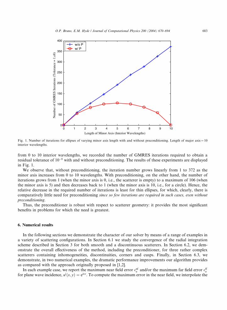
Fig. 1. Number of iterations for ellipses of varying minor axis length with and without preconditioning. Length of major axis¼ 10
interior wavelengths.
O.P. Bruno, E.M. Hyde / Journal of Computational Physics 200 (2004) 670–694 683
from 0 to 10 interior wavelengths, we recorded the number of GMRES iterations required to obtain a
residual tolerance of 10�8 with and without preconditioning. The results of these experiments are displayed
in Fig. 1.
We observe that, without preconditioning, the iteration number grows linearly from 1 to 372 as the
minor axis increases from 0 to 10 wavelengths. With preconditioning, on the other hand, the number of
iterations grows from 1 (when the minor axis is 0, i.e., the scatterer is empty) to a maximum of 106 (whenthe minor axis is 5) and then decreases back to 1 (when the minor axis is 10, i.e., for a circle). Hence, the
relative decrease in the required number of iterations is least for thin ellipses, for which, clearly, there is
comparatively little need for preconditioning since so few iterations are required in such cases, even without
preconditioning.
Thus, the preconditioner is robust with respect to scatterer geometry: it provides the most significant
benefits in problems for which the need is greatest.
6. Numerical results
In the following sections we demonstrate the character of our solver by means of a range of examples in
a variety of scattering configurations. In Section 6.1 we study the convergence of the radial integration
scheme described in Section 3 for both smooth and a discontinuous scatterers. In Section 6.2, we dem-
onstrate the overall effectiveness of the method, including the preconditioner, for three rather complex
scatterers containing inhomogeneities, discontinuities, corners and cusps. Finally, in Section 6.3, we
demonstrate, in two numerical examples, the dramatic performance improvements our algorithm providesas compared with the approach originally proposed in [1,2].
In each example case, we report the maximum near field error �nfu and/or the maximum far field error �ffufor plane wave incidence, uiðx; yÞ ¼ eijx. To compute the maximum error in the near field, we interpolate the
684 O.P. Bruno, E.M. Hyde / Journal of Computational Physics 200 (2004) 670–694
solution computed by our method to an evenly spaced polar grid. On this grid, we compute the maximum
absolute error as compared with either the analytical solution (when it is available) or the solution com-
puted with a finer discretization. The maximum error in the far field is computed similarly by interpolatingto an evenly spaced angular grid. The results for each example are given in the accompanying figures and
tables. These results were obtained using the GMRES iterative solver on a 1.7 GHz Pentium Xeon.
6.1. Convergence of the radial integration algorithm
In this section, we demonstrate the high-order convergence of the radial integration method described
in Section 3. (Of course, here and throughout the examples in this text we also make use of the scaled
Bessel function algorithm described in Section 4.) The degree of accuracy in the radial integration isdetermined by the number of subintervals Ni and the number Nc of Chebyshev points per subinterval used
to approximate I‘ðrÞ (see Appendix B for the parameters used in the evaluation of the integral moments
(22) and (23)).
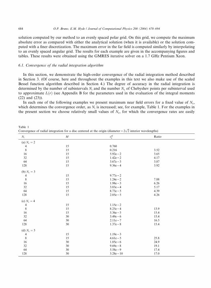
In each one of the following examples we present maximum near field errors for a fixed value of Nc,
which determines the convergence order, as Ni is increased; see, for example, Table 1. For the examples in
the present section we choose relatively small values of Nc, for which the convergence rates are easily
Table 1
Convergence of radial integration for a disc centered at the origin (diameter¼ 2ffiffiffi2
pinterior wavelengths)
Ni M �nfu Ratio
(a) Nc ¼ 2
4 15 0.760
8 15 0.216 3.52
16 15 5.92e) 2 3.65
32 15 1.42e) 2 4.17
64 15 3.67e) 3 3.87
128 15 9.36e) 4 3.92
(b) Nc ¼ 3
4 15 9.77e) 2
8 15 1.24e) 2 7.88
16 15 1.98e) 3 6.26
32 15 3.83e) 4 5.17
64 15 8.73e) 5 4.39
128 15 2.05e) 5 4.26
(c) Nc ¼ 4
4 15 1.15e) 2
8 15 8.25e) 4 13.9
16 15 5.36e) 5 15.4
32 30 3.49e) 6 15.4
64 30 2.11e) 7 16.5
128 30 1.37e) 8 15.4
(d) Nc ¼ 5
4 15 1.19e) 3
8 15 4.61e) 5 25.8
16 30 1.85e) 6 24.9
32 30 9.69e) 8 19.1
64 30 5.58e) 9 17.4
128 30 3.28e) 10 17.0

Table 2
Convergence of radial integration for a disc centered at ð1k; 0Þ (diameter¼ffiffiffi2
pinterior wavelengths)
Ni M �nfu Ratio
(a) Nc ¼ 2 without change of variable
1 15 2.34
2 15 1.45 1.61
4 15 0.499 2.91
8 30 0.167 2.99
16 30 4.69e) 2 3.56
32 30 1.31e) 2 3.58
64 60 4.48e) 3 2.92
(b) Nc ¼ 2 with change of variable
1 15 2.93
2 15 1.92 1.53
4 15 0.668 2.87
8 15 0.204 3.27
16 30 5.51e) 2 3.70
32 30 1.53e) 2 3.60
64 60 3.78e) 3 4.05
(c) Nc ¼ 4 without change of variable
1 7 1.52
2 15 0.159 9.56
4 30 2.09e) 2 7.61
8 60 6.91e) 3 3.02
16 60 2.44e) 3 2.83
32 120 5.88e) 4 4.15
64 120 3.17e) 4 1.85
(d) Nc ¼ 4 with change of variable
1 15 1.82
2 15 0.748 2.43
4 30 3.69e) 2 20.27
8 60 3.25e) 3 11.35
16 120 4.06e) 4 8.00
32 480 2.28e) 5 17.81
64 480 6.98e) 6 3.27
(e) Nc ¼ 8 without change of variable
1 30 2.60e) 2
2 30 6.82e) 3 3.81
4 60 2.39e) 3 2.85
8 120 7.01e) 4 3.41
16 120 3.11e) 4 2.25
32 240 1.14e) 4 2.73
64 480 2.41e) 5 4.73
(f) Nc ¼ 8 with change of variable
1 15 0.536
2 30 1.17e) 2 45.81
4 60 1.23e) 3 9.51
8 240 1.78e) 4 6.91
16 480 4.61e) 5 3.86
32 960 3.86e) 6 11.94
64 1920 3.40e) 7 11.35
O.P. Bruno, E.M. Hyde / Journal of Computational Physics 200 (2004) 670–694 685

686 O.P. Bruno, E.M. Hyde / Journal of Computational Physics 200 (2004) 670–694
observed. In practice (in the following sections), we use significantly larger values of Nc, which are much
more advantageous. In each table, we also report the number of modesM used in the calculation. To ensure
that the near field errors reported reflect the convergence rate of the radial integration scheme alone, inTables 1 and 2 sufficiently large values of M were used so that the angular integration error is smaller than
the radial integration error.
We demonstrate the radial convergence rates in two examples for which exact solutions are known: (1) a
disc with constant refractive index centered at the origin, and (2) a disc with constant refractive index
centered away from the origin. Although these scatterers are similar from a physical point of view, they
present significantly different degrees of difficulty to our numerical algorithm. In particular, the disc cen-
tered at the origin gives rise to a smooth (constant) refractive index function within the integration domain
whereas the disc centered away from the origin nðxÞ is discontinuous in the integration domain. As de-scribed previously, a discontinuous refractive index requires special treatment: (1) a change of variables is
required to resolve associated square-root singularities (see Section 3 and Appendix A), and (2) substitution
by a truncated Fourier series m2M is used (see Section 2).
In Table 1 we present results for the disc of diameter 2k centered at the origin with refractive index
n ¼ffiffiffi2
p, where k is the wavelength of the incident field. Since, as it is apparent from these results, our radial
integration method converges as N�Nc
i if Nc is even and as N�ðNc�1Þi if Nc is odd (a behavior similar to that
exhibited by the Newton–Cotes quadrature rules [17, p. 264]), in practice, we only use even values of Nc.
The value of Nc should be selected to balance convergence order and computational cost (the computationof the radial integrals requires OðN 2
cNiMÞ ¼ OðNcNÞ operations); in our experience, we have found that the
choice Nc ¼ 16 strikes this balance quite well.
Results for the disc centered at ð1k; 0Þ are given in Table 2. In this case, the disc has a diameter of 1k and
a refractive index of n ¼ffiffiffi2
p. We display the near and far field errors obtained with and without the change
of variables, which resolves the square-root singularities in I‘ðrÞ (see Appendix A). We only present results
for even values of Nc. We see that significant improvements in the convergence rate result when the change
of variables is used.
Remark 6. From Tables 1 and 2, we observe that the number of Fourier modesM required to obtain a high
degree of accuracy is much higher for the off-center disc than for the disc centered at the origin. (To obtain a
low degree of accuracy, only small values of M are required in both cases.) This is a direct consequence of
the fact, emphasized previously, that the index mðr; hÞ for the off-center disc is a discontinuous function on
the integration domain while the index for the disc centered at the origin is a C1 function on the integration
domain. This difference in regularity gives rise to the difference in convergence rates that, in turn, is related
to the differences in the values of M required for a given accuracy. As established in [13], the convergence
rate of the algorithm under consideration for a discontinuous scatterer is OðM�2Þ in the near field andOðM�3Þ in the far field. The convergence rate for a C1 scatterer, on the other hand, is superalgebraic in M .
Thus, we expect OðM�3Þ far field convergence for any discontinuous m; see, for example, the convergence
behavior for the square-shaped scatterer in Table 3.
6.2. Complex scatterers and preconditioning
In this section, we demonstrate the capabilities of our method and the performance of our precondi-
tioner by considering three rather complex scattering geometries. The first two of these scatterers containgeometric singularities, corners and cusps, respectively, as well as discontinuities in nðxÞ. The last example
contains smooth indentations and protrusions in a constant background, providing an example of a truly
inhomogeneous, smooth refractive index distribution. In each example, we present the maximum near and
far field errors as we increase Ni and M while fixing Nc ¼ 16. We choose the preconditioning parameters for
each scatterer as described in Section 5.2. Furthermore, we report the number of GMRES iterations as well
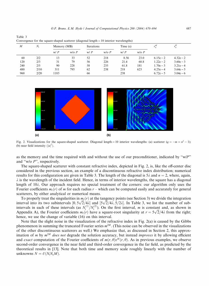
Fig. 2. Visualizations for the square-shaped scatterer. Diagonal length¼ 10 interior wavelengths: (a) scatterer (q ¼ �m ¼ n2 � 1);
(b) near field intensity ðjuj2Þ.
Table 3
Convergence for the square-shaped scatterer (diagonal length¼ 10 interior wavelengths)
M Ni Memory (MB) Iterations Time (s) �nfu �ffu
w/ P w/o P w/ P w/o P w/ P w/o P
60 2/2 13 33 52 218 8.56 23.0 6.15e) 2 4.32e) 2
120 2/3 31 79 56 226 21.4 60.8 1.22e) 2 3.60e) 3
240 2/5 90 228 58 235 61.8 181 1.70e) 3 3.21e) 4
480 2/10 311 795 62 238 218 623 4.25e) 4 3.64e) 5
960 2/20 1183 66 238 6.72e) 5 3.04e) 6
O.P. Bruno, E.M. Hyde / Journal of Computational Physics 200 (2004) 670–694 687
as the memory and the time required with and without the use of our preconditioner, indicated by ‘‘w/P ’’and ‘‘w/o P ’’, respectively.
The square-shaped scatterer with constant refractive index, depicted in Fig. 2, is, like the off-center disc
considered in the previous section, an example of a discontinuous refractive index distribution; numerical
results for this configuration are given in Table 3. The length of the diagonal is 5k and n ¼ 2, where, again,
k is the wavelength of the incident field. Hence, in terms of interior wavelengths, the square has a diagonal
length of 10k. Our approach requires no special treatment of the corners: our algorithm only uses theFourier coefficients m‘ðrÞ of m for each radius r – which can be computed easily and accurately for general
scatterers, by either analytical or numerical means.
To properly treat the singularities in m‘ðrÞ at the tangency points (see Section 3) we divide the integration
interval into its two subintervals ½0; 5ffiffiffi2
p=4k� and ½5
ffiffiffi2
p=4k; 5=2k�. In Table 3, we list the number of sub-
intervals in each of these intervals (as N ð1Þi =N ð2Þ
i ). On the first interval, m is constant and, as shown in
Appendix A), the Fourier coefficients m‘ðrÞ have a square-root singularity at r ¼ 5ffiffiffi2
p=4k from the right;
hence, we use the change of variable (16) on this interval.
Note that the slight noise in the visualization of the refractive index in Fig. 2(a) is caused by the Gibbsphenomenon in summing the truncated Fourier series m2M . (This noise can be observed in the visualizations
of the other discontinuous scatterers as well.) We emphasize that, as discussed in Section 2, this approx-
imation of m by m2M does not degrade the solution accuracy, but instead improves it by allowing efficient
and exact computation of the Fourier coefficients of mðr; hÞvMðr; hÞ. As in previous examples, we observe
second-order convergence in the near field and third-order convergence in the far field, as predicted by the
theoretical results in [13]. Note that both time and memory scale roughly linearly with the number of
unknowns N ¼ OðNiNcMÞ.
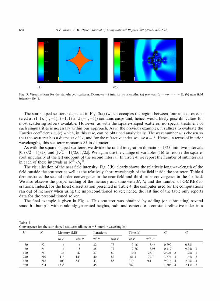
Fig. 3. Visualizations for the star-shaped scatterer. Diameter¼ 8 interior wavelengths: (a) scatterer (q ¼ �m ¼ n2 � 1); (b) near field
intensity ðjuj2Þ.
688 O.P. Bruno, E.M. Hyde / Journal of Computational Physics 200 (2004) 670–694
The star-shaped scatterer depicted in Fig. 3(a) (which occupies the region between four unit discs cen-tered at ð1; 1Þ, ð1;�1Þ, ð�1; 1Þ and ð�1;�1Þ) contains cusps and, hence, would likely pose difficulties for
most scattering solvers available. However, as with the square-shaped scatterer, no special treatment of
such singularities is necessary within our approach. As in the previous examples, it suffices to evaluate the
Fourier coefficients m‘ðrÞ which, in this case, can be obtained analytically. The wavenumber j is chosen so
that the scatterer has a diameter of 1k, and for the refractive index we use n ¼ 8. Hence, in terms of interior
wavelengths, this scatterer measures 8k in diameter.
As with the square-shaped scatterer, we divide the radial integration domain ½0; 1=2k� into two intervals
½0; ðffiffiffi2
p� 1Þ=2k� and ½ð
ffiffiffi2
p� 1Þ=2k; 1=2k�. We again use the change of variables (16) to resolve the square-
root singularity at the left endpoint of the second interval. In Table 4, we report the number of subintervals
in each of these intervals as N ð1Þi =N ð2Þ
i .
The visualization of the near field intensity, Fig. 3(b), clearly shows the relatively long wavelength of the
field outside the scatterer as well as the relatively short wavelength of the field inside the scatterer. Table 4
demonstrates the second-order convergence in the near field and third-order convergence in the far field.
We also observe the proper scaling of the memory and time with M , Ni and the number of GMRES it-
erations. Indeed, for the finest discretization presented in Table 4, the computer used for the computations
ran out of memory when using the unpreconditioned solver; hence, the last line of the table only reportsdata for the preconditioned solver.
The final example is given in Fig. 4. This scatterer was obtained by adding (or subtracting) several
smooth ‘‘bumps’’ with randomly generated heights, radii and centers to a constant refractive index in a
Table 4
Convergence for the star-shaped scatterer (diameter¼ 8 interior wavelengths)
M Ni Memory (MB) Iterations Time (s) �nfu �ffu
w/ P w/o P w/ P w/o P w/ P w/o P
30 1/2 6 6 32 73 3.16 3.46 0.792 0.581
60 1/4 14 15 35 77 7.76 8.95 0.112 9.34e) 2
120 1/6 36 42 37 80 19.5 23.7 2.02e) 2 1.28e) 2
240 1/10 113 143 40 82 61.3 72.7 3.87e) 3 1.65e) 3
480 1/18 403 543 43 85 219 261 9.01e) 4 2.06e) 4
960 1/34 1538 45 882 1.50e) 4 2.13e) 5
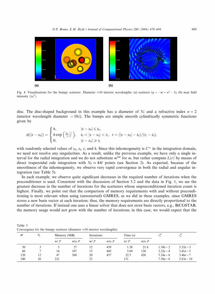
Fig. 4. Visualizations for the bumpy scatterer. Diameter �10 interior wavelengths: (a) scatterer (q ¼ �m ¼ n2 � 1); (b) near field
intensity ðjuj2Þ.
O.P. Bruno, E.M. Hyde / Journal of Computational Physics 200 (2004) 670–694 689
disc. The disc-shaped background in this example has a diameter of 5k and a refractive index n ¼ 2
(interior wavelength diameter ¼ 10k). The bumps are simple smooth cylindrically symmetric functionsgiven by
/ðjx� x0jÞ ¼h; jx� x0j6 t0;
h exp 2e�1=t
t�1
� �; t0 < jx� x0j < t1; t ¼ ðjx� x0j � t0Þ=ðt1 � t0Þ;
0; jx� x0jP t1
8><>:with randomly selected values of x0, t0, t1 and h. Since this inhomogeneity is C1 in the integration domain,
we need not resolve any singularities. As a result, unlike the previous example, we have only a single in-
terval for the radial integration and we do not substitute m2M for m, but rather compute I‘ðrÞ by means of
direct trapezoidal rule integration with Nh � 4M points (see Section 2). As expected, because of the
smoothness of the inhomogeneity, we observe very rapid convergence in both the radial and angular in-
tegration (see Table 5).
In each example, we observe quite significant decreases in the required number of iterations when the
preconditioner is used. Consistent with the discussion of Section 5.2 and the data in Fig. 1, we see thegreatest decrease in the number of iterations for the scatterers whose unpreconditioned iteration count is
highest. Finally, we point out that the comparison of memory requirements with and without precondi-
tioning is most relevant when using (unrestarted) GMRES, as we did in these examples, since GMRES
stores a new basis vector at each iteration; thus, the memory requirements are directly proportional to the
number of iterations. If instead one uses a linear solver that does not store basis vectors, e.g., BiCGSTAB,
the memory usage would not grow with the number of iterations; in this case, we would expect that the
Table 5
Convergence for the bumpy scatterer (diameter �10 interior wavelengths)
M Ni Memory (MB) Iterations Time (s) �nfu �ffu
w/ P w/o P w/ P w/o P w/ P w/o P
30 3 5 27 12 439 1.38 21.6 1.38e) 2 5.32e) 3
60 7 14 107 15 445 5.69 120 2.22e) 4 3.41e) 5
120 12 47 368 20 457 22.5 426 5.24e) 6 3.46e) 7
240 26 221 23 131 7.50e) 8 2.83e) 10

690 O.P. Bruno, E.M. Hyde / Journal of Computational Physics 200 (2004) 670–694
memory with preconditioning to somewhat exceed the memory without preconditioning because of the
storage requirements of the preconditioner itself.
6.3. Comparison with the original algorithm [1,2]
To compare the performance of the present method with that of the original algorithm [1,2] we
consider two main examples. First, we compare the performance of our algorithm with that of the
previous approach in a problem of scattering by a large disc with constant refractive index (compare
Fig. 1 of [2]). Here we evaluate the maximum far field error for a disc centered at the origin with n ¼ffiffiffi2
p
for jR ¼ 8 and jR ¼ 256. The plotted curves in Fig. 5 are obtained by holding the number of subin-
tervals Ni fixed (each value of Ni corresponds to one curve) and varying the degree d ¼ Np � 1 of theChebyshev polynomials.
For jR � 10� 15, we observe very similar results for the two approaches; compare, for example,
Fig. 5(a) below for jR ¼ 8 with the corresponding plot in Fig. 1 of [2]. However, the range jR � 10� 15
contains, roughly, the largest cylinders that the original approach could treat, owing to various inaccuracies
and instabilities (e.g., inaccuracies in the moments calculations [see Appendix B], underflow/overflow errors
in Bessel functions evaluations, etc.) as well as the lack of a preconditioner like the one we introduced in this
text. The present algorithm, on the other hand, still delivers significant accuracy for jR ¼ 256, which is of
the order of a 20 times larger (400 times larger in square wavelengths) than the largest problems that couldbe solved by means of the previous algorithm; see Fig. 5(b).
In our second example, we compare our algorithm’s performance with that of the previous approach, as
reported in [2], for the following smooth inhomogeneous scatterer:
mðx; yÞ ¼ �0:15ð1� xÞ2e�½x2þðyþ1Þ2� þ 0:5x5
�� x3 � y5
�e�ðx2þy2Þ þ 1
60e�½ðxþ1Þ2þy2� ð41Þ
for x2 þ y2 6 p2 and mðx; yÞ ¼ 0 otherwise. In Table 6, we report maximum far field errors and compu-
tational times for both algorithms under an assumed incident field with j ¼ 9. (The results for theoriginal approach were obtained from Table XI of [2].) Our algorithm ran on a 1.7 GHz PC and the
original approach ran on a 400 MHz PC. Even taking into account the differences in computer hardware
and software, our algorithm obviously far outperforms the original approach. We obtain, for example,
an error of 8:9� 10�13 in 2:12s compared with an error of 1:1� 10�8 obtained in 88:91s by the original
approach.
10 15 20 25 30
10−15
10−10
10−5
100
d
Err
or
3264
5 10 15
10−15
10−10
10−5
100
d(a) (b)
Err
or
12481632
Fig. 5. Maximum far field errors for scattering by the disc r6R as the degree d ¼ Np � 1 of the Chebyshev polynomials is increased for
each of several values of Ni: (a) jR ¼ 8; (b) jR ¼ 256.
Table 6
Convergence for the smooth inhomogeneous scatterer (41) with jR ¼ 9p
M Nr Time (s) Error
(a) Current algorithm
28 27 0.10 8.9e) 2
32 34 0.20 1.2e) 3
34 51 0.32 8.7e) 5
36 51 0.37 5.2e) 6
38 68 0.56 2.4e) 7
40 85 0.82 8.2e) 9
45 153 2.12 8.9e) 13
(b) Original algorithm
26 21 0.75 1.2e) 1
32 41 2.16 1.8e) 3
35 81 5.05 1.1e) 4
38 161 13.88 6.7e) 6
39 321 32.23 4.1e) 7
41 641 88.91 1.1e) 8
O.P. Bruno, E.M. Hyde / Journal of Computational Physics 200 (2004) 670–694 691
Acknowledgements
Color visualizations generated with the VTK-based visualization tool Vizamrai, developed by Steven
Smith at the Center for Applied Scientific Computing (CASC), Lawrence Livermore National Laboratory.
Appendix A. Determination of the singularities in m‘ðrÞ
As mentioned in Section 3, a point r ¼ r0 of tangency between polar circles and a discontinuity surface
oD gives rise to a jr � r0jc singularity in the functions m‘ðrÞ and I‘ðrÞ, for some c with 0 < c < 1. These
singularities must be resolved if high-order convergence in the radial integration algorithm is to be ob-
tained. In particular, it is important to evaluate c for a given tangency configuration; this can be done
easily, as we show in what follows.
Consider the expression (A.1) for the Fourier coefficients m‘ðrÞ. For r near the tangency radius r0, thecontribution to the Fourier coefficients m‘ðrÞ due to the set D is given by
m‘ðrÞ ¼1
2p
Z a2ðrÞ
a1ðrÞmðr; hÞe�i‘h dh; ðA:1Þ
where the quantities a1ðrÞ and a2ðrÞ give the polar coordinate angles at which the circle of radius r intersectsoD. Thus clearly, since mðr; hÞ is smooth for a1ðrÞ6 h6 a2ðrÞ, the singularity in m‘ðrÞ is determined solely by
the singularities in the functions a2ðrÞ and a1ðrÞ at r ¼ r0. The singularity in these functions, in turn, is
determined by the nature of the tangency between the circle r ¼ r0 and oD: a second-order tangency (in
which the local behavior of oD relative to the circle r ¼ r0 is quadratic) gives rise to c ¼ 1=2 whereas an nthorder tangency gives rise to c ¼ 1=n.
It follows that the off-center disc as well as the square- and star-shaped scatterers considered in Section 6
exhibit singularities with c ¼ 1=2. (These singularities are resolved by the change of variables (16).) For
example, in the case of the off-center disc, we expect singularities of the type ½r � ðd � RÞ�1=2 and
½ðd þ RÞ � r�1=2 at the tangency points r ¼ d � R and r ¼ d þ R, respectively. Explicit integration shows that
the Fourier coefficients m‘ðrÞ for the off-center disc are given by
692 O.P. Bruno, E.M. Hyde / Journal of Computational Physics 200 (2004) 670–694
m‘ðrÞ ¼�maðrÞp if ‘ ¼ 0;
�m sinð‘aðrÞÞp‘ if ‘ 6¼ 0;
(ðA:2Þ
for d � R6 r6 d þ R, where a2ðrÞ ¼ �a1ðrÞ ¼ aðrÞ ¼ arccos½ðr2 þ ðd2 � R2ÞÞ=2dr� and �m ¼ 1� n2. It is easyto verify that, as predicted by the analysis above, aðrÞ exhibits square-root singularities at r ¼ d � R and
r ¼ d þ R.
Appendix B. Accurate evaluation of the integral moments
In this section, we present a method for accurate evaluation of the integral moments Pnjk‘ and Qnjk‘.
As noted in Section 3.1, the r�‘ growth of the functions Y‘ and the r‘ decay of the functions J‘ near theorigin makes the development of accurate quadrature schemes for these moments a challenging
problem: since quadrature rules typically depend on accurate polynomial interpolation, accurate inte-
gration of these functions would seem to require a large number of integration points for large values
of ‘.In our context, however, accurate values for these moments are actually not difficult to obtain. The key
insight is that since our goal is a small relative error in the value of the field vM , it is sufficient to require that
the individual Fourier coefficients of the field v‘ have an error that is small relative to the total field vM . Inparticular, if a coefficient v‘ � vM , then v‘ contributes very little to the value – and hence, to the error – of
vM . More precisely, given a desired relative accuracy of e in vM , if we let dv‘ be the absolute error in the
coefficient v‘ and let dvM be the absolute error in vM , then the necessary condition on dv‘ is
dvM
vM6
XM‘¼�M
dv‘vM
< e:
To compute these moments, we use Gaussian quadrature with Ng points to integrate between each pair of
adjacent grid points aj�1k and ajk for j ¼ 1; . . . ;Np and k ¼ 1; . . . ;Ni. Gauss–Legendre integration of a
function f defined on the interval ½a; b� is given by [17, pp. 276–279]
Z b
af ðtÞ dt � b� a
2
� �XNg
j¼1
wjfbþ a2
�þ b� a
2xj
�; ðB:1Þ
where the points �1 < xj < 1 are the zeroes in ½�1; 1� of the Legendre polynomial of degree Ng and wj > 0
are the corresponding weights.
Our goal in this section is to show that, given a maximum error e > 0 and an initial radial discretization,
we can choose the number Ng in such a way that the error in the moment integrals is less that e for all ‘ andfor all subsequent refinements of the radial discretization.
By (28) and (29), for large ‘, the moment integrals
P‘ða; bÞ ¼ Y‘ðjbÞZ b
aJ‘ðjrÞTn xkðrÞð Þr dr; ðB:2Þ
Q‘ða; bÞ ¼ J‘ðjaÞZ b
aY‘ðjrÞTn xkðrÞð Þr dr ðB:3Þ
have the same properties as
O.P. Bruno, E.M. Hyde / Journal of Computational Physics 200 (2004) 670–694 693
� 1
p‘b‘
Z b
ar‘þ1 dr ¼ � a2
p‘ð‘þ 2Þba
� �2"
� ab
� �‘#; ðB:4Þ
a‘
p‘
Z b
ar�‘þ1 dr ¼ � b2
p‘ð‘� 2Þab
� �2�� a
b
� �‘�; ðB:5Þ
respectively, where a and b are adjacent grid points. Thus, by considering the relatively simple quantities
(B.4) and (B.5), we gain insight into the behavior of integration rules for evaluating (B.2) and (B.3). We
concentrate on integration rules for (B.5) since, in view of the integrand singularities at r ¼ 0, these moment
integrals are somewhat more challenging than their counterparts (B.4). In addition, we restrict our at-
tention to the case a > 0, since for a ¼ 0, both (B.3) and (B.5) equal zero for ‘P 1. (For ‘ ¼ 0, the only
singularity in the functions Y‘ is the logarithmic singularity, which is subtracted out and resolved by in-tegrating by parts as described in Section 3.1.)
We can now state the goal of this section more precisely: given an initial discretization and given e > 0,
we seek to show that there exists a number of Gaussian integration points Ng such that the absolute error
ENg¼ a‘
p‘
Z b
ar�‘þ1 dr
����� � b� a2‘
XNg
j¼1
wjrjarj
� �‘����� ðB:6Þ
satisfies ENg< e for all ‘P 0 and for all refinements of the initial discretization. To do this, we demonstrate
that (1) there exists a sufficiently large integer L such that for ‘ > L and for all refinements of the dis-
cretization ENg< e, independently of Ng, and (2) for 06 ‘6 L, there exists a sufficiently large Ng such that
ENg< e.The proof of point (1) centers on the fact that the Gaussian sums (B.1) as well as the moment integrals
(B.5) themselves decay with ‘. Thus, for sufficiently large ‘, although the computed moments may have
large relative errors, dv‘=v‘, their absolute errors, dv‘, remain smaller than e. In more detail, bearing in mindthat wj > 0 and that the
PNg
j¼1 wj ¼R 1
�1dx ¼ 2 (since Gauss–Legendre quadrature integrates polynomials of
degree less than 2Ng exactly), we have
a‘
‘
Z b
ar�‘þ1 dr � b� a
2‘
XNg
j¼1
wjrjarj
� �‘
6bðb� aÞ
‘; ðB:7Þ
where rj ¼ ððbþ aÞ=2Þ þ ððb� aÞ=2Þxj. Note that by (B.7) the first term in (B.6) decays with increasing ‘independently of Ng. Clearly, by (B.5), the moment integrals themselves decays with ‘ as Oð‘�2Þ. Thus, for Lsufficiently large, ENg
< e for ‘ > L, independently of Ng. We note further that refinements of the radial
discretization give rise to decreases in the distance between adjacent discretization points a; b. Thus, by (B.5)and (B.7), the terms in ENg
also decay with refinements of the initial discretization, thus proving point 1).
To establish point (2) we note that the error EGNgðf Þ in the integration of a function f by means of
Gaussian quadrature is bounded by by [17, pp. 276–279]
EGNgðf Þ6 p
ð2NgÞ!b� a2
� �b� a4
� �2Ng
maxa6 t6 b
f ð2NgÞðtÞ�� ��;
where the bound holds asymptotically as Ng ! 1. Thus, the absolute error ENgin computing (B.5) is
bounded by
ENg¼ a‘
p‘EGNgðr�‘þ1Þ6 aðb� aÞ
2
b� a4a
� �2Ng ð‘� 2þ 2NgÞ!‘ð‘� 2Þ!ð2NgÞ!
6aðb� aÞ
2
b� a4a
� �2Ng ðL� 2þ 2NgÞ!ðL� 2Þ!ð2NgÞ!
:

694 O.P. Bruno, E.M. Hyde / Journal of Computational Physics 200 (2004) 670–694
Hence, if we require that ðb� aÞ=4a < 1 for all pairs of points a; b in the initial discretization, then
½ðb� aÞ=4a�2Ng exhibits exponential decay while ðL� 2þ 2NgÞ!=ð2NgÞ! exhibits polynomial growth as Ng
increases. Therefore, for Ng sufficiently large, ENg< e for ‘6 L. Clearly, ENg
remains bounded by e withsubsequent discretization refinements.
In summary, given an initial discretization satisfying ðb� aÞ=4a < 1 for all pairs of points a; b, we can
choose Ng sufficiently large such that the absolute error ENgin the computed moments is smaller than e for
all ‘ and for all subsequent refinements of the discretization. Similar arguments obtain the same result for
the absolute error in (B.4). Note that we have only proven this fact in the asymptotic regime of large ‘ or,equivalently, small a and b. However, outside of this asymptotic regime, the Bessel functions have much
milder behavior, simply oscillating with wavenumber j. These oscillations must, in any case, be resolved by
the radial discretization to obtain even minimal accuracy in solving the integral equation. Hence, com-puting the integral moments in the oscillatory regime presents no significant difficulties.
Although we do not present any theoretical estimates of the required values of Ng, we have found,
through numerical experiments, that the value Ng ¼ 8 suffices to achieve nearly machine precision accuracy
in the solution for a wide range of problems. In particular, we used Ng ¼ 8 in the examples of Section 6.
References
[1] O.P. Bruno, A. Sei, A fast high-order solver for EM scattering from complex penetrable bodies: TE case, IEEE Trans. Antennas
Propag. 48 (12) (2000) 1862–1864.
[2] O.P. Bruno, A. Sei, A fast high-order solver for problems of scattering by heterogeneous bodies, IEEE Trans. Antennas Propag.
51 (11) (2003) 3142–3154.
[3] K.F. Warnick, W.C. Chew, Numerical simulation methods for rough surface scattering, Waves Random Media 11 (2001) R1–
R30.
[4] E. Popov, M. Nevi�ere, Grating theory: new equations in Fourier space leading to fast converging results for TM polarization, J.
Opt. Soc. Am. A 17 (10) (2000) 1773–1784.
[5] L. Li, Use of Fourier series in the analysis of discontinuous periodic structures, J. Opt. Soc. Am. A 13 (9) (1996) 1870–1876.
[6] F. Seydou, Profile inversion in scattering theory: the TE case, J. Comput. Appl. Math. 137 (2001) 49–60.
[7] D. Colton, R. Kress, Inverse Acoustic and Electromagnetic Scattering Theory, second ed., Springer, Berlin/Heidelberg/New York,
1998.
[8] N.N. Bojarski, The k-space formulation of the scattering problem in the time domain, J. Opt. Soc. Am. 72 (1982) 570–584.
[9] P. Zwamborn, P.V. den Berg, Three dimensional weak form of the conjugate gradient FFT method for solving scattering
problems, IEEE Trans. Microwave Theory Tech. 40 (1992) 1757–1766.
[10] X.M. Xu, Q.H. Liu, Fast spectral-domain method for acoustic scattering problems, IEEE Trans. Ultrasonics, Ferroelectrics
Frequency Contr. 48 (2) (2001) 522–529.
[11] G. Liu, S. Gedney, High-order Nystr€om solution of the volume EFIE for TM-wave scattering, Microwave Opt. Technol. Lett. 25
(1) (2000) 8–11.
[12] G.M. Vainikko, Fast solvers of the Lippmann–Schwinger equation, in: R.P. Gilbert, J. Kajiwara, Y.S. Xu (Eds.), Direct and
Inverse Problems of Mathematical Physics (Newark, DE 1997), International Society for Analysis, Applications and
Computation, vol. 5, Kluwer Academic Publishers, Dordrecht, 2000, pp. 423–440.
[13] O.P. Bruno, E.M. Hyde, Higher-order Fourier approximation in scattering by two-dimensional, inhomogeneous media, SIAM J.
Numer. Anal. (to appear).
[14] S.E. Golowich, M.I. Weinstein, Resonances of microstructured photonic waveguides and higher order homogenization expansion,
Physica B 338 (2003) 136–142.
[15] E.M. Hyde, Fast, high-order methods for scattering by inhomogeneous media, Ph.D. Thesis, California Institute of Technology,
2003 (defended August 14, 2002).
[16] W.H. Press, S.A. Teukolsky, W.T. Vetterling, B.P. Flannery, umerical Recipes in Fortran 77: The Art of Scientific Computing,
vol. 1, second ed., Cambridge University Press, Cambridge/New York, 1992.
[17] K.E. Atkinson, An Introduction to Numerical Analysis, second ed., Wiley, New York, 1989.
[18] Netlib repository. Available from <http://www.netlib.org>.
[19] A.Greenbaum, IterativeMethods for SolvingLinear Systems, Frontiers inAppliedMathematics, vol. 17, SIAM,Philadelphia, 1997.
[20] D. Gilbarg, N.S. Trudinger, Elliptic Partial Differential Equations of Second Order, Springer, Berlin/Heidelberg/New York, 1977.
[21] G.H. Golub, C.F.V. Loan, Matrix Computations, third ed., The Johns Hopkins University Press, Baltimore, London, 1996.