ESAIM: M2AN ESAIM: Mathematical Modelling and Numerical AnalysisVol. 39, No 2, 2005, pp. 349–376

DOI: 10.1051/m2an:2005015

MIXED FINITE ELEMENT APPROXIMATION FOR A COUPLED PETROLEUMRESERVOIR MODEL ∗

Mohamed Amara1, Daniela Capatina-Papaghiuc

1, Bertrand Denel

1

and Peppino Terpolilli2

Abstract. In this paper, we are interested in the modelling and the finite element approximationof a petroleum reservoir, in axisymmetric form. The flow in the porous medium is governed by theDarcy-Forchheimer equation coupled with a rather exhaustive energy equation. The semi-discretizedproblem is put under a mixed variational formulation, whose approximation is achieved by means ofconservative Raviart-Thomas elements for the fluxes and of piecewise constant elements for the pressureand the temperature. The discrete problem thus obtained is well-posed and a posteriori error estimatesare also established. Numerical tests are presented validating the developed code.

Mathematics Subject Classification. 35Q35, 65N15, 65N30, 76S05.

Received: May 18, 2004.

Introduction

Due to emerging technologies such as optical fiber sensors, temperature measurements are destined to play amajor role in petroleum production logging interpretation. Using temperature recordings from a wellbore anda flowrate history on the surface, it can be envisaged to develop new ways to predict flow repartition amongeach producing layer of a reservoir or to estimate virgin reservoir temperatures.

In order to solve the inverse problem, one first needs to develop a forward model describing the flow of amonophasic compressible fluid (oil or gas) in a reservoir and a well, from both a dynamic and a thermal pointof view. This implies to couple a reservoir model (porous medium) and a well model (based on the compressibleNavier-Stokes equations).

In this paper, we only consider the reservoir model, written in axisymmetric form and depending on thecylindrical coordinates (r, z). It consists of the Darcy-Forchheimer equation coupled with a non-standard energybalance (see [10]), notably including the temperature effects due to the decompression of the fluid (Joule-Thomson effect) and the frictional heating that occurs in the formation. This energy equation thus quantifiesthe cooling or the heating of the produced fluid before entering the wellbore. Therefore, it stands apart from

Keywords and phrases. Petroleum reservoir, thermometrics, porous medium, mixed finite elements, a posteriori estimators.

∗ This work is supported by Total under contract DGEP/TDO/CA/RD No.12698.

1 Universite de Pau, L.M.A. CNRS-FRE 2570, Avenue de l’Universite, 64000 Pau, France. mohamed.amara@univ-pau.fr;

daniela.capatina-papaghiuc@univ-pau.fr; bertrand.denel@univ-pau.fr2 Total, CST Jean Feger, Avenue Larribau, 64018 Pau Cedex, France. peppino.terpolilli@total.com

c© EDP Sciences, SMAI 2005

350 M. AMARA ET AL.

the classical models which mainly consider the wellbore thermal exchanges due to conduction and convectionand assume that the produced fluid enters the wellbore at the geothermal temperature.

In order to solve this nonlinear system, we first implement a time discretization which uses a classical Euler’sscheme and then we linearize the problem at each time step. Its unknowns are now the pressure p, the specificflux G = ρv, the temperature T and the heat flux q = λ∇T , the density ρ being updated by verifying thecubic Peng-Robinson state equation at the end of each time loop. The semi-discretized system is shown to bewell-posed by means of the Fredholm’s alternative, for smooth coefficients and for sufficiently small ∆t.

Concerning the space discretization, we introduce a mixed variational formulation where the convective termsare treated by means of an upwind scheme. To provide an accurate determination of the fluxes, we employ thelowest-order Raviart-Thomas finite elements for the velocity and the heat flux, and piecewise constant finiteelements for the pressure and the temperature. We prove that the mixed problem is well-posed thanks to anextension of the Babuska-Brezzi theory (cf. [12]).

Numerical tests are presented, validating the model from both a numerical (convergence in time and space)and a physical (comparison with analytical solutions for the pressure) point of view.

We are next interested in defining and justifying a posteriori estimators, which involve mesh-dependent normsas in [13]. We establish upper and lower error bounds, allowing us to locate the areas where an improvement ofthe solution is necessary.

An outline of the paper is as follows. In Section 1, we introduce the governing conservation laws and wewrite the problem in cylindrical coordinates (see also [8]). Once the time discretization and the linearizationintroduced, Section 2 is devoted to the mathematical study of the semi-discretized problem. The existence anduniqueness of a solution is proved in two steps. Firstly, we neglect the convective terms and we show by meansof a non-standard mixed formulation that the obtained problem is well-posed. Moreover, the smoothness of itssolution is discussed. Secondly, we show the existence and uniqueness of a solution for the complete problem,by making use of the Fredholm’s alternative. The finite element approximation is detailed in the next section.An upwind scheme is introduced and the discrete problem is shown to be well-posed. In Section 4, we presentseveral numerical tests confirming the theoretical results. A comparison with an existing software Pie is givenand some realistic cases are also considered on different meshes. Finally, in the last section we define a posteriorierror indicators and we carry out some numerical tests which highlight the local character of the estimators.

As a conclusion, we have developed a code for petroleum reservoirs, based on conservative finite elementsof Raviart-Thomas and taking into account a non-standard energy equation. In perspective, the mathematicalanalysis of the error in time is to be done and the code is to be coupled with a wellbore simulator.

1. Physical modelling

Our aim is to model the flow of a monophasic compressible fluid (oil or gas) in a petroleum reservoir fromboth a dynamic and a thermal point of view.

To give an idea of the studied domain, we have represented in Figure 1 a petroleum well, delimited by acasing and surrounded by a cement layer and by the reservoir. The communication between the well and thereservoir is achieved through perforations. The reservoir Ω is treated as a porous medium divided into severalgeological layers (Ωi)1≤i≤N which are characterized by their own dip and physical properties. Thus, each layeris made of a porous rock (of porosity φ), characterized by vertical and horizontal permeabilities, and saturatedwith both a mobile monophasic fluid (of saturation so) and a residual formation water (of saturation sw).

In what follows, we agree to write the vectors in bold letters and the tensors in underlined bold letters. Weshall denote by c any positive constant independent of time and of the space discretization.

1.1. Conservation laws

We denote by ρ the density of the fluid, by µ its viscosity, by g = −gez the gravitational acceleration, by φ

the porosity of the medium and by K =[

k1 00 k2

]its permeability, with φ and K depending on the geological

layers. We also denote by v the Darcy velocity and we introduce the specific flux G = ρv.

MIXED FINITE ELEMENT APPROXIMATION FOR A COUPLED PETROLEUM RESERVOIR MODEL 351

Impermeable layer

Impermeable wall

Impermeable wall

Permeable layer

Cement

Perforation

Casing

Impermeable layer

Permeable layer

Figure 1. Geometry of a wellbore surrounded by a reservoir.

The fluid flow is modelled by the Darcy-Forchheimer equation coupled with a non-standard energy balancewhich takes into account, besides the convection and the diffusion, the Joule-Thomson compressibility effectand the frictional heating.

So, the problem is described by the following conservation laws:

φ∂ρ

∂t+ divG = 0, (1)

ρ−1(µK−1G + F |G|G

)+ ∇p = ρg, (2)

(ρc)∗∂T

∂t+ ρ−1 (ρc)f G · ∇T − divq − φβT

∂p

∂t− ρ−1(βT − 1)G · ∇p = 0, (3)

ρ = ρ(p, T ). (4)

Due to the high filtration velocity which can arise around gas wells, we have introduced a quadratic term inthe standard Darcy’s equation to take into account the kinematic energy losses; F represents the Forchheimer’scoefficient.

In the energy equation, (ρc)∗ characterizes the heat capacity of a virtual medium, equivalent to the fluid andthe porous matrix, while (ρc)f only symbolizes the fluid properties. The coefficient λ denotes the equivalentthermal conductivity, T is the temperature and q = λ∇T represents the heat flux.

As usually when modelling petroleum fluids, we use in (4) the Peng-Robinson cubic state equation, see [11].To this system we add initial conditions for ρ and T :

ρ (x, 0) = ρ0 (x) and T (x, 0) = T0 (x) a.e. in Ω,

and boundary conditions which will be prescribed later.

1.2. Problem in cylindrical coordinates

Due to the geometry of the domain, it is quite natural to write our problem in 2D axisymmetric form, onlydepending on the cylindrical coordinates (r, z). Following the ideas presented in [8], this means that we consider

352 M. AMARA ET AL.

well casing cement reservoirperforation

Ω

Γ1

Γ2

Γ3

Γ4

Γ5

Figure 2. Boundaries of the 2D domain.

a cylindrical reservoir characterized in cartesian, respectively cylindrical coordinates by:

Ω3D = (x, y, z) ; r2w ≤ x2 + y2 ≤ R2, z ∈ [zmin, zmax]

= (r, θ, z) ; rw ≤ r ≤ R, z ∈ [zmin, zmax].

The flow is supposed to be radial and the pressure and the temperature independent of θ.Thus, our 2D domain merely consists of:

Ω = (r, z) ; rw ≤ r ≤ R, z ∈ [zmin, zmax],

and the (r, z) formulation of our problem is shown to be:

rφ∂ρ

∂t+ div(rG) = 0,

ρ−1(µK−1 + F |G|I

)G + ∇p = ρg,

1λq −∇T = 0,

r (ρc)∗∂T

∂t+ rρ−1 (ρc)f G · ∇T − div(rq) − rφβT

∂p

∂t− rρ−1(βT − 1)G · ∇p = 0,

ρ = ρ(p, T ),

(5)

where G now refers to (Gr, Gz)t, q = (qr, qz)t and ∇v = (∂v∂r , ∂v

∂z )t, divv = ∇ · v.One notes that (5) is a coupled nonlinear system whose unknowns are G, q, p, T and ρ.Moreover, all the coefficients related to the porous medium (notably K and λ) are discontinuous across the

interfaces of the geological layers.

1.3. Boundary conditions

In order to define the boundary conditions, Γ = ∂Ω is divided into five parts, see Figure 2.The boundary conditions apply to G and its dual variable p, as well as to q and T .Concerning the specific flux, a condition of impermeability G · n = 0 is imposed on Γ1, Γ3 and Γ4. On the

external boundary Γ2, either a normal specific flux or a pressure p = pΓ can be set. This most notably allows us

MIXED FINITE ELEMENT APPROXIMATION FOR A COUPLED PETROLEUM RESERVOIR MODEL 353

to treat the standard cases of a closed reservoir (no-flow condition G ·n = 0) and of a reservoir feed at constantpressure. It goes the same way for the perforations located on Γ5.

Concerning the temperature, the geothermal gradient is imposed on the top Γ1 and the bottom Γ3 of thereservoir, whereas a null normal flux condition or a temperature TΓ can be set on the lateral boundaries Γ2, Γ4

and Γ5.From now on, we denote by Γp, ΓT , ΓG and Γq respectively the union of the boundaries where a pressure pΓ,

a temperature TΓ, a normal specific flux Q and a normal heat flux Ψ are imposed. So, we have Γ = ΓG ∪ Γp =Γq ∪ ΓT . In order to simplify the presentation, we assume in what follows that Γp = Ø and ΓT = Ø.

2. Analysis of the semi-discretized problem

2.1. Time discretization

The time discretization is based on the classical Euler’s implicit scheme. At any time increment, we determinethe unknowns G, q, p and T , and then we update ρ by satisfying the Peng-Robinson cubic equation. This laststep is achieved by means of a thermodynamic module.

With this aim in view, let us first replace in the mass conservation equation the derivatives of ρ thanks toits dependency in p and T :

∂ρ

∂t= χρ

∂p

∂t− βρ

∂T

∂t,

where we have introduced the compressibility coefficient χ, respectively the expansion coefficient β by putting:

χ =1ρ

(∂ρ

∂p

)T

, β =1V

(∂V

∂T

)p

= −1ρ

(∂ρ

∂T

)p

·

This leads to the following time-discretized linear problem:

1ρn−1

(µn−1K−1 + F |Gn−1|I

)Gn + ∇pn = ρn−1g,

1λn−1

qn −∇T n = 0,

rφρn−1χn−1

∆tpn − r

φρn−1βn−1

∆tT n + div(rGn) = r

φρn−1χn−1

∆tpn−1 − r

φρn−1βn−1

∆tT n−1,

r(ρc)n−1

∗∆t

T n + r(ρc)n−1

f

ρn−1Gn−1 · ∇T n − r

φβn−1T n−1

∆tpn,

−r(βn−1T n−1 − 1)

ρn−1Gn−1 · ∇pn − div(rqn) = r

(ρc)n−1∗

∆tT n−1 − r

φβn−1T n−1

∆tpn−1.

(6)

For the sake of clarity, let us introduce some notations for the thermodynamic coefficients:

a = φρn−1χn−1, b = φρn−1βn−1, d = (ρc)n−1∗ ,

f = φβn−1T n−1, k =(ρc)n−1

f

ρn−1, l =

1 − βn−1T n−1

ρn−1,

and let us also introduce the symmetric tensor:

M =1

ρn−1

(µn−1K−1 +

F

r|Gn−1|I

).

One can notice that a, b, d, f , k, λ and M are positive, respectively positive definite, whereas l is of variablesign.

354 M. AMARA ET AL.

We agree to make the change of variables G = rG, q = rq and to denote from now on G, q by G, q.Moreover, for the simplicity of the presentation, we drop the index n − 1 on the coefficients of the problem.

We are now interested in the mathematical analysis of the previous linearized problem, which writes asfollows:

1rMG + ∇p = ρn−1g,

1rλ

q −∇T = 0,

ra

∆tp − r

b

∆tT + divG = r

a

∆tpn−1 − r

b

∆tT n−1,

rd

∆tT + kGn−1 · ∇T − r

f

∆tp + lGn−1 · ∇p − divq = r

d

∆tT n−1 − r

f

∆tpn−1.

(7)

The unknowns G, q, p and T satisfy the boundary conditions:

G · n = Q on ΓG, q · n = Ψ on Γq, p = pΓ on Γp and T = TΓ on ΓT ,

as well as classical transmission conditions at the interfaces between the geological layers Ωi, i = 1, . . . , N . Letus recall that M and λ are discontinuous across the interfaces of Ωi, i = 1, . . . , N .

From now on, we make the following assumptions on the thermodynamic coefficients, which are justified inpractice by all the available experimental data:

(A1) a, d, 1λ are bounded from below by a strictly positive constant and M is uniformly positive definite;

(A2) a, b, d, f , k, l, 1λ and M are bounded a.e. in Ω;

(A3) ∃c ∈ R∗+ such that 4ad − (b + f)2 ≥ c a.e. in Ω.

2.2. Well-posedness of the problem without convection

Let us begin the mathematical analysis by neglecting, for the moment, the convective terms kGn−1 ·∇T andlGn−1 · ∇p in the energy equation and by writing next the problem (7) under variational form.

We denote by V = (G,q) the vector unknowns, respectively by s = (p, T ) the scalar ones and we introducethe spaces:

L2(Ω) = L2(Ω) × L2(Ω),

H(div, Ω) = H(div, Ω) × H(div, Ω),

H0(div, Ω) =

V′ = (G′,q′) ∈ H(div, Ω) ; G′ · n = 0 on ΓG, q′ · n = 0 on Γq

,

H∗(div, Ω) =

V′ = (G′,q′) ∈ H(div, Ω) ; G′ · n = Q on ΓG, q′ · n = Ψ on Γq

,

endowed with their natural norms ‖ · ‖0,Ω and ||| · |||.By multiplying the equations of (7) by test-functions (V′, s′) and after integrating by parts, one gets the

following mixed problem:

Find V ∈ H∗(div, Ω), s ∈ L

2(Ω) such that

A(V,V′) + B(s,V′) = F1(V′) ∀V′ ∈ H0(div, Ω),

−B(s′,V) + C(s, s′) = F2(s′) ∀s′ ∈ L2(Ω),

(8)

MIXED FINITE ELEMENT APPROXIMATION FOR A COUPLED PETROLEUM RESERVOIR MODEL 355

where the bilinear forms are defined by

A(V,V′) =∫

Ω

1rMG · G′dx +

∫Ω

1rλ

q · q′dx,

B(s,V′) = −∫

Ω

pdivG′dx +∫

Ω

Tdivq′dx,

C(s, s′) =∫

Ω

ra

∆tpp′dx −

∫Ω

rb

∆tT p′dx +

∫Ω

rd

∆tTT ′dx −

∫Ω

rf

∆tpT ′dx,

and the linear forms by

F1(V′) =∫

Ω

ρn−1g ·G′dx − 〈G′ · n, pΓ〉Γ + 〈q′ · n, TΓ〉Γ,

F2(s′) =∫

Ω

r

∆t(apn−1 − bT n−1)p′dx +

∫Ω

r

∆t(dT n−1 − fpn−1)T ′dx.

Here above, we employed the notation 〈·, ·〉Γ for the duality product between H−1/2(Γ) and H1/2(Γ).Then one can establish:

Theorem 2.1. Assume that ρn−1, pn−1, T n−1 ∈ L2(Ω) and that the coefficients a, b, d, f , λ and M satisfy thehypotheses (A1) to (A3). Then the mixed problem (8) has a unique solution.

Proof. Thanks to (A1) and (A2), the forms A(·, ·), B(·, ·), C(·, ·) and F1(·), F2(·) are obviously continuous andmoreover,

A(V′,V′) ≥ c‖V′‖20,Ω, ∀V′ ∈ H

0(div, Ω),

since 1r ≥ 1

rw. So A(·, ·) is H(div, Ω)-elliptic on

KerB =V′ = (G′,q′) ∈ H

0(div, Ω) ; divG′ = divq′ = 0 in Ω

.

One can easily show that B(·, ·) satisfies the inf-sup condition.Indeed, with any s = (p, T ) ∈ L

2(Ω) one associates G′ = ∇ς, q′ = ∇φ where ς, φ are the unique solutions ofthe following boundary value problems:

−∆ς = p in Ως = 0 on Γp

∂ς

∂n= 0 on ΓG

;

−∆φ = T in Ωφ = 0 on ΓT

∂φ

∂n= 0 on Γq

. (9)

Thus, the couple V′ = (G′,q′) belongs to H0(div, Ω) and one has

∀s ∈ L2(Ω), sup

V∈H0(div,Ω)

B(s,V)|||V||| ≥ B(s,V′)

|||V′|||≥ c‖s‖0,Ω ,

where c depends only on the domain Ω.In addition to the inf-sup condition for B(·, ·) and the ellipticity of A(·, ·) on KerB, one has that C(·, ·) is

positive definite.

356 M. AMARA ET AL.

Indeed, thanks to (A3), one has that

C(s, s) =∫

Ω

r

∆t

[ap2 + dT 2 − (b + f)Tp

]dx

=∫

Ω

r

∆t

[(√ap − b + f

2√

aT

)2

+4ad − (b + f)2

4aT 2

]dx

≥ c

∆t(‖p‖2

0,Ω + ‖T ‖20,Ω).

Therefore, the relation A(V,V) + C(s, s) = 0 implies that V = 0, s = 0, which ensures the uniqueness of thesolution of problem (8).

In order to prove the existence of a solution, we use a Galerkin method. First of all, let us notice that theclassical Babuska-Brezzi theorem gives the well-posedness of problem (8) with C(·, ·) = 0, which allows us toconsider next F1(·) = 0. So, we solve the problem on a sequence of finite dimensional spaces Hm ×Lm, spannedby the first m vectors of a Hilbert basis in H(div, Ω) × L

2(Ω).The unique solution (Vm, sm) ∈ Hm × Lm satisfies A(Vm,Vm) + C(sm, sm) = F2(sm).The positivity of A(·, ·) and the coercivity of C(·, ·) together with the inf-sup condition on B(·, ·), give that

both (sm) and (Vm) are bounded with respect to m. Passing to the limit when m → ∞, one classically obtainsthe existence of a solution. We have thus established that the variational problem (8) is well-posed.

Remark 2.2. The bilinear form C(·, ·) being non-symmetric, one cannot use the results of Brezzi and Fortin[5] in order to prove the well-posedness of problem (8).

In order to write our problem by means of a linear continuous operator, let us first denote the data of theinitial problem (7) by:

f = (fΩ, fΓ) ∈ X1 × X2,

wherefΩ = (f1, f2, f3, f4) ∈ X1 = L

2(Ω) × L2(Ω) × L2(Ω) × L2(Ω),

fΓ = (pΓ, TΓ, Q, Ψ) ∈ X2 = H1/2(Γp) × H1/2(ΓT ) × H−1/2(ΓG) × H−1/2(Γq),with, in our case,

f1 = ρn−1g, f2 = 0, f3 =r

∆t(apn−1 − bT n−1) and f4 =

r

∆t(dT n−1 − fpn−1).

With these notations, the right-hand side term of problem (8) can be written under the following form:

F1(V′) =∫

Ω

f1 · G′dx +∫

Ω

f2 · q′dx − 〈G′ · n, pΓ〉Γ + 〈q′ · n, TΓ〉Γ,

F2(s′) =∫

Ω

f3p′dx +

∫Ω

f4T′dx.

Then, thanks to Theorem 2.1, we can define a linear continuous operator

L : X1 × X2 −→ H(div, Ω) × L2(Ω),

which associates, with any data f, the unique solution of (8):

σ = (V, s) ∈ H(div, Ω) × L2(Ω).

Finally, the variational problem is equivalent to Lf = σ.

MIXED FINITE ELEMENT APPROXIMATION FOR A COUPLED PETROLEUM RESERVOIR MODEL 357

2.3. Smoothness of the solution

We show here that for sufficiently smooth boundary conditions and thermodynamic coefficients, the solutionof (8) is smoother on each geological layer Ωi, i = 1, . . . , N . More precisely, we shall prove in the next theoremthat the previous operator L is well-defined from X1 × X3 to H(div, Ω) × Y, with

X3 =N∏

i=1

[H1/2+δ(Γi

p) × H1/2+δ(ΓiT ) × H−1/2+δ(Γi

G) × H−1/2+δ(Γiq)],

Y =N∏

i=1

H1+δ(Ωi),

and 0 < δ ≤ 1.

We have put:H1/2+δ(Γi

p) = H1/2+δ(Γp ∩ ∂Ωi), H1/2+δ(ΓiT ) = H1/2+δ(ΓT ∩ ∂Ωi),

H−1/2+δ(ΓiG) = H−1/2+δ(ΓG ∩ ∂Ωi), H−1/2+δ(Γi

q) = H−1/2+δ(Γq ∩ ∂Ωi).

We suppose next that, at any tn, there exists a lifting (V∗, s∗) ∈ H(div, Ω)×Y satisfying the imposed boundaryconditions.

We can then establish:

Theorem 2.3. Suppose that ρn−1 ∈ H1(Ω), ∇λ ∈ L∞(Ωi) and M−1 = (mkl)1≤k,l≤2 ∈ C0,1(Ωi), where mkl areLipschitz functions for each i = 1, . . . , N .

Then, for any (pΓ, TΓ, Q, Ψ) ∈ X3, one gets that s ∈ Y, where σ = (V, s) is the unique solution of (8).

Proof. First of all, an integration by parts on each subdomain Ωi gives that:

B(s,V′) =N∑

i=1

(∫Ωi

∇p · G′dx −∫

Ωi

∇T · q′dx)−

N∑i=1

∫∂Ωi

pG′ · ndσ +N∑

i=1

∫∂Ωi

Tq′ · ndσ.

By taking V′ ∈ D(Ωi) as test-function in the first variational equation of (8), one gets that:

∇T =1λr

q, ∇p = ρn−1g − 1rMG in Ωi, i = 1, . . . , N.

Next, since G′ · n and q′ · n are continuous across the interfaces of the subdomains, it comes that p and T arealso continuous across the interfaces. Finally, this implies that p, T ∈ H1(Ω).

One can now write in each layer Ωi that:

div(

1rq)

= ∇λ · ∇T + λ∆T ,

div(

1rG)

= −div(ρn−1M−1g) − div(M−1∇p).

Since r is bounded and since divq, divG ∈ L2(Ω), it comes that:

∆T ∈ L2(Ωi), div(M−1∇p) ∈ L2(Ωi).

358 M. AMARA ET AL.

Let us also notice that

T = TΓ ∈ H1/2+δ(ΓiT ), λ∇T · n =

1rq · n ∈ H−1/2+δ(Γi

q),

and similarly

p = pΓ ∈ H1/2+δ(Γip), M−1∇p · n = −ρn−1M−1g · n − 1

rG · n ∈ H−1/2+δ(Γi

G).

Moreover, the following transmission conditions hold at the interfaces between the subdomains:

[T ] = 0, [p] = 0, [λ∇T · n] = 0 and [M−1∇p · n] = 0.

The existence of the above mentioned lifting ensures that the Dirichlet and Neumann boundary data satisfyusual compatibility conditions.

Then, thanks to the regularity of an elliptic problem with discontinuous coefficients on a polygon (see forinstance Grisvard [9]), it finally comes that

(p, T ) ∈N∏

i=1

H1+δ(Ωi),

which ends the proof.

Remark 2.4. One cannot have (p, T ) ∈ H2(Ω), due to the discontinuity of λ and M at the interfaces.

Remark 2.5. Whenever the boundary conditions are sufficiently smooth and each layer Ωi is a convex domain,one gets s = 1.

Remark 2.6. Let us recall that ∇ρ = χρ∇p − βρ∇T and, since p and T are shown to be in H1(Ω) with noadditional condition, the hypothesis ρn−1 ∈ H1(Ω) is quite natural.

An important point in theorem 2.3 is that one conserves the regularity of the solution from one time step toanother, for sufficiently smooth initial boundary conditions.

Indeed, if the boundary conditions at tn−1 belong to X3, then according to the proof of Theorem 2.3 it comesthat pn ∈ H1/2+δ(Γi

p) and T n ∈ H1/2+δ(ΓiT ), i = 1, . . . , N . Moreover,

Gn = −rρn−1M−1g− rM−1∇pn ∈N∏

i=1

Hδ(Ωi) and qn = rλ∇T n ∈

N∏i=1

Hδ(Ωi),

which implies that:Gn · n ∈ H−1/2+δ(Γi

G), qn · n ∈ H−1/2+δ(Γiq).

So the boundary conditions at tn are also in X3.

2.4. Fredholm’s alternative for the problem with convection

Let us now take into account the convective terms and define therefore the linear continuous operator

K : Y −→ L2(Ω), K(s) = kGn−1 · ∇T + lGn−1 · ∇p.

The main point is that the operator K is compact thanks to the compact embedding Hδ(Ωi) → L2(Ωi), fori = 1, . . . , N and 0 < δ ≤ 1.

MIXED FINITE ELEMENT APPROXIMATION FOR A COUPLED PETROLEUM RESERVOIR MODEL 359

We also need to introduce K : H(div, Ω) × Y −→ X1 × X3,

K(σ) = (fΩ, fΓ),

with fΩ = (0,0, 0, K(s)) and fΓ = 0.Then our initial problem (7) can be put under the following form:

σ = L(f + K(σ)) ⇐⇒ (I − LK)σ = Lf, (10)

where LK is now a compact operator from H(div, Ω) × Y to itself.In order to prove the well-posedness of problem (10), we apply the Fredholm’s theory. More precisely, we

establish next that Ker(I − LK) = 0, therefore problem (10) has a unique solution for any right-hand sideterm.

Lemma 2.7. Under assumptions (A1), (A2), (A3) and for ∆t sufficiently small, one has Ker(I − LK) = 0.

Proof. The solution of the equation (I − LK)σ = 0 satisfies the following relations, obtained by taking τ = σas test-function in the variational formulation:

A(V,V) + B(s,V) = 0,

−B(s,V) + C(s, s) +∫

Ω

K(s)Tdx = 0.

By adding these equalities, it comes that

A(V,V) + C(s, s) +∫

Ω

K(s)Tdx = 0.

By replacing ∇T =1rλ

q, ∇p = −1rMG and by means of the Gauss reduction, the previous relation can be

finally written as below:

∫Ω

1rM(G − l

2TGn−1

)·(G− l

2TGn−1

)dx +

∫Ω

1rλ

∣∣∣∣q +k

2TGn−1

∣∣∣∣2

dx +∫

Ω

r

∆t

(√ap − b + f

2√

aT

)2

dx

+∫

Ω

r

4∆t

(4ad − (b + f)2

a− ∆t

r2MGn−1 · Gn−1

)T 2dx = 0,

with M = l2M +k2

λI positive definite and with 4ad − (b + f)2 ≥ c > 0 due to (A3).

Then, for

∆t < r2 4ad − (b + f)2

aMGn−1 ·Gn−1,

one gets that all the squares vanish, which implies that σ = 0.

As a conclusion, we have established in this section the well-posedness of the time-discretized problem (7) atany tn, under nonrestrictive regularity assumptions on the data but for a sufficiently small time step.

360 M. AMARA ET AL.

3. Finite element approximation

3.1. The discrete problem with upwinding

We are now interested in the space discretization of problem (7), which will be achieved by means of low-orderconforming finite elements.

Let us consider a family (Th)h of triangulations of Ω consisting of triangles matching at the interfaces betweenthe layers Ωi, and with (Th)h regular in the sense of Ciarlet [7].

We employ classical notations: hK represents the diameter of the triangle K, he the length of the edge e,h = maxK∈Th

hK is the discretization parameter and we denote by Eh the set of all the edges of Th and by E0h

the set of the internal edges.We consider the following finite dimensional spaces:

Lh = p′ ∈ L2(Ω) ; p′|K ∈ P0, ∀K ∈ Th,

Vh = G′ ∈ H(div, Ω) ; G′|K ∈ RT0, ∀K ∈ Th,

where P0 is the space of constant functions and RT0 is the lowest-order Raviart-Thomas space,

RT0 =(

ar + baz + c

), a, b, c ∈ R

.

Then we putLh = Lh × Lh,

V0h = (Vh × Vh) ∩ H

0(div, Ω),and we also introduce the affine set:

V∗h = (G′,q′) ∈ Vh × Vh | G′ · n = Ih(Q) on ΓG, q′ · n = Ih(Ψ) on Γq

where Ih(Q) and Ih(Ψ) are piecewise constant approximations of Q on ΓG, respectively of Ψ on Γq.Let us recall that the solution of the continuous problem satisfies the variational equations:

A(V,V′) + B(s,V′) = F1(V′) ∀V′ ∈ H

0(div, Ω),

−B(s′,V) + (C + D)(s, s′) = F2(s′) ∀s′ ∈ L2(Ω),

(11)

where the convective term

D(s, s′) =∫

Ω

K(s)T ′dx =∫

Ω

kGn−1 · ∇TT ′dx +∫

Ω

lGn−1 · ∇pT ′dx (12)

is well-defined, thanks to the regularity of the exact solution (∇p, ∇T ∈ L2(Ω)).

We employ an upwind scheme in order to treat the convective term and we approximate, on every triangleK ∈ Th and for every T ∈ Lh:

∫K

kGn−1h · ∇Tdx

∑e∈∂K−

k

(∫e

Gn−1h · ndσ

)(T ∗ − TK), (13)

with∂K− =

e ∈ ∂K ; Gn−1

h · n < 0

the set of incoming edges, TK = T|K and T ∗ = T|K∗ where the triangle K∗ is such that e = ∂K ∩ ∂K∗.

MIXED FINITE ELEMENT APPROXIMATION FOR A COUPLED PETROLEUM RESERVOIR MODEL 361

We recall that since Gn−1h ∈ Vh one has that Gn−1

h · n is constant on every edge.A similar formula is used for the term

∫K

lGn−1h · ∇p dx.

Whenever the edge e ∈ ∂K− belongs to ∂Ω, we agree to take T ∗, p∗ equal to the imposed boundary conditionsif e ⊂ ΓT or e ⊂ Γp and equal to TK , pK otherwise.

We consider the following approximation of D(·, ·) on Lh × Lh:

Dh(s, s′) = Ih(T, T ′) + Jh(p, T ′),

where the bilinear forms Ih(·, ·) and Jh(·, ·) are defined by:

Ih(T, T ′) =∑

K∈Th

∑e∈∂K−

k

(∫e

Gn−1h · ndσ

)δ(T )T ′

K ,

Jh(p, T ′) =∑

K∈Th

∑e∈∂K−

l

(∫e

Gn−1h · ndσ

)δ(p)T ′

K ,

with

δ(T ) =

−TK if e ⊂ ΓT ,

0 if e ⊂ ∂Ω\ΓT ,

[T ] = T ∗ − TK if e ∈ E0h

and with δ(p) defined in a similar way, with respect to Γp. To this bilinear form Dh(·, ·), we add a linear partcorresponding to the non homogeneous boundary conditions:

F3h(s′) = −∑

e∈∂K−∩ΓT

k

(∫e

Gn−1h · ndσ

)TΓT ′

K −∑

e∈∂K−∩Γp

l

(∫e

Gn−1h · ndσ

)pΓT ′

K .

We are now able to write the discrete problem:

Find Vh ∈ V∗h, sh ∈ Lh such that

A(Vh,V′) + B(sh,V′) = F1h(V′) ∀V′ ∈ V0h ,

−B(s′,Vh) + (C + Dh)(sh, s′) = F2h(s′) + F3h(s′) ∀s′ ∈ Lh ,

(14)

where F1h(·) and F2h(·) are obtained from F1(·) and F2(·) by replacing ρn−1, pn−1, T n−1 by ρn−1h , pn−1

h , T n−1h

respectively.

Remark 3.1. Let us notice that all the coefficients of the discrete problem are obtained, at each time steptn−1, from pn−1 and T n−1 by means of a thermodynamic module. So, in practice, they are piecewise constantfunctions and this numerical integration introduces a supplementary error of O(h). However, for the sake ofsimplicity, we neglect here this aspect.

Concerning the continuity of Ih(·, ·) and Jh(·, ·), one can prove the following result:

Lemma 3.2. Suppose that Th satisfies an inverse assumption h ≤ chK . Then there exist positive constants c1

and c2, independent of h, such that for any p, T, T ′ ∈ Lh one has:

|Ih(T, T ′)| ≤ c1

h2‖Gn−1

h ‖0,Ω ‖T ‖0,Ω ‖T ′‖0,Ω ,

|Jh(p, T ′)| ≤ c2

h2‖Gn−1

h ‖0,Ω ‖p‖0,Ω ‖T ′‖0,Ω .

362 M. AMARA ET AL.

Proof. One can write, for any T , T ′ ∈ Lh, that:

|Ih(T, T ′)| =

∣∣∣∣∣∑

K∈Th

k

hK

( ∑e∈∂K−

∫e

(Gn−1

h · ndσ)δ(T )

)‖T ′‖0,K

∣∣∣∣∣≤∑

K∈Th

|k|hK

( ∑e∈∂K−

‖Gn−1h · n‖0,e‖δ(T )‖0,e

)‖T ′‖0,K

≤ c

h

(∑e∈Eh

he‖Gn−1h · n‖2

0,e

)1/2(∑e∈Eh

1he

‖δ(T )‖20,e

)1/2

‖T ′‖0,Ω ,

by the Cauchy-Schwarz inequality. Using the equivalence of norms in finite dimensional spaces and the passageto the reference finite element, one classically gets for Gn−1

h ∈ Vh and T ∈ Lh (see for instance Roberts andThomas [12], Brenner and Scott [4]) that:

(∑e∈Eh

he‖Gn−1 · n‖20,e

)1/2

≤ c‖Gn−1h ‖0,Ω ,

(∑e∈Eh

1he

‖δ(T )‖20,e

)1/2

≤ c

h‖T ‖0,Ω .

So, the first statement holds. The proof of the second inequality is similar.

3.2. Existence and uniqueness of a solution

Let us now study the well-posedness of the discrete problem (14) and apply for that the following variant ofthe Babuska-Brezzi theorem which can be found in [12].

Besides the inf-sup condition on B(·, ·) and the ellipticity of A(·, ·) on KerhB, if the next conditions aresatisfied:

(1) A(V,V) ≥ 0, ∀V ∈ V0h ,

(2) (C + Dh)(s, s) ≥ 0, ∀s ∈ Lh ,(3) either A(·, ·) or (C + Dh)(·, ·) is symmetric,

then the mixed problem (14) has a unique solution.Moreover, denoting by

Ah =[

A B−BT (C + Dh)

],

it comes that the norm of the inverse matrix A−1h is independent of the norm of (C + Dh).

In our case, sinceKerhB =

(G′,q′) ∈ Vh ; divG′ = divq′ = 0 in Ω

⊂ KerB,

it comes that A(·, ·) is H(div, Ω)-elliptic on the discrete kernel of B(·, ·), with an ellipticity constant independentof h. Obviously, A(·, ·) is symmetric and positive on the whole space H(div, Ω).

The next lemma ensures that the discrete inf-sup condition on B(·, ·) is also satisfied, uniformly with respectto the discretization parameter.

Lemma 3.3. There exists a positive constant β > 0, independent of h, such that:

∀s ∈ Lh, supV∈V0

h

B(s,V)|||V||| ≥ β‖s‖0,Ω .

MIXED FINITE ELEMENT APPROXIMATION FOR A COUPLED PETROLEUM RESERVOIR MODEL 363

Proof. The proof is classical and makes use of the Fortin’s trick. That is, with any s ∈ Lh we associate thecouple V′ = (G′,q′) ∈ H

0(div, Ω) solution of the auxiliary problems (9). Since Ω is a convex polygon, theregularity of the previous elliptic problems gives that V′ ∈ H

1(Ω), so one may consider its Raviart-Thomasinterpolant:

Eh(V′) = (Eh(G′), Eh(q′)) ∈ V0h ,

which satisfies:|||Eh(V′)||| ≤ c‖V′‖1,Ω ≤ c‖s‖0,Ω ,

B(s, Eh(V′)) = B(s,V′) = ‖s‖20,Ω .

So the lemma is established. It is now sufficient to prove that (C + Dh)(·, ·) is positive on Lh × Lh which is given in the next lemma.

Lemma 3.4. For ∆t sufficiently small and for h ≤ chK , one has that:

(C + Dh)(s, s) ≥ 0, ∀s ∈ Lh.

Proof. Thanks to (A3), one has that C(·, ·) is positive definite:

C(s, s) ≥ c

∆t‖s‖2

0,Ω, ∀s ∈ L2(Ω).

Since Lh ⊂ L2(Ω), the previous relation holds on Lh, with c independent of h and depending only on the

coefficients a, b, d and f .Then, by means of Lemma 3.2, it comes that:

(C + Dh)(s, s) ≥ c

∆t(‖p‖2

0,Ω + ‖T ‖20,Ω) − c1

h2‖Gn−1

h ‖0,Ω‖T ‖20,Ω − c2

h2‖Gn−1

h ‖0,Ω‖p‖0,Ω‖T ‖0,Ω.

So, for

∆t ≤ αh2

‖Gn−1h ‖0,Ω

, (15)

with α = 2c

c1+√

c21+c2

2

, one deduces the announced statement.

Remark 3.5. Let us notice that Ih(·, ·) is positive (see [2] for the proof), so the above constant α can be takenas 2c

c2. Moreover, if one considers pn−1 instead of pn in the energy equation, then Dh(·, ·) becomes positive and

there is no condition imposed on ∆t.

So, gathering together the previous results, one deduces

Theorem 3.6. Problem (14) has a unique solution.

Remark 3.7. If we impose a strict inequality in (15), then (C + Dh)(·, ·) is even positive definite and thediscrete operator Ah is obviously injective. So the discrete problem (14) has a unique solution, whether B(·, ·)satisfies the inf-sup condition or not.

Concerning the convergence of the approximation method, let us first notice that one cannot directly applythe results given by the theory of Babuska and Brezzi for mixed formulations, since the continuous problem (5)does not satisfy the Babuska-Brezzi conditions. However, thanks to the well-posedness of the discrete problem,one has:

En = ‖σ − σh‖ ≤ c1 infτh∈V0

h×L

[‖σ − τh‖ + sup

τ ′h∈V0

h×L

D(σ, τ ′h) −Dh(τh, τ ′

h) + F3h(τ ′h)

‖τ ′h‖

]+ c2E

n−1,

where c1, c2 are independent of time and of the discretization and where the right-hand side term refers to theupwinding scheme. More details can be found in [2].

364 M. AMARA ET AL.

3.9

3.91

3.92

3.93

3.94

3.95

3.96

3.97

3.98

3.99

4x 10

7

1 2 3 4 5 6 7 8 9 10

−2844

−2843

−2842

−2841

−2840

−2839

−2838

Pression à l’instant t=7 jours

(a) Mesh Th

3.9

3.91

3.92

3.93

3.94

3.95

3.96

3.97

3.98

3.99

4x 10

7

1 2 3 4 5 6 7 8 9 10

−2844

−2843

−2842

−2841

−2840

−2839

−2838

Pression à l’instant t=7 jours

(b) Mesh Th/2

3.9

3.91

3.92

3.93

3.94

3.95

3.96

3.97

3.98

3.99

4x 10

7

1 2 3 4 5 6 7 8 9 10

−2844

−2843

−2842

−2841

−2840

−2839

−2838

Pression à l’instant t=7 jours

(c) Mesh Th/4

3.9

3.91

3.92

3.93

3.94

3.95

3.96

3.97

3.98

3.99

4x 10

7

1 2 3 4 5 6 7 8 9 10

−2844

−2843

−2842

−2841

−2840

−2839

−2838

Pression à l’instant t=7 jours

(d) Mesh Th/8

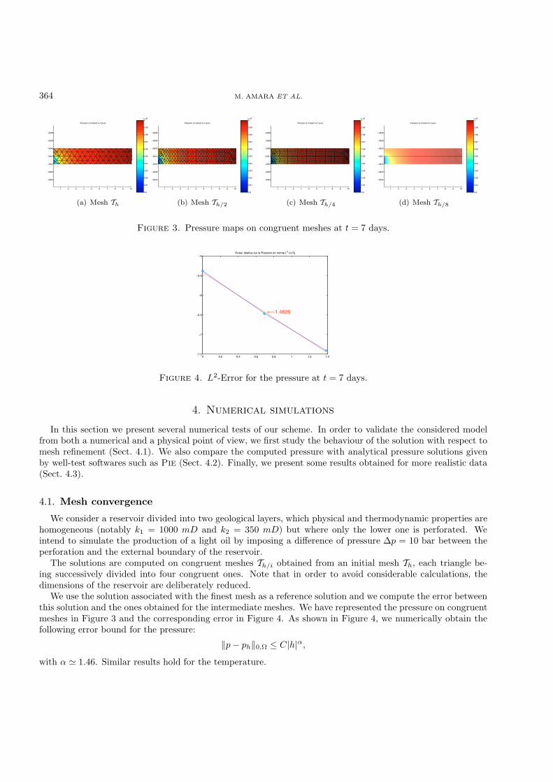
Figure 3. Pressure maps on congruent meshes at t = 7 days.

0 0.2 0.4 0.6 0.8 1 1.2 1.4−7.5

−7

−6.5

−6

−5.5

−5Erreur relative sur la Pression en norme L2 (t=7j)

←−1.4626

Figure 4. L2-Error for the pressure at t = 7 days.

4. Numerical simulations

In this section we present several numerical tests of our scheme. In order to validate the considered modelfrom both a numerical and a physical point of view, we first study the behaviour of the solution with respect tomesh refinement (Sect. 4.1). We also compare the computed pressure with analytical pressure solutions givenby well-test softwares such as Pie (Sect. 4.2). Finally, we present some results obtained for more realistic data(Sect. 4.3).

4.1. Mesh convergence

We consider a reservoir divided into two geological layers, which physical and thermodynamic properties arehomogeneous (notably k1 = 1000 mD and k2 = 350 mD) but where only the lower one is perforated. Weintend to simulate the production of a light oil by imposing a difference of pressure ∆p = 10 bar between theperforation and the external boundary of the reservoir.

The solutions are computed on congruent meshes Th/i obtained from an initial mesh Th, each triangle be-ing successively divided into four congruent ones. Note that in order to avoid considerable calculations, thedimensions of the reservoir are deliberately reduced.

We use the solution associated with the finest mesh as a reference solution and we compute the error betweenthis solution and the ones obtained for the intermediate meshes. We have represented the pressure on congruentmeshes in Figure 3 and the corresponding error in Figure 4. As shown in Figure 4, we numerically obtain thefollowing error bound for the pressure:

‖p − ph‖0,Ω ≤ C|h|α,

with α 1.46. Similar results hold for the temperature.

MIXED FINITE ELEMENT APPROXIMATION FOR A COUPLED PETROLEUM RESERVOIR MODEL 365

0 1 2 3 4 5 6 7 8 9 10−2845

−2844

−2843

−2842

−2841

−2840

−2839

−2838

−2837

Champ des vitesses au milieu des mailles à l’instant t=7 jours

(a) Velocity field

335.2

335.3

335.4

335.5

335.6

335.7

335.8

335.9

1 2 3 4 5 6 7 8 9 10

−2844

−2843

−2842

−2841

−2840

−2839

−2838

Température à l’instant t=7 jours

(b) Temperature map

Figure 5. Velocity and temperature on Th/2 at t = 7 days.

Figure 5 represents the velocity field and the temperature map after producing during one week.

4.2. Comparison with well-test softwares

Well-testing consists in varying the well flow rate, which disturbs the existing pressure in the reservoir,and then in measuring and interpreting the variations in pressure versus time to get information about thereservoir. To make well-test interpretation easier, different softwares such as Pie

1 are employed. For a givenflow rate history, they are notably able to analytically evaluate the distribution of pressure in the reservoir (cf.[3]) by using Fourier and Laplace transforms. Accordingly, these analytical simulators only work in simplifiedframeworks and do not take into account the energetic aspect.

Here, our aim is to compare our computed pressure with the one given by Pie.Thus, we treat the case of a mono-layer reservoir with constant physical and thermodynamic coefficients

and with horizontal and vertical permeabilities given by k1 = 100 mD and k2 = 1 mD. Moreover, the flow issupposed to verify the Darcy’s assumption and to be independent of the gravity effects, i.e. F = 0 and g = 0in (2).

First, we consider a reservoir characterized by a constant pressure (here pΓ = 360 bar) on its externalboundary. A production at constant flow rate (Q = 150 m3/day) is simulated during the first 24 hours and isfollowed by a shut-in period (Q = 0 m3/day) during the next 24 hours. As expected, we observe in Figure 6athat during the draw-down period, the flow regime goes through a transitory state to reach a permanent one.This permanent state is characterized by a constant wellbore pressure given by:

pwell = pΓ − αQBµ

Kh

(ln

R

rw+ S

), (16)

where α is a conversion factor, B is the volume factor, S is the skin (null in this experience) and rw, R respectivelyrefer to the wellbore and to the reservoir radius. Still in permanent regime, we can modify (16) to estimate, ata given z, the pressure at any r. Figure 6b shows that our solution (pink crosses) and the analytical one (ingreen) are very closed.

Next, we repeat the same experience for a closed reservoir. In other words, a no-flow condition G · n = 0 isnow set on the external boundary of the reservoir. As shown in Figure 7 and explained in Bourdarot [3], whilethe well is producing (the first 24 hours) the flow regime becomes pseudosteady-state as soon as the reservoirboundaries are reached. Moreover, while the well is shut-in (the last 24 hours), the pressure stabilizes at a valuecalled average pressure in the whole area defined by the no-flow boundaries.

1www.welltestsolutions.com

366 M. AMARA ET AL.

0 6 12 18 24 30 36 42 48315

320

325

330

335

340

345

350

355

360

365

Temps (en h)

Pre

ssio

n (e

n ba

r)

Comparaison avec PIE : Réservoir alimenté à pression constante

Solution PIESolution Axisymétrique

(a) Pressure evolution during 24h

0 10 20 30 40 50 60 70 80 90 100315

320

325

330

335

340

345

350

355

360Pression fonction du rayon en régime permanent

Rayon (en m)

pression puits : 319.8119

Pre

ssio

n (e

n ba

r)

Pression axisymétriquePression analytique

(b) Pressure at a given z, in a per-manent regime

Figure 6. Reservoir with a constant pressure boundary. Comparison of pressures.

0 6 12 18 24 30 36 42 48290

300

310

320

330

340

350

360

Temps (en h)

Pre

ssio

n (e

n ba

r)

Comparaison avec PIE : Réservoir fermé

Solution PIESolution Axisymétrique

Figure 7. Closed reservoir evolution in time of the pressure near the well.

4.3. Realistic reservoir

Let us now present a more realistic example. Our aim is to model an existing reservoir which is divided intoseven geological layers characterized by high heterogeneities concerning the physical properties (cf. Fig. 8).Thus, the producing layers (here, the even-numbered ones) have high permeabilities (from 1 to 7 Darcy) andcan be separated by quasi-walls (for instance, the third layer from the top) with low porosity and permeability.We simulate the production of a light oil by imposing a gradient of pressure between the perforations and theexternal boundary of the reservoir.

As one can observe in Figure 9, the temperature and the pressure obtained for different meshes after aone-month production are physically acceptable.

Mesh Nodes Edges TrianglesMesh T1 173 458 286Mesh T2 575 1609 1035Mesh T3 2020 5832 3813

Figure 10 represents the transitory period at the end of which the pressure is stabilized, while Figure 11 showsthe behaviour of the reservoir temperature during a one-month production.

MIXED FINITE ELEMENT APPROXIMATION FOR A COUPLED PETROLEUM RESERVOIR MODEL 367

k1 = 7000 mD k2 = 350 mD φ = 0.20 sw = 0.15

k1 = 7000 mD k2 = 350 mD φ = 0.28 sw = 0.15

k1 = 10 mD k2 = 1 mD φ = 0.08 sw = 0.9

k1 = 1000 mD k2 = 15 mD φ = 0.24 sw = 0.42

k1 = 1000 mD k2 = 15 mD φ = 0.26 sw = 0.30

k1 = 1000 mD k2 = 15 mD φ = 0.22 sw = 0.38

k1 = 1000 mD k2 = 15 mD φ = 0.24 sw = 0.40

Figure 8. Vertical section of the reservoir.

5 10 15 20 25 30 35 40 45 50

−2850

−2845

−2840

−2835

−2830

−2825

−2820

−2815

Pression à l’instant t=28 jours

3.9

3.91

3.92

3.93

3.94

3.95

3.96

3.97

3.98

3.99

4x 10

7

(a) Pressure - Mesh T1

5 10 15 20 25 30 35 40 45 50

−2850

−2845

−2840

−2835

−2830

−2825

−2820

−2815

Pression à l’instant t=28 jours

3.9

3.91

3.92

3.93

3.94

3.95

3.96

3.97

3.98

3.99

4x 10

7

(b) Pressure - Mesh T2

5 10 15 20 25 30 35 40 45 50

−2850

−2845

−2840

−2835

−2830

−2825

−2820

−2815

Pression à l’instant t=28 jours

3.9

3.91

3.92

3.93

3.94

3.95

3.96

3.97

3.98

3.99

4x 10

7

(c) Pressure - Mesh T3

5 10 15 20 25 30 35 40 45 50

−2850

−2845

−2840

−2835

−2830

−2825

−2820

−2815

Température à l’instant t=28 jours

333.5

334

334.5

335

335.5

336

336.5

(d) Temperature - Mesh T1

5 10 15 20 25 30 35 40 45 50

−2850

−2845

−2840

−2835

−2830

−2825

−2820

−2815

Température à l’instant t=28 jours

333.5

334

334.5

335

335.5

336

336.5

(e) Temperature - Mesh T2

5 10 15 20 25 30 35 40 45 50

−2850

−2845

−2840

−2835

−2830

−2825

−2820

−2815

Température à l’instant t=28 jours

333.5

334

334.5

335

335.5

336

336.5

(f) Temperature - Mesh T3

Figure 9. Pressure and temperature maps at t = 28 days, for realistic data.

4.4. Influence of the permeability

As one can notice from the previous examples, when treating a reservoir associated with a vertical wellbore,one generally has that k1 k2 where k1 is the radial permeability and k2 the vertical one. However, inorder to numerically validate the code, we next present an example where k2 k1. More precisely, we takek1 = 1 mD whereas k2 = 1000 mD. Since the flow is mainly radial, the influence of the radial permeability k1

is preponderant compared with the one of the vertical permeability k2, which leads to similar results from aqualitative point of view for both situations k2 k1 and k2 k1 (cf. Fig. 12).

368 M. AMARA ET AL.

5 10 15 20 25 30 35 40 45 50

−2850

−2845

−2840

−2835

−2830

−2825

−2820

−2815

Pression à l’instant t=0.1 minute

3.9

3.91

3.92

3.93

3.94

3.95

3.96

3.97

3.98

3.99

4x 10

7

(a)

5 10 15 20 25 30 35 40 45 50

−2850

−2845

−2840

−2835

−2830

−2825

−2820

−2815

Pression à l’instant t=0.5 minutes

3.9

3.91

3.92

3.93

3.94

3.95

3.96

3.97

3.98

3.99

4x 10

7

(b)

5 10 15 20 25 30 35 40 45 50

−2850

−2845

−2840

−2835

−2830

−2825

−2820

−2815

Pression à l’instant t=3 minutes

3.9

3.91

3.92

3.93

3.94

3.95

3.96

3.97

3.98

3.99

4x 10

7

(c)

Figure 10. The pressure reaching steady state.

5 10 15 20 25 30 35 40 45 50

−2850

−2845

−2840

−2835

−2830

−2825

−2820

−2815

Température à l’instant t=0 jour

335.2

335.4

335.6

335.8

336

336.2

(a) t=0 day

5 10 15 20 25 30 35 40 45 50

−2850

−2845

−2840

−2835

−2830

−2825

−2820

−2815

Température à l’instant t=7 jours

335.2

335.4

335.6

335.8

336

336.2

(b) t=7 days

5 10 15 20 25 30 35 40 45 50

−2850

−2845

−2840

−2835

−2830

−2825

−2820

−2815

Température à l’instant t=28 jours

335.2

335.4

335.6

335.8

336

336.2

(c) t=28 days

Figure 11. Behaviour of the reservoir temperature during a one-month production.

5 10 15 20 25 30 35 40 45 50

−2820

−2815

−2810

−2805

−2800

−2795

−2790

Pression à l’instant t=7 jours

3.91

3.92

3.93

3.94

3.95

3.96

3.97

3.98

3.99

4

x 107

(a) Pressure

5 10 15 20 25 30 35 40 45 50

−2820

−2815

−2810

−2805

−2800

−2795

−2790

Température à l’instant t=7 jours

335.2

335.3

335.4

335.5

335.6

335.7

(b) Temperature

Figure 12. A one-layer reservoir with k2 k1.

Finally, we detail an example where the permeability is extremely different in the layers. This aspect wasalready encountered to a lesser extent when studying the realistic case.

We take for that a two-layer reservoir with (k1, k2) = (5000 mD, 350 mD) for the first layer and (1 mD, 1 mD)for the second one, and we impose a difference of pressure between the perforation and the external boundaryof the reservoir. The layers are both perforated but due to a better permeability, the flow mainly takes placethrough the first layer, which leads to a higher rise in the temperature as shown in Figure 13.

MIXED FINITE ELEMENT APPROXIMATION FOR A COUPLED PETROLEUM RESERVOIR MODEL 369

5 10 15 20 25 30 35 40 45 50

−2820

−2815

−2810

−2805

−2800

−2795

−2790

Pression à l’instant t=7 jours

3.91

3.92

3.93

3.94

3.95

3.96

3.97

3.98

3.99

4

x 107

(a) Pressure

5 10 15 20 25 30 35 40 45 50

−2820

−2815

−2810

−2805

−2800

−2795

−2790

Température à l’instant t=7 jours

335.2

335.3

335.4

335.5

335.6

335.7

335.8

(b) Temperature

Figure 13. Two-layer reservoir with heterogeneous permeability.

5. A POSTERIORI error estimators

We define in this section reliable and efficient a posteriori estimators, which can be used for local meshrefinements and implicitly for improvement of the solution.

It is useful to write the discrete problem (14) under the equivalent form:

Find σh ∈ V

∗h × Lh

Ah(σh, σ′h) = Fh(σ′

h), ∀σ′h ∈ V

0h × Lh,

(17)

where σh = (Vh, sh), Ah =[

A B−BT (C + Dh)

]and Fh =

(F1h

F2h + F3h

).

5.1. Mesh-dependent norms and error indicators

In order to define a posteriori error indicators on the Raviart-Thomas finite element space Vh, we applysome results of Verfurth and Braess [13]. We begin by introducing the following mesh-dependent norms:

|||V|||h =

(‖G‖2

0,Ω + ‖q‖20,Ω +

∑e∈Eh

he‖G · n‖20,e +

∑e∈Eh

he‖q · n‖20,e

)1/2

, ∀V = (G,q) ∈ V0h,

|s|1,h =

( ∑K∈Th

|p|21,K +∑

K∈Th

|T |21,K +∑e∈Eh

h−1e ‖[p]‖2

0,e +∑e∈Eh

h−1e ‖[T ]‖2

0,e

)1/2

, ∀s = (p, T ) ∈ Lh,

(18)

where [p] represents the jump of p across an internal edge e, respectively the trace of p if e ⊂ ∂Ω.Then the following equivalences of norms hold:

‖V‖0,Ω ≤ |||V|||h ≤ c‖V‖0,Ω, ∀V ∈ V0h, (19)

‖s‖0,Ω ≤ ch|s|1,h ≤ c′‖s‖0,Ω, ∀s ∈ Lh, (20)

with c, c′ independent of h. We refer for instance to Roberts and Thomas [12] for the proof of (19) and (20).

370 M. AMARA ET AL.

Moreover, one has:

|B(s,V)| ≤ c|||V|||h|s|1,h, ∀V ∈ V0h, ∀s ∈ Lh, (21)

supV∈V0

h

B(s,V)|||V|||h

≥ c|s|1,h, ∀s ∈ Lh, (22)

where the first statement is obvious and the second one is established, for instance, in Verfurth and Braess [13].Finally, the above inequalities ensure that the bilinear forms A(·, ·) and B(·, ·) satisfy the Babuska-Brezzi

conditions with respect to the discrete norms ||| · |||h and | · |1,h.Concerning the continuity of (C + Dh)(·, ·) with respect to the norm | · |1,h, one can easily show that:

C(s, s′) + Dh(s, s′) ≤(

c1h2

∆t+ c2‖Gn−1

h ‖0,Ω

)|s|1,h|s′|1,h, ∀s, s′ ∈ Lh,

therefore its continuity constant depends on h2

∆t . However, the norm of the inverse operator A−1h being inde-

pendent of the norm of C + Dh, the following stability property is true:

|||V|||h + |s|1,h ≤ c sup(V′,s′)∈V0

h×Lh

Ah((V, s), (V′, s′))|||V′|||h + |s′|1,h

, ∀(V, s) ∈ V0h × Lh (23)

with a constant c which only depends on the thermodynamic coefficients.Let us proceed with the a posteriori error analysis. For that, we introduce the following residuals on any

triangle K ∈ Th and any edge e ∈ Eh:

ηK,1 =

(∥∥∥∥1rMGh + ∇ph − ρn−1h g

∥∥∥∥2

0,K

+∥∥∥∥ 1

rλqh −∇Th

∥∥∥∥2

0,K

)1/2

,

ηK,2 =

(∥∥∥∥r a

∆tph − r

b

∆tTh + divGh − r

a

∆tpn−1

h + rb

∆tT n−1

h

∥∥∥∥2

0,K

+

∥∥∥∥∥rd

∆tTh − r

f

∆tph +

k

|K|∑

e∈∂K−

∫e

(Gn−1

h · n)ηe,2dσ

+l

|K|∑

e∈∂K−

∫e

(Gn−1

h · n)ηe,1dσ − divqh − r

d

∆tT n−1

h + rf

∆tpn−1

h

∥∥∥∥2

0,K

)1/2

,

ηe =(‖ηe,1‖2

0,e + ‖ηe,2‖20,e

)1/2,

where

ηe,1 =

ph − pΓ if e ⊂ Γp

0 if e ⊂ ∂Ω\Γp

[ph] if e ∈ E0h

, ηe,2 =

Th − TΓ if e ⊂ ΓT

0 if e ⊂ ∂Ω\ΓT

[Th] if e ∈ E0h

.

MIXED FINITE ELEMENT APPROXIMATION FOR A COUPLED PETROLEUM RESERVOIR MODEL 371

The local error indicator is a weighted combination:

ηK =

(η2

K,1 + h2Kη2

K,2 +∑

e∈∂K

h−1e η2

e

)1/2

,

and the global one is given by:

η =

[ ∑K∈τh

(η2

K,1 + h2Kη2

K,2

)+∑e∈Eh

h−1e η2

e

]1/2

.

According to [13], we make the following saturation assumption (SA): ∃β < 1 such that

|||V − Vh/2|||h/2 + |s − sh/2|1,h/2 ≤ β(|||V − Vh|||h/2 + |s − sh|1,h/2

),

where Th/2 is obtained from Th by dividing each triangle into four congruent ones and where σh/2 = (Vh/2, sh/2)is the unique solution of the variational problem:

Find σh/2 ∈ V∗h/2 × Lh/2

Ah/2(σh/2, σ′) = Fh/2(σ′), ∀σ′ ∈ V

0h/2 × Lh/2,

(24)

with Ah/2 =[

A B−BT C + Dh/2

]and Fh/2 =

(F1h

F2h + F3h/2

).

We took the same right-hand side terms F1h, F2h as in (17), since they only depend on discrete quantitiesalready computed at tn−1, but we redefined on Th/2 the terms arising from the upwind scheme.

5.2. Error analysis

We first establish an upper bound for the error. One immediately gets (see for instance [13]):

|||G′|||h/2 ≤ |||G′|||h ≤√

2|||G′|||h/2, ∀G′ ∈ Vh, (25)1√2|p′|1,h/2 ≤ |p′|1,h ≤ |p′|1,h/2, ∀p′ ∈ Lh. (26)

Then the following statement holds:

Theorem 5.1. One has that:

|||Vh/2 −Vh|||h + |sh/2 − sh|1,h/2 ≤ cη,

with c independent of the discretization and of ∆t.

Proof. Using the stability property (23) for the problem (24) and the fact that Vh −Vh/2 ∈ V0h, one has that:

|||Vh − Vh/2|||h/2 + |sh − sh/2|1,h/2 ≤ c sup(V′,s′)∈V

0h/2×Lh/2

Ah/2((Vh − Vh/2, sh − sh/2), (V′, s′))

|||V′|||h/2 + |s′|1,h/2

·

372 M. AMARA ET AL.

Let us estimate:

Ah/2((Vh − Vh/2, sh − sh/2), (V′, s′)) = A(Vh,V′) + B(sh,V′) − B(s′,Vh)

+ (C + Dh/2)(sh, s′h/2) − F1h(V′) − F2h(s′) − F3h/2(s′).

For that, we integrate by parts:

B(sh,V′) =∑

e∈E0h∪Γp

∫e

G′ · n[ph]dσ −∑

e∈E0h∪ΓT

∫e

q′ · n[Th]dσ

and we take into account the boundary terms of F1h(·). The Cauchy-Schwarz inequality then gives that:

A(Vh,V′) + B(sh,V′) − F1h(V′)

≤∑

K∈Th

η1,K‖V′‖0,K +

(∑e∈Eh

he‖G′ · n‖20,e + he‖q′ · n‖2

0,e

)1/2(∑e∈Eh

h−1e η2

e

)1/2

≤( ∑

K∈Th

η21,K +

∑e∈Eh

h−1e η2

e

)1/2(‖V′‖2

0,Ω +∑e∈Eh

he‖G′ · n‖20,Ω + he‖q′ · n‖2

0,Ω

)1/2

≤ η|||V′|||h.

In the same manner, one may write that:

−B(s′,Vh) + (C + Dh/2)(sh, s′) − F2h(s′) − F3h/2(s′)

= −B(s′,Vh) + (C + Dh)(sh, s′) − F2h(s′) − F3h(s′) + (Dh/2 − Dh)(sh, s′) + (F3h − F3h/2)(s′)

≤∑

K∈Th

η2,K‖s′‖0,Ω + (Dh/2 − Dh)(sh, s′) + (F3h − F3h/2)(s′)

≤( ∑

K∈Th

h2Kη2

2,K

)1/2

|s′|1,h + (Dh/2 − Dh)(sh, s′) + (F3h − F3h/2)(s′).

By using the continuity of Dh(·, ·) and F3h(·) (see the proof of Lem. 3.2) and the relations (25) and (26), onehas that:

Dh(sh, s′) − F3h(s′) ≤ c‖Gn−1h ‖0,Ω|s′|1,h/2

(∑e∈Eh

h−1e η2

e

)1/2

,

and similarly,

Dh/2(sh, s′) − F3h/2(s′) ≤ c′‖Gn−1h ‖0,Ω|s′|1,h/2

(∑e∈Eh

h−1e η2

e

)1/2

.

Therefore, it now comes that:

−B(s′, Vh) + (C + Dh/2)(sh, s′) − F2h(s′) − F3h/2(s′) ≤ c

( ∑K∈Th

h2Kη2

2,K +∑e∈Eh

h−1e η2

e

)1/2

|s′|1,h/2 ,

MIXED FINITE ELEMENT APPROXIMATION FOR A COUPLED PETROLEUM RESERVOIR MODEL 373

and finally:

Ah/2((Vh − Vh/2, sh − sh/2), (V′, s′)) ≤ cη(|s′|1,h/2 + |||V′|||h/2),

with c depending on ‖Gn−1h ‖0,Ω. This last estimate leads to the conclusion.

By applying the triangle inequality and the saturation assumption (SA), one can now deduce an upperestimate for the error in weighted norms:

Theorem 5.2. The following error bound holds:

|||V −Vh|||h + |s − sh|1,h ≤ c

1 − βη.

Concerning a lower bound for the error, this is easily obtained thanks to the definition of the discrete weightednorms. Indeed, the regularity of the continuous time-discretized problem (7) gives s ∈ H

1(Ω), therefore by thetrace theorem one gets that [sh] = [sh − s] on every internal edge e ∈ E0

h. So,

(∑e∈Eh

h−1e η2

e

)1/2

≤ |sh − s|1,h. (27)

Moreover, since the exact solution (V, s) satisfies:

1rMG + ∇p − ρn−1g = 0 and

1rλ

q −∇T = 0 a.e. in Ω,

one may write that:

η2K,1 =

∥∥∥∥∇(p − ph) +1rM(G − Gh) − (ρn−1 − ρn−1

h )g∥∥∥∥

2

0,K

+∥∥∥∥∇(T − Th) +

1rλ

(q − qh)∥∥∥∥

2

0,K

≤ c(|p − ph|21,K + |T − Th|21,K + ‖G− Gh‖2

0,K + ‖q− qh‖20,K + ‖ρn−1 − ρn−1

h ‖20,K

).

Hence, ( ∑K∈Th

η2K,1

)1/2

≤ c(|s − sh|1,h + |||V− Vh|||h + ‖ρn−1 − ρn−1

h ‖0,Ω

). (28)

In order to bound the last residual ηK,2, we use that divGh ∈ Lh, for all Gh ∈ Vh. Then the last variationalequation of (14) gives, on every K ∈ Th:

divGh = Ph

(ra

∆tpn−1

h − rb

∆tT n−1

h

)− Ph

(ra

∆tph − rb

∆tTh

),

divqh = Ph

(rd

∆tTh − rf

∆tph

)− Ph

(rd

∆tT n−1

h − rf

∆tpn−1

h

)

+k

|K|∑

e∈∂K−

∫e

(Gn−1

h · n)ηe,2dσ +

l

|K|∑

e∈∂K−

∫e

(Gn−1

h · n)ηe,1dσ,

with Ph : L2(Ω) −→ Lh the piecewise constant L2-orthogonal projection operator.

374 M. AMARA ET AL.

Then by replacing divqh and divGh in ηK,2, it comes that:

η2K,2 ≤

∥∥∥∥(

a

∆tpn−1

h − b

∆tT n−1

h − a

∆tph +

b

∆tTh

)(r − Phr)

∥∥∥∥2

0,K

+∥∥∥∥(

d

∆tTh − f

∆tph − d

∆tT n−1

h +f

∆tpn−1

h

)(r − Phr)

∥∥∥∥2

0,K

≤ c

∆t2‖r − Phr‖2

0,K

and finally,

( ∑K∈Th

h2η2K,2

)1/2

≤ ch2

∆t· (29)

By putting together (27), (28) and (29), we have thus established:

Theorem 5.3. The error estimator η yields the following global, respectively local, lower bounds:

η ≤ c(|||V− Vh|||h + |s − sh|1,h + ‖ρn−1

h − ρn−1‖0,Ω

)+

ch2

∆t

ηK ≤ c(|||V −Vh|||h,ωK + |s − sh|1,h,ωK + ‖ρn−1

h − ρn−1‖0,K

)+

ch2

∆t

where ωK is the set of the triangles K ′ ∈ Th, neighbours of K and c is independent of h and ∆t.

Remark 5.4. One can also consider a posteriori error estimates with respect to the natural norms of H(div, Ω)and L

2(Ω) (see [2]). Then following Verfurth and Braess [13], one can obtain under a saturation assumptionthat:

|||V− Vh||| + ‖s − sh‖0,Ω ≤ cη +c

h‖Gn−1

h ‖0,e

(∑e∈Eh

h−1e η2

e

)1/2

,

where η is defined by:

η =

( ∑K∈Th

η2K,1 +

∑K∈Th

η2K,2 +

∑e∈Eh

h−1e η2

e

)1/2

.

A lower bound can also be obtained but is not optimal.

5.3. Numerical results

We consider the same case of oil production as the one presented in Section 4.3.In Figure 14, we represent the local estimators ηK , ηK,1, ηK,2 and (

∑e∈∂K h−1

e η2e)1/2 calculated for different

meshes T1, T2 and T3 introduced in Section 4.3, after a one-month production. The approximate pressure andtemperature on the previous meshes were given in Figure 9.

MIXED FINITE ELEMENT APPROXIMATION FOR A COUPLED PETROLEUM RESERVOIR MODEL 375

5 10 15 20 25 30 35 40 45 50

−2850

−2845

−2840

−2835

−2830

−2825

−2820

−2815

ηK à l’instant t=28 jours

6

7

8

9

10

11

12

13

14

15

16

(a) ηK - Mesh T1

5 10 15 20 25 30 35 40 45 50

−2850

−2845

−2840

−2835

−2830

−2825

−2820

−2815

ηK à l’instant t=28 jours

6

7

8

9

10

11

12

13

14

15

16

(b) ηK - Mesh T2

5 10 15 20 25 30 35 40 45 50

−2850

−2845

−2840

−2835

−2830

−2825

−2820

−2815

ηK à l’instant t=28 jours

6

7

8

9

10

11

12

13

14

15

16

(c) ηK - Mesh T3

5 10 15 20 25 30 35 40 45 50

−2850

−2845

−2840

−2835

−2830

−2825

−2820

−2815

ηK1

à l’instant t=28 jours

6

8

10

12

14

16

(d) ηK,1 - Mesh T1

5 10 15 20 25 30 35 40 45 50

−2850

−2845

−2840

−2835

−2830

−2825

−2820

−2815

ηK1

à l’instant t=28 jours

6

8

10

12

14

16

(e) ηK,1 - Mesh T2

5 10 15 20 25 30 35 40 45 50

−2850

−2845

−2840

−2835

−2830

−2825

−2820

−2815

ηK1

à l’instant t=28 jours

6

8

10

12

14

16

(f) ηK,1 - Mesh T3

5 10 15 20 25 30 35 40 45 50

−2850

−2845

−2840

−2835

−2830

−2825

−2820

−2815

ηK2

à l’instant t=28 jours

−8

−6

−4

−2

0

2

(g) ηK,2 - Mesh T1

5 10 15 20 25 30 35 40 45 50

−2850

−2845

−2840

−2835

−2830

−2825

−2820

−2815

ηK2

à l’instant t=28 jours

−8

−6

−4

−2

0

2

(h) ηK,2 - Mesh T2

5 10 15 20 25 30 35 40 45 50

−2850

−2845

−2840

−2835

−2830

−2825

−2820

−2815

ηK2

à l’instant t=28 jours

−8

−6

−4

−2

0

2

(i) ηK,2 - Mesh T3

5 10 15 20 25 30 35 40 45 50

−2850

−2845

−2840

−2835

−2830

−2825

−2820

−2815

sum(1/he * η

e2) à l’instant t=28 jours

12

14

16

18

20

22

24

26

28

30

(j) (∑

e∈∂K h−1e η2

e )1/2 - Mesh T1

5 10 15 20 25 30 35 40 45 50

−2850

−2845

−2840

−2835

−2830

−2825

−2820

−2815

sum(1/he * η

e2) à l’instant t=28 jours

12

14

16

18

20

22

24

26

28

30

(k) (∑

e∈∂K h−1e η2

e)1/2 - Mesh T2

5 10 15 20 25 30 35 40 45 50

−2850

−2845

−2840

−2835

−2830

−2825

−2820

−2815

sum(1/he * η

e2) à l’instant t=28 jours

12

14

16

18

20

22

24

26

28

30

(l) (∑

e∈∂K h−1e η2

e)1/2 - Mesh T3

Figure 14. Local estimators for different mesh refinements.

As expected, the quality of the estimators increases with the mesh refinement. Moreover, one can notice thatthe area requiring a local refinement of the mesh is the one located near the wellbore, i.e. where the velocity isthe highest.

376 M. AMARA ET AL.

References

[1] C. Abchir, Modelisation des ecoulements dans les reservoirs souterrains avec prise en compte des interactions puits/reservoir.These de doctorat, Universite de Saint-Etienne (1992).

[2] M. Amara, D. Capatina, B. Denel and P. Terpolilli, Modelling, analysis and numerical approximation of flow with heat transferin a petroleum reservoir, Preprint No. 0415, Universite de Pau (2004) (http://lma.univ-pau.fr/publis/publis.php).

[3] G. Bourdarot, Well testing: Interpretation methods. Editions Technip, Paris (1998).[4] S. Brenner and R. Scott, The mathematical theory of Finite Element Methods. Springer Verlag, New York (1994).[5] F. Brezzi and M. Fortin, Mixed and Hybrid Finite Element Methods. Springer Verlag, New York (1991).[6] G. Chavent and J.E. Roberts, A unified physical presentation of mixed, mixed-hybrid finite elements and standard finite

difference approximations for the determination of velocities in waterflow problems. Adv. Water Resources 14 (1991) 329–348.[7] P.G. Ciarlet, The finite element method for elliptic problems error analysis. North Holland, Amsterdam (1978).[8] R.E. Ewing, J. Wang and S.L. Weekes, On the simulation of multicomponent gas flow in porous media. Appl. Numer. Math.

31 (1999) 405–427.[9] P. Grisvard, Elliptic problems on non-smooth domains. Pitman, Boston (1985).

[10] F. Maubeuge, M. Didek, E. Arquis, O. Bertrand and J.-P. Caltagirone, Mother: A model for interpreting thermometrics. SPE28588 (1994).

[11] D.Y. Peng and D.B. Robinson, A new two-constant equation of state. Ind. Eng. Chem. Fundam. 15 (1976) 59–64.[12] J.E. Roberts and J.-M. Thomas, Mixed and Hybrid Methods, in Handbook of Numerical Analysis Vol. II. North Holland,

Amsterdam (1991) 523–639.[13] R. Verfurth and D. Braess, A posteriori error estimator for the Raviart-Thomas element. SIAM J. Numer. Anal. 33 (1996)

2431–2444.

To access this journal online:www.edpsciences.org