Interactive Implicit Modeling With Hierarchical Spatial C aching

Ryan SchmidtUniversity of Calgary

Computer Sciencerms@cpsc.ucalgary.ca

Brian WyvillUniversity of Calgary

Computer Scienceblob@cpsc.ucalgary.ca

Eric GalinLIRIS - CNRS

Universite Claude Bernard Lyon 1eric.galin@liris.cnrs.fr

Abstract

Interactive modeling using implicit surfaces requires afast visualization technique. Complex implicit CSG modelscan be represented hierarchically as a tree of nodes (theBlobTree) . However, current methods cannot be used to vi-sualize changes made to these models at interactive ratesdue to the large number of potential field evaluations re-quired. We present a heirarchical spatial caching techniquewhich accelerates evaluations of the potential function. Themethod introduces the concept of a caching node insertedinto the implicit model tree. Caching nodes store exact po-tential field values at the nodes of a voxel grid and rely ontri-linear and tri-quadratic reconstruction filters to locallyapproximate the potential field of a sub-tree. The cachingnodes employ a lazy evaluation scheme to avoid expensivepre-computation.

With spatial caching nodes an order-of-magnitude de-crease in polgyonization time is achieved for complex im-plicit models containing thousands of primitives. Interactivemanipulation of these models is demonstrated in a BlobTreemodeling tool.

1. Introduction

Interactive modeling is an iterative, essentially trial-and-error process. Components of complex models are createdindependently and then assembled. A significant portion ofthe designer’s time is spent making small changes to modelparameters and examining the results. To facilitate this kindof interaction, interactive visual feedback is necessary.

Implicit surface modeling has been hampered by thelack of a fast interactive visualization method. Local-updatemethods [9] are effective only when the underlying modeltree is simple. Particularly when assembling the compo-nents of a complex model, computing a single field valuefor a complex model can require an immense number ofleaf-node field evaluations and composition operations.

Standard implicit surface visualization methods rely oncomputing the value and gradient of the scalar field manytimes. In profiling implicit surface polygonizers, we observethat over 95% of the computation time is spent in field valueevaluations. Potential field function evaluation time mustbereduced in order to provide interactive visual feedback thatscales to complex models.

In this paper we propose a hierarchical spatial cachingtechnique that can be used to greatly decrease the numberof tree nodes traversed when computing a single field valueor gradient. We implement spatial caches using uniform 3Dgrids, storing field values at grid vertices. Tri-linear andtri-quadratic reconstruction filters are applied to these cachedfield values to locally approximate the potential field thatdefines the implicit surface. Using this process the compu-tational complexity of a single field evaluation for a cachedsub-tree is reduced fromO(n) to O(1), wheren refers tothe number of nodes in the subtree. Our results show thatthis caching technique is capable of providing an order-of-magnitude decrease in interactive polygonization time forcomplex hierarchical skeletal implicit models.

The remainder of this paper will proceed as follows. Insection 2 we will describe related work. Section 3 describesthe fundamentals of the BlobTree modeling system. Sec-tion 4 introduces spatial caching nodes to the BlobTree andaddresses the spatial caching process. Section 5 describessome implementation details regarding memory considera-tions. Results and future work are covered in sections 6 and7, respectively.

2. Related Work

A variety of implicit surface modeling systems havebeen proposed in the last decade. These systems use var-ious underlying implicit representations. A small sampleincludes skeletal elements [19], levels sets [14], con-volution surfaces [4] [11], adaptive distance fields [10]variational implicit surfaces [16], and functional represen-tations [15].

All of these systems can be used to model com-

plex shapes. Recent interactive sculpting [7] [3] andsketch-based modeling [12] [1] systems provide interactivevisualization rates while updating the implicit model. How-ever, fundamentally these systems construct global models.By this we mean that the final implicit model is not com-posed of smaller components that can be individuallymanipulated, but rather a single volume. A more gen-eral implicit modeling system such as the BlobTree [19] isrequired to combine these elements into a complex hierar-chical model.

Unfortunately, no scalable interactive visualization tech-nique for complex BlobTree models exist. The key issue isthat the functionally-defined implicit surface must be con-verted to a discrete representation, such as a triangle meshor point set, to be visualized on commodity graphics hard-ware. This surface extraction process is too computation-ally demanding to execute in real time as a designer inter-actively modifies a complex implicit model.

One avenue for reducing surface extraction time is to in-crementally compute a new surface discretization as localchanges are made by the designer. Some proposed tech-niques include incremental octree subdivision of space [8],adaptive marching triangles approaches [9], and sur-face constrained particle systems [18]. Interactive perfor-mance has been demonstrated for relatively simple mod-els. However, incremental update schemes do not scale tocomplex hierarchical models because the cost of evaluat-ing even the local update region becomes too expensive.In addition, large-scale model changes are not acceler-ated.

Level-of-detail schemes for implicit surfaces [?] [11] at-tempt to speed up potential field queries by dynamicallyreducing the complexity of the implicit model tree. Thesetechniques reducing interactive visualization times whenlower levels of detail can be used. Our technique can be usedin conjunction with these methods to reduce polygonizationtime at all levels of detail.

Our goal is to enable interactive modeling of compleximplicit surfaces by accelerating potential field queries.Weuse potential field function approximations similar to [3],where the implicit model was stored as a set of potentialfield value samples in a uniform 3D grid. A smoothC1 con-tinuous surface was extracted from these samples using re-construction filters. We adapt this technique to dynamicallyconstruct spatial caches in our heirarchical model. We ap-proximate the potential field function whenever possible,avoiding the complex tree traversals required when evalu-ate a potential field query. This work is in spirit related tothe render cache system [17] that exist for speeding up in-teractive ray-racing applications.

3. The BlobTree

An implicit surface is mathematically defined as thepoints in space that satisfy the equation

S = {p ∈ R3, f(p) − T = 0}

wheref(p) denotes a scalar field function in space andT athreshold value. The BlobTree model [19] is characterizedby a hierarchical combination of primitives organized in atree data-structure (Figure 1). The nodes of the tree includeblending, Boolean and warping nodes, whereas the leavesare skeletal elements.

Blend

Union

Difference

Figure 1. A simplified representation of the treestructure of a bottle

Skeletal elements are defined by a skeleton, a distancefunction and a potential field function with a compact sup-port. Therefore, every skeletal primitive has a boundedregion of influence in space. Every node incorporates abounding box so as to rapidly discard useless field func-tion evaluations when queries are performed in empty re-gions of space.

The computation of the field functionf(p) at a givenpoint in space is performed by recursively traversing theBlobTree structure. The skeletal primitives at the leaves ofthe tree return potential field values, which are combined bythe operators at the nodes of the tree.

Field function evaluation is the most computationally de-manding step in every application. Ray tracing techniquesrequire many field function evaluations along a ray to iso-late the roots and converge to the ray-implicit surface in-tersection. Polygonization techniques also query the Blob-Tree with many potential field function evaluations. There-fore, it is crucial to be able to accelerate the computation off(p) for interactive modeling applications.

4. Hierarchical spatial caching

Hierarchical spatial caching is integrated into the Blob-Tree implicit modeling framework by introducing cachingnodes. A caching nodeC is a unary operator with a sin-gle subtreeT . Each caching node stores a set of exact po-tential field values determined by querying it’s subtreeT .When evaluating the potential field ofT at a pointp in-side the bounding box ofT , an approximationfC(p) to theexact potential field valuefT (p) is reconstructed from thecached potential values. The subtreeT is not traversed.

In the next sections we will describe in detail our imple-mentation of caching nodes.

4.1. Data structure

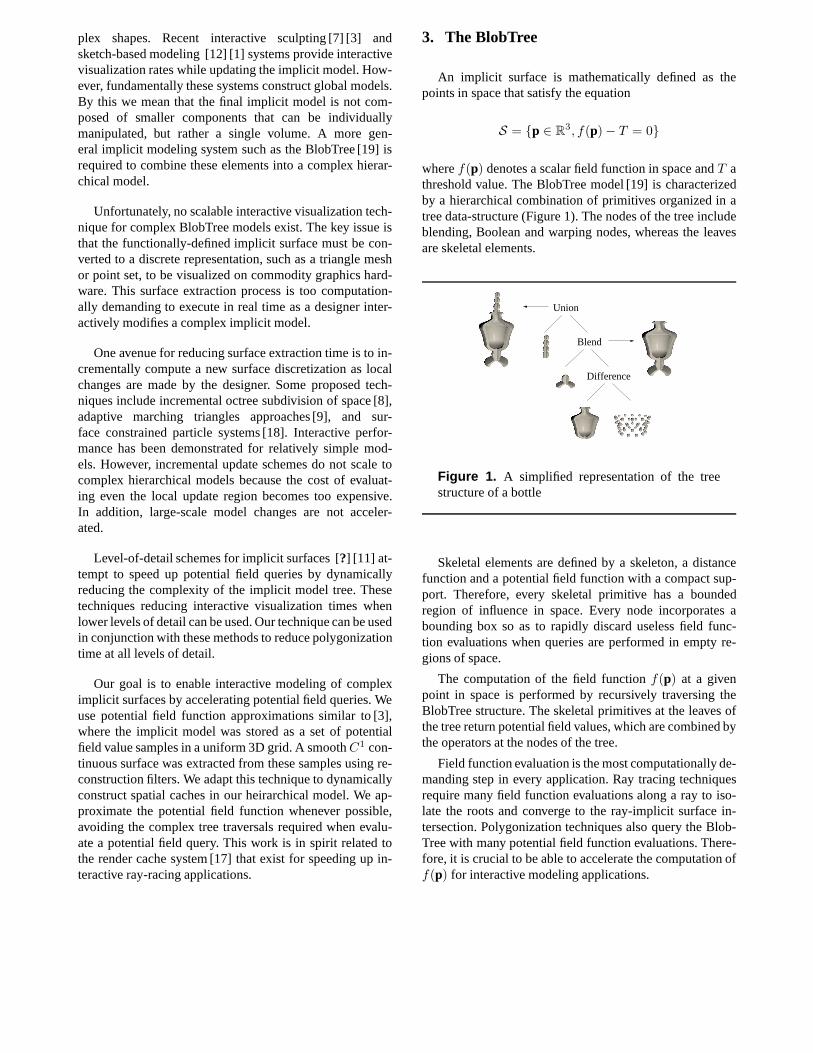
In our system caching nodes are inserted above compo-sition nodes. We specifically do not place a caching nodeat the root of the tree, as this cache would require continu-ous updating in an interactive system. Our caching nodesstore the exact potential field values at the nodes of avoxel grid (Figure 2). In the remainder of this sectionpijk,(i, j, k) ∈ [0, n]3 will refer to a point in the voxel grid. Thecorresponding potential field value stored atpijk will be de-noted asvijk = fT (pijk).

Difference

Blend

Union

Cache

Cache

Figure 2. A bottle model with some cache nodes.The cache resolution for a subtreeT is dependent onthe subtree size

Each caching node has a local reference frame, allowingthe uniform grid to be rotated and translated in line with theorientation of it’s subtreeT . This avoids expensive cacherecalculation when the entire sub-tree is manipulated.

When some descendent node of a caching node changes,the bounding box of the descendent node is used to locallyinvalidate cached values in all parent caches. Invalidation

is carried out at each cache by clearing avalid flag for allcached values inside the bounding box.

4.2. Caching algorithm

Caching nodes are implemented using reconstruction fil-ters R that approximate the field functionfT (p) usingnearby exact field value samples(pijk, vijk) of the subtreeT . Approximating the field function of the subtreefT (p)by fC(p) is more efficient only if the necessary field valuesamples(pijk , vijk) have been pre-computed.

The steps taken by a cache node to computefC(p) are asfollows:

1. Transformp into local cache coordinatesp′

2. If the necessary field value samples(pijk , vijk) re-quired to evaluateR(p′) are cached, go to step 4

3. Cache any missing field value samples(pijk, vijk) byevaluating the subtree.

4. Evaluate the reconstruction filterR(p′)

4.3. Lazy evaluation

The initial field values used by spatial cache nodes to cal-culate interpolated field values are found by evaluating thechild node’s field value. For complex sub-trees these eval-uations can be quite expensive. The overhead necessary tocreate and maintain a fully-evaluated uniform grid spatialcache has a significant impact on interactivity.

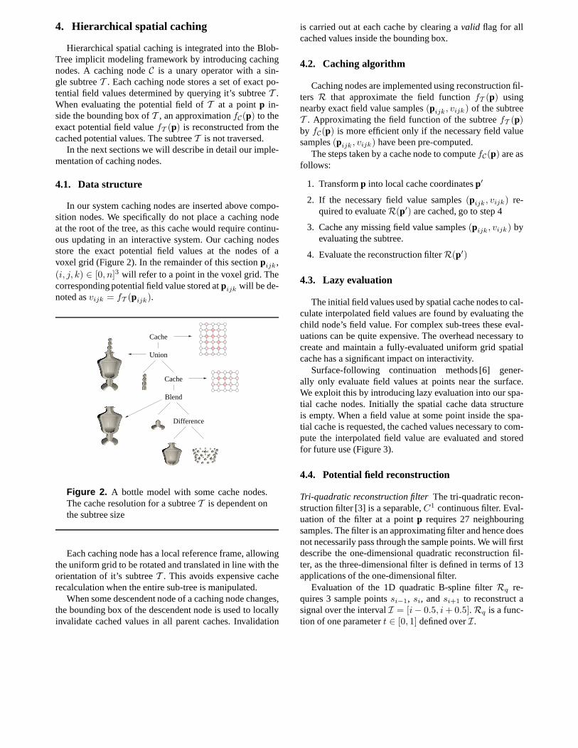
Surface-following continuation methods [6] gener-ally only evaluate field values at points near the surface.We exploit this by introducing lazy evaluation into our spa-tial cache nodes. Initially the spatial cache data structureis empty. When a field value at some point inside the spa-tial cache is requested, the cached values necessary to com-pute the interpolated field value are evaluated and storedfor future use (Figure 3).

4.4. Potential field reconstruction

Tri-quadratic reconstruction filterThe tri-quadratic recon-struction filter [3] is a separable,C1 continuous filter. Eval-uation of the filter at a pointp requires 27 neighbouringsamples. The filter is an approximating filter and hence doesnot necessarily pass through the sample points. We will firstdescribe the one-dimensional quadratic reconstruction fil-ter, as the three-dimensional filter is defined in terms of 13applications of the one-dimensional filter.

Evaluation of the 1D quadratic B-spline filterRq re-quires 3 sample pointssi−1, si, andsi+1 to reconstruct asignal over the intervalI = [i − 0.5, i + 0.5]. Rq is a func-tion of one parametert ∈ [0, 1] defined overI.

Blend

Union

Cacheijk

p

p

T pf ( )ijkBlend

Union

Cache

p

Blend

Union

Cacheijk

p

p

C pijk

p

T pf ( )ijk

f ( )

Figure 3. Lazy evaluation process for three points. The sub-tree is not traversed when evaluating the third point.

We define the 1D quadratic B-spline filterFq as

Rq (si−1, si, si+1, t) =(

si−1 + si+1

2− si

)

t2 + (si − si−1) t +si−1 + si

2

We can now define the tri-quadratic reconstruction fil-ter Rq3 . Evaluation of the filter at a 3D sample point re-quires 27 neighbouring voxels. For a 3D sample pointp, wefind the nearest voxelvijk . The three one-dimensional pa-rametersti, tj , andtk are determined.Rq3(p) is calculatedby repeated applications ofRq, defined in the the follow-ing set of equations.

Rq3(p) = Rq (Rj(k − 1),Rj(k),Rj(k + 1), tk)

Rj(ρ) = Rq (Ri(j − 1, ρ),Ri(j, ρ),Ri(j + 1, ρ), tj)

Ri(φ, ρ) = Rq

(

v(i−1)φρ, viφρ, v(i+1)φρ, ti)

Hereφ andρ are placeholders.Ri(φ, ρ) is an evaluationof Rq in the i direction, andRj(ρ) is an evaluation ofRq

in thej direction.

Reconstruction filter implementationWe reconstruct asmooth scalar value field by applying both reconstruc-tion filters to the potential field values stored in the uniformgrid. We have evaluated both tri-linear and tri-quadratic re-construction filters. Our current system uses tri-linear inter-polation to reconstruct the potential field and tri-quadraticapproximation to reconstruct the field gradients. Wefound this to be the best trade-off between polygoniza-tion time and appearance of surface smoothness.

Tri-linear interpolation is very efficient, requiring only8grid values. However, as shown in [13] the tri-linear filter isonly C0 continuous. This causes significant gradient error,shown in Figure 4.

The tri-quadratic reconstruction filter produces a smoothgradient, however it is significantly more expensive thanthe tri-linear filter and requires more adjacent potential fieldvalue samples. High-frequency details of the original po-tential value field can also be lost due to the approximatingproperty of the filter.

Polygonization using the tri-quadratic filter took approx-imately twice as long as with the tri-linear filter in our eval-uation. However, we found that using tri-linear reconstruc-tion for field values and tri-quadratic reconstruction for gra-dients was only 10% more expensive than a pure tri-linearapproach. The resuling mesh is visually much smoother, asseen in Figure 4.

Figure 4. Trilinear field value and trilinear gradient(a) Trilinear field value and triquadratic gradient (b).

4.5. Cache resolution

The accuracy of the potential field reconstruction is en-tirely dependent on the uniform grid resolution. In ourcurrent implementation the resolution of a uniform gridcaching a subtreeT is dependent on the axis-aligned bound-ing box of the subtree and a user-defined grid resolutionr.Let s denote the longest side of the bounding box ofT . Thesize of each grid cell is then defined as

c = s/r

If some descendent of the cache nodeC is modifed, thebounding box ofT will change. In this case we compute a

new cell sizec′. If the raioc′/c is greater than2 or less than0.5, we destroy the current cache. During the next frame thecache will automatically be re-evaluated by the lazy evalu-ation system. This prevents cache resolution both from get-ting too low, which would result in a coarse approximationof the surface, as well as from getting too high and wast-ing memory.

The effect of varying the grid resolution parameterris demonstrated in Figure 6. In these images we use tri-quadratic reconstruction for both the value and gradient, asit generates smoother surfaces at low cache resolutions. Ex-amining the left hand component of the model is instruc-tive. Even when the grid resolution is only163, the com-ponent is reasonably well-represented for this viewing dis-tance. However,643 is clearly too low a resolution for thebody components. These images indicate that an automaticcache level-of-detail algorithm could reduce both memoryuse and computation time.

One potential issue with caching nodes is a loss of sharpfeatures. The potential value field around several sharp fea-tures is shown in Figure 5. The image pixels are colored bycalculatingsin(11πf(p)) along a plane slice and convert-ing the result to grayscale, with pixels near the iso-value0.5 colored red. At this resolution tri-linear reconstructionis capable of properly reconstructing sharp features that layon voxel edges. Tri-quadratic reconstruction smooths outall sharp features. The reconstruction accuracy improves inboth cases if cache resolution is increased.

(c)(b)(a)

Figure 5. Sharp feature reconstruction using 1283

cache. Tri-linear reconstruction (a), tri-quadratic re-construction (b), and non-cached evaluation (c).

5. Implementation details

Uniform 3D grids can require significant amountsof memory. We store our cached field values in single-

precision floating point, so a 1283 cache requires 8MBof memory. Current hardware limitations prevent stor-ing a significant number of fixed caches at this reso-lution. In addition, the volume that much be cachedcan expand, making a fixed grid data structure undesir-able.

To reduce memory usage we implement our uniform3D grid using a blocked memory scheme. We divide theuniform grid into 8x8x8 blocks of voxels. A uniform gridblock is allocated only when one of the voxels it containsis needed to compute a field value. The blocks are quicklyidentified using a 30-bit hash, using 10 bits per integer gridaxis coordinate. This limits us to 1024 blocks along eachgrid axis, and a total grid size of 80963 voxels.

Continuation methods for polygonizing an implicit sur-face [6] are designed to follow the implicit surface. Mostfield evaluations are near the surface, hence the requiredvoxels. will also be near the surface. In this case our datastructure reduces memory use while still permitting efficientevaluation of the reconstruction filters.

Current workstation processors contain several levels ofhardware memory cache to reduce memory access latency.The traditional static allocation of a large 3D uniform gridcauses frequent cache misses, particularly when accessingadjacent voxels along the z axis. Our blocked allocationscheme potentially increases processor cache coherency,however this effect is difficult to isolate.

Memory requirements can be reduced even further by us-ing an encoding scheme, at the expense of some reconstruc-tion accuracy. The range of potential field values that canoccur in our system is small. Memory usage can be reduced50 to 75 percent by encoding floating point values as one ortwo-byte integers. This technique is slightly more computa-tionally expensive and decreases accuracy, so we do not useit in our evaluation.

6. Results

Cache efficiency is evaluated by comparing polygoniza-tion times between two versions of the same model, onewith cache nodes and one without. We use an optimizedversion of the implicit surface polygonizer described in[5] with the optional cubical decomposition enabled. Whencomputing a mesh vertex on a cube edge,10 bisections areperformed to locate the implicit surface.

The software is compiled with Microsoft Visual Studio.NET 2003 in Release mode with default optimization flags.All timings are performed with an Intel 1.6Ghz Mobile Pen-tium 4 processor with 512MB of RAM.

Figure 6. Varying cache resolution with tri-quadratic value reconstruction. There are three cached components in thismodel - upper body, lower body, and left hand. Cache resolution for each component is varied from left to right 163,323, 643, and 1283.

6.1. Medusa model

We have tested the system with a complex hierarchicalMedusa model. The model is composed of 9490 point prim-itives segmented into 7 major components. The names andprimitive counts are shown in the table below.

Tail Body Chest Left Hand Neck Head Hair

810 840 40 570 20 700 6510

Each major component is modeled as a blend of pointprimitives distributed along a set of splines. All the primi-tives along each individual spline are grouped together intoa single optimized blend node to avoid excessive tree tra-versal.

A caching node with a resolution of1283 voxels wasplaced above each major component in the model tree.We approximate potential field reconstruction accuracy bycomparing reconstructed and exact field values at trianglemesh vertices. Using this method, the error for the medusamodel is estimated to be approximately3% with tri-linearreconstruction. The error is concentrated in high-frequencyregions, particularly the head. We have not devised a globalmeasure of reconstruction accuracy, however it is suspectedthat the global error will be similar to the near-surface er-ror because the cache spacing is uniform.

6.2. Static polygonization time

We compare polygonization times for the Medusa modelwith and without caching nodes. All caches are cleared be-fore each polygonization. Our results are shown in Table 1.

In all cases the cached polygonization contained less than1% more triangles that the non-cached polygonization.

Cubes Cache No Cache Ratio

323 5.77 4.90 0.8×

643 10.34 14.36 1.4×

1283 17.40 51.97 3×

2563 29.23 199.37 6.5×

5123 49.83 809.66 16×

Table 1. Comparison of cached and non-cachedpolygonization times (in seconds) for Medusa modelat different polygonization resolutions.

Polygonization time without caching increases by ap-proximately a factor of 4 when resolution doubles.Polygonization time with caching is initially slower thanwithout because we require8 voxels to compute a sin-gle tri-linear interpolation. Subsequently, polygonizationtime reduces as the cache is populated. The ratio be-tween cached times at consective resolutions decreasesbecause more cached voxels are re-used. At5123 polygo-nizer resolution, approximately33% of all cache voxelshave been evaluated.

We have repeated these tests with a variety of other mod-els constructed from primitives more complex than points,including those shown in Figure 8. Similar results were ob-

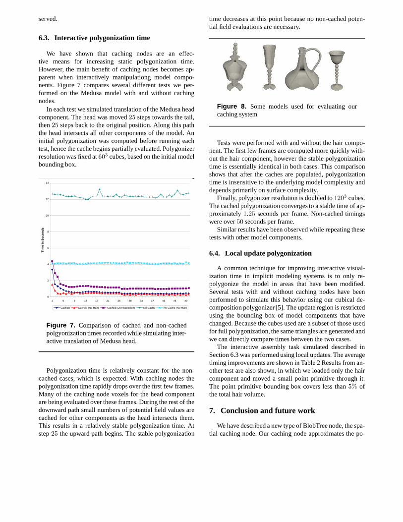
served.

6.3. Interactive polygonization time

We have shown that caching nodes are an effec-tive means for increasing static polygonization time.However, the main benefit of caching nodes becomes ap-parent when interactively manipulationg model compo-nents. Figure 7 compares several different tests we per-formed on the Medusa model with and without cachingnodes.

In each test we simulated translation of the Medusa headcomponent. The head was moved25 steps towards the tail,then25 steps back to the original position. Along this paththe head intersects all other components of the model. Aninitial polygonization was computed before running eachtest, hence the cache begins partially evaluated. Polygonizerresolution was fixed at603 cubes, based on the initial modelbounding box.

0

2

4

6

8

10

12

14

1 5 9 13 17 21 25 29 33 37 41 45 49

Tim

e in

Sec

on

ds

Cached Cached (No Hair) Cached (2x Resolution) No Cache No Cache (No Hair)

Figure 7. Comparison of cached and non-cachedpolgyonization times recorded while simulating inter-active translation of Medusa head.

Polygonization time is relatively constant for the non-cached cases, which is expected. With caching nodes thepolygonization time rapidly drops over the first few frames.Many of the caching node voxels for the head componentare being evaluated over these frames. During the rest of thedownward path small numbers of potential field values arecached for other components as the head intersects them.This results in a relatively stable polygonization time. Atstep25 the upward path begins. The stable polygonization

time decreases at this point because no non-cached poten-tial field evaluations are necessary.

Figure 8. Some models used for evaluating ourcaching system

Tests were performed with and without the hair compo-nent. The first few frames are computed more quickly with-out the hair component, however the stable polygonizationtime is essentially identical in both cases. This comparisonshows that after the caches are populated, polygonizationtime is insensitive to the underlying model complexity anddepends primarily on surface complexity.

Finally, polygonizer resolution is doubled to1203 cubes.The cached polygonization converges to a stable time of ap-proximately1.25 seconds per frame. Non-cached timingswere over50 seconds per frame.

Similar results have been observed while repeating thesetests with other model components.

6.4. Local update polygonization

A common technique for improving interactive visual-ization time in implicit modeling systems is to only re-polygonize the model in areas that have been modified.Several tests with and without caching nodes have beenperformed to simulate this behavior using our cubical de-composition polygonizer [5]. The update region is restrictedusing the bounding box of model components that havechanged. Because the cubes used are a subset of those usedfor full polygonization, the same triangles are generated andwe can directly compare times between the two cases.

The interactive assembly task simulated described inSection 6.3 was performed using local updates. The averagetiming improvements are shown in Table 2 Results from an-other test are also shown, in which we loaded only the haircomponent and moved a small point primitive through it.The point primitive bounding box covers less than5% ofthe total hair volume.

7. Conclusion and future work

We have described a new type of BlobTree node, the spa-tial caching node. Our caching node approximates the po-

Test Cubes Improvement

Head Translation 603 7×

Head Translation 1203 12×

Point / Hair Test 603 30×

Point / Hair Test 1203 47×

Table 2. Comparison of cached and non-cachedpolygonization times for local-update polygonizationtests.Cubescolumn refers to polygonizer resolution,Improvementcolumn shows number of times speed-up with caching nodes.

tential field of a caching node subtree using a set of exactpotential field value samples. The approximation processreduces potential field evaluation complexity for the sub-tree fromO(n) to O(1), wheren refers to the number ofnodes in the subtree.

We implement caching nodes using uniform gridswith subtree-dependent resolution. Our implementa-tion uses tri-linear reconstruction for potential field valuesand tri-quadratic reconstruction for potential field gradi-ents. This combination of reconstruction filters producesvisually smooth meshes suitable for interactive visualisa-tion in an implicit modeling tool. Complex hierarchicalimplicit models created using our interactive model-ing tool are shown in figure 9.

We demonstrate an order-of-magnitude decrease inpolygonization time when inserting caching nodes into acomplex BlobTree model containing over 9000 blendedpoint primitives. The benefit of caching nodes increases sig-nificantly at higher polygonization resolutions. Our analy-sis shows that caching nodes are particularly effectivewhen used in conjunction with local-update polygoniza-tion.

Caching nodes are an effective tool for reducing inter-active polygonization time when using continuation meth-ods. We anticipate that caching nodes will provide a sim-ilar performance benefit with other implicit surface opera-tions, including ray-tracing, collision detection, and otherpolygonization schemes.

There are a variety of avenues for future work on cachingnodes. A primary concern is memory management. Our cur-rent implicit modeling tool requires the model designer tomanage placement of caching nodes. Ideally, an interactivemodeling system would infer appropriate cache placementand resolution based on the designer’s actions.

Our system uses a blocked uniform grid scheme to ob-tain maximum computational efficiency while still main-taining some flexibility. It may be acceptable to trade some

of that efficiency for other parameters, such as increased re-construction accuracy. Alternate spatial data structures, par-ticularly multi-grid methods, may provide this trade-off.

References

[1] B. Araujo and J. Jorge. BlobMaker: Free-Form Modelingwith Variational Implicit Surfaces.Comunicacao ao 12o En-contro Portugues de Computacao Grafica, 2003.

[2] A. Barbier, E. Galin and S. Akkouche. Complex Skeletal Im-plicit Surfaces with Levels of Detail.Proceedings of WSCG,12(4), 35–42, 2004.

[3] L. Barthe, B. Mora, N. Dodgson and M. Sabin. Interactiveimplicit modelling based onC1 reconstruction of regulargrids. International Journal of Shape Modeling, 8(2), 99–117, 2002.

[4] J. Bloomenthal and K. Shoemake. Convlution Surfaces.Computer Graphics, 25(4), 251–256, 1991. Proceedings ofSIGGRAPH ‘91.

[5] J. Bloomenthal. An Implicit Surface Polygonizer.GraphicsGems IV, Academic Press Professional Inc., 324–349, 1994.

[6] J. Bloomenthal (Ed.). Introduction to Implicit Surfaces. Mor-gan Kaufmann, ISBN 1-55860-233-X, 1997.

[7] E. Ferley, M.-P. Cani, J.-D. Gascuel. Practical VolumetricSculpting.The Visual Computer, 16(8), 469–480, 2000.

[8] E. Galin and S. Akkouche. Incremental Polygonization ofImplicit Surfaces,Graphical Models, 62, 19–39, 2000.

[9] S. Akkouche and E. Galin. Adaptive Implicit SurfacePolygonization using Marching Triangles.Computer Graph-ics Forum, 20(2), 67–80, 2001.

[10] S. Frisken, R. Perry, A. Rockwood, T. Jones. Adaptive Sam-pled Distance Fields: A General Representation of Shape forComputer Graphics.Proceedings of ACM SIGGRAPH 2000,249–254, 2000.

[11] S. Hornus, A. Angelidis and M.-P. Cani. Implicit Modelingusing Subdivision-curves.The Visual Computer, 2(3), 94–101, 2003.

[12] O. Karpenko, J. Hughes and R. Raskar. Free-Form Sketch-ing with Variational Implicit Surfaces.Computer GraphicsForum, 21(3), 585–594, 2002.

[13] S. Marschner and R. Lobb. An Evaluation of ReconstructionFilters for Volume Rendering.Proceedings of Visualization1994, 100–107, 1994.

[14] K. Museth, D. Breen, R. Whitaker and A. Barr. Level SetSurface Editing Operators.Proceedings of ACM SIGGRAPH2002, 330–338, 2002.

[15] A. Pasko, V. Adzhiev, A. Sourin and V. Savchenko. Functionrepresentation in geometric modeling: concepts, implemen-tation and applications.The Visual Computer, 11(8), 429–446, 1995.

[16] G. Turk and J. O’Brien. Variational Implicit Surfaces.TechReport GIT-GVU-99-15, Georgia Institute of Technology,May 1999.

[17] B. Walter, G. Drettakis and S. Parker. Interactive Renderingusing the Render Cache.Proceedings of the 10th Eurograph-ics Workshop on Rendering, 10, 235–246, 1999.

[18] A. Witkin and P. Heckbert. Using Particles to Sample andContol Implicit Surfaces.Proceedings of ACM SIGGRAPH1994, 169–277, 1994.

[19] B. Wyvill, A. Guy and E. Galin. Extending the CSG Tree(Warping, Blending and Boolean Operations in an Im-plicit Surface Modeling System).Computer Graphics Fo-rum, 18(2), 149–158, 1999.

Figure 9. Complex hierarchical implicit models created interactively using our system.