Performance and Scalability of PreconditionedConjugate Gradient Methods on Parallel Computers�Anshul Gupta, Vipin Kumar, and Ahmed SamehDepartment of Computer ScienceUniversity of MinnesotaMinneapolis, MN - 55455July 30, 1997AbstractThis paper analyzes the performance and scalability of an iteration of the Preconditioned ConjugateGradient Algorithm on parallel architectures with a variety of interconnection networks, such as the mesh,the hypercube, and that of the CM-5TM y parallel computer. It is shown that for block-tridiagonal matricesresulting from two dimensional �nite di�erence grids, the communication overhead due to vector innerproducts dominates the communication overheads of the remainder of the computation on a large numberof processors. However, with a suitable mapping, the parallel formulation of a PCG iteration is highlyscalable for such matrices on a machine like the CM-5 whose fast control network practically eliminatesthe overheads due to inner product computation. The use of the truncated Incomplete Cholesky (IC)preconditioner can lead to further improvement in scalability on the CM-5 by a constant factor. As aresult, a parallel formulation of the PCG algorithm with IC preconditioner may execute faster than thatwith a simple diagonal preconditioner even if the latter runs faster in a serial implementation. For thematrices resulting from three dimensional �nite di�erence grids, the scalability is quite good on a hypercubeor the CM-5, but not as good on a 2-D mesh architecture. In case of unstructured sparse matrices witha constant number of non-zero elements in each row, the parallel formulation of the PCG iteration isunscalable on any message passing parallel architecture, unless some ordering is applied on the sparsematrix. The parallel system can be made scalable either if, after re-ordering, the non-zero elements of theN �N matrix can be con�ned in a band whose width is O(Ny) for any y < 1, or if the number of non-zeroelements per row increases as Nx for any x > 0. Scalability increases as the number of non-zero elementsper row is increased and/or the width of the band containing these elements is reduced. For unstructuredsparse matrices, the scalability is asymptotically the same for all architectures. Many of these analyticalresults are experimentally veri�ed on the CM-5 parallel computer.�This work was supported by IST/SDIO through the Army Research O�ce grant # 28408-MA-SDI to the Universityof Minnesota and by the University of Minnesota Army High Performance Computing Research Center under contract# DAAL03-89-C-0038.yCM-5 is a trademark of the Thinking Machines Corporation.1

1 IntroductionSolving large sparse systems of linear equations is an integral part of mathematical and scienti�ccomputing and �nds application in a variety of �elds such as uid dynamics, structural analysis,circuit theory, power system analysis, surveying, and atmospheric modeling. With the availability oflarge-scale parallel computers, iterative methods such as the Conjugate Gradient method for solvingsuch systems are becoming increasingly appealing, as they can be parallelized with much greaterease than direct methods. As a result there has been a great deal of interest in implementing theConjugate Gradient algorithm on parallel computers [1, 2, 12, 14, 16, 21, 25, 29, 30]. In this paper,we study performance and scalability of parallel formulations of an iteration of the PreconditionedConjugate Gradient (PCG) algorithm [6] for solving large sparse linear systems of equations of theform A x = b, where A is a symmetric positive de�nite matrix. Although, we speci�cally deal withthe Preconditioned CG algorithm only, the analysis of the diagonal preconditioner case applies tothe non-preconditioned method also. In fact the results of this paper can be adapted to a number ofiterative methods that use matrix-vector multiplication and vector inner product calculation as thebasic operations in each iteration.The scalability of a parallel algorithm on a parallel architecture is a measure of its capability toe�ectively utilize an increasing number of processors. It is important to analyze the scalability of aparallel system because one can often reach very misleading conclusions regarding the performanceof a large parallel system by simply extrapolating the performance of a similar smaller system. Manydi�erent measures have been developed to study the scalability of parallel algorithms and architectures[3, 7, 10, 15, 19, 22, 28, 32, 33]. In this paper, we use the isoe�ciency metric [18, 7, 19] to study thescalability of an iteration of the PCG algorithm on some important architectures. The isoe�ciencyfunction of a combination of a parallel algorithm and a parallel architecture relates the problem sizeto the number of processors necessary for an increase in speedup in proportion to the number ofprocessors. Isoe�ciency analysis has been found to be very useful in characterizing the scalabilityof a variety of parallel algorithms [9, 8, 13, 17, 23, 27, 26, 31]. An important feature of isoe�ciencyanalysis is that it succinctly captures the e�ects of characteristics of the parallel algorithm as well asthe parallel architecture on which it is implemented, in a single expression.The scalability and the overall performance of an iteration of the PCG schemes on a parallel com-puter depends on - (i) hardware parameters such as the interconnection network and communicationand computation speeds, (ii) the characteristics of the matrix A such as its degree of sparsity and thearrangement of the non-zero elements within it, and (iii) the use and the choice of preconditioners.This paper analyzes the impact of all three types of factors on the scalability of a PCG iterationon parallel architectures with parallel interconnection networks such as mesh, hypercube and that ofTMC's CM-5. Two di�erent kinds of matrices are considered. First we analyze the scalability of aPCG iteration on block-tridiagonal matrices resulting from the discretization of a 2-dimensional self-adjoint elliptic partial di�erential equation via �nite di�erences using natural ordering of grid points.Two commonly used schemes for mapping the data onto the processors are compared, and one isshown to be strictly better than the other. We also consider the use of two di�erent types of pre-conditioners - a diagonal preconditioner, and one resulting from the truncated Incomplete Choleskyfactorization of the matrix of coe�cients. The truncated version of Incomplete Cholesky factorizationreplaces triangular solvers by matrix-vector products, which is henceforth referred to as IC factoriza-2

tion. The results are then extended to the matrices resulting from three dimensional �nite di�erencegrids. The second type of matrices that are studied are unstructured sparse symmetric positive de�-nite matrices. The analytical results are veri�ed through extensive experiments on the CM-5 parallelcomputer. This analysis helps in answering a number of questions, such as -Given a problem and a parallel machine, what kind of e�ciencies are expected?How should the problem size be increased with the number of processors to maintain a certaine�ciency?Which feature of the hardware should be improved for maximum returns in terms of performanceper unit cost?How does the mapping of the matrix of coe�cients onto the processors a�ect the performanceand scalability of a PCG iteration?How does the truncated Incomplete Cholesky (IC) preconditioner compare with a simple diag-onal preconditioner in terms of performance on a parallel computer?What kind of improvement in scalability can be achieved by re-ordering the sparse matrix?Which parts of the algorithm dominate in terms of communication overheads and hence deter-mine the overall parallel speedup and e�ciency?The organization of this paper is as follows. Section 2 de�nes the terms frequently used in thepaper. Section 3 describes the data communication model for the parallel architectures considered foranalysis in this paper. Section 4 gives an overview of the isoe�ciency metric of scalability. The serialPCG algorithm is described in Section 5. The scalability analysis of a PCG iteration on di�erentparallel architectures is presented in Sections 6 and 7 for block-tridiagonal matrices and in Section 8for unstructured sparse matrices. The experimental results are presented in Section 9, and Section10 contains concluding remarks.2 TerminologyIn this section, we introduce the terminology that shall be followed in the rest of the paper.Parallel System: The combination of a parallel algorithm and the parallel architecture on whichit is implemented.Number of Processors, p: The number of homogeneous processing units in the parallel computerthat cooperate to solve a problem.Problem Size, W : The time taken by an optimal (or the best known) sequential algorithm to solvethe given problem on a single processor. For example, for multiplying an N � N matrix withan N � 1 vector, W = O(N2). 3

Parallel Execution Time, TP : The time taken by p processors to solve a problem. For a givenparallel system, TP is a function of the problem size and the number of processors.Parallel Speedup, S: The ratio of W to TP .Total Parallel Overhead, To: The sum total of all overheads incurred by all the processors duringthe parallel execution of the algorithm. It includes communication costs, non-essential work andidle time due to synchronization and serial components of the algorithm. For a given parallelsystem, To is usually a function of the problem size and the number of processors and is oftenwritten as To(W;p). Thus To(W;p) = pTP �W .E�ciency, E: The ratio of S to p. Hence, E =W=pTP = 1=(1 + ToW ).3 Parallel architectures and message passing costsIn this paper we consider parallel architectures with the following interconnection networks: mesh,hypercube, and that of the CM-5 parallel computer. We assume that in all these architectures,cut-through routing is used for message passing. The time required for the complete transfer of amessage of size q between two processors that are d connections away; (i.e., there are d�1 processorsin between) is given by ts + th(d � 1) + twq, where ts is the message startup time, th (called per-hoptime) is the time delay for a message fragment to travel from one node to an immediate neighbor,and tw (called per-word time) is equal to 1B where B is the bandwidth of the communication channelbetween the processors in words/second.The analytical results presented in the paper are veri�ed through experiments on the CM-5 parallelcomputer. On CM-5, the fat-tree [20] like communication network provides (almost) simultaneouspaths for communication between all pairs of processors. The length of these paths may vary from2 to 2 log p, if the distance between two switches or a processor and a switch is considered to be oneunit [20]. Hence, the cost of passing a message of size q between any pair of processors on the CM-5is approximately ts + twq + th �O(log p). An additional feature of this machine is that it has a fastcontrol network which can perform certain global operations like scan and reduce in a small constanttime. This feature of the CM-5 makes the overheads of certain operations, like computing the innerproduct of two vectors, almost negligible compared to the communication overheads involved in therest of the parallel operations in the CG algorithm.On most practical parallel computers with cut-through routing, the value of th is fairly small. Inthis paper, we will omit the th term from any expression in which the coe�cient of th is dominatedby coe�cients of tw or ts.4 The isoe�ciency metric of scalabilityIt is well known that given a parallel architecture and a problem instance of a �xed size, the speedupof a parallel algorithm does not continue to increase with increasing number of processors but tends tosaturate or peak at a certain value. For a �xed problem size, the speedup saturates either because theoverheads grow with increasing number of processors or because the number of processors eventually4

exceeds the degree of concurrency inherent in the algorithm. For a variety of parallel systems, givenany number of processors p, speedup arbitrarily close to p can be obtained by simply executing theparallel algorithm on big enough problem instances (e.g., [18, 7, 11, 32]). The ease with which aparallel algorithm can achieve speedups proportional to p on a parallel architecture can serve as ameasure of the scalability of the parallel system.The isoe�ciency function [18, 7] is one such metric of scalability which is a measure of an algo-rithm's capability to e�ectively utilize an increasing number of processors on a parallel architecture.The isoe�ciency function of a combination of a parallel algorithm and a parallel architecture relatesthe problem size to the number of processors necessary to maintain a �xed e�ciency or to deliverspeedups increasing proportionally with increasing number of processors. The e�ciency of a parallelsystem is given by E = WW+To(W;p) . If a parallel system is used to solve a problem instance of a �xedsize W , then the e�ciency decreases as p increases. The reason is that the total overhead To(W;p)increases with p. For many parallel systems, for a �xed p, if the problem size W is increased, thenthe e�ciency increases because for a given p, To(W;p) grows slower than O(W ). For these parallelsystems, the e�ciency can be maintained at a desired value (between 0 and 1) for increasing p, pro-vided W is also increased. We call such systems scalable parallel systems. Note that for a givenparallel algorithm, for di�erent parallel architectures, W may have to increase at di�erent rates withrespect to p in order to maintain a �xed e�ciency. For example, in some cases, W might need togrow exponentially with respect to p to keep the e�ciency from dropping as p is increased. Such aparallel system is poorly scalable because it would be di�cult to obtain good speedups for a largenumber of processors, unless the size of the problem being solved is enormously large. On the otherhand, if W needs to grow only linearly with respect to p, then the parallel system is highly scalableand can easily deliver speedups increasing linearly with respect to the number of processors for rea-sonably increasing problem sizes. The isoe�ciency functions of several common parallel systems arepolynomial functions of p; i.e., they are O(px), where x � 1. A small power of p in the isoe�ciencyfunction indicates a high scalability.If a parallel system incurs a total overhead of To(W;p), where p is the number of processorsin the parallel ensemble and W is the problem size, then the e�ciency of the system is given byE = 11+To(W;p)W . In order to maintain a �xed e�ciency, W should be proportional to To(W;p) or thefollowing relation must be satis�ed: W = eTo(W;p); (1)where e = E1�E is a constant depending on the e�ciency to be maintained. Equation (1) is the centralrelation that is used to determine the isoe�ciency function of a parallel system. This is accomplishedby abstracting W as a function of p through algebraic manipulations on Equation (1). If the problemsize needs to grow as fast as fE(p) to maintain an e�ciency E, then fE(p) is de�ned as the isoe�ciencyfunction of the parallel system for e�ciency E.An important feature of isoe�ciency analysis is that in a single expression, it succinctly capturesthe e�ects of characteristics of the parallel algorithm as well as those of the parallel architectureon which it is implemented. By performing isoe�ciency analysis, one can test the performanceof a parallel program on a few processors, and then predict its performance on a larger numberof processors. The utility of the isoe�ciency analysis is not limited to predicting the impact onperformance of an increasing number of processors. It can also be used to study the behavior of a5

parallel system with respect to changes in other hardware related parameters such as the speed ofthe processors and the data communication channels.5 The serial PCG algorithm1. begin2. i := 0; x0 := 0; r0 := b; �0 := jjr0jj22;3. while (p�i > �jjr0jj2) and (i < imax) do4. begin5. Solve M zi = ri;6. i := rTi zi;7. i := i+ 1;8. if (i = 1) p1 := z09. else begin10. �i := i�1= i�2;11. pi := zi�1 + �ipi�1;12. end;13. wi := A pi;14. �i := i�1/pTi wi;15. xi := xi�1 + �ipi;16. ri := ri�1 � �iwi;17. �i := jjrijj22;18. end; f while g19. x := xi;20. end. Figure 1: The Preconditioned Conjugate Gradient algorithm.Figure 1 illustrates the PCG algorithm [6] for solving a linear system of equations A x = b, where Ais a sparse symmetric positive de�nite matrix. The PCG algorithm performs a few basic operations ineach iteration. These are matrix-vector multiplication, vector inner product calculation, scalar-vectormultiplication, vector addition and solution of a linear systemM z = r. HereM is the preconditionermatrix, usually derived from A using certain techniques. In this paper, we will consider two kinds ofpreconditioner matrices M - (i) when M is chosen to be a diagonal matrix, usually derived from theprincipal diagonal of A, and (ii) when M is obtained through a truncated Incomplete Cholesky (IC)factorization [14, 29] of A. In the following subsections, we determine the serial execution time foreach iteration of the PCG algorithm with both preconditioners.6

5.1 Diagonal preconditionerDuring a PCG iteration for solving a system of N equations, the serial complexity of computing thevector inner product, scalar-vector multiplication and vector addition is O(N). If M is a diagonalmatrix, the complexity of solving M z = r is also O(N). If there are m non-zero elements in eachrow of the sparse matrix A, then the matrix-vector multiplication of a CG iteration can be performedin O(mN) time by using a suitable scheme for storing A. Thus, with the diagonal preconditioner,each CG iteration involves a few steps of O(N) complexity and one step of O(mN) complexity. As aresult, the serial execution time for one iteration of the PCG algorithm with a diagonal preconditionercan be expressed as follows: W = c1N + c2mN (2)Here c1 and c2 are constants depending upon the oating point speed of the computer and m is thenumber non-zero elements in each row of the sparse matrix.5.2 The IC preconditionerIn this section, we only consider the case when A is a block-tridiagonal matrix of dimension Nresulting from the discretization of a 2-dimensional self-adjoint elliptic partial di�erential equationvia �nite di�erences using natural ordering of grid points. Besides the principal diagonal, the matrixA has two diagonals on each side of the principal diagonal at distances of 1 and pN from it. Clearly,all the vector operations can be performed in O(N) time. The matrix-vector multiplication operationtakes time proportional to 5N . When M is an IC preconditioner, the structure of M is identical tothat of A.A method for solving M z = r, originally proposed for vector machines [29], is brie y describedbelow. A detailed description of the same can be found in [18]. As shown in Section 6, this methodis perfectly parallelizable on CM-5 and other architectures ranging from mesh to hypercube. In fact,this method leads to a parallel formulation of the PCG algorithm that is somewhat more scalable ande�cient (in terms of processor utilization) than a formulation using a simple diagonal preconditioner.The matrix M can be written as M = (I - L)D(I - LT ), where D is a diagonal matrix and L isa strictly lower triangular matrix with two diagonals corresponding to the two lower diagonals of M.Thus, the system Mz = r may be solved by the following steps:solve (I - L)u = rsolve Dv = usolve (I - LT )z = vSince L is strictly lower triangular (i.e., LN = 0), u and z may be written as u = �N�1i=0 Lir and z= �N�1i=0 (Li)Tv. These series may be truncated to (k+1) terms where k � N becauseM is diagonallydominant [14, 29]. In our formulation, we form the matrix ~L = (I + L + L2 + ... + Lk) explicitly.Thus, solving Mz = r is equivalent to(i) u � ~Lr(ii) v � D�1u(iii) z � ~LTv 7

PPPq����9

����(5,5)

(0,5)(0,0).......

. . ..............

...

.........

.P(2;2)P(1;2)P(2;1)P(1;1)P(2;0)P(1;0) P(0;2)P(0;1)P(0;0)

Figure 2: Partitioning a �nite di�erence grid on a processor mesh.The number of diagonals in the matrix ~L is equal to (k+1)(k+2)2 . These diagonals are distributedin k + 1 clusters at distances of pN from each other. The �rst cluster, which includes the principaldiagonal, has k + 1 diagonals, and then the number of diagonals in each cluster decreases by one.The last cluster has only one diagonal which is at a distance of kpN from the principal diagonal.Thus solving the system M z = r, in case of the IC preconditioner, is equivalent to performingone vector division (step (ii)) and two matrix-vector multiplications (steps (i) and (iii)), where eachmatrix has (k+1)(k+2)2 diagonals. Hence the complexity of solvingM z = r for this case is proportionalto (k + 1)(k + 2)N and the serial execution time of one complete iteration is given by the followingequation: W = (c1 + (5 + (k + 1)(k + 2))c2)�NHere c1 and c2 are constants depending upon the oating point speed of the computer. The aboveequation can be written compactly as follows by putting �(k) = c1 + c2(5 + (k + 1)(k + 2)).W = �(k)N (3)6 Scalability analysis: block-tridiagonal matricesIn this section we consider the parallel formulation of the PCG algorithm with block-tridiagonal matrixof coe�cients resulting from a square two dimensional �nite di�erence grid with natural ordering ofgrid points. Each point on the grid contributes one equation to the system A x = b; i.e., one rowof matrix A and one element of the vector b.8

6.1 The parallel formulationThe points on the �nite di�erence grid can be partitioned among the processors of a mesh connectedparallel computer as shown in Figure 2. Since a mesh can be mapped onto a hypercube or a fullyconnected network, a mapping similar to the one shown in Figure 2 will work for these architecturesas well. Let the p processors be numbered from P(0;0) to P(pp�1;pp�1). If the N points of the gridare indexed from [0; 0] to [pN � 1;pN � 1], then processor P(i;j) stores a square subsection of thegrid with row indices varying from [ipN=p] to [(i + 1)pN=p � 1] and column indices varying from[jpN=p] to [(j + 1)pN=p� 1]. If the grid points are ordered naturally, point (q; r) is responsible forrow number [qpN + r] of matrix A and the element with index [qpN + r] of the vector b. Hence,once the grid points are assigned to the processors, it is easy to determine the rows of matrix A andthe elements of vector b that belong to each processor.In the PCG algorithm, the scalar-vector multiplication and vector addition operations do notinvolve any communication overhead, as all the required data is locally available on each processorand the results are stored locally as well. If the diagonal preconditioner is used, then even solvingthe system M z = r does not require any data communication because the resultant vector z can beobtained by simply dividing each element of r by the corresponding diagonal element of M, both ofwhich are locally available on each processor. Thus, the operations that involve any communicationoverheads are computation of inner products, matrix-vector multiplication, and, in case of the ICpreconditioner, solving the system M z = r.In the computation of the inner product of two vectors, the corresponding elements of each vectorare multiplied locally and these products are summed up. The value of the inner product is the sumof these partial sums located at each processor. The data communication required to perform thisstep involves adding all the partial sums and distributing the resulting value to each processor.In order to perform parallel matrix-vector multiplication involving the block-tridiagonal matrix,each processor has to acquire the vector elements corresponding to the column numbers of all thematrix elements it stores. It can be seen from Figure 2 that each processor needs to exchangeinformation corresponding to its qNp boundary points with each of its four neighboring processors.After this communication step, each processor gets all the elements of the vector it needs to multiplywith all the matrix elements it stores. Now the multiplications are performed and the resultantproducts are summed and stored locally on each processor.A method for solving M z = r for the IC preconditioner M has been described in Section 5.2.This computation involves multiplication of a vector with a lower triangular matrix ~L and an uppertriangular matrix ~LT , where each triangular matrix has (k+1)(k+2)2 diagonals arranged in the fashiondescribed in Section 5.2. If the scheme of partitioningA among the processors (every processor storesqNp clusters ofqNp matrix rows each) is extended to ~L and ~LT , then it can be shown that forqNp > kthe data communication for performing these matrix-vector multiplications requires each processorin the mesh to send kqNp vector elements to its immediate north, east, south and west neighbors.6.2 Communication overheadsIn this section we determine the overall overhead due to parallel processing in a PCG iteration.As discussed in the previous subsection, the operations that incur communication overheads are9

computation of inner products, matrix-vector multiplication and solving the system M z = r. Letthese three components of To be T Inner�Prodo , TMatrix�V ectoro , and TPC�solveo , respectively. In order tocompute each component of To, �rst we compute the time spent by each processor in performing datacommunication for the operation in question. The product of this time with p gives the total timespent by all the processors in performing this operation and To is the sum of each of these individualcomponents.6.2.1 Overhead in computing the inner productsThe summation of p partial sums (one located at each processor) can be performed through recursivedoubling in (ts+ tw) log p time on a hypercube, and in (ts+ tw) log p+ thpp time on a two dimensionalmesh. It takes the same amount of time to broadcast the �nal result to each processor. On amachine like the CM-5, such operations (known as reduction operations) are performed by the controlnetwork in a small constant time which can be ignored in comparison with the overhead incurred inother parts of the algorithm, such as, matrix-vector multiplication. The following equations give theexpressions for the total overhead for each iteration over all the processors for computing the threeinner products (lines 6, 14 and 17 in Figure 1) on di�erent architectures. In these equations tw isignored in comparison with ts as the latter is much larger in most practical machines.T Inner�Prodo � 6(ts log p+ thpp)� p (2�D mesh) (4)T Inner�Prodo � 6ts log p� p (Hypercube) (5)T Inner�Prodo � 0 (CM � 5) (6)6.2.2 Overhead due to matrix-vector multiplicationDuring matrix-vector multiplication, each processor needs to exchange vector elements correspondingto its boundary grid points with each of its four neighboring processors. This can be done in 4ts +4twqNp time on a mesh, hypercube or a virtually fully connected network like that of the CM-5. Thetotal overhead for this step is given by the following equation:TMatrix�V ectoro = 4(ts + twsNp )� p (7)6.2.3 Overhead in solving M z = rIf a simple diagonal preconditioner is used, then this step does not require any communication. Forthe case of the IC preconditioner, as discussed in Section 6.1, the communication pattern for thisstep is identical to that for matrix-vector multiplication, except that kqNp vector elements are nowexchanged at each processor boundary. The required expression for the overall overhead for this stepis as follows.TPC�solveo = 0 (diagonal preconditioner) (8)10

TPC�solveo = 4(ts + twksNp )� p (IC preconditioner) (9)6.2.4 Total overheadNow, having computed each of its components, we can write the expressions for the overall To us-ing equations (4) to (9). The following equations give the required approximate expressions (afterdropping the insigni�cant terms, if any) for To.� The CM-5To = 4(tsp+ twppN) (diagonal preconditioner) (10)To = 4(2tsp+ tw(k + 1)ppN) (IC preconditioner) (11)� HypercubeTo = 6tsp log p+ 4twppN (diagonal preconditioner) (12)To = 6tsp log p+ 4(k + 1)twppN (IC preconditioner) (13)� MeshTo = 6tsp log p+ 4twppN + 6thppp (diagonal preconditioner) (14)To = 6tsp log p+ 4(k + 1)twppN + 6thppp (IC preconditioner) (15)6.3 Isoe�ciency analysisSince we perform the scalability analysis with respect to one PCG iteration, the problem size W willbe considered to be O(N) and we will study the rate at which N needs to grow with p for a �xede�ciency as a measure of scalability. If To(W;P ) is the total overhead, the e�ciency E is given byWW+To(W;p) . Clearly, for a given N , if p increases, then E will decrease because To(W;p) increases withp. On the other hand, if N increases, then E increases because the rate of increase of To is slowerthan that of W for a scalable algorithm. The isoe�ciency function for a certain e�ciency E can beobtained by equating W with E1�ETo (Equation (1)) and then solving this equation to determine Nas a function of p. In our parallel formulation, To has a number of di�erent terms due to ts, tw, th,etc. When there are multiple terms of di�erent orders of magnitude with respect to p and N in Wor To, it is often impossible to obtain the isoe�ciency function as a closed form function of p. For aparallel algorithm-architecture combination, as p andW increase, e�ciency is guaranteed not to dropif none of the terms of To grows faster than W . Therefore, if To has multiple terms, we balance Wagainst each individual term of To to compute the respective isoe�ciency function. The component ofTo that requires the problem size to grow at the fastest rate with respect to p determines the overallasymptotic isoe�ciency function of the entire computation.11

6.3.1 Diagonal preconditionerSince the number of elements per row (m) in the matrix of coe�cients is �ve, from Equation (2), weobtain the following expression for W : W = N(c1 + 5c2) (16)Now we will use Equations (10), (12), (14) and (16) to compute the isoe�ciency functions for thecase of diagonal preconditioner on di�erent architectures.� The CM-5According to Equation (1), in order to determine the isoe�ciency term due to ts, W has to beproportional to 4etsp (see Equation (10)), where e = E1�E and E is the desired e�ciency thathas to be maintained. Therefore, N(c1 + 5c2) / 4etsp=> N / p 4etsc1 + 5c2 (17)The term due to tw in To is 4twppN (see Equation (10)) and the associated isoe�ciency con-dition is determined as follows: N(c1 + 5c2) / 4etwppN=> pN / pp 4etwc1 + 5c2=> N / p( 4etwc1 + 5c2 )2 (18)According to both Equations (17) and (18), the overall isoe�ciency function for the PCGalgorithm with a simple diagonal preconditioner is O(p); i.e, it is a highly scalable parallelsystem which requires only a linear growth of problem size with respect to p to maintain acertain e�ciency.� HypercubeSince the terms due to tw are identical in the overhead functions for both the hypercube and theCM-5 architectures, the isoe�ciency condition resulting from tw is still determined by Equation(18). The term associated with ts yields the following isoe�ciency function:=> N / 6etsc1 + 5c2 p log p (19)Since Equation (19) suggests a higher growth rate for the problem size with respect to p tomaintain a �xed E, it determines the overall isoe�ciency function which is O(p log p). Also, tshas a higher impact on the e�ciency on a hypercube than on the CM-5.12

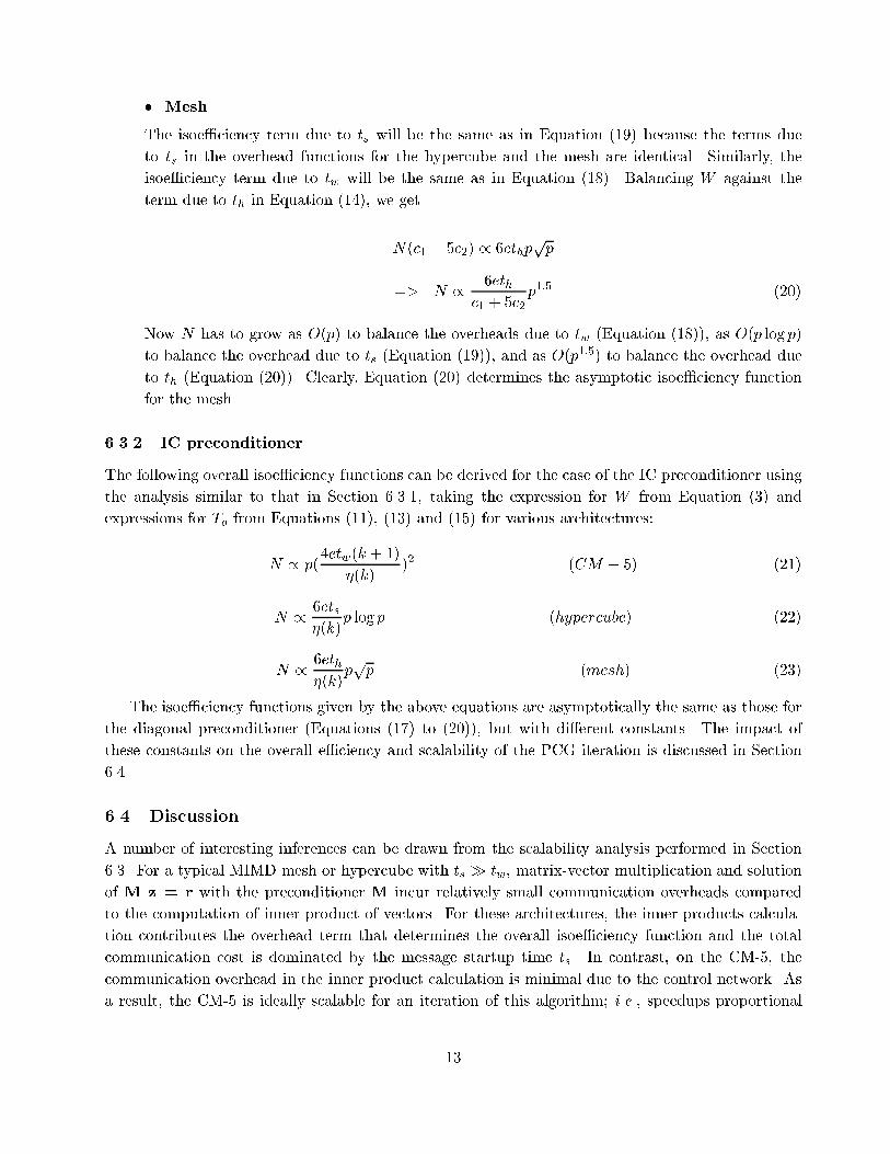
� MeshThe isoe�ciency term due to ts will be the same as in Equation (19) because the terms dueto ts in the overhead functions for the hypercube and the mesh are identical. Similarly, theisoe�ciency term due to tw will be the same as in Equation (18). Balancing W against theterm due to th in Equation (14), we getN(c1 + 5c2) / 6ethppp=> N / 6ethc1 + 5c2 p1:5 (20)Now N has to grow as O(p) to balance the overheads due to tw (Equation (18)), as O(p log p)to balance the overhead due to ts (Equation (19)), and as O(p1:5) to balance the overhead dueto th (Equation (20)). Clearly, Equation (20) determines the asymptotic isoe�ciency functionfor the mesh.6.3.2 IC preconditionerThe following overall isoe�ciency functions can be derived for the case of the IC preconditioner usingthe analysis similar to that in Section 6.3.1, taking the expression for W from Equation (3) andexpressions for To from Equations (11), (13) and (15) for various architectures:N / p(4etw(k + 1)�(k) )2 (CM � 5) (21)N / 6ets�(k)p log p (hypercube) (22)N / 6eth�(k)ppp (mesh) (23)The isoe�ciency functions given by the above equations are asymptotically the same as those forthe diagonal preconditioner (Equations (17) to (20)), but with di�erent constants. The impact ofthese constants on the overall e�ciency and scalability of the PCG iteration is discussed in Section6.4.6.4 DiscussionA number of interesting inferences can be drawn from the scalability analysis performed in Section6.3. For a typical MIMD mesh or hypercube with ts � tw, matrix-vector multiplication and solutionof M z = r with the preconditioner M incur relatively small communication overheads comparedto the computation of inner-product of vectors. For these architectures, the inner-products calcula-tion contributes the overhead term that determines the overall isoe�ciency function and the totalcommunication cost is dominated by the message startup time ts. In contrast, on the CM-5, thecommunication overhead in the inner product calculation is minimal due to the control network. Asa result, the CM-5 is ideally scalable for an iteration of this algorithm; i.e., speedups proportional13

020000400006000080000100000120000140000160000180000

0 100 200 300 400 500 600"N

p!

tw = 1tw = 4tw = 16

Figure 3: Isoe�ciency curves for E = 0:5 with a �xed processor speed and di�erent values of channelbandwidth.to the number of processors can be obtained by simply increasing N linearly with p. Equivalently,bigger instances of problems can be solved in a �xed given time by using linearly increasing numberof processors. In the absence of the control network, even on the CM-5 the overhead due to messagestartup time in the inner product computation would have dominated and the isoe�ciency functionof the PCG algorithm would have been greater than O(p). Thus, for this application, the controlnetwork is highly useful.There are certain iterative schemes, like the Jacobi method [6], that require inner product calcula-tion only for the purpose of performing a convergence check. In such schemes, the parallel formulationcan be made almost linearly scalable even on mesh and hypercube architectures by performing theconvergence check once in a few iterations. For instance, the isoe�ciency function for the Jacobimethod on a hypercube is O(p log p). If the convergence check is performed once every log p itera-tions, the amortized overhead due to inner product calculation will be O(p) in each iteration, insteadof O(p log p) and the isoe�ciency function of the modi�ed scheme will be O(p). Similarly, perform-ing the convergence check once in every pp iterations on a mesh architecture will result in linearscalability.Equations (17) and (18) suggest that the PCG algorithm is highly scalable on a CM-5 type archi-tecture and a linear increase in problem size with respect to the number of processors is su�cient tomaintain a �xed e�ciency. However, we would like to point out as to how hardware related param-eters other than the number of processors a�ect the isoe�ciency function. According to Equation(18), N needs to grow in proportion to the square of the ratio of tw to the unit computation timeon a processor. According to Equation (17), N needs to grow in proportion to the ratio of ts tothe unit computation time. Thus isoe�ciency is also a function of the ratio of communication and14

020000400006000080000100000120000140000160000180000

0 100 200 300 400 500 600"N

p!

ts = 5ts = 20ts = 80

Figure 4: Isoe�ciency curves for E = 0:5 with a �xed processor speed and di�erent values of messagestartup time.computation speeds. Figure 3 shows theoretical isoe�ciency curves for di�erent values of tw for ahypothetical machine with �xed processor speed ((c1+5c2) = 2 microseconds1) and message startuptime (ts = 20 microseconds). Figure 4 shows isoe�ciency curves for di�erent values of ts for thesame processor speed with tw = 4 microseconds. These curves show that the isoe�ciency functionis much more sensitive to changes in tw than ts. Note that ts and tw are normalized with respect toCPU speed. Hence, e�ectively tw could go up if either the CPU speed increases or inter-processorcommunication bandwidth decreases. Figure 3 suggests that it is very important to have a balancebetween the speed of the processors and the bandwidth of the communication channels, otherwisegood e�ciencies will be hard to obtain; i.e., very large problems will be required.Apart from the computation and communication related constants, isoe�ciency is also a functionof the e�ciency that is desired to be maintained. N needs to grow in proportion to ( E1�E )2 in orderto balance the useful computation W with the overhead due to tw (Equation (18)) and in proportionto E1�E to balance the overhead due to ts (Equation (17)). Figure 5 graphically illustrate the impactof desired e�ciency on the scalability of a PCG iteration. The �gure shows that as higher andhigher e�ciencies are desired, it becomes increasingly di�cult to obtain them. An improvement inthe e�ciency from 0.3 to 0.5 takes little e�ort, but it takes substantially larger problem sizes for asimilar increase in e�ciency from 0.7 to 0.9. The constant ( etwc1+5c2 )2 in Equation (18) indicates thata better balance between communication channel bandwidth and the processor speed will reduce theimpact of increasing the e�ciency on the rate of growth of problem size and higher e�ciencies willbe obtained more readily.1This corresponds to a throughput of roughly 10 MFLOPS. On a fully con�gured CM-5 with vector units, a through-put of this order can be achieved very easily. 15

020000400006000080000100000120000140000160000180000

0 100 200 300 400 500 600"N

p!

E = 0.3E = 0.5E = 0.7E = 0.9

Figure 5: Isoe�ciency curves for di�erent e�ciencies with ts = 20 and tw = 4.The isoe�ciency functions for the case of the IC preconditioner for di�erent architectures givenby Equations (21) to (22) are of the same order of magnitude as those for the case of the diagonalpreconditioner given by Equations (17) to (20). However, the constants associated with the isoe�-ciency functions for the IC preconditioner are smaller due to the presence of �(k) in the denominatorwhich is c1 + 5c2 + (k + 1)(k + 2)c2. As a result, the rate at which the problem size should increaseto maintain a particular e�ciency will be asymptotically the same for both preconditioners, but forthe IC preconditioner the same e�ciency can be realized for a smaller problem size than in the caseof the diagonal preconditioner. Also, for given p and N , the parallel implementation with the ICpreconditioner will yield a higher e�ciency and speedup than one with the diagonal preconditioner.Thus, if enough processors are used, a parallel implementation with the IC preconditioner may ex-ecute faster than one with a simple diagonal preconditioner even if the latter was faster in a serialimplementation. The reason is that the number of iterations required to obtain a residual whosenorm satis�es a given constraint does not increase with the number of processors used. However, thee�ciency of execution of each iteration will drop more rapidly in case of the diagonal preconditionerthat in case of the IC preconditioner as the number of processors are increased.It can be shown that the scope of the results of this section is not limited to the type of block-tridiagonal matrices described in Section 5.2 only. The results hold for all symmetric block-tridiagonalmatrices where the distance of the two outer diagonals from the principal diagonal is N r (0 < r <1). Such a matrix will result from a rectangular N r � N1�r �nite di�erence grid with naturalordering of grid points. Similar scalability results can also be derived for matrices resulting fromthree dimensional �nite di�erence grids. These matrices have seven diagonals and the scalabilityof the parallel formulations of an iteration of the PCG algorithm on a hypercube or the CM-5 isthe same as in case of block-tridiagonal matrices. However, for the mesh architecture, the results16

?6 .......................................

..............................................................................................................................................................................................

.....................................

Vector bMatrix AN

Pp�1----P2P1P0

Figure 6: A simple mapping scheme for the block-tridiagonal matrix.will be di�erent. On a two dimensional mesh of processors, the isoe�ciency due to matrix-vectormultiplication will be O(p3=2) for the matrices resulting from 3-D �nite di�erence grids. Thus, unlikethe block-tridiagonal case, here the overheads due to both matrix vector multiplication and inner-product computation are equally dominant on a mesh.7 An alternate mapping for the block-tridiagonal case and its im-pact on scalabilityA scheme for mapping the matrix of coe�cients and the vectors onto the processors has been presentedin Section 6.1. In this section, we describe a di�erent mapping and analyze its scalability. Given thematrix of coe�cients A and the vector b, this mapping is fairly straightforward and has often beenused in parallel implementations of the PCG algorithm due to its simplicity [16, 2, 21, 14]. Herewe will compare this mapping with the one discussed in Section 6.1 in the context of a CM-5 typearchitecture.According to this scheme, the matrix A and the vector b are partitioned among p processorsas shown in Figure 6. The rows and the columns of the matrix and the elements of the vector arenumbered from 0 to N � 1. The diagonal storage scheme is the natural choice for storing the sparsematrix in this case. There are N elements in the principal diagonal and they are indexed from [0] to[N � 1]. The two diagonals in the upper triangular part have N � 1 and N �pN elements indexedfrom [0] to [N�2] and from [0] to [N�pN�1] respectively. The two diagonals in the lower triangularpart of A have the same lengths as their upper triangular counterparts. These are indexed from [1]to [N � 1] and from [pN ] to [N � 1] respectively. Processor Pi stores Np i to Np (i + 1) � 1 rows ofmatrix A and elements with indices from [Np i] to [Np (i+ 1)� 1] of vector b. The preconditioner andall the other vectors used in the computation are partitioned similarly.17

7.1 Communication overheadsAs for the previous mapping, the communication overheads in the inner-product computation on theCM-5 are insigni�cant. The only signi�cant overheads are incurred in matrix-vector multiplicationand solving the system M z = r in case of the IC preconditioner.The structure of matrix A is such that while multiplying it with a vector, the ith element ofthe vector has to be multiplied with elements of the diagonals of the matrix with indices [i], [i + 1],[i + pN ], [i � 1] and [i � pN ]. Thus each element of the vector is required at locations which areat a distance of 1 or pN on either side. The data communication required for the multiplicationof the two inner diagonals with appropriate elements of the vector can be accomplished by eachpair of neighboring processors exchanging the vector elements located at the partition boundaries.This can be accomplished in 2(ts + tw) time. The amount of data communication required for themultiplication of the two outer diagonals with appropriate elements of the vector depends upon thenumber of elements of the vector stored in each processor.7.1.1 Diagonal preconditionerIf the number of elements per processor (Np ) is greater than or equal to pN (i.e., p � pN), thenthe required communication can be accomplished by each pair of neighboring processors exchangingpN vector elements at the partition boundaries in time 2(ts + twpN). Thus the total time spentin communication by each processor is equal to 2(ts + twpN) + 2(ts + tw) � 2(2ts + twpN). Thefollowing equation gives the expression for TMatrix�V ectoro in this case.TMatrix�V ectoro = 2(2ts + twpN)� p (p � pN) (24)If the number of elements per processor is less than pN (i.e., p > pN), then each processor hasto exchange all its Np elements with processors located at a distance of ppN from it on either side;i.e., processor Pi has to communicate with processors Pi+ ppN and Pi� ppN , as long as 0 � i� ppN < p.Under the assumption that communication between any two processors on the CM-5 has the samecost, the total communication time per processor will be 2(ts + tw) + 2(ts + twNp ) � 2(2ts + twNp ).The following equation, therefore, gives the expression for the total overhead due to matrix-vectormultiplication: TMatrix�V ectoro = 2(2ts + twNp )� p (p > pN) (25)7.1.2 IC preconditionerRecall from Section 6.1, solving M z = r for the case of IC preconditioner can be viewed as twomatrix-vector multiplication operations. Each of these matrices have (k+1)(k+2)2 diagonals distributedin k + 1 clusters with a distance of pN between the starting point of each cluster. The �rst clusterhas k + 1 diagonals, and then the number of diagonals in each cluster decreases by one. It can beshown that the following equations2 give the total overheads involved in this operation on the CM-5.2For the sake of simplicity, we are skipping the expressions for the cases when pNk < p � pN .18

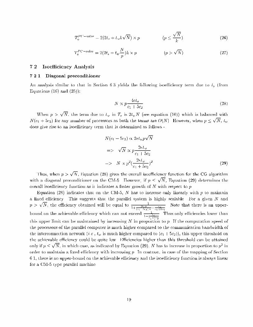
TPC�solveo = 2(2ts + twkpN)� p (p � pNk ) (26)TPC�solveo = 2(2ts + twNp )k � p (p > pN) (27)7.2 Isoe�ciency Analysis7.2.1 Diagonal preconditionerAn analysis similar to that in Section 6.3 yields the following isoe�ciency term due to ts (fromEquations (16) and (25)): N / p 4etsc1 + 5c2 (28)When p > pN , the term due to tw in To is 2twN (see equation (10)) which is balanced withN(c1 + 5c2) for any number of processors as both the terms are O(N). However, when p � pN , twdoes give rise to an isoe�ciency term that is determined as follows -N(c1 + 5c2) / 2etwppN=> pN / p 2etwc1 + 5c2=> N / p2( 2etwc1 + 5c2 )2 (29)Thus, when p > pN , Equation (28) gives the overall isoe�ciency function for the CG algorithmwith a diagonal preconditioner on the CM-5. However, if p � pN , Equation (29) determines theoverall isoe�ciency function as it indicates a faster growth of N with respect to p.Equation (28) indicates that on the CM-5, N has to increase only linearly with p to maintaina �xed e�ciency. This suggests that the parallel system is highly scalable. For a given N andp > pN , the e�ciency obtained will be equal to 11+ 2tsp(c1+5c2)N+ twc1+5c2 . Note that there is an upper-bound on the achievable e�ciency which can not exceed 11+ twc1+5c2 . Thus only e�ciencies lower thanthis upper limit can be maintained by increasing N in proportion to p. If the computation speed ofthe processors of the parallel computer is much higher compared to the communication bandwidth ofthe interconnection network (i.e., tw is much higher compared to (c1 +5c2)), this upper threshold onthe achievable e�ciency could be quite low. E�ciencies higher than this threshold can be attainedonly if p � pN , in which case, as indicated by Equation (29), N has to increase in proportion to p2 inorder to maintain a �xed e�ciency with increasing p. In contrast, in case of the mapping of Section6.1, there is no upper-bound on the achievable e�ciency and the isoe�ciency function is always linearfor a CM-5 type parallel machine.19

?6 ...................................................

.....................................

Vector bMatrix AN

Pp�1----P2P1P0... . .... . . . . . . . ...... .. . . .. . . .. . ...... . ....... .............. .

. . ........ ... . . . . . ..... ......... . . ... ......... .......... ..... ... ...... . . ...... . ...... .. . .. .. .. . ..... ............... ..... .. ... ..... .. ..... . . . .......... .. ......

Figure 7: Partition of a banded sparse matrix and a vector among the processors.7.2.2 IC preconditionerFor this case, W is given by Equation (3). This equation is similar to Equation (16) except that theconstant is di�erent. From the expressions for To for this case, it can be seen that even the terms inTo for the IC preconditioner di�er, if at all, from those in the To for the diagonal preconditioner bya constant factor of (k + 1). Therefore the isoe�ciency functions for the IC preconditioner will besimilar to those for the diagonal preconditioner, but the constants associated with the terms will bedi�erent and will depend on chosen value of k.The upper-bound on the achievable e�ciency on a fully connected network when p > pN is now11+ (k+1)tw�(k) instead of 11+ twc1+5c2 , as in the case of the diagonal preconditioner. The typical values of kvary from 2 to 4. It is observed that for typical values of c1 and c2 for a machine like the CM-5,1c1+5c2 < k+1�(k) for k = 2 and k = 3, and 1c1+5c2 � k+1�(k) for k = 4. As a result, it is possible toobtain higher e�ciencies using a diagonal preconditioner than the IC preconditioner, and in case ofthe IC preconditioner, e�ciencies decrease as k increases. This trend is totally opposite to that forthe data mapping scheme of Section 6.1 in which the IC preconditioner yields better e�ciencies thanthe diagonal preconditioner and the e�ciencies increase with k.8 Scalability analysis: unstructured sparse matricesIn this section, we consider a more general form of sparse matrices. Often, such systems are en-countered where the non-zero elements of matrix A occur only within a band around the principaldiagonal. Even if the non-zero elements are scattered throughout the matrix, it is often possible torestrict them to a band through certain re-ordering techniques [4, 5]. Such a system is shown inFigure 7 in which the non-zero elements of the sparse matrix are randomly distributed within a bandalong the principal diagonal. Let the width of the band of the N � N matrix be given by b, andb = �Ny, and 0 � y � 1. Suitable values of the constants � and y can be selected to represent thekind of systems being solved. If � = 1 and y = 1, we have the case of a totally unstructured sparse20

matrix.The matrix A is stored in the Ellpack-Itpack format [24]. In this storage scheme, the non-zeroelements of the matrix are stored in an N �m array while another N �m integer array stores thecolumn numbers of the matrix elements. It can be shown that co-ordinate and the compressed sparsecolumn storage formats incur much higher communication overheads, thereby leading to unscalableparallel formulations. Two other storage schemes, namely jagged diagonals [24] and compressed sparserows involve communication overheads similar to the Ellpack-Itpack scheme, but the latter is theeasiest to work with when the number of non-zero elements is almost the same in each row of thesparse matrix. The matrix A and the vector b are partitioned among p processors as shown in Figure7. The rows and the columns of the matrix and the elements of the vector are numbered from 0 toN � 1. Processor Pi stores Np i to Np (i+ 1) � 1 rows of matrix A and elements with indices from Np ito Np (i+1)� 1 of vector b. The preconditioner and all the other vectors used in the computation arepartitioned similarly.We will study the application of only the diagonal preconditioner in this case; hence the serialexecution time is given by Equation (2). Often the number of non-zero elements per row of the matrixA is not constant but increases with N . Let m = �Nx, where the constants � and x (0 � x � 1) canbe chosen to describe the kind of systems being solved. A more general expression for W , therefore,would be as follows: W = c1N + c2�N1+x (30)8.1 Communication overheadsFor the diagonal preconditioner, TPC�solveo = 0 as discussed in Section 6. It can be shown thatTMatrix�V ectoro dominates T Inner�Prodo for most practical cases. Therefore, TMatrix�V ectoro can beconsidered to represent the overall overhead To for the case of unstructured sparse matrices.If the distribution of non-zero elements in the matrix is unstructured, each row of the matrix couldcontain elements belonging to any column. Thus, for matrix-vector multiplication, any processor couldneed a vector element that belongs to any other processor. As a result, each processor has to sendits portion of the vector of size Np to every other processor. If the bandwidth of the matrix A is b,then the ith row of the matrix can contain elements belonging to columns i � b2 to i + b2 . Since aprocessor contains Np rows of the matrix and Np elements of each vector, it will need the elements ofthe vector that are distributed among the processors that lie within a distance of bp2N on its eitherside; i.e., processor Pi needs to communicate with all the processors Pj such that i� bp2N � j < i andi < j � i+ bp2N . Thus the total number of communication steps in which each processor can acquireall the data it needs to perform matrix-vector multiplication will be bpN . As a result, the followingexpression gives the value of To for b = �Ny.To = (ts�pNy�1 + tw�Ny)� p (31)It should be noted that this overhead is the same for all architectures under consideration in thispaper from a linear array to a fully connected network.21

8.2 Isoe�ciency analysisThe size W of the problem at hand is given by Equation (30), which may be greater than O(N) forx > 0. Strictly speaking, the isoe�ciency function is de�ned as the rate at which the problem sizeneeds to grow as a function of p to maintain a �xed e�ciency. However, to simplify the interpretationof the results, in this section we will measure the scalability in terms of the rate at which N (the sizeof the linear system of equations to be solved) needs to grow with p rather than rate at which thequantity c1N + c2�N1+x should grow with respect to p.According to Equation (1), the following condition must be satis�ed in order to maintain a �xede�ciency E: c1N + c2�N1+x = E1�E (ts�p2Ny�1 + tw�pNy)=> c2�Nx+y + c1Ny � E1�E tw�pN2y�1 � E1�E ts�p2N2y�2 = 0 (32)=> N = fE(p; x; y; �; �; tw ; ts; c1; c2) (33)From Equation (32), it is not possible to compute the isoe�ciency function fE in a closed formfor general x and y. However, Equation (32) can be solved for N for speci�c values of x and y. We,therefore, compute the isoe�ciency functions for a few interesting cases that result from assigningsome typical values to the parameters x and y. Table 1 gives a summary of the scalability analysisfor these cases. In order to maintain the e�ciency at some �xed value E, the size N of the systemhas to grow according to the expression in the third column of the Table 1, where e = E1�E .The above analysis shows that a PCG iteration is unscalable for a totally unstructured sparsematrix of coe�cients with a constant number of non-zero elements in each row. However, it can berendered scalable by either increasing the number of non-zero elements per row as a function of thematrix size, or by restricting the non-zero elements into a band of width less than O(N) for an N�Nmatrix using some re-ordering scheme. Various techniques for re-ordering sparse systems to yieldbanded or partially banded sparse matrices are available [4, 5]. These techniques may vary in theircomplexity and e�ectiveness. By using Equation (32) the bene�t of a certain degree of re-orderingcan be quantitatively determined in terms of improvement in scalability.In this section we have presented the results for the diagonal preconditioner only. However, the useof the IC preconditioner does not have a signi�cant impact on the overall scalability of the algorithm.If a method similar to the one discussed in Section 6.1 is used, solving the system M z = r forthe preconditioner M will be equivalent to two matrix-vector multiplications, where the band of thematrix is k times wider than that of matrix A if k powers of L and ~LT are computed (see Section6.1). Thus, the expressions for both W and To will be very similar to those in case of the diagonalpreconditioner, except that the constants will be di�erent.9 Experimental results and their interpretationsThe analytical results derived in the earlier sections of the paper were veri�ed through experimen-tal data obtained by implementing the PCG algorithm on the CM-5. Both block-tridiagonal and22

Parameter values Isoe�ciency function Interpretationin terms of scalability1. x = 0, y = 1 Does not exist Unscalable2. x = 0, y = 12 N / p2( e�twc1+c2�)2 O(p2) scalability(moderately scalable)3. x = 1, y = 1 N / p etw�+pe2t2w�2+4c2��ets2c2� Linearly scalable witha high constant4. x = 0, y = 0 N / p etw�2(c1+c2�) �1 +r1 + 4ts(c1+c2�)et2w� � Linear scalability(highly scalable)5. x = 12 , y = 12 N / p etw�2c2� �1 +q1 + 4tsc2�et2w� � Linear scalability(highly scalable)Table 1: Scalability of a PCG iteration with unstructured sparse matrices of coe�cients. The averagenumber of entries in each row of the N � N matrix is �Nx and these entries are located within aband of width �Ny along the principal diagonal.unstructured sparse symmetric positive de�nite matrices were generated randomly and used as testcases. The degree of diagonal dominance of the matrices was controlled such that the algorithmperformed enough number of iterations to ensure the accuracy of our timing results. Often, slightvariation in the number of iterations was observed as di�erent number of processors were used. In theparallel formulation of the PCG algorithm, both matrix-vector multiplication and the inner productcomputation involve communication of certain terms among the processors which are added up toyield a certain quantity. For di�erent values of p, the order in which these terms are added couldbe di�erent. As a result, due to limited precision of the data, the resultant sum may have a slightlydi�erent value for di�erent values of p. Therefore, the criterion for convergence might not be satis�edafter exactly the same number of iterations for all p. In our experiments, we normalized the parallelexecution time with respect to the number of iterations in the serial case in order to compute thespeedups and e�ciencies accurately. Sparse linear systems with matrix dimension varying from 400 toover 64,000 were solved using up to 512 processors. For block-tridiagonal matrices, we implementedthe PCG algorithms using both the diagonal and the IC preconditioners. For unstructured sparsematrices, only the diagonal preconditioner was used. The con�guration of the CM-5 used in ourexperiments had only a SPARC processor on each node which delivered approximately 1 MFLOPS(double-precision) in our implementation. The message startup time for the program was observedto be about 150 microseconds and the per-word transfer time for 8 byte words was observed to be23

050100150200

0 50 100 150 200 250 300 350 400"S

p!

N = 40000 33 3 3

3N = 25600 ++ ++ + + + +N = 10000 22 22 2 2

Figure 8: Speedup curves for block-tridiagonal matrices with diagonal preconditioner.about 3 microseconds3.Figure 8 shows experimental speedup curves for solving problems of di�erent sizes using thediagonal preconditioner on block-tridiagonal matrices. As expected, for a given number of processors,the speedup increases with increasing problem size. Also, for a given problem size, the speedup doesnot continue to increase with the number of processors, but tends to saturate.Recall that the use of the IC preconditioner involves substantially more computation per iterationof the PCG algorithm over a simple diagonal preconditioner, but it also reduces the number ofiterations signi�cantly. As the approximation of the inverse of the preconditioner matrix is made moreaccurate (i.e., k is increased, as discussed in Section 5.2), the computation per iteration continues toincrease, while the number of iterations decreases. The overall performance is governed by the amountof increase in the computation per iteration and the reduction in the number of iterations. As discussedin Section 6.3.2, for the same number of processors, an implementation with the IC preconditionerwill obtain a higher e�ciency4 (and hence speedup) than one with the diagonal preconditioner. Evenin case of the IC preconditioner, speedups will be higher for higher values of k. Figure 9 shows thee�ciency curves for the diagonal preconditioner and the IC preconditioner for k = 2, 3 and 4 for agiven problem size. From this �gure it is clear that one of the IC preconditioning schemes may yield abetter overall execution time in a parallel implementation due to a better speedup than the diagonalpreconditioning scheme, even if the latter is faster in a serial implementation. For instance, assume3These values do not necessarily re ect the communication speed of the hardware but the overheads observed forour implementation. For instance copying the data in and out of the bu�ers in the program contributes to the per-word overhead. Moreover, the machine used in the experiments was still in beta testing phase, hence the performanceobtained in our experiments may not be indicative of the achievable performance of the machine.4The e�ciency of a parallel formulation is computed with respect to an identical algorithm running on a singleprocessor. 24

0.20.30.40.50.60.70.8

0 50 100 150 200 250 300 350 400"E

p!

IC, k = 4 33 3 3 3 3IC, k = 3 ++ + + + +IC, k = 2 22 2 2 2 2Diagonal �� � � � �

Figure 9: E�ciency curves for the diagonal and the IC preconditioner with a 1600 � 1600 matrix ofcoe�cients.that on a serial machine the PCG algorithm runs 1.2 times faster with a diagonal preconditionerthan with the IC preconditioner for a certain system of equations. As shown in Figure 9, with 256processors on the CM-5, the IC preconditioner implementation with k = 3 executes with an e�ciencyof about 0.4 for an 80 � 80 �nite di�erence grid, while the diagonal preconditioner implementationattains an e�ciency of only about 0.26 on the same system. Therefore, unlike on a serial computer,on a 256 processor CM-5 the IC preconditioner implementation for this system with k = 3 will befaster by a factor of 0:40:26 � 1:01:2 � 1:3 than a diagonal preconditioner implementation.In Figure 10, experimental isoe�ciency curves are plotted for the two preconditioners by experi-mentally determining the e�ciencies for di�erent values of N and p and then selecting and plottingthe (N;P ) pairs with nearly the same e�ciencies. As predicted by Equations (17), (18) and (21),the N versus p curves for a �xed e�ciency are straight lines. These equations, as well as Figure 10,suggest that this is a highly scalable parallel system and requires only a linear growth of problem sizewith respect to p to maintain a certain e�ciency. This �gure also shows that the IC preconditionerneeds a smaller problem size than the diagonal preconditioner to achieve the same e�ciency. Forthe same problem size, the IC preconditioner can use more processors at the same e�ciency, therebydelivering higher speedups than the diagonal preconditioner.A comparison of the overhead functions for the data partitioning schemes described in Sections 6and 7 clearly shows that the overhead due to tw is higher in the latter scheme. This extra overheadtranslates into reduced e�ciencies which can be seen from Figure 11. This �gure shows the e�ciencyobtained experimentally on the CM-5 as a function of problem size for the two mapping schemesfor 256 processors. As expected, the block mapping described in Section 6 performs better than thesimple rowwise partitioning described in Section 7.25

0100002000030000400005000060000

0 50 100 150 200 250 300 350 400"N

p!E = 0:8 (diag.) 33 3 3 3E = 0:8 (IC) ++ + + + +

E = 0:7 (diag.) 222 2 2 2 2 2 2E = 0:7 (IC) �� � � � � �

Figure 10: Isoe�ciency curves for the two preconditioning schemes.

00.10.20.30.40.50.60.70.8

0 10000 20000 30000 40000 50000 60000"E

N! Block PartitioningRowwise PartitioningFigure 11: E�ciency curves for the two partitioning schemes on the CM-5 with 256 processors.26

00.10.20.30.40.50.60.70.8

0 10000 20000 30000 40000 50000 60000"E

N!

Block PartitioningRowwise Partitioning

Figure 12: E�ciency curves for the two mapping schemes on a ten times faster CM-5 with 256processors.The di�erence between the e�ciencies obtained for the two schemes will become even more appar-ent if the algorithm is executed on a machine with the same bandwidth of communication channelsbut much faster CPU's. We simulated the e�ect of 10 times faster CPU's by arti�cially loweringthe communication channel bandwidth by a factor of 10 (this was done by sending 10 times biggermessages) and dividing the total execution time by 10. Figure 12 shows the experimental e�ciencycurves for the two schemes for this simulated machine. It can be seen from this �gure that the rowwisepartitioning of Section 7 is a�ected much more seriously than block partitioning described in Section6. Also, as discussed in Section 7.2.1, the e�ciency in case of the rowwise scheme su�ers from asaturation and increasing the problem size beyond a point does not seem to improve the achievede�ciency.Figure 13 shows plots of e�ciency versus problem size for three di�erent values of p for a totallyunstructured sparse matrix with a �xed number of non-zero elements in each row. As discussed inSection 8.2, this kind of a matrix leads to an unscalable parallel formulation of the CG algorithm.This fact is clearly re ected in Figure 13. Not only does the e�ciency drop rapidly as the number ofprocessors are increased, but also an increase in problem size does not su�ce to counter this drop ine�ciency. For instance, using 40 processors, it does not seem possible to attain the e�ciency of 16processors, no matter how big a problem is being solved.Figures 14 and 15 show how the parallel CG algorithm for unstructured sparse matrices can bemade scalable by either con�ning the non-zero elements within a band of width < O(N), or byincreasing the number of non-zero elements in each row as a function of N . Figure 14 shows theexperimental isoe�ciency curves for a banded unstructured sparse matrix with a bandwidth of 2pNand 6 non-zero elements per row. The curves were drawn by picking up (N; p) pairs that yielded27

00.10.20.30.40.50.6

0 2000 4000 6000 8000 10000 12000 14000"E

N!

p = 8 33 3 3 3p = 16 ++ + + +p = 40 22 2 2 2

Figure 13: E�ciency plots for unstructured sparse matrices with �xed number of non-zero elementsper row.

010000200003000040000500000 10000 20000 30000 40000 50000 60000 70000

"Np2! E = 0:8 33 3 3 3

3E = 0:7 ++ + +

+ +

Figure 14: Isoe�ciency curves for banded unstructured sparse matrices with �xed number of non-zeroelements per row. 28

050001000015000200002500030000350004000045000

10 20 30 40 50 60 70"N

p! E = 0:25 33 3 3 3 3

Figure 15: An isoe�ciency curve for unstructured sparse matrices with the number of non-zero ele-ments per row increasing with the matrix size.nearly the same e�ciency on the CM-5 implementation, and then plotting N with respect to p2. Asshown in Table 1, the isoe�ciency function is O(p2) and a linear relation between N and p2 in Figure14 con�rms this. Figure 15 shows the isoe�ciency curve for E = 0:25 for a totally unstructuredN�Nsparse matrix with 0:0015N non-zero elements in each row. As shown in Table 1, the isoe�ciencyfunction is linear in this case, although the constant associated with it is quite large because of theterms 2c2� in the denominator, � being 0.0015.10 Summary of results and concluding remarksIn this paper we have studied the performance and scalability of an iteration of the PreconditionedConjugate Gradient algorithm on a variety of parallel architectures.It is shown that block-tridiagonal matrices resulting from the discretization of a 2-dimensionalself-adjoint elliptic partial di�erential equation via �nite di�erences lead to highly scalable parallelformulations of the CG method on a parallel machine like the CM-5 with an appropriate mapping ofdata onto the processors. On this architecture, speedups proportional to the number of processorscan be achieved by increasing the problem size almost linearly with the number of processors. Thereason is that on the CM-5, the control network practically eliminates the communication overhead incomputing inner-products of vectors, whereas on more conventional parallel machines with signi�cantmessage startup times, it turns out to be the costliest operation in terms of overheads and a�ectsthe overall scalability. The isoe�ciency function for a PCG iteration with a block-tridiagonal matrixis O(p) on the CM-5, O(p log p) on a hypercube, and O(ppp) on a mesh. In terms of scalability,if the number of processors is increased from 100 to 1000, the problem size will have to increased29

32 times on a mesh, 15 times on a hypercube, and only 10 times on the CM-5 to obtain ten timeshigher speedups. Also, the e�ect of message startup time ts on the speedup is much more signi�canton a typical hypercube or a mesh than on the CM-5. However, for some iterative algorithms likethe Jacobi method, linear scalability can be obtained even on these architectures by performing theconvergence check at a suitably reduced frequency.The current processors used on the CM-5 are SPARC processors that deliver about 1 MFLOPS(double-precision) each in our implementation. These processors are soon expected to be augmentedwith vector units that may increase the net performance by a factor of 10 to 30. This will reducethe ratio of communication speed to computation speed by a factor a 10 to 30. The message startuptime using the current unoptimized communication routines is about 150 microseconds. A 5 to 10times reduction in ts in the near future is quite conceivable due to software improvement. After theseimprovements, the CM-5 will be a massively parallel machine with hardware parameters close to thoseof the hypothetical machine described in Section 6.4. For these values of the machine parameters,a high inter-processor communication bandwidth will be crucial for obtaining good e�ciencies. Thereason is that although the isoe�ciency function of an iteration of the PCG algorithm is linear withrespect to p, it is also proportional to the square of E1�E tw. Moreover, at such high processor speeds,the simple mapping scheme described in Section 7 will be highly impractical.We have shown that in case of the block-tridiagonal matrices, the truncated Incomplete Choleskypreconditioner can achieve higher e�ciencies than a simple diagonal preconditioner if the data map-ping scheme of Section 6.1 is used. The use of the IC preconditioner usually signi�cantly cuts downthe number of iterations required for convergence. However, it involves solving a linear system ofequations of the formM z = r in each iteration. This is a computationally costly operation and mayo�set the advantage gained by fewer iterations. Even if this is the case for the serial algorithm, ina parallel implementation the IC preconditioner may outperform the diagonal preconditioner as thenumber of processors are increased. This is because a parallel implementation with IC preconditionerexecutes at a higher e�ciency than one with a diagonal preconditioner.If the matrix of coe�cients of the linear system of equations to be solved is an unstructuredsparse matrix with a constant number of non-zero elements in each row, a parallel formulation of thePCG method will be unscalable on any practical massage passing architecture unless some orderingis applied to the sparse matrix. The e�ciency of parallel PCG with an unordered sparse matrix willalways drop as the number of processors is increased and no increase in the problem size is su�cientto counter this drop in e�ciency. The system can be rendered scalable if either the non-zero elementsof the N � N matrix of coe�cients can be con�ned in a band whose width is less than O(N), orthe number of non-zero elements per row increases with N , where N is the number of simultaneousequations to be solved. The scalability increases as the number of non-zero elements per row inthe matrix of coe�cients is increased and/or the width of the band containing these elements isreduced.5 Both the number of non-zero elements per row and the width of the band containing theseelements depend on the characteristics of the system of equations to be solved. In particular, thenon-zero elements can be organized within a band by using some re-ordering techniques [4, 5]. Such5Unstructured sparse matrices arise in several applications. More details on scalable parallel formulations of sparsematrix-vector multiplication (and hence, iterative methods such as PCG) involving unstructured matrices arising in�nite element problems are discussed in [18]. 30

restructuring techniques can improve the e�ciency (for a given number of processors, problem size,machine architecture, etc.) as well as the asymptotic scalability of the PCG algorithm.References[1] Edward Anderson. Parallel implementation of preconditioned conjugate gradient methods for solving sparse systemsof linear equations. Technical Report 805, Center for Supercomputing Research and Development, University ofIllinois, Urbana, IL, 1988.[2] Cevdet Aykanat, Fusun Ozguner, Fikret Ercal, and Ponnuswamy Sadayappan. Iterative algorithms for solution oflarge sparse systems of linear equations on hypercubes. IEEE Transactions on Computers, 37(12):1554{1567, 1988.[3] D. L. Eager, J. Zahorjan, and E. D. Lazowska. Speedup versus e�ciency in parallel systems. IEEE Transactionson Computers, 38(3):408{423, 1989.[4] A. George and J. W.-H. Liu. Computer Solution of Large Sparse Positive De�nite Systems. Prentice-Hall, Engle-wood Cli�s, NJ, 1981.[5] N. E. Gibbs, W. G. Poole, and P. K. Stockmeyer. A comparison of several bandwidth and pro�le reductionalgorithms. ACM Transactions on Mathematical Software, 2:322{330, 1976.[6] Gene H. Golub and Charles Van Loan. Matrix Computations: Second Edition. The Johns Hopkins UniversityPress, Baltimore, MD, 1989.[7] Ananth Grama, Anshul Gupta, and Vipin Kumar. Isoe�ciency: Measuring the scalability of parallel algorithmsand architectures. IEEE Parallel and Distributed Technology, 1(3):12{21, August, 1993. Also available as TechnicalReport TR 93-24, Department of Computer Science, University of Minnesota, Minneapolis, MN.[8] Anshul Gupta and Vipin Kumar. A scalable parallel algorithm for sparse matrix factorization. Technical Report94-19, Department of Computer Science, University of Minnesota, Minneapolis, MN, 1994. A short version appearsin Supercomputing '94 Proceedings. TR available in users/kumar at anonymous FTP site ftp.cs.umn.edu.[9] Anshul Gupta and Vipin Kumar. The scalability of FFT on parallel computers. IEEE Transactions on Paralleland Distributed Systems, 4(8):922{932, August 1993. A detailed version available as Technical Report TR 90-53,Department of Computer Science, University of Minnesota, Minneapolis, MN.[10] John L. Gustafson. Reevaluating Amdahl's law. Communications of the ACM, 31(5):532{533, 1988.[11] John L. Gustafson, Gary R. Montry, and Robert E. Benner. Development of parallel methods for a 1024-processorhypercube. SIAM Journal on Scienti�c and Statistical Computing, 9(4):609{638, 1988.[12] S. W. Hammond and Robert Schreiber. E�cient ICCG on a shared-memory multiprocessor. International Journalof High Speed Computing, 4(1):1{22, March 1992.[13] Kai Hwang. Advanced Computer Architecture: Parallelism, Scalability, Programmability. McGraw-Hill, New York,NY, 1993.[14] C. Kamath and A. H. Sameh. The preconditioned conjugate gradient algorithm on a multiprocessor. In R. Vichn-evetsky and R. S. Stepleman, editors, Advances in Computer Methods for Partial Di�erential Equations. IMACS,1984.[15] Alan H. Karp and Horace P. Flatt. Measuring parallel processor performance. Communications of the ACM,33(5):539{543, 1990.[16] S. K. Kim and A. T. Chronopoulos. A class of Lanczos-like algorithms implemented on parallel computers. ParallelComputing, 17:763{777, 1991.[17] Kouichi Kimura and Ichiyoshi Nobuyuki. Probabilistic analysis of the e�ciency of the dynamic load distribution.In The Sixth Distributed Memory Computing Conference Proceedings, 1991.[18] Vipin Kumar, Ananth Grama, Anshul Gupta, and George Karypis. Introduction to Parallel Computing: Designand Analysis of Algorithms. Benjamin/Cummings, Redwood City, CA, 1994.31

[19] Vipin Kumar and Anshul Gupta. Analyzing scalability of parallel algorithms and architectures. Technical ReportTR 91-18, Department of Computer Science Department, University of Minnesota, Minneapolis, MN, 1991. Toappear in Journal of Parallel and Distributed Computing, 1994. A shorter version appears in Proceedings of the1991 International Conference on Supercomputing, pages 396-405, 1991.[20] C. E. Leiserson. Fat-trees: Universal networks for hardware e�cient supercomputing. In Proceedings of the 1985International Conference on Parallel Processing, pages 393{402, 1985.[21] Rami Melhem. Toward e�cient implementation of preconditioned conjugate gradient methods on vector super-computers. International Journal of Supercomputer Applications, I(1):70{97, 1987.[22] Daniel Nussbaum and Anant Agarwal. Scalability of parallel machines. Communications of the ACM, 34(3):57{61,1991.[23] S. Ranka and S. Sahni. Hypercube Algorithms for Image Processing and Pattern Recognition. Springer-Verlag, NewYork, NY, 1990.[24] Youcef Saad. SPARSKIT: A basic tool kit for sparse matrix computations. Technical Report 90-20, ResearchInstitute for Advanced Computer Science, NASA Ames Research Center, Mo�et Field, CA, 1990.[25] Youcef Saad and M. H. Schultz. Parallel implementations of preconditioned conjugate gradient methods. TechnicalReport YALEU/DCS/RR-425, Yale University, Department of Computer Science, New Haven, CT, 1985.[26] Vineet Singh, Vipin Kumar, Gul Agha, and Chris Tomlinson. Scalability of parallel sorting on mesh multicomputers.International Journal of Parallel Programming, 20(2), 1991.[27] Zhimin Tang and Guo-Jie Li. Optimal granularity of grid iteration problems. In Proceedings of the 1990 Interna-tional Conference on Parallel Processing, pages I111{I118, 1990.[28] Fredric A. Van-Catledge. Towards a general model for evaluating the relative performance of computer systems.International Journal of Supercomputer Applications, 3(2):100{108, 1989.[29] Henk A. van der Vorst. A vectorizable variant of some ICCG methods. SIAM Journal on Scienti�c and StatisticalComputing, III(3):350{356, 1982.[30] Henk A. van der Vorst. Large tridiagonal and block tridiagonal linear systems on vector and parallel computers.Parallel Computing, 5:45{54, 1987.[31] Jinwoon Woo and Sartaj Sahni. Computing biconnected components on a hypercube. Journal of Supercomputing,June 1991. Also available as Technical Report TR 89-7 from the Department of Computer Science, University ofMinnesota, Minneapolis, MN.[32] Patrick H. Worley. The e�ect of time constraints on scaled speedup. SIAM Journal on Scienti�c and StatisticalComputing, 11(5):838{858, 1990.[33] J. R. Zorbas, D. J. Reble, and R. E. VanKooten. Measuring the scalability of parallel computer systems. InSupercomputing '89 Proceedings, pages 832{841, 1989.

32