arX

iv:1

706.

0517

1v1

[cs

.AI]

16

Jun

2017

Improving Scalability of Inductive Logic Programming

via Pruning and Best-Effort Optimisation

Mishal Kazmi1, Peter Schüller2,C , and Yücel Saygın1

1 Faculty of Engineering and Natural Science,Sabanci University,Istanbul, Turkey

{mishalkazmi,ysaygin}@sabanciuniv.edu2 Faculty of Engineering,

Marmara University,Istanbul, Turkey

peter.schuller@marmara.edu.tr / schueller.p@gmail.com

Technical Report: manuscript accepted for publication at Expert Systems With Applications (Elsevier).

c© 2017. This manuscript version is made available under the CC-BY-NC-ND 4.0 license.

http://creativecommons.org/licenses/by-nc-nd/4.0/ .

Abstract

Inductive Logic Programming (ILP) combines rule-based and statistical artificial intelligencemethods, by learning a hypothesis comprising a set of rules given background knowledge and con-straints for the search space. We focus on extending the XHAIL algorithm for ILP which is basedon Answer Set Programming and we evaluate our extensions using the Natural Language Processingapplication of sentence chunking. With respect to processing natural language, ILP can cater for theconstant change in how we use language on a daily basis. At the same time, ILP does not requirehuge amounts of training examples such as other statistical methods and produces interpretable re-sults, that means a set of rules, which can be analysed and tweaked if necessary. As contributions weextend XHAIL with (i) a pruning mechanism within the hypothesis generalisation algorithm whichenables learning from larger datasets, (ii) a better usage of modern solver technology using recentlydeveloped optimisation methods, and (iii) a time budget that permits the usage of suboptimal results.We evaluate these improvements on the task of sentence chunking using three datasets from a recentSemEval competition. Results show that our improvements allow for learning on bigger datasetswith results that are of similar quality to state-of-the-art systems on the same task. Moreover, wecompare the hypotheses obtained on datasets to gain insights on the structure of each dataset.

1 Introduction

Inductive Logic Programming (ILP) (Muggleton and De Raedt, 1994) is a formalism where a set of logi-cal rules is learned from a set of examples and a background knowledge theory. By combining rule-basedand statistical artificial intelligence, ILP overcomes the brittleness of pure logic-based approaches and thelack of interpretability of models of most statistical methods such as neural networks or support vectormachines. We here focus on ILP that is based on Answer Set Programming (ASP) as our underlyinglogic programming language because we aim to apply ILP to Natural Language Processing (NLP) ap-plications such as Machine Translation, Summarization, Coreference Resolution, or Parsing that requirenonmonotonic reasoning with exceptions and complex background theories.

In our work, we apply ILP to the NLP task of sentence chunking. Chunking, also known as ‘shal-low parsing’, is the identification of short phrases such as noun phrases which mainly rely on Part ofSpeech (POS) tags. In our experiments on sentence chunking (Tjong Kim Sang and Buchholz, 2000) weencountered several problems with state-of-the-art ASP-based ILP systems XHAIL (Ray, 2009), ILED

1

(Katzouris et al., 2015), and ILASP2 (Law et al., 2015). XHAIL and ILASP2 showed scalability issuesalready with 100 sentences as training data. ILED is designed to be highly scalable but failed in thepresence of simple inconsistencies in examples. We decided to investigate the issue in the XHAIL system,which is open-source and documented well, and we made the following observations:

(i) XHAIL only terminates if it finds a provably optimal hypothesis,

(ii) the hypothesis search is done over all potentially beneficial rules that are supported by at least oneexample, and

(iii) XHAIL contains redundancies in hypothesis search and uses outdated ASP technology.

In larger datasets, observation (i) is unrealistic, because finding a near-optimal solution is much easierthan proving optimality of the best solution, moreover in classical machine learning suboptimal solutionsobtained via non-exact methods routinely provide state-of-the-art results. Similarly, observation (ii)makes it harder to find a hypothesis, and it generates an overfitting hypotheses which contains rules thatare only required for a single example. Observation (iii) points out an engineering problem that can beremedied with little theoretical effort.

To overcome the above issues, we modified the XHAIL algorithm and software, and we performedexperiments on a simple NLP chunking task to evaluate our modifications.

In detail, we make the following contributions.

• We extend XHAIL with best-effort optimisation using the newest ASP optimisation technol-ogy of unsat-core optimisation (Andres et al., 2012) with stratification (Alviano et al., 2015b;Ansótegui et al., 2013) and core shrinking (Alviano and Dodaro, 2016) using the WASP2 (Alviano et al.,2013, 2015a) solver and the Gringo (Gebser et al., 2011) grounder. We also extend XHAIL to pro-vide information about the optimality of the hypothesis.

• We extend the XHAIL algorithm with a parameter Pr for pruning, such that XHAIL searches forhypotheses without considering rules that are supported by fewer than Pr examples.

• We eliminate several redundancies in XHAIL by changing its internal data structures.

• We describe a framework for chunking with ILP, based on preprocessing with Stanford Core NLP(Manning et al., 2014) tools.

• We experimentally analyse the relationship between the pruning parameter, number of trainingexamples, and prediction score on the sentence chunking (Tjong Kim Sang and Buchholz, 2000)subtask of iSTS at SemEval 2016 (Agirre et al., 2016).

• We discuss the best hypothesis found for each of the three datasets in the SemEval task, and wediscuss what can be learned about the dataset from these hypotheses.

Only if we use all the above modifications together, XHAIL becomes applicable in this chunking task.By learning a hypothesis from 500 examples, we can achieve results competitive with state-of-the-artsystems used in the SemEval 2016 competition.

Our extensions and modifications of the XHAIL software are available in a public fork of the officialXHAIL Git repository (Bragaglia and Schüller, 2016).

In Section 2 we provide an overview of logic programming and ILP. Section 3 gives an account ofrelated work and available ILP tools. In Section 4 we describe the XHAIL system and our extensions ofpruning, best-effort optimisation, and further improvements. Section 5 gives details of our representationof the chunking task. In Section 6 we discuss empirical experiments and results. We conclude in Section7 with a brief outlook on future work.

2 Background

We next introduce logic programming and based on that inductive logic programming.

2

2.1 Logic Programming

A logic programs theory normally comprises of an alphabet (variable, constant, quantifier, etc), vocab-ulary, logical symbols, a set of axioms and inference rules (Lloyd, 2012). A logic programming systemconsists of two portions: the logic and control. Logic describes what kind of problem needs to be solvedand control is how that problem can be solved. An ideal of logic programming is for it to be purelydeclarative. The popular Prolog (Clocksin and Mellish, 2003) system evaluates rules using resolution,which makes the result of a Prolog program depending on the order of its rules and on the order ofthe bodies of its rules. Answer Set Programming (ASP) (Brewka et al., 2011; Gebser et al., 2012a) is amore recent logic programming formalism, featuring more declarativity than Prolog by defining seman-tics based on Herbrand models (Gelfond and Lifschitz, 1988). Hence the order of rules and the orderof the body of the rules does not matter in ASP. Most ASP programs follow the Generate-Define-Teststructure (Lifschitz, 2002) to (i) generate a space of potential solutions, (ii) define auxiliary concepts,and (iii) test to invalidate solutions using constraints or incurring a cost on non-preferred solutions.

An ASP program consists of rules of the following structure:

a← b1, . . . , bm,not bm+1, . . . ,not bn

where a, bi are atoms from a first-order language, a is the head and b1, . . . ,not bn is the body of the rule,and not is negation as failure. Variables start with capital letters, facts (rules without body condition)are written as ‘a.’ instead of ‘a← ’. Intuitively a is true if all positive body atoms are true and nonegative body atom is true.

The formalism can be understood more clearly by considering the following sentence as a simpleexample:

Computers are normally fast machines unless they are old.

This would be represented as a logical rule as follows:

fastmachine(X)← computer(X),not old(X).

where X is a variable, fastmachine , computer , and old are predicates, and old(X ) is a negated atom.Adding more knowledge results in a change of a previous understanding, this is common in human

reasoning. Classical First Order Logic does not allow such non-monotonic reasoning, however, ASP wasdesigned as a commonsense reasoning formalism: a program has zero or more answer sets as solutions,adding knowledge to the program can remove answer sets as well as produce new ones. Note that ASPsemantics rule out self-founded truths in answer sets. We use the ASP formalism due to its flexibilityand declarativity. For formal details and a complete description of syntax and semantics see the ASP-Core-2 standard (Calimeri et al., 2012). ASP has been applied to several problems related to NaturalLanguage Processing, see for example (Mitra and Baral, 2016; Schüller, 2013, 2014, 2016; Schwitter,2012; Sharma et al., 2015). An overview of applications of ASP in general can be found in (Erdem et al.,2016).

2.2 Inductive Logic Programming

Processing natural language based on hand-crafted rules is impractical because human language is con-stantly evolving, partially due to the human creativity of language use. An example of this was recentlynoticed on UK highways where they advised drivers, ‘Don’t Pokémon Go and drive’. Pokémon Go is beinginformally used here as a verb even though it was only introduced as a game a few weeks before the signwas put up. To produce robust systems, it is necessary to use statistical models of language. These modelsare often pure Machine Learning (ML) estimators without any rule components (Manning and Schütze,1999). ML methods work very well in practice, however, they usually do not provide a way for explainingwhy a certain prediction was made, because they represent the learned knowledge in big matrices of realnumbers. Some popular classifiers used for processing natural language include Naive Bayes, DecisionTrees, Neural Networks, and Support Vector Machines (SVMs) (Dumais et al., 1998).

In this work, we focus on an approach that combines rule-based methods and statistics and pro-vides interpretable learned models: Inductive Logic Programming (ILP). ILP is differentiated from MLtechniques by its use of an expressive representation language and its ability to make use of logically

3

encoded background knowledge (Muggleton and De Raedt, 1994). An important advantage of ILP overML techniques such as neural networks is, that a hypothesis can be made readable by translating itinto piece of English text. Furthermore, if annotated corpora of sufficient size are not available or tooexpensive to produce, deep learning or other data intense techniques are not applicable. However, wecan still learn successfully with ILP.

Formally, ILP takes as input a set of examples E, a set B of background knowledge rules, and a setof mode declarations M , also called mode bias. As output, ILP aims to produce a set of rules H calledhypothesis which entails E with respect to B. The search for H with respect to E and B is restrictedby M , which defines a language that limits the shape of rules in the hypothesis candidates and thereforethe complexity of potential hypotheses.

Example 1. Consider the following example ILP instance (M,E,B) (Ray, 2009).

M =

#modeh flies(+bird).#modeb penguin(+bird).#modeb not penguin(+bird).

(1)

E =

#example flies(a).#example flies(b).#example flies(c).#example notflies(d).

(2)

B =

bird(X) :- penguin(X).bird(a).bird(b).bird(c).penguin(d).

(3)

Based on this, an ILP system would ideally find the following hypothesis.

H ={

flies(X) :- bird(X), not penguin(X).}

(4)

3 Related Work

Inductive Logic Programming (ILP) is a rather multidisciplinary field which extends to domains suchas computer science, artificial intelligence, and bioinformatics. Research done in ILP has been greatlyimpacted by Machine Learning (ML), Artificial Intelligence (AI) and relational databases. Quite a fewsurveys (Gulwani et al., 2015; Kitzelmann, 2009; Muggleton et al., 2012) mention about the systems andapplications of ILP in interdisciplinary areas. We next give related work of ILP in general and then focuson ILP applied in the field of Natural Language Processing (NLP).

The foundations of ILP can be found in research by Plotkin (Plotkin, 1970, 1971), Shapiro (Shapiro,1983) and Sammut and Banerji (Sammut and Banerji, 1986). The founding paper of Muggleton (Muggleton,1991) led to the launch of the first international workshop on ILP. The strength of ILP lay in its ability todraw on and extend the existing successful paradigms of ML and Logic Programming. At the beginning,ILP was associated with the introduction of foundational theoretical concepts which included InverseResolution (Muggleton, 1995; Muggleton and Buntine, 1992) and Predicate Invention (Muggleton, 1991;Muggleton and Buntine, 1992). A number of ILP systems were developed along with learning aboutthe theoretical concepts of ILP such as FOIL (Quinlan, 1990) and Golem (Muggleton et al., 1990). Thewidely-used ILP system Progol (Muggleton, 1995) introduced a new logically-based approach to re-finement graph search of the hypothesis space based on inverting the entailment relation. Meanwhile,the TILDE system (De Raedt, 1997) demonstrated the efficiency which could be gained by upgradingdecision-tree learning algorithms to first-order logic, this was soon extended towards other ML problems.Some limitations of Prolog-based ILP include requiring extensional background and negative examples,lack of predicate invention, search limitations and inability to handle cuts. Integrating bottom-up andtop-down searches, incorporating predicate invention, eliminating the need for explicit negative examplesand allowing restricted use of cuts helps in solving these issues (Mooney, 1996).

4

Probabilistic ILP (PILP) also gained popularity (Cussens, 2001a; De Raedt and Kersting, 2008;Muggleton et al., 1996), its Prolog-based systems such as PRISM (Sato et al., 2005) and FAM (Cussens,2001b) separate the actual learning of the logic program from the probabilistic parameters estimationof the individual clauses. However in practice, learning the structure and parameters of probabilisticlogic representation simultaneously has proven to be a challenge (Muggleton, 2002). PILP is mainly aunification of the probabilistic reasoning of Machine Learning with the relational logical representationsoffered by ILP.

Meta-interpretive learning (MIL) (Muggleton et al., 2014) is a recent ILP method which learns re-cursive definitions using Prolog and ASP-based declarative representations. MIL is an extension of theProlog meta-interpreter; it derives a proof by repeatedly fetching the first-order Prolog clauses and ad-ditionally fetching higher-order meta-rules whose heads unify with a given goal, and saves the resultingmeta-substitutions to form a program.

Most ILP research has been aimed at Horn programs which exclude Negation as Failure (NAF).Negation is a key feature of logic programming and provides a means for monotonic commonsensereasoning under incomplete information. This fails to exploit the full potential of normal programs thatallow NAF.

We next give an overview of ILP systems based on ASP that are designed to operate in the presenceof negation. Then we give an overview of ILP literature related to NLP.

3.1 ASP-based ILP Systems

The eXtended Hybrid Abductive Inductive Learning system (XHAIL) is an ILP approach based on ASPthat generalises techniques of language and search bias from Horn clauses to normal logic programs withfull usage of NAF (Ray, 2009). Like its predecessor system Hybrid Abductive Inductive Learning (HAIL)which operated on Horn clauses, XHAIL is based on Abductive Logic Programming (ALP) (Kakas et al.,1992), we give more details on XHAIL in Section 4.

The Incremental Learning of Event Definitions (ILED) algorithm (Katzouris et al., 2015) relies onAbductive-Inductive learning and comprises of a scalable clause refinement methodology based on acompressive summarization of clause coverage in a stream of examples. Previous ILP learners were batchlearners and required all training data to be in place prior to the initiation of the learning process. ILEDlearns incrementally by processing training instances when they become available and altering previousinferred knowledge to fit new observation, this is also known as theory revision. It exploits previouscomputations to speed-up the learning since revising the hypothesis is considered more efficient thanlearning from scratch. ILED attempts to cover a maximum of examples by re-iterating over previouslyseen examples when the hypothesis has been refined. While XHAIL can ensure optimal example coverageeasily by processing all examples at once, ILED does not preserve this property due to a non-global viewon examples.

When considering ASP-based ILP, negation in the body of rules is not the only interesting additionto the overall concept of ILP. An ASP program can have several independent solutions, called answersets, of the program. Even the background knowledge B can admit several answer sets without anyaddition of facts from examples. Therefore, a hypothesis H can cover some examples in one answer set,while others are covered by another answer set. XHAIL and ILED approaches are based on finding ahypothesis that is covering all examples in a single answer set.

The Inductive Learning of Answer Set Programs approach (ILASP) is an extension of the notionof learning from answer sets (Law et al., 2014). Importantly, it covers positive examples bravely (i.e.,in at least one answer set) and ensures that the negation of negative examples is cautiously entailed(i.e., no negative example is covered in any answer set). Negative examples are needed to learn AnswerSet Programs with non-determinism otherwise there is no concept of what should not be in an AnswerSet. ILASP conducts a search in multiple stages for brave and cautious entailment and processes allexamples at once. ILASP performs a less informed hypothesis search than XHAIL or ILED, that meanslarge hypothesis spaces are infeasible for ILASP while they are not problematic for XHAIL and ILED,on the other hand, ILASP supports aggregates and constraints while the older systems do not supportthese. ILASP2 (Law et al., 2015) extends the hypothesis space of ILASP with choice rules and weakconstraints. This permits searching for hypotheses that encode preference relations.

5

3.2 ILP and NLP

From NLP point of view, the hope of ILP is to be able to steer a mid-course between these two alternativesof large-scale but shallow levels of analysis and small scale but deep and precise analysis. ILP shouldproduce a better ratio between breadth of coverage and depth of analysis (Muggleton, 1999). ILP hasbeen applied to the field of NLP successfully; it has not only been shown to have higher accuraciesthan various other ML approaches in learning the past tense of English but also shown to be capable oflearning accurate grammars which translate sentences into deductive database queries (Law et al., 2014).

Except for one early application (Wirth, 1989) no application of ILP methods surfaced until the systemCHILL (Mooney, 1996) was developed which learned a shift-reduce parser in Prolog from a trainingcorpus of sentences paired with the desired parses by learning control rules and uses ILP to learn controlstrategies within this framework. This work also raised several issues regarding the capabilities andtesting of ILP systems. CHILL was also used for parsing database queries to automate the constructionof a natural language interface (Zelle and Mooney, 1996) and helped in demonstrating its ability to learnsemantic mappings as well.

An extension of CHILL, CHILLIN (Zelle et al., 1994) was used along with an extension of FOIL,mFOIL (Tang and Mooney, 2001) for semantic parsing. Where CHILLIN combines top-down andbottom-up induction methods and mFOIL is a top-down ILP algorithm designed keeping imperfectdata in mind, which portrays whether a clause refinement is significant for the overall performance withthe help of a pre-pruning algorithm. This emphasised on how the combination of multiple clause con-structors helps improve the overall learning; which is a rather similar concept to Ensemble Methods instandard ML. Note that CHILLIN pruning is based on probability estimates and has the purpose of deal-ing with inconsistency in the data. Opposed to that, XHAIL already supports learning from inconsistentdata, and the pruning we discuss in Section 4.1 aims to increase scalability.

Previous work ILP systems such as TILDE and Aleph (Srinivasan, 2001) have been applied to pref-erence learning which addressed learning ratings such as good, poor and bad. ASP expresses preferencesthrough weak constraints and may also contain weak constraints or optimisation statements which imposean ordering on the answer sets (Law et al., 2015).

The system of Mitra and Baral (Mitra and Baral, 2016) uses ASP as primary knowledge representa-tion and reasoning language to address the task of Question Answering. They use a rule layer that ispartially learned with XHAIL to connect results from an Abstract Meaning Representation parser andan Event Calculus theory as background knowledge.

4 Extending XHAIL algorithm and system

Initially, we intended to use the latest ILP systems (ILASP2 or ILED) in our work. However, preliminaryexperiments with ILASP2 showed a lack in scalability (memory usage) even for only 100 sentences due tothe unguided hypothesis search space. Moreover, experiments with ILED uncovered several problematiccorner cases in the ILED algorithm that led to empty hypotheses when processing examples that weremutually inconsistent (which cannot be avoided in real-life NLP data). While trying to fix these problemsin the algorithm, further issues in the ILED implementation came up. After consulting the authors of(Mitra and Baral, 2016) we learned that they had the same issues and used XHAIL, therefore we alsoopted to base our research on XHAIL due to it being the most robust tool for our task in comparison tothe others.

Although XHAIL is applicable, we discovered several drawbacks and improved the approach and theXHAIL system. We provide an overview of the parts we changed and then present our modifications.Figure 1 shows in the middle the original XHAIL components and on the right our extension.

XHAIL finds a hypothesis using several steps. Initially the examples E plus background knowledgeB are transformed into a theory of Abductive Logic Programming (Kakas et al., 1992). The Abductionpart of XHAIL explains observations with respect to a prior theory, which yields the Kernel Set, ∆. ∆is a set of potential heads of rules given by M such that a maximum of examples E is satisfied togetherwith B.

Example 2 (continued). Given (M,E,B) from Example 1, XHAIL uses B, E, and the head part of M ,

6

Abduction

Examples E

Background Knowledge B

Mode Bias M (Head)

DeductionMode Bias M (Body)

Generalisation

Induction

Hypothesis

Generalisation(counting)

Pruning

∆ (Kernet Set)

ground K program

non-ground K’ program

ground K program

non-ground K’ program with support counts

subset of K’

ReplacedModified

Figure 1: XHAIL architecture. The dotted line shows the replaced module with our version representedby the thick solid line.

to generate the Kernel Set ∆ by abduction.

∆ =

flies(a)flies(b)flies(c)

The Deduction part uses ∆ and the body part of the mode bias M to generate a ground program K.K contains rules which define atoms in ∆ as true based on B and E.

The Generalisation part replaces constant terms in K with variables according to the mode bias M ,which yields a non-ground program K ′.

Example 3 (continued). From the above ∆ and M from (1), deduction and generalisation yield thefollowing K and K ′.

K =

flies(a) :- bird(a), not penguin(a)flies(b) :- bird(b), not penguin(b)flies(c) :- bird(c), not penguin(c)

K ′ =

flies(X) :- bird(X), not penguin(X)flies(Y) :- bird(Y), not penguin(Y)flies(Z) :- bird(Z), not penguin(Z)

The Induction part searches for the smallest part of K ′ that entails as many examples of E as possiblegiven B. This part of K ′ which can contain a subset of the rules of K ′ and for each rule a subset of bodyatoms is called a hypothesis H .

Example 4 (continued). The smallest hypothesis that covers all examples E in (2) is (4).

We next describe our modifications of XHAIL.

4.1 Kernel Pruning according to Support

The computationally most expensive part of the search in XHAIL is Induction. Each non-ground rulein K ′ is rewritten into a combination of several guesses, one guess for the rule and one additional guessfor each body atom in the rule.

We moreover observed that some non-ground rules in K ′ are generalisations of many different groundrules in K, while some non-ground rules correspond with only a single instance in K. In the following,we say that the support of r in K is the number of ground rules in K that are transformed into r∈K ′

in the Generalisation module of XHAIL (see Figure 1).

7

Intuitively, the higher the support, the more examples can be covered with that rule, and the morelikely that rule or a part of it will be included in the optimal hypothesis.

Therefore we modified the XHAIL algorithm as follows.

• During Generalisation, we keep track of the support of each rule r∈K ′ by counting how often ageneralisation yields the same rule r.

• We add an integer pruning parameter Pr to the algorithm and use only those rules from K ′ in theInduction component that have a support higher than Pr.

This modification is depicted as bold components which replace the dotted Generalisation module inFigure 1.

Pruning has several consequences. From a theoretical point of view, the algorithm becomes incompletefor Pr > 0, because Induction searches in a subset of the relevant hypotheses. Hence Induction might notbe able to find a hypothesis that covers all examples, although such a hypothesis might exist with Pr=0.From a practical point of view, pruning realises something akin to regularisation in classical ML; onlystrong patterns in the data will find their way into Induction and have the possibility to be representedin the hypothesis. A bit of pruning will therefore automatically prevent overfitting and generate moregeneral hypotheses. As we will show in Experiments in Section 6, the pruning allows to configure atrade-off between considering low-support rules instead of omitting them entirely, as well as, finding amore optimal hypothesis in comparison to a highly suboptimal one.

4.2 Unsat-core based and Best-effort Optimisation

We observed that ASP search in XHAIL Abduction and Induction components progresses very slowlyfrom a suboptimal to an optimal solution. XHAIL integrates version 3 of Gringo (Gebser et al., 2011)and Clasp (Gebser et al., 2012b) which are both quite outdated. In particular Clasp in this version doesnot support three important improvements that have been found for ASP optimisation: (i) unsat-coreoptimisation (Andres et al., 2012), (ii) stratification for obtaining suboptimal answer sets (Alviano et al.,2015b; Ansótegui et al., 2013), and (iii) unsat-core shrinking (Alviano and Dodaro, 2016).

Method (i) inverts the classical branch-and-bound search methodology which progresses from worstto better solutions. Unsat-core optimisation assumes all costs can be avoided and finds unsatisfiable coresof the problem until the assumption is true and a feasible solution is found. This has the disadvantage ofproviding only the final optimal solution, and to circumvent this disadvantage, stratification in method(ii) was developed which allows for combining branch-and-bound with method (i) to approach the optimalvalue both from cost 0 and from infinite cost. Furthermore, unsat-core shrinking in method (iii), alsocalled ‘anytime ASP optimisation’, has the purpose of providing suboptimal solutions and aims to findsmaller cores which can speed up the search significantly by cutting more of the search space (at the costof searching for a smaller core). In experiments with the inductive encoding of XHAIL we found that allthree methods have a beneficial effect.

Currently, only the WASP solver (Alviano et al., 2013, 2015a) supports all of (i), (ii), and (iii), there-fore we integrated WASP into XHAIL, which has a different output than Clasp. We also upgraded XHAILto use Gringo version 4 which uses the new ASP-Core-2 standard and has some further (performance)advantages over older versions.

Unsat-core optimisation often finds solutions with a reasonable cost, near the optimal value, andthen takes a long time to find the true optimum or prove optimality of the found solution. Therefore,we extended XHAIL as follows:

• a time budget for search can be specified on the command line,

• after the time budget is elapsed the best-known solution at that point is used and the algorithmcontinues, furthermore

• the distance from the optimal value is provided as output.

This affects the Induction step in Figure 1 and introduces a best-effort strategy; along with the obtainedhypothesis we also get the distance from the optimal hypothesis, which is zero for optimal solutions.

Using a suboptimal hypothesis means, that either fewer examples are covered by the hypothesis thanpossible, or that the hypothesis is bigger than necessary. In practice, receiving a result is better than

8

StanfordCore-NLP

tools

ILP toolXHAIL

Chunkingwith ASP

Preprocessing Learning Testing

Figure 2: General overview of our framework

receiving no result at all, and our experiments show that XHAIL becomes applicable to reasonably-sizeddatasets using these extensions.

4.3 Other Improvements

We made two minor engineering contributions to XHAIL. A practically effective improvement of XHAILconcerns K ′. As seen in Example 3, three rules that are equivalent modulo variable renaming arecontained in K ′. XHAIL contains canonicalization algorithms for avoiding such situations, based onhashing body elements of rules. However, we found that for cases with more than one variable and forcases with more than one body atom, these algorithms are not effective because XHAIL (i) uses a set datastructure that maintains an order over elements, (ii) the set data structure is sensitive to insertion order,and (iii) hashing the set relies on the order to be canonical. We made this canonicalization algorithmapplicable to a far wider range of cases by changing the data type of rule bodies in XHAIL to a set thatmaintains an order depending on the value of set elements. This comes at a very low additional cost forset insertion and often reduces size of K ′ (and therefore computational effort for Induction step) withoutadversely changing the result of induction.

Another improvement concerns debugging the ASP solver. XHAIL starts the external ASP solverand waits for the result. During ASP solving, no output is visible, however, ASP solvers provide outputthat is important for tracking the distance from optimality during a search. We extended XHAIL sothat the output of the ASP solver can be made visible during the run using a command line option.

5 Chunking with ILP

We evaluate the improvements of the previous section using the NLP task of chunking. Chunking(Tjong Kim Sang and Buchholz, 2000) or shallow parsing is the identification of short phrases such asnoun phrases or prepositional phrases, usually based heavily on Part of Speech (POS) tags. POS providesonly information about the token type, i.e., whether words are nouns, verbs, adjectives, etc., and chunkingderives from that a shallow phrase structure, in our case a single level of chunks.

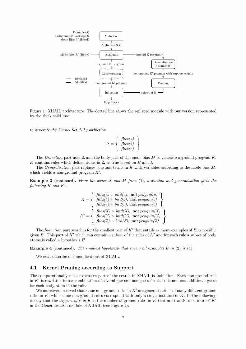
Our framework for chunking has three main parts as shown in Figure 2. Preprocessing is done usingthe Stanford CoreNLP tool from which we obtain the facts that are added to the background knowledgeof XHAIL or used with a hypothesis to predict the chunks of an input. Using XHAIL as our ILP solver welearn a hypothesis (an ASP program) from the background knowledge, mode bias, and from exampleswhich are generated using the gold-standard data. We predict chunks using our learned hypothesisand facts from preprocessing, using the Clingo (Gebser et al., 2008) ASP solver. We test by scoringpredictions against gold chunk annotations.

Example 5. An example sentence in the SemEval iSTS dataset (Agirre et al., 2016) is as follows.

Former Nazi death camp guard Demjanjuk dead at 91 (5)

The chunking present in the SemEval gold standard is as follows.

[ Former Nazi death camp guard Demjanjuk ] [ dead ] [ at 91 ] (6)

5.1 Preprocessing

Stanford CoreNLP tools (Manning et al., 2014) are used for tokenisations and POS-tagging of the input.Using a shallow parser (Bohnet et al., 2013) we obtain the dependency relations for the sentences. OurASP representation contains atoms of the following form:

9

pos (c_NNP, 1 ) . head ( 2 , 1 ) . form (1 , "Former" ) . r e l (c_NAME, 1 ) .pos (c_NNP, 2 ) . head ( 5 , 2 ) . form (2 , "Nazi" ) . r e l (c_NMOD, 2 ) .pos (c_NN, 3 ) . head ( 4 , 3 ) . form (3 , "death" ) . r e l (c_NMOD, 3 ) .pos (c_NN, 4 ) . head ( 5 , 4 ) . form (4 , "camp" ) . r e l (c_NMOD, 4 ) .pos (c_NN, 5 ) . head ( 7 , 5 ) . form (5 , "guard" ) . r e l (c_SBJ , 5 ) .pos (c_NNP, 6 ) . head ( 5 , 6 ) . form (6 , "Demjanjuk" ) . r e l (c_APPO, 6 ) .pos (c_VBD, 7 ) . head ( root , 7 ) . form (7 , "dead" ) . r e l (c_ROOT, 7 ) .pos (c_IN , 8 ) . head ( 7 , 8 ) . form (8 , " at " ) . r e l (c_ADV, 8 ) .pos (c_CD, 9 ) . head ( 8 , 9 ) . form (9 , "91" ) . r e l (c_PMOD, 9 ) .

(a) Preprocessing Output

postype (X) :− pos (X,_) .token (X) :− pos (_,X) .nextpos (P,X) :− pos (P,X+1).

(b) Background Knowledge

#modeh s p l i t (+token ) .#modeb pos ( $postype ,+ token ) .#modeb nextpos ( $postype ,+ token ) .

(c) Mode Restrictions

goodchunk (1) :− not s p l i t ( 1 ) , not s p l i t ( 2 ) , not s p l i t ( 3 ) ,not s p l i t ( 4 ) , not s p l i t ( 5 ) , s p l i t ( 6 ) .

goodchunk (7) :− s p l i t ( 6 ) , s p l i t ( 7 ) .goodchunk (8) :− s p l i t ( 7 ) , not s p l i t ( 8 ) .#example goodchunk ( 1 ) .#example goodchunk ( 7 ) .#example goodchunk ( 8 ) .

(d) Examples

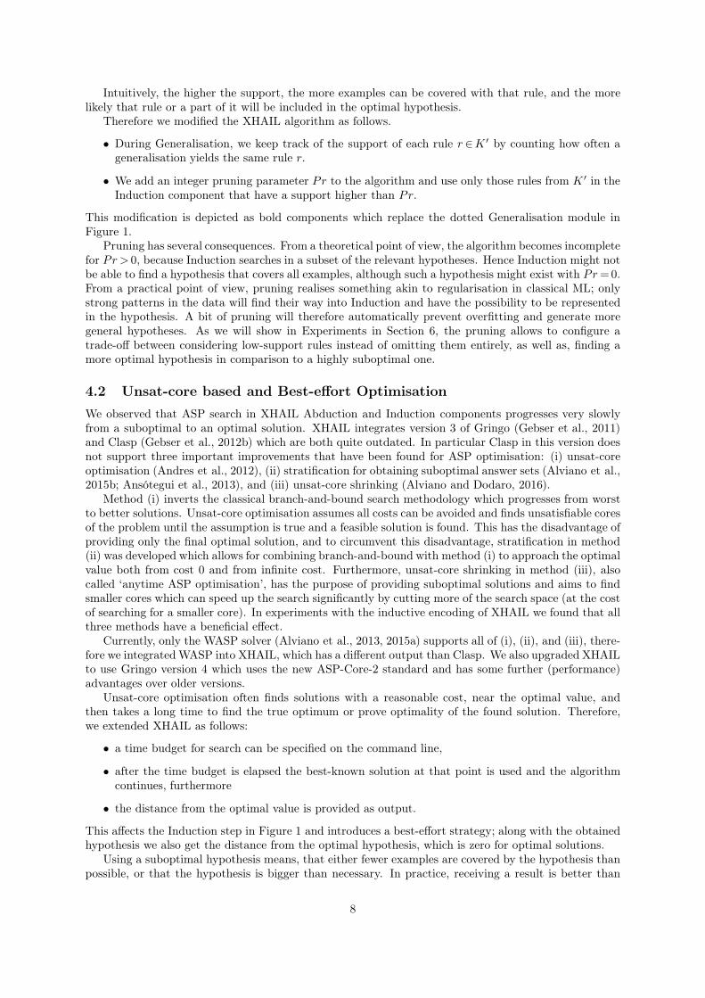
Figure 3: XHAIL input for the sentence ’Former Nazi death camp guard Demjanjuk dead at 91’ fromthe Headlines Dataset

• pos(P ,T ) which represents that token T has POS tag P ,

• form(T ,Text) which represents that token T has surface form Text ,

• head(T1 ,T2 ) and rel(R,T ) which represent that token T2 depends on token T1 with dependencyrelation R.

Example 6 (continued). Figure 3a shows the result of preprocessing performed on sentence (5), whichis a set of ASP facts.

We use Penn Treebank POS-tags as they are provided by Stanford CoreNLP. To form valid ASPconstant terms from POS-tags, we prefix them with ‘c_’, replace special characters with lowercaseletters (e.g., ‘PRP$’ becomes ‘c_PRPd’). In addition, we create specific POS-tags for punctuation (seeSection 6.4).

5.2 Background Knowledge and Mode Bias

Background Knowledge we use is shown in Figure 3b. We define which POS-tags can exist in predicatepostype/1 and which tokens exist in predicate token/1. Moreover, we provide for each token the POS-tagof its successors token in predicate nextpos/2.

Mode bias conditions are shown in Figure 3c, these limit the search space for hypothesis generation.Hypothesis rules contain as head atoms of the form

split(T )

10

which indicates, that a chunk ends at token T and a new chunk starts at token T +1. The argument ofpredicates split/1 in the head is of type token.

The body of hypothesis rules can contain pos/2 and nextpos/2 predicates, where the first argumentis a constant of type postype (which is defined in Figure 3b) and the second argument is a variable oftype token. Hence this mode bias searches for rules defining chunk splits based on POS-tag of the tokenand the next token.

We deliberately use a very simple mode bias that does not make use of all atoms in the facts obtainedfrom preprocessing. This is discussed in Section 6.5.

5.3 Learning with ILP

Learning with ILP is based on examples that guide the search. Figure 3d shows rules that recognise goldstandard chunks and #example instructions that define for XHAIL which atoms must be true to entailan example. These rules with goodchunk/1 in the head define what a good (i.e., gold standard) chunk isin each example based on where a split in a chunk occurs in the training data to help in the learning ofa hypothesis for chunking.

Note that negation is present only in these rules, although we could use it anywhere else in thebackground knowledge. Using the background knowledge, mode bias, and examples, XHAIL is then ableto learn a hypothesis.

5.4 Chunking with ASP using Learned Hypothesis

The hypothesis generated by XHAIL can then be used together with the background knowledge specifiedin Figure 3b, and with the preprocessed input of a new sentence. Evaluating all these rules yields a setof split points in the sentence, which corresponds to a predicted chunking of the input sentence.

Example 7 (continued). Given sentence (5) with token indices 1, . . . , 9, an answer set that contains theatoms {split(6), split(7)} and no other atoms for predicate split/1 yields the chunking shown in (6).

6 Evaluation and Discussion

6.1 Datasets

We are using the datasets from the SemEval 2016 iSTS Task 2 (Agirre et al., 2016), which included twoseparate files containing sentence pairs. Three different datasets were provided: Headlines, Images, andAnswers-Students. The Headlines dataset was mined by various news sources by European Media Moni-tor. The Images dataset was a collection of captions obtained from the Flickr dataset (Rashtchian et al.,2010). The Answers-Students corpus consists of the interactions between students and the BEETLE IItutorial dialogue system which is an intelligent tutoring engine that teaches students in basic electric-ity and electronics. In the following, we denote S1 and S2, by sentence 1 and sentence 2 respectively,of sentence pairs in these datasets. Regarding the size of the SemEval Training dataset, Headlines andImages datasets are larger and contained 756 and 750 sentence pairs, respectively. However, the Answers-Students dataset was smaller and contained only 330 sentence pairs. In addition, all datasets contain aTest portion of sentence pairs.

We use k-fold cross-validation to evaluate chunking with ILP, which yields k learned hypotheses andk evaluation scores for each parameter setting. We test each of these hypotheses also on the Test portionof the respective dataset. From the scores obtained this way we compute mean and standard deviation,and perform statistical tests to find out whether observed score differences between parameter settingsis statistically significant.

Table 1 shows which portions of the SemEval Training dataset we used for 11-fold cross-validation.In the following, we call these datasets Cross-Validation Sets. We chose the first 110 and 550 examplesto use for 11-fold cross-validation which results in training set sizes 100 and 500, respectively. As theAnswers-Students dataset was smaller, we merged its sentence pairs in order to obtain a Cross-ValidationSet size of 110 sentences, using the first 55 sentences from S1 and S2; and for 550 sentences, using thefirst 275 sentences from S1 and S2 each. As Test portions we only use the original SemEval Test datasetsand we always test S1 and S2 separately.

11

Dataset Cross-Validation Set Test Set

Size Examples S1 S2

H/I

100 S1 first 110 all *500 S1 first 550 all *100 S2 first 110 * all500 S2 first 550 * all

A-S100 S1 first 55 + S2 first 55 all all500 S1 first 275 + S2 first 275 all all

Table 1: Dataset partitioning for 11-fold cross-validation experiments. Size indicates the training setsize in cross-validation. Fields marked with * are not applicable, because we do not evaluate hypotheseslearned from the S1 portion of the Headlines (H) and Images (I) datasets on the (independent) S2 portionof these datasets and vice versa. For the Answers-Students (A-S) dataset we need to merge S1 and S2to obtain a training set size of 500 from the (small) SemEval Training dataset.

6.2 Scoring

We use difflib.SequenceMatcher in Python to match the sentence chunks obtained from learning in ILPagainst the gold-standard sentence chunks. From the matchings obtained this way, we compute precision,recall, and F1-score as follows.

Precision =No. of Matched Sequences

No. of ILP-learned Chunks

Recall =No. of Matched Sequences

No. of Gold Chunks

Score = 2×Precision× Recall

Precision+ Recall

To investigate the effectivity of our mode bias for learning a hypothesis that can correctly classifythe dataset, we perform cross-validation (see above) and measure correctness of all hypotheses obtainedin cross-validation also on the Test set.

Because of differences in S1/S2 portions of datasets, we report results separately for S1 and S2. Wealso evaluate classification separately for S1 and S2 for the Answers-Students dataset, although we trainon a combination of S1 and S2.

6.3 Experimental Methodology

We use Gringo version 4.5 (Gebser et al., 2011) and we use WASP version 2 (Git hash a44a95) (Alviano et al.,2015a) configured to use unsat-core optimisation with disjunctive core partitioning, core trimming, a bud-get of 30 seconds for computing the first answer set and for shrinking unsatisfiable cores with progressiveshrinking strategy. These parameters were found most effective in preliminary experiments. We configureour modified XHAIL solver to allocate a budget of 1800 seconds for the Induction part which optimisesthe hypothesis (see Section 4.2). Memory usage never exceeded 5 GB.

Tables 4–6 contains the experimental results for each Dataset, where columns Size, Pr, and So respec-tively, show the number of sentences used to learn the hypothesis, the pruning parameter for generalisingthe learned hypothesis (see Section 4.1), and the rate of how close the learned hypothesis is to the optimalresult, respectively. So is computed according to the following formula: So= Upperbound−Lowerbound

Lowerbound,

which is based on upper and lower bounds on the cost of the answer set. An So value of zero meansoptimality, and values above zero mean suboptimality; so the higher the value, the further away fromoptimality. Our results comprise of the mean and standard deviation of the F1-scores obtained from our11-fold cross-validation test set of S1 and S2 individually (column CV). Due to lack of space, we optedto leave out the scores of precision and recall, but these values show similar trends as in the Test set.For the Test sets of both S1 and S2, we include the mean and standard deviation of the Precision, Recalland F1-scores (column group T).

12

When testing machine-learning based systems, comparing results obtained on a single test set is oftennot sufficient, therefore we performed cross-validation to obtain mean and standard deviation about ourbenchmark metrics. To obtain even more solid evidence about the significance of the measured results,we additionally performed a one-tailed paired t-test to check if a measured F1 score is significantlyhigher in one setting than in another one. We consider a result significant if p < 0.05, i.e., if there isa probability of less than 5 % that the result is due to chance. Our test is one-tailed because we checkwhether one result is higher than another one, and it is a paired test because we test different parameterson the same set of 11 training/test splits in cross-validation. There are even more powerful methods forproving significance of results such as bootstrap sampling (Efron and Tibshirani, 1986), however thesemethods require markedly higher computational effort in experiments and our experiments already showsignificance with the t-test.

Rows of Tables 4–6 contain results for learning from 100 resp. 500 example sentences, and for differentpruning parameters. For both learning set sizes, we increased pruning stepwise starting from value 0until we found an optimal hypothesis (So=0) or until we saw a clear peak in classification score incross-validation (in that case, increasing the pruning is pointless because it would increase optimality ofthe hypothesis but decrease the prediction scores).

Note that datasets have been tokenised very differently, and that also state-of-the-art systems inSemEval used separate preprocessing methods for each dataset. We follow this strategy to allow a faircomparison. One example for such a difference is the Images dataset, where the ‘.’ is considered asa separate token and is later defined as a separate chunk, however in Answers-Students dataset it isintegrated onto neighboring tokens.

6.4 Results

We first discuss the results of experiments with varying training set size and varying pruning parameter,then compare our approach with the state-of-the-art systems, and finally inspect the optimal hypotheses.

Training Set Size and Pruning Parameter Tables 4–6 show results of experiments, where Tdenotes the Test portion of the respective dataset.

We observe that by increasing the size of the training set to learn the hypothesis, our scores improvedconsiderably. Due to more information being provided, the learned hypothesis can predict with higherF1 score. We also observed that for the smaller training set size (100 sentences), lower pruning numbers(in rare cases even Pr=0) resulted in achieving the optimal solution. For a bigger training set size (500sentences), without pruning the ILP procedure does not find solutions close to the optimal solution.However, by using pruning values up to Pr=10 we can reduce the size of the search space and findhypotheses closer to the optimum, which predict chunks with a higher F1 score. Our statistical testshows that, in many cases, several increments of the Pr parameter yield significantly better results, upto a point where prediction accuracy degrades because too many examples are pruned away. To selectthe best hypothesis, we increase the pruning parameter Pr until we reach the peak in the F1 score incross-validation.

Finding optimal hypotheses in the Inductive search of XHAIL (where So=0) is easily attained whenlearning from 100 sentences. For learning from 500 sentences, very higher pruning results in a trivialoptimal hypothesis (i.e., every token is a chunk) which has no predictive power, hence we do not increasePr beyond a value of 10.

Note that we never encountered timeouts in the Abduction component of XHAIL, only in the Induc-tion part. The original XHAIL tool without our improvements yields only timeouts for learning from 500examples, and few hypotheses for learning from 100 examples. Therefore we do not show these resultsin tables.

State-of-the-art comparison Table 2 shows a comparison of our results with the baseline and thethree best systems from the chunking subtask of Task 2 from SemEval2016 Task2 (Agirre et al., 2016):DTSim (Banjade et al., 2016), FBK-HLT-NLP (Magnolini et al., 2016) and runs 1 and 2 of IISCNLP(Tekumalla and Jat, 2016). We also compare with results of our own system ‘Inspire-Manual’ (Kazmi and Schüller,2016).

13

Data SystemS1 S2

P R F1 Rank P R F1 Rank

Hea

dlines

Baseline 60.5 36.6 37.6 63.6 42.5 42.8DTSim 72.5 74.3 71.3 * 72.1 74.3 70.5 *FBK-HLT-NLP 63.6 51.3 51.5 57.1 51.1 48.3IISCNLP - Run1 61.9 68.5 61.4 61.1 65.7 60.1IISCNLP - Run2 67.6 68.5 64.5 *** 71.4 71.9 68.9 **Inspire - Manual 64.5 70.4 62.4 64.3 68.4 62.2Inspire - Learned 68.1±2.5 70.6±2.5 65.4±2.6 ** 67.2±1.3 68.2±2.4 64.0±1.8 ***

Images

Baseline 19.0 15.7 16.4 13.6 17.5 13.5DTSim 77.8 77.4 77.5 * 79.5 79.1 79.2 *FBK-HLT-NLP 41.0 39.2 38.8 40.5 43.1 40.8IISCNLP - Run1 61.6 60.9 60.7 66.1 66.2 65.9IISCNLP - Run2 65.8 65.6 65.4 67.7 67.2 67.3Inspire - Manual 74.5 74.2 74.2 ** 73.8 73.6 73.6 **Inspire - Learned 66.4±15.5 74.3±0.7 73.7±0.7 *** 71.1±0.8 71.1±0.8 70.9±0.8 ***

Answ

ers-

Stu

den

ts Baseline 62.1 30.9 34.6 59.2 33.4 36.6DTSim 78.5 73.6 72.5 * 83.3 79.2 77.8 **FBK-HLT-NLP 70.3 52.5 52.8 72.4 59.1 59.3IISCNLP - Run1 67.9 63.9 60.7 *** 65.7 55.0 54.0IISCNLP - Run2 63.0 59.8 56.9 66.2 52.5 52.8Inspire - Manual 66.8 64.4 59.7 71.2 62.5 62.1 ***Inspire - Learned 66.8±2.8 70.5±2.5 63.5±2.4 ** 89.3±3.0 80.1±0.7 80.3±1.7 *

Table 2: Comparison with systems from SemEval 2016 Task 2. The number of stars shows the rank ofthe system.

• The baseline makes use of the automatic probabilistic chunker from the IXA-pipeline which providesPerceptron models (Collins, 2002) for chunking and is trained on CONLL2000 corpora and correctedmanually,

• DTSim uses a Conditional Random Field (CRF) based chunking tool using only POS-tags asfeatures,

• FBK-HLT-NLP obtains chunks using a Python implementation of MBSP chunker which uses aMemory-based part-of-speech tagger generator (Daelemans et al., 1996),

• Run 1 of IISCNLP uses OpenNLP chunker which divides the sentence into syntactically correlatedparts of words, but does not specify their internal structure, nor their role in the main sentence.Run 2 uses Stanford NLP Parser to create parse trees and then uses a perl script to create chunksbased on the parse trees, and

• Inspire-Manual (our previous system) makes use of manually set chunking rules (Abney, 1991)using ASP (Kazmi and Schüller, 2016).

Using the gold-standard chunks provided by the organisers we were able to compute the precision,recall, and F1-scores for analysis on the Headlines, Images and Answers-Students datasets.

For the scores of our system ‘Inspire-Learned’, we used the mean and average of the best configurationof our system as obtained in cross-validation experiments on the Test set and compared against the othersystems’ Test set results. Our system’s performance is quite robust: it is always scores within the topthree best systems.

Inspection of Hypotheses Table 3 shows the rules that are obtained from the hypothesis generatedby XHAIL from Sentence 1 files of all the datasets. We have also tabulated the common rules presentbetween the datasets and the extra rules which differentiate the datasets from each other. POS-tags for

14

Rules H I A-S

split(V) :- token(V), pos(c_VBD,V). X X Xsplit(V) :- token(V), nextpos(c_IN,V). X X Xsplit(V) :- token(V), nextpos(c_VBZ,V). X X Xsplit(V) :- token(V), pos(c_VB,V). X Xsplit(V) :- token(V), nextpos(c_TO,V). X Xsplit(V) :- token(V), nextpos(c_VBD,V). X Xsplit(V) :- token(V), nextpos(c_VBP,V). X Xsplit(V) :- token(V), pos(c_VBZ,V), nextpos(c_DT,V). X Xsplit(V) :- token(V), pos(c_NN,V), nextpos(c_RB,V). X Xsplit(V) :- token(V), pos(c_NNS,V). Xsplit(V) :- token(V), pos(c_VBP,V). Xsplit(V) :- token(V), pos(c_VBZ,V). Xsplit(V) :- token(V), pos(c_c,V). Xsplit(V) :- token(V), nextpos(c_POS,V). Xsplit(V) :- token(V), nextpos(c_VBN,V). Xsplit(V) :- token(V), nextpos(c_c,V). Xsplit(V) :- token(V), pos(c_PRP,V). Xsplit(V) :- token(V), pos(c_RP,V). Xsplit(V) :- token(V), pos(c_p,V). Xsplit(V) :- token(V), nextpos(c_p,V). Xsplit(V) :- token(V), pos(c_CC,V), nextpos(c_VBG,V). Xsplit(V) :- token(V), pos(c_NN,V), nextpos(c_VBD,V). Xsplit(V) :- token(V), pos(c_NN,V), nextpos(c_VBG,V). Xsplit(V) :- token(V), pos(c_NN,V), nextpos(c_VBN,V). Xsplit(V) :- token(V), pos(c_NNS,V), nextpos(c_VBG,V). Xsplit(V) :- token(V), pos(c_RB,V), nextpos(c_IN,V). Xsplit(V) :- token(V), pos(c_VBG,V), nextpos(c_DT,V). Xsplit(V) :- token(V), pos(c_VBG,V), nextpos(c_JJ,V). Xsplit(V) :- token(V), pos(c_VBG,V), nextpos(c_PRPd,V). Xsplit(V) :- token(V), pos(c_VBG,V), nextpos(c_RB,V). Xsplit(V) :- token(V), pos(c_VBZ,V), nextpos(c_IN,V). Xsplit(V) :- token(V), pos(c_EX,V). Xsplit(V) :- token(V), pos(c_RB,V). Xsplit(V) :- token(V), pos(c_VBG,V). Xsplit(V) :- token(V), pos(c_WDT,V). Xsplit(V) :- token(V), pos(c_WRB,V). Xsplit(V) :- token(V), nextpos(c_EX,V). Xsplit(V) :- token(V), nextpos(c_MD,V). Xsplit(V) :- token(V), nextpos(c_VBG,V). Xsplit(V) :- token(V), nextpos(c_RB,V). Xsplit(V) :- token(V), pos(c_IN,V), nextpos(c_NNP,V). Xsplit(V) :- token(V), pos(c_NN,V), nextpos(c_WDT,V). Xsplit(V) :- token(V), pos(c_NN,V), nextpos(c_IN,V). Xsplit(V) :- token(V), pos(c_NNS,V), nextpos(c_IN,V). Xsplit(V) :- token(V), pos(c_NNS,V), nextpos(c_VBP,V). Xsplit(V) :- token(V), pos(c_RB,V), nextpos(c_DT,V). X

Table 3: Rules in the best hypotheses obtained from training on 500 sentences (S1), where X marks thepresence of the rule in a given dataset.

punctuation are ‘c_p’ for sentence-final punctuation (‘.’, ‘?’, and ‘ !’) and ‘c_c’ for sentence-separatingpunctuation (‘,’, ‘;’, and ‘:’).

Rules which occur in all learned hypotheses can be interpreted as follows (recall the meaning ofsplit(X) from Section 5.2): (i) chunks end at past tense verbs (VBD, e.g., ‘walked’), (ii) chunks begin atsubordinating conjunctions and prepositions (IN, e.g., ‘in’), and (iii) chunks begin at 3rd person singularpresent tense verbs (VBZ, e.g., ‘walks’). Rules that are common to H and AS datasets are as follows:(i) chunks end at base forms of verbs (VB, e.g., ‘[to] walk’), (ii) chunks begin at ‘to’ prepositions (TO),and (iii) chunks begin at past tense verbs (VBD). The absence of (i) in hypotheses for the Images datasetcan be explained by the rareness of such verbs in captions of images. Note that (iii) together with thecommon rule (i) means that all VBD verbs become separate chunks in H and AS datasets. Rules thatare common to I and AS datasets are as follows: (i) chunks begin at non-3rd person verbs in presenttense (VBP, e.g., ‘[we] walk’), (ii) chunk boundaries are between a determiner (DT, e.g., ‘both’) and a

15

3rd person singular present tense verb (VBZ), and (iii) chunk boundaries are between adverbs (RB, e.g.,‘usually’) and common, singular, or mass nouns (NN, e.g., ‘humor’). Interestingly, there are no rulescommon to H and I datasets except for the three rules mutual to all three datasets.

For rules occurring only in single datasets, we only discuss a few interesting cases in the following.Rules that are unique to the Headlines dataset include rules which indicate that the sentence separators‘,’, ‘;’, and ‘:’, become single chunks, moreover chunks start at genitive markers (POS, ‘’s’). Both isnot the case for the other two data sets. Rules unique to the Images dataset include that sentence-final punctuation (‘.’, ‘?’, and ‘ !’) become separate chunks, rules for chunk boundaries between verb(VB_) and noun (NN_) tokens, and chunk boundaries between possessive pronouns (PRP$, encodedas ‘c_PRPd’, e.g., ‘their’) and participles/gerunds (VBG, e.g., ‘falling’). Rules unique to Answers-Students dataset include chunks containing ‘existential there’ (EX), adverb tokens (RB), gerunds (VBG),and several rules for splits related to WH-determiners (WDT, e.g., ‘which’), WH-adverbs (WRB, e.g.,‘how’), and prepositions (IN).

We see that learned hypotheses are interpretable, which is not the case in classical machine learningtechniques such as Neural Networks (NN), Conditional Random Fields (CRF), and Support VectorMachines (SVM).

6.5 Discussion

We next discuss the potential impact of our approach in NLP and in other applications, outline thestrengths and weaknesses, and discuss reasons for several design choices we made.

Impact and Applicability ILP is applicable to many problems of traditional machine learning, butusually only applicable for small datasets. Our addition of pruning enables learning from larger datasetsat the cost of obtaining a more coarse-grained hypothesis and potentially suboptimal solutions.

The main advantage of ILP is interpretability and that it can achieve good results already with smalldatasets. Interpretability of the learned rule-based hypothesis makes the learned hypothesis transparentas opposed to black-box models of other approaches in the field such as Conditional Random Fields,Neural Networks, or Support Vector Machines. These approaches are often purely statistical, operate onbig matrices of real numbers instead of logical rules, and are not interpretable. The disadvantage of ILPis that it often does not achieve the predictive performance of purely statistical approaches because thecomplexity of ILP learning limits the number of distinct features that can be used simultaneously.

Our approach allows finding suboptimal hypotheses which yield a higher prediction accuracy thanan optimal hypothesis trained on a smaller training set. Learning a better model from a larger datasetis exactly what we would expect in machine learning. Before our improvement of XHAIL, obtaining anyhypothesis from larger datasets was impossible: the original XHAIL tool does not return any hypothesiswithin several hours when learning from 500 examples.

Our chunking approach learns from a small portion of the full SemEval Training dataset, basedon only POS-tags, but it still achieves results close to the state-of-the-art. Additionally it provides aninterpretable model that allowed us to pinpoint non-uniform annotation practices in the three datasets ofthe SemEval 2016 iSTS competition. These observations give direct evidence for differences in annotationpractice for three datasets with respect to punctuation and genitives, as well as differences in the contentof the datasets

Strengths and weaknesses Our additions of pruning and the usage of suboptimal answer sets makeILP more robust because it permits learning from larger datasets and obtaining (potentially suboptimal)solutions faster.

Our addition of a time budget and usage of suboptimal answer sets is a purely beneficial addition tothe XHAIL approach. If we disregard the additional benefits of pruning, i.e., if we disable pruning bysetting Pr=0, then within the same time budget, the same optimal solutions are to be found as if usingthe original XHAIL approach. In addition, before finding the optimal solution, suboptimal hypothesesare provided in an online manner, together with information about their distance from the optimalsolution.

The strength of pruning before the Induction phase is, that it permits learning from a bigger set ofexamples, while still considering all examples in the dataset. A weakness of pruning is, that a hypothesis

16

which fits perfectly to the data might not be found anymore, even if the mode bias could permit such aperfect fit. In NLP applications this is not a big disadvantage, because noise usually prevents a perfect fitanyways, and overfitting models is indeed often a problem. However, in other application domains suchas learning to interpret input data from user examples (Gulwani et al., 2015), a perfect fit to the inputdata might be desired and required. Note that pruning examples to learn from inconsistent data as doneby Tang and Mooney (Tang and Mooney, 2001) is not necessary for our approach. Instead, non-coveredexamples incur a cost that is optimised to be as small as possible.

Design decisions In our study, we use a simple mode bias containing only the current and next POStags, which is a deliberate choice to make results easier to compare. We performed experiments withadditional body atoms head/2 and rel/2 in the body mode bias, moreover with negation in the bodymode bias. However, these experiments yielded significantly larger hypotheses with only small increasesin accuracy. Therefore we here limit the analysis to the simple case and consider more complex modebiases as future work. Note that the best state-of-the-art system (DTSim) is a CRF model solely basedon POS-tags, just as our hypothesis is only making use of POS-tags. By considering more than thecurrent and immediately succeeding POS tag, DTSim can achieve better results than we do.

The representation of examples is an important part of our chunking case as described in Section 5.We define predicate goodchunk with rules that consider presence and absence of splits for each chunk. Wemake use of the power of NAF in these rules. We also experimented with an example representation thatjust gave all desired splits as #example split(X) and all undesired splits as #example not split(Y).This representation contains an imbalance in the split versus not split class, moreover, chunks are notrepresented as a concept that can be optimised in the inductive search for the best hypothesis. Hence,it is not surprising that this simpler representation of examples gave drastically worse scores, and we donot report any of these results in detail.

7 Conclusion and Future Work

Inductive Logic Programming combines logic programming and machine learning, and it provides inter-pretable models, i.e., logical hypotheses, which are learned from data. ILP has been applied to a varietyof NLP and other problems such as parsing (Tang and Mooney, 2001; Zelle and Mooney, 1996), auto-matic construction of biological knowledge bases from scientific abstracts (Craven and Kumlien, 1999),automatic scientific discovery (King et al., 2004), and in Microsoft Excel Gulwani et al. (2015) whereusers can specify data extraction rules using examples. Therefore, ILP research has the potential forbeing used in a wide range of applications.

In this work, we explored the usage of ILP for the NLP task of chunking and extend the XHAIL ILPsolver to increase its scalability and applicability for this task. Results indicate that ILP is competitive tostate-of-the-art ML techniques for this task and that we successfully extended XHAIL to allow learningfrom larger datasets than previously possible. Learning a hypothesis using ILP has the advantage of aninterpretable representation of the learned knowledge, such that we know exactly which rule has beenlearned by the program and how it affects our NLP task. In this study, we also gain insights about thedifferences and common points of datasets that we learned a hypothesis from. Moreover, ILP permitslearning from small training sets where techniques such as Neural Networks fail to provide good results.

As a first contribution to the ILP tool XHAIL we have upgraded the software so that it uses the newestsolver technology, and that this technology is used in a best-effort manner that can utilise suboptimalsearch results. This is effective in practice, because finding the optimal solution can be disproportionatelymore difficult than finding a solution close to the optimum. Moreover, the ASP technique we use hereprovides a clear information about the degree of suboptimality. During our experiments, a new version ofClingo was published which contains most techniques in WASP (except for core shrinking). We decidedto continue using WASP for this study because we saw that core shrinking is also beneficial to search.Extending XHAIL to use Clingo in a best-effort manner is quite straight-forward.

As a second contribution to XHAIL we have added a pruning parameter to the algorithm thatallows fine-tuning the search space for hypotheses by filtering out rule candidates that are supportedby fewer examples than other rules. This addition is a novel contribution to the algorithm, which leadsto significant improvements in efficiency, and increases the number of hypotheses that are found in agiven time budget. While pruning makes the method incomplete, it does not reduce expressivity. The

17

hypotheses and background knowledge may still contain unrestricted Negation as Failure. Pruning inour work is similar to the concept of the regularisation in ML and is there to prevent overfitting inthe hypothesis generation. Pruning enables the learning of logical hypotheses with dataset sizes thatwere not feasible before. We experimentally observed a trade-off between finding an optimal hypothesisthat considers all potential rules on one hand, and finding a suboptimal hypothesis that is based onrules that are supported by few examples. Therefore the pruning parameter has to be adjusted on anapplication-by-application basis.

Our work has focused on providing comparable results to ML techniques and we have not utilised thefull power of ILP with NAF in rule bodies and predicate invention. As future work, we plan to extendthe predicates usable in hypotheses to provide a more detailed representation of the NLP task, moreoverwe plan to enrich the background knowledge to aid ILP in learning a better hypothesis with a deeperstructure representing the boundaries of chunks.

We provide the modified XHAIL system in a public repository fork (Bragaglia and Schüller, 2016).

Acknowledgments

This research has been supported by the Scientific and Technological Research Council of Turkey(TUBITAK) [grant number 114E777] and by the Higher Education Commission of Pakistan (HEC).We are grateful to Carmine Dodaro for providing us with support regarding the WASP solver.

References

Abney, S. P. (1991). Parsing by chunks. In Principle-based parsing, pages 257–278.

Agirre, E., Gonzalez-Agirre, A., Lopez-Gazpio, I., Maritxalar, M., Rigau, G., and Uria, L. (2016).SemEval-2016 task 2: Interpretable Semantic Textual Similarity. In Proceedings of SemEval, pages512–524.

Alviano, M. and Dodaro, C. (2016). Anytime answer set optimization via unsatisfiable core shrinking.Theory and Practice of Logic Programming, 16(5-6):533–551.

Alviano, M., Dodaro, C., Faber, W., Leone, N., and Ricca, F. (2013). WASP: A native ASP solver basedon constraint learning. In Logic Programming and Nonmonotonic Reasoning, pages 54–66.

Alviano, M., Dodaro, C., Leone, N., and Ricca, F. (2015a). Advances in WASP. In Logic Programmingand Nonmonotonic Reasoning , pages 40–54.

Alviano, M., Dodaro, C., Marques-Silva, J., and Ricca, F. (2015b). Optimum stable model search:algorithms and implementation. Journal of Logic and Computation, page exv061.

Andres, B., Kaufmann, B., Matheis, O., and Schaub, T. (2012). Unsatisfiability-based optimization inclasp. In International Conference on Logic Programming, Technical Communications, pages 212–221.

Ansótegui, C., Bonet, M. L., and Levy, J. (2013). SAT-based MaxSAT algorithms. Artificial Intelligence,196:77–105.

Banjade, R., Maharjan, N., Niraula, N. B., and Rus, V. (2016). DTSim at SemEval-2016 task 2:Interpreting Similarity of Texts Based on Automated Chunking, Chunk Alignment and SemanticRelation Prediction. In Proceedings of SemEval, pages 809–813.

Bohnet, B., Nivre, J., Boguslavsky, I., Farkas, R., Ginter, F., and Hajič, J. (2013). Joint morphologicaland syntactic analysis for richly inflected languages. Transactions of the Association for ComputationalLinguistics, 1:415–428.

Bragaglia, S. and Schüller, P. (2016). XHAIL (Version 4c5e0b8) [System for eXtended Hybrid AbductiveInductive Learning]. Retrieved from https://github.com/knowlp/XHAIL.

Brewka, G., Eiter, T., and Truszczyński, M. (2011). Answer set programming at a glance. Communica-tions of the ACM, 54(12):92–103.

Calimeri, F., Faber, W., Gebser, M., Ianni, G., Kaminski, R., Krennwallner, T., Leone, N., Ricca, F.,

18

and Schaub, T. (2012). ASP-Core-2 Input language format. Technical report, ASP StandardizationWorking Group.

Clocksin, W. and Mellish, C. S. (2003). Programming in PROLOG. Springer Science & Business Media.

Collins, M. (2002). Discriminative training methods for hidden markov models: Theory and experimentswith perceptron algorithms. In Proceedings of the ACL-02 conference on Empirical methods in naturallanguage processing-Volume 10, pages 1–8. Association for Computational Linguistics.

Craven, M. and Kumlien, J. (1999). Constructing biological knowledge bases by extracting informationfrom text sources. In International Conference on Intelligent Systems for Molecular Biology (ISMB),pages 77–86.

Cussens, J. (2001a). Integrating probabilistic and logical reasoning. In Foundations of Bayesianism,pages 241–260.

Cussens, J. (2001b). Parameter estimation in stochastic logic programs. Machine Learning, 44(3):245–271.

Daelemans, W., Zavrel, J., Berck, P., and Gillis, S. (1996). Mbt: A memory-based part of speechtagger-generator. arXiv preprint cmp-lg/9607012.

De Raedt, L. (1997). Logical settings for concept-learning. Artificial Intelligence, 95(1):187–201.

De Raedt, L. and Kersting, K. (2008). Probabilistic inductive logic programming. In ProbabilisticInductive Logic Programming, pages 1–27.

Dumais, S., Platt, J., Heckerman, D., and Sahami, M. (1998). Inductive learning algorithms and represen-tations for text categorization. In Proceedings of the Seventh International Conference on Informationand Knowledge Management, pages 148–155.

Efron, B. and Tibshirani, R. (1986). Bootstrap Methods for Standard Errors, Confidence Intervals, andOther Measures of Statistical Accuracy. Statistical Science, 1(1):54–75.

Erdem, E., Gelfond, M., and Leone, N. (2016). Applications of Answer Set Programming. AI Magazine,37(3):53–68.

Gebser, M., Kaminski, R., Kaufmann, B., Ostrowski, M., Schaub, T., and Thiele, S. (2008). A user’sguide to gringo, clasp, clingo, and iclingo. Technical report, University of Potsdam.

Gebser, M., Kaminski, R., Kaufmann, B., and Schaub, T. (2012a). Answer set solving in practice.Synthesis Lectures on Artificial Intelligence and Machine Learning, 6(3):1–238.

Gebser, M., Kaminski, R., König, A., and Schaub, T. (2011). Advances in gringo series 3. In InternationalConference on Logic Programming and Non-monotonic Reasoning, pages 345–351.

Gebser, M., Kaufmann, B., and Schaub, T. (2012b). Conflict-driven answer set solving: From theory topractice. Artificial Intelligence, 187:52–89.

Gelfond, M. and Lifschitz, V. (1988). The Stable Model Semantics for Logic Programming. In Interna-tional Conference and Symposium on Logic Programming, pages 1070–1080.

Gulwani, S., Hernandez-Orallo, J., Kitzelmann, E., Muggleton, S. H., Schmid, U., and Zorn, B. (2015).Inductive programming meets the real world. Communications of the ACM, 58(11):90–99.

Kakas, A. C., Kowalski, R. A., and Toni, F. (1992). Abductive Logic Programming. Journal of Logicand Computation, 2(6):719–770.

Katzouris, N., Artikis, A., and Paliouras, G. (2015). Incremental learning of event definitions withinductive logic programming. Machine Learning, 100(2-3):555–585.

Kazmi, M. and Schüller, P. (2016). Inspire at SemEval-2016 task 2: Interpretable semantic textualsimilarity alignment based on answer set programming. In Proceedings of SemEval, pages 1109–1115.

King, R. D., Whelan, K. E., Jones, F. M., Reiser, P. G. K., Bryant, C. H., Muggleton, S. H., Kell, D. B.,and Oliver, S. G. (2004). Functional genomic hypothesis generation and experimentation by a robotscientist. Nature, 427(6971):247–252.

Kitzelmann, E. (2009). Inductive programming: A survey of program synthesis techniques. In Interna-tional Workshop on Approaches and Applications of Inductive Programming, pages 50–73.

19

Law, M., Russo, A., and Broda, K. (2014). Inductive learning of answer set programs. In EuropeanWorkshop on Logics in Artificial Intelligence, pages 311–325.

Law, M., Russo, A., and Broda, K. (2015). Learning weak constraints in answer set programming.Theory and Practice of Logic Programming, 15(4-5):511–525.

Lifschitz, V. (2002). Answer set programming and plan generation. Artificial Intelligence, 138(1-2):39–54.

Lloyd, J. W. (2012). Foundations of logic programming. Springer Science & Business Media.

Magnolini, S., Feltracco, A., and Magnini, B. (2016). FBK-HLT-NLP at SemEval-2016 task 2: Amultitask, deep learning approach for interpretable semantic textual similarity. In Proceedings ofSemEval, pages 783–789.

Manning, C. D. and Schütze, H. (1999). Foundations of statistical natural language processing (Vol.999). Cambridge:MIT Press.

Manning, C. D., Surdeanu, M., Bauer, J., Finkel, J. R., Bethard, S., and McClosky, D. (2014). TheStanford CoreNLP natural language processing toolkit. In ACL System Demonstrations, pages 55–60.

Mitra, A. and Baral, C. (2016). Addressing a question answering challenge by combining statisticalmethods with inductive rule learning and reasoning. In Association for the Advancement of ArtificialIntelligence, pages 2779–2785.

Mooney, R. J. (1996). Inductive logic programming for natural language processing. In Inductive LogicProgramming, pages 1–22.

Muggleton, S. (1991). Inductive logic programming. New generation computing, 8(4):295–318.

Muggleton, S. (1995). Inverse entailment and Progol. New generation computing, 13(3-4):245–286.

Muggleton, S. (1999). Inductive logic programming: issues, results and the challenge of learning languagein logic. Artificial Intelligence, 114(1-2):283–296.

Muggleton, S. (2002). Learning structure and parameters of stochastic logic programs. In InternationalConference on Inductive Logic Programming, pages 198–206.

Muggleton, S. and Buntine, W. (1992). Machine invention of first-order predicates by inverting resolution.In Proceedings of the Fifth International Conference on Machine Learning, pages 339–352.

Muggleton, S. and De Raedt, L. (1994). Inductive logic programming: Theory and methods. The Journalof Logic Programming, 19:629–679.

Muggleton, S., De Raedt, L., Poole, D., Bratko, I., Flach, P., Inoue, K., and Srinivasan, A. (2012). ILPturns 20. Machine Learning, 86(1):3–23.

Muggleton, S. et al. (1996). Stochastic logic programs. Advances in Inductive Logic Programming,32:254–264.

Muggleton, S., Feng, C., et al. (1990). Efficient induction of logic programs. The Turing Institute.

Muggleton, S. H., Lin, D., Pahlavi, N., and Tamaddoni-Nezhad, A. (2014). Meta-interpretive learning:application to grammatical inference. Machine Learning, 94(1):25–49.

Plotkin, G. D. (1970). A note on inductive generalization. Machine intelligence, 5(1):153–163.

Plotkin, G. D. (1971). A further note on inductive generalization. Machine intelligence, 6:101–124.

Quinlan, J. R. (1990). Learning logical definitions from relations. Machine Learning, 5(3):239–266.

Rashtchian, C., Young, P., Hodosh, M., and Hockenmaier, J. (2010). Collecting image annotations usingAmazon’s Mechanical Turk. In Proceedings of the NAACL HLT 2010 Workshop on Creating Speechand Language Data with Amazon’s Mechanical Turk, pages 139–147.

Ray, O. (2009). Nonmonotonic abductive inductive learning. Journal of Applied Logic, 7(3):329–340.

Sammut, C. and Banerji, R. B. (1986). Learning concepts by asking questions. Machine Learning: Anartificial intelligence approach, 2:167–192.

Sato, T., Kameya, Y., and Zhou, N.-F. (2005). Generative modeling with failure in PRISM. In Interna-tional Joint Conference on Artificial Intelligence, pages 847–852.

20

Schüller, P. (2013). Flexible Combinatory Categorial Grammar Parsing using the CYK Algorithm andAnswer Set Programming. In International Conference on Logic Programming and Non-monotonicReasoning, pages 499–511.

Schüller, P. (2014). Tackling Winograd Schemas by Formalizing Relevance Theory in Knowledge Graphs.In International Conference on Principles of Knowledge Representation and Reasoning (KR), pages358–367. AAAI Press.

Schüller, P. (2016). Modeling Variations of First-Order Horn Abduction in Answer Set Programming.Fundamenta Informaticae, 149:159–207.

Schwitter, R. (2012). Answer Set Programming via Controlled Natural Language Processing. In Con-trolled Natural Language, pages 26–43.

Shapiro, E. Y. (1983). Algorithmic program debugging. MIT press.

Sharma, A., Vo, N. H., Aditya, S., and Baral, C. (2015). Towards addressing the winograd schemachallenge - Building and using a semantic parser and a knowledge hunting module. In InternationalJoint Conference on Artificial Intelligence (IJCAI), pages 1319–1325.

Srinivasan, A. (2001). The aleph manual. Retrieved fromhttp://www.cs.ox.ac.uk/activities/machinelearning/Aleph/aleph.html.

Tang, L. R. and Mooney, R. J. (2001). Using multiple clause constructors in inductive logic programmingfor semantic parsing. In European Conference on Machine Learning, pages 466–477.

Tekumalla, L. and Jat, S. (2016). IISCNLP at SemEval-2016 task 2: Interpretable STS with ILP basedMultiple Chunk Aligner. In Proceedings of SemEval, pages 790–795.

Tjong Kim Sang, E. F. and Buchholz, S. (2000). Introduction to the CoNLL-2000 shared task: Chunking.In Workshop on Learning Language in Logic and Conference on Computational Natural LanguageLearning, pages 127–132.

Wirth, R. (1989). Completing logic programs by inverse resolution. In European Working Session onLearning, pages 239–250.

Zelle, J. M. and Mooney, R. J. (1996). Learning to parse database queries using inductive logic program-ming. In Proceedings of the National Conference on Artificial Intelligence, pages 1050–1055.

Zelle, J. M., Mooney, R. J., and Konvisser, J. B. (1994). Combining top-down and bottom-up techniquesin inductive logic programming. In Proceedings of the Eleventh International Conference on MachineLearning, pages 343–351.

21

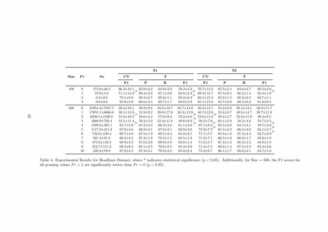
S1 S2

Size Pr So CV T CV T

F1 P R F1 F1 P R F1

100 0 172.8±46.2 66.3±10.1 63.0±2.2 64.9±3.3 59.4±3.3 70.7±14.2 65.5±2.4 64.6±2.7 60.5±2.61 10.9±5.0 71.1±13.3

|* 69.4±2.0 67.1±2.0 63.8±2.2|* 69.3±15.7 67.3±0.5 66.2±1.4 62.4±1.0

|*

2 0.3±0.8 73.1±8.0 69.3±0.7 69.2±1.1 65.0±0.4|* 66.5±15.4 65.9±1.5 68.2±0.5 62.7±1.1

3 0.0±0.0 65.9±5.9 66.6±3.4 69.7±1.7 63.0±2.9 65.1±15.6 64.7±0.9 68.5±0.3 61.6±0.5

500 0 31954.4±7057.7 39.4±18.1 50.9±9.8 34.8±18.7 35.7±14.0 39.2±12.7 53.2±8.0 38.4±14.1 38.9±11.71 17855.1±6866.0 39.1±14.9 51.9±9.2 39.0±17.9 38.3±13.9 40.7±12.6 53.4±8.7 40.0±14.7 39.7±11.92 6238.5±1530.8 55.8±10.5

|* 59.6±4.2 57.0±9.2 53.2±6.8|* 53.0±14.3

|* 59.4±5.7 52.0±11.9 49.4±9.53 4260.9±792.4 52.5±11.4 59.2±5.0 52.4±11.8 49.6±9.3

|* 59.2±7.8 62.1±2.9 58.5±4.6 54.7±3.54 1598.6±367.1 65.7±3.8

|* 65.2±3.3 66.3±3.0 61.1±3.0|* 67.1±8.4

|* 63.3±2.0 64.7±4.1 59.7±3.0|*

5 1117.2±211.3 67.0±4.6 66.8±3.1 67.8±3.1 62.9±3.0 73.3±7.3|* 65.5±2.3 66.4±3.6 62.1±2.7

|*

6 732.6±130.4 69.7±4.0 67.5±1.9 69.5±2.4 64.3±2.1 71.7±5.7 65.3±1.6 67.4±4.4 62.7±2.9|*

7 561.4±81.8 68.2±4.5 67.2±1.9 70.5±1.5 64.5±1.8 71.2±7.1 66.5±1.0 68.0±1.7 63.6±1.08 475.0±142.3 68.9±4.5 67.0±2.6 69.0±5.8 63.8±4.4 71.8±5.7 67.2±1.3 68.2±2.4 64.0±1.89 312.7±111.2 69.3±6.2 68.1±2.5 70.6±2.5 65.4±2.6 71.2±5.5 66.6±1.4 67.5±2.3 63.3±2.010 220.3±59.9 67.8±4.5 67.3±2.1 70.9±2.8 65.0±2.4 73.4±6.7 66.1±1.7 68.6±2.1 63.7±1.6

Table 4: Experimental Results for Headlines Dataset, where * indicates statistical significance (p < 0.05). Additionally, for Size = 500, the F1 scores forall pruning values Pr > 1 are significantly better than Pr = 0 (p < 0.05).

22

S1 S2

Size Pr So CV T CV T

F1 P R F1 F1 P R F1

100 0 0.5±1.0 81.8±12.7 66.4±15.5 74.3±0.7 73.7±0.7 73.9±0.7 60.1±9.5 60.1±9.6 60.1±9.51 0.0±0.0 80.9±14.4 64.5±10.8 72.7±1.4 72.1±1.4 72.3±1.4 50.2±5.6 50.0±5.6 50.1±5.62 0.0±0.0 78.2±15.3 64.5±13.7 69.2±1.4 68.9±0.8 68.9±1.2 47.5±1.8 47.3±1.8 47.4±1.83 0.0±0.0 72.7±14.2 66.4±16.7 67.0±0.5 67.8±0.5 67.1±0.5 47.3±1.5 47.1±1.5 47.2±1.5

500 0 3797.3±1019.9 47.6±8.6 45.9±12.5 47.1±8.8 46.2±8.9 46.4±8.9 45.0±12.9 45.5±12.8 44.6±13.21 670.1±153.1 64.2±8.2

|* 68.1±7.4 57.1±11.1 56.1±11.1|* 56.4±11.1

|* 63.1±9.2 63.1±9.5 62.9±9.4|*

2 286.2±90.2 69.5±4.9|* 73.8±7.1 66.4±6.6 65.6±6.6

|* 65.8±6.6|* 68.4±6.0 68.4±6.0 68.2±6.0

|*

3 159.1±36.4 70.9±6.8 70.1±7.0 66.0±7.6 65.4±7.8 65.4±7.7 69.8±3.7 69.7±3.6 69.6±3.74 83.4±25.8 74.7±5.7 68.8±6.4 70.2±2.0 69.6±1.9 69.7±1.9 67.0±7.2 66.7±7.2 66.7±7.25 23.8±11.0 74.2±6.6 70.7±4.7 71.9±1.5 71.1±1.4

|* 71.3±1.4 71.0±1.7 70.9±1.8 70.8±1.86 10.8±4.5 75.3±5.9 73.2±4.5 71.7±0.4 71.0±0.4 71.2±0.4 71.1±0.8 71.1±0.8 70.9±0.87 3.4±3.6 74.4±5.9 72.1±4.2 71.2±0.3 70.5±0.3 70.7±0.3 69.7±1.4 69.7±1.4 69.6±1.48 1.5±1.4 74.5±5.3 72.3±5.8 71.2±0.0 70.4±0.0 70.6±0.0 68.6±0.8 68.6±0.7 68.4±0.79 1.2±1.4 74.5±5.3 71.9±5.8 71.2±0.0 70.4±0.0 70.6±0.0 68.4±0.5 68.3±0.5 68.2±0.510 0.7±0.8 74.2±5.2 71.8±5.5 70.9±0.9 70.1±0.9 70.4±0.9 68.6±0.0 68.5±0.0 68.3±0.0

Table 5: Experimental Results for Images Dataset, where * indicates statistical significance (p < 0.05). Additionally, for Size = 500, the F1 scores for allpruning values Pr > 0 are significantly better than Pr = 0 (p < 0.05).

23

S1+S2 S1 S2

Size Pr So CV T T

F1 P R F1 P R F1

100 0 93.2±22.6 66.1±12.9 69.3±1.5 63.2±3.2 61.0±2.6 89.3±3.0 80.1±0.7 80.3±1.71 5.3±4.6 67.0±11.5 67.9±1.3 61.6±1.8 59.4±1.7 87.7±1.0 79.7±0.8 79.5±1.02 0.0±0.0 65.0±10.8 67.7±0.7 64.9±1.4 61.2±0.8 86.3±1.5 80.2±0.5 78.4±1.43 0.0±0.0 64.8±10.4 66.8±0.4 63.0±1.4 59.9±0.5 86.6±1.5 80.7±0.3 78.9±1.4

500 0 20723.5±3996.9 36.3±10.6 54.2±5.5 39.8±13.2 38.7±9.9 51.2±10.8 37.2±15.0 36.0±12.41 6643.4±1131.1 49.3±8.7

|* 60.0±4.9 51.3±10.1 48.7±7.2 62.9±9.9 53.4±15.6 52.1±13.8|*

2 4422.2±734.7 54.5±9.7 62.6±2.4 60.6±8.1 56.1±5.5|* 66.4±7.0 59.9±11.7 57.6±10.8

|*

3 2782.2±626.9 57.5±10.6 62.2±3.0 62.4±8.7 56.7±5.7 67.6±10.8 62.2±15.5 59.4±14.54 1541.6±311.3 65.5±4.1

|* 66.8±2.8 70.5±2.5 63.5±2.4|* 78.9±2.0 79.5±2.0 76.0±2.0

|*

5 1072.4±155.5 63.6±7.8 66.1±2.7 67.6±5.1 61.7±3.5 80.8±3.4 77.1±3.3 74.5±3.06 789.1±158.0 64.8±6.5 65.5±1.9 64.2±4.9 59.4±3.6 83.3±2.7 75.9±4.0 74.4±3.37 634.7±184.0 66.3±7.8 65.9±2.2 64.6±3.5 59.7±2.6 82.9±3.4 75.2±5.2 74.2±4.08 449.8±87.4 63.9±6.6 65.0±2.5 64.5±6.5 59.1±4.5 80.3±4.4 74.2±8.2 72.2±6.89 317.0±89.7 63.9±6.4 64.1±2.4 64.3±4.0 58.3±3.4 82.3±4.3 74.9±5.5 72.9±5.310 225.5±45.7 63.4±5.1 66.6±1.7 65.3±2.6 60.1±1.8 82.4±5.2 74.1±8.0 72.7±7.4

Table 6: Experimental Results for Answers-Students Dataset, where * indicates statistical significance (p < 0.05). Additionally, for Size = 500, the F1scores for all pruning values Pr > 0 are significantly better than Pr = 0 (p < 0.05).

24