1

INDUCTIVE ASPECTS OF CONFIRMATION, INFORMATION, AND CONTENT

Contribution to Schilpp-volume The Philosophy of Jaakko Hintikka

Theo A.F. Kuipers

Introduction

This contribution consists of three parts. In Section 1, which is a kind of summary of Part I of (Kuipers,2000), I will characterize Hintikka's quantitative theory of confirmation as one of the four main ones.Moreover, I will disentangle the structural and genuine inductive aspects in these theories ofconfirmation. In Section 2 I will make a start with further developing Hintikka's ideas (Hintikka, 1968)about two major types of information, by him called information and content. In (Hintikka, 1997) hewrote "In hindsight, I regret that I did not develop further the ideas presented in Hintikka (1968)". I willpoint out the close relation between transmitted information and content on the one hand andconfirmation on the other. Moreover, I will characterize Hintikka's aims and claims regarding the choicebetween hypotheses when dealing with explanation and generalization in relation to (transmitted)information and content. In Section 3 I will first disentangle the structural and genuine inductive aspectsof prior and posterior probabilities and of transmitted information and content. Then I will discussHintikka's answers to the question of what to maximize in the service of explanation and generalization,viz. maximizing information by maximizing likelihood and maximizing (transmitted) content,respectively. I will suggest alternative answers, viz. in terms of structural and inductive aspects,respectively. I will conclude with some remarks about the choice of a probability function, a problem thattends to remain hidden when dealing with the choice between hypotheses on the basis of a fixedprobability function underlying a theory of confirmation.

1. Ordering the landscape of confirmation

The aim of this section is to give a coherent survey of qualitative and quantitative notions of confirmation,partly by synthesizing the work of others, in a standard or non-standard way, partly by taking distance tothe work of others. It starts with qualitative, more specifically, deductive confirmation, of which thestandard form is supplemented with two comparative principles. Keeping deductive confirmation asextreme partial explication in mind, it then turns to quantitative, more specifically, probabilisticconfirmation, and introduces the crucial distinction between inductive and non-inductive, or structural,confirmation. This will lead to a survey of the four main theories of confirmation for universalhypotheses, viz. those of Popper, Carnap, Bayes and Hintikka. Finally, the section deals with the questionof a general (quantitative) degree of confirmation and its decomposition into degrees of structural andinductive confirmation, leading to four kinds of inductive confirmation.

2

1.1. Types of confirmation1.1.1. Deductive confirmationContrary to many critics, and partly in line with Gemes (1990), I believe that the notion of deductive (d-)confirmation makes perfectly good sense as partial explication, provided the classificatory definition issupplemented with some comparative principles. More specifically, "(contingent) evidence E d-confirms(consistent) hypothesis H" is defined by the clause: H (logically) entails E, and further obeys the followingprinciples:

Comparative principles:P1: if H entails E and E entails E* (and not vice versa) then E d-confirms H more than E* .P2: if H and H* both entail E then E d-confirms H and H* equally.

To be sure, this definition-with-comparative-supplement only makes sense as a partial explication of theintuitive notion of confirmation; it leaves room for non-deductive, in particular, probabilistic extensions,as we will see below. However, let us first look more closely at the comparative principles. They are veryreasonable in the light of the fact that the deductive definition can be conceived as a (deductive) successdefinition of confirmation: if H entails E, E clearly is a success of H, if not a predictive success, then atleast a kind of explanatory success. From this perspective, P1 says that a stronger (deductive) successconfirms a hypothesis more than a weaker one, and P2 says that two hypotheses should be equally praisedfor the same success. In particular P2 runs against standard conceptions. However, in Chapter 2 of(Kuipers, 2000) I deal extensively with the possible objections and show, moreover, that the presentanalysis can handle the confirmation paradoxes discovered by Hempel and Goodman. Deductive confirmation can also be supplemented with 'conditional deductive confirmation': E d-confirms H, assuming a condition C, that is, H&C entails E. This type of conditionalization, alsoapplicable for non-deductive confirmation will further be neglected in this survey.

1.1.2. Probabilistic confirmationProbabilistic confirmation presupposes, by definition, a probability function, indicated by p, that is, a real-valued function obeying the standard axioms of probability, which may nevertheless be of one kind oranother (see below). But first I will briefly deal with the general question of a probabilistic criterion ofconfirmation. The standard (or forward) criterion for probabilistic confirmation is that the posteriorprobability p(H|E) exceeds the (relative to the background knowledge) prior probability p(H), that is,p(H|E) > p(H). However, this criterion is rather inadequate for 'p-zero' hypotheses. For example, if p(H)=0and E d-confirms H, this confirmation cannot be seen as an extreme case of probabilistic confirmation,since p(H|E)=p(H)=0. However, for p-non-zero hypotheses and assuming 0<p(E)<1, the standard criterionis equivalent to the backward or success criterion, according to which the so-called likelihood p(E|H)exceeds the initial probability p(E) of E: p(E|H) > p(E). Now it is easy to check that any probabilityfunction respects d-confirmation according to this criterion, since p(E|H) = 1 when H entails E, and hence

3

exceeds p(E), even if p(H)=0. More generally, the success criterion can apply in all p-zero cases in whichp(E|H) can nevertheless be meaningfully interpreted. To be sure, as Maher (to appear) stresses, the success criterion does not work properly for 'p-zeroevidence', e.g. in the case of verification of a real-valued interval hypothesis by a specific value withinthat interval. However, although this is less problematic (Kuipers, to appear), it seems reasonable toaccept the standard criterion for p-zero evidence. Note that this leads to the confirmation verdict in theindicated case of verification. From now on 'confirmation' will mean forward or backward confirmation

when p(H)≠0≠p(E), backward confirmation when p(H)=0 and p(E)≠0 and forward confirmation when

p(E)=0 and p(H)≠0; and it is left undefined when p(H)=0=p(E).

1.1.2.1. Structural confirmationI now turn to a discussion of the kinds of probability functions and corresponding kinds of probabilisticconfirmation. I start with non-inductive or structural confirmation, which has an ‘objective’ and a‘ logical’ version. Consider first an objective example dealing with a fair die. Let E indicate the even(elementary) outcomes 2, 4, 6, and H the 'high' outcomes 4, 5, 6. Then (the evidence of) an even outcomeconfirms the hypothesis of a high outcome according to both criteria, since p(E|H)=p(H|E) = 2/3 > 1/2 =p(H)=p(E). I define structural confirmation as confirmation based on a probability function assigning equal andconstant probabilities to the elementary outcomes. Such a probability function may either represent anobjective probability process, such as a fair die, or it may concern the so-called logical probability or

logical measure function (Kemeny, 1953), indicated by m (corresponding to Carnap's c+-function).Kemeny's m-function assigns probabilities on the basis of ([the limit, if it exists, of] the ratio of) thenumber of structures making a statement true, that is, the number of models of the statement (cf. therandom-world or labeled method in Grove, Halpern and Koller (1996)). These logical probabilities may ormay not correspond to the objective probabilities of an underlying process, as is the case of a fair die.Hence, for structural confirmation, we may restrict the attention to (generalizations) of Kemeny's m-function. Structural confirmation is a straightforward generalization of d-confirmation. For suppose that H entailsE. Then m(E|H) = (lim) | Mod(E&H)| /| Mod(H)| = 1 > (lim) | Mod(E)| /| Mod(Tautology)| = m(E),

where e.g., '| Mod(H)| ' indicates the number of models of H, etc. Hence, structural confirmation might

also be called 'extended' or 'generalized d-confirmation'. Moreover, structural confirmation is aprobabilistic explication of Salmon's (1969) idea of confirmation by 'partial entailment', according towhich an even outcome of a throw with a fair die typically is partially implied by a high outcome. For thisreason we might call non-deductive cases of structural confirmation also cases of 'partial d-confirmation'. It is important to note that the m-function leads in many cases to 'm-zero' hypotheses (cf. Compton,1988). For instance, every universal generalization "for all x Fx" gets zero m-value for an infiniteuniverse. As we may conclude from the general exposition, such hypotheses may well be structurallyconfirmed by some evidence, by definition, according to the success criterion, but not according to thestandard criterion. E.g., a black raven structurally confirms "all ravens are black" according to the successcriterion, even if the universe is supposed to be infinite. Typical for the m-function is that it lacks the

4

property, which I will present as characteristic for inductive probability functions.

1.1.2.2. Inductive confirmationInductive confirmation is (pace Popper and Miller (1983)) explicated in terms of confirmation based onan inductive probability function, i.e., a probability function p having the general feature of 'positiverelevance', 'inductive confirmation' or, as I like to call it,

instantial confirmation: p(Fb|E&Fa) > p(Fb|E)

where 'a' and 'b' represent distinct individuals, 'F' an arbitrary monadic property and 'E' any kind ofcontingent or tautological evidence. Note that this definition is easy to generalize to n-tuples and n-aryproperties, but I will restrict the attention to monadic ones. Since the m-function satisfies the conditionm(Fb|E&Fa) = m(Fb|E), we get for any inductive probability function p:

p(Fa&Fb|E) = p(Fa|E).p(Fb|E&Fa) > m(Fa&Fb|E)

as long as we may also assume that p(Fa|E)=p(Fb|E)=m(Fa|E)=m(Fb|E).

Inductive (probability) functions can be obtained in two ways, which may also be combined. They can bebased on:

- 'inductive priors', i.e., positive prior values p(H) for m-zero hypotheses

and/or on

- 'inductive likelihoods', i.e., likelihood functions p(E|H) having the property of instantialconfirmation

Note first that forward confirmation of m-zero hypotheses requires inductive priors, whereas backwardconfirmation of such hypotheses is always possible, assuming that p(E|H) can be interpreted. Second,although we now have a definition of inductive probability functions, we do not yet have a generaldefinition of inductive confirmation. In the next subsection I will give such a general definition in termsof degrees of confirmation, but the basic idea is, of course, that the confirmation is (at least partially) dueto instantial confirmation. With reference to the two origins of (the defining property of) inductive probability functions I now cancharacterize the four main theories of confirmation in philosophy of science:

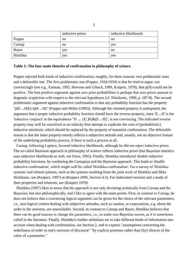
5

inductive priors inductive likelihoods

Popper no no

Carnap no yes

Bayes yes no

Hintikka yes yes

Table 1: The four main theor ies of confirmation in philosophy of science.

Popper rejected both kinds of inductive confirmation, roughly, for three reasons: two problematic onesand a defensible one. The first problematic one (Popper, 1934/1959) is that he tried to argue, notconvincingly (see e.g., Earman, 1992, Howson and Urbach, 1989, Kuipers, 1978), that p(H) could not bepositive. The best positive argument against zero prior probabilities is perhaps that zero priors amount todogmatic scepticism with respect to the relevant hypotheses (cf. Niiniluoto, 1999, p. 187-8). The secondproblematic argument against inductive confirmation is that any probability function has the property

"p(E→H|E)<p(E→H)" (Popper and Miller (1983)). Although the claimed property is undisputed, the

argument that a proper inductive probability function should have the reverse property, since 'E→H' is the

'inductive conjunct' in the equivalence "H ↔ (E∨H)&(E→H)", is not convincing. The indicated reverseproperty may well be conceived as an unlucky first attempt to explicate the core of (probabilistic)inductive intuitions, which should be replaced by the property of instantial confirmation. The defensiblereason is that the latter property merely reflects a subjective attitude and, usually, not an objective featureof the underlying probability process, if there is such a process at all. Carnap, following Laplace, favored inductive likelihoods, although he did not reject inductive priors.The so-called Bayesian approach in philosophy of science reflects inductive priors (but Bayesian statisticsuses inductive likelihoods as well, see Festa, 1993). Finally, Hintikka introduced 'double inductive'probability functions, by combining the Carnapian and the Bayesian approach. This leads to 'doubleinductive confirmation', which might well be called 'Hintikka-confirmation'. For a survey of 'Hintikka-systems' and related systems, such as the systems resulting from the joint work of Hintikka and IlkkaNiiniluoto, see (Kuipers, 1997) or (Kuipers 2000, Section 4.5). For elaborated versions and a study oftheir properties and relations, see (Kuipers 1978). Hintikka (1997) likes to stress that his approach is not only deviating technically from Carnap and theBayesian, but also philosophically, and I like to agree with the main points. First, in contrast to Carnap, hedoes not believe that a convincing logical argument can be given for the choice of the relevant parameters,i.e., non-logical criteria dealing with subjective attitudes, such as caution, or expectations, e.g. about theorder in the universe, are unavoidable. Second, in contrast to Carnap and Bayes, Hintikka believes thatthere can be good reasons to change the parameters, i.e., to make non-Bayesian moves, as it is sometimescalled in the literature. Finally, Hintikka's further ambitions are to take different kinds of information intoaccount when dealing with confirmation, see Section 2, and to express "assumptions concerning theorderliness of order in one's universe of discourse" "by explicit premises rather than [by] choices of thevalue of a parameter."

6

1.2. Degrees of confirmationI now turn to the problem of defining degrees of confirmation, in particular a degree of inductiveconfirmation, even such that it entails a general definition of inductive confirmation. The presentapproach is not in the letter but in the spirit of Mura (1990) (see also e.g., Schlesinger (1995)) and Milne(1996) and Festa (1999). The idea is to specify a measure for the degree of inductive influence bycomparing the relevant 'p-expressions' with the corresponding (structural) 'm-expressions' in anappropriate way. I proceed in three stages.

1.2.1. Stage 1: Degrees of general and structural confirmation

In the first stage I propose, instead of the standard difference measure p(H|E)−p(H), the (non-standardversion of the) ratio measure p(E|H)/p(E) as the degree (or rate) of (backward) confirmation in general(that is, according to some p), indicated by cp(H,E). It amounts to the degree of structural confirmation forp=m. This ratio has the following properties. For p-non-zero hypotheses, it is equal to the standard ratiomeasure p(H|E)/p(H), and hence is symmetric (cp(H,E) = cp(E,H)), but it leaves room for confirmation(amounting to: cp(H,E)>1) of p-zero hypotheses. (For p-zero evidence we might turn to the standard ratiomeasure.) Moreover, it satisfies the comparative principles of deductive (d-)confirmation P1 and P2. Notefirst that cp(H,E) is equal to 1/p(E) when H entails E, for p(E|H)=1 in that case. This immediately impliesP2: if H and H* both entail E then cp(H,E) = cp(H* ,E). Moreover, if H entails E and E* , and E entails E*(and not vice versa) then cp(H,E) > cp(H,E*), as soon as we may even assume that p(E)<p(E*). Thiscondition amounts to (a slightly weakened version of) P1. In agreement with P2 we obtain, for example,that an even outcome with a fair die equally d-confirms the hypotheses { 6} , { 4,6} , and { 2,4,6} , withdegree of (structural and deductive) confirmation 2. This result expresses the fact that the outcomeprobabilities are multiplied by 2, raising them from 1/6 to 1/3, from 1/3 to 2/3, and from 1/2 to 1,respectively. Note also that in the paradigm example of structural non-deductive confirmation, that is, aneven outcome confirms a high outcome, the corresponding degree is (2/3)/(1/2)=4/3. But, in agreementwith P1, the stronger outcome { 4,6} confirms it more, viz., by degree (2/3)/(1/3) = 2. It even verifies thehypothesis. As suggested, there are a number of other degrees of confirmation. Fitelson (1999) evaluates four ofthem, among which the logarithmic forward version of our backward ratio measure, in the light of sevenarguments or conditions of adequacy as they occur in the literature. The ratio measure fails in five cases.Three of them are directly related to the 'pure' character of cp, that is, its satisfaction of P2.1 In Chapter 2of (Kuipers, 2000) P2 is defended extensively. However, I also argue in Chapter 3 of that book, that assoon as one uses the probability calculus, it does not matter very much which 'confirmation language' onechooses, for that calculus provides the crucial means for updating the plausibility of a hypothesis in thelight of evidence. Hence, the only important point, which then remains, is to always make clear which 1 The P2-related arguments concern the first and the second argument in Fitelson's Table 1, and the second in Table 2. Of theother two, the example of 'unintuitive' confirmation is rebutted in (Kuipers, 2000, Chapter 3) with a similar case against thedifference measure. The other one is related to the 'grue-paradox', for which Chapter 2 and 3 of (Kuipers, 2000) claim topresent an illuminating analysis in agreement with P2.

7

confirmation language one has chosen.

1.2.2. Stage 2: The degree of inductive confirmationIn the second stage I define, as announced, the degree of inductive influence in this degree ofconfirmation, or simply the degree of inductive (backward) confirmation (according to p), as the ratio:

rp(H,E) = cp(H,E) = p(E|H)/p(E) cm(H,E) m(E|H)/m(E)

A nice direct consequence of this definition is that the degree of confirmation equals the product of thedegree of structural confirmation and the degree of inductive confirmation. In the following table I summarize the kinds of degrees of confirmation that I have distinguished. For laterpurposes, I also add the log ratio version of the ratio measure and the difference measure and, for enabling easycomparison I mainly list the forward versions of the (log) ratio measures.

A B C D

1 Notion: n(.) ratio doc log ratio doc difference doc

2 degree of confirmation c?p(H;E) cp(H;E) =df

p(E|H)/p(E) =

p(H|E)/p(H) =

p(H&E)/[p(H)p(E)]

clp(H;E) =df

log p(E|H)/p(E) =

log p(H|E)/p(H) =

log p(H|E) − log p(H)

cdp(H;E) =df

p(H|E) − p(H)

3 Relation between prior and

posterior probability and degree

of confirmation

p(H|E) =

p(H) × cp(H;E)

log p(H|E) =

log p(H) + clp(H;E)

p(H|E) =

p(H) + cdp(H;E)

4 degree of structural confirmation

c?m(H;E)

cm(H;E) =df

m(H|E)/m(H)

clm(H;E) =df

log m(H|E)/m(H)

cdm(H;E) =df

m(H|E) − m(H)

5 degree of inductive confirmationr?p(H,E)

[p(H|E)/p(H)] /

[m(H|E)/m(H)]

log [p(H|E)/p(H)] − log [m(H|E)/m(H)]

[p(H|E)−p(H)]− [m(H|E)−m(H)]

TABLE 2: Survey of degrees of confirmation (doc; 'p' fixed)

1.2.3. Stage 3: Four kinds of inductive confirmationIn the third and final stage I generally define inductive confirmation, that is, E inductively confirms H, ofcourse, by the condition: rp(H,E) > 1. This definition leads to four interesting possibilities forconfirmation according to p. Assume that cp(H,E) > 1, that is, assume E confirms H according to p. The first possibility is purelystructural confirmation, that is, rp(H,E) = 1, in which case the confirmation has no inductive features. Thistrivially holds in general for structural confirmation, but it may occasionally apply to cases ofconfirmation according to some p different from m. The second possibility is that of purely inductiveconfirmation, that is, cm(H,E) = 1, and hence rp(H,E) = cp(H,E). This condition typically applies in thecase of (purely) instantial confirmation, since, e.g., m(Fa|Fb&E)/m(Fa|E)=1. The third possibility is that of a combination of structural and inductive confirmation: cm(H,E) and

8

cp(H,E) both exceed 1, but the second more than the first. This type of combined confirmation typicallyoccurs when a Carnapian inductive probability function is assigned, e.g., in the case of a die-like object ofwhich it may not be assumed that it is fair. Starting from equal prior probabilities for the six sides, such afunction gradually approaches the observed relative frequencies. If among the even outcomes a highoutcome has been observed more often than expected on the basis of equal probability then (only)knowing in addition that the next throw has resulted in an even outcome confirms the hypothesis that it isa high outcome in two ways: structurally (as I showed already in 1.2.1) and inductively.

Let n be the total number of throws so far, let ni indicate the number of throws that have resultedin outcome i (1,...,6). Then the Carnapian probability that the next throw results in i is

(ni+λ/6)/(n+λ), for some fixed finite positive value of the parameter λ. Hence, the probability that

the next throw results in an even outcome is (n2+n4+n6+λ/2)/(n+λ), and the probability that it is

'even-and-high' is (n4+n6+λ/3)/(n+λ). The ratio of the latter to the former is the posteriorprobability of a high next outcome given that it is even and given the previous outcomes. It is noweasy to check that in order to get a degree of confirmation larger than the structural degree, whichis 4/3 as I have noted before, this posterior probability should be larger than the correspondinglogical probability, which is 2/3. This is the case as soon as 2n2 < n4+n6, that is, when the averageoccurrence of '4' and '6' exceeds that of '2'.

It is easy to check that the same example when treated by a Hintikka-system (for references, seeSubsection 1.1.2.2.) shows essentially the same combined type of structural and inductive confirmation. Let me finally turn to the fourth and perhaps most surprising possibility: confirmation combined withthe 'opposite' of inductive confirmation, that is, rp(H,E) < 1, to be called counter-inductive confirmation.Typical examples arise in the case of deductive confirmation. In this case rp(H,E) reduces to m(E)/p(E),which may well be smaller than 1. A specific example is the following: let E be Fa&Fb and let p beinductive then E d-confirms "for all x Fx" in a counter-inductive way. On second thought, the possibilityof, in particular, deductive counter-inductive confirmation should not be surprising. Inductive probabilityfunctions borrow, as it were, the possibility of inductive confirmation by reducing the available 'amount'of possible deductive confirmation. To be precise, deductive confirmation by some E is counter-inductiveas soon as E gets 'inductive load' (see Subsection 3.1) from p, i.e., m(E)<p(E). The following table summarizes the distinguished kinds of confirmation: general and deductive.

9

A: kind B: condition C: degree of confirmation =

General confirmation cp(H,E) >1

1 Purely inductive confirmation:

e.g. instantial confirmation

cp(H,E)>cm(H,E)=1 degree of inductive confirmation

2 Combined ( inductive and

structural) confirmation:

cp(H,E)>cm(H,E)>1 degree of structural confirmation

× degree of inductive confirmation

3 Purely structural confirmation: cp(H,E)=cm(H,E)>1 degree of structural confirmation

4 Counter-inductive confirmation: cm(H,E)>cp(H,E)>1 degree of structural confirmation

× degree of "inductive" confirmation

Deductive confirmation H |= E, and hence

p(E|H)=m(E|H)=1

cp(H,E)= 1/ p(E) = [1/m(E)] (m(E)/p(E)) =

cm(H,E) rp(H,E)

5 Purely inductive confirmation impossible, if m(E)<1

6 Combined (inductive and structural)

confirmation

m(E) > p(E)

7 Purely structural confirmation m(E) =p(E)

8 Counter-inductive confirmation m(E) < p(E)

TABLE 3: Survey of kinds of inductive confirmation in terms of ratio degrees of confirmation ('p'fixed, 'm': logical measure function)

2. Kinds of information and their relevance for explanation and generalization

Drawing upon the work of Carnap, Bar-Hillel, Popper, Törnebohm and Adams, Hintikka (1968) hasintroduced in a systematic way two kinds of information, indicated as surprise value and substantiveinformation, and briefly called information and content. When representing them I will point out the closerelation between transmitted information and transmitted content on the one hand and certain degrees of

confirmation on the other. Moreover, I will characterize Hintikka's aims and claims regarding the choicebetween hypotheses when dealing with explanation and generalization in relation to (transmitted)information and content. All references are to (Hintikka, 1968), except when otherwise stated.

2.1. Kinds of information2.1.1. Surprise value information

The first kind of information is related to the surprise value or unexpectedness of a statement. As now isusual in computer science, Hintikka focuses on the logarithmic versions of the relevant notions for theirnice additive properties. However, as in the case of confirmation, I prefer and start each time with thenon-logarithmic versions for their conceptual simplicity. I begin with the prior (or absolute), the posterior(or posterior or conditional) and the transmitted notions of information.

The prior information contained in a statement, e.g. a hypothesis H, is supposed to be inversely related toits probability in the following way:

10

i(H)=df 1/p(H)

inf (H)=df log i(H) = log 1/p(H) = −log p(H)

The posterior version aims to capture how much information this hypothesis, ‘adds to’ or ‘exceeds’another, e.g. an evidential statement E, assuming E:

i(H|E)=df 1/p(H|E) = p(E)/p(H&E) = i(H&E)/i(E)

inf (H|E)2 =df − log p(H|E) = log i(H|E) = inf(H&E)−inf(E)

Hintikka calls the inf(H|E) the incremental or conditional information. Now I turn to the idea ofinformation transmission: how much information does E 'convey concerning the subject matter' of H, ortransmit to H, assuming E:

trans-i(E;H)=df i(H|E)/i(H) = p(H|E)/p(H)

trans-inf(E;H)3=df inf(H)−inf(H|E) = log trans-i(H;E) = log p(H|E) − log p(H)

According to Hintikka, we may say that trans-inf(E;H) (and hence trans-i(E;H)) “measures the reductionof our uncertainty concerning H which takes place when we come to know, not H, but E” (p. 316, where Ihave replaced the relevant symbols). It is directly clear that trans-i(E;H) coincides with the forward ratio measure of confirmation cp(H;E),and hence that it is symmetric, that is, it equals trans-i(H;E) when p(E) and p(H) are non-zero. However, ifp(H) is 0 and p(E) non-zero, trans-i(E;H) is undefined (hence, it may be equated with 1), but trans-i(H;E)may well be defined, viz. when p(E|H) is defined. For instance, in case H entails E trans-i(H;E) = 1/p(E),that is, H reduces the uncertainty regarding E from 1/p(E) to 1 (certainty). Trans-inf(E;H) coincides ofcourse with the logarithmic version of the ratio measure, viz. clp(H;E), and similar remarks apply.

2.1.2. Substantive information

The second kind of information is related to the content or substantive information contained in astatement. Now there are no relevant logarithmic versions. Again I define the prior, the posterior (orconditional) and the transmitted notions of substantive information.

The prior content of a statement, e.g. a hypothesis H, is made inversely related to its probability byequating it with the probability of its negation:

2 Here I start to deviate somewhat from Hintikka's notation. Hintikka's "infadd(H|E)", (4), p. 313, and "infcond(H|E)", (9), p. 315,both correspond with "inf(H|E)", as he notes on p. 315 on the basis of (6) on p. 314.3 "trans-inf(E;H)" corresponds with Hintikka's notion (11) on p. 316, indicated by him as "transinf(E|H)" on p. 317.

11

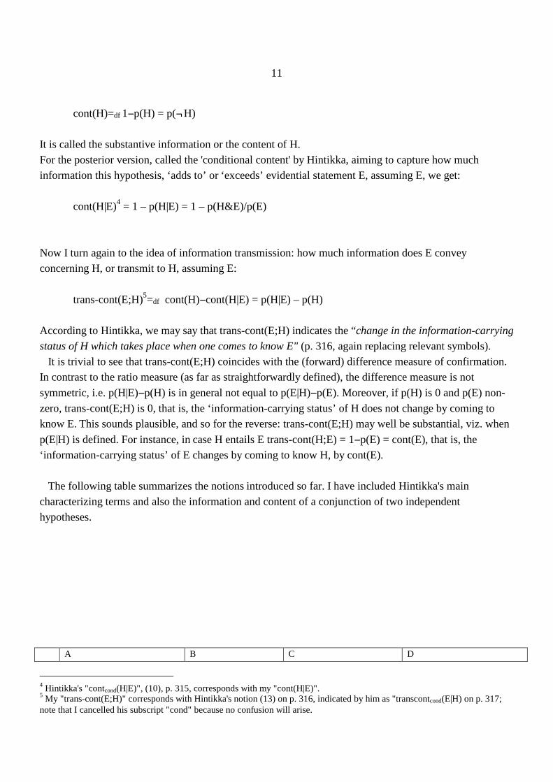
cont(H)=df 1−p(H) = p(¬H)

It is called the substantive information or the content of H.For the posterior version, called the 'conditional content' by Hintikka, aiming to capture how muchinformation this hypothesis, ‘adds to’ or ‘exceeds’ evidential statement E, assuming E, we get:

cont(H|E)4 = 1 – p(H|E) = 1 – p(H&E)/p(E)

Now I turn again to the idea of information transmission: how much information does E conveyconcerning H, or transmit to H, assuming E:

trans-cont(E;H)5=df cont(H)−cont(H|E) = p(H|E) – p(H)

According to Hintikka, we may say that trans-cont(E;H) indicates the “change in the information-carrying

status of H which takes place when one comes to know E" (p. 316, again replacing relevant symbols). It is trivial to see that trans-cont(E;H) coincides with the (forward) difference measure of confirmation.In contrast to the ratio measure (as far as straightforwardly defined), the difference measure is not

symmetric, i.e. p(H|E)−p(H) is in general not equal to p(E|H)−p(E). Moreover, if p(H) is 0 and p(E) non-zero, trans-cont(E;H) is 0, that is, the ‘ information-carrying status’ of H does not change by coming toknow E. This sounds plausible, and so for the reverse: trans-cont(E;H) may well be substantial, viz. when

p(E|H) is defined. For instance, in case H entails E trans-cont(H;E) = 1−p(E) = cont(E), that is, the‘ information-carrying status’ of E changes by coming to know H, by cont(E).

The following table summarizes the notions introduced so far. I have included Hintikka's maincharacterizing terms and also the information and content of a conjunction of two independenthypotheses.

A B C D

4 Hintikka's "contcond(H|E)", (10), p. 315, corresponds with my "cont(H|E)".5 My "trans-cont(E;H)" corresponds with Hintikka's notion (13) on p. 316, indicated by him as "transcontcond(E|H) on p. 317;note that I cancelled his subscript "cond" because no confusion will arise.

12

1 Notion: n(.) Information: i(.) log-information: inf(.) content: cont(.)

2 Prior value: n(H) i(H)=df 1/p(H) inf(H)=df − log p(H) cont(H)=df 1−p(H)

Hintikka the surprise value or

unexpectedness of (the truth

of) H

the substantive information or

content of H

3 n(H&H') for independent Hand H', hence, p(H&H')=p(H)

× p(H')

i(H)×i(H') inf(H)+inf(H') cont(H&H')=

cont(H) + cont(H') −cont(H)×cont(H')

4 Posterior value of H given E:

n(H|E)

i(H|E)=df

1/p(H|E) = i(H&E)/i(E)

inf(H|E) =df

−log p(H|E) =

inf(H&E) − inf(E)

cont (H|E) =df

1 − p(H/E) =

1− p(H&E)/p(E)

Hintikka incremental information

(conditional information)

conditional content

5 Transmitted value (from E to

H): trans-n(E;H)

corresponds to doc

trans-i(E;H) =df

i(H)/i(H|E) =

p(H|E)/p(H) = cp(H;E)

trans-inf(E;H) =df

inf(H) − inf(H|E) =

log p(H|E) − log p(H) =

clp(H;E)

trans-cont(E;H) =df

cont(H) − cont(H|E) =

p(H|E) − p(H) =

cdp(H;E)

Hintikka the information E conveys

concerning the subject

matter of H

the change in the content of H

due to E

Transmitted value =df prior value / (resp. −) posterior value =

(log) posterior probability / (resp. −) (log) prior probability =df degree of confirmation

TABLE 4: Survey of definitions of ' information' and 'content' ('p' fixed)

In the last row I have also included a compact indication of the plausible relations between the variousnotions. For the non-logarithmic version of information we get more specifically:

transmitted value =df prior value /posterior value =posterior probability /prior probability =df (forward) ratio degree of confirmation

For the logarithmic version of information we get:

transmitted value =df prior value − posterior value =

log posterior probability − log prior probability =df log ratio degree of confirmation

Finally for the notion of content we get:

transmitted value =df prior value − posterior value =

posterior probability − prior probability =df difference degree of confirmation

13

Let me illustrate the different notions by the fair die (recall, E/H: even/high outcome), where p=m. For thei-notions we get i(E)=i(H)=2, i(H|E)=i(E|H)=3/2, cm(H;E) = trans-i(E;H) = (2/3)/(1/2)=4/3. For the inf-notions we simply get the logarithms of these values. For the cont-notions we get: cont(E)=cont(H)=1/2,cont(H|E)=cont(E|H)=1/3, cdp(H;E) = trans-cont(E;H) = 2/3-1/2=1/6.

2.1.3. Implication related notionsStrangely enough, Hintikka introduces as a variant of 'conditional content' cont(H|E) an alternativedefinition, called 'incremental content', where E is not assumed as 'posterior' condition, but only figuring

as condition in the implication E→H, viz.

cont→(H|E)6 = cont (E→H) = 1 – p(E→H)

Although Hintikka introduces a separate notation for "cont(E→H)", I am puzzled why he does not even

mention its formal analogue "inf(E→H)", let alone "i (E→H)":

i→(H|E) =df i (E→H) = 1/p(E→H)

and its (logarithmic) inf-version

inf→(H|E) =df inf (E→H) = − log p(E→H)

It is unclear why Hintikka compared, in fact, the pair "inf(H|E)" and "cont(E→H)", even two times (viz.,

(4) and (5), (6) and (7), respectively). The plausible comparisons seem to be both the pair "inf(E→H)" and

"cont(E→H)" and the pair "inf(H|E)" and "cont(H|E)". He only compares the last pair (by (9) and (10)).The only reason for the first mentioned comparison seems to be the 'additive' character of both itsmembers (as expressed by (4) and (5)).

For later purposes I introduce Hintikka's definition of the corresponding transmission concept ofincremental content.

trans-cont→(E;H)7 =df cont(H) − cont→(H|E) = cont(H) − cont(E→H) = 1 − p(HvE)

Similarly we can define:

6 Hintikka's "contadd(H|E)", (5), p. 313, corresponds with "cont(E→H)", and hence with my cont→(H|E), as he notes by (7) on p.314.

7 "trans-cont→(E;H)" corresponds with Hintikka's notion (12) on p. 316., indicated by him as "transcontadd(E|H) on p. 317.

14

trans-inf→(E;H) =df inf(H) − inf(E→H) = log p(E→H)/p(H)

and hence

trans-i→(E;H) =df i(H)/i(E→H) = p(E→H)/p(H)

The following survey can now be made:

A B C D

1 Notion: n(.) information: i(.) log-information: inf(.) content: cont(.)

2 Prior value: n(H) i(H)=df 1/p(H) inf(H)=df − log p(H) cont(H)=df 1−p(H)

Hintikka the surprise value or

unexpectedness of (the

truth of) H

the substantive information or

content of H

3 Value of implication:

(E→H)

i→(H;E)=df i(E→H) =

1/p(E→H)

inf→(H;E)=df inf(E→H) =

− log p(E→H)

cont→(H;E) =df cont(E→H) =

1−p(E→H) = cont(H&E) −cont(E)

Hintikka incremental content

4 "Transmitted value by

→" (from E to H by

E→H): trans-n→(E;H)

trans-i→(E;H) =df

i(H)/i(E→H)

trans-inf→(E;H) =df

inf(H) − inf(E→H) =

log p(E→H)/p(H)

trans-cont→(E;H) =df

cont(H) − cont→(H|E) =

cont(H) − cont(E→H) =

1 − p(HvE)

Hintikka the information E conveys

concerning the subject matter

of H

TABLE 5: Definitions of ' information' and 'content' related to the implication ('p' fixed)

2.2. Explanation and generalizationFrom Section 7 on, it becomes clear where Hintikka is basically aiming at with his distinction betweeninformation and content. According to him there is a strong relation with different targets of scientificresearch. Let me quote him extensively in this matter:

" ……. One of the most important uses that our distinctions have is to show that there are several different

ways of looking at the relation of observational data to those hypotheses which are based on them and

which perhaps are designed to explain them. In different situations the concept of information can be

brought to bear on this relation in entirely different ways. …… ……………… In general, the scientific

search for truth is much less of a single-goal enterprise than philosophers usually realize, and suitable

distinctions between different senses of information perhaps serve to bring out some of the relevant

differences between different goals.

Let us consider some differences between different cases. One of the most important distinctions here is

15

between, on one hand, a case in which we are predominantly interested in a particular body of

observations E which we want to explain by means of a suitable hypothesis H, and on the other hand a

case in which we have no particular interest in our evidence E but rather want to use it as a stepping-stone

to some general theory H which is designed to apply to other matters, too, besides E. We might label these

two situations as cases of local and global theorizing, respectively. Often the difference in question can

also be characterized as a difference between explanation and generalization, respectively. Perhaps we can

even partly characterize the difference between the activities of (local) explanation and (global) theorizing

by spelling out (as we shall proceed to do) the differences between the two types of cases." (Hintikka,

1968, p. 321, symbols adapted, TK)

"It is important to realize, however, that in this respect [explanation versus generalizing, TK] the interests

of a historian are apt to differ from those of a scientist." (ibid. p. 324).

Hintikka argues at length in Section 8 that in the case we want to explain some evidence E by ahypothesis, we have good reasons, in his own words, replacing symbols: "to choose the explanatoryhypothesis H such that it is maximally informative concerning the subject matter with which E deals.Since we know the truth of E already, we are not interested in the substantive information that H carriesconcerning the truth of E. What we want to do is to find H such that the truth of E is not unexpected,given H." (p. 321). This brings him immediately to a plea for maximizing the transmitted informationtrans-inf(E;H), which was seen to be equal to log p(E|H)/p(E). For fixed E, this amounts of course tosupport of the so-called maximum likelihood principle in this type of case: choose H such that p(E|H) ismaximal. For global theorizing or generalization Hintikka argues extensively in Section 9 that we shouldconcentrate on maximizing relevant content notions. As a matter of fact, he has four arguments in favor ofthe claim that we should choose that hypothesis that maximizes the transmitted content, given E, that is,

p(H|E) − p(H). Strangely enough, he only hints upon the only direct argument for this by speaking of "thefourth time" that this expression is to be maximized, whereas he only specifies three, indirect, arguments.However, it is clear that maximizing the transmitted content is an argument in itself, not in the least,because it amounts to maximizing the difference degree of confirmation. But his three indirect argumentsare more surprising, or at least two of them. These three arguments are all dealing with notions of 'expected value gains' 8. First he notes that the'(posterior) expected content gain', plausibly defined by

p(H|E)× cont(H) − p(¬H|E)× cont(¬H)

is maximal when p(H|E) − p(E) is maximal. Then he argues that the 'expected transmitted content gain',similarly defined by

8 In Section 6 Hintikka writes down the (posterior) expected transmitted values for trans-inf(E;H), trans-cont(E;H) and trans-cont→(E;H) and it would be easy to add those for trans-i(E;H), trans-i→(E;H) trans-inf→(E;H). However, as we will see in thetext some of the so-called 'expected value gains' are much more interesting.

16

p(H|E)× trans-cont(E;H) − p(¬H|E)× trans-cont(E;¬H)

is also maximized by the same condition. The latter does not need to surprise us very much because the

'expected posterior value gain', viz. p(H|E)×cont(H|E) − p(¬H|E)×cont(¬H|E), is easily seen to be 0,whereas cont(H)=trans-cont(E;H) + cont (H|E).

The third indirect argument is again surprising. It turns out that maximizing p(H|E) − p(E) also leads tomaximizing the 'expected transmitted incremental content gain', that is:

P(H|E)×trans-cont→(E;H) − p(¬H|E)×trans-cont→(E;¬H)

In sum, in the context of generalization, Hintikka has impressive 'expectation' arguments in favor ofmaximizing the transmitted content. However, I have nevertheless strong doubts about his considerations. Hintikka’s plea for maximizationof the transmitted content and hence of the difference degree of confirmation has strange consequences.Consider the case that hypotheses H and H* have equal likelihood in view of E. Suppose, morespecifically, that H and H* entail E, and hence that p(E|H) = p(E|H*) =1. Then it is easy to check that

maximization of p(H|E) − p(H) = p(H)(p(E|H)/p(E) − 1) leads to favoring the more probable hypothesisamong H and H*. This is a direct illustration of the fact that the difference measure does not satisfy P.2,see Subsection 1.1.1.. Its 'impure' character9 in the form of the Matthew-effect, the more probablehypothesis is rewarded more for the same success, is, surprisingly enough, shared by Popper’s favoritemeasures of corroboration (see Kuipers 2000, Appendix 1 of Ch. 3). If any preference is to be expected Iwould be more inclined to think of the reverse preference in the 'context of generalization': if twohypotheses are equally successful with regard to the evidence, then the stronger hypothesis seems morechallenging to proceed with. Apart from the fact that Popper would not appreciate the notion of'generalization', this would be very much in Popperian spirit. On the other hand, in the 'context ofexplanation' one might expect a preference for the weaker hypothesis: if one wants to explain somethingon the basis of the available knowledge one will prefer, among equally successful hypotheses regardingthe evidence, the hypothesis that has the highest initial probability, that is, to be precise, the highestupdated probability just before the evidence to be explained came available. However, this is not intendedto reverse Hintikka's plea into a plea for maximizing likelihood in the case of generalization, for thiswould, of course, not work in the case of equal likelihoods. But a partial criterion would be possible:when the likelihoods are the same, such as is the case for deductive confirmation, favor the weakerhypothesis for explanation purposes and the stronger for generalization purposes10. However, even this

9 Comparing the 'impure' degree p(H|E)-p(H)= p(H)(p(E|H)/p(E) − 1) with the 'pure' degree p(E|H)/p(E) makes clear that p(H)can even be considered as a measure of the impurity in the former, at least when the likelihoods are the same.10 Another option would be to maximize the 'expected i-gain’ , the analogue of expected content gain, which equals

p(H|E)/p(H) − p(¬H|E)/p(¬H) = p(E|H)/p(E) − p(E|¬H)/p(E), which leads to favoring the one with the lowest likelihood of

the negation, also called the degree of disconfirmation. This sounds plausible: when the degree of confirmation does not

discriminate, prefer the hypothesis with the lowest degree of disconfirmation. However, it remains unclear whether this option

is more appropriate for explanation rather than for generalization.

17

partial criterion can be questioned because the choice still depends very much on the used probabilityfunction. Moreover, it is not easy to see how to proceed in the case of different likelihoods. Simplymaximizing likelihood then would discard probability considerations that seem at least to be relevantwhen the likelihoods do not discriminate. In the next section I will start to elaborate an alternative view on explanation and generalization, bytaking structural and inductive aspects into account. I conclude this section with a totally different criticalconsideration regarding the notion of 'transmitted content'. One attractive aspect of the notion of content,whether prior or posterior, is that it has a straightforward qualitative interpretation. If Struct(L) indicatesthe set of structures of language L and Mod(H) the set of models on which H is true, than the latter's

complement Struct(L)−Mod(H) not only represents Mod(¬H) but is also, as Hintikka is well aware,precisely the model theoretic interpretation of Popper's notion of empirical content of H. Hence, cont (H)=

p(¬H) may be reconstrued as the p(Mod(¬H) )/p(Struct(L)), where the p(Struct(L)=1. Similarly,

cont(H|E) may be seen as the probabilistic version of the posterior empirical content of H, viz. Mod(E) −Mod (H). However, I did not succeed in finding a plausible qualitative interpretation of Hintikka's notionof transmitted content. If such an interpretation cannot be given, it raises the question whether 'transmittedcontent' is more than a somewhat arbitrary notion. Note that a similar objection would apply to the notionof 'transmitted information' if it would turn out not to be possible to give an interpretation of it in terms of(qualitative) bits of information, of which it is well known that it can be given for the underlying notionsof prior and posterior information, assuming that 2 is used as the base of the logarithm.

3. Structural and inductive aspects of explanation and generalization

Whereas Hintikka tries to drive a wedge between explanation and generalization by the distinctionbetween (logarithmic) information and content, in particular the transmitted values, I would like tosuggest that the distinction between structural and inductive aspects of these and other notions are at leastas important. Hence, first I will disentangle these aspects for some crucial notions in a similar way as I didfor confirmation. Next, I will discuss what to maximize in the service of explanation and generalization.Since there do not seem to be in the present context (extra) advantages of the logarithmic version of'surprise value' information, I will only deal with the non-logarithmic version, from which the logarithmicversion can easily be obtained if one so wishes.

3.1. Structural and inductive aspects of probability and types of informationAs we have seen in Subsection 1.2 confirmation has structural and inductive aspects, resulting from acomparison of the values belonging to one's favorite p-function, with the corresponding structural values,that is, the values belonging to the logical measure (m-) function. I will extend this analysis to prior andposterior probabilities and to transmitted information and content. From now on I will call the p-functionthe 'subjective' probability function. However, I hasten to say that 'subjective' is not supposed to mean

18

'merely subjective', because such a function may well have been designed in a rather rational way, asCarnap and Hintikka have demonstrated very convincingly. Let me start by defining the 'inductive load' of prior and posterior subjective probability and of the 'extrainductive load' of the latter relative to the former. There are of course two versions: a ratio and adifference version. In the following table I have depicted all of them.

A B: ratio loads C difference loads

1 Prior inductive load: ni(H) p(H)/m(H) p(H)−m(H)

2 Posterior inductive load:

nI(H|E)

p(H|E)/m(H|E) p(H/E) − m(H|E)

3 Extra inductive load of

posterior probability =

Degree of inductive

confirmation c?p(H;E) =

Inductive load in

transmitted i/ cont

[p(H|E)/m(H|E]

/[p(H)/m(H)]

= [p(H|E)/p(H)] /

[m(H|E)/m(H)]

[p(H|E)−m(H|E)] −[p(H)−m(H)]

= [p(H|E)−p(H)]− [m(H|E)−m(H)]

TABLE 6: (Extra) inductive loads in probabilities ('p' fixed, 'm': logical measure function)

It is easy to check that the extra inductive load of the posterior probability relative to the prior probability,as indicated in Row 3, is equal to the relevant degree of inductive confirmation as defined in Subsection1.2. However, the latter degrees also equal the ratio or the difference of the transmitted type ofinformation to the corresponding transmitted type of structural information. Hence, it is plausible todefine them also as the 'inductive load' of the transmitted type of information. Accordingly, for the ratioversions of loads and degrees we get the conceptual relations:

extra inductive (ratio) load (of posterior probability to the prior)=df posterior inductive load /prior inductive load= degree of subjective confirmation /degree of structural confirmation=df degree of inductive confirmation= transmitted subjective information / transmitted structural information=df inductive load of transmitted information

And for the difference versions:

extra inductive (difference) load (of posterior probability to the prior)

=df posterior inductive load − prior inductive load

= degree of confirmation − degree of structural confirmation=df degree of inductive confirmation

= transmitted subjective content − transmitted structural content=df inductive load of transmitted content

19

Turning to the question of how to define the (extra) inductive loads of prior and posterior information andcontent, it is not immediately clear how to proceed. For example, in the difference version it was rather

plausible to define the inductive load of the prior subjective probability by p(H)−m(H). In view of the

definition of content, 1 − p(H), it now seems plausible to define the inductive load in the prior content by

[1−p(H)]−[1−m(H)] = m(H)−p(H), and hence equal to 'minus the inductive load' in the prior subjectiveprobability. However, one might also argue for equating the inductive (difference) loads of probability

and content, or one might define the inductive load as the absolute value |p(H) − m(H)|. Similarconsiderations and possibilities apply to the ratio versions. However, it is not clear whether we really needall these definitions. Let us see how far we can come by restricting inductive aspects to the probabilitiesconstituting information and content and to the 'corresponding' degrees of confirmation, and hence to thetransmitted types of information.

3.2 Explanation and generalization reconsideredIn Subsection 2.2, I discussed Hintikka's arguments in favor of maximizing transmitted information, andhence the (log) ratio degree of confirmation and even the likelihood, for explanation purposes andmaximizing the transmitted content, and hence the difference degree of confirmation, for generalizationpurposes. It turned out that these preferences have strange consequences, in particular in the case of equallikelihoods, notably deductive confirmation. Moreover, Hintikka's perspective seemed rather restricted bytaking only one probability function into account. In my opinion at least the subjective and the structuralprobability function should be taken into account. My claim in this subsection will be that the structuraland inductive aspects may be particularly relevant when we want to compare appropriate explanation andgeneralization strategies. Roughly speaking, I will suggest that inductive features should be minimized inthe case of explanation in favor of structural features, and the reverse in the case of generalization. Our leading question is: What do we want to maximize or minimize in choosing a hypothesis, given thestructural m-function and a fixed subjective p-function, when explaining E, and when generalizing fromE, respectively? I will certainly not arrive at final answers, but only make a start with answering thesequestions.11 The basic candidate values for comparison seem to be the prior and posterior probabilitiesand the degree of confirmation or, equivalently, the transmitted type of information. In all cases we cancompare subjective, structural and inductive values and in the case of inductive loads and degrees ofconfirmation we can choose at least between ratio and difference measures. Regarding information andcontent we should keep in mind that maximizing probabilities amounts to minimizing both of them. In thefollowing table I have depicted the basic candidate values for maximization or minimization, andindicated Hintikka's preferences for explanation and generalization (indicated in cells 9F and 12F, resp.)and my tentative partial answers (1F and 2F, respectively), which are strongly qualified in the text.

11 Moreover, I will neglect the possibility of combining the perspectives of explanation and generalization. This might be donein similar ways as truth-value and informativeness have been combined by Isaac Levi for epistemic utility and Ilkka Niiniluotofor truthlikeness (see Niiniluoto, 1999, p. 168-170). I thank Allard Tamminga for drawing my attention to this type ofpossibility.

20

A B C D E F

1 structural m(H) TK: maximize for

deductive explanation

2 subjective p(H) TK: maximize for

inductive generalization

3 ratio p(H)/m(H)

4

prior

probability

inductive

load difference p(H)−m(H)

5 structural m(H|E)

6 subjective p(H|E)

7 ratio p(H|E)/m(H|E)

8

posterior

probability Inductive

load difference p(H|E)−m(H|E)

9 ratio = transmitted structural

information

m(H|E)/m(H)

10

structural

difference = transmitted structural

content

m(H|E)−m(H)

11 ratio = transmitted subjective

information

p(H|E)/p(H) JH: maximize when

explaining

12

subjective

difference = transmitted subjective

content

p(H|E)−p(H) JH: maximize when

generalizing

13 ratio = extra inductive (ratio)

load of posterior

probability =

inductive load of

transmitted information

[p(H|E)/m(H|E]

/[p(H)/m(H)] =

[p(H|E)/p(H)/

[m(H|E)/m(H)]

14

degree

of

confirmationinductive

difference = extra inductive (diff.)

load of posterior

probability =

inductive load of

transmitted content

[p(H|E)−m(H|E)] −[p(H)−m(H)] =

[p(H|E) − p(H)] −[m(H|E) − m(H)]

Table 7: Possibilities for maximizing or minimizing when choosing H, for given p and m (p/m:subjective/structural probability)

Our start will be restricted to the case of equal likelihoods, more specifically, deductive confirmation,and is particularly intended to invite Hintikka to develop his intuitions regarding inductive aspects further.When H and H* both entail E, all relevant likelihoods are simply 1. Hence, maximizing whateverlikelihood will then not work. Moreover, as I have pointed out in Subsection 1.2, see Table 3, deductiveconfirmation based on p will be counter-inductive as soon as p(E) has inductive load in the sense ofexceeding m(E). We have also seen, in Subsection 2.2, that maximizing the transmitted subjectivecontent, as Hintikka proposed for generalizing, would favor, quite counterintuitively, the weakerhypothesis.12 But for explanation purposes this might not be so counter-intuitive. 12 Note that when one hypothesis is stronger than the other due to logically entailing the other, comparing m-values will lead tothis same conclusion as comparing p-values.

21

So let us first concentrate on explanation. When we merely want to (deductively) explain a certainphenomenon on the basis of the available knowledge, including hypotheses with various probabilities, wewould like to be safe. However, instead of saying that this is based on the difference measure ofconfirmation, I rather prefer to see the preference as essentially based on the following sextuple: <p(H),p(E), p(E|H), m(H), m(E), m(E|H)>, in terms of which the other notions can be defined. Hence, mytentative answer is that in the context of deductive explanation in the face of deductive confirmation, ormore generally in the case of equal likelihoods, the more probable hypothesis should be preferred. This isa robust strategy as far as the comparisons of p- and m-values coincide, or are at least not opposite, whichwill at least automatically be the case when one of the hypotheses entails the other. However, at least thefollowing interesting questions then remain.

(1) What to do when the comparison of m-values diverges from that of p-values?I will deal separately with an extreme and a special case, respectively:

(2) What to do when p(H)=p(H*)=1 and hence when both are considered to be establishedbackground knowledge, and hence when we will also have m(H)=m(H*)=1?(3) What to do when the m-values of both hypotheses are 0 and the p-values non-zero?

Regarding the first case, I would like to suggest that the hypothesis with the highest prior m-value is themost plausible one to choose. The reason is that the higher subjective prior probability is apparently notdue to logico-structural considerations but to inductive considerations of one kind or another, e.g. order(simplicity, homogeneity) or analogy influences. In the second case, the proper conclusion is that there isapparently more than one valid explanation available. In the third case, and more generally when the priorm-values do not differ, our preferences may well depend on the reason why one subjective priorprobability exceeds another. This may be due to the fact that one hypothesis is weaker than the other insome logico-structural sense, which cannot be accounted for by the m-function; this may well be the casefor m-zero hypotheses. E.g. "All A and B are F" and "All C are F" may both get m-value 0, but the firstclaims in a sense more than the second. In such a case, preferring the one with the higher p-value, due tothis aspect, seems plausible for explanation purposes. However, the higher p-value may also be (mainly)due to typical inductive considerations, whereas the relevant hypotheses are logico-structurallycomparable. E.g. the one may have more analogical features than the other, accounted for by a higherprior subjective probability. In such a case it will be difficult to choose. However, if the other hypothesisis logico-structurally weaker, but not accounted for by 0 m-values, that one seems preferable again. Similarly interesting questions remain when I turn to the suggested answer in the case of generalizing:in the context of (inductive) generalization13 from E by hypotheses that are deductively confirmed by E,the less probable hypothesis should prima facie be preferred. However, before I discuss these questions, Ihave to address the so-called 'converse consequence property' of deductive confirmation of H by E, that is,the fact that of any stronger hypothesis than H is also deductively confirmed by E, including any oneresulting from conjugating H with a totally unrelated additional hypothesis. Of course, we should notprefer such a type of stronger hypothesis. As I have argued (Kuipers, 2000, 2.1.2), in such a case theconfirmation remains perfectly localizable. Hence, in this case we should only compare hypotheses that 13 Note that using here the phrase 'deductive generalization' would be highly misleading, but 'inductive generalization' isappropriate, in particular as far as generalizations are concerned that are formulated in the same language as the evidence.

22

are relevant in a sense to be specified, where our limited knowledge of deductive relations should ideallyalso be taken into account. Assuming that such a definition can be given, the suggestion is that the lessprobable of the relevant hypotheses should be preferred. Preference here of course means preference forfurther testing and evaluation, not yet for acceptance, even if that is only for the time being. Let me now turn to the three remaining questions or cases applied to relevant hypotheses in the contextof generalization. Regarding (1), what to do when the p-comparison differs from the m-comparison, Iwould now like to suggest that the hypothesis with the lowest prior p-value is the most plausible one tochoose. The reason is the mirror image of the one in the case of explanation. The lower subjective priorprobability is apparently not due to logico-structural considerations but to inductive considerations infavor of other hypotheses; after all, assigning higher probabilities to some hypotheses on the basis of orderor analogy considerations has to be paid by other hypotheses. In case (2), the 'hypotheses' in question willnot be considered as interesting new generalizations because they belong already to the backgroundknowledge. In case (3), when both prior m-values are 0, and more generally when the prior m-values donot differ, our preferences will again depend on the reason why one subjective prior probability exceedsanother. It may be due to the fact that the one hypothesis is weaker in some logico-structural sense, whichcannot be accounted for by the m-function. In such a case, focussing on the one with the lower p-value,due to this way of being stronger, seems plausible for generalization purposes. However, the lower p-value may also be (mainly) due to typical inductive considerations, working positive for other hypotheses.If another hypothesis is logico-structurally stronger, but which is not accounted for by 0 m-values, thatone seems now preferable to proceed with. In sum, as far as choosing between different deductive explanations of new evidence is concerned, mypreference goes in the direction of higher structural prior probabilities, with a number of qualifications.On the other hand, as far as choosing between different inductive generalizations is concerned, mypreference goes in the direction of lower subjective prior probabilities, with even more qualifications. Inboth cases the relevant degrees of confirmation and hence the transmitted information do not differ, forthe corresponding likelihoods do not differ. I leave the question of how to deal with cases of differentlikelihoods open.

Concluding remarks

From Section 2 and 3 it is rather clear that we are far from a final answer to the question how to useprobabilities, and measures of confirmation, information and content in the contexts of explanation andgeneralization. However, I hope to have convinced the reader, and in particular Jaakko Hintikka, whateverthe role of different kinds of information, structural and inductive aspects should also play a role. Iconclude this paper by enlarging the problem of choices to be made. It is surprising that Hintikka did not explicitly consider the information-theoretic notion of entropy,although he took the corresponding logarithmic notion of information extensively into account. Entropynot only naturally leads to new preference criteria between different hypotheses, but it also suggestspreference criteria between different probability functions for the same set of (mutually exclusive and

23

together exhaustive) hypotheses. Let me start with the first. The prior entropy is defined as the prior expected prior (logarithmic)information:

−p(H)log p(H) − p(¬H)log p(¬H)

Similarly, the posterior entropy is defined as the posterior expected posterior information:

−p(H|E)log p(H|E) − p(¬H|E)log p(¬H|E)

It is plausible to call the difference of the prior entropy minus the posterior entropy, the (amount of)entropy reduction due to E. Since entropy measures something like the amount of disorder a hypothesisrepresents, one plausible option could be to favor that hypothesis that obtains the highest entropyreduction from E. However, I do not have strong feelings in this respect. So let me turn to the alternative use. Assuming a finite number of mutually exclusive and together

exhaustive hypotheses H1,…,Hn ({ H, ¬H} forms such a set above), the corresponding prior entropy is ofcourse

�i − p(Hi) log p(Hi)

with similar definitions for the posterior entropy and the entropy reduction. From this perspective thenatural question is of course which probability function leads to the highest or lowest prior or posteriorentropy and which one to the highest entropy reduction. In fact, the so-called maximum entropy principle,advocated in particular by E.T. Jaynes (see, Rosenkrantz, 1989), is frequently used for selecting the priordistribution with the highest entropy. However, if one is willing to consider non-Bayesian moves, onemay of course also consider, in addition, to posteriorily prefer the probability distribution that received thehighest entropy reduction. However this may be, in my opinion, entropy considerations of one kind or another might well turn outto be crucial for finding a satisfactory account of preferences regarding confirmation, information, andcontent in both the context of explanation and of generalization. That these contexts have to bedistinguished carefully I consider to be one of the main challenging and even revolutionary points inHintikka's contribution to the year 1968.

ReferencesCompton, K., (1988), "0-1 laws in logic and combinatorics", in: I. Rival (ed.), Proceedings 1987 NATOAdv. Study Inst. on Algorithms and Order, Reidel, Dordrecht, pp. 353-383.Earman, J., (1992), Bayes or bust. A critical examination of Bayesian confirmation theory, MIT-press,Cambridge Ma.Festa, R., (1993), Optimum inductive methods. A study in inductive probability theory, Bayesian statisticsand verisimilitude, Kluwer, Dordrecht.

24

Festa, R. (1999) Bayesian confirmation, in M.C. Galavotti and A. Pagnini (eds) Experience, Reality, andScientific Explanation, Kluwer, Dordrecht, pp. 55-87.Fitelson, B. (1999), The plurality of Bayesian measures of confirmation and the problem of measure

sensitivity, Philosophy of Science, Supplement to Volume 66.3, S362-S378.

Gemes, K., (1990), "Horwich and Hempel on hypothetico-deductivism", Philosophy of Science, 56, 609-702.Grove, A., Halpern, J., and Koller, D., (1996), "Asymptotic conditional probabilities: the unary case",

Journal of Symbolic Logic, 61.1, 250-275.Hintikka, J., (1968), "The varieties of information and scientific explanation", in: Logic, Methodology and

Philosophy of Science III, eds. B. van Rootselaar, J.F. Staal, North-Holland, Amsterdam, pp. 311-331.Hintikka, J., (1993), “On proper (popper?) and improper uses of information in epistemology” , Theoria,

59, 158-165. (Reference in text to be included)Hintikka, J., (1997), “Comment on Theo Kuipers” , in: Knowledge and Inquiry. Essays on Jaakko

Hintikka’s Epistemology and Philosophy of Science, ed. M. Sintonen, Poznan Studies, Vol. 51, Rodopi,Amsterdam, pp. 317-318.Howson, C. & Urbach, P., (1989), Scientific reasoning: the Bayesian approach, Open Court, La Salle.

Kemeny, J., (1953) A logical measure function, The Journal of Symbolic Logic, 18.4, 289-308.Kuipers, T. (1978), Studies in Inductive Probability and Rational Expectation, Synthese Library 123,Reidel, Dordrecht.Kuipers, T. (1997), “The Carnap-Hintikka Programme in Inductive Logic” , in: Knowledge and Inquiry.

Essays on Jaakko Hintikka’s Epistemology and Philosophy of Science, ed. M. Sintonen, Poznan Studies,

Vol. 51, Rodopi, Amsterdam, pp. 87-99.Kuipers, T. (2000), From Instrumentalism to Constructive Realism, Synthese Library 287, Kluwer AP,Dordrecht.Kuipers, T., (to appear), "Replies to my critics", in: R. Festa (ed.), Logics of scientific cognition, Volume-

in-Debate with Theo Kuipers, Poznan Studies, Rodopi Amsterdam.Maher, P., (to appear), "Kuipers on qualitative confirmation and the ravens paradox", in: R. Festa (ed.),Logics of scientific cognition, Volume-in-Debate with Theo Kuipers, Poznan Studies, Rodopi Amsterdam.Milne, P., (1996), "Log[P(h|eb)/P(h|b)] is the one true measure of confirmation", Philosophy of science,

63, 21-26.

Mura, A., (1990), "When probabilistic support is inductive", Philosophy of Science, 57, 278-289.Niiniluoto, I., (1999), Critical Scientific Realism, Oxford UP, Oxford.Popper, K.R., (1934/1959), Logik der Forschung, Vienna, 1934, translated as The logic of scientificdiscovery, Hutchinson, London, 1959.

Popper, K.R. and Miller, D., (1983), "A proof of the impossibility of inductive probability", Nature, 302,687-688.Rosenkrantz, R.D. (ed.), (1989), E.T.Jaynes: Papers on probability, statistics and statistical physics,Kluwer, Dordrecht.Salmon, W., (1969), "Partial entailment as a basis for inductive logic", in: N. Rescher (ed.), Essays inhonor of Carl G. Hempel, Reidel, Dordrecht, pp. 47-82.

25

Schlesinger, G., (1995), "Measuring degrees of confirmation", Analysis, 55.3, 208-212.