
Parallel Scalability of Face Detection in Heterogeneous ...
126
Parallel Scalability of Face Detection in Heterogeneous Multithreaded Architectures PhD Thesis Student David Oro Garc´ ıa Advisors Francisco Javier Hernando Peric´ as Xavier Martorell Bofill Universitat Polit` ecnica de Catalunya April 27, 2020
-
Upload
khangminh22 -
Category
Documents
-
view
2 -
download
0
Transcript of Parallel Scalability of Face Detection in Heterogeneous ...

Parallel Scalability of Face Detection in HeterogeneousMultithreaded Architectures
PhD Thesis
Student
David Oro Garcıa
Advisors
Francisco Javier Hernando PericasXavier Martorell Bofill
Universitat Politecnica de Catalunya
April 27, 2020
1
Abstract
Modern facial recognition software targeting surveillance applications needs to analyze videostreams in order to identify faces in crowds in real time. In this thesis, we study several low-level parallelization techniques and kernels that efficiently solve the problem of face detection ina scalable manner over multithreaded data-parallel GPU architectures. The first part of the thesiscovers a multilevel mechanism that exploits both coarse-grained and fine-grained parallelism incombination with local on-die memories to reduce GPU underutilization when evaluating boostedcascades of ensembles over high-definition videos. The second part of the thesis presents a heuris-tic and a hybrid framework combining hand-crafted features with state-of-the-art convolutionalneural networks to address the problem of scalable real-time facial detection at ultra-high defini-tion resolutions (4K and 8K). The third part of the thesis presents a novel parallel non-maximumsuppression algorithm targeting embedded GPU architectures that is designed from scratch to han-dle workloads featuring thousands of simultaneous detections on a given picture.

i
Contents
Contents i
List of Figures iii
List of Tables vi
1 Introduction 11.1 Thesis Objectives . . . . . . . . . . . . . . . . . . . . . . . . . . . . . . . . . . . 21.2 Contributions . . . . . . . . . . . . . . . . . . . . . . . . . . . . . . . . . . . . . 41.3 Thesis Structure . . . . . . . . . . . . . . . . . . . . . . . . . . . . . . . . . . . . 5
2 Parallelization of Face Detection 62.1 Face Detection . . . . . . . . . . . . . . . . . . . . . . . . . . . . . . . . . . . . . 82.2 Parallel Implementation . . . . . . . . . . . . . . . . . . . . . . . . . . . . . . . . 142.3 Conclusions . . . . . . . . . . . . . . . . . . . . . . . . . . . . . . . . . . . . . . 17
3 Efficient Evaluation of Cascades of Boosted Ensembles on GPU Architectures 183.1 Pipeline for Ensemble Methods based on Integral Images . . . . . . . . . . . . . . 193.2 Computation of Integral Images . . . . . . . . . . . . . . . . . . . . . . . . . . . 243.3 Parallel Evaluation of Boosted Cascades of Ensembles . . . . . . . . . . . . . . . 283.4 Experimental Setup . . . . . . . . . . . . . . . . . . . . . . . . . . . . . . . . . . 313.5 Results . . . . . . . . . . . . . . . . . . . . . . . . . . . . . . . . . . . . . . . . . 353.6 Conclusions . . . . . . . . . . . . . . . . . . . . . . . . . . . . . . . . . . . . . . 45
4 Face Localization in Ultra High Definition Resolution Video Streams 464.1 Neural Network Inference Hardware . . . . . . . . . . . . . . . . . . . . . . . . . 494.2 Boosted Ensembles vs. CNNs: A Latency Perspective . . . . . . . . . . . . . . . . 524.3 Proposed Method . . . . . . . . . . . . . . . . . . . . . . . . . . . . . . . . . . . 574.4 Experimental Setup . . . . . . . . . . . . . . . . . . . . . . . . . . . . . . . . . . 644.5 Results . . . . . . . . . . . . . . . . . . . . . . . . . . . . . . . . . . . . . . . . . 654.6 Conclusions . . . . . . . . . . . . . . . . . . . . . . . . . . . . . . . . . . . . . . 70
ii
5 Work-Efficient Parallel Non-Maximum Suppression Kernels 715.1 Non-Maximum Suppression Related Work . . . . . . . . . . . . . . . . . . . . . . 725.2 Proposed Parallel Implementation . . . . . . . . . . . . . . . . . . . . . . . . . . 755.3 Algorithm Complexity . . . . . . . . . . . . . . . . . . . . . . . . . . . . . . . . 825.4 Static Code Analysis . . . . . . . . . . . . . . . . . . . . . . . . . . . . . . . . . 845.5 Experimental Setup . . . . . . . . . . . . . . . . . . . . . . . . . . . . . . . . . . 875.6 Results . . . . . . . . . . . . . . . . . . . . . . . . . . . . . . . . . . . . . . . . . 905.7 Conclusions . . . . . . . . . . . . . . . . . . . . . . . . . . . . . . . . . . . . . . 98
6 Conclusions 100
Bibliography 102

iii
List of Figures
1.1 Stages of the facial recognition pipeline covered in this thesis (dashed rectangle). . . . 3
2.1 Evolution of CPU performance (SPECint) over the past 40 years [1]. . . . . . . . . . . 72.2 Low SIMD lane occupancy derived from the few threads surpassing the threshold. . . . 152.3 Thread rearrangement implemented across the execution of multiple kernels. . . . . . . 152.4 Conventional cascade (left) vs. soft cascade (right). . . . . . . . . . . . . . . . . . . . 16
3.1 Proposed object detection pipeline for analyzing video streams. . . . . . . . . . . . . . 203.2 Different strategies for evaluating features in boosted cascades of classifiers. . . . . . . 213.3 Potential GPU threads resident in multiprocessors vs. sliding window dimensions . . . 223.4 Divide-and-conquer approach for the parallel prefix sum (scan). . . . . . . . . . . . . 243.5 Parallel warp scan primitive for a 32-element input vector x . . . . . . . . . . . . . . 253.6 Serial (left) vs. Concurrent (right) kernel execution . . . . . . . . . . . . . . . . . . . 273.7 Evaluation of the classifier cascade of Haar-like features on a block thread. . . . . . . . 293.8 Parallel loop for testing edge feature combinations. . . . . . . . . . . . . . . . . . . . 333.9 Encoding used for the dataset matrix that stores the training set. . . . . . . . . . . . 333.10 Command line options of the developed GPU-based face detection framework. . . . . 343.11 Average face detection time per frame. . . . . . . . . . . . . . . . . . . . . . . . . . . 353.12 Execution trace of the cascade evaluation kernels (one for each considered scale) for a
given video frame of the 50/50 movie trailer. Kernels processing smaller image scalesare executed completely overlapped for maximizing performance. . . . . . . . . . . . 36
3.13 Face detection elapsed time per frame for the movie trailer B. The obtained resultsshow differences between serial (gray) and concurrent kernel execution (black) fortwo different cascades: the OpenCV frontal feature set (top) and the cascade trainedby us (bottom). . . . . . . . . . . . . . . . . . . . . . . . . . . . . . . . . . . . . . . 38
3.14 Rejection rates for each cascade stage and image scale for the movie trailer K. . . . . . 393.15 Execution time for a single iteration of the parallelized version of GentleBoost on
different SMP scenarios, as the value of the OMP NUM THREADS environment variable isincreased. . . . . . . . . . . . . . . . . . . . . . . . . . . . . . . . . . . . . . . . . . 40
3.16 Detailed execution time lapse of the cascade evaluation kernel for an image chunk. . . 41
iv
3.17 Latency in clock cycles for each GPU thread (bottom) after having executed the cas-cade evaluation kernel on an image (top). Warp threads with the highest latency corre-spond to regions containing faces. . . . . . . . . . . . . . . . . . . . . . . . . . . . . 42
3.18 TPR/FP curves comparing OpenCV feature set vs. our cascade (15, 20 and 25 stages). . 44
4.1 Effect of blurring due to the zoom in process, and image quality comparison betweenFull HD (a) and Ultra-high definition (b) CMOS sensors (image credit: Canon USA Inc.) 47
4.2 Performance per watt comparison of state of the art hardware architectures optimizedfor neural network inference (credit: Tsinghua University [120]). . . . . . . . . . . . . 49
4.3 Appearance of selected 4K and 8K videos. . . . . . . . . . . . . . . . . . . . . . . . . 534.4 Elapsed time per frame of the LBP classifier for the forbidden.mp4 8K video. . . . . 544.5 Elapsed time per frame when inferencing YOLOv3 on the forbidden.mp4 8K video. 564.6 Early Discard Region Proposal (EDRP). . . . . . . . . . . . . . . . . . . . . . . . . . 574.7 Discarded regions in EDRP (right) derived from an NPD face classifier (20 stages). . . 584.8 Estimation of ROIs (right) after applying CLIQUE clustering to the NPD classifier
responses (middle) obtained from the gaussian pyramid corresponding to an 8K frame(left). . . . . . . . . . . . . . . . . . . . . . . . . . . . . . . . . . . . . . . . . . . . 59
4.9 Convex hull considering outliers (left) vs. Convex hull after outlier removal (right). . . 624.10 Output of the AGGREGATEROI heuristic. . . . . . . . . . . . . . . . . . . . . . . . . 634.11 Distribution of latencies due to stalls during the NPD kernel execution. . . . . . . . . . 654.12 Memory indirections derived from the quadatric boosted tree. . . . . . . . . . . . . . . 664.13 Elapsed time per frame of AGGREGATEROI for the forbidden.mp4 8K video. . . . . 684.14 Average execution time per frame of the proposed EDRP-based face detection engine
over the selected UHD video datasets. The dashed line represents the hard deadlinenot to be surpassed for achieving real time throughput. . . . . . . . . . . . . . . . . . 69
5.1 Visualization of the NMS process for a CNN-based face classifier. Pre-NMS (greenboxes). Post-NMS (red box). . . . . . . . . . . . . . . . . . . . . . . . . . . . . . . . 73
5.2 Visualization of our GPU-NMS proposal: (a) example candidates generated by a de-tector (3 objects, 9 detections); boolean matrix after (b) clustering and (c) cancellationof non-representatives; and (d) result after AND reduction. . . . . . . . . . . . . . . . 75
5.3 Representation of the NMS map kernel using the CUDA programming model notation. 785.4 Illustration of the NMS reduce kernel showing partitions and CUDA blocks. . . . . . . 795.5 SASS assembly code of the proposed parallel NMS kernels (sm 62 architecture) . . . 845.6 Theoretical active warp occupancy per SM derived from the register usage of the
map/reduce kernel SASS assembly code vs. actual active warp per SM in our NMSmethod. . . . . . . . . . . . . . . . . . . . . . . . . . . . . . . . . . . . . . . . . . . 85
5.7 Synthetic 3840x2160 video frame from the mosaic dataset (post-NMS). . . . . . . . 895.8 Synthetic 83rd Academy Awards Nominees picture showing part of the faces covered. . 895.9 NMS latency on GPU, CPU-LP and CPU-G cores for the selected oscars dataset. . . 905.10 NMS latency when processing the oscars dataset on the GPUs included in the se-
lected Tegra SoCs. . . . . . . . . . . . . . . . . . . . . . . . . . . . . . . . . . . . . . 91

v
5.11 NMS latency as the amount of simultaneous faces is increased (oscars dataset). . . . 925.12 NMS latency on growing number of detections (oscars dataset). . . . . . . . . . . . 935.13 Thread synchronizations computed on a given B matrix row (k=32 and k=4). . . . . . 955.14 NMS reduction kernel latency according to parameter k. . . . . . . . . . . . . . . . . . 965.15 NMS latency per frame vs. #det number of detections (crowd run). . . . . . . . . 975.16 Map/Reduce kernel latency per frame vs. #det number of detections (mosaic). . . . 98

vi
List of Tables
3.1 Latency in clock cycles of assembly instructions in Pascal and Volta architectures. . . . 233.2 Selected H.264 movie trailers . . . . . . . . . . . . . . . . . . . . . . . . . . . . . . . 313.3 Possible Haar-like feature combinations (24x24 pixels) . . . . . . . . . . . . . . . . . 32
4.1 Energy efficiency (operations per watt) of the neural network hardware architecturesrepresented in Figure 4.2, as reported by their respective authors. . . . . . . . . . . . . 51
4.2 Codec properties of UHD dataset. . . . . . . . . . . . . . . . . . . . . . . . . . . . . 524.3 Benchmarked CNN-based face detection frameworks. . . . . . . . . . . . . . . . . . . 534.4 Selected hand-crafted face detection framework. . . . . . . . . . . . . . . . . . . . . . 544.5 Execution time of k stages of the LBP classifier for the selected workloads. . . . . . . 554.6 Inference time of benchmarked CNN-based frameworks for the selected workloads. . . 554.7 Average latency per frame during ROI aggregation on forbidden.mp4 video. . . . . 604.8 GPU execution time of k stages of the NPD classifier for the selected workloads. . . . 654.9 Utilization of the different GPU resources while executing the NPD kernel. . . . . . . 674.10 Average execution time per frame of the proposed AGGREGATEROI. The heuristic
yields lower execution times than the clustering algorithms presented in Table 4.7 . . . 67
5.1 Block and grid dimensions of the map/reduce CUDA kernels. . . . . . . . . . . . . . . 865.2 Selected embedded NVIDIA Tegra platforms. . . . . . . . . . . . . . . . . . . . . . . 875.3 Tested embedded boards and Linux distributions. . . . . . . . . . . . . . . . . . . . . 875.4 sysfs path for setting up GPU clock rates. . . . . . . . . . . . . . . . . . . . . . . . 875.5 Input datasets selected for benchmarking the parallel NMS kernels. . . . . . . . . . . . 885.6 NMS latency on discrete GPUs when clustering n detections (oscars dataset). . . . . 945.7 NMS reduction kernel latency depending on the k parameter. . . . . . . . . . . . . . . 945.8 Average NMS latencies on TK1, TX1 and TX2 SoCs (mosaic dataset). . . . . . . . . 95

vii
Acknowledgments
This thesis would not have been possible without the extraordinary guidance and dedication ofprofessors Javier Hernando and Xavier Martorell. They are authorities in their respective researchfields and always advised me with infinite patience, great vision and insightful comments to avoidthe typical mistakes of a total novice like me.
I would like to express my gratitude to Javier Rodrıguez Saeta for letting me develop andpresent part of the internal research work carried out in Herta as part of this thesis. He was a trulyvisionary who believed in my idea of using GPUs for facial recognition in 2010. Thanks also forinvesting millions of euros and for building a great research and development team to quickly bringto the market the GPU-based product when no other company in the world was doing it.
My sincere and deepest gratitude also goes to my colleague Carles Fernandez. He was the manwho introduced me to the world of computer vision when I was a complete illiterate. Over theseyears, he was always available for lecturing me lots of new things showing an enormous integrityand extraordinary work ethic. I owe him a lot for helping me in the preparation of the experimentscarried out in the papers, code bugfixing, debugging and prototyping. Especially, during the yearsin which there were no open source parallel machine learning libraries available on the Internetand we had to code everything from scratch by ourselves.
I would also want to thank all the former and present team members of the research and de-velopment team of Herta for their kindness and technical support during code development: Alex,David, Carlos, Javi, Isabelle, Dani, Miguel, Joan, Diego, Angel, Luciano and Danny.
Thanks also to the members of the BSC/UPC NVIDIA GPU Center of Excellence for givingme free access to their GPU servers, and to NVIDIA for the generous hardware donations (Teslacards and Tegra boards).
I am also indebted to the doctoral school of UPC for being flexible with me and allowing meto take a long leave of absence of the PhD program.
Finally, I would also want to thank my family for their warmness and moral support.

1
Chapter 1
Introduction
Recently, facial recognition systems have become extremely popular and deployments of this tech-nology are now ubiquitous. Applications ranging from access control to automated surveillanceof video feeds rely on facial recognition for precisely identifying persons at multiple locations.As a result of the latest advancements in facial recognition technologies, it is now very commonto unlock smartphones with the end user face, perform two-factor authentication with the face tovalidate payments, estimate the age, gender and emotions of individuals just by analyzing facialexpressions or even prevent road accidents by automatically detecting driver drowsiness.
Arguably, one of the most demanded niche applications of facial recognition technology isto perform ethical surveillance activities in public spaces by law-enforcement authorities. In suchscenarios, it is common to employ facial recognition to massively analyze live CCTV camera videofeeds to look for criminals, lost children or elderly people affected by dementia or Alzheimer’s dis-ease. The sheer magnitude of data required to optimally solve these problems is staggering, as it isrequired to first decode the input video feeds, localize all faces appearing on each video frame, per-form facial template extraction, and finally match all extracted biometric facial templates againsta database, which may contain millions of facial templates. All these tasks exhibit tremendousopportunities for exploiting parallelism, but at the same time require meeting tight real-time dead-lines during the automated analysis to avoid discarding the video frames that are constantly beingbroadcasted from multiple sources and locations.
The first analytical step to be conducted in facial recognition systems is face detection, whichmainly involves determining the precise coordinates and dimensions of all faces appearing on agiven image or video frame, and constitutes the first major bottleneck in the pipeline. As opposedto other use cases such as image classification that usually work flawlessly with VGA images,surveillance applications require working with high or ultra high definition resolutions in order tobe able to locate and correctly identify people in crowds. Consequently, in order to maximize thechances of obtaining facial mugshots with enough quality and pixel densities to enable accuratefacial identification, it is a must to be able to develop algorithms and heuristics that are capable ofworking with big images. The main challenge is to perform all required computations involved injust a few milliseconds to avoid the slowdown of all subsequent stages of the pipeline.

CHAPTER 1. INTRODUCTION 2
Luckily, the emergence of the massively parallel computing era at the beginning of the 2010’shas democratized the access to heterogeneous chip platforms that are capable of delivering sev-eral teraflops of computational performance at a reasonable power budget and low economic cost.Sustained reductions in transistor node size have enabled the inclusion of thousands of cores andfunctional units that need to be orchestrated to solve problems. It is expected that the integrationtrend will continue in the near future by replacing monolithic many-core chip designs with many-core chiplet dies packed together on a single chip either horizontally or vertically (3D packaging).
Exploiting the computing power of these devices is a complex problem that needs to be solvedwhen optimizing and scheduling the algorithms that target them. These new parallel architec-tures range from multicore CPUs with high core counts (Intel Xeon Platinum and AMD Epyc),high-end GPUs (NVIDIA Tesla), and FPGAs to the emerging neural network hardware accelera-tors. However, among these hardware platforms is undoubtedly the GPU the one that still offersthe best balance between programmability and performance when running general purpose codeexhibiting high degrees of parallelism. Additionally, it also includes hardware support for tex-ture caching, scaling, and rasterization. Those features even though were originally designed forgraphics workloads are very useful when dealing with the video workloads processed by facialrecognition systems. For these reasons, general-purpose GPU platforms have become mainstream,and are now the de facto standard platform for executing computer vision and machine learningworkloads in a power-efficient manner.
Hence, there is a growing interest in parallelizing in a cost-effective manner the most timeconsuming steps of a facial recognition system in order to exploit the full-blown heterogeneous ca-pabilities of GPU platforms (e.g. local memories, multithreaded data parallelism, on-die hardwarevideo decoding, and texture caching mechanisms among many others).
1.1 Thesis ObjectivesThis dissertation focuses on the study of the parallel scalability of face detection, which is the mosttime-sensitive part of any facial recognition system targeting real-time automated video surveil-lance, as it needs to scan and analyze all faces appearing on a given image. This exhaustiveprocess is extremely challenging from a latency perspective. Especially, when dealing with highresolution workloads featuring dozens of simultaneous faces in crowds, and when there exists theneed of analyzing simultaneous video feeds on a single high-end GPU. In order to enable real-timeperformance, it is required to carefully design a parallel face detection pipeline capable of yieldinga high throughput frame rate while saturating the underlying hardware resources to enable trans-parent scalability on devices with higher core counts. Therefore, the main outcome of this thesiswould be to obtain a set of multithreaded parallel facial detection kernels (Figure 1.1) that reducesthe execution latency when both the number of cores and the bandwidth of the memory subsystemis improved due to the advances in integration. In practice, this translates that facial recognitionapplications that employ such parallel algorithms do not need to be rewritten and reoptimized, andtransparently scale simply by executing them on the latest GPU hardware.

CHAPTER 1. INTRODUCTION 3
VideoDecoding
FaceDetection
Non-MaximumSuppression
FiducialLocalization
Alignment /Frontalization
FeatureExtraction
TemplateMatching
Figure 1.1: Stages of the facial recognition pipeline covered in this thesis (dashed rectangle).
It could be argued that other competing architectures such as FPGAs and neural network hard-ware accelerators also feature a high number of multiple-add/accumulate units, but unfortunatelythey still lack robust generic programming models that enable developing complex software andeasily express high degrees of parallelism, while allowing low-level access when needed directlyfrom the source code. Additionally, the possibility of executing multithreaded data-parallel gen-eral purpose code on GPUs opens the door for developing robust facial recognition systems thatcombine both traditional computer vision algorithms and neural networks on a single device. Forthese reasons, this thesis has focused on improving facial detection on heterogeneous many-coreGPU platforms. More particularly, this thesis has covered the following objectives:
• Design of a massively parallel video pipeline for face detectionFacial recognition systems targeting surveillance applications work by analyzing faces di-rectly from videos. Consequently, there is an interest on designing a GPU pipeline that iscapable of pre-processing in parallel the input videos before performing facial detection.
• Efficient execution of cascades of boosted ensembles on GPU architecturesAs opposed to convolutional neural networks, traditional computer vision methods relyingon hand-crafted features are usually employed in combination with boosting learning meth-ods to perform object detection. Face detection is not an exception, and boosting learning isvery often used in conjunction with features requiring integral images. However, the prob-lem of efficiently executing such cascade-based frameworks on GPU architectures has notbeen yet properly studied.
• Exploitation of multiple degrees of parallelismTo address the resource underutilization that conventional boosting-based face detectorsyield, we propose to study the usage of multiple levels of parallelism when performing theevaluation of the cascade of classifiers. As opposed to conventional approaches that try toonly maximize parallelism within a kernel, in this research concurrent scheduling of kernelsis going to be explored. The idea is thus to combine both fine-grained and coarse-grainedparallelism to substantially increase the occupancy of ALUs.
• Parallelization of the non-maximum suppression processClustering methods used for merging the multiple candidate windows obtained as a resultof a face detection algorithm are mostly sequential in nature. In situations in which thesimultaneous number of objects and faces appearing on a given image is large, it is increas-ingly important to develop a lightweight method for implementing in parallel the so callednon-maximum suppression stage of the real-time facial recognition pipeline. Solving this

CHAPTER 1. INTRODUCTION 4
problem in parallel enables developing a full-blown GPU-only facial recognition pipelinethat does not need to compute this process on high-end CPU cores. It also avoids incurringthe penalty derived from unwanted memory transfers between both devices.
1.2 ContributionsThis dissertation is an extended compilation of the works already presented in the following peer-reviewed publications:
• D. Oro, C. Fernandez, J.R. Saeta, X. Martorell, J. Hernando, Real-time GPU-based FaceDetection in HD Video Sequences, Proceedings of the 13th IEEE International Conferenceon Computer Vision Workshops (ICCV), pp. 530-537, 2011, ISBN 978-1-4673-0062-9.
• D. Oro, C. Fernandez, C. Segura, X. Martorell, J. Hernando, Accelerating Boosting-BasedFace Detection on GPUs, Proceedings of the 41st International Conference on Parallel Pro-cessing (ICPP), pp. 309-318, 2012, ISBN 978-1-4673-2508-0.
• D. Oro, C. Fernandez, J.R. Saeta, Parallel Object Detection Method for Heterogeneous Mul-tithreaded Microarchitectures, Granted US Patent no. 9.235,769 B2.
• D. Oro, C. Fernandez, X. Martorell, J. Hernando, Work-efficient Parallel Non-maximumSuppression for Embedded GPU Architectures, Proceedings of the 41st IEEE InternationalConference on Acoustics, Speech, and Signal Processing (ICASSP), pp. 1026-1030, 2016,ISBN 978-1-4799-9988-0.
The first ICCV publication to the best of our knowledge constituted the first GPU pipelinefound in the literature capable of performing real-time face detection based on cascades of boostedensembles in high definition videos. In order to do so, the paper introduces a low-level paral-lelization of integral images on GPU architectures by means of multiscan operations followed byparallel matrix transpositions.
The second ICPP work proposes a multilevel method combining coarse-grained and fine-grained parallelization with on-die local memories to improve the utilization of GPUs when evalu-ating boosted cascades of hand-crafted features on GPUs. The proposed multilevel parallelizationpattern achieves a 5X speedup versus a conventional GPU implementation not relying on con-current kernel execution. Additionally, it also discusses the multiple tradeoffs considered whentraining in parallel boosted cascades of classifiers with the GentleBoost algorithm to obtain a highrate of early rejections in the first stages of cascades. Finally, this work concludes by contributinga novel low-level thread visualization technique for studying how threads are internally scheduledon GPU architectures during the evaluation of boosted cascades of classifiers.
The third publication is mainly a US patent that was granted in 2016 and covers a generic par-allel object detection framework for hand-crafted features requiring integral images. This patent isan extended work based on the methods previously proposed in both ICCV and ICPP publications.

CHAPTER 1. INTRODUCTION 5
The fourth ICASSP publication presents a novel technique for solving in a lightweight mannerthe problem of non-maximum suppression on GPUs using two data-parallel kernels and a booleanmatrix. The non-maximum suppression stage has been traditionally computed using sequentialclustering algorithms on CPUs. Our contributed parallel algorithm is highly scalable and designedfor processing in real time images containing hundreds of simultaneous faces or objects.
1.3 Thesis StructureThe contents of this thesis are divided into six chapters, each one covering a different aspect of thecontributed parallelization techniques for face detection.
Chapter 1, the current one, introduces the justification of the work carried out during the courseof this thesis and also briefly summarizes the main contributions.
Chapter 2 presents the most common methods for performing facial detection in images, andalso the state of the art in the field. The chapter concludes discussing known parallelization strate-gies for facial detection methods on multithreaded data-parallel architectures.
Chapter 3 covers the proposed multilevel parallelization method of face detection for GPU ar-chitectures, and the justification behind the contributed algorithms. It also conducts the requiredexperimentation and benchmarks effectively showing how our concurrent kernel proposal outper-forms serial kernel execution. The chapter also presents low-level visualization techniques of theinternal GPU scheduling when running the proposed algorithms.
Chapter 4 discusses a framework for processing in real time ultra high definition workloads.Chapter 5 includes our proposed parallel non-maximum suppression method for GPU architec-
tures. It also studies the scalability of our solution in images with a growing number of simultane-ous faces, and how the execution time is significantly reduced as the clock frequency, the amountof available cores, and the underlying memory bandwidth is improved.
Finally, in Chapter 6 the main conclusions are drawn and future work is also discussed.

6
Chapter 2
Parallelization of Face Detection
During the past decade the semiconductor industry has experienced a major shift in how micropro-cessors are designed. Traditionally, the transistor count increases provided by Moore’s law wereleveraged to implement microarchitectures with advanced features such as aggressive instructionlevel parallelism, out of order execution, multithreading and memory prefetching at ever-increasingclock frequencies. In this environment, serial algorithms were historically accelerated simply byexecuting them on a microprocessor with a higher clock frequency. Unfortunately, this perfor-mance growth model turned out to be unfeasible (see Figure 2.1) when it hit the so-called powerwall. The dramatic increases in microprocessors power consumption derived from high clock fre-quencies reduced the reliability of transistors, and forced computer architects to set a limit in thethermal design point. The solution adopted by the industry for boosting performance was to focustheir efforts on increasing the number of cores per die, while keeping constant or reducing clockfrequencies.
Recently, modern GPUs have become commodity multiprocessors with thousands of functionalunits and cores per die. As opposed to traditional multicore CPU microprocessors, GPUs do notspend a large amount of the die area in caches designed for hiding latencies when accessing themain memory. They are instead designed as throughput-oriented architectures in which the diearea is spent in clusters of many-thread multiprocessors populated with SIMD units.
These profound changes in the underlying architecture of microprocessors have forced to re-think algorithms for problems that were considered solved due to the need of exploiting thread-level parallelism. One of such problems is face detection. Face detection algorithms are meant todetermine which image regions contain human faces. In order to do so, on most use cases they stillrely on hand-crafted feature descriptors organized in a cascade of gradually increasing complexity.However, the current trend, though, is to rely on convolutional neural networks (CNNs), whichprovide increased accuracy albeit at the cost of dramatically increasing the execution time andcomplexity of the backpropagation training process. These kind of algorithms have been recentlyimplemented in customized ASICs and FPGAs when high throughput and low latency processingwere needed to guarantee real-time performance.
On the other hand, verification costs of hardware implementations are skyrocketing as thecomplexity of full-custom ASIC designs keeps growing [2]. Additionally, these hardware solu-

CHAPTER 2. PARALLELIZATION OF FACE DETECTION 7
Figure 2.1: Evolution of CPU performance (SPECint) over the past 40 years [1].
tions typically lack the flexibility that fine-tuned software implementations can provide. For thesereasons, the computer vision community is increasingly relying on software for implementing al-gorithms rather than relying on hard-wired IP blocks using transistors. With the advent of ultrahigh definition (UHD) workloads, the demand for continuous scaling of performance will be onlysatisfied if all required algorithms are implemented with multithreaded vector computations, thusexploiting fine-grained parallelism. As this technique basically consists in overlapping computa-tions with memory operations for masking the memory wall [3], and it is increasingly challengingto reduce DRAM latencies, it may be difficult that newer solutions could be capable of beatingthread-masked bandwidth-oriented architectures in the near future.
Since most of current research efforts are devoted to CNNs, there is little work on parallelizinghand-crafted face detection algorithms over massively parallel stream-based architectures such asGPUs in an efficient manner. Even though these devices feature this vast amount of resources,they yield poor performance if the working set of the underlying face detection algorithms areunbalanced. In order to improve programmability, manufacturers have released APIs that enableprogrammers to develop general purpose computations over the thousands of functional units thatare available in GPUs. Programming models such as OpenCL [4] and CUDA [5] define a subset
CHAPTER 2. PARALLELIZATION OF FACE DETECTION 8
of C constructs that can be used for scheduling and synchronizing parallel kernel computations.With the advances in integration provided by Moore’s law, the semiconductor industry is now in-tegrating CPU and GPU-like cores on a single die. These heterogeneous architectures combinelatency and throughput-oriented cores in the same chip. Latency-oriented cores are heavily op-timized for executing single-threaded host code as fast as possible, whereas throughput-orientedcores are designed for efficiently executing data-parallel kernels with millions of threads. Underthese architectures, the code with abundant parallelism is mapped to the GPU cores, while codewith irregular memory access patterns and complex data dependencies is executed in CPU cores.To simplify programmability, it is expected that upcoming chips will integrate both types of ar-chitectures under a true cache coherent single unified memory address space, and also include amyriad of programmable accelerators such as on-die CNN inference engines [6] [7].
2.1 Face DetectionFace detection algorithms are one of the most active research topics in the field of computer vision.The main reason for this interest is due to the fact that face detection is the first step for many faceanalysis tasks such as face identification and verification. The goal of face detection is to determinewhether an image contains faces or not, and if so, compute its dimensions and location within animage. With the advent of mobile and cloud computing, there has been an explosion in user-generated multimedia content and consequently in the demand of algorithms for performing facedetection search queries in photos or videos.
Early works on face detection can be traced as old as 30 years ago and try to address thecommon challenges that affect performance in terms of accuracy: pose, lighting conditions andocclusions. However, historically, computer vision research works rarely discuss the implemen-tation details of proposed algorithms from a computer architecture perspective. In the parallelcomputing era, there are many problems of complexity and scalability that arise when adapting al-gorithms initially conceived for being serially executed. In this state of the art, firstly the proposedapproaches to face detection from a computer vision perspective is going to be surveyed.
Since the early 2000s, with the introduction of the first boosting-based method proposed byViola and Jones [8], face detection performance made a huge progress not only in terms of ac-curacy, but also in terms of speed. The Viola and Jones face detector was the first one to obtainreal-time performance with low error rates. These results were achieved by leveraging the usage ofan integral image with a boosted cascade of classifiers resulting from the AdaBoost [9] learning al-gorithm. Instead of using pixel information as in appearance-based methods, the authors proposedto use a set of simple features. The integral image was wisely introduced for reducing the amountof required operations when evaluating the Haar-like features. These features were selected dueto its simplicity and its low computational footprint. Each feature was defined as the weighteddifference of intensity between multiple rectangles and organized into structures ranging from 2 to4 rectangles. Since the rectangles share corners, it is then possible to compute Haar-like featuresusing few memory accesses through integral images or summed area tables.

CHAPTER 2. PARALLELIZATION OF FACE DETECTION 9
Initially introduced by Crow [10] for texture mapping, the integral image I(x, y) for a giveni(x, y) image location is computed as follows (Equations 2.1 and 2.2):
I(x, y) =∑
x′≤x,y′≤y
i(x′, y′) (2.1)
Therefore, the sum of pixels enclosed in a rectangle region ABCD are thus efficiently com-puted with just 4 memory accesses:∑
(x,y)∈ABCD
i(x, y) = I(D) + I(A)− I(B)− I(C) (2.2)
The idea of exploiting integral images was also useful for other computer vision techniques. Forexample, they were extensively exploited by Bay et al. in the SURF [11] descriptor for speeding upthe sums of 2D Haar wavelet responses and the integer approximation to the determinant of Hessianblob detector. Similarly, integral channel features (ICF) [12] also wisely leveraged summed areatables for speeding up computations. In addition to integral images, Viola and Jones introducedthe idea of the attentional cascade. The rationale behind this data structure was to populate thenodes of the cascade with boosted classifiers of gradually increasing complexity. This frameworkexploits the fact that a face detection within an image is a rare event, and only a small amount ofsliding windows contain faces. The first node of the cascade would thus contain very few strongclassifiers, which would be designed to quickly reject most of non-face sliding windows whilekeeping regions populated with faces. As a result, almost all non-face regions are discarded in theearly stages of the cascade, and only survivor regions arriving to the latest stage are consideredas faces. Moreover, the number of weak classifiers in the nodes increase with the depth of theattentional cascade structure.
Therefore, at the end of each node of the cascade a binary decision is made. This task isperformed by thresholding the aggregated sum of classifier responses of the node with a decisionvalue. In the original Viola and Jones work [8], both the amount of weak classifiers in a nodeand its corresponding decision threshold are specified manually. As it is obvious, if the decisionthreshold is set too conservatively, the evaluation of the cascade will be performed slowly. On theother hand, if it is set too aggressively, the evaluation speed will be fast but at the cost of a reduceddetection rate. This fine-tuning process is unfeasible as the amount of negative training examplesgrows. Another drawback of the manual approach followed by Viola and Jones is that each nodeis trained independently as if the rest of the nodes do not exist.
Since the introduction of the Viola and Jones framework, most research has been concentratedon improving boosting-based face detectors. This was in part due to the success of the boostedcascade structure in discarding computations. Zhang et al. [13] survey this kind of face detectionframeworks until the year 2010. Other works, such as the one of S. Zafeiriou et al. [14] furthersurvey face detection until 2015.
Essentially, state-of-the-art research in face detection now relies on deep convolutional neu-ral networks (CNNs). Regarding solutions based on hand-crafted features, existing works eithertest different features or combine variations of the most widely used learning techniques (e.g.

CHAPTER 2. PARALLELIZATION OF FACE DETECTION 10
randomized trees and forests [15], boosting [9], gradient boosting [16] or support vector ma-chines [17]). However, the best performing recent works [18] based on hand-crafted features stillrely on boosting-based learning algorithms and exploit variations of the cascade structure. Themain reason is because it is still difficult to beat that approach both in terms of accuracy and speed.
Hand-crafted Features for Face DetectionFace detection frameworks historically relied on a set of hand-crafted features resulting from amachine learning algorithm for estimating which image regions are prone to contain human faces.Selecting what kind of features should be used during the training process for building the model isa complex task. One important objective for exploring hand-crafted features is to find the ones thatare more robust to local illumination changes, scale, and rotation invariance, as well as robustnessto partial occlusions of the face. Another goal to be pursued is to reduce the amount of featuresrequired while keeping constant or reducing the error rate during the training phase.
The Haar-like rectangular features introduced by Viola and Jones [8] are an example of suchphilosophy. They are efficient to compute and are speeded up through the usage of an integralimage. From an image processing point of view, these features encode the differences in averageintensities between two rectangular regions. Therefore, they extract texture without depending onabsolute intensities. In order to address their limitations when supporting multi-view face detec-tion, Lienhart and Maydt [19] extended the Haar-like features by introducing tilted (45 degrees)rectangular and center-surrounded features. Those features were further accelerated by leveraginga rotated summed area table in a manner similar to the integral image. Another approach with threedifferent features was proposed by Li et al. [20] in which both the rectangle dimensions and thespaces between them are customizable. By using this arrangement, features are thus designed tocapture the asymmetrical characteristics of non-frontal faces. In [21] the authors introduce diago-nal features that are analogous to the ones described by Li et al. [20]. More sophisticated proposalssuch as the co-occurrence of Haar-like features which capture structural similarities within the faceclass were explored by Mita et al. [22].
One of the major drawbacks of Haar features is that they are not invariant to local illuminationchanges. This issue makes the resulting face detection framework not robust to extreme lightingconditions. Additionally, as it was pointed out in [23], even though Haar features quickly dis-card background regions, they are not so effective in terms of the quantity of required filters forachieving the desired false acceptance or detection rates. As a consequence of this, very few Haarfeatures are required in the first stages of the cascade structure for discarding background regions.Nevertheless, several hundreds of them are required at later stages of the cascade for preciselydetecting face locations within an image. This feature distribution leads to longer cascade trainingtimes and considerably increases latency when evaluating the cascade.
Another approach for dealing with these issues is to use binarized features. The most widelyknown features under this category are local binary patterns (LBP). These features were originallyintroduced by Ojala et al. [24] for texture classification and unsupervised segmentation. But soon,with the refinements introduced by the rotation-invariant multiscale version of LBP [25], newapplications such as object or face recognition were found [26]. The operator describes each pixel

CHAPTER 2. PARALLELIZATION OF FACE DETECTION 11
by the relative luminance values of its neighboring pixels thus effectively building a binary pattern.In order to do so, it defines a non-parametric 3x3 kernel in which the local spatial structure of theimage is summarized. Consequently, the LBP operator at a given (x, y) position is defined asa set of binary comparisons of pixel intensities between a central pixel and its corresponding 8surrounding pixels. Let lc be the luminance value of the center pixel, and li the luminance valueof N equally-spaced pixels on a circle of radius R, the LBP operator is formulated as follows(Equations 2.3 and 2.4):
LBPR,N(x, y) =N−1∑i=0
s(li − lc)2i (2.3)
s(x) =
1 x ≥ 00 otherwise (2.4)
Due to its robustness and simplicity, local binary patterns turned out to be very successfulfor face detection and recognition tasks. From a computational perspective, LBP features do notrequire to compute an integral image. They also yield regular memory access patterns that fit wellin the cache hierarchy of modern microprocessors thus effectively reducing latency. For thesereasons, many variants of the original descriptor have been developed over the recent years. Zhanget al. [27] proposed a multiblock variant (MB-LBP) in which intensities of rectangular regions areencoded using local binary patterns. More particularly, the average intensity of a central rectangleis compared with the average intensities of its surrounding rectangles. By using such patterns, MB-LBP can capture large scale structures that may be the dominant features of images. As the authorsshow in [27], the experimental results of the MB-LBP operator prove that it is more distinctive thanboth Haar-like and original LBP features. Additionally, the exhaustive set of MB-LBP features issmaller than in Haar-like features. This fact makes the multiblock variant of LBP to converge fasterduring the training process due to the small size of the feature set.
Other alternatives, such as Li et al. [28] proposed a boosting framework that relies on the SURFdescriptor [11]. In this work, the authors showed that by limiting the pool of SURF features it ispossible to obtain accuracy results that are close to the soft cascade approach [29]. Therefore, acascade with few hundreds of SURF features will yield results that are similar to a cascade withseveral thousands of Haar filters.
Another feature that proved to be a major success for initially solving the problem of pedes-trian detection was HoG [30], the acronym of histogram of oriented gradients. A variation of theHoG descriptor was successfully proposed by Jun et al. [31] to accurately solve the problem offace detection, although it was extensively studied either in combination with LBP or standalonefor trying to solve the problem of face recognition [32], not just face detection. More recent ap-proaches, such as integral channel features (ICF) [12], were also evaluated for performing facedetection under challenging conditions [33].
Finally, the lightweight normalized pixel difference features (NPD) [18] exploited the ideasof the widely-known Weber’s law fraction [34] to try to solve the problem of unconstrained face

CHAPTER 2. PARALLELIZATION OF FACE DETECTION 12
detection. Such feature can easily exploit memoization, thus not requiring to perform any particularcomputation during feature evaluation. Let x and y be a pair of pixels within a given slidingwindow, Equation 2.5 included below describes how the NPD feature is effectively computed:
NPD(x, y) =x− yx+ y
(2.5)
Liao et al. [18] proved that a classifier based on gradient boosted trees and trained by ex-haustively testing all possible NPD features over a small training set was capable of accuratelyperforming face detection on the occluded and lateral faces found in the FDDB dataset [35].
Supervised Learning Algorithms for ClassificationBoosting
A comprehensive introduction of boosting learning techniques used in face detection frameworksfor binary classification are found in [36] and in [37]. The idea of boosting is to linearly com-bine weak classifiers hi(x), which have a modest accuracy, with the purpose of building a highlyaccurate strong classifier H(x) as follows:
H(x) =n∑i=1
wihi(x) (2.6)
The estimation of wi weights as well as the selection of the weak classifiers hi are learnt inEquation 2.6 by the boosting algorithm. Under this approach, each classifier tries to minimize theclassification training error on a particular distribution of the training samples. This is achieved bychoosing the weak classifier with the smallest error. Therefore, at each iteration the algorithm willupdate the weight of samples in such a manner that the misclassified ones will get higher values inthe next iteration. Analogously, the algorithm will decrease the weight values of correctly classifiedsamples. The idea of the algorithm is thus to focus on the training samples that are hard to classify.The adaptive boosting algorithm (also known as AdaBoost [38]) is considered as the baseline for afamily of slightly more sophisticated algorithms. In [39], Lienhart et al. compared three variationsof boosting algorithms: Adaboost, RealBoost and GentleBoost. They showed that GentleBoostoutperforms the other two.
Gradient Boosting
Gradient tree boosting techniques [16] employ decision trees as weak learners, which are itera-tively added to optimally minimize a loss function. Multiple variations and constraints such as thenumber of tree nodes, depth of the trees, and node split conditions might be explored during thetraining stage to enforce the creation of weak learners and, as a result of this, improve regulariza-tion for increasing the accuracy of the classifier.
CHAPTER 2. PARALLELIZATION OF FACE DETECTION 13
Support Vector Machines
Typically, support vector vector machines (SVMs) [17] are used in conjunction with the HoGdescriptor [40] [14]. However, most of the works found in the literature [41] [42] combine SVMswith Haar-like features to perform multi-view face detection [43].
Convolutional Neural NetworksDeep convolutional neural networks (CNNs) emerged in late 2012 [44] as a very powerful methodthat significantly outperformed hand-crafted features and descriptors on a myriad of computer vi-sion problems ranging from object recognition to image classification. Recent advances in the fieldof deep CNNs is surveyed by Gu et al. in [45]. As face detection is a particular case of genericobject detection, a state-of-the-art facial detector can be constructed as long as a training set con-sisting in millions of labeled pictures of faces is used during the backpropagation process. Due tothe particular properties of stochastic gradient descent (SGD) [46], and the multiple weights, hy-perparameters, and hierarchical layers constituting the underlying network architecture (i.e. con-volutional, pooling, ReLU, fully connected, and others), it is possible to learn the required featuresfor accurately performing object localization. Further training enhancements are also possible byfine-tuning the loss function [47], reducing overfitting due to regularization [48], and optimization(e.g. data augmentation, weight initialization [49]).
Since the AlexNet [44] breakthrough took place, deeper CNN architectures that yielded in-creased accuracy were proposed. The most widely adopted architectures were GoogleNet [50],VGG [51], ResNet [52], MobileNet [53] among many others, which were built by applying slighlyvariations of the former ones. As it is too computationally expensive to perform generic object de-tection by relying on CNN inference within a sliding window approach, Girshick et al. introducedthe idea of R-CNN [54]. The R-CNN network performed selective search to propose interest re-gions before running the CNN as a feature extractor to reduce computations followed by boundingbox regression. This idea triggered the development of a family of the so-called region proposalnetworks (RPNs) and single-shot detectors (SSD). Under this category, meta-architectures such asFaster R-CNN [55], R-FCN [56], SSD [57], and multiple variations of the YOLO [58] architecturalframework were developed. Recent proposals of this kind of meta-architectures [59] rely on dif-ferent scales of anchors with multi-scale feature maps at different layers of the network to enablea more accurate detection of objects of arbitrary size. When these networks are used to solve theproblem of face detection, they clearly outperform in terms of accuracy hand-crafted feature-basedmethods, as they are more robust to occlusions, rotation invariance, and severe blur degradations.
Therefore, the current trend is to employ CNN meta-architectures to perform face detectionor generic object localization on a given input image, as there is no need anymore to manuallyengineer hand-crafted features to accurately localize or match a particular object class. However,these methods tend to rely on small input resolutions compared to the resolution of state-the-artcameras and imaging devices, thus requiring to downscale the input image to the dimensions ofthe input tensor of the network.

CHAPTER 2. PARALLELIZATION OF FACE DETECTION 14
2.2 Parallel ImplementationRegarding to the low-level implementation of face detection, state-of-the-art CNN inference en-gines mostly focus engineering efforts on the fine-grained parallelization of convolutional layers,which are typically offloaded to accelerators such as GPUs. As previous studies have shown [60],the per-layer time distribution of floating point operations is highly skewed towards convolutionallayers, as convolutions usually represent roughly 90% of such computations in common networkarchitectures. The execution time of layers such as non-linear activation functions (e.g. sigmoid,ReLU) when compared to convolutional layers is mostly negligible. For these reasons, convo-lutional layers are typically parallelized by relying on FFT kernel implementations [61], GEMMBLAS operations [62] or the Winograd’s algorithm [63].
Another benefit of working with CNNs is that both input data and model parameters are packedusing tensors, which are very easy to map to data-parallel architectures, such as processors fea-turing SIMD extensions or GPU platforms implementing the SIMT paradigm. Achieving highdegrees of intra-layer parallelism when inferencing CNNs is not problematic, as there are no datadependencies between the values constituting the tensors.
Additional performance improvements are achieved by reducing the size of the CNN model pa-rameters using compression techniques. These techniques involve quantization [64], pruning [65],and switching to lower precision data representations such as 16-bit floating point or even 8-bitinteger arithmetic. On the other hand, hardware vendors [66] have started to introduce support forlow-precision arithmetic in their products to further speed up the inference process. Frameworkssuch as the CUDA Deep Learning Network Library (cuDNN) [67] include optimized GPU kernelsfor both reducing and hiding the complexity of low-level parallelization [68].
Besides the parallel implementation of CNNs, the interest in the low-level parallelization ofhand-crafted computer vision features have quickly faded away, and few research efforts are cur-rently devoted to this particular topic. However, since face detection directly works with images,and more particularly with pixels, it is possible to exploit inter-pixel parallelism. When workingwith images, the order in which pixels are read from memory and positioned for rendering is com-pletely irrelevant, as it always outputs the desired image. For these reason, data-level parallelismis abundant and easily exploited by issuing thousands or even millions of threads for extractinghand-crafted features in parallel in multiple regions of the input image. Hence, the chance foroverlapping computations with memory accesses is greatly increased, while keeping the ALUs ofthe underlying microarchitecture with a high rate of occupancy. This parallelization strategy is bestsuited for many-thread data-parallel architectures such as GPUs.
Typically, most existing works found in the literature parallelizing hand-crafted face detectionframeworks based on boosting learning, such as Herout et al. [69], work by mapping a given threadto a sliding window, which serially evaluates the classifier cascade. In order to guarantee featurescale invariance, a synthetic gaussian pyramid computed from the input image is used as the inputof the face detection kernel. The main drawback of this approach is that it suffers from threadimbalance, as multiple threads packed in multithreaded SIMD lanes diverge in later stages of thecascade structure. This drawback is derived from the control flow if and else statements neededfor comparing feature responses against stage decision thresholds. As branching is implemented

CHAPTER 2. PARALLELIZATION OF FACE DETECTION 15
Thread Block (x, y) Thread Block (x’, y’)
SIMD Lane SIMD Lane
Thre
ad S
urvi
vors
Thre
ad S
urvi
vors
Threshold
Figure 2.2: Low SIMD lane occupancy derived from the few threads surpassing the threshold.
in GPU-based SIMT microarchitectures using bitmasked instructions, when threads sharing codefollow different paths, the execution is serialized to ensure correctness. Therefore, the evaluationof boosted ensembles in GPUs tends to yield a low ALU occupancy and poor performance, assurvivor threads at ending stages of the cascade of classifiers are usually very few due to the earlyrejection rates.
As Figure 2.2 depicts, the image pyramid is analyzed by blocks of threads, in which eachthread is responsible for evaluating the classifier cascade on a particular image region. When thisparallelization pattern is adopted on a many-thread microarchitecture, the occupancy of SIMDlanes is typically low, as only a small amount of threads surpass the threshold of the final stage ofthe classifier. As a result of this, the underlying hardware resources are severely underutilized.
k0 km-2 km-1
Figure 2.3: Thread rearrangement implemented across the execution of multiple kernels.
CHAPTER 2. PARALLELIZATION OF FACE DETECTION 16
f0
f1
fn-1
d0
d1
dn-1 d
Stag
e 0
Stag
e 1
Stag
e N
-1
f0
f1
fn-1
f2
f3
f4
f5
f6
f7
f8
f9
f10
Soft
cas
cade
f0
f1
fn-1
f0
f1
fn-1
Figure 2.4: Conventional cascade (left) vs. soft cascade (right).
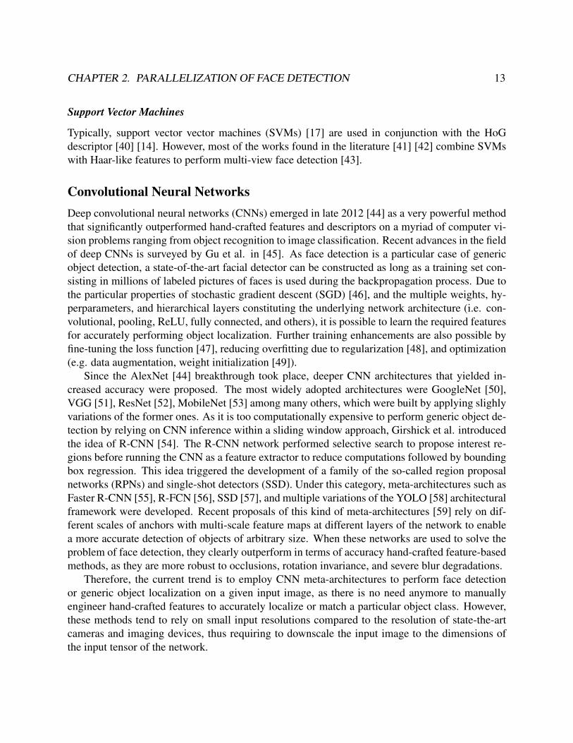
This thread imbalance bottleneck significantly degrades performance and is inherent to thecascade structure evaluation strategy. Hence, it does not depend on the particular hand-craftedfeature used within the classifier. However, in cases in which the boosting algorithm producesa cascade lacking stage thresholding values [70], and stage scores are accumulated through thecascade evaluation process, it is possible to apply thread rearrangement techniques. For instance,the cascade evaluation process could be split into m kernels (ki), where 0 ≤ i ≤ m − 1. Thefirst kernel (k0) could compute only the first n classifiers of the cascade, as they are the mostdiscriminative, and trigger the highest rejection rates. At this point, surviving threads obtained afterhaving executed the k0 kernel could be enqueued or grouped together with its (x, y) coordinatesfor further evaluation in the k1 kernel. This strategy goes on until all threads die or reach the endof the cascade in kernel km−1 (see Figure 2.3).
Therefore, the SIMD lanes in the k0 kernel would reach a higher occupancy than simply byapplying the naive parallelization pattern in which the input image is fully evaluated within a sin-gle kernel. However, the main drawback of thread rearrangement is that it is only easily splittableinto several kernels when the boosted cascade of classifiers strictly follows the soft cascade ap-proach [29]. More precisely, when the cascade is trained as a single large stage populated by weak

CHAPTER 2. PARALLELIZATION OF FACE DETECTION 17
classifiers rather than a sequence of stages, in which each one is constituted by a collection of weakclassifiers (shown in Figure 2.4). For this latter cascade structure, each stage yields a different scoreresponse after having completely evaluated its inner sequence of weak classifiers.
Consequently, thread rearrangement is severely constrained by the decision to be made at theend of each stage (di ellipses depicted in Figure 2.4). Depending on the depth and the quantity offeatures constituting a given stage of the conventional cascade, most threads processing adjacentpixels may finish early, but they would need to stall or wait at the decision node for the completionof threads that are still computing features in the same stage due to the SIMD paradigm. This factmeans that it is only feasible to split the evaluation of conventional cascades into kernels at thedecision nodes or study alternative parallelization strategies.
2.3 ConclusionsIn this chapter, we have reviewed the most widely used techniques for performing face detectionin images ranging from methods based on boosted classifiers of hand-crafted features to the latestCNN architectures. Currently, the parallelization of CNN inference is a well-studied problem, andstate-of-the-art libraries [67] and toolboxes [71] [72] already implement low-level optimizationsfor speeding up this process.
However, the low-level parallelization of cascades of hand-crafted features may still prove tobe relevant in scenarios in which the latency of face detection is critical, such as in the automatedreal-time surveillance of highly crowded locations. Other approaches could involve the usage ofhand-crafted features as a pre-processing step for quickly discarding image regions not containingfaces, and thus reduce the computational burden of inferencing a large resource-intensive CNNmeta-architecture.
Finally, such hybrid methods combining hand-crafted features with highly accurate CNNs, mayalso be adopted in scenarios in which power consumption is an issue. For instance, hand-craftedmethods could be dynamically scheduled in a SoC when battery power is too low, as it typicallydissipate less energy (<1 nJ/pixel) than widely adopted deep CNN architectures [73] [74].

18
Chapter 3
Efficient Evaluation of Cascades of BoostedEnsembles on GPU Architectures
State-of-the-art smart vision systems nowadays rely on deep convolutional neural networks (CNNs)for performing tasks such as highly accurate object localization, classification or segmentation,among others. Nevertheless, before the CNN revolution was triggered by the seminal AlexNetarchitecture [44], it was common to rely on hand-crafted computer vision techniques for perform-ing feature extraction, and later conduct classification tasks either by relying on ensemble learningmethods (e.g. boosting, random decision forests) or support vector machines (SVMs).
On the particular case of face detection, arguably the most widely adopted framework was thecascaded method introduced by Viola and Jones [8], [75], which optimally combined integral im-ages with Haar-like features of growing complexity learned by the AdaBoost [9] algorithm. Suchframework, heavily influenced subsequent hand-crafted object localization methods, as the cascadestructure derived from a boosting machine learning algorithm efficiently enables the early discardof image regions not containing the desired object classes. Multiple variations of the cascaded facedetection relied on more advanced features such as scale-invariant features (SIFT) [76], speeded uprobust features (SURF) [11], local binary patterns (LBP), histograms of oriented gradients (HoG)[30], and integral channel features (ICF) [12] among others, in order to dramatically improve theaccuracy of localization.
Although these methods are less accurate than current deep CNN meta-architectures, they arestill used in many use cases due to the lower computational footprint [73]. On top of that, it isdebatable whether the simpler, lightweight and pruned CNNs optimized to reduce computations tothe minimum extent for embedded devices are as accurate as ensemble methods based on hand-crafted features when detecting faces in images [77].
On the other hand, the unprecedented growth in user-generated multimedia content that weare experiencing during this decade is pushing the demand of computing performance to the limit.Today, some of the most advanced clusters and supercomputers rely on hybrid nodes that combinemassively parallel GPUs with multicore CPUs for processing this vast amount of data [78]. Thissituation will be even more challenging when the online services that run on datacenters enableend users the possibility to conduct computationally intensive interactive queries based on object

CHAPTER 3. EFFICIENT EVALUATION OF CASCADES OF BOOSTED ENSEMBLES 19
recognition or scene understanding on a collection of archived videos. A common way to re-duce both the latency and energy consumption of interactive queries is to implement these tasks inmultithreaded data-parallel accelerators such as GPUs, which are highly efficient in terms of per-formance per watt, as they yield more performance with less energy consumed per floating-pointoperation when compared to high-end multicore CPUs [79].
Ensemble methods progressively select combinations of low-level image features to build weakclassifiers based on how well the features discriminate between positive and negative samples.Due to the properties of boosting, the resulting classifier cascade behaves as a standalone strongclassifier, even though it was originally trained as a combination of weak hypotheses. The ideaof structuring classifiers in the form of a cascade enables early discarding of image regions thatare not prone to contain the desired object class, thus avoiding unnecessary computations. Furtherreductions in computations are achieved through the usage of a summed area table [10], [80] oran integral image. Variations of this framework with more sophisticated boosting algorithms [29],[70] and low-level image features are possible, but essentially they all expose the same challengeswhen ported to GPU architectures.
First, the dynamic resizing of the sliding window required for detecting objects of any sizeyields a low ALU occupancy if threads are directly mapped to different sliding windows. This isespecially true for larger sliding windows, which trigger the evaluation of cascade classifiers usingfew threads. Similarly, when smaller sliding windows scan the input image using features withminimal dimensions (i.e. the sample size used during the learning process), the GPU occupancyis maximized. This unbalanced distribution of work may potentially reduce performance shouldremain unaddressed.
Second, the irregular control flow derived from the evaluation of the classifier cascade couldproduce a situation in which a great proportion of GPU threads are divergent. When the executionpath of threads within a warp are not equal, threads taking different paths are serially executed, andmay negatively affect computational performance. Therefore, the cascade should keep the highestpossible rejection rates at the initial stages of the classifier to both reduce the impact of threaddivergence and increase the underlying throughput.
Considering that the growing trend in the HPC industry is to devote a larger amount of the diearea in several parallel processing units, usually structured among blocks of multithreaded SIMDlanes and private local caches, the problem of efficiently evaluating cascades of classifiers in sucharchitectures is still relevant. Even though object detection algorithms benefit from the data-levelparallelism inherently derived from pixels, additional strategies are required for further increasingcomputational performance during the feature evaluation process.
3.1 Pipeline for Ensemble Methods based on Integral ImagesTypically, an object detection pipeline starts from an input image or video frame. As it is nowcommon to have an on-die hardware video decoder on most SoCs and discrete GPUs, time con-suming tasks such as the video decoding of streams encoded with widely adopted codecs (e.g.H.264 [81], HEVC [82] or AV1 [83]) can be offloaded at the slice level to this fixed function logic.
CHAPTER 3. EFFICIENT EVALUATION OF CASCADES OF BOOSTED ENSEMBLES 20
Integral Image
Parallel Pre x Sum
Matrix Transposition
Parallel Pre x Sum
Matrix Transposition
1
2
3
4
Video Frame
Display
Cascade EvaluationScalingVideo Decoding Filtering
OpenGLTexture
OpenGLTexture
N
N
On-die HardwareVideo Decoder
tex2d() Texture Fetching
CUDA / OpenGL Map
Concurrent Execution of CUDA Kernels
CUDA / OpenGL Unmap
N N
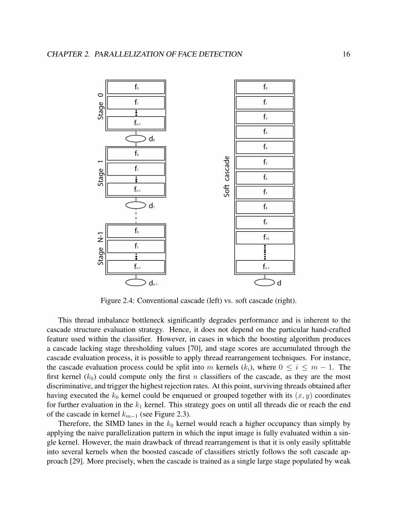
Figure 3.1: Proposed object detection pipeline for analyzing video streams.
When the video decoding stage is performed on a discrete GPU, the latency of memory transfersbetween CPU and GPU address spaces is significantly reduced due to the fact that these transfersdeal with compressed video frames. Through the usage of GPU hardware video decoding APIs[84], decompressed video frames are then directly mapped to a texture for further processing anddisplay enclosed objects to end users.
As certain hand-crafted features (e.g. Haar-like, ICF, SURF) require integral images [85] orsummed area tables [10] for speeding up computations, a generic facial localization pipeline tar-geting cascades of boosted ensembles must also perform fine-grained thread level parallelizationof such time-consuming computations. Rather than computing integral images by means of se-rialized aggregated additions, as Hensley et al. [80] pointed out, it is possible to parallelize thecomputation of integral images in O(n log2 n) steps by means of parallel horizontal and verticalprefix sum using data-parallel operations on graphics hardware. This is possible because moderngraphics hardware closely resembles a parallel machine of n processors, and enables recursivedoubling [86] techniques. Our proposed face detection pipeline shown in Figure 3.1 relies insteadon parallel prefix sum and parallel matrix transpositions to improve data locality in the on-diescratchpad memories available on GPUs.
Due to the fact that boosted cascades of features are trained for detecting faces at a given res-olution (typically, a dimension of 24x24 pixels), in order to detect faces of arbitrary size, it isrequired to downscale and filter multiple times the input video frame before computing integralimages. Other alternatives rely instead on directly building a gaussian pyramid [87] of the inputvideo frame and later computing a single integral image. Additionally, it is also possible to trainseveral cascades of classifiers to detect faces of specific growing dimensions, ranging from 24x24pixels up to the size of the image. All these strategies in fact require a fixed-sized sliding windowduring the evaluation stage of the boosted cascade of classifiers. However, there exists the possibil-ity of dynamically adjusting granularity by resizing the sliding window when using scale-invariantfeatures and a single boosted cascade of classifiers (see Figure 3.2). This variable-sized sliding

CHAPTER 3. EFFICIENT EVALUATION OF CASCADES OF BOOSTED ENSEMBLES 21
Variable-sized sliding window Fixed-sized sliding window
Threadxy
Threadx’y’Threadxy
Thread x’’y’’
Figure 3.2: Different strategies for evaluating features in boosted cascades of classifiers.
window has an impact on the classifier accuracy while yielding a low ALU occupancy on GPUs.More particularly, the potential number of simultaneous computing thread blocks nthb evaluatingWw ×Wh sliding windows on a given Iw × Ih integral image is substantially increased (Equation3.1) when image dimensions correspond to high definition (HD) or ultra-high definition (UHD)resolutions (i.e. 1080p, 4K and beyond).
nthb =
⌈Iw · IhWw ·Wh
⌉(3.1)
This latter behavior is depicted in Figure 3.3, which illustrates that only the smaller slidingwindow scales yield theoretically enough quantities of potential threads to keep ALUs with enoughamount of work, especially for high-end discrete GPUs, which include thousands of ALUs on die.This assumption is based on the model previously validated by Guz et al. [88], which proved thatthe occupancy η of cores Ncores in many-thread multiprocessors is bounded by:
η = min
1,nthreads
Ncores ·(
1 + tavg · rmCPIexec
) where 0 ≤ η ≤ 1 (3.2)
As the minimum in Equation 3.2 shows, there is no gain in creating and issuing more threads(nthreads) when the execution units are saturated (it is bounded by one). On the other hand, addi-tional threads must be issued when stalled threads are waiting data from the memory hierarchy toavoid the underutilization of the ALUs included in GPU cores. In the interest of correctly mod-eling this behaviour, Equation 3.2 also takes into account the rm ratio of memory instructions asa percentage of total instructions, the average tavg time in cycles to access data, and the averageCPIexec number of cycles required to execute an instruction.
Given that modern GPUs architectures such as NVIDIA’s Pascal [89] and Volta [90] typicallyconsume between 4 and 6 clock cycles on average for executing most integer and single-precisionfloating point instructions [91] (see Table 3.1), and assuming 400 clock cycles of latency when

CHAPTER 3. EFFICIENT EVALUATION OF CASCADES OF BOOSTED ENSEMBLES 22
Figure 3.3: Potential GPU threads resident in multiprocessors vs. sliding window dimensions
accessing the off-die memory (worst case scenario), Figure 3.3 shows the upper thread bounds formultiple values of Ncores achieving the maximum theoretical occupancy (η = 1 for rm = 0.5).
Therefore, for the sake of increasing the utilization of the GPU to the maximum extent, itis required to downscale the input video frame and filter it several times, before performing thecomputation of the subsequent integral images. Moreover, the pipeline starts with a given decodedvideo frame and it is then mapped to a texture, which leverages the GPU texture cache for speedingup downscaling and filtering stages (see Figure 3.1). At this point, the scaling stage generates Nresized images after subsampling decompressed frames stored in texture memory. As long as thismemory is indexed by floating point coordinates, it is possible to configure it for performing texturefetches with linear interpolation by relying on tex2D() instructions [5]. The filtering stage of thepipeline is necessary to avoid aliasing effects produced during the scaling stage, and thus preservethe original properties of the underlying image signal. After this stage has been completed, integralimages are computed by exploiting multiple levels of parallelism with a combination of parallelprefix sum and matrix transposition operations, as it was described earlier. By using this approach,

CHAPTER 3. EFFICIENT EVALUATION OF CASCADES OF BOOSTED ENSEMBLES 23
GPU Architecture Instructions Latency (cycles)
BFE, BFI, IADD, IADD32I,FADD, FMUL, FFMA,FMNMX, HADD2, HMUL2,HFMA2, IMNMX, ISCADD,LOP, LOP32I, LOP3, MOV,MOV32I, SEL, SHL, SHR,VADD, VABSDIFF, VMNMX,XMAD
6
Pascal DADD, DMUL,DFMA, DMNMX
8
FSET, DSET, DSETP,ISETP, FSETP
12
POPC, FLO, MUFU, F2F,F2I, I2F, I2I
14
IMUL, IMAD ∼86
IADD3, SHF, LOP3, SEL,MOV, FADD, FFMA,FMUL, ISETP, FSET, FSETP
4
IMAD, FMNMX,DSET, DSETP
5
Volta HADD2, HMUL2, HFMA2 6
DADD, DMUL, DFMA 8
POPC 10
FLO, BREV, MUFU 14
Table 3.1: Latency in clock cycles of assembly instructions in Pascal and Volta architectures.
coarse-grained parallelism is exploited through concurrently executing the kernels that implementsuch operations for each one of the considered scales. Fine-grained parallelism is subsequentlyexploited at thread-level within each kernel. Finally, the object detection pipeline concludes withthe evaluation of the boosted cascade of classifiers from integral images. This stage is the mostresource-intensive, as it must process integral images, and also exploits two degrees of parallelism.From a low-level perspective, a divide and conquer strategy must be used for evaluating the cascadewithin a kernel. Therefore, the analysis of the input integral image is performed by splitting it intoequally-sized blocks corresponding to a different fixed-sized sliding window. By following thisparallelization pattern, objects of multiple sizes are thus detected by concurrently executing thesame kernel for each integral image corresponding to a different scale. After all previous stagesconclude, the final outcome of the cascade evaluation stage is used for bounding regions in theoriginal video frame, which is finally mapped into an OpenGL [92] texture for display purposes.
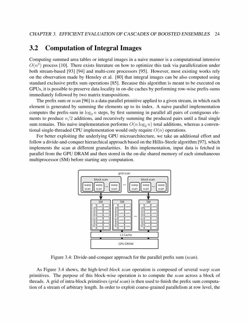
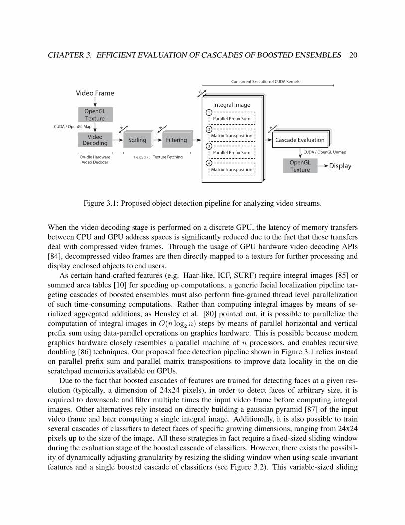
CHAPTER 3. EFFICIENT EVALUATION OF CASCADES OF BOOSTED ENSEMBLES 24
3.2 Computation of Integral ImagesComputing summed area tables or integral images in a naive manner is a computational intensiveO(n2) process [10]. There exists literature on how to optimize this task via parallelization underboth stream-based [93] [94] and multi-core processors [95]. However, most existing works relyon the observation made by Hensley et al. [80] that integral images can be also computed usingstandard exclusive prefix sum operations [85]. Because this algorithm is meant to be executed onGPUs, it is possible to preserve data locality in on-die caches by performing row-wise prefix-sumsimmediately followed by two matrix transpositions.
The prefix sum or scan [96] is a data-parallel primitive applied to a given stream, in which eachelement is generated by summing the elements up to its index. A naive parallel implementationcomputes the prefix-sum in log2 n steps, by first summing in parallel all pairs of contiguous ele-ments to produce n/2 additions, and recursively summing the produced pairs until a final singlesum remains. This naive implementation performs O(n log2 n) total additions, whereas a conven-tional single-threaded CPU implementation would only require O(n) operations.
For better exploiting the underlying GPU microarchitecture, we take an additional effort andfollow a divide-and-conquer hierarchical approach based on the Hillis-Steele algorithm [97], whichimplements the scan at different granularities. In this implementation, input data is fetched inparallel from the GPU DRAM and then stored in the on-die shared memory of each simultaneousmultiprocessor (SM) before starting any computation.
warpscan
warpscan
... warpscan
block scan
warpscan
warpscan
... warpscan
block scan...
grid scan
L2 Cache
GPU DRAM
shar
ed m
emor
y
SMcore core
core core
core core
core core
...
shar
ed m
emor
y
SMcore core
core core
core core
core core shar
ed m
emor
y
SMcore core
core core
core core
core core
Figure 3.4: Divide-and-conquer approach for the parallel prefix sum (scan).
As Figure 3.4 shows, the high-level block scan operation is composed of several warp scanprimitives. The purpose of this block-wise operation is to compute the scan across a block ofthreads. A grid of intra-block primitives (grid scan) is then used to finish the prefix sum computa-tion of a stream of arbitrary length. In order to exploit coarse-grained parallelism at row level, the
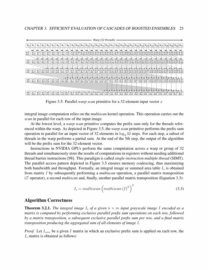
CHAPTER 3. EFFICIENT EVALUATION OF CASCADES OF BOOSTED ENSEMBLES 25
∑3 ∑27∑20∑19 23 ∑22 ∑23 ∑24 ∑25∑1821∑16∑15∑1417∑13∑11∑10 ∑28316∑1∑00 1 2 3 4 5 7 8 9 10 11 12 13 14 15 16 18 19 20 22 24 25 26 27 28 29 30∑0 ∑2 ∑4 ∑5 ∑6 ∑7 ∑8 ∑9 ∑12 ∑17 ∑21 ∑26∑0∑0
x0 x1 x2 x3 x4 x5 x6 x7 x8 x9 x10 x11 x12 x13 x14 x15 x16 x17 x18 x19 x20 x21 x22 x23 x24 x25 x26 x27 x28 x29 x30 x31
∑0 ∑1 ∑2 ∑3 ∑4 ∑5 ∑6 ∑7 ∑8 ∑9 ∑10 ∑11 ∑12 ∑13 ∑14 ∑15 ∑16 ∑17 ∑18 ∑19 ∑20 ∑21 ∑22 ∑23 ∑24 ∑25 ∑26 ∑27 ∑28 ∑29∑00 1 2 3 4 5 6 7 8 9 10 11 12 13 14 15 16 17 18 19 20 21 22 23 24 25 26 27 28 29 30 ∑3031
∑0 ∑6 ∑10 ∑20∑19∑18∑14 ∑22 ∑2330106 ∑3∑1∑00 1 2 3 4 5 7 8 9 11 12 13 14 15 16 17 18 19 20 21 22 23 24 25 26 27 28 29∑0 ∑2 ∑4 ∑5 ∑7 ∑8 ∑9 ∑11 ∑12 ∑13 ∑15 ∑16 ∑17 ∑21∑0∑0∑0∑0∑0∑0 ∑2431
∑0 ∑6 ∑10 ∑14 30106 ∑3∑1∑00 1 2 3 4 5 7 8 9 11 12 13 14 15 16 17 18 19 20 21 22 23 24 25 26 27 28 29∑0 ∑2 ∑4 ∑5 ∑7 ∑8 ∑9 ∑11 ∑12 ∑13 ∑15 ∑16∑0∑0∑0∑0∑0∑0 31∑0 ∑0∑0∑0∑0∑0∑0
30106 ∑00 1 2 3 4 5 7 8 9 11 12 13 14 15 16 17 18 19 20 21 22 23 24 25 26 27 28 29∑0∑0∑0∑0∑0∑0∑0 31∑0 ∑0∑0∑0∑0∑0∑0∑0 ∑0 ∑0∑0∑0∑0∑0 ∑0 ∑0∑0∑0∑0∑0 ∑0∑0∑0∑0
Warp (32 threads)
Figure 3.5: Parallel warp scan primitive for a 32-element input vector x
integral image computation relies on the multiscan kernel operation. This operation carries out thescan in parallel for each row of the input image.
At the lowest level, a warp scan primitive computes the prefix sum only for the threads refer-enced within the warp. As depicted in Figure 3.5, the warp scan primitive performs the prefix sumoperation in parallel for an input vector of 32 elements in log2 32 steps. For each step, a subset ofthreads in the warp performs a partial sum. At the end of the 5th step, the output of the algorithmwill be the prefix sum for the 32-element vector.
Instructions in NVIDIA GPUs perform the same computation across a warp or group of 32threads and simultaneously store the results of computations in registers without needing additionalthread barrier instructions [98]. This paradigm is called single-instruction multiple thread (SIMT).The parallel access pattern depicted in Figure 3.5 ensures memory coalescing, thus maximizingboth bandwidth and throughput. Formally, an integral image or summed area table Is is obtainedfrom matrix I by subsequently performing a multiscan operation, a parallel matrix transposition(T operator), a second multiscan and, finally, another parallel matrix transposition (Equation 3.3):
Is = multiscan(multiscan (I)T
)T(3.3)
Algorithm CorrectnessTheorem 3.2.1. The integral image Is of a given n × m input grayscale image I encoded as amatrix is computed by performing exclusive parallel prefix sum operations on each row, followedby a matrix transposition, a subsequent exclusive parallel prefix sum per row, and a final matrixtransposition producing the aggregated sum of all elements of image I .
Proof. Let Iexec be a given I matrix in which an exclusive prefix sum is applied on each row, theIs matrix is obtained as follows:

CHAPTER 3. EFFICIENT EVALUATION OF CASCADES OF BOOSTED ENSEMBLES 26
Iexc =
0 i00 i00 + i01 · · · (i00 + i00 + i01 + · · ·+ i0m−2)0 i10 i10 + i11 · · · (i10 + i10 + i11 + · · ·+ i1m−2)...
...... . . . ...
0 in−10 in−10 + in−11 · · · (in−10 + in−10 + in−11 + · · ·+ in−1m−2)
=⇒
ITexc =
0 0 · · · 0i00 i10 · · · in−10
i00 + i01 i10 + i11 · · · in−10 + in−11...
... . . . ...(i00 + · · ·+ i0m−2) (i10 + · · ·+ i1m−2) · · · (in−10 + · · ·+ in−1m−2)
=⇒
I ′ = ITexc =⇒
I ′exc =
0 0 0 · · · 00 i00 i00 + i10 · · · (i00 + · · ·+ in−20)...
...... . . . ...
(i00 + · · ·+ i0−m2) (i00 + · · ·+ i0m−2)0 (i00 + · · ·+ i0m−2) + · · ·+ · · · + · · ·+
(i10 + · · ·+ i1m−2) (in−20 + · · ·+ in−2m−2)
=⇒
Is = I ′Texc =⇒
Is =
0 0 · · · 00 i00 · · · i00 + · · ·+ i0m−2...
... . . . ...(i00 + · · ·+ i0m−2)
0 (i00 + · · ·+ in−20) · · · + · · ·+(in−20 + · · ·+ in−2m−2)
Transposing the matrices is necessary to avoid column-wise scanning, so that data localityis better exploited when accessing the shared memory. Memory coalescing and bulk transfers arerequired to achieve the maximum bandwidth for the GPU, so a natural way of transposing matricesis to divide them into equally-sized blocks and to copy data from the off-chip DRAM to the on-dieshared memories. This involves using a barrier instruction after data is transferred to the sharedmemory of each SM. Synchronization is required to guarantee that all threads constituting theCUDA block start with the transposition immediately after all memory transfers have concluded.

CHAPTER 3. EFFICIENT EVALUATION OF CASCADES OF BOOSTED ENSEMBLES 27
Algorithm 1: INTEGRALIMAGE
Data: Matrices I , Is of size W ×Hbegin
for i← 0 to H − 1 parallel doIs[i][0]← EXCLUSIVEPREFIXSUMKERNEL(I[i][0],W )
endI ′s ← MATRIXTRANSPOSITIONKERNEL(Is)
for i← 0 to H − 1 parallel doI ′′s [i][0]← EXCLUSIVEPREFIXSUMKERNEL(I ′s[i][0],W )
endIs ← MATRIXTRANSPOSITIONKERNEL(I ′′s )
end
Generally, the input matrix I is not a multiple of the warp width. To solve this issue, beforetransferring memory from the CPU address space to the GPU, the matrix must be zero-padded untilbecoming square. Even though this padding process causes additional memory transfers, the finalthroughput of the transposition will be higher, because all accesses will be properly coalesced andaligned. Algorithm 1 summarizes the process of computing the integral image, which internallyrelies on per-row exclusive parallel prefix sum kernels (i.e. multiscan), and the parallel matrixtransposition kernel.
Kernel (s1)
Kernel (s4)
Kernel (s3)
Kernel (s2)
Kernel (s1) Kernel (s4)
Kernel (s3)
Kernel (s2)Tim
e
GPU occupancy GPU occupancy
Figure 3.6: Serial (left) vs. Concurrent (right) kernel execution
As Figure 3.6 depicts, a given kernel si may not yield enough computations for keeping theunderlying GPU hardware resources busy. For avoiding to keep ALUs idle, it is worth to rely on thestrategy of concurrently issuing and executing several kernels. Therefore, the multiscan approach,which simultaneously executes parallel prefix sum kernels on each row of the input matrix, is theoptimal choice for reducing the execution time of integral image computations to the minimumextent.

CHAPTER 3. EFFICIENT EVALUATION OF CASCADES OF BOOSTED ENSEMBLES 28
3.3 Parallel Evaluation of Boosted Cascades of EnsemblesA typical object detection framework based on integral images must perform an exhaustive eval-uation of a boosted cascade of ensembles organized in stages containing an increasingly largernumber of features. In order to detect objects of any size at multiple locations, a kernel imple-menting such cascade evaluation not only has to test all integral image pixels, but also considerall possible sliding window dimensions and locations. This algorithm could also be significantlyimproved by performing rotations of the integral image (assuming scale invariant features), thusexponentially increasing the required amount of computations. Due to the particular propertiesof boosting algorithms, the traversal of the cascade data structure may be constrained by the de-pendencies between stages, and must be sequentially evaluated for each candidate window. Forthese reasons, we propose a parallelization pattern, where each integral image Is corresponding toa different downscaled video frame is divided into small and equally-sized n×m chunks.
Each chunk is directly mapped into a different thread block B(i, j), which is then scheduledto a streaming multiprocessor (SM). Let M be the memory chunk to be transferred to a SM, thepixels of a given integral image Is to be transferred by a given (x, y) thread of an n × m threadblock B(i, j) are determined by the following expressions (Equations 3.4 to 3.7):
M(x, y) = Is(α, β) (3.4)
M(x+ n, y) = Is(α + n, β) (3.5)
M(x, y +m) = Is(α, β +m) (3.6)
M(x+ n, y +m) = Is(α + n, β +m) (3.7)
Where α = i · n + x and β = j · m + y. According to these definitions, each thread of theblock will bring 4 pixels of the integral image to the shared memory, where 3 of them will be ofmemory regions meant to be explored by contiguous blocks (see Figure 3.7). Additionally, theseaccess patterns are sequentially performed to ensure memory coalescing.
After these memory transfers have been completed (and hardened by a syncthreads()
barrier instruction), the next step of the algorithm is to evaluate the boosted cascade of ensembles.This evaluation is both an arithmetic and a memory intensive operation. For example, a givenboosted cascade of Haar-like features [8] would need to perform 18 memory accesses for the 2-rectangle feature and 27 memory accesses for the 3-rectangle feature.
Furthermore, a given rectangle of a Haar-like feature is defined by its (i, j) location within then × m fixed-sized sliding window, its w × h dimensions, and the 4 values of the integral imageused for computing the area, thus requiring 9 memory accesses. Additionally, it is also required toperform between 4 and 5 arithmetic operations to estimate the response for each feature. Therefore,the main objective is to reduce latency when fetching from memory all required feature attributes(i.e. dimensions, coordinates and weights) with the purpose of keeping the ALUs busy and thusmaximize throughput. A similar rationale should also be applied when evaluating other boostedcascades of ensembles based on more complex features (e.g. SURF, ICF) requiring integral images.

CHAPTER 3. EFFICIENT EVALUATION OF CASCADES OF BOOSTED ENSEMBLES 29
block (i, j) block (i, j+1)
block (i+1, j) block (i+1, j+1)
threadx,y
Stage 2
Stage 3
Stage 1
· · ·
Stage N
Classier Cascade
Evaluation Window
Figure 3.7: Evaluation of the classifier cascade of Haar-like features on a block thread.
In view of this particular information is continuously reused when evaluating the cascade fea-tures for each integral image element, the right approach would involve moving all features to theGPU constant memory [5] (read-only on-die memory available in CUDA-enabled devices) beforelaunching the evaluation kernels. Moreover, it is also expected that threads processing adjacentpixels start evaluating the cascade features at the same initial stage and diverge in later iterations.In this situation, the usage of the constant memory is appropriate due to the fact that is specificallydesigned for broadcasting values for all warp threads that simultaneously access the same memoryaddress. With the aim of maximizing the information stored in the constant memory, Haar-likefeatures can be stored in a compressed fashion. Since all bits of the thresholds, coordinates, di-mensions and weight values are not significant, we propose pruning and later storing them into16-bit words.
Referring again to Figure 3.1, the cascade evaluation kernel must be executed for each one ofthe N integral images to detect faces of any size. As each CUDA block in the cascade evaluationkernel is fine-tuned to exactly match the w×h dimensions of the trained object class, it is expectedthat smaller integral images would yield a very low ALU occupancy (see Figure 3.3). This prob-lem is addressed by exploiting inter-kernel coarse-grained parallelism. Therefore, concurrentlyexecuting the cascade evaluation kernel for each integral image increases the chance of achievingfull GPU occupancy on microarchitectures featuring high core counts.
The whole process is summarized in the kernel presented in Algorithm 2, which requires asan input two matrices: an Is integral image, and a pre-allocated R matrix for storing integersrepresenting the deepest stage of the cascade reached during evaluation by a given thread. Thedimensions of both matrices must be equal. Additionally, it also requires an F boosted cascade offeatures containing S stages. Early rejection of the cascade structure is enforced by accumulatingscores in v while evaluating features, and by checking this latter value against the θ threshold thatmust be manually set up in the face detection framework.

CHAPTER 3. EFFICIENT EVALUATION OF CASCADES OF BOOSTED ENSEMBLES 30
Algorithm 2: EVALUATECASCADEKERNEL
Data: Matrices Is, R of size W ×H , Matrix F of size Sbegin
i← blockIdx.x * blockDim.x + threadIdx.x
j ← blockIdx.y * blockDim.y + threadIdx.y
M [threadIdx.x][threadIdx.y] = Is[i+ j ∗W ]M [threadIdx.x + blockDim.x][threadIdx.y] = Is[i+ blockDim.x + j ∗W ]M [threadIdx.x][threadIdx.y + blockDim.y] = Is[i+ (j + blockDim.y) ∗W ]M [threadIdx.x + blockDim.x][threadIdx.y + blockDim.y] =
Is[i+ blockDim.x + (j + blockDim.y) ∗W ]
syncthreads()
v ← 0
for s← 0 to S − 1 dok ← EVALUATEFEATURE(F [s],M)v ← v + kif v ≥ θ then
breakend
endR[j ∗W + i] = v
end
The output of the concurrent execution of the cascade evaluation kernel is a collection of arrayswith the same dimensions as integral images, and stored in the global memory of the GPU addressspace (R matrix in Algorithm 2). Likewise, there will be Ri arrays, where 0 ≤ i < N , preciselymatching the N number of scales considered in the pipeline (see Figure 3.1). Each (x, y) elementof these Ri arrays is an integer that represents the deepest stage of the cascade reached during theevaluating process. Therefore, the image region enclosed in a sliding window starting at (x, y)coordinates would be considered as an object or face if the integer value stored at that positionequals the maximum depth of the cascade. The precise dimensions of the sliding window aredetermined by multiplying the downscaling factor by the normalized dimensions of the objectsthat have been used for training the cascade.
The abovementioned operations are implemented in the display kernel. This kernel is alsoconcurrently executed for each scale and encloses objects in a rectangle by updating the RGBvalues of the original input image or video frame. Finally, the RGB image is mapped into astandard texture for displaying it using the CUDA-OpenGL interoperability API [5], although itcould be also mapped to other rendering APIs such as Vulkan [99].

CHAPTER 3. EFFICIENT EVALUATION OF CASCADES OF BOOSTED ENSEMBLES 31
3.4 Experimental SetupWith regard to the evaluation of both performance and accuracy of our generic object detectionGPU-based implementation, we built a benchmark dataset by retrieving a collection of 10 videoscontaining faces from the iTunes Movie Trailers website [100] (see Table 3.2). All selected movietrailers featured a 1920x1080 resolution with an average bitrate of 9 Mbps and were originallycompressed using the H.264/AVC codec [81] in a QuickTime container format. The testing plat-form was equipped with a quad-core Intel Core i7-4770 3.40 GHz CPU, an NVIDIA GeForceGTX 1060 graphics card, and relied on the Linux kernel version 4.15. For the implementation ofthe GPU kernels, we targeted the CUDA Toolkit 10.0 and the sm 61 architecture. Since the on-dieGPU video decoder works with bitstreams, we relied on the libavformat library for demuxinginput videos. Then the demuxed H.264 video frames were enqueued and decoded using NVDEC[84] API callback functions, and finally mapped to a GPU pointer for conducting further processingwith CUDA kernels. Considering that the underlying hardware decodes frames in NV12 format,it is enough to consider only the initial array of luminance components as the input of the scalingprocess and subsequent pipeline stages.
Legend Trailer Name DurationA 21 Jump Street 2 min. 29 sB 50/50 2 min. 49 sC American Reunion 1 min. 53 sD Bad Teacher 2 min. 29 sE Friends With Kids 2 min. 28 sG One For The Money 2 min. 29 sH The Dictator 1 min. 48 sI Tim & Eric’s Billion Dollar Movie 2 min. 19 sJ Unicorn City 2 min. 7 sK What To Expect When You’re Expecting 2 min. 8 s
Table 3.2: Selected H.264 movie trailers
For measuring performance of the GPU kernels, we relied on the CUDA compute commandline profiler (nvprof). Unfortunately, the profiler does not allow gathering values from perfor-mance counters while concurrently executing kernels. To avoid kernel serialization, we enabledand disabled the --concurrent-kernels profiling directive between multiple executions. Theobjective was to capture the timestamps of kernels issued in different streams, while performingface detections in a video, so that we could determine whether they were effectively overlap-ping computations or not. Similarly, concurrent execution was deliberately disabled for measuringstatistics such as branch and control flow divergence in each streaming multiprocessor (SM).
For analyzing thread execution at the finest granularity possible and thus capture the innerworkings of the warp scheduler, we instrumented the cascade evaluation kernel using the GPUclock() function. Both the initial and final timestamps for each thread of the CUDA blockwere stored in a matrix. With this information, it is possible to quickly visualize which warpsare processing a given image region and make deductions about how the GPU schedules a grid ofCUDA thread blocks during kernel execution.
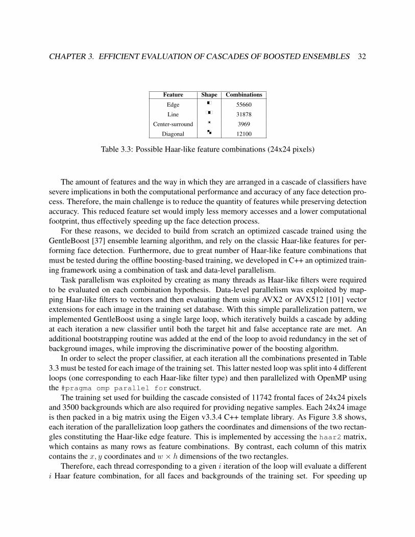
CHAPTER 3. EFFICIENT EVALUATION OF CASCADES OF BOOSTED ENSEMBLES 32
Feature Shape Combinations
Edge 55660
Line 31878
Center-surround 3969
Diagonal 12100
Table 3.3: Possible Haar-like feature combinations (24x24 pixels)
The amount of features and the way in which they are arranged in a cascade of classifiers havesevere implications in both the computational performance and accuracy of any face detection pro-cess. Therefore, the main challenge is to reduce the quantity of features while preserving detectionaccuracy. This reduced feature set would imply less memory accesses and a lower computationalfootprint, thus effectively speeding up the face detection process.
For these reasons, we decided to build from scratch an optimized cascade trained using theGentleBoost [37] ensemble learning algorithm, and rely on the classic Haar-like features for per-forming face detection. Furthermore, due to great number of Haar-like feature combinations thatmust be tested during the offline boosting-based training, we developed in C++ an optimized train-ing framework using a combination of task and data-level parallelism.
Task parallelism was exploited by creating as many threads as Haar-like filters were requiredto be evaluated on each combination hypothesis. Data-level parallelism was exploited by map-ping Haar-like filters to vectors and then evaluating them using AVX2 or AVX512 [101] vectorextensions for each image in the training set database. With this simple parallelization pattern, weimplemented GentleBoost using a single large loop, which iteratively builds a cascade by addingat each iteration a new classifier until both the target hit and false acceptance rate are met. Anadditional bootstrapping routine was added at the end of the loop to avoid redundancy in the set ofbackground images, while improving the discriminative power of the boosting algorithm.
In order to select the proper classifier, at each iteration all the combinations presented in Table3.3 must be tested for each image of the training set. This latter nested loop was split into 4 differentloops (one corresponding to each Haar-like filter type) and then parallelized with OpenMP usingthe #pragma omp parallel for construct.
The training set used for building the cascade consisted of 11742 frontal faces of 24x24 pixelsand 3500 backgrounds which are also required for providing negative samples. Each 24x24 imageis then packed in a big matrix using the Eigen v3.3.4 C++ template library. As Figure 3.8 shows,each iteration of the parallelization loop gathers the coordinates and dimensions of the two rectan-gles constituting the Haar-like edge feature. This is implemented by accessing the haar2 matrix,which contains as many rows as feature combinations. By contrast, each column of this matrixcontains the x, y coordinates and w × h dimensions of the two rectangles.
Therefore, each thread corresponding to a given i iteration of the loop will evaluate a differenti Haar feature combination, for all faces and backgrounds of the training set. For speeding up

CHAPTER 3. EFFICIENT EVALUATION OF CASCADES OF BOOSTED ENSEMBLES 33
#pragma omp parallel forfor(int i=0; i<haar2.rows(); i++)VectorXi eval(dataset.cols());eval = (-1) * (dataset.row(haar2(i,0)) +
dataset.row(haar2(i,1)) -dataset.row(haar2(i,2)) -dataset.row(haar2(i,3))) +
2 * (dataset.row(haar2(i,4)) +dataset.row(haar2(i,5)) -dataset.row(haar2(i,6)) -dataset.row(haar2(i,7)));
regression(eval, i);
Figure 3.8: Parallel loop for testing edge feature combinations.
· · ·
pixel 0pixel 1pixel 2
pixel 575pixel 574pixel 573
· · ·
pixel 0pixel 1pixel 2
pixel 575pixel 574pixel 57357
6 [2
4x24
]El
emen
ts
· · ·
pixel 0pixel 1pixel 2
pixel 575pixel 574pixel 573
· · ·
1 byte
Integral Images
VectorizedLOAD
Figure 3.9: Encoding used for the dataset matrix that stores the training set.
the evaluation process, the dataset matrix stores precomputed values of integral images of thetraining set rather than original pixel values.
The data-level parallelization pattern exploits the fact that, because all integral images have thesame dimension (24x24 pixels), it is then possible to encode each of them in a single column ofthe dataset matrix using 576 rows. Hence, this matrix will have as many columns as integralimages the training set has (see Figure 3.9). With this simple data transformation, filter responsesof each Haar-like feature to be tested are easily vectorized with AVX2 or AVX512 instructions(depending on the underlying CPU vector SIMD capabilities) through the overloaded arithmeticoperators provided by the Eigen C++ library.
At the end of the loop, the thread private eval vector is used for storing the result of theevaluation of the i Haar-like feature for the whole training set. Then, the regression function iscalled for estimating parameters of weak classifiers from the filter responses stored in eval.

CHAPTER 3. EFFICIENT EVALUATION OF CASCADES OF BOOSTED ENSEMBLES 34
Finally, when the four parallelized loops that test the different Haar-like feature types con-clude, a ranking function selects the weak classifier that best discriminates between faces andbackgrounds. This weak classifier is then added to the cascade, and the main external loop contin-ues until the target hit and false acceptance rate are achieved. Also, we selected the OpenCV frontalface feature set designed by Lienhart et al. [19] (named haarcascade frontalface alt2.xml) asa baseline for estimating the accuracy of the trained cascade.
To conduct the performance and profiling experiments described earlier, a full-blown GPU-based face detector framework was developed from scratch using a combination of C/C++ hostCPU code and CUDA kernels meant to be executed on the GPU (not to be confused with the CPU-based cascade training framework). Such GPU-based face detection software implements at thelow-level the pipeline shown in Figure 3.1, and more particularly, the CUDA cascade evaluationkernel proposed in Algorithm 2. Therefore, this framework accepts as a parameter a file contain-ing a boosted cascades of ensembles (see Figure 3.10), which facilitates the comparison betweencascades trained by us (encoded using our own KBZ proprietary binary format), and the frontalface detector XML cascades shipping in the standard distribution of OpenCV v4.2.
- CUDA Runtime Version 10000- Device 0# GeForce GTX 1060 [1.71 GHz - 10 Multiprocessors - sm_61 - 6077 MB]- Device 0# has been selected for CUDA computation
Usage: facedetector --image <image.jpg> --cascade <cascade.xml>facedetector --video <video.mp4> --cascade <cascade.xml>
Options: --video <video.mp4> Input video file--image <image.jpg> Input image file--cascade <cascade.kbz> Input cascade file (KBZ or XML)--output <image.ppm> Output image file--numscales <num> Number of scales considered--minscale <num> Minimum scale considered--maxscale <num> Maximum scale considered--mineyedist <num> Minimum eye distance--maxeyedist <num> Maximum eye distance--scaletype <[LINEAR | EXP | SINH]> Scaling algorithm--maxstages <num> Maximum number of stages--nonms Disable non-maximum suppression
Figure 3.10: Command line options of the developed GPU-based face detection framework.
This framework also outputs the input video feed on a window showing localized faces en-closed by a box, while performing non-maximum suppression (NMS) to select the best detectionamong all the candidates returned as an output by the CUDA cascade evaluation kernel.
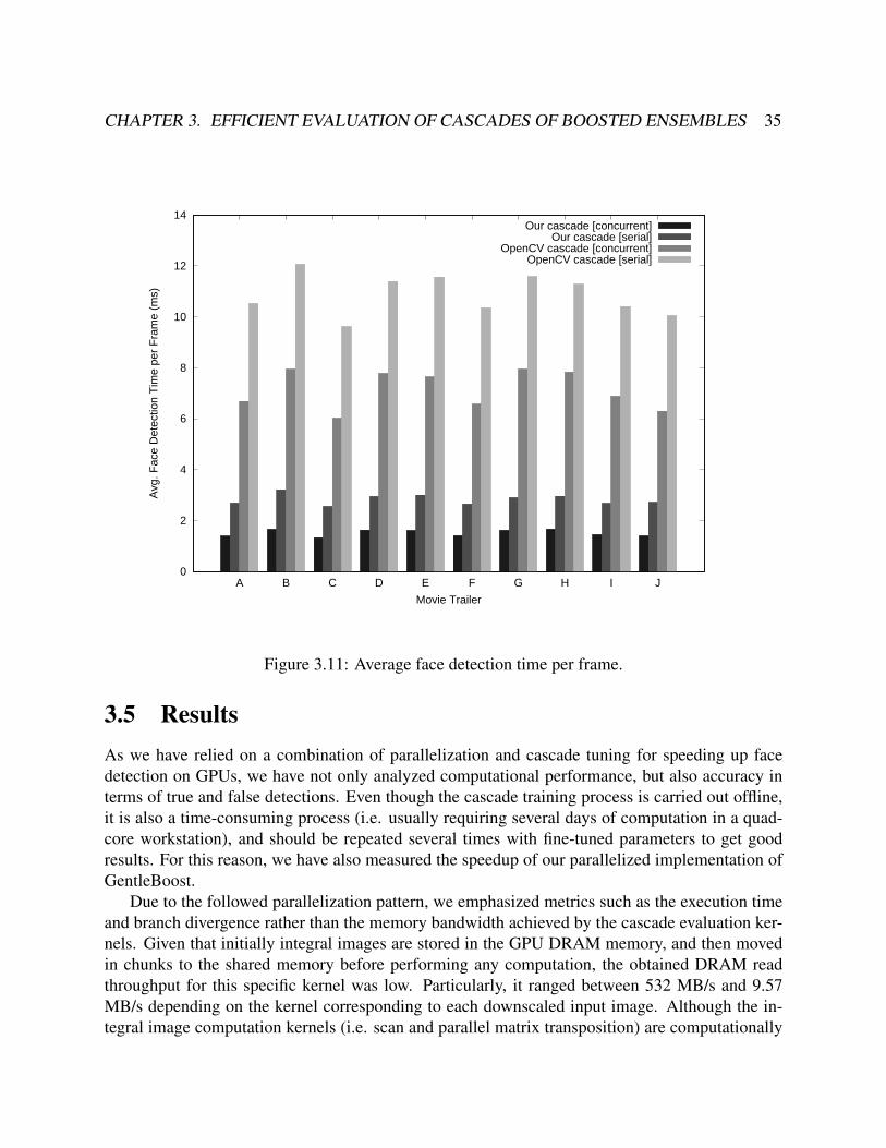
CHAPTER 3. EFFICIENT EVALUATION OF CASCADES OF BOOSTED ENSEMBLES 35
0
2
4
6
8
10
12
14
A B C D E F G H I J
Avg
. Fac
e D
etec
tion
Tim
e pe
r F
ram
e (m
s)
Movie Trailer
Our cascade [concurrent]Our cascade [serial]
OpenCV cascade [concurrent]OpenCV cascade [serial]
Figure 3.11: Average face detection time per frame.
3.5 ResultsAs we have relied on a combination of parallelization and cascade tuning for speeding up facedetection on GPUs, we have not only analyzed computational performance, but also accuracy interms of true and false detections. Even though the cascade training process is carried out offline,it is also a time-consuming process (i.e. usually requiring several days of computation in a quad-core workstation), and should be repeated several times with fine-tuned parameters to get goodresults. For this reason, we have also measured the speedup of our parallelized implementation ofGentleBoost.
Due to the followed parallelization pattern, we emphasized metrics such as the execution timeand branch divergence rather than the memory bandwidth achieved by the cascade evaluation ker-nels. Given that initially integral images are stored in the GPU DRAM memory, and then movedin chunks to the shared memory before performing any computation, the obtained DRAM readthroughput for this specific kernel was low. Particularly, it ranged between 532 MB/s and 9.57MB/s depending on the kernel corresponding to each downscaled input image. Although the in-tegral image computation kernels (i.e. scan and parallel matrix transposition) are computationally

CHAPTER 3. EFFICIENT EVALUATION OF CASCADES OF BOOSTED ENSEMBLES 36
10.559 10.56 10.561 10.562 10.563 10.564 10.565 10.566 10.567
Time (s)
Stre
ams
Figure 3.12: Execution trace of the cascade evaluation kernels (one for each considered scale) for agiven video frame of the 50/50 movie trailer. Kernels processing smaller image scales are executedcompletely overlapped for maximizing performance.
intensive, they only account on average for a 20% of the total face detection computation time.As Figure 3.11 shows, switching from serial to concurrent kernel execution doubles performancewhen detecting faces in video frames of the selected 1080p movie trailers. Therefore, the lowGPU occupancy achieved by serially executing the kernels corresponding to smaller scales is thuseffectively avoided when these scales are processed in parallel. The impact on performance ofoverlapping the cascade evaluation kernel computations for small scales is visible in the executiontrace depicted in Figure 3.12. This trace was produced by gathering the initial and final executiontimestamps of each kernel during profiling. Since each kernel is mapped into different CUDAstreams, the GPU scheduler is capable of issuing and executing thread instructions from differentCUDA kernels.
The obtained results also show that replacing the OpenCV feature dataset with our own cas-cade offers an additional 2.5X performance improvement. Therefore, the combined approach (i.e.concurrent execution using our cascade) offers a 5X speedup over the serial kernel execution of theOpenCV cascade. Although both cascades feature 25 stages, the OpenCV cascade has 2913 weakclassifiers, whereas ours has only 1446. As expected, this reduction in the Haar-like feature counttranslates in fewer computations and memory accesses thus reducing face detection latency.
It should be noted that Figure 3.11 represents only face detection elapsed time, and does nottake into account the H.264 video decoding latency. As it was previously discussed, this task iscompletely offloaded to the on-die GPU video decoder. For the selected movie trailers, the averagedecoding latency of a given frame ranged between 1 and 3 ms thus yielding an average throughputof 250 FPS when performing both tasks (i.e. video decoding and face detection) on the GPU.

CHAPTER 3. EFFICIENT EVALUATION OF CASCADES OF BOOSTED ENSEMBLES 37
As Figure 3.13 depicts, face detection latency per frame for a given movie trailer may expe-rience a huge variability. This latency basically depends on the number of faces that appear oneach video frame. Considering that both cascades were trained using backgrounds and other ob-jects as examples of non-faces, image regions not containing any faces are quickly rejected duringthe cascade evaluation process. Similarly, it also shows that the OpenCV cascade face detectionlatency pattern is quite similar to our cascade, but 4X slower when kernels are serially executed.This slowdown may be also noticeable when the H.264 video decoding latency is also consideredfor the concurrent OpenCV cascade evaluation.
Usually, thread divergence is one of the most undesired side effects that negatively affectsperformance when porting serial applications to the multithreaded SIMD architectures of modernGPUs. Due to the fact that each warp thread evaluates the cascade of classifiers for a differentsliding window, our proposed parallelization pattern may potentially yield a high percentage ofdivergent branches. Under this scenario, multiple threads of a warp could trigger an early exit atthe first stages of the cascade during the evaluation, while the others finish in deeper stages. Thissituation would force some warp threads to stall thus underutilizing GPU resources.
In order to determine the branch efficiency of the cascade evaluation kernel, we gathered theratio of non-divergent branches to total branches during execution using the GPU performancecounters. The obtained results showed that on average 98.9% of branches were non-divergent.
The reason for this behaviour is that when a given warp evaluates the boosted cascade of clas-sifiers, adjacent integral image elements mostly end at the same stage. As our parallel face detectorstores in the GPU global memory the deepest stage reached during the cascade evaluation process,we decided to keep this information saved in the CPU address space for all pixels and scales acrossall video frames. The purpose of this task was to study the distribution of the deepest stage reachedby all GPU threads when evaluating pixels of a given video frame for each considered scale.
Figure 3.14 shows the aggregated results obtained for all the video frames of a selected movietrailer. On average, a thread evaluating a window starting at a given (x, y) pixel yields a rejectionrate of 94.52% at the first stage of the cascade, and thus quickly discards non-face regions. Sim-ilarly, the average rejection rate for the second stage was 4%, and then it is dramatically reducedfor the remaining stages. The results for other movie trailers were virtually the same.
Additionally, we also evaluated the scalability of the parallelized cascade training algorithmunder two different SMP scenarios. In view of this process usually takes several days, we decidedjust to measure the speedup obtained in the first iteration of the main loop of the GentleBoost al-gorithm. Furthermore, since each iteration of the main loop must test all possible Haar-like featurecombinations for all input images, the performance improvement should be noticeable. This latterprofiling was unrelated to the cascade evaluation kernel, but it was useful for showing how theOMP NUM THREADS environment variable greatly affected the execution time of the cascade trainingprocess as the number of OpenMP CPU threads were increased. In that sense, the algorithm wasexecuted using as an input the image dataset previously described (i.e. pictures containing facesplus pictures not containing faces), and the number of threads modified between multiple runs bysetting the OMP NUM THREADS environment variable accordingly.

CHAPTER 3. EFFICIENT EVALUATION OF CASCADES OF BOOSTED ENSEMBLES 38
Concurrent
Serial
Concurrent
Serial
Figure 3.13: Face detection elapsed time per frame for the movie trailer B. The obtained resultsshow differences between serial (gray) and concurrent kernel execution (black) for two differentcascades: the OpenCV frontal feature set (top) and the cascade trained by us (bottom).

CHAPTER 3. EFFICIENT EVALUATION OF CASCADES OF BOOSTED ENSEMBLES 39
0,00001%
0,0001%
0,001%
0,01%
0,1%
1%
10%
100%
1
25
RejectionRate
Stages
Scales
Figure 3.14: Rejection rates for each cascade stage and image scale for the movie trailer K.
As Figure 3.15 depicts, the obtained speedup was close to 3.5X in both scenarios when theinner loops were parallelized with 8 threads. Although we executed the GentleBoost algorithm ona workstation equipped with an Intel Xeon Silver 4110 CPU, and compiled our training frameworkwith AVX512 SIMD vector instructions by relying on the Eigen C++ library, an older quad-coreIntel Core i7-4770 featuring AVX2 instructions outperformed the latter with a 2X performanceimprovement. This unexpected result was obviously due to the huge difference in clock frequenciesbetween both processors (2.10 GHz vs. 3.40 GHz).
Low-level MicrobenchmarkingFor understanding how the GPU schedules warps during the object detection process, we instru-mented the cascade evaluation kernel for a given image scale using our newly trained cascadefeature dataset. The selected image is depicted in Figure 3.17 and includes 44 faces. Even thoughthe original image has a resolution of 3504x2336 pixels, we executed the kernel with a 1175x800downscaled image to simplify the visualization process with a lower active thread count. Our ker-nel instrumentation mainly consisted in allocating two auxiliary matrices for storing timestamps ofeach block thread by calling the clock() function available in the CUDA runtime API. Firstly, bystoring the timestamp corresponding to the issuance of each thread by the underlying warp sched-ulers of each simultaneous multiprocessor (SM). Thereafter, the timestamp obtained at the endingof execution of each thread was also stored in the second matrix. In addition, concurrent kernel

CHAPTER 3. EFFICIENT EVALUATION OF CASCADES OF BOOSTED ENSEMBLES 40
Intel Xeon Silver 4110 @ 2.10 GHz Intel Core i7-4770 @ 3.40 GHz
Figure 3.15: Execution time for a single iteration of the parallelized version of GentleBoost ondifferent SMP scenarios, as the value of the OMP NUM THREADS environment variable is increased.
execution was deliberately disabled to correctly instrument the kernel with just one image scale.The latency in GPU clock cycles of each warp thread was determined by computing the differencebetween the initial and final execution timestamps for the biggest image scale. Then, the obtainedvalues were 2D spatially distributed according to the blockIdx, blockDim and threadIdx CUDAvariables, and GPU clock latencies encoded using a color scale. By relying on this methodol-ogy, we also generated a video, which is distributed as a supplementary material of this work, andclearly shows how warp threads are spatially scheduled across all pixels of the input image.
As it is shown in Figure 3.17, the cascade evaluation kernel latency ranged between 5500 and1.1 million cycles. Image regions depicted using a warmer color palette (i.e. red color) representareas populated with faces, thus taking substantially more GPU clock cycles to compute. There-fore, those warmer regions highlight the fact they reach the final stage of the boosted cascade ofclassifiers, so that the early discard of the cascade data structure is never triggered. Dimensions inpixels of the regular structures in the form of boxes were measured and corresponded to the dimen-

CHAPTER 3. EFFICIENT EVALUATION OF CASCADES OF BOOSTED ENSEMBLES 41
sions of the CUDA thread block (25x25). Similarly, the line structures that appear on the image arerelated to the GPU scheduler and seemed to correspond to different warps, given that the length inpixels of these lines is always 32 (i.e. the number of threads in a warp of the SIMT architecture).This fact is easily observable in Figure 3.16, which shows the evolution of thread processing fordifferent δt sequence intervals extracted from the timestamps gathered during microbenchmarking.
Over time, warp threads (i.e. horizontal color lines) trigger the creation of sliding windows toevaluate the boosted cascade of ensembles at each region, while progressing through the adjacentCUDA block threads, which are responsible for analyzing a different memory chunk M(x, y) ofthe input image (see the parallelization pattern depicted in Figure 3.7).
Figure 3.16: Detailed execution time lapse of the cascade evaluation kernel for an image chunk.
Referring again to Figure 3.17, it is also clear that warp threads taking longer clock cycles toexecute are closely related to image regions containing faces. Likewise, the obtained delay distri-bution is strongly biased towards low latency, which shows that the early discarding mechanismof the cascade of classifiers worked as it was initially expected. Furthermore, we determined that97.8% of measured latencies were less than 120,000 clock cycles, which essentially correspondsto just one tenth of the observed spectrum. These results are in line with the low divergence valuespreviously obtained.
The microbenchmarking visual approach presented in this chapter is completely agnostic of thelow-level computer vision features used in the cascade of boosted ensembles. Therefore, it couldbe easily implemented as a profiling tool for studying potential performance bottlenecks of anyGPU-based object localization framework based on boosting and sliding window image scanning.

CHAPTER 3. EFFICIENT EVALUATION OF CASCADES OF BOOSTED ENSEMBLES 42
5.5K cycles 1.1M cycles
Figure 3.17: Latency in clock cycles for each GPU thread (bottom) after having executed thecascade evaluation kernel on an image (top). Warp threads with the highest latency correspond toregions containing faces.
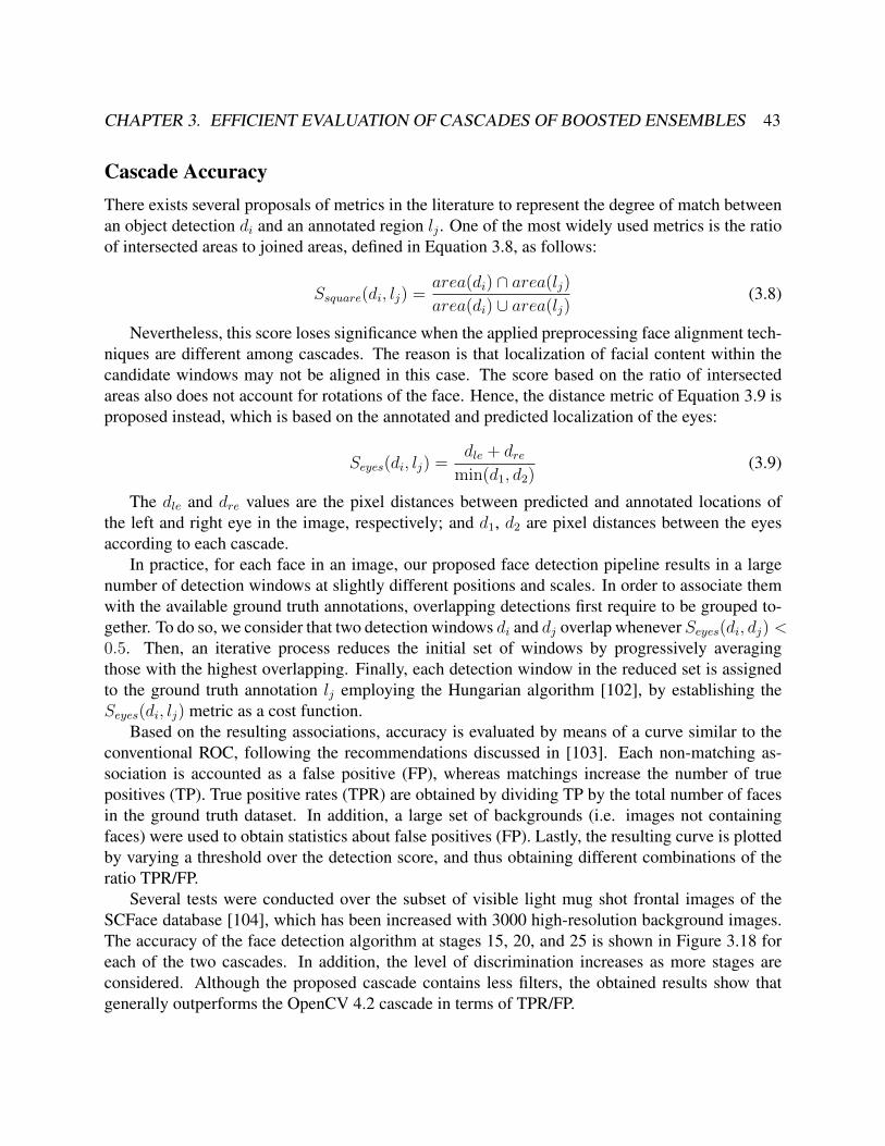
CHAPTER 3. EFFICIENT EVALUATION OF CASCADES OF BOOSTED ENSEMBLES 43
Cascade AccuracyThere exists several proposals of metrics in the literature to represent the degree of match betweenan object detection di and an annotated region lj . One of the most widely used metrics is the ratioof intersected areas to joined areas, defined in Equation 3.8, as follows:
Ssquare(di, lj) =area(di) ∩ area(lj)
area(di) ∪ area(lj)(3.8)
Nevertheless, this score loses significance when the applied preprocessing face alignment tech-niques are different among cascades. The reason is that localization of facial content within thecandidate windows may not be aligned in this case. The score based on the ratio of intersectedareas also does not account for rotations of the face. Hence, the distance metric of Equation 3.9 isproposed instead, which is based on the annotated and predicted localization of the eyes:
Seyes(di, lj) =dle + dre
min(d1, d2)(3.9)
The dle and dre values are the pixel distances between predicted and annotated locations ofthe left and right eye in the image, respectively; and d1, d2 are pixel distances between the eyesaccording to each cascade.
In practice, for each face in an image, our proposed face detection pipeline results in a largenumber of detection windows at slightly different positions and scales. In order to associate themwith the available ground truth annotations, overlapping detections first require to be grouped to-gether. To do so, we consider that two detection windows di and dj overlap whenever Seyes(di, dj) <0.5. Then, an iterative process reduces the initial set of windows by progressively averagingthose with the highest overlapping. Finally, each detection window in the reduced set is assignedto the ground truth annotation lj employing the Hungarian algorithm [102], by establishing theSeyes(di, lj) metric as a cost function.
Based on the resulting associations, accuracy is evaluated by means of a curve similar to theconventional ROC, following the recommendations discussed in [103]. Each non-matching as-sociation is accounted as a false positive (FP), whereas matchings increase the number of truepositives (TP). True positive rates (TPR) are obtained by dividing TP by the total number of facesin the ground truth dataset. In addition, a large set of backgrounds (i.e. images not containingfaces) were used to obtain statistics about false positives (FP). Lastly, the resulting curve is plottedby varying a threshold over the detection score, and thus obtaining different combinations of theratio TPR/FP.
Several tests were conducted over the subset of visible light mug shot frontal images of theSCFace database [104], which has been increased with 3000 high-resolution background images.The accuracy of the face detection algorithm at stages 15, 20, and 25 is shown in Figure 3.18 foreach of the two cascades. In addition, the level of discrimination increases as more stages areconsidered. Although the proposed cascade contains less filters, the obtained results show thatgenerally outperforms the OpenCV 4.2 cascade in terms of TPR/FP.
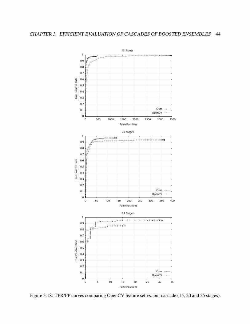
CHAPTER 3. EFFICIENT EVALUATION OF CASCADES OF BOOSTED ENSEMBLES 44
0
0.1
0.2
0.3
0.4
0.5
0.6
0.7
0.8
0.9
1
0 500 1000 1500 2000 2500 3000 3500
True
Pos
itive
Rat
e
False Positives
OursOpenCV
15 Stages
0
0.1
0.2
0.3
0.4
0.5
0.6
0.7
0.8
0.9
1
True
Pos
itive
Rat
e
False Positives
0 50 100 150 200 250 300 350 400
OursOpenCV
20 Stages
0 5 10 15 20 25 30 35 0
0.1
0.2
0.3
0.4
0.5
0.6
0.7
0.8
0.9
1
True
Pos
itive
Rat
e
False Positives
OursOpenCV
25 Stages
Figure 3.18: TPR/FP curves comparing OpenCV feature set vs. our cascade (15, 20 and 25 stages).
CHAPTER 3. EFFICIENT EVALUATION OF CASCADES OF BOOSTED ENSEMBLES 45
3.6 ConclusionsIn this chapter, we have presented a highly parallel GPU-based object detector that relies on classiclow-level Haar-like features for finding faces in videos. Our proposal heavily exploits concurrentkernel execution, local on-die caches, and a customized cascade for dramatically reducing the de-tection latency, while slightly improving the detection accuracy when compared to the frontal facedetection cascade shipped in OpenCV 4.2. The obtained results also show that the combinationof both techniques yields a 5X speedup over a conventional GPU implementation with serializedkernel execution.
Even though we have relied on our own cascade for achieving these results, the usage of con-current kernel execution with a fixed-sized sliding window has proven to be useful for increasingthe GPU occupancy of any cascade of boosted ensembles. Furthermore, we also presented a SMPparallel GentleBoost framework and its corresponding implementation that exploits both task anddata-level parallelism for reducing the duration of the cascade training process. With the combina-tion of OpenMP and AVX2/AVX512 vector extensions we showed that it was possible to obtain a3.5X speedup over the conventional serial implementation with little effort.
The proposed parallelization pattern and GPU cascade evaluation kernel enable the adaptationof our framework to other hand-crafted features that also work with integral images (e.g. integralchannel features (ICF) or speeded up robust features (SURF) among the most important ones).Although, it is also possible to exploit concurrent kernel execution for the evaluation of cascadesof ensembles not requiring integral images (e.g. histograms of oriented gradients, local binarypatterns or multi-block variants of both methods).
Finally, we have proved that it is feasible to mitigate the impact of thread divergence when usinga cascade of classifiers. By training from scratch a cascade with a high rejection rate on its firststage, non-face image regions are mostly rejected at this stage. As the obtained results have shown,high rejection rates and low thread divergence are strongly correlated. Moreover, this chapter alsoincluded a novel visualization technique based on microbenchmarking for studying at the lowestlevel how GPU clock cycles are spent when evaluating cascades. Such technique is useful also forgraphically determining how warps are spatially scheduled during the cascade evaluation kernelexecution. Therefore, this novel warp visualization technique opens the door to the development ofa software profiler plug-in for studying bottlenecks in object detection frameworks targeting GPUarchitectures. As supplementary material, we include a video depicting GPU warp schedulingover time when executing our parallel object detection framework using as an input a large picturecontaining dozens of faces.

46
Chapter 4
Face Localization in Ultra High DefinitionResolution Video Streams
In the last few years, the resolution and pixel densities of image CMOS sensors have experienceda dramatic boost. It is now not uncommon to find 4K resolution image CMOS sensors alreadyincluded in high-end smartphones, professional photo and video cameras or in automated opticalinspection industrial equipment. More recently, 8K image CMOS sensors have become available,and due to the improvements in the compression ratio of video codecs such as H.265/HEVC [82],[105] and AV1 [83], it is expected that workloads at such resolutions will become mainstream.
Furthermore, additional improvements in transistor count densities have enabled the emer-gence of ultra high resolution CMOS sensors featuring more than 100 million pixels. In 2017,Sony Corporation announced the IMX461 and IMX411 sensors, which feature an image capturingresolution of 100 and 150 megapixels, respectively. Similarly, Canon announced the availabilityof a 250-megapixel APS-H image CMOS sensor with low noise ratios (120MXS) [106], whichis expected to be included in upcoming professional cameras. Even Samsung has released a 100megapixel sensor for smartphones [107].
One application of high resolution CMOS sensors is large area surveillance at distant locations.The massive pixel densities and image resolutions may be leveraged for performing unconstrainedface identification of crowds in densely populated areas at very far distances from the camera. Asan example, Figure 4.1 highlights how high resolutions could be used for allowing the digital mag-nification of arbitrary regions within a wide area in a football stadium. Even though that is possibleto accurately localize and identify objects using a conventional Full HD (1080p) resolution, it isnot possible to keep the original image properties and quality after magnifying it. This zooming inprocess is absolutely required when the camera is located at far distances, and as a result of this,captured image frames are prone to blurring and distortion.
Hence, it is unclear how current face detection and localization frameworks based on region-proposal [55] [108] [56] and single-shot CNNs [57] are going to cope with increasing resolutions,while keeping a power/accuracy trade-off well enough for enabling inference at rates close to real-time speeds. An exhaustive benchmarking of the speed/accuracy trade-off of modern CNN-basedobject localization frameworks was conducted by Huang et al. in [109]. In this study, a high-end

CHAPTER 4. FACE LOCALIZATION IN UHD RESOLUTION VIDEO STREAMS 47
(a) Conventional 2-Megapixel image CMOS sensor (1920x1080 resolution)
(b) 120-Megapixel image captured by the Canon 120MXS CMOS sensor (13272x9176 resolution)
Figure 4.1: Effect of blurring due to the zoom in process, and image quality comparison betweenFull HD (a) and Ultra-high definition (b) CMOS sensors (image credit: Canon USA Inc.)

CHAPTER 4. FACE LOCALIZATION IN UHD RESOLUTION VIDEO STREAMS 48
NVIDIA Titan X GPU with 32 GB of RAM was used for comparing the inference speed/accuracyof both single-shot and region proposal CNN object detection frameworks based on ResNet-101[52], InceptionV3 [110], MobileNet [53], and VGG-based [51] architectures. The authors con-cluded that limiting the quantity of proposed regions, and adjusting the input image size was akey factor for increasing the inference throughput while keeping a relative good accuracy. Moreparticularly, when the input resolution was decreased by a factor of two, the accuracy was low-ered on average by 15.88% on the COCO dataset [111], while the inference time was reducedby a relative factor of 27.4%. However, as it happens with most datasets and experiments usedfor evaluating CNNs, the authors resized the COCO dataset input pictures to the input size of thefirst layer of the tested CNN architectures: 300x300 (low-resolution network) and 600x600 (high-resolution network), which roughly matched the dimensions of the pictures included in the dataset(∼640x480 pixels). Other single-shot network meta-architecture alternatives such as feature pyra-mid networks (FPNs) [112] or region-based fully convolutional networks (R-FCNs) [56] barelysustain frame rates of 5 FPS when inferenced on a NVIDIA Titan X GPU using pictures from theCOCO dataset (VGA resolution) according to their authors.
Unfortunately, as the image CMOS sensor resolution keeps growing due to the recent advancesin TSV stacking, and computer architectures reach the diminishing returns of Moore’s law [113][114], it will be increasingly difficult to inference networks in which the input size of its firstlayer closely matches the dimensions of the input image due to the power and thermal constraintsimposed by integrated circuit packaging. On top of that, the dramatic increase in the number ofneural network parameters due to the bigger dimensions and complexity of the layers will alsoballoon the amount of required SGEMM computations and memory usage. As a result of this,the economic cost of storing CNN models fine-tuned for ultra-high definition images on die usingSRAM may become prohibitive due to the manufacturing yields of large monolithic dies [115].
Referring again to the particular case of faces, state of the art single-shot CNN-based facedetection frameworks such as S3FD [116], which is optimized for obtaining the maximum ac-curacy on small faces, still deliver only 36 FPS on a power-hungry NVIDIA Titan X GPU atVGA resolutions. Other alternatives, such as the MTCNN [117] framework for simultaneouslyconducting face localization and alignment yield similar performance results on high-end GPUplatforms. Additional possible approaches explored for solving multi-scale face detection not re-lying on anchor-based architectures consists of combining several pre-trained CNNs in a cascadeto quickly process image regions [118]. This latter framework tries to mimic the strategies of cas-caded ensemble methods but without relying on boosted learning algorithms. Therefore, as of thetime of writing this thesis, none of the previously proposed CNN-based face detection frameworksare capable of delivering the required frame rate for sustaining a real-time throughput at ultra-highdefinition resolutions when running on high-end GPUs.
Nevertheless, hand-crafted methods could still be useful for pre-processing large video framesbefore feeding them to the input layer of a CNN. As Suleiman et al. [74], and Sze et al. [73]noticed, classic computer vision features such as HoG [30] are 10X more energy-efficient thanhigh-end CNN architectures in terms of dissipated nJ/pixel. This observation also motivated Arm’sProject Trillium [119] to develop two distinct hardware microarchitectures: an object detection(OD) processor designed for hand-crafted features, and a neural processing unit (NPU) for CNNs.

CHAPTER 4. FACE LOCALIZATION IN UHD RESOLUTION VIDEO STREAMS 49
log(Power) (W)
log(
Spee
d) (G
OP/
s)
FPGA SimulationFPGA TestFPGA ProductASIC SimulationASIC TestASIC ProductGPU ProductRRAM SimulationRRAM Test
0.0001 0.001 0.01 0.1 1 10 100 1k10
100
1k
10k
100k
1M
1
2
3
4
567
8
9
10
1112
13
14
1516
17
1819
20
21
22
23
24
2526 27
28 29
30
31
323334
35
3637
38
394041 42
4344
45
46
47
4849
50
51
5253
54
55
100 TOPs/W 10 TOPs/W 1 TOPs/W
10 GOPs/W
1 GOPs/W
Figure 4.2: Performance per watt comparison of state of the art hardware architectures optimizedfor neural network inference (credit: Tsinghua University [120]).
4.1 Neural Network Inference HardwareEven though that initially most CNN inference engines and algorithms targeted GPUs due to theprogrammability and flexibility of their compilers and debugging tools, the current trend is todevelop power/efficient ASICs to handle neural network workloads. The rationale behind design-ing ASICs is mainly to overcome the GPU memory wall and improve the energy efficiency ofdata movement. Previous studies [121] have shown that GPU’s off-die memory power consump-tion (measured in bits/nJ) and its aggregated bandwidth are the most important bottlenecks wheninferencing neural networks. Therefore, these new ASIC plaforms further improve data local-ity by including large on-die SRAM memories close to the arithmetic units with the purpose ofcaching CNN parameters on chip. Notable examples are the multiple versions of Google’s TensorProcessing Units (TPUs) [122] [123] [124], Amazon AWS Inferentia [125], Sophon SC3 [126],Cambricon MLU200 [127], Habana Goya HL-1000 [128], Huawei Ascend 310 [129] or Graph-core Colossus GC2 IPU [130] among others, which not only are optimized for inference but alsofor speeding up backpropagation during training. Similarly, other commercial implementationssuch as the NVIDIA Deep Learning Accelerator (DLA) [131] included in the embedded XavierSoC [7] are also heavily optimized for accelerating convolutions, and enable programmability forimplementing customized network layer kernels.
The underlying architecture of these neural network accelerators varies depending on the par-ticular hardware implementation. For instance, TPUs are mainly systolic array processors [132]
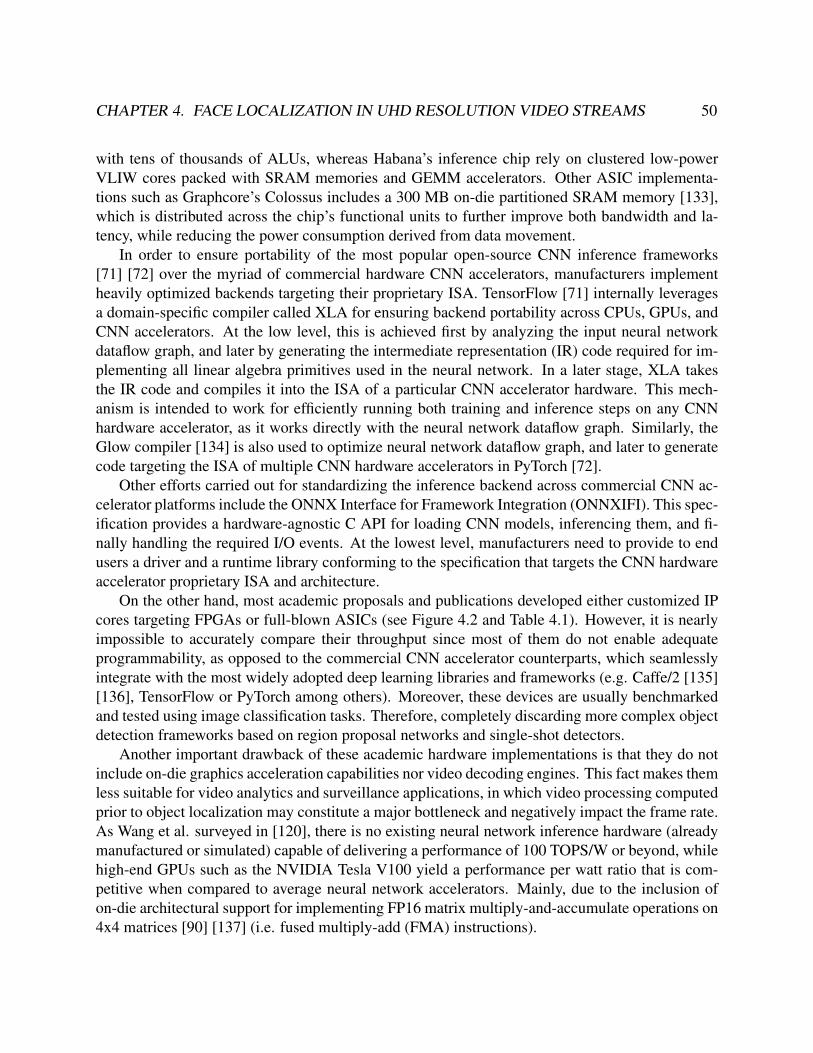
CHAPTER 4. FACE LOCALIZATION IN UHD RESOLUTION VIDEO STREAMS 50
with tens of thousands of ALUs, whereas Habana’s inference chip rely on clustered low-powerVLIW cores packed with SRAM memories and GEMM accelerators. Other ASIC implementa-tions such as Graphcore’s Colossus includes a 300 MB on-die partitioned SRAM memory [133],which is distributed across the chip’s functional units to further improve both bandwidth and la-tency, while reducing the power consumption derived from data movement.
In order to ensure portability of the most popular open-source CNN inference frameworks[71] [72] over the myriad of commercial hardware CNN accelerators, manufacturers implementheavily optimized backends targeting their proprietary ISA. TensorFlow [71] internally leveragesa domain-specific compiler called XLA for ensuring backend portability across CPUs, GPUs, andCNN accelerators. At the low level, this is achieved first by analyzing the input neural networkdataflow graph, and later by generating the intermediate representation (IR) code required for im-plementing all linear algebra primitives used in the neural network. In a later stage, XLA takesthe IR code and compiles it into the ISA of a particular CNN accelerator hardware. This mech-anism is intended to work for efficiently running both training and inference steps on any CNNhardware accelerator, as it works directly with the neural network dataflow graph. Similarly, theGlow compiler [134] is also used to optimize neural network dataflow graph, and later to generatecode targeting the ISA of multiple CNN hardware accelerators in PyTorch [72].
Other efforts carried out for standardizing the inference backend across commercial CNN ac-celerator platforms include the ONNX Interface for Framework Integration (ONNXIFI). This spec-ification provides a hardware-agnostic C API for loading CNN models, inferencing them, and fi-nally handling the required I/O events. At the lowest level, manufacturers need to provide to endusers a driver and a runtime library conforming to the specification that targets the CNN hardwareaccelerator proprietary ISA and architecture.
On the other hand, most academic proposals and publications developed either customized IPcores targeting FPGAs or full-blown ASICs (see Figure 4.2 and Table 4.1). However, it is nearlyimpossible to accurately compare their throughput since most of them do not enable adequateprogrammability, as opposed to the commercial CNN accelerator counterparts, which seamlesslyintegrate with the most widely adopted deep learning libraries and frameworks (e.g. Caffe/2 [135][136], TensorFlow or PyTorch among others). Moreover, these devices are usually benchmarkedand tested using image classification tasks. Therefore, completely discarding more complex objectdetection frameworks based on region proposal networks and single-shot detectors.
Another important drawback of these academic hardware implementations is that they do notinclude on-die graphics acceleration capabilities nor video decoding engines. This fact makes themless suitable for video analytics and surveillance applications, in which video processing computedprior to object localization may constitute a major bottleneck and negatively impact the frame rate.As Wang et al. surveyed in [120], there is no existing neural network inference hardware (alreadymanufactured or simulated) capable of delivering a performance of 100 TOPS/W or beyond, whilehigh-end GPUs such as the NVIDIA Tesla V100 yield a performance per watt ratio that is com-petitive when compared to average neural network accelerators. Mainly, due to the inclusion ofon-die architectural support for implementing FP16 matrix multiply-and-accumulate operations on4x4 matrices [90] [137] (i.e. fused multiply-add (FMA) instructions).
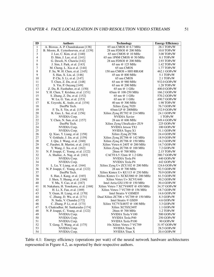
CHAPTER 4. FACE LOCALIZATION IN UHD RESOLUTION VIDEO STREAMS 51
ID Authors Technology Energy Efficiency1 A. Biswas, A. P. Chandrakasan [138] 65 nm CMOS @ 6.7 MHz 28.1 TOPs/W2 B. Moons, R. Uytterhoeven, et al. [139] 28 nm FDSOI @ 200 MHz 10.0 TOPs/W3 J. Lee, C. Kim, et al. [140] 65 nm CMOS @ 10 MHz 3.08 TOPs/W4 D. Shin, J. Lee, et al. [141] 65 nm 1P8M CMOS @ 50 MHz 8.1 TOPs/W5 G. Desoli, N. Chawla [142] 28 nm FDSOI @ 200 MHz 2.93 TOPs/W6 J. Sim, J. Park, et al. [143] 65 nm @ 125 MHz 1.42 TOPs/W7 M. Cheng, L. Xia et al. [144] 65 nm CMOS 1.77 TOPs/W8 F. Su, W. H. Chen, et al. [145] 150 nm CMOS + HfO RRAM 462.1 GOPs/W9 S. Han, X. Liu, al. [146] 45 nm @ 800 MHz 5.1 TOPs/W10 P. Chi, S. Li, et al. [147] 65 nm CMOS 2.1 TOPs/W11 T. Chen, Z. Du, et al. [148] 65 nm @ 980 MHz 932.0 GOPs/W12 S. Yin, P. Ouyang [149] 65 nm @ 200 MHz 1.28 TOPs/W13 Z. Du, R. Fasthuber, et al. [150] 65 nm @ 1 GHz 400.0 GOPs/W14 Y. H. Chen, T. Krishna, et al. [151] 65nm @ 100-250 MHz 166.2 GOPs/W15 S. Zhang, Z. Du, et al. [152] 65 nm @ 1 GHz 570.2 GOPs/W16 W. Lu, G. Yan, et al. [153] 65 nm @ 1 GHz 490.7 GOPs/W17 K. Ueyoshi, K. Ando, et al. [154] 40 nm @ 300 MHz 1.98 TOPs/W18 DeePhi Tech. Xilinx Zynq 7020 76.7 GOPs/W19 F. Tu, S. Yin, et al. [155] 65nm LP @ 200MHz 152.9 GOPs/W20 K. Guo, L. Sui, et al. [156] Xilinx Zynq ZC702 @ 214 MHz 24.1 GOPs/W21 NVIDIA Corp. NVIDIA Xavier 1 TOPs/W22 Y. Chen, N. Sun, et al. [157] 28 nm @ 606 MHz 349.4 GOPs/W23 DeePhi Tech. Xilinx Zynq UltraScale+ ZU9 225 GOPs/W24 NVIDIA Corp. NVIDIA Jetson TX1 100 GOPs/W25 NVIDIA Corp. NVIDIA Tegra X1 31.1 GOPs/W26 Q. Xiao, Y. Liang, et al. [158] Xilinx Zynq ZC706 24.4 GOPs/W27 V. Gokhale, J. Jin, et al. [159] Xilinx Zynq ZC706 @ 142 MHz 18.9 GOPs/W28 J. Qiu, J. Wang, et al. [160] Xilinx Zynq ZC706 @ 150 MHz 14.2 GOPs/W29 C. Farabet, B. Martini, et al. [161] Xilinx Virtex-6 240T @ 200 MHz 14.7 GOPs/W30 Y. Wang, J. Xu, et al. [162] Xilinx Zynq ZC706 @ 100 MHz 7.2 GOPs/W31 N. P. Jouppi, C. Young, et al. [122] 28nm @ 700 MHz 2.15 TOPs/W32 A. Shafiee, A. Nag, et al. [163] CACTI 6.5 32nm @ 1.2 GHz 380.7 GOPs/W33 NVIDIA Corp. NVIDIA Tesla P4 440 GOPs/W34 NVIDIA Corp. NVIDIA Tesla P4 442 GOPs/W35 L. Lu, Y. Liang, et al. [164] Xilinx Zynq U+ ZCU102 @ 200 MHz 124.6 GOPs/W36 N. P. Jouppi, C. Young, et al. [122] 28 nm @ 700 MHz 92.5 GOPs/W37 DeePhi Tech. Xilinx Kintex U+ KU115 @ 250 MHz 70.9 GOPs/W38 S. Han, J. Kang, et al. [165] Xilinx Kintex U+ XCKU060 @ 200 MHz 61.5 GOPs/W39 J. Shen, Y. Huang, et al. [166] Xilinx Virtex U+ XCVU440 30.2 GOPs/W40 Y. Ma, Y. Cao, et al. [167] Intel Arria GX1150 @ 150 MHz 30.4 GOPs/W41 H. Nakahara, H. Yonekawa, et al. [168] Xilinx Virtex-7 XC7V690T @ 450 MHz 34.37 GOPs/W42 H. Li, X. Fan, et al. [169] Xilinx Virtex-7 VC709 @ 156 MHz 18.7 GOPs/W43 Y. Guan, H. Liang, et al. [170] Intel Stratix-V GSMD5 14.6 GOPs/W44 C. Zhang, D. Wu, et al. [171] Dual Xilinx ZC706 + VC709 @ 150 MHz 8.3 GOPs/W45 N. Suda, V. Chandra [172] Intel Stratix-V GSD9 4.6 GOPs/W46 C. Zhang, P. Li, et al. [173] Xilinx VC7VX485T @ 100 MHz 3.3 GOPs/W47 S. Chakradhar, M. Sankaradas [174] Xilinx XC5SX240T 1.1 GOPs/W48 N. P. Jouppi, C. Young, et al. [122] 28nm @ 700 MHz 1.2 TOPs/W49 NVIDIA Corp. NVIDIA Tesla V100 500 GOPs/W50 NVIDIA Corp. NVIDIA Tesla P40 250 GOPs/W51 NVIDIA Corp. NVIDIA Tesla P100 90 GOPs/W52 T. Geng, T. Wang, et al. [175] 10x Xilinx Virtex-7 VC709 31.97 GOPs/W53 NVIDIA Corp. NVIDIA Titan X 28.5 GOPs/W54 NVIDIA Corp. NVIDIA Titan X 20.4 GOPs/W
Table 4.1: Energy efficiency (operations per watt) of the neural network hardware architecturesrepresented in Figure 4.2, as reported by their respective authors.

CHAPTER 4. FACE LOCALIZATION IN UHD RESOLUTION VIDEO STREAMS 52
Finally, it should be noted that the TOPS/W metric may become meaningless for drawing fairperformance comparisons between platforms, as each CNN hardware accelerator relies on its ownproprietary instruction set architecture (ISA). Therefore, the total amount of instructions requiredfor implementing CNN backpropagation and forward pass on each platform may vary substantiallyas well. For this reason, multiple actors of the semiconductor industry and academia have agreed todevelop a standardized set of models and datasets for evaluating the execution time and throughputof both CNN training and inference. The MLPerf [176] initiative is a good step forward in thecomparison of CNN latency on a wide range of microarchitectures.
4.2 Boosted Ensembles vs. CNNs: A Latency PerspectiveIn Chapter 3, we proved that by relying on a proper multi-level parallelization pattern and localon-die caching it is possible to complete the evaluation of cascades of boosted ensembles for facedetection in less than 2 milliseconds for 1080p video workloads on GPU platforms. However, thesemethods based on hand-crafted features and integral images are currently phased out, as they weresurpassed by CNNs, which currently are the gold standard for object localization and recognition.On the particular face detection use case, the early discarding properties of ensemble methods mayprove to be still useful in solving the problem of computing in real time face detection over ultra-high definition (UHD) workloads. One possible idea is to exploit the early discard properties ofcascades of boosted ensembles to skip background regions in large video frames, and later analyzesurviving regions and image patches using a state-of-the-art single-shot CNN. We will furtherelaborate the feasibility of this idea later.
From a performance perspective, ensemble methods yield a variable latency, as for a givensliding window, the maximum stage region reached during evaluation characterizes thread surviv-ability within warps on GPU platforms. Luckily, the high rejection rates of the first stages of thecascade ensures that most regions are discarded after computing a few filters, therefore yieldinga very low but variable latency. On the other hand, conventional single-shot CNN face detectorsmust always perform inference of all of its layers for a given input image, and therefore, theyshould yield a near constant latency. In order to properly characterize this behaviour, we compileda dataset of UHD video benchmarks featuring dozens of simultaneous faces at both 4K and 8Kresolutions. The codec properties of the videos selected for experimentation are summarized be-low in Table 4.2. Moreover, an overview of the facial workloads appearing in the selected 4K/8Kvideos are shown in Figure 4.3.
Dataset Duration Codec Resolution Frame Rate Bitrategangnam.mp4 7 min. 38 s H.264 3840x2026 24 FPS 18.98 Mbpsshibuya.mp4 6 min. 2 s H.264 3840x2160 30 FPS 23.82 Mbpsforbidden.mp4 1 min. 59 s HEVC 7680x4320 30 FPS 59.73 Mbps
Table 4.2: Codec properties of UHD dataset.
For each one of the selected videos, state-of-the-art CNN-based face detection frameworkswere benchmarked and its implementation code instrumented when running on an Intel Core i7-

CHAPTER 4. FACE LOCALIZATION IN UHD RESOLUTION VIDEO STREAMS 53
Legend Framework Feature Extractor Network Input SizeA Faster R-CNN [55] ResNet-50 1000x600B SSD [57] ResNet-50 300x300C S3FD [116] VGG-16 640x640D R-FCN [56] ResNet-101 1000x600E FPN [112] ResNet-50 300x300F YOLOv3 [58] DarkNet-53 416x416G Cascade R-CNN [177] ResNet-101 1280x800H Mask R-CNN [108] ResNet-101 1280x800
Table 4.3: Benchmarked CNN-based face detection frameworks.
4770 coupled with an NVIDIA Tesla T4. Similarly, a cascade of LBP features was also executedon the same reference platform for illustrating its potentiality for early discarding in large images.As Table 4.3 shows, selected CNN-based frameworks mostly rely on the widely used ResNet [52]and VGG [51] networks as feature extractors, and implement different region proposal techniquesin order to reduce the burden of computations. In contrast, Table 4.4 shows the properties of theselected face detection framework based on a cascade of boosted ensembles, which was trainedusing the WaldBoost [70] algorithm and organized into 1000 stages, each one containing a singleLBP feature. The underlying GPU implementation of this framework follows the parallelizationpattern described in [69], and splits the evaluation of the cascade into four CUDA kernels usingthread rearrangement techniques to minimize the impact of thread divergence.
(a) gangnam.mp4 (b) shibuya.mp4
(c) forbidden.mp4
Figure 4.3: Appearance of selected 4K and 8K videos.
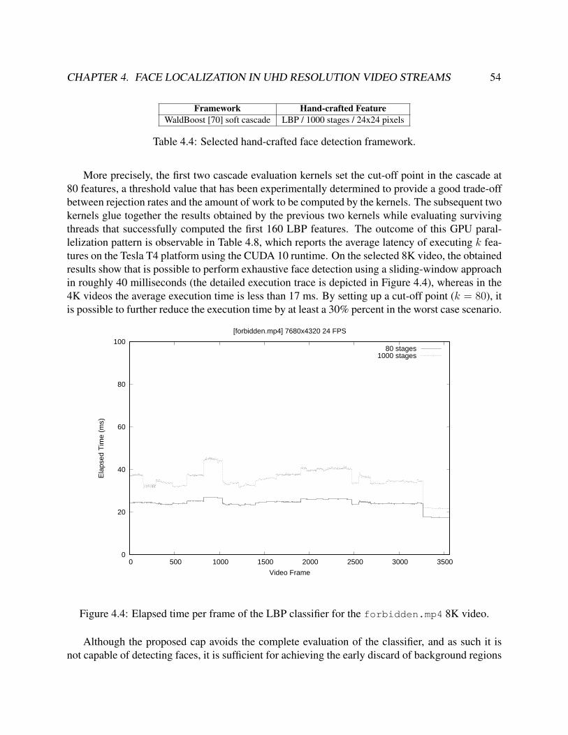
CHAPTER 4. FACE LOCALIZATION IN UHD RESOLUTION VIDEO STREAMS 54
Framework Hand-crafted FeatureWaldBoost [70] soft cascade LBP / 1000 stages / 24x24 pixels
Table 4.4: Selected hand-crafted face detection framework.
More precisely, the first two cascade evaluation kernels set the cut-off point in the cascade at80 features, a threshold value that has been experimentally determined to provide a good trade-offbetween rejection rates and the amount of work to be computed by the kernels. The subsequent twokernels glue together the results obtained by the previous two kernels while evaluating survivingthreads that successfully computed the first 160 LBP features. The outcome of this GPU paral-lelization pattern is observable in Table 4.8, which reports the average latency of executing k fea-tures on the Tesla T4 platform using the CUDA 10 runtime. On the selected 8K video, the obtainedresults show that is possible to perform exhaustive face detection using a sliding-window approachin roughly 40 milliseconds (the detailed execution trace is depicted in Figure 4.4), whereas in the4K videos the average execution time is less than 17 ms. By setting up a cut-off point (k = 80), itis possible to further reduce the execution time by at least a 30% percent in the worst case scenario.
0
20
40
60
80
100
0 500 1000 1500 2000 2500 3000 3500
Ela
psed
Tim
e (m
s)
Video Frame
[forbidden.mp4] 7680x4320 24 FPS
80 stages1000 stages
Figure 4.4: Elapsed time per frame of the LBP classifier for the forbidden.mp4 8K video.
Although the proposed cap avoids the complete evaluation of the classifier, and as such it isnot capable of detecting faces, it is sufficient for achieving the early discard of background regions

CHAPTER 4. FACE LOCALIZATION IN UHD RESOLUTION VIDEO STREAMS 55
Dataset [Tedc] Average Execution Time (ms)k = 80 k = 1000
gangnam.mp4 6.04 10.26shibuya.mp4 6.97 16.96
forbidden.mp4 24.43 34.84
Table 4.5: Execution time of k stages of the LBP classifier for the selected workloads.
Dataset [Tcnn] Average Inference Time (ms)A B C D E F G H
gangnam.mp4 107.30 7.63 28.42 75.55 163.64 23.11 97.29 143.55shibuya.mp4 118.44 7.83 32.06 77.41 164.17 22.88 97.16 158.46
forbidden.mp4 124.89 7.79 29.38 78.69 166.78 24.42 98.63 143.83
Table 4.6: Inference time of benchmarked CNN-based frameworks for the selected workloads.
not containing faces. On the other hand, as Figure 4.5 illustrates, a typical CNN-based classifiertends to yield a near constant latency on a per frame basis. We found that the slightly positiveslope depicted in this graph was related to the progressive increase in GPU temperature due to theselection of the adaptive power mode of the device. Table 4.6 shows the average inference timeper frame for the selected CNN-based classifiers when processing UHD video workloads. Theselatter preliminary experiments were conducted on the same GPU platform as the LBP classifier,but they did not involve in-house low-level CUDA kernels developed by us. They relied instead onNVIDIA’s cuDNN 7.6 library and PyTorch 1.4.0.
It should be noted, though, that for this particular experiment video frames were downscaledto the input size of each single-shot CNN, and as opposed to the LBP classifier, it did not per-form an exhaustive brute force evaluation of images through a sliding window. Referring againto Figure 4.5, this means 8K frames were dynamically resized to the input dimensions of the se-lected YOLOv3 model: 416x416. As a result of this huge downscale process, accuracy may beseverely hindered. Due to the lack of annotated UHD video datasets containing faces, it was notpossible for us to rigorously quantify the error. In that sense, Ruzicka et al. [178] reported roughlya 20% improvement in average precision (AP) when performing crop and tiling on UHD imagesbefore inferencing YOLOv2 over the PEViD-UHD pedestrian data set [179], rather than naivelydownscaling them to the input size of the neural network.
However, the feasibility of relying on an hybrid approach combining a capped classifier basedon hand-crafted features followed by a CNN still remains valid. In particular, by summing up theexecution time of both classifiers (Tedc + Tcnn) on the Tesla T4 platform, the obtained preliminaryresults showed that it was possible to achieve near real-time throughput. Unfortunately, only afew of the selected frameworks (SSD, S3FD, and YOLOv3) were lightweight enough for thispurpose. Methods performing instance segmentation such as Cascade R-CNN and Mask R-CNNwere among the slowest, while others conducting simple object detection (Faster R-CNN, R-FCN,and FPN) were not fast enough for meeting our timing constraints.
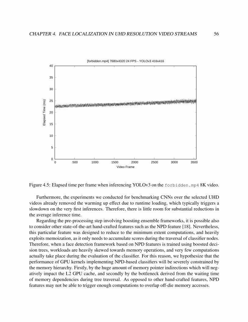
CHAPTER 4. FACE LOCALIZATION IN UHD RESOLUTION VIDEO STREAMS 56
0
5
10
15
20
25
30
35
40
0 500 1000 1500 2000 2500 3000 3500
Ela
psed
Tim
e (m
s)
Video Frame
[forbidden.mp4] 7680x4320 24 FPS - YOLOv3 416x416
Figure 4.5: Elapsed time per frame when inferencing YOLOv3 on the forbidden.mp4 8K video.
Furthermore, the experiments we conducted for benchmarking CNNs over the selected UHDvideos already removed the warming up effect due to runtime loading, which typically triggers aslowdown on the very first inferences. Therefore, there is little room for substantial reductions inthe average inference time.
Regarding the pre-processing step involving boosting ensemble frameworks, it is possible alsoto consider other state-of-the-art hand-crafted features such as the NPD feature [18]. Nevertheless,this particular feature was designed to reduce to the minimum extent computations, and heavilyexploits memoization, as it only needs to accumulate scores during the traversal of classifier nodes.Therefore, when a face detection framework based on NPD features is trained using boosted deci-sion trees, workloads are heavily skewed towards memory operations, and very few computationsactually take place during the evaluation of the classifier. For this reason, we hypothesize that theperformance of GPU kernels implementing NPD-based classifiers will be severely constrained bythe memory hierarchy. Firstly, by the huge amount of memory pointer indirections which will neg-atively impact the L2 GPU cache, and secondly by the bottleneck derived from the waiting timeof memory dependencies during tree traversal. As opposed to other hand-crafted features, NPDfeatures may not be able to trigger enough computations to overlap off-die memory accesses.
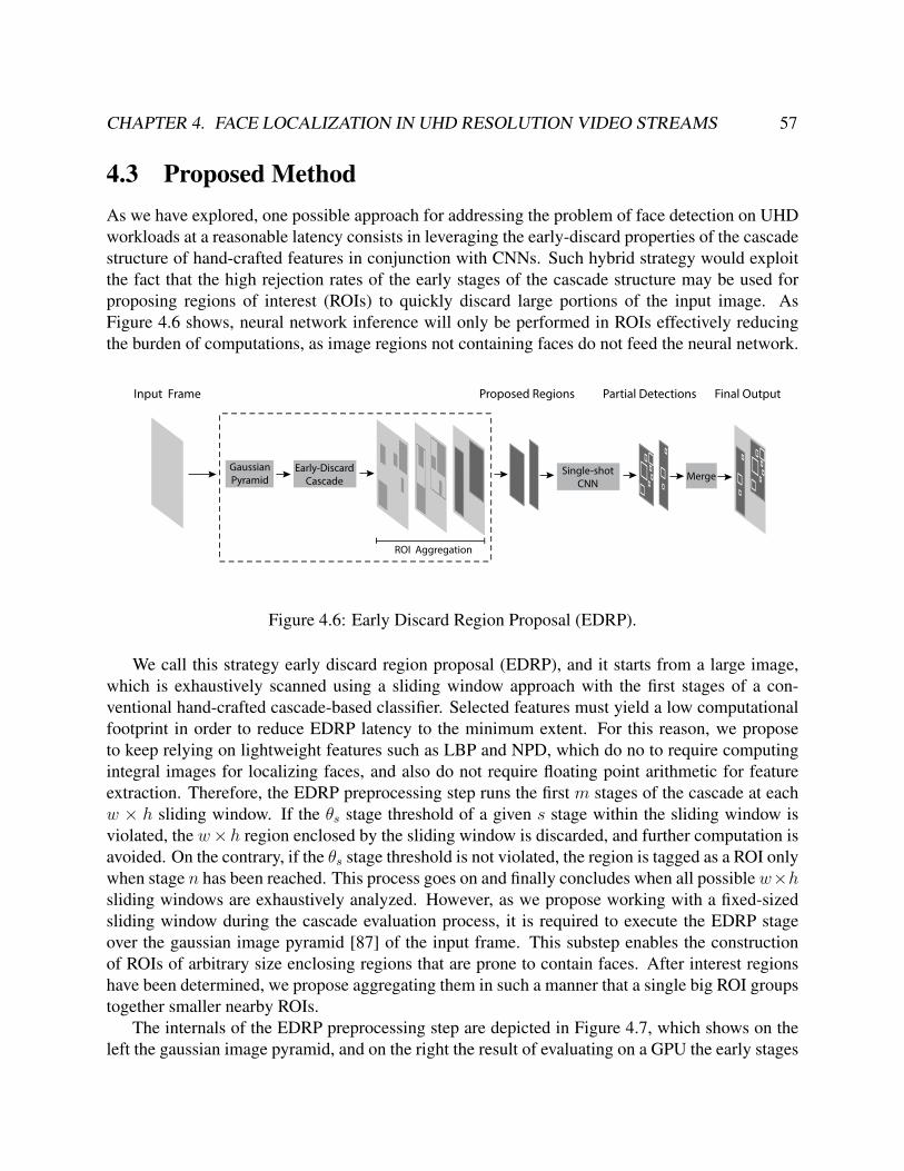
CHAPTER 4. FACE LOCALIZATION IN UHD RESOLUTION VIDEO STREAMS 57
4.3 Proposed MethodAs we have explored, one possible approach for addressing the problem of face detection on UHDworkloads at a reasonable latency consists in leveraging the early-discard properties of the cascadestructure of hand-crafted features in conjunction with CNNs. Such hybrid strategy would exploitthe fact that the high rejection rates of the early stages of the cascade structure may be used forproposing regions of interest (ROIs) to quickly discard large portions of the input image. AsFigure 4.6 shows, neural network inference will only be performed in ROIs effectively reducingthe burden of computations, as image regions not containing faces do not feed the neural network.
Early-DiscardCascade
Input Frame
Single-shotCNN
Proposed Regions
Merge
Partial Detections Final Output
GaussianPyramid
ROI Aggregation
Figure 4.6: Early Discard Region Proposal (EDRP).
We call this strategy early discard region proposal (EDRP), and it starts from a large image,which is exhaustively scanned using a sliding window approach with the first stages of a con-ventional hand-crafted cascade-based classifier. Selected features must yield a low computationalfootprint in order to reduce EDRP latency to the minimum extent. For this reason, we proposeto keep relying on lightweight features such as LBP and NPD, which do no to require computingintegral images for localizing faces, and also do not require floating point arithmetic for featureextraction. Therefore, the EDRP preprocessing step runs the first m stages of the cascade at eachw × h sliding window. If the θs stage threshold of a given s stage within the sliding window isviolated, the w×h region enclosed by the sliding window is discarded, and further computation isavoided. On the contrary, if the θs stage threshold is not violated, the region is tagged as a ROI onlywhen stage n has been reached. This process goes on and finally concludes when all possible w×hsliding windows are exhaustively analyzed. However, as we propose working with a fixed-sizedsliding window during the cascade evaluation process, it is required to execute the EDRP stageover the gaussian image pyramid [87] of the input frame. This substep enables the constructionof ROIs of arbitrary size enclosing regions that are prone to contain faces. After interest regionshave been determined, we propose aggregating them in such a manner that a single big ROI groupstogether smaller nearby ROIs.
The internals of the EDRP preprocessing step are depicted in Figure 4.7, which shows on theleft the gaussian image pyramid, and on the right the result of evaluating on a GPU the early stages

CHAPTER 4. FACE LOCALIZATION IN UHD RESOLUTION VIDEO STREAMS 58
0 2 4 6 8 10 12 14 16 18 20Stage
Figure 4.7: Discarded regions in EDRP (right) derived from an NPD face classifier (20 stages).
(m = 20) of a 24x24 pixel NPD face classifier [18]. The NPD classifier quickly discards back-ground regions, while surviving regions (m > 20) that are likely to contain faces are cropped andforwarded to the single-shot CNN framework in order to complete the accurate facial detection pro-cess. As this framework is designed to work with very large input frames and relies on a gaussianimage pyramid for enabling multi-scale face detection, EDRP potentially increases the chances ofdetecting small faces. Moreover, it also offers opportunities for enabling coarse grain parallelismwhen inferencing the cropped regions either on the same GPU in which EDRP is computed or onan additional neural network accelerator.
The pseudocode of the proposed framework is summarized in Algorithm 3. The EDRP pro-cess requires as an input the I image, a boosted cascade F of T stages, and the m cut-off point.Internally, both the gaussian pyramid kernel and the cascade evaluation kernel are expected to beexecuted on the GPU platform. The cascade evaluation kernel returns an S matrix of integers ofsize W ′ × H ′ (corresponding to the dimensions of the gaussian pyramid), in which for all s ∈ Seach integer encodes the maximum stage of the cascade reached until meeting the m cut-off point.

CHAPTER 4. FACE LOCALIZATION IN UHD RESOLUTION VIDEO STREAMS 59
Figure 4.8: Estimation of ROIs (right) after applying CLIQUE clustering to the NPD classifierresponses (middle) obtained from the gaussian pyramid corresponding to an 8K frame (left).
In contrast to the two previous kernels, the ROI aggregation kernel should exhibit a low com-putational footprint in order to be executed on a multicore CPU in just a few milliseconds. Wedecided to discard the design of a GPU kernel for solving the aggregation because unless there areseveral millions of points to be aggregated, the launch overhead of a small GPU kernel with a fewthousands of points is typically uncompetitive when compared to a CPU implementing the under-lying clustering process [180]. After the ROI aggregation is computed, Algorithm 3 proceeds withthe CNN inference of each r ∈ R region in parallel over the GPU or the neural network acceleratorresources. Finally, the EDRP process returns the D set of detections containing the union of thecoordinates of all detected faces in each region.
With regard to the construction and merging of ROIs, we initially proposed to rely on a grid-based clustering approach, in which the data space is partitioned using a finite number of cellsconstituting a grid structure, and later generate clusters directly from the cells. By following thisstrategy, it is possible to cluster the surrounding regions close to the data points enclosed by thecells, thus effectively performing the merging of ROIs. In our scenario, data points are simplythe mapped (x, y) coordinates of the response of the w × h-pixel NPD classifier, and locationswith high cell point densities represent ROIs. Therefore, the two dimensional clustering processvis-a-vis each cell within the grid effectively performs the desired ROI aggregation.
Formally, a proper ROI aggregation strategy should rely on this automatic subspace clusteringtechnique. A method that efficiently implements this process is the CLIQUE algorithm proposed

CHAPTER 4. FACE LOCALIZATION IN UHD RESOLUTION VIDEO STREAMS 60
Algorithm 3: EDRP-based Face DetectionData: Matrix I of size W ×H , Matrix F of size T , Integer mbegin
I ′ ← GAUSSIANPYRAMIDKERNEL(I)S ← CASCADECLASSIFIERKERNEL(I ′, F,m)R← AGGREGATEROI(I ′, S)for each r in R parallel do
D′ ← INFERENCECNNMODEL(r)D′′ ← D′′ ∪D′
endD ← MERGEDETECTIONS(D′′)
end
by Agrawal et al. [181] (see Figure 4.8). The main benefits behind such algorihm is that it doesnot require to provide beforehand any assumption on the amount of clusters, and its grid-basedstrategy is designed for handling large data sets. In our use case, the time complexity of clusteringis significantly reduced, as the number of cells within the grid is usually smaller than the numberof data points (n), the grid structure is static, and input data belongs to the R2 space (k = 2).
Unfortunately, as we are constrained by the real-time nature of face detection, it might not bepossible to meet the tight deadline. In order to prove this hypothesis, we benchmarked an optimizedC++ implementation of CLIQUE [182] together with other well-known grid-based clustering al-gorithms and the Lloyd’s version of k-means [183] on an Intel Core i7-4770 CPU clocked at 3.40GHz. These clustering algorithms were executed using as input data points the output response ofrunning the first 20 stages of a 24x24 pixel NPD face classifier over the 8K video frames of theforbidden.mp4 dataset. The obtained results of this preliminary analysis are shown in Table 4.7.
AggregateROI Worst-Case Time Complexity Latency (ms)CLIQUE [181] O(nk + ck) 170
HDBSCAN [184] O(n2) 152DBSCAN [185] O(n2) 105k-means [183] O(2nk2Ω(
√n)) 31
Table 4.7: Average latency per frame during ROI aggregation on forbidden.mp4 video.
As we previously estimated, the sum of the execution of the early-discard cascade (Tedc) andCNN inference (Tcnn) should be in line with the 40 ms of the real-time processing deadline. There-fore, the obtained results completely invalidate the usage of grid-based clustering algorithms. Evenk-means is not fast enough for enabling the real-time execution of the complete EDRP pipeline.As a result of this, another strategy relying on simpler and lightweight heuristics must be followedfor implementing ROI aggregation.
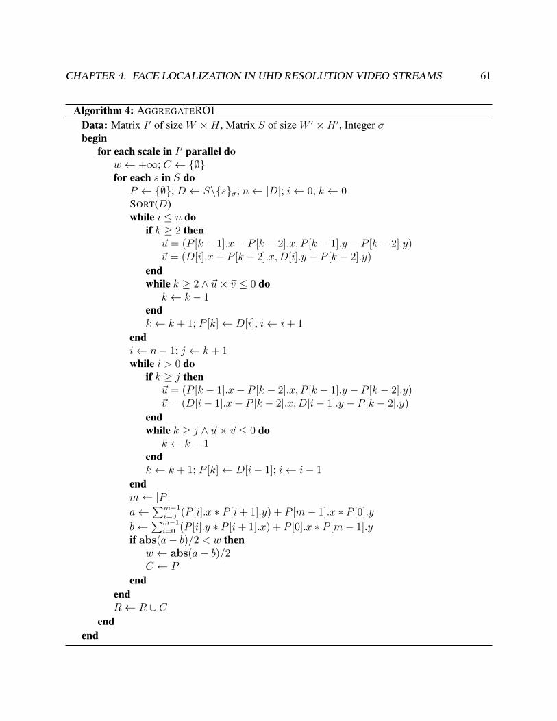
CHAPTER 4. FACE LOCALIZATION IN UHD RESOLUTION VIDEO STREAMS 61
Algorithm 4: AGGREGATEROIData: Matrix I ′ of size W ×H , Matrix S of size W ′ ×H ′, Integer σbegin
for each scale in I ′ parallel dow ← +∞; C ← ∅for each s in S do
P ← ∅; D ← S\sσ; n← |D|; i← 0; k ← 0SORT(D)while i ≤ n do
if k ≥ 2 then~u = (P [k − 1].x− P [k − 2].x, P [k − 1].y − P [k − 2].y)~v = (D[i].x− P [k − 2].x,D[i].y − P [k − 2].y)
endwhile k ≥ 2 ∧ ~u× ~v ≤ 0 do
k ← k − 1endk ← k + 1; P [k]← D[i]; i← i+ 1
endi← n− 1; j ← k + 1while i > 0 do
if k ≥ j then~u = (P [k − 1].x− P [k − 2].x, P [k − 1].y − P [k − 2].y)~v = (D[i− 1].x− P [k − 2].x,D[i− 1].y − P [k − 2].y)
endwhile k ≥ j ∧ ~u× ~v ≤ 0 do
k ← k − 1endk ← k + 1; P [k]← D[i− 1]; i← i− 1
endm← |P |a←
∑m−1i=0 (P [i].x ∗ P [i+ 1].y) + P [m− 1].x ∗ P [0].y
b←∑m−1
i=0 (P [i].y ∗ P [i+ 1].x) + P [0].x ∗ P [m− 1].yif abs(a− b)/2 < w then
w ← abs(a− b)/2C ← P
endendR← R ∪ C
endend
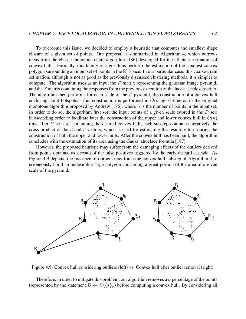
CHAPTER 4. FACE LOCALIZATION IN UHD RESOLUTION VIDEO STREAMS 62
To overcome this issue, we decided to employ a heuristic that computes the smallest shapeclosure of a given set of points. Our proposal is summarized in Algorithm 4, which borrowsideas from the classic monotone chain algorithm [186] developed for the efficient estimation ofconvex hulls. Formally, this family of algorithms perform the estimation of the smallest convexpolygon surrounding an input set of points in the R2 space. In our particular case, this coarse-grainestimation, although is not as good as the previously discussed clustering methods, it is simpler tocompute. The algorithm uses as an input the I ′ matrix representing the gaussian image pyramid,and the S matrix containing the responses from the previous execution of the face cascade classifier.The algorithm then performs for each scale of the I ′ pyramid, the construction of a convex hullenclosing point hotspots. This construction is performed in O(n log n) time as in the originalmonotone algorithm proposed by Andrew [186], where n is the number of points in the input set.In order to do so, the algorithm first sort the input points of a given scale (stored in the D set)in ascending order to facilitate later the construction of the upper and lower convex hull in O(n)time. Let P be a set containing the desired convex hull, each substep computes iteratively thecross-product of the ~u and ~v vectors, which is used for estimating the resulting turn during theconstruction of both the upper and lower hulls. After the convex hull has been built, the algorithmconcludes with the estimation of its area using the Gauss’ shoelace formula [187].
However, the proposed heuristic may suffer from the damaging effects of the outliers derivedfrom points obtained as a result of the false positives triggered by the early-discard cascade. AsFigure 4.9 depicts, the presence of outliers may force the convex hull substep of Algorithm 4 toerroneously build an undesirable large polygon consuming a great portion of the area of a givenscale of the pyramid.
P
P
P
PP
P
P
P
P
P
P
PP
P
P
0
1
2
n-13
4
5 6
0
1
2
n-13
5 6
Figure 4.9: Convex hull considering outliers (left) vs. Convex hull after outlier removal (right).
Therefore, in order to mitigate this problem, our algorithm removes a σ percentage of the points(represented by the statement D ← S\sσ) before computing a convex hull. By considering all

CHAPTER 4. FACE LOCALIZATION IN UHD RESOLUTION VIDEO STREAMS 63
s ∈ S points, and removing the σ percentage at each iteration of the loop, the convex hull enclosingS with the minimal w area among all possible combinations is effectively selected. Finally, theobtained set of points constituting the selected convex hull (represented by C) is added to the Rlist to be returned by the AGGREGATEROI function.
An example of the execution of the proposed heuristic over the forbidden.mp4 video datasetafter having computed the gaussian image pyramid is shown in Figure 4.10 included below. Con-structed convex hulls are highlighted in slightly gray color. It should be noted though that forseveral smaller scales, the convex hull construction did not take place, as the execution of theprevious face classifier always triggered early rejections for all sliding windows.
Figure 4.10: Output of the AGGREGATEROI heuristic.
After this process concludes, Algorithm 3 estimates the boxes enclosing the computed convexhulls in order to crop ROIs and feed all subsequent CNN inferences (INFERENCECNNMODEL),which are scheduled and executed in parallel. Finally, EDRP concludes by merging the obtaineddetections, and by applying a coordinate transformation to effectively map them from the gaussianpyramid to the original input video frame.
The proposed algorithm and heuristics, although simple to implement when compared to ad-vanced clustering methods, are targeted to real time workloads and exploit naive coarse grain paral-lelism, as each region corresponding to a different image pyramid scale is independently scheduled.Moreover, further parallelization is still possible through vectorization during the estimation of theconvex hull areas.
CHAPTER 4. FACE LOCALIZATION IN UHD RESOLUTION VIDEO STREAMS 64
4.4 Experimental SetupTo evaluate the computational performance of EDRP, we relied on the LBP GPU face classifierpreviously presented in Table 4.4. Since we were not able to find in the literature existing worksreporting the performance of NPD features on GPU architectures, we designed and wrote fromscratch a CUDA kernel to evaluate them. This latter classifier consisted in a quadratic boostedtree of 1226 stages, as in the original work of Liao et al [18]. Under this classifier architecture,each inner node encoded and evaluated a given NPD feature, while terminal nodes simply returnedscores computed during training. In our GPU implementation, pointers and tree nodes (includingthresholds, NPD coordinates, and scores) were stored as textures and recovered by texture fetcheswithin the kernel. The parallelization pattern implemented a 24x24 sliding window approach, inwhich a given (x, y) thread performed tree traversal, accumulated the obtained scores, and finallystored them together with the maximum stage reached in the global memory address space. Weomit including in this section the pseudocode of our CUDA GPU implementation, as it is similarin nature to the one described in Chapter 3. Nevertheless, as opposed to the previously presentedimplementation, our NPD evaluation kernel did not rely on the shared memory for bringing nearbyimage pixels on die. The NPD kernel relied instead on tex2D() instructions, which properlyleveraged the GPU texture cache when accessing adjacent pixels.
The rationale behind selecting LBP and NPD features for the early discard substep of EDRPwas to study the impact on GPU performance of compute bound and memory bound features,while determining which one were most suitable for handling UHD workloads in real time.
The GAUSSIANPYRAMIDKERNEL was also implemented as a GPU kernel using the spatialarrangement shown in Figures 4.7, 4.8, and 4.10. For performing the downscaling we dependedon textures indexed by floating point coordinates using 1
4√2as a scaling factor. As an example,
for a conventional input 8K video frame (7680x4320), the resulting pyramid had a resolution of7680x15736 pixels totalling 32 different scales.
On the other hand, the AGGREGATEROI function was derived mainly from a C++ CPU imple-mentation of Algorithm 4, in which we considered σ = 10% during the point removal substep. TheINFERENCECNNMODEL function extensively used the PyTorch C++ API, while the MERGEDE-TECTIONS step was implemented simply by computing boxes enclosing the obtained convex hulls.All experiments were executed on the same hardware in which we conducted our preliminaryanalysis: a multicore Intel Core i7-4770 clocked at 3.40 GHz and an NVIDIA Tesla T4 runningon top of the Linux Kernel 4.15. The host CPU source code was compiled using -O3 optimiza-tion level, whereas GPU kernels targeted the sm 75 architecture. CNN inference was acceleratedusing cuDNN 7.6. To conclude, for obtaining timing measurements, we called multiple times thehigh resolution clock::now() method shipped in std::chrono C++ library.
As UHD data sets, we selected the H.264 videos already presented in Section 4.2. The videoprocessing pipeline closely resembled the one presented in Figure 3.1 in Chapter 3. However, it didnot include the stage related to integral image computation, as the selected LBP and NPD featuresdirectly work with the luminance component of a given video frame. Finally, video decoding wasaccelerated at the low-level with fixed-function hardware by means of the NVDEC library [84],which enabled 8K HEVC/H.265 decoding at high throughput on the NVIDIA Tesla T4 GPU.

CHAPTER 4. FACE LOCALIZATION IN UHD RESOLUTION VIDEO STREAMS 65
Dataset Average Execution Time (ms)k = 20 k = 100 k = 1226
gangnam.mp4 105.88 176.31 189.26shibuya.mp4 156.50 272.98 302.10forbidden.mp4 229.58 316.27 331.68
Table 4.8: GPU execution time of k stages of the NPD classifier for the selected workloads.
4.5 ResultsIn order to determine whether the cascade evaluation kernel of the NPD feature was suitable forGPU architectures, we profiled its execution over the videos presented in Table 4.2. The aim of thisexperiment was to determine if, as we hypothesized, the NPD evaluation kernel was effectivelymemory-bound, and if so, to figure out whether the execution time per frame of this particularkernel was lower than the previously discussed LBP feature (Table 4.8).
Unfortunately, the execution time of the NPD evaluation kernel on the Tesla T4 proved theunfeasibility of relying on such feature for performing early discard in UHD video streams. Evenwhen running very few stages of the classifier (k = 20), the obtained latency was between 2.64 and5.73 times higher than the 40 ms deadline required for real-time processing, as it is summarizedin Table 4.8. With the aim of finding out the reason why the execution time of this kernel wasso high, we sampled the assembly instructions of all active warps using the NVIDIA’s NsightCompute profiler. The sample distribution of stall latencies is depicted in Figure 4.11 below.
Other (13.84%)
Instruction Issued (5.71%)
Memory Dependency (39%)
Instruction Fetch (11.58%)
Execution Dependency (29.87%)
Figure 4.11: Distribution of latencies due to stalls during the NPD kernel execution.

CHAPTER 4. FACE LOCALIZATION IN UHD RESOLUTION VIDEO STREAMS 66
The profile distribution of latencies during kernel execution clearly shows that 68.87% of thestalls were due to the unavailability of input operands during instruction execution (29.87%), or theimpossibility of executing the required load/store operations in the memory hierarchy (39%). Thislatter fact means that memory dependences triggered stalls in the pipeline of the GPU microarchi-tecture when executing kernel instructions. The explanation of this behaviour lies in the quadraticboosted tree structure used in the NPD face classifier. As scores are stored in the terminal nodes oftrees within each stage of the classifier, it is required to perform a significant amount of memoryindirections during tree traversal. As a result of this, very few computations are actually issued forexecution in the ALUs due to the unavailability of operands, and also because a given thread onlyneeds to accumulate the scores of terminal nodes when analyzing a 24x24-pixel sliding window.Also, the hardware texture caches available in the memory hierarchy of the GPU are not able tocope with large sequences of memory indirections. As Figure 4.12 illustrates, kernel performanceis limited by the latency of memory operations, and fine-grained thread-level parallelism over abandwidth-oriented microarchitecture is not the most suitable computational method to address amemory-bound algorithm with an irregular control flow.
xy
Evaluation Window
Block (i,j)
Classifier Cascade Tree NodeMemory Indirections
Figure 4.12: Memory indirections derived from the quadatric boosted tree.
Furthermore, the NPD cascade evaluation kernel yielded a low compute throughput (20% uti-lization of the computational resources and 15% of peak memory bandwidth) clearly indicatingthat it was bounded by the latency of memory operations (Table 4.9). In summary, given theobtained results, it is difficult to obtain additional performance gains through low-level code opti-mization, and the only remaining strategy should focus instead on a large reduction in the size ofthe classifier cascade. Unfortunately, as we showed in Table 4.8, even considering 20 stages, it is

CHAPTER 4. FACE LOCALIZATION IN UHD RESOLUTION VIDEO STREAMS 67
GPU Resources [Tesla T4] Utilization (%)Arithmetic 21
Control Flow 8Memory 9Texture 15
Achieved Occupancy 44.1
Table 4.9: Utilization of the different GPU resources while executing the NPD kernel.
Dataset Average Execution Time (ms)gangnam.mp4 1.54shibuya.mp4 1.21
forbidden.mp4 2.79
Table 4.10: Average execution time per frame of the proposed AGGREGATEROI. The heuristicyields lower execution times than the clustering algorithms presented in Table 4.7
not possible to achieve real time throughput. As a result, there is no particular performance ben-efit to be obtained from training smaller cascades with degraded accuracy. For these reasons, thememory-bound NPD classifier does not meet our performance requirements for early discardingregions in EDRP. Consequently, our initial hypothesis turned out to be true, and compute-boundfeatures not requiring integral images such as LBP represent the only remaining viable option forimplementing our strategy.
On the other hand, the AGGREGATEROI heuristic, which is key for quickly merging and gen-erating ROIs after executing the hand-crafted LBP classifier, proved to be lightweight enough forhandling UHD workloads in real time. As Table 4.10 summarizes, the average execution time perframe of the heuristic was less than 3 ms on the selected multicore CPU platform when processingour UHD datasets. An in-depth analysis of AGGREGATEROI is depicted in Figure 4.13. Thisgraph shows the elapsed time per frame of our heuristic when processing the output of the early-discard LBP (k = 80) substep in EDRP for the 8K forbidden.mp4 dataset. As it was previouslydiscussed, the resulting LBP classifier responses were mainly points in the R2 space, and videoframes featuring large quantities of points were highly correlated with the peak execution time ofthe heuristic. Moreover, these results were consistent with the theoretical computational complex-ity of the algorithm. Also, we experimentally estimated that the AGGREGATEROI heuristic wasbetween 15 and 60 times faster than the clustering methods previously mentioned in Table 4.7.
It could be argued that our heuristic is not robust and may not be able to properly handle outliersin challenging situations, but due to the small time slot available for generating the ROIs, it is theprice to pay for handling UHD workloads in real time. Nevertheless, the presence of outliers isnot catastrophic, as it only produces larger ROIs that are subsequently processed by the underlyingCNN used in EDRP.
To conclude, we measured the computational performance of all the resource-intensive stagesconstituting the EDRP-based face detection engine packed together. In order to do so, we bench-marked the complete framework using SSD, S3FD, and YOLOv3 as the refining CNNs employed

CHAPTER 4. FACE LOCALIZATION IN UHD RESOLUTION VIDEO STREAMS 68
Figure 4.13: Elapsed time per frame of AGGREGATEROI for the forbidden.mp4 8K video.
in the INFERENCECNNMODEL stage over our UHD video datasets. The obtained results are de-picted in Figure 4.14, which aggregates the average execution time in milliseconds of Algorithm 3on a per frame basis. Even though that we extensively optimized EDRP to try to meet the real timedeadline also for 8K resolutions (forbidden.mp4), it was only possible to achieve 21 FPS (nearreal-time performance) when we relied on the CNN-based SSD face detector. For this particularsetup, the average execution time per frame of face detection implementing EDRP was 48 ms for8K resolutions, and roughly 18 ms for 4K resolutions (gangnam.mp4 and shibuya.mp4). How-ever, due to the computational complexity of S3FD and YOLOv3, and even considering that theCNN inference process was optimized at the lowest level using cuDNN and accelerated in hard-ware by means of the tensor cores available on the Tesla T4, the resulting throughput of this lattersetup was too low to handle 8K resolutions in real time. Nevertheless, all tested configurations(SSD, S3FD and YOLOv3) succeeded on handling in real time the selected 4K video datasets.
It is also worth mentioning that the execution time of the image pyramid generation kernelwas constant, as the amount of scales depended on the input resolution. For 4K resolutions, thisparticular kernel took 3 ms, whereas for the 8K video the execution time was 13 ms. This re-markable difference was due to the high number of scales and the resolution selected for the image

CHAPTER 4. FACE LOCALIZATION IN UHD RESOLUTION VIDEO STREAMS 69
gangnam.mp4
shibuya.mp4
forbidden.mp4
EDRP / Face Detection
Figure 4.14: Average execution time per frame of the proposed EDRP-based face detection engineover the selected UHD video datasets. The dashed line represents the hard deadline not to besurpassed for achieving real time throughput.
pyramid on 8K resolutions (7680x15736). This fact also explains why the execution time of theLBP cascade evaluation kernel when processing the 8K dataset is four times higher than for the 4Kworkloads. In that sense, the image pyramid generation kernel could be further optimized for 8Kresolutions by fine-tuning either the amount of considered scales or the downscaling factor applied.
The process described in Algorithm 3 concludes by calling the MERGEDETECTIONS kernel,which is responsible for gathering and combining the partial detections obtained from each CNN.The execution time of this kernel on the Tesla T4 platform was negligible. A detailed overviewof the low-level GPU parallelization of the non-maximum suppression implementation used in thefinal step of EDRP is presented in Chapter 5.
Finally, the obtained performance results were in line with our initial expectations, and showedthat both the parallelization paradigm and hybrid object localization approach exposed in EDRPrepresent a promising approach for addressing the issue of real-time face detection in ultra-high

CHAPTER 4. FACE LOCALIZATION IN UHD RESOLUTION VIDEO STREAMS 70
definition workloads. Moreover, EDRP offers enough flexibility for simultaneoulsy employingmultiple refining CNN architectures with different input resolutions. Consequently, they couldbe later optimally mapped to the proper ROI generated as a result of the execution of the priorhand-crafted classifier according to their dimensions.
4.6 ConclusionsIn this chapter we have presented a practical approach and a heuristic designed to handle ultra-high definition workloads by combining hand-crafted features with state-of-the-art CNN-basedface detection frameworks. Our analysis show that is a good step towards the goal of achievinga full-blown parallel pipeline capable of processing in real time workloads at 8K resolutions andbeyond. Furthermore, emerging heterogeneous architectures such as NVIDIA’s Xavier [7] com-bining a CUDA-enabled GPU with neural network accelerator hardware [131] on a single die maybenefit from EDRP. For instance, it could be theoretically possible to concurrently exploit bothcomputational units while processing several video streams in parallel.
On the other hand, we found that only compute-bound hand-crafted features are suitable forGPU-like microarchitectures during the early-discard stage of the EDRP framework. State-of-the-art features fine-tuned for face detection exploiting memoization (i.e. NPD) are memory-bound,as they were designed for latency-oriented CPU architectures. When combined with a boosted treeclassifier and executed on a GPU, they are not capable of issuing enough amounts of computationalwork to keep the underlying ALUs busy due to the stalls triggered by the large sequences ofmemory indirections.
Future work may involve studying other heuristics involving more robust approaches for effi-ciently handling outliers in challenging scenarios during the ROI aggregation process.

71
Chapter 5
Work-Efficient Parallel Non-MaximumSuppression Kernels
Recent advances in GPU computing performance have made the real-time execution of highlycomplex computer vision algorithms a reality. Applications including advanced driver-assistancesystems (ADAS), autonomous driving, scene understanding, intelligent video analytics or facerecognition, among others, usually leverage multithreaded data-parallel GPU architectures. Inthese environments, embedded computing is playing an increasingly important role due to thepower consumption and thermal design point (TDP) constraints imposed by ubiquitous devices.
Typically, the most widely used object and event detection techniques for analyzing imagesand videos rely on a sliding window approach [118], [188] or a single-shot CNN meta-architecture[57]. Both types of classifiers yield multiple overlapping candidate windows with similar highscores around the true location of a particular object.
Non-maximum suppression (NMS) is the process of selecting a single representative candidatewithin this cluster of detections, so as to obtain a unique detection per object appearing on a givenpicture. State-of-the-art CNN meta-architectures have also renewed the interest in applying fastNMS algorithms, as this process is mandatory after the forward pass of the multiple layers.
Since CNNs are inherently data parallel, they are usually built and fine-tuned using high-enddiscrete GPUs, which lately incorporate aggressive low-level hardware optimizations for bothspeeding up the training and inferencing processes [137]. However, for the evaluation and de-ployment of such CNN models on real-world scenarios, embedded platforms featuring mobileprogrammable GPUs such as the NVIDIA Tegra [7] are quickly gaining traction.
Modern system-on-chip heterogeneous platforms feature low-power multicore out-of-orderArmv8 CPU cores combined with general-purpose GPUs, which consume a large part of the diearea. These embedded GPUs are quickly closing the performance gap with high-end discreteGPUs, and they are now powerful enough for handling massively parallel CUDA and OpenCLkernels. Starting from the Tegra K1 [189], all successive NVIDIA SoCs (e.g. Tegra X1 [190],X2 [191], Xavier [7], Orin) implement scaled-down versions of the GPU architectures includedin the discrete GPU variants (i.e. Kepler [192], Maxwell [193], Pascal [89], Volta [90], Ampere[194]) thus opening the door for scheduling and executing exactly the same CUDA kernels used

CHAPTER 5. WORK-EFFICIENT PARALLEL NMS KERNELS 72
in supercomputers and data centers, but at a substantially lower power budget. Unfortunately, theNMS process is still sequentially executed on CPUs and thus cannot exploit the vast amount ofcomputing resources available on general-purpose embedded GPUs.
For real-time computer vision applications analyzing large amounts of simultaneous objects,such as facial recognition in large crowds or autonomous vehicles featuring L5 capabilities [195], adata-parallel GPU kernel that overcomes the latency constraints imposed by the data dependenciesof serial NMS implementations is becoming increasingly necessary. More particularly, as the inputresolution and the amount of camera video streams to be analyzed by a low-power SoC keepsgrowing, it will be unfeasible to compute the NMS process on a given CPU core sequentially fortwo main reasons: (i) the overwhelming number of objects detected, and (ii) the waste in DMA,I/O, power and memory bandwidth resources as a result of unwanted GPU-to-CPU and CPU-to-GPU transfers. These memory transfers are a must, should all remaining stages of the smart videoprocessing pipeline be fully offloaded to the GPU.
The problem is further compounded when it is required to track and recognize objects on aframe per frame basis for safety or security reasons.
5.1 Non-Maximum Suppression Related WorkTraditional frameworks that compute hand-crafted features by evaluating a classifier derived fromboosting machine learning techniques [9] or SVMs [17] output multiple detections surrounding theground-truth location of a pre-trained object class. State-of-the-art CNN architectures also requirefusing multiple overlapping detections.
As Figure 5.1 depicts, this fusion is an important step in the context of face detection. Usually,the output of each detected window is a score derived from the last layer of the CNN. More par-ticularly, this score represents a measure of the likelihood that the region enclosed by the windowcontains the object through which the CNN classifier has been trained. The score is thus degradedas the location and scale of the sliding window containing the object varies. As a result, the maxi-mum score is obtained at the precise location and window dimensions, corresponding to the localmaximum of the response function used by the CNN.
The goal of NMS is to extract a good, single representative from each set of clustered candidateobject detections. Therefore, NMS resembles a classic clustering problem, and typically relies ontwo basic operations: (i) identifying the cluster to which each detection belongs, and (ii) finding arepresentative for each cluster.
Assuming rectangular bounding boxes, the positive output of a given sliding-window classifieryields a tuple x, y, w, h, s, namely 2D coordinates (x, y), window width and height w × h, anda score s for a detection d ∈ D, in which D is the set containing all detected objects. This NMSapproach is usually implemented as a greedy iterative process, and involves defining a measure ofsimilarity between windows while setting a threshold θ for window suppression.
Recent works [54], [118], [196] commonly rely on the abovementioned greedy NMS technique.These post-processing methods essentially find the window with the maximum score, and thenreject the remaining candidate windows if they have an intersection over union (IoU) larger than a

CHAPTER 5. WORK-EFFICIENT PARALLEL NMS KERNELS 73
Figure 5.1: Visualization of the NMS process for a CNN-based face classifier. Pre-NMS (greenboxes). Post-NMS (red box).
learned threshold. However, no NMS latency benchmarks were disclosed in those works, and alsoparallelization remains unaddressed.
Another common NMS approach is to employ optimized versions of clustering algorithms,particularly k-means [183] or mean shift [197]. Unfortunately, k-means requires a predeterminednumber of clusters, which is unknown and difficult to estimate beforehand; and additionally onlyidentifies convex clusters, so it cannot handle very non-linear data. On the other hand, meanshift is computationally intensive and often struggles with data outliers. Combining both methodsmay solve many of these problems in practice, but their iterative nature makes them difficult toparallelize, and highly uncompetitive from a latency perspective.
A recent NMS proposal [198] based on the affinity propagation clustering algorithm overcomesthe shortcomings derived from hard-coded thresholds of greedy NMS methods. Moreover, thisproposal is unworkable for real-time applications as the authors report a latency of 1000 ms tocluster 250 candidate windows on an unreported computing platform.
Although it is possible to train a neural network for solving the NMS problem, recent worksprove that accuracy improvements of this approach are minimal when compared to the traditionalgreedy NMS approach. Hosang et al. [199] designed a CNN architecture (GNet) to directly learnand solve the problem of NMS without relying on an isolated human-designed algorithm for per-forming the clustering of detections. The authors report that GNet outperforms by 1.6% the tra-ditional greedy NMS algorithm in terms of average precision (AP) on the PETS [200] and MSCOCO [111] datasets. Unfortunately, it requires huge amounts of training data, and most impor-tantly, in terms of the overall latency of inferencing such NMS network, the authors report 14 msjust for the NMS network inference. The evaluation was performed on a power-hungry NVIDIATesla K40M when clustering pictures from the prior datasets, which contained on average only67.3 detections per image.
Qiu et al. [201] proposed NMSNet, a network that relies on graph convolutions and self atten-tion. This proposal improves the accuracy of greedy NMS only between 1% and 2% in terms ofmAP for some object classes in the PASCAL VOC 2007 [202] dataset. However, the authors report

CHAPTER 5. WORK-EFFICIENT PARALLEL NMS KERNELS 74
worse mAP than the classic greedy NMS in classes such as chairs, bottles, TVs or birds. Also, thereported latency of NMSNet was 40 ms on an unspecified platform. Therefore, this network couldhardly be applied in real-time applications immediately after the output of an object detector, as byitself consumes the 40 ms required for real-time processing.
Another recent proposal introduced by Song et al. [203] relies on a harmony search (HS) algo-rithm for solving the problem of NMS. Again, the reported mAP of this algorithm only improvesthe accuracy 1% at most in the PASCAL VOC 2007 and MS COCO datasets when compared tothe traditional NMS. For 9 of the 20 object classes of the PASCAL VOC 2007 dataset, the obtainedaccuracy was lower than the classic NMS method. The authors did not report the execution time ofHS-NMS, but as it internally relies on the classic NMS plus sorting and harmony search heuristics,the latency of HS-NMS should be definitely higher than the greedy NMS.
Other proposals, such as FeatureNMS [204], extend the classic NMS by computing the L2
distance of feature embeddings between bounding boxes when the IoU is in a range that makesdifficult to make a decision. This approach improves roughly 2% the AP in the CrowdHuman [205]dataset when compared to the classic greedy NMS. Other minimal modifications in the classicgreedy NMS are considered in Soft-NMS [206], which updates the detection scores by rescalingthem using a linear or Gaussian function, and keeping the rest of the algorithm equal. This minorchange improves the accuracy in terms of mAP 1.7% in the PASCAL VOC 2007, and roughly1% in the MS COCO dataset. The computational complexity of the algorithm remains O(n2), asin the generic greedy NMS. Similarly, AdaptiveNMS [207] also extends the classic greedy NMSmethod. Internally, this proposal adaptively suppresses detections, and later scales their NMSthreshold according to their detection densities, which are learnt using a sub-network that must beembedded in the preceding CNN-based detector. The authors report at most a 1.6% improvementin terms of AP for the CrowdHuman dataset, but they compare their approach against the classicNMS using different working points. For this reason, they rely instead on the miss rate on falsepositive per image (denoted as MR−2). However, AdaptiveNMS only reduces a 2.62% the MR−2
when compared to greedy NMS, albeit at the cost of modifying the CNN used for performingobject localization.
In view of the recent works, the classic hand-crafted NMS algorithm still remains competitiveand effective in terms of mAP, as it outperforms state-of-the-art neural network-based approachesin several object classes. Therefore, it is unclear how NMS methods based on neural networks aregoing to evolve to support image workloads featuring thousands of simultaneous detections, whileclustering them in a few milliseconds to efficiently target real time applications. Moreover, theseNMS networks should also be rearchitected for embedded GPU platforms to enable the use casesdiscussed earlier, as they were evaluated on high-end discrete GPUs. On the other hand, minorvariations of the classic NMS such as FeatureNMS, Soft-NMS or AdaptiveNMS share the samecore and inner workings of the greedy algorithm. As a result, the parallelization pattern studiedin this chapter is also applicable to these recent serial-based NMS proposals, as it only involvesminor modifications during the merging process of detections.
Besides of customized CNN architectures that learn the NMS process from annotated data,there are no related works found in the literature trying to tackle the NMS problem by means of alightweight data-parallel algorithm specifically tailored to GPU architectures.

CHAPTER 5. WORK-EFFICIENT PARALLEL NMS KERNELS 75
5.2 Proposed Parallel ImplementationIn order to exploit the underlying architecture of general-purpose embedded GPUs, an NMS ker-nel must expose a parallelization pattern in which each computing thread independently evaluatesthe overlapping between two given bounding boxes. The idea is to avoid, to the maximum ex-tent possible, data dependencies that serialize computations, and thus overcome the limitations inscalability derived from the traditionally iterative clustering process. Our proposal addresses thisissue by adopting a map/reduce parallelization pattern which uses a boolean matrix both to encodeunsorted candidate object detections and to compute their cluster representatives.
d1
d8
d7 d5
d2d4
d3
d9
d6
123456789
1 2 3 4 5 6 7 8 9
(a) (b) (d)(c)
123456789
123456789
1 2 3 4 5 6 7 8 9
Figure 5.2: Visualization of our GPU-NMS proposal: (a) example candidates generated by adetector (3 objects, 9 detections); boolean matrix after (b) clustering and (c) cancellation of non-representatives; and (d) result after AND reduction.
Figure 5.2 depicts a toy example of the proposed algorithm, in which an image frame containsthree objects, three window clusters and nine detections. Our matrix encodes the relationshipamong all detections, initially assuming that all are possible cluster representatives (all matrixvalues are set to one after memory allocation). Therefore, a white color matrix element in Figure5.2 represents updated elements that were reset to boolean true values (also, implemented usingones), while an element depicted in gray color means the element has not been updated (originalvalues that were set to one during initialization). Finally, an element depicted in black color meansthat has been reconsidered as non-representative and replaced by a zero (boolean false value).
Firstly, we decide that two windows di and dj belong to the same cluster if their areas areoverlapped beyond a given threshold; otherwise, a zero will be placed in the matrix coordinates(di, dj) and (dj, di). Secondly, we evaluate the non-zero values of each row, and again placezeroes if the row-indexed detection (di) is strictly smaller than the column-indexed one (dj), thusdiscarding di as the cluster representative (blacked out in Figure 5.2). Finally, a horizontal ANDreduction will preserve a single representative per cluster, thus completing the NMS.
Formalizing this process, let D be the set of detection windows and C the set of clusters for agiven frame, withC ⊆ D. We build a boolean matrixB of sizeDmax×Dmax, beingDmax an upperlimit of the number of windows possibly generated by the detector at any frame. Let A(·) be an

CHAPTER 5. WORK-EFFICIENT PARALLEL NMS KERNELS 76
operator that returns the area of a window. Given an overlapping threshold θ ∈ [0, 1], two candidatewindows di and dj are assigned to the same cluster if A(di ∩ dj)/A(di) ≥ θ. Candidates withina cluster are discarded as representatives if A(di) < A(dj). The clipping process is performed inparallel independently for each detection d ∈ D by a given computing thread. As there are no datadependencies among detections, this mapping strategy scales properly as the amount of GPU coresis increased.
Algorithm 5: MAPKERNEL
Data: Matrix B of size Dmax ×Dmax, and vector Dbegin
i← blockIdx.x * blockDim.x + threadIdx.x
j ← blockIdx.y * blockDim.y + threadIdx.y
if D[i].s < D[j].s thena← (D[j].z + 1) ∗ (D[j].z + 1)
w ← max(0,min(D[i].x+D[i].z,D[j].x+D[j].z)
−max(D[i].x,D[j].x) + 1)
h← max(0,min(D[i].y +D[i].z,D[j].y +D[j].z)
−max(D[i].y,D[j].y) + 1)
B[i ∗Dmax + j]← (w∗ha < θ) ∧D[j].z 6= 0
endend
Algorithm 6: REDUCEKERNEL
Data: Matrix B of size Dmax ×Dmax, value k, and vector V of size Dmax
begini← blockIdx.x
j ← i ∗Dmax+ threadIdx.x
n← Dmax/k
V [i]← syncthreads and(B[j])
for 1 to k − 1 doj ← j + nV [i]← syncthreads and(V [i] && B[j])
endend
The only required parameters for this algorithm are the overlapping threshold θ and the max-imum number of possible candidates that can be generated by the detector Dmax. Although thislast constraint may initially seem to be an important drawback, in general conservative values forDmax turn to be very relaxed constraints. As an example, it is common that face detection models

CHAPTER 5. WORK-EFFICIENT PARALLEL NMS KERNELS 77
have a minimum face resolution of 24 × 24 pixels. In that case, the worst case scenario for a HDframe of 1920× 1080 pixels would be a tiling of 80× 45 faces of that size, yielding a matrix B of36002 elements.
Internally, the map kernel (see the CUDA pseudocode in Algorithm 5) must first compute thearea a to effectively perform the overlapping test for each pair of detections di, dj ∈ D. With theaim of preserving simplicity, we assume equal width and height for the bounding boxes. Therefore,each detection is redefined as a x, y, z, s tuple, in which z = w = h. Moreover, each di detectionincluded in the D set, can now be formulated as a vector of tuples stored in any arbitrary order (i.e.unsorted), as it is described in the following Equation 5.1:
D = 〈x0, y0, z0 s0, ...xn−1, yn−1, zn−1, sn−1〉 where n = Dmax (5.1)
The process of constructing the boolean B matrix is implemented by relying on a classic 2Dparallelization pattern (see Figure 5.3) in which each thread within a CUDA block updates a ma-trix element, thus ensuring coalescing. This construction process is designed to work directly inthe GPU global memory and does not rely on shared memory to avoid bank conflicts. Initially,all values of the B matrix are set to 1 by calling the cudaMemset() function before executingthe map kernel to ensure the correctness of the algorithm. At this point, considering that the Dvector constitutes a read-only input, it is possible to simultaneously access its values from multi-ple threads in the map kernel without relying on synchronization primitives for implementing thepre-clustering of detections according to their scores. Therefore, in Algorithm 5, the if statementchecksD[i].s < D[j].s to ensure that a given block thread only updates a boolean elementBij ∈ Bcorresponding to a detection di ∈ D when its score is higher than the one of dj ∈ D.
An additional second conditional check is encoded as a boolean expression in the kernel(w∗h
a< θ)∧D[j].z 6= 0 for re-tagging the Bij element either as cluster candidate or non-candidate
depending on the area overlap between di and dj . The overlap is computed by means of max andmin functions using as an input the x and y coordinates and the height and width of each (di, dj)pair, whose dimensions depend only on its z component (z × z). It also discards empty values ofthe D vector, as its size is allocated to an upper limit Dmax that may not exactly match the totalnumber of detections. This is ensured by the D[j].z 6= 0 condition, which requires, as a prereq-uisite, all elements of the D vector initialized to 0 with cudaMemset() before storing on it theinput detections to be merged by the NMS algorithm. Finally, the Bij element is updated only ifthe overlapping ratio w∗h
aexceeds the hand-crafted θ threshold considered in the NMS process, as
it happens with the conventional serial greedy NMS.Once the boolean matrix B has been computed, it is required to call a reduce kernel (see
Algorithm 6) for selecting the optimal candidate from each row as it is depicted in Figure 5.2. Thistask is performed using AND operations in parallel for each row of B and can be implementedin a CUDA kernel by means of syncthreads and(cond). This directive returns 1 only if thecond predicate evaluates to true for all threads of the CUDA block, and is directly translated tothe hardware-accelerated BAR.RED.AND assembly instruction. Therefore, it is possible to split theAND reductions of B by creating Dmax/k partitions per row, and then assigning each partition toa given thread block.

CHAPTER 5. WORK-EFFICIENT PARALLEL NMS KERNELS 78
· · ·
· · ·
· · ·
· · ·
· · ·
· · ·
· · ·
· · ·
Bloc
k(0,
0)
Bloc
k(0,
1)
Bloc
k(0,
2)
Bloc
k(0,
3)
Bloc
k(0,
n-1
)
Bloc
k(1,
0)
Bloc
k(1,
1)
Bloc
k(1,
2)
Bloc
k(1,
3)
Bloc
k(1,
n-1
)
Bloc
k(n-
1, 0
)Bl
ock(
n-1,
1)
Bloc
k(n-
1, 2
)Bl
ock(
n-1,
3)
Bloc
k(n-
1, n
-1)
Dm
ax
Dm
ax
B
Thre
ad (i
,j)
Bij
D[i]
.s <
D[j]
.s
Map
Ker
nel
D0
00
0 x
, y ,
z , s
, ...
x , y
, z , s
, ...
x ,
y , z
, s
· ·
·i
i i
i k-
1 k-
1 k-
1 k-
1 0
00
0 x
, y ,
z , s
, ...
x , y
, z , s
, ...
x ,
y , z
, s
j
jj
jk-
1 k-
1 k-
1 k-
1
D[i]
D[j] D
max
Figure 5.3: Representation of the NMS map kernel using the CUDA programming model notation.

CHAPTER 5. WORK-EFFICIENT PARALLEL NMS KERNELS 79
Dm
ax
Dm
ax
B· ·
·
· · ·
Bloc
k(0)
Bloc
k(1)
Bloc
k(2)
Bloc
k(3)
Bloc
k(4)
Bloc
k(5)
Bloc
k(n-
1)
· · ·Bl
ock(
0)
Bloc
k(1)
Bloc
k(2)
Bloc
k(3)
Bloc
k(4)
Bloc
k(5)
Bloc
k(n-
1)
· · ·
Bloc
k(0)
Bloc
k(1)
Bloc
k(2)
Bloc
k(3)
Bloc
k(4)
Bloc
k(5)
Bloc
k(n-
1)· · ·
Bloc
k(0)
Bloc
k(1)
Bloc
k(2)
Bloc
k(3)
Bloc
k(4)
Bloc
k(5)
Bloc
k(n-
1)
· · ·
· · ·
· · ·
· · ·
· · ·
· · ·
Itera
tion
1Ite
ratio
n 2
Itera
tion
k-1
Redu
ce K
erne
l
V[i]
V · · ·
Dm
ax
Figure 5.4: Illustration of the NMS reduce kernel showing partitions and CUDA blocks.
CHAPTER 5. WORK-EFFICIENT PARALLEL NMS KERNELS 80
As a proof of concept, Figure 5.4 shows how the reduce kernel creates n CUDA blocks perpartition (highlighted using dashed rectangles), thus precisely matching the number of rows ofboolean matrix B. Under this parallelization pattern, threads are synchronized, and simultane-ously reduce the boolean values stored in the CUDA block of each row partition by relying on thesyncthreads and(V[i])directive.
Partial row reductions of B are later stored in V [i], a boolean vector V of size Dmax. Sincewe are dealing with a square matrix, it is required to call k times the reduction directive within thekernel assuming a CUDA block of size Dmax/k and a grid size equal to the size of the input setdetections D.
Consequently, after the first reduction ends, a for loop wraps up the remaining k−1 reductionsby calling syncthreads and()using as an input the partial AND reduction values stored inV [i]. An additional AND operation with the current thread block completes the operation (codedas B[j] && V [i]), effectively computing the correct aggregated reduction. On the other hand,parameter k must be experimentally determined so that the GPU achieves the highest occupancyand yields the minimum latency.
When the execution of the reduce kernel finishes, the boolean values stored in the V vectorencode enough information to conclude the NMS process. Referring again to the D vector ofdetections described in Equation 5.1, the bitmask information contained in V is used for indexingwhich detections are survivors, and which ones must be discarded. This final post-processing stepcan be formalized as follows in Equation 5.2:
DNMS = 〈Dmax⋃i=1
(di ∧ vi)〉 where di ∈ D and vi ∈ V (5.2)
After having bitmasked all D vector elements with the boolean values stored in V , the DNMS
vector elements correspond to the merged set of detections (i.e. best representative of each clusterof detections). At this point, the execution of the parallel NMS algorithm is fully completed.
Algorithm CorrectnessMAPKERNEL(B , D) specification:
• Precondition: D is a vector of unsorted detections of size Dmax, and B[0...n− 1][0...n− 1]is a n × n boolean matrix in which all elements are set to true (represented with value 1).The dimensions of matrix B correspond to the size of vector D (n = Dmax).
• Postcondition: ∀i, j : 0 ≤ i ≤ n − 1, 0 ≤ j ≤ n − 1 : A given Bij element in booleanmatrix B encode if A(di ∩ dj)/A(dj) < θ and score(di) < score(dj), in which detectionsdi, dj ∈ D, and n = Dmax.

CHAPTER 5. WORK-EFFICIENT PARALLEL NMS KERNELS 81
Theorem 5.2.1. The CUDA kernel pseudocode of Algorithm 5 meets the MAPKERNEL(B , D)specification shown above, in which all threads created independently generate in parallel a singleelement of boolean matrix B.
Proof. The input matrix B values are generated in parallel by creating Dmax×Dmax threads usingCUDA 2D block partitions of size blockDim * blockDim. This two-dimensional parallelizationpattern ensures that a given (i, j) thread generates only a single Bij boolean matrix element in theintervals 0 ≤ i ≤ n − 1 and 0 ≤ j ≤ n − 1. As i, j indexes detections di and dj , respectively;and the D vector is only accessed by threads within the kernel for read operations (i.e. neverwritten), while B matrix values are never read by a thread, there is no chance for experiencingrace conditions. Therefore, it is guaranteed that a given (i, j) thread will independently producea single Bij element as all D data dependencies are read-only and remain unmodified throughoutthe whole kernel execution. The i variable used in the kernel indexes B rows, whereas j is used toindex the matrix columns. Hence, the kernel overwrites a given Bij element only when the scoreof detection dj exceeds the score of detection di. Due to the abovementioned 2D parallelizationpattern, when the kernel execution concludes, all possible detection pairs (di, dj) derived fromvector D will be compared against each other. On the other hand, w and h variables are set tothe maximum width and height window dimensions of the considered (di, dj) detection pair forcomputing the thresholded clipping process with constant θ. As a result of this, the value storedin Bij will be set with the boolean obtained by evaluating the thresholded area intersection A(di ∩dj)/A(dj) < θ. Therefore, after concluding the execution of the parallel kernel it is guaranteedthat the postcondition is correctly met.
REDUCEKERNEL(B , k, V ) specification:
• Precondition: B is n×n boolean matrix obtained after the execution of MAPKERNEL, andV a boolean vector o size n (n = Dmax) in which all elements have been set to true. The kvalue is a parameter used to fine-tune the size of row partitions of matrixB when performingcomputations during kernel execution.
• Postcondition: ∀i : 0 ≤ i ≤ n− 1 : Vi =∧n−1j=0 (Bij) where n = Dmax.
Theorem 5.2.2. The kernel pseudocode of Algorithm 6 populates vector V by meeting the post-condition of REDUCEKERNEL(B , k, V ) described in the specification. The precondition must besatisfied by executing such kernel immediately after MAPKERNEL(B , D).
Proof. The unidimensional parallelization pattern computes a given Vi element of vector V bycreating k subsets of Dmax/k threads (i.e. CUDA block size of dimensions (Dmax/k)× 1), where0 ≤ i ≤ Dmax. Accordingly, the statement i ← blockIdx.x ensures that a given CUDA threadblock is mapped to the i-th row of a Bk submatrix of B containing Dmax × (Dmax/k) booleanelements. By following this scheme, k submatrices of input B are considered:
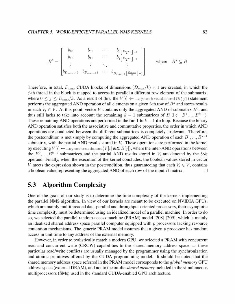
CHAPTER 5. WORK-EFFICIENT PARALLEL NMS KERNELS 82
Bk =
b00 b01 · · · b0bDmax
k c−1b10 b11 · · · b1bDmax
k c−1...
... . . . ...bDmax−10 bDmax−11 · · · bDmax−1bDmax
k c−1
where Bk ⊆ B
Therefore, in total, Dmax CUDA blocks of dimensions (Dmax/k) × 1 are created, in which thej-th thread in the block is mapped to access in parallel a different row element of the submatrix,where 0 ≤ j ≤ Dmax/k. As a result of this, the V [i] ← syncthreads and(B[j])statementperforms the aggregated AND operation of all elements on a given i-th row ofBk and stores resultsin each Vi ∈ V . At this point, vector V contains only the aggregated AND of submatrix B0, andthus still lacks to take into account the remaining k − 1 submatrices of B (i.e. B1, ..., Bk−1).These remaining AND operations are performed in the for 1 to k − 1 do loop. Because the binaryAND operation satisfies both the associative and commutative properties, the order in which ANDoperations are conducted between the different submatrices is completely irrelevant. Therefore,the postcondition is met simply by computing the aggregated AND operation of each B1, ..., Bk−1
submatrix, with the partial AND results stored in Vi. These operations are performed in the kernelby executing V [i]← syncthreads and(V [i] &&B[j]), where the inter-AND operations betweenthe B0, ..., Bk−1 submatrices and the partial AND results stored in Vi are denoted by the &&operand. Finally, when the execution of the kernel concludes, the boolean values stored in vectorV meets the expression shown in the postcondition, thus guaranteeing that each Vi ∈ V , containsa boolean value representing the aggregated AND of each row of the input B matrix.
5.3 Algorithm ComplexityOne of the goals of our study is to determine the time complexity of the kernels implementingthe parallel NMS algorithm. In view of our kernels are meant to be executed on NVIDIA GPUs,which are mainly multithreaded data-parallel and throughput-oriented processors, their asymptotictime complexity must be determined using an idealized model of a parallel machine. In order to doso, we selected the parallel random-access machine (PRAM) model [208] [209], which is mainlyan idealized shared address space parallel computer equipped with p processors lacking resourcecontention mechanisms. The generic PRAM model assumes that a given p processor has randomaccess in unit time to any address of the external memory.
However, in order to realistically match a modern GPU, we selected a PRAM with concurrentread and concurrent write (CRCW) capabilities to the shared memory address space, as theseparticular read/write conflicts are usually managed by the programmer using the synchronizationand atomic primitives offered by the CUDA programming model. It should be noted that theshared memory address space referred in the PRAM model corresponds to the global memory GPUaddress space (external DRAM), and not to the on-die shared memory included in the simultaneousmultiprocessors (SMs) used in the standard CUDA-enabled GPU architecture.
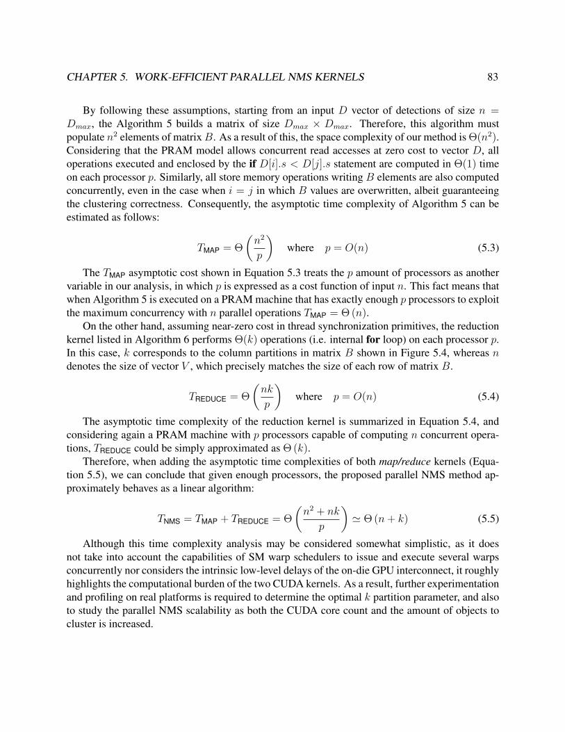
CHAPTER 5. WORK-EFFICIENT PARALLEL NMS KERNELS 83
By following these assumptions, starting from an input D vector of detections of size n =Dmax, the Algorithm 5 builds a matrix of size Dmax × Dmax. Therefore, this algorithm mustpopulate n2 elements of matrixB. As a result of this, the space complexity of our method is Θ(n2).Considering that the PRAM model allows concurrent read accesses at zero cost to vector D, alloperations executed and enclosed by the if D[i].s < D[j].s statement are computed in Θ(1) timeon each processor p. Similarly, all store memory operations writing B elements are also computedconcurrently, even in the case when i = j in which B values are overwritten, albeit guaranteeingthe clustering correctness. Consequently, the asymptotic time complexity of Algorithm 5 can beestimated as follows:
TMAP = Θ
(n2
p
)where p = O(n) (5.3)
The TMAP asymptotic cost shown in Equation 5.3 treats the p amount of processors as anothervariable in our analysis, in which p is expressed as a cost function of input n. This fact means thatwhen Algorithm 5 is executed on a PRAM machine that has exactly enough p processors to exploitthe maximum concurrency with n parallel operations TMAP = Θ (n).
On the other hand, assuming near-zero cost in thread synchronization primitives, the reductionkernel listed in Algorithm 6 performs Θ(k) operations (i.e. internal for loop) on each processor p.In this case, k corresponds to the column partitions in matrix B shown in Figure 5.4, whereas ndenotes the size of vector V , which precisely matches the size of each row of matrix B.
TREDUCE = Θ
(nk
p
)where p = O(n) (5.4)
The asymptotic time complexity of the reduction kernel is summarized in Equation 5.4, andconsidering again a PRAM machine with p processors capable of computing n concurrent opera-tions, TREDUCE could be simply approximated as Θ (k).
Therefore, when adding the asymptotic time complexities of both map/reduce kernels (Equa-tion 5.5), we can conclude that given enough processors, the proposed parallel NMS method ap-proximately behaves as a linear algorithm:
TNMS = TMAP + TREDUCE = Θ
(n2 + nk
p
)' Θ (n+ k) (5.5)
Although this time complexity analysis may be considered somewhat simplistic, as it doesnot take into account the capabilities of SM warp schedulers to issue and execute several warpsconcurrently nor considers the intrinsic low-level delays of the on-die GPU interconnect, it roughlyhighlights the computational burden of the two CUDA kernels. As a result, further experimentationand profiling on real platforms is required to determine the optimal k partition parameter, and alsoto study the parallel NMS scalability as both the CUDA core count and the amount of objects tocluster is increased.

CHAPTER 5. WORK-EFFICIENT PARALLEL NMS KERNELS 84
.global_Z23nms_mapP6float4Phf
.type_Z23nms_mapP6float4Phf,@function
.size_Z23nms_mapP6float4Phf,(.L_465 - _Z23nms_mapP6float4Phf)
.other_Z23nms_mapP6float4Phf,<no object>_Z23nms_mapP6float4Phf:.text._Z23nms_mapP6float4Phf: MOV R1, c[0x0][0x20] ; S2R R0, SR_CTAID.Y ; S2R R5, SR_TID.Y ; S2R R2, SR_CTAID.X ; S2R R3, SR_TID.X ; XMAD R5, R0, c[0x0] [0xc], R5 ; XMAD.MRG R6, R0, c[0x0] [0xc].H1, RZ ; XMAD.PSL.CBCC R0, R0.H1, R6.H1, R5 ; XMAD R3, R2, c[0x0] [0x8], R3 ; XMAD.MRG R4, R2, c[0x0] [0x8].H1, RZ ; ISCADD R8.CC, R0.reuse, c[0x0][0x140], 0x4 ; SHR R5, R0, 0x1c ; XMAD.PSL.CBCC R2, R2.H1, R4.H1, R3 ; IADD.X R9, R5, c[0x0][0x144] ; ISCADD R4.CC, R2.reuse, c[0x0][0x140], 0x4 ; SHR R3, R2, 0x1c ; IADD.X R5, R3, c[0x0][0x144] SLOT 0; LDG.E R3, [R8+0xc] SLOT 1 LDG.E R6, [R4+0xc] ; FSETP.GEU.AND P0, PT, R6, R3, PT ;
@P0 EXIT ;
LDG.E.128 R4, [R4] ; LDG.E.128 R8, [R8] ; FADD R3, R4, R6 ; FADD R7, R5, R6 ; FADD R6, R8, R10 ; FADD R13, R9.reuse, R10 ; FMNMX R12, R8, R4, !PT ; FMNMX R14, R9, R5, !PT ; FMNMX R3, R3, R6, PT ; FMNMX R7, R7, R13, PT ; FADD R3, R3, -R12 ; FADD R7, R7, -R14 ; FADD R4, R3, 1 ; FADD R7, R7, 1 ; FADD R3, R10, 1 ; FMNMX R4, RZ, R4, !PT ; FMNMX R7, RZ, R7, !PT ; FMUL R3, R3, R3 ; FMUL R4, R4, R7 ; CAL `($_Z23nms_mapP6float4Phf$__cuda_sm3x_div_rn_noftz_f32) ; ISCADD R0, R2, R0, 0xc ; FSETP.GEU.AND P0, PT, R3, c[0x0][0x150], PT ; SHR R2, R0, 0x1f ; IADD R4.CC, R0, c[0x0][0x148] ; XMAD.PSL.CLO R0, R0.H1, 0x1, RZ ; IADD.X R3, R2, c[0x0][0x14c] ; @!P0 FCMP.EQ R0, RZ, c[0x2][0x0], R10 ; MOV R2, R4 ; STG.E.U8 [R2], R0 ;
EXIT ;
(a) Map kernel
.global_Z21nms_reducePhS_i
.type_Z21nms_reducePhS_i,@function
.size_Z21nms_reducePhS_i,(.L_467 - _Z21nms_reducePhS_i)
.other_Z21nms_reducePhS_i,<no object>_Z21nms_reducePhS_i:.text._Z21nms_reducePhS_i: MOV R1, c[0x0][0x20] ; PSETP.AND.AND P1, PT, !PT, PT, PT ; S2R R4, SR_CTAID.X S2R R2, SR_TID.X ; ISCADD R0, R4, R2, 0xc ; SSY `(.L_3) SHR R2, R0, 0x1f ; IADD R0.CC, R0, c[0x0][0x140] ; IADD.X R3, R2, c[0x0][0x144] ; MOV R2, R0 ; LDG.E.U8 R0, [R2] ; IADD R4.CC, R4, c[0x0][0x148] ; IADD.X R5, RZ, c[0x0][0x14c] ; ISETP.NE.U32.AND P0, PT, R0, RZ, PT ; BAR.RED.AND 0x0, P0 ; NOP ; NOP ; NOP ; NOP ; B2R.RESULT RZ, P0 ; SEL R6, RZ, 0x1, !P0 ; STG.E.U8 [R4], R6 ;
@!P0 SYNC (*"TARGET= .L_3 "*);
LDG.E.U8 R0, [R2+0x80] ; ISETP.NE.AND P1, PT, R0, RZ, PT ; SYNC (*"TARGET= .L_3 "*)
(b) Reduce kernel (partial block view)
Figure 5.5: SASS assembly code of the proposed parallel NMS kernels (sm 62 architecture)
5.4 Static Code AnalysisIn order to determine whether the proposed parallel algorithms implementing the kernels generateor not the desired code optimizations discussed in Section 5.2, a brief static analysis of the ker-nel’s GPU assembly instructions was conducted. This analysis relied on NVIDIA’s nvdisasm tool[210], which directly worked with the .cubin CUDA binary file (an ELF file containing CUDAexecutable code sections) to parse and pretty print the assembly instructions of the target GPUarchitecture. These assembly GPU instructions are known as SASS, and should not be confusedwith the PTX (Parallel Thread eXecution) virtual instruction set [211] used to enable binary codeportability across multiple GPU generations.
Figure 5.5 shows the SASS instructions of the map/reduce kernels when targeting the sm 62
GPU architecture. As expected, the predicated instruction !PO EXIT in the map kernel yields an

CHAPTER 5. WORK-EFFICIENT PARALLEL NMS KERNELS 85
0
10
20
30
40
50
60
70
0 50 100 150 200
Theo
retic
al A
ctiv
e W
arps
per
SM
Registers Per Thread
Map Kernel (Theoretical)Reduce Kernel (Theoretical)
Actual
Figure 5.6: Theoretical active warp occupancy per SM derived from the register usage of themap/reduce kernel SASS assembly code vs. actual active warp per SM in our NMS method.
early exit, thus ending the execution flow of a given thread (implemented as a D[i].s < D[j].scheck in Algorithm 5). On the other hand, the required max and min functions used in Algorithm5 are effectively compiled to FMNMX assembly instructions. Therefore, the generated code does notrely on any conditional branch instructions that may entail unwanted performance penalties. Sim-ilarly, the reduce kernel implemented the syncthreads and() primitive using the BAR.RED.AND
assembly instruction, as it was previously discussed in Section 5.2.As a result of the SASS compilation, the register utilization of the map/reduce kernels was 15
and 8 registers, respectively, together with predicate register files P0 and P1. Consequently, theregister bank pressure for both kernels is low, and avoids a sharp reduction in active warp occu-pancy per simultaneous multiprocessor (SM). More precisely, Figure 5.6 shows theoretical valuesof warp occupancy as hypothesized by the NVIDIA Nsight Compute profiler while the usage ofregisters in the SASS code is increased for both kernels. The obtained theoretical figures determinehow our kernels would have behaved, should the amount of registers in the generated SASS code

CHAPTER 5. WORK-EFFICIENT PARALLEL NMS KERNELS 86
were higher than the actual register consumption values (15 and 8 registers, respectively). Giventhat the actual obtained register usage of both kernels are in the optimal zone of the graphs depictedin Figure 5.6, we can conclude that the code of our proposed algorithms lies in the upper bound oftheoretical warp occupancy for the selected CUDA block dimensions (see Table 5.1).
For the target sm 62 architecture the maximum number of active warps per SM supported bythe hardware is 64. This fact means the NMS kernels reach 100% of the expected theoreticaloccupancy, as register spilling is not a limiting factor. Additionaly, the parallelization pattern im-plemented in the kernels does not rely on shared memory, effectively avoiding another bottleneckthat may further reduce the occupancy on a given SM.
Kernel Block Dimensions Grid Dimensions
Map (24, 24) (24 ∗⌈|D|n
⌉, 24 ∗
⌈|D|n
⌉)
Reduce (Dmax/k) |D|
Table 5.1: Block and grid dimensions of the map/reduce CUDA kernels.
Referring again to the CUDA block dimensions, the map kernel is scheduled for executionusing a 2D block, which is tailored to the parallelization pattern described in Section 5.2. Startingfrom theD input set of detections, theB matrix is computed by specifying a grid whose dimensionsare bounded to the nearest multiple of 16 to the number of elements of D. The selected griddimensions ensures that a 16 × 16 block will generate optimal integer partitions when computingthe boolean elements of matrix B. Nevertheless, the parallelization pattern used in the reducekernel relies on unidimensional blocks for performing per row AND computations. As a result,the grid dimension precisely matches the number of elements of D (not the upper bound Dmax,which includes padding elements). Similarly, the selected block size is specifically designed forperforming Dmax/k partitions on each row of B to correctly call the required amount of times thesyncthreads and() primitive.
By following the kernel launch configuration described earlier, the theoretical values generatedby the profiler in Figure 5.6 highlight the fact that it might have not be possible to execute at allthe reduce kernel if the amount of consumed registers were higher than 64. For this reason, thegraph shows that the theoretical active warps per SM is exactly zero starting from 64 registers perthread. Luckily, this outcome never materializes, as the SASS code generated by the reduce kernelis small enough to consume only 6 registers.

CHAPTER 5. WORK-EFFICIENT PARALLEL NMS KERNELS 87
5.5 Experimental SetupSeveral evaluations were conducted to precisely determine the latency of our proposed parallelNMS method. Since the main use case of such algorithm is to enable the clustering of a high num-ber of simultaneous detections per frame on low-power embedded devices, the platforms selectedfor running the map/reduce kernels were the NVIDIA family of Tegra SoCs, which enable thescheduling, execution, profiling and debuggability of CUDA kernels with minimal efforts.
Tables 5.2 and 5.3 included below summarize the three boards used for running the experi-ments, as well as the version of the flashed NVIDIA JetPack image, which includes the requiredLinux for Tegra (L4T) OS distribution [212]. The source code of our kernels was compiled withNVIDIA’s nvcc compiler using the -O3 flag on each Tegra platform. This architectural diver-sity helped us on quantifying the scalability of the parallel algorithms implemented in our NMSkernels. More particularly, we were interested in benchmarking the NMS kernels across severalgenerations of the Tegra SoCs featuring on-die GPUs with higher CUDA core counts, improvedmicroarchitectures, memory bandwidth, bus width, and clock frequencies.
Tegra SoC CPU Cores CUDA Cores GPU Architecture GPU Clock FrequencyT124 (4+1) Arm Cortex A15 192 Kepler (GK20A) [sm 32] 72 MHz - 852 MHzT210 (4) Arm Cortex A57 256 Maxwell (GM20B) [sm 53] 76.8 MHz - 998.4 MHzT186 (2) Denver2 + (4) Arm Cortex A57 256 Pascal (GP10B) [sm 62] 114.75 MHz - 1.3 GHz
Table 5.2: Selected embedded NVIDIA Tegra platforms.
Board Tegra SoC JetPack L4T CUDA RuntimeJetson TK1 T124 v1.2 R21.5 6.5Jetson TX1 T210 v3.2.1 R28.2 9.0Jetson TX2 T186 v3.2.1 R28.2 9.0
Table 5.3: Tested embedded boards and Linux distributions.
In order to do so, the clock rate of the GPU was manually set before each kernel execution bymeans of the Linux kernel pseudo filesystem device interface (sysfs). The path for setting theGPU frequency differed depending on the Tegra SoC model included in the embedded board (seeTable 5.4). This low-level fine tuning opened us the door for comparing the throughput-orientedGPU architecture with the latency-oriented CPU cores when running both the conventional serialCPU-based NMS and the GPU-based parallel NMS at multiple clock frequencies.
Tegra SoC Filesystem PathT124 /sys/kernel/debug/clock/gbus/T210 /sys/devices/57000000.gpu/T186 /sys/devices/17000000.gp10b/
Table 5.4: sysfs path for setting up GPU clock rates.
The dynamic voltage and frequency scaling (DVFS) mechanisms of the CPUs were also dis-abled on purpose, and their corresponding clock frequencies manually set up for conducting a fair

CHAPTER 5. WORK-EFFICIENT PARALLEL NMS KERNELS 88
embedded CPU versus GPU comparison. Unfortunately, only the clustered multicore CPU designof the Tegra K1 SoC (T124) offered us the possibility of having access to an architecture packinghigh-performance out-of-order CPU cores with a low-performing and low-power CPU core (theso-called fifth companion core). The Tegra T210 SoC included in the Jetson TX1 board featuresonly four high-performance Arm Cortex A57 CPU cores. Even though that the SoC die includesfour additional in-order Arm Cortex A53 CPU cores, they were disabled on purpose during themanufacturing process. Therefore, this SoC does not provide OS-level access to a low-power clus-ter set of cores for reducing the power consumption when running background tasks, as opposed toother chips implementing Arm’s big.LITTLE technology [213]. On the other hand, the Tegra 186SoC relies on a heterogeneous architecture that combines two high-performance Armv8-compliantVLIW cores developed by NVIDIA (Denver 2) with four out-of-order Arm Cortex A57 cores. Inview of only the T124 SoC offered the possibility of running code at a true low-power CPU, webenchmarked the serial NMS code on the two CPU profiles available on that platform (i.e. high-performance CPU cores and the low-performance CPU core).
Referring again to the GPU capabilities, even though that both T210 and T186 SoCs feature256 CUDA cores, the latter one both runs at a higher clock rate and doubles the effective GPUmemory bandwidth by increasing the memory bus from 64 bits to 128 bits. This fact will enableus later to study the impact of doubling the memory bandwidth when executing on the GPU theparallel map/reduce NMS kernels.
Finally, the most important part of the evaluation was to carefully select the input datasets todemonstrate how the proposed parallel NMS is able to cope with challenging real-world situationsthat feature lots of simultaneous objects in high-resolution images and video frames. As we areinterested in human faces, we selected a 1080p input video from the SVT High Definition MultiFormat Test Set 1 (named crowd run), which was originally filmed by the Swedish Television at50 FPS using 65 mm film professional equipment. This particular video features approximately onaverage 60 simultaneous faces, but it was especially chosen because it yields hundreds of simulta-neous detections per frame after having executed a CNN-based face classifier.
Input Dataset Resolution (pixels) Typecrowd run 1920x1080 H.264 Video @ 50 FPS [00h:00m:10s]mosaic 3840x2160 H.264 Video @ 50 FPS [00h:00m:10s]oscars 4646x1800 JPEG Picture
Table 5.5: Input datasets selected for benchmarking the parallel NMS kernels.
In order to further stress out the parallel NMS kernels, we post-processed the original 1080pcrowd run video stream to generate a 3960x2160 synthetic mosaic video incorporating fourstreams on each frame (depicted in Figure 5.7), thus effectively quadrupling the number of simul-taneous detected faces. Similarly, we also decided to study in detail the scalability of parallel NMSas the number of simultaneous faces are linearly increased. For this particular experiment, weselected a picture of the 83rd Academy Awards Nominees 2 captured during the Oscars ceremony
1Sveriges Television High Definition Multi Format Test Set repository (ftp://vqeg.its.bldrdoc.gov/HDTV/SVT_MultiFormat/)
283rd Academy Awards Nominees picture (http://tinyurl.com/o5n97ra/)
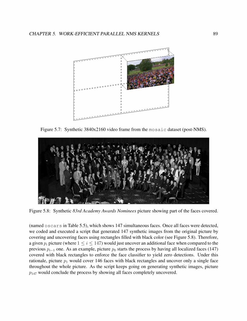
CHAPTER 5. WORK-EFFICIENT PARALLEL NMS KERNELS 89
Figure 5.7: Synthetic 3840x2160 video frame from the mosaic dataset (post-NMS).
Figure 5.8: Synthetic 83rd Academy Awards Nominees picture showing part of the faces covered.
(named oscars in Table 5.5), which shows 147 simultaneous faces. Once all faces were detected,we coded and executed a script that generated 147 synthetic images from the original picture bycovering and uncovering faces using rectangles filled with black color (see Figure 5.8). Therefore,a given pi picture (where 1 ≤ i ≤ 147) would just uncover an additional face when compared to theprevious pi−1 one. As an example, picture p0 starts the process by having all localized faces (147)covered with black rectangles to enforce the face classifier to yield zero detections. Under thisrationale, picture p1 would cover 146 faces with black rectangles and uncover only a single facethroughout the whole picture. As the script keeps going on generating synthetic images, picturep147 would conclude the process by showing all faces completely uncovered.

CHAPTER 5. WORK-EFFICIENT PARALLEL NMS KERNELS 90
5.6 ResultsAs it was previously discussed, first we started by determining how the latency of the GPU-basedparallel NMS algorithm compares against the traditional serialized version of OpenCV’s O(n2)greedy NMS, which is still used in many works [214] for clustering the bounding boxes obtainedafter inferencing CNN classifiers. This comparison was conducted by executing both NMS algo-rithms on the Jetson TK1 board using as an input the oscars dataset picture. More precisely,both NMS algorithms were executed at multiple frequencies on the two different CPU clustersavailable in the T124 SoC (i.e. high-performance CPU-G cluster, and low-power CPU-LP cluster)by properly setting up the parameters in the sysfs Linux kernel interface. The CPU-LP coreclock frequency ranges between 51 MHz and 1 GHz, while a given CPU-G core ranges between204 MHz and 2.3 GHz. Similarly, the GPU clock ranges between 72 MHz and 850 MHz, as Table5.2 shows. The results of this experiment are shown below in Figure 5.9.
0
100
200
300
400
500
600
0 500 1000 1500 2000 2500
Non
-max
imum
Sup
pres
sion
Tim
e (m
s)
Frequency (MHz)
[83rd Academy Award Nominees]
GPUCPU-GCPU-LP
Figure 5.9: NMS latency on GPU, CPU-LP and CPU-G cores for the selected oscars dataset.

CHAPTER 5. WORK-EFFICIENT PARALLEL NMS KERNELS 91
0
20
40
60
80
100
120
140
160
0 200 400 600 800 1000 1200 1400
Non
-max
imum
Sup
pres
sion
Tim
e (m
s)
Frequency (MHz)
[83rd Academy Award Nominees]
TK1TX1TX2
Figure 5.10: NMS latency when processing the oscars dataset on the GPUs included in theselected Tegra SoCs.
The graph in Figure 5.9 clearly shows that a GPU clocked at 50% of its maximum frequencyoutperforms both CPU types also when they are operating at 50% of its peak operating frequency.For this experiment, the overhead of memory allocations and initializations was not taken into ac-count, and only the pure kernel execution time was considered. It should be noted that for battery-powered fanless solutions the chip must be underclocked or automatically managed by the under-lying DVFS subsystem to avoid excessive overheating. Unsurprisingly, the GPU shows an ad-vantage, especially for GPU-based object detection and recognition pipelines, in which unwantedCPU/GPU memory transfers slowdown the throughput of real-time applications, as it would unde-sirably happen when relying on the serialized NMS targeting CPUs.
On the other hand, the proposed parallel NMS was evaluated on all GPUs of the selectedTegra platforms, also by varying the clock rate of the GPU before executing the kernels during theexperiments, and using the same input dataset (oscars). The results of these experiments aresummarized in Figure 5.10. The reported latencies, aggregate the combined execution time of the
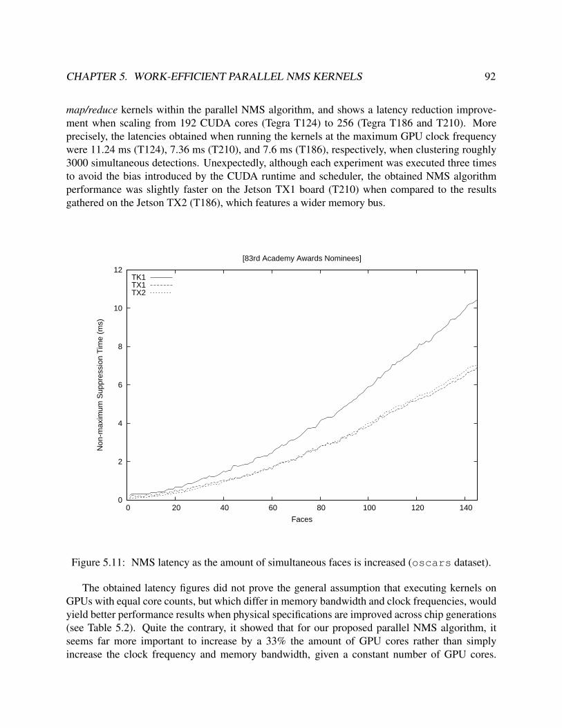
CHAPTER 5. WORK-EFFICIENT PARALLEL NMS KERNELS 92
map/reduce kernels within the parallel NMS algorithm, and shows a latency reduction improve-ment when scaling from 192 CUDA cores (Tegra T124) to 256 (Tegra T186 and T210). Moreprecisely, the latencies obtained when running the kernels at the maximum GPU clock frequencywere 11.24 ms (T124), 7.36 ms (T210), and 7.6 ms (T186), respectively, when clustering roughly3000 simultaneous detections. Unexpectedly, although each experiment was executed three timesto avoid the bias introduced by the CUDA runtime and scheduler, the obtained NMS algorithmperformance was slightly faster on the Jetson TX1 board (T210) when compared to the resultsgathered on the Jetson TX2 (T186), which features a wider memory bus.
0
2
4
6
8
10
12
0 20 40 60 80 100 120 140
Non
-max
imum
Sup
pres
sion
Tim
e (m
s)
Faces
[83rd Academy Awards Nominees]
TK1TX1TX2
Figure 5.11: NMS latency as the amount of simultaneous faces is increased (oscars dataset).
The obtained latency figures did not prove the general assumption that executing kernels onGPUs with equal core counts, but which differ in memory bandwidth and clock frequencies, wouldyield better performance results when physical specifications are improved across chip generations(see Table 5.2). Quite the contrary, it showed that for our proposed parallel NMS algorithm, itseems far more important to increase by a 33% the amount of GPU cores rather than simplyincrease the clock frequency and memory bandwidth, given a constant number of GPU cores.

CHAPTER 5. WORK-EFFICIENT PARALLEL NMS KERNELS 93
0
2
4
6
8
10
12
0 500 1000 1500 2000 2500
Non
-max
imum
Sup
pres
sion
Tim
e (m
s)
Detections
[83rd Academy Awards Nominees]
TK1TX1TX2GTX 1060Tesla T4
Figure 5.12: NMS latency on growing number of detections (oscars dataset).
As an example, the T186 GPU must be clocked at 1.3 GHz to achieve the performance figuresyielded by the T210 chip when clocked at 998.4 MHz. Therefore, the GPU scalability of parallelNMS is more sensitive to the number of cores (a 33% increase in GPU cores yields a 55% latencyreduction), rather than to the improvements of the memory subsystem, thus highlighting that kernelcode bottlenecks are skewed towards the availability and quantity of ALUs included in the GPUs(i.e. compute-bound kernel).
However, since the main benefit of the parallel NMS is the potential and flexibility offered forhandling the clustering of detections in workloads featuring huge amounts of simultaneous objects,we decided to determine the scalability of the map/reduce kernels as the quantity of simultaneousfaces are increased. These experiments involved executing the parallel NMS kernels on the selectedTegra platforms using as an input the synthetic set of pictures featuring covered faces (as it is shownin Figure 5.8). The results of such experiments are summarized in the graph depicted in Figure5.11, and are consistent with the previous observation that emphasizes the importance of the GPUCUDA core count (both TX1 and TX2 outperform the older TK1). Hence, the slopes of both TX1

CHAPTER 5. WORK-EFFICIENT PARALLEL NMS KERNELS 94
and TX2 graphs are greatly reduced when compared to the baseline TK1 graph, thus proving thatour proposed parallel NMS algorithm properly scales as the CUDA core count is increased. Inorder to further illustrate this fact, Figure 5.12 also shows an extra reduction of the graph slopewhen the parallel NMS algorithm is executed on a discrete NVIDIA GeForce GTX 1060 GPUfeaturing 1280 CUDA cores over a growing number of detections, and a further reduction whenexecuted on a Tesla T4 GPU with 2560 CUDA cores. More particularly, the GTX 1060 yieldedan 8.11X speed up over the TK1, 5.38X (TX2) and 5.23X (TX1), respectively. And the Tesla T4yielded a 24.59X speed up over the TK1, 15.91X over TX2, and 16.44X over TX1.
NMS Latency (ms)Discrete GPU CUDA Cores Clock Rate n = 200 n = 1027 n = 2895
GeForce GTX 1060 1280 1.70 GHz 0.107 0.324 1.313Tesla T4 2560 1.59 GHz 0.024 0.088 0.430
Table 5.6: NMS latency on discrete GPUs when clustering n detections (oscars dataset).
As Table 5.6 shows, discrete GPUs clocked at roughly the same frequencies, and relying oncomparable memory subsystem technologies (i.e. GDDR5 -GTX 1060- vs. GDDR6 -Tesla T4-),but with increased number of CUDA cores trigger substantial reductions in the NMS latency. As aresult, increasing by a factor of 2 the amount of cores in the underlying hardware resources reducesthe NMS execution latency by a factor of 3 for 2895 detections, effectively proving the scalabilityof our parallel NMS method as the amount of cores keeps increasing.
These results are in line with our initial expectations about the time complexity of the parallelNMS. On these latter experiments, the GPU kernels were also compiled and benchmarked bysetting k = 32 and Dmax = 4096 (upper limit used for the GPU memory allocations required bymatrix B and vector V ).
In order to further study and optimize the NMS reduction kernel (Algorithm 6), several exper-iments were carried out to study the impact of parameter k with the aim of finding which partitionsize minimizes the latency in the NMS reduction kernel. Table 5.7 summarizes the obtained resultson each SoC of the selected Tegra platforms on the oscars dataset.
Reduction Kernel Latency (ms)k TK1 TX1 TX24 2.972 1.641 1.6928 2.311 1.394 1.46516 2.027 1.301 1.36932 1.842 1.273 1.32664 3.234 1.654 1.520
128 5.602 2.775 2.035256 10.695 4.440 3.895
Table 5.7: NMS reduction kernel latency depending on the k parameter.
According to the experiments, the optimal partition size yielding minimal latencies would bek = 32, which was precisely the value used for obtaining the previously shown graphs (Fig-ure 5.11 and 5.12). Interestingly, these results challenge conventional wisdom, as it is increas-ingly less costly to call k times syncthreads and()in the for loop when 4 ≤ k ≤ 32. As

CHAPTER 5. WORK-EFFICIENT PARALLEL NMS KERNELS 95
Dmax
k = 32
k = 4
Figure 5.13: Thread synchronizations computed on a given B matrix row (k=32 and k=4).
thread synchronization is typically slow (i.e. theoretically, a barrier should be avoided if possi-ble), it is considered counter-intuitive that an increasing number of thread synchronization oper-ations could contribute to reduce the execution time. Taking into account that NVIDIA GPUsoffer architectural support at the ISA level for implementing these primitives, and GPU hard-ware thread synchronization primitives work at the CUDA block level, the amount of Dmax/kpartitions created per matrix row effectively serves as a mechanism for fine-tuning the quantityof inter-block syncthreads and()calls executed in parallel (represented as arc symbols inFigure 5.13). A comparison of the granularity of such thread synchronizations is highlighted inthe aforementioned figure, which illustrates how the k parameter greatly affects the number ofsyncthreads and()calls executed in parallel, as the amount of CUDA blocks created varies.
Nevertheless, when k > 32, as both Table 5.7 and Figure 5.14 depict, the NMS reduction ker-nel latency keeps growing due to unoptimal CUDA block partitions when processing the B inputmatrix.
Average NMS Latency (ms)Tegra SoC k Map Reduce Total
TK1
4 5.17 2.41 7.788 5.16 1.87 7.22
16 5.17 1.64 6.9732 5.17 1.54 6.88
TX1
4 3.74 1.34 4.848 3.37 1.11 4.57
16 3.38 1.03 4.5332 3.38 1.00 4.48
TX2
4 3.52 1.37 4.938 3.50 1.16 4.71
16 3.50 1.07 4.6132 3.49 1.03 4.56
Table 5.8: Average NMS latencies on TK1, TX1 and TX2 SoCs (mosaic dataset).
Finally, the crowd run and mosaic datasets described in Table 5.5 were also used as aninput of the map/reduce NMS kernels. The main objective of experimenting with those datasetswas to characterize the underlying performance scalability of both kernels when localizing facesin videos featuring challenging real-world scenarios. Additionally, further experimentation was

CHAPTER 5. WORK-EFFICIENT PARALLEL NMS KERNELS 96
2
4
6
8
10
12
4 8 16 32 64 128 256
Red
uctio
n K
erne
l Lat
ency
(m
s)
k
TK1TX1TX2
Figure 5.14: NMS reduction kernel latency according to parameter k.
carried out to determine the execution time distribution of both Algorithm 5 (map kernel) andAlgorithm 6 (reduce kernel).
As it was done with the oscars dataset picture, the NMS kernels were benchmarked overtime on the selected Tegra platforms after having firstly decoded H.264 video frames, and laterperformed face detection. The obtained results are summarized in Figure 5.15, which shows boththe number of faces detected per frame (top dashed line), and the aggregated latency of the parallelNMS kernels when executed on the selected SoCs (three lines shown at the bottom). Therefore,the H.264 decoding latency was not taken into account, thus profiling only the map/reduce kernelsat the low level.
On this particular dataset (crowd run), the amount of detected faces per frame ranged be-tween 360 and 698 detections. Again, these experiments were carried out by setting k = 32 andDmax = 4096 when clustering detected faces. The aggregated latencies yielded by the parallelNMS were less than 2 ms. More particularly, it ranged between 0.5 ms and 1.8 ms when exe-cuted on the Jetson TK1 (T124). When switching to Jetson TX1 (T210) and Jetson TX2 (T186)platforms, latencies were reduced a further 50% due to the increased GPU core counts. As it also

CHAPTER 5. WORK-EFFICIENT PARALLEL NMS KERNELS 97
0
1
2
3
4
5
6
7
8
0 50 100 150 200 250 300 350 400 0
100
200
300
400
500
600
700
800
Non
-max
imum
Sup
pres
sion
Tim
e (m
s)
Num
ber o
f Det
ectio
ns
Video Frame
[crowd_run] 1920x1080 @ 50 FPS
TK1TX1TX2 #det
TK1TX1
TX2
Figure 5.15: NMS latency per frame vs. #det number of detections (crowd run).
happened with previous experiments, there were no major performance improvements betweenTX1 and TX2 platforms when executing the parallel NMS algorithm. The latency reduction onTX2 was on average 6.25% lower than on TX1 and very close to 0.5 ms, while the precise stan-dard deviation of measured latencies was 0.18 ms on both platforms.
Therefore, in order to further spot differences and analyze the potential benefits of the improvedT186 SoC, it might be necessary to saturate the GPU resources. Moreover, the mosaic videodataset was used as an input to quadruple the number of simultaneous detections per frame, sothat the amount of thread reductions per row triggered by the NMS reduction kernel is greaterthan one. The results of these experiments are summarized in Table 5.8, which details the averagelatencies for both map and reduce kernels after having executed them on a frame per frame basis.Additionally, Table 5.8 reports how the execution time of the parallel NMS kernels was affectedby parameter k on the selected Tegra platforms.
According to the obtained measurements, after quadrupling the amount of simultaneous faces,the main bottleneck of the parallel NMS algorithm lies on the construction of matrix B, which isperformed in Algorithm 5 (map kernel). This performance penalty is noticeable in Figure 5.16,
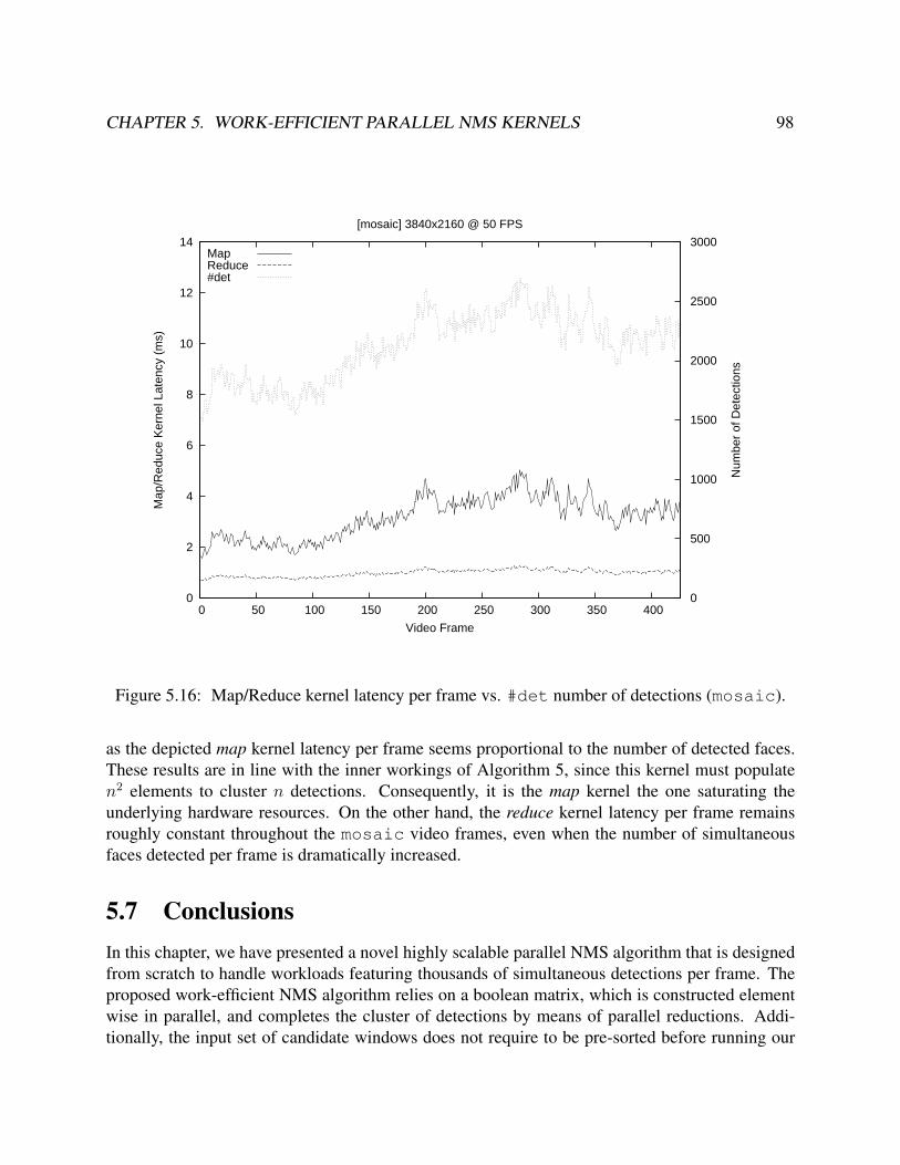
CHAPTER 5. WORK-EFFICIENT PARALLEL NMS KERNELS 98
0
2
4
6
8
10
12
14
0 50 100 150 200 250 300 350 400 0
500
1000
1500
2000
2500
3000
Map
/Red
uce
Ker
nel L
aten
cy (
ms)
Num
ber
of D
etec
tions
Video Frame
[mosaic] 3840x2160 @ 50 FPS
MapReduce#det
Figure 5.16: Map/Reduce kernel latency per frame vs. #det number of detections (mosaic).
as the depicted map kernel latency per frame seems proportional to the number of detected faces.These results are in line with the inner workings of Algorithm 5, since this kernel must populaten2 elements to cluster n detections. Consequently, it is the map kernel the one saturating theunderlying hardware resources. On the other hand, the reduce kernel latency per frame remainsroughly constant throughout the mosaic video frames, even when the number of simultaneousfaces detected per frame is dramatically increased.
5.7 ConclusionsIn this chapter, we have presented a novel highly scalable parallel NMS algorithm that is designedfrom scratch to handle workloads featuring thousands of simultaneous detections per frame. Theproposed work-efficient NMS algorithm relies on a boolean matrix, which is constructed elementwise in parallel, and completes the cluster of detections by means of parallel reductions. Addi-tionally, the input set of candidate windows does not require to be pre-sorted before running our

CHAPTER 5. WORK-EFFICIENT PARALLEL NMS KERNELS 99
method, as the proposed map kernel always selects the representative with the highest score amongall detections within the cluster while building the boolean matrix.
The obtained performance results show that the proposed map/reduce kernels are computebound, and properly scale on embedded GPUs as the amount of CUDA cores is increased. Asa result of this, the parallel NMS algorithm is capable of clustering 1024 simultaneous detectedfaces per frame in roughly 1 ms on both Tegra X1 (T210) and Tegra X2 (T186) on-die GPUs,while taking 2 ms on Tegra K1 (T124). Therefore, the parallel NMS execution time is effectivelyreduced 53% when the GPU computing resources are increased by a 33% from 192 to 256 CUDAcores. Thanks to additional experimentation, we also proved that this ratio is further improved asthe amount simultaneous detections per frame keeps growing (e.g. 2048 detections and beyond).
Moreover, when the proposed parallel NMS method is executed on powerful discrete GPUswith high core counts and complex memory hierarchies, the execution time is even more drasticallyreduced. Interestingly, our obtained results show that doubling the amount of cores from 1280 to2560 reduces the NMS execution time by at least a factor of three, which is even more pronouncedthan in the embedded GPU platforms. In this latter scenario, the parallel NMS is capable ofclustering roughly 3000 candidate windows in less than 0.5 ms. These results show that our NMSmethod yields a minimal footprint in a GPU-only object recognition pipeline, as its executionconsumes only 1% of the 40 ms hard deadline required for the real-time processing of video feedsat 25 FPS.
As future work, we plan to study the performance impact of implementing thread group syn-chronization in the reduction kernel grid. However, as this feature is only available on Pascal andVolta GPU architectures, it would sacrifice portability of the parallel NMS kernel across legacyGPU computing platforms.

100
Chapter 6
Conclusions
In this thesis, we have explored several low-level parallelization techniques to enable the execu-tion of face detection on heterogeneous GPU platforms at a high throughput. Since the thesiswas started, and our first contributions were made, the field has experienced an explosion in theutilization of GPGPU computing for executing workloads in the areas of computer vision, ma-chine learning, and most notably, convolutional neural networks. This fact proved that we clearlysucceeded on anticipating this major computing trend before it happened. Nowadays, almost allstate-of-the-art machine learning libraries involved in such workloads [67], [72], [136] rely onCUDA and OpenCL kernels for parallelizing computations. It is also now very common to offloadcomputations to remote clusters and clouds of discrete GPUs [215] for conducting video analytics,biometric template matching, object attribute search, and training models.
Although boosting-based frameworks were surpassed by highly accurate deep neural networks,they are still useful in niche applications such as object or facial tracking for surveillance, and dueto its early discard properties, they still may play a key role for solving the problem of facialdetection at UHD resolutions. For this reason, we think the parallelization methods presented inChapter 3 and 4 are relevant, and further study should be devoted to improve split strategies duringthe evaluation of feature cascades. More sophisticated approaches could involve prefetching andstage prediction during the evaluation, which would enable additional on-die caching.
All GPU kernels presented in this thesis have proven to be scalable across several generationsof GPU platforms. The experiments carried out in our original research publications were up-dated for this dissertation on newer platforms, and their performance was significantly boosted ina completely transparent manner, as the amount of cores and memory bandwidth were linearlyimproved. Moreover, the low latencies obtained when running our kernels in combination with theintroduced coarse and fine-grained parallelization allows us to perform facial analytics on multiplevideo streams in real time on a single device.
It could be argued that the only platforms and programming models we have studied are theones targeting NVIDIA GPU devices. However, from a low-level hardware perspective, they areheterogeneous, as they include multiple programmable computational units, on-die memories andblocks (e.g. video decoding engines, tensor cores, and texture units). In theory, all previouslypresented parallelization strategies are valid for any massively parallel multithreaded architecture

CHAPTER 6. CONCLUSIONS 101
capable of executing OpenCL kernels. Newer platforms such as Intel’s Xe or AMD’s RDNAmay be good candidates for efficiently running the contributed kernels with minimal adaptations.Although emerging discrete neural network accelerator hardware may beat GPU performance andpower efficiency when running both training and inference, they are not capable of executingtraditional computer vision algorithms nor running any other kind of general-purpose kernels. Forthis reason, we believe that high-end discrete GPUs will still be extensively used in the futureif transistor density and memory bandwidth keeps improving. Additional enhancements couldinvolve chiplet design structured in multi-chip modules (MCM) to push the boundaries of themassively parallel many-thread architecture.
On the other hand, we also presented in Chapter 5 a novel and highly scalable parallel NMSmethod that is useful not just for facial recognition pipelines targeting surveillance applications,but also for autonomous driving, as it is designed for handling workloads featuring hundreds ofsimultaneous detections. The contributed algorithm, as we have proved, is fast and lightweightenough for running on an embedded SoC targeting real-time applications. Moreover, we also reliedon synchronized AND barrier instructions to perform reductions and cluster detections. To the bestof our knowledge, this is the first time that such synchronization method has been succesfully usedto apply parallel reductions.
Other upcoming architectures that have not been properly studied yet by academia but may alsooffer potential for efficiently running parallel face detection algorithms are processing-in-memory(PIM) devices [216]. These new technologies involve DRAM and Flash memories and embedALUs close to the memory cells to speed up computations by minimizing data movement bottle-necks. Currently, the most recent works on such platforms are mostly focused on bioinformat-ics [217], graph processing [218] or string matching to optimize database queries [219]. However,these studies are still conducted on cycle-accurate performance simulators, and early manufac-tured attempts such as Micron’s Automata Processor [220] have been discontinued. We think thatmemory-bound features such as NPD involving little computations offer a great potential whenported to PIM devices when used in combination with ensemble learning. Also, stacked CMOSsensors [221], in which DRAM and computational logic are vertically combined through-siliconvias (TSV) in multiple layers could leverage NPD features in a power-efficient manner to performfacial detection in camera equipment.
As a final conclusion, we expect that automated facial recognition systems partially based onsome of the techniques presented in this thesis will be deployed in public areas such as train stationsor airports to conduct ethical surveillance activities and live matching against blacklists. Althoughface detection could be implemented by means of a low-power neural network accelerator inte-grated within smart surveillance IP cameras (i.e. edge computing [222]), there are hundreds ofmillions of conventional CCTV cameras already deployed worldwide [223]. Therefore, in orderto avoid replacement costs, software products that retrieve video feeds from remote IP cameras byperforming facial analytics processing on high-end GPUs are still at the first stage of developmentand offer a great market potential.

102
Bibliography
[1] J. L. Hennessy and D. A. Patterson, “A New Golden Age for Computer Architecture,”Communications of the ACM, vol. 62, no. 2, pp. 48–60, 2019.
[2] W. Chen, S. Ray, J. Bhadra, M. Abadir, and L.-C. Wang, “Challenges and Trends in Mod-ern SoC Design Verification,” IEEE Design & Test, vol. 34, no. 5, pp. 7–22, 2017.
[3] W. A. Wulf and S. A. McKee, “Hitting the Memory Wall: Implications of the Obvious,”ACM SIGARCH Computer Architecture News, vol. 23, no. 1, pp. 20–24, 1995.
[4] J. E. Stone, D. Gohara, and G. Shi, “OpenCL: A Parallel Programming Standard for Het-erogeneous Computing Systems,” Computing in Science & Engineering, vol. 12, no. 3,p. 66, 2010.
[5] NVIDIA Corp., NVIDIA CUDA C Programming Guide, https://docs.nvidia.com/pdf/CUDA_C_Programming_Guide.pdf, 2018.
[6] Xilinx Inc., Xilinx Versal Prime Series, https://www.xilinx.com/products/silicon-devices/acap/, 2019.
[7] NVIDIA Corp., NVIDIA Jetson Xavier, https://developer.nvidia.com/jetson-xavier,2018.
[8] P. Viola and M. Jones, “Rapid object detection using a boosted cascade of simple features,”in IEEE Conference on Computer Vision and Pattern Recognition, IEEE, 2001.
[9] Schapire, Robert E, “The Boosting Approach to Machine Learning: An Overview,” in Non-linear Estimation and Classification, Springer, 2003, pp. 149–171.
[10] F. C. Crow, “Summed-area Tables for Texture Mapping,” in ACM SIGGRAPH ComputerGraphics, ACM, vol. 18, 1984, pp. 207–212.
[11] H. Bay, A. Ess, T. Tuytelaars, and L. Van Gool, “Speeded-up Robust Features,” ComputerVision and Image Understanding, vol. 110, no. 3, pp. 346–359, 2008.
[12] P. Dollar, Z. Tu, P. Perona, and S. Belongie, “Integral Channel Features,” 2009.
[13] C. Zhang and Z. Zhang, “Boosting-Based Face Detection and Adaptation,” Synthesis Lec-tures on Computer Vision, vol. 2, no. 1, pp. 1–140, 2010.
[14] S. Zafeiriou, C. Zhang, and Z. Zhang, “A Survey on Face Detection in the Wild: Past,Present and Future,” Computer Vision and Image Understanding, vol. 138, pp. 1–24, 2015.

BIBLIOGRAPHY 103
[15] L. Breiman, “Random Forests,” Machine Learning, vol. 45, no. 1, pp. 5–32, 2001.
[16] J. H. Friedman, “Stochastic Gradient Boosting,” Computational Statistics & Data Analysis,vol. 38, no. 4, pp. 367–378, 2002.
[17] C. Cortes and V. Vapnik, “Support Vector Machine,” Machine Learning, vol. 20, no. 3,pp. 273–297, 1995.
[18] S. Liao, A. K. Jain, and S. Z. Li, “A Fast and Accurate Unconstrained Face Detector,” IEEETransactions on Pattern Analysis and Machine Intelligence, vol. 38, no. 2, pp. 211–223,2015.
[19] R. Lienhart and J. Maydt, “An Extended Set of Haar-like Features For Rapid Object Detec-tion,” in Proceedings of the International Conference on Image Processing, IEEE, vol. 1,2002, pp. 900–903.
[20] S. Li, L. Zhu, Z. Zhang, A. Blake, H. Zhang, and H. Shum, “Statistical Learning of Multi-view Face Detection,” European Conference on Computer Vision, pp. 117–121, 2006.
[21] M. Jones and P. Viola, “Fast Multi-view Face Detection,” Mitsubishi Electric Research LabTR-20003-96, vol. 3, 2003.
[22] T. Mita, T. Kaneko, and O. Hori, “Joint Haar-like Features for Face Detection,” in IEEEInternational Conference on Computer Vision, IEEE, vol. 2, 2005, pp. 1619–1626.
[23] D. Zhang, S. Z. Li, and D. Gatica-Perez, “Real-time Face Detection Using Boosting in Hi-erarchical Feature Spaces,” in Proceedings of the 17th International Conference on PatternRecognition, IEEE, vol. 2, 2004, pp. 411–414.
[24] T. Ojala, M. Pietikainen, and D. Harwood, “A Comparative Study of Texture Measureswith Classification Based on Featured Distributions,” Pattern Recognition, vol. 29, no. 1,pp. 51–59, 1996.
[25] T. Ojala, M. Pietikainen, and T. Maenpaa, “Multiresolution Gray-scale and Rotation In-variant Texture Classification with Local Binary Patterns,” IEEE Transactions on patternanalysis and machine intelligence, vol. 24, no. 7, pp. 971–987, 2002.
[26] T. Ahonen, A. Hadid, and M. Pietikainen, “Face Recognition with Local Binary Patterns,”Proceedings of the 8th European Conference on Computer Vision, pp. 469–481, 2004.
[27] L. Zhang, R. Chu, S. Xiang, S. Liao, and S. Li, “Face detection based on multi-block LBPrepresentation,” Advances in Biometrics, pp. 11–18, 2007.
[28] J. Li, T. Wang, and Y. Zhang, “Face Detection using SURF Cascade,” in IEEE InternationalConference on Computer Vision Workshops, IEEE, 2011, pp. 2183–2190.
[29] L. Bourdev and J. Brandt, “Robust Object Detection Via Soft Cascade,” in IEEE Confer-ence on Computer Vision and Pattern Recognition, IEEE, vol. 2, 2005, pp. 236–243.
[30] N. Dalal and B. Triggs, “Histograms of Oriented Gradients for Human Detection,” in IEEEComputer Vision and Pattern Recognition, IEEE, vol. 1, 2005, pp. 886–893.

BIBLIOGRAPHY 104
[31] B. Jun, I. Choi, and D. Kim, “Local Transform Features and Hybridization for AccurateFace and Human Detection,” IEEE Transactions on Pattern Analysis and Machine Intelli-gence, vol. 35, no. 6, pp. 1423–1436, 2012.
[32] O. Deniz, G. Bueno, J. Salido, and F. De la Torre, “Face Recognition using Histograms ofOriented Gradients,” Pattern Recognition Letters, vol. 32, no. 12, pp. 1598–1603, 2011.
[33] M. Mathias, R. Benenson, M. Pedersoli, and L. Van Gool, “Face Detection without Bellsand Whistles,” in European Conference on Computer Vision, Springer, 2014, pp. 720–735.
[34] G. Ekman, “Weber’s Law and Related Functions,” The Journal of Psychology, vol. 47,no. 2, pp. 343–352, 1959.
[35] V. Jain and E. Learned-Miller, “FDDB: A Benchmark for Face Detection in UnconstrainedSettings,” University of Massachusetts, Amherst, Tech. Rep. UM-CS-2010-009, 2010.
[36] R. Meir and G. Ratsch, “An Introduction to Boosting and Leveraging,” Advanced Lectureson Machine Learning, pp. 118–183, 2003.
[37] J. Friedman, T. Hastie, and R. Tibshirani, “Additive Logistic Regression: A Statistical Viewof Boosting,” The Annals of Statistics, vol. 28, no. 2, pp. 337–407, 2000.
[38] Y. Freund and R. Schapire, “A Desicion-theoretic Generalization of On-line Learning andan Application to Boosting,” in Computational Learning Theory, Springer, 1995, pp. 23–37.
[39] R. Lienhart, A. Kuranov, and V. Pisarevsky, “Empirical Analysis of Detection Cascades ofBoosted Classifiers for Rapid Object Detection,” Pattern Recognition, pp. 297–304, 2003.
[40] Y. Pang, Y. Yuan, X. Li, and J. Pan, “Efficient HOG Human Detection,” Signal Processing,vol. 91, no. 4, pp. 773–781, 2011.
[41] M. Ratsch, S. Romdhani, and T. Vetter, “Efficient Face Detection by a Cascaded SupportVector Machine using Haar-like Features,” in Pattern Recognition, Springer, 2004, pp. 62–70.
[42] B. Heisele, T. Serre, S. Prentice, and T. Poggio, “Hierarchical Classification and FeatureReduction for Fast Face Detection with Support Vector Machines,” Pattern Recognition,vol. 36, no. 9, pp. 2007–2017, 2003.
[43] J. Yan, “Ensemble SVM Regression-based Multi-view Face Detection System,” in IEEEWorkshop on Machine Learning for Signal Processing, IEEE, 2007, pp. 163–169.
[44] A. Krizhevsky, I. Sutskever, and G. E. Hinton, “ImageNet Classification with Deep Con-volutional Neural Networks,” in Advances in neural information processing systems, 2012,pp. 1097–1105.
[45] J. Gu, Z. Wang, J. Kuen, L. Ma, A. Shahroudy, B. Shuai, T. Liu, X. Wang, G. Wang, J. Cai,et al., “Recent Advances in Convolutional Neural Networks,” Pattern Recognition, vol. 77,pp. 354–377, 2018.
[46] I. Goodfellow, Y. Bengio, and A. Courville, Deep Learning. MIT Press, 2016.

BIBLIOGRAPHY 105
[47] F. Schroff, D. Kalenichenko, and J. Philbin, “FaceNet: A Unified Embedding for FaceRecognition and Clustering,” in Proceedings of the IEEE Conference on Computer Visionand Pattern Recognition, 2015, pp. 815–823.
[48] N. Srivastava, G. Hinton, A. Krizhevsky, I. Sutskever, and R. Salakhutdinov, “Dropout:A Simple Way to Prevent Neural Networks from Overfitting,” The Journal of MachineLearning Research, vol. 15, no. 1, pp. 1929–1958, 2014.
[49] X. Glorot and Y. Bengio, “Understanding the Difficulty of Training Deep FeedforwardNeural Networks,” in Proceedings of the 13th International Conference on Artificial Intel-ligence and Statistics, 2010, pp. 249–256.
[50] C. Szegedy, W. Liu, Y. Jia, P. Sermanet, S. Reed, D. Anguelov, D. Erhan, V. Vanhoucke,and A. Rabinovich, “Going Deeper with Convolutions,” in Proceedings of the IEEE Con-ference on Computer Vision and Pattern Recognition, 2015, pp. 1–9.
[51] K. Simonyan and A. Zisserman, “Very Deep Convolutional Networks for Large-scale Im-age Recognition,” arXiv preprint arXiv:1409.1556, 2014.
[52] K. He, X. Zhang, S. Ren, and J. Sun, “Deep Residual Learning for Image Recognition,” inProceedings of the IEEE Conference on Computer Vision and Pattern Recognition, 2016,pp. 770–778.
[53] A. G. Howard, M. Zhu, B. Chen, D. Kalenichenko, W. Wang, T. Weyand, M. Andreetto,and H. Adam, “Mobilenets: Efficient Convolutional Neural Networks for Mobile VisionApplications,” arXiv preprint arXiv:1704.04861, 2017.
[54] R. Girshick, J. Donahue, T. Darrell, and J. Malik, “Rich Feature Hierarchies for AccurateObject Detection and Semantic Segmentation,” in Proceedings of the IEEE Conference onComputer Vision and Pattern Recognition, 2014, pp. 580–587.
[55] S. Ren, K. He, R. Girshick, and J. Sun, “Faster R-CNN: Towards Real-time Object Detec-tion with Region Proposal Networks,” IEEE Transactions on Pattern Analysis and MachineIntelligence, vol. 39, no. 6, pp. 1137–1149, 2017.
[56] J. Dai, Y. Li, K. He, and J. Sun, “R-FCN: Object Detection via Region-based Fully Convo-lutional Networks,” in Advances in Neural Information Processing Systems, 2016, pp. 379–387.
[57] W. Liu, D. Anguelov, D. Erhan, C. Szegedy, S. Reed, C.-Y. Fu, and A. C. Berg, “SSD:Single Shot Multibox Detector,” in European Conference on Computer Vision, Springer,2016, pp. 21–37.
[58] J. Redmon and A. Farhadi, “YOLOv3: An Incremental Improvement,” arXiv preprintarXiv: 1804.02767, 2018.
[59] S. Zhang, X. Wang, Z. Lei, and S. Z. Li, “Faceboxes: A CPU Real-time and AccurateUnconstrained Face Detector,” Neurocomputing, vol. 364, pp. 297–309, 2019.
[60] Y. Jia, “Learning Semantic Image Representations at a Large Scale,” PhD thesis, UCBerkeley, 2014.
BIBLIOGRAPHY 106
[61] NVIDIA Corp., NVIDIA cuFFT, https://developer.nvidia.com/cufft, 2018.
[62] Y. Li, J. Dongarra, and S. Tomov, “A Note on Auto-tuning GEMM for GPUs,” in Interna-tional Conference on Computational Science, Springer, 2009, pp. 884–892.
[63] A. Lavin and S. Gray, “Fast Algorithms for Convolutional Neural Networks,” in Proceed-ings of the IEEE Conference on Computer Vision and Pattern Recognition, 2016, pp. 4013–4021.
[64] S. Han, H. Mao, and W. J. Dally, “Deep Compression: Compressing Deep Neural Net-works with Pruning, Trained Quantization and Huffman coding,” arXiv:1510.00149, 2015.
[65] S. Han, J. Pool, J. Tran, and W. Dally, “Learning both Weights and Connections for Ef-ficient Neural Network,” in Advances in Neural Information Processing Systems, 2015,pp. 1135–1143.
[66] NVIDIA Corp., Volta Architecture, https://www.nvidia.com/en-us/data-center/volta-gpu-architecture/, 2018.
[67] ——, NVIDIA cuDNN, https://developer.nvidia.com/cudnn, 2018.
[68] S. Chetlur, C. Woolley, P. Vandermersch, J. Cohen, J. Tran, B. Catanzaro, and E. Shel-hamer, “cuDNN: Efficient Primitives for Deep Learning,” arXiv preprint arXiv:1410.0759,2014.
[69] A. Herout, R. Josth, R. Juranek, J. Havel, M. Hradis, and P. Zemcık, “Real-time ObjectDetection on CUDA,” Journal of Real-Time Image Processing, vol. 6, no. 3, pp. 159–170,2011.
[70] J. Sochman and J. Matas, “Waldboost-learning for Time Constrained Sequential Detec-tion,” in IEEE Conference on Computer Vision and Pattern Recognition, IEEE, vol. 2,2005, pp. 150–156.
[71] M. Abadi, P. Barham, J. Chen, Z. Chen, A. Davis, J. Dean, M. Devin, S. Ghemawat, G.Irving, M. Isard, et al., “TensorFlow: A System for Large-Scale Machine Learning.,” inOSDI, vol. 16, 2016, pp. 265–283.
[72] The PyTorch Core Team, PyTorch, https://pytorch.org, 2018.
[73] V. Sze, Y.-H. Chen, J. Einer, A. Suleiman, and Z. Zhang, “Hardware for Machine Learn-ing: Challenges and opportunities,” in IEEE Custom Integrated Circuits Conference, IEEE,2017, pp. 1–8.
[74] A. Suleiman, Y.-H. Chen, J. Emer, and V. Sze, “Towards Closing the Energy Gap BetweenHoG and CNN Features for Embedded Vision,” in IEEE International Symposium on Cir-cuits and Systems, IEEE, 2017, pp. 1–4.
[75] P. Viola and M. Jones, “Robust Real-time Face Detection,” International Journal of Com-puter Vision, vol. 57, no. 2, pp. 137–154, 2004.
[76] D. G. Lowe, “Object Recognition from Local Scale-invariant Features,” in IEEE Interna-tional Conference on Computer Vision, IEEE, vol. 2, 1999, pp. 1150–1157.

BIBLIOGRAPHY 107
[77] E. Ohn-Bar and M. M. Trivedi, “To Boost or Not to Boost? On the Limits of Boosted Treesfor Object Detection,” in International Conference on Pattern Recognition, IEEE, 2016,pp. 3350–3355.
[78] Top500.org, TOP500 Supercomputer List, https://www.top500.org/lists/, 2018.
[79] S. W. Keckler, W. J. Dally, B. Khailany, M. Garland, and D. Glasco, “GPUs and the Futureof Parallel Computing,” IEEE Micro, no. 5, pp. 7–17, 2011.
[80] J. Hensley, T. Scheuermann, G. Coombe, M. Singh, and A. Lastra, “Fast Summed-Area Ta-ble Generation and its Applications,” in Computer Graphics Forum, Wiley, vol. 24, 2005,pp. 547–555.
[81] T. Wiegand, G. J. Sullivan, G. Bjontegaard, and A. Luthra, “Overview of the H.264/AVCVideo Coding Standard,” IEEE Transactions on Circuits and Systems for Video Technology,vol. 13, no. 7, pp. 560–576, 2003.
[82] G. J. Sullivan, J. Ohm, W.-J. Han, and T. Wiegand, “Overview of the High EfficiencyVideo Coding (HEVC) Standard,” IEEE Transactions on Circuits and Systems for VideoTechnology, vol. 22, no. 12, pp. 1649–1668, 2012.
[83] Alliance for Open Media Working Group, AV1 Bitstream and Decoding Process Specifica-tion, ed. by Alliance for Open Media, 2018.
[84] “NVIDIA Video Decoder Interface,” NVIDIA Corporation, Tech. Rep., 2016.
[85] B. Bilgic, B. K. Horn, and I. Masaki, “Efficient Integral Image Computation on the GPU,”in Intelligent Vehicles Symposium, IEEE, 2010, pp. 528–533.
[86] P. Dubois and G. Rodrigue, “Analysis of the Recursive Doubling Algorithm,” LawrenceLivermore National Laboratory, Tech. Rep., 1976.
[87] P. J. Burt, “The Pyramid as a Structure for Efficient Computation,” in Multiresolution Im-age Processing and Analysis, Springer, 1984, pp. 6–35.
[88] Z. Guz, E. Bolotin, I. Keidar, A. Kolodny, A. Mendelson, and U. C. Weiser, “Many-Corevs. Many-Thread machines: Stay Away from the Valley,” IEEE Computer ArchitectureLetters, no. 1, pp. 25–28, 2009.
[89] NVIDIA Corp., Pascal Architecture, https://www.nvidia.com/en- us/data- center/
pascal-gpu-architecture/, 2018.
[90] ——, NVIDIA Tesla V100 GPU Architecture Whitepaper, http://images.nvidia.com/content/volta-architecture/pdf/volta-architecture-whitepaper.pdf, 2018.
[91] Z. Jia, M. Maggioni, B. Staiger, and D. P. Scarpazza, “Dissecting the NVIDIA Volta GPUArchitecture via Microbenchmarking,” Citadel, Tech. Rep., 2018.
[92] D. Shreiner, G. Sellers, J. Kessenich, and B. Licea-Kane, OpenGL Programming Guide:The Official Guide to Learning OpenGL, version 4.3. Addison-Wesley, 2013.
[93] D. Nehab, A. Maximo, R. S. Lima, and H. Hoppe, “GPU-efficient Recursive Filtering andSummed-area Tables,” in ACM Transactions on Graphics, ACM, vol. 30, 2011, p. 176.
BIBLIOGRAPHY 108
[94] P. Chen, M. Wahib, S. Takizawa, R. Takano, and S. Matsuoka, “Efficient Algorithms for theSummed Area Tables Primitive on GPUs,” in International Conference on Cluster Com-puting, IEEE, 2018, pp. 482–493.
[95] N. Zhang, “Working Towards Efficient Parallel Computing of Integral Images on Multi-core Processors,” in International Conference on Computer Engineering and Technology,IEEE, vol. 2, 2010, pp. V2–30.
[96] S. Sengupta, M. Harris, Y. Zhang, and J. D. Owens, “Scan Primitives for GPU Computing,”in Graphics hardware, vol. 2007, 2007, pp. 97–106.
[97] W. D. Hillis and G. L. Steele Jr, “Data parallel algorithms,” Communications of the ACM,vol. 29, no. 12, pp. 1170–1183, 1986.
[98] J. Nickolls and W. J. Dally, “The GPU Computing Era,” IEEE Micro, vol. 30, no. 2, 2010.
[99] G. Sellers and J. Kessenich, Vulkan Programming Guide: The Official Guide to LearningVulkan. Addison-Wesley Professional, 2016.
[100] Apple Inc., iTunes Movie Trailers, https://trailers.apple.com/, 2018.
[101] Intel Corp., Intel Intrinsics Guide, https://software.intel.com/sites/landingpage/IntrinsicsGuide/, 2018.
[102] H. Kuhn, “The Hungarian Method for the Assignment Problem,” Naval Research LogisticsQuarterly, vol. 2, no. 1-2, pp. 83–97, 1955.
[103] V. Jain and E. Learned-Miller, “FDDB: A Benchmark for Face Detection in UnconstrainedSettings,” University of Massachusetts-Amherst, Tech. Rep., 2010.
[104] M. Grgic, K. Delac, and S. Grgic, “SCface: Surveillance Cameras Face Database,” Multi-media Tools and Applications, vol. 51, no. 3, pp. 863–879, 2011.
[105] International Telecommunication Union, ITU-T Rec. H.265 (02/2018) High Efficiency VideoCoding, ed. by ITU-T Publications, 2018.
[106] Canon Inc., 120MXS CMOS Sensor, https://canon-cmos-sensors.com/canon-120mxs-cmos-sensor/, 2019.
[107] Samsung, ISOCELL Bright HMX S5KHMX CMOS sensor, https://www.samsung.com/semiconductor/image-sensor/mobile-image-sensor/S5KHMX/, 2019.
[108] K. He, G. Gkioxari, P. Dollar, and R. Girshick, “Mask R-CNN,” in IEEE InternationalConference on Computer Vision, IEEE, 2017, pp. 2980–2988.
[109] J. Huang, V. Rathod, C. Sun, M. Zhu, A. Korattikara, A. Fathi, I. Fischer, Z. Wojna, Y.Song, S. Guadarrama, et al., “Speed/accuracy Trade-offs for Modern Convolutional ObjectDetectors,” in IEEE Conference on Computer Vision and Pattern Recognition, 2017.
[110] C. Szegedy, V. Vanhoucke, S. Ioffe, J. Shlens, and Z. Wojna, “Rethinking the InceptionArchitecture for Computer Vision,” in IEEE Conference on Computer Vision and PatternRecognition, 2016, pp. 2818–2826.

BIBLIOGRAPHY 109
[111] T.-Y. Lin, M. Maire, S. Belongie, J. Hays, P. Perona, D. Ramanan, P. Dollar, and C. L.Zitnick, “Microsoft COCO: Common Objects in Context,” in European Conference onComputer Vision, Springer, 2014, pp. 740–755.
[112] T.-Y. Lin, P. Dollar, R. Girshick, K. He, B. Hariharan, and S. Belongie, “Feature PyramidNetworks for Object Detection,” in Proceedings of the IEEE Conference on ComputerVision and Pattern Recognition, 2017, pp. 936–944.
[113] M. M. Waldrop, “The Chips are Down for Moore’s Law,” Nature News, vol. 530, no. 7589,p. 144, 2016.
[114] E. Track, N. Forbes, and G. Strawn, “The End of Moore’s Law,” Computing in ScienceEngineering, vol. 19, no. 2, pp. 4–6, 2017.
[115] A. Arunkumar, E. Bolotin, B. Cho, U. Milic, E. Ebrahimi, O. Villa, A. Jaleel, C.-J. Wu,and D. Nellans, “MCM-GPU: Multi-chip-module GPUs for Continued Performance Scal-ability,” in ACM SIGARCH Computer Architecture News, ACM, vol. 45, 2017, pp. 320–332.
[116] S. Zhang, X. Zhu, Z. Lei, H. Shi, X. Wang, and S. Z. Li, “S3FD: Single Shot Scale-InvariantFace Detector,” in Proceedings of the IEEE Conference on Computer Vision and PatternRecognition, 2017, pp. 192–201.
[117] K. Zhang, Z. Zhang, Z. Li, and Y. Qiao, “Joint Face Detection and Alignment Using Mul-titask Cascaded Convolutional Networks,” IEEE Signal Processing Letters, vol. 23, no. 10,pp. 1499–1503, 2016.
[118] H. Li, Z. Lin, X. Shen, J. Brandt, and G. Hua, “A Convolutional Neural Network Cas-cade for Face Detection,” in Proceedings of the IEEE Conference on Computer Vision andPattern Recognition, 2015, pp. 5325–5334.
[119] Arm Ltd., Project Trillium, https://www.arm.com/products/silicon-ip-cpu/machine-learning/project-trillium, 2018.
[120] Y. Wang, S. Han, Y. Wang, L. Xia, K. Guo, X. Ning, W. Li, and Y. Xie, Neural NetworkAccelerator Inference, http://nicsefc.ee.tsinghua.edu.cn/projects/neural-network-accelerator/, 2018.
[121] X. Xu, Y. Ding, S. X. Hu, M. Niemier, J. Cong, Y. Hu, and Y. Shi, “Scaling for EdgeInference of Deep Neural Networks,” Nature Electronics, vol. 1, no. 4, p. 216, 2018.
[122] N. Jouppi, C. Young, N. Patil, D. Patterson, G. Agrawal, R. Bajwa, S. Bates, S. Bhatia, N.Boden, A. Borchers, et al., “In-Datacenter Performance Analysis of a Tensor ProcessingUnit,” ACM International Symposium on Computer Architecture, 2017.
[123] N. Jouppi, C. Young, N. Patil, and D. Patterson, “Motivation for and Evaluation of the FirstTensor Processing Unit,” IEEE Micro, vol. 38, no. 3, pp. 10–19, 2018.
[124] N. P. Jouppi, C. Young, N. Patil, and D. Patterson, “A Domain-specific Architecture forDeep Neural Networks,” Communications of the ACM, vol. 61, no. 9, pp. 50–59, 2018.
BIBLIOGRAPHY 110
[125] Amazon.com, AWS Inferentia, https://aws.amazon.com/machine-learning/inferentia/,2018.
[126] Sophon, Deep Learning Accelerating Card SC3, https://www.sophon.ai/, 2018.
[127] Cambricon, Cambricon MLU100, http://www.cambricon.com/, 2018.
[128] Habana, Habana Goya HL-1000, https://habana.ai/, 2018.
[129] HiSilicon, Huawei Ascend 310, http://www.hisilicon.com/en/Products/ProductList/Ascend, 2018.
[130] Graphcore, Graphcore IPU, https://www.graphcore.ai/, 2018.
[131] NVIDIA Corp., NVIDIA Deep Learning Accelerator, http://nvdla.org, 2018.
[132] H. Kung and C. E. Leiserson, “Systolic Arrays for VLSI,” in Sparse Matrix Proceedings,Society for Industrial and Applied Mathematics, vol. 1, 1979, pp. 256–282.
[133] Z. Jia, B. Tillman, M. Maggioni, and D. P. Scarpazza, “Dissecting the Graphcore IPUArchitecture via Microbenchmarking,” arXiv preprint arXiv:1912.03413, 2019.
[134] N. Rotem, J. Fix, S. Abdulrasool, S. Deng, R. Dzhabarov, J. Hegeman, R. Levenstein, B.Maher, S. Nadathur, J. Olesen, et al., “Glow: Graph Lowering Compiler Techniques forNeural Networks,” arXiv preprint arXiv:1805.00907, 2018.
[135] Y. Jia, E. Shelhamer, J. Donahue, S. Karayev, J. Long, R. Girshick, S. Guadarrama, and T.Darrell, “Caffe: Convolutional Architecture for Fast Feature Embedding,” in Proceedingsof the 22nd ACM International Conference on Multimedia, ACM, 2014, pp. 675–678.
[136] Facebook Open Source, Caffe2, https://caffe2.ai, 2018.
[137] S. Markidis, D. Chien, S. Wei, E. Laure, I. Bo Peng, and J. S. Vetter, “NVIDIA Tensor CoreProgrammability, Performance and Precision,” in Proceedings of the IEEE InternationalParallel and Distributed Processing Symposium Workshops, 2018.
[138] A. P. C. Avishek Biswas, “Conv-RAM: An Energy-Efficient SRAM with Embedded Con-volution Computation for Low-Power CNN-Based Machine Learning Applications,” In-ternational Solid-State Circuits Conference, 2018.
[139] B. Moons, R. Uytterhoeven, W. Dehaene, and M. Verhelst, “ENVISION: A 0.26-to-10TOPS/W Subword-Parallel Dynamic-Voltage-Accuracy-Frequency-Scalable ConvolutionalNeural Network Processor in 28nm FDSOI,” IEEE International Solid-State Circuits Con-ference, 2017.
[140] J. Lee, C. Kim, S. Kang, D. Shin, S. Kim, and H.-J. Yoo, “UNPU: A 50.6 TOPS/W UnifiedDeep Neural Network Accelerator with 1b-to-16b Fully-Variable Weight Bit-Precision,”International Solid-State Circuits Conference, 2018.
[141] D. Shin, J. Lee, J. Lee, and H.-J. Yoo, “DNPU: An 8.1TOPS/W Reconfigurable CNN-RNNProcessor for General-Purpose Deep Neural Networks,” IEEE International Solid-StateCircuits Conference, 2017.

BIBLIOGRAPHY 111
[142] N. C. Giuseppe Desoli, “A 2.9 TOPS/W Deep Convolutional Neural Network SoC in FD-SOI 28nm for Intelligent Embedded Systems,” IEEE International Solid-State CircuitsConference, 2017.
[143] J. Sim, J.-S. Park, M. Kim, D. Bae, Y. Choi, and L.-S. Kim, “A 1.42 TOPS/W Deep Con-volutional Neural Network Recoginition Processor for Intelligence IoE Systems,” IEEEInternational Solid-State Circuits Conference, 2016.
[144] M. Cheng, L. Xia, Z. Zhu, Y. Cai, Y. Xie, Y. Wang, and H. Yang, “TIME: A Training-in-memory Architecture for Memristor-based Deep Neural Networks,” Design AutomationConference, 2017.
[145] F. Su, W.-H. Chen, L. Xia, C.-P. Lo, T. Tang, Z. Wang, K.-H. Hsu, M. Cheng, J.-Y. Li,Y. Xie, et al., “A 462 GOPs/J RRAM-Based Nonvolatile Intelligent Processor for EnergyHarvesting IoE System Featuring Nonvolatile Logics and Processing-In-Memory,” IEEESymposium on VLSI Circuits, 2017.
[146] S. Han, X. Liu, H. Mao, J. Pu, A. Pedram, M. A. Horowitz, and W. J. Dally, “EIE: EfficientInference Engine on Compressed Deep Neural Network,” ACM International Symposiumon Computer Architecture, 2016.
[147] P. Chi, S. Li, C. Xu, T. Zhang, J. Zhao, Y. Liu, Y. Wang, and Y. Xie, “PRIME: A NovelProcessing-in-Memory Architecture for Neural Network Computation in ReRAM-BasedMain Memory,” ACM International Symposium on Computer Architecture, 2016.
[148] T. Chen, Z. Du, N. Sun, J. Wang, C. Wu, Y. Chen, and O. Temam, “DianNao: A Small-Footprint High-Throughput Accelerator for Ubiquitous Machine-Learning,” ACM Interna-tional Conference on Architectural Support for Programming Languages and OperatingSystems, 2014.
[149] P. O. Shouyi Yin, “A 1.06-to-5.09 TOPS/W Recognition Hybrid-Neural-Network Proces-sor for Deep Learning Applications,” Symposia on VLSI Technology and Circuits, 2017.
[150] Z. Du, R. Fasthuber, T. Chen, P. Ienne, L. Li, T. Luo, X. Feng, Y. Chen, and O. Temam,“ShiDianNao: Shifting Vision Processing Closer to the Sensor,” ACM International Sym-posium on Computer Architecture, 2015.
[151] Y.-H. Chen, T. Krishna, J. S. Emer, and V. Sze, “Eyeriss: An Energy Efficient Reconfig-urable Accelerator for Deep Convolutional Neural Networks,” IEEE International Solid-State Circuits Conference, 2016.
[152] S. Zhang, Z. Du, L. Zhang, H. Lan, S. Liu, L. Li, Q. Guo, T. Chen, and Y. Chen, “Cambricon-X: An Accelerator for Sparse Neural Networks,” IEEE/ACM International Symposium onMicroarchitecture, 2016.
[153] W. Lu, G. Yan, J. Li, S. Gong, Y. Han, and X. Li, “FlexFlow: A Flexible Dataflow Acceler-ator Architecture for Convolutional Neural Networks,” IEEE International Symposium onHigh Performance Computer Architecture, 2017.
BIBLIOGRAPHY 112
[154] K. Ueyoshi, K. Ando, K. Hirose, S. Takamaeda-Yamazaki, J. Kadomoto, T. Miyata, M.Hamada, T. Kuroda, and M. Motomura, “QUEST: A 7.49 TOPS Multi-Purpose Log-Quanti-zed DNN Inference Engine Stacked on 96 MB 3D SRAM Using Inductive-Coupling Tech-nology in 40nm CMOS,” International Solid-State Circuits Conference, 2018.
[155] F. Tu, S. Yin, P. Ouyang, S. Tang, L. Liu, and S. Wei, “Deep Convolutional Neural Net-work Architecture With Reconfigurable Computation Patterns,” IEEE Transactions on VeryLarge Scale Integration (VLSI) Systems, 2017.
[156] K. Guo, L. Sui, J. Qiu, J. Yu, J. Wang, S. Yao, S. Han, Y. Wang, and H. Yang, “Angel-Eye:A Complete Design Flow for Mapping CNN onto Embedded FPGA,” IEEE Transactionson Computer-aided Design of Integrated Circuits and Systens, 2017.
[157] Y. Chen, T. Luo, S. Liu, S. Zhang, L. He, J. Wang, L. Li, T. Chen, Z. Xu, N. Sun, et al.,“DaDianNao: A Machine-Learning Supercomputer,” IEEE/ACM International Symposiumon Microarchitectural, 2014.
[158] Q. Xiao, Y. Liang, L. Lu, S. Yan, and Y.-W. Tai, “Exploring Heterogeneous Algorithmsfor Accelerating Deep Convolutional Neural Networks on FPGAs,” Design AutomationConference, 2017.
[159] V. Gokhale, J. Jin, A. Dundar, B. Martini, and E. Culurciello, “A 240 GOP/s Mobile Copro-cessor for Deep Neural Network,” Conference on Computer Vision and Pattern RecognitionWorkshop, 2014.
[160] J. Qiu, J. Wang, S. Yao, K. Guo, B. Li, E. Zhou, J. Yu, T. Tang, N. Xu, S. Song, etal., “Going Deeper With Embedded FPGA Platform for Convolutional Neural Network,”ACM/SIGDA International Symposium on Field-Programmable Gate Arrays, 2016.
[161] C. Farabet, B. Martini, B. Corda, P. Akselrod, E. Culurciello, and Y. LeCun, “NeuFlow: ARuntime-Reconfigurable Dataflow Processor for Vision,” Conference on Computer Visionand Pattern Recognition, 2011.
[162] Y. Wang, J. Xu, Y. Han, H. Li, and X. Li, “DeepBurning: Automatic Generation of FPGA-based Learning Accelerators for the Neural Network Family,” Design Automation Confer-ence, 2016.
[163] A. Shafiee, A. Nag, N. Muralimanohar, R. Balasubramonian, J. P. Strachan, M. Hu, R. S.Williams, and V. Srikumar, “ISAAC: A Convolutional Neural Network Accelerator withIn-Situ Analog Arithmetic in Crossbars,” ACM International Symposium on Computer Ar-chitecture, 2016.
[164] L. Lu, Y. Liang, Q. Xiao, and S. Yan, “Evaluating Fast Algorithms for Convolutional Neu-ral Networks on FPGAs,” IEEE International Symposium on Field-Programmable CustomComputing Machines, 2017.
[165] S. Han, J. Kang, H. Mao, Y. Hu, X. Li, Y. Li, D. Xie, H. Luo, S. Yao, Y. Wang, et al.,“ESE: Efficient Speech Recognition Engine with Sparse LSTM on FPGA,” ACM/SIGDAInternational Symposium on Field-Programmable Gate Arrays, 2017.

BIBLIOGRAPHY 113
[166] J. Shen, Y. Huang, Z. Wang, Y. Qiao, M. Wen, and C. Zhang, “Towards a Uniform Template-based Architecture for Accelerating 2D and 3D CNNs on FPGA,” International Sympo-sium on Field-Programmable Gate Arrays, 2018.
[167] Y. Ma, Y. Cao, S. Vrudhula, and J.-s. Seo, “Optimizing Loop Operation and Dataflow inFPGA Acceleration of Deep Convolutional Neural Networks,” ACM/SIGDA InternationalSymposium on Field-Programmable Gate Arrays, 2017.
[168] H. Nakahara, H. Yonekawa, T. Sasao, H. Iwamoto, and M. Motomura, “A Memory-BasedRealization of a Binarized Deep Convolutional Neural Network,” International Conferenceon Field-Programmable Technology, 2016.
[169] H. Li, X. Fan, L. Jiao, W. Cao, X. Zhou, and L. Wang, “A High Performance FPGA-basedAccelerator for Large-Scale Convolutional Neural Networks,” The International Confer-ence on Field-Programmable Logic and Applications, 2016.
[170] Y. Guan, H. Liang, N. Xu, W. Wang, S. Shi, X. Chen, G. Sun, W. Zhang, and J. Cong, “FP-DNN: An Automated Framework for Mapping Deep Neural Networks onto FPGAs withRTL-HLS Hybrid Templates,” IEEE International Symposium on Field-ProgrammableCustom Computing Machines, 2017.
[171] C. Zhang, D. Wu, J. Sun, G. Sun, G. Luo, and J. Cong, “Energy-Efficient CNN Implemen-tation on a Deeply Pipelined FPGA Cluster,” The International Symposium on Low PowerElectronics and Design, 2016.
[172] N. Suda, V. Chandra, G. Dasika, A. Mohanty, Y. Ma, S. Vrudhula, J.-s. Seo, and Y. Cao,“Throughput-optimized OpenCL-based FPGA accelerator for Large-Scale ConvolutionalNeural Networks,” ACM/SIGDA International Symposium on Field-Programmable GateArrays, 2016.
[173] C. Zhang, P. Li, G. Sun, Y. Guan, B. Xiao, and J. Cong, “Optimizing FPGA-based Ac-celerator Design for Deep Convolutional Neural Networks,” ACM/SIGDA InternationalSymposium on Field-Programmable Gate Arrays, 2015.
[174] S. Chakradhar and M. Sankaradas, “A Dynamically Configurable Coprocessor for Con-volutional Neural Networks,” ACM International Symposium on Computer Architecture,2010.
[175] T. Geng, T. Wang, A. Sanaullah, C. Yang, R. Xu, R. Patel, and M. Herbordt, “FPDeep: Ac-celeration and Load Balancing of CNN Training on FPGA Clusters,” International Sym-posium on Field-Programmable Custom Computing Machines, 2018.
[176] MLPerf.org, MLPerf Benchmark, https://mlperf.org, 2019.
[177] Z. Cai and N. Vasconcelos, “Cascade R-CNN: Delving into High Quality Object Detec-tion,” in Proceedings of the IEEE Conference on Computer Vision and Pattern Recognition,2018.

BIBLIOGRAPHY 114
[178] V. Ruzicka and F. Franchetti, “Fast and Accurate Object Detection in High Resolution4K and 8K Video using GPUs,” in 2018 IEEE High Performance Extreme ComputingConference, IEEE, 2018, pp. 1–7.
[179] P. Korshunov and T. Ebrahimi, “UHD Video Dataset for Evaluation of Privacy,” in 2014Sixth International Workshop on Quality of Multimedia Experience, IEEE, 2014, pp. 232–237.
[180] G. Andrade, G. Ramos, D. Madeira, R. Sachetto, R. Ferreira, and L. Rocha, “G-DBSCAN:A GPU Accelerated Algorithm for Density-based Clustering,” Procedia Computer Science,vol. 18, pp. 369–378, 2013.
[181] R. Agrawal, J. Gehrke, D. Gunopulos, and P. Raghavan, “Automatic Subspace Clusteringof High Dimensional Data,” Data Mining and Knowledge Discovery, vol. 11, no. 1, pp. 5–33, 2005.
[182] A. Novikov, “PyClustering: Data mining library,” Journal of Open Source Software, 2019.
[183] S. A. Shalom, M. Dash, and M. Tue, “Efficient K-means Clustering Using AcceleratedGraphics Processors,” in Data Warehousing and Knowledge Discovery, Springer, 2008,pp. 166–175.
[184] L. McInnes, J. Healy, and S. Astels, “HDBSCAN: Hierarchical Density Based Cluster-ing.,” Journal of Open Source Software, vol. 2, no. 11, p. 205, 2017.
[185] M. Ester, H.-P. Kriegel, J. Sander, X. Xu, et al., “A Density-based Algorithm for Discov-ering Clusters in Large Spatial Databases with Noise.,” in KDD, vol. 96, 1996, pp. 226–231.
[186] A. M. Andrew, “Another Efficient Algorithm for Convex Hulls in two Dimensions,” Infor-mation Processing Letters, vol. 9, no. 5, pp. 216–219, 1979.
[187] B. Braden, “The Surveyor’s Area Formula,” The College Mathematics Journal, vol. 17,no. 4, pp. 326–337, 1986.
[188] A. Angelova, A. Krizhevsky, V. Vanhoucke, A. Ogale, and D. Ferguson, “Real-Time Pedes-trian Detection With Deep Network Cascades,” in Proceedings of the British Machine Vi-sion Conference, 2015.
[189] NVIDIA Corp., Tegra K1, https://www.nvidia.com/object/tegra-k1-processor.html,2018.
[190] ——, Tegra X1, https://www.nvidia.com/object/tegra-x1-processor.html, 2018.
[191] ——, Jetson TX2, https://developer.nvidia.com/embedded/buy/jetson-tx2, 2018.
[192] ——, Kepler Architecture, https://www.nvidia.com/en-us/data-center/kepler-gpu-architecture/, 2018.
[193] ——, Maxwell Architecture, https://developer.nvidia.com/maxwell-compute-architecture/,2018.

BIBLIOGRAPHY 115
[194] ——, NVIDIA Ampere GPU Architecture, https://www.nvidia.com/content/dam/en-zz/Solutions/Data-Center/nvidia-ampere-architecture-whitepaper.pdf, 2020.
[195] T. Litman, Autonomous Vehicle Implementation Predictions. Victoria Transport Policy In-stitute, 2017.
[196] S. S. Farfade, M. Saberian, and L.-J. Li, “Multi-view Face Detection Using Deep Convo-lutional Neural Networks,” in arXiv preprint arXiv:1502.02766, 2015.
[197] P. Li and L. Xiao, “Mean Shift Parallel Tracking on GPU,” in Pattern Recognition andImage Analysis, Springer, 2009, pp. 120–127.
[198] R. Rothe, M. Guillaumin, and L. Van Gool, “Non-maximum Suppression for Object Detec-tion by Passing Messages Between Windows,” in Asian Conference on Computer Vision,Springer, 2014, pp. 290–306.
[199] J. H. Hosang, R. Benenson, and B. Schiele, “Learning Non-Maximum Suppression,” inIEEE Conference on Computer Vision and Pattern Recognition, 2017, pp. 6469–6477.
[200] A. Ellis and J. Ferryman, “PETS2010 and PETS2009 Evaluation of Results Using Individ-ual Ground Truthed Single Views,” in IEEE International Conference on Advanced Videoand Signal Based Surveillance, IEEE, 2010, pp. 135–142.
[201] Z. Qiu and X. Gu, “Graph Convolution and Self Attention Based Non-maximum Suppres-sion,” in International Symposium on Neural Networks, Springer, 2019, pp. 77–86.
[202] M. Everingham, L. Van Gool, C. K. Williams, J. Winn, and A. Zisserman, “The Pascal Vi-sual Object Classes (VOC) Challenge,” International Journal of Computer Vision, vol. 88,no. 2, pp. 303–338, 2010.
[203] Y. Song, Q.-K. Pan, L. Gao, and B. Zhang, “Improved Non-maximum Suppression forObject Detection using Harmony Search Algorithm,” Applied Soft Computing, vol. 81,p. 105 478, 2019.
[204] N. O. Salscheider, “FeatureNMS: Non-Maximum Suppression by Learning Feature Em-beddings,” arXiv preprint arXiv:2002.07662, 2020.
[205] S. Shao, Z. Zhao, B. Li, T. Xiao, G. Yu, X. Zhang, and J. Sun, “CrowdHuman: A Bench-mark for Detecting Human in a Crowd,” arXiv preprint arXiv:1805.00123, 2018.
[206] N. Bodla, B. Singh, R. Chellappa, and L. S. Davis, “Soft-NMS–improving object detectionwith one line of code,” in Proceedings of the IEEE international conference on computervision, 2017, pp. 5561–5569.
[207] S. Liu, D. Huang, and Y. Wang, “Adaptive NMS: Refining Pedestrian Detection in aCrowd,” in Proceedings of the IEEE Conference on Computer Vision and Pattern Recog-nition, 2019, pp. 6459–6468.
[208] R. M. Karp, “A Survey of Parallel Algorithms for Shared-Memory Machines,” Universityof California at Berkeley, 1988.

BIBLIOGRAPHY 116
[209] S. Fortune and J. Wyllie, “Parallelism in Random Access Machines,” in Proceedings of the10th annual ACM Symposium on Theory of Computing, ACM, 1978, pp. 114–118.
[210] NVIDIA Corp., CUDA Binary Utilities, https://docs.nvidia.com/cuda/cuda-binary-utilities/index.html, 2018.
[211] ——, Parallel Thread Execution ISA, https://docs.nvidia.com/cuda/parallel-thread-execution/index.html, 2018.
[212] ——, Linux for Tegra (L4T), https://developer.nvidia.com/embedded/linux- tegra,2018.
[213] Arm Ltd., ARM big.LITTLE, https://developer.arm.com/technologies/big- little,2018.
[214] B. Huval, T. Wang, S. Tandon, J. Kiske, W. Song, J. Pazhayampallil, M. Andriluka, R.Cheng-Yue, F. Mujica, A. Coates, and A. Y. Ng, “An Empirical Evaluation of Deep Learn-ing on Highway Driving,” arXiv preprint arXiv:1504.01716, 2015.
[215] Amazon.com Inc., Amazon EC2 GPU Instances, https://aws.amazon.com/about-aws/whats-new/2013/11/04/announcing-new-amazon-ec2-gpu-instance-type/, 2019.
[216] S. Ghose, K. Hsieh, A. Boroumand, R. Ausavarungnirun, and O. Mutlu, “The Processing-in-Memory Paradigm: Mechanisms to Enable Adoption,” in Beyond-CMOS Technologiesfor Next Generation Computer Design, Springer, 2019, pp. 133–194.
[217] J. S. Kim, D. S. Cali, H. Xin, D. Lee, S. Ghose, M. Alser, H. Hassan, O. Ergin, C. Alkan,and O. Mutlu, “GRIM-Filter: Fast Seed Location Filtering in DNA Read Mapping UsingProcessing-in-Memory Technologies,” BMC Genomics, vol. 19, no. 2, p. 89, 2018.
[218] G. Dai, T. Huang, Y. Chi, J. Zhao, G. Sun, Y. Liu, Y. Wang, Y. Xie, and H. Yang, “Graphh:A Processing-in-Memory Architecture for Large-scale Graph Processing,” IEEE Trans-actions on Computer-Aided Design of Integrated Circuits and Systems, vol. 38, no. 4,pp. 640–653, 2018.
[219] V. Seshadri, D. Lee, T. Mullins, H. Hassan, A. Boroumand, J. Kim, M. A. Kozuch, O.Mutlu, P. B. Gibbons, and T. C. Mowry, “Ambit: In-memory Accelerator for Bulk BitwiseOperations using Commodity DRAM Technology,” in 50th Annual IEEE/ACM Interna-tional Symposium on Microarchitecture, IEEE, 2017, pp. 273–287.
[220] P. Dlugosch, D. Brown, P. Glendenning, M. Leventhal, and H. Noyes, “An Efficient andScalable Semiconductor Architecture for Parallel Automata Processing,” IEEE Transac-tions on Parallel and Distributed Systems, vol. 25, no. 12, pp. 3088–3098, 2014.
[221] T. Haruta, T. Nakajima, J. Hashizume, T. Umebayashi, H. Takahashi, K. Taniguchi, M.Kuroda, H. Sumihiro, K. Enoki, T. Yamasaki, et al., “4.6 A 1/2.3 inch 20 Mpixel 3-layerStacked CMOS Image Sensor with DRAM,” in IEEE International Solid-State CircuitsConference, IEEE, 2017, pp. 76–77.
[222] M. Satyanarayanan, “The Emergence of Edge Computing,” Computer, vol. 50, no. 1,pp. 30–39, 2017.

BIBLIOGRAPHY 117
[223] The Wall Street Journal, A World With a Billion Cameras Watching You Is Just Around theCorner, https://www.wsj.com/articles/a-billion-surveillance-cameras-forecast-to-be-watching-within-two-years-11575565402, 2019.